Assessment of Commercial Corrosion Inhibiting

Admixtures for Reinforced Concrete

by

Michael C. Brown

Thesis submitted to the Faculty of the

Virginia Polytechnic Institute and State University

In partial fulfillment of the requirements for the degree of

Master of Science

in

Civil and Environmental Engineering

Committee:

Richard E. Weyers, Chair Neal S. Berke Thomas E. Cousins John C. Duke

November 11, 1999

Blacksburg, Virginia

Keywords: reinforcing steel corrosion, corrosion inhibiting admixtures, concrete pore solution, polarization resistance

Assessment of Commercial Corrosion Inhibiting Admixtures for Reinforced Concrete

Michael C. Brown

ABSTRACT Corrosion of reinforcing steel in concrete exposed to chloride-laden environments is a well-known and documented phenomenon. The need for cost effective systems for protection against corrosion has become increasingly clear since the first observations of severe corrosion damage to interstate bridges in the 1960’s. As one potential solution to the mounting problem of corrosion deterioration of structures, corrosion-inhibiting admixtures have been researched and introduced into service.

This report conveys the results of a three-part laboratory study of corrosion inhibiting admixtures in concrete. The commercial corrosion inhibiting admixtures for concrete have been analyzed by three evaluation methods, including:

• Conventional concrete corrosion cell prisms under ponding,

• Black steel reinforcing bars immersed in simulated concrete pore solutions,

• Electrochemical screening tests of special carbon steel specimens in electrochemical corrosion cells containing filtered cement slurry solution.

The purposes of the study include:

• Determining the influence of a series of commercially available corrosion inhibiting admixtures on general concrete handling, performance and durability properties not related to corrosion.

• Determining the effectiveness of corrosion inhibiting admixtures for reduction or prevention of corrosion of reinforcing steel in concrete, relative to untreated systems, under laboratory conditions.

• Conducting a short-term pore solution immersion test for inhibitor performance and relating the results to those of the more conventional long-term corrosion monitoring techniques that employ admixtures in reinforced concrete prisms.

• Determining whether instantaneous electrochemical techniques can be applied in screening potential inhibitor admixtures.

Concrete properties under test included air content, slump, heat of hydration, compressive strength, and electrical indication of chloride permeability. Monitoring of concrete prism specimens included macro-cell corrosion current, mixed-cell corrosion activity as indicated by linear polarization, and ancillary temperature, relative humidity, and chloride concentration documentation. Simulated pore solution specimens were analyzed on the basis of weight loss and surface area corroded as a function of chloride exposure. Electrochemical screening involved polarization resistance of steel in solution. Results include corrosion potential, polarization resistance and corrosion current density.

iii

ACKNOWLEDGEMENTS

Primarily, I would like to acknowledge the efforts and guidance of Dr. Richard Weyers, who has been a colleague, an advisor and a mentor to me. Appreciation is owed to Dr. Thomas Cousins, Dr. John Duke and Dr. Neal Berke, who have served on the review committee for this study, and have provided assistance both inside and outside the classroom.

Many thanks are owed to fellow students at Virginia Tech who assisted with preparation and execution of the testing in this study. Specifically, I would like to thank John Haramis for spending many days weighing, mixing and casting concrete specimens. Ryan Weyers deserves much credit for performing essential tasks related to this work, including more chloride titration work than he probably cares to admit. I would also like to thank my friend David Mokarem for assisting with testing and handling of specimens during my occasional absence, and more importantly for his support and companionship.

I would like to express my appreciation to technicians Brett Farmer and Dennis Huffman, who provide a substantial amount of the common sense, skilled labor and occasional muscle necessary to complete these large projects.

I could not have completed this work without the confidence, guidance and encouragement of my parents. They deserve more credit than I can give for instilling in me a good work ethic and a desire to always learn more.

Most importantly, I could not have completed this endeavor without the support and love of my wife Julie and the joy and amusement of my son Alexander. They help me to stay focused on what really matters in life. Julie has made many sacrifices to allow me to pursue my dreams, and I always know that she is there to encourage and comfort me.

Finally, I would like to express my sincere gratitude for the financial support of the National Science Foundation, under the Graduate Research Traineeship Program in Civil Infrastructure Systems at Virginia Tech., without which this research would not have been possible.

iv

TABLE OF CONTENTS ACKNOWLEDGEMENTS iii

TABLE OF CONTENTS iv

LIST OF TABLES vi

LIST OF FIGURES vii

1 INTRODUCTION 1

2 BACKGROUND 2 Concrete Reinforcement Corrosion 2 Corrosion Mechanism in Concrete 2

Electrochemical Process 2 Electrical Potential 3 Corrosion Rate 4

Corrosion Deterioration Models 4 Chloride Diffusion Model 6 Time-to-Cracking 9

Corrosion Deterrence and Mitigation 10 Methods of Corrosion Deterrence 10 Corrosion Inhibitors 11

Corrosion Inhibitor Performance 12 Performance Assessment Methods 13

Simulated Conditions 13 Field Conditions 14

Importance of Statistical Analysis 14 Significance Testing 14

3 PURPOSE & SCOPE 16 Statistical Approach 16 Experimental Model 16

4 METHODS & MATERIALS 18 Concrete Corrosion Cells 18

Specimens 18 Procedures 21 Tests 25

Simulated Pore Solution Immersion Test 27 Specimens 28 Procedures 29 Tests 30

Electrochemical Analysis of Mild Steel in Solution 31 Materials 31 Equipment 32 Procedures 33 Tests 33

v

5 RESULTS 35 Concrete Corrosion Cells 35

Concrete Characterization Tests 35 Corrosion Assessment Tests 41

Simulated Pore Solution Immersion Test 46 Screening Method – Electrochemical Analysis of Mild Steel in Solution 54

Tests 55 6 DISCUSSION 63

Admixture Effects on Concrete Properties 63 Material Properties of Concrete Cells and Companion Specimens 63

Inhibitor Performance 69 Electrochemical Measurements in Concrete Cells 69 Simulated Pore Solution Immersion Tests 71 Electrochemical Screening Tests 78 Summary and Comparison of Procedures 79

7 CONCLUSIONS 82 Effects on Concrete Properties 82 Admixture Performance Relative to Inhibition 83

Concrete 83 Solutions 83

8 RECOMMENDATIONS 85 Existing Research 85 Future Research 85

APPENDICES 86

A - Concrete And Reinforcement Material Parameters 92

B - Heat of Hydration 113

C - Chloride Penetrability by Electrical Conductance 120

D - Chloride Profiles 127

E - Concrete Electrochemical Tests 130

F - Electrochemical Solution Screening Test 155

vi

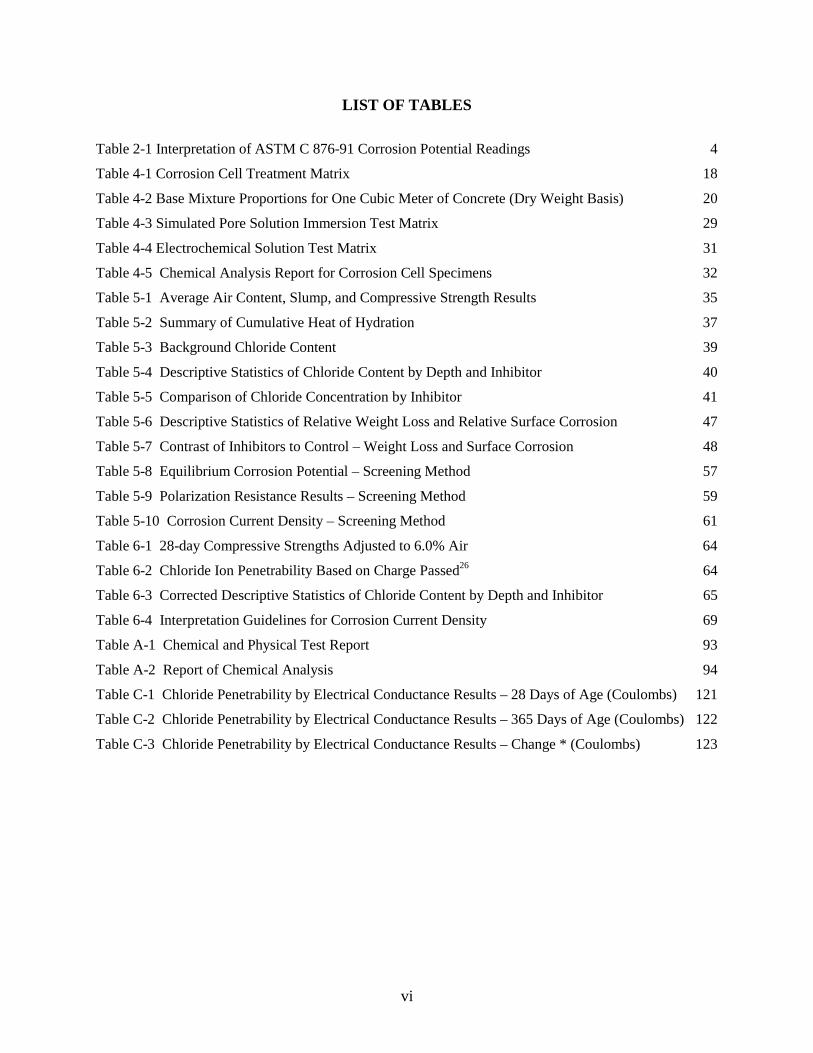
LIST OF TABLES Table 2-1 Interpretation of ASTM C 876-91 Corrosion Potential Readings 4 Table 4-1 Corrosion Cell Treatment Matrix 18 Table 4-2 Base Mixture Proportions for One Cubic Meter of Concrete (Dry Weight Basis) 20 Table 4-3 Simulated Pore Solution Immersion Test Matrix 29 Table 4-4 Electrochemical Solution Test Matrix 31 Table 4-5 Chemical Analysis Report for Corrosion Cell Specimens 32 Table 5-1 Average Air Content, Slump, and Compressive Strength Results 35 Table 5-2 Summary of Cumulative Heat of Hydration 37 Table 5-3 Background Chloride Content 39 Table 5-4 Descriptive Statistics of Chloride Content by Depth and Inhibitor 40 Table 5-5 Comparison of Chloride Concentration by Inhibitor 41 Table 5-6 Descriptive Statistics of Relative Weight Loss and Relative Surface Corrosion 47 Table 5-7 Contrast of Inhibitors to Control – Weight Loss and Surface Corrosion 48 Table 5-8 Equilibrium Corrosion Potential – Screening Method 57 Table 5-9 Polarization Resistance Results – Screening Method 59 Table 5-10 Corrosion Current Density – Screening Method 61 Table 6-1 28-day Compressive Strengths Adjusted to 6.0% Air 64 Table 6-2 Chloride Ion Penetrability Based on Charge Passed26 64 Table 6-3 Corrected Descriptive Statistics of Chloride Content by Depth and Inhibitor 65 Table 6-4 Interpretation Guidelines for Corrosion Current Density 69 Table A-1 Chemical and Physical Test Report 93 Table A-2 Report of Chemical Analysis 94 Table C-1 Chloride Penetrability by Electrical Conductance Results – 28 Days of Age (Coulombs) 121 Table C-2 Chloride Penetrability by Electrical Conductance Results – 365 Days of Age (Coulombs) 122 Table C-3 Chloride Penetrability by Electrical Conductance Results – Change * (Coulombs) 123

vii

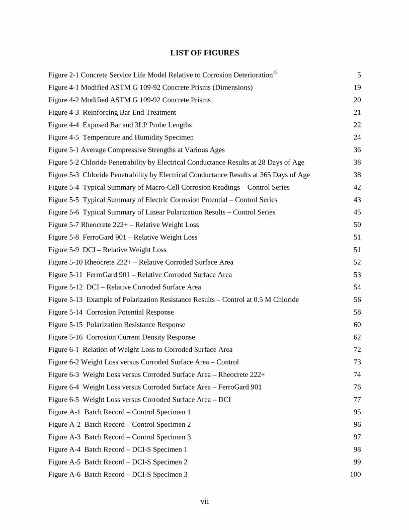
LIST OF FIGURES Figure 2-1 Concrete Service Life Model Relative to Corrosion Deterioration15 5 Figure 4-1 Modified ASTM G 109-92 Concrete Prisms (Dimensions) 19 Figure 4-2 Modified ASTM G 109-92 Concrete Prisms 20 Figure 4-3 Reinforcing Bar End Treatment 21 Figure 4-4 Exposed Bar and 3LP Probe Lengths 22 Figure 4-5 Temperature and Humidity Specimen 24 Figure 5-1 Average Compressive Strengths at Various Ages 36 Figure 5-2 Chloride Penetrability by Electrical Conductance Results at 28 Days of Age 38 Figure 5-3 Chloride Penetrability by Electrical Conductance Results at 365 Days of Age 38 Figure 5-4 Typical Summary of Macro-Cell Corrosion Readings – Control Series 42 Figure 5-5 Typical Summary of Electric Corrosion Potential – Control Series 43 Figure 5-6 Typical Summary of Linear Polarization Results – Control Series 45 Figure 5-7 Rheocrete 222+ – Relative Weight Loss 50 Figure 5-8 FerroGard 901 – Relative Weight Loss 51 Figure 5-9 DCI – Relative Weight Loss 51 Figure 5-10 Rheocrete 222+ – Relative Corroded Surface Area 52 Figure 5-11 FerroGard 901 – Relative Corroded Surface Area 53 Figure 5-12 DCI – Relative Corroded Surface Area 54 Figure 5-13 Example of Polarization Resistance Results – Control at 0.5 M Chloride 56 Figure 5-14 Corrosion Potential Response 58 Figure 5-15 Polarization Resistance Response 60 Figure 5-16 Corrosion Current Density Response 62 Figure 6-1 Relation of Weight Loss to Corroded Surface Area 72 Figure 6-2 Weight Loss versus Corroded Surface Area – Control 73 Figure 6-3 Weight Loss versus Corroded Surface Area – Rheocrete 222+ 74 Figure 6-4 Weight Loss versus Corroded Surface Area – FerroGard 901 76 Figure 6-5 Weight Loss versus Corroded Surface Area – DCI 77 Figure A-1 Batch Record – Control Specimen 1 95 Figure A-2 Batch Record – Control Specimen 2 96 Figure A-3 Batch Record – Control Specimen 3 97 Figure A-4 Batch Record – DCI-S Specimen 1 98 Figure A-5 Batch Record – DCI-S Specimen 2 99 Figure A-6 Batch Record – DCI-S Specimen 3 100

viii

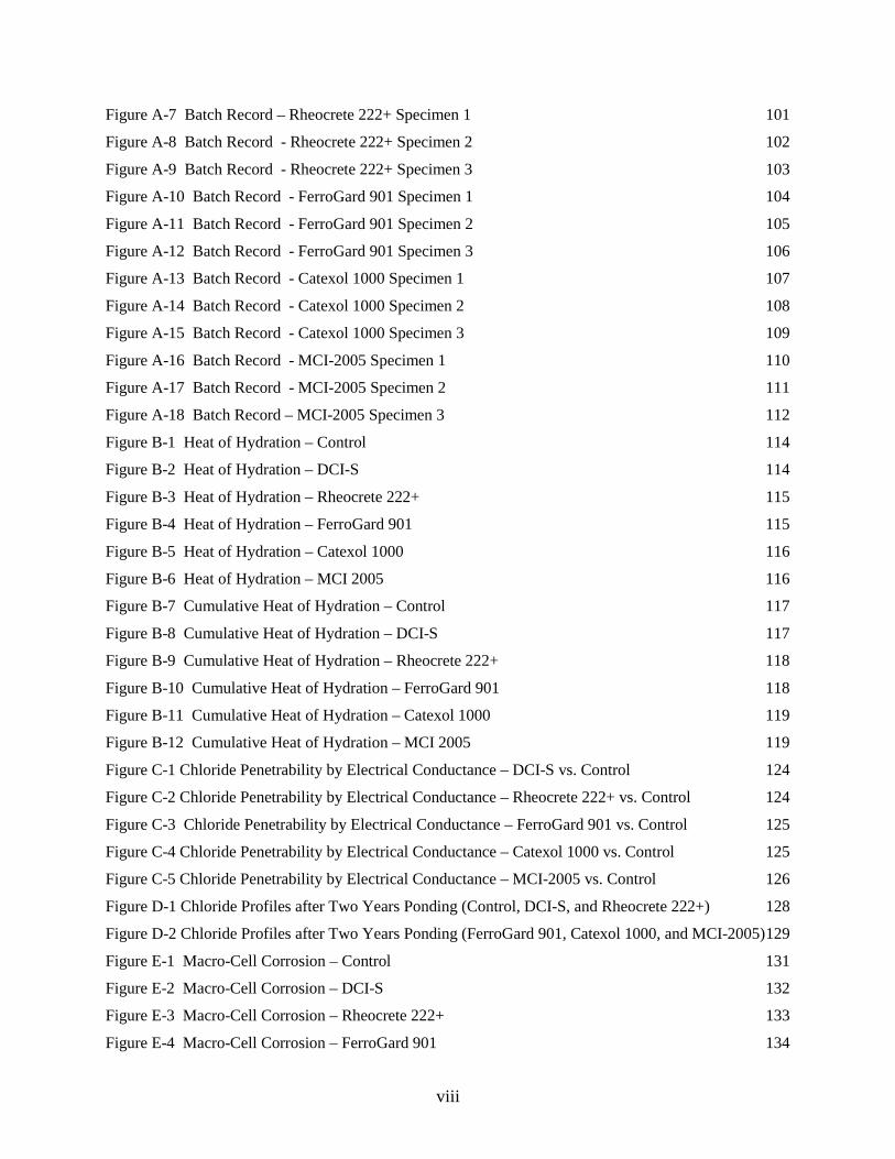
Figure A-7 Batch Record – Rheocrete 222+ Specimen 1 101 Figure A-8 Batch Record - Rheocrete 222+ Specimen 2 102 Figure A-9 Batch Record - Rheocrete 222+ Specimen 3 103 Figure A-10 Batch Record - FerroGard 901 Specimen 1 104 Figure A-11 Batch Record - FerroGard 901 Specimen 2 105 Figure A-12 Batch Record - FerroGard 901 Specimen 3 106 Figure A-13 Batch Record - Catexol 1000 Specimen 1 107 Figure A-14 Batch Record - Catexol 1000 Specimen 2 108 Figure A-15 Batch Record - Catexol 1000 Specimen 3 109 Figure A-16 Batch Record - MCI-2005 Specimen 1 110 Figure A-17 Batch Record - MCI-2005 Specimen 2 111 Figure A-18 Batch Record – MCI-2005 Specimen 3 112 Figure B-1 Heat of Hydration – Control 114 Figure B-2 Heat of Hydration – DCI-S 114 Figure B-3 Heat of Hydration – Rheocrete 222+ 115 Figure B-4 Heat of Hydration – FerroGard 901 115 Figure B-5 Heat of Hydration – Catexol 1000 116 Figure B-6 Heat of Hydration – MCI 2005 116 Figure B-7 Cumulative Heat of Hydration – Control 117 Figure B-8 Cumulative Heat of Hydration – DCI-S 117 Figure B-9 Cumulative Heat of Hydration – Rheocrete 222+ 118 Figure B-10 Cumulative Heat of Hydration – FerroGard 901 118 Figure B-11 Cumulative Heat of Hydration – Catexol 1000 119 Figure B-12 Cumulative Heat of Hydration – MCI 2005 119 Figure C-1 Chloride Penetrability by Electrical Conductance – DCI-S vs. Control 124 Figure C-2 Chloride Penetrability by Electrical Conductance – Rheocrete 222+ vs. Control 124 Figure C-3 Chloride Penetrability by Electrical Conductance – FerroGard 901 vs. Control 125 Figure C-4 Chloride Penetrability by Electrical Conductance – Catexol 1000 vs. Control 125 Figure C-5 Chloride Penetrability by Electrical Conductance – MCI-2005 vs. Control 126 Figure D-1 Chloride Profiles after Two Years Ponding (Control, DCI-S, and Rheocrete 222+) 128 Figure D-2 Chloride Profiles after Two Years Ponding (FerroGard 901, Catexol 1000, and MCI-2005) 129 Figure E-1 Macro-Cell Corrosion – Control 131 Figure E-2 Macro-Cell Corrosion – DCI-S 132 Figure E-3 Macro-Cell Corrosion – Rheocrete 222+ 133 Figure E-4 Macro-Cell Corrosion – FerroGard 901 134

ix

Figure E-5 Macro-Cell Corrosion – Catexol 1000 135 Figure E-6 Macro-Cell Corrosion – MCI 2005 136 Figure E-7 Electric Potential – Control 137 Figure E-8 Electric Potential – DCI-S 138 Figure E-9 Electric Potential – Rheocrete 222+ 139 Figure E-10 Electric Potential – FerroGard 901 140 Figure E-11 Electric Potential – Catexol 1000 141 Figure E-12 Electric Potential – MCI 2005 142 Figure E-13 Linear Polarization – Control 143 Figure E-14 Linear Polarization – DCI-S 144 Figure E-15 Linear Polarization – Rheocrete 222+ 145 Figure E-16 Linear Polarization – FerroGard 901 146 Figure E-17 Linear Polarization – Catexol 1000 147 Figure E-18 Linear Polarization – MCI 2005 148 Figure E-19 Temperature – Control and DCI-S 149 Figure E-20 Temperature – Rheocrete 222+ and FerroGard 901 150 Figure E-21 Temperature – Catexol 1000 and MCI 2005 151 Figure E-22 Relative Humidity – Control and DCI-S 152 Figure E-23 Relative Humidity – Rheocrete 222+ and FerroGard 901 153 Figure E-24 Relative Humidity Catexol 1000 and MCI 2005 154 Figure F-1 Polarization Resistance Screening Method – Control (Base) 158 Figure F-2 Polarization Resistance Screening Method – DCI (Base) 159 Figure F-3 Polarization Resistance Screening Method – DCI (Extended) 160 Figure F-4 Polarization Resistance Screening Method – FerroGard 901 (Extended) 161 Figure F-5 Polarization Resistance Screening Method – Rheocrete 222+ (Extended) 162

1

1 INTRODUCTION

On February 29, 1944, testimony began before the House Roads Committee on the legislation that would approve the National System of Interstate Highways. Commissioner Thomas MacDonald testified that, unlike wartime legislation, the proposal "is not temporary, but will mark the progress of road construction for the next quarter of a century." On June 25, 1952, President Harry Truman signed the Federal-Aid Highway Act, which authorized the first funding, $25 million, specifically for the Interstate System.1 Thus, America undertook the largest single public works project in history, the federal highway system. Construction of the new Interstate Highway system continued through the 1960's, amidst great fanfare and no small amount of controversy. Along with over 40,000 miles of pavement came the construction of an enormous number of bridges.

The need for cost effective systems for protection against corrosion has become increasingly clear since the first observations of severe corrosion damage to interstate bridges in the 1960’s. In response to public concern following the collapse of the Silver Bridge on December 15, 1967, the USDOT announced a comprehensive program to analyze the safety of over 703,000 highway and railroad bridges.1 Presently, corrosion of reinforcing steel in concrete exposed to chloride-laden environments is a well-known and documented phenomenon. The United States bridge system continues to experience severe deterioration and increasing maintenance demand as a result of corrosion related damage. The end result is premature end of service life or replacement, at high cost to taxpayers.

Since the mid 1960’s, several methods have been investigated to extend the time to corrosion damage in structures. Efforts have included tighter quality control on materials and construction practices, design modifications, such as increased concrete cover over reinforcing steel, and the use of specialized systems for corrosion prevention. Such systems include epoxy and galvanized coatings of reinforcing steel, active and passive cathodic protection systems, and use of corrosion inhibiting admixtures in concrete. Cathodic protection systems have been proven to be effective, but, require constant monitoring to ensure effectiveness and, depending upon the application, may be maintenance intensive and expensive to install.2,3 Epoxy coating of steel became the corrosion prevention method of choice in the late 1970's.4,5 However, studies in recent years have begun to question the long-term efficacy of epoxy coating systems toward corrosion durability.6,7 As time has passed, the use of corrosion inhibitors has become more common in preventing or delaying corrosion related damage in reinforced concrete structures. Still, many corrosion inhibiting admixtures on the market today have not undergone adequate testing and lack long-term track records necessary to justify their use in structures expected to be in service for 75 years or more.8 More research is necessary to determine which products are effective, and better tools are needed for evaluating potential products in a time frame far shorter than the service life over which they are expected to perform. This study addresses performance of corrosion inhibiting admixtures and methods for evaluating them.

2

2 BACKGROUND

Concrete Reinforcement Corrosion

The issue of reinforcement corrosion in reinforced concrete structures gained national attention shortly after the advent of the interstate highway system. Before the major highway development period of the 1950's and 1960's was complete, severe deterioration of structures less than 20 years of age was noted. In the ensuing years, the primary cause of this premature deterioration was subsequently identified as corrosion of the embedded reinforcing steel as the result of chloride contamination and carbonation of poorer quality concrete.

By the 1970's, much effort was being focused on identifying methods for protecting the reinforcing steel from these phenomena, as well as to improve the quality of concrete used in highway construction and limit the amount of aggressive agents present in the construction materials. Popular corrosion prevention techniques since that time have included epoxy coating of reinforcing steel, galvanized coatings of steel, and the use of corrosion inhibiting admixtures in concrete.

Concrete admixtures, in general, have been in use for decades to address material properties, such as air content, water reduction, increased workability, acceleration and retarding of hydration, and ultimate strength. Specific chemical admixtures have been developed over the last 15 to 20 years to address the phenomenon of reinforcement corrosion. Many have not been effectively evaluated through independent assessments in laboratory or field applications.

Corrosion Mechanism in Concrete

In order to assess the relative performance of corrosion inhibitors in varying laboratory applications, it is necessary to have a basic understanding of the underlying reactions involved.

Electrochemical Process

In general, the most prevalent deterioration mechanisms of reinforcement corrosion involve chloride ions, as found in salts, or the reduction of pH in concrete as a result of carbonation of the cement binder. Chloride ions may be contained in the original constituents of concrete, from mixing water, aggregate or admixtures, or they may be absorbed from the environment into the concrete matrix during the life of the structure. In current practice, efforts are generally made to minimize the amount of chloride in concrete constituents, so the majority of chloride that results in deterioration is derived from the environment. Environmental sources of chloride include seawater, ground water, or salts used in deicing operations during winter months. Over time, chloride ions or compounds penetrate through the cover concrete to the depth of the reinforcement through a process called diffusion.2

A simple model of the chemical reactions associated with corrosion deterioration of steel within concrete follows. Oxidization of iron (Fe++) molecules naturally occurs immediately after the bar is manufactured and exposed to the atmosphere, and will continue so long as sufficient oxygen and moisture are available to react with the steel. Upon exposure to the high pH environment of concrete, a passive layer of oxidation product forms on the encapsulated steel surface. This passivation process is actually a form of corrosion. However, in the moist, high

3

pH environment of concrete, the reaction occurs at an ever-decreasing rate.9 In the absence of aggressive ions, oxidation nearly ceases after a sufficient passive layer has formed. The passive layer normally protects the reinforcement from spontaneous corrosion in a moist, oxygen-rich environment such as concrete. However, chloride ions (Cl-) that diffuse to the steel surface can disrupt the passive layer and induce corrosion. Generally, metal atoms pass into solution as positively charged ions at the anodic site and liberated electrons flow through the metal to cathodic sites where dissolved oxygen is available to consume them.

For example, chloride ions react with iron compounds in the passive layer to create an iron-chloride complex (FeCl2), which subsequently reacts with hydroxide (OH-) from the surrounding concrete to form hydrated iron oxide compounds. This is commonly known as the anodic reaction. Simultaneously, at an alternate location on the steel surface, oxygen (O2) reacts with water (H2O) and electrons released by the anodic reaction to form hydroxide. This is referred to as the cathodic reaction. Together, the anodic reaction and the cathodic reaction form a corrosion cell.10

Many corrosion cells may exist along the same steel member and within a concrete member simultaneously. Localized corrosion, or micro-cell corrosion, involves anode and cathode reactions occurring adjacent to one another on the same surface. Macro-cell corrosion cells involve anode and cathode reactions occurring at distant locations on the same element or on different bars, or metal elements, that are electrically continuous.

Collectively, the anodic and cathodic reactions must be balanced. Therefore, in order for the reactions to occur at the same rate, a balance of the following elements is required:

• Iron (Fe++) - provided by the reinforcing steel

• Chloride (Cl-) - from the environment or concrete constituents

• Oxygen (O2) - from the environment

• Water (H2O) - from concrete and environment

A crucial characteristic of the corrosion mechanism is that the hydrated iron oxide compounds occupy greater volume than the original reactants, the exact proportion depending upon the composition of the compounds and conditions of the confining environment. As the volume of accumulated reaction products increases, pressure is generated within the concrete, which may ultimately exceed the tensile capacity of the concrete and result in cracking, delamination and spalling.2,11

Electrical Potential

Once chloride has reached the reinforcing steel in concentrations above the threshold limit (typically 0.6 to 1.2 kilograms of chloride ion per cubic meter of concrete for uninhibited systems)12,9, the deterioration of the passive layer initiates, and the corrosion process begins. Research has shown that the arrival of sufficient chloride to initiate sustained corrosion is marked shortly thereafter by a sharp increase in the magnitude of electrical potential of the reinforcing steel, as measured against a standard reference probe, such as a copper-copper sulfate electrode (CSE) or standard calomel electrode (SCE).13

4

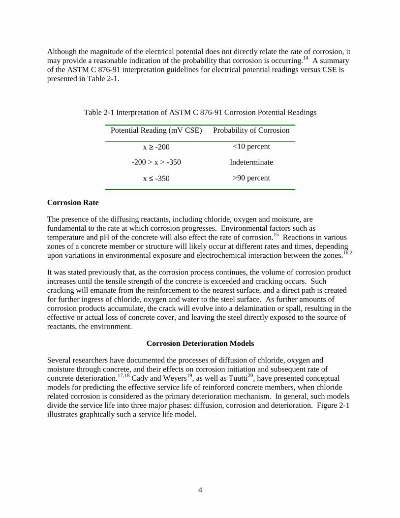
Although the magnitude of the electrical potential does not directly relate the rate of corrosion, it may provide a reasonable indication of the probability that corrosion is occurring.14 A summary of the ASTM C 876-91 interpretation guidelines for electrical potential readings versus CSE is presented in Table 2-1.

Table 2-1 Interpretation of ASTM C 876-91 Corrosion Potential Readings

Potential Reading (mV CSE) Probability of Corrosion

x ≥ -200 <10 percent

-200 > x > -350 Indeterminate

x ≤ -350 >90 percent

Corrosion Rate

The presence of the diffusing reactants, including chloride, oxygen and moisture, are fundamental to the rate at which corrosion progresses. Environmental factors such as temperature and pH of the concrete will also effect the rate of corrosion.15 Reactions in various zones of a concrete member or structure will likely occur at different rates and times, depending upon variations in environmental exposure and electrochemical interaction between the zones.16,2

It was stated previously that, as the corrosion process continues, the volume of corrosion product increases until the tensile strength of the concrete is exceeded and cracking occurs. Such cracking will emanate from the reinforcement to the nearest surface, and a direct path is created for further ingress of chloride, oxygen and water to the steel surface. As further amounts of corrosion products accumulate, the crack will evolve into a delamination or spall, resulting in the effective or actual loss of concrete cover, and leaving the steel directly exposed to the source of reactants, the environment.

Corrosion Deterioration Models

Several researchers have documented the processes of diffusion of chloride, oxygen and moisture through concrete, and their effects on corrosion initiation and subsequent rate of concrete deterioration.17,18 Cady and Weyers19, as well as Tuutti20, have presented conceptual models for predicting the effective service life of reinforced concrete members, when chloride related corrosion is considered as the primary deterioration mechanism. In general, such models divide the service life into three major phases: diffusion, corrosion and deterioration. Figure 2-1 illustrates graphically such a service life model.

5

Figure 2-1 Concrete Service Life Model Relative to Corrosion Deterioration15

Note that some initial deterioration is predicted, related to damage that often occurs during construction during handling and placement of constituents. This is to say that no structure begins service in perfect condition. The diffusion phase, or time-to-corrosion, can be thought of as initiating either when the member is first placed into service or first exposed to a source of chloride contaminant. This phase represents the period of time during which chloride diffuses through the cover concrete and accumulates at the surface of the reinforcing steel. Although in most cases diffusion of chloride continues and concentrations continue to increase at the steel surface, the diffusion phase is generally considered to end at the point at which the amount of chloride at the steel surface is sufficient to initiate corrosion. Hence, the corrosion phase begins.

The corrosion phase, or time-to-cracking, involves the steady build-up of corrosion product within the existing void space around the reinforcing steel in the concrete. Corrosion continues until sufficient corrosion product has been produced to cause cracking of the cover concrete. During the final deterioration phase, or time to end of functional service life, the concrete deteriorates to a point deemed unacceptable for use. This amount of corrosion related damage is somewhat subjective, and will vary not only according to the deciding authority, but also relative to the nature and purpose of the concrete member in question.21,22

Corrosion deterrence efforts usually include both deterrence of aggressive ion intrusion and inhibition of corrosion reaction(s) once contaminants reach the steel reinforcement. The International Organization for Standardization (ISO) defines a corrosion inhibitor as a “Chemical substance which decreases the corrosion rate when present in the corrosion system at a suitable concentration, without significantly changing the concentration of any other corrosive agent.”

6

The following summary is paraphrased from Hansson, who stated that admixtures used to deter corrosion function by: 23

1. Increasing the resistance of the passive film on the steel to breakdown by chloride (increasing the chloride threshold value and reducing corrosion rate, thereby increasing the time to corrosion and cracking);

2. Creating a barrier film on the steel (increasing the chloride threshold value and reducing corrosion rate, thereby increasing the time to corrosion and cracking);

3. Scavenging the oxygen dissolved in the pore solution (decreasing the corrosion rate, thereby increasing the time-to-cracking);

4. Blocking ingress of chlorides (decreasing the rate of diffusion, thereby increasing the time-to-corrosion);

5. Increasing the degree of chloride binding in the concrete (decreasing chloride concentration within the pore solution, thereby increasing the time-to-corrosion);

6. Blocking the ingress of oxygen (decreasing the corrosion rate, thereby increasing the time-to-cracking).

Strictly speaking, only items 1, 2 and 3 above can be functions of “inhibitors” according to the ISO definition. The latter three functions are not considered inhibition, but represent physical processes for limiting the availability of reactants to delay the onset of corrosion. The diffusion and corrosion phases are discussed in detail in the following sections.

Chloride Diffusion Model

Previous research has focused on determining the rate at which chloride progresses through concrete to reach embedded reinforcing steel.20,11 Methods have been developed to predict the time of arrival of the contaminant and the subsequent time of active corrosion necessary to induce cracking.24

Permeability

The most important material characteristic of concrete in resisting chloride ingress is the material permeability. Much research has been conducted to determine the internal pore structure of portland cement concrete and its effect on chloride permeability.17 It is commonly known that as concrete ages and continues to hydrate, the permeability of the material changes. Continuing hydration reduces permeability, but carbonation of concrete exposed to carbon dioxide in the atmosphere will increase permeability. The terminology "permeability" and "porosity" are often mistakenly used interchangeably. Although in many materials the two characteristics are often proportional to one another, it should be noted that it is possible to have a material that is highly porous, yet relatively impermeable. This is often true of concrete and concrete aggregates.

Currently, convenient methods are not available to directly measure the permeability of concrete to water and chloride ions. The permeability of concrete is often monitored indirectly by measuring the conduction of electrical current through saturated concrete specimens under controlled conditions, as specified in ASTM C 1202-94, Standard Test Method for Electrical Indication of Concrete's Ability to Resist Chloride Ion Penetration. This method has gained

7

standard acceptance, but critics emphasize that material composition and the presence of various ions, including certain admixture components, within the pore structure may significantly influence results.25,26 In particular, ASTM C 1202-94, Section 5 – Interferences states that misleading results are possible when calcium nitrite (the active ingredient in DCI) has been admixed into concrete. Such concrete has yielded higher coulomb values under the test, implying lower resistance to chloride ion penetration. Results of longer chloride ponding tests have shown concrete with calcium nitrite is at least as resistant to chloride penetration as control mixtures.

Fick’s Laws

The most commonly recognized principles for the transport of chloride ions, and other reactants, from the surface of concrete to the embedded steel are the Laws of Diffusion first discovered by Adolf Fick in 1855. Modeling of the process is based on kinetic theory and the random motion of molecules.27 The most important notion of Fick’s Laws relative to chloride diffusion is that movement of the diffusing substance occurs from a region of high concentration to one of lower concentration.

Under certain conditions, capillary action can significantly influence the ingress of contaminants or reactants into a porous structure.17,28,22 However, in the case of moderate to good quality concrete, the influence of capillarity below the surface layer of concrete is only significant in those cases where the concrete is relatively dry. Parrott reported that the general trend of relative humidity for horizontal concrete specimens exposed to an outdoor environment, similar to that of a bridge deck, fluctuates in the range of 80 to 100 percent, with no major effect of depth.29 In fact, at relative humidities below 100%, but well above 90%, most of the large capillaries (>50nm) within portland cement concrete begin to lose water, leaving discontinuity of solution between the smaller capillaries and interstitial pore spaces.30 Therefore, capillarity does not play a significant role in most climates where significant deicing salt or seawater related corrosion exists.

Temperature, atmospheric pressure and relative humidity are constantly in flux in field environments. As a result, other mechanisms of transport, such as convection or pressure gradients, do not contribute a continuous driving force for the infusion of chloride into concrete and have a less direct influence on chloride diffusion in concrete field specimens. However, in bridge decks exposed to a salt-laden environment, the chloride concentration becomes relatively stable below approximately 13 millimeters depth into the cover concrete, and becomes the driving concentration that causes diffusion.10,19 The presence of significant free pore water solution within smaller concrete capillaries provides sufficient medium for transport of ionic species under diffusive pressures formed by the concentration gradient.

8

Fick's First Law of Diffusion states that the rate of flow of molecules is proportional to the change in concentration per unit distance (called the concentration gradient) and can be expressed mathematically in its simplest form as:27

Equation 2-1

where; J = the rate of flow (kg/mm2⋅year) Dc = the diffusion constant (mm2/year) dC = the incremental change in concentration (kg/mm3) dx = the incremental change in distance (mm)

Note that Equation 2-1 does not specifically address time as a variable, yet it is obvious that time is the most important focus in assessing the life expectancy of reinforced concrete exposed to corrosive environments. Fick's Second Law of Diffusion addresses the time dimension of the diffusion problem and is expressed most simply as:

Equation 2-2

where; C = concentration at a given point along a path (kg/mm3) t = time (years) x = distance (mm)

Diffusion Constant

Concrete researchers have refined the diffusion model, taking into consideration the boundary conditions in a concrete environment. Weyers applied a mathematical solution of Equation (2), based on the boundary condition of chloride concentration near the surface, C0, as a function of the square root of time, to model the ingress of chloride into concrete surfaces, such as bridge deck.31 The time dependent characteristic of near-surface chloride concentration has been found to be appropriate for laboratory specimens which have not undergone extensive environmental exposure prior to testing.

Equation 2-3

where; C(x,t) = chloride concentration at depth x after exposure time t k = coefficient dependent upon concrete material and surface concentration erf = mathematical error function32

Using Equation 2-3, diffusion constants can be derived from a least-squares regression fit of chloride profiles obtained in laboratory testing.

2

2

xCD

tC

c ∂∂=

∂∂

−−=

−

tDxerf

tDxetkC

cc

tDx

txc

21

24

),(

2

π

dxdCDJ c−=

9

The near surface chloride content for field specimens which have been in service for several years may be modeled by a constant value of C0. Therefore, the system may be modeled by the simplified equation:

Equation 2-4

where; C0 = constant chloride concentration near the surface

Corrosion Threshold

For uninhibited reinforced concrete systems, the threshold concentration necessary to initiate sustained corrosion lies approximately between 0.6 and 1.2 kilograms of chloride per cubic meter of concrete.12,9 Therefore, the presence of chloride concentrations at the reinforcement depth in excess of approximately 1.2 kilograms per cubic meter of concrete will likely reduce the life expectancy of the system and may warrant premature rehabilitation or replacement of the contaminated concrete.

Time-to-Cracking

Over the past decade, much effort has been placed on characterizing the rate of corrosion of reinforcing steel in concrete and quantifying the subsequent time to cracking of the cover concrete. Empirical and theoretical models have been developed to predict the time to corrosion related cracking of concrete cover and subsequent end of functional service life.22,31

Corrosion Rate

Once diffusion has occurred and corrosion has initiated, the most significant factor affecting remaining service life of a structure is the corrosion rate. It is well known that corrosion rate varies widely depending on environmental conditions including availability of oxygen within the concrete, moisture content of a concrete, temperature, as well as physical characteristics of the corrosion process. For example, as corrosion product accumulates on the reinforcing steel surface, reactants diffuse more slowly through the corrosion products to the virgin steel. If oxygen is slower to diffuse to the steel surface, the rate of the cathodic reaction is reduced, and the overall reaction is likewise reduced.2 Also, as corrosion progresses and the cumulative area of anodic reaction sites increases on the bar surface, less area is available for the balancing cathodic reaction, resulting in a reduction of corrosion rate.

Corrosion Products

A key factor in developing the regression model for time to cracking involves determination of the critical mass of corrosion products necessary to initiate cracking. It is commonly known that corrosion products of reinforcing steel exceed the volume of initial reactants. The exact ratio of product volume to reacted volume varies considerably, as does the composition of the rust products, depending on environmental factors, steel composition, oxygen and moisture availability, and rate of corrosion.15 One step in the modeling process must consider the amount of corrosion product necessary to induce stress in excess of the tensile capacity of the cover

−=

tDxerfCC

ctx 2

10),(

10

concrete. In establishing this critical mass of corrosion product, it is necessary to consider concrete material properties which effect the amount of total strain which the concrete will undergo prior to cracking, as well as the presence of void volume present around the reinforcing steel within the cement paste matrix.

Bazant model

Bazant presented a systematic mathematical model for predicting time to cracking as a function of diffusion of oxygen, chloride ions, pore water, and ferrous hydroxide.11 The model also considered critical chloride concentration, electric potential and current flow through electrolyte, and mass/volume relations that affect the rate of rust production at the reinforcing steel surface. The details of Bazant's model are too lengthy to discuss in detail in this work, but the reader should be aware of its existence. In all, Bazant's model involved a series of 13 equations to describe the complex diffusionary processes, chemical reactions, and electrochemical interactions involved in concrete reinforcing steel corrosion.

Bazant's model is based on theoretical physical models, and it has never been fully validated experimentally. In a recent study, Newhouse and Weyers noted that the model significantly underestimated time to corrosion cracking under laboratory and field conditions.33

Liu-Weyers model

Liu and Weyers developed an empirical model for the time-to-cracking based on Faraday's Law and critical mass of corrosion products.24 The model uses corrosion current density measurements available through modern test equipment to establish an effective rate of corrosion, typically expressed in units of surface penetration distance versus time. The model was generated by statistical analysis of data gathered from indoor and outdoor laboratory specimens over a period of five years. A regression equation was developed which demonstrated that corrosion rate could be effectively predicted as a function of chloride content, temperature at reinforcement depth, ohmic resistance of concrete, and time of exposure. By applying documented chloride content, temperature, concrete ohmic resistance, and periodic measurements of instantaneous corrosion rate, in concert with Faraday's law and characteristic data about the structural element in question, it was shown that this predictive equation could be used to project the approximate time-to-cracking for outdoor exposure specimens.

Corrosion Deterrence and Mitigation

Methods of Corrosion Deterrence

Since the 1960's, many methods toward corrosion prevention have been investigated, with mixed success. Following are a few of the more popular or more successful methods that have been employed.

Steel surface treatments

Several different types of surface treatments have been investigated in recent decades. In the 1970's, the coating of reinforcing steel with epoxy was established as the primary means for corrosion deterrence.5 Recent studies of bridges and structures that incorporated epoxy coated

11

steels built during that time suggest that epoxy coating may not provide the 75-year service life that was predicted.7,34

Another method of steel surface treatment is galvanizing, or zinc coating. However, this treatment has shown mixed results in concrete and may be inadequate for desired service life performance in many environments.2

Alternative materials

Alternative materials for reinforcing steel have been considered and tested. However many of these materials are generally disqualified based on cost or safety requirements. Stainless steels provide a corrosion resistant alternative to conventional steel, but at considerable expense.2 Other structural materials, including fiber-polymer composites, are generally considered undesirable for use as concrete reinforcement since they are brittle and do not possess the yield characteristics of steel. Overstressing or fatigue of brittle materials may present a potential for catastrophic failure, without the visible warning afforded by ductile steels.

Concrete surface treatments

The use of surface coatings for concrete members, including polymer membranes, penetrating sealers, and modified cementitious or acrylic coatings, has often been used to supplement existing corrosion prevention strategies. Indeed, quality surface treatments may prevent the ingress of aggressive species, including chlorides, as well as the diffusion of reactants necessary to sustain corrosion. However, such coatings are often maintenance intensive. Surface coatings are inadequate to prevent corrosion once the aggressive species have penetrated the concrete, since there is generally sufficient moisture within concrete to sustain corrosion for an extended period of time. A properly selected and applied coating may reduce the rate of ingress of oxygen, thereby slowing the rate of reaction, but by no means eliminates the occurrence of corrosion.2,5

Concrete admixtures

Effects beneficial to chloride exclusion have been seen from addition of pozzolans in the creation of high-performance concrete. However, traditionally corrosion inhibiting admixtures have been defined as those chemical compounds which, when added to fresh concrete, will provide some level of protection via active chemical interaction with the potential corrosion reactants.

Corrosion Inhibitors

The focus of the current study is to assess the effectiveness of corrosion inhibiting admixtures. Generally, inhibiting admixtures are classified as anodic, cathodic, or mixed inhibitors. This convention reflects the relative location of inhibitor action within the electrochemical cell: at the anode, at the cathode, or both. Anodic inhibitors repress the reaction at the anode sites by their ability to accept electrons. Anodic inhibitor effectiveness is directly dependent upon their concentration relative to chloride.35,36

12

Cathodic inhibitors indirectly slow the rate of reaction, often by precipitation at the cathodic sites of an electrochemical cell, or by limiting the availability of oxygen necessary for the cathodic reaction to occur. Mixed inhibitors perform by both methods.

Inhibitors may also be distinguished as passivation inhibitors, organic inhibitors or precipitation inhibitors. Most inhibitors function by providing a protective layer at the steel surface. The intended purpose is to raise the threshold of chloride concentration necessary to breach the layer and initiate corrosion.37

Passivation inhibitors are chemical oxidizing substances, such as nitrite, which promote the formation of a stable surface oxide, preventing further oxidation of the metal substrate. Organic inhibitors form a protective film of adsorbed molecules on the metal surface, which provide a barrier to the dissolution of the metal.37

Mailvaganam offered the following summary concerning corrosion inhibitors for reinforced concrete:35

"Each group (of inhibitors) may include materials that function by one of the following mechanisms: (a) formation of barrier layers (b) oxidation by passivation of the surface and (c) influencing the environment and contact with the metal. To be an effective corrosion inhibitor the selected chemical or mixture of chemicals should meet the following requirements:

• The molecules should possess strong electron acceptor or donor properties or both.

• Solubility should be such that rapid saturation of the corroded surface occurs without being readily leached out of the material.

• Induce polarization of the respective electrodes at relatively low current values.

• Be compatible with the intended system so that adverse side effects are not produced.

• Be effective at the pH and temperature of the environment in which it is used."

In addition to specific inhibition at the anodic or cathodic sites on the reinforcing steel, some inhibiting admixtures are believed to reduce the rate of chloride diffusion through the concrete. This added benefit is believed to be the result of alterations in the permeability of the material through interaction between the admixture and the cement paste constituents.38

Corrosion Inhibitor Performance

Commercial corrosion inhibitors for concrete are said to function by one or both of two mechanisms: by increasing the threshold concentration of aggressive species necessary for corrosion to occur or by reducing the rate of corrosion once corrosion has begun.

Since the deleterious effects of chloride were identified, much has been done in design and construction practice to limit the amount of chloride present in original construction materials. Therefore, the primary source of chloride in structures today is the surrounding environment, such as seawater, and salts used in deicing operations, which is the direct result of the national "bare roads" maintenance policy in effect since the 1960's.39,40 Alternative deicing substances

13

have also been investigated, but generally they are too difficult to obtain and cost prohibitive for common use.41,42,43,44

Slowing the intrusion through the concrete of aggressive species, such as chloride, is another potential benefit of concrete admixtures. Admixtures that slow the ingress of chlorides into concrete generally do so by either of two methods. Some function by "clogging" the internal pore structure of the concrete, to deter movement of foreign substances by absorption or diffusion. Nmai defined these as “passive inhibitors” (not to be confused with passivation inhibitors), although this process cannot be correctly termed as inhibition.45 Reduction in pore size, bridging of pores with an interpenetrating film, and lining of pores with compounds imparting hydrophobic properties were cited as potential methods for limiting chloride ingress. Other admixtures function by "scavenging", in which aggressive species or oxygen in pore solution are chemically combined or adsorbed, rendering them inert in the concrete environment.23 Admixtures used specifically to deter chloride ingress or scavenge corrosion reactants have met with little to moderate success, and generally the effects are proportion dependent and recede over time. Some admixtures that meet the ISO definition of “corrosion inhibitor” may also impart one or more of these other benefits in concrete, although it is not their primary function.

Active corrosion inhibitors may increase the concentration of chloride necessary to induce corrosion. Many of these form a film or coating at the surface of the steel, and may react with incoming chloride ions, to prevent interaction between the aggressive chloride ions and the passivated layer of oxidized iron which naturally protect the steel in the high pH concrete environment.23,37,39

Performance Assessment Methods

Many studies have been performed under both laboratory and field conditions to assess the method of corrosion deterioration and to attempt to predict the time necessary for corrosion to occur and sufficient damage to accumulate to render the structurally or functionally deficient.

Simulated Conditions

Through continued laboratory studies of concrete reinforcement corrosion, several generally accepted types of test specimens have evolved, which attempt to simulate the reinforced concrete environment, and provide accelerated testing for chloride induce corrosion behavior and prevention.

One popular test specimen is the concrete lollipop, which involves a single reinforcing steel bar suspended in the center of a cast concrete cylinder. The steel often projects from one end of the cylinder, to provide electrical contact for electrochemical monitoring.9 One common flaw with this type of test specimen, as with many other specimen types, is the potential for crevice corrosion to occur at the interface where the steel projects from the concrete, and steel, concrete and the surrounding environment converge. Further, this type of specimen involves only a single steel bar, and may not accurately emulate the distribution of corrosion cells common in a mat of steel bars or a structural member with several layers of steel.

14

A more commonly accepted method for emulating reinforced concrete members is the use of small reinforced concrete slabs or prisms, which often contain multiple steel bars of various configurations. ASTM G 109-92 is an industry accepted standard for evaluating corrosion performance of reinforced concrete elements, and involves the arrangement of steel in two layers within a concrete prism.46

More recently, methods common to the corrosion scientist in other disciplines, such as pipeline corrosion, have been adapted for use in simulating corrosion performance in concrete environments. The suspension of small individual steel specimens in extracted or simulated concrete pore water solution permits the application of advanced electrochemical test techniques to more directly assess the corrosion behavior of exposed steel, without the electrical interference (impedance or resistance) caused by the concrete in conventional specimens.47

Field Conditions

In addition to laboratory characterizations of the corrosion process, considerable effort has been put into characterizing the condition of structures and determining real world influences on corrosion deterioration of reinforced concrete. Many studies have been conducted on a variety of structures, including bridges, parking structures, highways and conventional building structures.21,22,25 Attempts have been made to correlate condition and exposure time information of field structures with the laboratory corrosion research results. While significant progress has been made, there is still much to be done in the field for predicting effective service lives for structures.

Much attention has been given to the direct performance of inhibitors, coatings, and other methods of corrosion prevention and mitigation. Still more needs to be known about how these systems effect the over all life-cycle of structures, and what influences, positive or negative, such systems may have on future rehabilitation or replacement costs. The presence of coatings or other inhibiting systems may in fact complicate evaluation efforts, and may also have a significant impact on requirements for application of repairs and overlays.

Finally, it is important to practicing engineers and constructors that the focus of efforts include not only on the science of corrosion prevention, but also on the economy of any solutions put into practice. Indeed, many products exist on the market which purportedly address all the problems related to corrosion of reinforcement in concrete structures, but the practicing engineer has very little practical information upon which to base decisions.

Importance of Statistical Analysis

Significance Testing

In any quality research program, researchers should make every effort to provide statistically sound results. Perhaps the researchers should remember to ask themselves the following questions when considering the results of their research:

• Are the results observed statistically significant?

• Are the results of practical significance?

15

The first question speaks directly to subject of statistical significance, which involves the design of an experimental program with sufficient sample size, such that experimental error and the natural variance of the phenomenon being measured may be quantified. A sample size of one unit provides no information about the range over which measured phenomena may occur, or where a particular sample result is within such a range.

Proper scientific experiments generally incorporate analysis of variance of the measured data to quantify these unknowns. A further reason for statistical analysis in a proper scientific evaluation is to establish repeatability. The researchers must determine whether a given response can be reliably duplicated under the conditions outlined in the test program.

A well-designed experimental plan can allow researchers to differentiate between random experimental error, variations between groups or treatments, variations between individual specimens, and variations due to procedures between different trials of an experiment.

It would appear from those criteria, that the more samples tested, the better the results. This may be true relative to statistical analysis; however, limitations on resources often dictate a much smaller sample size than might be desired under a purely statistical approach. Therefore, a balance is to be found to optimize sample size versus available resources.

16

3 PURPOSE & SCOPE

This report conveys the results of a three-part laboratory study of corrosion inhibiting admixtures in concrete. The purposes of the study include:

• Determining the influence of a series of commercially available corrosion inhibiting admixtures on general concrete handling, performance and durability properties not related to corrosion.

• Determining the effectiveness of corrosion inhibiting admixtures for reduction or prevention of corrosion of reinforcing steel in concrete, relative to untreated systems, under laboratory conditions.

• Conducting a short-term pore solution immersion test for inhibitor performance and relating the results to those of the more conventional long-term corrosion monitoring techniques that employ admixtures in reinforced concrete prisms.

• Determining whether instantaneous electrochemical techniques can be applied in screening potential inhibitor admixtures.

The inhibitors incorporated in this study include a passivation inhibitor based on a calcium nitrite solution, organic inhibitors containing esters and amines or amino alcohol, and other commercial inhibitors, whose active ingredients are considered by the manufacturers as proprietary and remain undisclosed. Direct comparison of competitive products is neither attempted nor intended. Each product is evaluated solely in comparison to performance of untreated systems.

Statistical Approach

The first consideration in developing an experimental test plan is the establishment of a firm statistical basis for comparison of results. For each type and series of testing involved in this research, a variety of treatment levels were established. Effort was made to select a statistically sound number of repeat units for each treatment, without creating a test plan that was too cumbersome to complete.

Most test results presented herein are the result of statistical analyses of variance, and data for both the mean value(s) and 95 percent confidence intervals are presented, where appropriate. Unless otherwise noted, all comparisons within this study have been made at a significance level of α=0.05, or 95 percent confidence. With the exception of the short-term electrochemical solution tests, most phases of the experiment have approximately six test samples of a given treatment and exposure type. This number of samples was deemed adequate to provide an indication of statistical variance for the tests, without creating an overwhelming workload.

Experimental Model

For each type of testing, a treatment matrix and an appropriate number of specimens for each treatment were established.

17

Long-term experimental test

Long-term experimental tests involve concrete specimens, each comprising two experimental cells. Each treatment series involved three specimens, each produced from a separate batch of material, based upon the same mixture proportions. Statistical comparison was to be performed both between batches and between individual cells within a batch, to allow analysis of the relative experimental error(s) between different treatments, between batches of the same treatment, and between cells within the same batch. Hence, a total of six cells were created to represent each inhibiting admixture treatment. Inhibitor dosages were determined according to each manufacturer's product recommendations.

Short-term characterization tests

One set of short-term characterization tests involved treatment of individual bar specimens suspended in solutions containing various treatment levels of both chloride and inhibitors. As a full matrix was impractical, a modified matrix was employed, based on dosage guidelines provided by the respective manufacturers. For each treatment, six repeat units were processed, to quantify experimental error between units.

A second short-term characterization test involved the treatment of small steel test samples in an electrochemical cell. As this technique was experimental in nature, a matrix was developed to assess performance of select admixtures, each at a standard dosage level, and each subject to two exposure levels of chloride in solution. Two repeat units were processed for each treatment and exposure level. During testing, two additional exposure levels were added for one admixture, to more accurately assess the extent of corrosion inhibition under the experimental test.

18

4 METHODS & MATERIALS

The evaluation of corrosion inhibiting admixtures (CIA’s) in this project involved the comparison of results from several methods. As a benchmark and ground-base test for the performance of CIA’s, specimens of reinforced portland cement concrete were created, similar to those specified in ASTM G 109-92.46 Long-term evaluation of selected inhibitors in simulated concrete pore solution was performed via immersion and subsequent visual and weight loss analyses. Short-term evaluation of inhibitors in a simulated pore solution was performed according to a proposed ASTM test method for CIA’s, using electrochemical linear polarization resistance techniques.

Concrete Corrosion Cells

The concrete benchmark tests involved a matrix of specimens incorporating five commercial CIA’s and a set of control specimens. The specimen matrix is presented in Table 4-1. The concrete corrosion cells are modified versions of the ASTM G 109-92 standard test specimen.

Table 4-1 Corrosion Cell Treatment Matrix

Inhibitor Dosage (L/m3) Number of Specimens

Control 0 3 DCI-S (W.R. Grace) 15 3 Rheogard 222+ (Master Builders) 5 3 FerroGard 901 (Sika) 10 3 Catexol 1000 (Axim) 15 3 MCI 2005 (Cortec) 1 3

Specimens

The deviation from ASTM G 109-92 standard specimens involves the incorporation of two separate reinforcement triads into a single cast concrete prism. Each cast specimen represents a single batch of concrete, and, therefore, allows comparison of within batch variations of performance. As indicated in the matrix, the series for each CIA incorporates 3 specimens, each containing two electrically isolated reinforcement triads.

The concrete prisms are 356 millimeters wide by 318 millimeters deep by 152 millimeters high in overall dimension. The reinforcing steel triads are 356 millimeters long bare #5 (14 millimeters diameter) deformed steel reinforcing bars in a triangular pattern, one on the top and two on the bottom, which extend approximately nineteen millimeters out of the front and back faces of the concrete prisms. The clear cover over the top bars is 25 millimeters for all specimens. The bottom bars are centered at a depth of 70 millimeters below the center of the top bars and 70 millimeters apart, on either side of the top bar and have a clear cover of 25 millimeters. A schematic diagram of the specimens is presented in Figure 4-1.

19

Figure 4-1 Modified ASTM G 109-92 Concrete Prisms (Dimensions)

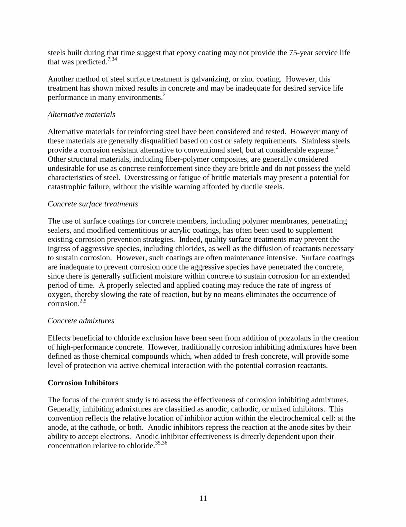
The two bottom reinforcing bars in each triad are connected with a jumper to make them electrically continuous, and the two bottom bars are connected to the top bar via a 100 ohm resistor between the front top and bottom right bar ends. The bars were protected to provide a known length of exposed steel surface within the concrete and to prevent crevice corrosion. See Figure 4-2.

The concrete mixtures were proportioned in accordance with the Virginia Department of Transportation’s standard specification A4 concrete for bridge decks. The water-to-cement ratio (w/c) for each mix was 0.45, and the mixtures contained 377.5 kilograms of cement per cubic meter of concrete. Air content and slump ranges were 3 to 5 percent and 75 to 100 millimeters, respectively. Generally, high-range water reducing admixtures (HRWR) and air entraining admixtures (AEA) were of the same brand as the subject CIA. Otherwise, appropriate admixtures from W.R. Grace were employed.

20

Figure 4-2 Modified ASTM G 109-92 Concrete Prisms

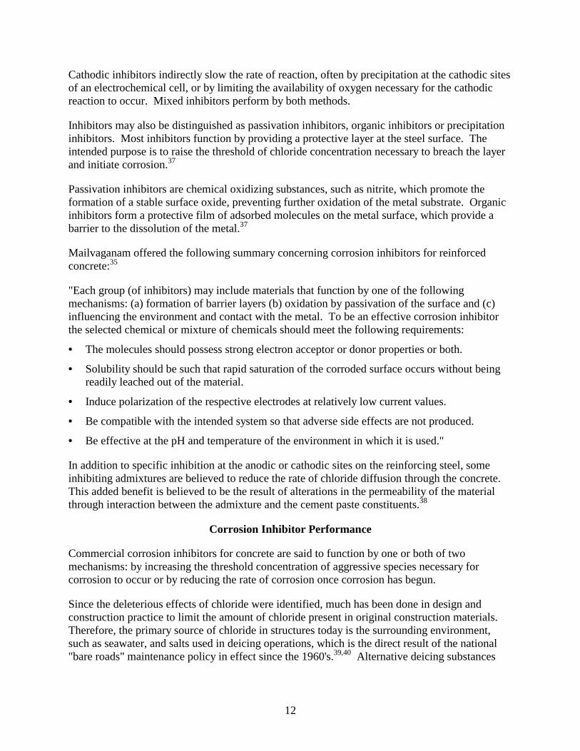
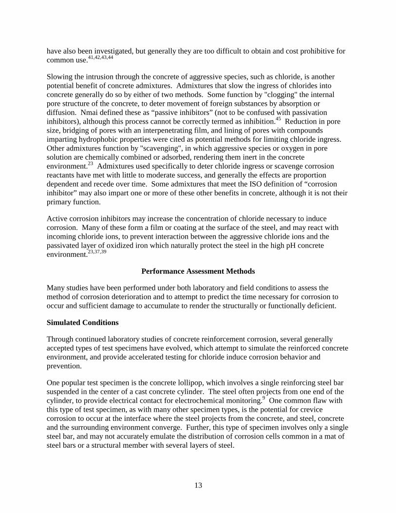
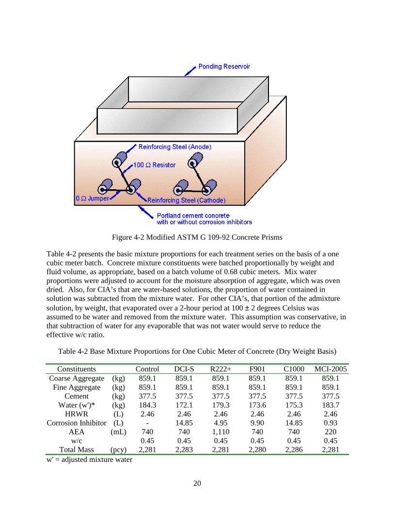
Table 4-2 presents the basic mixture proportions for each treatment series on the basis of a one cubic meter batch. Concrete mixture constituents were batched proportionally by weight and fluid volume, as appropriate, based on a batch volume of 0.68 cubic meters. Mix water proportions were adjusted to account for the moisture absorption of aggregate, which was oven dried. Also, for CIA’s that are water-based solutions, the proportion of water contained in solution was subtracted from the mixture water. For other CIA’s, that portion of the admixture solution, by weight, that evaporated over a 2-hour period at 100 ± 2 degrees Celsius was assumed to be water and removed from the mixture water. This assumption was conservative, in that subtraction of water for any evaporable that was not water would serve to reduce the effective w/c ratio.

Table 4-2 Base Mixture Proportions for One Cubic Meter of Concrete (Dry Weight Basis)

Constituents Control DCI-S R222+ F901 C1000 MCI-2005 Coarse Aggregate (kg) 859.1 859.1 859.1 859.1 859.1 859.1 Fine Aggregate (kg) 859.1 859.1 859.1 859.1 859.1 859.1

Cement (kg) 377.5 377.5 377.5 377.5 377.5 377.5 Water (w')* (kg) 184.3 172.1 179.3 173.6 175.3 183.7

HRWR (L) 2.46 2.46 2.46 2.46 2.46 2.46 Corrosion Inhibitor (L) - 14.85 4.95 9.90 14.85 0.93

AEA (mL) 740 740 1,110 740 740 220 w/c 0.45 0.45 0.45 0.45 0.45 0.45

Total Mass (pcy) 2,281 2,283 2,281 2,280 2,286 2,281 w' = adjusted mixture water

21

Procedures

Form and steel preparation

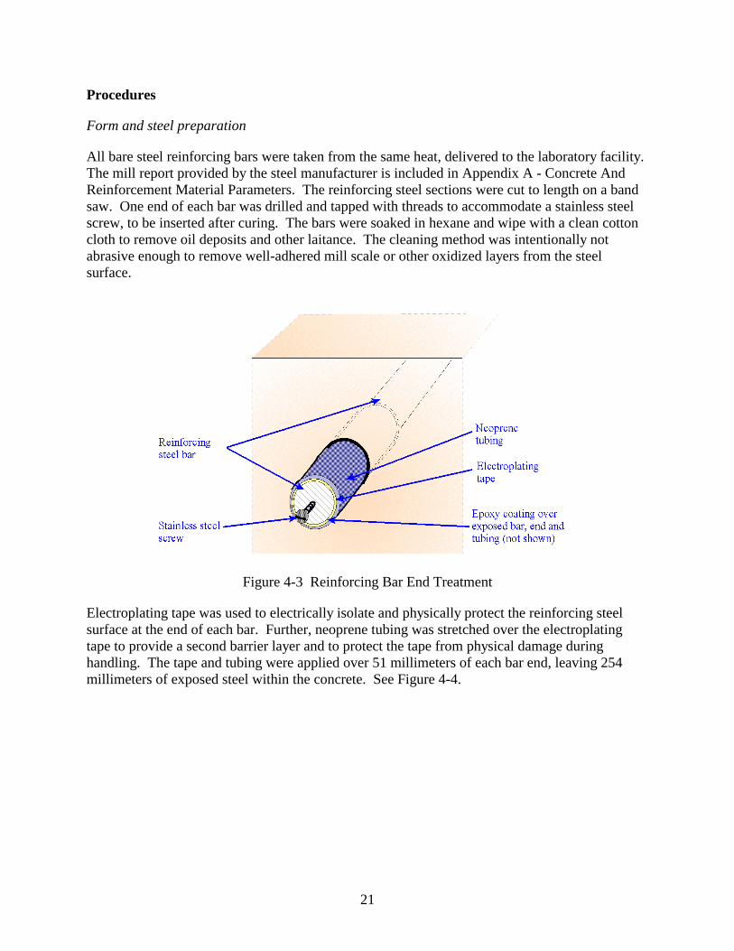
All bare steel reinforcing bars were taken from the same heat, delivered to the laboratory facility. The mill report provided by the steel manufacturer is included in Appendix A - Concrete And Reinforcement Material Parameters. The reinforcing steel sections were cut to length on a band saw. One end of each bar was drilled and tapped with threads to accommodate a stainless steel screw, to be inserted after curing. The bars were soaked in hexane and wipe with a clean cotton cloth to remove oil deposits and other laitance. The cleaning method was intentionally not abrasive enough to remove well-adhered mill scale or other oxidized layers from the steel surface.

Figure 4-3 Reinforcing Bar End Treatment

Electroplating tape was used to electrically isolate and physically protect the reinforcing steel surface at the end of each bar. Further, neoprene tubing was stretched over the electroplating tape to provide a second barrier layer and to protect the tape from physical damage during handling. The tape and tubing were applied over 51 millimeters of each bar end, leaving 254 millimeters of exposed steel within the concrete. See Figure 4-4.

22

Figure 4-4 Exposed Bar and 3LP Probe Lengths

Materials Preparation

Locally quarried limestone aggregate (from Blacksburg, Virginia), # 7/8 nominal size, was used in all of the mixtures. As indicated in batch records, the coarse aggregate had a specific gravity of 2.80 and an absorption rate of 0.85 percent. Fine aggregate was local natural sand (from Wytheville, Virginia), and with a specific gravity and absorption of 2.64 and 0.83 percent, respectively.

All aggregate was oven dried at 110 degrees Celsius for 24 hours and allowed to thoroughly cool to room temperature prior to mixing. Mixing water for each batch was adjusted to compensate for water absorption by the aggregate.

Bagged Blue Circle Type I and Type I/II cement was obtained from Marshall Concrete, Christiansburg, VA and Danville, VA. Chemical analyses of the two cements used are presented in Table A-2 of Appendix A - Concrete And Reinforcement Material Parameters. The Type I cement was used for all specimens of the Control, DCI-S, Rheocrete 222+ and FerroGard 901 series, and the first two specimens of the MCI 2005 series. The third specimen of the MCI 2005 series and the Catexol 1000 specimens contained the Type I/II cement.

Batching and Mixing

Batching, mixing and casting were performed on a single day for each of three batches in a given set. Therefore, all specimens containing a given inhibitor treatment are the same age and

23

subsequently tested at the same time. Different mixes were staggered at one-week intervals to allow staggering of subsequent specimen preparation and tests and because of the limited availability of certain equipment. Therefore, the 18 base specimens in the matrix were mixed, three per day, one day per week, for a period of approximately six weeks, until all specimens in the matrix were complete.

Material proportioning was accomplished by pre-weighing bulk materials and storing in sealed plastic buckets. All bulk materials were batched into buckets by weighing on a digital scale to the nearest 0.01 kilogram (0.02 lb). Admixtures were measured volumetrically to the nearest milliliter (for CIAs) or 0.1 milliliter (for AEA and HRWR) immediately prior to mixing. The mixtures were mixed in the laboratory using a tub-type mixer of approximately 0.06 cubic meter capacity.

One concrete prism, containing two triads, was cast for each batch. The prisms were cast in an inverted position (top bars toward the bottom) to reduce the influence of possible subsidence cracking and surface and cover irregularities, due to hand finishing, on the long term performance of the top bars. Indeed, some mixtures did exhibit minor shrinkage or subsidence cracks within the hand-finished surface over the bottom bars. These cracks were sealed with a low viscosity epoxy after curing was complete.

In addition to the prism for each batch, six cylinders, 102 millimeters diameter by 204 millimeters long, were cast for compressive strength determination in accordance with ASTM C 192-95 and ASTM C 39-96.48,49 Four specimens, 102 millimeters in diameter by 102 millimeters long, were cast for testing electrical indication of concrete’s ability to resist chloride penetration in accordance with ASTM C 1202-94.26

Finally, a 102-millimeter diameter by 204-millimeter long cylindrical specimen was cast in a standard plastic cylinder mold. The specimen contained a single Type-T thermocouple cast into the center. A polyvinyl chloride (PVC) tube, approximately 26 millimeters in diameter and 50 millimeters long was cast into the top. The specimen was used to monitor the heat of evolution of the hydration process during the first 48 hours of curing and the internal relative humidity of the concrete at the bar depth during the exposure period. A diagram of the temperature and humidity specimen is presented in Figure 4-5.

24

Figure 4-5 Temperature and Humidity Specimen

Curing

After prisms and cylinder specimens were cast, the prisms were wet-cured by covering the finished surface and forms with wet burlap and polyethylene sheet. After seven days, the forms were removed and the specimens were inverted, such that the trowel-finished surface faced down and the formed surface was at the top. The prisms were kept wet and indoors, slightly elevated off the floor, for a wet-curing period of 28 days. After the wet curing was completed, the specimens were allowed to air-cure under laboratory conditions until the specimens were approximately 60 days old.

Specimen dressing

After the air-curing period was completed, acrylic ponding dikes were secured to the top surface of the specimens with silicon sealant. Then a low viscosity epoxy coating was applied to the four sides of the prism, as well as the surface outside the ponding dikes at the top. The top surface within the dike and the bottom surface were not coated, to simulate the condition of a confined concrete deck section.

Upon completion of curing and dressing, the electroplating tape was removed from the end faces of the reinforcing bars and stainless steel screws inserted for electrical connection of the steel during subsequent monitoring. The ends of the bars were then encapsulated with the same low viscosity epoxy material as the specimen sides to preclude corrosion of the exterior portion of the reinforcing steel and to prevent the ingress of oxygen and moisture along the bar, which might induce crevice corrosion.

25

Chloride exposure

Approximately 60 days after casting, once adequate curing and environmental conditioning was complete, the specimens were subject to an initial round of electrochemical tests. After completion of the tests, weekly ponding and drying cycles were begun. The specimens were subject to ponding with a six-percent by weight solution of sodium chloride in tap water. The ponding was maintained for three and a half days and then removed, and the specimens were allowed to air dry under laboratory conditions for three and a half days. This cycle has been repeated continuously to date.

Tests

To adequately assess the condition and relative performance of the concrete specimens, it was necessary to gather data to characterize the initial condition of the specimens and then to monitor the corrosion performance of the specimens at regular intervals.

Concrete characterization tests

The following tests were performed on companion specimens cast at the time of the mixing and placement of concrete prisms in order to characterize the concrete materials in each prism.

Compressive Strength

Companion cylinders were cast at the time of concrete placement for determination of compressive strength in accordance with ASTM C 39-96.49 Six cylinders were tested for each batch of concrete. One cylinder for each batch was tested at 3 and 7 days of age, and for ages 28 and 365 days, two cylinders were tested per batch.

Heat of Hydration

Immediately after casting, each of the temperature and humidity specimens, shown in Figure 4-5, were placed in a semi-adiabatic insulated chamber. Three thermocouples were placed in the chamber, one in the center of the specimen, one at the outside surface of the plastic cylinder, and one at the inside surface of the chamber. The thermocouples were continuously monitored with a data acquisition system for 48 hours to characterize the initial rate of hydration and quantitative heat of hydration for each mixture.

After the initial 48 hours, the specimen was removed from the chamber. The temporary cap was removed, exposing the open embedded PVC tube, which was immediately plugged with a rubber stopper. An internally threaded PVC flange with a screw-in cap and rubber gasket were secured into the top of the tube with PVC cement to seal the tube but provide easy access for measurement.

Chloride Penetrability by Electrical Conductance

Specimens cast for testing Electrical Indication of Concrete’s Ability to Resist Chloride Penetration in accordance with ASTM C 1202-94 were sent to the Virginia Transportation

26

Research Council’s (VTRC) laboratory facilities in Charlottesville, Virginia.26 Two specimens for each batch were prepared and tested by VTRC personnel at approximately 28 days of age. Two additional specimens for each batch were retained in the moist curing facilities at Virginia Tech for approximately one year before being forwarded to VTRC for preparation and testing at 365 days of age.

Chloride Content

To establish the background chloride content, that amount which was present at the time of casting prior to ponding treatment, powdered samples were obtained from the fractured compressive strength cores. The powdered samples were subject to potentiometric titration in accordance with ASTM C 1152-90 to determine the acid-soluble chloride content of the concrete.50 Subsequent testing has been performed on powdered samples drilled from the top surface of select prism specimens at irregular intervals to determine the extent of chloride ion penetration into the concrete specimens.

At 24 months of ponding, sets of drilled powder samples were taken at consecutive 12.7-mm depth ranges, one set from each of the corrosion cells. Samples were drilled from the top surface into the slab and centered between the bar triads. Drill holes were sealed with epoxy-sand mortar immediately after sampling. The powdered samples were tested in each depth range to determine the chloride concentration profiles.

Corrosion assessment tests

After ponding and drying cycles were initiated, electrochemical monitoring was implemented to periodically assess the corrosion performance of each specimen. Each of the following tests has been performed on each triad within the specimen matrix on a four-week cycle.

Macro-current

The simplest electrochemical test involved measuring the macro-cell current, which is the current that is generated from corrosion activity between the top triad bar and the two bottom triad bars (see Figure 4-2). The anodic reaction (presumably) occurs at the top bar and the cathodic reaction occurs on one or both of the bottom bars.

For the ASTM G 109-type specimens, the macro-cell corrosion can be determined by measuring the potential voltage across the resistor between the top and bottom bars. If the resistance is known, then the current can be calculated according to Ohm's law. By measuring the electrical potential across the known 100-ohm resistance between the bars, the macro-cell corrosion current can be estimated.

Equation 4-1

where; V = electrical potential difference (volts) I = electrical current flow (amperes) R = electrical resistance to flow (ohms)

IRV =

27

Electrical Potential

Electrical potential for corrosion was assessed using the standard half-cell technique outlined in ASTM C 876-91.14 The method is used as an indicator of corrosion activity in localized areas of reinforcing steel by measuring the reaction potential relative to a standard copper-copper sulfate half-cell electrode (CSE), which incorporates a copper electrode in a saturated copper-sulfate electrolyte solution. The reinforcing steel acts as the second electrode and the pore solution of the concrete as the electrolyte. Connection of a volt-meter directly to the reinforcing steel and also to the CSE, which is connected to the concrete via a moist sponge, completes the cell circuit and reveals a measurable electrical potential indicative of the potential for corrosion activity.

Linear Polarization (3LP)

Linear polarization has become a popular and valuable tool in concrete corrosion science for indicating the rate at which the corrosion reaction(s) is occurring. Estimates can be made of the progress of the corrosion deterioration and the expected remaining service life of certain reinforced concrete structures based on these tests and other information about the structure.

The method employed in this research utilized the commercially available three-electrode linear polarization device (3LP), developed by K. C. Clear. A simplistic summary of the method is that the test measures the amount of outside electrical current necessary to displace the corrosion potential of the reinforcing steel by a small, but known voltage. By measuring a series of offset voltage and corresponding current values within a short range of the equilibrium potential, a linear relation can be established between corrosion potential and corrosion current, called the polarization resistance. As discussed previously, this polarization resistance, in conjunction with the Tafel, Butler-Volmer, and Stern-Geary equations, as well as Faraday’s Law, can be used to estimate the rate of metal loss due to corrosion. The 3LP method uses a Stern-Geary constant of B = 40.76, where βa = 187.5 mV per decade, and βc = 187.5 mV per decade, in converting the measured polarization resistance to an equivalent corrosion current density.

Temperature and Relative Humidity

In addition to specific electrochemical monitoring methods, ancillary monitoring was performed for temperature and relative humidity of the concrete specimens and the laboratory environment at the time of testing. Internal temperature monitoring of the concrete was achieved using a Type-T thermocouple secured to the underside of each top reinforcing bar at mid section. Temperature and relative humidity of the surrounding environment, as well as the inside of companion temperature and humidity specimens, were measured using an Omega RH 30-F combination thermocouple and relative humidity probe.

Simulated Pore Solution Immersion Test

A matrix of specimens was designed to evaluate the relative performance of three CIA’s in a simulated pore solution, under an accelerated weight loss experiment, including visual assessment of corroded steel bar surface. The test plan consists of bar sets, each bar in a separate solution container.

28

Specimens

Two hundred ten specimens were evaluated. Variables included the type and dosage of CIA, as well as solution chloride concentration.

Mild deformed steel reinforcing bars

The test specimens were #5 (16-millimeter) deformed reinforcing steel, cut to approximately 100-millimeter lengths. The reinforcing bar was bare steel, all taken from a single heat. Bar specimens were cut and labeled according to the individual bar from which the specimen was cut. Approximately twelve specimens were obtained from each bar section. Each treatment series consisted of a set of six specimens, all from the same bar.

Simulated pore solution

For this test, the bar sets were immersed in a simulated pore solution. Diamond and others performed research on the composition and proportion of pore solution in concrete, from which the solution composition for this experiment was derived.51,52 From these sources, it was established that pore solution accounts for approximately three percent by mass of a concrete, and that the primary chemical compounds in concrete pore solution may be approximated by a synthetic solution of 0.4 molar potassium hydroxide, 0.2 molar sodium hydroxide, and 0.004 molar calcium hydroxide. For purposes of solution calculations, a reasonable unit weight for concrete was established at 2,322 kilograms per cubic meter, which is substantiated by prism batch results. Simulated pore solution proportions and corresponding admixture and sodium chloride treatment dosages were based on these criteria.

Admixture and Chloride treatment matrix

The treatment matrix involved three commercially available CIA’s, DCI by W.R.Grace (DCI), Rheocrete 222+ by Master Builders (R222+), and FerroGard 901 by Sika (F901), as well as a control series. The matrix included two treatment levels, 10 liters per cubic meter and 15 liters per cubic meter, of DCI. R222+ was used at a single recommended dosage rate, 5 liters per cubic meter. Two dosage levels, 10 liters per cubic meter and 15 liters per cubic meter, were also employed for the F901 product.

The levels of chloride added to solution varied from 0.0 to 4.0 kilograms per cubic meter, corresponding to a range of 0.0 to 1.6 molar chloride in solution. Since the purported resistance to chloride ion for the recommended dosages employed varied by admixture manufacturer, a full-factorial matrix was not employed. Instead, ranges of chloride content were selected for each dosage of inhibitor to achieve data both below and just above the indicated threshold limit. A complete summary matrix is presented in Table 4-3.

29

Table 4-3 Simulated Pore Solution Immersion Test Matrix

Cl- Conc. Control Rheocrete 222+

FerroGard 901 DCI

M

0 L/m3 5 L/m3 10 L/m3 15 L/m3 10 L/m3 15 L/m3

0.00 6 6 6 - 6 - 0.20 6 6 6 6 - - 0.28 6 6 6 6 6 - 0.60 6 6 6 6 6 6 0.77 6 6 6 6 6 6 1.17 6 6 6 6 6 6 1.61

6 - 6 6 - 6

Subtotal 42 36 42 36 30 24 Total 210 Specimens

Procedures

Procedures for this phase of the research included preparation of the metal specimens and the simulated pore solutions, followed by pretreatment of the specimens in solution, addition of sodium chloride, and extended conditioning, including elevated temperature and periodic aeration.

Steel preparation

Each series consisted of six #5 (16 millimeters) deformed steel reinforcing bars, cut to approximately 100-millimeter lengths. The bars were cut on a band saw, and the ends only were polished on a ceramic grinding wheel to remove sharp edges, crevices and surface corrosion. The bars were soaked in hexane and rubbed with a clean cotton cloth to remove surface oils and excess laitance. Again, the cleaning treatment was purposely not aggressive enough to remove well-adhered mill scale or other oxidized layers. Minor traces of pre-existing corrosion products were observed on a few bars, randomly dispersed within the series. The pre-treatment condition was documented, including specimen length and weight to the nearest 0.0001 gram. Weight was measured before and after cleaning, to establish weight loss due to this procedure.

Batching

The simulated pore solution was mixed in the chemical laboratory from deionized water, reagent grade potassium hydroxide and sodium hydroxide, in pellet form, and reagent grade calcium hydroxide in powder form. All materials were batched on a weight basis. The base solution of hydroxide compounds in water was mixed first. Then, CIA, if any, was added to the solution and stirred vigorously. While continuously stirred on magnetic stirrer, the solutions were dispensed into individual, labeled 500 milliliters polypropylene containers. A varistaltic pump dispenser was used to dispense, and final adjustments were made by hand-operated pipette, to obtain 350 grams solution in each container.

30

Pretreatment

After dispensing solution, bar specimens with corresponding labels were immersed into the solution containers and the containers sealed. In each case, a single bar was placed in a single container. The containers were placed in an oven and maintained at approximately 47 degrees Celsius for a period of seven days. During pretreatment, solutions were saturated with oxygen at the start and after 3½ days.

Chloride exposure

Upon completion of the pretreatment period, reagent grade granular sodium chloride was added to solutions in accordance with the treatment matrix. The solution containers were closed and agitated briefly to ensure the sodium chloride had dissolved. Containers were returned to the oven and maintained at approximately 47 degrees Celsius for the duration of the treatment cycle.

Heat and aeration treatment

After pretreatment and chloride exposure, the solutions were maintained in the oven for an overall treatment period of 140 days (20 weeks). Twice per week the solution containers were briefly removed from the oven and pure oxygen gas (bottled) was diffused into the solutions via gas dispersion tube for one minute per specimen. The containers were immediately returned to the oven and maintained at the elevated temperature.

Tests

To evaluate the performance of the CIA’s under this test, weight loss and visual assessments were performed to provide quantitative results. The process included careful removal of excess solution precipitates from the bar surfaces, followed by forced-air drying and photographic documentation.

Weight Loss

Following the photographic documentation of bar condition immediately after drying, the specimens were weighed to the nearest 0.0001 gram and then subject to aggressive cleaning in accordance with ASTM G1-90, method C.3.5.53 Specifically, the bars were subject to cleaning in an ultrasonic bath of distilled water for five minutes, followed by immersion in acid solution for 10 minutes, and ultrasonic cleaning for an additional five minutes. The acid solution was a solution of 500 milliliters hydrochloric acid, 3.5 grams hexamethylene tetramine, and the balance deionized water to make 1 liter of solution. After cleaning, the bars were again dried with hot forced-air and weighed to the nearest 0.0001 gram. Finally, the cleaned bars were photographed and stored in dessicators to prevent further atmospheric corrosion.

Visual Assessment of Surface Corrosion

In order to provide more than just a qualitative visual analysis of the corrosion products on the surface of the bars, the photographs of both sides of the bars, prior to post-treatment cleaning, were enlarged and overlaid with a grid. A modified point-count method was employed to quantify the sectors within the grid that overlaid corroded and non-corroded sites on the bar

31

surface. By applying this method to photographs of both front and back of the bar, relative corroded surface area values were obtained. Observation of the coefficients of variation in the analysis suggests that relative comparisons between like specimens are reasonable.

Chloride content

As a check of laboratory procedures, post-treatment chloride content of the solutions was performed on randomly selected solutions. Results verified that chloride contents of the solutions were as prepared.

Electrochemical Analysis of Mild Steel in Solution

As a short-term screening method for CIA’s, electrochemical testing methods such as linear polarization resistance and electrochemical impedance spectroscopy of metal samples in simulated pore solution have been recommended. A standard screening method of this type has been proposed by ASTM sub-committee G 01.14, and is currently undergoing round robin testing. As an extension of participation in the round robin, additional cells were added to the base matrix for incorporation into the current research project. The extended test plan included increased chloride dosage levels for the DCI inhibitor and representative dosages for the two other inhibitors used in the solution testing, FerroGard 901 and Rheocrete 222+. The test matrix is presented in Table 4-4.

Table 4-4 Electrochemical Solution Test Matrix

Base* Extended Cl- (M) Inhibitor (35 ml) Cl- (M) Inhibitor (35 ml)

0.5 Control 2.0 DCI 0.5 Control 2.0 DCI 1.0 Control 3.0 DCI 1.0 Control 3.0 DCI 0.5 DCI 0.5 FerroGard 901 0.5 DCI 0.5 FerroGard 901 1.0 DCI 1.0 FerroGard 901 1.0 DCI 1.0 FerroGard 901

0.5 Rheocrete 222+ 0.5 Rheocrete 222+ 1.0 Rheocrete 222+

1.0 Rheocrete 222+ *submitted for round robin Total 20 specimens

Materials

Materials to be used for electrochemical tests in simulated pore solution were provided by W.R. Grace Corporation as part of the round robin test. Other CIA's were purchased from a local distributor.

32

Specimens

For the purposes of the round robin testing and this research project, “standard” samples designed for use in commercially available electrochemical corrosion cell kits were used. The samples were machined by Metal Samples, of Munford, Alabama (designated P/N 410). The samples were created from mild steel stock (ASTM C 1215), provided to Metal Samples by W.R. Grace Corporation. A summary of the chemical analysis for the steel specimen material is provided in Table 4-5.

Table 4-5 Chemical Analysis Report for Corrosion Cell Specimens

C1215 Steel

C (%) 0.09 N (%) 0.009

Cr (%) 0.04 S (%) 0.3

Mn (%) 0.96 Si (%) 0.02

Mo (%) 0.01 Cu (%) 0.07

P (%) 0.08 Ni (%) 0.03

Simulated Pore Solution

Unlike the long-term solution tests, the simulated pore solution for the electrochemical tests did not employ a synthetic solution of reagent hydroxide compounds. Instead, the simulated pore solution containing a CIA was extracted from slurry of Type I portland cement, deionized water and the CIA.

Equipment

In order to conduct the experiments in accordance with the proposed test procedure, specialized equipment was obtained for electrochemical analysis of the metal specimens. The major components of this system include a corrosion cell kit, computer operated potentiostat and appropriate software. Appropriate systems are available from Gamry Instruments, E,G&G, or elsewhere.

Corrosion Cell Kit

The corrosion cell kit, used to suspend the metal sample in solution and provide appropriate electrodes and connections, was a commercial unit available from Gamry Instruments. The kit includes a solution container and matching cover with ports for electrodes and purging apparatus. Also included were a graphite counter electrode rod, standard calomel electrode (SCE) reference, gas dispersion tube, working electrode specimen holder and appropriate adapters.

33

Potentiostat

The PC3/300 Potentiostat/Galvanostat/ZRA was a commercially available system of integrated circuit cards for use in IBM-PC compatible computers. The potentiostat provides the computer interface, electrical stimulation, monitoring and controls necessary to conduct a wide range of DC and AC electrochemical experiments.

Software

The CMS 100/105/300 Framework software, designed for use with the Gamry Instruments family of potentiostats, galvanostats, and ZRAs, provides the user interface and control of the PC cards and allows selection and manipulation of electrochemical techniques, as well as analysis via Microsoft Excel-based spreadsheets.

Procedures

Test procedures involved careful preparation of solution and samples, including a pretreatment period, introduction of sodium chloride into the simulated pore solution and subsequent electrochemical testing. A copy of the round robin test specification is provided in Appendix F -Electrochemical Solution Screening Test.

Specimen Preparation

The metal samples, as received, were machine finished, wrapped with a corrosion resistant paper and individually sealed in plastic. The specimens were removed from the wrappers and immersed in hexane, to remove surface oil and other contaminants. The specimen was wiped with a lint-free cloth and handled with clean latex gloves to prevent recontamination of the surface.

Solution Preparation

The slurry of 200 grams portland cement, 35 milliliters CIA, and 1 liter deionized water was batched by weight and volume, respectively, and mixed using a clean Teflon-coated magnetic stirrer. After mixing, a small amount of calcium hydroxide was added to increase the pH of the solution to about 13.0. A corrosion-inhibiting admixture was mixed into the slurry. After the slurry was stirred thoroughly, the slurry was filtered to remove all solids greater than 1.5 micrometers in diameter. The solution was air purged over night with carbon dioxide-free air, and then pretreated with the appropriate concentration of reagent grade sodium chloride. Purging continued for an additional 24 hours, and then electrochemical tests were conducted.

Tests

As indicated previously, the method employed in this phase of the project was in direct accordance with the proposed ASTM method for electrochemical analysis of mild steel in solution. This evaluation was an extension of round robin testing, which was being coordinated by ASTM subcommittee G 01.14.

34

Polarization Resistance

In accordance with the proposed test procedure, a polarization resistance test was performed in accordance with ASTM G 59-97, except that a range of –20 millivolts to +20 millivolts, relative to the equilibrium corrosion potential was used, and a polarization rate of 0.1 millivolts per second was employed.

35

5 RESULTS

Concrete Corrosion Cells

Concrete corrosion cell specimens consisted of concrete prisms, each containing two corrosion cell triads. Each prism was constructed from a separate batch, with each of three batches of a given mixture design typically prepared on the same day.

Concrete Characterization Tests

The following summarizes the results of the air content, slump, compressive strength, heat of hydration, chloride penetrability by electrical conductance and chloride tests performed to characterize the materials.

Slump, Air Content, and Compressive Strength

Slump and air content were determined at the time of batching. Compressive strength of companion cylinders was determined at 3, 7, 28, and 365 days of age for each batch. Table 5-1 presents the average result of the three batches in each series for these tests.

Table 5-1 Average Air Content, Slump, and Compressive Strength Results

Average of 3 Batches

Number of Tests

Control DCI-S Rheocrete 222+

FerroGard 901

MCI-2005 Catexol 1000

Air Content (% by volume)

3 6.4% 6.0% 6.5% 5.7% 7.0% 7.3%

Slump (mm) 3 92 62 110 92 89 83 Compressive Strength (Mpa)

3-day 3 26.0 32.8 24.2 30.5 26.8 20.5 7-day 3 30.8 42.5 29.9 38.7 36.2 25.2 28-day 6 40.8 49.2 36.5 49.9 46.0 29.9 365-day 6 52.9 61.5 46.1 61.9 57.6 37.0

The average 28-day compressive strength results ranged from 29.9 to 49.9 MPa, with no individual test below 28.5 MPa. At 365 days of age, the average compressive strength values ranged from 37.0 to 61.9 MPa, with no individual test below 36.5 MPa.

As represented in the graphical summary of average compressive strengths in Figure 5-1, the Control series compressive strengths were in the middle of the range observed. Strengths higher than that of the Control concrete were observed in the concrete containing DCI-S, FerroGard 901 and MCI-2005 at all ages.

Rheocrete 222+ and Catexol 1000 had compressive strengths less than those of the Control concrete. Indeed, the average compressive strengths observed for Catexol 1000 specimens were approximately 27 percent and 30 percent lower than the average Control concrete strengths at 28 days and 365 days of age, respectively. The average strength values of the next lowest series,

36

Rheocrete 222+, compared to Control concrete, were 11 percent lower at 28 days of age and 13 percent lower at 365 days of age.

0

10

20

30

40

50

60

70

3 7 28 365Concrete Age (Days)

Com

pres

sive

Str

engt

h (M

Pa)

Control DCI-S Rheocrete 222+ FerroGard 901 MCI-2005 Catexol 1000

Figure 5-1 Average Compressive Strengths at Various Ages

The highest concrete strengths were observed in concrete containing DCI-S and FerroGard 901. At 28 days of age, both of these mixtures had compressive strengths approximately 20 to 22 percent higher than that of the Control concrete. At 365 days of age, the average compressive strength for DCI-S and FerroGard 901 mixtures was approximately 17 percent higher than the average compressive strength of Control concrete.

It is important to note that the air content varied between batches, and more so between admixture series. Catexol 1000 and MCI 2005 mixtures possessed the highest average air contents, 7.3% and 7.0%, respectively. In contrast, Control concrete averaged 6.4% air by volume. At a given water/cement ratio and cement content, entrained air generally reduces the strength of concrete.30 Therefore, the higher air content may, in part, explain the reduction in overall compressive strength observed in Catexol 1000 specimens. However, MCI-2005 did not have a similar reduction of compressive strength. On the other hand, FerroGard 901 and DCI-S concrete had air contents of 5.7% and 6.0%, respectively, correlating with higher average compressive strengths for these series relative to Control.

Heat of Hydration

During the curing of each batch of concrete, the internal concrete temperature of companion cylinders and the ambient laboratory temperature were monitored. Typical graphs of internal

37

concrete temperature indicate a rise in temperature up to approximately 11 to 15 hours after mixing, after which concrete temperature decreased. Most concrete mixtures returned to ambient temperature within approximately 48 hours after mixing.

Results of temperature monitoring were plotted for comparison. For each series, an average temperature plot was generated for the three companion cylinders, one from each batch. The average internal concrete temperature was compared to the average ambient temperature and the area between the curves was integrated to generate a cumulative heat of hydration for each series. Table 5-2 presents the cumulative heat of hydration over periods of 24 hours and 48 hours, respectively, as well as the time and magnitude of the peak temperature and the peak difference in temperature between the specimen and the surrounding environment.

Table 5-2 Summary of Cumulative Heat of Hydration

Measured Parameter Control DCI-S R222+ F901 MCI2005 C1000

Cumulative heat - 24 hours (°C•hours) 332 350 254 272 248 302 Cumulative heat - 48 hours (°C•hours) 497 470 422 467 478 471

Peak Temp (°C) 38.2 33.9 38.6 37.7 38.3 41.1

Peak Temp Time (hours) 12.0 10.9 14.1 13.2 15.5 14.2

Peak Delta Temp* (°C) 22.0 19.2 18.6 18.2 19.1 21.1 Peak Delta Temp Time (hours) 12.6 12.3 13.2 14.9 16.7 14.0

* Peak Delta Temp – max temperature difference between internal specimen and surrounding environment

Graphical results are included in Appendix B -Heat of Hydration. For Figure B-1 through

Figure B-6, each graph represents the average internal and ambient temperature of three specimens over time, and includes a 95 percent confidence interval for the series. The cumulative heats of hydration, integrated from differential temperature data for each specimen, are presented in Figure B-7 through Figure B-12.

The series containing DCI-S showed the earliest peak of temperature, at 10.9 hours after batching. This is consistent with previous reports that calcium nitrite behaves as a hydration accelerator.36 By contrast, Rheocrete 222+ and Catexol 1000 specimens peaked at a relatively late time of 14.1 and 14.2 hours after batching. By comparison to Control concrete, which reached a peak internal hydration temperature at 12.0 hours, Rheocrete 222+ and Catexol 1000 might be judged to have a retarding effect on early cement hydration.

Chloride Penetrability by Electrical Conductance

The results of the tests, performed at 28 and 365 days of age for each series, are reported in total charge passed, in coulombs, through the concrete cylinder from one end to the other during the 6-hour test. Higher energy passed generally indicates a more permeable concrete system.

38

0

1000

2000

3000

4000

5000

6000

7000

8000

Perm

eabi

lity

(Cou

lom

bs)

Control DCI-S Rheocrete 222+ FerroGard 901 Catexol 1000 MCI -2005

denotes average value for the series

Hig

hM

oder

ate

Low

Figure 5-2 Chloride Penetrability by Electrical Conductance Results at 28 Days of Age

Weight Loss vs Corroded Surface AreaRelation within Treatment Series

-50.0%

-40.0%

-30.0%

-20.0%

-10.0%

0.0%

10.0%

20.0%

30.0%

40.0%

50.0%

-0.20% -0.15% -0.10% -0.05% 0.00% 0.05% 0.10% 0.15% 0.20%

Relative Weight Loss (%)

Rel

ativ

e Su

rfac

e A

rea

Cor

rode

d (%

)

DCI (10 L/m3) DCI (15 L/m3)

NOTE: DCI 15 L/m3 values are relative to DCI 10 L/m3 dosage and no chloride (control)

Figure 5-3 Chloride Penetrability by Electrical Conductance Results at 365 Days of Age

The average charge passed at 28 days of age ranged from 3917 coulombs to 6572 coulombs, with no individual result higher than 7357 coulombs. At 365 days of age, average charge passed

39

was significantly reduced in all mixtures, as would be expected.26 The average charge passed ranged from 2064 coulombs to 3931 coulombs, with no individual result higher than 4483 coulombs. Figure 5-2 and Figure 5-3 present individual and mean charge passed for each inhibitor sample at 28 days and 365 days of age, respectively. Tabulated results are presented in Appendix C - Chloride Penetrability by Electrical Conductance .

The method reports a coefficient of variation equal to 12.3 percent for single-operator precision, applicable in this study. Therefore, no two tests of a given inhibitor batch should differ by more than 42 percent.26 Coefficients of variation for the tests, as presented in Table C-1 and Table C-2, clearly show that the results meet this criteria for precision. The method states that a bias for the indicated chloride permeability (coulomb) values cannot be established, since the values can only be defined in relation to the test method.

Chloride Background

The background chloride contents for the mixtures ranged from 0.011 to 0.018 percent by weight of concrete sample. These values are equivalent to concentrations of 0.28 to 0.43 kg of chloride per cubic meter of concrete, based on the respective measured unit weight of each concrete mixture (nominally 2,320 kilograms per cubic meter.)

Table 5-3 Background Chloride Content

Inhibitor Series Background Cl- Concentration

(kg Cl-/m3 conc.) Control 0.43 DCI-S 0.28 Rheocrete222+ 0.42 FerroGard 901 0.32 MCI - 2005 0.32 Catexol 1000 0.29 Overall Mean 0.34 Standard Deviation 0.07 Coefficient of Variation 20.6%

Chloride content

After 24 months of exposure, powdered concrete samples were obtained from the prism specimens at five equal, 13-millimeter increments, ranging from approximately 5 millimeters to 70 millimeters of depth from the top surface. The resulting chloride contents were corrected by subtracting the mean background chloride content for the mixtures, as determined from companion cylinders after placement. Chloride content profiles, as a function of depth, were generated. The profiles are presented graphically in Appendix D - Chloride Profiles.

Table 5-4 presents the mean acid-soluble chloride concentrations (not corrected for background) versus depth for each set of prism specimens and the associated standard deviation and coefficient of variance.

40

After 24 months, chloride concentrations at 38-mm depth and below for most specimens was similar to that of the background for the mixtures prior to ponding. Therefore, only chloride concentrations above 38-mm depth were considered for comparison of diffusion behavior. Since significant chloride diffusion did not appear to have occurred below this depth after two years exposure for most series, there were insufficient data points in each chloride concentration profile to effectively calculate estimate diffusion constant, Dc, for each sample. Therefore, direct contrasts were made between the chloride contents of Control and each inhibitor at 13 mm and 25 mm depths.

Table 5-4 Descriptive Statistics of Chloride Content by Depth and Inhibitor

Depth Inhibitor Average* StDev CV Range Treatment (kg/m3) (kg/m3) (kg/m3) 13 mm Control 6.91 0.61 9%

DCI-S 5.69 0.71 12% Rheocrete 222+ 3.13 0.37 12% FerroGard 901 5.71 0.83 15% MCI-2005 4.13 2.09 51% Catexol 1000 4.78 0.70 15%

25 mm Control 3.78 0.94 25% DCI-S 2.99 0.49 16% Rheocrete 222+ 0.77 0.15 19% FerroGard 901 1.54 0.38 25% MCI-2005 1.43 0.87 61% Catexol 1000 1.34 0.15 11%

38 mm Control 1.02 0.35 34% DCI-S 0.80 0.18 23% Rheocrete 222+ 0.29 0.02 7% FerroGard 901 0.38 0.05 13% MCI-2005 0.42 0.08 19% Catexol 1000 0.37 0.09 24%

*Note: Not corrected for background chloride content

For small sample sizes from a normally distributed population of unknown variance, Student’s t−distribution provides a more reasonable approximation to the distribution than the normal (Guassian) distribution.54 As the sample size increases, the t–distribution approaches that of the normal distribution. However, for each depth, only three samples were available for each inhibitor treatment. Even under the t-test, three samples are insufficient to accurately gage variation within a treatment series.

Therefore, the variation in chloride concentration was evaluated using a general randomized block design, where each depth was considered a block, and comparisons of chloride treatments were made from each inhibitor to the Control over a range of depths. This method allowed the use of the combined samples from the 13-mm and 25-mm depth ranges over which it is expected

41

that diffusion might have occurred. The resultant comparisons of chloride content of each inhibitor to the Control series are presented in Table 5-5.

Table 5-5 Comparison of Chloride Concentration by Inhibitor

Contrast Compared to Control

p-value

DCI-S 0.0647 R222+ <.0001 F901 0.003 MCI-2005 <.0001 C1000 0.0002

Chloride concentrations at the steel depth in Control specimens averaged the highest of all the series. Contrast of chloride contents in the range of 13 mm to 25 mm for each inhibitor revealed a reduction of chloride, and hence diffusion, for all inhibitors relative to Control. Calculated p-values for each comparison are listed in the right column of Table 5-5. These values may be used to assess the significance of the test (the lower the p-value, the more significant the difference.) Comparison of these values to the significance level of α=0.05 indicate differences in chloride concentration between Control and each of the inhibitors, except DCI-S, which would be considered similar to Control at this significance level. Generally, each of the inhibitors showed a positive influence with regard to chloride diffusion during the first two years of exposure, as compared to Control concrete. A comparison of chloride penetrability by electrical conductance, compressive strength and diffused chloride results will be discussed in Chapter 6.

Corrosion Assessment Tests

Electrochemical tests included measurement of macro-cell corrosion current, electrical potential, linear polarization, temperature and relative humidity. Electrochemical measurements for specimens did not indicate active corrosion up to the time of chloride sampling with the exception of two Control cells in a single specimen. Elevation in electrical potential and macro-cell current was noted in at least one cell of each of the three Control specimens. However, 3LP results only indicated significant corrosion rates in the two cells of the third Control specimen.

Macro-cell Corrosion Current

Macro-cell corrosion current was documented in monthly tests for a period of two years. Figure 5-4 presents an example summary of the macro-cell corrosion current measured over a period of two years.

42

MCB-C (Control)

0

10

20

30

40

50

60

70

80

90

100

110

120

130

140

150

2 4 6 8 10 12 14 16 18 20 22 24Specimen Age (months)

Mac

ro C

urre

nt ( µ µµµ

A)

Average (1)Average (2)Average (3)

Threshold

Begin ponding after initial tests

Macro Corrosion Current over Time

Cell 3b cracked Cell 3a cracked

Figure 5-4 Typical Summary of Macro-Cell Corrosion Readings – Control Series

Note that the values for Specimen 3 of the Control series are significantly higher than in the others. Specimen 3 was the first specimen to enter corrosion, at an unusually early age, approximately four months after casting. Specimens 1 and 2 of the Control series began to exhibit some signs of corrosion activity at 12 and 14 months, respectively. The values shown in Figure 5-4 are averages of the two cells within a single specimen. Figure E-1 through Figure E-6 of Appendix E - Concrete Electrochemical Tests contain individual graphs of macro-cell corrosion current for each of three specimens in a given series, with a separate line for each cell.

It has already been noted that both the "a" (left) and "b" (right) cells within Control Specimen 3 entered into corrosion activity at an exceptionally early age. Macro-cell corrosion activity was observed in the "a" cell of Control Specimen 1 at approximately 16 months of age, but corrosion activity has not remained consistently above the threshold level. Cell "b" of Control Specimen 2 initiated macro cell corrosion at approximately 13 months of age, and has continued above the threshold level since that time. Hence, three of the six cells within the control series have initiated corrosion within the first two years.

Macro-cell corrosion measurements for the DCI-S, Rheocrete 222+, FerroGard 901, Catexol 1000 and MCI 2005 series revealed no significant macro-cell corrosion during the initial two-year treatment.

43

Electric Potential

Prior to corrosion initiation, the corrosion potential readings for control specimens, as with most other series, generally fluctuated between -100 and -150 millivolts CSE.

Cell "a" of Control Specimen 1 reflected a more negative trend in potential at approximately 16 months of age, however, potential readings remained less negative than the threshold level, -350 millivolts CSE, which indicates high probability of corrosion, according to ASTM C 876-91. Cell "b" of Control Specimen 2 displayed more negative corrosion potential readings at approximately 13 months of age, and fluctuated near the high probability of corrosion potential through the end of the 24-month evaluation period. As indicated previously, corrosion potential of both cells of Control Specimen 3 became more negative than the high probability of corrosion threshold at approximately four months of age. Potentials for the cells remained high above the high probability of corrosion threshold for the remainder of the evaluation period.

MCB-C (Control)

0

100

200

300

400

500

600

700

2 4 6 8 10 12 14 16 18 20 22 24

Specimen Age (months)

Ref

eren

ce P

oten

tial (

-mV

CSE

)

Average (1)Average (2)Average (3)

High probability of Corrosion

Begin ponding after initial tests

Electrical Potential

Cell 3b cracked Cell 3a cracked

Figure 5-5 Typical Summary of Electric Corrosion Potential – Control Series

Figure 5-5 summarizes electric potential activity of Control specimens. Detailed summary plots of electric potential for each specimen, grouped by series, are included in Figure E-7 through Figure E-12 in Appendix E - Concrete Electrochemical Tests.

Electric corrosion potential readings for the DCI-S, Rheocrete 222+, FerroGard 901, Catexol 1000 and MCI 2005 series generally remained more positive than -200 millivolts CSE, which

44

indicates a low probability of active corrosion. In fact, electric corrosion potential readings for Rheocrete 222+ series remained well below the -100 millivolts CSE level.

Linear Polarization

Linear polarization tests were conducted on a monthly basis for each cell of each series, to assess the rate of localized corrosion of the surface of the top bar each cell.

A significant point of debate with regard to the employment of linear polarization, especially with regard to field structures, is the length of the steel polarized during the test. A common evaluation procedure involves conversion of measured current data into corrosion current density, and then weight loss can be estimated. In order to conduct the analysis, an area of polarized bar must be assumed. Commonly, the length of the 3LP probe is considered as the length over which the bar is polarized. However, the dispersion of induced current from the counter electrode in the probe is likely greater than the length of the electrode. Researchers have attempted to manufacture and investigate devices that restrict the dispersion of induced current, via a guard ring device.55 Mixed results have been reported.24,56

For the purposes of this study, the area of bar exposed to polarization was assumed to be the surface area of a cylindrical specimen of nominal bar diameter (neglecting deformations) along the length of the counter electrode (181 mm). Since the study involves specimens of identical geometry and all measured with the same probe, all comparisons are relative, and absolute corrosion current density is not a factor in the evaluation. The polarized length could alternatively have been considered the exposed length, being that length within the specimen which is in direct contact with concrete and not covered by electroplating tape and neoprene (254 mm), as shown in Figure 4-4.

Figure 5-6 presents an example summary of linear polarization current density results, which displays the average of two cells for each of the three control specimens. The figure displays a significant increase in corrosion activity in Control Specimen 3 at approximately four months of age, corresponding to the results found in potential and macro-cell corrosion readings.

Linear polarization current density readings for the remaining control cells remained below the indicated threshold limit for active corrosion the remainder of the 24-month exposure period. However, cell "b" of Control Specimen 2 showed in the increase in corrosion at age 13 months, which continued to rise through the remainder of the exposure period.

All specimens demonstrated a slight elevated linear polarization corrosion current density reading during the initial two months of exposure, which is probably related to the formation of the passive layer at the steel surface. Subsequently all specimens of the DCI-S, Rheocrete 222+, FerroGard 901, Catexol 1000, and MCI 2005 series maintained corrosion current density rates of less than 0.5 micro-amps per square centimeter, indicating no significant corrosion the remainder of the 24 month exposure period. Detailed summary plots of linear polarization current density for each specimen, grouped by series, are included in Figure E-13 through Figure E-18 in Appendix E - Concrete Electrochemical Tests.

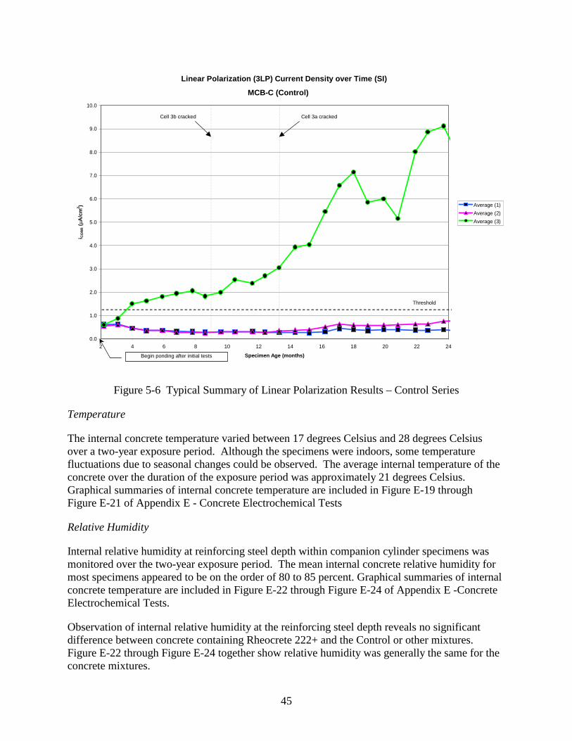
45

MCB-C (Control)

0.0

1.0

2.0

3.0

4.0

5.0

6.0

7.0

8.0

9.0

10.0

2 4 6 8 10 12 14 16 18 20 22 24

Specimen Age (months)

i CO

RR ( µ

A/c

m2 ) Average (1)

Average (2)Average (3)

Begin ponding after initial tests

Threshold

Linear Polarization (3LP) Current Density over Time (SI)

Cell 3b cracked Cell 3a cracked

Figure 5-6 Typical Summary of Linear Polarization Results – Control Series

Temperature

The internal concrete temperature varied between 17 degrees Celsius and 28 degrees Celsius over a two-year exposure period. Although the specimens were indoors, some temperature fluctuations due to seasonal changes could be observed. The average internal temperature of the concrete over the duration of the exposure period was approximately 21 degrees Celsius. Graphical summaries of internal concrete temperature are included in Figure E-19 through Figure E-21 of Appendix E - Concrete Electrochemical Tests

Relative Humidity

Internal relative humidity at reinforcing steel depth within companion cylinder specimens was monitored over the two-year exposure period. The mean internal concrete relative humidity for most specimens appeared to be on the order of 80 to 85 percent. Graphical summaries of internal concrete temperature are included in Figure E-22 through Figure E-24 of Appendix E -Concrete Electrochemical Tests.

Observation of internal relative humidity at the reinforcing steel depth reveals no significant difference between concrete containing Rheocrete 222+ and the Control or other mixtures. Figure E-22 through Figure E-24 together show relative humidity was generally the same for the concrete mixtures.

46

Occasionally, relative humidity readings in excess of 100 percent were observed. This is likely the result of slight variations in temperature between the probe and the specimen at the time of measurement, which caused condensation on the surface of the probe. However, relative humidity readings for the FerroGard 901 series remained in the mid-90’s, with a significant variation between specimens. The consistent measurement above 100 percent of one particular specimen is not likely to be the result of temperature differentials as mentioned previously. It is possible in the case of this specimen, however, that moisture from ponding found a direct path into the humidity chamber. In any case, it is reasonable to surmise that this concrete, under cyclic ponding, retained internal relative humidity on the order of 90 percent or more.

Simulated Pore Solution Immersion Test

Prior to exposure, the individual reinforcing steel bars were measured for length, and weighed to provide a benchmark for comparison after exposure. Subsequent to exposure, the specimens were cleaned and re-weighed. The relative percent of each bar surface exhibiting corrosion was also estimated by visual analysis. Descriptive statistics regarding the relative weight loss and relative corroded surface area within each series, as explained in the following paragraphs, is presented in Table 5-6. Note that a negative value for mean weight loss under Column 3 of this table simply indicates that the group lost less weight on average than the no-chloride exposure set to which it was compared. Contrasts of weight loss and corroded surface area for each inhibitor against the Control, based on a complete randomized experimental design, are summarized in Table 5-7. Contrast p-values less than α=0.05 were considered to indicate statistically significant differences.

Comparisons were also made between the Control series and each inhibitor/dosage series by plotting the means and 95% confidence intervals for relative weight loss and relative corroded surface area, assuming the results were normally distributed. The comparison indicates no difference if the 95% confidence intervals overlap. If the 95% confidence intervals do not overlap, then a statistically significant difference is indicated.

A comment on precision for the methods is warranted. Coefficients of variation for both relative weight loss and relative corroded surface area were very high in some cases, as shown in Table 5-6. The weight loss evaluation was made by comparison of pre-test and post-test weights, each measured to the nearest 0.0001 gram. Typically, observed weight losses were on the order of 1 gram for a 140-gram specimen. This would suggest a considerable precision for the test. However, comparisons must be made on a relative weight loss basis, since the post-treatment cleaning process will inevitably remove the mill scale (oxidized steel) and some base metal, regardless of the presence of corrosion.

47

Table 5-6 Descriptive Statistics of Relative Weight Loss and Relative Surface Corrosion Weight Loss CorrArea Mean StDev CV Mean StDev CV

0.20 molar Cl- Control 0 L/m3 0.013% 0.018% 142% 3.0% 4.6% 154% Rheocrete 222+ 5 L/m3 0.025% 0.015% 60% 6.5% 2.4% 37% FerroGard 901 10 L/m3 -0.065% 0.023% 36% 11.2% 2.0% 18% FerroGard 901 15 L/m3 -0.027% 0.020% 72% 14.2% 4.3% 30% DCI 10 L/m3 - - - - - - DCI 15 L/m3 - - - - - -

0.28 molar Cl- Control 0 L/m3 0.009% 0.035% 371% 1.9% 2.9% 155% Rheocrete 222+ 5 L/m3 -0.023% 0.013% 57% 24.6% 4.9% 20% FerroGard 901 10 L/m3 -0.061% 0.017% 28% 13.9% 2.3% 16% FerroGard 901 15 L/m3 -0.027% 0.020% 72% 20.8% 5.0% 24% DCI 10 L/m3 -0.042% 0.010% 25% -1.6% 1.5% 92% DCI 15 L/m3 - - - - - -

0.60 molar Cl- Control 0 L/m3 0.027% 0.017% 63% 14.9% 3.2% 21% Rheocrete 222+ 5 L/m3 -0.039% 0.024% 60% 24.9% 4.2% 17% FerroGard 901 10 L/m3 0.063% 0.016% 25% 11.8% 5.4% 46% FerroGard 901 15 L/m3 0.088% 0.034% 39% 17.7% 2.3% 13% DCI 10 L/m3 -0.029% 0.089% 311% 10.2% 1.8% 18% DCI 15 L/m3 -0.150% 0.078% 52% 9.9% 2.8% 28%

0.77 molar Cl- Control 0 L/m3 0.041% 0.019% 46% 21.5% 3.0% 14% Rheocrete 222+ 5 L/m3 0.066% 0.020% 31% 22.6% 8.0% 35% FerroGard 901 10 L/m3 0.065% 0.014% 22% 19.8% 4.8% 24% FerroGard 901 15 L/m3 0.099% 0.027% 27% 26.8% 4.8% 18% DCI 10 L/m3 0.143% 0.042% 29% 9.3% 2.8% 30% DCI 15 L/m3 -0.078% 0.016% 20% 13.4% 3.2% 24%

1.17 molar Cl- Control 0 L/m3 0.121% 0.029% 24% 19.9% 3.1% 16% Rheocrete 222+ 5 L/m3 0.067% 0.034% 51% 24.1% 3.8% 16% FerroGard 901 10 L/m3 -0.013% 0.014% 105% 25.3% 1.7% 7% FerroGard 901 15 L/m3 0.139% 0.012% 9% 24.1% 3.3% 14% DCI 10 L/m3 0.178% 0.031% 17% 9.2% 5.3% 57% DCI 15 L/m3 0.116% 0.016% 14% 20.8% 3.7% 18%

1.61 molar Cl- Control 0 L/m3 0.126% 0.050% 40% 22.8% 4.6% 20% Rheocrete 222+ 5 L/m3 - - - - - - FerroGard 901 10 L/m3 -0.002% 0.014% 896% 25.2% 5.0% 20% FerroGard 901 15 L/m3 0.172% 0.024% 14% 9.0% 5.4% 60% DCI 10 L/m3 - - - - - - DCI 15 L/m3 0.147% 0.018% 12% 21.5% 1.8% 9%

48

Table 5-7 Contrast of Inhibitors to Control – Weight Loss and Surface Corrosion

Contrast to Control Weight

Loss Corroded

Surface Area Weight

Loss Corroded

Surface Area

0.20 Molar Cl- p-value p-value 0.77 Molar Cl- p-value p-value R222+@5 L/m3 0.3015 0.0774 R222+@5 L/m3 0.0893 0.6975 F901@10L/m3 <.0001 0.0005 F901@10L/m3 0.1004 0.5348 F901@15L/m3 0.0017 <.0001 F901@15L/m3 0.0003 0.0652 DCI@10L/m3 - - DCI@10L/m3 <.0001 0.0001 DCI@15L/m3 - - DCI@15L/m3 <.0001 0.0061 0.28 Molar Cl- p-value p-value 1.17 Molar Cl- p-value p-value R222+@5 L/m3 0.0131 <.0001 R222+@5 L/m3 0.0006 0.0513 F901@10L/m3 <.0001 <.0001 F901@10L/m3 <.0001 0.0151 F901@15L/m3 0.0055 <.0001 F901@15L/m3 0.2178 0.0513 DCI@10L/m3 0.0002 0.1056 DCI@10L/m3 0.0003 <.0001 DCI@15L/m3 - - DCI@15L/m3 0.7423 0.6533

0.60 Molar Cl- p-value p-value 1.61 Molar Cl- p-value p-value R222+@5 L/m3 0.0353 <.0001 R222+@5 L/m3 - - F901@10L/m3 0.2375 0.1362 F901@10L/m3 <.0001 0.3451 F901@15L/m3 0.0493 0.1649 F901@15L/m3 0.0153 <.0001 DCI@10L/m3 0.0752 0.0265 DCI@10L/m3 - - DCI@15L/m3 <.0001 0.0185 DCI@15L/m3 0.2497 0.6183

It is known that as temperature increases in an oxygen-rich, high-pH environment, there comes a point where spontaneous corrosion of iron will occur, even in the absence of chloride.57 This is representative of the increasing area of stability of HFeO2

- ions, where alternative reactions for dissolution of iron are possible.58 To address the severity of the exposure regime for this test, specific comparison between blanks and chloride-free solutions was made. Statistical similarity was established between weight loss of blank specimens (subject to cleaning, but not immersed in pore solution and not subject to the exposure regime) and the weight loss of no-chloride pore solution specimens (subject to control and inhibitor-containing solutions with no chloride added under the exposure regime). Therefore, the accelerated exposure regime, at 47 degrees Celsius and receiving biweekly oxygen saturation, was not excessive, in that no measurable corrosion-related weight loss occurred in solution in the absence of admixed chloride. Furthermore, a study by Liu indicates internal concrete temperatures at the reinforcing steel depth of full-scale specimens in Virginia during summer months may be as high as 43.3 degrees Celsius (110°F).15

For weight loss between corroded and uncorroded specimens, the average difference was generally on the order of 0.08 grams. Therefore, the actual weight differences upon which the data is being evaluated are small in comparison to the overall weight losses measured. However, consider that, with weight measurements to the nearest 0.0001 gram, an average corrosion-related weight loss of 0.08 grams would still give precision of 0.0001/0.08 = 0.125%. Thus, the precision of this method is reasonable.

49

The visual assessment of corroded surface area involved classification of approximately 420 points over the surface of each specimen. Therefore, the ultimate precision of this method can be no greater than 1/420*100 = 0.24% for a specimen. Again the surface area values must be compared on a relative basis, by subtracting the values for no-chloride specimens. On this basis, the overall average corroded surface area was 39.3%, while that of no-chloride specimens (including inhibitor series) was 28.8%, which would be considered the benchmark for comparison. Unlike the weight loss determinations, surface area analysis did not include the subtraction of pre-treatment measurements. The pre-treatment cleaning method, involving hexane, intentionally did not remove all existing surface oxidation products. Therefore, the seemingly high average corroded surface of no-chloride specimens does not indicate an overly aggressive exposure regime, but simply the presence of pre-test oxidation products. All comparisons are made on a relative basis between specimens from the same heat and handled in the same manner.

Weight Loss

Individual bar weights were subtracted from pre-exposure weight to obtain a quantitative weight loss due to exposure. Absolute weight loss (mass loss from pre-exposure to post-treatment cleaning) was converted to percentage weight loss (absolute weight loss divided by the pre-exposure weight) for comparison. The mean percentage weight loss, for each group of six bars was obtained, along with standard deviation and a 95 percent confidence interval for each group. The relative weight loss for each group of bars was compared within series by subtracting the average percent weight loss of the group containing no chloride for a given series from the average percent weight loss of each other group of the same series. Therefore, the no-chloride group within a treatment series was the datum for comparison.

Figure 5-7 is a plot comparing relative weight loss between Rheocrete 222+ and Control series. By definition, the within series comparison equates no-chloride groups for each series, setting them each at 0% relative weight loss.

First observe the response of the Control series. Relation of relative weight loss to chloride for the Control series was reasonably linear as might be expected. Relative weight loss is near constant up to 0.28 molar chloride, which is approximately equivalent to 0.7 kg of chloride per cubic meter of concrete. Then the weight loss increases, as the chloride concentration increases, supporting previous assumptions concerning the nominal chloride concentration threshold for reinforcement corrosion in untreated concrete.

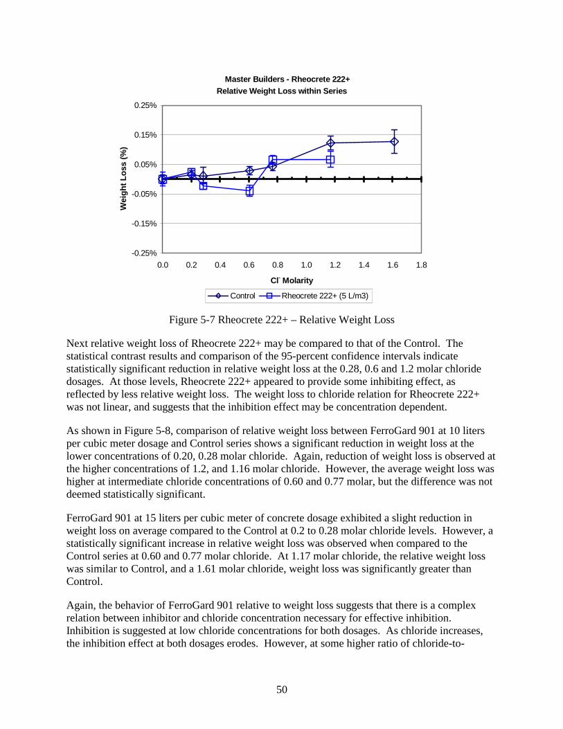
50

Relative Weight Loss within Series

-0.25%

-0.15%

-0.05%

0.05%

0.15%

0.25%

0.0 0.2 0.4 0.6 0.8 1.0 1.2 1.4 1.6 1.8

Cl- Molarity

Wei

ght L

oss

(%)

Control Rheocrete 222+ (5 L/m3)

Master Builders - Rheocrete 222+

Figure 5-7 Rheocrete 222+ – Relative Weight Loss

Next relative weight loss of Rheocrete 222+ may be compared to that of the Control. The statistical contrast results and comparison of the 95-percent confidence intervals indicate statistically significant reduction in relative weight loss at the 0.28, 0.6 and 1.2 molar chloride dosages. At those levels, Rheocrete 222+ appeared to provide some inhibiting effect, as reflected by less relative weight loss. The weight loss to chloride relation for Rheocrete 222+ was not linear, and suggests that the inhibition effect may be concentration dependent.

As shown in Figure 5-8, comparison of relative weight loss between FerroGard 901 at 10 liters per cubic meter dosage and Control series shows a significant reduction in weight loss at the lower concentrations of 0.20, 0.28 molar chloride. Again, reduction of weight loss is observed at the higher concentrations of 1.2, and 1.16 molar chloride. However, the average weight loss was higher at intermediate chloride concentrations of 0.60 and 0.77 molar, but the difference was not deemed statistically significant.

FerroGard 901 at 15 liters per cubic meter of concrete dosage exhibited a slight reduction in weight loss on average compared to the Control at 0.2 to 0.28 molar chloride levels. However, a statistically significant increase in relative weight loss was observed when compared to the Control series at 0.60 and 0.77 molar chloride. At 1.17 molar chloride, the relative weight loss was similar to Control, and a 1.61 molar chloride, weight loss was significantly greater than Control.

Again, the behavior of FerroGard 901 relative to weight loss suggests that there is a complex relation between inhibitor and chloride concentration necessary for effective inhibition. Inhibition is suggested at low chloride concentrations for both dosages. As chloride increases, the inhibition effect at both dosages erodes. However, at some higher ratio of chloride-to-

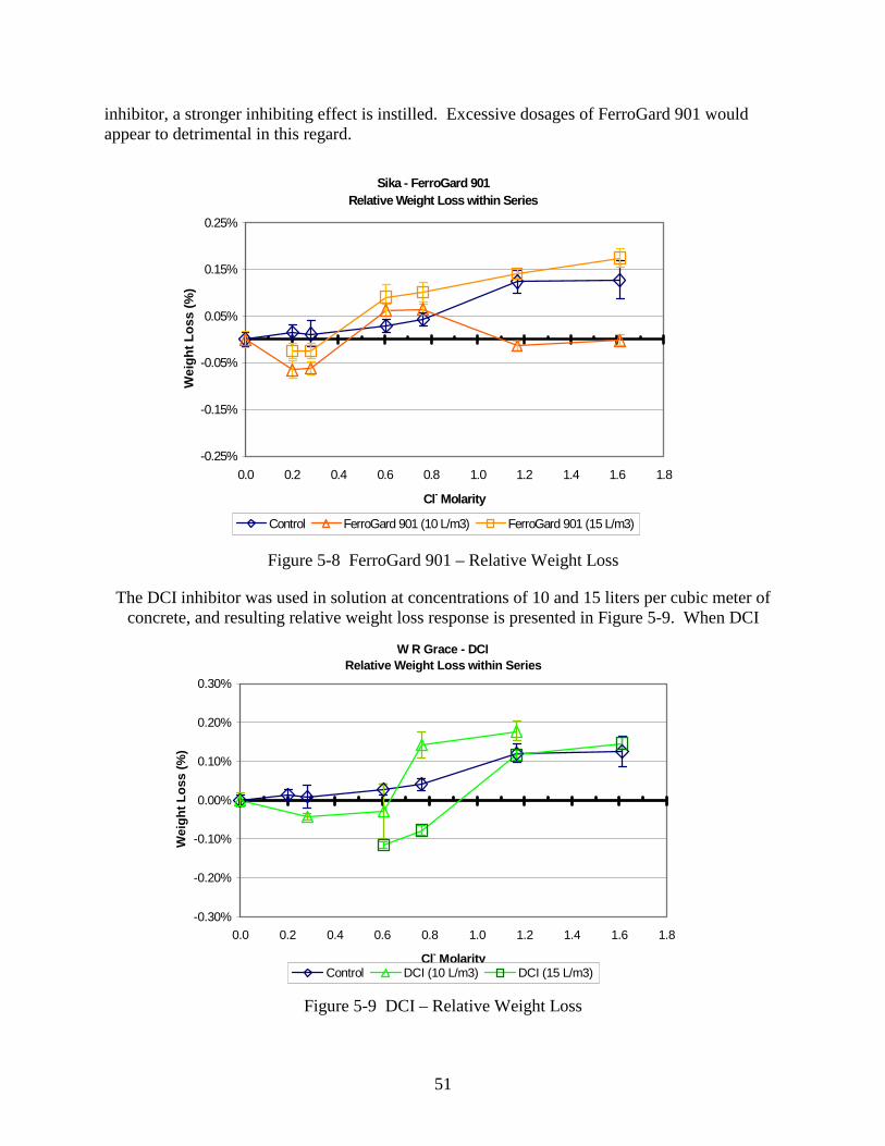
51

inhibitor, a stronger inhibiting effect is instilled. Excessive dosages of FerroGard 901 would appear to detrimental in this regard.

Relative Weight Loss within Series

-0.25%

-0.15%

-0.05%

0.05%

0.15%

0.25%

0.0 0.2 0.4 0.6 0.8 1.0 1.2 1.4 1.6 1.8

Cl- Molarity

Wei

ght L

oss

(%)

Control FerroGard 901 (10 L/m3) FerroGard 901 (15 L/m3)

Sika - FerroGard 901

Figure 5-8 FerroGard 901 – Relative Weight Loss

The DCI inhibitor was used in solution at concentrations of 10 and 15 liters per cubic meter of concrete, and resulting relative weight loss response is presented in Figure 5-9. When DCI

Relative Weight Loss within Series

-0.30%

-0.20%

-0.10%

0.00%

0.10%

0.20%

0.30%

0.0 0.2 0.4 0.6 0.8 1.0 1.2 1.4 1.6 1.8

Cl- Molarity

Wei

ght L

oss

(%)

Control DCI (10 L/m3) DCI (15 L/m3)

W R Grace - DCI

Figure 5-9 DCI – Relative Weight Loss

52

treated series were compared to Control on the basis of relative weight loss, DCI, at 10 liters per cubic meter dosage, did not appear to inhibit weight loss above approximately 0.7 molar chloride concentration. This concentration would be similar to 1.8 kg of chloride per cubic meter of concrete. In fact, a statistically significant increase in weight loss was shown at higher chloride concentrations.

DCI at 15 liters per cubic meter dosage showed a strong inhibiting effect below 1.2 molar chloride concentrations. At or above concentrations of 1.2 molar chloride, no significant difference in weight loss relative to Control. Thus, the effectiveness of the inhibitor can be reasonably concluded to be directly proportional to the chloride-to-inhibitor ratio. The increase in weight loss after inhibition effects are overwhelmed by available chloride is consistent with previous reports concerning anodic inhibitors in general and nitrite inhibitors specifically.37,36 Thus, adequate dosage appears crucial to performance.

Visual Assessment of Surface Corrosion

Visual assessment of each of the bars in the condition after treatment but prior to cleaning was used to estimate the surface area corroded during treatment. A numerical percentage of corroded surface area was determined for each of two sides of each bar. The total percent area for each of six specimens was averaged to provide an average surface area corroded per group and associated standard deviation and 95 percent confidence interval. As with the weight loss measurements, average corroded surface area for each group of bars was compared within series by subtracting the average corroded surface area of the group containing no chloride from the average corroded surface area of each other group of the series.

Relative Corroded Surface AreaControl and Rheocrete 222+ Compared Within Series

-5%

0%

5%

10%

15%

20%

25%

30%

0.00 0.20 0.40 0.60 0.80 1.00 1.20 1.40 1.60 1.80

Chloride Content (Molar Cl-)

Surf

ace

Are

a C

orro

ded R

elat

ive

to C

ontr

ol (

%)

Control Rheocrete 222+ (5L/m3) Figure 5-10 Rheocrete 222+ – Relative Corroded Surface Area

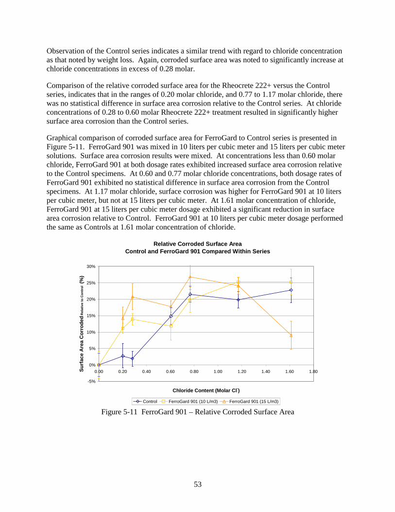
53

Observation of the Control series indicates a similar trend with regard to chloride concentration as that noted by weight loss. Again, corroded surface area was noted to significantly increase at chloride concentrations in excess of 0.28 molar.

Comparison of the relative corroded surface area for the Rheocrete 222+ versus the Control series, indicates that in the ranges of 0.20 molar chloride, and 0.77 to 1.17 molar chloride, there was no statistical difference in surface area corrosion relative to the Control series. At chloride concentrations of 0.28 to 0.60 molar Rheocrete 222+ treatment resulted in significantly higher surface area corrosion than the Control series.

Graphical comparison of corroded surface area for FerroGard to Control series is presented in Figure 5-11. FerroGard 901 was mixed in 10 liters per cubic meter and 15 liters per cubic meter solutions. Surface area corrosion results were mixed. At concentrations less than 0.60 molar chloride, FerroGard 901 at both dosage rates exhibited increased surface area corrosion relative to the Control specimens. At 0.60 and 0.77 molar chloride concentrations, both dosage rates of FerroGard 901 exhibited no statistical difference in surface area corrosion from the Control specimens. At 1.17 molar chloride, surface corrosion was higher for FerroGard 901 at 10 liters per cubic meter, but not at 15 liters per cubic meter. At 1.61 molar concentration of chloride, FerroGard 901 at 15 liters per cubic meter dosage exhibited a significant reduction in surface area corrosion relative to Control. FerroGard 901 at 10 liters per cubic meter dosage performed the same as Controls at 1.61 molar concentration of chloride.

Relative Corroded Surface AreaControl and FerroGard 901 Compared Within Series

-5%

0%

5%

10%

15%

20%

25%

30%

0.00 0.20 0.40 0.60 0.80 1.00 1.20 1.40 1.60 1.80

Chloride Content (Molar Cl-)

Surf

ace

Are

a C

orro

ded

Rel

ativ

e to

Con

trol

(%

)

Control FerroGard 901 (10 L/m3) FerroGard 901 (15 L/m3) Figure 5-11 FerroGard 901 – Relative Corroded Surface Area

54

Relative Corroded Surface AreaControl and DCI Compared Within Series

-5%

0%

5%

10%

15%

20%

25%

30%

0.00 0.20 0.40 0.60 0.80 1.00 1.20 1.40 1.60 1.80

Chloride Content (Molar Cl-)

Surf

ace

Are

a C

orro

ded

Rel

ativ

e to

Con

trol

(%

)

Control DCI (10 L/m3) DCI (15 L/m3) Figure 5-12 DCI – Relative Corroded Surface Area

The relation of corroded surface area to chloride and inhibitor contents for FerroGard 901 is not readily apparent. Beneficial results with regard to surface area corroded were only observed in the series containing both the highest inhibitor dosage and the highest chloride exposure. At lower chloride exposures, the percentage of surface area under corrosion appeared to be greater, as a whole, than the Control series.

Comparison of DCI inhibitor specimens to the Control series is presented in Figure 5-12. Surface area corrosion for DCI specimens remains generally lower than that of Controls, except for the 15 liters per cubic meter dosage at 1.17 molar chloride concentration or higher.

The only statistically significant reduction in corroded surface area for DCI was observed at 0.60 and 0.77 molar concentrations for both dosage levels, and 1.17 molar chloride concentrations for the 10 liters per cubic meter dosage of DCI. All other groups were comparable in surface area corrosion to those of the Control series.

Graphical comparisons of weight loss versus surface area corrosion for each series of solution tests will be discussed in Chapter 6.

Screening Method – Electrochemical Analysis of Mild Steel in Solution

A series of experiments were performed to test a potential screening method for corrosion inhibiting admixtures for concrete. The screening method involves immersion of a small metal test sample into a cement slurry solution containing the admixture product. The experiment involved an electrochemical cell in which the sample functions as the working electrode, the solution as the electrolyte. A single test typically require approximately 21/2 days to complete,

55

including mixing the solution, immersion of the specimen and pretreatment for 24 hours, exposure to chloride for 24 hours, and electrochemical testing.

Tests

After pretreatment and exposure to chloride at predetermined levels, polarization resistance (PR) tests were performed using a potentiostat in accordance with the round robin evaluation specifications.

Polarization Resistance

During the polarization resistance test, appropriate current was applied to the system to cause a potential sweep from 20 millivolts below the equilibrium corrosion potential to 20 millivolts above the equilibrium corrosion potential of the cell. The necessary current was plotted against the potential response and the slope of the resulting line indicated the polarization resistance of the cell.

Figure 5-13 presents an example output from the polarization resistance test. In this case, the control solution containing no inhibitor in a concentration of 0.5 molar chloride was plotted, and a linear approximation of the response curve was overlaid on the graph. The software included with a potentiostat calculated the estimated polarization resistance, Rp, based of the slope of this line. In addition, the equilibrium corrosion potential, Ecorr, was identified, and estimated corrosion current density, Icorr, was calculated based on current applied and known surface area of the test specimen. As with the 3LP method, assumptions are made to estimate corrosion rates based on polarization resistance values. For this method, B = 26.0, based on assumed Tafel slopes of βa and βc both equal to 120 millivolts per decade. These are the default parameters for the Gamry system used. Clear has previously suggested βa and βc both equal to 150 millivolts per decade as applicable for use with the 3LP method.59

For the screening test, the polarization conductance (1/Rp) is the reported result, and is independent of assumed Tafel values. The results of polarization resistance tests are presented in Table 5-8, Table 5-9, and Table 5-9.

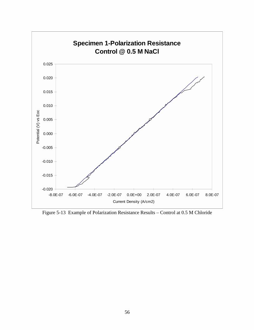
56

Specimen 1-Polarization ResistanceControl @ 0.5 M NaCl

-0.020

-0.015

-0.010

-0.005

0.000

0.005

0.010

0.015

0.020

0.025

-8.0E-07 -6.0E-07 -4.0E-07 -2.0E-07 0.0E+00 2.0E-07 4.0E-07 6.0E-07 8.0E-07

Current Density (A/cm2)

Pote

ntia

l (V)

vs

Eoc

Figure 5-13 Example of Polarization Resistance Results – Control at 0.5 M Chloride

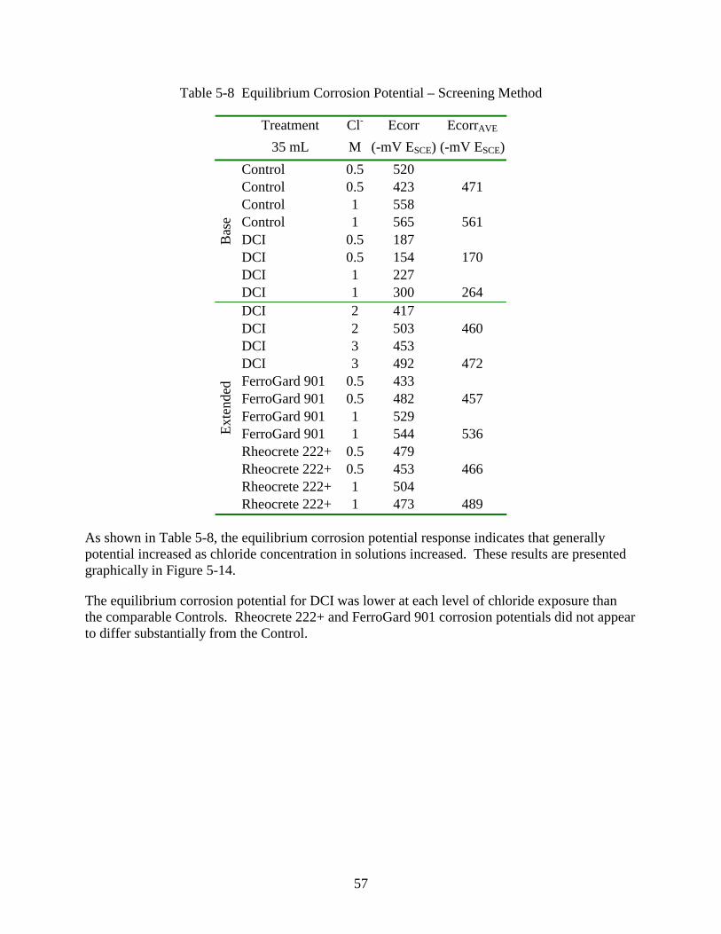
57

Table 5-8 Equilibrium Corrosion Potential – Screening Method

Treatment Cl- Ecorr EcorrAVE

35 mL M (-mV ESCE) (-mV ESCE) Control 0.5 520 Control 0.5 423 471 Control 1 558 Control 1 565 561 DCI 0.5 187 DCI 0.5 154 170 DCI 1 227

Bas

e

DCI 1 300 264 DCI 2 417 DCI 2 503 460 DCI 3 453 DCI 3 492 472 FerroGard 901 0.5 433 FerroGard 901 0.5 482 457 FerroGard 901 1 529 FerroGard 901 1 544 536 Rheocrete 222+ 0.5 479 Rheocrete 222+ 0.5 453 466 Rheocrete 222+ 1 504

Exte

nded

Rheocrete 222+ 1 473 489

As shown in Table 5-8, the equilibrium corrosion potential response indicates that generally potential increased as chloride concentration in solutions increased. These results are presented graphically in Figure 5-14.

The equilibrium corrosion potential for DCI was lower at each level of chloride exposure than the comparable Controls. Rheocrete 222+ and FerroGard 901 corrosion potentials did not appear to differ substantially from the Control.

58

Figure 5-14 Corrosion Potential Response

Corrosion Potential Response

0

100

200

300

400

500

600

0 0.5 1 1.5 2 2.5 3

Chloride Concentration (M Cl-)

Ecor

r (-m

V vs

ER

EF)

Rheocrete 222+Control

Corrosion Potential Response

0

100

200

300

400

500

600

0 0.5 1 1.5 2 2.5 3

Chloride Concentration (M Cl-)

Ecor

r (-m

V vs

ER

EF)

FerroGard 901Control

Corrosion Potential Response

0

100

200

300

400

500

600

0 0.5 1 1.5 2 2.5 3

Chloride Concentration (M Cl-)

Ecor

r (-m

V vs

ER

EF)

DCIControl

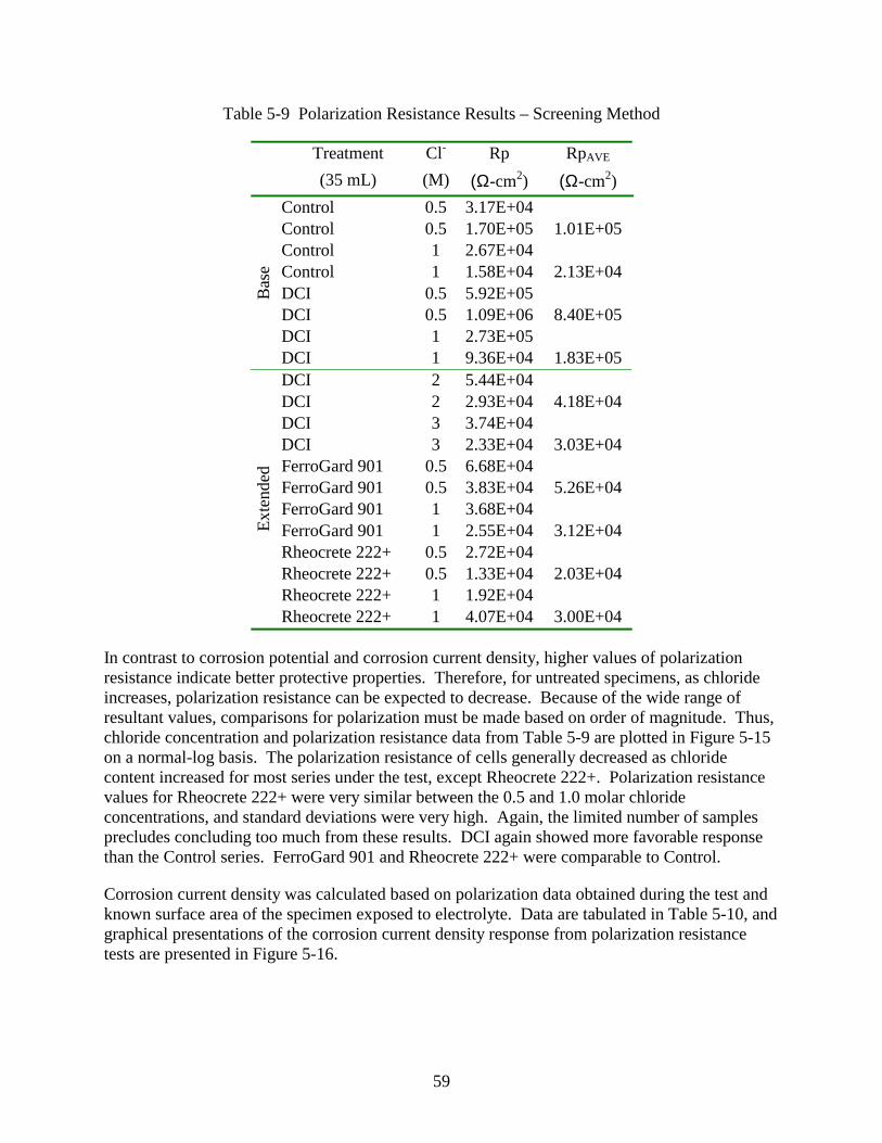
59

Table 5-9 Polarization Resistance Results – Screening Method

Treatment Cl- Rp RpAVE

(35 mL) (M) (Ω-cm2) (Ω-cm2) Control 0.5 3.17E+04 Control 0.5 1.70E+05 1.01E+05 Control 1 2.67E+04 Control 1 1.58E+04 2.13E+04 DCI 0.5 5.92E+05 DCI 0.5 1.09E+06 8.40E+05 DCI 1 2.73E+05

Bas

e

DCI 1 9.36E+04 1.83E+05 DCI 2 5.44E+04 DCI 2 2.93E+04 4.18E+04 DCI 3 3.74E+04 DCI 3 2.33E+04 3.03E+04 FerroGard 901 0.5 6.68E+04 FerroGard 901 0.5 3.83E+04 5.26E+04 FerroGard 901 1 3.68E+04 FerroGard 901 1 2.55E+04 3.12E+04 Rheocrete 222+ 0.5 2.72E+04 Rheocrete 222+ 0.5 1.33E+04 2.03E+04 Rheocrete 222+ 1 1.92E+04

Exte

nded

Rheocrete 222+ 1 4.07E+04 3.00E+04

In contrast to corrosion potential and corrosion current density, higher values of polarization resistance indicate better protective properties. Therefore, for untreated specimens, as chloride increases, polarization resistance can be expected to decrease. Because of the wide range of resultant values, comparisons for polarization must be made based on order of magnitude. Thus, chloride concentration and polarization resistance data from Table 5-9 are plotted in Figure 5-15 on a normal-log basis. The polarization resistance of cells generally decreased as chloride content increased for most series under the test, except Rheocrete 222+. Polarization resistance values for Rheocrete 222+ were very similar between the 0.5 and 1.0 molar chloride concentrations, and standard deviations were very high. Again, the limited number of samples precludes concluding too much from these results. DCI again showed more favorable response than the Control series. FerroGard 901 and Rheocrete 222+ were comparable to Control.

Corrosion current density was calculated based on polarization data obtained during the test and known surface area of the specimen exposed to electrolyte. Data are tabulated in Table 5-10, and graphical presentations of the corrosion current density response from polarization resistance tests are presented in Figure 5-16.

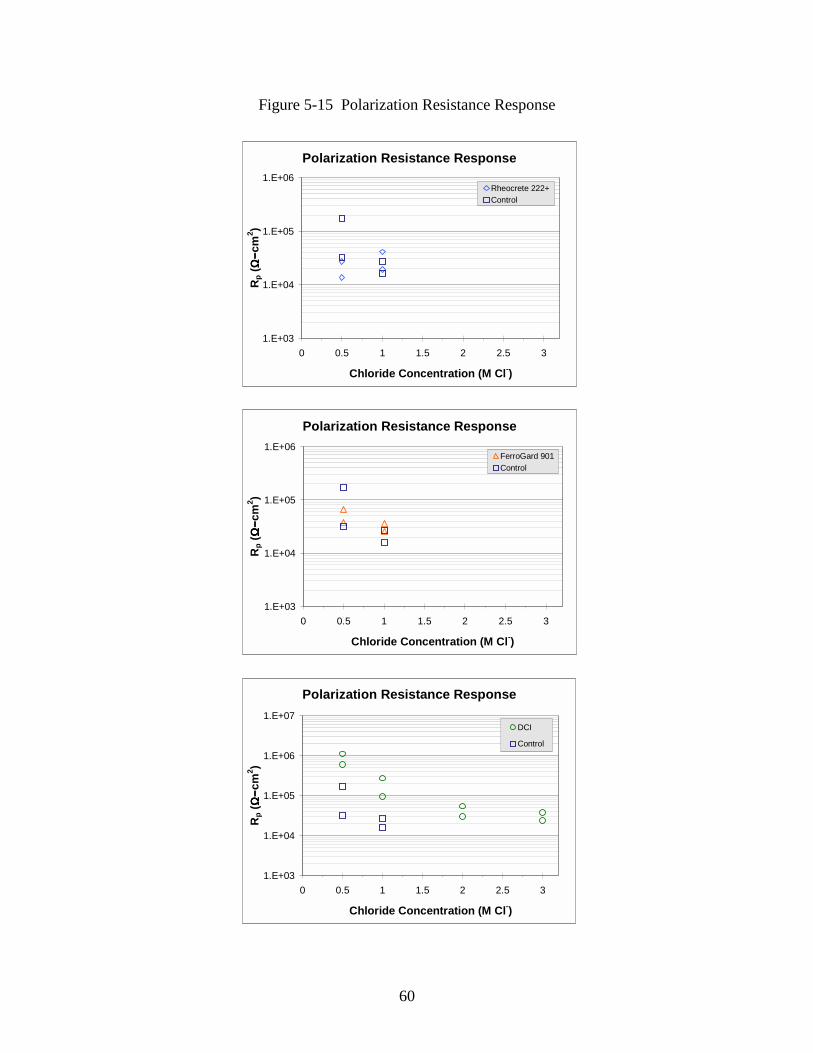
60

Figure 5-15 Polarization Resistance Response

Polarization Resistance Response

1.E+03

1.E+04

1.E+05

1.E+06

0 0.5 1 1.5 2 2.5 3

Chloride Concentration (M Cl-)

Rp (

Ω−

Ω−

Ω−

Ω−c

m2 )

Rheocrete 222+Control

Polarization Resistance Response

1.E+03

1.E+04

1.E+05

1.E+06

0 0.5 1 1.5 2 2.5 3

Chloride Concentration (M Cl-)

Rp (

Ω−

Ω−

Ω−

Ω−c

m2 )

FerroGard 901Control

Polarization Resistance Response

1.E+03

1.E+04

1.E+05

1.E+06

1.E+07

0 0.5 1 1.5 2 2.5 3

Chloride Concentration (M Cl-)

Rp (

Ω−

Ω−

Ω−

Ω−c

m2 )

DCI

Control

61

Table 5-10 Corrosion Current Density – Screening Method

Treatment Cl- Icorr IcorrAVE

(35 mL) (M) (µA/cm2) (µA/cm2) Control 0.5 0.823 Control 0.5 0.153 0.488 Control 1 0.976 Control 1 1.646 1.311 DCI 0.5 0.044 DCI 0.5 0.024 0.034 DCI 1 0.096

Bas

e

DCI 1 0.278 0.187 DCI 2 0.479 DCI 2 0.891 0.685 DCI 3 0.697 DCI 3 1.118 0.908 FerroGard 901 0.5 0.390 FerroGard 901 0.5 0.680 0.535 FerroGard 901 1 0.707 FerroGard 901 1 1.022 0.865 Rheocrete 222+ 0.5 0.957 Rheocrete 222+ 0.5 1.956 1.457 Rheocrete 222+ 1 1.354

Exte

nded

Rheocrete 222+ 1 0.640 0.997

In general, as chloride concentration increased, the associated corrosion current density increased. This was true for the Control, DCI, and FerroGard 901 series. For the Rheocrete 222+ series, the opposite trend was suggested, in which corrosion current density response decreased as chloride concentration increased. However, confidence limits for the data indicated that no statistical difference could be demonstrated. This is due to the fact that only two samples per concentration level were tested in this study. Compiled data from the complete round robin study might provide sufficient sample size to reduce experimental error and differentiate significant response trends. However, that data and analysis are not available at this time and beyond the scope of this study.

Again, corrosion current density appeared to be significantly lower for DCI than Control. Corrosion current density values for FerroGard 901 and Rheocrete 222+ were comparable to Control specimens. Since corrosion current density is derived directly from polarization resistance values and individual Tafel values (βa and βc) for each specimen were not estimated, the relative indications of corrosion performance are identical to those determined by comparing Rp values.

62

Figure 5-16 Corrosion Current Density Response

Corrosion Current Density Response

0.0

0.5

1.0

1.5

2.0

2.5

0 0.5 1 1.5 2 2.5 3

Chloride Concentration (M Cl-)

Icor

r (µ µµµ

A/cm

2 )

Rheocrete 222+

Control

Corrosion Current Density Response

0.0

0.5

1.0

1.5

2.0

2.5

0 0.5 1 1.5 2 2.5 3

Chloride Concentration (M Cl-)

Icor

r (µ µµµ

A/cm

2 )

FerroGard 901

Control

Corrosion Current Density Response

0.0

0.5

1.0

1.5

2.0

2.5

0 0.5 1 1.5 2 2.5 3

Chloride Concentration (M Cl-)

Icor

r (µ µµµ

A/cm

2 )

DCI

Control

63

orelc fff ×=

6 DISCUSSION

The study was designed to assess the relative performance of corrosion inhibiting admixtures under laboratory conditions. Inhibitor performance must be addressed in two stages: 1) effects of inhibitor admixtures on concrete properties, 2) performance of the inhibitors with regard to corrosion reduction in concrete and simulated pore solutions. A secondary objective was to relate the evaluation methods.

Admixture Effects on Concrete Properties

Material Properties of Concrete Cells and Companion Specimens

Performance Criteria

Admixture performance was assessed within concrete specimens, relative to the potential for positive or negative effects on characteristic concrete properties. Such properties include heat of hydration, compressive strength, electrical indication of chloride ion permeability, as well as measured chloride diffusion.

In addition to considering the individual results of the tests outlined above, as related in Chapter 5, comparison and contrast of the tests were made to identify trends or systematic behavioral changes induced by the admixtures. Before discussing the specific relationships for each admixture series, clarification and additional steps of analysis are necessary for certain of the tests presented.

Compressive Strength

Compressive strength results for individual series were discussed in Chapter 5. It was noted for example, that consistently low average compressive strengths for Catexol 1000 and Rheocrete 222+ might be partially the result of increased air content in those specimens, relative to Control concrete.

Popovics presented a numerical relation for the effect of entrained and entrapped air content on concrete compressive strength, based on previous work by others.60 He reported strong correlation with the results of several independent studies by various researchers.

Equation 6-1

where fo = strength of concrete that is air-free in the fresh state

Equation 6-2

where a = air content of the fresh concrete, % γ = 0.0384 for a < 30% and ages 7 to 90 days (suggested by correlated test data)

arelf γ−=10

64

Equation 6-1 and Equation 6-2 together can be used to estimate the compressive strength at an assumed air content, based on the measured compressive strength at a known air content. In this way, the average compressive strengths for each concrete batch were “adjusted” to an equivalent compressive strength at 6.0% air content. Statistical comparison of the adjusted values was conducted to determine differences in 28-day compressive strength between Control and admixture-containing concretes, with air content eliminated as a factor. As with the comparison of direct compressive strength results, the analysis of adjusted strengths revealed significant differences (α=0.05) in 28-day compressive strength for all inhibitors, relative to Control concrete.

Table 6-1 28-day Compressive Strengths Adjusted to 6.0% Air

Admixture Series Average StDev Coeff. Of Var. Relation to Control

Control 6,150 250 4.1% - DCI-S 7,170 330 4.6% 17% Higher Rheocrete 222+ 5,490 320 5.8% 11% Lower FerroGard 901 7,030 170 2.4% 14% Higher MCI-2005 7,260 190 2.6% 18% Higher Catexol 1000 4,850 140 2.9% 21% Lower

Chloride Penetrability by Electrical Conductance

As discussed previously and as the title clearly states, ASTM C 1202 – 94 "Standard Test Method for Electrical Indication of Concrete's Ability to Resist Chloride Ion Penetration" is not an exact measure of permeability, but an indicator.

Table 6-2 Chloride Ion Penetrability Based on Charge Passed26

Charge Passed (coulombs) Chloride Ion Penetrability > 4,000 High

2,000 – 4,000 Moderate 1,000 – 2,000 Low 100 – 1,000 Very Low

< 100 Negligible

According to Table 6-2, excerpted from ASTM C 1202-94, a total charge passed of 4,000 coulombs is the threshold value above which concrete is considered to have “high” chloride ion penetrability. Average chloride penetrability by electrical conductance results for each series at 28 days of age were very close to or exceeded 4,000 coulombs charge passed. However, at 365 days of age, the average charge passed for all series were within the “moderate” range for chloride ion permeability.

Chloride diffusion

The concrete prisms, after cyclic exposure to 6 percent sodium chloride solution, have shown significant variation in the relative diffusion of chloride into the concrete. Acid-soluble chloride

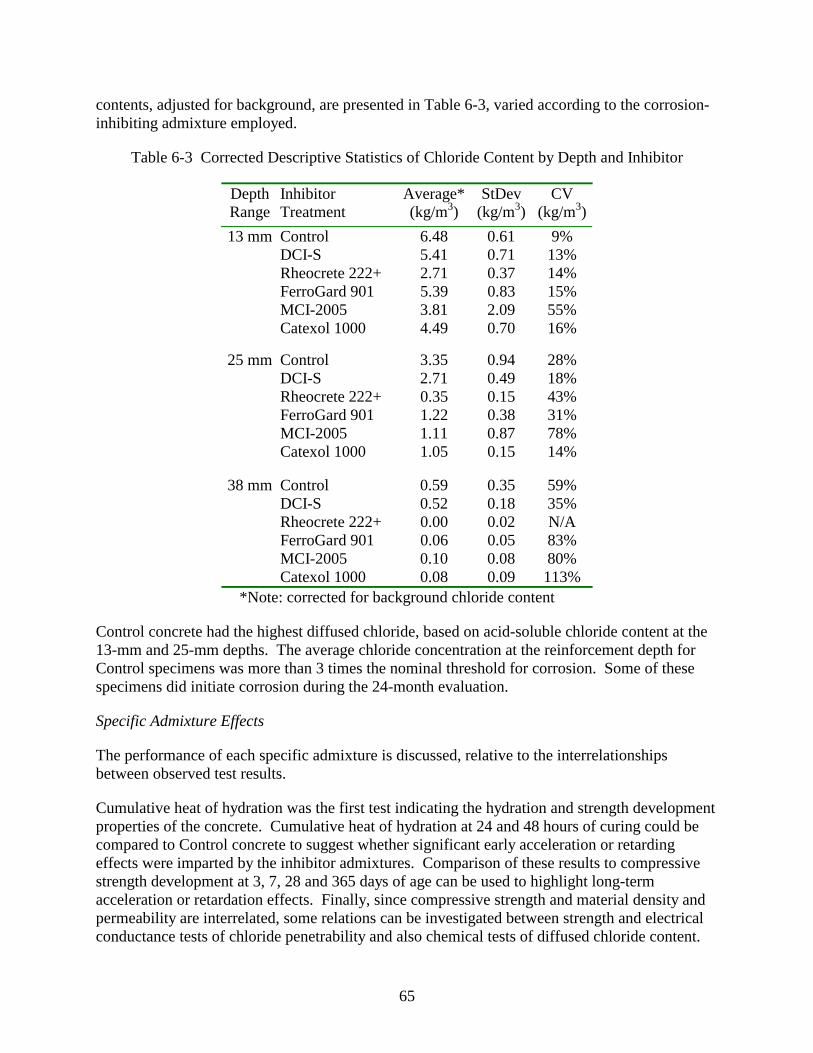
65

contents, adjusted for background, are presented in Table 6-3, varied according to the corrosion-inhibiting admixture employed.

Table 6-3 Corrected Descriptive Statistics of Chloride Content by Depth and Inhibitor

Depth Inhibitor Average* StDev CV Range Treatment (kg/m3) (kg/m3) (kg/m3) 13 mm Control 6.48 0.61 9%

DCI-S 5.41 0.71 13% Rheocrete 222+ 2.71 0.37 14% FerroGard 901 5.39 0.83 15% MCI-2005 3.81 2.09 55% Catexol 1000 4.49 0.70 16%

25 mm Control 3.35 0.94 28% DCI-S 2.71 0.49 18% Rheocrete 222+ 0.35 0.15 43% FerroGard 901 1.22 0.38 31% MCI-2005 1.11 0.87 78% Catexol 1000 1.05 0.15 14%

38 mm Control 0.59 0.35 59% DCI-S 0.52 0.18 35% Rheocrete 222+ 0.00 0.02 N/A FerroGard 901 0.06 0.05 83% MCI-2005 0.10 0.08 80% Catexol 1000 0.08 0.09 113%

*Note: corrected for background chloride content

Control concrete had the highest diffused chloride, based on acid-soluble chloride content at the 13-mm and 25-mm depths. The average chloride concentration at the reinforcement depth for Control specimens was more than 3 times the nominal threshold for corrosion. Some of these specimens did initiate corrosion during the 24-month evaluation.

Specific Admixture Effects

The performance of each specific admixture is discussed, relative to the interrelationships between observed test results.

Cumulative heat of hydration was the first test indicating the hydration and strength development properties of the concrete. Cumulative heat of hydration at 24 and 48 hours of curing could be compared to Control concrete to suggest whether significant early acceleration or retarding effects were imparted by the inhibitor admixtures. Comparison of these results to compressive strength development at 3, 7, 28 and 365 days of age can be used to highlight long-term acceleration or retardation effects. Finally, since compressive strength and material density and permeability are interrelated, some relations can be investigated between strength and electrical conductance tests of chloride penetrability and also chemical tests of diffused chloride content.

66

Control

Control concrete exhibited average compressive strengths near the middle of the range at all ages tested. Cumulative heat of hydration for Control at 24 and 48 hours was near the high end of the range for all series tested. Correspondingly, the peak hydration temperature occurred at the relatively early time of 12 hours after casting. Diffused chloride was highest for Control concrete, even though the total charge passed under the electrical conductance test was near the median of all the groups.

DCI-S

Cumulative heat of hydration at 24 hours after batching showed DCI-S at the high end, slightly above that of the Control group, which is consistent with an accelerated hydration effect. This corresponds to the earliest peak hydration temperature of all the groups, at 10.9 hours after casting. Cumulative heats of hydration for DCI-S after 48 hours were comparable to that of the Control. This suggests that acceleration effects of calcium nitrite were relatively short-lived. This is not inconsistent with compressive strength results for the series. Accelerated early hydration theoretically results in a more porous cement paste structure, and hence lower long-term compressive strength.61 Compressive strengths for DCI-S after 365 days of curing, as compared to Control, were significantly higher than Control.

Diffused chloride content, as corrected for background, was comparable to Control. Chloride penetrability by electrical conductance results show that the total charge passed through specimens containing DCI-S is greater than that of the Control samples at both 28 and 365 days of age. ASTM C 1202-94 specifically warns that the procedure can produce misleading results, as higher coulomb values are generally observed when calcium nitrite, the active ingredient of DCI and DCI-S, is admixed, as compared to controls of the same concrete mixture proportions without calcium nitrite. Our observations appear to support this conclusion.

While chloride penetrability by electrical conductance results for DCI-S were higher than that of Control, the diffused chloride content at reinforcement depth was less or comparable to Control. Thus an early acceleration effect imparted by DCI-S resulted in higher compressive strengths at all ages, and did not cause an increase in permeability or long-term reduction of strength.

Rheocrete 222+

Rheocrete 222+ exhibited 23% less heat evolved from heat of hydration after 24 hours curing. For cumulative heat of hydration through 48 hours of curing, after specimens had returned to laboratory temperature, Rheocrete 222+ specimens had approximately 15% less total heat evolved than the Controls. In addition, peak hydration temperature occurred at 14.1 hours after casting, more than 2 hours later than the Controls. This suggests that Rheocrete 222+ imparts a persistent retarding effect on hydration. Compressive strength results for Rheocrete 222+ were lower than Controls at all ages tested, and serve to emphasize the long-term retarding effect.

Rheocrete 222+, whose manufacturer touts slower ingress of chlorides and moisture as the product's first line of defense, did indeed exhibit a much lower level of diffused chloride than Control mixtures. Comparison of electrical conductance test results for Rheocrete 222+ agree

67

with the diffused chloride results, showing a lower average total charged passed. However, considering the evaluation criteria outlined in Table 6-2, the two series cannot be classified differently at either 28 or 365 days of age under the ASTM C1202-94 test.

FerroGard 901 Cumulative heat of hydration results for FerroGard 901 were 18% and 6% lower than Controls at 24 and 48 hours, respectively. Peak temperature occurred at 13.2 hours, a little over 1 hour later than Controls. These results suggest an early retarding effect that recedes within the first few days of curing. Compressive strength results, even when the effects of the 0.7% lower air content of FerroGard are negated, show an increasing margin of strength gain over the Control concrete with time. For FerroGard 901, electrical conductance for chloride penetrability values and diffused chloride contents were both less than Control. The total charge passed for FerroGard 901 at 28 days age was less than 4,000 coulombs, placing that material in the moderate range for permeability, while control at that age was considered highly permeable. At 365 days of age, ASTM 1202-94 results for FerroGard 901 and Control were comparable, and both would be considered moderately permeable to chloride ion. Diffused chloride in FerroGard 901 specimens after two years was significantly lower than Control. Therefore, early retarding effects were evident, but did not extend beyond the earliest phases of curing.

MCI-2005

Near the low end of 24-hour heat of hydration results was MCI-2005. Peak hydration temperature occurred at a very late 15.5 hours after casting. By contrast, the cumulative heat of hydration for MCI-2005 approached that of the Control series after 48 hours curing. Therefore, early retarding effects suggested by the 24-hour results do not seem to translate to the long-term for MCI-2005. Compressive strength values for MCI-2005 were comparable to Control concrete at very early ages, but outperformed Controls in long-term compressive strength development.

Concrete containing MCI-2005 had significantly less diffused chloride at reinforcement depth, and electrical conductance values were very similar to Control. According to Table 6-2, concrete containing MCI-2005 in this study would also be classified as moderately permeable. The MCI –2005 admixture produced significant benefits in reduction of concrete permeability and long-term strength development, as indicated by strength results and diffused chloride measurements.

Catexol 1000 Cumulative heat of hydration for Catexol 1000 was 9% and 5% lower than Control at 24 and 48 hours of curing, respectively. The peak hydration temperature occurred 2.2 hours later than Control. Compressive strength results showed a large reduction in compressive strength for Catexol 1000 at all ages, even when the effects of a 0.9% increase in air content are taken into

68

consideration. Compressive strengths, adjusted for air content, at 28-days of age indicate a reduction of 21% in compressive strength between Catexol 1000 and Control. An important detail is that, due to a shortage of material, the third specimen of the MCI-2005 series and all of the Catexol 1000 series concrete used a Type I/II cement, rather than the Type I cement used in all other specimens. Chemical analyses of the cements are presented in Appendix A - Concrete And Reinforcement Material Parameters. Cumulative heat of hydration for MCI-2005 Specimen 3 was noticeably less than that of Specimens 1 & 2. However, compressive strength data for MCI-2005 Specimen 3, as compared to Specimens 1 & 2, shows comparable strength gain at all ages. Therefore, it does not appear that the alternate cement is responsible for the lack of strength development in the Catexol 1000 specimens. Catexol 1000 had significantly less diffused chloride at reinforcement depth, but electrical conductance values were significantly higher than Control. The higher conductance values and lower compressive strengths seem to be complimentary, but are contradicted by reduction of diffused chloride. Heat of hydration data, coupled with compressive strength development does not seem to suggest an early set-retarding reaction, but an overall reduction in hydration over the life of the concrete, as a result of the Catexol 1000 admixture. Positive benefits with regard to chloride diffusion are inferred.

Summary of Concrete Properties Evaluation

Strength and Hydration Effects

Comparison of time of peak temperature to compressive strength gain suggests a correlation. Those admixtures which tended to delay the peak temperature at initial hydration also showed lower average strength gain at all ages, with the disparity in compressive strength increasing over time.

Heat of hydration, coupled with compressive strength and electrical indication of chloride permeability can highlight underlying effects on rate and degree of hydration caused by the inhibitors.

Chloride Diffusion and Chloride Penetrability by Electrical Conductance

The relation was investigated between chloride penetrability by electrical conductance results after 28-days and 1 year of curing and diffused chloride at reinforcement depth after two years of ponding. Measurements of electrical indication of chloride penetrability should not be taken independently, but correlated with diffused chloride measurements.

Each of the inhibitors appeared to slow the ingress of chloride into the concrete over the 24-month evaluation period, except DCI-S, which was comparable to Control. Chloride concentration is highly variable, as demonstrated in the tables. High concentration at a single point of sampling may not necessarily indicate uniformly high concentrations at the steel surface. Alternatively, chloride concentration at steel depth may not be uniform, and localized areas of

69

high chloride concentration are possible along the steel surface, which may lead to localized or pitting corrosion.

Inhibitor Performance

Electrochemical Measurements in Concrete Cells

Performance Criteria

Electrochemical corrosion performance was monitored monthly via three tests: macro cell corrosion current measurements, electrical half-cell potential measurements and corrosion current density using the three-electrode linear polarization technique. Where applicable, visual assessment of time-to-cracking of concrete cover was used to confirm significant corrosion activity.

As outlined in Table 2-1, and electrical potential more negative than –350 millivolts CSE indicates a high probability of corrosion. Macro-cell corrosion current, as detailed in ASTM G109-92, indicates active corrosion when measured current exceeds 10 µA. Clear has suggested the following interpretation for corrosion current density results obtained using the 3LP device and software:59

Table 6-4 Interpretation Guidelines for Corrosion Current Density

Icorr (mA/sf) Icorr (µA/cm2) Prognosis < 0.20 < 0.22 No corrosion damage expected

0.20 to 1.0 0.22 to 1.1 Corrosion damage possible in the range of 10 to 15 years 1.0 to 10 1.1 to 11 Corrosion damage expected in 2 to 10 years

> 10 > 11 Corrosion damage expected in 2 years or less

Liu demonstrated that the measured corrosion rate from linear polarization devices, such as the 3LP, only represent instantaneous values, and must be adjusted for prevailing environmental conditions and correlated with long-term weight loss measurements.15 In general, he observed that the 3LP method tends to overestimate the average corrosion rate.

Control

Chloride content at reinforcement depth far exceeded the nominal threshold for corrosion in untreated reinforced concrete. Active corrosion has been measured by the electrochemical methods in one bar triad of each of Control specimens 1 & 2. Both triads in Control Specimen 3 have undergone extensive corrosion, and cover concrete has cracked.

Control specimen 3 showed elevation of electrical potential and macro-cell corrosion current after only 3 months of ponding. Cracking of the cover concrete over the top bar in cell "b" occurred 6 months after corrosion initiation was indicated. The second cell of this specimen initiated corrosion at approximately the same time, but cracking of the cover concrete was not observed until approximately 9 months after initiation.

70

Visual inspection of the specimen has not revealed any indication of the cause of premature corrosion activity. One potential explanation for the corrosion activity in Control Specimen 3 is crevice corrosion. Despite efforts to the contrary, this might have occurred along the bar at the end of the electroplating tape and neoprene tubing. This can be verified only by a destructive autopsy of the specimen at the completion of the evaluation.

DCI-S

Chloride at the reinforcement depth of DCI-S concrete specimens significantly exceeds the nominal threshold for corrosion. No indications of active corrosion have been detected by electrochemical methods. The admixture appears to be effectively inhibiting the corrosion reaction.

Rheocrete 222+

Chloride at the steel depth within Rheocrete 222+ specimens has not yet reached the nominal threshold for corrosion. Corrosion has not been indicated by electrochemical tests. Since sufficient chloride has not diffused, no conclusion can be reached as to the corrosion inhibiting performance of Rheocrete 222+ at this time.

It is interesting to note that the Rheocrete 222+ series exhibited half cell potential values significantly lower than the other treatment samples and that the potentials continued a downward trend over time, approaching a reference potential of approximately 0 millivolts relative to the copper sulfate electrode. However, these specimens were the only ones that had not yet reached threshold chloride levels.

FerroGard 901

Chloride concentrations at the reinforcing steel depth are above the nominal threshold for corrosion. Corrosion activity has not been detected by electrochemical techniques. Some corrosion inhibiting benefit appears to have been gained, but further monitoring is warranted.

MCI-2005

Chloride concentrations at steel depth are slightly above the nominal threshold for corrosion. Corrosion activity has not been indicated by electrochemical tests. Thus far, benefit with regard to corrosion inhibition is apparent, but requires further observation.

Catexol 1000

Chloride at steel depth just barely exceeds the nominal threshold for corrosion. No evidence of corrosion has been observed under the electrochemical tests. Further monitoring is needed.

Summary of Concrete Cell Tests

None of the specimens, other than Controls, have exhibited any electrochemical indications of corrosion activity or related cracking during the 24-month evaluation.

71

Using data from the Control cells, which did exhibit active corrosion, excellent correlation was made between measured initiation of macro-cell corrosion, and an associated increase in electrical potential, as well as increasing corrosion current density as measured by the 3LP device. An increase in amplitude under each test occurred at approximately the same time, when significant corrosion activity began. However, macro-cell current electric potential readings showed rather severe spikes in observed corrosion activity when compared to the linear polarization response, which tended to increase gradually over time. The macro-cell corrosion activity between reinforcement layers, as measured by the former, is only part of that corrosion activity measured by the 3LP, since linear polarization indicates a mixed-cell response. Therefore, the gradual increase likely reflects the development of localized corrosion cells on the top reinforcement bar over time.

Macro-cell measurements provide peak corrosion current for the cell. By contrast, the linear polarization response is averaged over the polarized surface of the bar, presuming uniform corrosion. This assumption will tend to “dilute” the results, as compared to the macro-cell current technique. However, if macro-cell current is converted to current density, by also considering corrosion to be spread over the exposed bar area, macro-cell measurements will tend to underestimate absolute corrosion, as localized (micro-cell) corrosion is not measured. Berke has stated that the macro-cell current method is suitable for comparing inhibitors in similar specimens, but should not be interpreted as an indication of absolute corrosion rates.47

As stated previously only the Control series contained cells with significant macro-cell corrosion current within the 24 month evaluation. No measurable macro-cell corrosion current was identified in any of the inhibitor treatment samples. The same case was true with regard to linear polarization response. Measured corrosion current density for each of the inhibited series remained at a nominal level, generally below 0.50 micro-amps per square centimeter.

Therefore, the observed corrosion current density for each cell indicate that, other than the Control specimens already mentioned, no substantial corrosion related damage could be predicted in the short-term for the specimens, based on 3LP testing through the end of the 24-month evaluation. Half-cell electrical potential values remained in the range generally considered to indicate low or uncertain probability of corrosion.

With the exception of concrete containing Rheocrete 222+, all of the specimens exhibited chloride concentrations at the depth of the reinforcing steel in excess of the conventional threshold for corrosion. A conservative figure is 0.9 kilograms of diffused (measured minus background) chloride per cubic meter of concrete.9,12 Given consideration to these conditions, it appears that all the CIA’s are presently providing some level of corrosion protection.

Simulated Pore Solution Immersion Tests

Performance Criteria

The purpose of the simulated pore solution immersion test was to provide an accelerated test method which would specifically address the corrosion inhibiting performance of admixtures in a high-pH environment similar to concrete, without the influence of the diffusion process and

72

concrete characteristics. The method was designed to gage the potential for a given inhibitor to reduce overall corrosion of steel directly exposed to aggressive chloride ions in solution.

Some information was sought regarding the dependency of inhibitor effectiveness on inhibitor and chloride concentrations. Previous research by others has established that performance of many anodic inhibitors is directly dependent on the mass ratio of active inhibiting ingredient to chloride present in solution. The simulated pore solutions included select dosages of inhibitor and concentrations of chloride ion, in an attempt to distinguish the limiting ratios of chloride to inhibitor for each admixture.

Both relative weight loss and corroded surface area results are presented in Chapter 5. Following is an analysis and discussion of the findings, as well as a comparison between the two sets of measurements. As a general comment regarding the interpretation of weight loss and surface area corrosion results, in the case of uniform corrosion, weight loss should be considered as the primary indicator of corrosion performance. Surface area corrosion could be used in gaging tendency toward uniform versus pitting corrosion. ASTM G 1-90 clearly indicates "… mass losses can be misleading when deterioration is highly localized, as in pitting or crevice corrosion."46 However, weight loss, when supplemented by surface area corrosion data may more clearly indicate propensity for pitting corrosion.

Figure 6-1 Relation of Weight Loss to Corroded Surface Area

After direct comparison of weight loss and corroded surface area for each series, an attempt was made to find a correlation between the two measurements. Figure 6-1 presents a conceptual model for interpreting weight loss and corroded surface area where pitting is potentially occurring.

73

When plotted, a linear trend could be observed for the Control specimens in which relative surface area corroded increased as relative weight loss increased. The trend can be observed when relative percent weight loss is plotted directly against relative surface area corroded, as illustrated in Figure 6-2.

ControlWeight Loss vs Corroded Surface Area

Relation within Treatment Series

-50.0%

-40.0%

-30.0%

-20.0%

-10.0%

0.0%

10.0%

20.0%

30.0%

40.0%

50.0%

-0.20% -0.15% -0.10% -0.05% 0.00% 0.05% 0.10% 0.15% 0.20%

Relative Weight Loss (%)

Rel

ativ

e Su

rfac

e A

rea

Cor

rode

d (%

)

Control

NOTE: Values are relative to Control with no chloride (control)

Figure 6-2 Weight Loss versus Corroded Surface Area – Control

The points in the graph are connected by lines which proceed consecutively in order of increasing chloride exposure, starting at point (0,0) for the no-chloride group, which is the benchmark for measurement. Recall that the subsequent chloride concentrations are 0.2, 0.28, 0.6, 0.77, 1.17, and 1.61 molar chloride, respectively. For the Control series, the resulting correlation falls neatly in quadrant I, where weight loss and surface area directly correspond, and uniform corrosion is prevalent.

Rheocrete 222+

Rheocrete 222+ was used in solution at a single dosage rate equivalent to 5 liters of inhibitor per cubic meter of concrete, as recommended by the manufacturer. Rheocrete 222+ showed an increase in surface area corrosion relative to steel in untreated solutions at lower and intermediate levels of chloride exposure. Average percentages of corroded surface area were higher at more extreme chloride concentrations, but the differences were not statistically significant.

Results of Rheocrete 222+ performance with regard to relative weight loss were mixed. Inhibiting effects, as reflected by relative weight loss results, are shown at the middle and high extremes of chloride exposure under the test. Yet at low chloride exposure and at a level between the moderate and high exposures, behavior is no different than that of Control

74

specimens. On the basis of relative weight loss, Rheocrete 222+ was benign at worst and, at best, provided significant inhibiting effects at intermediate levels of chloride exposure.

Rheocrete 222+Weight Loss vs Corroded Surface Area

Relation within Treatment Series

-50.0%

-40.0%

-30.0%

-20.0%

-10.0%

0.0%

10.0%

20.0%

30.0%

40.0%

50.0%

-0.20% -0.15% -0.10% -0.05% 0.00% 0.05% 0.10% 0.15% 0.20%

Relative Weight Loss (%)

Rel

ativ

e Su

rfac

e A

rea

Cor

rode

d (%

)

Rheocrete 222+ (5L/m3)

NOTE: Values are relative to Rheocrete 222+ at 5 L/m3 dosage and no chloride (control)

Figure 6-3 Weight Loss versus Corroded Surface Area – Rheocrete 222+

No linear relation between weight loss and corroded surface area could be found for Rheocrete 222+, as shown in Figure 6-3. When comparing surface area results to those of the weight loss experiment, one might conclude that Rheocrete 222+, at intermediate levels of chloride exposure, effectively reduced overall loss of base metal due to corrosion, and the type of corrosion shifted away from pitting, toward a more uniform surface corrosion. This behavior, if reproduced within the concrete matrix, can be beneficial in reducing the severity of localized damage due to insidious pitting corrosion, but is classified as corrosion nonetheless.

In general, Rheocrete 222+ cannot be found to have effectively prevented corrosion of bar specimens immersed in simulated pore solution.

FerroGard 901

Samples in solutions containing FerroGard 901 at two dosages, equivalent to 10 and 15 liters of inhibitor per cubic meter of concrete, also exhibited mixed performance results with regard to relative surface area corroded and relative weight loss.

FerroGard 901 at 10 liters per cubic meter

Observation of surface area corrosion results for FerroGard 901 at 10 liters per cubic meter concentration reveal an increase in relative surface area corroded at lower exposures in a range of 0.20 and 0.28 molar chloride. A slight reduction in average surface area corroded relative to

75

Control could be observed at a moderate exposure range of 0.60 and 0.77 molar chloride, but comparison of statistical results reveals that the differences are not statistically significant. Relative surface area corrosion for FerroGard 901 at 10 liters per cubic meter dosage averaged higher than that of Control in a range from 1.17 to 1.61 molar chloride, with a statistically significant difference at 1.17 molar chloride.

Comparison of weight loss between FerroGard 901 and Control at the 10 liter per cubic meter dosage rate indicated a reduction in weight loss at lower chloride concentrations, an increase at intermediate chloride concentrations, and a reduction at higher concentrations of chloride. This response was almost the inverse of the surface area corrosion results. This relation may reflect a decrease in the tendency to pitting corrosion and some inhibition benefit within certain ranges of chloride concentration. However, it appears that the ability of FerroGard 901 to inhibit corrosion is particularly sensitive to the relative level of chloride present in solution. An unusual aspect of this behavior is that inhibition was observed at low and high concentrations of chloride, with negative effects observed in the middle range of chloride concentration.

FerroGard 901 at 15 liters per cubic meter

Observations of FerroGard 901 performance at the 15 liters per cubic meter dosage rate were also mixed. With regard to relative surface area corroded, FerroGard 901 at this dosage rate averaged higher, but were not significantly different than that of the Control, except at a concentration of 1.61 molar chloride, where a significant reduction in surface area corroded was observed. With regard to relative weight loss, FerroGard 901 at the 15 liters per cubic meter dosage rate exhibited an increase in weight loss relative to the Control specimens at moderate concentrations of 0.6 and 0.77 molar chloride. At lower and higher chloride concentrations, no significant difference from Control was observed. Therefore no inhibiting benefit can be identified from FerroGard 901 at a dosage rate of 15 liters per cubic meter under this test.

76

FerroGard 901Weight Loss vs Corroded Surface Area

Relation within Treatment Series

-50.0%

-40.0%

-30.0%

-20.0%

-10.0%

0.0%

10.0%

20.0%

30.0%

40.0%

50.0%

-0.20% -0.15% -0.10% -0.05% 0.00% 0.05% 0.10% 0.15% 0.20%

Relative Weight Loss (%)

Rel

ativ

e Su

rfac

e A

rea

Cor

rode

d (%

)

FerroGard 901 (10 L/m3)FerroGard 901 (15 L/m3)

NOTE: FerroGard 901 15 L/m3 values are relative to group with FerroGard 901 10 L/m3 dosage and no

chloride (control)

Figure 6-4 Weight Loss versus Corroded Surface Area – FerroGard 901

No linear relation between weight loss and corroded surface area could be found for FerroGard 901, as shown in Figure 6-4. For FerroGard 901 at 15 liters per cubic meter dosage, the significant reduction in surface area corroded at 1.61 molar chloride, in contrast to no relative difference in weight loss, suggests a higher probability of pitting at this level of chloride exposure. Indeed, visual observation of the specimens at high chloride concentration confirms that corrosion activity was concentrated in a few areas, with considerable corrosion product within a short radius. In contrast, specimens under intermediate chloride exposures developed wider-spread, less intense corrosion sites.

DCI

DCI was evaluated at two dosage rates, 10 and 15 liters of inhibitor and per cubic meter of concrete. As discussed earlier, interpretation of the results of testing vary depending on whether comparison is made "between" series or "within" a series. Based on observed differences in Control groups containing no chloride between the two phases of the experiment, comparison "within" a series was deemed appropriate.

DCI at 10 liters per cubic meter

Surface area corrosion for DCI at 10 liters per cubic meter averaged below that of the Controls at all chloride concentration levels. Relative weight loss of DCI at 10 liters per cubic meter dosage was lower than that of the Controls at 0.28 molar chloride, not statistically different at 0.6 molar chloride, and higher than Controls at 0.77 and 1.17 molar chloride.

77

It would appear that DCI has an inhibiting effect, as reflected in relative weight loss results, up to a concentration level of approximately 0.65 molar chloride. Beyond 0.77 molar chloride concentration, DCI at 10 liters per cubic meter dosage does not have a significant inhibiting effect, and results may indicate greater weight loss than that of the Control. A corresponding significant reduction in corroded surface area may indicate a tendency toward pitting as chloride concentrations overwhelm the nitrite's ability to inhibit. Visual observations confirm that corrosion activity was concentrated in fewer locations, but with greater accumulated corrosion product as chloride concentrations increased.

DCI 15 liters per cubic meter

For DCI at 15 liters per cubic meter dosage, surface area corroded is less than that of the controls at 0.6 and 0.77 molar chloride, but not statistically different (α=0.05) at 1.17 and 1.61 molar chloride. Relative weight loss was significantly less than that of the Controls at concentrations of 0.60 and 0.77 molar chloride, but not statistically different at concentrations of 1.17 and 1.61 molar chloride.

DCI at the higher dosage level of 15 liters per cubic meter appears to provide effective inhibition up to concentrations in excess of 0.77 molar chloride, but did not perform differently from the Controls at chloride concentrations of 1.17 molar and beyond. These results are reflected in both weight loss and corroded surface area measurements.

DCIWeight Loss vs Corroded Surface Area

Relation within Treatment Series

-50.0%

-40.0%

-30.0%

-20.0%

-10.0%

0.0%

10.0%

20.0%

30.0%

40.0%

50.0%

-0.20% -0.15% -0.10% -0.05% 0.00% 0.05% 0.10% 0.15% 0.20%

Relative Weight Loss (%)

Rel

ativ

e Su

rfac

e A

rea

Cor

rode

d (%

)

DCI (10 L/m3) DCI (15 L/m3)

NOTE: DCI 15 L/m3 values are relative to DCI 10 L/m3 dosage and no chloride (control)

Figure 6-5 Weight Loss versus Corroded Surface Area – DCI

A linear relation can be discerned for DCI treated specimens in which increased weight loss is accompanied by slight increase in surface area corroded. Figure 6-5 illustrates this relation. In considering the relation between surface area corrosion and relative weight loss for DCI,

78

observed reductions in surface area corroded directly correspond to the reduction in weight loss due to corrosion, except at extreme chloride exposures, as mentioned previously. This result is consistent with previous reports, which indicate a tendency toward pitting at extreme chloride chloride-to-nitrite ratios.36 Visual observations again confirm this trend.

Summary of Simulated Pore Solution Immersion Tests

Electrochemical Screening Tests

Performance Criteria

The electrochemical screening method was primarily based on the polarization resistance test. From polarization resistance tests, comparison was made between corrosion potential (Figure 5-14), corrosion current density (Figure 5-16), and polarization resistance (Figure 5-15) for each inhibitor at two or more chloride concentrations.

Rheocrete 222+

Corrosion potential for Rheocrete 222+ was plotted against that of the control specimens at 0.5 and 1.0 molar chloride concentration. At 0.5 molar chloride, corrosion potential of the specimen immersed in Rheocrete 222+solution was almost identical to the Control samples. Corrosion potential for Rheocrete 222+ was significantly less than that of the Control at 1.0 molar chloride exposure. Corrosion current density of Rheocrete 222+ was higher than that of Control at 0.5 molar chloride but lower than Control at 1.0 molar chloride. However, 95 percent confidence limits did overlap, indicating no statistical difference between either set of measurements. Comparisons of polarization resistance results correspond. Rheocrete provided a lower polarization resistance than Control at 0.5 molar chloride but a higher polarization resistance at 1.0 molar concentration. Again, no statistical difference can be proven based on these tests.

Polarization resistance results indicate a slight tendency toward inhibition at 1.0 molar chloride based on these three response criteria. The reduction in corrosion potential at 1.0 molar chloride concentration is not directly reflected in corrosion current density and polarization resistance values. However, having only tested two specimens of each treatment, no solid conclusions can be drawn basis of statistical analysis. Therefore, as a screening test, it would be necessary to conduct a larger number of experiments before any determination can be made with regard to potential inhibition response.

FerroGard 901

Corrosion potential of specimens in FerroGard 901 solution were very similar to that of the control group and both 0.5 and 1.0 molar chloride concentration, with a slight statistical reduction shown at 1.0 molar. Corrosion current density for FerroGard 901 was nearly identical to that of the Control group at 0.5 molar chloride exposure and averaged less than Control at 1.0 molar. Limited number of samples resulted in wide variance for each treatment and therefore no statistical difference could be determined. Polarization resistance values were similar at 0.5 chloride concentration, with FerroGard 901 averaging slightly lower than Control. At 1.0 molar chloride concentration, FerroGard 901 showed a beneficially higher average polarization resistance, although the difference was not statistically significant. As with Rheocrete 222+,

79

additional repeat units of each treatment to be required before significant conclusions can be drawn regarding potential inhibiting activity.

DCI

Corrosion potential results for DCI a 0.5 and 1.0 molar chloride concentration were significantly lower than that of the Controls and additional tests at 2.0 and 3.0 molar chloride concentration demonstrated a gradual increase in corrosion potential as chloride concentration increased. At 3.0 molar chloride the corrosion potential of DCI-treated specimens approached that of Control specimens at 0.5 molar chloride. The observed trend suggests DCI does indeed increase the threshold concentration of chloride necessary to raise corrosion potential to levels capable of inducing corrosion.

Corrosion current density of specimens in DCI solution averaged far lower than those of the Control specimens at 0.5 and 1.0 molar chloride concentration, and generally showed a linear trend with increasing chloride exposure. No statistical significance can be on a 0.5 molar chloride concentration, solely due to the fact that the Control specimens exhibited a wide variation between only two specimens. However, at 1.0 molar chloride concentration the reduction in corrosion current density caused by the presence of DCI is clearly significant.

Analysis of polarization resistance measurements shows that DCI on average returned a higher polarization resistance than that of the Controls, with a statistically significant difference at 0.5 molar chloride concentration. Once again, additional tests would be necessary at a 1.0 molar chloride concentration to discern a statistical difference. The plot clearly shows that difference between the average polarization resistance of DCI and Control is almost a full order of magnitude.

Considering the observed response in corrosion potential, corrosion current density, and polarization resistance, it is reasonable to conclude that DCI did exhibit an inhibiting effect relative to Control solutions.

Summary of Screening Tests

Summary and Comparison of Procedures

The researchers wished to find a correlation between the various procedures employed. The first group of procedures involved evaluation of corrosion inhibiting admixtures in a conventional reinforced concrete slab specimen. This method, although well established as an ASTM procedure, can be expensive and time-consuming, as it requires an extended exposure period before results can be obtained.

The second procedure, involving simulated pore solution, eliminates many restrictions common to the conventional concrete slab specimens. The concrete medium was replaced by a solution designed to emulate the pore solution within the concrete system. This eliminates requirements for concrete mixing, casting and curing, eliminates the diffusion element of the deterioration process, and removes relative saturation and the electrical resistance of the concrete material as a variable in the electrochemical system. Thus, the interaction between the reinforcing steel specimen, the contaminant and the pore solution environment containing inhibiting admixtures

80

can be more directly observed. The experimental procedure requires significantly less time, dependent primarily on the desired exposure period, which was approximately 4.5 months for our study.

The third procedure, involving the electrochemical analysis of a standard specimen in a standard corrosion cell after short-term exposure, attempted to provide accelerated testing to screen potential inhibitors for more detailed evaluation. By comparison, this procedure was extremely fast, requiring approximately 2.5 days per specimen to complete.

Relation of Immersion Tests to Concrete Corrosion Cells

The potential for correlation between immersion tests and concrete corrosion cells is limited by the fact that most of the concrete specimens have yet to reach a state of active corrosion. The importance of the pore solution tests is primarily as a yes/no determination of the ability of an admixture to inhibit corrosion under controlled conditions in solution. Such solutions can not possibly be representative of the complex environment around reinforcing steel within concrete. However, by employing a solution screening method, the time and effort required for long-term concrete specimens can be reserved for those substances that demonstrate the greatest promise of success.

The pore solution immersion test is, at best, still only a screening method, and the true performance of any potential corrosion inhibiting admixture for concrete still must rely on benchmark tests involving steel embedded in concrete, such as ASTM G 109-92.

Relation of Screening Tests to Immersion Tests

General Observations

In the electrochemical screening method, as with the simulated pore solution immersion procedure, the concrete medium was replaced by a solution designed to emulate the pore solution of the concrete. Instead of a synthetically designed pore solution, the electrolyte was comprised of filtered cement slurry containing the desired admixtures. Test specimens were a standard size and material source, eliminating physical and metallurgical variations of specimens as a significant factor in the evaluation. One negative feature of the screening method is that it is equipment intensive. A relatively high initial cost is related to acquisition of the computer-based potentiostat system, software, electrochemical cell apparatus, and test specimens.

A potential shortcoming of the procedure, as performed, includes the need for more repeat units at each treatment level, as discussed previously. Another potential concern regards the greatest benefit of this test: the short time frame in which it is performed. It is possible that the pretreatment period is not long enough to allow sufficient time for inhibitors to take effect. Although the test is specifically targeted as a method of screening, results may be biased, particularly against those inhibitors that function by passivation. On the other hand, careful consideration will have to be made as to whether 24 hours is a sufficiently long period of chloride exposure to accurately indicate corrosion performance. Some experience in this regard can be borrowed from previous experience by researchers of pipeline and pressure vessel corrosion.

81

The polarization resistance test employed in the screening method is also particularly sensitive to selection of settings, such as IR compensation, which can affect the outcome of experiments. More specific knowledge of electrochemical theory and techniques is required to properly perform this method than is necessary with the other methods discussed.

By contrast, the simulated pore solution method is simple in design, not particularly equipment intensive, and does not require specialized training to perform. However, the method is much more time consuming, in terms of both exposure times and personnel time involved in the cleaning, weighing, visual assessment and compilation of results.

Problems Precluding Specific Comparison of Results

The dosage of 35 milliliters inhibitor per liter of solution is dictated by the proposed test procedure, and does not specifically account for specific manufacturer's recommended dosage rates for a potential inhibitor. Therefore, is not clear that the dosage rate employed is optimal for some inhibitors.

The response of Rheocrete 222+ under Simulated Pore Solution testing indicated some benefit with regard to weight loss at lower chloride concentrations. The results of the screening test do not provide evidence of any inhibiting benefit at the exposure levels employed. However, the dosage rate for the screening test was fixed at 35 milliliters inhibitor per liter of solution. The dosage rates employed for the simulated pore solution test varied in accordance with manufacturers’ dosage recommendations for concrete. Effectively, the Rheocrete 222+ series contained the equivalent of almost 70 milliliters per liter of solution, twice that of the screening test. The discrepancy arises from the assumed proportion that pore solution comprises in concrete. If pore volume is assumed to be 3 percent of concrete, as derived from Stark, then 70 milliliters of inhibitor solution per liter would be equivalent to 5 liters per cubic meter of concrete.52 However, if 6 percent by volume of concrete is considered pore solution, then 35 milliliters inhibitor per liter of solution, as used in the screening test, would be equivalent to 5 liters inhibitor per cubic meter of concrete. In any case, the differing dosage rates preclude direct comparison of the results. The results of this study show both methods provide some indication of inhibitor efficiency.

82

7 CONCLUSIONS

Evaluation of commercially available corrosion inhibiting admixtures for reinforced concrete was undertaken. The inhibitors were compared by three different evaluation methods, and the results presented herein.

Effects on Concrete Properties

DCI-S

Chloride permeability as indicated by electrical conductance gave higher total charge passed, but this is a previously documented phenomenon, and the test is considered unreliable for this admixture. This is supported by evidence of no statistical difference in diffused chloride for DCI-S. Early accelerated hydration effects were observed, but were not detrimental to handling or performance. DCI-S exhibited an overall positive influence on concrete compressive strength at all ages, and exhibited permeability and diffusion characteristics similar to untreated concrete.

Rheocrete 222+

Rheocrete exhibited a much lower permeability and diffusion of chloride than untreated concrete. A persistent reduction in hydration rate, and subsequently compressive strength, was observed as a result of the Rheocrete 222+ admixture. Therefore, a slightly negative impact on compressive strength must be compensated if this admixture is used.

FerroGard 901

FerroGard 901 had a beneficial effect on permeability and reduced diffusion of chloride. Significant increase in overall compressive strength was another benefit. No particular adverse effects were observed.

MCI-2005

MCI-2005 slightly reduced permeability and lessened the diffusion of chloride into concrete over the test period. Compressive strength was increased over untreated concrete when MCI-2005 was admixed. No adverse effects were observed with regard to handling, setting or curing.

Catexol 1000

Chloride ingress was slightly reduced in concrete containing Catexol 1000. However, chloride penetrability tests by electrical conductance indicated slightly more permeable concrete. Generally, permeability could be classified the same as untreated concrete. Significant reduction in compressive strength at all ages is a primary adverse effect observed. Difficulty in limiting entrained air in the presence of the inhibiting admixture was a factor. The degree of strength loss resulting from the admixture makes it undesirable for applications where compressive strength is the primary acceptance criteria.

83

Admixture Performance Relative to Inhibition

Concrete

Control

Chloride at the reinforcing steel is in excess of the nominal threshold at bar level. Active corrosion has occurred in several cells.

DCI-S

Active inhibition appears to be occurring, since chloride at bar depth (25 mm) far exceeds the nominal corrosion threshold for uninhibited concrete.

Rheocrete 222+

Chloride at bar depth was below the nominal threshold. Exclusion of chlorides is one apparent benefit. Potential for active inhibition is inconclusive at this time.

FerroGard 901

Chloride at reinforcing steel was slightly above nominal threshold. Some retarding of chloride diffusion. Data at this time is inconclusive regarding active inhibition.

MCI 2005

Chloride at reinforcing steel was slightly above nominal threshold. Some slowing of chloride migration has occurred. No conclusive data is available at this time regarding active inhibition.

Catexol 1000

Chloride at reinforcing steel depth was slightly above the nominal threshold. Potential for active inhibition is inconclusive at this time.

Summary

Performance of inhibitors via conventional concrete corrosion cells similar to those specified in ASTM G 109-92 indicate that all of the inhibitors extended the average initial time to corrosion, when compared to Control concrete. At this time, DCI-S is the only admixture that clearly inhibits corrosion. Continued application of chloride solution and periodic monitoring is crucial to completing the evaluation and determining the inhibition performance of the admixtures in concrete.

Solutions

Rheocrete 222+

Inhibitor performance varied under SPS, and appeared to be non-linearly dependent upon inhibitor and chloride proportions. Overall, Rheocrete did not effectively inhibit under the

84

immersion test. Rheocrete 222+ under the screening method did not show active inhibition relative to Controls.

FerroGard 901

Under SPS testing, FerroGard 901 showed a complex dependence upon inhibitor and chloride proportions, with some inhibition at low and high chloride extremes, but performance below Control at moderate chloride levels. Overall, consistent inhibitor performance was lacking. FerroGard 901 under screening tests showed no difference from Controls, and therefore did not inhibit corrosion.

DCI

Under SPS and screening methods, DCI was shown to clearly inhibit corrosion at moderate chloride exposures. Performance is linearly dependent on nitrite to chloride proportions. DCI may induce pitting at extreme chloride exposure under the tests.

General Comments

Simulated pore solution immersion tests provide useful information as to the relative corrosion inhibiting performance of each admixture. By correlating total surface area under corrosion and weight loss, information can be obtained about the propensity of an inhibitor to induce or prevent pitting corrosion at various chloride exposures. Limits of chloride exposure at which the inhibitors are effective can also be established.

Rapid identification of potential corrosion inhibiting admixtures via an electrochemical screening method holds some merit for a first trial, but the method requires refinement, as will likely occur before ASTM approves it. Some parameters need to be optimized, such as the appropriate time of pretreatment and chloride exposure prior to test execution. The method requires significant capital expenditure for equipment, and necessitates greater experience with electrochemical corrosion evaluation techniques than other methods. Provision should be made to accommodate varying inhibitor dosage rates, relative to manufacturer’s recommendations.

Some correlation should be stated between the level of chloride and inhibitor concentration in the test solution, and realistic concentrations of those materials in concrete. Discussions with individuals involved with development of the procedure indicate that 35-mL dosage is approximately equivalent to 5 liters of admixture per cubic meter of concrete. The basis of this relation should be documented in the method.

Neither simulated pore solution tests nor the screening method can substitute for testing in concrete environment. Solution tests do not address many of the more complicated issues of diffusion, concentration gradients, varying temperature and moisture levels and potential interaction with concrete materials and additives that exist in real structures.

85

8 RECOMMENDATIONS

Several specific recommendations have occurred to the researcher during the course of this investigation. Recommendations are divided into two categories: one specifying recommendation for continuation of existing research; the second identifies specific ideas for future studies or applications.

Existing Research

It is apparent after 24 months of testing that the exposure period did not provide sufficient time for corrosion initiation to occur in the majority of the prism specimens under this research. In fact, even some of the control specimens have yet to exhibit any sign of corrosion initiation. The specimens should be monitored on a continuing basis, with electrochemical readings approximately once every two months. Chloride profiles indicate that cyclic ponding should continue as well.

Although results thus far indicate that all the admixtures exhibited a longer average time-to-corrosion than the Control concrete, only continued testing would indicate the extent of this increase for each inhibitor. Once substantial corrosion has occurred, and the specimens allowed to progress to the point of concrete cover cracking, an autopsy should be performed and reinforcement weight loss measurements be made, to determine comparative performance. Chloride profiles will need to be made at future intervals to monitor the diffusion process. Then estimates regarding each particular inhibitor’s influence on the corrosion initiation threshold of chloride concentration can be determined.

The electrochemical screening method, which was in part related to round robin laboratory testing coordinated by ASTM subcommittee G 01.14, showed some promise for indicating corrosion behavior of solutions containing inhibiting admixtures. However, based on our limited tests, the method requires some refinement and more detail must be provided as to the criteria for polarization resistance tests. Specific difficulties were experienced with regard to unit calibration and mode selection, such as IR compensation, which had significant influence on results. The method, as drafted, is not specific in some parts and assumes specific knowledge and assumptions on the part of the user with regard to electrochemical methods and theory. Whether this is an oversight or intended to allow greater flexibility in application of the method, some guidance is in order, possibly in the form of an Appendix to the method.

Future Research

With regard to the electrochemical screening method, additional research using a broader sample of admixtures, and increased number of specimens would enhance the correlation to existing procedures.

In addition to continued monitoring of laboratory concrete corrosion test specimens, it is apparent that evaluation of field applications of the commercially available corrosion inhibiting admixtures would be in order. Further, it may be useful to perform evaluations of the performance of corrosion inhibiting admixtures when used in conjunction with other concrete admixtures, such as pozzolans, slag cement and fiber reinforcement, which are becoming more common.

86

REFERENCES

1. Weingroff, Richard F., "FHWA By Day: A Look at the History of the Federal Highway Administration". 1996. http://fhinter.fhwa.dot.gov/fhwabyday/intro.htm, 1999.

2. Anon., ACI Committee 222, Corrosion of Metals in Concrete. 1996. Detroit, MI, American Concrete Institute. ACI Manual of Concrete Practice, Part I.

3. SHRP, Cathodic Protection of Reinforced Concrete Bridge Elements: A State-of-the-Art Report. 1993. Washington, D.C., Strategic Highway Research Program, National Research Council.

4. Smith, Jeffrey L. and Virmani, Yash Paul, "Performance of Epoxy-Coated Rebars in Bridge Decks", Public Roads (Online) , 1-11. 1996. www.tfhrc.gov/pubrds/fall96/p96au6.htm, 1999.

5. Babaei, Khossrow and Neil M. Hawkins, "Evaluation of Bridge Deck Protective Strategies," Concrete International Vol. 10, no. 12 (1988): 56-66.

6. Sagues, A. A., et al, Corrosion of Epoxy-Coated Rebar in Florida Bridges, Final Report to Florida DOT. Tampa, FL, University of South Florida.

7. Sagues, Alberto A., et al, "Marine Environment Corrosion of Epoxy-Coated Reinforcing Steel", Page, C. L., Treadaway, K. W. J., and Bamforth, P. B., 3rd International Symposium on Corrosion of Reinforcement in Concrete Construction, p. 539. 1990. London and New York, Elsevier Applied Science. 1990.

8. Taylor, S. Ray, et al, An Investigation of New Inhibitors to Mitigate Rebar Corrosion in Concrete. 1996. Charlottesville, VA, Virginia Transportation Research Council (VTRC).

9. Berke, N. S. and Hicks, M. C., "Predicting Times to Corrosion From Field and Laboratory Chloride Data", Berke, N. S., Escalante, E., Nmai, C. K., and Whiting, D. Ed., TECHNIQUES TO ASSESS THE CORROSION ACTIVITY OF STEEL REINFORCED CONCRETE STRUCTURES, 41-57. 1996. W Conshohocken, American Society Testing and Materials. AMERICAN SOCIETY FOR TESTING AND MATERIALS SPECIAL TECHNICAL PUBLICATION.

10. Weyers, Richard E., et al, Concrete Bridge Protection, Repair, and Rehabilitation Relative to Reinforcement Corrosion: A Methods Application Manual. 1993. Washington, D.C., Strategic Highway Research Program, National Research Council.

11. Bazant, Zdenik P., "Physical Model for Steel Corrosion in Concrete Sea Structures -- Theory," Journal of the Structural Division Vol. 105, no. ST6 (1979): 1137-1153.

12. Zemajtis, Jerzy, Modeling the Time to Corrosion Initiation for Concretes with Mineral Admixtures and/or Corrosion Inhibitors in Chloride-Laden Environments, Virginia Polytechnic Institute and State University, (1998).

87

13. Schiessl, Peter. Corrosion of Steel in Concrete. London, New York: Chapman and Hall, 1988.

14. ASTM, American Society for Testing and Materials, "C 876-91, Standard Test Method for Half-Cell Potentials of Uncoated Reinforcing Steel in Concrete," Annual Book of ASTM Standards Vol. 04.02 Concrete and Aggregates (1991).

15. Liu, Youping, Modeling the Time-to-Corrosion Cracking of the Cover Concrete in Chloride Contaminated Reinforced Concrete Structures, Virginia Polytechnic Institute & State University, (1996).

16. Krauss, P. D. and Nmai, C. K., "Preliminary Corrosion Investigation of Prestressed Concrete Piles in a Marine-Environment - Deerfield Beach Fishing Pier", Berke, N. S., Escalante, E., Nmai, C. K., and Whiting, D. Ed., TECHNIQUES TO ASSESS THE CORROSION ACTIVITY OF STEEL REINFORCED CONCRETE STRUCTURES, 161-172. 1996. W Conshohocken, American Society Testing and Materials. AMERICAN SOCIETY FOR TESTING AND MATERIALS SPECIAL TECHNICAL PUBLICATION.

17. Maruya, T., et al, "Simulation of Chloride Penetration into Hardened Concrete", Malhotra, V. M., Durability of Concrete, Vol. SP 145, p. 519. 1994. Detroit, MI, American Concrete Institute. 1994.

18. Andrade, C., "Calculation of Chloride Diffusion Coefficients in Concrete From Ionic Migration Measurements", Cement-and-Concrete-Research Vol. v. 1993.

19. Cady, P. D. and R. E. Weyers, "Deterioration Rates of Concrete Bridge Decks," Journal of Transportation Engineering Vol. 110, no. 1 (1984): 34-44.

20. Tuutti, Kyosti, Corrosion of Steel in Concrete. 1982. Stockholm, Sweden, Swedish Cement and Concrete Research Institute.

21. Fitch, Michael G., Determination of the end of functional service life forconcrete bridge components, Virginia Polytechnic Institute and State University, (1993).

22. Andrade, C. and Alonso, C., "Progress on Design and Residual Life Calculation With Regard to Rebar Corrosion of Reinforced-Concrete", Berke, N. S., Escalante, E., Nmai, C. K., and Whiting, D. Ed., TECHNIQUES TO ASSESS THE CORROSION ACTIVITY OF STEEL REINFORCED CONCRETE STRUCTURES, 23-40. 1996. W Conshohocken, American Society Testing and Materials. AMERICAN SOCIETY FOR TESTING AND MATERIALS SPECIAL TECHNICAL PUBLICATION.

23. Hansson, C. M., L. Mammoliti, and B. B. Hope, "Corrosion Inhibitors in Concrete--Part I: The Principles," Cement and Concrete Research Vol. Vol 28., no. No. 12 (1998): 1775-1781.

24. Liu, Youping and Weyers, Richard E., "Modeling the Time-to-Corrosion Cracking in Chloride Contaminated Reinforced Concrete Structures", ACI-Materials-Journal Vol. 95 no. 6, 675-681. 1998.

88

25. Berke, Neal S. and Hicks, Maria C., "Estimating the Life Cycle of Reinforced Concrete Decks and Marine Piles Using Laboratory Diffusion and Corrosion Data.", ASTM-Special-Technical-Publication Vol. n. 1137.

26. ASTM, American Society for Testing and Materials, "C 1202-94, Standard Test Method for Electrical Indication of Concrete's Ability to Resist Chloride Ion Penetration," ASTM Annual Book of ASTM Standards Vol. 04.02 Concrete and Aggregates (1994).

27. Giancoli, Douglas C. Physics for Scientists and Engineers with Modern Physics. 2nd ed. Englewood Cliffs, NJ: Prentice Hall, 1989.

28. Andrade, Carmen, et al, "Mathematical Modeling of a Concrete Surface 'Skin Effect' on Diffusion in Chloride Contaminated Media", Advanced-Cement-Based-Materials Vol. v. 1997.

29. L. J. Parrott, "Factors influencing relative humidity in concrete," Magazine of Concrete Research, March 1991, 45-52.

30. Mehta, P. Kumar. Concrete: Structure, Properties and Materials. 1st ed. Englewood Cliffs, New Jersey: Prentice Hall, 1986.

31. Weyers, R. E. et. al., "Service Life Estimates", Concrete Bridge Protection and Rehabilitation: Chemical and Physical Techniques. 1994. Washington, D.C., Strategic Highway Research Program.

32. Rieger, Philip H. Electrochemistry. 2 ed. New York & London: Chapman & Hall, 1994.

33. Newhouse, C. D. and Weyers, R. E., "Modeling the Measured Time to Corrosion Cracking", Berke, N. S., Escalante, E., Nmai, C. K., and Whiting, D. Ed., TECHNIQUES TO ASSESS THE CORROSION ACTIVITY OF STEEL REINFORCED CONCRETE STRUCTURES, 3-22. 1996. W Conshohocken, American Society Testing and Materials. AMERICAN SOCIETY FOR TESTING AND MATERIALS SPECIAL TECHNICAL PUBLICATION.

34. Pyc, Wioleta, Field Performance of Epoxy-Coated Reinforcing Steel in Virginia Bridge Decks, Virginia Polytechnic Institute & State University, (1998).

35. Ramachandran, V. S. Concrete Admixtures Handbook: Properties, Science, and Technology. Park Ridge, NJ: Noyes Publications, 1984.

36. El-Jazairi, B. and Berke, N. S., "The Use of Calcium Nitrite As a Corrosion Inhibiting Admixture to Steel Reinforcement in Concrete", Page, C. L., Treadaway, K. W. J., and Bamforth, P. B., The Use of Calcium Nitrite As a Corrosion Inhibiting Admixture to Steel Reinforcement in Concrete, p. 571-585. 1990. London & New York, Elsevier Applied Science. 1990.

37. Schweitzer, Phillip A. Corrosion and Corrosion Protection Handbook. 2nd ed. New York: Marcel Dekker, Inc., 1989.

89

38. Nmai, C. K. and Krauss, P. D., "Comparative Evaluation of Corrosion-Inhibiting Chemical Admixtures for Reinforced Concrete", Malhotra, V. M., Durability of Concrete, Vol. SP-145, p. 245-262. 1994. Detroit, MI, American Concrete Institute. 1994.

39. Locke, Carl E., "Corrosion of Steel in Portland Cement Concrete: Fundamental Studies", Chaker, Victor, Corrosion Effect of Stray Currents and Techniques for Evaluating Corrosion of Rebars in Concrete, Vol. 906, p. 5-13. 1985. Philadelphia, PA, American Society for Testing and Materials. 1986.

40. Berke, Neal S., Donald W. Pfeifer, and Thomas G. Weil, "Protection Against Chloride Induced Corrosion: A Review of Data and Economics on Microsilica and Calcium Nitrite," Concrete International Vol. 10, no. 12 (1988): 45-55.

41. Anon, "Search Continues for Alternative Deicing Chemicals.", Better-Roads. V 55 N 6 Jun 1985, P 44-45 .

42. Fritzsche, Carl J., "Calcium Magnesium Acetate Deicer.", Water-Environ-Technol. Vol. 4 no. 1, 44-51. 1992.

43. Callahan, Mark R., "Deicing Salt Corrosion With and Without Inhibitors.", Transp-Res-Rec. N 1211, 1989 P 12-17 .

44. Man, M. C. M., et al, Page, C. L., Treadaway, K. W. J., and Bamforth, P. B., Corrosion of Reinforcement in Concrete Construction, p. 384. 1990. London & New York, Elsevier Science Publishers, LTD. 1990.

45. Nmai, C. K., "Corrosion-Inhibiting Admixtures: Passive, Passive-Active Versus Active Systems", Malhotra, V. K., Advances in Concrete Technology-Second CANMET/ACI International Symposium, Vol. SP-154, p. 565-585. 1995. Detroit, MI, American Concrete Institute. 1995.

46. ASTM, American Society for Testing and Materials, "G 109-92, Standard Test Method for Determining the Effects of Chemical Admixtures on the Corrosion of Embedded Steel Reinforcement in Concrete Exposed to Chloride Environments," ASTM Annual Book of ASTM Standards Vol. 03.02 Wear and Erosion; Metal Corrosion (1992).

47. Berke, N. S., et al, "Use of Laboratory Techiniques to Evaluate Long-Term Durabilty of Steel Reinforced Concrete Exposed to Chloride Ingress", Malhotra, V. M., Durability of Concrete, Vol. SP-145, p. 299-330. 1994. Detroit, MI, American Concrete Institute. 1994.

48. ASTM, American Society for Testing and Materials, "C 192-95, Standard Practice for Making and Curing Concrete Test Specimens in the Laboratory," ASTM Annual Book of ASTM Standards Vol. 04.02 Concrete and Aggregates (1995).

49. ASTM, American Society for Testing and Materials, "C 39-96, Standard Test Method for Compressive Strength of Cylindrical Concrete Specimens," ASTM Annual Book of ASTM Standards Vol. 04.02 Concrete and Aggregates (1996).

90

50. ASTM, American Society for Testing and Materials, "C 1152-90, Standard Test Method for Acid-Soluble Chloride in Mortar and Concrete," ASTM Annual Book of ASTM Standards Vol. 04.02 Concrete and Aggregates (1990).

51. Diamond, Sidney, "Effects of Two Danish Flyashes on Alkali Contents of Pore Solutions of Cement-Flyash Pastes," Cement and Concrete Research Vol. 11 (1981): 383-394.

52. Stark, David et al., "Eliminating or Minimizing Alkali-Silica Reactivity," SHRP-C-343, Strategic Highway Research Program (1993).

53. ASTM, American Society for Testing and Materials, "G 1-90, Standard Practice for Preparing, Cleaning, and Evaluating Corrosion Test Specimens," ASTM Annual Book of ASTM Standards Vol. 03.02 Wear and Erosion; Metal Corrosion (1990).

54. Anon., Ott, R. Lyman, An Introduction to Statistical Methods and Data Analysis, 4th . 1993. Belmont, California, Wadsworth, Inc. 1984.

55. Feliu, S., et al, "Confinement of the Electrical Signal for in Situ Measurement of Polarization Resistance in Reinforced Concrete.", Aci-Mater-J. V 87 N 5 Sep-Oct 1990, P 457-460 .

56. Broomfield, J. P., "Field Measurement of the Corrosion Rate of Steel in Concrete Using a Microprocessor-Controlled Unit With a Monitored Guard Ring for Signal Confinement", Berke, N. S., Escalante, E., Nmai, C. K., and Whiting, D. Ed., TECHNIQUES TO ASSESS THE CORROSION ACTIVITY OF STEEL REINFORCED CONCRETE STRUCTURES, 91-106. 1996. W Conshohocken, American Society Testing and Materials. AMERICAN SOCIETY FOR TESTING AND MATERIALS SPECIAL TECHNICAL PUBLICATION.

57. Anon., Von Fraunhofer, J. A., Concise Corrosion Science. 1974. London , Portcullis Press Ltd.

58. Townsend, H. R. Jr., "Potential-PH Diagrams at Elevated Temperature for the System Fe-H2O", Proceedings of the Fourth International Congress on Metallic Corrosion, p. 477-487. 1972. National Association of Corrosion Engineers. 1972.

59. Clear, Kenneth C., Measuring Rate of Corrosion of Steel in Field Concrete-Structures. 1989. Sterling, VA.

60. Popovics, Sandor, "Strength and Related Properties of Concrete: A Quantitative Approach". 1998. New York, NY, John Wiley & Sons, Inc. 1998.

61. Neville, Adam M. Properties of Concrete. 3rd ed. London & Marshfield, MA: Pitman Publishing, 1981.

91

APPENDICES

92

A - CONCRETE AND REINFORCEMENT MATERIAL PARAMETERS

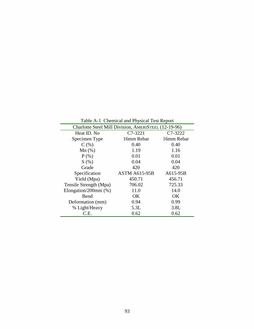
93

Table A-1 Chemical and Physical Test Report

Charlotte Steel Mill Division, AMERISTEEL (12-19-96) Heat ID. No C7-3221 C7-3222

Specimen Type 16mm Rebar 16mm Rebar C (%) 0.40 0.40

Mn (%) 1.19 1.16 P (%) 0.01 0.01 S (%) 0.04 0.04 Grade 420 420

Specification ASTM A615-95B A615-95B Yield (Mpa) 450.71 456.71

Tensile Strength (Mpa) 706.02 725.33 Elongation/200mm (%) 11.0 14.0

Bend OK OK Deformation (mm) 0.94 0.99

% Light/Heavy 5.3L 3.8L C.E. 0.62 0.62

94

Table A-2 Report of Chemical Analysis

Client’s Sample ID Blue Circle Type I Blue Circle Type I/II Material Type Cement Cement

CTL Sample ID 924713 924714

Analyte Weight (%) Weight (%) SiO2 20.82 20.74 Al2O3 4.27 4.69 Fe2O3 3.74 3.69 CaO 65.22 64.8 MgO 0.98 0.9 SO3 2.61 2.55

Na2O 0.06 0.07 K2O 0.21 0.26 TiO2 0.30 0.32 P2O5 0.22 0.20

Mn2O3 0.03 0.03 SrO 0.07 0.07

Loss on Ignition (950°C) 1.77 1.73 Total 100.31 100.04

Alkalis as Na2O 0.20 0.24

Insoluble Residue Free CaO

C3S 62 59 C2S 13 15 C3A 6 8

C4AF 11 11 ss(C4AF + C2F) --- ---

Date Analyzed: 04-30-97 Notes:

This analysis represents specifically the sample submitted. Oxide analysis by X-ray fluorescence spectrometry. Samples fused at 1000 degrees Celsius with Li2B4O7. Values for TiO2 and P2O5 are added to the Al2O3 when the compounds are calculated, in accordance with ASTM C 150. X-Ray Fluorescence oxide analysis meets the precision and accuracy requirements for rapid methods per ASTM C 114-94. Most recent re-qualification date is May 30, 1995.

95

Figure A-1 Batch Record – Control Specimen 1

Personnel: Michael C. Brown Date: 3/11/97John Haramis Ambient Temp (°F): 66

- Initial Mix Temp (°F): 71 Time: 10:43Final Mix Temp (°F): 71 Time: 11:02

Mix Description: Control Specimen 1

Base Mix Design (1 cu. yd.)Constituents Weight Volume Specifications ActualCoarse Aggregate 1445.0 lb 8.27 c.f. w/c 0.45 0.45 Fine Aggregate 1445.0 lb 8.77 c.f. Air 7.0% 6.0%Cement 635.0 lb 3.23 c.f. Slump (in.) 3.5 3.3 Water (w')* 310.0 lb 4.58 c.f. s.g. absorp.HRWR 63.5 oz 0.06 c.f. C.A. 2.80 0.85%Corrosion Inhibitor - gal - c.f. F.A. 2.64 0.83%Air 19.1 oz 1.89 c.f. Corr. Inh. % solids: 0%Total 3835 pcy 27.00 c.f. Water equivalent (lb) -

26.81 Batch Size 1.40 cu.ft.Constituents Type Design Mix Additional during mix Actual MixCoarse Aggregate #78, Acco 75.00 lb 0.00 lb 75.00 lbFine Aggregate Wytheville Sand 75.00 lb 0.00 lb 75.00 lbCement Type I, Blue Circle 32.96 lb 0.00 lb 32.96 lbWater (w')* tap (B'burg) 16.09 lb 0.01 lb 16.10 lbHRWR Daracem 98 ml (16) ml 82 mlAEA Daravair 29.3 ml - ml 29.3 mlCorrosion Inhibitor - oz - oz - ozTotal 205.20 lb (0.95) lb 204.25 lb* w' = total design mix water - liquid portion of corrosion inhibitor

Unit WeightCalculated (pcf) 142.04 Relative yield 97.3%Measured (pcf) 145.95 Calculated Yield 1.44 cu.ft.Actual Yield 1.40 cu.ft.

Compressive StrengthAge (days) Date lb area psi

3 03/14/97 50,500 12.57 4,020 7 03/18/97 56,000 12.57 4,460 28 04/08/97 77,000 12.57 6,130 28 04/08/97 76,500 12.57 6,090

365 03/11/98 97,500 12.57 7,760 365 03/11/98 102,000 12.57 8,120

Notes:

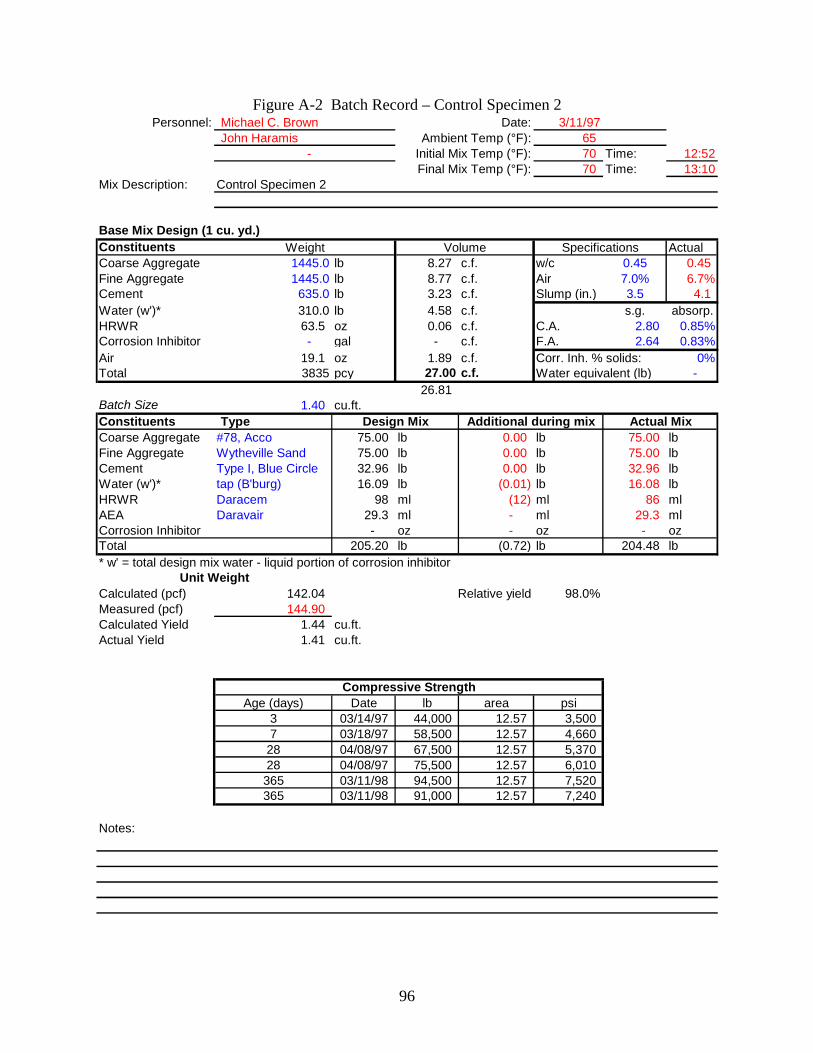
96

Figure A-2 Batch Record – Control Specimen 2 Personnel: Michael C. Brown Date: 3/11/97

John Haramis Ambient Temp (°F): 65 - Initial Mix Temp (°F): 70 Time: 12:52

Final Mix Temp (°F): 70 Time: 13:10Mix Description: Control Specimen 2

Base Mix Design (1 cu. yd.)Constituents Weight Volume Specifications ActualCoarse Aggregate 1445.0 lb 8.27 c.f. w/c 0.45 0.45 Fine Aggregate 1445.0 lb 8.77 c.f. Air 7.0% 6.7%Cement 635.0 lb 3.23 c.f. Slump (in.) 3.5 4.1 Water (w')* 310.0 lb 4.58 c.f. s.g. absorp.HRWR 63.5 oz 0.06 c.f. C.A. 2.80 0.85%Corrosion Inhibitor - gal - c.f. F.A. 2.64 0.83%Air 19.1 oz 1.89 c.f. Corr. Inh. % solids: 0%Total 3835 pcy 27.00 c.f. Water equivalent (lb) -

26.81 Batch Size 1.40 cu.ft.Constituents Type Design Mix Additional during mix Actual MixCoarse Aggregate #78, Acco 75.00 lb 0.00 lb 75.00 lbFine Aggregate Wytheville Sand 75.00 lb 0.00 lb 75.00 lbCement Type I, Blue Circle 32.96 lb 0.00 lb 32.96 lbWater (w')* tap (B'burg) 16.09 lb (0.01) lb 16.08 lbHRWR Daracem 98 ml (12) ml 86 mlAEA Daravair 29.3 ml - ml 29.3 mlCorrosion Inhibitor - oz - oz - ozTotal 205.20 lb (0.72) lb 204.48 lb* w' = total design mix water - liquid portion of corrosion inhibitor

Unit WeightCalculated (pcf) 142.04 Relative yield 98.0%Measured (pcf) 144.90 Calculated Yield 1.44 cu.ft.Actual Yield 1.41 cu.ft.

Compressive StrengthAge (days) Date lb area psi

3 03/14/97 44,000 12.57 3,500 7 03/18/97 58,500 12.57 4,660

28 04/08/97 67,500 12.57 5,370 28 04/08/97 75,500 12.57 6,010 365 03/11/98 94,500 12.57 7,520 365 03/11/98 91,000 12.57 7,240

Notes:

97

Figure A-3 Batch Record – Control Specimen 3 Personnel: Michael C. Brown Date: 3/11/97

John Haramis Ambient Temp (°F): 66 - Initial Mix Temp (°F): 70 Time: 14:23

Final Mix Temp (°F): 68 Time: 14:43Mix Description: Control Specimen 3

Base Mix Design (1 cu. yd.)Constituents Weight Volume Specifications ActualCoarse Aggregate 1445.0 lb 8.27 c.f. w/c 0.45 0.45 Fine Aggregate 1445.0 lb 8.77 c.f. Air 7.0% 6.6%Cement 635.0 lb 3.23 c.f. Slump (in.) 3.5 3.5 Water (w')* 310.0 lb 4.58 c.f. s.g. absorp.HRWR 63.5 oz 0.06 c.f. C.A. 2.80 0.85%Corrosion Inhibitor - gal - c.f. F.A. 2.64 0.83%Air 19.1 oz 1.89 c.f. Corr. Inh. % solids: 0%Total 3835 pcy 27.00 c.f. Water equivalent (lb) -

26.81 Batch Size 1.40 cu.ft.Constituents Type Design Mix Additional during mix Actual MixCoarse Aggregate #78, Acco 75.00 lb 0.00 lb 75.00 lbFine Aggregate Wytheville Sand 75.00 lb 0.00 lb 75.00 lbCement Type I, Blue Circle 32.96 lb 0.00 lb 32.96 lbWater (w')* tap (B'burg) 16.09 lb (0.01) lb 16.08 lbHRWR Daracem 98 ml (21) ml 77 mlAEA Daravair 29.3 ml - ml 29.3 mlCorrosion Inhibitor - oz - oz - ozTotal 205.20 lb (1.28) lb 203.92 lb* w' = total design mix water - liquid portion of corrosion inhibitor

Unit WeightCalculated (pcf) 142.04 Relative yield 98.2%Measured (pcf) 144.66 Calculated Yield 1.44 cu.ft.Actual Yield 1.41 cu.ft.

Compressive StrengthAge (days) Date lb area psi

3 03/14/97 47,500 12.57 3,780 7 03/18/97 53,500 12.57 4,260

28 04/08/97 74,000 12.57 5,890 28 04/08/97 76,000 12.57 6,050 365 03/11/98 95,500 12.57 7,600 365 03/11/98 97,500 12.57 7,760

Notes:

98

Figure A-4 Batch Record – DCI-S Specimen 1 Personnel: Michael C. Brown Date: 3/18/97

- Ambient Temp (°F): 66 - Initial Mix Temp (°F): 70 Time: 13:13

Final Mix Temp (°F): 70 Time: 13:33Mix Description: W.R.Grace - DCI-S Specimen 1

Base Mix Design (1 cu. yd.)Constituents Weight Volume Specifications ActualCoarse Aggregate 1445.0 lb 8.27 c.f. w/c 0.45 0.42 Fine Aggregate 1445.0 lb 8.77 c.f. Air 7.0% 5.5%Cement 635.0 lb 3.23 c.f. Slump (in.) 3.5 3.4 Water (w')* 289.4 lb 4.58 c.f. s.g. absorp.HRWR 63.5 oz 0.06 c.f. C.A. 2.80 0.85%Corrosion Inhibitor 3.00 gal 0.40 c.f. F.A. 2.64 0.83%Air 19.1 oz 1.89 c.f. Corr. Inh. 1.29 Total 3814 pcy 27.00 c.f. Corr. Inh. % solids: 36%

27.21 Water equivalent (lb) 20.66 Batch Size 1.40 cu.ft.Constituents Type Design Mix Additional during mix Actual MixCoarse Aggregate #78, Acco 75.00 lb 0.00 lb 75.00 lbFine Aggregate Wytheville Sand 75.00 lb 0.00 lb 75.00 lbCement Type I, Blue Circle 32.96 lb 0.00 lb 32.96 lbWater (w')* tap (B'burg) 15.02 lb 0.00 lb 15.02 lbHRWR Daracem 98 ml - ml 98 mlAEA Daravair 29.3 ml - ml 29.3 mlCorrosion Inhibitor DCI-S 590 ml - ml 590 mlTotal 200.01 lb 0.01 lb 200.03 lb* w' = total design mix water - liquid portion of corrosion inhibitor

Unit WeightCalculated (pcf) 141.27 Relative yield 96.4%Measured (pcf) 146.59 Calculated Yield 1.42 cu.ft.Actual Yield 1.36 cu.ft.

Compressive StrengthAge (days) Date lb area psi

3 03/21/97 60,500 12.57 4,810 7 03/25/97 78,000 12.57 6,210 28 04/15/97 91,000 12.57 7,240 28 04/15/97 91,000 12.57 7,240

365 03/18/98 115,000 12.57 9,150 365 03/18/98 114,500 12.57 9,110

Notes:Conferred with Dr. Weyers…agreed not to adjust air entrainment

99

Figure A-5 Batch Record – DCI-S Specimen 2 Personnel: Michael C. Brown Date: 3/18/97

- Ambient Temp (°F): 61 - Initial Mix Temp (°F): 68 Time: 14:50

Final Mix Temp (°F): 67 Time: 15:07Mix Description: W.R.Grace - DCI-S Specimen 2

Base Mix Design (1 cu. yd.)Constituents Weight Volume Specifications ActualCoarse Aggregate 1445.0 lb 8.27 c.f. w/c 0.45 0.42 Fine Aggregate 1445.0 lb 8.77 c.f. Air 7.0% 6.6%Cement 635.0 lb 3.23 c.f. Slump (in.) 3.5 4.0 Water (w')* 289.4 lb 4.58 c.f. s.g. absorp.HRWR 63.5 oz 0.06 c.f. C.A. 2.80 0.85%Corrosion Inhibitor 3.00 gal 0.40 c.f. F.A. 2.64 0.83%Air 19.1 oz 1.89 c.f. Corr. Inh. 1.29 Total 3814 pcy 27.00 c.f. Corr. Inh. % solids: 36%

27.21 Water equivalent (lb) 20.66 Batch Size 1.40 cu.ft.Constituents Type Design Mix Additional during mix Actual MixCoarse Aggregate #78, Acco 75.00 lb 0.00 lb 75.00 lbFine Aggregate Wytheville Sand 75.00 lb 0.00 lb 75.00 lbCement Type I, Blue Circle 32.96 lb 0.00 lb 32.96 lbWater (w')* tap (B'burg) 15.02 lb 0.00 lb 15.02 lbHRWR Daracem 98 ml - ml 98 mlAEA Daravair 29.3 ml - ml 29.3 mlCorrosion Inhibitor DCI-S 590 ml - ml 590 mlTotal 200.01 lb 0.01 lb 200.03 lb* w' = total design mix water - liquid portion of corrosion inhibitor

Unit WeightCalculated (pcf) 141.27 Relative yield 97.7%Measured (pcf) 144.57 Calculated Yield 1.42 cu.ft.Actual Yield 1.38 cu.ft.

Compressive StrengthAge (days) Date lb area psi

3 03/21/97 60,500 12.57 4,810 7 03/25/97 77,000 12.57 6,130 28 04/15/97 87,500 12.57 6,960 28 04/15/97 92,500 12.57 7,360

365 03/18/98 110,000 12.57 8,750 365 03/18/98 112,000 12.57 8,910

Notes:

100

Figure A-6 Batch Record – DCI-S Specimen 3 Personnel: Michael C. Brown Date: 3/18/97

- Ambient Temp (°F): 63 - Initial Mix Temp (°F): 69 Time: 16:35

Final Mix Temp (°F): 70 Time: 16:53Mix Description: W.R.Grace - DCI-S Specimen 3

Base Mix Design (1 cu. yd.)Constituents Weight Volume Specifications ActualCoarse Aggregate 1445.0 lb 8.27 c.f. w/c 0.45 0.42 Fine Aggregate 1445.0 lb 8.77 c.f. Air 7.0% 6.0%Cement 635.0 lb 3.23 c.f. Slump (in.) 3.5 - Water (w')* 289.4 lb 4.58 c.f. s.g. absorp.HRWR 63.5 oz 0.06 c.f. C.A. 2.80 0.85%Corrosion Inhibitor 3.00 gal 0.40 c.f. F.A. 2.64 0.83%Air 19.1 oz 1.89 c.f. Corr. Inh. 1.29 Total 3814 pcy 27.00 c.f. Corr. Inh. % solids: 36%

27.21 Water equivalent (lb) 20.66 Batch Size 1.40 cu.ft.Constituents Type Design Mix Additional during mix Actual MixCoarse Aggregate #78, Acco 75.00 lb 0.00 lb 75.00 lbFine Aggregate Wytheville Sand 75.00 lb 0.00 lb 75.00 lbCement Type I, Blue Circle 32.96 lb 0.00 lb 32.96 lbWater (w')* tap (B'burg) 15.02 lb 0.00 lb 15.02 lbHRWR Daracem 98 ml - ml 98 mlAEA Daravair 29.3 ml - ml 29.3 mlCorrosion Inhibitor DCI-S 590 ml - ml 590 mlTotal 200.01 lb 0.01 lb 200.03 lb* w' = total design mix water - liquid portion of corrosion inhibitor

Unit WeightCalculated (pcf) 141.27 Relative yield 96.8%Measured (pcf) 145.95 Calculated Yield 1.42 cu.ft.Actual Yield 1.37 cu.ft.

Compressive StrengthAge (days) Date lb area psi

3 03/21/97 58,500 12.57 4,660 7 03/25/97 77,000 12.57 6,130 28 04/15/97 87,000 12.57 6,920 28 04/15/97 89,500 12.57 7,120

365 03/18/98 114,000 12.57 9,070 365 03/18/98 107,000 12.57 8,510

Notes:

101

Figure A-7 Batch Record – Rheocrete 222+ Specimen 1 Personnel: Michael C. Brown Date: 3/25/97

John Haramis Ambient Temp (°F): 63 - Initial Mix Temp (°F): 67 Time: 11:36

Final Mix Temp (°F): 66 Time: 12:08Mix Description: Master Builders - Rheocrete 222+ Specimen 1

Base Mix Design (1 cu. yd.)Constituents Weight Volume Specifications ActualCoarse Aggregate 1445.0 lb 8.27 c.f. w/c 0.45 0.44 Fine Aggregate 1445.0 lb 8.77 c.f. Air 7.0% 5.7%Cement 635.0 lb 3.23 c.f. Slump (in.) 3.5 3.5 Water (w')* 301.6 lb 4.58 c.f. s.g. absorp.HRWR 63.5 oz 0.06 c.f. C.A. 2.80 0.85%Corrosion Inhibitor 1.00 gal 0.13 c.f. F.A. 2.64 0.83%Air 28.6 oz 1.89 c.f. Corr. Inh. 1.29 Total 3827 pcy 27.00 c.f. Corr. Inh. % solids: 22%

26.94 Water equivalent (lb) 8.39 Batch Size 1.40 cu.ft.Constituents Type Design Mix Additional during mix Actual MixCoarse Aggregate #78, Acco 75.00 lb 0.00 lb 75.00 lbFine Aggregate Wytheville Sand 75.00 lb 0.00 lb 75.00 lbCement Type I, Blue Circle 32.96 lb 0.00 lb 32.96 lbWater (w')* tap (B'burg) 15.66 lb 0.00 lb 15.66 lbHRWR Rheobuild 1000 98 ml (20) ml 78 mlAEA MB-VR 43.9 ml 29.0 ml 72.9 mlCorrosion Inhibitor Rheocrete 222+ 197 ml - ml 197 mlTotal 199.57 lb 0.04 lb 199.61 lb* w' = total design mix water - liquid portion of corrosion inhibitor

Unit WeightCalculated (pcf) 141.73 Relative yield 96.9%Measured (pcf) 146.27 Calculated Yield 1.41 cu.ft.Actual Yield 1.36 cu.ft.

Compressive StrengthAge (days) Date lb area psi

3 03/28/97 49,500 12.57 3,940 7 04/01/97 60,500 12.57 4,810

28 04/22/97 75,500 12.57 6,010 28 04/22/97 73,000 12.57 5,810 365 03/25/98 95,500 12.57 7,600 365 03/25/98 88,000 12.57 7,000

Notes:

102

Figure A-8 Batch Record - Rheocrete 222+ Specimen 2 Personnel: Michael C. Brown Date: 3/25/97

John Haramis Ambient Temp (°F): 63 - Initial Mix Temp (°F): 66 Time: 13:21

Final Mix Temp (°F): 67 Time: 13:36Mix Description: Master Builders - Rheocrete 222+ Specimen 2

Base Mix Design (1 cu. yd.)Constituents Weight Volume Specifications ActualCoarse Aggregate 1445.0 lb 8.27 c.f. w/c 0.45 0.44 Fine Aggregate 1445.0 lb 8.77 c.f. Air 7.0% 6.8%Cement 635.0 lb 3.23 c.f. Slump (in.) 3.5 5.5 Water (w')* 301.6 lb 4.58 c.f. s.g. absorp.HRWR 63.5 oz 0.06 c.f. C.A. 2.80 0.85%Corrosion Inhibitor 1.00 gal 0.13 c.f. F.A. 2.64 0.83%Air 28.6 oz 1.89 c.f. Corr. Inh. 1.29 Total 3827 pcy 27.00 c.f. Corr. Inh. % solids: 22%

26.94 Water equivalent (lb) 8.39 Batch Size 1.40 cu.ft.Constituents Type Design Mix Additional during mix Actual MixCoarse Aggregate #78, Acco 75.00 lb 0.00 lb 75.00 lbFine Aggregate Wytheville Sand 75.00 lb 0.00 lb 75.00 lbCement Type I, Blue Circle 32.96 lb 0.00 lb 32.96 lbWater (w')* tap (B'burg) 15.66 lb 0.00 lb 15.66 lbHRWR Rheobuild 1000 98 ml (15) ml 83 mlAEA MB-VR 43.9 ml 63.0 ml 106.9 mlCorrosion Inhibitor Rheocrete 222+ 197 ml - ml 197 mlTotal 199.57 lb 0.15 lb 199.72 lb* w' = total design mix water - liquid portion of corrosion inhibitor

Unit WeightCalculated (pcf) 141.73 Relative yield 98.8%Measured (pcf) 143.44 Calculated Yield 1.41 cu.ft.Actual Yield 1.39 cu.ft.

Compressive StrengthAge (days) Date lb area psi

3 03/28/97 44,000 12.57 3,500 7 04/01/97 58,000 12.57 4,620

28 04/22/97 67,500 12.57 5,370 28 04/22/97 63,500 12.57 5,050 365 03/25/98 88,000 12.57 7,000 365 03/25/98 86,000 12.57 6,840

Notes:

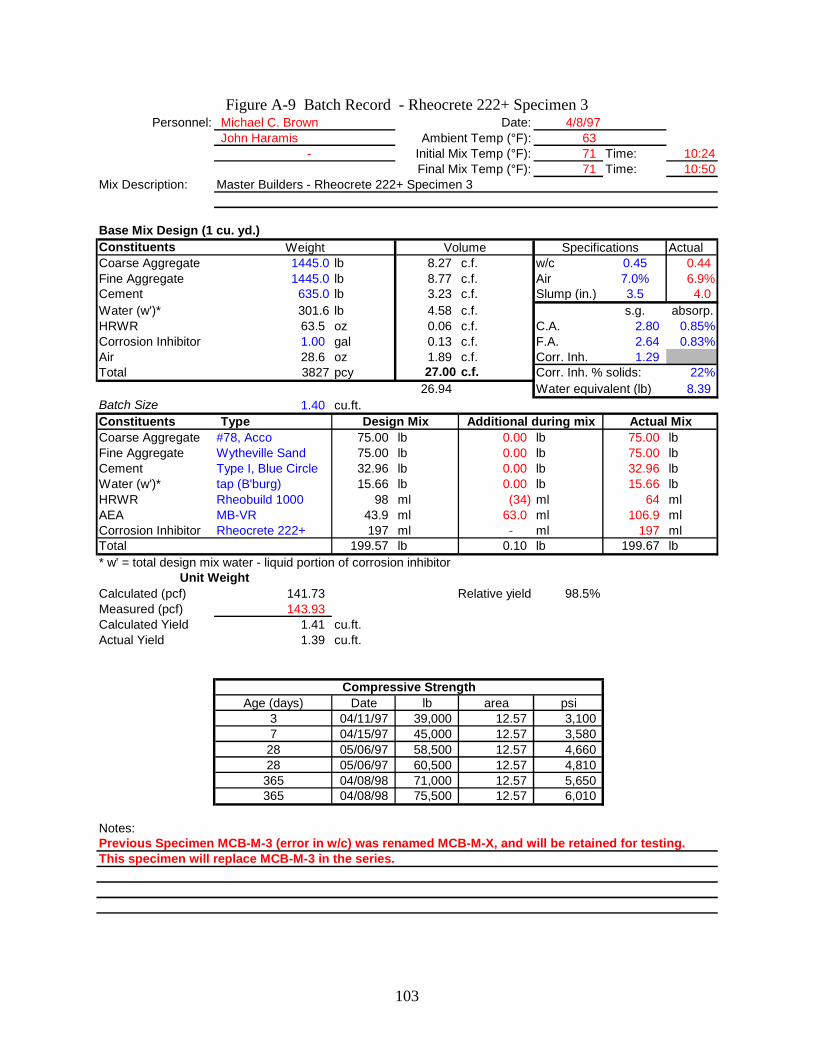
103

Figure A-9 Batch Record - Rheocrete 222+ Specimen 3 Personnel: Michael C. Brown Date: 4/8/97

John Haramis Ambient Temp (°F): 63 - Initial Mix Temp (°F): 71 Time: 10:24

Final Mix Temp (°F): 71 Time: 10:50Mix Description: Master Builders - Rheocrete 222+ Specimen 3

Base Mix Design (1 cu. yd.)Constituents Weight Volume Specifications ActualCoarse Aggregate 1445.0 lb 8.27 c.f. w/c 0.45 0.44 Fine Aggregate 1445.0 lb 8.77 c.f. Air 7.0% 6.9%Cement 635.0 lb 3.23 c.f. Slump (in.) 3.5 4.0 Water (w')* 301.6 lb 4.58 c.f. s.g. absorp.HRWR 63.5 oz 0.06 c.f. C.A. 2.80 0.85%Corrosion Inhibitor 1.00 gal 0.13 c.f. F.A. 2.64 0.83%Air 28.6 oz 1.89 c.f. Corr. Inh. 1.29 Total 3827 pcy 27.00 c.f. Corr. Inh. % solids: 22%

26.94 Water equivalent (lb) 8.39 Batch Size 1.40 cu.ft.Constituents Type Design Mix Additional during mix Actual MixCoarse Aggregate #78, Acco 75.00 lb 0.00 lb 75.00 lbFine Aggregate Wytheville Sand 75.00 lb 0.00 lb 75.00 lbCement Type I, Blue Circle 32.96 lb 0.00 lb 32.96 lbWater (w')* tap (B'burg) 15.66 lb 0.00 lb 15.66 lbHRWR Rheobuild 1000 98 ml (34) ml 64 mlAEA MB-VR 43.9 ml 63.0 ml 106.9 mlCorrosion Inhibitor Rheocrete 222+ 197 ml - ml 197 mlTotal 199.57 lb 0.10 lb 199.67 lb* w' = total design mix water - liquid portion of corrosion inhibitor

Unit WeightCalculated (pcf) 141.73 Relative yield 98.5%Measured (pcf) 143.93 Calculated Yield 1.41 cu.ft.Actual Yield 1.39 cu.ft.

Compressive StrengthAge (days) Date lb area psi

3 04/11/97 39,000 12.57 3,100 7 04/15/97 45,000 12.57 3,580

28 05/06/97 58,500 12.57 4,660 28 05/06/97 60,500 12.57 4,810 365 04/08/98 71,000 12.57 5,650 365 04/08/98 75,500 12.57 6,010

Notes:Previous Specimen MCB-M-3 (error in w/c) was renamed MCB-M-X, and will be retained for testing.This specimen will replace MCB-M-3 in the series.

104

Figure A-10 Batch Record - FerroGard 901 Specimen 1 Personnel: Michael C. Brown Date: 4/1/97

John Haramis Ambient Temp (°F): 68 - Initial Mix Temp (°F): 70 Time: 0:00

Final Mix Temp (°F): 68 Time: 0:00Mix Description: Sika Ferrogard 901 - Specimen 1

Base Mix Design (1 cu. yd.)Constituents Weight Volume Specifications ActualCoarse Aggregate 1445.0 lb 8.27 c.f. w/c 0.45 0.42 Fine Aggregate 1445.0 lb 8.77 c.f. Air 7.0% 5.9%Cement 635.0 lb 3.23 c.f. Slump (in.) 3.5 4.3 Water (w')* 292.0 lb 4.58 c.f. s.g. absorp.HRWR 63.5 oz 0.06 c.f. C.A. 2.80 0.85%Corrosion Inhibitor 2.00 gal 0.27 c.f. F.A. 2.64 0.83%Air 19.1 oz 1.89 c.f. Corr. Inh. 1.29 Total 3817 pcy 27.00 c.f. Corr. Inh. % solids: 16%

27.07 Water equivalent (lb) 18.08 Batch Size 1.40 cu.ft.Constituents Type Design Mix Additional during mix Actual MixCoarse Aggregate #78, Acco 75.00 lb 0.00 lb 75.00 lbFine Aggregate Wytheville Sand 75.00 lb 0.00 lb 75.00 lbCement Type I, Blue Circle 32.96 lb 0.00 lb 32.96 lbWater (w')* tap (B'burg) 15.15 lb (0.01) lb 15.14 lbHRWR Sikament 86 (HRWR 98 ml (52) ml 46 mlAEA Sika AER (AEA) SA0 29.3 ml - ml 29.3 mlCorrosion Inhibitor Ferrogard 901 393 ml - ml 393 mlTotal 199.59 lb (0.15) lb 199.44 lb* w' = total design mix water - liquid portion of corrosion inhibitor

Unit WeightCalculated (pcf) 141.37 Relative yield 97.0%Measured (pcf) 145.78 Calculated Yield 1.41 cu.ft.Actual Yield 1.37 cu.ft.

Compressive StrengthAge (days) Date lb area psi

3 04/04/97 54,500 12.57 4,340 7 04/08/97 70,500 12.57 5,610 28 04/29/97 90,000 12.57 7,160 28 04/29/97 92,500 12.57 7,360

365 04/01/98 113,000 12.57 8,990 365 04/01/98 116,500 12.57 9,270

Notes:

105

Figure A-11 Batch Record - FerroGard 901 Specimen 2 Personnel: Michael C. Brown Date: 4/1/97

John Haramis Ambient Temp (°F): 67 - Initial Mix Temp (°F): 68 Time: 12:56

Final Mix Temp (°F): 68 Time: 13:19Mix Description: Sika Ferrogard 901 - Specimen 2

Base Mix Design (1 cu. yd.)Constituents Weight Volume Specifications ActualCoarse Aggregate 1445.0 lb 8.27 c.f. w/c 0.45 0.42 Fine Aggregate 1445.0 lb 8.77 c.f. Air 7.0% 5.6%Cement 635.0 lb 3.23 c.f. Slump (in.) 3.5 3.5 Water (w')* 292.0 lb 4.58 c.f. s.g. absorp.HRWR 63.5 oz 0.06 c.f. C.A. 2.80 0.85%Corrosion Inhibitor 2.00 gal 0.27 c.f. F.A. 2.64 0.83%Air 19.1 oz 1.89 c.f. Corr. Inh. 1.29 Total 3817 pcy 27.00 c.f. Corr. Inh. % solids: 16%

27.07 Water equivalent (lb) 18.08 Batch Size 1.40 cu.ft.Constituents Type Design Mix Additional during mix Actual MixCoarse Aggregate #78, Acco 75.00 lb 0.00 lb 75.00 lbFine Aggregate Wytheville Sand 75.00 lb 0.00 lb 75.00 lbCement Type I, Blue Circle 32.96 lb 0.00 lb 32.96 lbWater (w')* tap (B'burg) 15.15 lb 0.01 lb 15.16 lbHRWR Sikament 86 (HRWR 98 ml (67) ml 31 mlAEA Sika AER (AEA) SA0 29.3 ml - ml 29.3 mlCorrosion Inhibitor Ferrogard 901 393 ml - ml 393 mlTotal 199.59 lb (0.17) lb 199.41 lb* w' = total design mix water - liquid portion of corrosion inhibitor

Unit WeightCalculated (pcf) 141.37 Relative yield 96.9%Measured (pcf) 145.95 Calculated Yield 1.41 cu.ft.Actual Yield 1.37 cu.ft.

Compressive StrengthAge (days) Date lb area psi

3 04/04/97 57,000 12.57 4,540 7 04/08/97 71,500 12.57 5,690 28 04/29/97 91,500 12.57 7,280 28 04/29/97 92,000 12.57 7,320

365 04/01/98 112,500 12.57 8,950 365 04/01/98 112,500 12.57 8,950

Notes:

106

Figure A-12 Batch Record - FerroGard 901 Specimen 3 Personnel: Michael C. Brown Date: 4/1/97

John Haramis Ambient Temp (°F): 68 - Initial Mix Temp (°F): 69 Time: 14:09

Final Mix Temp (°F): 68 Time: 14:25Mix Description: Sika Ferrogard 901 - Specimen 3

Base Mix Design (1 cu. yd.)Constituents Weight Volume Specifications ActualCoarse Aggregate 1445.0 lb 8.27 c.f. w/c 0.45 0.42 Fine Aggregate 1445.0 lb 8.77 c.f. Air 7.0% 5.5%Cement 635.0 lb 3.23 c.f. Slump (in.) 3.5 3.1 Water (w')* 292.0 lb 4.58 c.f. s.g. absorp.HRWR 63.5 oz 0.06 c.f. C.A. 2.80 0.85%Corrosion Inhibitor 2.00 gal 0.27 c.f. F.A. 2.64 0.83%Air 19.1 oz 1.89 c.f. Corr. Inh. 1.29 Total 3817 pcy 27.00 c.f. Corr. Inh. % solids: 16%

27.07 Water equivalent (lb) 18.08 Batch Size 1.40 cu.ft.Constituents Type Design Mix Additional during mix Actual MixCoarse Aggregate #78, Acco 75.00 lb 0.00 lb 75.00 lbFine Aggregate Wytheville Sand 75.00 lb 0.00 lb 75.00 lbCement Type I, Blue Circle 32.96 lb 0.00 lb 32.96 lbWater (w')* tap (B'burg) 15.15 lb 0.01 lb 15.16 lbHRWR Sikament 86 (HRWR 98 ml (69) ml 29 mlAEA Sika AER (AEA) SA0 29.3 ml - ml 29.3 mlCorrosion Inhibitor Ferrogard 901 393 ml - ml 393 mlTotal 199.59 lb (0.18) lb 199.41 lb* w' = total design mix water - liquid portion of corrosion inhibitor

Unit WeightCalculated (pcf) 141.37 Relative yield 96.9%Measured (pcf) 145.95 Calculated Yield 1.41 cu.ft.Actual Yield 1.37 cu.ft.

Compressive StrengthAge (days) Date lb area psi

3 04/04/97 55,500 12.57 4,420 7 04/08/97 70,000 12.57 5,570 28 04/29/97 90,000 12.57 7,160 28 04/29/97 90,000 12.57 7,160

365 04/01/98 112,500 12.57 8,950 365 04/01/98 110,000 12.57 8,750

Notes:

107

Figure A-13 Batch Record - Catexol 1000 Specimen 1 Personnel: Michael C. Brown Date: 5/20/97

John Haramis Ambient Temp (°F): 71 Ryan Weyers Initial Mix Temp (°F): 74 Time: 11:15

Final Mix Temp (°F): 71 Time: 11:30Mix Description: Axim Concrete Products - Catexol 1000 C.I. - Specimen 1 (rebatch)

Base Mix Design (1 cu. yd.)Constituents Weight Volume Specifications ActualCoarse Aggregate 1445.0 lb 8.27 c.f. w/c 0.45 0.43 Fine Aggregate 1445.0 lb 8.77 c.f. Air 7.0% 7.2%Cement 635.0 lb 3.23 c.f. Slump (in.) 3.5 3.3 Water (w')* 294.9 lb 4.58 c.f. s.g. absorp.HRWR 63.5 oz 0.06 c.f. C.A. 2.80 0.85%Corrosion Inhibitor 3.00 gal 0.40 c.f. F.A. 2.64 0.83%Air 19.1 oz 1.89 c.f. Corr. Inh. 1.10 Total 3820 pcy 27.00 c.f. Corr. Inh. % solids: 45%

27.21 Water equivalent (lb) 15.14 Batch Size 1.40 cu.ft.Constituents Type Design Mix Additional during mix Actual MixCoarse Aggregate #78, Acco 75.00 lb 0.00 lb 75.00 lbFine Aggregate Wytheville Sand 75.00 lb 0.00 lb 75.00 lbCement Type I, Blue Circle 32.96 lb 0.00 lb 32.96 lbWater (w')* tap (B'burg) 15.31 lb 0.01 lb 15.32 lbHRWR Catexol 1000 SP-MN 98 ml (58) ml 40 mlAEA Catexol A.E. 29.3 ml - ml 29.3 mlCorrosion Inhibitor Catexol 1000 C.I. 590 ml - ml 590 mlTotal 200.00 lb (0.11) lb 199.88 lb* w' = total design mix water - liquid portion of corrosion inhibitor

Unit WeightCalculated (pcf) 141.48 Relative yield 99.8%Measured (pcf) 141.75 Calculated Yield 1.41 cu.ft.Actual Yield 1.41 cu.ft.

Compressive StrengthAge (days) Date lb area psi

3 05/23/97 37,500 12.57 2,980 7 05/27/97 47,000 12.57 3,740

28 06/17/97 54,000 12.57 4,300 28 06/17/97 56,500 12.57 4,500 365 05/20/98 67,500 12.57 5,370 365 05/20/98 67,500 12.57 5,370

Notes:

108

Figure A-14 Batch Record - Catexol 1000 Specimen 2 Personnel: Michael C. Brown Date: 5/20/97

John Haramis Ambient Temp (°F): 69 Ryan Weyers Initial Mix Temp (°F): 73 Time: 12:18

Final Mix Temp (°F): 73 Time: 12:41Mix Description: Axim Concrete Products - Catexol 1000 C.I. - Specimen 2 (rebatch)

Base Mix Design (1 cu. yd.)Constituents Weight Volume Specifications ActualCoarse Aggregate 1445.0 lb 8.27 c.f. w/c 0.45 0.39 Fine Aggregate 1445.0 lb 8.77 c.f. Air 7.0% 7.2%Cement 635.0 lb 3.23 c.f. Slump (in.) 3.5 3.0 Water (w')* 294.9 lb 4.58 c.f. s.g. absorp.HRWR 63.5 oz 0.06 c.f. C.A. 2.80 0.85%Corrosion Inhibitor 3.00 gal 0.40 c.f. F.A. 2.64 0.83%Air 19.1 oz 1.89 c.f. Corr. Inh. 1.10 Total 3820 pcy 27.00 c.f. Corr. Inh. % solids: 45%

27.21 Water equivalent (lb) 15.14 Batch Size 1.40 cu.ft.Constituents Type Design Mix Additional during mix Actual MixCoarse Aggregate #78, Acco 75.00 lb 0.00 lb 75.00 lbFine Aggregate Wytheville Sand 75.00 lb 0.00 lb 75.00 lbCement Type I, Blue Circle 32.96 lb 3.00 lb 35.96 lbWater (w')* tap (B'burg) 15.31 lb 0.01 lb 15.32 lbHRWR Catexol 1000 SP-MN 98 ml (61) ml 37 mlAEA Catexol A.E. 29.3 ml (2.0) ml 27.3 mlCorrosion Inhibitor Catexol 1000 C.I. 590 ml - ml 590 mlTotal 200.00 lb 2.87 lb 202.87 lb* w' = total design mix water - liquid portion of corrosion inhibitor

Unit WeightCalculated (pcf) 141.48 Relative yield 99.4%Measured (pcf) 142.32 Calculated Yield 1.41 cu.ft.Actual Yield 1.43 cu.ft.

Compressive StrengthAge (days) Date lb area psi

3 05/23/97 36,000 12.57 2,860 7 05/27/97 46,000 12.57 3,660

28 06/17/97 56,500 12.57 4,500 28 06/17/97 53,500 12.57 4,260 365 05/20/98 67,000 12.57 5,330 365 05/20/98 67,500 12.57 5,370

Notes:

109

Figure A-15 Batch Record - Catexol 1000 Specimen 3 Personnel: Michael C. Brown Date: 5/20/97

John Haramis Ambient Temp (°F): 70 Ryan Weyers Initial Mix Temp (°F): 75 Time: 13:36

Final Mix Temp (°F): 75 Time: 13:45Mix Description: Axim Concrete Products - Catexol 1000 C.I. - Specimen 3 (rebatch)

Base Mix Design (1 cu. yd.)Constituents Weight Volume Specifications ActualCoarse Aggregate 1445.0 lb 8.27 c.f. w/c 0.45 0.43 Fine Aggregate 1445.0 lb 8.77 c.f. Air 7.0% 7.4%Cement 635.0 lb 3.23 c.f. Slump (in.) 3.5 3.5 Water (w')* 294.9 lb 4.58 c.f. s.g. absorp.HRWR 63.5 oz 0.06 c.f. C.A. 2.80 0.85%Corrosion Inhibitor 3.00 gal 0.40 c.f. F.A. 2.64 0.83%Air 19.1 oz 1.89 c.f. Corr. Inh. 1.10 Total 3820 pcy 27.00 c.f. Corr. Inh. % solids: 45%

27.21 Water equivalent (lb) 15.14 Batch Size 1.40 cu.ft.Constituents Type Design Mix Additional during mix Actual MixCoarse Aggregate #78, Acco 75.00 lb 0.00 lb 75.00 lbFine Aggregate Wytheville Sand 75.00 lb 0.00 lb 75.00 lbCement Type I, Blue Circle 32.96 lb 0.00 lb 32.96 lbWater (w')* tap (B'burg) 15.31 lb 0.01 lb 15.32 lbHRWR Catexol 1000 SP-MN 98 ml (52) ml 46 mlAEA Catexol A.E. 29.3 ml (4.0) ml 25.3 mlCorrosion Inhibitor Catexol 1000 C.I. 590 ml - ml 590 mlTotal 200.00 lb (0.11) lb 199.89 lb* w' = total design mix water - liquid portion of corrosion inhibitor

Unit WeightCalculated (pcf) 141.48 Relative yield 99.8%Measured (pcf) 141.75 Calculated Yield 1.41 cu.ft.Actual Yield 1.41 cu.ft.

Compressive StrengthAge (days) Date lb area psi

3 05/23/97 38,500 12.57 3,060 7 05/27/97 45,000 12.57 3,580

28 06/17/97 52,000 12.57 4,140 28 06/17/97 54,500 12.57 4,340 365 05/20/98 66,500 12.57 5,290 365 05/20/98 68,000 12.57 5,410

Notes:

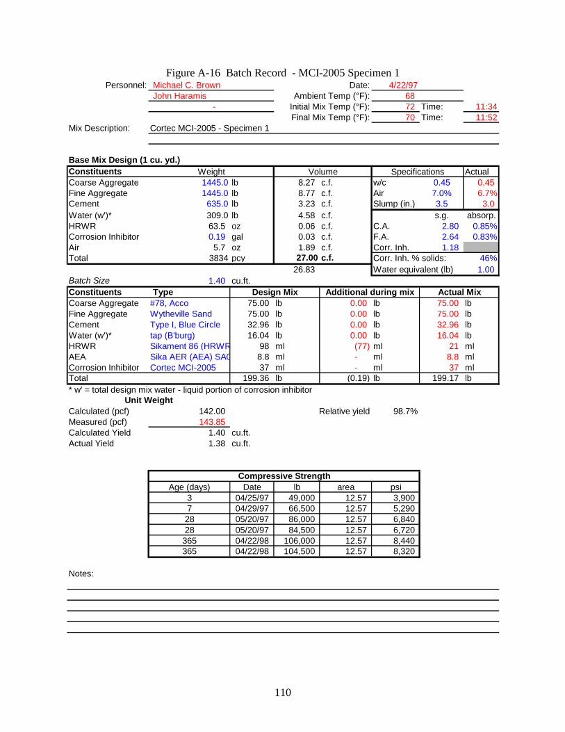
110

Figure A-16 Batch Record - MCI-2005 Specimen 1 Personnel: Michael C. Brown Date: 4/22/97

John Haramis Ambient Temp (°F): 68 - Initial Mix Temp (°F): 72 Time: 11:34

Final Mix Temp (°F): 70 Time: 11:52Mix Description: Cortec MCI-2005 - Specimen 1

Base Mix Design (1 cu. yd.)Constituents Weight Volume Specifications ActualCoarse Aggregate 1445.0 lb 8.27 c.f. w/c 0.45 0.45 Fine Aggregate 1445.0 lb 8.77 c.f. Air 7.0% 6.7%Cement 635.0 lb 3.23 c.f. Slump (in.) 3.5 3.0 Water (w')* 309.0 lb 4.58 c.f. s.g. absorp.HRWR 63.5 oz 0.06 c.f. C.A. 2.80 0.85%Corrosion Inhibitor 0.19 gal 0.03 c.f. F.A. 2.64 0.83%Air 5.7 oz 1.89 c.f. Corr. Inh. 1.18 Total 3834 pcy 27.00 c.f. Corr. Inh. % solids: 46%

26.83 Water equivalent (lb) 1.00 Batch Size 1.40 cu.ft.Constituents Type Design Mix Additional during mix Actual MixCoarse Aggregate #78, Acco 75.00 lb 0.00 lb 75.00 lbFine Aggregate Wytheville Sand 75.00 lb 0.00 lb 75.00 lbCement Type I, Blue Circle 32.96 lb 0.00 lb 32.96 lbWater (w')* tap (B'burg) 16.04 lb 0.00 lb 16.04 lbHRWR Sikament 86 (HRWR 98 ml (77) ml 21 mlAEA Sika AER (AEA) SA0 8.8 ml - ml 8.8 mlCorrosion Inhibitor Cortec MCI-2005 37 ml - ml 37 mlTotal 199.36 lb (0.19) lb 199.17 lb* w' = total design mix water - liquid portion of corrosion inhibitor

Unit WeightCalculated (pcf) 142.00 Relative yield 98.7%Measured (pcf) 143.85 Calculated Yield 1.40 cu.ft.Actual Yield 1.38 cu.ft.

Compressive StrengthAge (days) Date lb area psi

3 04/25/97 49,000 12.57 3,900 7 04/29/97 66,500 12.57 5,290 28 05/20/97 86,000 12.57 6,840 28 05/20/97 84,500 12.57 6,720

365 04/22/98 106,000 12.57 8,440 365 04/22/98 104,500 12.57 8,320

Notes:

111

Figure A-17 Batch Record - MCI-2005 Specimen 2 Personnel: Michael C. Brown Date: 4/22/97

John Haramis Ambient Temp (°F): 68 - Initial Mix Temp (°F): 72 Time: 12:38

Final Mix Temp (°F): 70 Time: 12:56Mix Description: Cortec MCI-2005 - Specimen 2

Base Mix Design (1 cu. yd.)Constituents Weight Volume Specifications ActualCoarse Aggregate 1445.0 lb 8.27 c.f. w/c 0.45 0.45 Fine Aggregate 1445.0 lb 8.77 c.f. Air 7.0% 7.0%Cement 635.0 lb 3.23 c.f. Slump (in.) 3.5 3.5 Water (w')* 309.0 lb 4.58 c.f. s.g. absorp.HRWR 63.5 oz 0.06 c.f. C.A. 2.80 0.85%Corrosion Inhibitor 0.19 gal 0.03 c.f. F.A. 2.64 0.83%Air 5.7 oz 1.89 c.f. Corr. Inh. 1.18 Total 3834 pcy 27.00 c.f. Corr. Inh. % solids: 46%

26.83 Water equivalent (lb) 1.00 Batch Size 1.40 cu.ft.Constituents Type Design Mix Additional during mix Actual MixCoarse Aggregate #78, Acco 75.00 lb 0.00 lb 75.00 lbFine Aggregate Wytheville Sand 75.00 lb 0.00 lb 75.00 lbCement Type I, Blue Circle 32.96 lb 0.00 lb 32.96 lbWater (w')* tap (B'burg) 16.04 lb 0.00 lb 16.04 lbHRWR Sikament 86 (HRWR 98 ml (67) ml 31 mlAEA Sika AER (AEA) SA0 8.8 ml - ml 8.8 mlCorrosion Inhibitor Cortec MCI-2005 37 ml - ml 37 mlTotal 199.36 lb (0.16) lb 199.20 lb* w' = total design mix water - liquid portion of corrosion inhibitor

Unit WeightCalculated (pcf) 142.00 Relative yield 99.2%Measured (pcf) 143.20 Calculated Yield 1.40 cu.ft.Actual Yield 1.39 cu.ft.

Compressive StrengthAge (days) Date lb area psi

3 04/25/97 50,000 12.57 3,980 7 04/29/97 65,500 12.57 5,210 28 05/20/97 84,000 12.57 6,680 28 05/20/97 80,000 12.57 6,370

365 04/22/98 103,000 12.57 8,200 365 04/22/98 105,500 12.57 8,400

Notes:

112

Figure A-18 Batch Record – MCI-2005 Specimen 3

Personnel: Michael C. Brown Date: 4/22/97John Haramis Ambient Temp (°F): 65

- Initial Mix Temp (°F): 71 Time: 13:41Final Mix Temp (°F): 70 Time: 14:10

Mix Description: Cortec MCI-2005 - Specimen 3

Base Mix Design (1 cu. yd.)Constituents Weight Volume Specifications ActualCoarse Aggregate 1445.0 lb 8.27 c.f. w/c 0.45 0.45 Fine Aggregate 1445.0 lb 8.77 c.f. Air 7.0% 7.2%Cement 635.0 lb 3.23 c.f. Slump (in.) 3.5 4.0 Water (w')* 309.0 lb 4.58 c.f. s.g. absorp.HRWR 63.5 oz 0.06 c.f. C.A. 2.80 0.85%Corrosion Inhibitor 0.19 gal 0.03 c.f. F.A. 2.64 0.83%Air 5.7 oz 1.89 c.f. Corr. Inh. 1.18 Total 3834 pcy 27.00 c.f. Corr. Inh. % solids: 46%

26.83 Water equivalent (lb) 1.00 Batch Size 1.40 cu.ft.Constituents Type Design Mix Additional during mix Actual MixCoarse Aggregate #78, Acco 75.00 lb 0.00 lb 75.00 lbFine Aggregate Wytheville Sand 75.00 lb 0.00 lb 75.00 lbCement Type I, Blue Circle 32.96 lb 0.00 lb 32.96 lbWater (w')* tap (B'burg) 16.04 lb 0.00 lb 16.04 lbHRWR Sikament 86 (HRWR 98 ml (70) ml 28 mlAEA Sika AER (AEA) SA0 8.8 ml - ml 8.8 mlCorrosion Inhibitor Cortec MCI-2005 37 ml - ml 37 mlTotal 199.36 lb (0.17) lb 199.19 lb* w' = total design mix water - liquid portion of corrosion inhibitor

Unit WeightCalculated (pcf) 142.00 Relative yield 99.5%Measured (pcf) 142.72 Calculated Yield 1.40 cu.ft.Actual Yield 1.40 cu.ft.

Compressive StrengthAge (days) Date lb area psi

3 04/25/97 47,500 12.57 3,780 7 04/29/97 66,000 12.57 5,250 28 05/20/97 85,000 12.57 6,760 28 05/20/97 83,500 12.57 6,640

365 04/22/98 106,500 12.57 8,480 365 04/22/98 104,000 12.57 8,280

Notes:

113

B - HEAT OF HYDRATION

114

Control SpecimensHeat of Hydration - Average with 95% Confidence Intervals

0

5

10

15

20

25

30

35

40

45

0 4 8 12 16 20 24 28 32 36 40 44Time (hours)

Tem

pera

ture

(°C

)

Control-Ave

Ambient

Figure B-1 Heat of Hydration – Control

DCI-S Specimens Heat of Hydration - Average with 95% Confidence Intervals

0

5

10

15

20

25

30

35

40

45

0 4 8 12 16 20 24 28 32 36 40 44Time (hours)

Tem

pera

ture

(°C

)

DCI - Ave

Ambient

Figure B-2 Heat of Hydration – DCI-S

115

Rheocrete 222+ Specimens Heat of Hydration - Average with 95% Confidence Intervals*

0

5

10

15

20

25

30

35

40

45

0 4 8 12 16 20 24 28 32 36 40 44Time (hours)

Tem

pera

ture

(°C

)

Rheocrete 222+ - Ave

Ambient

* Average does not include MCB-M-X

Figure B-3 Heat of Hydration – Rheocrete 222+

FerroGard 901 Specimens Heat of Hydration - Average with 95% Confidence Intervals

0

5

10

15

20

25

30

35

40

45

0 4 8 12 16 20 24 28 32 36 40 44Time (hours)

Tem

pera

ture

(°C

)

FerroGard 901 - Ave

Ambient

Figure B-4 Heat of Hydration – FerroGard 901

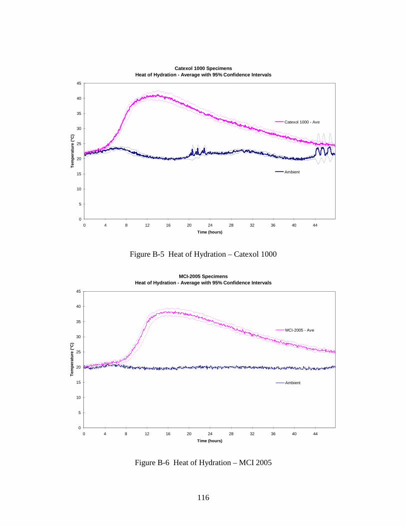
116

Catexol 1000 Specimens Heat of Hydration - Average with 95% Confidence Intervals

0

5

10

15

20

25

30

35

40

45

0 4 8 12 16 20 24 28 32 36 40 44Time (hours)

Tem

pera

ture

(°C

)

Catexol 1000 - Ave

Ambient

Figure B-5 Heat of Hydration – Catexol 1000

MCI-2005 Specimens Heat of Hydration - Average with 95% Confidence Intervals

0

5

10

15

20

25

30

35

40

45

0 4 8 12 16 20 24 28 32 36 40 44Time (hours)

Tem

pera

ture

(°C

)

MCI-2005 - Ave

Ambient

Figure B-6 Heat of Hydration – MCI 2005

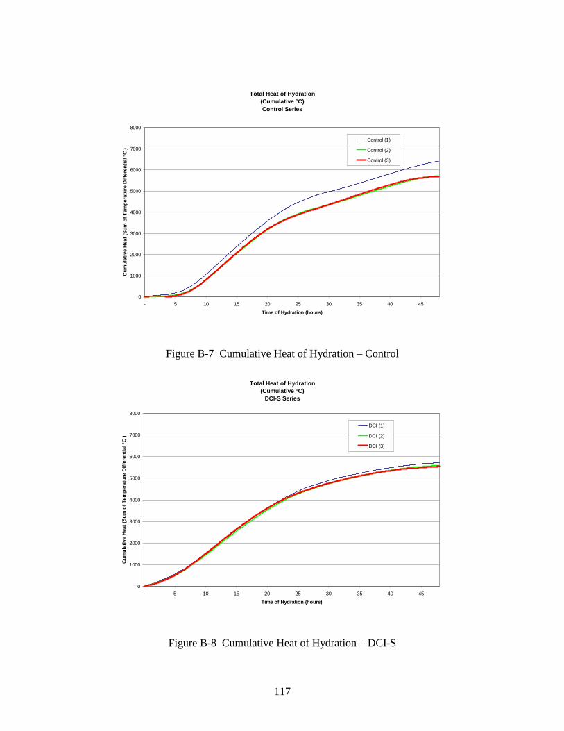
117

Total Heat of Hydration(Cumulative °C)Control Series

0

1000

2000

3000

4000

5000

6000

7000

8000

- 5 10 15 20 25 30 35 40 45Time of Hydration (hours)

Cum

ulat

ive

Hea

t (Su

m o

f Tem

pera

ture

Diff

eren

tial °

C )

Control (1)

Control (2)

Control (3)

Figure B-7 Cumulative Heat of Hydration – Control

Total Heat of Hydration(Cumulative °C)

DCI-S Series

0

1000

2000

3000

4000

5000

6000

7000

8000

- 5 10 15 20 25 30 35 40 45Time of Hydration (hours)

Cum

ulat

ive

Hea

t (Su

m o

f Tem

pera

ture

Diff

eren

tial °

C )

DCI (1)

DCI (2)

DCI (3)

Figure B-8 Cumulative Heat of Hydration – DCI-S

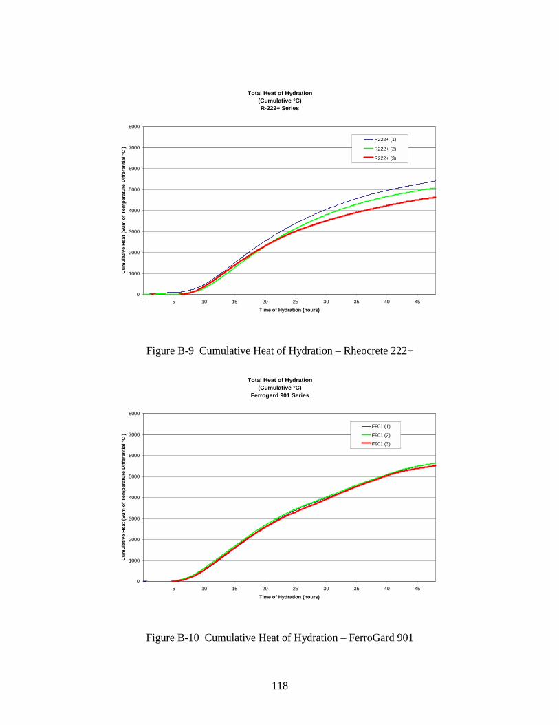
118

Total Heat of Hydration(Cumulative °C)R-222+ Series

0

1000

2000

3000

4000

5000

6000

7000

8000

- 5 10 15 20 25 30 35 40 45Time of Hydration (hours)

Cum

ulat

ive

Hea

t (Su

m o

f Tem

pera

ture

Diff

eren

tial °

C )

R222+ (1)

R222+ (2)

R222+ (3)

Figure B-9 Cumulative Heat of Hydration – Rheocrete 222+

Total Heat of Hydration(Cumulative °C)

Ferrogard 901 Series

0

1000

2000

3000

4000

5000

6000

7000

8000

- 5 10 15 20 25 30 35 40 45Time of Hydration (hours)

Cum

ulat

ive

Hea

t (Su

m o

f Tem

pera

ture

Diff

eren

tial °

C )

F901 (1)

F901 (2)

F901 (3)

Figure B-10 Cumulative Heat of Hydration – FerroGard 901

119

Total Heat of Hydration(Cumulative °C)MCI-2005 Series

0

1000

2000

3000

4000

5000

6000

7000

8000

- 5 10 15 20 25 30 35 40 45Time of Hydration (hours)

Cum

ulat

ive

Hea

t (Su

m o

f Tem

pera

ture

Diff

eren

tial °

C )

MCI-2005 (1)MCI-2005 (2)MCI-2005 (3)

Figure B-11 Cumulative Heat of Hydration – Catexol 1000

Total Heat of Hydration(Cumulative °C)

Catexol 1000 Series

0

1000

2000

3000

4000

5000

6000

7000

8000

- 5 10 15 20 25 30 35 40 45Time of Hydration (hours)

Cum

ulat

ive

Hea

t (Su

m o

f Tem

pera

ture

Diff

eren

tial °

C )

C1000 (1)

C1000 (2)

C1000 (3)

Figure B-12 Cumulative Heat of Hydration – MCI 2005

120

C - CHLORIDE PENETRABILITY BY ELECTRICAL CONDUCTANCE

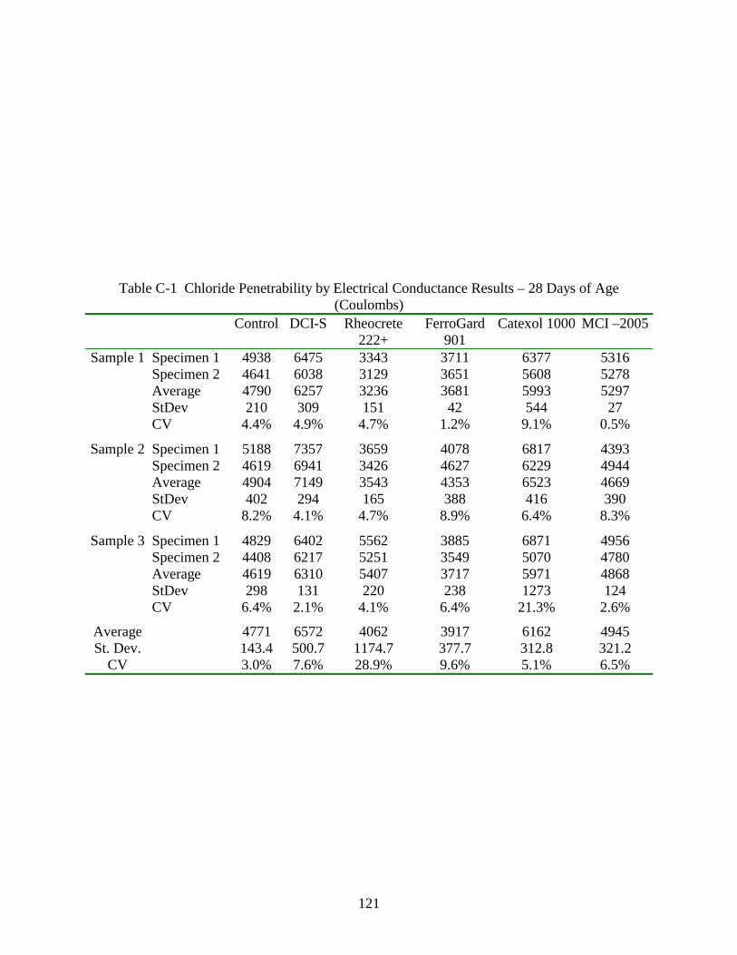
121

Table C-1 Chloride Penetrability by Electrical Conductance Results – 28 Days of Age (Coulombs)

Control DCI-S Rheocrete 222+

FerroGard 901

Catexol 1000 MCI –2005

Sample 1 Specimen 1 4938 6475 3343 3711 6377 5316 Specimen 2 4641 6038 3129 3651 5608 5278 Average 4790 6257 3236 3681 5993 5297 StDev 210 309 151 42 544 27 CV 4.4% 4.9% 4.7% 1.2% 9.1% 0.5%

Sample 2 Specimen 1 5188 7357 3659 4078 6817 4393 Specimen 2 4619 6941 3426 4627 6229 4944 Average 4904 7149 3543 4353 6523 4669 StDev 402 294 165 388 416 390 CV 8.2% 4.1% 4.7% 8.9% 6.4% 8.3%

Sample 3 Specimen 1 4829 6402 5562 3885 6871 4956 Specimen 2 4408 6217 5251 3549 5070 4780 Average 4619 6310 5407 3717 5971 4868 StDev 298 131 220 238 1273 124 CV 6.4% 2.1% 4.1% 6.4% 21.3% 2.6%

Average 4771 6572 4062 3917 6162 4945 St. Dev. 143.4 500.7 1174.7 377.7 312.8 321.2

CV 3.0% 7.6% 28.9% 9.6% 5.1% 6.5%

122

Table C-2 Chloride Penetrability by Electrical Conductance Results – 365 Days of Age (Coulombs)

Control DCI-S Rheocrete 222+

FerroGard 901

Catexol 1000 MCI –2005

Sample 1 Specimen 1 2794 3805 2064 2311 3863 3356 Specimen 2 2740 3636 2231 2464 4120 3097 Average 2767 3721 2148 2388 3992 3227 StDev 38 120 118 108 182 183 CV 1.4% 3.2% 5.5% 4.5% 4.6% 5.7%

Sample 2 Specimen 1 3109 4372 1939 2426 4279 2844 Specimen 2 2672 3982 1980 2463 4483 3519 Average 2891 4177 1960 2445 4381 3182 StDev 309 276 29 26 144 477 CV 10.7% 6.6% 1.5% 1.1% 3.3% 15.0%

Sample 3 Specimen 1 2920 3979 2063 2395 3501 2979 Specimen 2 2393 3813 2106 2420 3259 2857

Average 2657 3896 2085 2408 3380 2918 StDev 373 117 30 18 171 86 CV 14.0% 3.0% 1.5% 0.7% 5.1% 3.0%

Average 2771 3931 2064 2413 3918 3109 St. Dev. 117.1 230.3 95.7 28.9 504.6 166.6 CV 4.2% 5.9% 4.6% 1.2% 12.9% 5.4%

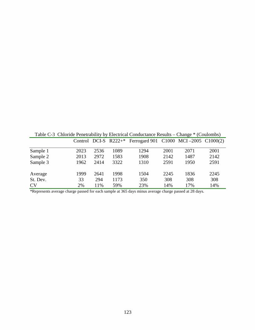
123

Table C-3 Chloride Penetrability by Electrical Conductance Results – Change * (Coulombs) Control DCI-S R222+* Ferrogard 901 C1000 MCI –2005 C1000(2)

Sample 1 2023 2536 1089 1294 2001 2071 2001 Sample 2 2013 2972 1583 1908 2142 1487 2142 Sample 3

1962 2414 3322 1310 2591 1950 2591

Average 1999 2641 1998 1504 2245 1836 2245 St. Dev. 33 294 1173 350 308 308 308 CV 2% 11% 59% 23% 14% 17% 14% *Represents average charge passed for each sample at 365 days minus average charge passed at 28 days.

124

DCI-SPermeability vs Time

0

1000

2000

3000

4000

5000

6000

7000

8000

0 100 200 300 400Age (days)

Perm

eabi

lity

(Cou

lom

bs)

ControlDCI-S

Figure C-1 Chloride Penetrability by Electrical Conductance – DCI-S vs. Control

Rheocrete 222+Permeability vs Time

0

1000

2000

3000

4000

5000

6000

7000

8000

0 100 200 300 400Age (days)

Perm

eabi

lity

(Cou

lom

bs)

ControlR222+*

Figure C-2 Chloride Penetrability by Electrical Conductance – Rheocrete 222+ vs. Control

125

FerroGard 901Permeability vs Time

0

1000

2000

3000

4000

5000

6000

7000

8000

0 100 200 300 400Age (days)

Perm

eabi

lity

(Cou

lom

bs)

ControlFerrogard 901

Figure C-3 Chloride Penetrability by Electrical Conductance – FerroGard 901 vs. Control

Catexol 1000Permeability vs Time

0

1000

2000

3000

4000

5000

6000

7000

8000

0 100 200 300 400Age (days)

Perm

eabi

lity

(Cou

lom

bs)

ControlC1000

Figure C-4 Chloride Penetrability by Electrical Conductance – Catexol 1000 vs. Control

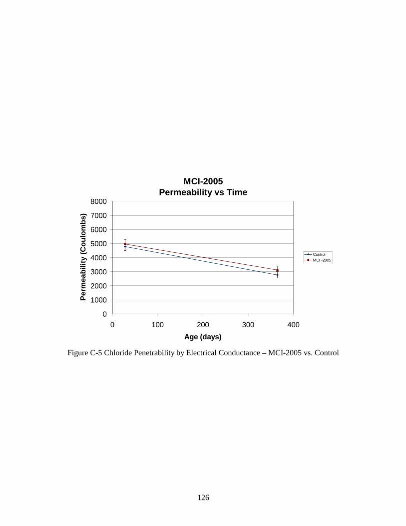
126

MCI-2005Permeability vs Time

0

1000

2000

3000

4000

5000

6000

7000

8000

0 100 200 300 400Age (days)

Perm

eabi

lity

(Cou

lom

bs)

ControlMCI -2005

Figure C-5 Chloride Penetrability by Electrical Conductance – MCI-2005 vs. Control

127

D - CHLORIDE PROFILES

128

Control DCI-S Rheocrete 222+

Figure D-1 Chloride Profiles after Two Years Ponding (Control, DCI-S, and Rheocrete 222+)

Chloride Profile0.0

10.020.030.040.050.060.070.0

0.0 2.0 4.0 6.0 8.0 10.0

Cl- Content (kg Cl-/m3 concrete)

Dep

th (m

m)

Control (1)

Chloride Profile0.0

10.020.030.040.050.060.070.0

0.0 2.0 4.0 6.0 8.0 10.0

Cl- Content (kg Cl-/m3 concrete)

Dep

th (m

m)

Control (3)

Chloride Profile0.0

10.020.030.040.050.060.070.0

0.0 2.0 4.0 6.0 8.0 10.0

Cl- Content (kg Cl-/m3 concrete)

Dep

th (m

m)

Rheocrete 222+ (1)

Chloride Profile0.0

10.020.030.040.050.060.070.0

0.0 2.0 4.0 6.0 8.0 10.0

Cl- Content (kg Cl-/m3 concrete)

Dep

th (m

m)

Rheocrete 222+ (2)

Chloride Profile0.0

10.020.030.040.050.060.070.0

0.0 2.0 4.0 6.0 8.0 10.0

Cl- Content (kg Cl-/m3 concrete)

Dep

th (m

m)

Rheocrete 222+ (3)

Chloride Profile0.0

10.020.030.040.050.060.070.0

0.0 2.0 4.0 6.0 8.0 10.0

Cl- Content (kg Cl-/m3 concrete)

Dep

th (m

m)

Control (2)

Chloride Profile0.0

10.020.030.040.050.060.070.0

0.0 2.0 4.0 6.0 8.0 10.0

Cl- Content (kg Cl-/m3 concrete)

Dep

th (m

m)

DCI-S (1)

Chloride Profile0.0

10.020.030.040.050.060.070.0

0.0 2.0 4.0 6.0 8.0 10.0

Cl- Content (kg Cl-/m3 concrete)

Dep

th (m

m)

DCI-S (2)

Chloride Profile0.0

10.020.030.040.050.060.070.0

0.0 2.0 4.0 6.0 8.0 10.0

Cl- Content (kg Cl-/m3 concrete)

Dep

th (m

m)

DCI-S (3)

129

FerroGard 901 Catexol 1000 MCI-2005

Figure D-2 Chloride Profiles after Two Years Ponding (FerroGard 901, Catexol 1000, and MCI-2005)

Chloride Profile0.0

10.020.030.040.050.060.070.0

0.0 2.0 4.0 6.0 8.0 10.0

Cl- Content (kg Cl-/m3 concrete)

Dep

th (m

m)

FerroGard 901 (1)

Chloride Profile0.0

10.020.030.040.050.060.070.0

0.0 2.0 4.0 6.0 8.0 10.0

Cl- Content (kg Cl-/m3 concrete)

Dep

th (m

m)

FerroGard 901 (2)

Chloride Profile0.0

10.020.030.040.050.060.070.0

0.0 2.0 4.0 6.0 8.0 10.0

Cl- Content (kg Cl-/m3 concrete)

Dep

th (m

m)

FerroGard 901 (3)

Chloride Profile0.0

10.020.030.040.050.060.070.0

0.0 2.0 4.0 6.0 8.0 10.0

Cl- Content (kg Cl-/m3 concrete)

Dep

th (m

m)

Catexol 1000 (1)

Chloride Profile0.0

10.020.030.040.050.060.070.0

0.0 2.0 4.0 6.0 8.0 10.0

Cl- Content (kg Cl-/m3 concrete)

Dep

th (m

m)

Catexol 1000 (2)

Chloride Profile0.0

10.020.030.040.050.060.070.0

0.0 2.0 4.0 6.0 8.0 10.0

Cl- Content (kg Cl-/m3 concrete)

Dep

th (m

m)

Catexol 1000 (3)

Chloride Profile0.0

10.020.030.040.050.060.070.0

0.0 2.0 4.0 6.0 8.0 10.0

Cl- Content (kg Cl-/m3 concrete)

Dep

th (m

m)

MCI-2005 (1)

Chloride Profile0.0

10.020.030.040.050.060.070.0

0.0 2.0 4.0 6.0 8.0 10.0

Cl- Content (kg Cl-/m3 concrete)

Dep

th (m

m)

MCI-2005 (2)

Chloride Profile0.0

10.020.030.040.050.060.070.0

0.0 2.0 4.0 6.0 8.0 10.0

Cl- Content (kg Cl-/m3 concrete)

Dep

th (m

m)

MCI-2005 (3)

130

E - CONCRETE ELECTROCHEMICAL TESTS

131

Figure E-1 Macro-Cell Corrosion – Control

MCB-C (Control)

0

10

20

30

40

50

60

70

80

90

100

110

120

130

140

150

2 4 6 8 10 12 14 16 18 20 22 24 26

Specimen Age (months)

Mac

ro C

urre

nt (

µ µµµA)

MCB-C-1a MCB-C-1b

Threshold

Macro Corrosion Current over Time

Begin ponding after initial tests

MCB-C (Control)

0

10

20

30

40

50

60

70

80

90

100

110

120

130

140

150

2 4 6 8 10 12 14 16 18 20 22 24 26

Specimen Age (months)

Mac

ro C

urre

nt (

µ µµµA)

MCB-C-2a MCB-C-2b

Threshold

Begin ponding after initial tests

Macro Corrosion Current over Time

MCB-C (Control)

0

10

20

30

40

50

60

70

80

90

100

110

120

130

140

150

2 4 6 8 10 12 14 16 18 20 22 24 26

Specimen Age (months)

Mac

ro C

urre

nt (

µ µµµA)

MCB-C-3a MCB-C-3b

Threshold

Begin ponding after initial tests

Macro Corrosion Current over Time

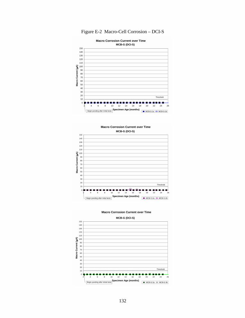
132

Figure E-2 Macro-Cell Corrosion – DCI-S

MCB-G (DCI-S)

0

10

20

30

40

50

60

70

80

90

100

110

120

130

140

150

2 4 6 8 10 12 14 16 18 20 22 24 26

Specimen Age (months)

Mac

ro C

urre

nt (

µ µµµA)

MCB-G-1a MCB-G-1b

Macro Corrosion Current over Time

Threshold

Begin ponding after initial tests

MCB-G (DCI-S)

0

10

20

30

40

50

60

70

80

90

100

110

120

130

140

150

2 4 6 8 10 12 14 16 18 20 22 24 26

Specimen Age (months)

Mac

ro C

urre

nt ( µ µµµ

A)

MCB-G-2a MCB-G-2b

Macro Corrosion Current over Time

Threshold

Begin ponding after initial tests

MCB-G (DCI-S)

0

10

20

30

40

50

60

70

80

90

100

110

120

130

140

150

2 4 6 8 10 12 14 16 18 20 22 24 26

Specimen Age (months)

Mac

ro C

urre

nt (

µ µµµA)

MCB-G-3a MCB-G-3b

Macro Corrosion Current over Time

Threshold

Begin ponding after initial tests

133

Figure E-3 Macro-Cell Corrosion – Rheocrete 222+

MCB-M (Rheocrete 222+)

0102030405060708090

100110120130140150

2 4 6 8 10 12 14 16 18 20 22 24 26

Specimen Age (months)

Mac

ro C

urre

nt (

µ µµµA)

MCB-M-1a MCB-M-1b

Macro Corrosion Current over Time

Begin ponding after initial tests

Threshold

MCB-M (Rheocrete 222+)

0

10

20

30

40

50

60

70

80

90

100

110

120

130

140

150

2 4 6 8 10 12 14 16 18 20 22 24 26

Specimen Age (months)

Mac

ro C

urre

nt (

µ µµµA)

MCB-M-2a MCB-M-2b

Macro Corrosion Current over Time

Begin ponding after initial tests

Threshold

MCB-M (Rheocrete 222+)

0

10

20

30

40

50

60

70

80

90

100

110

120

130

140

150

2 4 6 8 10 12 14 16 18 20 22 24 26

Specimen Age (months)

Mac

ro C

urre

nt (

µ µµµA)

MCB-M-3a MCB-M-3b

Macro Corrosion Current over Time

Begin ponding after initial

Threshold

134

Figure E-4 Macro-Cell Corrosion – FerroGard 901

MCB-X (Catexol 1000)

0102030405060708090

100110120130140150

2 4 6 8 10 12 14 16 18 20 22 24 26

Specimen Age (months)

Mac

ro C

urre

nt (

µ µµµA)

MCB-X-1a MCB-X-1b

Macro Corrosion Current over Time

Threshold

Begin ponding after initial

MCB-X (Catexol 1000)

0

10

20

30

40

50

60

70

80

90

100

110

120

130

140

150

2 4 6 8 10 12 14 16 18 20 22 24 26

Specimen Age (months)

Mac

ro C

urre

nt (

µ µµµA)

MCB-X-2a MCB-X-2b

Macro Corrosion Current over Time

Threshold

Begin ponding after initial

MCB-X (Catexol 1000)

0

10

20

30

40

50

60

70

80

90

100

110

120

130

140

150

2 4 6 8 10 12 14 16 18 20 22 24 26

Specimen Age (months)

Mac

ro C

urre

nt (

µ µµµA)

MCB-X-3a MCB-X-3b

Macro Corrosion Current over Time

Threshold

Begin ponding after initial

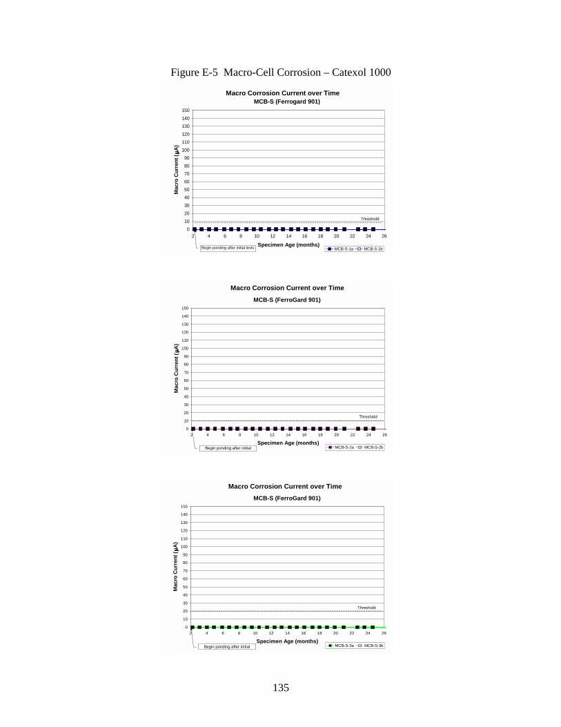
135

Figure E-5 Macro-Cell Corrosion – Catexol 1000

MCB-S (Ferrogard 901)

0102030405060708090

100110120130140150

2 4 6 8 10 12 14 16 18 20 22 24 26

Specimen Age (months)

Mac

ro C

urre

nt (

µ µµµA)

MCB-S-1a MCB-S-1b

Macro Corrosion Current over Time

Begin ponding after initial tests

Threshold

MCB-S (FerroGard 901)

0

10

20

30

40

50

60

70

80

90

100

110

120

130

140

150

2 4 6 8 10 12 14 16 18 20 22 24 26

Specimen Age (months)

Mac

ro C

urre

nt (

µ µµµA)

MCB-S-2a MCB-S-2b

Macro Corrosion Current over Time

Begin ponding after initial

Threshold

MCB-S (FerroGard 901)

0

10

20

30

40

50

60

70

80

90

100

110

120

130

140

150

2 4 6 8 10 12 14 16 18 20 22 24 26

Specimen Age (months)

Mac

ro C

urre

nt (

µ µµµA)

MCB-S-3a MCB-S-3b

Macro Corrosion Current over Time

Begin ponding after initial

Threshold

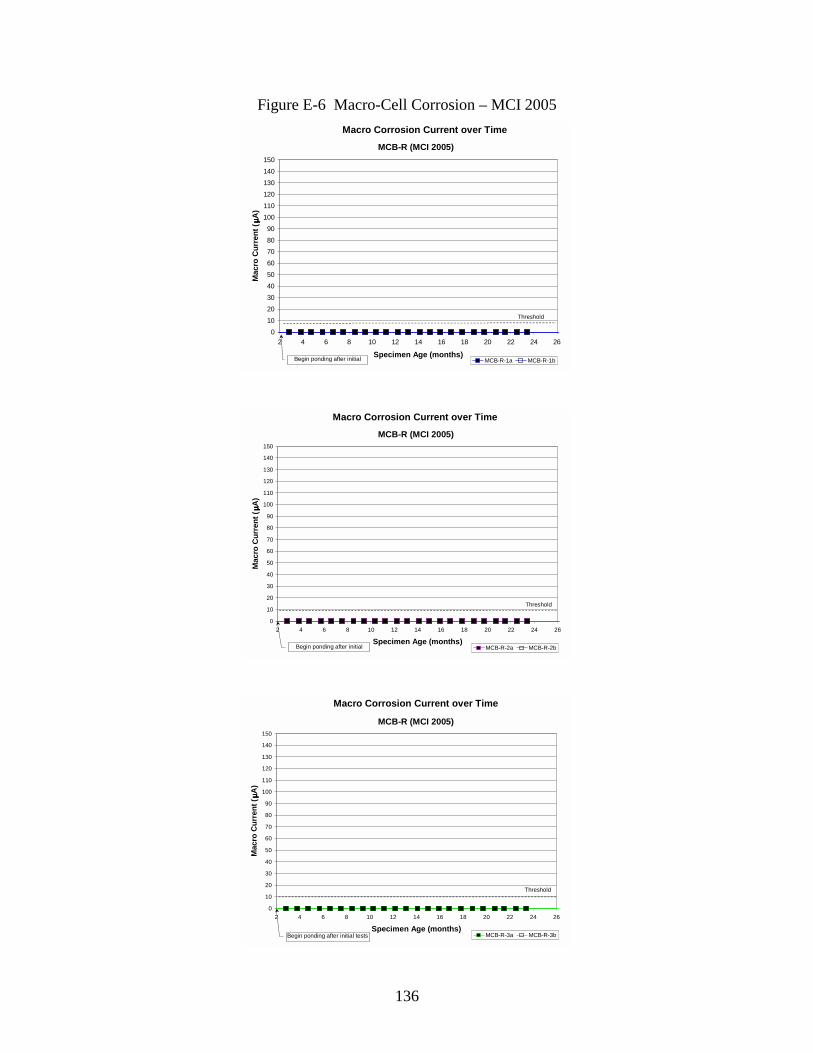
136

Figure E-6 Macro-Cell Corrosion – MCI 2005

MCB-R (MCI 2005)

0102030405060708090

100110120130140150

2 4 6 8 10 12 14 16 18 20 22 24 26

Specimen Age (months)

Mac

ro C

urre

nt (

µ µµµA)

MCB-R-1a MCB-R-1b

Macro Corrosion Current over Time

Threshold

Begin ponding after initial

MCB-R (MCI 2005)

0

10

20

30

40

50

60

70

80

90

100

110

120

130

140

150

2 4 6 8 10 12 14 16 18 20 22 24 26

Specimen Age (months)

Mac

ro C

urre

nt (

µ µµµA)

MCB-R-2a MCB-R-2b

Macro Corrosion Current over Time

Threshold

Begin ponding after initial

MCB-R (MCI 2005)

0

10

20

30

40

50

60

70

80

90

100

110

120

130

140

150

2 4 6 8 10 12 14 16 18 20 22 24 26

Specimen Age (months)

Mac

ro C

urre

nt (

µ µµµA)

MCB-R-3a MCB-R-3b

Macro Corrosion Current over Time

Threshold

Begin ponding after initial tests

137

Figure E-7 Electric Potential – Control

MCB-C (Control)

0

100

200

300

400

500

600

700

2 4 6 8 10 12 14 16 18 20 22 24 26

Specimen Age (months)

Ref

eren

ce P

oten

tial (

-mV

CSE

)

MCB-C-1a MCB-C-1b

High probability of corrosion

Begin ponding after initial tests

Reference Potential (CSE) Over

MCB-C (Control)

0

100

200

300

400

500

600

700

2 4 6 8 10 12 14 16 18 20 22 24 26

Specimen Age (months)

Ref

eren

ce P

oten

tial (

-mV

CSE

)

MCB-C-2a MCB-C-2b

High probability of Corrosion

Begin ponding after initial tests

Reference Potential (CSE) Over Time

MCB-C (Control)

0

100

200

300

400

500

600

700

2 4 6 8 10 12 14 16 18 20 22 24 26

Specimen Age (months)

Ref

eren

ce P

oten

tial (

-mV

CSE

)

MCB-C-3a MCB-C-3b

High probability of Corrosion

Begin ponding after initial tests

Reference Potential (CSE) Over Time

138

Figure E-8 Electric Potential – DCI-S

MCB-G (DCI-S)

0

100

200

300

400

500

600

700

2 4 6 8 10 12 14 16 18 20 22 24 26

Specimen Age (months)

Ref

eren

ce P

oten

tial (

-mV

CSE

)

MCB-G-1a MCB-G-1b

Reference Potential (CSE) Over Time

High probability of Corrosion

Begin ponding after initial tests

MCB-G (DCI-S)

0

100

200

300

400

500

600

700

2 4 6 8 10 12 14 16 18 20 22 24 26

Specimen Age (months)

Ref

eren

ce P

oten

tial (

-mV

CSE

)

MCB-G-2a MCB-G-2b

Reference Potential (CSE) Over Time

High probability of Corrosion

Begin ponding after initial tests

MCB-G (DCI-S)

0

100

200

300

400

500

600

700

2 4 6 8 10 12 14 16 18 20 22 24 26

Specimen Age (months)

Ref

eren

ce P

oten

tial (

-mV

CSE

)

MCB-G-3a MCB-G-3b

Reference Potential (CSE) Over Time

High probability of Corrosion

Begin ponding after initial tests

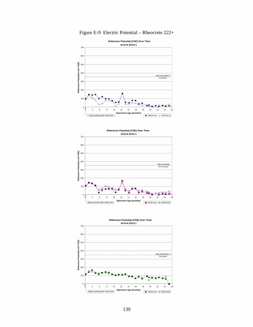
139

Figure E-9 Electric Potential – Rheocrete 222+

MCB-M (R222+)

0

100

200

300

400

500

600

700

2 4 6 8 10 12 14 16 18 20 22 24 26

Specimen Age (months)

Ref

eren

ce P

oten

tial (

-mV

CSE

)

MCB-M-1a MCB-M-1b

Reference Potential (CSE) Over Time

Begin ponding after initial tests

High probability of Corrosion

MCB-M (R222+)

0

100

200

300

400

500

600

700

2 4 6 8 10 12 14 16 18 20 22 24 26

Specimen Age (months)

Ref

eren

ce P

oten

tial (

-mV

CSE

)

MCB-M-2a MCB-M-2b

Reference Potential (CSE) Over Time

Begin ponding after initial tests

High probability of Corrosion

MCB-M (R222+)

0

100

200

300

400

500

600

700

2 4 6 8 10 12 14 16 18 20 22 24 26

Specimen Age (months)

Ref

eren

ce P

oten

tial (

-mV

CSE

)

MCB-M-3a MCB-M-3b

Reference Potential (CSE) Over Time

Begin ponding after initial tests

High probability of Corrosion

140

Figure E-10 Electric Potential – FerroGard 901

MCB-S (Ferrogard 901)

0

100

200

300

400

500

600

700

2 4 6 8 10 12 14 16 18 20 22 24 26

Specimen Age (months)

Ref

eren

ce P

oten

tial (

-mV

CSE

)

MCB-S-1a MCB-S-1b

Reference Potential (CSE) Over Time

High probability of Corrosion

Begin ponding after initial tests

MCB-S (Ferrogard 901)

0

100

200

300

400

500

600

700

2 4 6 8 10 12 14 16 18 20 22 24 26

Specimen Age (months)

Ref

eren

ce P

oten

tial (

-mV

CSE

)

MCB-S-2a MCB-S-2b

Reference Potential (CSE) Over Time

High probability of Corrosion

Begin ponding after initial tests

MCB-S (Ferrogard 901)

0

100

200

300

400

500

600

700

2 4 6 8 10 12 14 16 18 20 22 24 26

Specimen Age (months)

Ref

eren

ce P

oten

tial (

-mV

CSE

)

MCB-S-3a MCB-S-3b

Reference Potential (CSE) Over Time

High probability of Corrosion

Begin ponding after initial tests

141

Figure E-11 Electric Potential – Catexol 1000

MCB-X (Catexol 1000)

0

100

200

300

400

500

600

700

2 4 6 8 10 12 14 16 18 20 22 24 26

Specimen Age (months)

Ref

eren

ce P

oten

tial (

-mV

CSE

)

MCB-X-1a MCB-X-1b

Reference Potential (CSE) Over Time

High probability of Corrosion

Begin ponding after initial tests

MCB-X (Catexol 1000)

0

100

200

300

400

500

600

700

2 4 6 8 10 12 14 16 18 20 22 24 26

Specimen Age (months)

Ref

eren

ce P

oten

tial (

-mV

CSE

)

MCB-X-2a MCB-X-2b

Reference Potential (CSE) Over Time

High probability of Corrosion

Begin ponding after initial

MCB-X (Catexol 1000)

0

100

200

300

400

500

600

700

2 4 6 8 10 12 14 16 18 20 22 24 26

Specimen Age (months)

Ref

eren

ce P

oten

tial (

-mV

CSE

)

MCB-X-3a MCB-X-3b

Reference Potential (CSE) Over Time

High probability of Corrosion

Begin ponding after initial tests

142

Figure E-12 Electric Potential – MCI 2005

MCB-R (MCI 2005)

0

100

200

300

400

500

600

700

2 4 6 8 10 12 14 16 18 20 22 24 26

Specimen Age (months)

Ref

eren

ce P

oten

tial (

-mV

CSE

)

MCB-R-1a MCB-R-1b

Reference Potential (CSE) Over Time

High probability of Corrosion

Begin ponding after initial tests

MCB-R (MCI 2005)

0

100

200

300

400

500

600

700

2 4 6 8 10 12 14 16 18 20 22 24 26

Specimen Age (months)

Ref

eren

ce P

oten

tial (

-mV

CSE

)

MCB-R-2a MCB-R-2b

Reference Potential (CSE) Over Time

High probability of Corrosion

Begin ponding after initial

MCB-R (MCI 2005)

0

100

200

300

400

500

600

700

2 4 6 8 10 12 14 16 18 20 22 24 26

Specimen Age (months)

Ref

eren

ce P

oten

tial (

-mV

CSE

)

MCB-R-3a MCB-R-3b

Reference Potential (CSE) Over Time

High probability of Corrosion

Begin ponding after initial

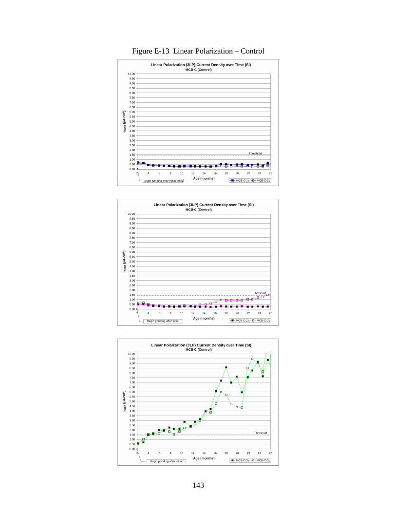
143

Figure E-13 Linear Polarization – Control

MCB-C (Control)

0.000.501.001.502.002.503.003.504.004.505.005.506.006.507.007.508.008.509.009.50

10.00

2 4 6 8 10 12 14 16 18 20 22 24 26

Age (months)

i CO

RR

( µA

/cm

2 )

MCB-C-1a MCB-C-1bBegin ponding after initial tests

Threshold

Linear Polarization (3LP) Current Density over Time (SI)

MCB-C (Control)

0.000.501.001.502.002.503.003.504.004.505.005.506.006.507.007.508.008.509.009.50

10.00

2 4 6 8 10 12 14 16 18 20 22 24 26

Age (months)

i CO

RR

( µA

/cm

2 )

MCB-C-2a MCB-C-2bBegin ponding after initial

Threshold

Linear Polarization (3LP) Current Density over Time (SI)

MCB-C (Control)

0.000.501.001.502.002.503.003.504.004.505.005.506.006.507.007.508.008.509.009.50

10.00

2 4 6 8 10 12 14 16 18 20 22 24 26

Age (months)

i CO

RR

( µA

/cm

2 )

MCB-C-3a MCB-C-3bBegin ponding after initial

Threshold

Linear Polarization (3LP) Current Density over Time (SI)

144

Figure E-14 Linear Polarization – DCI-S

MCB-G (DCI-S)

0.000.501.001.502.002.503.003.504.004.505.005.506.006.507.007.508.008.509.009.50

10.00

2 4 6 8 10 12 14 16 18 20 22 24 26

Age (months)

i CO

RR

( µA

/cm

2 )

MCB-G-1a MCB-G-1bBegin ponding after initial tests

Threshold

Linear Polarization (3LP) Corrosion Current Density over Time (SI)

MCB-G (DCI-S)

0.000.501.001.502.002.503.003.504.004.505.005.506.006.507.007.508.008.509.009.50

10.00

2 4 6 8 10 12 14 16 18 20 22 24 26

Age (months)

i CO

RR

( µA

/cm

2 )

MCB-G-2a MCB-G-2bBegin ponding after initial

Threshold

Linear Polarization (3LP) Corrosion Current Density over Time (SI)

MCB-G (DCI-S)

0.000.501.001.502.002.503.003.504.004.505.005.506.006.507.007.508.008.509.009.50

10.00

2 4 6 8 10 12 14 16 18 20 22 24 26

Age (months)

i CO

RR

( µA

/cm

2 )

MCB-G-3a MCB-G-3bBegin ponding after initial tests

Threshold

Linear Polarization (3LP) Corrosion Current Density over Time (SI)

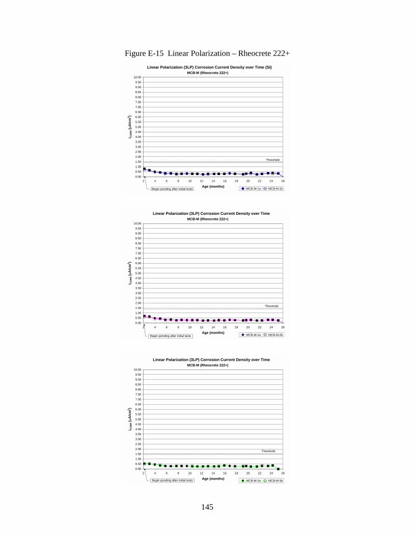
145

Figure E-15 Linear Polarization – Rheocrete 222+

MCB-M (Rheocrete 222+)

0.000.501.001.502.002.503.003.504.004.505.005.506.006.507.007.508.008.509.009.50

10.00

2 4 6 8 10 12 14 16 18 20 22 24 26

Age (months)

i CO

RR

( µA

/cm

2 )

MCB-M-1a MCB-M-1b

Linear Polarization (3LP) Corrosion Current Density over Time (SI)

Threshold

Begin ponding after initial tests

MCB-M (Rheocrete 222+)

0.000.501.001.502.002.503.003.504.004.505.005.506.006.507.007.508.008.509.009.50

10.00

2 4 6 8 10 12 14 16 18 20 22 24 26

Age (months)

i CO

RR

( µA

/cm

2 )

MCB-M-2a MCB-M-2b

Linear Polarization (3LP) Corrosion Current Density over Time

Threshold

Begin ponding after initial tests

MCB-M (Rheocrete 222+)

0.000.501.001.502.002.503.003.504.004.505.005.506.006.507.007.508.008.509.009.50

10.00

2 4 6 8 10 12 14 16 18 20 22 24 26

Age (months)

i CO

RR

( µA

/cm

2 )

MCB-M-3a MCB-M-3b

Linear Polarization (3LP) Corrosion Current Density over Time

Threshold

Begin ponding after initial tests

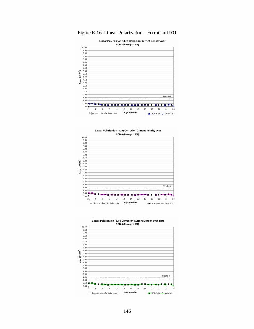
146

Figure E-16 Linear Polarization – FerroGard 901

MCB-S (Ferrogard 901)

0.000.501.001.502.002.503.003.504.004.505.005.506.006.507.007.508.008.509.009.50

10.00

2 4 6 8 10 12 14 16 18 20 22 24 26

Age (months)

i CO

RR

( µA

/cm

2 )

MCB-S-1a MCB-S-1b

Linear Polarization (3LP) Corrosion Current Density over

Begin ponding after initial tests

Threshold

MCB-S (Ferrogard 901)

0.000.501.001.502.002.503.003.504.004.505.005.506.006.507.007.508.008.509.009.50

10.00

2 4 6 8 10 12 14 16 18 20 22 24 26

Age (months)

i CO

RR

( µA

/cm

2 )

MCB-S-2a MCB-S-2b

Linear Polarization (3LP) Corrosion Current Density over

Begin ponding after initial tests

Threshold

MCB-S (Ferrogard 901)

0.000.501.001.502.002.503.003.504.004.505.005.506.006.507.007.508.008.509.009.50

10.00

2 4 6 8 10 12 14 16 18 20 22 24 26

Age (months)

i CO

RR

( µA

/cm

2 )

MCB-S-3a MCB-S-3b

Linear Polarization (3LP) Corrosion Current Density over Time

Begin ponding after initial tests

Threshold

147

Figure E-17 Linear Polarization – Catexol 1000

MCB-X (Catexol 1000)

0.000.501.001.502.002.503.003.504.004.505.005.506.006.507.007.508.008.509.009.50

10.00

2 4 6 8 10 12 14 16 18 20 22 24 26

Age (months)

i CO

RR

( µA

/cm

2 )

MCB-X-1a MCB-X-1b

Linear Polarization (3LP) Corrosion Current Density over Time (SI)

Begin ponding after initial t t

Threshold

MCB-X (Catexol 1000)

0.000.501.001.502.002.503.003.504.004.505.005.506.006.507.007.508.008.509.009.50

10.00

2 4 6 8 10 12 14 16 18 20 22 24 26

Age (months)

iCO

RR (

µA/c

m2 )

MCB-X-3a MCB-X-3b

Linear Polarization (3LP) Corrosion Current Density over Time (SI)

Begin ponding after initial tests

Threshold

MCB-X (Catexol 1000)

0.000.501.001.502.002.503.003.504.004.505.005.506.006.507.007.508.008.509.009.50

10.00

2 4 6 8 10 12 14 16 18 20 22 24 26

Age (months)

iCO

RR (

µA/c

m2 )

MCB-X-2a MCB-X-2b

Linear Polarization (3LP) Corrosion Current Density over Time (SI)

Begin ponding after initial tests

Threshold

148

Figure E-18 Linear Polarization – MCI 2005

MCB-R (MCI 2005)

0.000.501.001.502.002.503.003.504.004.505.005.506.006.507.007.508.008.509.009.50

10.00

2 4 6 8 10 12 14 16 18 20 22 24 26

Age (months)

iCO

RR (

µA/c

m2 )

MCB-R-1a MCB-R-1b

Linear Polarization (3LP) Corrosion Current Density over Time (SI)

Begin ponding after initial tests

Threshold

MCB-R (MCI 2005)

0.000.501.001.502.002.503.003.504.004.505.005.506.006.507.007.508.008.509.009.50

10.00

2 4 6 8 10 12 14 16 18 20 22 24 26

Age (months)

iCO

RR (

µA/c

m2 )

MCB-R-2a MCB-R-2b

Linear Polarization (3LP) Corrosion Current Density over Time (SI)

Begin ponding after initial tests

Threshold

MCB-R (MCI 2005)

0.000.501.001.502.002.503.003.504.004.505.005.506.006.507.007.508.008.509.009.50

10.00

2 4 6 8 10 12 14 16 18 20 22 24 26

Age (months)

iCO

RR (

µA/c

m2 )

MCB-R-3a MCB-R-3b

Linear Polarization (3LP) Corrosion Current Density over Time (SI)

Begin ponding after initial tests

Threshold

149

Figure E-19 Temperature – Control and DCI-S

Temperature Trends

0

5

10

15

20

25

30

0 2 4 6 8 10 12 14 16 18 20 22 24

Specimen Age (days)

Inte

rnal

Tem

pera

ture

(°C

)

Control (1)Control (2)Control (3)Lab

Control

Spring Summer Fall Winter Spring Summer Fall Winter Spring

Temperature Trends

0

5

10

15

20

25

30

0 2 4 6 8 10 12 14 16 18 20 22 24

Specimen Age (days)

Inte

rnal

Tem

pera

ture

(°C

)

DCI-S (1)DCI-S (2)DCI-S (3)Lab

DCI-S

Spring Summer Fall Winter Spring Summer Fall Winter Spring

150

Figure E-20 Temperature – Rheocrete 222+ and FerroGard 901

Temperature Trends

0

5

10

15

20

25

30

0 2 4 6 8 10 12 14 16 18 20 22 24

Specimen Age (days)

Inte

rnal

Tem

pera

ture

(°C

)

Rheocrete 222+ (1)Rheocrete 222+ (2)Rheocrete 222+ (3)Lab

Rheocrete 222+

Spring Summer Fall Winter Spring Summer Fall Winter Spring

Temperature Trends

0

5

10

15

20

25

30

0 2 4 6 8 10 12 14 16 18 20 22 24

Specimen Age (days)

Inte

rnal

Tem

pera

ture

(°C

)

FerroGard 901 (1)FerroGard 901 (2)FerroGard 901 (3)Lab

FerroGard 901

Spring Summer Fall Winter Spring Summer Fall Winter Spring

151

Figure E-21 Temperature – Catexol 1000 and MCI 2005

Temperature Trends

0

5

10

15

20

25

30

0 2 4 6 8 10 12 14 16 18 20 22 24

Specimen Age (days)

Inte

rnal

Tem

pera

ture

(°C

)

Catexol 1000 (1)Catexol 1000 (2)Catexol 1000 (3)Lab

Catexol 1000

Spring Summer Fall Winter Spring Summer Fall Winter Spring

Temperature Trends

0

5

10

15

20

25

30

0 2 4 6 8 10 12 14 16 18 20 22 24

Specimen Age (days)

Inte

rnal

Tem

pera

ture

(°C

)

MCI-2005 (1)MCI-2005 (2)MCI-2005 (3)Lab

MCI-2005

Spring Summer Fall Winter Spring Summer Fall Winter Spring

152

Figure E-22 Relative Humidity – Control and DCI-S

Relative Humidity Trends

0%

20%

40%

60%

80%

100%

120%

140%

0 2 4 6 8 10 12 14 16 18 20 22 24

Specimen Age (days)

Inte

rnal

Rel

ativ

e H

umid

ty (%

)

Control (1)Control (2)Control (3)Lab

Control

Spring Summer Fall Winter Spring Summer Fall Winter Spring

Relative Humidity Trends

0%

20%

40%

60%

80%

100%

120%

140%

0 2 4 6 8 10 12 14 16 18 20 22 24

Specimen Age (days)

Inte

rnal

Rel

ativ

e H

umid

ty (%

)

DCI-S (1)DCI-S (2)DCI-S (3)Lab

DCI-S

Spring Summer Fall Winter Spring Summer Fall Winter Spring

153

Figure E-23 Relative Humidity – Rheocrete 222+ and FerroGard 901

Relative Humidity Trends

0%

20%

40%

60%

80%

100%

120%

140%

0 2 4 6 8 10 12 14 16 18 20 22 24

Specimen Age (days)

Inte

rnal

Rel

ativ

e H

umid

ty (%

)

Rheocrete 222+ (1)Rheocrete 222+ (2)Rheocrete 222+ (3)Lab

Rheocrete 222+

Spring Summer Fall Winter Spring Summer Fall Winter Spring

Relative Humidity Trends

0%

20%

40%

60%

80%

100%

120%

140%

0 2 4 6 8 10 12 14 16 18 20 22 24

Specimen Age (days)

Inte

rnal

Rel

ativ

e H

umid

ty (%

)

FerroGard 901 (1)FerroGard 901 (2)FerroGard 901 (3)Lab

FerroGard 901

Spring Summer Fall Winter Spring Summer Fall Winter Spring

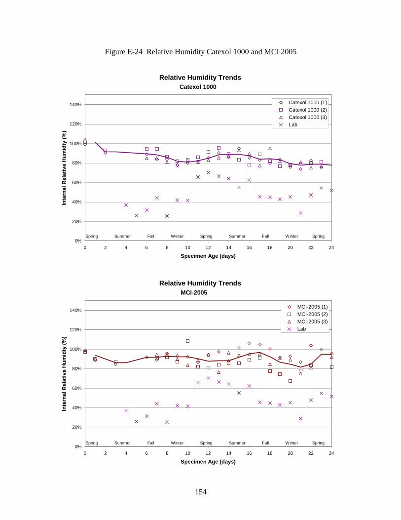
154

Figure E-24 Relative Humidity Catexol 1000 and MCI 2005

Relative Humidity Trends

0%

20%

40%

60%

80%

100%

120%

140%

0 2 4 6 8 10 12 14 16 18 20 22 24

Specimen Age (days)

Inte

rnal

Rel

ativ

e H

umid

ty (%

)

Catexol 1000 (1)Catexol 1000 (2)Catexol 1000 (3)Lab

Catexol 1000

Spring Summer Fall Winter Spring Summer Fall Winter Spring

Relative Humidity Trends

0%

20%

40%

60%

80%

100%

120%

140%

0 2 4 6 8 10 12 14 16 18 20 22 24

Specimen Age (days)

Inte

rnal

Rel

ativ

e H

umid

ty (%

)

MCI-2005 (1)MCI-2005 (2)MCI-2005 (3)Lab

MCI-2005

Spring Summer Fall Winter Spring Summer Fall Winter Spring

155

F - ELECTROCHEMICAL SOLUTION SCREENING TEST

156

Proposed ASTM Test Method for Corrosion Inhibiting Admixtures for Steel Reinforcement in Concrete GCP will provide the following items. • Type I/II cement (C3A content between 6 and 10%) (2kg) • Filter paper with 1.1µm retention (10) • Teflon stir bars (2) • C1215 corrosion test samples (8) The round robin will consist of 8 electrochemical measurements: 2 controls at 0.5 M NaCl, 2 controls at 1M NaCl, 2 at 0.5M NaCl with 35mL/L standard calcium nitrite solution and 2 at 1M NaCl with 35mL/L standard calcium nitrite solution. Solution Preparation • Mix 1000 grams of distilled water and 200 grams of cement. Add the corrosion inhibitor,

35mL of a 30% calcium nitrite solution (the dosage rate of 35 mL/L is equivalent to 5L/m3 in concrete). One liter of solution is required for a single test. Stir the mixture for 60 minutes. Make sure the cement is well mixed in the solution during the 60 minute stir.

• After stirring filtrate the solution using filter paper with a retention of 1.1 µm. • Add 4 g/L of calcium hydroxide to the filtered solution and stir for 30 minutes. Electrochemical measurements • Setup a standard electrochemical cell according to ASTM G 59. • Purge the cell with carbon dioxide free air. The flow rate should be at least

300cc/minute. • Prior to placing samples in the electrochemical cell, they should be properly degreased.

Ultrasonic treatment for 2 minutes in hexane works well. If you do not have an ultrasonic bath, soak the samples in hexane and wipe dry. Make sure the samples are dry before placing them in the electrochemical cell.

• While purging the cell with C02 free air precondition the electrode in the solution for 20 hours at open circuit.

Several methods can be used to obtain carbon dioxide free air: 1. Carbon dioxide free air can be generated by passing house air through a saturated calcium

hydroxide solution. Phenolphthalein is used to monitor the solution pH. The color changes from magenta to light pink when the pH decreases due to the formation of carbonate. When this happens the solution should be replaced.

2. Purchase CO2 free air gas cylinders 3. CO2 free air gas generator (typically used for FT-IR equipment). Method (1) is the simplest and least expensive way to generate carbon dioxide free air. The source of air should have less than l ppm CO2.

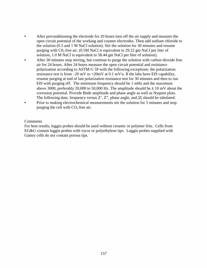
157

• After preconditioning the electrode for 20 hours turn off the air supply and measure the

open circuit potential of the working and counter electrodes. Then add sodium chloride to the solution (0.5 and 1 M NaCl solution). Stir the solution for 30 minutes and resume purging with C02 free air. (0.5M NaCl is equivalent to 29.22 gm NaCl per liter of solution, 1.0 M NaCl is equivalent to 58.44 gm NaCl per liter of solution).

• After 30 minutes stop stirring, but continue to purge the solution with carbon dioxide free air for 24 hours. After 24 hours measure the open circuit potential and resistance polarization according to ASTM G 59 with the following exceptions: the polarization resistance test is from –20 mV to +20mV at 0.1 mV/s. If the labs have EIS capability, resume purging at end of last polarization resistance test for 30 minutes and then to run EIS with purging off. The minimum frequency should be 1 mHz and the maximum above 3000, preferably 20,000 to 50,000 Hz. The amplitude should be ± 10 mV about the corrosion potential. Provide Bode amplitude and phase angle as well as Nyquist plots. The following data: frequency versus Z’, Z”, phase angle, and |Z| should be tabulated.

• Prior to making electrochemical measurements stir the solution for 5 minutes and stop purging the cell with CO2 free air.

Comments For best results, luggin probes should be used without ceramic or polymer frits. Cells from EG&G contain luggin probes with vycor or polyethylene tips. Luggin probes supplied with Gamry cells do not contain porous tips.

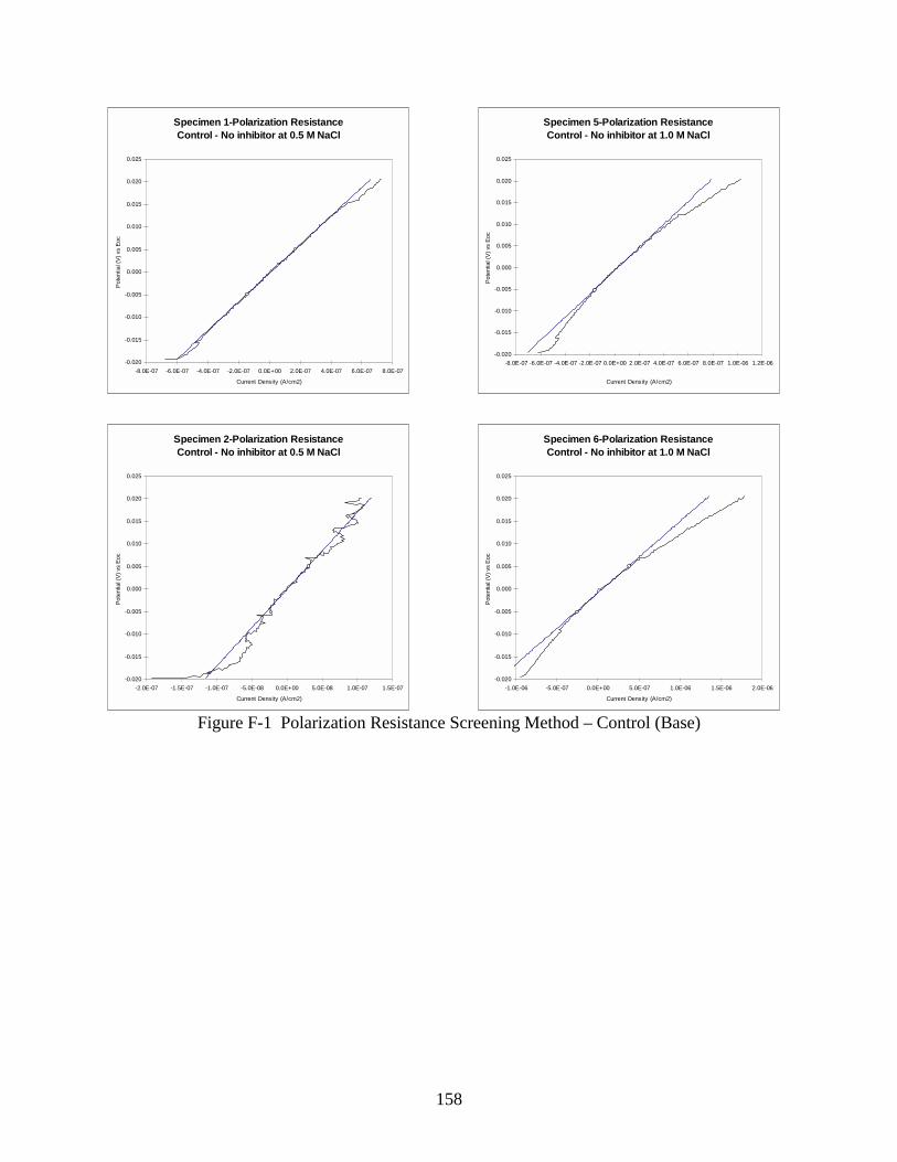
158

Figure F-1 Polarization Resistance Screening Method – Control (Base)

Specimen 1-Polarization ResistanceControl - No inhibitor at 0.5 M NaCl

-0.020

-0.015

-0.010

-0.005

0.000

0.005

0.010

0.015

0.020

0.025

-8.0E-07 -6.0E-07 -4.0E-07 -2.0E-07 0.0E+00 2.0E-07 4.0E-07 6.0E-07 8.0E-07

Current Density (A/cm2)

Pote

ntia

l (V)

vs

Eoc

Specimen 2-Polarization ResistanceControl - No inhibitor at 0.5 M NaCl

-0.020

-0.015

-0.010

-0.005

0.000

0.005

0.010

0.015

0.020

0.025

-2.0E-07 -1.5E-07 -1.0E-07 -5.0E-08 0.0E+00 5.0E-08 1.0E-07 1.5E-07

Current Density (A/cm2)

Pote

ntia

l (V)

vs

Eoc

Specimen 5-Polarization ResistanceControl - No inhibitor at 1.0 M NaCl

-0.020

-0.015

-0.010

-0.005

0.000

0.005

0.010

0.015

0.020

0.025

-8.0E-07 -6.0E-07 -4.0E-07 -2.0E-07 0.0E+00 2.0E-07 4.0E-07 6.0E-07 8.0E-07 1.0E-06 1.2E-06

Current Density (A/cm2)

Pote

ntia

l (V)

vs

Eoc

Specimen 6-Polarization ResistanceControl - No inhibitor at 1.0 M NaCl

-0.020

-0.015

-0.010

-0.005

0.000

0.005

0.010

0.015

0.020

0.025

-1.0E-06 -5.0E-07 0.0E+00 5.0E-07 1.0E-06 1.5E-06 2.0E-06

Current Density (A/cm2)

Pote

ntia

l (V)

vs

Eoc

159

Figure F-2 Polarization Resistance Screening Method – DCI (Base)

Specimen 3-Polarization Resistance35 mL DCI at 0.5 NaCl

-0.020

-0.015

-0.010

-0.005

0.000

0.005

0.010

0.015

0.020

0.025

-1.0E-07 -8.0E-08 -6.0E-08 -4.0E-08 -2.0E-08 0.0E+00 2.0E-08 4.0E-08

Current Density (A/cm2)

Pote

ntia

l (V)

vs

Eoc

Specimen 4-Polarization Resistance35 mL DCI at 0.5 M NaCl

-0.020

-0.015

-0.010

-0.005

0.000

0.005

0.010

0.015

0.020

-4.0E-08 -3.0E-08 -2.0E-08 -1.0E-08 0.0E+00 1.0E-08 2.0E-08 3.0E-08

Current Density (A/cm2)

Pote

ntia

l (V)

vs

Eoc

Specimen 7-Polarization Resistance35 mL DCI at 1.0 M NaCl

-0.025

-0.020

-0.015

-0.010

-0.005

0.000

0.005

0.010

0.015

0.020

-1.0E-07 -5.0E-08 0.0E+00 5.0E-08 1.0E-07 1.5E-07

Current Density (A/cm2)

Pote

ntia

l (V)

vs

Eoc

Specimen 8-Polarization Resistance35 mL DCI at 1.0 M NaCl

-0.020

-0.015

-0.010

-0.005

0.000

0.005

0.010

0.015

0.020

0.025

-4.0E-07 -3.0E-07 -2.0E-07 -1.0E-07 0.0E+00 1.0E-07 2.0E-07 3.0E-07

Current Density (A/cm2)

Pote

ntia

l (V)

vs

Eoc

160

Figure F-3 Polarization Resistance Screening Method – DCI (Extended)

Specimen 9-Polarization Resistance35 mL DCI at 2.0 M NaCl

-0.020

-0.015

-0.010

-0.005

0.000

0.005

0.010

0.015

0.020

0.025

-8.0E-07 -6.0E-07 -4.0E-07 -2.0E-07 0.0E+00 2.0E-07 4.0E-07

Current Density (A/cm2)

Pote

ntia

l (V)

vs

Eoc

Specimen 10-Polarization Resistance35 mL DCI at 2.0 M NaCl

-0.020

-0.015

-0.010

-0.005

0.000

0.005

0.010

0.015

0.020

0.025

-1.5E-06 -1.0E-06 -5.0E-07 0.0E+00 5.0E-07 1.0E-06 1.5E-06

Current Density (A/cm2)

Pote

ntia

l (V)

vs

Eoc

Specimen 11-Polarization Resistance35 mL DCI at 3.0 M NaCl

-0.020

-0.015

-0.010

-0.005

0.000

0.005

0.010

0.015

0.020

0.025

-1.0E-06 -8.0E-07 -6.0E-07 -4.0E-07 -2.0E-07 0.0E+00 2.0E-07 4.0E-07 6.0E-07

Current Density (A/cm2)

Pote

ntia

l (V)

vs

Eoc

Specimen 12-Polarization Resistance35 mL DCI at 3.0 M NaCl

-0.020

-0.015

-0.010

-0.005

0.000

0.005

0.010

0.015

0.020

0.025

-1.5E-06 -1.0E-06 -5.0E-07 0.0E+00 5.0E-07 1.0E-06

Current Density (A/cm2)

Pote

ntia

l (V)

vs

Eoc

161

Figure F-4 Polarization Resistance Screening Method – FerroGard 901 (Extended)

Specimen 13-Polarization Resistance35 mL Ferrogard 901 at 1.0 M NaCl

-0.020

-0.015

-0.010

-0.005

0.000

0.005

0.010

0.015

0.020

0.025

-6.0E-07 -4.0E-07 -2.0E-07 0.0E+00 2.0E-07 4.0E-07 6.0E-07

Current Density (A/cm2)

Pote

ntia

l (V)

vs

Eoc

Specimen 14-Polarization Resistance35 mL Ferrogard 901 at 1.0 M NaCl

-0.020

-0.015

-0.010

-0.005

0.000

0.005

0.010

0.015

0.020

0.025

-8.0E-07 -6.0E-07 -4.0E-07 -2.0E-07 0.0E+00 2.0E-07 4.0E-07 6.0E-07 8.0E-07 1.0E-06

Current Density (A/cm2)

Pote

ntia

l (V)

vs

Eoc

Specimen 19-Polarization Resistance35 mL Ferrogard 901 at 0.5 M NaCl

-0.020

-0.015

-0.010

-0.005

0.000

0.005

0.010

0.015

0.020

0.025

-4.0E-07 -3.0E-07 -2.0E-07 -1.0E-07 0.0E+00 1.0E-07 2.0E-07 3.0E-07

Current Density (A/cm2)

Pote

ntia

l (V)

vs

Eoc

Specimen 20-Polarization Resistance35 mL Ferrogard 901 at 0.5 M NaCl

-0.020

-0.015

-0.010

-0.005

0.000

0.005

0.010

0.015

0.020

0.025

-6.0E-07 -4.0E-07 -2.0E-07 0.0E+00 2.0E-07 4.0E-07 6.0E-07 8.0E-07

Current Density (A/cm2)

Pote

ntia

l (V)

vs

Eoc

162

Figure F-5 Polarization Resistance Screening Method – Rheocrete 222+ (Extended)

Specimen 15-Polarization Resistance35 mL Rheocrete 222+ at 0.5 M NaCl

-0.025

-0.020

-0.015

-0.010

-0.005

0.000

0.005

0.010

0.015

0.020

0.025

-8.0E-07 -6.0E-07 -4.0E-07 -2.0E-07 0.0E+00 2.0E-07 4.0E-07 6.0E-07 8.0E-07 1.0E-06

Current Density (A/cm2)

Pote

ntia

l (V)

vs

Eoc

Specimen 16-Polarization Resistance35 mL Rheocrete 222+ at 0.5 M NaCl

-0.025

-0.020

-0.015

-0.010

-0.005

0.000

0.005

0.010

0.015

0.020

0.025

-1.5E-06 -1.0E-06 -5.0E-07 0.0E+00 5.0E-07 1.0E-06 1.5E-06 2.0E-06

Current Density (A/cm2)

Pote

ntia

l (V)

vs

Eoc

Specimen 17-Polarization Resistance35 mL Rheocrete 222+ at 1.0 M NaCl

-0.020

-0.015

-0.010

-0.005

0.000

0.005

0.010

0.015

0.020

-1.0E-06 -5.0E-07 0.0E+00 5.0E-07 1.0E-06 1.5E-06

Current Density (A/cm2)

Pote

ntia

l (V)

vs

Eoc

Specimen 18-Polarization Resistance35 mL Rheocrete 222+ at 1.0 M NaCl

-0.020

-0.015

-0.010

-0.005

0.000

0.005

0.010

0.015

0.020

0.025

-6.0E-07 -4.0E-07 -2.0E-07 0.0E+00 2.0E-07 4.0E-07 6.0E-07

Current Density (A/cm2)

Pote

ntia

l (V)

vs

Eoc

163

VITA

Michael Carey Brown was born in Alexandria, Virginia on February 3, 1969, as the first son of Ronald Carey and Jeanne Margaret Brown. The family moved from Alexandria in 1972 to Onancock, Virginia, located on the Eastern Shore Peninsula. There he lived for seven years and began grade school. In 1979, the family moved to Virginia Beach, Virginia, where Michael graduated from Kempsville High School in June 1987.

In August 1987, Michael enrolled at Virginia Tech and began studies in Engineering. He received his Bachelor’s degree in Civil Engineering in December 1991. From April 1992 to October 1996, Michael worked as a Materials and Project Engineer for Law Engineering and Environmental Services, Inc., in Chantilly, Virginia. While at LAW, Michael did considerable work in the assessment and repair of aging structures, and found an interest in the rehabilitation of structures. Under a research fellowship from the National Science Foundation, Michael returned to Virginia Tech in January 1997 to pursue Masters and Doctoral degrees in Civil Infrastructure Systems.