Assessment of Cold-Water Coral Predictive Habitat Models
144
Assessment of Cold-Water Coral Predictive Habitat Models Author: Gerard Summers Supervisor: Professor Andy Wheeler Thesis summited as part of GG6514 Research Project for M.Sc. Applied Coastal and Marine Management
Transcript of Assessment of Cold-Water Coral Predictive Habitat Models

Assessment of Cold-Water Coral
Predictive Habitat Models
Author: Gerard Summers
Supervisor: Professor Andy Wheeler
Thesis summited as part of GG6514 Research Project for M.Sc. Applied Coastal
and Marine Management

2
Table of Contents
1. Abstract .............................................................................................................................. 4
2. Introduction ........................................................................................................................ 5
3. Literature Review............................................................................................................... 8
3.1. The Porcupine Bank Canyon....................................................................................... 8
3.2. Cold Water Corals: Their Current Distribution and Natural Habitat .......................... 9
3.3. Ecological & Economic Value of Cold Water Corals............................................... 15
3.4. Threats to Cold Water Corals and their Ecosystems ................................................. 18
3.5. Conservation Efforts ................................................................................................. 21
3.6. Predictive Habitat Modelling .................................................................................... 23
4. Materials and Methods ..................................................................................................... 27
4.1. Study Site .................................................................................................................. 27
4.2. ROV-Video Data Collection ..................................................................................... 28
4.3. Seabed Classification ................................................................................................ 29
4.4. Environmental Parameters ........................................................................................ 33
4.5. ROV-Borne Multibeam Echosounder (MBES) ........................................................ 34
4.6. Analysis of Catalogue Data ....................................................................................... 35
4.7. CTD Processing......................................................................................................... 36
4.8. Davies and Guinotte (2011) Model Assessment ....................................................... 37
5. Results .............................................................................................................................. 39
5.1. Video Catalogue Classification ................................................................................. 39
5.2. Environmental Parameters ........................................................................................ 49
5.3. Analysis of Catalogue Data ....................................................................................... 49
5.4. Davies and Guinotte (2011) Analysis ....................................................................... 54
5.4.1. INSS MBES ....................................................................................................... 54
5.4.2. ROV MBES ....................................................................................................... 56
6. Discussion ........................................................................................................................ 57
6.1. Video Catalogue Data ............................................................................................... 57
6.2. Sedimentary Regime ................................................................................................. 60
6.3. UNEP CWC Presence Data ...................................................................................... 62
6.4. Davies and Guinotte (2011) Analysis ....................................................................... 63
6.5. Environmental Parameters ........................................................................................ 68
7. Conclusions ...................................................................................................................... 69
8. Acknowledgements .......................................................................................................... 70

3
9. References ........................................................................................................................ 71
9.1. Books & Papers ......................................................................................................... 71
9.2. Websites .................................................................................................................... 84
10. Appendices .................................................................................................................... 85
10.1. Appendix I ............................................................................................................. 85
10.2. Appendix II ............................................................................................................ 88
10.3 Appendix III .......................................................................................................... 93
10.4 Appendix IV ........................................................................................................ 140
4
1. Abstract
In a world of bleached reefs, declining fisheries, and enigmatic marine environments,
predictive habitat models provide the most effective and reliable method of estimating the
extent of Vulnerable Marine Ecosystems, such as coldwater coral (CWC) reefs (Ross and
Howell, 2012). It is of paramount importance to ensure that the accuracy of these regional and
global scale models is augmented with meticulously attained field data (Guinotte and Davies,
2014). CWC habitat models are an area of science that seeks to delineate the best potential
habitat for some of the most obscure and poorly understood organisms in the marine
environment (Dolan et al. 2008). The principal aim of this project is to take a GIS based
approach at appraising existing CWC predictive habitat models (Davies and Guinotte, 2011).
With a special emphasis on acquiring thorough video catalogue data from the upper Porcupine
Bank canyon, accompanied with CTD data of the hydrographic conditions within the canyon.
The aim is to help develop a holistic approach with specific focus on scleractinia. This model
will seek to examine the criteria within a predictive habitat model established by Davies and
Guinotte (2011), which sought to utilise CTD and coral presence data from UNEP to create a
model that was applicable at a global scale and the upscaling of which gave it a 30 arc second
resolution. Here the research will focus on a combination of CTD, and video data collected on
the Grainuile in tandem with coral presence data that is provided by UNEP, and bathymetric

5
data provided by the INSS online portal. Thus, generating an exhaustive set of environmental
conditions under within which CWCs will be found.
2. Introduction
Despite its significance to the quality of life worldwide today, most of the sea floor is mapped
at a lower resolution than terrestrial records or event he surfaces of other planets, asteroids, and
moons (Becker et al. 2009; Sandwell et al. 2006). Quantitative spatial information of the abiotic
and biotic components of the environment are needed to build a map of the benthic habitat.
With the advent and development of submarine multibeam echo-sounders, digital mapping,
and advancements in ROV technology the true topography of the seafloor can be appreciated
(Brown et al. 2011). A substantial effort had been made through the 10-year Census of Marine
Life Project to document the potential biodiversity of the world’s oceans, with nearly 2 million
new species being identified (Costello et al. 2010).
However, there is a lack of biological information to supplement this due to the time-
consuming nature of the collection and cataloguing of specimens, this is exacerbated within
marine habitats due to the practical difficulties of sampling deeper waters. (Przeslawski et al.
2011). Thus, many of Earth’s benthic species have yet to be identified, with studies proposing
that four fifths of Earth’s total species have yet to be discovered (Bouchet, 2006). As a result,
the true contribution of these organisms within the benthic environment are not fully
appreciated and their economic and biological value compromised (Aanesen et al. 2015).
Efforts need to be made into creating predictive habitat models that will expedite the process

6
and allow for real time habitat assessment (Robert et al. 2016). Considering that Ireland’s
marine territory comprises 10 times the area of its landmass, a territory that contains significant
CWC presence and projected coral habitat, it is therefore imperative that resources be
designated for the protection, exploration, and maintenance of CWC habitat (Frank et al. 2011).
In 2014, the existence of a CWCs habitat occurring in Irish waters along the Porcupine Bank
was discovered, here CWCs were thought to colonise near vertical bedrock, with estimates
doubling the coverage of cold water corals within Irish waters, approximately 500km2
(Wheeler et al. 2015). Similar CWC habitats have been observed previous to this research with
rich benthic assemblages and faunal associations, creating promising picture for CWC
occurrence in the Porcupine Bank Canyon and in Irish waters (Huvenne et al. 2011). Figure
1.0 displays Ireland’s marine domain.

7
The chief aim of this project is to assess the validity and accuracy of the most widely accepted
habitat model (Davies and Guinotte 2011) and apply it on a local scale survey to test the
limitations and assess its application within a marine setting that is common along the margins
of the Porcupine Bank.
On a wider scale, this model is meant to improve CWC habitat models globally, in the hopes
that it may contribute to global CWC reservation through correct representations of their
distributions.
This is hoped to be achieved through the following objectives:
To collect substantial CTD data of the upper Porcupine Bank Canyon.
To gather and catalogue ROV video data of the upper Porcupine Bank Canyon.
Figure 1.0 Real Map of Ireland, location of the Porcupine Bank Canyon outlined
in black (courtesy of the Geological Survey of Ireland and the Marine Institute).

8
To create a GIS model that incorporates a wide range of data.
To assess the accuracy of the UNEP CWC presence data within the upper Porcupine Bank.
To ascertain the total coverage of CWCs within the Porcupine Bank canyon.
3. Literature Review
3.1. The Porcupine Bank Canyon
Topography of the seafloor can often affect current speed as current velocities increase when
flow encounters steep topography, in canyons this has been linked with higher intensity internal
waves than surrounding slopes (Quaresma et al. 2007). Creating a current above the seafloor
and increasing turbulence and sediment resuspension, generating nepheloid layers and turbidity
flows within the canyon (Arzola et al. 2008). These currents have been detected about the

9
Porcupine Bank, potentially altering nutrient flow (White et al. 2005; White et al. 2007). Thus,
canyons are an important thoroughfare for shelf slope particulate exchange, creating a
heterogeneous environment that contains a wide variety of niches for biological communities
(Garcia et al. 2008; Morris et al. 2013). The presence of these factors enables areas of
significant biodiversity to occur within these canyons (Vetter et al. 2010). It is this process that
is thought to have driven surface productivity over the Porcupine and Rockall Banks (White et
al. 2005). A visual of the Porcupine Bank Canyon is provided in Figure 1.1 in Appendix I.
The Porcupine Bank Canyon lies 490km west of Co. Kerry and is 48km long and 29km wide,
it slopes into the Porcupine Seabight to the east and the Rockall Trough in the west, it is the
largest of the canyons occurring along the Porcupine Bank (NPWS 2016). It consists of a main
canyon head that cuts deep into the bank (beginning at 500m bsl) with a series of sub canyons
that branch off into the continental shelf, the channel itself widens towards the continental slope
where the thalweg occurs (approximately 2800m bsl) (Dorschel et al. 2011). This canyon runs
parallel to a major antecedent fracture to the west in the oceanic crust (the Charlie-Gibbs
Fracture), leading some studies to postulate that the canyon itself may be underlain by a major
fault which influences the canyon’s size and orientation (Dorschel et al. 2011). Large CWC
mounds occur all along the flanks of the Porcupine Bank, these correspond with higher
observed surface productivity, driven by increased nutrient values (White and Dorschel 2010).
3.2. Cold Water Corals: Their Current Distribution and
Natural Habitat

10
CWCs occur as azooxanthallae filter feeders, i.e. lack symbiotic algae, and are of the anthozoan
orders Scleractinia (Hard Corals), Octocorallia (Soft corals), Anthipatharia (Black corals), and
the hydrozoan family Stylasteridae (Hydrocorals) (Roberts, Wheeler & Freiwald, 2006).
Scleractinia are the focal part of this study as they are among the most important ecosystem
engineering CWC for the benthic environment (Jones, Lawton & Shachak, 1997), the
significance of this group of corals is such that they build 3 dimensional frameworks that
support highly diverse fauna (Roberts, Wheeler & Freiwald, 2006). Such corals can be found
as colonial and solitary species within depths of a few metres to > 5000m on continental
margins, seamounts and mid ocean ridges (Roberts et al. 2009). Although some species can
live in muddy environments, most tend to live on hard substrates with enhanced currents to
ensure sufficient food supply (Huvenne et al. 2011). Although, CWCs were initially thought
to have a limited distribution, they are now found to be over 5000 species that occur in every
ocean across the globe (Roberts et al. 2009; Wagner et al. 2012). They most commonly occur
in continental slope settings, on deep shelves and along the flanks of oceanic banks and
seamounts (Roberts et al. 2009). Continental slopes offer a variety of topographic irregularities
that provide suitable substrate for CWC larvae to settle and colonise (Cordes et al. 2016).
Figure 1.2 below illustrates UNEPs global coral presence data.

11
Species of Scleractinia that are significant to the Porcupine Bank include Lophelia pertusa,
Madrepora occulata, and Desmophyllum dionthus, with Lophelia pertusa and Madrepora
Occulata commonly found at depths of 50 to >2000m in the North Atlantic, with depths if
occurrence becoming progressively shallower towards the poles (Wheeler et al., 2007; Roberts
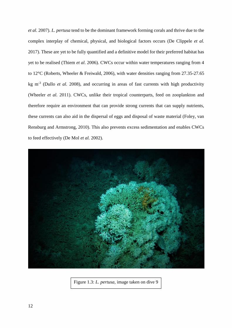
et al. 2009). Figure 1.3 below shows a photographic example of a live L. pertusa specimen,
taken at the Porcupine Bank Canyon. Open slope CWC mounds can be found in the Atlantic
along the Rockall and Porcupine Banks, and these do not occur by happenstance and have been
found to correlate with large scale water mass boundaries (White and Dorschel 2010, Mienis
Figure 1.2 Global Coral Presence (Freiwald et al. 2017)
12
et al. 2007). L. pertusa tend to be the dominant framework forming corals and thrive due to the
complex interplay of chemical, physical, and biological factors occurs (De Clippele et al.
2017). These are yet to be fully quantified and a definitive model for their preferred habitat has
yet to be realised (Thiem et al. 2006). CWCs occur within water temperatures ranging from 4
to 12°C (Roberts, Wheeler & Freiwald, 2006), with water densities ranging from 27.35-27.65
kg m-3 (Dullo et al. 2008), and occurring in areas of fast currents with high productivity
(Wheeler et al. 2011). CWCs, unlike their tropical counterparts, feed on zooplankton and
therefore require an environment that can provide strong currents that can supply nutrients,
these currents can also aid in the dispersal of eggs and disposal of waste material (Foley, van
Rensburg and Armstrong, 2010). This also prevents excess sedimentation and enables CWCs
to feed effectively (De Mol et al. 2002).
Figure 1.3: L. pertusa, image taken on dive 9

13
CWCs establish themselves when a coral larvae colonises an area of hard substrate, all CWC
are colonies that consist of animals named polyps (Wheeler et al. 2011). Once growth has been
initiated, the success of the coral colony largely relies on the aforementioned environmental
controls. Scleractinia are ecosystem engineers that need to outgrow sedimentation and other
destructive forces in order to maintain their 3-dimensional structure that enables their continued
growth as it acts as a foundation for juvenile coral specimens to establish themselves upon in
the future (Maier et al. 2011). If favourable conditions persist over a sufficient period of time
then new coral can grow on the skeletal remains, potentially creating mounds that can be to
350m off the sea floor and extend out over several square kilometres (Mullineaux and Mills,
2006). Coral mounds are made through succession of coral reef development, sedimentation
and erosion, coral skeletal matter may be dissolved over time and will often form a cement to
hold the different elements of the framework together (Wheeler et al. 2011). Whether these
mounds sustain contemporary reefs determines whether they are described as active mounds
(supports live coral specimens) or retired mounds (the framework is dead) (Roberts et al. 2009).
The topography of the seabed has a strong influence on the morphology of the overlying corals
(Wheeler et al. 2011). Corals can occur as a thin veneer along a suited substrate as seen in
several sites along the Gulf of Mexico (Hübscher et al. 2010). Figure 1.4 below displays a
series of antipatharian and scleractinian coral specimens occurring on top of a large dropstone.

14
Historically the CWCs occurring on the NE Atlantic continental margin remain the most
intensively studied (Van Oevelen et al. 2009; Frank et al. 2011; Wheeler et al. 2011; Dorschel
et al. 2009). Observed influences on CWCs vary depending on both the temporal scale being
examined, with second scale turbulences and diffusion to month long tidal regimes and major
oceanographic phenomenon (Navas et al. 2014). Relevant spatial scales vary from cm size
currents flow through and across coral, which affects local biochemical fluxes and skeletal
morphologies to currents that flow across entire reef complexes (Navas et al. 2017). It is clear
that a series of water mass characteristics interact to drive marine ecosystem structure and
Figure 1.4: Antipatharia and Scleractinia Specimens taken
from dive 12.

15
functioning in deep water settings, however the data and models to analyse this drive are
lacking (Flögel et al. 2014). On the Porcupine Bank, a large dome shaped cold water mass has
been observed, this is occurring due to the presence of deep water mixing regime that occurs
over the bank (Mazzini et al. 2011; White et al. 2005; White et al. 2007). Previous studies
indicate that this mixing regime is generated from the interaction of the East North Atlantic
Water (ENAW), a warm saline water mass, and deep winter currents, a distinction thermocline
has been observed at approximately 600m depth (Mazzini et al. 2011).
CWCs can also be affected by long term global changes in climate. Challenger Mound, for
example, occurs within the Belgica Mound Provenance of the Porcupine Seabight, and contains
mounds that appear to have been initiated at least 2.4 ma. Challenger mound also displays
pronounced hiatuses in growth, occurring from 1.7-1.0 ma, with of growth reinitiating shortly
afterwards (Kano et al. 2007). These have been linked with glacial cycles, with a significant
loss in production causing the elimination of most of the fauna within the reef during
glaciations, then during interglacial periods, the mounds continue their previous growth
(Roberts, Wheeler & Freiwald, 2006). As a result, CWC mounds forming in the NE Atlantic
are generated as a sequences of interglacial coral reef framework overlain by glacial hemiplegic
deposits (Roberts and Cairns 2014). Thus, highlighting the profound influence that the
chemical and physical conditions can have on CWC mound evolution, as it is continuously
influenced by the interaction of the hydrodynamic and sedimentary regimes, which is coupled
very closely with the global climate (Henry and Roberts, 2007).
3.3. Ecological & Economic Value of Cold Water Corals
16
In order to determine economic value of CWC corals, ecosystem goods and services provided
by CWCs must first be established (Foley, Rensburg and Armstrong 2008). This includes any
direct or indirect use values; direct use refers to any actual or planned use of a service by an
individual (Bolt et al. 2005). Direct use values are based on stocks or assets, such as coral and
fish biomass and genetic raw materials embodied in organisms, which are sold in markets and
services derived from a CWC area (Foley, Rensburg, and Armstrong 2008). These goods or
services can include value of contracts for commercial seafood products, coral for jewellery,
and organisms and raw materials extracted from CWC sites which are used as inputs by
manufacturing and pharmaceutical industries. CWC coral offer indirect use values, in the form
of environmental regulating services such as temperature regulation, regulation of atmospheric
greenhouse gases, and adsorption of waste and pollutants (Armstrong et al. 2012). Most
importantly, it supports ocean life by the cycling of nutrients and provides a habitat for a vast
array of species (Jobstvogt et al. 2014).
Authogenic ecosystem engineers such as trees or corals generate or alter their habitat through
their presence (Miller et al. 2012). Ecosystem engineers may ameliorate the environmental
conditions, they can transform the biological interactions within a habitat (Cathalot et al. 2015).
CWCs are archetypal authogenic engineers and they provide habitat complexity in otherwise
homogeneous, sedimented environments, augmenting the biodiversity within the area
(Bongiorni et al. 2010). Food web analysis of CWCs in the Logachev Mound complex suggests
that CWCs have a much greater production rate of organic carbon than the surrounding soft
substrate environments, a significant find given the scarcity of food within this part of the ocean
(Van Oevelen et al. 2009).
CWC mounds are hotspots of biodiversity for benthic habitats, an example of this can be seen
in a study of CWCs within the Porcupine Seabight, which yielded 349 species including 10
undescribed species from a total of 7 box cores (Henry and Roberts, 2007). Morris et al. (2013)

17
conducted studies that yielded 855 coral colonies per 100m ROV transect, including 31
individual coral species. Highest taxonomic richness was observed within the L. pertusa reef
habitat (Morris et al. 2013). CWCs are not only significant in terms of local species richness
(α-diversity), their macro habitat heterogeneity ensures that they are also important centres of
spatial turnover in β-diversity (Henry and Davies 2009). Nonetheless, within certain areas of
the world, the role of CWCs in fish species distribution remains unclear when concerning the
influence of multiple drivers occurring over various spatial scales, with studies suggesting that
CWCs role is species specific and not universal across all fauna (Milligan et al. 2016).
CWCs can provide nursery grounds and living space for many different juvenile and adult
species, many commercial fish species take advantage of this commodity and as such CWC
habitats can be vital for fish stock maintenance (Huvenne et al. 2016). Henry et al. (2013) used
video surveys to evaluate spawning grounds for the shark species Galeus melastomus within
the Mingulay Reef Complex off Western Scotland. The findings indicated a greater abundance
of this species was concentrated around the reefs within the area, and individuals were also
noted to be larger than average, indicating that the reef may also provide a feeding grounds for
this species (Henry et al. 2016). Such sharks are valuable species for recreational angling and
their habitat use in coral ecosystems suggest possible environmental synergies, whereby one
ecosystem function is enhanced by another (Bennett et al. 2009).
Tropical corals have gained a prolific status within the conservation community with a wide
range of valuation studies being conducted, identifying these habitats as biomes with the
highest valued ecosystem services in aggregate, emphasising their importance (Sheppard
2013). Their deep-sea counterparts, cold-water corals (CWCs) have been subjected to one
valuation effort, which was largely inconclusive (Glenn et al. 2010). This is surprising given
that 65% of all corals occur below depths of 50m (Lindner et al. 2008).

18
3.4. Threats to Cold Water Corals and their Ecosystems
Currently, the global environment is .in a state of flux with atmospheric and oceanic
temperatures on the rise worldwide causing change that is novel within the realms of human
history (Harsch et al. 2017). As such ecologists recognise the importance of the monitoring
and predicting of this change in order to help curb the catastrophic effects of global warming
(Evans 2012). Coldwater corals (CWCs) are an important reservoir for biodiversity and provide
a refuge and a spawning ground for a whole host of flora and fauna (Ballion et al. 2012), they
also represent a vast store of carbon in the form of calcium carbonate (Foley, van Rensburg
and Armstrong, 2010). Deep water marine environments are characterised by low fecundity,
low productivity, older age at maturity and a high longevity of the species adapted to the
environment, as a result, CWC ecosystems are regarded as being one of the most sensitive deep
marine ecosystems to change (Fabri et al. 2014). CWCs occur within a narrow range of
parameters including temperature, pH, and salinity ranges, consequently, these organisms have
a very low tolerance to environmental change (Goffredo and Dubinsky, 2016).
Current research indicates that ocean acidification and increasing temperatures are threatening
these habitats, with studies indicating that 70% of all scleractinian corals to be exposed to
corrosive waters and temperature increases by the end of this century, this may cause a
significant decrease in their extent and continued growth (Büscher, Form and Riebesell, 2017).
Such changes in the environmental parameters can cause a destabilisation of established CWC
reef systems and an extreme loss in biodiversity. Tittensor et al. (2010) model the suitability
of potential habitats for CWCs today versus what the projected chemistry of the oceans in 2099

19
under the IPCC, IS92a, and S650 scenarios, all of which exhibited a pronounced reduction in
suitable coral habitat. This depletion of coral habitat is not uniform as seamounts were found
to be consistent refuges for CWCs due to higher levels of aragonite saturation (Tittensor et al.
2010).
CWC reefs are vital ecosystems for many types of commercial fish causing significant
concentrations to occur around the reef, currently shallow continental shelf fish stocks are in
decline and fisheries are moving into deeper regions (Husebø et al. 2002). Bottom trawling
remains one of the most destructive impacts on CWC habitats, as heavy metal frames are
involved within the practice and as they are dragged along the sea floor they can destroy exiting
coral habitat (Armstrong et al. 2014). When considering that a normal fishing excursion would
last over 10 days and cover 100km2, trawling within the marine environment has the potential
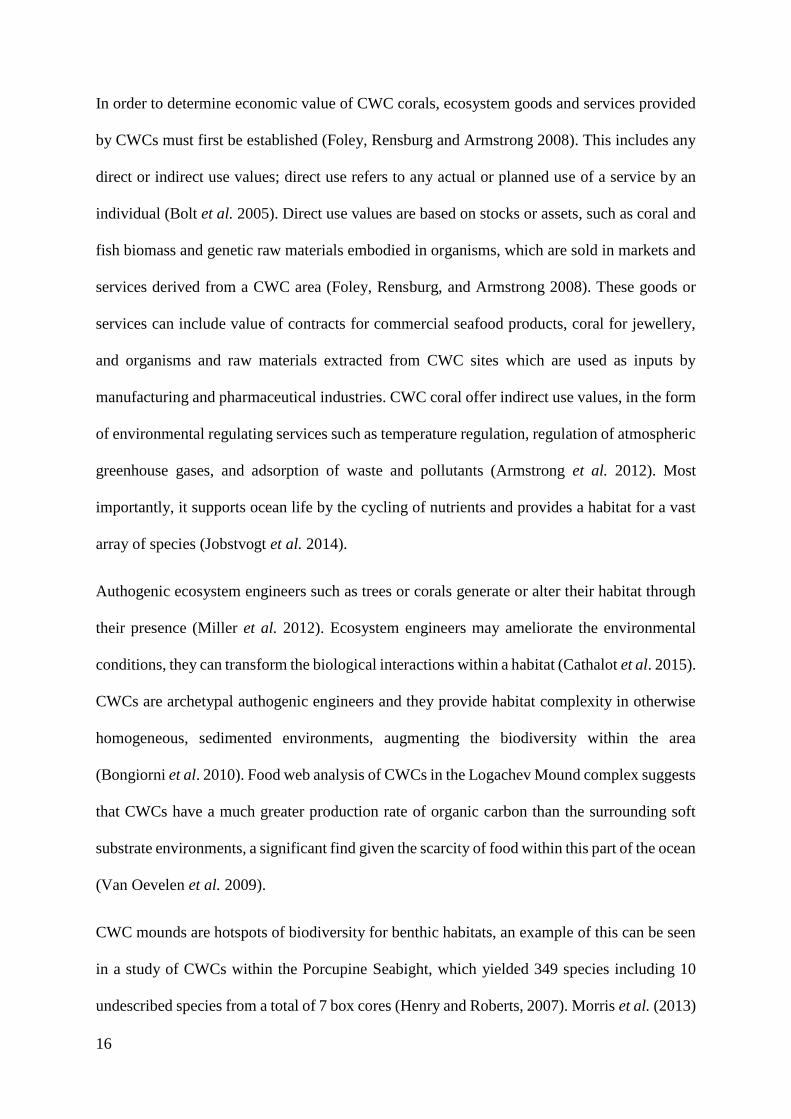
to damage a large portion of CWC habitat, this is illustrated in Figure 1.5 below. (Davies et al.
2007). Such fishing practices can often lead to sediment becoming re-suspended in the water
column, this is detrimental to CWCs as they are suspension feeders and their ability to take in
nutrients can be hampered by the sediment being re-deposited on top of them (D’Onghia et al.
2016). This effect has been observed to impact a much greater area than that of the physical
destruction caused by the trawling equipment. In areas of complicated bottom topography (such
as the Ionian Sea), which remain inaccessible to trawling, threats may come from the use of
other gears such as long line fishing (Sampaio et al. 2012). It is believed that bottom long lines
sweep the sea bed (when gear is hauled up) in a comparable way to demersal trawling
(Kilpatrick et al. 2011).
20
Lastras et al. (2016) conducted a comprehensive video survey on the impacts of bottom
trawling practices on corals within La Fonera Submarine Canyon Head in the Northern
Mediterranean Sea, the survey revealed extensive trawling damage and sea litter. Surveys
conducted studying the differences between unfished and fished seamount habitats in the
Chatham Rise off the coast of New Zealand, this zone is subject to extensive trawling practices
primarily for the exploitation of orange roughy and oreos (Clark and O’Driscoll 2003). Clark
and Rowden (2009) revealed a marked difference in the invertebrate assemblages between
them, with fished seamounts displaying a depleted coral habitat relative to the unfished zones,
the fished zones also exhibited signs of damage created by trawling. L. Pertusa have a skeletal
extension rate of 6 to 26 mm/yr, this had been derived from studies that indirectly examined
the stable isotopes (Mortensen & Rapp, 1998; Mikkelsen et al. 2008; Rogers 1999), and studies
observing corals that were grown on artificial substrate (Gass and Roberts, 2006). Thus, CWC
recovery rate from any form of damage to reef or mound structures is slow, it is often estimated
to take tens of thousands of years for a reef to fully recover, thus CWCs are sensitive to
destructive anthropogenic influences, fulfilling all the requirements to be labelled vulnerable
organisms (Andrews et al. 2005; Foley, van Rensburg and Armstrong, 2010).
Figure 1.5 Coral debris created from demersal trawling, trawl marks are
evident, resulting in complete CWC habitat destruction (Rossi et al. 2017).

21
Similar parallels can be drawn from the recent development of the hydrocarbon industry as
deeper reservoirs are required to sate the globe’s current demand for oil and gas resources,
raising concerns amongst conservationists that CWCs could be smothered by the discharge
(Rogers 1999). While studies have shown that CWCs can adapt reasonably well to an
environment with active near-bed sediment fluxes, exposure to fine sediments and drill
cuttings, they are still measured with a marked drop in skeletal growth (Larsson et al. 2013).
White et al. (2012) conducted surveys on coral communities in the Gulf of Mexico 3-4 months
after the Deepwater Horizon oil spill had occurred, 10 healthy coral communities were
observed at >20km from the initial spill site, however one site at 11km presented with
widespread signs of stress. 46% of 43 corals imaged at the site exhibited evidence of impact
on more than half the colony, manifesting in tissue loss, sclerite enlargement, excess mucous
production, bleached ophiuroids, and covering by brown flocculent material (White et al.
2012).
3.5. Conservation Efforts
One of the biggest challenges with deep marine habitats is raising awareness of the hidden
vulnerability and diversity of these corals, as CWC are seen as a novelty (Huvenne et al. 2016).
A dichotomy exists between the need to preserve biologically diverse habitat and maintaining
economically lucrative fish stocks, as CWC habitats have been found to support large
populations of economically viable fish stocks (Henry et al. 2013). Understanding the
processes that drive species distribution and the scale at which these processes operate is of
vital importance, particularly when the species is of a high conservation or commercial value
(Milligan et al. 2016). CWCs have been found to be vital to species specific faunal

22
assemblages, and are now recognised as being threatened at the levels of species, habitat (e.g.
trawling damage) and ecosystem (e.g. ocean acidification) (Huvenne et al. 2016). Efforts
focusing their conservation through the designation of protected areas (MPAs), where activities
such as bottom fishing with towed nets and dredges being restricted (Roberts and Cairns 2014).
These MPAs have the potential to protect both CWC habitat and fish stock and are the most
suitable solution with especially when dealing with areas where enforcement and compliance
costs and would outstrip any potential economic output (Foley et al. 2010). MPAs can be
enforced on a wide range of levels from complete closure of the area, restriction of fishing gear
used, to zoning approaches where different activities are banned from different zones (Foley et
al. 2010). Implementation of MPAs in shallow sea environments have shown widescale
improvement with increased abundance and lifespan of individual species and a greater
connectivity within the environments displayed, it is believed that enforcing MPAs in deeper
marine environments will have a similar effect and aid in the recovery of CWC ecosystems
(Davies et al. 2007).
Huvenne et al. (2016) conducted a study 13 year after a deep fisheries closure and MPA at
approximately 1000m depth had been imposed at the Darwin Mounds in the NE Atlantic in
1998, this was an area that had been subjected to bottom trawling practices. Results show that
areas that largely avoided disturbance showed similar levels of coral presence as had been
found in 1998, however areas in the eastern portion of the Darwin Mounds maintained a
desolated habitat with no recolonization and lack of growth of the corals (Huvenne et al. 2016).
This highlights the need for a proactive approach to CWC conservation as the slow growth rate
for CWCs exhibits the lack of resilience that these organisms have to drastic and invasive
changes to their environment (van Rensburg and Armstrong, 2010). Armstrong et al. (2014)
postulates that many of the protected areas delineated for coral reef are designated based on the
fact that coral habitats are unique zones within the marine environment, with most areas being

23
chosen due to limited impact on fisheries, rather than maintaining an emphasis of conservation
for the species. It is therefore imperative to prioritise CWC and to integrate a comprehensive
policy of conservation that is inclusive, whose processes are accessible for stakeholders in a
marine zone (Stillman et al. 2016). Ross and Howell (2012) utilised predictive habitat
modelling to assess the suitability of predictive habitat modelling when delineating Marine
Protected Areas for listed coral species, concluding that these models enabled prompt
assessment of potential habitats. Predictive habitat models have been employed in the
assessment of spatial closures for CWCs on the landings of economic fish species in the Hectat
Strait, in British Columbia, here estimations show that if 99% of coral reef habitat were closed
off for protection, this would reduce landing values to 63% (Largasse et al. 2015). These
models also provide a simple and straightforward means that allow local stakeholders to
visualise and comprehend the significance and extent of habitats, enabling more effective
management and inclusion of natural resources (Stillman et al. 2016).
3.6. Predictive Habitat Modelling
Predictive habitat modelling has proven itself a valuable tool in quantifying, evaluation
governing, and conservation of natural resources and is the basis of many studies on a wide
variety of species ranging from those native to tropical rainforest climates to cetacean research
(Hansen et al. 2015; Lambert et al. 2014). Predictive habitat models have also played a vital
role in prioritising areas for conservation and scientific research (Ross and Howell 2012).
Therefore, it is critical to ensure that these models are made to the highest quality possible
However, it is clear from the research that much of the data theoretical and that field
observations and surveys are needed to ground truth this data and ensure increased accuracy of

24
these models (Davies et al. 2008; Davies and Guinotte 2011; Guinotte and Davies 2014). This
is limited by the high costs associated with sampling and surveying the deep sea, making it
economically infeasible to maintain detailed survey data of all the world’s oceans (Davies and
Guinotte 2011).
Ecological Niche Assessment has been an essential part of establishing predictive habitat
models and has been extensively applied to CWC habitat prediction, establishing global and
regional CWC habitat models (Davies et al. 2008; Dolan et al. 2008; Yesson et al. 2012;
Guinan et al. 2009). Executed through the intense scrutiny of presence records and their
relationship with the physical parameters occurring within the environment (Mc Nyset 2005).
Ecological Niche Assessment relies on understanding the factors influencing species
distribution, and this can be done over multiple scales (Guinan et al. 2009). GIS based
techniques and statistical methods (Ecological Niche Factor Analysis) have been included in
these assessments in past studies (Zhao et al. 2006; Hirzel et al. 2006). A common component
within these models is the incorporation of georeferenced presence data in combination with
environmental variables that ultimately culminate in a map which delineates areas of potential
species coverage (Guinan et al. 2009). Presence data can be derived from museum records
(Lim et al. 2003), atlas collections (Peterson 2001), and field samples (De Clippele et al. 2017).
Environmental variables are obtained as those variables that may influences the ecological
niche within which the species occupies and are not variables that would change with time.
Historically Ecological Niche Factor Analysis (ENFA) was one of the most successful methods
of predictive habitat modelling for terrestrial and marine habitats (Dolan et al. 2008). ENFA
employs a suite of variables, Eco Geographic Variables (EGVs), and relates them to species
distribution data to create a habitat suitability model (Freiwald and Roberts, 2005). Regardless
the quality of the input data that is used remains the controlling feature within a habitat
suitability model, with challenges arising from poor data sampling techniques often caused by

25
a lack of concern for experimental design (Guinan et al. 2009). Many studies involve the
manual weighting of EGVs based off independent variables that are specific to the area, and as
such are only suited to best fit the specimens limited within that survey site (De Clippele et al.
2017). Success applications of the technique have been applied to CWC modelling using
presence only data mostly with global distributions (Davies et al. 2008).
Maxent (Maximum Entropy Models) based models that use presence only data now have
surpassed the traditional ENFA based approach and have produced models that give a more
exact position of CWC habitat, a comparison that has recently come to light (Davies et al.
2011; Tittensor et al. 2009; Ross and Howell 2012). Davies and Guinotte (2011) displays the
difference in resolution between a previous model created through Biomapper utilising ENFA
presence based analysis and a Maxent model utilising presence only data (Davies et al. 2008),
Figure 1.6 below displays resolution improvement between the 2 models.

26
UNEP CWC presence database represents the most complete record of CWC distribution
across the globe, and has been utilised by many studies as parameters for CWC occurrence
globally (Yesson et al. 2015; Davies and Guinotte 2011). Yet some of the coral positions that
are included within this data are taken from data that has yet to be groundtruthed (A., J.,
Figure 1.6: Davies and Guinotte (2011) show the increase in resolution between the current
model, Map (a) and previous global distribution models, Map (b) (Davies et al. 2008).

27
Wheeler, Personal Communication, 31st August 2017). suggesting possible political factors
interfering with the authenticity of the dataset and the accuracy of predictive habitat models
that include this data within their parameters (Dorschel et al. 2010).
4. Materials and Methods
4.1. Study Site
The Porcupine Bank is dominated by the East North Atlantic Water (ENAW), which originates
from the Bay of Biscay and enters the Rockall Trough from the south east and is carried
northwards by the Continental Slope Current (Pollard et al. 1996; New, Smith and Wright
2001). The ENAW ranges between 200-700m (White and Dorschel 2010) and is underlain by
the Mediterranean Outflow Water (MOW), which enters the Rockall Trough from the south
according to CTD and boundary layer data collected in the north of the Porcupine Bank (Mienis
et al. 2007). A steep pycnocline exists between the MOW and the ENAW (Morris et al. 2013).
The MOW extends to 1200m in depth where is interacts with the Labrador Sea Water, this has
a maximum salinity at 1800m in depth and its signature ends at 1900m, hereafter there are
many water masses that occur in small amounts (Van Rooji 2004). Bottom current, salinity and
temperature profiles of this area show a clear semi diurnal cyclicity, with salinity ranging from
35.2-35.4%, temperatures ranging from 7-9°C, and current speeds ranging between 10-20ms-
1, sometimes reaching speeds of 30ms-1 (Mienis et al. 2007). Current speeds from a deeper
reference site (2500m bsl) reached less than 10ms-1 (Mienis et al. 2007). Sedimentological

28
studies also confirm the increase in bottom current speeds towards the coral carbonate mound
range (Øvrebrø et al. 2006).
4.2. ROV-Video Data Collection
During the CoCoHaCa ROV survey (2017) on the ILV Grainuile, video data was captured via
composite video with the Holland 1 ROV (cruise number RH17002). Positioning and
navigation were acquired through the deployment of a USBL (Sonardyne Ranger 2) and RDI
Workhorse DVL. The altimeter on the ROV recorded and logged the height of the ROV from
the seabed. Video and photographic data was captured through a digital stills camera mounted
on the ROV facing towards the seabed. This data was recorded in transects that ran roughly
west to east over the eastern wall of the Porcupine Bank Canyon, with the ROV maintaining a
2m distance from the sea bed or mound surface. The positions of these dives are outlined in
Figure 1.7 Appendix I. The ROV roughly began at the foot of an incline and gradually
continued up the slope and terminated at higher ground. This data was used to ground truth the
pre-existing coral presence data provided by UNEP and to help validate the models that have
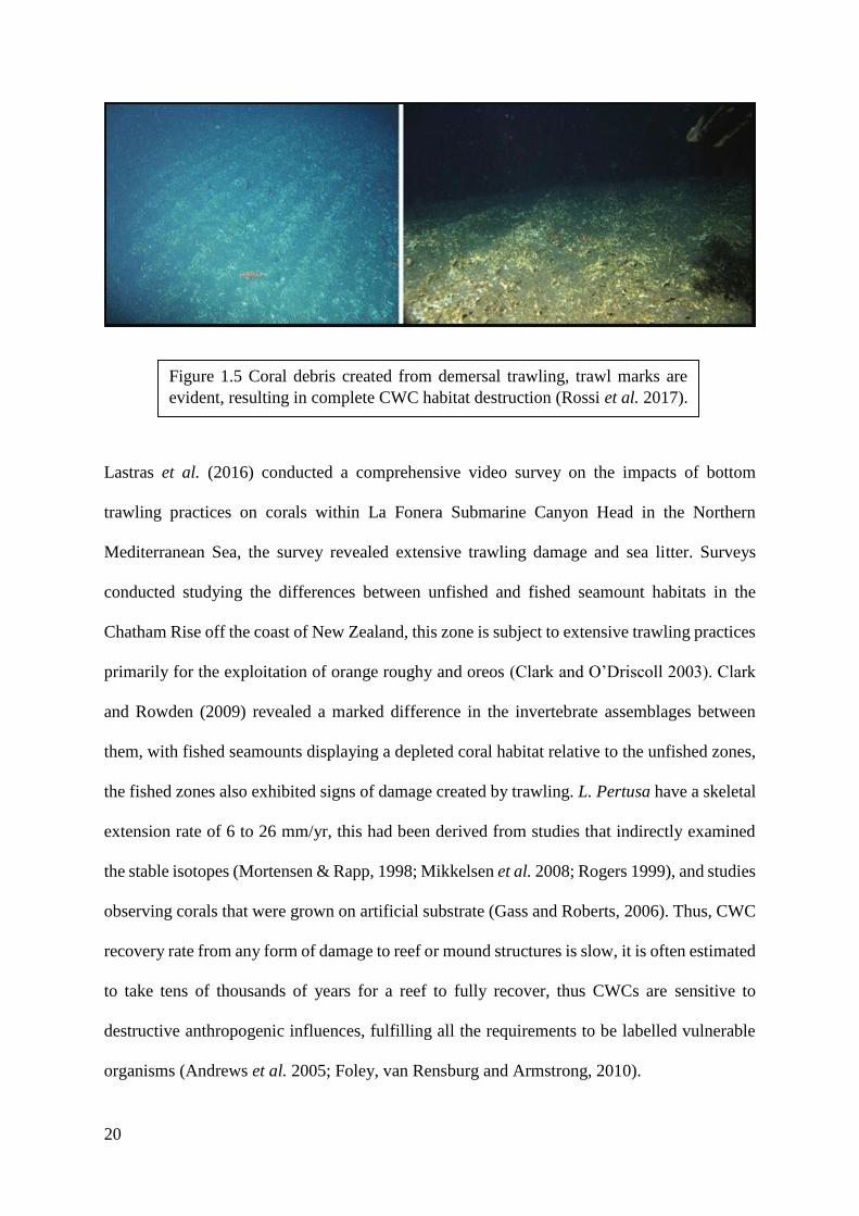
been presented in previous studies (Davies et al. 2011). Figure 1.8 shows a sideview of the
ROV Holland I.
29
4.3. Seabed Classification
A georeferenced video catalogue of the seabed surface had been created using a seabed
classification scheme that had been adopted from antecedent research that assesses ROV dive
based facies classification (Lim, Wheeler and Arnaubec 2017; Dorschel et al. 2007;).
Processing of the video data required a manual classification scheme to be employed, as neither
a supervised nor an unsupervised classification scheme could be employed as a consistent
height could not be maintained by the ROV off of the seabed. The facies classifiers chosen
were: “Live Coral Framework”, “Dead Coral Framework”, “Soft Corals”, “Hard Coral
Individuals”, “Hemipelagic sediment” and “Bedrock”. This seabed classification scheme was
Figure 1.8: ROV Holland I recovering onto deck
(Marine Institute)

30
complemented by USBL navigation data that headed the top of the video display, allowing for
time capture measurements of seabed change to be noted. These observations were noted in
excel, sea bed facies changes were noted immediately, and were merged with OFFOPS GPS
coordinates by matching the times of the observed facies changes with the corresponding
coordinates, allowing for quantification of the CWCs and their habitat. A test of the
classification scheme was run over dives 1 and 2 to amend any previous classes and calibrate
the classes. An example of the classification scheme can be seen in Table 1.0 below. Hard coral
facies classes were the facies used to validate the model as they create the 3 dimensional
framework that is central to CWC importance.
Class Facies
1 Live Coral Framework (LCF)
2 Dead Coral Framework (DCF)
3 Soft Coral
4 Hard Coral Individuals
5 Sediment
6 Coral Debris
7 Bedrock
8 Miscellaneous
Table 1.0: Seabed Facies classes

31
LCF facies was used to label coral reef that had living coral specimens growing on top of a 3
dimensonal framework, i.e. that come together to form an active reef or mound. Dead Coral
Framework consisted of dead CWC skeleton which had not been further colonised by new
CWC, video analysis determined that there are no living parts. Soft coral faceis were designated
for seabed dominated by antipatharians. Hard Coral facies was reserved for those individual
coral specimens that are in the initial stages of growth and have not come together to form one
cohesive framework. Sediment facies was designated for those habitats that were dominated
by hemipelagic sediment. Coral debris facies was designated for carbonate rubble, that
included recognisable biogenic material (i.e. coral rubble and shell fragments) and sediment.
Bedrock facies was for exposed bedrock that occurred along the sea floor, including only rock
that consisted of the underlying bedrock, excluding regolith (such as hemipelagic sediment and
dropstones). Miscellaneous was used to indicate the areas where the seabed had no longer been
in sight of the ROV. All facies were designated once they achieved cell coverage (video frame
coverage) of >50%. Any changes in the seabed were immediately documented and the position
noted. Examples of facies 1-7 can be seen in Figure 1.9 below.

32
(A)
AA
AA
AA
A(
A
(B)
(C) (D) (E) (F)
Figure 1.9: Examples of the predominant Seabed Facies: (A) Bedrock, (B) Coral debris,
(C) Antipatharians (soft coral), (D) Live Coral Framework, (E) Hemipelagic sediment, &
(F) Dead Coral Framework.
(C) (D)
(E) (F)

33
4.4. Environmental Parameters
A CTD profile had been recorded at the start and end of each dive to create a record of the
environmental conditions of the water column and to help identify possible water mass
changes. CTDs 1-39 and CTDs 44-49 were taken through the ROVs on board CTD sensor,
with the depths ranging from 560-1254m water depth. CTDs 40-43 were collected using a
Seabird SBE 911 profiler, which included sensors for temperature, conductivity and dissolved
oxygen, as well as a transmissometer. The CTD was deployed without the use of a rosette to
ensure speed of capture. They were taken at depths ranging from 1180m to 1794m. CTD
collection occurred at the beginning and end of each dive, with the downcast occurring as the
ROV was lowered into the water, an upcast was taken upon its retrieval.
CTD data was imported into ArcGIS to assess any potential correlations with the coral presence
data and to eliminate any parameters that have no effect on the distribution of CWCs within
the area. All ROV CTDs were taken at 2m away from the seabed, all SBE CTDs were taken at
depths of 10m off the seabed to avoid damaging the equipment. CTD raw data files were
processed through the SBE Data Processing software, they were first converted to *cnv. files,
and in order to enter them into ArcGIS software effectively they were bin averaged to 1m. The
*cnv. files were imported into excel and the data was separated into tables, then plotted using
Grapher 8 in order to recognise different water masses within the vertical column. CTD
Locations are included in Figure 2.0 in Appendix I. A picture of the Seabird SBE 911 CTD
profiler can be seen in Figure 2.1 below.

34
4.5. ROV-Borne Multibeam Echosounder (MBES)
ROV mounted MBES data was collected over the Porcupine Bank Canyon as part of the
QuERCI I Survey (2015), this was conducted on board the RV Celtic Explorer, with the
Holland I ROV. A high-resolution Kongsberg EM2040 MBES was mounted on the front of
the ROV and this acquired data at a frequency of 400 kHz. The survey travelled at a speed of
2 knots with the ROV maintaining a distance of 30m off of the seabed. A sound velocity probe
had been integrated with the MBES and the positioning and attitude of the ROV were procured
by using a Kongsberg HAINS internal navigation system, ultra-short baseline (USBL) system
(Sonardyne Ranger 2) and doppler velocity log (DVL). These combined with the dGPS on the
Figure 2.1: CTD Profiler, without Rosette

35
ship produced a MBES grid that was imported into Arc Map 10.4.1 at a 10cm grid size. The
loss in temporal resolution with regards to this dataset is offset by the longevity presented by
CWCs and their slow growth relative to other marine organisms (Fabri et al. 2014).
INSS bathymetry data of the Porcupine Bank Canyon was used as a lower resolution dataset
that included all the coral presence data, a second dataset was acquired to apply the weights of
the 2 models to the entire Porcupine Bank to discern any further areas of CWC coverage.
4.6. Analysis of Catalogue Data
The video data catalogue was imported into ArcMap 10.4.1 and was then inserted into a map
that had bathymetry collected from both the ROV-borne MBES (10m Cell size) and a lower
resolution dataset (35m cell size). Acquisition of the lower resolution bathymetry was done
through NOAA website through the multibeam portal. This data was provided by the INSS
through hull mounted multibeam surveys of the Porcupine Bank, these surveys are the most
complete view of the Irish seabed and allowed for a comprehensive study of the Porcupine
Bank Canyon. As the ROV-borne MBES had been collected in UTM Zone 28, the bathymetry
taken provided by the INSS was converted to this projection using the project raster tool in
ArcMap. Slope (Degrees) and aspect profiles for both datasets were then generated through the
Arc Toolbox Spatial Analyst Tools.
Once the video catalogue data had been acquired for the various dives they were synchronised
with the navigation from the ROV and filtered so that it only displayed the location data for
the corals. The high spatial resolution data was utilised for dives 8, 9a, 13, 14, 15, 16, 17, 18,
18a, 19 and 20 as they are the only dives to occur completely within the higher resolution
dataset area. The lower resolution data was used for all dives within the survey (e.g. Dives 1-

36
20) to ensure that there was one uniform dataset for the entire catalogue. The location data from
the ROV had been acquired through OFOBS software, however dives 6, 9, 12, 13, 14, 15, 17,
18, and 18a were missing and so the raw navigation files were pulled from the ROV and were
processed. Consequently, these dives were recorded in UTM Zone 28, whereas the other dives
were recorded in WGS 1984, to ensure the highest accuracy possible and to simplify the
measurements, both datasets were exported as *shp. files and converted to UTM Zone 28 using
the project tool. Once correctly georeferenced, slope and depth values were obtained using the
extract values tool.
4.7. CTD Processing
CTD data was plotted on ArcGIS, by extracting the data as to only include the data for the
maximum and minimum coral depth values. This data was further broken down into 4 separate
depth zones, that correspond with the preferred depth zones seen in Davies and Guinotte
(2011). They also correspond with the maximum and minimum values observed in the hard-
coral presence data. Graphs depicting the environmental conditions within each CTD can be
found in Figures 2.2 to 6.8 in Appendix II.
Averaging of the data allowed for effective interpolation to ensure effective averaging of the
data and prevent overloading the model with data. However, this averaging has also assumed
much of the coverage within the model area and thus reducing the spatial accuracy and the
originality of the data. Interpolation was done at a resolution of 80m, this was the most
precision resolution achievable with the data whilst keeping a uniform resolution across all
depth zones. Salinity, dissolved oxygen, and temperature were determined from the literature
to be the most significant criteria and were included in this process (Flögel et al. 2014; Dullo
37
et al. 2008; Davies et al. 2008). The raster interpolate toolset was used to interpolate the data
to create a raster dataset for each parameter. In order to avoid any further averaging of the data,
the Nearest Neighbour interpolation tool was implemented to generate this raster dataset.
4.8. Davies and Guinotte (2011) Model Assessment
These criteria were then weighted, based on the values stated within Davies and Guinotte
(2011). As L. pertusa were the dominant CWC observed within the survey site, and they are
the most important framework their values were the ones included within the recreation of the
model (De Clippele et al. 2017). However, certain criteria (Aragonite Saturation and Turbidity)
had to be excluded from the construction of the model as the equipment used within the survey
was not capable of measuring their parameters. Any values that occurred outside the constraints
of the data sets attained were excluded also, as they did not apply to the survey area.
Frequency analysis, as previous mentioned, was applied to the depth and slope values through
the reclassify tool was used to create individual raster files. These were subsequently combined
and weighted, through the map algebra tool, according to observed trends to create idealised
terrain parameters for CWCs within the area. Slope was weighted with greater significance, as
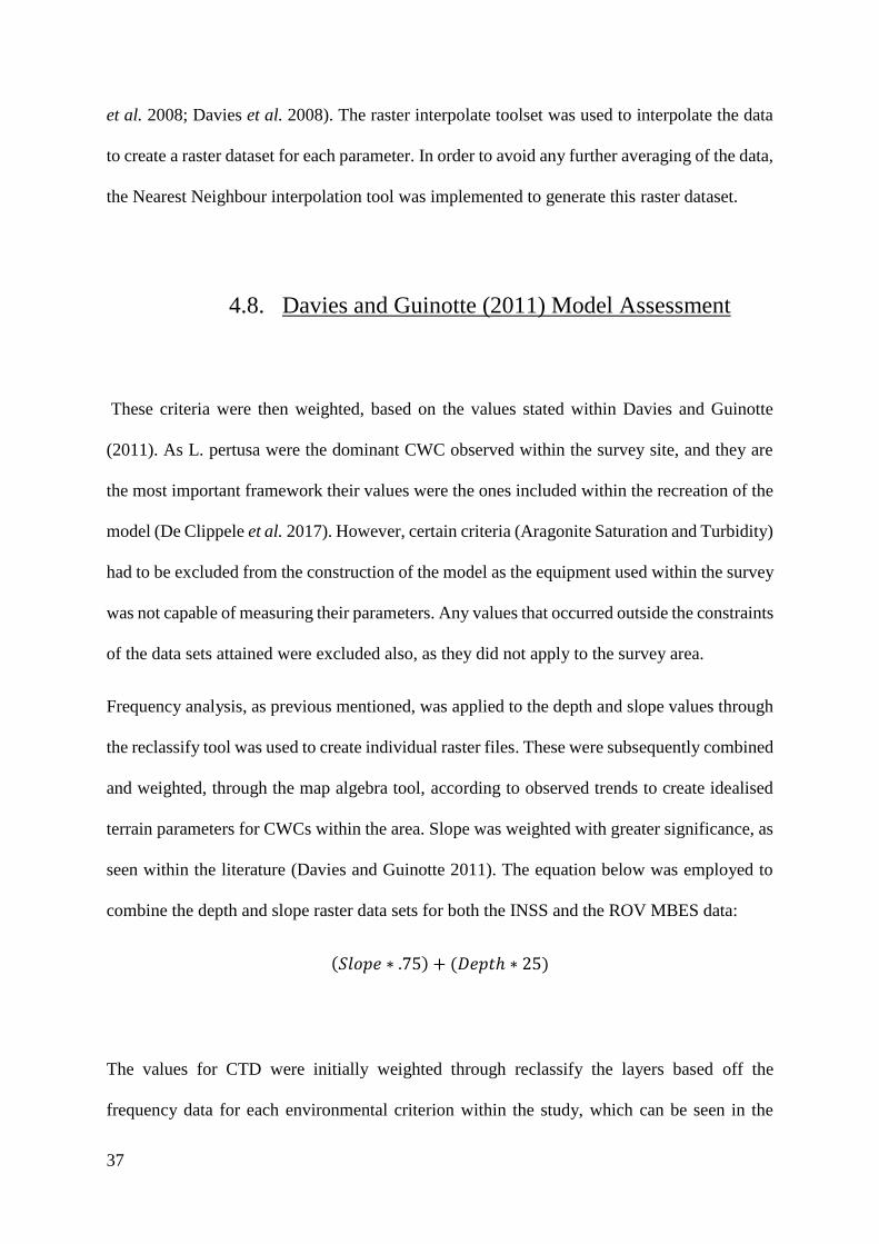
seen within the literature (Davies and Guinotte 2011). The equation below was employed to
combine the depth and slope raster data sets for both the INSS and the ROV MBES data:
(𝑆𝑙𝑜𝑝𝑒 ∗ .75) + (𝐷𝑒𝑝𝑡ℎ ∗ 25)
The values for CTD were initially weighted through reclassify the layers based off the
frequency data for each environmental criterion within the study, which can be seen in the

38
appendices (Davies and Guinotte 2011). This was done for depth ranges 1100-900m, 900-
600m, and 600-0m which were determined through distribution analysis in terms of depth. The
Map Algebra formula used to combine these 3 layers was as follows:
((1100𝑚 − 900𝑚)𝐸𝑣 ∗ .4) + ((900 − 600)𝐸𝑣 ∗ .267) + ((600 − 0)𝐸𝑣 ∗ .333)
(Ev= Environmental variable)
Once this had been done, the physical and the chemical parameters were combined both
through map algebra to create an overall model from both the MBES and INSS data. Both
models were compared with a previous model for CWCs by applying the same criteria stated
within the study (Davies and Guinotte 2011). The values for hard corals were then
superimposed on this model and values were extracted to view where these points occurred
within the model and how this compares with a model created using the frequency distribution
of the CWC presence data. The tables for the weights assigned can be seen in Table 1.1-1.6. in
the Appendices.
Graphs displaying the distribution of L. pertusa for some of the model criteria are included
Below in Figure 6.9.

39
5. Results
5.1. Video Catalogue Classification
The video data had been captured over a series of 20 randomly plotted dives which amassed to
approximately 56 hours of video data which amounted to 53 km of video transects, which were
run between depths of 568m to 1426m in depth. Dive1-12 were taken initially, going from
Figure 6.9: Environmental Variables for L. pertusa
(Davies and Guinotte 2011).

40
North to South. Dives 13-20 were taken with return journey northwards. A map of the resulting
catalogue data can be observed in Figure 1.8 in Appendix I. CWC cover was not constant and
significant portions of each dive consisted of sediment cover tends to generally dominate the
seabed facies for the canyon. CWC presence was first noted in dives 1 and 2, with coral
presence occurring at the beginning of both dives. Figure 7.0 below illustrates a close up of the
catalogue data for these dives. These areas of CWC presence are made up significant, elongate
carbonate mound structures with a rough north east to south west alignment. The main
scleractinians observed throughout the survey were Lophelia pertusa and Madrepora occulata.

41
After dive 2 CWC were largely absent, with no hard-coral facies observed between dives 3 and
5, with soft coral colonies being the only CWCs identified. This can be observed in Figure 7.1
Fig 7.0: Seabed Facies Cover for Dive 1 & 2
superimposed over the INSS Slope Data.

42
below shows the lack of CWC presence within these dives. Antipatharia typically occurred at
greater depths than the Scleractinia, with small colonies of antipatharia often preceding large
CWC mounds.

43
Figure 7.1: Seabed facies data for dives 1 to 6.

44
Hard Coral seabed facies had not been noted again until dive 6. These occurred as sporadic
reefs that did not constitute established mound structures. Large carbonate mounds began
reappearing at dive 9. This dive had the most established CWC reefs and consisted of a large
L. pertusa specimens, see Figure 7.2 below.

45
Figure 7.2: Seabed facies plotted over slope data.

46
LCF was more common along topographic spurs and less common in gullies as is evident in
Figure 7.2 above. Soft Corals tended to occur in large numbers along the wall of the escarpment
to starting at dive 20. Coral presence within the flat areas between mounds was largely absent,
with exception noted at dives 1, 10, 11 and 12. Sedimentary features such as sand ripples and
scouring had been observed in dives 1-6 and dives 10-12, an example of the sediment rippling
is shown below in Figure 7.4.
Fig 7.4: Taken from Dive 2, clear asymmetrical rippling.

47
Dives 1-6 and dives 10-12 also contained dropstones that ranged anywhere from boulders to
cobbles some of which were angular and had a low sphericity. Scouring was evident around
these dropstones, displayed in Figure 7.5 below.
Total lack of CWC coverage was noted at dive 10 with CWC presence returning at dive 11.
The coverage to the south of the mapping area can be seen in Figure 7.6 below:
Figure 7.5: Taken from Dive 10, showing a clear gouge
mark developed from scouring around the dropstones
occurring Orientation is roughly North East to South West.

48
Figure 7.6: Illustrating seabed cover facies for dives
10-12 superimposed over the INSS slope data.
49
5.2. Environmental Parameters
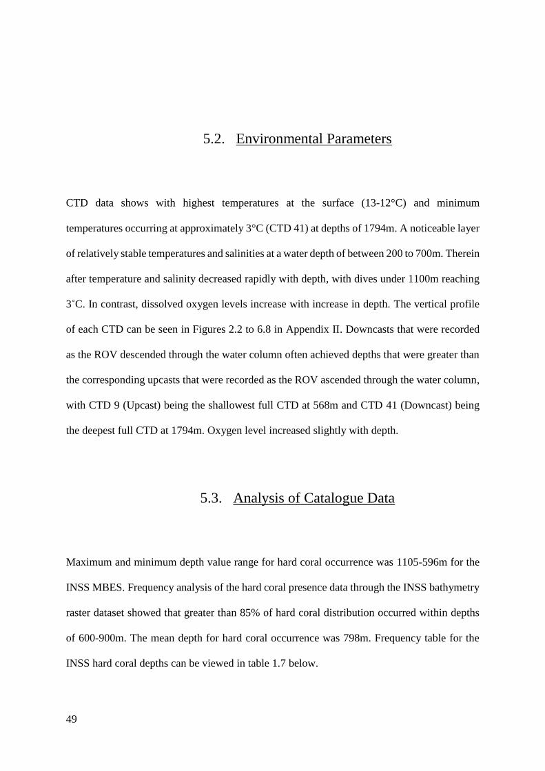
CTD data shows with highest temperatures at the surface (13-12°C) and minimum
temperatures occurring at approximately 3°C (CTD 41) at depths of 1794m. A noticeable layer
of relatively stable temperatures and salinities at a water depth of between 200 to 700m. Therein
after temperature and salinity decreased rapidly with depth, with dives under 1100m reaching
3˚C. In contrast, dissolved oxygen levels increase with increase in depth. The vertical profile
of each CTD can be seen in Figures 2.2 to 6.8 in Appendix II. Downcasts that were recorded
as the ROV descended through the water column often achieved depths that were greater than
the corresponding upcasts that were recorded as the ROV ascended through the water column,
with CTD 9 (Upcast) being the shallowest full CTD at 568m and CTD 41 (Downcast) being
the deepest full CTD at 1794m. Oxygen level increased slightly with depth.
5.3. Analysis of Catalogue Data
Maximum and minimum depth value range for hard coral occurrence was 1105-596m for the
INSS MBES. Frequency analysis of the hard coral presence data through the INSS bathymetry
raster dataset showed that greater than 85% of hard coral distribution occurred within depths
of 600-900m. The mean depth for hard coral occurrence was 798m. Frequency table for the
INSS hard coral depths can be viewed in table 1.7 below.

50
Hard Coral INSS Depth Distribution
Range(m) Frequency %Total
500 to 600 90 0.44
600 to 700 5729 27.83
700 to 800 7524 36.54
800 to 900 4311 20.94
900 to 1000 2416 11.73
1000 to 1100 519 2.52
1100 to 1200 0 0
Extraction of the slope values from the INSS slope data for the hard coral locations showed
that approximately 94% of all hard coral locations had been noted within slopes of 0 to 0.52
radians. With corals displaying a maximum value of 0.89 Radians and a minimum value of
0.025908 Radians. The mean derived from this data was .31 Radians. Table 1.8 below displays
the percentage frequency for the slope data extracted from the INSS MBES.
Table 1.7: INSS depth reclass
frequency distributions.

51
Hard Corals INSS Slope Distribution
Range (Radians) Frequency % of Total
0 to 0.175 5365 26.05760357
0.175 to 0.35 7443 36.15037156
0.35 to 0.52 5400 26.22759726
0.52 to 0.7 1261 6.124629657
0.7 to 0.87 1079 5.24066249
0.87 to 1.05 41 0.199135461
1.05 to 1.22 0 0
1.22 to 1.4 0 0
1.4 to 1.5707965 0 0
Depth values for hard corals extracted from ROV MBES bathymetry data show frequency
distributions of 63% for depths ranging between 600 to 900m depth for hard corals. The
corresponding maximum depth and minimum depth values occur between 1095-659m depth.
The mean depth value for this data set was 839m. The full data depth distribution can be seen
in Table 1.9 below:
Table 1.8: Hard Coral Frequency
Distribution for INSS Bathymetry Data

52
Hard Coral Depth Distribution ROV MBES
Range Frequency % of Total
1300-1200 0 0
1200-1100 0 0
1100-1000 491 7.35
1000-900 1826 27.32
900-800 1698 25.41
800-700 1597 23.90
700-600 1071 16.02
The ROV MBES slope raster showed that 72% of hard coral distribution occurred within values
of 0.5 to 1.2 Radians. With 28% hard coral locations occurring within the range 0 to 0.5
Radians. The maximum and minimum slope values for the ROV MBES slope are 1.154984
Table 2.0: Depth Distributions for Hard
Corals derived from ROV MBES.

53
and 0.111014 respectively. The distribution frequency values for this data is shown in Table
2.1 below:
Hard Corals ROV MBES Slope
Distribution
Range (Radians) Frequncy
% of
Total
0 0 0
0.17 41 0.7442367
0.35 333 6.0446542
0.52 1113 20.203304
0.7 1465 26.592848
0.87 1136 20.620802
1.047 279 5.06444
1.22 1142 20.729715
1.4 0 0
1.57 0 0
Figure 7.7 below illustrates the distribution of hard corals with regards to the aspect of the
terrain derived from the INSS MBES data and the ROV MBES data. Hard corals show a
distribution of 64% for those slopes that dip in a west to north west direction in the INSS data
set.
Table 2.1: Illustrating ROV
MBES Hard Coral Frequency

54
5.4. Davies and Guinotte (2011) Analysis
5.4.1. INSS MBES
This included values for CWC depth, as CWC depth frequency values were included up to a
maximum depth of 2252m and a minimum depth of 453m for the INSS data. Similar constraints
prevented full inclusion of the slope weight values as the maximum slope observed included
occurs at 1.13 Radians in the INSS data. Thus, observations for any values beyond these ranges
could not be made.
Figure 7.7: Aspect for the INSS MBES (A) and the ROV MBES (B).
(A) (B)

55
The terrain data shows moderate initial success within the INSS bathymetry dataset as
considering that the final terrain component of the model had 66% of the total hard coral
presence data occurring within areas that were projected to have a probability of 61% to 90%
of hard coral occurrence. 25% of the hard coral presence data occurred within areas that were
projected to have 40 to 60% probability of hard coral occurrence. However, within 90-100%
probability bracket, only 8% of the total Hard Coral presence data occurs within.
For the final model, displayed in Figure 7.8 in Appendix IV, including the variables derived
from the CTD data, 71% of all CWC data occurred within the 41-62% range. 15% of all hard
coral presence values occurred within the 83% to 100% range. The remaining 13% occurred
within probability range of 20-41%. The results of this analysis Is included in Table 2.2 below:
Davies Probability Analysis
Probability Frequency % of Total
0 0 0
21 0 0
42 703 13
63 3842 71
83 816 15
100 28 1
Table 2.2: Probability frequencies for
Davies and Guinotte (2011) final
model.

56
5.4.2. ROV MBES
The maximum and minimum values for the depth data acquired from the ROV MBES were
2043m and 563m respectively. The average depth of hard corals was 839m water depth. The
maximum value for Radians in the ROV MBES was 1.46 Radians. With an average slope of
.71 radians. The model itself can be viewed in Figure 7.9 Appendix IV.
ROV MBES showed similar numbers displayed within the INSS multibeam data with regards
to the final model with 62% of hard coral presence data occurring within probability range of
41-62%. 18% of hard coral presence data occurs within the probability range of 21%-42%. All
values can be seen in Table 2.3 below:
Davies and Guinotte (2011) ROV MBES
Weighted
Value
% Probability
Range Frequency
% of
Total
20 0 0 0
22.5 0 to 21 0 0
25 21 to 42 974 18
27.5 42 to 63 3355 62
30 63 to 83 937 17
32 83 to 100 123 3
Table 2.3: ROV MBES final model

57
6. Discussion
6.1. Video Catalogue Data
Initial findings within the data show that there are 2 main habitat types, Type (1), CWC occur
on carbonate mounds that occur on gentle slopes along the sides of the canyon, here L. pertusa
tends to dominate. This is predominately found to the North and South of the area with the
corals occurring along elongated carbonate mounds that are roughly aligned North East to
South West. These habitats can be found in Figure 8.0 below.
Figure 8.0: Dives 10-12 (A) and dives 1-5 (B) are plotted over the
slope (Radians) and make up Habitat Type 1, occurring on carbonate
mounds, CWCs occur on the steeper regions of these mounds.

58
The 2nd habitat type had been broken up into 2 sections: Type 2 (a), where CWC are found
along steep sided cliffs of exposed bedrock, here Antiparthia dominate; and Type 2 (b) where
cold water corals are found on carbonate mounds, similar to those seen in Type (1), along flat
areas along that occur on the tops of habitat Type 2 (a). These habitats are illustrated in Figures
8.1 & 8.2 below. Overall coral coverage is not constant and coral debris and sediment facies
make up the majority of dives 3, 4, 5 & 10. LCF was more common along spurs that occurred
along the sides of the Porcupine Bank Canyon, with DCF and coral debris occurring with the
gullies that lay in between. Coral debris tended to dominate in Habitat 2 (a), were it often
occurred at the bottom of cliff faces or down the sides in crevices.

59
Figure 8.1: Here the hard corals (red points) are
overlain on the INSS slope raster, 2 main CWC
habitats occur Habitat 2 (a) occurring as steep
escarpments that coral reef cling to, exposed
bedrock is most common, often occurring as
sheer cliffs, with soft corals attached. Habitat 2
(b) can be observed as the mounds that occur
within the flat areas that appear after the steep
cliff habitats observed in Habitat 2 (a).
Figure 8.2: Displaying CWC Habitat Type 1,
this occurs the NE and SE of the Porcupine
Bank Canyon, occurring over elongated
mounds, which are bound by vast tracts of sand
that have little to no biota, sea cucumbers and
sand eels dominate these environments. This
image also displays the limitations applied by
the use of coarse resolution environmental data
as dives 1 and 2 in the North and dives 11 and
12 in the South are excluded from the final
model.

60
Once this catalogue data had been plotted through ArcGIS and the terrain values extracted from
the INSS MBES a clear distinction was occurring between what had been observed in the high
resolution ROV based MBES and the lower resolution INSS multibeam bathymetry. As hard
corals were plotted with a lower slope angles than what was suggested by the INSS data.
Possible explanations for this variance within the data include the coarseness of the data within
the INSS data affecting the quality of the slope data produced, the low sample selection
included within the ROV MBES data set causing a truncated view of the overall coral presence
data.
6.2. Sedimentary Regime
The geometry of the sedimentary ripples found in Figure 7.2, are indicative of a high energy
bottom current influenced environment, with the cross ripple profile exhibiting a roughly
North-East South-West orientation. This coupled with the existence of a strong scouring regime
evident in the scour marks occurring around the drops stones as seen in Figure 7.3 above
indicate the intensity of these currents (Foubert et al. 2011). This may be a significant factor
with regards to the distributions of the corals within the canyon as they were found mainly
along the lee side of the mounds with respect to the current, or along cliff sides in Habitat 2
(A) that faced away from the current direction. Highlighting the possibility that CWCs within
this region prefer to be sheltered from the prevailing current. Where the sediment may be more
stable, and as a result better able to support CWC communities.
The presence of such large and angular dropstones alluding to deposition through a sudden
increase in environmental energy. Some areas within the canyon showed signs of corals being
stripped off of bedrock with their remains occurring at the foot of ledges. This may indicate

61
that a periodic hydrographic change may occur within the canyon, causing the build up of a
potential cold watermass at the head of the canyon. Over time this may become unstable and
cause a flush of water through the canyon, increase local current velocities surrounding the
corals and stripping surface of CWCs. This is a trend that occurs within the aspect data Lack
of consistent CTD data prevents from a definitive answer with regards to the hydrography of
the canyon. Suggesting that the hydrographic regime may be more complicated than previously
postulated (White et al. 2007; Mienis et al. 2007).

62
6.3. UNEP CWC Presence Data
Dive 10 and it is clear that coral presence is denoted by the UNEP data, however sediment and
coral debris were the only seabed facies identified during this dive this is exhibited in Figure
8.1 in Appendix IV. Similar observations were noted at dive 12 were seabed facies was
dominated by dead coral framework or coral debris. Dense CWC coverage was found in areas
outside of the UNEP coral presence data, such as dive 9a. Some of the most densely populated
carbonate mounds were detected within these dives, with large specimens of L. pertusa and
antipatharia were identified, an example of these specimens can be seen in Figures 8.3 & 8.4.
Such data deficiency emphases the need for increased field data to complete this dataset. Albeit,
the presence data had confirmed many sites that were enclosed by the UNEP coral presence
data.
Figure 8.3: Example of L. pertusa taken from dive 8. Figure 8.4: Example of antipatharia taken from dive
8.
63
6.4. Davies and Guinotte (2011) Analysis
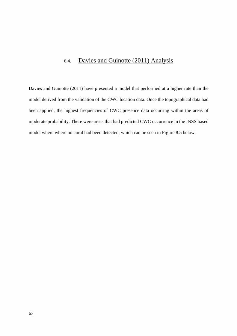
Davies and Guinotte (2011) have presented a model that performed at a higher rate than the
model derived from the validation of the CWC location data. Once the topographical data had
been applied, the highest frequencies of CWC presence data occurring within the areas of
moderate probability. There were areas that had predicted CWC occurrence in the INSS based
model where where no coral had been detected, which can be seen in Figure 8.5 below.

64
Figure 8.5: Dive 10
65
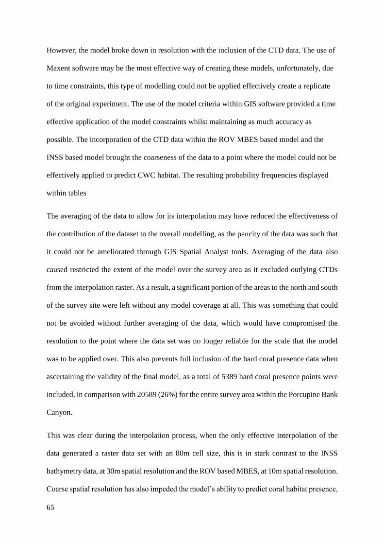
However, the model broke down in resolution with the inclusion of the CTD data. The use of
Maxent software may be the most effective way of creating these models, unfortunately, due
to time constraints, this type of modelling could not be applied effectively create a replicate
of the original experiment. The use of the model criteria within GIS software provided a time
effective application of the model constraints whilst maintaining as much accuracy as
possible. The incorporation of the CTD data within the ROV MBES based model and the
INSS based model brought the coarseness of the data to a point where the model could not be
effectively applied to predict CWC habitat. The resulting probability frequencies displayed
within tables
The averaging of the data to allow for its interpolation may have reduced the effectiveness of
the contribution of the dataset to the overall modelling, as the paucity of the data was such that
it could not be ameliorated through GIS Spatial Analyst tools. Averaging of the data also
caused restricted the extent of the model over the survey area as it excluded outlying CTDs
from the interpolation raster. As a result, a significant portion of the areas to the north and south
of the survey site were left without any model coverage at all. This was something that could
not be avoided without further averaging of the data, which would have compromised the
resolution to the point where the data set was no longer reliable for the scale that the model
was to be applied over. This also prevents full inclusion of the hard coral presence data when
ascertaining the validity of the final model, as a total of 5389 hard coral presence points were
included, in comparison with 20589 (26%) for the entire survey area within the Porcupine Bank
Canyon.
This was clear during the interpolation process, when the only effective interpolation of the
data generated a raster data set with an 80m cell size, this is in stark contrast to the INSS
bathymetry data, at 30m spatial resolution and the ROV based MBES, at 10m spatial resolution.
Coarse spatial resolution has also impeded the model’s ability to predict coral habitat presence,
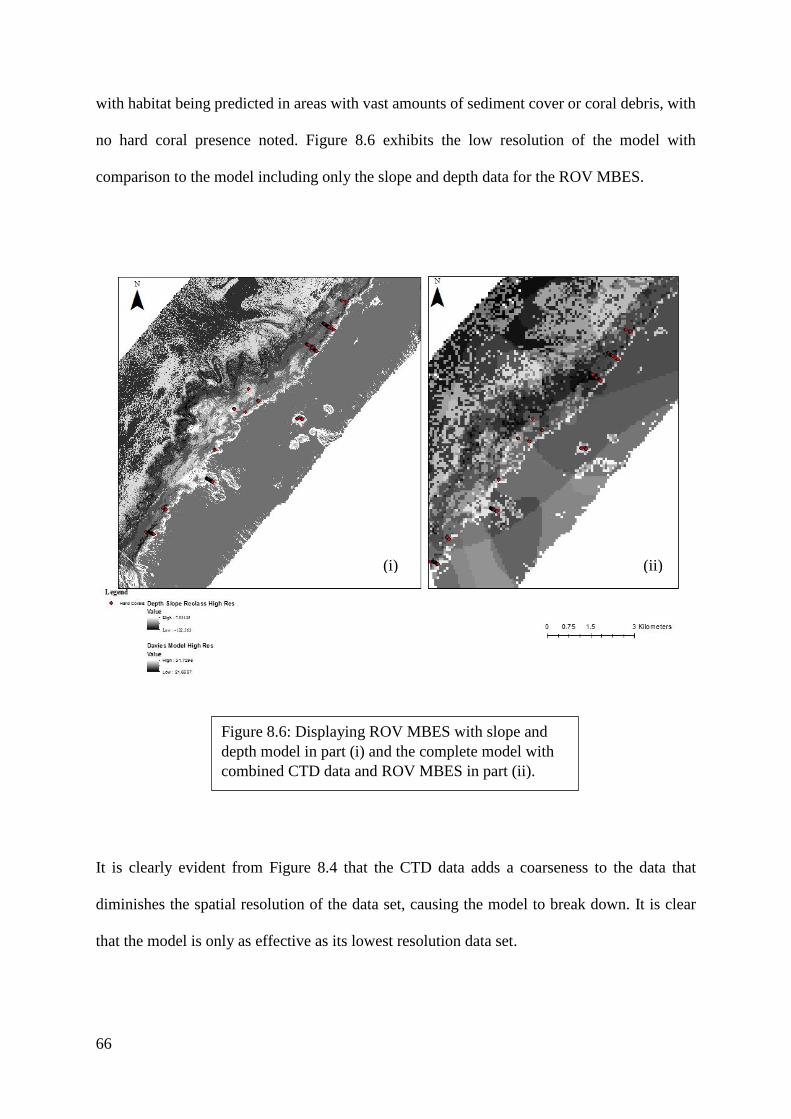
66
with habitat being predicted in areas with vast amounts of sediment cover or coral debris, with
no hard coral presence noted. Figure 8.6 exhibits the low resolution of the model with
comparison to the model including only the slope and depth data for the ROV MBES.
It is clearly evident from Figure 8.4 that the CTD data adds a coarseness to the data that
diminishes the spatial resolution of the data set, causing the model to break down. It is clear
that the model is only as effective as its lowest resolution data set.
Figure 8.6: Displaying ROV MBES with slope and
depth model in part (i) and the complete model with
combined CTD data and ROV MBES in part (ii).
(i) (ii)

67
Due to lack of consistency within the CTD data, effective interpolations of the information
collected could only be made in waters with depths between 1100-0m, as only a quarter of total
dives were below 1100m. This could have been avoided by potentially taking more CTD casts
and increasing the size of the overall dataset to nullify these effects. The clustering of the CTDs
observed in Figure 2.0 open up the data to bias and strong spatial correlation factors may limit
the final dataset, a uniform grid of video lines with regular CTD casts taken may help to
increase the spatial resolution of the data and eliminate any additional spatial biases from
creeping into the data.
Another factor that contributed to the coarseness of the CTD data may have due to the fact that
the original CTD casts were taken at irregular intervals and the resulting dataset had antecedent
inconsistent spatial resolution. This factor is clearly evident when considering the positions of
the CTDs within Habitat Type (1), here the dives are greater in length, with the upcasts and
downcasts occurring at an increased distance away from each other to the north and south of
the survey area. Averaging of the CTDs was required to effectively interpolate the data,
however, the paucity of the data prevented high spatial resolution analysis of the environmental
data. The contrast between the spatial resolution of the combined terrain data (the slope and
depth raster reclass) and the final model incorporating the CTD data underlines the impact that
this paucity has.
The presence data displayed mainly occurred within probabilities of 40-60% within both the
INSS and ROV MBES data models, suggesting that the resolution of MBES data may not have
had a significant impact on the validity of the data as the results were consistent for both
resolutions. The criteria taken from the model created by Davies and Guinotte (2011) for
MBES data may not accurately depict CWC probability at local scales. This can be seen as the
final model for the INSS MBES displays a distribution of 71% of hard corals within the INSS
final model data set were found to occur in zones with a probability of 42% to 63%.

68
6.5. Environmental Parameters
Once the CTD data had been plotted it was quite clear that a significant portion followed a
similar pattern in terms of temperature, density, and dissolved oxygen content with descent
along the water column that had been mentioned previously in the literature as being indicators
of certain water masses (White et al. 2007; Mazzini et al. 2011). Higher temperatures and
salinities observed at depths between 200 to 700m, here temperatures were relatively stable
with little differentiation between the values, this would coincide with the ENAW. A
thermocline occurs at 700m, coinciding with the Mediterranean Ouflow Water (MOW), here
temperatures and salinity begin to fall dramatically as oxygen increases with depth, and closer
to the influence of the Labrador Sea Water (Mienis et al. 2007). The nature of the CTD data
collection truncated the view of the data once they were incorporated into the GIS, as the lack
of depth with many of the upcasts resulted in extreme paucity in waters with a depth of 1100m
or greater. With only 7 CTD casts included in the averaged dataset.
However, due to technical problems CTD data files were corrupted with varying degrees of
severity (partial data had been recovered from CTDs 20, 23, 29, 30, 32, 37, 40, 41, 42 and 45).
Most of the data was recoverable for use in the model, however CTDs 23 & 40 were not
included as the depth values were incorrect for CTD 40 and the file for CTD 23 was corrupted
such that the data after a depth of 123m was beyond use, both files were not included in the
final dataset. CTD 22 was aborted after the ROV had been dispatched as the vessel was in the
wrong area. CTD 31 lacked data for the first 100m, however the rest of the data was recovered.
Due to technical errors the SBE 911 failed to record after the first dive, the CTD for the ROV
Holland was substituted for this for CTDs 40-43, the SBE 911 had been repaired for CTDs 40-

69
43, however the repair had failed after CTD 43. The CTDs show a strong clustering of the CTD
data is seen in towards the centre of the survey area, with the data becoming more sparsely
distributed in over Habitat Type (1), the north and south of the area. CTD coverage within the
Habitat Type (1) totals 17 CTDs, this is in contrast to the remaining 29 CTDs covering the
Habitat Type (2) at the centre of the survey site.
7. Conclusions
It is clear from the evidence below that the model provided by Davies and Guinotte (2011) is
one that requires much more field data to be applied at a local scale resolution. However, with
feasibility restrictions such as the substantial cost of gathering this data as well as the time
required to maintain a reliable database, local scale predictive habitat models may not be
possible with the current technology and extent of knowledge today. As seen throughout the
study, the UNEP CWC database is not an exhaustive list of CWC presence, yet is remains the
most extensive and reliable database for CWCs and is employed within many habitat models.
Such compromises are regularly made within CWC predictive habitat models as they are often
an amalgamation of datasets taken over wide temporal and spatial resolutions in order to
compensate for the paucity of datasets (Davies et al. 2008; Guinotte and Davies 2014; Davies
and Guinotte 2011). Thus, inconsistencies within the data may ultimately create a model that
has applications on global scale, where the coarseness of this data is complements the scale
onto which it is applied.
The marine habitat of the Porcupine Bank Canyon exhibits traits that suggest that its
complexity may not be realised through global scale analysis. A narrower focus on

70
environmental parameters within the survey site coupled with local specific CWC presence
data may be required for finer scale habitat modelling. Terrestrial habitat models have been
well proven or have access to meticulous and reliable data, much of which is open to the public
and can be collected throughout the calendar year on a variety of spatial and spectral
resolutions, enabling the most accurate predictions to be made (Becker et al. 2009). The
accessibility of the field within these environments varies between environments, however
oftentimes, instruments may be left in strategic areas to augment this remote sensing data with
fresh field survey data. Until cost effective methods of deep marine field surveying become
accessible to the wider scientific community the overall resolution of the data extracted from
the deep marine environments of the world will remain at a coarse resolution. With predictive
habitat modelling restricted to producing predictions at small scale resolutions.
8. Acknowledgements
I would like to commend a group of people, who have not only assisted in the execution of this
model, but also amplified its effectiveness and accuracy with their steadfast knowledge and
keen insight into the nature of CWC habitats. Firstly, I would like to thank my supervisor
Professor Andy Wheeler, without whom this model would not exist. I would also like to thank
Dr. Aaron Lim, whose patience and tenacity accelerated the analysis with his wealth of
knowledge on CWC studies and GIS experience. I would like to thank Helen Bradley of the
Geography Department, whose knowledge on GIS and predictive habitat suitability algorithms
assisted in correcting many of the mistakes and blunders generated by the author. Lastly, I

71
would like to thank Saoirse O’Neill, whose constant support and encouragement provided the
fuel to finish the project and to create it to the best possible standard.
9. References
9.1. Books & Papers
Aanesen, M., Armstrong, C., Czajkowski, M., Falk-Petersen, J., Hanley, N. and Navrud, S.
(2015). Willingness to pay for unfamiliar public goods: Preserving cold-water coral in Norway.
Ecological Economics, 112, pp.53-67.
Andrews, A.H., Cordes, E.E., Mahoney, M.M., Munk, K., Coale, K.H., Cailliet, G.M., and
Heifetz, J., (2002). Age, growth and radiometric age validation of a deep-sea, habitat-forming
gorgonian (Primnoa resedaeformis) from the Gulf of Alaska. Hydrobiologia (471), pp.101–
110.
Armstrong, C., Foley, N., Kahui, V. and Grehan, A. (2014). Cold water coral reef management
from an ecosystem service perspective. Marine Policy, 50, pp.126-134.
Armstrong, C., Foley, N., Tinch, R. and van den Hove, S. (2012). Services from the deep: Steps
towards valuation of deep sea goods and services. Ecosystem Services, 2, pp.2-13.
Armstrong, C. and van den Hove, S. (2008). The formation of policy for protection of cold-
water coral off the coast of Norway. Marine Policy, 32(1), pp.66-73.
Arzola, R., Wynn, R., Lastras, G., Masson, D. and Weaver, P. (2008). Sedimentary features
and processes in the Nazaré and Setúbal submarine canyons, west Iberian margin. Marine
Geology, 250(1-2), pp.64-88.

72
Baillon, S., Hamel, J., Wareham, V. and Mercier, A. (2012). Deep cold-water corals as
nurseries for fish larvae. Frontiers in Ecology and the Environment, 10(7), pp.351-356.
Becker, J., Sandwell, D., Smith, W., Braud, J., Binder, B., Depner, J., Fabre, D., Factor, J.,
Ingalls, S., Kim, S., Ladner, R., Marks, K., Nelson, S., Pharaoh, A., Trimmer, R., Von
Rosenberg, J., Wallace, G. and Weatherall, P. (2009). Global Bathymetry and Elevation Data
at 30 Arc Seconds Resolution: SRTM30_PLUS. Marine Geodesy, 32(4), pp.355-371.
Bennett, E., Peterson, G. and Gordon, L. (2009). Understanding relationships among multiple
ecosystem services. Ecology Letters, 12(12), pp.1394-1404.
Bongiorni, L., Mea, M., Gambi, C., Pusceddu, A., Taviani, M. and Danovaro, R. (2010). Deep-
water scleractinian corals promote higher biodiversity in deep-sea meiofaunal assemblages
along continental margins. Biological Conservation, 143(7), pp.1687-1700.
Bouchet, P., 2006 The Magnitude of Marine Biodiversity. In: Duarte, C.M. (Ed.), The
Exploration of Marine Biodiversity, pp. 32-64.
Brown, C., Smith, S., Lawton, P. and Anderson, J. (2011). Benthic habitat mapping: A review
of progress towards improved understanding of the spatial ecology of the seafloor using
acoustic techniques. Estuarine, Coastal and Shelf Science, 92(3), pp.502-520.
Büscher, J., Form, A. and Riebesell, U. (2017). Interactive Effects of Ocean Acidification and
Warming on Growth, Fitness and Survival of the Cold-Water Coral Lophelia pertusa under
Different Food Availabilities. Frontiers in Marine Science, 4.
Cathalot, C., Van Oevelen, D., Cox, T., Kutti, T., Lavaleye, M., Duineveld, G. and Meysman,
F. (2015). Cold-water coral reefs and adjacent sponge grounds: hotspots of benthic respiration
and organic carbon cycling in the deep sea. Frontiers in Marine Science, 2.
73
Clark, M., O’Driscoll, R., (2003). Deepwater fisheries and aspects of their impact on seamount
habitat in New Zealand. Journal of Northwest Atlantic Fishery Science 31, 441–458.
Clark, M. and Rowden, A. (2009). Effect of deepwater trawling on the macro-invertebrate
assemblages of seamounts on the Chatham Rise, New Zealand. Deep Sea Research Part I:
Oceanographic Research Papers, 56(9), pp.1540-1554.
Cordes, E., Arnaud‐Haond, S., Bergstad, O., Da Costa Falcao, A. P., Freiwald, A., Murray
Roberts, L., & Bernal, P. (2016). Cold water corals. United Nations: In The first global
integrated marine assessment. Division for ocean affairs and the law of the sea.
Costello, M., Coll, M., Danovaro, R., Halpin, P., Ojaveer, H. and Miloslavich, P. (2010). A
Census of Marine Biodiversity Knowledge, Resources, and Future Challenges. PLoS ONE,
5(8), p.e12110.
Davies, A. and Guinotte, J. (2011). Global Habitat Suitability for Framework-Forming Cold-
Water Corals. PLoS ONE, 6(4), p.e18483.
Davies, A., Wisshak, M., Orr, J. and Murray Roberts, J. (2008). Predicting suitable habitat for
the cold-water coral Lophelia pertusa (Scleractinia). Deep Sea Research Part I: Oceanographic
Research Papers, 55(8), pp.1048-1062.
De Clippele, L., Gafeira, J., Robert, K., Hennige, S., Lavaleye, M., Duineveld, G., Huvenne,
V. and Roberts, J. (2016). Using novel acoustic and visual mapping tools to predict the small-
scale spatial distribution of live biogenic reef framework in cold-water coral habitats. Coral
Reefs, 36(1), pp.255-268.
De Mol, B., Keppens, E., Swennen, R., Henriet, J. P., (1998). Isotopic characterisation of
ahermatypic coral on a ‘Hovland’ mound. In: De Mol B (ed) Geosphere-biosphere coupling:
carbonate mud mounds and cold-water reefs. International Conference and 6th Post-Cruise

74
Meeting of the Training Through Research Programme, 7–11 February 1998, Gent, Belgium.
Intergovernmental Oceanographic Commission, UNESCO, Worksh Rep 143, pp. 31–32.
D’Onghia, G., Calculli, C., Capezzuto, F., Carlucci, R., Carluccio, A., Grehan, A., Indennidate,
A., Maiorano, P., Mastrototaro, F., Pollice, A., Russo, T., Savini, A., Sion, L. and Tursi, A.
(2016). Anthropogenic impact in the Santa Maria di Leuca cold-water coral province
(Mediterranean Sea): Observations and conservation straits. Deep Sea Research Part II: Topical
Studies in Oceanography.
Dorschel, B. (2011). Atlas of the deep-water seabed. Dordrecht: Springer.
Dullo W, C., Flögel, S. and Rüggeberg, A. (2008). Cold-water coral growth in relation to the
hydrography of the Celtic and Nordic European continental margin. Marine Ecology Progress
Series, 371, pp.165-176.
Fabri, M., Pedel, L., Beuck, L., Galgani, F., Hebbeln, D. and Freiwald, A. (2014). Megafauna
of vulnerable marine ecosystems in French mediterranean submarine canyons: Spatial
distribution and anthropogenic impacts. Deep Sea Research Part II: Topical Studies in
Oceanography, 104, pp.184-207.
Flögel, S., Dullo, W., Pfannkuche, O., Kiriakoulakis, K. and Rüggeberg, A. (2014).
Geochemical and physical constraints for the occurrence of living cold-water corals. Deep Sea
Research Part II: Topical Studies in Oceanography, 99, pp.19-26.
Foley, N., van Rensburg, T. and Armstrong, C. (2010). The ecological and economic value of
cold-water coral ecosystems. Ocean & Coastal Management, 53(7), pp.313-326.
Foubert, A., Huvenne, V., Wheeler, A., Kozachenko, M., Opderbecke, J. and Henriet, J. (2011).
The Moira Mounds, small cold-water coral mounds in the Porcupine Seabight, NE Atlantic:

75
Part B—Evaluating the impact of sediment dynamics through high-resolution ROV-borne
bathymetric mapping. Marine Geology, 282(1-2), pp.65-78.
Frank, N., Freiwald, A., Correa, M., Wienberg, C., Eisele, M., Hebbeln, D., Van Rooij, D.,
Henriet, J., Colin, C., van Weering, T., de Haas, H., Buhl-Mortensen, P., Roberts, J., De Mol,
B., Douville, E., Blamart, D. and Hatte, C. (2011). Northeastern Atlantic cold-water coral reefs
and climate. Geology, 39(8), pp.743-746.
Freiwald, A. and Roberts, J. (2005). Cold-water corals and ecosystems. Berlin: Springer.
Freiwald A, Rogers A, Hall-Spencer J, Guinotte JM, Davies AJ, Yesson C, Martin CS,
Weatherdon LV (2017). Global distribution of cold-water corals (version 3.0). Second update
to the dataset in Freiwald et al. (2004) by UNEP-WCMC, in collaboration with Andre Freiwald
and John Guinotte. Cambridge (UK): UNEP World Conservation Monitoring
Centre. URL: http://data.unep-wcmc.org/datasets/3
García, R., van Oevelen, D., Soetaert, K., Thomsen, L., De Stigter, H. and Epping, E. (2008).
Deposition rates, mixing intensity and organic content in two contrasting submarine canyons.
Progress in Oceanography, 76(2), pp.192-215.
Gass, S. and Roberts, J. (2006). The occurrence of the cold-water coral Lophelia pertusa
(Scleractinia) on oil and gas platforms in the North Sea: Colony growth, recruitment and
environmental controls on distribution. Marine Pollution Bulletin, 52(5), pp.549-559.
Glenn, H., Wattage, P., Mardle, S., Rensburg, T., Grehan, A. and Foley, N. (2010). Marine
protected areas—substantiating their worth. Marine Policy, 34(3), pp.421-430.
Goffredo, S. and Dubinsky, Z. (2016). The Cnidaria, past, present and future. 1st ed.

76
Guinan, J., Grehan, A., Dolan, M. and Brown, C. (2009). Quantifying relationships between
video observations of cold-water coral cover and seafloor features in Rockall Trough, west of
Ireland. Marine Ecology Progress Series, 375, pp.125-138.
Guinotte, J. and Davies, A. (2014). Predicted Deep-Sea Coral Habitat Suitability for the U.S.
West Coast. PLoS ONE, 9(4), p.e93918.
Hansen, E., Gobakken, T., Bollandsås, O., Zaha, E. and Næsset, E. (2015). Modelling
Aboveground Biomass in Dense Tropical Submontane Rainforest Using Airborne Laser
Scanner Data. Remote Sensing, 7(1), pp.788-807.
Harsch, M., Phillips, A., Zhou, Y., Leung, M., Rinnan, D. and Kot, M. (2017). Moving forward:
insights and applications of moving-habitat models for climate change ecology. Journal of
Ecology.
Henry, L., Davies, A. and Murray Roberts, J. (2009). Beta diversity of cold-water coral reef
communities off western Scotland. Coral Reefs, 29(2), pp.427-436.
Hirzel, A., Le Lay, G., Helfer, V., Randin, C. and Guisan, A. (2006). Evaluating the ability of
habitat suitability models to predict species presences. Ecological Modelling, 199(2), pp.142-
152.
Husebø, A, Nottestad, L, Fossa, J, Furevik, D, and Jorgensen, S. (2002). Distribution and
abundance of fish in deep sea coral habitats. Hydrobiologia, 471, pp.91–9.
Huvenne, V., Tyler, P., Masson, D., Fisher, E., Hauton, C., Hühnerbach, V., Le Bas, T. and
Wolff, G. (2011). A Picture on the Wall: Innovative Mapping Reveals Cold-Water Coral
Refuge in Submarine Canyon. PLoS ONE, 6(12), p.e28755.
77
Huvenne, V., Bett, B., Masson, D., Le Bas, T. and Wheeler, A. (2016). Effectiveness of a deep-
sea cold-water coral Marine Protected Area, following eight years of fisheries closure.
Biological Conservation, 200, pp.60-69.
Hübscher, C., Dullo, C., Flögel, S., Titschack, J. and Schönfeld, J. (2010). Contourite drift
evolution and related coral growth in the eastern Gulf of Mexico and its gateways. International
Journal of Earth Sciences, 99(S1), pp.191-206.
Jones, C., Lawton, J. and Shachak, M. (1997). Positive and Negative Effects of Organisms as
Physical Ecosystem Engineers. Ecology, 78(7), p.1946.
Kano, A., Ferdelman, T., Williams, T., Henriet, J., Ishikawa, T., Kawagoe, N., Takashima, C.,
Kakizaki, Y., Abe, K., Sakai, S., Browning, E. and Li, X. (2007). Age constraints on the origin
and growth history of a deep-water coral mound in the northeast Atlantic drilled during
Integrated Ocean Drilling Program Expedition 307. Geology, 35(11), p.1051.
Kenyon, N., Akhmetzhanov, A., Wheeler, A., van Weering, T., de Haas, H. and Ivanov, M.
(2003). Giant carbonate mud mounds in the southern Rockall Trough. Marine Geology, 195(1-
4), pp.5-30.
Kilpatrick, R., Ewing, G., Lamb, T., Welsford, D. and Constable, A. (2011). Autonomous video
camera system for monitoring impacts to benthic habitats from demersal fishing gear, including
longlines. Deep Sea Research Part I: Oceanographic Research Papers, 58(4), pp.486-491.
Lagasse, C., Knudby, A., Curtis, J., Finney, J. and Cox, S. (2015). Spatial analyses reveal
conservation benefits for cold-water corals and sponges from small changes in a trawl fishery
footprint. Marine Ecology Progress Series, 528, pp.161-172.

78
Lambert, C., Mannocci, L., Lehodey, P. and Ridoux, V. (2014). Predicting Cetacean Habitats
from Their Energetic Needs and the Distribution of Their Prey in Two Contrasted Tropical
Regions. PLoS ONE, 9(8), p.e105958.
Larsson, A., van Oevelen, D., Purser, A. and Thomsen, L. (2013). Tolerance to long-term
exposure of suspended benthic sediments and drill cuttings in the cold-water coral Lophelia
pertusa. Marine Pollution Bulletin, 70(1-2), pp.176-188.
Lastras, G., Canals, M., Ballesteros, E., Gili, J. and Sanchez-Vidal, A. (2016). Cold-Water
Corals and Anthropogenic Impacts in La Fonera Submarine Canyon Head, Northwestern
Mediterranean Sea. PLOS ONE, 11(5), p.e0155729.
Lim, A., Wheeler, A. and Arnaubec, A. (2017). High-resolution facies zonation within a cold-
water coral mound: The case of the Piddington Mound, Porcupine Seabight, NE Atlantic.
Marine Geology, 390, pp.120-130.
Lindner, A., Cairns, S. and Cunningham, C. (2008). From Offshore to Onshore: Multiple
Origins of Shallow-Water Corals from Deep-Sea Ancestors. PLoS ONE, 3(6), p.e2429.
Linnaeus, C. (1758). Systema Naturae per regna tria naturae, secundum classes, ordines,
genera, species, cum chararteibus, differentiis, synonymis, locis (Holmiae: Laurentii Salvii),
Stolkhom.
Mazzini, A., Akhmetzhanov, A., Monteys, X. and Ivanov, M. (2011). The Porcupine Bank
Canyon coral mounds: oceanographic and topographic steering of deep-water carbonate mound
development and associated phosphatic deposition. Geo-Marine Letters, 32(3), pp.205-225.3.
McNyset, K. (2005). Use of ecological niche modelling to predict distributions of freshwater
fish species in Kansas. Ecology of Freshwater Fish, 14(3), pp.243-255.

79
Mienis, F., de Stigter, H., White, M., Duineveld, G., de Haas, H. and van Weering, T. (2007).
Hydrodynamic controls on cold-water coral growth and carbonate-mound development at the
SW and SE Rockall Trough Margin, NE Atlantic Ocean. Deep Sea Research Part I:
Oceanographic Research Papers, 54(9), pp.1655-1674.
Mikkelsen, N., Erlenkeuser, H., Killingley, J. and Berger, W. (2008). Norwegian corals:
radiocarbon and stable isotopes in Lophelia pertusa. Boreas, 11(2), pp.163-171.
Miller, R., Hocevar, J., Stone, R. and Fedorov, D. (2012). Structure-Forming Corals and
Sponges and Their Use as Fish Habitat in Bering Sea Submarine Canyons. PLoS ONE, 7(3),
p.e33885.
Morris, K., Tyler, P., Masson, D., Huvenne, V. and Rogers, A. (2013). Distribution of cold-
water corals in the Whittard Canyon, NE Atlantic Ocean. Deep Sea Research Part II: Topical
Studies in Oceanography, 92, pp.136-144.
Mortensen, P., Rapp, H. and Båmstedt, U. (1998). Oxygen and carbon isotope ratios related to
growth line patterns in skeletons of Lophelia pertusa (L) (Anthozoa, Scleractinia): Implications
for determination of linear extension rate. Sarsia, 83(5), pp.433-446.
Mullineaux LS, Mills SW. Coral Gardens in the Dark Depths Oceanus, 2005. p. 22 – 27.
Navas, J., Miller, P., Henry, L., Hennige, S. and Roberts, J. (2014). Ecohydrodynamics of Cold-
Water Coral Reefs: A Case Study of the Mingulay Reef Complex (Western Scotland). PLoS
ONE, 9(5), p.e98218.
New, A. and Smythe-Wright, D. (2001). Aspects of the circulation in the Rockall Trough.
Continental Shelf Research, 21(8-10), pp.777-810.
NPWS., (2016). Conservation objectives for Porcupine Bank Canyon SAC [003001]. Generic
Version 5.0. Department of Arts, Heritage, Regional, Rural and Gaeltacht Affairs.

80
Oevelen, D., Duineveld, G., Lavaleye, M., Mienis, F., Soetaert, K. and Heip, C. (2009). The
cold-water coral community as hotspot of carbon cycling on continental margins: A food-web
analysis from Rockall Bank (northeast Atlantic). Limnology and Oceanography, 54(6),
pp.1829-1844.
Peterson, A. (2001). Predicting species’ geographic distributions based on ecological niche
modelling. The Condor, 103(3), p.599.
Pollard, R., Grifftths, M., Cunningham, S., Read, J., Pérez, F. and Ríos, A. (1996). Vivaldi
1991 - A study of the formation, circulation and ventilation of Eastern North Atlantic Central
Water. Progress in Oceanography, 37(2), pp.167-192.
Przeslawski, R., Currie, D., Sorokin, S., Ward, T., Althaus, F. and Williams, A. (2011). Utility
of a spatial habitat classification system as a surrogate of marine benthic community structure
for the Australian margin. ICES Journal of Marine Science, 68(9), pp.1954-1962.
Quaresma, L., Vitorino, J., Oliveira, A. and da Silva, J. (2007). Evidence of sediment
resuspension by nonlinear internal waves on the western Portuguese mid-shelf. Marine
Geology, 246(2-4), pp.123-143.
Roberts, J. and Cairns, S. (2014). Cold-water corals in a changing ocean. Current Opinion in
Environmental Sustainability, 7, pp.118-126.
Robert, K., Jones, D., Roberts, J. and Huvenne, V. (2016). Improving predictive mapping of
deep-water habitats: Considering multiple model outputs and ensemble techniques. Deep Sea
Research Part I: Oceanographic Research Papers, 113, pp.80-89.
Roberts, J. (2005). Reef-aggregating behaviour by symbiotic eunicid polychaetes from cold-
water corals: do worms assemble reefs?. Journal of the Marine Biological Association of the
United Kingdom, 85(4), pp.813-819.

81
Roberts, J., Wheeler, A. and Freiwald, A. (2006). Reefs of the Deep: The Biology and Geology
of Cold-Water Coral Ecosystems. Science, 312(5773), pp.543-547.
Rogers, A. (1999). The Biology of Lophelia pertusa (Linnaeus1758) and Other Deep-Water
Reef-Forming Corals and Impacts from Human Activities. International Review of
Hydrobiology, 84(4), pp.315-406.
Ross, R. and Howell, K. (2012). Use of predictive habitat modelling to assess the distribution
and extent of the current protection of ‘listed’ deep-sea habitats. Diversity and Distributions,
19(4), pp.433-445.
Rossi, S., Bramanti, L., Gori, A. and Orejas Saco del Valle, C. (2017.). Marine animal forests.
Sampaio, Í., Braga-Henriques, A., Pham, C., Ocaña, O., de Matos, V., Morato, T. and Porteiro,
F. (2012). Cold-water corals landed by bottom longline fisheries in the Azores (north-eastern
Atlantic). Journal of the Marine Biological Association of the United Kingdom, 92(07),
pp.1547-1555.
Sandwell, D., Smith, W., Gille, S., Kappel, E., Jayne, S., Soofi, K., Coakley, B. and Géli, L.
(2006). Bathymetry from space: Rationale and requirements for a new, high-resolution
altimetric mission. Comptes Rendus Geoscience, 338(14-15), pp.1049-1062.
Sheppard, C. (2013). Coral reefs of the United Kingdom Overseas Territories. Dordrecht:
Springer.
Stillman, R., Wood, K. and Goss-Custard, J. (2016). Deriving simple predictions from complex
models to support environmental decision-making. Ecological Modelling, 326, pp.134-141.
Thiem, Ø., Ravagnan, E., Fosså, J. and Berntsen, J. (2006). Food supply mechanisms for cold-
water corals along a continental shelf edge. Journal of Marine Systems, 60(3-4), pp.207-219.

82
Tittensor, D., Baco, A., Hall-Spencer, J., Orr, J. and Rogers, A. (2010). Seamounts as refugia
from ocean acidification for cold-water stony corals. Marine Ecology, 31, pp.212-225.
Van Rooij, D. (2004). An integrated study of Quaternary sedimentary processes on the eastern
slope of the Porcupine Seabight, SW of Ireland, Universiteit Gent. Unpublised phD thesis, pp
1-330.
Vetter, E., Smith, C. and De Leo, F. (2010). Hawaiian hotspots: enhanced megafaunal
abundance and diversity in submarine canyons on the oceanic islands of Hawaii. Marine
Ecology, 31(1), pp.183-199.
Wagner, D., Luck, D.G., Toonen, R.J., (2012). Chapter two-the biology and ecology of black
corals (Cnidaria: Anthozoa: Hexacorallia: Antipatharia). Adv. Mar. Biol. 63, pp.67–132.
Wheeler, A. J., Capocci, R., Crippa, L., Connolly, N., Hogan, R., Lim, A., McCarthy, E.,
McGonigle, C., O’Donnell, E., O’Sullivan, K., Power, K., Ryan, G., Vertino, A., (2015).
Holland 1 ROV technical team, Officers and crew of the RV Celtic Explorer. In: Cruise Report:
Quantifying Environmental Controls on Coldwater Coral Reef Growth (QuERCI). University
College Cork, Ireland.
Wheeler, A.J., Capocci, R., Crippa, L., Connolly, N., Hogan, R., Lim, A., McCarthy, E.,
McGonigle, C., O'Donnell, E., O'Sullivan, K., Power, K., Ryan, G., Vertino, A., 2015. Holland
1 ROV technical team, officers and crew of the RV celtic explorer. In: Cruise Report:
Quantifying Environmental Controls on Cold-Water Coral Reef Growth (QuERCi). University
College Cork, Ireland.
Wheeler, A., Kozachenko, M., Henry, L., Foubert, A., de Haas, H., Huvenne, V., Masson, D.
and Olu, K. (2011). The Moira Mounds, small cold-water coral banks in the Porcupine
Seabight, NE Atlantic: Part A—an early stage growth phase for future coral carbonate
mounds?. Marine Geology, 282(1-2), pp.53-64.

83
White, M. and Dorschel, B. (2010). The importance of the permanent thermocline to the cold
water coral carbonate mound distribution in the NE Atlantic. Earth and Planetary Science
Letters, 296(3-4), pp.395-402.
White HK, Hsing P-Y, Cho W, Shank TM, Cordes EE, Quattrini AM, Nelson RK, and Camilli
R, (2012). emopoulos AWJ, German CR et al.: Impact of the Deepwater Horizon oil spill on a
deep-water coral community in the Gulf of Mexico. Proc Natl Acad Sci U S A 2012, (109)
pp.20303-20308.
White, M., Mohn, C., de Stigter, H.C., Mottram, G., (2005). Deep-water coral development as
a function of hydrodynamics and surface productivity around the submarine banks of the
Rockall Trough, NE Atlantic. In: Freiwald, A., Roberts, J.M. (Eds.), Cold-water Corals and
Ecosystems. In Springer, Berlin, Heidelberg, New York, pp. 503–514.
White, M., Roberts, J. and van Weering, T. (2007). Do bottom-intensified diurnal tidal currents
shape the alignment of carbonate mounds in the NE Atlantic?. Geo-Marine Letters, 27(6),
pp.391-397.
Yesson, C., Bedford, F., Rogers, A. and Taylor, M. (2015). The global distribution of deep-
water Antipatharia habitat. Deep Sea Research Part II: Topical Studies in Oceanography.
Zhao, C., Nan, Z., Cheng, G., Zhang, J. and Feng, Z. (2006). GIS-assisted modelling of the
spatial distribution of Qinghai spruce (Picea crassifolia) in the Qilian Mountains, northwestern
China based on biophysical parameters. Ecological Modelling, 191(3-4), pp.487-500.
Zheng, M. and Cao, L. (2014). Simulation of global ocean acidification and chemical habitats
of shallow- and cold-water coral reefs. Advances in Climate Change Research, 5(4), pp.189-
196.

84
Øvrebø, L., Haughton, P. and Shannon, P. (2006). A record of fluctuating bottom currents on
the slopes west of the Porcupine Bank, offshore Ireland — implications for Late Quaternary
climate forcing. Marine Geology, 225(1-4), pp.279-309.
9.2. Websites
Marine.ie. (2017). Marine Institute - Real Map Of Ireland. [online] Available at:
https://www.marine.ie/Home/sites/default/files/MIFiles/Images/IrelandsMarineResources/Th
e%20Real%20Map%20of%20Ireland.jpg [Accessed 21 Sep. 2017].
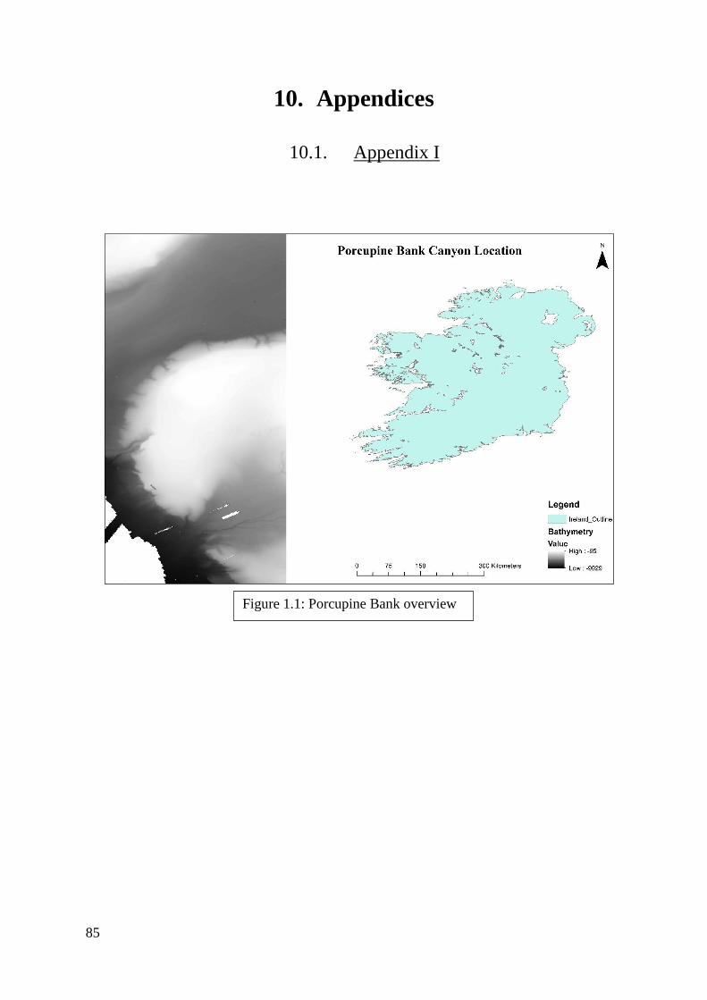
85
10. Appendices
10.1. Appendix I
Figure 1.1: Porcupine Bank overview

86
Figure 1.8: Total ROV dive transects

87
Figure 2.0 CTD locations

88
10.2. Appendix II
Hard Coral Oxygen Frequency
Class Distribution % Frequency Weight
6.011261 0 0 1
6.056792 280 1.449950805 1
6.102322 62 0.321060535 1
6.147852 1049 5.432137124 2
6.193382 3057 15.83035576 6
6.262235 1989 10.29982911 4
6.300497 0 0 0
6.338759 1652 8.554709751 3
6.377022 3438 17.80332453 6
6.415284 1347 6.975299052 2
6.497307 0 0 1
6.541527 0 0 1
6.585747 0 0 1
6.629967 2777 14.38040495 6
6.681546 3660 18.95292838 8
Table 1.1: Frequency Analysis for Hard
Corals with regards Oxygen

89
Hard Coral Depth Frequency INSS
Class Frequency %Total Classification factor
500 to 600 90 0.437126621 1
600 to 700 5729 27.82553791 6
700 to 800 7524 36.54378552 8
800 to 900 4311 20.93836515 5
900 to 1000 2416 11.73442129 2
1000 to 1100 519 2.520763514 1
1100 to 1200 0 0 0
Hard Coral Slope Frequency INSS
Class Frequency % of Total Classification Factor
0 to 10 5365 26.0576 6
10 to 20 7443 36.15037 8
20 to 30 5400 26.2276 6
30 to 40 1261 6.12463 2
40 to 50 1079 5.240662 2
50 to 60 41 0.199135 1
Table 1.2: Hard Coral Presence Data Depth Frequency
INSS Bathymetry Data
Table 1.3: Hard Coral Slope Frequency Data Frequency
INSS Slope Data

90
Hard Coral Salinity
Class Distribution
%
Frequency Weight
34.178791 267 1.3826317 1
34.303 0 0 1
34.434178 0 0 1
34.689565 0 0 1
34.944952 0 0 1
35.086079 0 0 1
35.148529 13 0.0673191 1
35.210979 0 0 1
35.27343 6317 32.711926 3
35.33588 1289 6.6749521 1
35.419441 11425 59.163171 6
Table 1.4 Hard Coral Salinity Frequency

91
Depth Range (m) Weight
2252 2050.55555 6
2050.5555 1849.1111 1
1849.1111 1647.666667 1
1647.6666 1446.222222 1
1446.2222 1244.777778 2
1244.7777 1043.333333 4
1043.3333 841.888889 6
841.88888 640.4444 6
640.44444 439 4
Table 1.5 CWC Depth Weight Classes
(Davies and Guinotte 2011)

92
Slope Range (Radians) Weight
0 0.164159 4
0.164159 0.328319 8
0.328319 0.492478 6
0.492478 0.656638 4
0.656638 0.820797 4
0.820797 0.984957 3
0.984957 1.149116 2
1.149116 1.313276 2
1.313276 1.477435 1
Table 1.6 CWC Slope Weight Classes
(Davies and Guinotte 2011)

93
10.3 Appendix III
Figure 2.2: CTD 2 water column data winch CTD downcast

94
Figure 2.3: CTD 3 water column data upcast

95
Figure 2.4: CTD 4 water column data downcast

96
Figure 2.5: CTD 5 water column data upcast

97
Figure 2.6: CTD 6 water column data downcast

98
Figure 2.7: CTD 7 water column data upcast

99
Figure 2.8: CTD 8 water column data downcast

100
Figure 2.9: CTD 9 water column data upcast
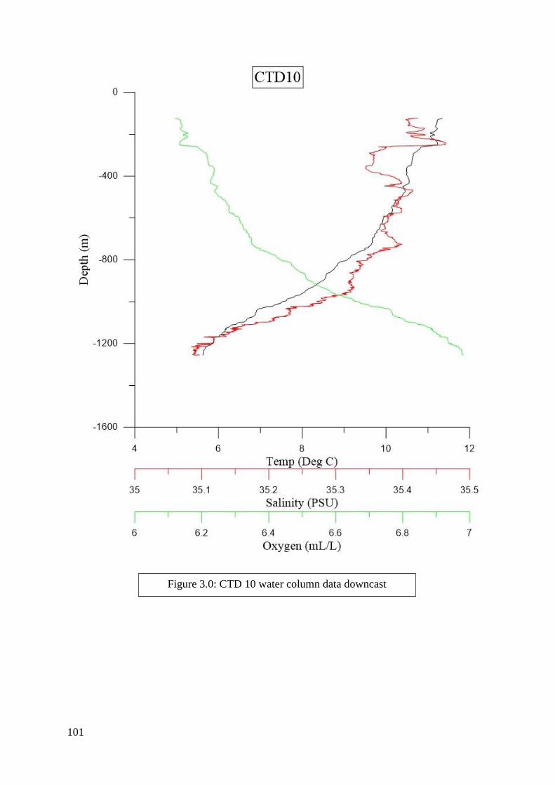
101
Figure 3.0: CTD 10 water column data downcast
Data
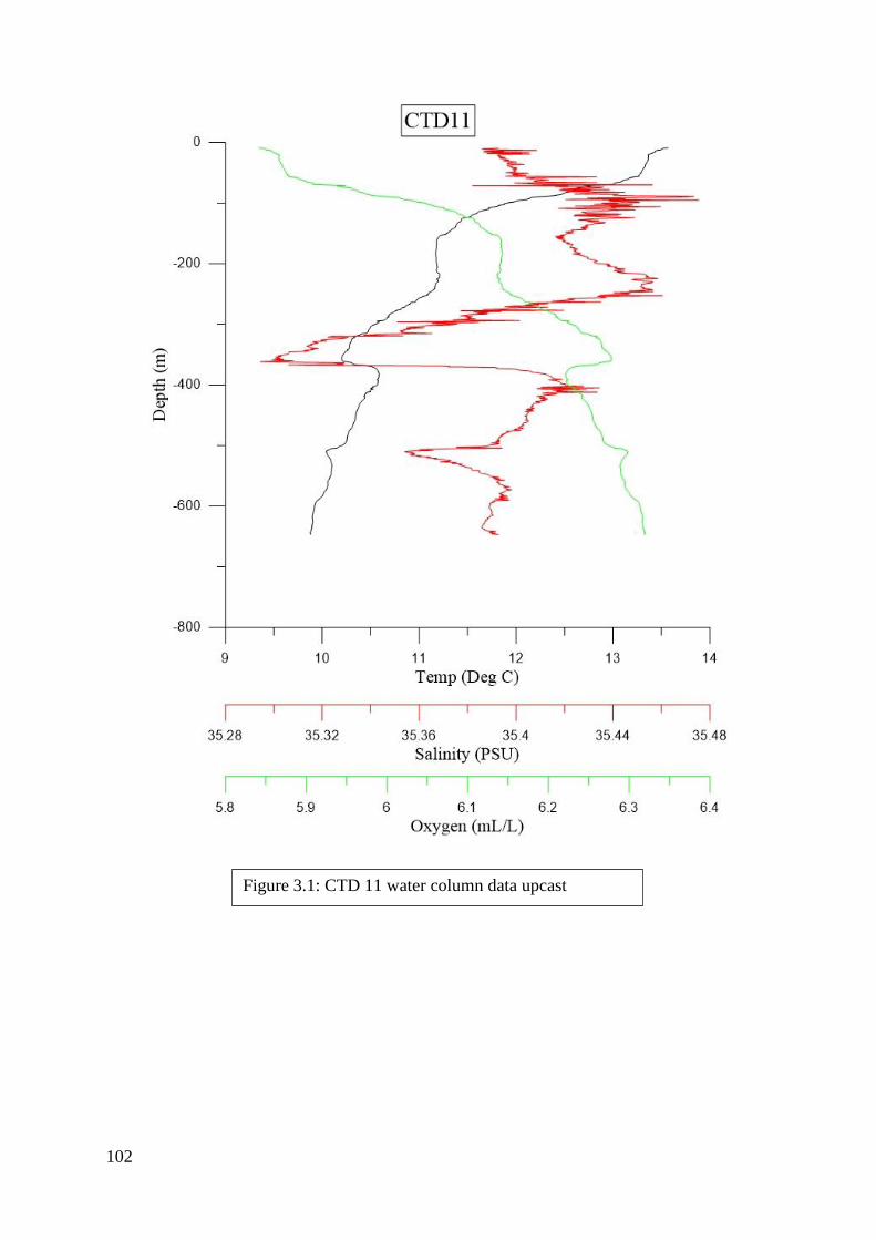
102
Figure 3.1: CTD 11 water column data upcast

103
Figure 3.2: CTD 12 water column data downcast

104
Figure 3.3: CTD 13 water column data upcast

105
Figure 3.4: CTD 14 water column data downcast

106
Figure 3.5: CTD 15 water column data upcast

107
Figure 3.6: CTD 16 water column data downcast
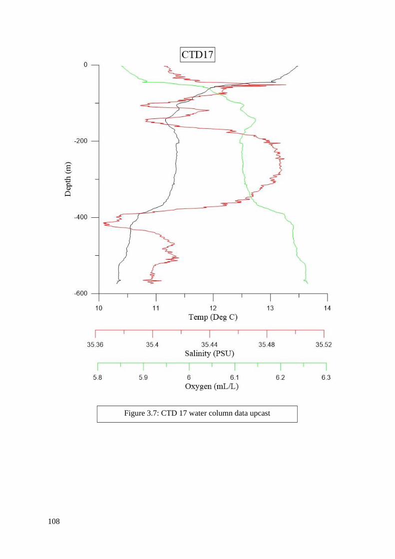
108
Figure 3.7: CTD 17 water column data upcast

109
Figure 3.8: CTD 18 water column data downcast
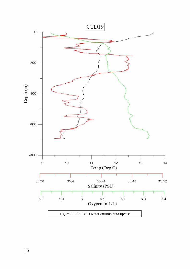
110
Figure 3.9: CTD 19 water column data upcast

111
Figure 4.0: CTD 20 water column data Downcast

112
Figure 4.1: CTD 21 water column data upcast
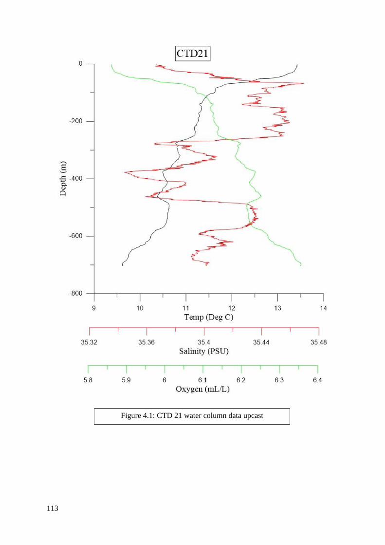
113
Figure 4.1: CTD 21 water column data upcast

114
Figure 4.2: CTD 22 water column data downcast

115
Figure 4.4: CTD 24 water column data upcast

116
Figure 4.5: CTD 25 water column data downcast

117
Figure 4.6: CTD 26 water column data upcast

118
Figure 4.7: CTD 27 water column data downcast

119
Figure 4.8: CTD 28 water column data upcast

120
Figure 4.9: CTD 29 water column data downcast

121
Figure 5.0: CTD 30 water column data upcast
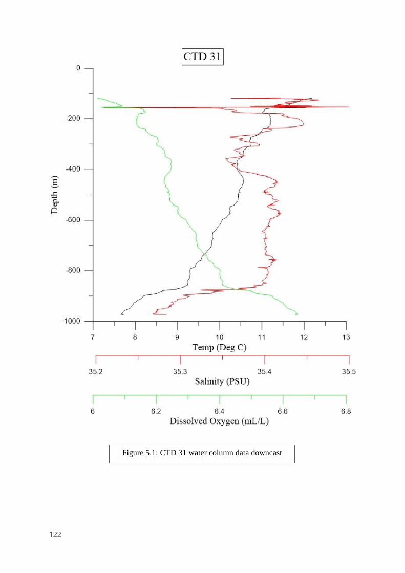
122
Figure 5.1: CTD 31 water column data downcast
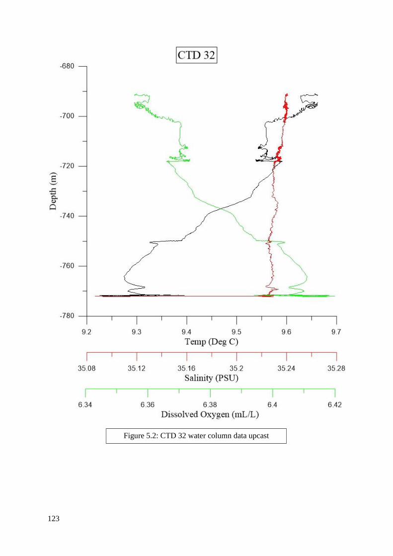
123
Figure 5.2: CTD 32 water column data upcast

124
Figure 5.3: CTD 33 water column data downcast

125
Figure 5.4: CTD 34 water column data upcast

126
Figure 5.5: CTD 35 water column data upcast

127
Figure 5.6: CTD 36 water column data downcast

128
Figure 5.7: CTD 37 water column data upcast

129
Figure 5.8: CTD 38 water column data downcast

130
Figure 5.9: CTD 39 water column data upcast.

131
Figure 6.0: CTD 41 water column data upcast.

132
Figure 6.1: CTD 42 water column data downcast

133
Figure 6.2: CTD 43 water column data upcast

134
Figure 6.3: CTD 44 water column data downcast

135
Figure 6.4: CTD 45 water column data upcast

136
Figure 6.5: CTD 46 water column data downcast

137
Figure 6.6: CTD 47 water column data upcast

138
Figure 6.7: CTD 48 water column data downcast

139
Figure 6.8: CTD 49 water column data downcast

140
10.4 Appendix IV
Figure 7.8: Model from INSS Data

141
Figure 7.9: ROV MBES final model

142

143
Fig 8.1: Dives 10-12, occurring North to South, plotted over INSS
Bathymetry Data. Dive 10 Displays clear lack of coral presence
within zones previously designated by UNEP as confirmed coral
habitat. Dive 11 shows moderate CWC presence however there is a
marked amount of coral debris and sediment facies cover. Dive 12
shows strong CWC presence. (LCF is marked in yellow, sediment
facies is marked in black).

144