Assessing Change in Attitudes, Awareness, and Behavior in Indonesian Youths
Assessing the Impact of Derived Behavior Information on Customer
Attrition in the Financial Service Industry
Abstract
The value of the customer has been widely recognised in terms of financial planning and
efficient resource allocation including the financial service industry. Previous studies have
shown that directly observable information can be used in order to make reasonable
predictions of customer attrition probabilities. However, these studies do not take full account
of customer behavior information. In this paper, we demonstrate that efficient use of
information can add value to financial services industry and improve the prediction of
customer attrition. To achieve this, we apply an orthogonal polynomial approximation
analysis to derive unobservable information, which is then used as explanatory variables in a
probit-hazard rate model. Our results show that derived information can help our
understanding of customer attrition behavior and give better predictions. We conclude that
both researchers and the financial service industry should use derived financial information in
addition to directly observable information.
Key words
Customer attrition; Derived behavior information; Orthogonal polynomial approximation;
Predition; Probit-hazard model.

1. Introduction
Increased competition in the financial service industry has meant that the retention of
existing customers has significantly become more important, especially due to the potential
impact on revenues. Customer retention has also been increasingly of interest to academic
researchers especially in areas of risk assessment and customer behavior, including customer
attrition and attraction (Ganesh et al. 2000; Glady et al. 2008). Financial service firms that
lose existing customers and have to seek new customers incur more expense than those that
retain their customers, not to mention the associated risks involved in taking on new
customers (Verbeke et al. 2012). Studies have shown that various sources of information can
be used for monitoring financial customer behavior in order to facilitate customer-centric
processes (Lessmann and Vob 2009). Dekimpe and Degraeve (1997) identify that customer
demographics are associated with attrition behaviour. Athanassopoulos (2000) and Buckinx
and Van den Poel (2005) provide evidence that product-specific features have significant
impacts on customer attrition. In addition to studying the impact of customer demographic
and product-specific features, Van den Poel and Lariviere (2004) also investigate customer
attrition behaviour changes under different macroeconomic environment. Bose and Chen
(2009) provide an excellent review on types of data used in quantitative models for
customers’ behaviour research.
Thomas (2010) draws attention to many of the challenges for research in customer
behaviour finance, including a lack of focus and integration of marketing information on the
behavior of financial customers. Chen et al (2012) further point out that customer behaviour
is dynamic and the relation evolves overtime. As a result, an essential part of customer
relation should be based on customer lifetime value. However, these studies generally attempt
to use directly observable information to identify and explain customer attrition behavior.
They do not consider the importance of derived information that can help the financial

service industry understand and predict customers’ attrition behavior in a variety of other
ways. Blochlinger and Leippold (2006) show that informationally privileged financial
services firms have competitive advantages over other financial firms.
Based on a classical orthogonal polynomial approximation approach, this paper
derives indirectly observable information from a unique panel dataset, which records the
value of the financial policy holdings history for each customer on a monthly basis. We
simultaneously consider the customer attrition process and the customer relations established
during the initial process of setting up the financial policy. This broader approach allows us
to examine the relations between the two processes and accommodate unobservable
heterogeneity. The derived information can provide financial firms with special insights for
understanding customer attrition behavior. To our knowledge this paper is the first to
examine whether derived information can be exploited by systematically analyzing customer
financial behavior. It shifts the focus of the issue from one using directly observable
information to one in which derived information can also provide valuable information for
the estimation and prediction. This shift is in accord with the study of customer behavior,
where behavioral factors affect the probability of customer attrition.
The results show that, in addition to directly observable information, the derived
information can explain customer attrition behavior and detect triggers for attrition. Both of
these sources of information form essential elements in understanding customer behavioral
attrition with financial firms. The findings of this study further point to the benefits of
incorporating derived information to improve the precision of customer attrition prediction.
Specifically, the explanatory variables derivable from fluctuations in the value of the
financial policy holding can contribute to the attrition probability prediction. One possible
explanation for this is that after customers initially set up relations with a financial firm, their
attrition behaviour is dynamic and subject to many ongoing factors, such as the external

economic environment or various personal reasons. Personal reasons can motivate customers
to change the value of their financial policy holdings. Such changes could provide useful
information for financial firms to infer customers’ attrition behavior. Financial service firms
seeking to use relevant information more efficiently will therefore find the results interesting.
The empirical results also suggest significant correlation between financial policy purchasing
and attrition processes.
The rest of the paper is as follows. In Section 2 we discuss the research questions.
Section 3 presents the data description and the variables used to estimate the model. This
section demonstrates the method of deriving certain factors used as explanatory variables in
the model. Section 4 outlines the specification and estimation of the probit-continuous hazard
multi-process model. Section 5 presents the empirical results and a discussion of these
findings. Section 6 provides the overall model fit tests and the comparison of predictive
power of the models with and without the derived information. Section 7 presents concluding
remarks and the implications of the findings.
2. Research questions
The general question to be addressed in this study is to investigate the relation
between various factors and customer attrition and, in particular, whether or not derived
information can explain customer attrition behaviour. Our first set of hypotheses are based
on Van den Poel and Lariviere (2004) who suggest customer demographics can have impacts
on customer attrition. For example the empirical evidence on whether or not there is a
difference between male and female customers attrition behaviour is mixed. Both Mittal and
Kamakura (2001) and Van den Poel and Lariviere (2004) suggest male customers tend to
have higher attrition rate than female customers. On the other hand Dekimpe and Degraere
(1997) find women are more likely to quit than men. Other research tends to suggest that

older (married) customers are less likely to leave the firm than younger (unmarried) ones..
Finally, Mittal and Kakura (2001) and Van den Poel and Lariviere (2004) examine whether
social status and country of origin have an impact on customer attrition. The results are
mixed.
Based on this previous empirical evidence we formalize our investigation of the
impact of customer demographics on attrition in the following hypotheses:
Hypothesis 1a: There is a positive relation between male customer and attrition behaviour.
Hypothesis 1b: There is a negative relation between customer age and attrition behaviour.
Hypothesis 1c: There is a negative relation between the customer marital status and
attrition behaviour.
Hypothesis 1d: There is a relation between customer financial status and attrition
behaviour.
Hypothesis 1e: There is a relation between customer country origin and attrition behaviour.
Our second hypothesis also follow those proposed by Van den Poel and Lariviere
(2004) as we consider the impact of macroeconomic conditions, including UK stock market
performance, house market performance, interest rate, and customer confidence on customer
attrition. Prior research has shown that the conditions of external economic environment can
have strong and statistically significant effects on customer financial decisions. Van den Poel
and Lariviere (2004) point out that customers experience more switching tendencies in a
favorable macro-economic environment. Thomas et al. (2005) find that customers are more
likely to purchase financial policy products with the rise of stock market and housing market.
Tang et al. (2007) further show that external economic environment can significantly impact
customers’ subsequent financial policy product purchase behaviours. Following this evidence
we expect that the macroeconomic variables can influence the aspect of customer attrition
behaviour.

Hypothesis 2: There is a relation between customer attrition behaviour with macroeconomic
conditions.
Our third hypothesis is our main contribution to the literature as it investigates the
effects of derived information about customer financial policy values on customers’ attrition
behaviour. Derived information is created though the approach of orthogonal polynomial
approximation (see section 3.2 for details). Though the impact of derived information has
rarely been investigated in previous customer attrition literature, we feel that such derived
information can be related to customer perception variables. Van den Poel and Lariviere
(2004) provide an excellent review on the impact of customer perception predictors on
attrition such as company versus competitors performance, customer overall satisfaction
(Keaveney 1995; Bolton et al. 2000) and service quality (Athanassopoulos, 2000). These
empirical studies find a significant decline in customer attrition for firms with better
performance and service quality. Thus we expect that financial firms delivering higher values
for financial policies will tend to reduce the likelihood of customer attrition.
Hypothesis 3: There is a relation between customer attrition behaviour with derived
information based on the value of financial policies.
3. Data and specification of derived variables
3.1 Data description
This section describes the data and the relevant social-demographic and
macroeconomic variables used in our study.. Collection of the data need for this type of study
is difficult and this study was only possible as a major financial insurance company in Great
Britain provided the data, as long as it remained anonymous. The data consists of 19,774
customers who purchase 20,257 financial policies over the 36 months period, from April
2001 through March 2004 (an average of 1.02 financial policies with a standard derivation of
0.17). Of the 19,774 customers, the vast majority (19,321) customers hold single policies.

The rest hold multiple policies and the highest number of policies is 5. Customers register
with the firm at various times, i.e., not all customers have all 36 months of records available.
For each customer, the data record provides observable information on the social-
demographic background: gender, age, marital status, financial status, region, type of
financial policy, and payment frequency. All of the policies provide the policy start date and
the policy end date. Profiles of the 19,774 customers in the data set are as follows: 54.3% are
male; 6.9% customers are under 20, the 20-35 years old customer account for 18.8%, 36%
customers are in the 35-to-55 age group, the rest are those customers aged over 55 and the
mean age of the customers is 48; 15.1% are married; 37.5% have high financial status
(financial A category), 37.6% have intermediate financial status (financial B category), and
the rest have low financial status (financial C or beyond category); 74.2% of the customers
live in England, 17.9% live in Scotland, and the rest live in Ireland. Customers can purchase
three kinds of financial policy. The first policy group consists of collective investment
policies, such as unit trusts (i.e., mutual funds) and individual saving accounts (ISAs). The
second group consists of life insurance policies and the final group consists of pension
policies, such as personal pensions and stakeholder pensions.
Table 1 here
Table 1 shows the number of policy changes over the 36 months period. Of all
20,257 purchased policies, 16,578 (82%) consists of collective investment policies and the
rest are life insurance and protection policies. This study differentiates two main groups: an
investment policy group and a non-investment policy group. One would expect a difference
between investment and non-investment products as investment products the returns are
directly linked to the value of the assets, thus carrying risks. Customers can withdraw the
cash value of the units, subject to possible surrender charges. Early termination of the policy
may be costly and the cash value payable may be less than the total premiums paid. Non-

investment products like insurance are often renewed on an annual basis and so there are
regular opportunities for the customer to churn to another company. The returns from non-
investment products will not necessarily track the ups and downs of investment markets. A
part of the cash values under a participating non-investment policy will be guaranteed Within
the three years customers terminate (churn) a total of 10,050 policies, and continue
with10,207 policies. Over 90% (9,180/10,050) of the churned policies consist of investment
related policies. These figures show that large numbers of customers fail to continue with
their investment policies. Since all customers in the sample set up the relation with the
financial insurance company after April 2001 and we know what the start date for each
customer is, we do not need to deal with the issue of left censoring where the attrition event
occurred before April 2001.
Figure 1 here
Figure 1 displays the empirical product-limit estimator (also known as Kaplan-Meier
estimator) for estimating survival function describing survival distributions curve in our
sample. The horizontal axis shows the duration time and vertical axis gives the survival
probabilities for each time period. The Kaplan-Meier estimate probability shows that a
customer will survive with the insurance company for 5 months or more is 0.909. It declines
to 0.705 and 0.602 for 20 months and 30 months or more, respectively. The median duration
for the policies that continue with the insurance company is 34 months (median is the
preferred measure of central tendency for censored survival data). There are 10,112
customers with 10,201 policies still remaining with the firm (i.e. right censored) at the end of
data period. Accordingly, 9,739 customers terminate 10,050 policies during the three-year
sample period.
The data provided by the UK financial insurance company also records the value (in
UK sterling) of financial policy holding changes for every customer each month, depending

on the duration of the customer’s policy. The value of financial policy holdings used in the
analysis represents the true movements in customer holdings as the effects of the stock
market have been stripped out. In doing so, the value of policy holdings reflects the true
customers’ attrition to the financial insurance firm. The records consist of a sequence of times
and holding values {(t(1),u(1)), . . ., (t(n k ),u(n k ))} for customer k. The length of the
sequence n k varies from customer to customer, depending on the duration with the firm. The
value of holdings is a function of time, piecewise constant with jumps where the holdings
change. In line with Thomas et al. (2005) and Tang et al. (2007), the analysis also includes
four external macroeconomic variables, since attrition decisions made by customers can be
influenced by exogenous economic environmental conditions. Here the chosen variables
reflect the attractiveness of the general economic climate. The external UK economic
variables are the Customer Confidence Index, the House Price Index, the FTSE All Share
Index, and the Bank of England Base Interest Rate. The Augmented Dickey-Fuller unit root
test shows that these economic variables except for Customer Confidence Index are non-
stationary. Therefore those non-stationary variables are transformed by taking the first
difference of the natural logarithm. Table 2 presents all of the variables used in the analysis.
Table 2 here
3.2 Derived variables through orthogonal polynomial approximations
The entire dataset contains detailed information of the financial policy holding value
movements for each month for each customer. To derive information from the monthly
financial policy holding values requires a consistent parameterization of the holding curve for
each customer. Since the policy holding curve reflects the value of holdings held by the
customer over the entire period of the data, this will indicate whether and when the customer
left the firm. Therefore, this analysis does not use the full time series of the customer’s

holding values to derive further information and then predict when the customer owns zero
values, but only uses the holding values from period 1 to 1kn for customer k.
This paper uses an orthogonal polynomial approximation of order 3, in which each
order component, zi, measures the level final holding value, the linear trend, the quadratic
curvature, and change in curvature, i.e. cubic component, respectively. The orthogonal
polynomial approximation makes the size of each component (level, linear, quadratic and
cubic) invariant of the others, which guarantee the variance estimates would not be
influenced by each other. Wetherill (1981) provides details of their construction. Orthogonal
polynomial approximation has previously been used by Johnson et al. (2006), where they
apply orthogonal polynomial approximation approach to derive predictors from speculative
market price movement and then test whether the market effectively account for information
contained in market prices. The Appendix provides details of calculating parameters for each
component through orthogonal polynomial approximation.
The holding value can be interpreted differently when the holding values are
decreasing or increasing. For example, if a customer pays in a regular contribution or re-
invests the income into a policy, the value of the holdings increases irrespective of the
movements in the market. Customers can also take a certain amount of money out of the
policy to use as income. If this exceeds the amount by which the policy grows, then the value
of holdings will decrease. This suggests a different interpretation for downward holding
changes. Accordingly, all components except the level component split into two parts, zi+ and
zi–, depending on whether the value of the holdings moves up or down. That is, zi
+ = zi if zi >
0, otherwise 0, and zi– = zi if zi < 0, otherwise 0.
4. The statistical model of attrition
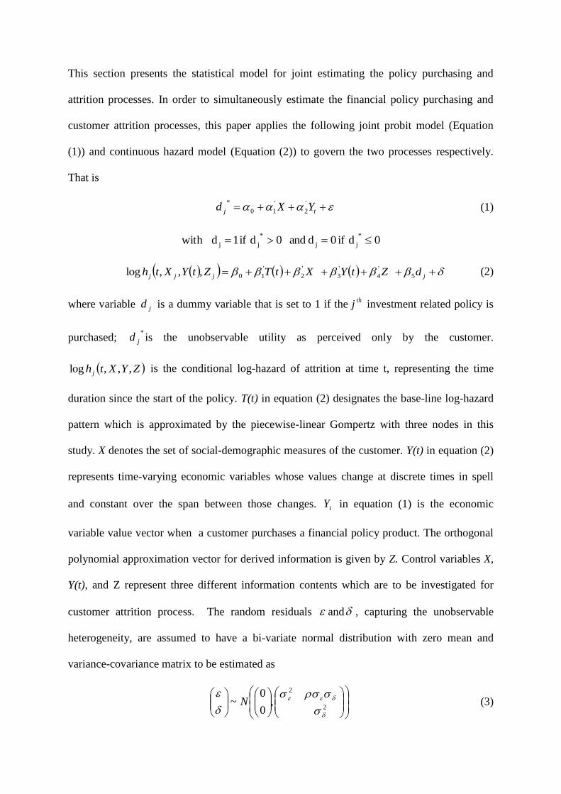
This section presents the statistical model for joint estimating the policy purchasing and
attrition processes. In order to simultaneously estimate the financial policy purchasing and
customer attrition processes, this paper applies the following joint probit model (Equation
(1)) and continuous hazard model (Equation (2)) to govern the two processes respectively.
That is
tj YXd '
2
'
10
* (1)
0d if 0d and 0d if 1dwith*
jj
*
jj
jjjj dZtYXtTZtYXth 5
'
4
'
3
'
2
'
10,,,log (2)
where variable jd is a dummy variable that is set to 1 if the jth
investment related policy is
purchased; *
jd is the unobservable utility as perceived only by the customer.
ZYXth j ,,,log is the conditional log-hazard of attrition at time t, representing the time
duration since the start of the policy. T(t) in equation (2) designates the base-line log-hazard
pattern which is approximated by the piecewise-linear Gompertz with three nodes in this
study. X denotes the set of social-demographic measures of the customer. Y(t) in equation (2)
represents time-varying economic variables whose values change at discrete times in spell
and constant over the span between those changes. tY in equation (1) is the economic
variable value vector when a customer purchases a financial policy product. The orthogonal
polynomial approximation vector for derived information is given by Z. Control variables X,
Y(t), and Z represent three different information contents which are to be investigated for
customer attrition process. The random residuals and , capturing the unobservable
heterogeneity, are assumed to have a bi-variate normal distribution with zero mean and
variance-covariance matrix to be estimated as
2
2
,0
0~
N (3)

where ρ is the correlation coefficient between the unobservable heterogeneity terms of the
two processes. The hazard rate of attrition, given by equation (2), is a function of social-
demographic variables X, time-varying macro-economic variables Y, and derived variables Z.
Thus, each group of variables provides insights about the directly observable ‘static’,
‘dynamic’ and unobservable derived information, respectively. In addition, including
component d in equation (2), allows us to analyze the impact of the kind of purchased policy
on the risk of attrition.
After estimating relevant parameters, we can calculate the predicted survival
probability for each customer in the holdout sample. The analysis applies the Nelson-Aalen
estimate of the baseline cumulative hazard function. Collett ((2003), p.257-258, eq.8.3 and
eq.8.5) provides details of the calculations. Considering there are n customers, among whom
there are r distinct attrition times and rn right-censored survival times. Then the base
cumulative hazard function for tH 0 is obtained as
J
j
tRl l
j
j
tx
etStH
1
00
exp
log
(4)
for 1 JJ ttt , 1,,2,1 rJ , where tS0 is the baseline survivor function, jtR is the
group of customers who are still with the company at a time just prior to jt , txl is the
vector of explanatory variables for the thl customer at time t, and je is the number of events at
the thj ordered event time, rj ,,2,1 . With this in hand, we obtain the approximate
conditional probability of surviving through the interval htt , for customer i in the sample
(Here we let 1h )
txtHhtHhttP ii exp}{exp, 00
~
(5)

5. Estimation results
Approximately 70 percent from the whole dataset, drawn randomly, forms the
training sample for model estimation. The remainder forms the holdout validation set used to
further refine and examine the accuracy of the model. The training dataset provides the data
for estimating the model while the holdout dataset provides the data for comparing the
predicting performance with and without the derived information. Table 3 presents the joint
maximum likelihood estimates for the joint probit- hazard multi-process models with and
without derived information using aML (Lillard and Panis, 2003). In Table 3, Panel I reports
the coefficient estimates for the policy purchasing and customer attrition processes. Panel II
presents the results for heterogeneity and correlation coefficient components.
Table 3 here
The coefficients for the baseline log-hazard are all statistically significant in
all periods. The attrition risk of the first 12 months rises (slope 1 = .08), it continues to rise
further and more sharply (slope 2 = .11) reaching a maximum at about 18th
month. Then the
attrition rate decreases until the 24th
month (slope 3 = -.13). However after two years, the
attrition rate again rises sharply (slope 4 = .23). The estimation results indicate that the
probability of purchasing investment policies and the risk of attrition are affected by social-
demographic variables. The dummy variable for gender, male, is significantly positive for
customer duration processes (.14). This suggests that male customers have a 15% (exp(.14)-
1) higher attrition rate than female customers. Not surprisingly, married customers seem more
risk averse than unmarried customers. Married customers are far less likely to invest in risky
investment policies, probably due to having children. They tend to keep a longer relation
with the financial insurance firm. The impacts of other social-demographic variables on each
process are slightly different. Dummy variables for age, financial status, and region

categories are used as indicators of customer social backgrounds. The customer’s age plays a
significant role in the rate of attrition. Those aged between 35 and 55 have the lowest attrition
rate compared with other age brackets. Customers in the highest financial bracket (financial
A) have an attrition risk that is 17% less than the reference, financial B customers. The
attrition hazard risk of customers with low financial status (financial C or beyond) rises to
19.2% above that of financial status B customers. Another interesting finding is that the rate
of attrition seems to be the same for all customers no matter which geographical area they
come from within the UK. The attrition rate for monthly payment customers rises by nearly
169% compared with other frequency payment customers when other things are equal. The
empirical results are consistent with previous literature, providing some support for the first
set of hypotheses in that customer demographics are related to attrition behaviour. The set of
coefficients that measure the effect of economic conditions are all significantly different from
zero except for the customer confidence index variable. This suggests that perceptions of the
national economy are related to the hazard rate of customer attrition. The coefficient that
captures the influence of the stock market is consistently negative with values around -2.32,
implying that, on average, customers’ attrition risk declines by 90 percent when the stock
market goes up. This is not a surprising result in that the value of financial policies tends to
increase with a rising stock market. The housing market does not have such a dramatic
impact as the stock market. However, the estimated coefficient (-.01 with a t-value of -3.34)
still implies the risk of attrition declines significantly with the rising of the housing market.
The interest rate has higher impact on attrition than house price. Overall, the results support
Hypothesis 2 that external macroeconomic environment influence financial customers’
attrition behaviour. When comparing the magnitudes and significance of relevant estimated
coefficients, there are almost no differences between the models with and without the derived

information except for the variable of “policy”. The effect of this variable becomes
insignificant when adding derived information. This might be due to the fact that ???
The estimated correlation coefficient
measures the association between the policy
purchase decision and the hazard rate of attrition. The result with respect to the significance
of
shows the presence of statistically significant systematic factors driving the two
processes (equal to .29 and .36 for without and with derived information, respectively). The
non-zero correlation between heterogeneity components of and indicates that customers
with a higher probability of purchasing investment policies also tend to have higher risks of
attrition. A key advantage, therefore, of the joint estimation approach is that it can control the
potential problem of endogeneity such as that noted by Boyes and Low (1989). Another
advantage is that it can easily accommodate the unobservable heterogeneity that affects both
policy purchase and attrition processes. The significance of heterogeneity component for the
hazard rate function 2
(equal to 1.65 and 1.63 for with and without derived information)
suggests that there is substantial unobservable heterogeneity in the risk of attrition after
allowing for both observable and derived covariates. Since the estimates are consistent both
with derived information and without derived information, the following discussion limits
itself to the effects of the variables in the model with derived information.
The main objective in deriving information from the value of financial policy
holdings is to evaluate customers’ attrition to the firm. Some customers re-invest the income
generated from the policies each month. The value of these policies will therefore change
month on month. This could be a reflection of customers slightly increasing their attrition
behaviour to the firm. On the other hand, if the value of policy holdings changes quite
considerably, this is likely to be as a result of customers increasing/decreasing their premiums
(when customers stop paying premiums, their policy holdings will drop to zero and the

relation with the firm is terminated). Studying the movement of policy holdings and
identifying what is income re-investment and what is increased/decreased premium provides
valuable insights for understanding and predicting customers’ attrition behavior.
Indicators of information derived from the value of policy holding values form the
parameters of the four main orthogonal components: absolute level, that is the latest financial
policy holding (there could be various ways of representing this component, such as the
average or weighted average of holdings over the time of duration); linear holding, that is
holding trend; quadratic holding, that is the holding curvature, and cubic holding, that is the
change of holding curvature. The significant impacts of some components of risk attrition
demonstrate that it is important to account for this derived information. The increasing order
of orthogonal components in terms of statistical significance appears to mitigate the effects of
derived information (this explains why an orthogonal polynomial approximation of order 3 is
applied).
The absolute level effect on the risk of attrition is significantly negative at any
reasonable level (-.65 with a t-value of being -3.5). This implies that the higher the
customer’s absolute value of policy holdings, the less likely he or she is to terminate the
relation with the firm. A higher value of policy holdings means that the customer puts more
money into the policy he or she purchased. This usually suggests that the customer expects
that the return for the customer will rise with the rise in value of the policy held. Thus the risk
of terminating the relation with the firm declines.
The linear effect of holdings is divided into two parts: linear trend up and linear trend
down (see definitions at the end of section 3). The coefficient for the increasing linear
component is significantly negative at 1% level (-1.87 with a t-value of -18.1). This indicates
an inverse relation exists between the risk of attrition and the increase in value of policy
holdings. The reason why policy holdings increase linearly is that the customer puts money

into the policy regularly and purchases a set amount of holdings, suggesting that the customer
commits more to the firm as the holdings increase. As a result, the customer’s holdings
increase irrespective of the movements in the market. It should be noted that the value here
refers to real holdings that exclude the market effects of fluctuating fund values.
Surprisingly, decreasing holdings also reduce the risk of attrition (-.43 with a t-value
of -5.20). The most likely reason for decreasing policy holdings is that the customer takes out
a regular fixed income from the policy. For example, a customer could take fixed funds out of
the investment each month (e.g. £500) to use as a regular income. As a result, although the
value of holdings declines at a constant rate, this is not an indication of decreasing customer
commitment to the firm.
Policy holders can decide the rate at which they increase or decrease the premiums of
their policy holdings. By calculating higher order orthogonal components, the analysis
captures dramatic increases and decreases in premiums. The nonlinear quadratic down
component is significantly positive at 5% level (12.95 with a t-value of 2.28) while the
quadratic up and cubic down components are statically insignificant but have expected signs.
This suggests that if a customer takes out income from the policy at a rate which exceeds the
rate at which the policy is growing or reduces premiums dramatically, the risk of attrition
increases significantly such that the customer will soon terminate the relation with the firm.
The cubic up component is also statistically significant (-4.64 with a t-value of -2.52),
suggesting the risk of attrition declines as the value of the holdings rises at a higher
accelerated rate. To what extent the additional derived information variables to reduce the
unexpected variation in the dependent variable can be measured by McFadden pseudo 2R .
Menard (2000) suggests that McFadden pseudo 2R satisfy all of Kvalseth (1985)’s eight
criteria for a good 2R . The McFadden pseudo 2R results show that the value of 2R with derived
information increases from 0.114 to 0.122 when derived information variables are included.

One reason for the relatively low 2R values is that we are dealing with individual customers
who reveal limited information. A significant improvement on 2R would require an
abundance of personal information. Nevertheless, these empirical results clearly show that
different orders of components derived from orthogonal polynomial approximation show
different customer attrition behavior patterns, therefore providing support the third
hypothesis.
Although research techniques in the behavioural finance literature are increasing in
efficiency and sophistication, there is still room for further improvement, not only in terms of
model fitting but also in terms of the efficient use of information. In particular, the
information conveyed by non-directly observable information can add explanatory power for
estimating risk attrition. The results of the explanatory variables highlight the potential
benefits of using derived information. The derived information would predict attrition several
months prior to a customer’s departure through identifying within the customer’s account if,
for example, deductions begin to fall off and assets begin to decrease dramatically. The
results can also have substantial practical value, as they change our views on how to obtain
relevant information signals in order to better understand customer attrition behavior. A
financial service firm can assess and monitor the behavior of its customers more accurately in
future through gathering such signals such as how customers change the value of their
policies. Financial service firms that invest in acquiring non-observable information can
apply and design more effective marketing strategies, such as cross-selling a particular
financial policy which satisfies customers’ special needs, in order to retain customers. Above
all, better screening and monitoring of customers can provide a firm with a competitive
financial advantage over its rivals.

6. Comparison of predictive performance
To assess the overall model fit, the analysis conducts in-sample tests comparing the
model with derived information to the nested model without derived information by applying
log-likelihood ratio test. A log-likelihood ratio test shows that the model incorporating
derived components outperforms the model with only demographic and economic covariates.
This suggests that the derived information plays an important role in explaining the
probability of customer attritions (LL = -36347.78 with derived information and LL = -
36687.00 without derived information, 6782 , degree of freedom = 7, p < .01).
Making predictions is one of the fundamental objectives for financial service industry
(Neslin et al. 2006). To further validate the results, this section assesses the importance of
incorporating this information by comparing the predictive power of the models with and
without the derived information. First, the analysis includes calculating predicted survival
probabilities for each customer in the holdout sample using the estimated coefficients for the
models with derived components and the model without derived information from Table 2.
In the analysis this study uses all but the last observation for each customer to calculate
predicted survival probabilities for next month.
Finally the analysis ranks customers in ascending predicted survival probabilities.
Customers with lower predicted survival probabilities are more likely to terminate the
relation with the firm for the specified time period. The model without derived information in
general correctly predicts 62.47% (2,206 out of 3,531) terminating customers. The model
with derived information correctly predicts 64.37% (2,273 out of 3,531) terminating
customers, suggesting it has a 1.90% better prediction rate than the model without derived
information. This difference is economically significant for financial institutions considering
the potential number of customers, which not only lead to a substantial increase in profits but
also provide competition advantage for those institutions that retain customers better. The

cut-off for classifying terminating and continuing customers is the ex-post proportion of
attrition in the holdout sample (3,531/7,498 = .47 the hazard rate). The hazard rate model
with derived information predicts only marginally better than the one without derived
information. However, an accurate assessment of the probability of attrition in retail sale can
give a financial firm a considerable competitive advantage over other firms. Even a small
improvement of predicting the probability of attrition could bring financial service firms
substantial increases in profits (Blochlinger and Leippold, 2006).
The forecasting power of derived information in distinguishing between low and high
attrition risk customers can also be estimated by using the Receiver-Operator Characteristic
(ROC) analysis. The ROC curve is a plot of true positive rate, tp, (i.e., the number of known
survivors classified as survivors over total number of known true survivors) on the x-axis
versus false positive rate, fp, (i.e., the number of known attritions classified as survivors over
total number of true attritions) on the y-axis for all possible values of decision thresholds. We
first sort the predicted survival probability for each customer in the holdout sample in
ascending order. The actual dummy attrition indicator (i.e., )0;1 attritionsurvivor is then
sorted accordingly for each customer. The ROC curve is independent from the decision
thresholds and the further the curve away from the 45-degree diagonal, the higher the
predictive power.
In order to examine the consistency of the model’s performance, we further conduct non-
parametric bootstrap simulation to explore whether the higher predictive power using derived
information arises by fortunate selection of the training and validation data sets. Efron (1981)
introduces an algorithm in which the non-parametric bootstrap analysis is used for censored
data. The non-parametric bootstrap is a simulation where we resample with replacement from
the original sample. Specifically, the bootstrap simulation procedure is conducted as follows:

i. Based on the original data provided by the insurance company, we sample with
replacement form the original data to get a new bootstrap sample. Thus, some
customers will be selected more than once in this new sample or perhaps not at all.
ii. We then randomly split of the new bootstrap sample into new training and new
validation data.
iii. The new training sample is then used to estimate the hazard model for both models
with derived components and the model without derived information. With the
relevant estimated coefficients we calculate bootstrap predicted survival probabilities
for each customer in the new validation data. Using the bootstrap replicates of
predictive survival probabilities, we then calculate the area under the ROC curves
(AUC), which is a commonly used summary measure of predicting effectiveness.
The value for the area under the ROC curve closing to 1 indicating perfect predicting
effectiveness and 0.5 indicating the same accuracy as random guess.
iv. Replicating steps i through iv 1000 times.
Figure 2 here
Figure 2 presents the ROC curves for models with and without adding derived
information in the holdout sample. In general, the model with the seven derived variables
performs marginally better than the model without the derived information. However, it
should be noted that there are three crosses for the ROC curves at three different decision
thresholds especially for the second crossing point. This indicates that the model with the
derived information is not uniformly better than the model without the derived information.
Both the overall model fit test and the forecasting analysis reliably show the marginal
improvement of the use of derived information in predicting customer attrition probabilities.
We obtain that the average AUC value for hazard model with derived information is 0.6919
and without derived information is 0.6671. This supports the analysis above that the better

prediction of using derived information does not arise by ‘fortunate’ selection of the training
and validation sets. Our results confirm Johnson et al. (2006) that derived variables through
orthogonal polynomial approximations can produce better predicting probabilities. Though in
a different setting, both this study and Johnson et al. (2006)’s study confirm that people are
more effectively in discounting directly observable information than less directly observable
information. Overall, the results of the bootstrap simulation analysis provide further evidence
that the additional derived information can be exploited for financial service industry to better
understand customer attrition behavior.
It has been proposed that simpler logistic or probit model can achieve similar
predictive performance to complex models such as hazard model (Lee and Urrutia 1996).
This leads us to a further demonstrate the added value of derived information on simple
logistic model (Occam’s razor). We conduct the bootstrap simulation from step i to iv except
that the third step is for logistic model rather than for hazard model. However, it should be
noted that time-dependent macro-economic variables cannot be estimated for logistic model
while hazard model can handle time-dependent variables easily which is an advantage of over
logistic model. Another advantage of hazard model is that it can take into account of
censoring variables. The ROC curve for logistic model with and without derived information
is presented in Figure 3.
Figure 3 here
The average SUC value for logistic model with derived information is 0.6920 and that of
without derived information is 0.6456, suggesting better predictive performance of derived
information.
7. Conclusion

The value of customer has been widely recognised in terms of financial planning and
efficient resource allocation. Customers are increasingly mobile and ever-more demanding.
Understanding customer attrition behaviour has been the subject of considerable prior
research; most research focus on using directly observable and commonly used information
such as geographic, demographic and macroeconomic variables. This paper has demonstrated
the value of derived information. The results of the study have implications for researchers in
two broad areas. First, they provide evidence of the need to take customers’ financial
behaviour into account when attempting to investigate and predict customer attrition. While
demographic and external economic environment can certainly affect customer attrition
behaviour, it seems that in mature markets such as the one we examined, customer attrition
behaviour is also driven by the customer’s own experiences of the value of financial
products.
The second area of implication for researchers relates to the study’s contribution to
the introduction of a statistical approach for deriving certain behavioral factors which
measure customers’ attrition behaviour to financial firms. This approach expands traditional
views on the use of information in customer attrition and could be applied to areas of finance
in which efficient use of information is involved, such as the subject of behavioral finance. In
that context, the statistical techniques applied in this paper have been seen to be useful, and
their application to the study of the behavior of financial customers and the subsequent effect
on financial markets will be rewarding.
The findings of the study also have implications for financial services industry which
is competing intensely for opportunities for financial product sales and customer loyalty. In
addition to capturing customers’ financial behavior changes, our findings clearly show that
derived information can achieve nominally small but managerially meaningful increases in
predictive accuracy. This suggests that customer behavior is a good source of information

about their priorities, needs, and experiences. Therefore, financial firms should manage
customer experience and collect more relevant information on the financial behaviour of
customers for analysis if they desire to have a competitive advantage over other financial
firms and increase the value of customers. Customer attrition can have a significant impact on
profitability for financial firms. If derived information indicates that a customer might leave,
financial firms are able to implement meaningful retention strategies and extend customers’
lifespan by creating or offering new financial products with a focus on customer experience,
flexibility, and appropriate pricing.
The limitations of the study in respect of the relatively small sample and the focus on
only one financial firm suggest that the findings here needed to be primarily seen as
exploratory. Further research is suggested that using data from other financial firms can
generalize and strengthen our knowledge of derived information on customer attrition.
Another area of interest concerns the contagion of customers’ attrition decision. Analysis of
this issue is beyond the scope of this paper, but this is an area for further research that would
have clear managerial implications. The financial policy product market examined in this
study is a mature market. Customers do not leave the market altogether but simply follow
others to switch to competitors. Therefore, it might be worthwhile to collect this type of
behaviour information.

Appendix
Based on the observed monthly financial policy holding values
))}1(),1((;));1(),1({( kk nuntut for customer k, a sequence of orthogonal polynomials f0, f1, f2,
. . . exists and satisfies
0))(())((1
1
kn
l
ji ltfltf for all ji . (A1)
There is a unique set of coefficients a0, a1, a2, and 3a following
3
0
))(()(i
ii ltfalu for all 1,,1 knl . (A2)
ai can be found by least squares. As the fi are orthogonal, ai signifies the size of the order i
component in the holding value. Because of the importance of the final holding value
,1knu let f0(t(n)) = f0(1) = 1 and fi(1) = 0 for all i ≥ 1, we make the level component a0
equal to u(( 1kn )). This study also normalizes each fi so that its leading term is simply ti. a1
is the slope of the least squares regression line constrained to pass through )1(),1( kk nunt .
a2 measures the holding curve curvature and a3 measures the change in curvature. Thus, the
values of a1, a2, and a3 can be used to gauge customers’ attrition to the financial firm. We
illustrate the unit holding values, linear trend, quadratic and cubic approximations for a
randomly chosen customer in Figure 4. Note we scale the times so that 0)1( t and 1)1( knt
Figure 4 here
When the number of monthly holding values, n, is small for customer k, a2 and a3 will
change dramatically if a small change in one of the holding values. A roughness penalty can
mitigate this. Let
3
0)()(
i ii tfatF , then choose the ai to minimize
)()))(()((1
1
2 FGltFlukn
l
(A3)

where G(F) is the roughness penalty and λ is some constant of proportionality. Here let G(F)
equal to the area of F above umax = max u(i) and below umin = min u(i). That is,
1
0
min
1
0
max )0),(max()0,)(max()( dttFudtutFFG . (A4)
In addition, the approximation incorporates two refinements of the parameter set based on our
understanding of how holdings behave in practice. Since high value holdings change by
larger amounts than low values, the relative size is thus more important than the absolute size
of any change. Consequently, before calculating parameters a1, a2, a3, the holding curve
{(t(1),u(1)); . . .; t( 1kn ),u( 1kn ))} is rescaled by dividing u(i) by u(n k -1) for kni ,,1 .

References
Athanassopoulos, A. (2000). Customer satisfaction cues to support market segmentation and
explain switching behaviour. Journal of Business Research 47, 191-207.
Blochlinger, A. Leippold, M. (2006). Economic benefit of powerful credit scoring. Journal
of Banking and Finance 30, 851-873.
Bolton, R. Kannan, P. Bramlett, M. (2000). Implications of loyalty program membership and
service experiences for customer retention and value. Journal of the Academy of Marketing
Science 28, 95-108.
Bose, I. Chen, X. (2009). Quantitative models for direct marketing: A review from systems
perspective. European Journal of Operational Research 195, 1-16.
Boyes, W. Low, H. (1989). An Econometric analysis of the bank credit scoring problem.
Journal of Econometrics 40, 3-14.
Buckinx, W. Van den Poel, D. (2005). Customer base analysis: partial defection of
behaviourally loyal clients in a non-contacted FMCG retail setting. European Journal of
Operational Research 164,252-268.
Chen, Z. Fan, Z. Sun, M. (2012) A hierarchical multiple kernel support vector machine for
customer churn prediction using longitudinal behavioural data. European Journal of
Operational Research 223, 461-472.
Collett, D. (2003). Modelling survival data in medical research. Chapman & Hall.
Dekimpe, M. Degraeve, Z. (1997). The attrition of volunteers. European Journal of
Operational Research 98, 37-51.
Efron, B. (1981). Censored data and the bootstrap. Journal of the American Statistical
Association 76, 312-319.
Ganesh, J. Arnold, M. Reynolds, K. (2000). Understanding the customer base of service
providers: An examination of the differences between switchers and stayers. Journal of
Marketing 64, 65-87.
Glady, N. Baessens, B. Croux, C. (2009). Modelling churn using customer life time value.
European Journal of Operational Research 197, 402-411.
Johnson, J. Jones, O. Tang, L. (2006). Exploring decision makers’ use of price information
in a speculative market. Management Science 52, 897-908.
Keaveney, S. (1995). Customer switching behavior in service industries: An exploratory
study. Journal of Marketing 59,71.82.
Kvalseth, T. (1985). Cautionary note about 2R . The American Statistician 34, 274-285.

Lee, S. Urrutia, J. (1996) Analysis and prediction of insolvency in the property liability
insurance industry: A comparison of logit and hazard models, Journal of Risk and Insurance
63, 121-130.
Lessmann, S. Vob, S. (2009). A reference model for customer-centric data mining with
support vector machines. European Journal of Operational Research 199, 520-530.
Lillard, L. Panis, C. (2003). aML multilevel multiprocess statistical software, Version 2.0,
EconWare, Los Angeles, California.
Menard, S. (2000). Coefficients of determination for multiple logistic regression analysis.
The American Statistician 54, 17-24.
Mittal. V. Kamakura, W. (2001). Satisfaction, repurchase intent, and repurchase behaviour:
Investigating the moderating effect of customer characteristics. Journal of Marketing
Research 38, 131-142.
Neslin, S. Gupta, S. Kamakura, W. Lu, J. Mason, C. (2006). Defection detection: Measuring
and understanding the predictive accuracy of customer churn models. Journal of Marketing
Research 43, 204-211.
Tang, L. Thomas, S., Thomas, L, Bozzetto, J. (2007). It’s the economy stupid: Modelling
financial product purchases. International Journal of Bank Marketing 25, 6-22.
Thomas, L. Thomas, S. Tang L. Gwilym, O. (2005). The impact of demographic and
economic variables on financial policy purchasing timing decisions. Journal of Operation
Research Society 56, 1051-1062
Thomas, L. (2010). Consumer finance: challenges for operational research. Journal of the
Operational Research Society 61, 41-52.
Van den Poel, D. Lariviere, B. (2004). Customer attrition analysis for financial services
using proportional hazard models. European Journal of Operational Research 157, 196-217.
Wetherill, B. (1981). Intermediate Statistical Methods, Chapman and Hall, London.
Verbeke, W., Dejaeger, K. Martens, D. Hur, J. Baesens, B. (2012). New insights into churn
prediction in the telecommunication sector: A profit driven data mining approach. European
Journal of Operational Research 218, 211-219.

Table 1: Number of policy changes from April 2001 to March 2004
Apr01-Mar 02 Apr 01-Mar 03 Apr01-Mar 04
Total number of policies purchased
purpurchased purpurchasedpolicy
ppurchased
18,270 20,224 20,257
Of which: Investment 15,255 16,560 16,578
Non-investment 3,015 3,664 3,679
Total number of policies terminated 2,588 6,171 10,050
Of which: Investment 2,412 5,603 9,180
Non-investment 176 568 870
Total number of policies continued 15,682 14,053 10,207
Of which: Investment 12,843 10,957 7,395
Non-investment 2,839 3,096 2,812

Table 2: Definitions of the three sources of explanatory variables.
This table lists three sources of explanatory variables. The first source is social
demographic variables provided by the UK financial insurance company. The second
source is external economic variables. The economic variables are obtained from
Datastream. The third source of explanatory variables is derived variables through
orthogonal polynomial approximations. There are 22 explanatory variables including
15 directly observed and 7 derived variables. Variables Definitions
(1). Social demographic
Male A dummy variable of customer’s gender. 1 if the customer is male,
otherwise 0.
Mariage A dummy variable of customer’s marriage. 1 if the customer is married,
otherwise 0.
Age between 20 and 35 A dummy variable of customer’s age. 1 if age is between 20 and 35,
otherwise 0.
Age between 35 and 55 A dummy variable of customer’s age. 1 if age is between 35 and 55,
otherwise 0.
Age above 55 A dummy variable of customer’s age. 1 if age is above 55, otherwise 0.
Financial status A A dummy variable of customer’s financial status. 1 customer’s financial
status is classified A , otherwise 0.
Financial status CD A dummy variable of customer’s financial status. 1 customer’s financial
status is classified CD , otherwise 0.
Scotland A dummy variable of customer’s region. 1 if customer is from Scotland,
otherwise 0.
England A dummy variable of customer’s region. 1 if customer is from England,
otherwise 0.
Monthly Payment A dummy variable of financial payment frequency. 1 if payment is monthly
and 0 if yearly.
Policy A dummy variable of financial policy being purchased. 1 if investment
policy is purchased, otherwise 0.
(2). Economy
Stock Return Logarithm of first difference of monthly FTSE All Shares index.
House Price First difference of monthly UK house price index.
Interest Rate Monthly Bank of England base interest rate.
Confidence Index Monthly of UK customer confidence index.
(3). Parameterized
Absolute Level The height of the holding values, i.e. the latest holding s.
Linear UP The linear orthogonal component with the value of holdings increasing.
Linear DW The linear orthogonal component with the value of holdings decreasing.
Quad UP The curvature (quadratic component) with the value of holdings increasing.
Quad DW The curvature (quadratic component) with the value of holdings
decreasing.
Cubic UP The change of curvature (cubic component) with the value of holdings
increasing.
Cubic DW The change of curvature (cubic component) with the value of holdings
decreasing.

Table 3: Estimation of the joint Probit-hazard model.
This table examines the effect of directly observable information on the choice of policy
purchasing applying Probit model and derived information on the probability of attrition
applying hazard rate regression. The coefficients are the joint maximum log-likelihood
estimates for the joint probit-hazard models in order to simultaneously estimate the
customer attrition process and the customer relations established during the initial process
of setting up the financial policy. Panel I reports the coefficient estimates for the policy
purchasing and customer attrition processes. Panel II reports the estimate results for
heterogeneity and correlation coefficient components. The sample period is April 2001 to
March 2004.
Variables Without derived information With derived information
Variable t-value Variable t-value Hazard ratio
Panel I: Financial policy purchase process (Probit)
Constant -4.95** -7.34 -5.12** -7.41 ---
Male 0.10 1.26 .09 1.19 ---
Mariage -3.01** -9.99 -3.03** -10.1 ---
Age between 20 and 35 -1.04** -4.14 -1.07** -4.02 ---
Age between 35 and 55 -1.30** -5.02 -1.33** -5.07 ---
Age above 55 -1.03** -4.08 -1.05** -4.14 ---
Financial Status A -.03 -.35 -.03 -.35 ---
Financial Status CD .12 1.21 .116 1.21 ---
Scotland .008 .05 .03 .09 ---
England .11 1.06 .1089 1.03 ---
Stock Return -11.98** -8.69 -12.10** -8.71 ---
House Price .156** 8.39 .159** 8.41 ---
Interest Rate 1.47** 8.83 1.51** 8.86 ---
Confidence Index -.32** -9.54 -.33** -9.56 ---
Attrition process (Hazard)
Constant -4.83** -14.8 -3.84** -11.6 .021
Male .11* 2.57 .14** 3.19 1.15
Marriage -.32** -4.18 -.34** -4.56 .712
Age between 20 and 35 -.45** -4.58 -.45** 4.61 .637
Age between 35 and 55 -.50** -5.59 -.51** -5.63 .601
Age above 55 -.29** -3.26 -.24* 2.68 .788
Financial status A -.19** 3.78 -.19** -3.65 .830
Financial status CD .19** 3.44 .18** 3.16 1.19
Scotland .01 .14 -.00 -0.04 .99
England -.09 -1.48 -.10 -1.53 .907
Monthly Payment .43** 7.11 .99** 13.9 2.69
Policy .52** 3.35 -.05 -0.32 .953
Slope1 .07** 6.88 .08** 7.78 1.08

Slope2 .11** 9.21 .11** 9.63 1.12
Slope3 -.12** -9.35 -.13** -9.82 .88
Slope4 .23** 30.4 .23** 31.2 1.26
Stock Return -2.42** -8.87 -2.32** -8.44 .10
House Price -.01** -3.24 -.01** -3.34 .99
Interest Rate -.15* -2.63 -.19** -3.31 .83
Confidence Index .00 .14 -.00 -0.35 1.00
Absolute Level --- --- -.65** -23.5 .52
LinearUP --- --- -1.88** -18.1 .15
LinearDW --- --- -.43** -5.20 .65
QuadUP --- --- -10.53 -1.29 .00
QuadDW --- --- 12.95* 2.28
CubicUP --- --- -4.6* -2.52 .01
CubicDW --- --- .11 .43 1.12
Panel II: Heterogeneity & correlation estimates
2
1.69** 20.3 1.70** 21.8 ---
2
1.63** 7.33 1.65** 7.41 ---
, .29** 4.51 0.36** 6.04
Log Likelihood with
covariates )( mL -36687.00 -36347.78
Log Likelihood with no
covariates )( 0L -41410.01 -41410.01
McFadden pseudo 2R 0.114 0.122
Notes: Asterisks * and ** indicate significance at the 5% and 1% levels; McFadden pseudo2R is defined
as 0lnln1 LLm

Figure 1: Survival distribution curve function for customer attrition
0 . 0 0
0 . 2 5
0 . 5 0
0 . 7 5
1 . 0 0
Du r a t i o n
0 5 1 0 1 5 2 0 2 5 3 0 3 5 4 0
L e g e n d : Pr o d u c t - L i mi t Es t i ma t e Cu r v e
Ce n s o r e d Ob s e r v a t i o n s
0 0.1 0.2 0.3 0.4 0.5 0.6 0.7 0.8 0.9 10
0.1
0.2
0.3
0.4
0.5
0.6
0.7
0.8
0.9
1
False Postive Rate
Tru
e P
ositiv
e R
ate
Figure 2: Predictive comparison of ROC using bootstrap
without derived information, AUC=0.6671
with derived information, AUC=0.6919

0 0.1 0.2 0.3 0.4 0.5 0.6 0.7 0.8 0.9 10
0.1
0.2
0.3
0.4
0.5
0.6
0.7
0.8
0.9
1
False Postive Rate
Tru
e P
ositiv
e R
ate
Figure 3: Predictive comparison of ROC using Logistic regression
without derived information. AUC=0.6456
with derived information. AUC=0.6920
0 0.1 0.2 0.3 0.4 0.5 0.6 0.7 0.8 0.9 16.4
6.6
6.8
7
7.2
7.4
7.6
7.8
8
8.2
8.4
Time
Log P
olic
y U
nit H
old
ings
Figure 4: Orthogonal polynomial approximations
Unit holdings
Linear trend
Quadratic
Cubic