Assessing the Health Effects of Air Pollution; Statistical and Computational Challenges

Scott L. Zeger on behalf of

The Environmental Biostatistics and Epidemiology Group (EBEG)The Johns Hopkins University

Bloomberg School of Public Health

CISES Meeting – Chicago

October, 2004

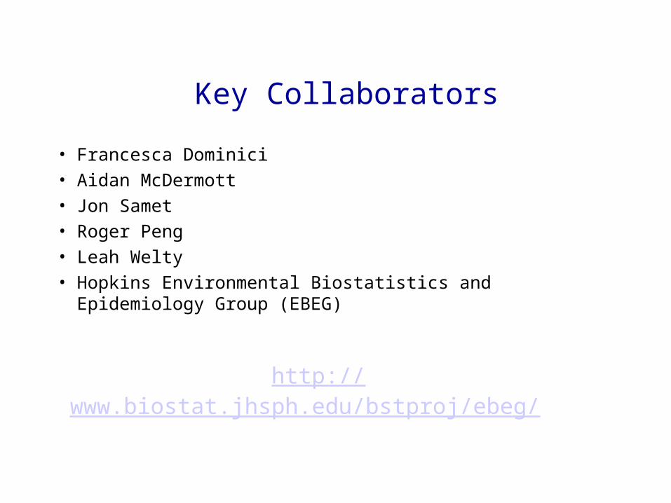
Key Collaborators

• Francesca Dominici

• Aidan McDermott

• Jon Samet

• Roger Peng

• Leah Welty

• Hopkins Environmental Biostatistics and Epidemiology Group (EBEG)

http://www.biostat.jhsph.edu/bstproj/ebeg/

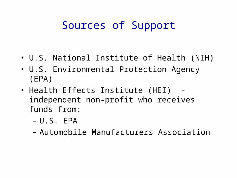
Sources of Support

• U.S. National Institute of Health (NIH)

• U.S. Environmental Protection Agency (EPA)

• Health Effects Institute (HEI) - independent non-profit who receives funds from:

– U.S. EPA

– Automobile Manufacturers Association

Outline

• Air pollution and mortality: a brief overview of the epidemiologic evidence– Cohort studies– Time series studies - NMMAPS

• Spatial-time series models– Temporal then spatial models

• Key statistical issues

• Toward reproducible research

Daytime in London, 1952

Source: National Archives

Particulate levels – 3,000 g/m^3

Designer Smog Masks - London 1950’s

Source: DL Davis. When Smoke Ran Like Water (2002)

~10,000 excess deaths

•4,000 first week

•8,000 over next 2 months

•Pollution or flu or both?

50th Anniversary Meeting

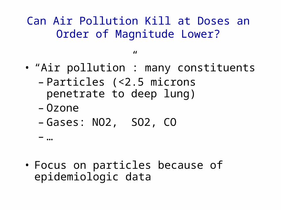
Can Air Pollution Kill at Doses an Order of Magnitude Lower?

• “Air pollution”: many constituents– Particles (<2.5 microns penetrate to deep lung)– Ozone– Gases: NO2, SO2, CO– …

• Focus on particles because of epidemiologic data

Key Epidemiologic Evidence

• Chronic exposures: cohort studies

– Six Cities Study (e.g. Dockery, et al , 1993)

– American Cancer Study (e.g. Pope, et al, 2002)

• Acute exposures: multi-city time series studies

– NMMAPS (90 U.S.cities; e.g. Samet, et al, 2000)

– APHEA (29 Eur cities; e.g.Katsouyanni, et al, 2003)

– CANADIAN (8 Cities; e.g. Burnett, Goldberg, 2003)

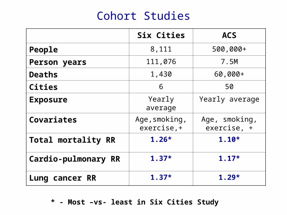
Six Cities ACS

People 8,111 500,000+

Person years 111,076 7.5M

Deaths 1,430 60,000+

Cities 6 50

Exposure Yearly average Yearly average

Covariates Age,smoking, exercise,+

Age, smoking, exercise, +

Total mortality RR 1.26* 1.10*

Cardio-pulmonary RR 1.37* 1.17*

Lung cancer RR 1.37* 1.29*

* - Most –vs- least in Six Cities Study

Cohort Studies

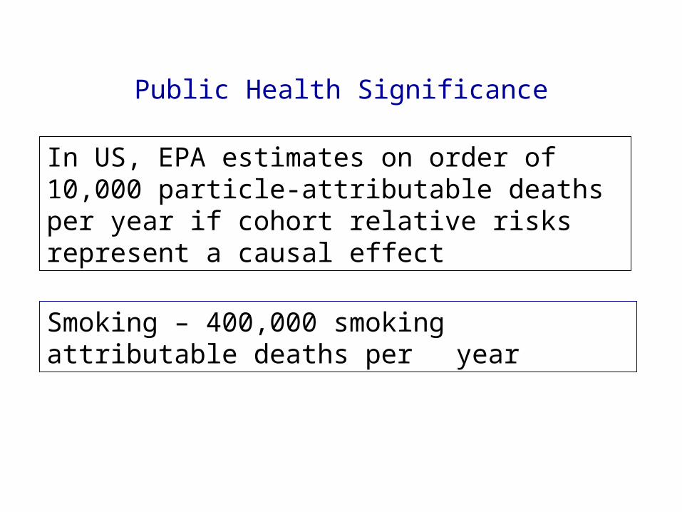
Public Health Significance

In US, EPA estimates on order of 10,000 particle-attributable deaths per year if cohort relative risks represent a causal effect

Smoking – 400,000 smoking attributable deaths per year

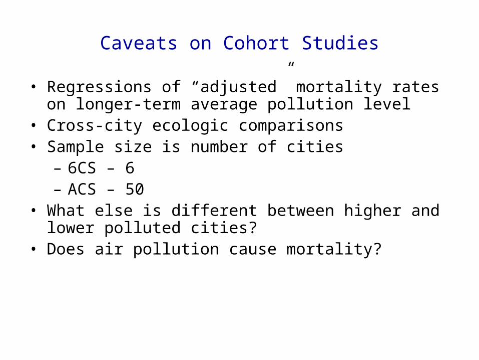
Caveats on Cohort Studies

• Regressions of “adjusted” mortality rates on longer-term average pollution level

• Cross-city ecologic comparisons• Sample size is number of cities

– 6CS – 6– ACS – 50

• What else is different between higher and lower polluted cities?

• Does air pollution cause mortality?

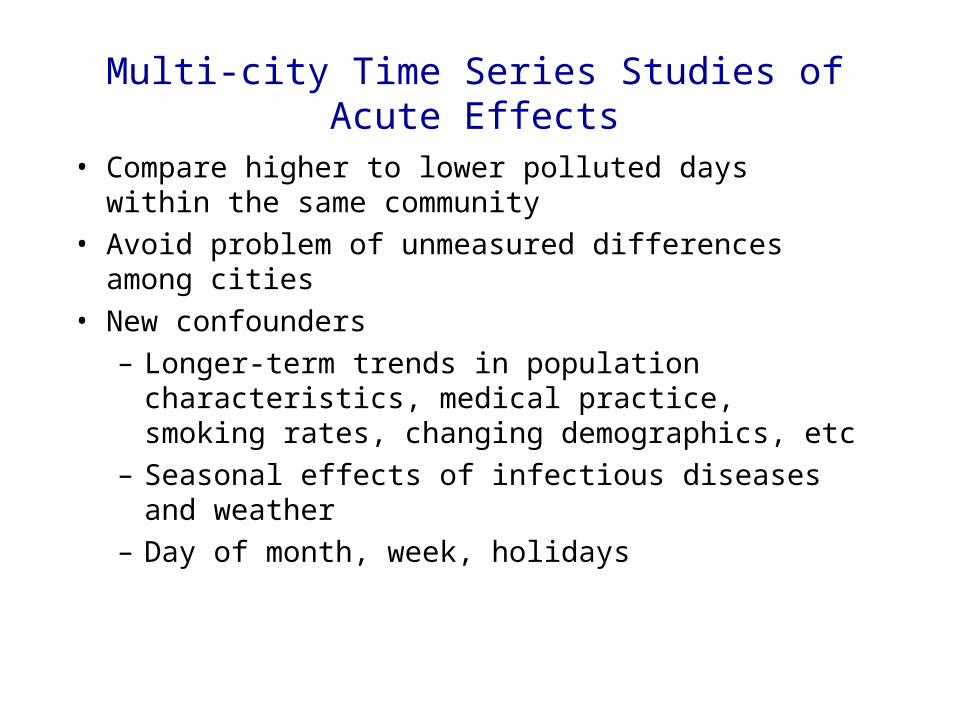
Multi-city Time Series Studies of Acute Effects

• Compare higher to lower polluted days within the same community

• Avoid problem of unmeasured differences among cities

• New confounders

– Longer-term trends in population characteristics, medical practice, smoking rates, changing demographics, etc

– Seasonal effects of infectious diseases and weather

– Day of month, week, holidays

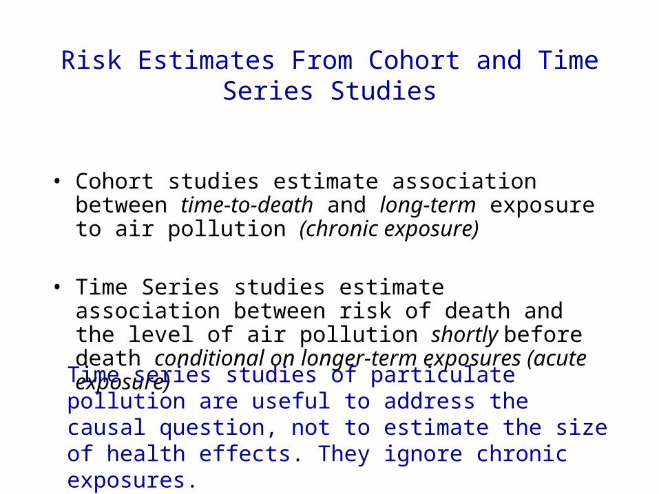
Risk Estimates From Cohort and Time Series Studies

• risks • Cohort studies estimate association between time-to-death

and long-term exposure to air pollution (chronic exposure)

• Time Series studies estimate association between risk of death and the level of air pollution shortly before death conditional on longer-term exposures (acute exposure)

Time series studies of particulate pollution are useful to address the causal question, not to estimate the size of health effects. They ignore chronic exposures.

National Morbidity and Mortality Air Pollution Study (NMMAPS)

• HEI funded collaboration of Johns Hopkins and Harvard Universities; Jon Samet, PI

• 90 largest U.S cities covering roughly 40% of annual deaths (now 105)

• 1987- 1994; now updated through 2001

• Mortality and hospitalizations (14 cities)

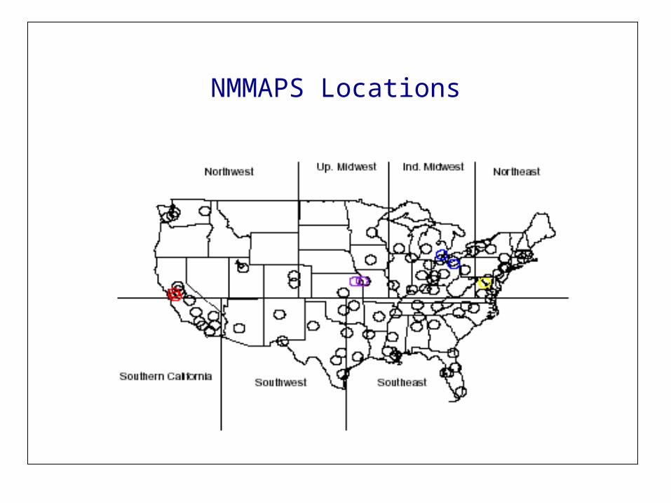
NMMAPS Locations

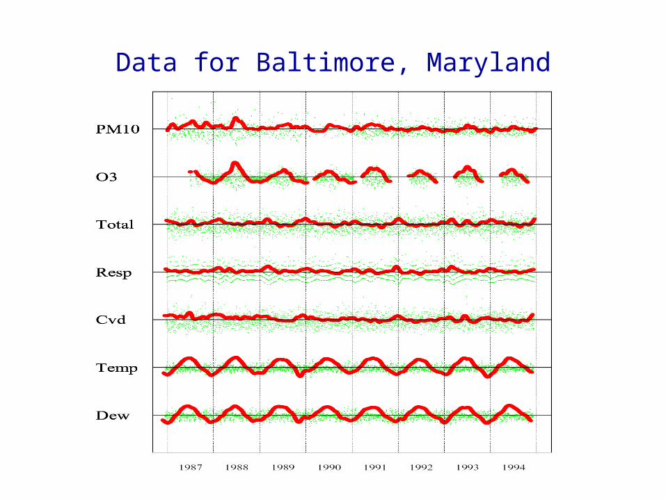
Data for Baltimore, Maryland

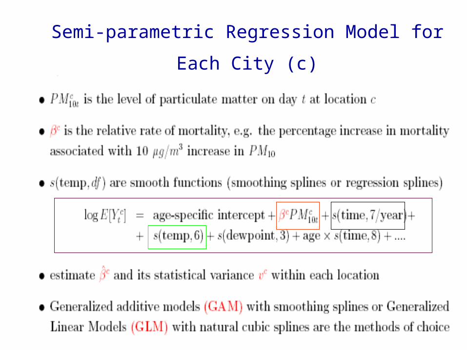
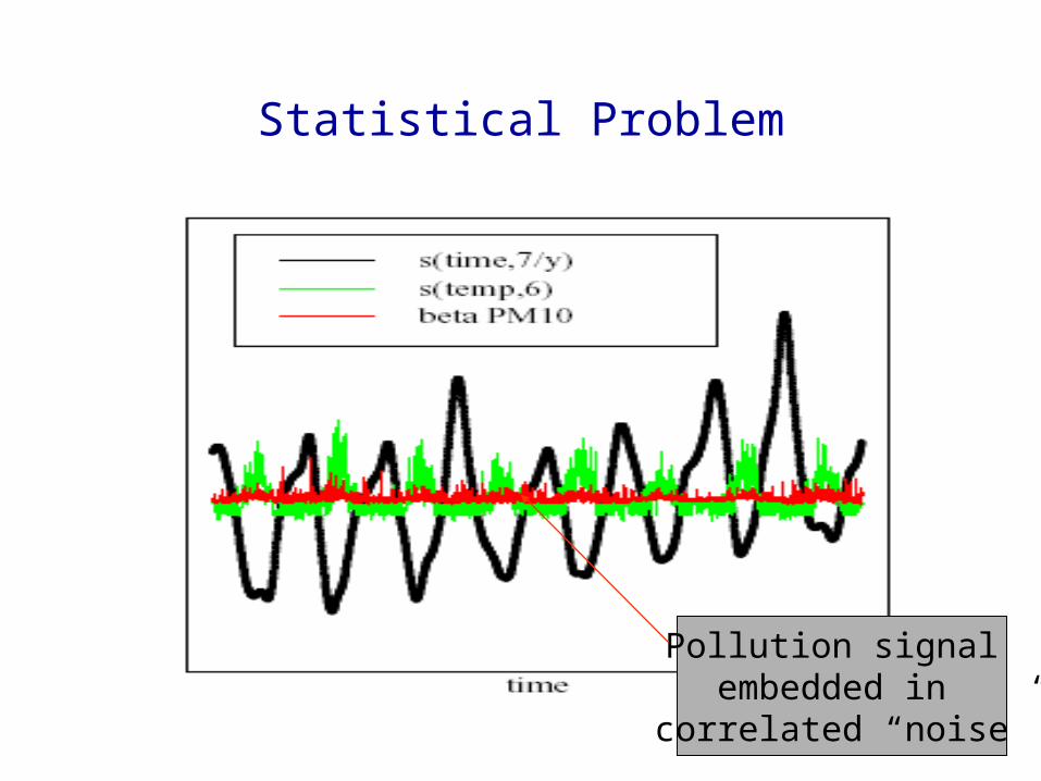
Semi-parametric Regression Model for Each City (c)

Statistical Problem

Pollution signal embedded in

correlated “noise”

City-specific Estimates

Map of City Specific Estimates

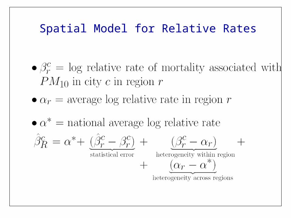
Spatial Model for Relative Rates

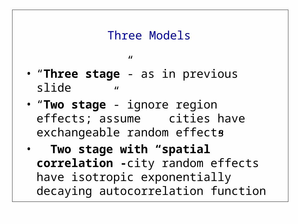
Three Models

• “Three stage”- as in previous slide• “Two stage”- ignore region effects; assume

cities have exchangeable random effects• Two stage with “spatial” correlation -city

random effects have isotropic exponentially decaying autocorrelation function

Joint Estimation of 90 City Slopes With Spatial Model

• Approximate the conditional distribution of each city estimate given its true value by a Gaussian model with mean and variance equal to the mle and inverse of Fisher information under an over-dispersed Poisson model

• No borrowing strength across cities for estimation of smooth functions of time and temperature (a full Bayesian analysis with “infinite prior variances for these terms)

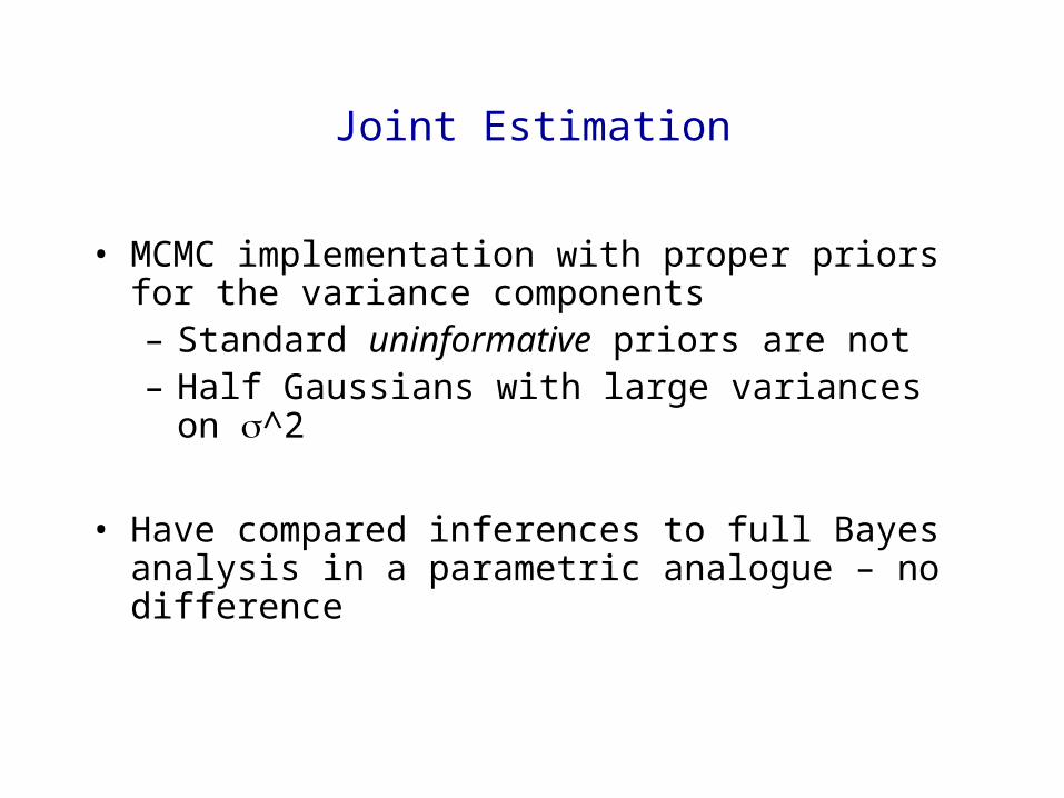
Joint Estimation

• MCMC implementation with proper priors for the variance components– Standard uninformative priors are not– Half Gaussians with large variances on ^2

• Have compared inferences to full Bayes analysis in a parametric analogue – no difference

Posterior Distribution of National Average

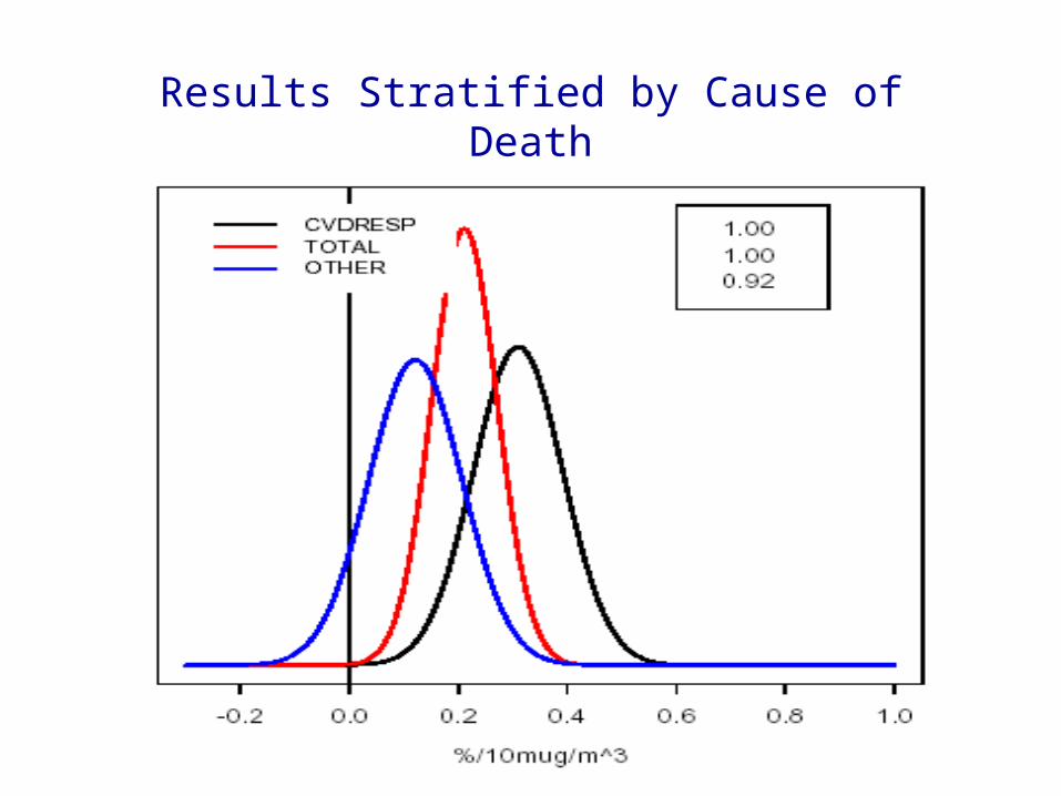
Results Stratified by Cause of Death

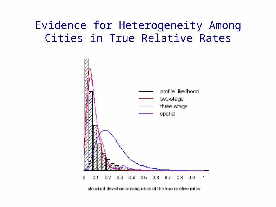
Evidence for Heterogeneity Among Cities in True Relative Rates

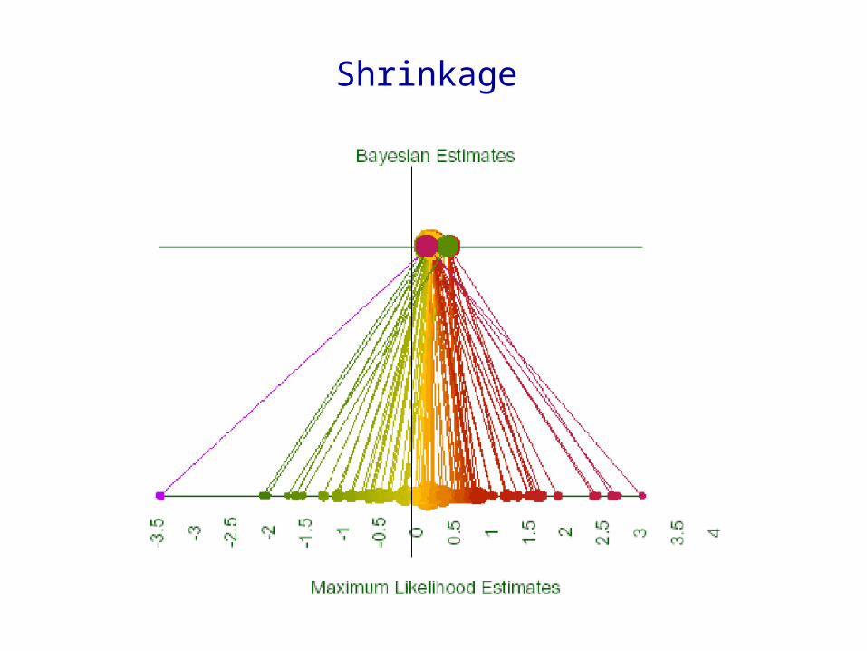
Shrinkage

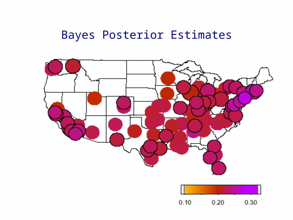
Bayes Posterior Estimates

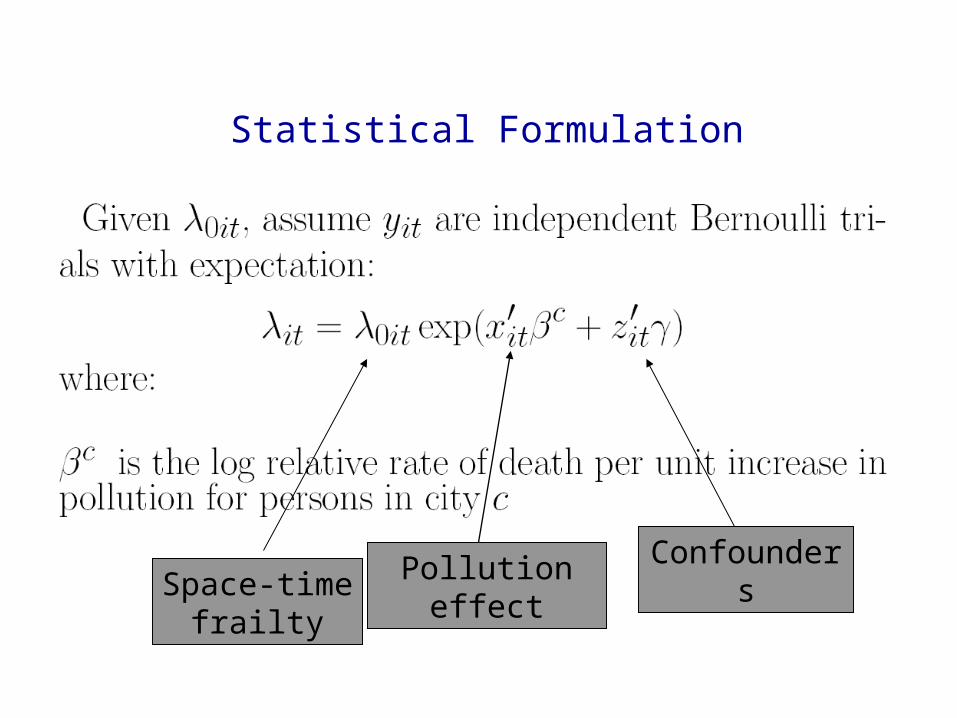
Statistical Formulation

Pollution effect ConfoundersSpace-time

frailty

Scientific and Statistical Issues

1. Model for the baseline frailty process and other unmeasured confounders process in space and time

– personal variables (smoking, exercise) – city-specific variables (demographics, medical services) – influenza epidemics

2. Co-pollutants 3. Public health significance: “harvesting?”4. Distributed lags5. Reproducible research

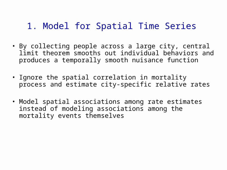
1. Model for Spatial Time Series

• By collecting people across a large city, central limit theorem smooths out individual behaviors and produces a temporally smooth nuisance function

• Ignore the spatial correlation in mortality process and estimate city-specific relative rates

• Model spatial associations among rate estimates instead of modeling associations among the mortality events themselves

Formulation of Time Series Model“Collect and Conquer”

Degree of Adjustment

Degree of Adjustment

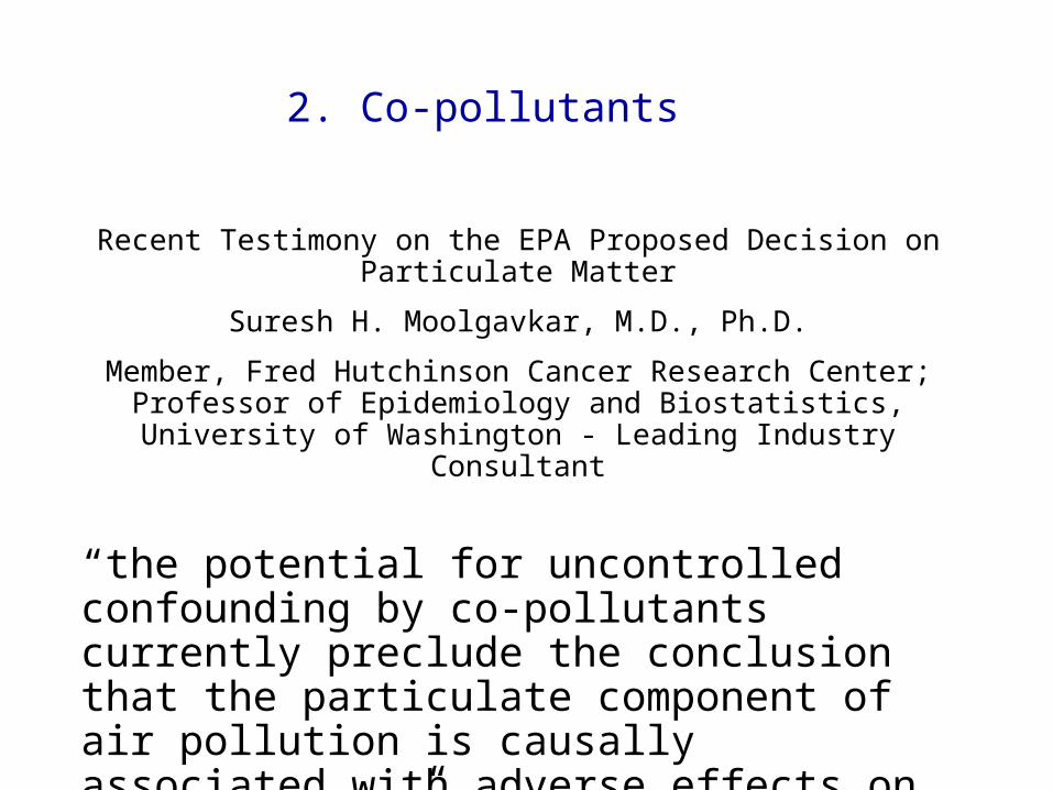
2. Co-pollutants

Recent Testimony on the EPA Proposed Decision on Particulate Matter

Suresh H. Moolgavkar, M.D., Ph.D.

Member, Fred Hutchinson Cancer Research Center; Professor of Epidemiology and Biostatistics, University of Washington - Leading

Industry Consultant

“the potential for uncontrolled confounding by co-pollutants currently preclude the conclusion that the particulate component of air pollution is causally associated with adverse effects on human health.”

Co-pollutants

• Estimated the same model with– PM10 + ozone– PM10 + ozone + NO2– PM10 + ozone + SO2– PM10 + ozone + CO

• Pooled data over the largest 20 cities that tell most of the story

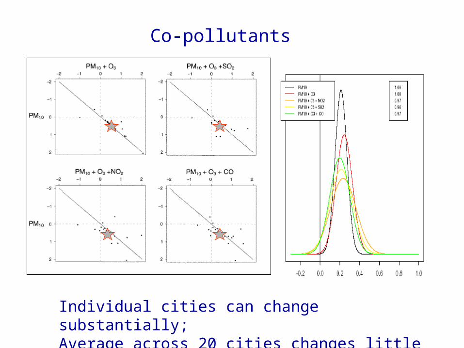
Co-pollutants

Individual cities can change substantially;Average across 20 cities changes little

3. Public Health Significance

• Harvesting idea – Only the very frail could possibly die from air

pollution– They would have died anyway in a few days– Air pollution, kills but causes only a trivial loss

of quality days of life• If true, we would expect associations only at

shorter time scales

Total Suspended Particles Mortality

Philadelphia Frequency Domain Decomposition

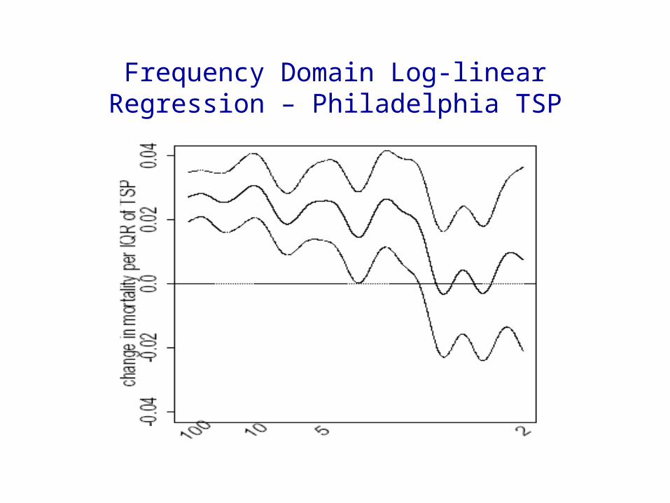
Frequency Domain Log-linear Regression – Philadelphia TSP

Frequency Band Relative Risk Estimates Pooled over 4 Cities

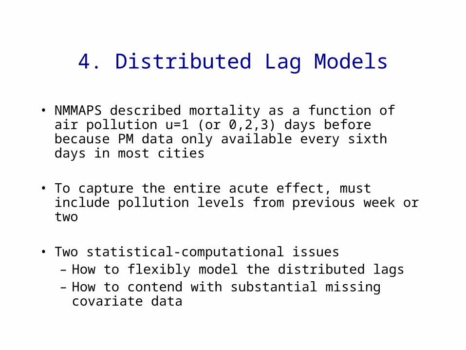
4. Distributed Lag Models

• NMMAPS described mortality as a function of air pollution u=1 (or 0,2,3) days before because PM data only available every sixth days in most cities

• To capture the entire acute effect, must include pollution levels from previous week or two

• Two statistical-computational issues– How to flexibly model the distributed lags– How to contend with substantial missing covariate data

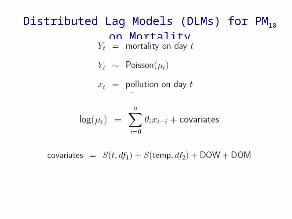
Distributed Lag Models (DLMs) for PM10 on Mortality

i

Effect of unit increase in PM10 7 days ago on today’s mortality

Distributed Lag Function

= ‘total effect’

i

i

0 2 4 6 8 10 12 14

-0.0002

-0.0001

0

0.0001

0.0002

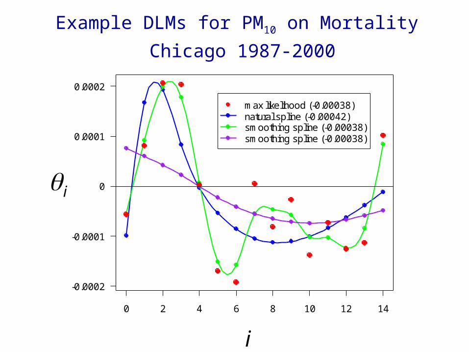
max likelihood (-0.00038)natural spline (-0.00042)smoothing spline (-0.00038)smoothing spline (-0.00038)

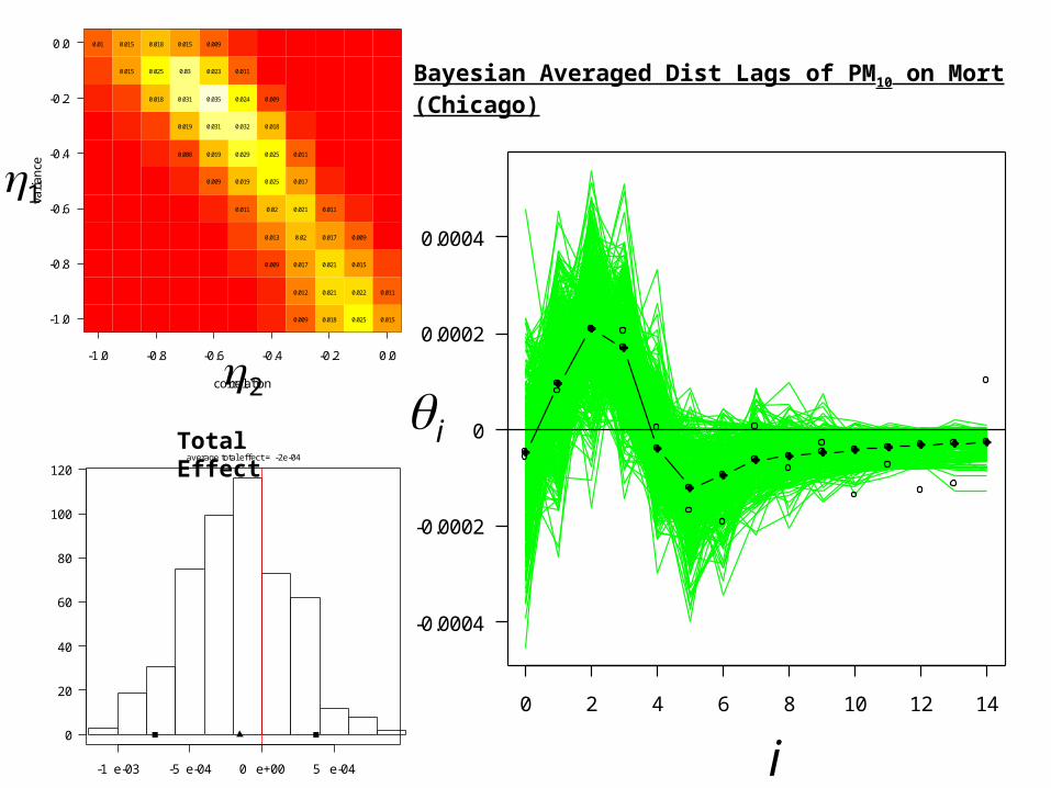
Example DLMs for PM10 on Mortality

Chicago 1987-2000

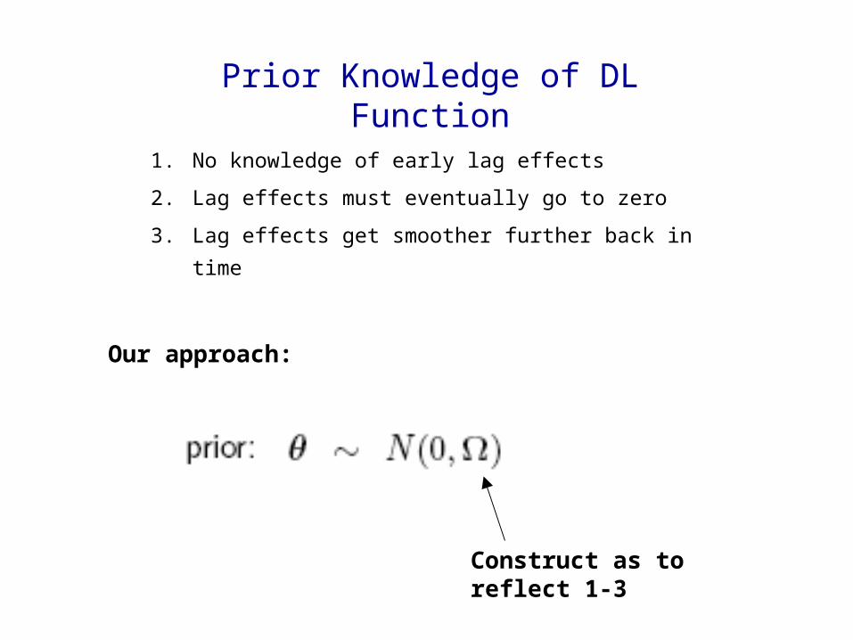
1. No knowledge of early lag effects

2. Lag effects must eventually go to zero

3. Lag effects get smoother further back in time

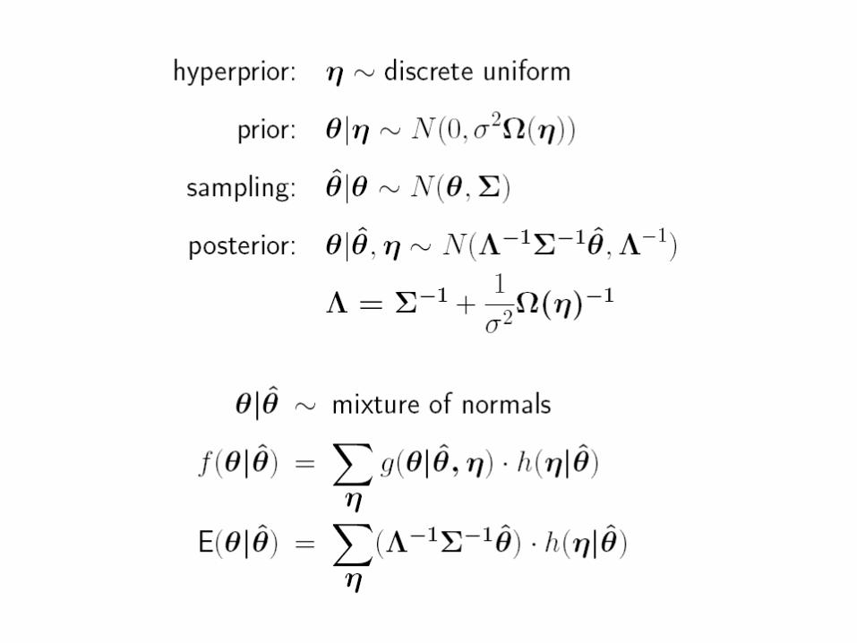
Prior Knowledge of DL Function

Our approach:

Construct as to reflect 1-3

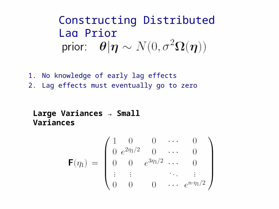
Constructing Distributed Lag Prior

1. No knowledge of early lag effects

2. Lag effects must eventually go to zero

Large Variances → Small Variances

3. Lag effects tend to zero smoothly

Uncorrelated → Correlated

-1.0 -0.8 -0.6 -0.4 -0.2 0.0

-1.0

-0.8

-0.6

-0.4

-0.2

0.0

correlation

vari

an

ce0.01

0.015

0.015

0.018

0.025

0.018

0.008

0.019

0.031

0.03

0.015

0.009

0.019

0.031

0.035

0.023

0.009

0.011

0.019

0.029

0.032

0.024

0.011

0.009

0.013

0.02

0.025

0.025

0.018

0.009

0.009

0.012

0.017

0.02

0.021

0.017

0.011

0.018

0.021

0.021

0.017

0.011

0.025

0.022

0.015

0.009

0.015

0.011

Bayesian Averaged Dist Lags of PM10 on Mort (Chicago)

-1 e-03 -5 e-04 0 e+00 5 e-04

0

20

40

60

80

100

120average total effect = -2e-04

Total Effect

1

2i

i0 2 4 6 8 10 12 14

-0.0004

-0.0002

0

0.0002

0.0004

-1.0 -0.8 -0.6 -0.4 -0.2 0.0

-1.0

-0.8

-0.6

-0.4

-0.2

0.0

correlation

vari

an

ce

0.031

0.028

0.025

0.021

0.017

0.013

0.009

0.031

0.028

0.024

0.02

0.015

0.011

0.03

0.027

0.022

0.018

0.014

0.01

0.029

0.025

0.02

0.016

0.012

0.028

0.023

0.018

0.013

0.009

0.025

0.02

0.015

0.011

0.022

0.016

0.012

0.018

0.013

0.009

0.015

0.01

0.014

0.009

0.016

0.011

0 2 4 6 8 10 12 14

-0.0005

0

0.0005

-5 e-04 0 e+00 5 e-04 1 e-03

0

20

40

60

80

100

average total effect = 2e-04

2

1

Total Effect

i

i

Bayesian Averaged Dist Lags of PM10 on Mort (Detroit)

Toward Reproducible Epidemiologic Reseach (RER)

• U.S. EPA setting national policy about air pollution based on acute and chronic disease studies – lots of $$ at stake

• Research conducted in the context of an adversarial debate about whether current levels of pollution cause mortality – credibility of epidemiologic evidence

Statistical Problem

Pollution signal embedded in

correlated “noise”

Convergence Problem

• NMMAPS estimated the city-specific relative rates using Generalized Additive Models (gam) in S-plus

• gam relies upon several parameters, four of which control the decision of when to declare convergence of the estimation algorithm

• 5 years into work, we discovered that the default parameters we used were too lax for our application

• In addition, Ramsey, et al discovered the gam under-estimates the standard errors of the relative rates estimates

Model Sensitivity: Relative Rate estimates for GAM (default and strict) versus GLM

Dominici, McDermott, Zeger, Samet AJE 2002

GAM (default) versus GLM estimates GAM(strict) versus GLM estimates

What Difference Did it Make?

The Press: The New York Times (June 2002)

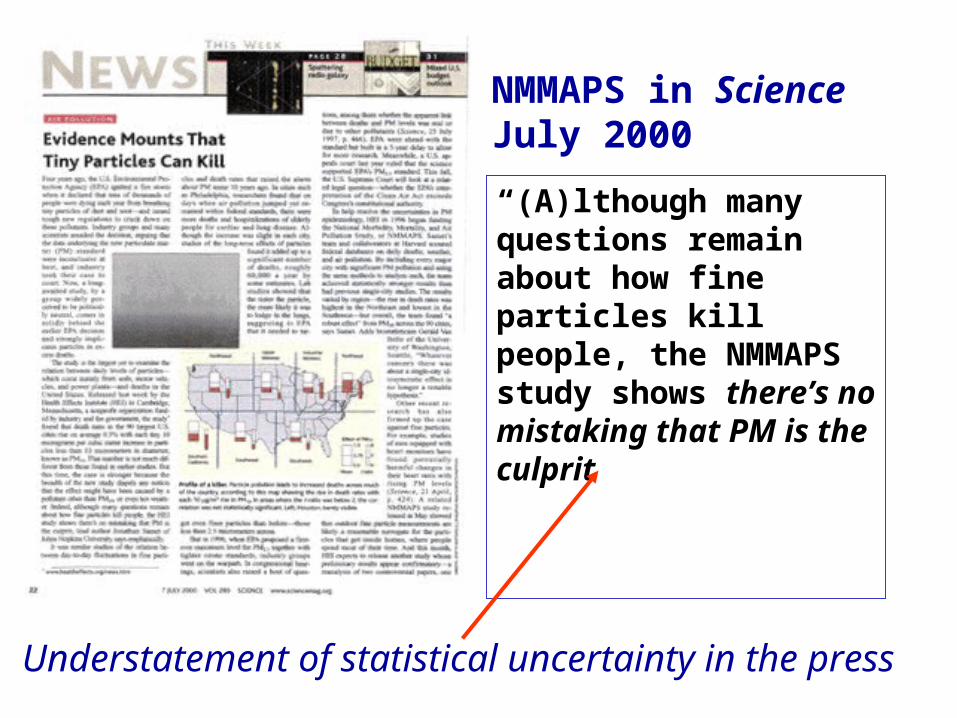
“(A)lthough many questions remain about how fine particles kill people, the NMMAPS study shows there’s no mistaking that PM is the culprit

NMMAPS in ScienceJuly 2000

Understatement of statistical uncertainty in the press

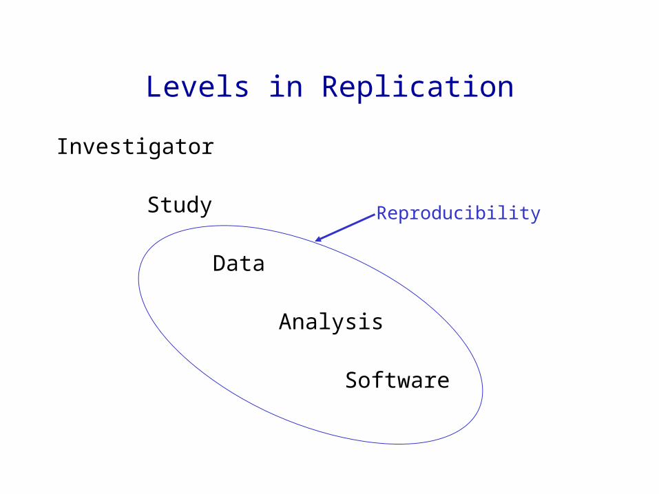
Levels in Replication

Investigator

Study

Data

Analysis

Software

Reproducibility

Toward Reproducibility in iHAPSS

• Post papers (tech reports) on iHAPSS web-site• Hyperlink main results in paper (tables, figures) to

– Statistical computing environment (R) with:• program that generates the results• datafile used by the program to generate the results

• Give user opportunity to alter the analyses – In this computing environment– In their own environment?

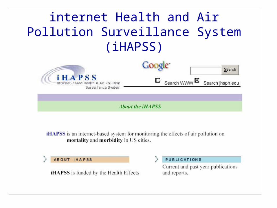
internet Health and Air Pollution Surveillance System (iHAPSS)

R as a Platform for Distributing Data

• Convenient online help system for documenting datasets

• Vignette system for more detailed descriptions of data or code

• Functions can be provided for handling data• Data can be delivered as a single unit/package,

rather than in separate (possibly unlinked) pieces

NMMAPSdata

• Preprocessing functions for setting up the database to reproduce recent NMMAPS findings

– basicNMMAPS: analysis of PM10 and mortality

– seasonal: estimating seasonally varying effects of PM10

– tempDLM: distributed lag models for temperature

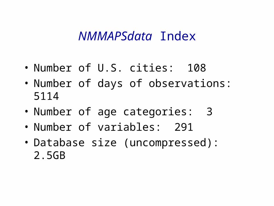
NMMAPSdata Index

• Number of U.S. cities: 108• Number of days of observations: 5114• Number of age categories: 3• Number of variables: 291• Database size (uncompressed): 2.5GB

Toward Reproducibility of Epidemiologic Research

• iHAPSS as a model• Journals require that published papers be

accompanied by programs/data necessary to reproduce their results

• Next steps to move the field in this direction

Main Points Once Again

• Reviewed the epidemiologic evidence for an association of particulate air pollution and mortality

– Cohort studies: RR=1.25 across range of exposures

– Time series studies:

• Mortality in space and time

– Summarize over time, then analyze in space

Main Points Once Again

• Value of Bayes estimates of maps of relative risks• Time-scale specific relative risks• Distributed lags models• Reproducible Epidemiologic Research

Science Statistics

Testimony on the EPA Proposed Decision on Particulate Matter

Suresh H. Moolgavkar, M.D., Ph.D.Professor of Epidemiology and Biostatistics, University of Washington

Industry Consultant “The proposed new regulations for particulate matter are based on the

assumption that the magnitude of the associations between these pollutants and adverse human health effects reported in some epidemiologic studies is predictive of the gains in human health that would accrue by lowering ambient concentrations. The evidence simply does not support this assumption. Briefly, the dearth of toxicological information, the absence of biological understanding of underlying mechanism, and the potential for uncontrolled confounding by co-pollutants currently preclude the conclusion that the particulate component of air pollution is causally associated with adverse effects on human health.”