Assessing the Existence of the J-Curve Effect in Bangladesh

The Bangladesh Development Studies

Vol. XXXII, June 2009, No. 2

Assessing the Existence of the J-Curve Effect in Bangladesh

by

RABEYA KHATOON*

MOHAMMAD MAHBUBUR RAHMAN*

This paper estimates the short run and long run impact of depreciation of Taka on trade balance in Bangladesh using cointegration techniques. The results support a positive influence of devaluation on trade balance both in the short and long run. The causal relationship between real exchange rate and trade balance is not robust, while the Granger test suggests a bidirectional causal relationship between devaluation and trade balance. The Sims test does not support the hypothesis that trade balance has influence on real exchange rate. On average, the declining segment of the ‘J-curve effect’ has not been evidenced for Bangladesh.

I. INTRODUCTION

Bangladesh economy is experiencing deficit in her balance of trade from the very beginning, which is the major source of her current account deficit, too. Import payments are two to three times higher than the export receipts generating an increasing trade deficit with increasing volume of exports and imports. Opening up the economy was initiated with the World Bank- IMF structural adjustment programmes of the 1980s with a belief that devaluation is necessary, if not sufficient, for reducing persistence trade deficit. Accordingly, Taka has been devalued frequently which was translated into real devaluation, though less than proportionately. Finally, the floating exchange rate regime was adopted in 2003.

The effectiveness of devaluation in improving trade balance depends on whether the Marshall-Learner condition holds, which states that devaluation will be successful in improving trade balance if the sum of the foreign price elasticity of demand for exports and the home country price elasticity of demand for imports is

* The authors are lecturer, Department of Economics, University of Dhaka and Graduate Student, Manchester University, UK respectively. They are grateful to Abdur Razzaque for his comments and suggestions on an earlier draft.


80

80

greater than unity. More specifically, devaluation reduces the volume of imports by raising the relative price of imports in domestic currency with price elastic import demand and increases export volume (more than the fall in the price of exports) by lowering the relative price of exports in foreign currency with price elastic foreign demand for exports. However, the short run and long run effects of devaluation can be different; the immediate impact of devaluation is the rise in imports value of the economy in local currency, while export value will remain unchanged and therefore, in the short run trade balance will deteriorate. Over a longer period of time, the export and import volumes will react to the changes in the relative prices and will result in an improvement in trade balance. Thus, a devaluation of the exchange rate will affect trade balance through both price and volume effects, the former effect of the devaluation leads to the deterioration of the trade balance, and the latter effect contributes to the improvement of trade balance––generating the famous ‘J-curve’ effect.

In the context of Bangladesh, the structuralist economist’s view rejects the hypothesis of positive impact of devaluation on trade balance on three considerations. First, imports of our country are subject to exchange controls and import licensing, thereby having an excess demand. Devaluation will only reduce this excess demand, not the actual import volume much. Second, Bangladesh’s imports are mainly necessary goods, machineries and raw materials and so import demand cannot be price elastic. Finally, for structural rigidities, supply elasticity of exports is low. However, the empirical findings are mixed––revealing price inelastic but income elastic export and import demand. And interestingly, the individual size of neither export price elasticity nor import price elasticity is high; still the price elasticity of demand for both export and import is high enough to satisfy the Marshall-Learner condition both in the short and long run for Bangladesh.

This paper applies a different methodology––the two-country imperfect substitution reduced form model––to estimate the trade balance equation for Bangladesh capturing both its short run and long run dynamics with the application of time series cointegration techniques. The estimation results provide support for the existence of cointegrating relationship between trade balance, real exchange rate and domestic and foreign income, and the conclusion is robust to the application of different cointegration techniques. The findings, on the whole, reflect that devaluation affects trade balance positively both in the short run and long run and thus implies that the falling part of the ‘J-curve’ is absent in Bangladesh.

II. LITERATURE REVIEW

A number of studies attempted to estimate short run and long run relationships between trade balance and exchange rate in different countries applying different

Khatoon & Rahman: Assessing the Existence of the J-Curve Effect

81

81

theoretical and methodological constructs. In this section, some of these studies are summarised in terms of their methodologies and findings.

In the case of the developed countries, the empirical findings of Rose and Yellen (1989) and Bahmani-Oskooee and Brooks (1999), with disaggregated bilateral trade data and Autoregressive Distributed Lag approach of Pesaran and Shin (1997), do not support for the existence of J-curve effect for USA, although the later study reports a long run positive relationship between devaluation and trade balance.

The study of Bahmani-Oskooee and Alse (1994) was to test the existence of cointegration between trade balance and exchange rate and for the J-curve effect in 41 developed and less developed countries with the Engle-Granger two-step procedure. The results indicated that for only fourteen countries the trade balance and real effective exchange rate are co-integrated. In the countries exhibiting cointegration, there was some evidence of the J-curve effect.

Zhang (1996) worked on the Chinese economy to test the direction of causality between exchange value of Renminbi and the price and quantity components of China’s trade balance by applying cointegration and Granger causality tests for the period 1991 to 1996 with monthly data. Their findings are not supportive to the existence of a J-curve, rather trade balance and each of its components Granger-cause changes in exchange rate.

Stučka (2004)’s investigation for J-curve effect for Croatia used a two-country, imperfect substitution model and estimated the short and long run trade balance equation as a function of domestic GDP, foreign GDP and real exchange rate. They applied the ARDL "delta" approach developed by Pesaran, Shin, and Smith (1996), the Bewley (1979) type ARDL model, and the ARDL instrumental variable approach described in Pesaran and Shin (1997) to test for cointegration and to estimate the impact of permanent exchange rate depreciation on the merchandise trade balance. Using quarterly data, the results of the study reported evidence of the J-curve effect in Croatia. The increase of the trade deficit as a consequence of the J-curve effect was estimated to be between 2.0 per cent and 3.3 per cent and the average length of the adverse effect of permanent depreciation was moderately above one quarter.

In relation to Bangladesh, there are various studies that estimated the import demand and export supply functions providing estimation of price and income elasticities of export and import to test the Marshall-Learner condition. The study of Rahman (1979) on the determinants of trade balance in Bangladesh for the periods 1959-68 and 1972-75 noted that in the earlier period, favourable price effect substantially reduced the impact of adverse quantity changes, whereas in the later


82

82

period both had unfavourable effects. The estimation of Islam and Hassan (2004) revealed income elastic and price inelastic aggregate import demand function.

However, in this line the most influential study for Bangladesh by Hossain (2000) used annual data for 1976-96 and applied cointegration techniques for estimating short and long run export supply and import demand functions. The estimated price elasticities were then used to test the Marshall-Learner condition and found that the condition holds for Bangladesh both in the short run and long run, implying that devaluation effectively improves trade balance in Bangladesh.

On the whole, there are mixed evidences for countries and estimation techniques on the existence of J-curve effect and therefore, it cannot be termed as an empirical regularity.

III.THEORETICAL MODEL

In this paper, the "two-country" imperfect substitutes model is used to specify the trade balance equation as was used by Stučka (2004) in a similar study on Croatia. Key assumptions of the model are that neither imports nor exports are perfect substitutes for domestic goods, so that finite elasticities for demand and supply can be estimated for most traded goods. The volume of imports demanded

domestically, dM , and the quantity of imports demanded by the rest of the world, *dM , are given by equations (1) and (2):

0P/dM0,mP/dM0,Y/dMP),,mP(Y,1fdM (1)

0*P/*dM,0*

mP/*dM,0e*Y/*

dM),*P,*mP,e*Y(2f*

dM (2)

where Y is domestic income, Pm the domestic currency price paid by domestic importers and P denotes the overall domestic price level, i.e. the price of all

domestically produced goods. In equation (2), *Y represents foreign income, e the

exchange rate expressed as the domestic currency price of foreign exchange, *mP

denotes the foreign currency price paid by domestic importers and *P the overall foreign price level. In other words, the demanded quantity is a function of the level of money income in the importing region, the imported goods' own price and the price of domestic substitutes. The use of aggregated data allows the assumption that inferior goods or domestic complements are excluded. This implies that domestic income and foreign income elasticity and the cross-price elasticities of demand are assumed to be positive and the own-price elasticities to be negative. Furthermore, it should be noted that the demand variables are represented only by current income rather then permanent and transitory income.


83

83

Usually in such models the demand function is assumed to be homogeneous of degree zero reflecting that the consumer does not suffer from money illusion–– demand will remain constant when doubling money income and prices. Hence, this homogeneity assumption is expressed by dividing the explanatory variables on the right hand side by P. In this way, arguments of the demand function are expressed in real terms––real income and relative prices of import to domestically produced goods. These modifications allow us to re-write equations (1) and (2) as

P/mPmRP,P/YrY;0mRP/dM,0rY/dM),mRP,rY(1fdM (3)

*P/*mP*

mRP,*P/*Y*rY;0*

mRP/*dM,0*

rY/*dM),*

mRP,*rY(2f*

dM (4)

Since the relative price of imports is equivalent to the foreign currency price of

foreign exports adjusted for the exchange rate we may define the relative price of imports as

*x

**x

**x

**xmm QpP/QPPP/PePP/ePP/PRP (5)

where *xp represents real foreign currency price of exports, while P/ePQ * ,

denotes the real exchange rate defined in such a way that an increase in Q refers to a depreciation of the domestic currency.

Finally, the rest of the world export supply function, and the quantity of exports domestically supplied to the rest of the world are given in equations (6) and (7):

)P,P(fX x3s (6)

)P,(PfX **x4

*s (7)

where xP is the domestic currency price received by domestic exporters and

vice versa.

The equilibrium demand and supply conditions for both regions are determined by conditions (8) and (9):

eXM *sd (8)

s*d XM (9)

Hence, the trade balance

d*x

*dx MQpMpTB (10)


84

84

and solving for levels of domestic exports and imports as well as the relative price level of imports as a function of the real exchange rate we obtain the partial reduced form of the domestic trade balance in (11):

0Q/TB,0Y/TB,0Y/TB,)Q,Y,Y(fTB *rr

*rr (11)

Hence, we expect real foreign income and real exchange rate to be positively related to the trade balance and domestic income negatively related to the trade balance.

IV. DATA DESCRIPTION

IV.1 Technical Data Description

This section describes the sources of data, the estimation methodology of the variables and the potential problems associated with the data.

The estimation period is from 1972 (the starting of Bangladesh period) to 2006 (the recent year up to which all the required information are available). Although short run and long run effects are better captured by quarterly data, here yearly data is taken since GDP data is only available on yearly basis. The data is taken from the International Financial Statistics (IFS) and The Direction of Trade Statistics (DOTS), both published by International Monetary Fund (IMF).

The variable Trade Balance of Bangladesh (TB) is estimated as the ratio of Export to Import to avoid the problem with nominal and real estimates and to have positive values so that logarithmic form can be used for estimation.

Domestic GDP (GDPD) is the measure of index of Bangladesh’s GDP volume with 2000 as base. Foreign GDP (GDPF) is estimated as the trade weighted average of the index of GDP volume of twenty trading partners of Bangladesh–Australia, Belgium, Canada, China-Hong Kong, China-Mainland, Germany, India, Indonesia, Italy, Japan, Korea, Kuwait, Malaysia, Netherlands, Saudi Arabia, Singapore, Spain, Thailand, UK and USA––accounting for 65 to 70 per cent of our total trade.

The Estimation Methodology of the Variable Real Exchange Rate (RER)

According to the trade theory definition, Real Exchange Rate (RER) is the ratio of price of tradables ( TP ) to price of non-tradables ( NTP ). However, the operational

definition of RER suggests using foreign wholesale price index ( fWPI ) as a proxy

for TP and domestic consumer price index ( dCPI ) for NTP so that the bilateral

RER equation becomes:

)CPI/WPI(ERER df (12) where, E = Nominal Exchange Rate.


85

85

In usual practice, the multilateral Real Exchange Rate (RER) using trade theory definition is constructed considering the important trading partners with weights ( i ) equal to the share of each partner in the country’s total trade:

dt

fitiitt CPI/WPI(ERER with 1 i (13)

where, trade share of the partners are taken as average share for a longer period.

Referring to the case of Bangladesh, due to the unavailability of data on the WPI and exchange rate of Taka against the currencies of each of her trading partners, the computation of RER in this paper is based on the following modified equation:

dt

$i

fiti

$tt CPIr/CPIERER with 1 i (14)

Where, $tE = The exchange rate of Bangladeshi Taka against US$

i = ith country’s share in the total trade of Bangladesh (period average 1997-2006), i = 1, 2, 3…20. f

itCPI = ith country’s Consumer Price Index

$ir = ith country’s exchange rate against US$

dtCPI = Bangladesh’s Consumer Price Index.

Finally, the estimated RER series is adjusted as an index with base year 2000.

The variable exchange rate, as defined here, reflects devaluation of Taka with an increase in value and vice versa. All the four variables––TB, GDPD, GDPF and RER––are taken in logarithmic form for estimation.

However, it should be noted that the use of CPI instead of WPI would not be a source of much variation in RER, since WPI and CPI are usually highly correlated. Data on the exchange rates of the European Union countries against US$ exhibit a jump in 1999 with the introduction of Euro. Therefore, to maintain continuity, extrapolation is done for 1999-2006 for those countries applying general forecasting methodology.

IV.2 Econometric Characteristics of Data

In time series econometrics, existence of a valid long run relationship among the variables depends on whether the variables are stationary or not. If the variables are non-stationary, the OLS estimates may lead to spurious regression problems with the t and F tests being non-standard. The problem with non-stationary time series may arise if the variables are generated either by trend stationary process (TSP) or by difference stationary process (DSP). The TSP variables are made


86

86

stationary through de-trending them and the DSP variables need to be differenced until they are stationary. The Unit Root tests are the formal tests to determine whether the data generating process is TSP or DSP.

In this section, we will examine the stationarity of the four variables (LTB, LGDPD, LGDPF and LRER) by applying the Augmented Dickey Fuller (ADF) test and Phillips-Perron (1988) tests of unit root.

The popular tests for unit root are the Dickey Fuller (DF) and ADF tests. The ADF test is a modification of the DF test and involves augmenting the equation for the DF test by lagged values of the dependent variables. This is done to ensure that the error process in the estimating equation is residually uncorrelated. Therefore, the ADF version of the test is based on the equation-

t1t1tt eYTY)1(Y (15)

The t-ratio on (ρ-1) provides the ADF test statistic. However, both the estimated t-ratios for the DF and ADF tests are non-standard requiring more demanding critical values to compare to infer about the stationarity of the variables. Therefore, we have to use the critical values provided by Dickey and Fuller.

Besides, the Phillips-Perron (1988) test for unit root generalises the results of equation 15 in the case when the error term et is serially correlated and possibly heteroskedastic as well, i.e,

0j

jtjtt )L(e

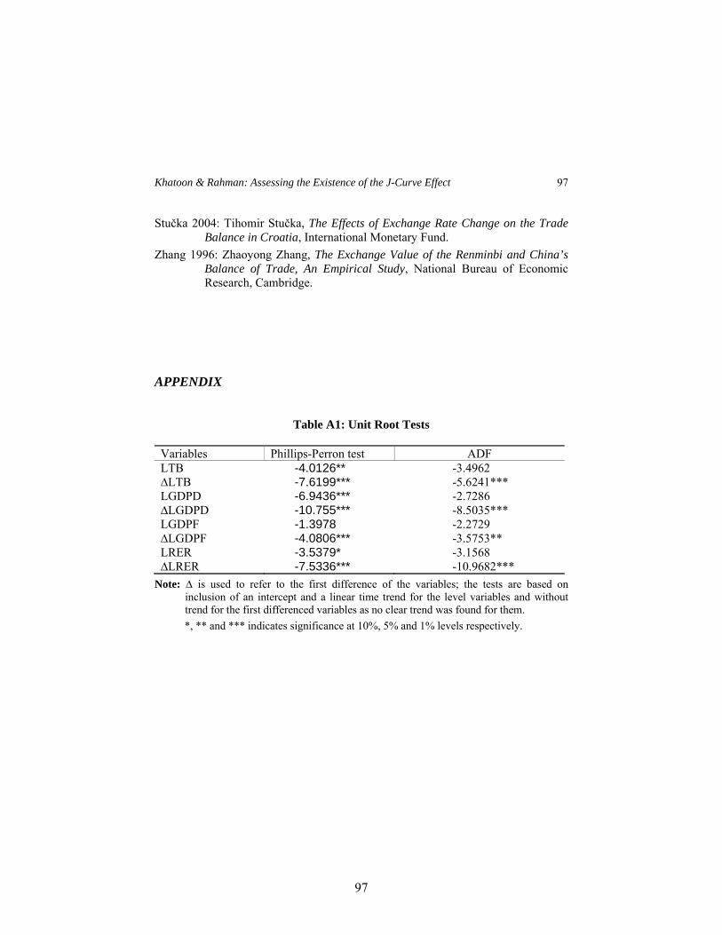
Table A1 reports the results of ADF and Phillips-Perron tests for the four variables and their first differences to determine the order of integration of the variables. Following Engle and Granger (1987) a time series is said to be integrated of order d [usually denoted as ~I (d)] with d is the number of times the series needs to be differenced in order to become stationary.

Table A1 represents that for the level variables, the absolute values of the ADF test statistics are less than the critical values, implying that the variables are non-stationary on their level. On the other hand, both ADF and Phillips-Perron test statistics for all the variables on their first differences imply stationarity. Therefore, it is reasonable to use the first differenced forms of the variables for estimation to ensure stationarity. Again, in the case of small sample, Hall (1986) suggests the inspection of the autocorrelation function and correlogram as an important tool in determining whether the variables are stationary or not. The sample autocorrelation function for any variable at any lag k is defined by the ratio of covariance at lag k divided by variance. When the estimated autocorrelation coefficients at different lags are plotted against k, sample correlogram is obtained. For non-stationary


87

87

variables, correlograms die down slowly giving rise to either a secular declining or a constant trend in the graph of autocorrelation coefficients while in the case of stationary variables they damp down almost instantly and then show random movement. In this paper, the integrating orders of the variables are further tested with the correlograms presented in Figure A.1 that supports that our variables of interest LTB, LGDPD, LGDPF, and LRER are integrated of order 1 (I (1)) at their levels and therefore stationary with first differences.

Finally, Figure 1 gives us a scatter plot of the level and first difference of the two variables of our interest, LTB and LRER. A positive relationship between the real exchange rate (LRER) and trade balance (LTB) is shown in both the level and the first differenced observations, implying that devaluation of exchange rate has a positive influence on trade balance both in the short and long run. However, we must check, first of all, whether a valid long run relationship among them exists or not through cointegration analysis before making such conclusions.

Figure 1: Scatter Plot of LTB and LRER Scatter plot of LTB and LRER

Scatter plot of DLTB and DLRER

V. ECONOMETRIC ESTIMATION

Once we have identified variables as non-stationary, the only way to infer about the long run relationship is to apply some cointegration techniques. In this paper we have applied the Johansen Procedure of cointegration and short run dynamics are analysed using error correction model. In this connection, Vector Error Correction (VEC) model is also used.1

1 Similar results can be found using the Engle-Granger procedure and the Unrestricted Error Correction Model both in the case of long run and short run behaviours and therefore are not reported here.

-1.6

-1.4

-1.2

-1

-0.8

-0.6

-0.4

-0.2

0

0 1 2 3 4 5

LR ER

-0.6

-0.4

-0.2

0

0.2

0.4

0.6

0.8

-0.4 -0.3 -0.2 -0.1 0 0.1 0.2

D LR ER


88

88

The Johansen Procedure

The Johansen procedure can estimate multiple cointegrating vectors. This approach works with the estimation of Vector of Autoregression (VAR) of the form:

tt1t

1

1i

it uXXX

(16)

where tX is a column vector of n endogenous variables, Π and Πi are n by n

matrices of unknown parameters, and ut is an error term. All long-run information about the relationship between variables is contained in the impact matrix Π. When the matrix Π has full column rank, it implies that all variables in X are stationary. When the matrix Π has zero rank, the system is a traditional first-differenced VAR involving no long-run elements. However, when the rank of Π is intermediate or 0 < rank (Π) = r < n, there exist r cointegrating vectors that make the linear combinations of tX become stationary or cointegrated. Two tests for cointegration,

provided by Johansen and Juselius, are the Trace test and the Maximal Eigen value test.

At first the autoregressive order of VAR is to be chosen. Based on the comparison of adjusted R2 values, Akaike Information Criterion and Schwarz Bayesian Criterion among the VAR order 1, 2, 3 and 4 estimation results, VAR order 2 is chosen to be the appropriate. The results are shown in Table I.

TABLE I JOHANSEN TEST FOR COINTEGRATION

Maximal Eigenvalue Test Null Alternative Statistic 95% Critical Value Conclusion r = 0 r<= 1 r<= 2 r<= 3

r = 1 r = 2 r = 3 r = 4

59.5493 14.0213 13.1107

1.7056

27.4200 21.1200 14.8800

8.0700

Single cointegrating vector

Trace Test

Null Alternative Statistic 95% Critical Value Conclusion r = 0 r<= 1 r<= 2 r<= 3

r>= 1 r>= 2 r>= 3 r = 4

88.3868 28.8375 14.8163

1.7056

48.8800 31.5400 17.8600

8.0700

Single cointegrating vector

Cointegrating Vector: LTB LGDPD LGDPF LRER 1.00 -2.7704 1.7913 3.3054


89

89

The results presented in Table V show that the null hypothesis of no cointegration is strongly rejected in both the tests and the tests suggest the existence of one cointegrating vector. It should be noted here that the estimation is without an intercept term, inclusion of which is theoretically meaningless. The results suggest the existence of a positive long run relationship of trade balance with devaluation of exchange rate and foreign income, and a negative relationship with domestic income.

Short Run Dynamics under Johansen Procedure

Short run dynamics are estimated by inserting the one period lagged residual obtained from the cointegrating relationship in the general short run model. Table II gives the estimation results of the error correction model obtained using the “general to specific” methodology.

TABLE II SHORT RUN ERROR CORRECTION MODEL UNDER JOHANSEN PROCEDURE

Variables Estimated coefficients (t-ratio)

Intercept -5.37772 (-5.180)

∆LGDPD 3.29999 (2.806)

∆LGDPD (-1) 3.54527 (3.048)

∆LGDPF 4.25985 (3.146)

∆LRER 1.25018 (3.840)

∆LRER (-1) 0.49463 (2.408)

Adjustment (Error Correction Term) -0.42428 (-5.055)

Adjusted R2 0.69881

Serial Correlation[χ2 (1)] 0.4149

Heteroscedasticity [χ2(1)] 10.6806

Normality [χ2 (2)] 1.2651

Reset [χ2 (1)] 0.9765

Surprisingly, the short run exchange rate elasticity of trade balance is also positive, as reported in Table II, implying that devaluation of currency improves trade balance even in the short run in Bangladesh. Additionally, the estimates reflect significant positive influence of domestic GDP as well as foreign GDP over trade balance in the short run. The error correction term indicates a quick adjustment towards long run equilibrium if any short run deviation occurs.


90

90

Vector Error Correction Model Approach

Another approach to deal with the short run dynamics of time series models is to apply vector error correction (VEC) model––a restricted VAR that has cointegration restrictions built into the specification, so that it is designed for use with nonstationary series that are known to be cointegrated. The VEC specification restricts the long-run behaviour of the endogenous variables to converge to their cointegrating relationships while allowing a wide range of short-run dynamics. The cointegration term is known as the error correction term since the deviation from long-run equilibrium is corrected gradually through a series of partial short-run adjustments.

Based on the analysis above, our specification has one cointegrating vector and that is used to estimate short-run dynamics with VEC modeling technique. However, only the equation with first-differenced Trade Balance (LTB) as the dependent variable serves our interest and is economically meaningful and therefore is reported here. As Table III reports, the short run response of trade balance to real exchange rate is positive and significant. The error correction term is rightly signed, though significant at only 9 per cent level.

TABLE III

SHORT RUN ERROR CORRECTION MODEL UNDER VECM

Variables Estimated coefficients (t-ratio) Intercept -0.0902 (-1.314) LTB(-1) -0.3045 (-2.255) LRER(-1) 0.8046 (-3.702) LGDPF(-1) 1.0955 (-0.731) LGDPD(-1) 0.9993 (-1.421) Adjustment (Error Correction Term) -0.1156 (-1.752) Adjusted R2 0.4783 Serial Correlation[F(2,25)] 0.1308 Heteroscedasticity [F(10,16)] 0.6606 Normality [χ2 (2)] 0.2183 Reset [F(1,26)] 6.1937

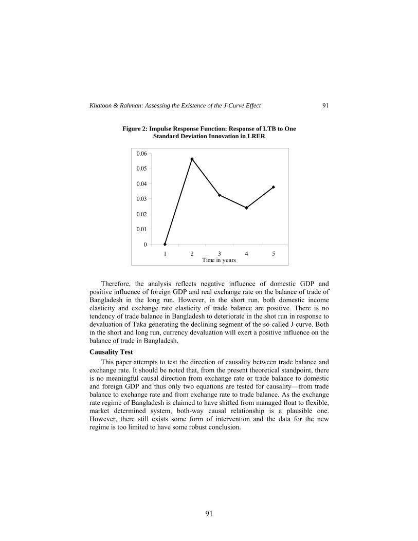
Figure 2 gives the impulse response function estimated from the VEC model. For one standard deviation innovation in log real exchange rate, there is positive response of log trade balance with a sharp increase in the first year and the reduction followed by increase again. This indicates that the initial falling part of the conventional J-curve is absent for Bangladesh.


91

91

Figure 2: Impulse Response Function: Response of LTB to One Standard Deviation Innovation in LRER

Therefore, the analysis reflects negative influence of domestic GDP and positive influence of foreign GDP and real exchange rate on the balance of trade of Bangladesh in the long run. However, in the short run, both domestic income elasticity and exchange rate elasticity of trade balance are positive. There is no tendency of trade balance in Bangladesh to deteriorate in the shot run in response to devaluation of Taka generating the declining segment of the so-called J-curve. Both in the short and long run, currency devaluation will exert a positive influence on the balance of trade in Bangladesh.

Causality Test

This paper attempts to test the direction of causality between trade balance and exchange rate. It should be noted that, from the present theoretical standpoint, there is no meaningful causal direction from exchange rate or trade balance to domestic and foreign GDP and thus only two equations are tested for causality––from trade balance to exchange rate and from exchange rate to trade balance. As the exchange rate regime of Bangladesh is claimed to have shifted from managed float to flexible, market determined system, both-way causal relationship is a plausible one. However, there still exists some form of intervention and the data for the new regime is too limited to have some robust conclusion.

0

0.01

0.02

0.03

0.04

0.05

0.06

1 2 3 4 5Time in years


92

92

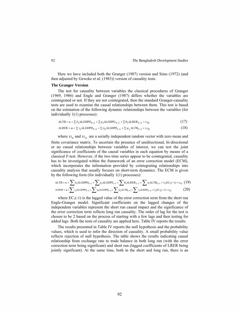
Here we have included both the Granger (1987) version and Sims (1972) (and then adjusted by Geweke et al. (1983)) version of causality tests.

The Granger Version

The test for causality between variables the classical procedures of Granger (1969, 1986) and Engle and Granger (1987) differs whether the variables are cointegrated or not. If they are not cointegrated, then the standard Granger-causality tests are used to examine the causal relationships between them. This test is based on the estimation of the following dynamic relationships between the variables (for individually 1(1) processes):

t1itLRERiitLGDPGiitLGDPDiLTB (17)

t2itLTBiitLGDPFiitLGDPDiLRER (18)

where t1 and t2 are a serially independent random vector with zero mean and

finite covariance matrix. To ascertain the presence of unidirectional, bi-directional or no causal relationships between variables of interest, we can test the joint significance of coefficients of the causal variables in each equation by means of a classical F-test. However, if the two time series appear to be cointegrated, causality has to be investigated within the framework of an error correction model (ECM), which incorporates the information provided by cointegrating relationships into causality analysis that usually focuses on short-term dynamics. The ECM is given by the following form (for individually 1(1) processes):

t111itiitiitiiti )1(ECLTBLRERLGDPFLGDPDLTB (19)

t2)1(2EC2itLRERiitLTBiitLGDPFiitLGDPDiLRER (20)

where EC1(-1) is the lagged value of the error correction term from the short run Engle-Granger model. Significant coefficients on the lagged changes of the independent variables represent the short run causal impact and the significance of the error correction term reflects long run causality. The order of lag for the test is chosen to be 2 based on the process of starting with a few lags and then testing for added lags. Both the tests of causality are applied here. Table IV reports the results.

The results presented in Table IV reports the null hypothesis and the probability values, which is used to infer the direction of causality. A small probability value reflects rejection of null hypothesis. The table shows the results indicating causal relationship from exchange rate to trade balance in both long run (with the error correction term being significant) and short run (lagged coefficients of LRER being jointly significant). At the same time, both in the short and long run, there is an


93

93

indication of causal relationship from trade balance and foreign GDP to RER with the significant coefficients and error term in LRER equation.

TABLE IV CAUSALITY TEST WITH COINTEGRATING RELATIONSHIP

Causality ∆LTB ∆LGDPD ∆LGDPF ∆LRER Test of joint

significance Error correction term

∆LTB equation LTB Null Hypothesis P-value

-

δi=0, for all i (0.397)

ρi=0, for all i (0.200)

θi=0, for all i (0.063)

δi=ρi=θi=0, for all i (0.010)

λ1=0 (0.014)

∆LRER equation LRER Null Hypothesis P-value

ψi=0, for all i (0.047)

γi=0, for all i (0.325)

ηi=0, for all i (0.002)

-

ψi=γi=ηi=0, for all i (0.005)

λ2=0 (0.072)

The Sims Version

Another form of causality test proposed by Sims (1972) and then modified by Geweke, Messe and Dent (1983) is considered here to test the robustness of the results. The difference between the Sims test and the Granger test is that instead of considering the differenced forms of the variables, Sims test regress level dependent variable on lagged, level and lead independent variable(s) of interest and test for the joint significance of the coefficients of the lead variables. Formally, considering the following equations:

t1LGDPFLGDPD

1j

jtLRERjb

0j

jtLRERja1tLTB

(21)

t2LGDPFLGDPD1j

jtLTBjd0j

jtLTBjc2tLRER

(22)

where ja , jb and jc , jd are defined as population projection coefficients, i.e.,

the values for which 01 st LRERE and 02 st LTBE for all t and s, then

LTB fails to cause LRER if and only if jb = 0 and LRER fails to cause LTB if and

only if jd = 0, for all j=1,2,3,………. .


94

94

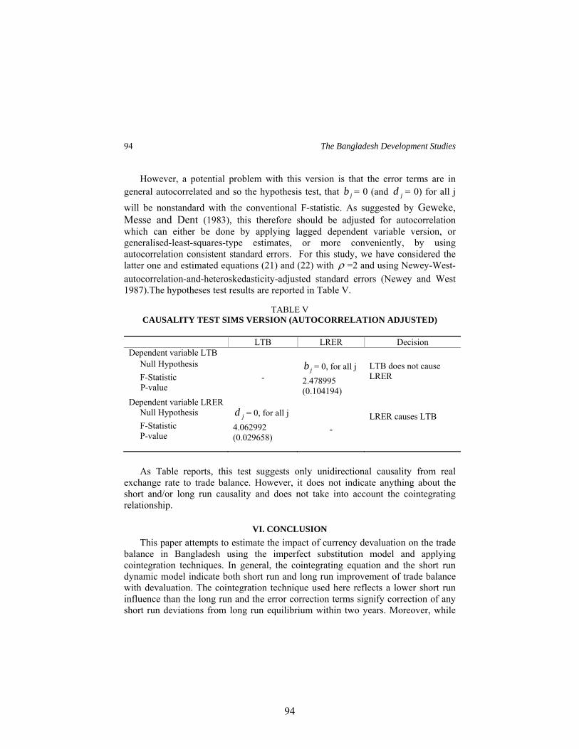
However, a potential problem with this version is that the error terms are in general autocorrelated and so the hypothesis test, that jb = 0 (and jd = 0) for all j

will be nonstandard with the conventional F-statistic. As suggested by Geweke, Messe and Dent (1983), this therefore should be adjusted for autocorrelation which can either be done by applying lagged dependent variable version, or generalised-least-squares-type estimates, or more conveniently, by using autocorrelation consistent standard errors. For this study, we have considered the latter one and estimated equations (21) and (22) with =2 and using Newey-West-autocorrelation-and-heteroskedasticity-adjusted standard errors (Newey and West 1987).The hypotheses test results are reported in Table V.

TABLE V CAUSALITY TEST SIMS VERSION (AUTOCORRELATION ADJUSTED)

LTB LRER Decision Dependent variable LTB

Null Hypothesis

F-Statistic P-value

-

jb = 0, for all j

2.478995 (0.104194)

LTB does not cause LRER

Dependent variable LRER Null Hypothesis

F-Statistic P-value

jd = 0, for all j

4.062992 (0.029658)

-

LRER causes LTB

As Table reports, this test suggests only unidirectional causality from real exchange rate to trade balance. However, it does not indicate anything about the short and/or long run causality and does not take into account the cointegrating relationship.

VI. CONCLUSION

This paper attempts to estimate the impact of currency devaluation on the trade balance in Bangladesh using the imperfect substitution model and applying cointegration techniques. In general, the cointegrating equation and the short run dynamic model indicate both short run and long run improvement of trade balance with devaluation. The cointegration technique used here reflects a lower short run influence than the long run and the error correction terms signify correction of any short run deviations from long run equilibrium within two years. Moreover, while


95

95

the Granger causality test provides support to the existence of both short run and long run bidirectional causal relationship between devaluation and trade balance, the Geweke, Messe and Dent (1983) proposed modified Sims (1972) test supports only causal relationship from real exchange rate to trade balance, not vice versa.

Finally, it should be noted that the estimation results are for the aggregate trade balance of Bangladesh and with trade-weighted averaged real exchange rate of her twenty major trading partners. In other words, the trade balance response incorporates the asymmetric response of trade flows to exchange rate changes across the twenty countries. Hence, the non-existence of ‘J-curve’ effect on an aggregated level means that, on average, it does not hold for Bangladesh, and in the disaggregated level it could still be valid for some of the countries. Moreover, the use of annual data model extends the short run time span, whereas a quarterly model could have captured the true short run dynamics. On the whole, the policy conclusion stems from our analysis is that currency devaluation improves trade balance in Bangladesh.

REFERENCES

Bahmani-Oskoee and Janardhanan 1994: Mohsen Bahmani-Oskoee and Janardhanan Alse, “Short-Run Versus Long-Run Effects of Devaluation: Error-Correction Modeling and Cointegration,” Eastern Economic Journal, 20 (4):453– 464.

_____ and Brooks 1999: Mohsen Bahmani-Oskoee and Taggert J. Brooks, “Bilateral J-curve Between U.S. and Her Trading Partners,” Weltwirtschaftliches Archiv, 135 (1):156 – 165.

Bewley 1979: Ronald Bewley, “The Direct Estimation of The Equilibrium Response in a Linear Dynamic Model,” Economics Letters 3:357–361.

Edwards 1988: Sebastian Edwards, Exchange Rate Misalignment in Developing Countries, World Bank, Washington, D.C.

Engel and Granger 1987: R.F. Engel and C.W.J. Granger, “Cointegration and Error-correction Representation, Estimation and Testing;” Econometrica, 55: 251-76.

Geweke, Messe and Dent 1983: J.Geweke, R.Messe and W.Dent, “Comparing Alternative Tests of Causality in Temporal Systems,” Journal of Econometrics, 21: 161-194.

Granger 1969: C.W.J. Granger, “Investigating Causal Relations by Econometric Models and Cross-spectral Methods,” Econometrics, 37: 424-438.


96

96

_____1986: Clive W.J. Granger, “Developments in the Study of Cointegrated Economic Variables,” Oxford Bulletin of Economics and Statistics 48: 213-228.

Gujarati 2002-03: Damodar N. Gujarati, Basic Econometrics, McGraw-Hill International Edition.

Hall 1986: S. Hall, “An Application of the Granger and Engle Two-Step Estimation Procedure to United Kingdom Aggregate Wage Data,” Oxford Bulletin of Economics and Statistics, 48 (3): 229-240.

Harris 1995: R.I.D. Harris, Using Cointegration Analysis in Econometric Modelling, Prentice Hall.

Hossain 2000: Akhtar Hossain, Exchange Rates, Capital Flows and International Trade: A Case of Bangladesh, University Press Limited.

IMF: Direction of Trade Statistics ( Various Issues).

_____: International Financial Statistics (Various Issues).

Islam and Hassan 2004: Anisul M. Islam & M. Kabir Hassan, “An Econometric Estimation of the Aggregate Import Demand Function for Bangladesh: Some Further Results,” Applied Economics Letters, 11.

Newey and West 1987: Whitney K. Newey and Kenneth D. West, “A Simple Positive Semi-definite, Heteroskedasticity and Autocorrelation Consistent Covariance Matrix,” Econometrica, 55: 703-8.

Pesaran and Shin 1997: Hashem Pesaran and Yongcheol Shin, “An Autoregressive Distributed Lag Modelling Approach to Cointegration Analysis,” DAE Working Papers Amalgamated Series, University of Cambridge.

_____ and Smith 1996: Hashem Pesaran, Yongcheol Shin, and Ron J. Smith, “Testing for the Existence of a Long-Run Relationship,” DAE Working Papers Amalgamated Series, No. 9622, University of Cambridge

Phillips and Perron 1988: Peter C. B. Phillips and Pierre Perron, “Testing For a Unit Root in Time Series Regression,” Biometrika, 75 (2): 335-346.

Rahman 1979: Sultan H. Rahman, “The Determinants of Change in Trade Balance: Some Estimates for Bangladesh, 1959/60-1974/75,” Bangladesh Develop-ment Studies, VII (2).

Rose and Yellen 1989: Andrew Rose and Janet L. Yellen, “Is There a J-curve?” Journal of Monetary Economics, 24:53-68.

Sims 1972: C. A Sims, “Money, Income, and Causality,” The American Economic Review, 62 (4): 540-552.


97

97

Stučka 2004: Tihomir Stučka, The Effects of Exchange Rate Change on the Trade Balance in Croatia, International Monetary Fund.

Zhang 1996: Zhaoyong Zhang, The Exchange Value of the Renminbi and China’s Balance of Trade, An Empirical Study, National Bureau of Economic Research, Cambridge.

APPENDIX

Table A1: Unit Root Tests Variables Phillips-Perron test ADF LTB -4.0126** -3.4962 ∆LTB -7.6199*** -5.6241*** LGDPD -6.9436*** -2.7286 ∆LGDPD -10.755*** -8.5035*** LGDPF -1.3978 -2.2729 ∆LGDPF -4.0806*** -3.5753** LRER -3.5379* -3.1568 ∆LRER -7.5336*** -10.9682***

Note: ∆ is used to refer to the first difference of the variables; the tests are based on inclusion of an intercept and a linear time trend for the level variables and without trend for the first differenced variables as no clear trend was found for them.

*, ** and *** indicates significance at 10%, 5% and 1% levels respectively.

Figure A1: Correlograms

LRER DLRER

-0.4-0.2

00.20.40.60.8

1

1 2 3 4 5 6 7 8 9 10 11Order of lags

-0.4

-0.2

0

0.2

0.4

1 2 3 4 5 6 7 8 9 10 11Order of lags

LTB DLTB

-0.4

-0.2

0

0.2

0.4

0.6

0.8

1

1 2 3 4 5 6 7 8 9 10 11Order of lags

-0.4-0.3-0.2-0.1

00.10.20.30.4

1 2 3 4 5 6 7 8 9 10 11

Order of lags

LGDPD DLGDPD

-0.4

-0.2

0

0.2

0.4

0.6

0.8

1

1 2 3 4 5 6 7 8 9 10 11

Order of lags

-0.4-0.3-0.2-0.1

00.10.20.30.4

1 2 3 4 5 6 7 8 9 10 11

Order of lags

LGDPF DLGDPF

-0.4-0.2

00.20.40.60.8

1

1 2 3 4 5 6 7 8 9 10 11

Order of lags

-0.4

-0.2

0

0.2

0.4

1 2 3 4 5 6 7 8 9 10 11

Order of lags

Assessing the Existence of the J-Curve Effect in Bangladesh

Documents

Transcript of Assessing the Existence of the J-Curve Effect in Bangladesh