Combining Symbolic Simulation and Interval Arithmetic for the Verification of AMS Designs

Nausicaa onboard software MassimilianoVasile, Muro Massari, Giovanni Giardini Department of Aerospace Engineering, Politecnico di Milano
ESA ITI contract 18693/04/NL/MV
1
\ASSESSING THE ACCURACY OF INTERVAL
ARITHMETIC ESTIMATES IN SPACE FLIGHT MECHANICS
ASSESSING THE ACCURACY OF INTERVAL
ARITHMETIC ESTIMATES IN SPACE FLIGHT MECHANICS Contract number 18851/05
Senior Research Fellow:
Prof. Franco Bernelli Zazzera
Research Fellows:
Dr. Massimiliano Vasile
Dr. Mauro Massari
Eng. Pierluigi Di Lizia
Dipartimento di Ingegneria Aerospaziale
Politecnico di Milano
08/01/2006

Assessing the Accuracy of Interval Arithmetic Estimates in Space Flight Mechanics Franco Bernelli-Zazzera MassimilianoVasile, Mauro Massari, Pierluigi Di Lizia Department of Aerospace Engineering, Politecnico di Milano
ESA Ariadna Contract Number 18851/05
2
Table of Contents 1 Project Team Composition ............................................................................................ 4
2 ESA Representatives ..................................................................................................... 4
3 Introduction ................................................................................................................... 5
4 Survey of Interval Methods for ODE ............................................................................ 7 4.1 The Suppression of the Wrapping Effect .............................................................. 7 4.2 Two-Phases Validated Methods ............................................................................ 9 4.2.1 Generating the a Priori Enclosure (Algorithm I) ........................................... 9 4.2.2 Computing a tighter enclosure (Algorithm II)............................................. 10
4.3 One-phase validated methods (COSY INFINITY) ............................................. 14
5 Orbit Propagation ........................................................................................................ 16 5.1 Analytical Propagation ........................................................................................ 16 5.1.1 Lagrange coefficients: elliptic orbits ........................................................... 16 5.1.2 Interval arithmetic accuracy ........................................................................ 17 5.1.3 Reference orbits........................................................................................... 20 5.1.4 Uncertainty on the x component of the initial position vector .................... 21 5.1.5 Uncertainty on the y component of the velocity vector............................... 24 5.1.6 Uncertainty on the x-y components of the position vector.......................... 26 5.1.7 Uncertainty on the x-y-z components of the position vector....................... 31 5.1.8 Uncertainty on the x-y-z components of the velocity vector....................... 43 5.1.9 Hyperbolic orbits ......................................................................................... 48
5.2 Validated Propagation of elliptic orbits............................................................... 59 5.2.1 Point initial conditions................................................................................. 60 5.2.2 Uncertain initial conditions ......................................................................... 75
5.3 Validated Propagation of hyperbolic orbits....................................................... 107 5.3.1 Point initial conditions............................................................................... 107 5.3.2 Interval initial conditions........................................................................... 113
5.4 N-body Orbit Model .......................................................................................... 129 5.4.1 The perturbed two-body problem.............................................................. 129 5.4.2 The introduction of the direct solar radiation pressure.............................. 130 5.4.3 The introduction of the Yarkovsky effect.................................................. 131
5.5 Validated Propagation of NEOs orbit................................................................ 140 5.5.1 Point initial conditions............................................................................... 140 5.5.2 Uncertain initial conditions ....................................................................... 148 5.5.3 Uncertain dynamical model parameters: interval asteroid thermal conductivity in the Yarkovsky acceleration model (asteroid 6489 Golevka) ........... 166

Assessing the Accuracy of Interval Arithmetic Estimates in Space Flight Mechanics Franco Bernelli-Zazzera MassimilianoVasile, Mauro Massari, Pierluigi Di Lizia Department of Aerospace Engineering, Politecnico di Milano
ESA Ariadna Contract Number 18851/05
3
6 Advanced Applications: Aerocapture manoeuvres ................................................... 168 6.1 Aerocapture dynamical model........................................................................... 168 6.2 Nominal initial conditions ................................................................................. 172 6.3 Point initial conditions....................................................................................... 173 6.4 Uncertain initial conditions ............................................................................... 175 6.5 Uncertainty on the dynamical model parameters .............................................. 179 6.5.1 Uncertainty on the atmospheric model...................................................... 179 6.5.2 Uncertainty on the aerodynamics model ................................................... 180
7 Conclusions and final remarks .................................................................................. 182
8 References ................................................................................................................. 189

Assessing the Accuracy of Interval Arithmetic Estimates in Space Flight Mechanics Franco Bernelli-Zazzera MassimilianoVasile, Mauro Massari, Pierluigi Di Lizia Department of Aerospace Engineering, Politecnico di Milano
ESA Ariadna Contract Number 18851/05
4
1 Project Team Composition
Name Position Address
Franco Bernelli-Zazzera Professor [email protected] +39-02-2399-8328
Massimiliano Vasile Researcher [email protected] +39-02-2399-8394
Mauro Massari PhD [email protected] +39-02-2399-8641
Pierluigi Di Lizia PhD candidate [email protected] +39-02-2399-8641
2 ESA Representatives
Name Position Address
Mihaly Csaba Markot
ESA technical officer [email protected]
Francesco Cattaneo ESA contract officer [email protected]

Assessing the Accuracy of Interval Arithmetic Estimates in Space Flight Mechanics Franco Bernelli-Zazzera MassimilianoVasile, Mauro Massari, Pierluigi Di Lizia Department of Aerospace Engineering, Politecnico di Milano
ESA Ariadna Contract Number 18851/05
5
3 Introduction The problem of handling uncertainties in physics and engineering has been deeply analyzed in the past, since state identification and mathematical modelling of physical phenomena are always characterized by a certain level of accuracy. Moreover, the strong development of mathematical analysis and computation during the last century led to a growing interest in error analysis: errors in mathematical computation might come from uncertain data, truncation errors, mathematical approximations, etc…, all affecting the precision of the achievable numerical solutions. In 1962 Moore formalized the theory of Interval Analysis in which real numbers are substituted by intervals of real numbers and, consequently, interval arithmetic and analysis are developed in order to operate on the set of interval numbers. As a consequence, bounding errors by means of intervals of real numbers and operating on them using Interval Analysis would allow a direct error control along the computation process. From then on numerous applications of Interval Analysis appeared in several fields, even not strictly related to error analysis and opened the way to a different treatment of uncertainties in space related problems such as: errors in tracking measurements, numerical error in numerical integration of n-body dynamics, uncertainties in orbit determination, unmodeled parameters or dynamical forces. However, the recent application of Interval Analysis to space related problems urges for an assessment of its effectiveness in producing accurate estimates and a comparison analysis with respect to more classical space flight mechanics techniques. As a consequence, this work aims at assessing the possibility of using interval arithmetic in common spaceflight mechanics problems. The motion of bodies in space can be modelled and described by means of a suitable system of Ordinary Differential Equations (ODEs). The introduction of Interval Analysis in the theory of the integration of ODEs lead to the developments of interval based numerical integrators which can supply guaranteed enclosures of the exact solution of an ODE and allow for the propagation of uncertainties on both initial conditions and dynamical model parameters expressed in terms of interval numbers. The state of art of interval (or validated) integration and a brief survey on the available interval methods for the integration of ODEs are presented in Chapter 4, together with the main drawbacks and open problems. Chapter 5 is then dedicated to the results of the application of interval techniques to the solution of classical space related problems. In particular, after the definition of the indexes which will be used to assess the performances and accuracy of interval arithmetic estimates, interval techniques are applied to the analytical solutions available for the case of the simple two-body dynamical model. The numerical integration of the motion in the same dynamical framework is then faced by means of the available interval integrators, whose performances are tested concerning both the possibility of obtaining validated solutions and the opportunity of propagating uncertainties. After that, the motion of asteroids in the more complete and complex n-body dynamical model is investigated, together with the accuracy of the interval integrators at propagating uncertainties on dynamical model parameters related to the modelling of non-gravitational perturbations, as the solar radiation pressure and the Yarkovsky effect. The validated integration of motion during aerocapture manoeuvre is studied in Chapter 6, as it

Assessing the Accuracy of Interval Arithmetic Estimates in Space Flight Mechanics Franco Bernelli-Zazzera MassimilianoVasile, Mauro Massari, Pierluigi Di Lizia Department of Aerospace Engineering, Politecnico di Milano
ESA Ariadna Contract Number 18851/05
11
)ˆ]([])[;(])~([)ˆ(ˆ][
1
1
][][1
1
][1 jj
k
ij
iijj
kkj
k
ij
iijjj yyyfJhIyfhyfhyy −
⎭⎬⎫
⎩⎨⎧
++++= ∑∑−
=
−
=+ (12)
where ][ jy is the solution at jt and ])[;( ][
ji yfJ is the Jacobian of ][if evaluated at ][ jy .
As it concerns the reference point jy of the mean value evaluation, it is usually defined recursively, starting from 0y as the midpoint of the initial interval vector ][ 0y and then choosing 1ˆ +jy as:
⎟⎠
⎞⎜⎝
⎛++= ∑
−
=+ ])~([)ˆ(ˆˆ ][
1
1
][1 j
kkj
k
ij
iijjj yfhyfhymy (13)
It is worth noting that, as shown by Nedialkov [9], the Direct Method might lead to unacceptably large interval vectors. This is the reason why the Interval Taylor Series Method is usually combined with a QR-factorization method to generate the so called Lohner Method. Indeed, the matrix Q resulting from the QR-factorization process of the matrix jA introduced in the previous section and which can be related to the interval matrix:
⎭⎬⎫
⎩⎨⎧
+= ∑−
=
1
1
][ ])[;(][k
ij
iijj yfJhIS (14)
introduce an orthogonal coordinate system where the solution set can be better seen as an “upright” set and then better enclosed in an interval vector. In particular, by rearranging the columns of the matrix jA in descending order in Euclidean norm, the first column of the matrix Q results to be parallel to the longest “edge” of the “upright” set, leading to a more effective inclusion.
4.2.2.1.1 AWA and ADIODES
It is now possible to better understand the property of two validated integration tools which are available to the community of interval integration: AWA (Anfangs Wert Aufgabe) and ADIODES (Automatic Differentiation Interval Ordinary Differential Equation Solver). AWA is a tool, developed by Lohner, which implements a constant enclosure approach to perform Algorithm I and Lohner’s method for computing the tighter enclosure in Algorithm II. It is written in Pascal-XSC, an extension of Pascal for scientific computing and it is freely available on the web at:
www.math.uni-wuppertal.de/org/WRST/xsc/pxsc_software.html#awa

Assessing the Accuracy of Interval Arithmetic Estimates in Space Flight Mechanics Franco Bernelli-Zazzera MassimilianoVasile, Mauro Massari, Pierluigi Di Lizia Department of Aerospace Engineering, Politecnico di Milano
ESA Ariadna Contract Number 18851/05
12
ADIODES is a C++ implementation of the same integration scheme, i.e. a constant enclosure method in Algorithm I and a Lohner’s method in Algorithm II. It has been developed by Stauning and it is freely available on the web at:
http://www.imm.dtu.dk/~km/FADBAD/ADIODES-1.0.tar.gz
Because of the use of the constant enclosure method in Algorithm I, as noted above, the step sizes of both AWA and ADIODES are restricted to Euler steps.
4.2.2.2 Interval Hermite-Obreschkoff Method (IHO)
The Interval Hermite-Obreschkoff method has been developed by Nedialkov [9] as a new approach to gain improvements on the identification of tighter enclosures in Algorithm II with respect to classical Interval Taylor Series methods. It turned out to have smaller truncation errors and a better stability than Taylor Series method with the same step size and order. Furthermore, for the same order, a reduction of the number of Taylor coefficients needed for the solution of the ordinary differential equation has been observed. However, it requires the solution of a generally nonlinear system: indeed, it can be shown that [9], given an jy , by solving the generally nonlinear system:
∑∑==
+ =−p
ij
iij
qpi
q
ij
iij
pqi
i yfhcyfhc0
][,
01
][, )()()1( (15)
where:
)!()!(
)!(!,
iqipq
qpqc pq
i −−+
+= (16)
for 1+jy , an approximation of local order )( 1++Ο qp
jh to the solution of the ordinary differential equation is obtained. The previous system defines the point ),( pq Hermite-Obreschkoff method. Supposing that an a priori enclosure ]~[ jy has been evaluated in Algorithm I, the interval extension of the Hermite-Obreschkoff method proposed by Nedialkov in Algorithm II is based on the completion of two further steps: a predictor and a corrector step.
PREDICTOR: Compute an enclosure ][ )0(1+jy of the solution at 1+jt using an interval
Taylor series method of order )1( +q CORRECTOR: Improve this enclosure by enclosing the solution of the Hermite-
Obreschkoff nonlinear system

Assessing the Accuracy of Interval Arithmetic Estimates in Space Flight Mechanics Franco Bernelli-Zazzera MassimilianoVasile, Mauro Massari, Pierluigi Di Lizia Department of Aerospace Engineering, Politecnico di Milano
ESA Ariadna Contract Number 18851/05
13
It is worth noting that it would be possible to directly use the a priori enclosure ]~[ jy from
Algorithm I instead of computing ][ )0(1+jy in the predictor step, but, as shown by Nedialkov,
][ )0(1+jy is not expensive to be predicted, while allowing a possible significant reduction of
the number of iterations to produce a tight enough enclosure than in case of the direct use of ]~[ jy , which can be too wide to produce a tight enclosure in one iteration (note that the corrector step is the most expensive one). Furthermore, it is important to point out that the Interval Hermite-Obreschkoff method developed by Nedialkov is a general method, which allows, while not requiring, the combination with a QR-factorization method.
4.2.2.2.1 VNODE
Thanks to Nedialkov, the validated integration tool VNODE is available to the interval community which is based on an interval Hermite-Obreschkoff method for performing Algorithm II. It is worth pointing out that VNODE turns out to be a versatile tool: thanks to its class structure implemented in C++ language, it enables the user to build validated integration solvers based on alternative approaches to face both Algorithm I and Algorithm II. In particular two built-in solvers are already available to the user:
SOLVER 1: It is based on a high order Taylor series method for validating existence and uniqueness in Algorithm I and on an interval Taylor series method for computing a tighter enclosure in Algorithm II.
SOLVER 2: It is based on a high order Taylor series method in Algorithm I and on an interval Hermite-Obreschkoff method in Algorithm II.
As a consequence, Solver 1 and Solver 2 differ only on the way of performing Algorithm II and they can be effectively used to compare the performances of the interval Taylor series method and the interval Hermite-Obreschkoff method. The use of high order Taylor series in Algorithm I allows larger step sizes with respect to those achievable by AWA and ADIODES. Furthermore, it is important to note that the versatility of VNODE enables the user to create even fixed step validated integration solvers, by skipping the heuristics for the variable step size control. VNODE can be freely downloaded at:
www.cas.mcmaster.ca/~nedialk/Software/VNODE/VNODE.shtml

Assessing the Accuracy of Interval Arithmetic Estimates in Space Flight Mechanics Franco Bernelli-Zazzera MassimilianoVasile, Mauro Massari, Pierluigi Di Lizia Department of Aerospace Engineering, Politecnico di Milano
ESA Ariadna Contract Number 18851/05
14
4.2.2.3 A Constraint Satisfaction Approach (SOLVER)
A constraint satisfaction approach for producing tighter enclosure of the solution has been recently developed by Janssen, which is implemented in its validated integration tool SOLVER. It is based on solving the ODEs trough the iteration of three processes: a bounding process, a predictor process for computing initial enclosures at given times from enclosures at previous times and bounding boxes, and a pruning process which produces tighter enclosures. The first two processes can be easily recognized in the validated integration approaches described so far, while the third one can be recognized as the real novelty of this method. In particular, the completion of the pruning process is performed trough four steps [12]:
1. A relaxation of the ODE (typical of the constraint satisfaction approach) by an
approximation of the solution using Hermite interpolation polynomials; 2. The use of the mean value evaluation of the previous relaxation for more
accuracy and efficiency; 3. The globalization of the pruning process, by combining several relaxation
together, which allows to address the problem of dependency and the wrapping effect simultaneously;
4. The computation of an evaluation time which minimizes the local error of the relaxation (indeed, note that the result of the globalization process in step 3 is a global constraint parameterized by an evaluation time).
The validated integration tool SOLVER, which implements such a constraint satisfaction approach is not available at the moment for both commercial and academic applications. However, special thanks must go to Janssen, which gave us the possibility of using SOLVER during tests for the assessment of its performances on the integration of spaceflight related problems.
4.3 One-phase validated methods (COSY INFINITY)
A totally different approach has been implemented by Berz and Makino [10] in the code COSY INFINITY. This is a Fortran based code for study and design of beam physics system, which includes a verified integrator based on the use of Taylor models. In particular, COSY INFINITY enables the solver to maintain a direct functional relationship between the final solution set and the initial one by means of a Taylor model, usually indicated with (P,I), consisting of a polynomial with floating point coefficients
nn RRP →: and an n-dimensional interval I [11]. In such a way, the method can represent a multivariate functional dependence f in the domain B by a high order multivariate Taylor polynomial P and the remainder bound interval I as: IxxPxf R +−∈ )()( for all Bx∈ (17)

Assessing the Accuracy of Interval Arithmetic Estimates in Space Flight Mechanics Franco Bernelli-Zazzera MassimilianoVasile, Mauro Massari, Pierluigi Di Lizia Department of Aerospace Engineering, Politecnico di Milano
ESA Ariadna Contract Number 18851/05
15
where Rx is the reference point of the Taylor expansion. However, as a consequence of using such an approach, tools for performing arithmetic operations and standard function computations between Taylor models had to be developed and, for the treatment of ODEs, the antiderivation operation 1−∂ of Taylor models, necessary for the application of the Picard-Lindelöf operator, had to be managed as an intrinsic function. As a result COSY INFINITY is able to directly describe the flow of an ODE through Taylor models, allowing the sets of the solution at any time t to be enclosed trough either convex or concave sets: this constitutes an important advantage with respect to the previous validated integration tools, which are restricted to the use of boxes in the solution space. Furthermore, it is worth pointing out that such an approach simultaneously verifies the existence and uniqueness and computes a tighter enclosure of the solution through the construction of the Taylor models of the flow of the ODE, blending both Algorithm I and Algorithm II in a unique phase. Unfortunately the code is not freely available, but information about it can be found at:
cosy.pa.msu.edu.

Assessing the Accuracy of Interval Arithmetic Estimates in Space Flight Mechanics Franco Bernelli-Zazzera MassimilianoVasile, Mauro Massari, Pierluigi Di Lizia Department of Aerospace Engineering, Politecnico di Milano
ESA Ariadna Contract Number 18851/05
16
5 Orbit Propagation
5.1 Analytical Propagation
The solution to the simple Kepler’s problem is available in analytical form and can be exploited to assess the usefulness of the direct application of basic interval arithmetic and to compare such results with those achievable by validated integration processes. Since one of the aims of uncertainty analysis on orbit propagation is the evaluation of the final dispersion of the state vector deriving from uncertainty on initial conditions, the formulation of the analytic solution in terms of the state transition matrix would be particularly useful. In the next paragraphs, the derivation of the transition matrix for the case of elliptic and hyperbolic orbits in a 2-body dynamical model will be described and an analysis of the overestimation of the computed boxes in the case of application of interval arithmetic will be presented for different orbit geometries and uncertainty levels on initial conditions.
5.1.1 Lagrange coefficients: elliptic orbits
The initial position and velocity vectors 0rr and 0vr at a given initial time 0t uniquely
identify the motion of one body relative to another; hence they can be used as orbital elements and the position and velocity vectors at a time 0tt ≥ can be expressed in terms of
0rr and 0vr . To this purpose, the position and velocity vectors are written in the perifocal coordinate system as [13]:
QyPxv
QyPxrˆˆ
ˆˆ
&&r
r
+=
+= (18)
Now let write the position and velocity vectors as linear combinations of the corresponding initial vectors:
00
00
vgrfv
vgrfrr&
r&r
rrr
+=
+=
(19)
By considering the two cross products 0vr rr
× and rr rr×0 , it can be easily shown that:

Assessing the Accuracy of Interval Arithmetic Estimates in Space Flight Mechanics Franco Bernelli-Zazzera MassimilianoVasile, Mauro Massari, Pierluigi Di Lizia Department of Aerospace Engineering, Politecnico di Milano
ESA Ariadna Contract Number 18851/05
17
hyxyx
gh
xyyxg
hyxyx
fh
yxyxf
0000
0000
&&&
&&&&&&&
−=
−=
−=
−=
(20)
Now, various solutions for the perifocal components can be substituted into equation (20) to determine the f and g functions. As an example, if the true anomaly, ν , is used, in the general case in which the initial point is not at the perigee, one can obtain f and g as functions of the change in anomaly,
0ννθ −= , as [14]:
)cos1(1 ]sin)cos1([
sin )cos1(1
00
0
0
θθθσμ
θμ
θ
−−=−−=
=−−=
pr
gppr
f
prr
gprf
&&
(21)
Once the f and g functions have been defined, the initial state vector can be easily propagated trough the action of the following state transition matrix:
⎥⎦
⎤⎢⎣
⎡=Φ
gfgf&& (22)
Note that in (22), the terms ggff && ,,, , which are usually called the Lagrange coefficients, represent in fact 3x3 diagonal matrix of the corresponding ggff && ,,, functions previously identified. For the sake of a clearer definition of the overestimation indexes which is addresses in the next paragraph, it is worth noting that the propagation of the initial state vector through the state transition matrix can be readily seen as the application of a field 66: RRF →
r
defined as:
xxF rrr⋅Φ=)( (23)
5.1.2 Interval arithmetic accuracy
In this paragraph, interval arithmetic is applied to the propagation of uncertainties on initial conditions through the state transition matrix (22). The accuracy of interval arithmetic at bounding the propagated uncertainty will be assessed through the evaluation of three overestimation indexes, which are defined in the following.

Assessing the Accuracy of Interval Arithmetic Estimates in Space Flight Mechanics Franco Bernelli-Zazzera MassimilianoVasile, Mauro Massari, Pierluigi Di Lizia Department of Aerospace Engineering, Politecnico di Milano
ESA Ariadna Contract Number 18851/05
18
Given an initial state interval vector, 0X , to be propagated, the final state interval vector
corresponding to the direct propagation through interval analysis is indicated as )( 0XFr
,
where the field Fr
has been defined in (23), while the exact range of the final state vector is defined as:
( ) { }00000 |)();( XxxFXxFR ∈=rrrrr
(24)
Now define ( )( )00 );( XxFRB rr as the minimum interval vector enclosing the exact range of
the final solution. At this point, the first overestimation index can be defined as:
( ) ( )( )( )( )( )( )00
000
6,...,11 );();()(
maxXxFRBw
XxFRBwXFwover
i
ii
ir
r−
==
(25)
where ( )•w denotes the width operator [15], which returns the interval widths of the interval quantities it is applied to (note that ( )•w is easily defined for interval numbers and component-wise extensions are considered in case of interval vectors and matrices). The index 1over can be easily recognized to be the maximum norm of the vector of relative overestimations corresponding to each state component. In particular, one can observe that the evaluation of (25) requires the estimation of the range ( )00 );( XxFR rr
. In analogy with previous works [10], this will be performed through the propagation of a significant numbers of initial punctual vectors over the initial box 0X . In particular, as stated by Berz [11], it is worth observing that flows of Ordinary Differential Equations (ODEs) are bijective and thus the outer edges of the original box are mapped into the outer edges of the result after application of the ODE. Hence, in order to obtain the boundaries of the final set, it is only necessary to propagate the punctual initial vectors lying on the boundaries of the initial box 0X . So the significant number of samples referred above will be taken with a uniform random distribution over the boundaries of the initial interval vector 0X . The second overestimation index is defined as:
( ) ( )( )( )( )00
0002 );(
);()(XxFRv
XxFRvxFvover rr
rrrr−
= (26)
where ( )Sv denotes the volume of the set 6RS ⊂ (note that ( )Sv is the area of the set S in case of 2-dimensional problems). It is worth pointing out that, under particular conditions, the range ( )00 );( XxFR rr
can corresponds to a one-dimensional curve in 6R , while the application of interval arithmetic generally leads to rectangles or boxes. In such a case the index 2over will be considered as not defined.

Assessing the Accuracy of Interval Arithmetic Estimates in Space Flight Mechanics Franco Bernelli-Zazzera MassimilianoVasile, Mauro Massari, Pierluigi Di Lizia Department of Aerospace Engineering, Politecnico di Milano
ESA Ariadna Contract Number 18851/05
19
The index 2over defined in (26) identifies a volume overestimation, which allows the assessment of the amount of solutions included in the computed box )( 0XF
r and not
belonging to the exact range ( )00 );( XxFR rr. Hence, this quantity not only accounts for the
overestimation related to the dependency problem, but also for the effect of the wrapping process in the considered reference frame, particularly important in case of successive state propagation. It is worth observing that, the evaluation of (26) requires the estimation of the volume
( )( )00 );( XxFRv rr. This is not a trivial problem because of the a priori unknown features of
the set of final solutions. In order to avoid this problem, once the range ( )00 );( XxFR rr has
been estimated as indicated for index 1over , the minimum convex hull (or convex polytope) enclosing the range is built by means of the algorithm Quickhull [16] available on Matlab, which is then used to evaluate the required volume. This is not a rigorous way of estimating index 2over , especially in case of not convex final set, but it supplies a fast method for assessing the order of magnitude of the volume of the range. Finally, the convergence order is considered as a third overestimation index. Consider a function RRf n →: and an inclusion function F of f , defined as: IIF n →: such that )()( XFxf ∈
r nIX ∈∀ and Xx ∈∀r (27)
Given a box nIY ∈ , the convergence order of F is α if there exists a positive constant c such that [15]:
( ) ( ) ( )αXwcXfwXFw ⋅≤− )()( YX ⊆∀ (28)
Note that, in the previous equation, the notation by Tóth, Fernández and Csendes [15] has been used, which indicates by )(Xw the maximum width of the interval vector X, so specifying a scalar quantity. Instead of the definition (28) of the convergence order, the empirical convergence speed of the inclusion function F is used, which measures the average behaviour in terms of accuracy of the inclusion over the domain Y. It is obtained by approximating the values of α and c using the equality corresponding to (28), which can be written as:
( ) ( )( ) ( ) ( )( )XwcXfwXFw 101010 loglog)()(log α+=− (29)
Using equation (29), the values of α and c constants are evaluated by means of a linear regression on the widths evaluated for a given set of boxes. In case of propagation of an initial state vector through the state transition matrix, the field Fr
defined in (23) must be considered instead of a real-valued function. In such a case, the following procedure has been adopted: the index i maximizing:

Assessing the Accuracy of Interval Arithmetic Estimates in Space Flight Mechanics Franco Bernelli-Zazzera MassimilianoVasile, Mauro Massari, Pierluigi Di Lizia Department of Aerospace Engineering, Politecnico di Milano
ESA Ariadna Contract Number 18851/05
20
( ) ( )( )( )( )( )( )00
000
6,...,1 );();()(
maxXxFRBw
XxFRBwXFw
i
ii
ir
r−
= (30)
is first evaluated and than equation (29) is used for the linear regression of computed widths corresponding to such index:
( ) ( )( )( )( ) ( ) ( )( )0101000010 loglog);()(log XwcXxFRBwXFw ii α+=−r (31)
for a given set of boxes 0X . Hence, the third overestimation index is taken as:
α=3over (32) resulting from the corresponding linear regression process.
5.1.3 Reference orbits
Before addressing the accuracy assessment of interval arithmetic through the analytic propagation on the two-body dynamical model, the reference initial conditions and the corresponding reference orbits are here introduced. As the eccentricity of the reference orbit can be recognized as a major feature affecting the rate of variation of the state vector along the elliptic orbit, thus constituting an important test from a computational point of view, three different Earth-centred reference orbits have been analysed, corresponding to three different levels of eccentricity. In particular, the initial reference position vector has been taken as common and equal to:
{ }0000 rr =r , kmr 65780 = (33)
in an inertial reference frame, which corresponds to an initial altitude of 200 km. Then, the initial reference velocity vectors have been imposed in order to gain different values of eccentricity e in the following way:
⎭⎬⎫
⎩⎨⎧
+⋅= 0)1(00
0 er
v μr (34)
Then, the three reference orbits correspond to the three levels of eccentricity:
9.05.00.0
3
2
1
===
eee
(35)

Assessing the Accuracy of Interval Arithmetic Estimates in Space Flight Mechanics Franco Bernelli-Zazzera MassimilianoVasile, Mauro Massari, Pierluigi Di Lizia Department of Aerospace Engineering, Politecnico di Milano
ESA Ariadna Contract Number 18851/05
21
Figure 5.1 – Reference orbits.
5.1.4 Uncertainty on the x component of the initial position vector
First consider the case of presence of uncertainty on the x-component of the initial reference position vector. In particular a relative uncertainty of 1% of the nominal value is imposed, so that the initial position vectors belong to the set:
[ ]( ){ }000.01 ,01.01 00 rr −+⋅=r (36)
This is a very simple case, but its simplicity can be well exploited to graphically illustrate the behaviour of interval arithmetic inclusion along the whole orbit. As an example, Figure 5.2 compares the range of the position and its inclusion gained by means of interval arithmetic in one orbit propagation in case of 9.0=e .

Assessing the Accuracy of Interval Arithmetic Estimates in Space Flight Mechanics Franco Bernelli-Zazzera MassimilianoVasile, Mauro Massari, Pierluigi Di Lizia Department of Aerospace Engineering, Politecnico di Milano
ESA Ariadna Contract Number 18851/05
22
Figure 5.2 – One orbit interval propagation: uncertain x-component of the position vector (e = 0.9).
In order to evaluate the overestimation index and compare their values corresponding to different eccentricities and uncertainty typologies, the final set corresponding to an anomaly change of rad 2=θ is considered. The value of 2 rad has been chosen to avoid the introduction of numerical errors in computation deriving from the floating point representation of θ needed for the Lagrange coefficients evaluation. As stated above, the range of the final solution is evaluated through the punctual propagation of a significant set of initial punctual vectors distributed over the edge of the initial interval box. In this case the initial box is simply a segment in the x-component of the initial position vector, on which a uniform random distribution of 100 punctual vectors is considered and propagated. As an example, Figure 5.3 illustrates the final solution set (dots) and the inclusion estimated through the use of interval arithmetic (box) corresponding to 9.0=e . The overestimation index 1over has been evaluated corresponding to the three levels of eccentricity and is reported in Table 5.1. For the sake of a clearer understanding of the effect of the dependency problem on the state propagation, the index 1over has been evaluated separately for the propagation of the position and velocity vectors: indeed, the propagation of such vectors depends on the action of different Lagrange coefficients ( gf , and gf && , respectively), and so their effect on the overestimation of computed boxes can be effectively separated. It is worth noting that the overestimation index 2over is not defined in this case, because the final range is a line in fact, while the interval propagation provides a box.
Assessing the Accuracy of Interval Arithmetic Estimates in Space Flight Mechanics Franco Bernelli-Zazzera MassimilianoVasile, Mauro Massari, Pierluigi Di Lizia Department of Aerospace Engineering, Politecnico di Milano
ESA Ariadna Contract Number 18851/05
23
Figure 5.3 – Comparison between the final solution set obtained by punctual propagation (dots) and the
corresponding interval inclusion (box) ( rad 2=θ and 9.0=e ).
Overestimation index e = 0.0 e = 0.5 e = 0.9
over1(r) 0.0059 0.0064 0.0069
over1(v) 2.0204 2.0204 2.0204
Table 5.1 – Overestimation index over1 for the position (over1(r)) and velocity (over1(v)) vectors.
First of all, it is important to note how the overestimation associated to the velocity vector is much larger than that corresponding to the position vector. This is due to the dependency problem, whose effects are more relevant in the evaluation of f& and g& , where more occurrences of the uncertain variable appear. Moreover an increasing overestimation can be recognized corresponding to higher eccentricity values for the case of the position vector, which can be related to the effects of an increasing non linearity and greater gradients of the computed quantities. Finally, it is worth pointing out that the value of the overestimation index corresponding to the velocity vector remains constant due to the

Assessing the Accuracy of Interval Arithmetic Estimates in Space Flight Mechanics Franco Bernelli-Zazzera MassimilianoVasile, Mauro Massari, Pierluigi Di Lizia Department of Aerospace Engineering, Politecnico di Milano
ESA Ariadna Contract Number 18851/05
24
particular dependence on the uncertain variable under consideration; such behaviour will be recognized also in other uncertainty typologies.
5.1.5 Uncertainty on the y component of the velocity vector
In a similar way, the case of presence of uncertainty on the y-component of the initial reference velocity vector is now addressed. In particular a relative uncertainty of 1% of the nominal value is imposed, so that the initial velocity vectors belong to the box:
[ ]( )
⎭⎬⎫
⎩⎨⎧
+⋅−+= 0)1(0.01 ,01.0100
0 er
v μr (37)
In analogy with the case faced in the previous paragraph, also this case can be considered as very simple, but it enables the possibility of graphically illustrates the behaviour of interval arithmetic inclusion along the whole orbit. Figure 5.4 compares the range of the position and its inclusion obtained from the application of interval arithmetic in one orbit propagation in case of 9.0=e .
Figure 5.4 - One orbit interval propagation: uncertain y-component of the velocity vector (e = 0.9).

Assessing the Accuracy of Interval Arithmetic Estimates in Space Flight Mechanics Franco Bernelli-Zazzera MassimilianoVasile, Mauro Massari, Pierluigi Di Lizia Department of Aerospace Engineering, Politecnico di Milano
ESA Ariadna Contract Number 18851/05
25
The final set corresponding to an anomaly change of rad 2=θ is again considered for overestimation assessment. Even in this case the initial box is simply a segment in the y-component of the initial velocity vector, on which a uniform random distribution of 100 punctual vectors is considered and propagated for the range estimation. Figure 5.5 illustrates the final solution set (dots) and the inclusion estimated through the use of interval arithmetic (box) corresponding to 9.0=e .
Figure 5.5 – Comparison between the final solution set obtained by punctual propagation (dots) and the
corresponding interval inclusion (box) ( rad 2=θ and 9.0=e ).
Table 5.2 reports the overestimation index 1over corresponding to the set of position and velocity final vectors, evaluated for to the three levels of eccentricity. Again, the overestimation index 2over is not defined in this case, because of the different dimensionality of the final sets. The overestimation associated to the velocity vector is again much larger than that corresponding to the position vector: such a result can be related again to the dependency problem, whose effects are more relevant in the evaluation of f& and g& functions. As in the case of uncertainty on the x-component of the initial position vector, the overestimation index value increases with the eccentricity of the orbit.

Assessing the Accuracy of Interval Arithmetic Estimates in Space Flight Mechanics Franco Bernelli-Zazzera MassimilianoVasile, Mauro Massari, Pierluigi Di Lizia Department of Aerospace Engineering, Politecnico di Milano
ESA Ariadna Contract Number 18851/05
26
Overestimation index e = 0.0 e = 0.5 e = 0.9
over1(r) 0.0065 0.0072 0.0078
over1(v) 2.0004 2.0004 2.0004
Table 5.2 - Overestimation index over1 for the position (over1(r)) and velocity (over1(v)) vectors.
5.1.6 Uncertainty on the x-y components of the position vector
Let now consider a case which corresponds again to a planar motion, but which introduces uncertainty on both the x and the y components of the initial reference position vector, corresponding to a rectangle as the initial box . In particular a relative uncertainty of 1% of the nominal values is imposed:
[ ]( ) [ ]{ }00.01 ,01.00.01 ,01.01 000 rrr −−+=r (38)
The graphical illustration of the results along a whole orbit is now complicated and would lead to not clear and useful analysis. As a consequence, the final set corresponding to an anomaly change of rad 2=θ is directly studied. In this case, the initial box is a rectangle in the xy-component of the initial position vector, on whose perimeter a uniform random distribution of 100 punctual vectors for each side is considered and propagated for the range estimation. Figure 5.6 illustrates the final solution set (dots) and the inclusion estimated through the use of interval arithmetic (box) corresponding to 9.0=e . Table 5.3 reports the overestimation indexes 1over and 2over corresponding to the set of position and velocity final vectors, evaluated for to the three levels of eccentricity. Note that the overestimation index 2over is defined here and evaluated through the estimation of the area of the enclosing convex polytope. The overestimation associated to the velocity vector is again larger than that corresponding to the position vector due to the dependency problem, but the value of this relative error is now less than unity, denoting a better behaviour of the inclusion function. Moreover, it is interesting to note that the value of index 1over now decreases with respect to increasing eccentricity values. As it concerns the index 2over , the area of the computed boxes turns out to be much greater than the estimated area of the range of the final position and velocity vectors. By analysing Figure 5.6, it can be noted that the actual final set tends to assume the shape of a stretched rectangle, leading a strong influence of the wrapping effect on the inclusion process, and such a result has been detected along the whole orbit.

Assessing the Accuracy of Interval Arithmetic Estimates in Space Flight Mechanics Franco Bernelli-Zazzera MassimilianoVasile, Mauro Massari, Pierluigi Di Lizia Department of Aerospace Engineering, Politecnico di Milano
ESA Ariadna Contract Number 18851/05
27
Figure 5.6 - Comparison between the final solution set obtained by punctual propagation (dots) and the
corresponding interval inclusion (box) ( rad 2=θ and 9.0=e ).
Overestimation index e = 0.0 e = 0.5 e = 0.9
over1(r) 0.3337 0.2405 0.1793
over1(v) 0.8074 0.8074 0.8074
over2(r) 2.3513 3.6436 5.3640
over2(v) 2.5099 2.5099 2.5099
Table 5.3 - Overestimation indexes over1 and over2 for the position and velocity vectors.

Assessing the Accuracy of Interval Arithmetic Estimates in Space Flight Mechanics Franco Bernelli-Zazzera MassimilianoVasile, Mauro Massari, Pierluigi Di Lizia Department of Aerospace Engineering, Politecnico di Milano
ESA Ariadna Contract Number 18851/05
28
5.1.6.1 The use of the Jacobian QR factorization
As already stated in the previous paragraph, Figure 5.6 show that the final set tends to assume the shape of a stretched rectangle, which strongly affects the accuracy of the wrapping process in the original reference frame. This readily leads to the observation that better inclusion results, well avoiding the wrapping effect, would be gained if the solution of the Kepler’s problem is expressed and enclosed in a rotated reference frame, in analogy with the Lohner’s method previously introduced for validated integration. Nedialkov effectively illustrates an example of the improvements achievable by means of this procedure [9]. Given a matrix A and an interval vector of evaluation r:
⎟⎟⎠
⎞⎜⎜⎝
⎛=
1211
A ⎟⎟⎠
⎞⎜⎜⎝
⎛=
]4 ,1[]2 ,1[
][r (39)
and executing the QR-factorization of A:
QRA ≡
⎭⎬⎫
⎩⎨⎧
⎟⎟⎠
⎞⎜⎜⎝
⎛−
⎭⎬⎫
⎩⎨⎧
⎟⎟⎠
⎞⎜⎜⎝
⎛−
−=1035
51
1221
51 (40)
the wrapping of the set:
{ }][| rrAr ∈ (41)
is illustrated to be performable with less overestimation if executed in the coordinate system induced by the orthogonal matrix Q, that is if the set:
{ }][|1 rrArQ ∈− (42)
is enclosed by the wrapping ])[( 1 rAQ − . Furthermore, even sharper results can be gained if the first column of Q is parallel to the longest edge of the parallelepiped identified by the set (41). In order to achieve such result, it is sufficient to perform a permutation of the columns of the matrix A such that its first column will correspond to the longest edge of (41), the second column to the second longest and so on. In this example, this is obtained by executing:
RQA ˆˆ
1032
21
1111
21
2111ˆ ≡
⎭⎬⎫
⎩⎨⎧
⎟⎟⎠
⎞⎜⎜⎝
⎛−
−⎭⎬⎫
⎩⎨⎧
⎟⎟⎠
⎞⎜⎜⎝
⎛−
−=⎟⎟⎠
⎞⎜⎜⎝
⎛= (43)
The performances of such an approach, effectively used in several validated integration algorithms, can be here investigated in case of availability of the analytic solution for the propagation of initial conditions in a two-body dynamical model.

Assessing the Accuracy of Interval Arithmetic Estimates in Space Flight Mechanics Franco Bernelli-Zazzera MassimilianoVasile, Mauro Massari, Pierluigi Di Lizia Department of Aerospace Engineering, Politecnico di Milano
ESA Ariadna Contract Number 18851/05
29
As already noted, the propagation in the two-body dynamical model can be related to the application of the field 66: RRF →
r defined as:
xxF rrr⋅Φ=)( (44)
to a vector of initial conditions 0xr . Suppose the initial position and velocity vectors to belong to certain intervals of uncertainty, so that 00 Xx ∈
r with 60 IX ∈ . Consider now the Jacobian matrix of the field
Fr
evaluated at 0X , )( 0XJ Fr ; the matrix )( 0XJ F
r so evaluated is a 6x6 interval matrix. Then, the matrix A is chosen to be the corresponding median matrix, whose elements are selected as the centers of the corresponding interval elements of the Jacobian matrix
)( 0XJ Fr :
( ))( 0XJmidA Fr= (45)
and the QR-factorization of A is considered as identifying the rotated reference frame. As an example, consider the case of uncertainty on the xy-components previously analysed. In the original reference frame, the set of final position and velocity vectors has been illustrated in Figure 5.6. By following the previous procedure, Figure 5.7 illustrates the same set in the coordinate system induced by the orthogonal part of the matrix A. As easily recognizable, the set of the final solutions can be enclosed here with less overestimation related to the wrapping effect. However, it should be noted that the interval enclosure of the set of final solutions in the coordinate system induced by Q by means of direct evaluation through interval arithmetic turns out to be no sharp, as illustrated in Figure 5.8. In order to gain more accurate results, overestimation associated to the dependency problem should be reduced. In order to do that, the evaluation through slope expansions, which will be introduced in paragraph 5.1.7.3, is performed and the result is compared with the direct use of interval arithmetic in Figure 5.8. Figure 5.8 clearly illustrates the effectiveness of the slope expansions in bounding the final set of solutions. In order to assess the improvements of the inclusion achieved in the coordinate system induced by Q the overestimation index 2over , which is related to the estimation of the wrapping effect, has been evaluated corresponding to the set of the final position vectors, for the three levels of eccentricity, through the use of slope expansions in both the reference frames and results are reported in Table 5.4. As can be noted, enclosing the solution set in the coordinate reference frame induced by Q leads to a remarkable reduction of the overestimation associated to the wrapping effect.

Assessing the Accuracy of Interval Arithmetic Estimates in Space Flight Mechanics Franco Bernelli-Zazzera MassimilianoVasile, Mauro Massari, Pierluigi Di Lizia Department of Aerospace Engineering, Politecnico di Milano
ESA Ariadna Contract Number 18851/05
30
Figure 5.7 – The final solution set in the coordinate system induced by Q.
Figure 5.8 – Interval enclosure of the final solution set in the coordinate system induced by Q corresponding to the direct use of interval arithmetic (dashed rectangle) and the evaluation through slope expansions (solid
rectangle).

Assessing the Accuracy of Interval Arithmetic Estimates in Space Flight Mechanics Franco Bernelli-Zazzera MassimilianoVasile, Mauro Massari, Pierluigi Di Lizia Department of Aerospace Engineering, Politecnico di Milano
ESA Ariadna Contract Number 18851/05
31
e = 0.0 e = 0.5 e = 0.9
Original coordinate system 1.6147 2.9350 4.7514
Coordinate system induced by Q 0.6130 1.0602 1.6636
Table 5.4 - Overestimation indexes over1 and over2 for the position and velocity vectors in the coordinate system induced by Q (evaluation through slope expansions).
5.1.7 Uncertainty on the x-y-z components of the position vector
For the sake of completeness, the case of uncertainty on all the components of the initial position vector is now studied, corresponding to an initial three-dimensional box in the subspace of position components. A relative uncertainty of 1% of the nominal value is imposed, so that the initial velocity vectors belong to the box:
[ ]( ) [ ] [ ]{ }0.01 ,01.00.01 ,01.00.01 ,01.0100 −−−+⋅= rrr (46)
The final set corresponding to the anomaly change rad 2=θ is analysed again. In this case, as stated above, the initial box is a hypercube in the xyz-components of the initial position vector, on whose surfaces a uniform random distribution of 100 punctual vectors for each face is considered and propagated for the range estimation. Results of such an estimation are reported in Figure 5.9 (dots), together with the inclusion estimated through the use of interval arithmetic (box), corresponding to 9.0=e . In analogy with the previous cases, Table 5.5 reports the overestimation indexes 1over and
2over corresponding to the three levels of eccentricity. The overestimation index 2over is here and evaluated through the estimation of the volume of the enclosing convex polytope, whose plot is reported in Figure 5.10, corresponding to the distribution reported in Figure 5.9.

Assessing the Accuracy of Interval Arithmetic Estimates in Space Flight Mechanics Franco Bernelli-Zazzera MassimilianoVasile, Mauro Massari, Pierluigi Di Lizia Department of Aerospace Engineering, Politecnico di Milano
ESA Ariadna Contract Number 18851/05
32
Figure 5.9 - Comparison between the final solution set obtained by punctual propagation (dots) and the
corresponding interval inclusion (box) ( rad 2=θ and 9.0=e ).
Overestimation index e = 0.0 e = 0.5 e = 0.9
over1(r) 0.3330 0.2401 0.1790
over1(v) 0.8059 0.8059 0.8059
over2(r) 2.5047 3.9116 5.8302
over2(v) 2.6357 2.6357 2.6357
Table 5.5 - Overestimation indexes over1 and over2 for the position and velocity vectors.

Assessing the Accuracy of Interval Arithmetic Estimates in Space Flight Mechanics Franco Bernelli-Zazzera MassimilianoVasile, Mauro Massari, Pierluigi Di Lizia Department of Aerospace Engineering, Politecnico di Milano
ESA Ariadna Contract Number 18851/05
33
Figure 5.10 - Comparison between the minimum convex polytope including the final solution set obtained
by punctual propagation and the corresponding interval inclusion (box) ( rad 2=θ and 9.0=e ).
5.1.7.1 Overestimation trend over a semi-orbit
For a complete analysis, the trend of the overestimation indexes 1over and 2over along a semi-orbit is now assessed. A semi-orbit is only considered because of the periodicity of the trigonometric functions occurring in the Lagrange coefficients. The case of e = 0.9 is addressed and the overestimation indexes are evaluated corresponding to the seven anomaly changes:
6,...,0 ,
6=⋅= nnπθ (47)
Table 5.6 reports the corresponding results. It is worth observing that the overestimation indexes tend to have minimum values corresponding to the characteristic anomaly changes
ππθ ,2/ ,0= : this is due to the annulment of the trigonometric functions corresponding to such values, which enables the avoidance of dependency problems related to the occurrences of the uncertain variables.

Assessing the Accuracy of Interval Arithmetic Estimates in Space Flight Mechanics Franco Bernelli-Zazzera MassimilianoVasile, Mauro Massari, Pierluigi Di Lizia Department of Aerospace Engineering, Politecnico di Milano
ESA Ariadna Contract Number 18851/05
34
θ [rad] over1(r) over1(v) over2(r) over2(v)
0 1.416 1410−⋅ not defined 1,449 1410−⋅ not defined
6/π 0,5613 1,6018 1,3575 3,0672
3/π 0,4391 1,2926 1,8017 3,4688
2/π 0,0208 1,0244 1,1191 3,2458
3/2 π⋅ 0,2041 0,7558 6,9590 2,4606
6/5 π⋅ 0,318 0,4453 11,2300 1,3349
π 0,0147 0,0204 0,4495 0,0916
Table 5.6 – Overestimation indexes trend over a semi-orbit (e = 0.9).
5.1.7.2 Overestimation index over3
The estimation of the overestimation index 3over is now addressed, which corresponds to the estimation of the convergence speed of the adopted inclusion function, i.e. the evaluation of the final set of solutions through the direct application of interval arithmetic. In analogy with the previous analyses, the index 3over is evaluated separately for the propagation of position and velocity vectors. The linear regression required for the evaluation of the empirical convergence rate, which has been previously introduced, requires the definition of some samples boxes of initial conditions; in order to effectively relate the order of magnitude of the width of the computed boxes with that of the initial boxes, six sample boxes has been chosen by imposing a relative uncertainty with respect to the nominal value of the initial position vector equal to n−10 , 6,...,1=n . A reference orbit with eccentricity 9.0=e is considered and boxes are computed corresponding to an anomaly change of rad 2=θ . Figure 5.11 and Figure 5.12 report the results of the linear regressions corresponding to the propagation of the position and velocity vectors respectively, while Table 5.7 reports the values of the coefficients of the corresponding polynomials.

Assessing the Accuracy of Interval Arithmetic Estimates in Space Flight Mechanics Franco Bernelli-Zazzera MassimilianoVasile, Mauro Massari, Pierluigi Di Lizia Department of Aerospace Engineering, Politecnico di Milano
ESA Ariadna Contract Number 18851/05
35
Figure 5.11 – Linear regression of the widths corresponding to the propagation of the position vector.
Figure 5.12 - Linear regression of the widths corresponding to the propagation of the velocity vector.

Assessing the Accuracy of Interval Arithmetic Estimates in Space Flight Mechanics Franco Bernelli-Zazzera MassimilianoVasile, Mauro Massari, Pierluigi Di Lizia Department of Aerospace Engineering, Politecnico di Milano
ESA Ariadna Contract Number 18851/05
36
regression coefficients position velocity
alpha (≡over3 ) 1.0853 1.0230
c 1.5730 0.0014
Table 5.7 – Coefficients of the linear regression corresponding to the propagation of the position and velocity vectors.
First of all, Figure 5.11 and Figure 5.12 highlight that the computed widths are well fitted by the linear regression. Moreover, it is worth noting that the empirical convergence speed, which coincides with the overestimation index 3over , is nearly equal to 1 in both the cases of propagation of position and velocity vectors, showing a linear behaviour of the inclusion function, that is the absolute overestimation on the computed boxes ( ) ( ))()( XfwXFw − tends to be proportional to the widths of the initial box of propagation ( )Xw .
5.1.7.3 Accuracy improvement by means of slope evaluation
As showed by Hansen [17], the use of Taylor expansion with bounded remainder terms can effectively reduce the overestimation of computed intervals. For the sake of simplicity, consider a real-valued function f of one variable. Expanding )(yf about a point x leads to:
),,(
!)()(...)()()()(
)(
ξyxRm
xfxyxfxyxfyf m
mm
+−
++′−+= (48)
where the remainder term in the Lagrange form is:
)!1()()(),,(
)1(1
+−
=++
mfxyyxR
mm
mξξ (49)
where ξ lies between x and y. As a consequence, if x and y belong to an interval X, then ξ is also in X and therefore:
)()( )1()1( Xff mm ++ ∈ξ (50)
Equation (49) enables to bound the remainder term of the Taylor expansion for any Xyx ∈, with the following expression:

Assessing the Accuracy of Interval Arithmetic Estimates in Space Flight Mechanics Franco Bernelli-Zazzera MassimilianoVasile, Mauro Massari, Pierluigi Di Lizia Department of Aerospace Engineering, Politecnico di Milano
ESA Ariadna Contract Number 18851/05
37
)!1()()(),,(
)1()1(
+−
=++
mXfxyXyxR
mm
(51)
As an example, consider the case 0=m . The function )(yf results to belong to the interval: )()()()( Xfxyxfyf ′−+∈ (52)
Since this relation is verified for any Xy∈ , an enclosure of the range of f over X can be obtained with: )()()()( XfxXxfXf ′−+⊆ (53)
The results achieved here for the one-dimensional case can be easily generalized to the multi-dimensional case. However, as already stated by Hansen, Taylor expansion not necessarily leads to better enclosures of the range of a function over a certain interval. In particular, it can be noted that generally the Taylor expansion yields a sharper result than direct evaluation through interval analysis when the interval of evaluation is small; but no information are available on how small an interval has to be in order to obtain such result. This can be highlighted even in the propagation of orbital motion in a two-body dynamical model. Consider the case of uncertainty on the xyz-components of the initial position vector for the case of nominal orbit with eccentricity 0.9. By imposing a relative uncertainty of 610− and 210− on the nominal value, Figure 5.13 and Figure 5.14 report the corresponding final sets of position vectors and their enclosures by means of direct evaluation through interval analysis (dashed boxes) and Taylor expansion of zero order (solid boxes) at an anomaly change of 2 rad. As can be easily recognized, the evaluation through the 0th order Taylor expansion leads to a sharper enclosure of the final set than the direct evaluation through interval arithmetic for the case of a relative uncertainty of 610− . However, the situation inverts when considering a wider initial interval vectors of relative uncertainty 210− .

Assessing the Accuracy of Interval Arithmetic Estimates in Space Flight Mechanics Franco Bernelli-Zazzera MassimilianoVasile, Mauro Massari, Pierluigi Di Lizia Department of Aerospace Engineering, Politecnico di Milano
ESA Ariadna Contract Number 18851/05
38
Figure 5.13 – Enclosures comparison between Taylor expansion and direct evaluation through interval
analysis (relative uncertainty: 10-6 ).
Figure 5.14 - Enclosures comparison between Taylor expansion and direct evaluation through interval
analysis (relative uncertainty: 10-2 ).

Assessing the Accuracy of Interval Arithmetic Estimates in Space Flight Mechanics Franco Bernelli-Zazzera MassimilianoVasile, Mauro Massari, Pierluigi Di Lizia Department of Aerospace Engineering, Politecnico di Milano
ESA Ariadna Contract Number 18851/05
39
Nevertheless, better results have been generally achieved by means of evaluation through slope functions instead of Taylor expansions. Slope expansions have been introduced by Krawczyk and Neumaier [18] in 1985. Consider again the case of a function )(yf of a single variable and analyse the following identity: ))(,()()( xyyxgxfyf −=− (54)
The function ),( yxg can be readily evaluated as:
xyxfyfyxg
−−
=)()(),( (55)
The function ),( yxg is called the slope function because of its relation to the slope of f at x when considering the limit of y approaching x. If Xx∈ and Xy∈ , then the following relation holds: ))(,()()( xyXxgxfyf −+∈ (56)
for all Xy∈ . If now equation (56) is compared with the corresponding form for the case of Taylor expansion: ))(()()( xyXfxfyf −′+∈ (57)
it can be shown [17] that some of the occurrences of the interval X in evaluating )(Xf ′ are replaced in (56) by the degenerate interval x in ),( Xxg . As a consequence, the slope expansion form (56) generally corresponds to better enclosures of f over X than the Taylor expansion form (57). Such a result can be recognized by considering again the previous example. Figure 5.15 compares the enclosures of the set of Figure 5.13, corresponding to a relative uncertainty of 210− , achieved by slope expansion (dashed box) and direct evaluation through interval arithmetic (solid box). In this case, the evaluation through slope expansion turns out to supply sharper bounds than the direct use of interval arithmetic. In particular, in analogy with the previous cases, the overestimation indexes 1over and
2over can be again computed corresponding to the three levels of eccentricity 0.0, 0.5 and 0.9. The results, which are reported in Table 5.8, show that an improvement of one order of magnitude can be gained through the use of slope expansion if compared with the results of the direct use of interval arithmetic (see Table 5.5).

Assessing the Accuracy of Interval Arithmetic Estimates in Space Flight Mechanics Franco Bernelli-Zazzera MassimilianoVasile, Mauro Massari, Pierluigi Di Lizia Department of Aerospace Engineering, Politecnico di Milano
ESA Ariadna Contract Number 18851/05
40
Figure 5.15 - Enclosures comparison between slope expansion and direct evaluation through interval
analysis (relative uncertainty: 10-2 ).
Overestimation index e = 0.0 e = 0.5 e = 0.9
over1(r) 0.0513 0.0620 0.0767
over1(v) 0.0733 0.0733 0.0733
over2(r) 1.7415 3.1705 5.1830
over2(v) 1.1608 1.1608 1.1608
Table 5.8 - Overestimation indexes over1 and over2 for the position and velocity vectors.

Assessing the Accuracy of Interval Arithmetic Estimates in Space Flight Mechanics Franco Bernelli-Zazzera MassimilianoVasile, Mauro Massari, Pierluigi Di Lizia Department of Aerospace Engineering, Politecnico di Milano
ESA Ariadna Contract Number 18851/05
41
Figure 5.16 - Comparison between the minimum convex polytope including the final solution set obtained by punctual propagation and the corresponding interval inclusion (box) through slope expansion evaluation
( rad 2=θ and 9.0=e ).
Moreover, interesting results can be highlighted concerning the evaluation of the overestimation index 3over . By proceeding in a similar way as in the previous paragraph, by imposing a relative uncertainty with respect to the nominal value of the initial position vector equal to n−10 , 6,...,1=n and by considering a reference orbit with eccentricity
9.0=e , Figure 5.17 and Figure 5.18 report the results of the linear regressions corresponding to the propagation of the position and velocity vectors respectively when boxes are computed at rad 2=θ , while Table 5.7 reports the values of the coefficients of the corresponding polynomials. The computed widths are well fitted by the linear regression and it is interesting to note that the empirical convergence speed, which coincides with the overestimation index 3over , is now nearly equal to 1 in both the cases of propagation of position and velocity vectors, showing a quadratic behaviour of the inclusion function, that is the absolute overestimation on the computed boxes ( ) ( ))()( XfwXFw − now has a quadratic convergence to zero when the widths of the
initial box of propagation ( )Xw decreases.

Assessing the Accuracy of Interval Arithmetic Estimates in Space Flight Mechanics Franco Bernelli-Zazzera MassimilianoVasile, Mauro Massari, Pierluigi Di Lizia Department of Aerospace Engineering, Politecnico di Milano
ESA Ariadna Contract Number 18851/05
42
Figure 5.17 - Linear regression of the widths corresponding to the propagation of the position vector.
Figure 5.18 - Linear regression of the widths corresponding to the propagation of the velocity vector.

Assessing the Accuracy of Interval Arithmetic Estimates in Space Flight Mechanics Franco Bernelli-Zazzera MassimilianoVasile, Mauro Massari, Pierluigi Di Lizia Department of Aerospace Engineering, Politecnico di Milano
ESA Ariadna Contract Number 18851/05
43
regression coefficients position velocity
alpha (≡over3 ) 1.9877 2.0067
c 9.3778e-006 1.0442e-009
Table 5.9 – Coefficients of the linear regression corresponding to the propagation of the position and velocity vectors.
5.1.8 Uncertainty on the x-y-z components of the velocity vector
Finally, the analysis of the case of presence of uncertainty on all the components of the initial velocity vector is performed, which corresponds to the identification of the set of initial conditions as a three-dimensional box in the subspace of velocity components. After imposing a relative uncertainty of 1% of the nominal value, the initial velocity vector turns out to be bounded in the box:
[ ] [ ]( ) [ ]{ }0.01 ,01.00.01 ,01.010.01 ,01.0)1(
00 −−+−⋅+⋅= e
rv μr (58)
The propagation after an anomaly change rad 2=θ is studied. As in the previous case, the initial box is a hypercube in the xyz-components of the initial velocity vector, on whose surfaces a uniform random distribution of 100 punctual vectors for each face is considered and propagated for the range estimation. Figure 5.19 reports the resulting range estimation (dots), together with the inclusion evaluated through the use of interval arithmetic (box), corresponding to 9.0=e . Table 5.10 reports the overestimation indexes 1over and 2over corresponding to the three levels of eccentricity, where the index 2over is evaluated through the estimation of the volume of the enclosing convex polytope, whose plot is reported in Figure 5.20, corresponding to the distribution reported in Figure 5.19. It is important to note the high values of the overestimation index 2over corresponding to the propagation of the position vector, which again denotes the strong stretching effects of the initial box.

Assessing the Accuracy of Interval Arithmetic Estimates in Space Flight Mechanics Franco Bernelli-Zazzera MassimilianoVasile, Mauro Massari, Pierluigi Di Lizia Department of Aerospace Engineering, Politecnico di Milano
ESA Ariadna Contract Number 18851/05
44
Figure 5.19 - Comparison between the final solution set obtained by punctual propagation (dots) and the
corresponding interval inclusion (box) ( rad 2=θ and 9.0=e ).
Overestimation index e = 0.0 e = 0.5 e = 0.9
over1(r) 1.1937 0.8515 0.6267
over1(v) 1.4118 0.7737 0.6636
over2(r) 5.147 310⋅ 6.237 310⋅ 7.674 310⋅
over2(v) 5.7038 2.8711 1.6386
Table 5.10 - Overestimation indexes over1 and over2 for the position and velocity vectors.

Assessing the Accuracy of Interval Arithmetic Estimates in Space Flight Mechanics Franco Bernelli-Zazzera MassimilianoVasile, Mauro Massari, Pierluigi Di Lizia Department of Aerospace Engineering, Politecnico di Milano
ESA Ariadna Contract Number 18851/05
45
-9.5-9
-8.5-8
-7.5-7
x 106
1.61.7
1.8
1.92
x 107
-2
-1
0
1
2
x 105
X [m]Y [m]
Z [m
]
Figure 5.20 - Comparison between the minimum convex polytope including the final solution set obtained
by punctual propagation and the corresponding interval inclusion (box) ( rad 2=θ and 9.0=e ).
5.1.8.1 Overestimation index over3
As in the case of uncertainty on the initial position vector, the estimation of the overestimation index 3over is now addressed, in order to estimate the convergence speed of the adopted inclusion function when uncertainty is introduced in 0vr , directly acting on the g and g& functions. The index is evaluated separately for the propagation of position and velocity vectors and, in analogy with the previous case, the linear regression has been performed over six sample boxes obtained by imposing a relative uncertainty with respect to the nominal value of the initial velocity vector equal to n−10 , 6,...,1=n . Again, a reference orbit with eccentricity 9.0=e is considered and boxes are computed corresponding to an anomaly change of rad 2=θ . Figure 5.21 and Figure 5.22 report the results of the linear regressions corresponding to the propagation of the position and velocity vectors respectively, while Table 5.11 reports the values of the coefficients of the corresponding polynomials.

Assessing the Accuracy of Interval Arithmetic Estimates in Space Flight Mechanics Franco Bernelli-Zazzera MassimilianoVasile, Mauro Massari, Pierluigi Di Lizia Department of Aerospace Engineering, Politecnico di Milano
ESA Ariadna Contract Number 18851/05
46
Figure 5.21 - Linear regression of the widths corresponding to the propagation of the position vector.
Figure 5.22 - Linear regression of the widths corresponding to the propagation of the velocity vector.

Assessing the Accuracy of Interval Arithmetic Estimates in Space Flight Mechanics Franco Bernelli-Zazzera MassimilianoVasile, Mauro Massari, Pierluigi Di Lizia Department of Aerospace Engineering, Politecnico di Milano
ESA Ariadna Contract Number 18851/05
47
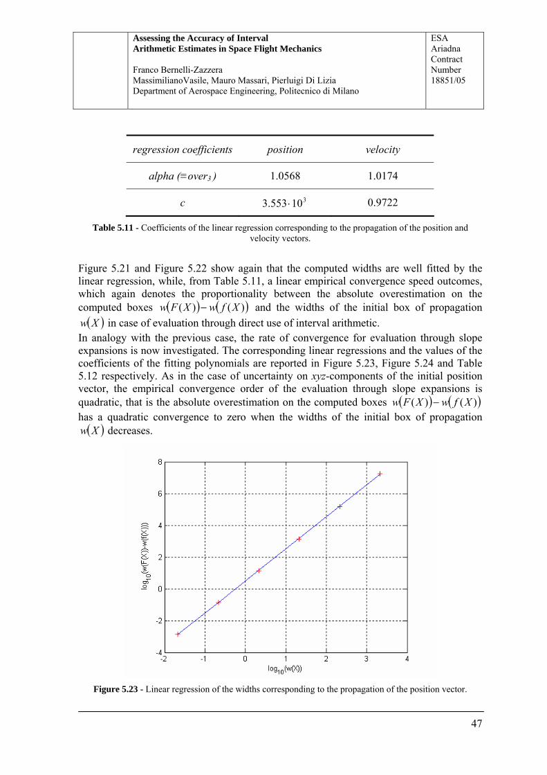
regression coefficients position velocity
alpha (≡over3 ) 1.0568 1.0174
c 3.553 310⋅ 0.9722
Table 5.11 - Coefficients of the linear regression corresponding to the propagation of the position and velocity vectors.
Figure 5.21 and Figure 5.22 show again that the computed widths are well fitted by the linear regression, while, from Table 5.11, a linear empirical convergence speed outcomes, which again denotes the proportionality between the absolute overestimation on the computed boxes ( ) ( ))()( XfwXFw − and the widths of the initial box of propagation ( )Xw in case of evaluation through direct use of interval arithmetic.
In analogy with the previous case, the rate of convergence for evaluation through slope expansions is now investigated. The corresponding linear regressions and the values of the coefficients of the fitting polynomials are reported in Figure 5.23, Figure 5.24 and Table 5.12 respectively. As in the case of uncertainty on xyz-components of the initial position vector, the empirical convergence order of the evaluation through slope expansions is quadratic, that is the absolute overestimation on the computed boxes ( ) ( ))()( XfwXFw − has a quadratic convergence to zero when the widths of the initial box of propagation ( )Xw decreases.
Figure 5.23 - Linear regression of the widths corresponding to the propagation of the position vector.

Assessing the Accuracy of Interval Arithmetic Estimates in Space Flight Mechanics Franco Bernelli-Zazzera MassimilianoVasile, Mauro Massari, Pierluigi Di Lizia Department of Aerospace Engineering, Politecnico di Milano
ESA Ariadna Contract Number 18851/05
48
Figure 5.24 - Linear regression of the widths corresponding to the propagation of the velocity vector.
regression coefficients position velocity
alpha (≡over3 ) 2.0146 2.0024
c 3.1440 5.2556e-004
Table 5.12 - Coefficients of the linear regression corresponding to the propagation of the position and velocity vectors.
5.1.9 Hyperbolic orbits
With the intent of studying the performances of interval analysis in gravity assist manoeuvres, the analytic propagation of the hyperbolic motion in a two-body dynamical model is here investigated. As in the case of the elliptic orbits, the initial position and velocity vectors uniquely identify the motion of a body. Hence, they can be effectively used as orbital parameters to describe the solution of an initial value problem.

Assessing the Accuracy of Interval Arithmetic Estimates in Space Flight Mechanics Franco Bernelli-Zazzera MassimilianoVasile, Mauro Massari, Pierluigi Di Lizia Department of Aerospace Engineering, Politecnico di Milano
ESA Ariadna Contract Number 18851/05
49
By following a procedure similar to the case of paragraph 5.1.1, the Lagrange coefficients of the transition matrix can be derived, which turn out to assume the following form [14]:
)]cosh(1[1 )sinh(
)sinh( )]cosh(1[ )]cosh(1[1
000
0000
00
HHragHH
rra
f
HHarHHa
gHHraf
−−−=−−
−=
−−
+−−=−−−=
&& μ
μμσ
(59)
where a is the semimajor axis of the hyperbola, 0σ and r can be evaluated as:
μσ 00
0vr rr⋅
= (60)
)sinh()cosh()( 0000 HHaHHarar −−+−++−= σ (61) and the term )( 0HH − represents the change in hyperbolic anomaly, which can be related to the true anomaly, f, with the following equation:
H
eef
21tanh
11
21tan
−+
= (62)
Using (59), the initial state vector can be propagated by multiplication with following state transition matrix:
⎥⎦
⎤⎢⎣
⎡=Φ
gfgf&& (63)
where the terms ggff && ,,, here represent 3x3 diagonal matrixes of the corresponding
ggff && ,,, functions defined in (60). The propagation of the initial state vector through the state transition matrix can be seen again as the application of a field 66: RRF →
r defined as:
xxF rrr⋅Φ=)( (64)
to the initial state vector 0xr .

Assessing the Accuracy of Interval Arithmetic Estimates in Space Flight Mechanics Franco Bernelli-Zazzera MassimilianoVasile, Mauro Massari, Pierluigi Di Lizia Department of Aerospace Engineering, Politecnico di Milano
ESA Ariadna Contract Number 18851/05
50
5.1.9.1 The reference orbit
The reference orbit for the propagation in the hyperbolic case has been chosen as an Earth-centred orbit corresponding again to an initial position vector:
{ }0000 rr =r , kmr 65780 = (65)
and an initial velocity vector:
⎭⎬⎫
⎩⎨⎧
+⋅= 0)1(00
0 er
v μr (66)
in an inertial reference frame. The eccentricity has been set to the nominal value 2.1=e . Hence, the orbit results from the propagation of an initial state vector corresponding to the pericenter of a hyperbolic orbit with asymptotic velocity (see Figure 5.25):
skmv / 3.481=∞ (67)
The propagation of uncertainties on initial conditions will be considered in the following paragraphs: a typical relative value of 1% on the corresponding nominal quantities is imposed (see Figure 5.26) and the accuracy of interval arithmetic in enclosing the final solution set is assessed in a way similar to the elliptic case.
Figure 5.25 – Reference orbit for the propagation of hyperbolic motion.
Assessing the Accuracy of Interval Arithmetic Estimates in Space Flight Mechanics Franco Bernelli-Zazzera MassimilianoVasile, Mauro Massari, Pierluigi Di Lizia Department of Aerospace Engineering, Politecnico di Milano
ESA Ariadna Contract Number 18851/05
51
Figure 5.26 – Relative uncertainty of 1% on the y-component of the initial velocity vector; punctual
propagation and inclusion through interval arithmetic.
5.1.9.2 Uncertainty on the xyz-components of the initial position vector
First of all, the case of uncertainty on the xyz-components of the initial position vector is studied, by imposing a relative uncertainty of 1% of the nominal value of the initial velocity vector, resulting in the following three-dimensional box:
[ ]( ) [ ] [ ]{ }0.01 ,01.00.01 ,01.00.01 ,01.0100 −−−+⋅= rrr (68)
In order to avoid the further introduction of numerical errors in the computation deriving from the floating point representation of numbers, the estimation of the overestimation indexes is now performed corresponding to a change in hyperbolic anomaly equal to:
40 =− HH (69)
which nearly corresponds to a distance equal to the radius of the Earth’s sphere of influence. A uniform distribution of 100 punctual vectors on each of the six faces of the initial three-dimensional hypercube is considered and propagated to estimate the range of

Assessing the Accuracy of Interval Arithmetic Estimates in Space Flight Mechanics Franco Bernelli-Zazzera MassimilianoVasile, Mauro Massari, Pierluigi Di Lizia Department of Aerospace Engineering, Politecnico di Milano
ESA Ariadna Contract Number 18851/05
52
the final position and velocity set. The result of such propagation is reported in Figure 5.27 (dots), together with the interval inclusion through interval analysis (box).
Figure 5.27 - Comparison between the final solution set obtained by punctual propagation (dots) and the
corresponding interval inclusion (box) ( 40 =− HH and 2.1=e ).
The evaluation of the overestimation indexes 1over and 2over corresponding to set of the final position vectors ( )(1 rover and )(2 rover ) and velocity vectors ( )(1 vover and
)(2 vover ) is now accomplished in analogy with the elliptical case. Results are reported in Table 5.13, while Figure 5.28 and Figure 5.29 illustrate the convex polytopes enclosing the set of the final position and velocity vectors, which are used for the evaluation of the index
2over . Table 5.13 shows that the situation is quite different from the elliptic case: due to the different form of the Lagrange coefficients, the consequences of the dependency problem, which are mainly related to the overestimation index 1over , are now more evident on the enclosure of the set of the final position vectors than in the case of the velocity vectors; however, due to the shape of the final distribution, the wrapping effect in the inertial reference frame mainly affect the inclusion of the final velocity vectors, resulting in a value of )(2 vover which is twice the corresponding )(2 rover .

Assessing the Accuracy of Interval Arithmetic Estimates in Space Flight Mechanics Franco Bernelli-Zazzera MassimilianoVasile, Mauro Massari, Pierluigi Di Lizia Department of Aerospace Engineering, Politecnico di Milano
ESA Ariadna Contract Number 18851/05
53
Overestimation index e = 1.2
over1(r) 0.9063
over1(v) 0.1593
over2(r) 7.2849
over2(v) 13.0982
Table 5.13 - Overestimation indexes over1 and over2 for the position and velocity vectors.
Figure 5.28 - Comparison between the minimum convex polytope enclosing the final solution set of position vectors obtained by punctual propagation and the corresponding interval inclusion (box) ( 40 =− HH and
2.1=e ).

Assessing the Accuracy of Interval Arithmetic Estimates in Space Flight Mechanics Franco Bernelli-Zazzera MassimilianoVasile, Mauro Massari, Pierluigi Di Lizia Department of Aerospace Engineering, Politecnico di Milano
ESA Ariadna Contract Number 18851/05
54
Figure 5.29 - Comparison between the minimum convex polytope enclosing the final solution set of velocity vectors obtained by punctual propagation and the corresponding interval inclusion (box) ( 40 =− HH and
2.1=e ).
5.1.9.3 Overestimation trend along the orbit
The trend of the overestimation indexes 1over and 2over along the orbit is now assessed through the evaluation of their values corresponding to five hyperbolic anomaly changes:
5,...,10 =− HH (70)
Table 5.14 reports the corresponding results. It is worth observing that the overestimation index over1(r) tend to increase while moving away from Earth, thus highlighting an evident loss of accuracy in identifying the set of asymptotic position vectors. This is not the case for the set of asymptotic velocity vectors, due to the less sensitivity of the final set on uncertainties on initial position vector. Such a feature can be effectively highlighted through the computation of the Jacobian matrix of the field (64) with respect to the initial position vector. After a normalization of the field through the definition of a reference length, d, equal to the Earth’s mean radius (6378 km) and the normalized position and velocity vectors, *rr and *vr , as:

Assessing the Accuracy of Interval Arithmetic Estimates in Space Flight Mechanics Franco Bernelli-Zazzera MassimilianoVasile, Mauro Massari, Pierluigi Di Lizia Department of Aerospace Engineering, Politecnico di Milano
ESA Ariadna Contract Number 18851/05
55
drrr
r=* (71)
d
vvμ
rr
=* (72)
the Euclidean norm of the rows of the Jacobian matrix, corresponding to the norm of the gradients with respect to the initial position vector, evaluated at 4)( 0 =− HH , turns out to be:
410
0.00040.00570.003660.41412.08468.2512
)2,(0
−⋅
⎪⎪⎪⎪
⎭
⎪⎪⎪⎪
⎬
⎫
⎪⎪⎪⎪
⎩
⎪⎪⎪⎪
⎨
⎧
=rJnorm r (73)
which confirm the previous observation.
H over1(r) over1(v) over2(r) over2(v)
0.1 0.2866 1.2474 1.8853 9.4010
0.5 0.4167 0.1180 7.4841 4.7690
1 0.5990 0.0853 8.7649 6.5555
2 0.8049 0.1444 7.8867 10.7936
3 0.8788 0.1559 7.4501 12.4607
4 0.9062 0.1594 7.2849 13.0982
5 0.9164 0.1606 7.2239 13.3363
Table 5.14 – Overestimation indexes trend along the orbit.

Assessing the Accuracy of Interval Arithmetic Estimates in Space Flight Mechanics Franco Bernelli-Zazzera MassimilianoVasile, Mauro Massari, Pierluigi Di Lizia Department of Aerospace Engineering, Politecnico di Milano
ESA Ariadna Contract Number 18851/05
56
5.1.9.4 Overestimation index over3
The estimation of the overestimation index 3over is now addressed for evaluating the convergence speed of the adopted inclusion function. The index is again evaluated separately for the propagation of position and velocity vectors by performing the linear regression over five sample initial boxes obtained by imposing a relative uncertainty with respect to the nominal value of the initial position vector equal to n−10 , 5,...,1=n . The final hypercube is computed corresponding to a hyperbolic anomaly change of
40 =− HH . Figure 5.30 and Figure 5.31 report the results of the linear regressions corresponding to the propagation of the position and velocity vectors respectively, while Table 5.15 reports the values of the coefficients of the corresponding polynomials.
Figure 5.30 – Linear regression of the widths corresponding to the propagation of the position vector.

Assessing the Accuracy of Interval Arithmetic Estimates in Space Flight Mechanics Franco Bernelli-Zazzera MassimilianoVasile, Mauro Massari, Pierluigi Di Lizia Department of Aerospace Engineering, Politecnico di Milano
ESA Ariadna Contract Number 18851/05
57
Figure 5.31 - Linear regression of the widths corresponding to the propagation of the velocity vector.
regression coefficients position velocity
alpha (≡over3 ) 1.0068 1.0087
c 427.9600 2.0079 1110−⋅
Table 5.15 – Coefficients of the linear regression corresponding to the propagation of the position and velocity vectors.
The computed widths are well fitted by the linear regression and the empirical convergence speed, which coincides with the overestimation index 3over , is nearly equal to 1 in both the cases of propagation of position and velocity vectors, showing again a linear behaviour of the inclusion function, that is the absolute overestimation on the computed boxes ( ) ( ))()( XfwXFw − tends to be proportional to the widths of the initial box of propagation ( )Xw .
The case of the use of slope expansions is now investigated. The corresponding linear regressions and the values of the coefficients of the fitting polynomials are reported in Figure 5.32, Figure 5.33 and Table 5.16 respectively. The empirical convergence order of

Assessing the Accuracy of Interval Arithmetic Estimates in Space Flight Mechanics Franco Bernelli-Zazzera MassimilianoVasile, Mauro Massari, Pierluigi Di Lizia Department of Aerospace Engineering, Politecnico di Milano
ESA Ariadna Contract Number 18851/05
58
the evaluation through slope expansions confirms to be quadratic: the absolute overestimation on the computed boxes ( ) ( ))()( XfwXFw − has a quadratic convergence to zero when the widths of the initial box of propagation ( )Xw decreases.
Figure 5.32 - Linear regression of the widths corresponding to the propagation of the position vector.
Figure 5.33 - Linear regression of the widths corresponding to the propagation of the velocity vector.

Assessing the Accuracy of Interval Arithmetic Estimates in Space Flight Mechanics Franco Bernelli-Zazzera MassimilianoVasile, Mauro Massari, Pierluigi Di Lizia Department of Aerospace Engineering, Politecnico di Milano
ESA Ariadna Contract Number 18851/05
59
regression coefficients position velocity
alpha (≡over3 ) 2.0052 1.9350
c 8.8213 410−⋅ 4.7799 1610−⋅
Table 5.16 - Coefficients of the linear regression corresponding to the propagation of the position and velocity vectors.
5.2 Validated Propagation of elliptic orbits
The validated propagation of motion in a two-body dynamical framework with initial conditions corresponding to elliptic orbits is now investigated. Heliocentric orbits have been studied in a units system which measures distances in astronomical units (AU) and time in a system where 2 π time units (TU) equal one earth year (see Berz, Hoefkens and Makino [21]). As the orbit eccentricity constitutes an important parameter affecting the dynamic of the problem, the initial conditions have been set to obtain orbits with eccentricity nominal values of 0.0, 0.5 and 0.9, starting from the pericenter:
{ }
⎭⎬⎫
⎩⎨⎧
+=
=
010
00
00
00
er
v
rr
μr
r
(74)
where 0r has been set to AU 10 =r . Integrations have been performed for a maximum of 10 orbits. The uncertainties on the initial conditions (74) have been obtained as interval enclosures by simply adding:
[ ][ ] AU/TU 105.0
AU 105.0
00
00n
n
vv
rr−
−
⋅±=
⋅±=rr
rr
(75)
to all components of 0r
r and 0vr , with n a positive integer. In the following, the validated integration of elliptic orbits is first addressed in the case of absence of uncertainty and the performances of each validated integration tool are studied and compared with those achievable by means of symplectic integrators.

Assessing the Accuracy of Interval Arithmetic Estimates in Space Flight Mechanics Franco Bernelli-Zazzera MassimilianoVasile, Mauro Massari, Pierluigi Di Lizia Department of Aerospace Engineering, Politecnico di Milano
ESA Ariadna Contract Number 18851/05
60
After that, the introduction of uncertainty on the initial position and velocity vector is considered and results are compared again.
5.2.1 Point initial conditions
The case of punctual initial conditions is now studied: initial conditions have been set using equation (94) without uncertainty. As an illustrative example, Figure 5.34 reports the orbit and its projection into the phase space obtained by means of an Interval Taylor Series method using VNODE in the case of
5.0=e and compares it with the analytic propagation. As can be seen, results of VNODE can be unlikely recognized: this is due to the fact that VNODE produced in this case a validate results which accurately enclose the analytic solutions in intervals of very little widths, as will be illustrated next. However, Figure 5.34 also reports the enclosure of the energy over the propagated orbits: intervals become larger and larger during the integration process in fact, even if the ITS method could integrate the overall 10 orbits.
Figure 5.34 - Orbit and its projection into the phase space obtained by means of an Interval Taylor Series
method using VNODE (blue) and analytic propagation (red) in the case of 5.0=e . Top-right figure: energy enclosure.

Assessing the Accuracy of Interval Arithmetic Estimates in Space Flight Mechanics Franco Bernelli-Zazzera MassimilianoVasile, Mauro Massari, Pierluigi Di Lizia Department of Aerospace Engineering, Politecnico di Milano
ESA Ariadna Contract Number 18851/05
61
This is not the case when high eccentricity values are investigated: Figure 5.35 reports the same results corresponding to an eccentricity value of 9.0=e . It can be seen that the growth of the interval widths is now remarkable and the integration process produces useless results after 4.5 orbits. Table 5.17 reports the maximum number of orbits propagated by the tested validated integration tools corresponding to the different eccentricity value. In all cases the order of the integrators has been set to 18, with a maximum local error of 1110− and a variable stepsize control. First of all, it should be noted that all the test tools could not integrate punctual initial conditions corresponding to a circular orbit. This problem has been solved in AWA by setting an interval uncertainty on the initial conditions of 1610− ; however, the same approach could be used with VNODE, which required an uncertainty of 810− at least, which can not be considered as punctual. This problem disappears when integrating orbits with an eccentricity greater than 0.05. Secondly, note that no one of the tested tools could reach the maximum integration time of 10 orbits in the case of 9.0=e , which constitute a hard benchmark problem for numerical integration algorithms in general.
Figure 5.35 - Orbit and its projection into the phase space obtained by means of an Interval Taylor Series
method using VNODE (blue) and analytic propagation (red) in the case of 9.0=e . Top-right figure: energy enclosure.

Assessing the Accuracy of Interval Arithmetic Estimates in Space Flight Mechanics Franco Bernelli-Zazzera MassimilianoVasile, Mauro Massari, Pierluigi Di Lizia Department of Aerospace Engineering, Politecnico di Milano
ESA Ariadna Contract Number 18851/05
62
Integrator 0.0=e 5.0=e 9.0=e
AWA 10 5.814 1.972
ITS (VNODE) - 10 4.878
IHO (VNODE) - 10 4.159
Table 5.17 – Number of orbits propagated by the tested validated integration tools corresponding to the different eccentricity value.
Let now consider the trend of the interval widths over the integration time interval. Figure 5.36, Figure 5.37 and Figure 5.38 report the interval widths of to the position and velocity vectors for each validated integrator corresponding to an eccentricity value 5.0=e . It is important to note that, after a first spot of sub-exponential behaviour, the growth of the intervals widths is nearly exponential with respect to the integration time in both position and velocity, although little oscillations occur whose period are related that of the orbit. Moreover, such oscillations can be easily recognized when the trend of the stepsize is analysed. Figure 5.39 plots the stepsize with respect to the integration time (reported as number of orbits) corresponding to each validated integration tool. As can be easily noted, the stepsize has an oscillating trend in all cases with a period equal to the period of the orbit: the minimum value of the stepsize corresponds to the pericenter of the orbit, where the high derivatives of the state vector occur, while the maximum is reached to the apocenter. Note that, although AWA and ITS implements the same integration scheme, the former turns out to allows higher integration steps, which, however, correspond to wider inclusion intervals (compare Figure 5.36 and Figure 5.37): such differences in the step control scheme may be investigated as the reason of the premature integration break of AWA, together with the choice of the initial stepsize, which is automatically evaluated by VNODE, while externally imposed in AWA (here set to 0.1, which seemed a good choice as the result produced by VNODE confirms). Moreover, it is worth noting that, the growth of the interval widths being nearly equal, IHO scheme allows greater stepsizes than ITS scheme, as already pointed out by Nedialkov [9].

Assessing the Accuracy of Interval Arithmetic Estimates in Space Flight Mechanics Franco Bernelli-Zazzera MassimilianoVasile, Mauro Massari, Pierluigi Di Lizia Department of Aerospace Engineering, Politecnico di Milano
ESA Ariadna Contract Number 18851/05
63
Figure 5.36 – Widths of the position vector (left) and the velocity vector (right) for the case of AWA ( 5.0=e )
Figure 5.37 - Widths of the position vector (left) and the velocity vector (right) for the case of ITS ( 5.0=e )
Figure 5.38 - Widths of the position vector (left) and the velocity vector (right) for the case of IHO ( 5.0=e )

Assessing the Accuracy of Interval Arithmetic Estimates in Space Flight Mechanics Franco Bernelli-Zazzera MassimilianoVasile, Mauro Massari, Pierluigi Di Lizia Department of Aerospace Engineering, Politecnico di Milano
ESA Ariadna Contract Number 18851/05
64
Figure 5.39 – Comparison between the stepsize trends corresponding to each validated integration tool
( 5.0=e ).
5.2.1.1 Results comparison varying the eccentricity value
Let now compare the results obtained with each validated integration tool at various eccentricity level. To this aim, let define a medium intervals width of the position vector,
)(rwmr as:
)()()()( 32
22
12 rwrwrwrwm ++=
r (76)
which represents in fact the width of the diagonal of the interval box on the position vector ][rr and which can be used here to gain insight on the medium behaviour of the interval
growth. Figure 5.40, Figure 5.41 and Figure 5.42 report the trend of )(rwm
r corresponding to different values of eccentricity for each tested tool. Note that in case of VNODE, an eccentricity value of 0.05 has been considered as representative of the behaviour of the method at low eccentricity values. An important observation can be stated by these figures: the rate of the exponential growth increases with the eccentricity of the orbit, which confirms to be an important parameter affecting the stability of the validated integration tools. This is much more evident when passing from medium eccentricity values to high

Assessing the Accuracy of Interval Arithmetic Estimates in Space Flight Mechanics Franco Bernelli-Zazzera MassimilianoVasile, Mauro Massari, Pierluigi Di Lizia Department of Aerospace Engineering, Politecnico di Milano
ESA Ariadna Contract Number 18851/05
65
ones. Moreover it is worth noting how IHO method allows a better control of the interval growth as the eccentricity of the orbit increases, especially corresponding to the first orbit, where the sub-exponential behaviour persists.
Figure 5.40 - Trend of )(rwm
r corresponding to different eccentricity values for AWA.
Figure 5.41 - Trend of )(rwm
r corresponding to different eccentricity values for ITS.

Assessing the Accuracy of Interval Arithmetic Estimates in Space Flight Mechanics Franco Bernelli-Zazzera MassimilianoVasile, Mauro Massari, Pierluigi Di Lizia Department of Aerospace Engineering, Politecnico di Milano
ESA Ariadna Contract Number 18851/05
66
Figure 5.42 - Trend of )(rwm
r corresponding to different eccentricity values for IHO.
Finally, Figure 5.43, Figure 5.44 and Figure 5.45 compare the stepsize trends of each tested tool corresponding to the different eccentricity values. Corresponding to very low eccentricity values, all the tested tools present strange oscillation of the stepsize during the integration process: this should be investigated as a possible explanation of the strange behaviour of all tested tools corresponding to circular orbits. The periodicity of the stepsize trend with respect to the number of the propagated orbits is then evident for 0.5 eccentric orbits. Moreover, it is interesting to observe as AWA seems to reach a maximum stepsize value of 1 TU corresponding to the apogee of the elliptic orbit. Such limitation should not be considered as the reason of the worse performances of AWA: indeed, in the case of eccentricity 5.0=e , the limit of 1 TU is not reached, even if AWA could not integrate 10 orbits as ITS and IHO can do.

Assessing the Accuracy of Interval Arithmetic Estimates in Space Flight Mechanics Franco Bernelli-Zazzera MassimilianoVasile, Mauro Massari, Pierluigi Di Lizia Department of Aerospace Engineering, Politecnico di Milano
ESA Ariadna Contract Number 18851/05
67
Figure 5.43 - AWA stepsize trend at different eccentricity values.
Figure 5.44 - ITS stepsize trend at different eccentricity values.

Assessing the Accuracy of Interval Arithmetic Estimates in Space Flight Mechanics Franco Bernelli-Zazzera MassimilianoVasile, Mauro Massari, Pierluigi Di Lizia Department of Aerospace Engineering, Politecnico di Milano
ESA Ariadna Contract Number 18851/05
68
Figure 5.45 - IHO stepsize trend at different eccentricity values.
5.2.1.2 Results comparison at fixed eccentricity values
Consider now the comparison of the performances of each integration tool at fixed eccentricity values. The definition of the medium intervals width of the position vector,
)(rwmr , given in equation (96), is deemed again as representative of the medium behaviour.
Figure 5.46, Figure 5.47 and Figure 5.48 report the trend of )(rwmr corresponding to the
different tested tools by fixing the eccentricity value. Note that, due to the lack of information on VNODE performances corresponding to circular orbits, the comparison reported in Figure 5.46 is strictly valid between ITS and IHO methods only. First of all it is important to point out that the, after the first sub-exponential phase, the rate of the exponential growth is nearly equal for all the tested tools: such result indicates that the rate of the exponential growth depends only on the eccentricity of the orbit and does not display relevant differences between the different tools, especially comparing ITS and IHO methods. Secondly, the results indicate that the algorithms implemented in VNODE seem to be preferable to AWA both in the ITS and IHO method. Moreover, although both IHO and ITS methods could reach the final time of integration of 10 orbits at 05.0=e and 5.0=e , ITS results present lower values of the medium intervals width of the position vector, so indicating less overestimation than the IHO method. In conclusion, it can be stated that ITS

Assessing the Accuracy of Interval Arithmetic Estimates in Space Flight Mechanics Franco Bernelli-Zazzera MassimilianoVasile, Mauro Massari, Pierluigi Di Lizia Department of Aerospace Engineering, Politecnico di Milano
ESA Ariadna Contract Number 18851/05
69
method outperforms both IHO and AWA methods in the integration of elliptic orbits when studying punctual initial conditions.
Figure 5.46 – Comparison of the trends of )(rwm
r corresponding to the different tested tools ( 0=e for
AWA, 05.0=e for ITS and IHO).
Figure 5.47 - Comparison of the trends of )(rwm
r corresponding to the different tested tools ( 5.0=e )

Assessing the Accuracy of Interval Arithmetic Estimates in Space Flight Mechanics Franco Bernelli-Zazzera MassimilianoVasile, Mauro Massari, Pierluigi Di Lizia Department of Aerospace Engineering, Politecnico di Milano
ESA Ariadna Contract Number 18851/05
70
Figure 5.48 - Comparison of the trends of )(rwm
r corresponding to the different tested tools ( 5.0=e ).
5.2.1.3 The use of symplectic integrators
For the sake of a complete analysis of the advantages of validated integrators with respect to classical numerical integration scheme, the purpose of this section is studying the performances of classical numerical integration schemes and comparing them with results achieved in the previous paragraphs. The integration of motion in the case of elliptic orbits has been accomplished by means of five classical integration algorithms: (1) A 4th order explicit Runge-Kutta scheme with variable stepsize control, relative
tolerance 310− and absolute tolerance 610− (RK expl 4, varstep); (2) A 4th order explicit Runge-Kutta scheme with fixed stepsize (RK expl 4, fixstep); (3) A 4th order implicit Runge-Kutta scheme with fixed stepsize (RK impl 4) (4) A 8th order implicit Runge-Kutta scheme with fixed stepsize (RK impl 8); (5) A 12th order implicit Runge-Kutta scheme with fixed stepsize (RK impl 12). All the implicit Runge-Kutta schemes have been demonstrated to be symplectic [22] and then particularly effective for the integration of Hamiltonian systems dynamics. A stepsize of 0.01 TU has been set in all the fixed point numerical schemes, as this resulted to be the minimum value required by the validated integration schemes (see Figure 5.39). All the classical numerical integration algorithms could reach the final time of integration of 10 orbits. However, errors in the determination of the state vector have been obviously

Assessing the Accuracy of Interval Arithmetic Estimates in Space Flight Mechanics Franco Bernelli-Zazzera MassimilianoVasile, Mauro Massari, Pierluigi Di Lizia Department of Aerospace Engineering, Politecnico di Milano
ESA Ariadna Contract Number 18851/05
71
quite different. As an example, let us check the results of the 4th order explicit Runge-Kutta scheme with variable stepsize control corresponding to the most challenging 0.9 eccentric orbit. Figure 5.49 reports the orbit and the projection of the state vector into the phase space, together with the trend of the energy value. As can be readily recognized the error on the identification of the state vector increases with time and is maximum at the apocenter of the orbit, while low performances occur in the preservation of the energy value. The situation greatly change when the symplectic 12th order implicit Runge-Kutta method is used, whose results are reported in Figure 5.50: here, the numerical solution can not be distinguished from the analytical one in figure and the energy is accurately preserved.
Figure 5.49 – Integration of an elliptic orbit with 9.0=e using a 4th order explicit Runge-Kutta scheme
with variable stepsize control (blue). Comparison with the analytic solution (red).

Assessing the Accuracy of Interval Arithmetic Estimates in Space Flight Mechanics Franco Bernelli-Zazzera MassimilianoVasile, Mauro Massari, Pierluigi Di Lizia Department of Aerospace Engineering, Politecnico di Milano
ESA Ariadna Contract Number 18851/05
72
Figure 5.50 – Integration of an elliptic orbit with 9.0=e using a symplectic 12th order implicit Runge-
Kutta scheme with fixed stepsize (blue). Comparison with the analytic solution (red).
Let now consider the numerical integration error. Figure 5.51, Figure 5.52 and Figure 5.53 report the trend of the integration error of classical integration algorithms (defined as the maximum norm of the difference vector between the numerical and the exact state vectors). As can be noted, symplectic integrators outperforms the other classical numerical schemes, even if low order is used, especially at high eccentricity values; moreover, the precision obtained by high order symplectic schemes is quite impressive: they could integrate all elliptic orbits very accurately, with an error oscillating between 1510− (near the floating-point relative accuracy, 522− ).

Assessing the Accuracy of Interval Arithmetic Estimates in Space Flight Mechanics Franco Bernelli-Zazzera MassimilianoVasile, Mauro Massari, Pierluigi Di Lizia Department of Aerospace Engineering, Politecnico di Milano
ESA Ariadna Contract Number 18851/05
73
Figure 5.51 – Comparison between the error trend of the classical numerical integrators and the maximum
interval width of the ITS validated integration method. Orbit eccentricity 05.0=e .
Figure 5.52 - Comparison between the error trend of the classical numerical integrators and the maximum
interval width of the ITS validated integration method. Orbit eccentricity 5.0=e .

Assessing the Accuracy of Interval Arithmetic Estimates in Space Flight Mechanics Franco Bernelli-Zazzera MassimilianoVasile, Mauro Massari, Pierluigi Di Lizia Department of Aerospace Engineering, Politecnico di Milano
ESA Ariadna Contract Number 18851/05
74
Figure 5.53 - Comparison between the error trend of the classical numerical integrators and the maximum
interval width of the ITS validated integration method. Orbit eccentricity 9.0=e .
Figure 5.51, Figure 5.52 and Figure 5.53 also reports the performances of the ITS validated integration method for comparison purposes: in particular, the maximum of the interval widths of the components of the interval state vector is illustrated, that is:
])([max])([
,...,1max inixwxw
== (77)
where n is the number of the dimension of the state vector:
⎭⎬⎫
⎩⎨⎧
=][][
][vr
x
Even if the results of the validated integration are not comparable with those of classical integration schemes, because of different concepts motivate the two integration techniques and then different approaches are used to define the solution of the integration process, such comparison can roughly illustrate the precision and correctness of solutions of the classical integration schemes. As can be noted from the previous figures, the error of the high order symplectic integration algorithms are always lower than the maximum width of

Assessing the Accuracy of Interval Arithmetic Estimates in Space Flight Mechanics Franco Bernelli-Zazzera MassimilianoVasile, Mauro Massari, Pierluigi Di Lizia Department of Aerospace Engineering, Politecnico di Milano
ESA Ariadna Contract Number 18851/05
75
the interval solution; in fact, after a careful analysis, the solution of such integration algorithms turned out to be inside the boxes defining the interval solution. This is not the case for lower order classical integration schemes, which start to belong to the interval solution only after some 2-3 orbits, when the growth of the interval widths of the validated solution allowed such inclusion. It is worth highlighting that such conclusions do not enable stating that high order symplectic integration schemes are preferable to the validated integration: indeed the classical integration schemes aim at reaching a numerical solution of the ordinary differential equation with a certain accuracy, so that at the end of the integration process one gets a punctual solution which approximates the exact solution with a certain accuracy, which can suffice in many practical applications; the validated integration algorithms can produce interval solutions which certainly include the exact solution of the differential equation, so enabling validated analysis for further computations, which allows avoiding errors related to bad numerical approximations. As a consequence, the choice of the integration technique is strictly related to the problem at hand. However it is worth noting that: • the previous analysis has been conducted on the integration of an Hamiltonian system,
where symplectic integrators produce their best performances; • the validated integration techniques can also handle interval initial conditions and
interval parameters defining the dynamics of the problem, which allows propagating also uncertainties during the integration process (even if the interval growth seems to lead to useless results when studying long term propagation).
5.2.2 Uncertain initial conditions
Apart from the important advantages of validated integrators of producing validated solutions of ordinary differential equations, they offer the interesting possibility of handling uncertainty on the initial conditions and on the dynamical model parameters by including them in suitable interval numbers and interval vectors. The performances of the validated tools at integrating elliptic orbits with interval initial conditions are now investigated. Initial conditions of the form (94) are considered and uncertainties are introduced separately on the position and velocity vectors using the procedure described in equation (95), which is here reported again:
[ ][ ] AU/TU 10
AU 10
00
00n
n
vv
rr−
−
±=
±=rr
rr
with 7,...,3=n . The maximum uncertainty is fixed 3=n , where all tested tools could not integrate more than one orbit. The following subsections analyse the performances of the tested tools corresponding to uncertainties on the initial position and velocity vectors respectively.

Assessing the Accuracy of Interval Arithmetic Estimates in Space Flight Mechanics Franco Bernelli-Zazzera MassimilianoVasile, Mauro Massari, Pierluigi Di Lizia Department of Aerospace Engineering, Politecnico di Milano
ESA Ariadna Contract Number 18851/05
76
5.2.2.1 Uncertainty on the initial position vector
Table 5.18, Table 5.19 and Table 5.20 report the number of orbits propagated by each validated tool corresponding to various eccentricity values for different levels of uncertainty on the initial position vector. First of all note that all validated integration tools could not integrate the maximum of 10 orbits in all cases, even when circular orbits are considered: even introducing an uncertainty of 710− AU (which is typical for celestial small-bodies position measurements), performances decrease significantly. A representative example is that of the ITS method: when propagating an elliptic orbit with eccentricity 0.5 and punctual initial conditions, this method can integrate 10 orbits (see Table 5.17); but the introduction of an uncertainty of 710− AU on the initial position vector leads to a number of propagated orbits equal to 4.8820, that is less than half. The situation drastically worsens with high uncertainty values: indeed, as can be readily recognized, the number of propagated orbits decreases significantly with increasing eccentricity (as also obtained in case of punctual initial conditions) and with increasing uncertainty levels. The previous observations can be highlighted by reporting the growth of the medium intervals width defined in equation (96). Figures from Figure 5.54 to Figure 5.62 report the trend of )(rwm as a function of the propagated orbits to compare the performances of each tested tool at various uncertainty levels by fixing the eccentricity value. The rate of the intervals growth significantly increases with the uncertainty on the initial position vector, by evidently anticipating the beginning of the super-exponential growth, which typically immediately precedes the integration process break in all tested tools.
uncertainty eccentricity
position velocity e = 0.0 e = 0.5 e = 0.9 710− 0 8.9576 4.1541 1.8577 610− 0 4.9885 2.9018 1.0345 510− 0 2.7146 1.8392 0.9979 410− 0 1.2532 1.0861 0.9745 310− 0 0.7360 0.8140 0.3162
Table 5.18 - Number of propagated orbits corresponding to different position uncertainty levels.
AWA (18th order, Absolute Tolerance 10-11).

Assessing the Accuracy of Interval Arithmetic Estimates in Space Flight Mechanics Franco Bernelli-Zazzera MassimilianoVasile, Mauro Massari, Pierluigi Di Lizia Department of Aerospace Engineering, Politecnico di Milano
ESA Ariadna Contract Number 18851/05
77
uncertainty eccentricity
position velocity e = 0.0 e = 0.5 e = 0.9 710− 0 9.2136 4.8820 1.9662 610− 0 5.2985 2.9621 1.0395 510− 0 2.9159 1.9502 0.9975 410− 0 1.4998 1.0502 0.9826 310− 0 0.7734 0.9176 0.8297
Table 5.19 - Number of propagated orbits corresponding to different position uncertainty levels.
ITS method (18th order, Absolute Tolerance 10-11).
uncertainty eccentricity
position velocity e = 0.0 e = 0.5 e = 0.9 710− 0 9.2088 4.9174 1.9692 610− 0 5.3437 2.9658 1.0437 510− 0 2.9406 1.9485 0.9972 410− 0 1.5109 1.0481 0.9808 310− 0 0.7700 0.9089 0.8108
Table 5.20 - Number of propagated orbits corresponding to different position and velocity uncertainty levels.
IHO method (18th order, Absolute Tolerance 10-11).

Assessing the Accuracy of Interval Arithmetic Estimates in Space Flight Mechanics Franco Bernelli-Zazzera MassimilianoVasile, Mauro Massari, Pierluigi Di Lizia Department of Aerospace Engineering, Politecnico di Milano
ESA Ariadna Contract Number 18851/05
78
Figure 5.54 - Trend of )(rwm corresponding to different uncertainty levels; AWA, 0.0=e .
Figure 5.55 - Trend of )(rwm corresponding to different uncertainty levels; AWA, 5.0=e .

Assessing the Accuracy of Interval Arithmetic Estimates in Space Flight Mechanics Franco Bernelli-Zazzera MassimilianoVasile, Mauro Massari, Pierluigi Di Lizia Department of Aerospace Engineering, Politecnico di Milano
ESA Ariadna Contract Number 18851/05
79
Figure 5.56 - Trend of )(rwm corresponding to different uncertainty levels; AWA, 9.0=e .
Figure 5.57 - Trend of )(rwm corresponding to different uncertainty levels; ITS, 0.0=e .

Assessing the Accuracy of Interval Arithmetic Estimates in Space Flight Mechanics Franco Bernelli-Zazzera MassimilianoVasile, Mauro Massari, Pierluigi Di Lizia Department of Aerospace Engineering, Politecnico di Milano
ESA Ariadna Contract Number 18851/05
80
Figure 5.58 - Trend of )(rwm corresponding to different uncertainty levels; ITS, 5.0=e .
Figure 5.59 - Trend of )(rwm corresponding to different uncertainty levels; ITS, 9.0=e .

Assessing the Accuracy of Interval Arithmetic Estimates in Space Flight Mechanics Franco Bernelli-Zazzera MassimilianoVasile, Mauro Massari, Pierluigi Di Lizia Department of Aerospace Engineering, Politecnico di Milano
ESA Ariadna Contract Number 18851/05
81
Figure 5.60 - Trend of )(rwm corresponding to different uncertainty levels; IHO, 0.0=e .
Figure 5.61 - Trend of )(rwm corresponding to different uncertainty levels; IHO, 5.0=e .

Assessing the Accuracy of Interval Arithmetic Estimates in Space Flight Mechanics Franco Bernelli-Zazzera MassimilianoVasile, Mauro Massari, Pierluigi Di Lizia Department of Aerospace Engineering, Politecnico di Milano
ESA Ariadna Contract Number 18851/05
82
Figure 5.62 - Trend of )(rwm corresponding to different uncertainty levels; IHO, 9.0=e .
Let now report results of the previous tables in a different form. Table 5.21, Table 5.22 and Table 5.23 reports the number of propagated orbits by fixing the eccentricity value and comparing the performances of each validated tool. Little differences can be recognized between the two validated integrators supplied by VNODE. However, AWA generally performed worse than ITS and IHO methods: this constitutes again an interesting result because ITS method implemented in VNODE is in fact similar to the method implemented in AWA. However, the stepsize control law and the automatic selection of the initial stepsize implemented in VNODE results to improve the tool performances.
uncertainty eccentricity position velocity AWA ITS IHO
710− 0 8.9576 9.2136 9.2088 610− 0 4.9885 5.2985 5.3437 510− 0 2.7146 2.9159 2.9406 410− 0 1.2532 1.4998 1.5109 310− 0 0.7360 0.7734 0.7700
Table 5.21 - Number of orbits propagated by each tool corresponding to different position uncertainty levels ( 0.0=e ).

Assessing the Accuracy of Interval Arithmetic Estimates in Space Flight Mechanics Franco Bernelli-Zazzera MassimilianoVasile, Mauro Massari, Pierluigi Di Lizia Department of Aerospace Engineering, Politecnico di Milano
ESA Ariadna Contract Number 18851/05
83
uncertainty eccentricity
position velocity AWA ITS IHO 710− 0 4.1541 4.8820 4.9174 610− 0 2.9018 2.9621 2.9658 510− 0 1.8392 1.9502 1.9485 410− 0 1.0861 1.0502 1.0481 310− 0 0.8140 0.9176 0.9089
Table 5.22 - Number of orbits propagated by each tool corresponding to different position uncertainty levels ( 5.0=e ).
uncertainty eccentricity
position velocity AWA ITS IHO 710− 0 1.8577 1.9662 1.9692 610− 0 1.0345 1.0395 1.0437 510− 0 0.9979 0.9975 0.9972 410− 0 0.9745 0.9826 0.9808 310− 0 0.3162 0.8297 0.8108
Table 5.23 - Number of orbits propagated by each tool corresponding to different position uncertainty levels ( 9.0=e ).
Such results are confirmed by Figure 5.63, Figure 5.64 and Figure 5.65, where the performances of the tested tools are compared at fixed eccentricity values. The stepsize trend over the time span of integration does not show dependence on the uncertainty level, as indicated in Figure 5.66, Figure 5.67 and Figure 5.68 for the case of nominal circular orbit (the situation does not change corresponding to other eccentricity values): the stepsize history is nearly identical in all cases until the integration break occurs. Moreover, as already mentioned, note the oscillation of the stepsize trend at low eccentricity values.

Assessing the Accuracy of Interval Arithmetic Estimates in Space Flight Mechanics Franco Bernelli-Zazzera MassimilianoVasile, Mauro Massari, Pierluigi Di Lizia Department of Aerospace Engineering, Politecnico di Milano
ESA Ariadna Contract Number 18851/05
84
Figure 5.63 – Comparison of the )(rwm trend corresponding to different uncertainty levels; 0.0=e .
Figure 5.64 - Comparison of the )(rwm trend corresponding to different uncertainty levels; 5.0=e .

Assessing the Accuracy of Interval Arithmetic Estimates in Space Flight Mechanics Franco Bernelli-Zazzera MassimilianoVasile, Mauro Massari, Pierluigi Di Lizia Department of Aerospace Engineering, Politecnico di Milano
ESA Ariadna Contract Number 18851/05
85
Figure 5.65 - Comparison of the )(rwm trend corresponding to different uncertainty levels; 9.0=e .
Figure 5.66 - Stepsize trends over the time of integration at different uncertainty levels, AWA.

Assessing the Accuracy of Interval Arithmetic Estimates in Space Flight Mechanics Franco Bernelli-Zazzera MassimilianoVasile, Mauro Massari, Pierluigi Di Lizia Department of Aerospace Engineering, Politecnico di Milano
ESA Ariadna Contract Number 18851/05
86
Figure 5.67 - Stepsize trends over the time of integration at different uncertainty levels, ITS.
Figure 5.68 - Stepsize trends over the time of integration at different uncertainty levels, IHO.

Assessing the Accuracy of Interval Arithmetic Estimates in Space Flight Mechanics Franco Bernelli-Zazzera MassimilianoVasile, Mauro Massari, Pierluigi Di Lizia Department of Aerospace Engineering, Politecnico di Milano
ESA Ariadna Contract Number 18851/05
87
5.2.2.1.1 Overestimation indexes
The evaluation of the overestimation associated to the validated integration processes is here addressed by analysing the trend of the overestimation indexes 1over and 2over (see Paragraph 5.1.2) during the integration process. In particular, due to the high computational effort required by the estimation of such indexes, five sample points have been chosen as representative of the integrators behaviour, corresponding to the following time of integration:
nTTTTTtover ,
43,
21,
41
+⎭⎬⎫
⎩⎨⎧=
where T is the orbit period and n is a positive integer indicating the number of propagated orbits. First of all, let compare the overestimation indexes history at various eccentricity values by fixing the uncertainty level to 710− AU. Figure 5.85, Figure 5.86 and Figure 5.87 illustrate the results obtained for the overestimation of the sets of both position and velocity vectors for each tested tool. The previous figures show that the overestimation indexes value increases with eccentricity, as one could expect, given the results on the interval width grow presented above: the integration break anticipates as the eccentricity value increases, whose reason can be related to increasing wrapping effects and, then, to faster intervals width grow, which obviously corresponds to greater overestimation values. Moreover, 2over values are generally grater than 1over values: this result is obvious in fact, because overestimation in volume is always greater than overestimation in widths and, furthermore, the stretching process of the exact position and velocity vector sets obviously affects the wrapping error and, consequently, the 2over value. For the sake of a clearer analysis, Figure 5.72, Figure 5.73, Figure 5.74 and Figure 5.75 reports the exact sets of the position and velocity vectors and their interval enclosures obtained by the ITS method implemented in VNODE, corresponding to the sample points of the first orbit of eccentricity 0.5. It is worth noting how the exact vectors sets stretches along the orbits, which constitutes an important obstacle to the wrapping process and which certainly leads to increasing 2over values. This is much more evident in the case of the velocity vectors set, which is the reason of the higher )(2 vover values with respect to
)(2 rover highlighted in the previous figures.

Assessing the Accuracy of Interval Arithmetic Estimates in Space Flight Mechanics Franco Bernelli-Zazzera MassimilianoVasile, Mauro Massari, Pierluigi Di Lizia Department of Aerospace Engineering, Politecnico di Milano
ESA Ariadna Contract Number 18851/05
88
Figure 5.69 – Trend of the overestimation indexes )(1 rover (top-left), )(1 vover (top-right), )(2 rover (bottom-
left), )(2 vover (bottom-right) for AWA corresponding to the case of uncertainty 10-7 AU on the initial position vector.

Assessing the Accuracy of Interval Arithmetic Estimates in Space Flight Mechanics Franco Bernelli-Zazzera MassimilianoVasile, Mauro Massari, Pierluigi Di Lizia Department of Aerospace Engineering, Politecnico di Milano
ESA Ariadna Contract Number 18851/05
89
Figure 5.70 – Trend of the overestimation indexes )(1 rover (top-left), )(1 vover (top-right), )(2 rover (bottom-
left), )(2 vover (bottom-right) for ITS-VNODE corresponding to the case of uncertainty 10-7 AU on the initial position vector.

Assessing the Accuracy of Interval Arithmetic Estimates in Space Flight Mechanics Franco Bernelli-Zazzera MassimilianoVasile, Mauro Massari, Pierluigi Di Lizia Department of Aerospace Engineering, Politecnico di Milano
ESA Ariadna Contract Number 18851/05
90
Figure 5.71 – Trend of the overestimation indexes )(1 rover (top-left), )(1 vover (top-right), )(2 rover (bottom-
left), )(2 vover (bottom-right) for IHO-VNODE corresponding to the case of uncertainty 10-7 AU on the initial position vector.

Assessing the Accuracy of Interval Arithmetic Estimates in Space Flight Mechanics Franco Bernelli-Zazzera MassimilianoVasile, Mauro Massari, Pierluigi Di Lizia Department of Aerospace Engineering, Politecnico di Milano
ESA Ariadna Contract Number 18851/05
91
Figure 5.72 – Exact position (left) and velocity (right) vectors sets and their interval enclosures obtained by the ITS method implemented in VNODE corresponding to a 0.5 eccentric orbit. Sample point: 4/Tt = .
Figure 5.73 – Exact position (left) and velocity (right) vectors sets and their interval enclosures obtained by the ITS method implemented in VNODE corresponding to a 0.5 eccentric orbit. Sample point: 2/Tt = .

Assessing the Accuracy of Interval Arithmetic Estimates in Space Flight Mechanics Franco Bernelli-Zazzera MassimilianoVasile, Mauro Massari, Pierluigi Di Lizia Department of Aerospace Engineering, Politecnico di Milano
ESA Ariadna Contract Number 18851/05
92
Figure 5.74 – Exact position (left) and velocity (right) vectors sets and their interval enclosures obtained by the ITS method implemented in VNODE corresponding to a 0.5 eccentric orbit. Sample point: 4/3 Tt ⋅= .
Figure 5.75 – Exact position (left) and velocity (right) vectors sets and their interval enclosures obtained by the ITS method implemented in VNODE corresponding to a 0.5 eccentric orbit. Sample point: Tt = .
The overestimation growth, which is clearly identifiable in figures from Figure 5.69 to Figure 5.71 and which is obviously related to the intervals width growth, is well illustrated in Figure 5.87: the exact position vector set is there reported at the sample point 2/Tt = and the corresponding points after three successive revolutions. Again, note that figures could not be reported together because not exact correspondence exists between the sample points and the selected times of integration returned by the integrator. Although such limitation, the previous figures can be used to get an overview on the effects of the intervals growth: the intervals width constantly increases at each revolution.

Assessing the Accuracy of Interval Arithmetic Estimates in Space Flight Mechanics Franco Bernelli-Zazzera MassimilianoVasile, Mauro Massari, Pierluigi Di Lizia Department of Aerospace Engineering, Politecnico di Milano
ESA Ariadna Contract Number 18851/05
93
Figure 5.76 – Interval enclosures of the exact position vectors sets obtained by the ITS method implemented in VNODE corresponding to a 0.5 eccentric orbit. Sample points: 2/Tt = (top-left), TTt += 2/ (top-right),
TTt ⋅+= 22/ (bottom-left), TTt ⋅+= 32/ (bottom-right).
Finally, it is worth investigating the dependence of the overestimation indexes on the uncertainty level. Figure 5.77, Figure 5.78 and Figure 5.79 report the trend of the overestimation indexes over1 and over2 for each tested validated integration tool corresponding to different uncertainty levels on the initial position vector using a nominal circular orbit as the reference orbit. As can be noted from the figures, the overestimation of the exact set of the position and the velocity vectors always increases when higher uncertainty levels on the initial position vector are propagated, so indicating a significant performance loss of the tested validated integration tools when increasing the uncertainty level.

Assessing the Accuracy of Interval Arithmetic Estimates in Space Flight Mechanics Franco Bernelli-Zazzera MassimilianoVasile, Mauro Massari, Pierluigi Di Lizia Department of Aerospace Engineering, Politecnico di Milano
ESA Ariadna Contract Number 18851/05
94
Figure 5.77 – Trend of the overestimation indexes )(1 rover (top-left), )(1 vover (top-right), )(2 rover (bottom-
left), )(2 vover (bottom-right) for AWA corresponding to different uncertainty levels on the initial position vector; nominal circular orbit.

Assessing the Accuracy of Interval Arithmetic Estimates in Space Flight Mechanics Franco Bernelli-Zazzera MassimilianoVasile, Mauro Massari, Pierluigi Di Lizia Department of Aerospace Engineering, Politecnico di Milano
ESA Ariadna Contract Number 18851/05
95
Figure 5.78 – Trend of the overestimation indexes )(1 rover (top-left), )(1 vover (top-right), )(2 rover (bottom-
left), )(2 vover (bottom-right) for ITS-VNODE corresponding to different uncertainty levels on the initial position vector; nominal circular orbit.

Assessing the Accuracy of Interval Arithmetic Estimates in Space Flight Mechanics Franco Bernelli-Zazzera MassimilianoVasile, Mauro Massari, Pierluigi Di Lizia Department of Aerospace Engineering, Politecnico di Milano
ESA Ariadna Contract Number 18851/05
96
Figure 5.79 – Trend of the overestimation indexes )(1 rover (top-left), )(1 vover (top-right), )(2 rover (bottom-
left), )(2 vover (bottom-right) for IHO-VNODE corresponding to different uncertainty levels on the initial position vector; nominal circular orbit.

Assessing the Accuracy of Interval Arithmetic Estimates in Space Flight Mechanics Franco Bernelli-Zazzera MassimilianoVasile, Mauro Massari, Pierluigi Di Lizia Department of Aerospace Engineering, Politecnico di Milano
ESA Ariadna Contract Number 18851/05
97
5.2.2.1.2 Analytic interval inclusion
It is worth analysing the possibility of comparing the solutions supplied by the tested validated integration tools with the interval enclosures obtained by exploiting the available analytical solution for the motion in the two-body dynamical framework. However, as better explained in the following, achieving the analytical interval enclosure at a given evaluation time is not a trivial task because of the overestimation related to dependency problems. Two alternative approaches have been investigated in this work. Given the set of interval initial conditions, ][ 0r
r and ][ 0vr , the algorithm related to the first approach computes the analytical enclosure by: • fixing a point true anomaly change of propagation, Δθ; • evaluating the corresponding interval eccentric anomaly change, [ΔE], through the
relation:
⎟⎠⎞
⎜⎝⎛ Δ−
⎟⎠⎞
⎜⎝⎛ Δ
=⎟⎠⎞
⎜⎝⎛ Δ
2tan][][]][[
2tan][
2][tan
0
0
θσ
θ
apa
rE
where ][ 0r is the norm of the interval vector ][ 0r
r and the resulting interval quantities have been highlighted;
• evaluating the resulting interval time of propagation, [Δt], through a direct use of the
Kepler’s equation:
( ) ( ) ]sin[]/[][1]cos[1][][][][ 0
0 EarEa
EM Δ−−Δ−+Δ=Δσ
where ( ) ][ ]/[][ 3 taM Δ=Δ μ ; • propagating the set of initial conditions by means of the analytical solution expressed in
terms of the transition matrix to obtain the analytic enclosure. On the other hand, to compare the so obtained analytic interval enclosure with the results of the tested validated integration tools, this approach requires performing several validated numerical integration processes by sampling the resulting interval [Δt] with a certain number of point values. An example of the performances of this first approach is illustrated in Figure 5.80: corresponding to a true anomaly change rad 2=θ and a 0.5 eccentric orbit, the figure reports the exact solution set (red dots), the result of the analytic propagation (black box)

Assessing the Accuracy of Interval Arithmetic Estimates in Space Flight Mechanics Franco Bernelli-Zazzera MassimilianoVasile, Mauro Massari, Pierluigi Di Lizia Department of Aerospace Engineering, Politecnico di Milano
ESA Ariadna Contract Number 18851/05
98
and the interval solution boxes of the validated propagations (blue boxes) required by 11 point values of Δt uniformly distributed over the resulting interval [Δt] obtained by means of the Interval Taylor Series method implemented in VNODE. As can be seen from the figure, some boxes corresponding to the validated propagations do not include any point of the exact solution set. This result can be related to the significant overestimation of the interval time of propagation [Δt] deriving from the dependency problems encountered along the previously described algorithm. As a consequence, the result that the analytic propagation turns out to outperform the numerical one is obvious in this case.
Figure 5.80 – Comparison between the analytic interval enclosure obtained by the first approach and the
results of the validated numerical integrations required by 11 point values of Δt uniformly distributed over the resulting interval [Δt]; 0.5 eccentric nominal orbit, true anomaly change rad 2=θ , ITS method
implemented in VNODE.
We tried to avoid such dependency problems by means of a second approach. Given again the set of initial conditions, ][ 0r
r and ][ 0vr , the algorithm related to the second approach computes the analytical enclosure by: • fixing the time of propagation tΔ ; • evaluating the corresponding interval eccentric anomaly change, ][ EΔ , through the
solution of the non linear Kepler’s equation:
( ) ( ) ]sin[]/[][1]cos[1][][][][ 0
0 EarEa
EM Δ−−Δ−+Δ=Δσ

Assessing the Accuracy of Interval Arithmetic Estimates in Space Flight Mechanics Franco Bernelli-Zazzera MassimilianoVasile, Mauro Massari, Pierluigi Di Lizia Department of Aerospace Engineering, Politecnico di Milano
ESA Ariadna Contract Number 18851/05
99
where now ( ) taM Δ=Δ ]/[][ 3μ ; • propagating the set of initial conditions by means of the analytic solution expressed in
terms of the transition matrix to obtain the analytic interval enclosure. It is worth observing that, to compare the so obtained analytic interval enclosure with the results of the tested validated integration tools, this approach only requires performing one validated numerical integration process corresponding to the fixed Δt value. Although this approach is relatively simpler than the previous one, overestimation problems occur even in this case, due to the solution of the Kepler’s equation, which requires here the use of an Interval Extended Newton’s method to solve the corresponding non linear equation with interval parameters and whose accuracy at enclosing the exact interval solution [ΔE] turned out to be not good in general. Once implemented an Interval Extended Newton’s method (see [17] and [25] for details), a comparison analysis have been performed between the accuracy of this second analytic approach and the best validated integration tool in this case, i.e. the ITS method implemented in VNODE. The analysis has been performed by comparing the values of the overestimation index over1 corresponding to the same evaluation points indicated in the previous paragraph, that is:
nTTTTTtover ,43,
21,
41
+⎭⎬⎫
⎩⎨⎧=
As an example of the results achieved from the test phase, Figure 5.81 compares the values of over1 corresponding to the enclosure of the set of the position vectors, over1(r), for a nominal circular orbit and an uncertainty level of 10-7 AU on the initial position vector. The results indicate that, because of the overestimation problems of the Interval Extended Newton’s method above illustrated, the numerical propagation outperforms the analytic one during the first orbits in general. The situation obviously reverses during the integration process: indeed, the validated numerical propagation accumulates errors and increases the overestimation level due to the wrapping effect during the integration, while the analytic propagation does not. In analogy with Figure 5.81, Figure 5.82 reports the values of over1 corresponding to the enclosure of the set of the position vectors, over1(r), for a nominal 0.5 eccentric orbit and an uncertainty level of 10-7 AU on the initial position vector. As can be observed from the figure, the relative performances of the analytic propagation evidently enhance corresponding to higher eccentricity levels. Moreover, this result turns out to hold even if we consider higher uncertainty levels, as illustrated in Figure 5.83, which reports the values of over1 corresponding to the enclosure of the set of the position vectors, over1(r), for a nominal circular orbit and an uncertainty level of 10-5 AU on the initial position vector. Figure 5.84 analyzes instead the values of the overestimation index over1 corresponding to the enclosure of the set of the velocity vectors, over1(v). In particular, to perform a

Assessing the Accuracy of Interval Arithmetic Estimates in Space Flight Mechanics Franco Bernelli-Zazzera MassimilianoVasile, Mauro Massari, Pierluigi Di Lizia Department of Aerospace Engineering, Politecnico di Milano
ESA Ariadna Contract Number 18851/05
100
comparison analysis with the accuracy at enclosing the set of the position vectors, the values of over1(v) are reported for a nominal circular orbit and an uncertainty level of 10-7 AU on the initial position vector. As can be observed from the figure, the analytic propagation turns out to outperform the numerical one at enclosing the exact set of the velocity vectors. As a general conclusion of the previous analysis, we can finally state that this second approach to the analytic evaluation of the interval enclosure of the exact solution set is certainly more suitable than the validated numerical propagation in case of long term integrations.
Figure 5.81 – Comparison between the performances of the analytic and numerical propagation: values of
index over1 corresponding to the enclosure of the set of the position vectors; nominal circular orbit, uncertainty level of 10-7 AU, ITS method implemented in VNODE for the numerical propagation.

Assessing the Accuracy of Interval Arithmetic Estimates in Space Flight Mechanics Franco Bernelli-Zazzera MassimilianoVasile, Mauro Massari, Pierluigi Di Lizia Department of Aerospace Engineering, Politecnico di Milano
ESA Ariadna Contract Number 18851/05
101
Figure 5.82 - Comparison between the performances of the analytic and numerical propagation: values of index over1 corresponding to the enclosure of the set of the position vectors; 0.5 eccentric nominal orbit,
uncertainty level of 10-7 AU, ITS method implemented in VNODE for the numerical propagation.
Figure 5.83 - Comparison between the performances of the analytic and numerical propagation: values of
index over1 corresponding to the enclosure of the set of the position vectors; nominal circular orbit, uncertainty level of 10-5 AU, ITS method implemented in VNODE for the numerical propagation.

Assessing the Accuracy of Interval Arithmetic Estimates in Space Flight Mechanics Franco Bernelli-Zazzera MassimilianoVasile, Mauro Massari, Pierluigi Di Lizia Department of Aerospace Engineering, Politecnico di Milano
ESA Ariadna Contract Number 18851/05
102
Figure 5.84 - Comparison between the performances of the analytic and numerical propagation: values of
index over1 corresponding to the enclosure of the set of the velocity vectors; nominal circular orbit, uncertainty level of 10-7 AU, ITS method implemented in VNODE for the numerical propagation.
5.2.2.2 Uncertainty on the initial velocity vector
A similar analysis has been accomplished in the case of uncertainty on the initial velocity vector. Table 5.24, Table 5.25 and Table 5.26 report the number of orbits propagated by each validated tool corresponding to various eccentricity values for different levels of uncertainty on the initial velocity vector. The results obtained in the case of uncertainty on the initial position vector are confirmed again: all validated integration tools could not integrate the maximum of 10 orbits in all cases and the situation worsens with the uncertainty and eccentricity values. Moreover, it is interesting observing that the performances of all tested tools in the case of uncertainty on the initial velocity vector are worse than those achieved in the previous paragraph, where uncertainties on the initial position vector have been studied. This is quite well illustrated in Figure 5.85, Figure 5.86 and Figure 5.87, where the trend of the medium intervals width of the position vector is reported for each tool, corresponding to an uncertainty level of 710− and eccentricity 5.0=e .

Assessing the Accuracy of Interval Arithmetic Estimates in Space Flight Mechanics Franco Bernelli-Zazzera MassimilianoVasile, Mauro Massari, Pierluigi Di Lizia Department of Aerospace Engineering, Politecnico di Milano
ESA Ariadna Contract Number 18851/05
103
uncertainty eccentricity
position velocity e = 0.0 e = 0.5 e = 0.9
0 710− 8.9316 4.0914 1.8348
0 610− 4.9893 2.8087 1.0253
0 510− 2.6907 1.8222 0.9967
0 410− 1.2516 1.0728 0.9654
0 310− 0.7334 0.8081 0.4726
Table 5.24 - Number of propagated orbits corresponding to different velocity uncertainty levels.
AWA (18th order, Absolute Tolerance 10-11).
uncertainty eccentricity
position velocity e = 0.0 e = 0.5 e = 0.9
0 710− 6.5018 4.3623 1.9723
0 610− 4.0672 2.9973 1.0605
0 510− 2.7115 1.9674 0.9979
0 410− 1.5330 1.0495 0.9840
0 310− 0.7516 0.9000 0.8379
Table 5.25 - Number of propagated orbits corresponding to different velocity uncertainty levels.
ITS method, VNODE (18th order, Absolute Tolerance 10-11).

Assessing the Accuracy of Interval Arithmetic Estimates in Space Flight Mechanics Franco Bernelli-Zazzera MassimilianoVasile, Mauro Massari, Pierluigi Di Lizia Department of Aerospace Engineering, Politecnico di Milano
ESA Ariadna Contract Number 18851/05
104
uncertainty eccentricity
position velocity e = 0.0 e = 0.5 e = 0.9
0 710− 7.7668 4.1448 1.8876
0 610− 4.8364 2.9596 1.0611
0 510− 2.8555 0.8981 0.9977
0 410− 1.5412 1.0466 0.9817
0 310− 0.7483 0.8974 0.8167
Table 5.26 - Number of propagated orbits corresponding to different velocity uncertainty levels.
IHO method, VNODE (18th order, Absolute Tolerance 10-11).
Figure 5.85 - )(rwm trend corresponding to an uncertainty level of 710− and eccentricity 5.0=e , AWA.

Assessing the Accuracy of Interval Arithmetic Estimates in Space Flight Mechanics Franco Bernelli-Zazzera MassimilianoVasile, Mauro Massari, Pierluigi Di Lizia Department of Aerospace Engineering, Politecnico di Milano
ESA Ariadna Contract Number 18851/05
105
Figure 5.86 - )(rwm trend corresponding to an uncertainty level of 710− and eccentricity 5.0=e , ITS.
Figure 5.87 - )(rwm trend corresponding to an uncertainty level of 710− and eccentricity 5.0=e , IHO.

Assessing the Accuracy of Interval Arithmetic Estimates in Space Flight Mechanics Franco Bernelli-Zazzera MassimilianoVasile, Mauro Massari, Pierluigi Di Lizia Department of Aerospace Engineering, Politecnico di Milano
ESA Ariadna Contract Number 18851/05
106
Similarly to the previous paragraph, let now compare the performances of the tested tools: results of the previous tables are reported in Table 5.27, Table 5.28 and Table 5.29 as the number of propagated orbits at fixed eccentricity. Except that in the case of eccentricity 0.5 and uncertainty 510− AU/TU, little differences can be recognized again between the two validated integrators supplied by VNODE. However, it is worth pointing out that AWA generally performed worse than ITS and IHO methods as in the previous case, except for the case of nominal circular orbit, which confirms to be a particular condition for integrators implemented in VNODE.
uncertainty eccentricity
position velocity AWA ITS IHO
0 710− 8.9316 6.5018 7.7668
0 610− 4.9893 4.0672 4.8364
0 510− 2.6907 2.7115 2.8555
0 410− 1.2516 1.5330 1.5412
0 310− 0.7334 0.7516 0.7483
Table 5.27 - Number of orbits propagated by each tool corresponding to different velocity uncertainty levels ( 0.0=e ).
uncertainty eccentricity
position velocity AWA ITS IHO
0 710− 4.0914 4.3623 4.1448
0 610− 2.8087 2.9973 2.9596
0 510− 1.8222 1.9674 0.8981
0 410− 1.0728 1.0495 1.0466
0 310− 0.8081 0.9000 0.8974
Table 5.28 - Number of orbits propagated by each tool corresponding to different velocity uncertainty levels ( 5.0=e ).

Assessing the Accuracy of Interval Arithmetic Estimates in Space Flight Mechanics Franco Bernelli-Zazzera MassimilianoVasile, Mauro Massari, Pierluigi Di Lizia Department of Aerospace Engineering, Politecnico di Milano
ESA Ariadna Contract Number 18851/05
107
uncertainty eccentricity
position velocity AWA ITS IHO
0 710− 1.8348 1.9723 1.8876
0 610− 1.0253 1.0605 1.0611
0 510− 0.9967 0.9979 0.9977
0 410− 0.9654 0.9840 0.9817
0 310− 0.4726 0.8379 0.8167
Table 5.29 - Number of orbits propagated by each tool corresponding to different velocity uncertainty levels ( 9.0=e ).
5.3 Validated Propagation of hyperbolic orbits
The two-body dynamical framework is again employed to investigate the performances of the tested validated integration tools at supplying validated solutions of the integration of hyperbolic orbits. Planet centered orbits have been studied to perform test problems of practical interest. The distances have been normalized by the radius of the main planet and the time unit has been chosen to have the gravitational parameter, µ, equal to one. In particular, Mars has been selected as the reference planet in the test cases. In order to analyse the effects of the orbit eccentricity on the performances of the tested tools, nominal initial conditions are selected to start the propagation from the Martian sphere of influence (radius of the sphere of influence: 578000 km) and to reach a fixed pericenter radius equal to twice the Mars mean radius by following orbits of eccentricity 1.5, 3.0 and 6.0. In all cases, the final time of integration has been set as the time required by the nominal motion to reach again the Mars sphere of influence after the pericenter passage. The validated integration of hyperbolic orbits is first addressed again in the case of point initial conditions. After that, the introduction of interval initial position and velocity vectors is considered.
5.3.1 Point initial conditions
We started again the performance analysis of the tested interval integration tools by investigating the possibility of obtaining validated solutions of the propagation of point initial conditions. Figure 5.88 and Figure 5.89 report the general results attained by the Interval Taylor Series method implemented in VNODE (blue lines) in terms of propagated orbit and enclosure of the orbital energy and compare them with the exact results obtained by exploiting the available analytical solutions for the two-body dynamical model.

Assessing the Accuracy of Interval Arithmetic Estimates in Space Flight Mechanics Franco Bernelli-Zazzera MassimilianoVasile, Mauro Massari, Pierluigi Di Lizia Department of Aerospace Engineering, Politecnico di Milano
ESA Ariadna Contract Number 18851/05
108
It is worth highlighting that, for the case of hyperbolic orbits, all tested tools could propagate the point initial conditions corresponding to all eccentricity levels for the overall time interval of integration, even if we anticipate that AWA turned out to show behaviours which can not be completely understand (even because of the lack of information about AWA implementation in English).
Figure 5.88 – Validated orbit (left figure) and orbital energy enclosure (right figure) obtained by the ITS
method implemented in VNODE; hyperbolic orbit, 5.1=e .
Figure 5.89 - Validated orbit (left figure) and orbital energy enclosure (right figure) obtained by the ITS
method implemented in VNODE; hyperbolic orbit, 0.6=e .
Similarly to the elliptic case, a careful analysis of the stepsize history during the integration process show again that, when the variable stepsize control law is used, the validated integrators correctly select sharper stepsizes corresponding to the pericenter of the orbit, where greater gradients of the state vector are encountered. This is clearly illustrated in

Assessing the Accuracy of Interval Arithmetic Estimates in Space Flight Mechanics Franco Bernelli-Zazzera MassimilianoVasile, Mauro Massari, Pierluigi Di Lizia Department of Aerospace Engineering, Politecnico di Milano
ESA Ariadna Contract Number 18851/05
109
Figure 5.90, which illustrates the stepsize history of each tested tool corresponding to a 3.0 eccentric orbit (the abscissa reports the time fraction with respect to the overall time interval of integration). From the same figure, we can note again how the Interval Hermite-Obreschkoff method implemented in VNODE succeeds at selecting wider stepsizes than the other methods in case of variable stepsize control law. Furthermore, we can observe that, as already obtained in the elliptic case for the propagation of point initial conditions, AWA turns out to have a default maximum stepsize width equal to one. Figure 5.91 compares the stepsize histories obtained by the ITS method implemented in VNODE corresponding to different eccentricity levels. It is worth observing that, unlike the test problems performed for the elliptic case, the effect of increasing the eccentricity level in the test problem under consideration is increasing the overall state gradients along the whole hyperbolic orbit. As a consequence, Figure 5.91 shows that the stepsize decreases along the whole integration process if higher eccentricity values are propagated. Consequently, a reduction of the rate of the interval growth corresponding to higher eccentricity values has been observed, as can be seen from Figure 5.92, which compares the interval growth histories corresponding to the eccentricity levels reported in Figure 5.91. From the same figure, we can observe that the interval width increases along the integration process with a linear rate just after the pericenter passage. To explain such behaviour, the history of the interval enclosure of the velocity vector should be analysed. Figure 5.93 reports the growth of the medium width of the interval enclosure of the velocity vector. In fact, as can be seen from the figure, the interval width shows a peak value corresponding to the pericenter of the orbit, where an inversion of the x-component of the velocity vector occur corresponding to a fast direction change, and then stabilizes to a constant significant value of about 10-9-10-8 measure units until the end of the integration process, which can not be considered an accurate interval inclusion of the exact point solution. The velocity vector being the derivative of the position vector, this constant value of the medium interval width of the velocity vector immediately translates into a linear rate of the growth of the medium interval width of the position vector. Moreover, as a further proof that such behaviour is related to problems at the pericenter of the orbit, we verified that this linearity of the rate of the interval width vanishes when starting the propagation from points nearer the pericenter. Finally, Figure 5.94, Figure 5.95 and Figure 5.96 compare the growth of the medium interval width of the position vector obtained by the tested validated integration tools corresponding to each eccentricity level: we can verify again the Interval Taylor Series method implemented in VNODE turns out to be the best performing one and that, although wider stepsizes are selected when using the IHO method, such an advantage translates into a greater overestimation level in general.

Assessing the Accuracy of Interval Arithmetic Estimates in Space Flight Mechanics Franco Bernelli-Zazzera MassimilianoVasile, Mauro Massari, Pierluigi Di Lizia Department of Aerospace Engineering, Politecnico di Milano
ESA Ariadna Contract Number 18851/05
110
Figure 5.90 – Comparison between the stepsize histories of the tested validated integration tools; hyperbolic
orbit, 0.3=e .
Figure 5.91 – Stepsize history corresponding to different eccentricity levels; hyperbolic orbits, ITS method
implemented in VNODE.

Assessing the Accuracy of Interval Arithmetic Estimates in Space Flight Mechanics Franco Bernelli-Zazzera MassimilianoVasile, Mauro Massari, Pierluigi Di Lizia Department of Aerospace Engineering, Politecnico di Milano
ESA Ariadna Contract Number 18851/05
111
Figure 5.92 – Growth of the medium width of the interval enclosure of the position vector corresponding to
different eccentricity levels; hyperbolic orbits, ITS method implemented in VNODE.
Figure 5.93 - Growth of the medium width of the interval enclosure of the velocity vector corresponding to
different eccentricity levels; hyperbolic orbits, ITS method implemented in VNODE.

Assessing the Accuracy of Interval Arithmetic Estimates in Space Flight Mechanics Franco Bernelli-Zazzera MassimilianoVasile, Mauro Massari, Pierluigi Di Lizia Department of Aerospace Engineering, Politecnico di Milano
ESA Ariadna Contract Number 18851/05
112
Figure 5.94 – Comparison between the growths of the interval enclosure of the position vector obtained by
the tested tools; hyperbolic orbit, 5.1=e .
Figure 5.95 - Comparison between the growths of the interval enclosure of the position vector obtained by
the tested tools; hyperbolic orbit, 0.3=e .

Assessing the Accuracy of Interval Arithmetic Estimates in Space Flight Mechanics Franco Bernelli-Zazzera MassimilianoVasile, Mauro Massari, Pierluigi Di Lizia Department of Aerospace Engineering, Politecnico di Milano
ESA Ariadna Contract Number 18851/05
113
Figure 5.96 - Comparison between the growths of the interval enclosure of the position vector obtained by
the tested tools; hyperbolic orbit, 0.6=e .
5.3.2 Interval initial conditions
The case of propagation of interval initial conditions is considered in the following. Similarly to elliptic case, the interval initial conditions have been imposed by adding uncertainties to the nominal values of the position and velocity vectors in the following way:
[ ][ ] n
n
vv
rr−
−
⋅±=
⋅±=
105.0
105.0
00
00rr
rr
with n positive integer, .7,...2=n It is worth noting that an uncertainty level of 10-2 corresponds to about 34 km for the position vector and 35 m/s for the velocity vector in this dynamical model. The case of uncertain initial position vector and uncertain initial velocity vector are separately addressed in the following.

Assessing the Accuracy of Interval Arithmetic Estimates in Space Flight Mechanics Franco Bernelli-Zazzera MassimilianoVasile, Mauro Massari, Pierluigi Di Lizia Department of Aerospace Engineering, Politecnico di Milano
ESA Ariadna Contract Number 18851/05
114
5.3.2.1 Uncertain initial position vector
The results of the propagation of interval, and then uncertain, initial position vector are presented in the following. The uncertainty on the position vector is imposed as indicated in the previous paragraph, whereas nominal values are used for the initial velocity vector. Figure 5.97, Figure 5.98 and Figure 5.99 compare the growths of the medium width of the interval position vector corresponding to different uncertainty levels on the initial position obtained by AWA for each eccentricity level in logarithmic scale. We anticipated in the previous paragraph that AWA showed a strange behaviour in case of hyperbolic orbits. Here is a first example of such a result: the rate of the interval growth shows very little variations corresponding to low uncertainty levels, whereas it suddenly decreases at high uncertainty levels. This causes the most impressive result: AWA could not integrate the whole hyperbolic passage at low uncertainty levels. Indeed, as can be noted from the same figures, AWA succeeded at propagating the whole hyperbolic passage for every eccentricity level only when a 10-3 uncertainty level is imposed.
Figure 5.97 – Comparison between the growths of the medium width of the interval position vector
corresponding to different uncertainty levels on the initial position obtained by AWA; hyperbolic orbit, 5.1=e .

Assessing the Accuracy of Interval Arithmetic Estimates in Space Flight Mechanics Franco Bernelli-Zazzera MassimilianoVasile, Mauro Massari, Pierluigi Di Lizia Department of Aerospace Engineering, Politecnico di Milano
ESA Ariadna Contract Number 18851/05
115
Figure 5.98 - Comparison between the growths of the medium width of the interval position vector
corresponding to different uncertainty levels on the initial position obtained by AWA; hyperbolic orbit, 0.3=e .
Figure 5.99 - Comparison between the growths of the medium width of the interval position vector
corresponding to different uncertainty levels on the initial position obtained by AWA; hyperbolic orbit, 0.6=e .

Assessing the Accuracy of Interval Arithmetic Estimates in Space Flight Mechanics Franco Bernelli-Zazzera MassimilianoVasile, Mauro Massari, Pierluigi Di Lizia Department of Aerospace Engineering, Politecnico di Milano
ESA Ariadna Contract Number 18851/05
116
The situation is more “regular” for VNODE instead. In analogy with the previous figures, Figure 5.100, Figure 5.101 and Figure 5.102 compare the growths of the medium width of the interval position vector corresponding to different uncertainty levels on the initial position obtained by the ITS method implemented in VNODE for each eccentricity level in logarithmic scale. The rate of the interval growth regularly increases when increasing the uncertainty level and it always keeps a linear behaviour (recall that the y-axis in the figures is in logarithmic scale). Moreover, the Interval Taylor Series method implemented in VNODE succeeded at propagating the overall hyperbolic passage corresponding to all eccentricity values up to an uncertainty level of 10-2, which must be considered a remarkable result. However, it is worth noting that the ratio between the final and the initial medium interval width is of the order of about 102, i.e. the initial interval vector is magnified by a factor 102 by the integration process, which can be already seen as an index of the high overestimation levels at the end of the integration process even in this highly non-linear dynamics.
Figure 5.100 - Comparison between the growths of the medium width of the interval position vector
corresponding to different uncertainty levels on the initial position obtained by the ITS method implemented in VNODE; hyperbolic orbit, 5.1=e .

Assessing the Accuracy of Interval Arithmetic Estimates in Space Flight Mechanics Franco Bernelli-Zazzera MassimilianoVasile, Mauro Massari, Pierluigi Di Lizia Department of Aerospace Engineering, Politecnico di Milano
ESA Ariadna Contract Number 18851/05
117
Figure 5.101 - Comparison between the growths of the medium width of the interval position vector
corresponding to different uncertainty levels on the initial position obtained by the ITS method implemented in VNODE; hyperbolic orbit, 0.3=e .
Figure 5.102 - Comparison between the growths of the medium width of the interval position vector
corresponding to different uncertainty levels on the initial position obtained by the ITS method implemented in VNODE; hyperbolic orbit, 0.6=e .

Assessing the Accuracy of Interval Arithmetic Estimates in Space Flight Mechanics Franco Bernelli-Zazzera MassimilianoVasile, Mauro Massari, Pierluigi Di Lizia Department of Aerospace Engineering, Politecnico di Milano
ESA Ariadna Contract Number 18851/05
118
The results of the tested validated integration tools are compared in the following. Figure 5.103 compares the growths of the medium width of the interval position vector corresponding to different uncertainty levels on the initial position obtained by AWA and the ITS method implemented in VNODE for an eccentricity level of 1.5, whereas a similar comparison analysis is reported in Figure 5.104 for the ITS method and the IHO method implemented in VNODE. As can be noted from the previous figures, AWA performed definitely worse than the ITS method in all test cases, whereas very little differences exist between the performances of the ITS method and the IHO method implemented in VNODE. Such results can be extended to all eccentricity levels, so that we can conclude that VNODE turned out to be the best performing tool for the propagation of uncertainty on the position vector in case of hyperbolic orbits.
Figure 5.103 – Comparison between the growths of the medium width of the interval position vector
corresponding to different uncertainty levels on the initial position obtained by AWA and the ITS method implemented in VNODE; hyperbolic orbit, 5.1=e .

Assessing the Accuracy of Interval Arithmetic Estimates in Space Flight Mechanics Franco Bernelli-Zazzera MassimilianoVasile, Mauro Massari, Pierluigi Di Lizia Department of Aerospace Engineering, Politecnico di Milano
ESA Ariadna Contract Number 18851/05
119
Figure 5.104 - Comparison between the growths of the medium width of the interval position vector
corresponding to different uncertainty levels on the initial position obtained by the ITS method and the IHO method implemented in VNODE; hyperbolic orbit, 5.1=e .
As far as the stepsize history is concerned, it turns out not to depend significantly on the uncertainty level. This is illustrated in Figure 5.105 and Figure 5.106, which report the stepsize history obtained by the ITS method implemented in VNODE and AWA respectively, corresponding to different uncertainty levels for an eccentricity level of 1.5. As can be noted from Figure 5.106, the low dependency of the stepsize history of AWA on the uncertainty level holds even for the uncertainty level of 10-3 measure unit, which corresponds to the above mentioned condition enabling the integration of the overall hyperbolic orbit in the case of 1.5 eccentric orbits. Furthermore, it is worth highlighting that the stepsize history of the ITS method implemented in VNODE reported in Figure 5.105, corresponding to an uncertainty level of 10-2 starts showing problems at satisfying the inclusion requirements of the Banach fixed point iterations, so anticipating the integration failure at higher uncertainty levels.

Assessing the Accuracy of Interval Arithmetic Estimates in Space Flight Mechanics Franco Bernelli-Zazzera MassimilianoVasile, Mauro Massari, Pierluigi Di Lizia Department of Aerospace Engineering, Politecnico di Milano
ESA Ariadna Contract Number 18851/05
120
Figure 5.105 - Stepsize history obtained by the ITS method implemented in VNODE corresponding to
different uncertainty levels; hyperbolic orbit, 5.1=e .
Figure 5.106 - Stepsize history obtained by AWA corresponding to different uncertainty levels; hyperbolic
orbit, 5.1=e .

Assessing the Accuracy of Interval Arithmetic Estimates in Space Flight Mechanics Franco Bernelli-Zazzera MassimilianoVasile, Mauro Massari, Pierluigi Di Lizia Department of Aerospace Engineering, Politecnico di Milano
ESA Ariadna Contract Number 18851/05
121
5.3.2.1.1 Overestimation indexes
In analogy with the propagation of elliptic orbits, the overestimation indexes over1 and over2 have been computed. Four sample evaluation points have been selected along the hyperbolic orbit corresponding to the times of integration, overt :
hyperover tt Δ⋅⎭⎬⎫
⎩⎨⎧= 1 ,
43 ,
21 ,
41
where hypertΔ indicates the overall time interval of integration. Figure 5.107 reports the resulting trends of the overestimation index over1 obtained by means of the best performing tool (the ITS method implemented in VNODE) for the interval position and velocity vectors, corresponding to different eccentricity values at a fixed uncertainty level of 10-7 measure units on the initial position vector. In this case, which can not be considered as a long term propagation in fact, the index over1 tend to assume values of the order 10-1-100, which indicates however a maximum overestimation of about 100% of the exact solution set. Moreover, it is worth noting that the values of the same index for the enclosure of the velocity set tend to decrease along the orbit, which is an expected result in fact if we consider that the medium interval width of the enclosure of the velocity vector is nearly constant after the pericenter passage. In analogy with Figure 5.107, Figure 5.108 illustrates the resulting trends of the overestimation index over2. As can be noted from the figure, the overestimation index over2 shows again greater values than over1, so highlighting the stretching process of the exact solution set along the orbit. Such a feature is better illustrated in Figure 5.109, which compares the shape of the exact solution set and the obtained interval enclosure for the position vector corresponding to two subsequent sample points at an eccentricity level of 1.5.
Figure 5.107 – Trends of the overestimation index over1 obtained by the ITS method implemented in VNODE for the interval position (left figure) and velocity (right figure) vectors, corresponding to different eccentricity values at
a fixed uncertainty level of 10-7 measure units on the initial position vector.

Assessing the Accuracy of Interval Arithmetic Estimates in Space Flight Mechanics Franco Bernelli-Zazzera MassimilianoVasile, Mauro Massari, Pierluigi Di Lizia Department of Aerospace Engineering, Politecnico di Milano
ESA Ariadna Contract Number 18851/05
122
Figure 5.108 – Trends of the overestimation index over2 obtained by the ITS method implemented in VNODE for the interval position (left figure) and velocity (right figure) vectors, corresponding to different eccentricity values at
a fixed uncertainty level of 10-7 measure units on the initial position vector.
Figure 5.109 – Comparison between the shapes of the exact solution set (red dots) for the position vector corresponding to two subsequent sample points: hyperover tt Δ⋅= 2/1 (left figure) and hyperover tt Δ⋅= 4/3 (right
figure); hyperbolic orbit, 5.1=e .

Assessing the Accuracy of Interval Arithmetic Estimates in Space Flight Mechanics Franco Bernelli-Zazzera MassimilianoVasile, Mauro Massari, Pierluigi Di Lizia Department of Aerospace Engineering, Politecnico di Milano
ESA Ariadna Contract Number 18851/05
123
5.3.2.1.2 Analytic interval enclosure
The possibility of obtaining an interval enclosure of the exact solution set by exploiting the available analytic solution of the Kepler’s problem has been investigated again for the case of hyperbolic orbits. The achievement of the analytic enclosure has been addressed by means of the second approach described in section 5.2.2.1.2 for the case of elliptic orbits. In particular, given again the set of initial conditions, ][ 0r
r and ][ 0vr , the algorithm computes the analytic interval enclosure by: • fixing the time of propagation tΔ ; • evaluating the corresponding interval hyperbolic anomaly change, ][ HΔ , through the
solution of the non linear Kepler’s equation:
( ) ( ) ]sin[]/[][11]cos[][
][][][ 00 HarHa
HN Δ−+−Δ−
+Δ−=Δσ
where now ( ) taN Δ−=Δ ])[/(][ 3μ ; • propagating the set of initial conditions by means of the analytic solution expressed in
terms of the transition matrix to obtain the analytic interval enclosure. As can be noted, the Kepler’s equation for elliptic orbits has been substituted by the corresponding expression for hyperbolic orbits. In analogy with the elliptic case, to compare the so obtained analytic interval enclosure with the results of the tested validated integration tools, this approach only requires to perform one validated numerical integration process corresponding to the fixed Δt value. However, the Interval Newton’s method implemented for the solution of the non linear equation with interval parameters deriving from the Kepler’s equation turned out to supply very inaccurate results, leading to high overestimation levels. This can be observed by the following analysis, where we compare the accuracy of the analytic approach with that resulting from the numerical integration performed by means of the best validated integration tool in this case, i.e. the ITS method implemented in VNODE. The comparison analysis is performed again by computing the values of the overestimation index over1 corresponding to the same evaluation points:
{ }SoIθππθ ,2/,0,2/−= where θ is the true anomaly and θSoI indicates the true anomaly corresponding to the achievement of the sphere of influence at the end of the integration process. Figure 5.110 compares the values of over1 corresponding to the enclosure of the set of the position vectors, over1(r), for a nominal 1.5 eccentric orbit and an uncertainty level of 10-7

Assessing the Accuracy of Interval Arithmetic Estimates in Space Flight Mechanics Franco Bernelli-Zazzera MassimilianoVasile, Mauro Massari, Pierluigi Di Lizia Department of Aerospace Engineering, Politecnico di Milano
ESA Ariadna Contract Number 18851/05
124
measure units on the initial position vector. The results indicates that the values of over1(r) achieved by the analytic propagation are definitely higher than those corresponding to the validated numerical propagation, with a difference of the order of 104. Similar results have been obtained even for the enclosure of the exact set of the velocity vectors, so that we must conclude that the numerical propagation must be always considered more accurate than the analytic approach here analysed for the propagation of uncertainties in case of hyperbolic orbits.
Figure 5.110 - Comparison between the performances of the analytic and numerical propagation: values of
index over1 corresponding to the enclosure of the set of the position vectors; nominal 1.5 eccentric orbit, uncertainty level of 10-7 measure units, ITS method implemented in VNODE for the numerical propagation.
5.3.2.2 Uncertain initial velocity vector
The results of the performance assessment of the tested validated integration tools for the case of the propagation of uncertain initial velocity vectors turns out to be similar to those obtained in the previous case of uncertain initial position vectors. Figure 5.111, Figure 5.112 and Figure 5.113 compare again the growths of the medium width of the interval position vector corresponding to different uncertainty levels on the initial velocity obtained by AWA for each eccentricity level in logarithmic scale. AWA shows again irregularities on the trend of the interval growth which could not be understood, especially if we consider the corresponding regular results obtained in case of VNODE (see Figure 5.114, Figure 5.115 and Figure 5.116). Moreover, it is worth noting that the performances of all tested validated integration tools turns out to be generally worse than in the previous case of uncertainty on the initial

Assessing the Accuracy of Interval Arithmetic Estimates in Space Flight Mechanics Franco Bernelli-Zazzera MassimilianoVasile, Mauro Massari, Pierluigi Di Lizia Department of Aerospace Engineering, Politecnico di Milano
ESA Ariadna Contract Number 18851/05
125
position vector: indeed, we can observe from the same figures that the tested tools succeeded at propagating less uncertainty levels corresponding to each eccentricity level. The results of the tested validated integration tools are compared again in Figure 5.117 and Figure 5.118. In analogy with the case of uncertain initial position vector, Figure 5.117 compares the growths of the medium width of the interval position vector corresponding to different uncertainty levels on the initial position obtained by AWA and the ITS method implemented in VNODE for an eccentricity level of 1.5. The same comparison analysis is reported in Figure 5.118 for the ITS method and the IHO method implemented in VNODE. As can be concluded from the previous figures, AWA turns out to be the worst performing tool for the propagation of uncertainty on the initial velocity vector, whereas the Interval Taylor Series method and the Interval Hermite-Obreschkoff method implemented in VNODE performed in a very similar way, so confirming VNODE as the best performing tool even for the case of hyperbolic orbits.
Figure 5.111 - Comparison between the growths of the medium width of the interval position vector
corresponding to different uncertainty levels on the initial velocity obtained by AWA; hyperbolic orbit, 5.1=e .

Assessing the Accuracy of Interval Arithmetic Estimates in Space Flight Mechanics Franco Bernelli-Zazzera MassimilianoVasile, Mauro Massari, Pierluigi Di Lizia Department of Aerospace Engineering, Politecnico di Milano
ESA Ariadna Contract Number 18851/05
126
Figure 5.112 - Comparison between the growths of the medium width of the interval position vector
corresponding to different uncertainty levels on the initial velocity obtained by AWA; hyperbolic orbit, 0.3=e .
Figure 5.113 - Comparison between the growths of the medium width of the interval position vector
corresponding to different uncertainty levels on the initial velocity obtained by AWA; hyperbolic orbit, 0.6=e .

Assessing the Accuracy of Interval Arithmetic Estimates in Space Flight Mechanics Franco Bernelli-Zazzera MassimilianoVasile, Mauro Massari, Pierluigi Di Lizia Department of Aerospace Engineering, Politecnico di Milano
ESA Ariadna Contract Number 18851/05
127
Figure 5.114 - Comparison between the growths of the medium width of the interval position vector
corresponding to different uncertainty levels on the initial velocity obtained by the ITS method implemented in VNODE; hyperbolic orbit, 5.1=e .
Figure 5.115 - Comparison between the growths of the medium width of the interval position vector
corresponding to different uncertainty levels on the initial velocity obtained by the ITS method implemented in VNODE; hyperbolic orbit, 0.3=e .

Assessing the Accuracy of Interval Arithmetic Estimates in Space Flight Mechanics Franco Bernelli-Zazzera MassimilianoVasile, Mauro Massari, Pierluigi Di Lizia Department of Aerospace Engineering, Politecnico di Milano
ESA Ariadna Contract Number 18851/05
128
Figure 5.116 - Comparison between the growths of the medium width of the interval position vector
corresponding to different uncertainty levels on the initial velocity obtained by the ITS method implemented in VNODE; hyperbolic orbit, 0.6=e .
Figure 5.117 - Comparison between the growths of the medium width of the interval position vector
corresponding to different uncertainty levels on the initial velocity obtained by AWA and the ITS method implemented in VNODE; hyperbolic orbit, 5.1=e .

Assessing the Accuracy of Interval Arithmetic Estimates in Space Flight Mechanics Franco Bernelli-Zazzera MassimilianoVasile, Mauro Massari, Pierluigi Di Lizia Department of Aerospace Engineering, Politecnico di Milano
ESA Ariadna Contract Number 18851/05
129
Figure 5.118 - Comparison between the growths of the medium width of the interval position vector
corresponding to different uncertainty levels on the initial velocity obtained by the ITS method and the IHO method implemented in VNODE; hyperbolic orbit, 5.1=e .
5.4 N-body Orbit Model
After the analysis of the two-body problem has been fully addressed, the n-body problem is now investigated. In particular, the motion in the complete n-body dynamical model is studied as a perturbed two-body problem. The relative motion of a body with respect to a main planet is perturbed by the dynamical contributions of the other planets, which causes a deviation of the relative motion from the corresponding two-body orbit.
5.4.1 The perturbed two-body problem
The absolute motion of two masses 1m and 2m in an n-body dynamical model is described by the following differential equations in an inertial reference frame [14]:
∑
∑
=
=
−+−=
−+−=
n
jj
j
j
n
jj
j
j
rrrm
GrrrmG
dtrd
rrrm
GrrrmG
dtrd
323
2213
21
122
2
313
1123
12
221
2
)()(
)()(
rrrrr
rrrrr
(78)

Assessing the Accuracy of Interval Arithmetic Estimates in Space Flight Mechanics Franco Bernelli-Zazzera MassimilianoVasile, Mauro Massari, Pierluigi Di Lizia Department of Aerospace Engineering, Politecnico di Milano
ESA Ariadna Contract Number 18851/05
130
By subtracting the previous equations, the relative motion of 2m with respect to 1m can be expressed as the solution of:
∑= ⎟
⎟⎠
⎞⎜⎜⎝
⎛+−=+
n
j j
j
j
jj d
dmGr
rdtrd
33332
2
ρρμrr
rr
(79)
where the following quantities have been introduced:
jj
jj
rd
rrrrr
ρ
ρrrr
rrr
rrr
−=
−=−= 12
(80)
and the gravitational parameter μ is defined as:
)( 21 mmG +=μ (81) Each term in the sum at the right hand side of equation (79) is the disturbing contribution of the disturbing body jm . This equation, which describes the relative motion of the two masses 1m and 2m in a n-body dynamical system, has been used for the numerical propagations performed in the following paragraphs.
5.4.2 The introduction of the direct solar radiation pressure
In order to perform the propagation of the motion of Near-Earth Asteroids in a more complete dynamical model than that corresponding to the n-body problem, perturbations deriving from the direct solar radiation pressure has been introduced, associated to both absorption and reflection components. As illustrated by Vokrouhlický and Milani [19], when the body is spherical and the surface albedo is homogeneous, the effect of the radiation pressure is small. However, significant deviation from the unperturbed motion has been highlighted when either odd-zonal distribution of albedo or ellipsoidal shape of the asteroid are considered. As a consequence, the dynamical models used for numerical propagation have been improved by introducing the effects of the absorption and reflection components of the solar radiation pressure in case of anisotropic albedo distribution. In particular, assuming albedo modes with odd-symmetry with respect to the equator of the body, the albedo distribution has the following form [19]:
)(cos)( 0 θθ kkaaA += (82)

Assessing the Accuracy of Interval Arithmetic Estimates in Space Flight Mechanics Franco Bernelli-Zazzera MassimilianoVasile, Mauro Massari, Pierluigi Di Lizia Department of Aerospace Engineering, Politecnico di Milano
ESA Ariadna Contract Number 18851/05
131
where k is an arbitrary odd number, 0a and ka are constants and θ is the colatitude measured from the symmetry axis sr . Using such a hypothesis and adding the absorbed radiation pressure term to the reflected one, the total radiation acceleration assumes the following form:
[ ]sMknMnaa k
kkrrrr ))(sin)()(cos()()cos(
941 0
100
2000 θθθθθκκ ++−′+⎟
⎠⎞
⎜⎝⎛ += (83)
where nr is the sun-fixed frame direction towards the body and
RcmcR
ρεεπκ
432
== (84)
!)!3(!!
!)!3(!!
34
+=
+=
kk
Rca
kka k
k ρε
κκ (85)
where ε is the solar radiation flux, ρ represents the body average density, R its mean radius and c is the light velocity. The functions ( )0θkM are defined recursively by:
)()1()(sin)(
1)(
0201
0
01
θθθ
θ
−− −+=
=
kk
k MkkM
M (86)
In the case of the dipole asymmetry of the albedo distribution ( 1=k ), the total radiation acceleration has the following simpler form:
( )snnaa rrrr
−′+⎟⎠⎞
⎜⎝⎛ += )cos(
941 00 θκκ (87)
which has been used as the perturbing term related to the solar radiation pressure for the numerical integration of the n-body problem.
5.4.3 The introduction of the Yarkovsky effect
Referring again to the problem of the propagation of the motion of Near-Earth Asteroids in a more complete dynamical model, the Yarkovsky effect has been considered as a further important perturbation. As illustrated by Vokrouhlický, Milani and Chesley [20], the Yarkovsky effect is a non gravitational phenomenon related to the anisotropic thermal emission of Solar System objects. Two main classes of thermal acceleration terms have been identified, which are usually indicated as Yarkovky diurnal and seasonal effects respectively. The diurnal term

Assessing the Accuracy of Interval Arithmetic Estimates in Space Flight Mechanics Franco Bernelli-Zazzera MassimilianoVasile, Mauro Massari, Pierluigi Di Lizia Department of Aerospace Engineering, Politecnico di Milano
ESA Ariadna Contract Number 18851/05
132
is mainly related to the rotation period of the object around its spin axis, while the seasonal one is associated to the contribution of the revolution frequency around the sun. In the following, the mathematical model of the Yarkovsky diurnal acceleration is described and used for numerical propagation of the motion of Near-Earth Asteroids. In particular, the diurnal term of the Yarkovsky acceleration can be modelled in the following way:
rsrsGrarr
rr ××+
+Φ
= ] cos[sin1
)(9
4 δδλ
α (88)
where α is the absorbivity of the asteroid surface in the optical band, sr is the unit vector of the spin axis and rr is the heliocentric position vector with magnitude r.
)(rΦ is the standard radiation force factor and it is defined as:
cRrrρ
ε )(43)( =Φ (89)
where the notation is identical to the previous paragraph. Using the solar radiation flux, the subsolar temperature, )(rT , can be evaluated by means of the following equation: є )()(4 rrT αεσ = (90)
with є indicating the emission coefficient and σ the Stefan-Boltzmann constant. The diurnal thermal parameter can be then evaluated as:
/ωρ CK S=Θ є )(3 rTσ (91)
together with the penetration depth of the diurnal thermal wave:
ωρ CKl
Sd = (92)
In the previous equations, K indicates the thermal conductivity, C the thermal capacity, ω the rotation frequency of the body and Sρ its surface density. The parameter λ is defined as X/Θ=λ where X is evaluated with:
dlRX 2= (93)
Finally, the amplitude G and the phase δ in (88) correspond to:

Assessing the Accuracy of Interval Arithmetic Estimates in Space Flight Mechanics Franco Bernelli-Zazzera MassimilianoVasile, Mauro Massari, Pierluigi Di Lizia Department of Aerospace Engineering, Politecnico di Milano
ESA Ariadna Contract Number 18851/05
133
)()()()(
Xi DXCX i BXAGei
++
=δ (94)
where the functions A, B, C, D are defined in the following way:
]}sin)2(3cos)3([)3({1
)()(
]}sin)3(cos)2(3[)2(3{1
)()(
]sin)2(cos[)(]sincos)2[()2()(
xxxxxexxxBxD
xxxxxexxAxC
xxxxexxBxxxxexxA
x
x
x
x
−−−−++
+=
−+−+++
+=
−+−−=
−−−+−=
λλλ
λ (95)
It is worth highlighting as approximations are necessary in the computation of the functions A(X), B(X), C(X), D(X), as suggested by Vokrouhlický (personal communication). Analysing equation (95), it can be noted that an exponential term Xe compares which leads to computational problems: indeed, the term X is proportional to the ratio between the asteroid mean radius, R, and the penetration depth of the diurnal thermal wave, dl , as indicated in equation (93). However, the value of the asteroid mean radius is of the order of magnitude of 210 m, while dl assumes values of the order of magnitude of
210− m. As a consequence X usually gets values of the order of magnitude of 410 , whose exponential Xe can’t be accurately computed. However, equations (81) may be rewritten in the following way:
{ }{ }
[ ]
[ ]⎭⎬⎫
⎩⎨⎧ −−−−+
++⋅=⋅=
⎭⎬⎫
⎩⎨⎧ −+−++
++⋅=⋅=
−+−−⋅=⋅=
−−−+−⋅=⋅=
−
−
−
−
]sin)2(3cos)3([)3(1
)()()(
]sin)3(cos)2(3[)2(31
)()()(
]sin)2(cos[)()(]sincos)2[()2()()(
xxxxxxxexBexDexD
xxxxxxexAexCexC
xxxxxeexBexBxxxxxeexAexA
xxx
xxx
xxx
xxx
λλλ
λ (96)
When evaluating A(X), B(X), C(X), D(X) the terms containing the exponential Xe− can be neglected. Moreover, in the computation of δiGe using equation (94), the exponential terms Xe in all equations in (96) cancel, so that equation (94) can be rewritten as:
)()()()(
XDi XCXB i XAGei
++
=δ (97)

Assessing the Accuracy of Interval Arithmetic Estimates in Space Flight Mechanics Franco Bernelli-Zazzera MassimilianoVasile, Mauro Massari, Pierluigi Di Lizia Department of Aerospace Engineering, Politecnico di Milano
ESA Ariadna Contract Number 18851/05
134
where )(),(),(),( XDXCXBXA have the following expressions:
]sin)2(3cos)3([
1)()(
]sin)3(cos)2(3[1
)()(
sin)2(cos)(sincos)2()(
xxxxxxBxD
xxxxxxAxC
xxxxxBxxxxxA
−−−+
−=
−+−+
+=
−−−=
+−−=
λλλ
λ (98)
It is worth noting that, with such approximations, the evaluation of δiGe becomes easier because of simplifications occurring on the trigonometric functions. Indeed, one should evaluate:
2222
2222
22
22
cos
sin
DCBADBCA
DCBADACB
DCBAG
+⋅+
+=
+⋅+
−=
+
+=
δ
δ (99)
But it can be easily shown that:
( ) ( ) ( )2
222324222
222
36244
362441812262
442
λλ
λλλλλλλ
ff
XffXffXffXfDC
XXBA
+−+
+−+−++−+−+=+
+−=+
(100)
and that:
( )( ) ( ) λλλλ
λ
fXfXfXfDBCA
XXfDACB
12412462
223
2
−++−+−+=+
−⋅−=− (101)
where:
λλ
λ +=
1f (102)

Assessing the Accuracy of Interval Arithmetic Estimates in Space Flight Mechanics Franco Bernelli-Zazzera MassimilianoVasile, Mauro Massari, Pierluigi Di Lizia Department of Aerospace Engineering, Politecnico di Milano
ESA Ariadna Contract Number 18851/05
135
In sight of validated integration processes in presence of uncertainties on the asteroid thermal conductivity, K, further simplifications can be gained to reduce the dependency problem in the evaluation of (99). In particular, note thatλ can be written in terms of the parameter X by eliminating the explicit dependence on K. Indeed, combining equations (92) and (93), the following relation results:
XCRK S
12 ⋅= ωρ (103)
so that:
223
11)(
2X
fXrT
CR r
S ⋅=⋅⋅=εσ
ωρλ (104)
The parameter λ turns out to be the product between a coefficient rf which depends on the magnitude of the heliocentric position vector and, and 1/X2, which depends on the conductivity in a single valued way. By substituting equation (104) in equations (100) and (101) we finally obtain that the evaluation of δδ cos,sin,G through equations (99) can be performed by evaluating polynomials on X, which can be written in Horner’s form to further reduce the dependency problem. However, even using such results, the evaluation through interval analysis in case of uncertain asteroid thermal conductivity showed useless results because of high overestimation. This leads to the choice of analysing the features of such polynomials in a systematic way by concentrating on the particular test which will be performed. The motion of asteroid Golevka will be propagated as practical test for the analysis of the Yarkovsky effect. The orbital parameters of Golevka have been accurately measured in 2003 and can be obtained by the JPL ephemeris generator Horizon. In particular the semimajor axis, a, and the eccentricity, e, at that time resulted to be:
AU 2.4977546=a 0.60511565=e
which indicates that the range of the magnitude of the heliocentric radius is approximately:
[ ] [ ] [ ]AU .0091850.986324,4,, maxmin == ap rrrr (105) Moreover, the uncertainty on the asteroid thermal conductivity was set to:
[ ]
mKWK 01.0,001.0∈ (106)

Assessing the Accuracy of Interval Arithmetic Estimates in Space Flight Mechanics Franco Bernelli-Zazzera MassimilianoVasile, Mauro Massari, Pierluigi Di Lizia Department of Aerospace Engineering, Politecnico di Milano
ESA Ariadna Contract Number 18851/05
136
This turns out to be a good uncertainty interval, as indicated by Vokrouhlický, Milani and Chesley [20]. Given the previous settings, a systematic analysis was conducted by sampling the range (105) with 1000 points and by studying the trend of δδ cos,sin,G as a function of K in the interval (106) corresponding to each sample. Results indicated that δδ cos,sin,G always monotonically decrease with K (see Figure 5.119, Figure 5.120 and Figure 5.121, where the case of prr = is illustrated). As a consequence, intervals on δδ cos,sin,G corresponding to the uncertainty on K can be exactly evaluated by analysing the boundary values 0.001 W/m/K and 0.01 W/m/K only. For the sake of a complete analysis, note that the evaluation of G corresponding to prr = using interval analysis require the evaluation of the following expression:
2222324256
222
16+16)816()416(+)84()24(+2)()44(2
rrrrrrrrr
r
fXfXf+fXffXffXfX+fXXX
G−−+−⋅+−+⋅+−⋅
⋅+−=
where:
410254799]8.12364714 779701,2.56892278 [ ⋅=X 31059051995.79529237 ⋅=rf
Using the Horner scheme to evaluate the denominator, the resulting interval is:
1639898]28.2751385 107044,0.03051248 [=G which shows a remarkable overestimation if compared to the exact range reported in Figure 5.119.

Assessing the Accuracy of Interval Arithmetic Estimates in Space Flight Mechanics Franco Bernelli-Zazzera MassimilianoVasile, Mauro Massari, Pierluigi Di Lizia Department of Aerospace Engineering, Politecnico di Milano
ESA Ariadna Contract Number 18851/05
137
Figure 5.119 – Trend of G w.r.t. K corresponding to prr = .
Figure 5.120 - Trend of δsin w.r.t. K corresponding to prr = .
Assessing the Accuracy of Interval Arithmetic Estimates in Space Flight Mechanics Franco Bernelli-Zazzera MassimilianoVasile, Mauro Massari, Pierluigi Di Lizia Department of Aerospace Engineering, Politecnico di Milano
ESA Ariadna Contract Number 18851/05
138
Figure 5.121 - Trend of δcos w.r.t. K corresponding to prr = .
Although the previous analysis indicates an exact way to estimate the Yarkovsky acceleration in case of uncertain asteroid thermal conductivity, implementation problems have been encountered. As far as the authors could experience, the tested validated integration tools make use of the definition of variable types (e.g. TINTERVAL and TFINTERVAL in case of VNODE, which are used as interfaces to the automatic differentiation tool FADBAD/TADIFF) that do not give the possibility of building interval numbers from quantities which depend on the state vector, so that, because of the presence of rf in equation (90), the previously described procedure could not be used. To solve this problem, a different approach has been developed, which also can produce exact bounds of δδ cos,sin,G . Using the same systematic analysis described above, the mid-values and the widths of the ranges of δδ cos,sin,G corresponding to each sample of
],[ maxmin rrr ∈ are evaluated. After that, the resulting mid-values and widths are fitted using a five-order polynomial with respect to r. The results of such a process are illustrated in Figure 5.122, Figure 5.123 and Figure 5.124: corresponding to each value of r, the fitting polynomials give the widths )(cos),(sin),( δδ wwGw and the mid-values
)(cos),(sin),( δδ midmidGmid . Now, considering a reference magnitude of the heliocentric radius refr , and the corresponding interval ranges ][cos],[sin],[ refrefrefG δδ , the intervals ][G corresponding to a generic r can be obtained through the following relation:

Assessing the Accuracy of Interval Arithmetic Estimates in Space Flight Mechanics Franco Bernelli-Zazzera MassimilianoVasile, Mauro Massari, Pierluigi Di Lizia Department of Aerospace Engineering, Politecnico di Milano
ESA Ariadna Contract Number 18851/05
139
))(]([
)()()(][ refref
ref
GmidGGwGwGmidG −⋅+= (107)
which does not produce implementation problems. Similar expressions can be easily obtained for ][cos],[sin δδ . It is worth pointing out that, although this process produces accurate bounds of the ranges of δδ cos,sin,G , the previous approach exploiting monotonic features should be preferred in case the implementation problems will be solved, because of it produces validated enclosures.
Figure 5.122 – Widths (left) and mid-values (right) of the ranges of G and their fitting polynomial.
Figure 5.123 - Widths (left) and mid-values (right) of the ranges of δsin and their fitting polynomial.

Assessing the Accuracy of Interval Arithmetic Estimates in Space Flight Mechanics Franco Bernelli-Zazzera MassimilianoVasile, Mauro Massari, Pierluigi Di Lizia Department of Aerospace Engineering, Politecnico di Milano
ESA Ariadna Contract Number 18851/05
140
Figure 5.124 - Widths (left) and mid-values (right) of the ranges of δcos and their fitting polynomial.
5.5 Validated Propagation of NEOs orbit
The validated propagation of NEOs orbits is addressed in this section. In particular, punctual initial conditions are first considered and propagated in a two-body and n-body dynamical framework in subsection 5.5.1. Then, uncertainties on initial conditions are introduced together with further non-gravitational effects (solar radiation pressure and Yarkovsky effect) in the dynamical model in subsection 5.5.2. Finally, subsection 5.5.3 introduces uncertainty on a parameter of the Yarkovsky acceleration model. These analyses will be conducted by considering asteroids 1997 XF11 and 6489 Golevka as reference objects.
5.5.1 Point initial conditions
The case of absence of uncertainty on the initial conditions is first addressed. Asteroid 1997 XF11 is selected for comparison purposes with results presented by Hoefkens, Berz and Makino [21]. The results achieved in both a 2-body dynamical framework and the n-body dynamical model described in 5.4.1 are analysed and compared. The propagated initial conditions, reported in Table 5.30, have been selected as coincident with those used in [21] and obtained by the HORIZON system [23] corresponding to the initial time =0t January 17, 1997. Note that the initial conditions of Table 5.30 induce an elliptic orbit with an eccentricity value of about 0.48.

Assessing the Accuracy of Interval Arithmetic Estimates in Space Flight Mechanics Franco Bernelli-Zazzera MassimilianoVasile, Mauro Massari, Pierluigi Di Lizia Department of Aerospace Engineering, Politecnico di Milano
ESA Ariadna Contract Number 18851/05
141
component Point initial condition
1r - 1.772690981915121 AU
2r 0.1487214852342955 AU
3r - 0.07928350462244194 AU
1v 0.2372031916516237 AU/TU
2v - 0.6125245387586280 AU/TU
3v 0.04583217572165624 AU/TU
Table 5.30 – Initial conditions for asteroid 1997 XF11 at =0t January 17, 1997.
5.5.1.1 Two-body dynamical model (asteroid 1997 XF11)
The integration of the asteroid 1997 XF11 motion is here performed in a 2-body dynamical framework, using point value initial conditions. Figure 5.125, Figure 5.126 and Figure 5.127 report the interval widths history corresponding to the position and velocity vectors for each tested tools. The previous figures confirm the results obtained in the previous paragraph for elliptic orbits with eccentricity 0.5, as the eccentricity value of the 1997 XF11 asteroid is nearly equal to 0.48: again, the algorithm implemented in AWA could integrate about 7 orbits only, while the two algorithms implemented in VNODE covered the whole time span of 10 orbits.
Figure 5.125 – Widths of the position vector (left) and the velocity vector (right) for the case of AWA.

Assessing the Accuracy of Interval Arithmetic Estimates in Space Flight Mechanics Franco Bernelli-Zazzera MassimilianoVasile, Mauro Massari, Pierluigi Di Lizia Department of Aerospace Engineering, Politecnico di Milano
ESA Ariadna Contract Number 18851/05
142
Figure 5.126 - Widths of the position vector (left) and the velocity vector (right) for the case of ITS.
Figure 5.127 - Widths of the position vector (left) and the velocity vector (right) for the case of IHO.
The results of the tested tools are compared in Figure 5.128 in terms of the trend of the medium intervals width of the position vector, )(rwm
r . Beside the conclusions regarding AWA, Figure 5.128 illustrates that the Interval Taylor Series method implemented in VNODE outperformed the Interval Hermite-Obreschkoff method in terms of interval widths.

Assessing the Accuracy of Interval Arithmetic Estimates in Space Flight Mechanics Franco Bernelli-Zazzera MassimilianoVasile, Mauro Massari, Pierluigi Di Lizia Department of Aerospace Engineering, Politecnico di Milano
ESA Ariadna Contract Number 18851/05
143
Figure 5.128 – Performances comparison: trends of )(rwm .
5.5.1.2 N-body dynamical model (asteroid 1997 XF11)
The initial conditions listed in Table 5.30 are now used to propagate the asteroid 1997 XF11 motion in an n-body dynamical framework. The n-body dynamical model has been implemented as indicated in section 5.4.1, by considering perturbations of the nine planets in the solar system. However, two main problems have been encountered which strongly affected the results and their comparison: • AWA could not integrate the full dynamical system, but a restriction of the perturbing
planets to the five outer ones had to be considered (otherwise, only few integration steps are performed before the integration break);
• VNODE could propagate initial conditions in the n-body dynamical model using the fixed stepsize control law.
While the reason of AWA behaviour is not so clear and could not be well investigated because few reference papers have been found in English language by the authors, a carefully analysis indicates that the main reason of VNODE behaviour can be identified in the lack on the possibility of getting point values of the time of integration, as already indicated in section 5.4.1. The implementation of the n-body dynamical model leads to a non-autonomous ordinary differential equation because positions of the disturbing planets have to be computed at each integration step through the analytic ephemeris model. The

Assessing the Accuracy of Interval Arithmetic Estimates in Space Flight Mechanics Franco Bernelli-Zazzera MassimilianoVasile, Mauro Massari, Pierluigi Di Lizia Department of Aerospace Engineering, Politecnico di Milano
ESA Ariadna Contract Number 18851/05
144
time variable is integrated with the same validation approach used for the state vector, leading to interval results; this characteristic seems to cause the premature break of the integration processes at the first integration step in VNODE. No problems have been encountered if planetary ephemeris are generated at fictitious point values of the time of integration, so that the integration can be performed using the variable stepsize control. However, since the fixed stepsize control law worked in the same dynamical model, the main problem seems to lie in the generation of the initial stepsize, which is automatically generated in VNODE using Eijgenraam’s method. As a consequence, such limitations should be considered in the following in order to perform a coherent results comparison. First of all, let compare the results obtained by the two validated integration schemes implemented in VNODE, where the full n-body dynamical model has been integrated. Figure 5.129 and Figure 5.130 report the interval widths history corresponding to the position and velocity vectors for the ITS and IHO methods.
Figure 5.129 - Widths of the position vector (left) and the velocity vector (right) for the case of ITS.
Figure 5.130 - Width of the position vector (left) and the velocity vector (right) for the case of IHO.

Assessing the Accuracy of Interval Arithmetic Estimates in Space Flight Mechanics Franco Bernelli-Zazzera MassimilianoVasile, Mauro Massari, Pierluigi Di Lizia Department of Aerospace Engineering, Politecnico di Milano
ESA Ariadna Contract Number 18851/05
145
The comparison of the results in terms of growth of the medium interval width for the enclosure of the position vector (see Figure 5.131) indicates that the Interval Hermite-Obreschkoff method turns out to outperform the Interval Taylor Series method in this test. This allows pointing out that, when a fixed step-size is used, results of Nedialkov are here confirmed: the IHO method can propagate the initial conditions with a lower rate of the growth of the interval width, so enabling the user to get more accurate validate results up to a longer time of integration. Moreover, in particular, this leads to a better understanding of the results previously obtained for the propagation of general elliptic and hyperbolic orbits: the reason of the greater overestimation of the IHO method in the previous cases should be related to a larger stepsize selection of the implemented variable stepsize control law.
Figure 5.131 – ITS-IHO performances comparison: trends of )(rwm .
Let now compare the results obtained by VNODE with those returned by AWA. For the sake of a more coherent analysis, the motion of the asteroid 1997 XF11 has been integrated here using the same simplified dynamical model as used for AWA, i.e. considering only the five outer planets for the computation of the gravitational perturbations. By comparing the results in terms of the growth of the medium interval width for the position vector, Figure 5.132 illustrates again the evident advantages of the Hermite-Obreschkoff with respect to the Taylor method when a fixed common stepsize control law is used: indeed, the IHO method implemented in VNODE turns out to be the best performing validated integration tool.

Assessing the Accuracy of Interval Arithmetic Estimates in Space Flight Mechanics Franco Bernelli-Zazzera MassimilianoVasile, Mauro Massari, Pierluigi Di Lizia Department of Aerospace Engineering, Politecnico di Milano
ESA Ariadna Contract Number 18851/05
146
Figure 5.132 – VNODE-AWA performances comparison: trends of )(rwm . Simplified dynamical model (5
outer planets).
It is worth recalling that the variable stepsize control law has been used in case of AWA, while a fixed stepsize of 0.01 TU has been fixed in case of VNODE. The analysis of AWA stepsize history, reported in Figure 5.133, is then necessary to understand the limits of the validity of the previous conclusions: as can be noted from Figure 5.133, the stepsize during integration strongly oscillates around a mean value of about 0.02 TU, keeping a maximum deviation of about 0.01 TU, so roughly validating the correctness of the previous conclusion about the superiority of the Hermite-Obreschkoff method over the Taylor series method. Moreover, it is interesting to highlight how the regular oscillations characterizing the integration process in the 2-body dynamical model vanish here in the case of the 5-body dynamical model, whose gravitational perturbations are characterized by a larger number of characteristic frequencies. As a consequence, the stepsize significantly reduces assuming a nearly constant trend (see Figure 5.133).

Assessing the Accuracy of Interval Arithmetic Estimates in Space Flight Mechanics Franco Bernelli-Zazzera MassimilianoVasile, Mauro Massari, Pierluigi Di Lizia Department of Aerospace Engineering, Politecnico di Milano
ESA Ariadna Contract Number 18851/05
147
Figure 5.133 –AWA stepsize history in the simplified case of the 5-body dynamical model (left) and its comparison with AWA stepsize history in the case of the 2-body dynamical model.
Finally, for the sake of a complete analysis, a comparison of the growth of the medium interval width obtained by means of the IHO method between the cases of the 2-body and n-body dynamical model is presented in Figure 5.134, where a fixed stepsize control law (stepsize equal to 0.01 TU) has been used in both cases. Results show that the introduction of the n-body dynamics does not affect the interval growth significantly.
Figure 5.134 – IHO growth of the medium interval width. Comparison between 2-body and n-body
dynamics.

Assessing the Accuracy of Interval Arithmetic Estimates in Space Flight Mechanics Franco Bernelli-Zazzera MassimilianoVasile, Mauro Massari, Pierluigi Di Lizia Department of Aerospace Engineering, Politecnico di Milano
ESA Ariadna Contract Number 18851/05
148
5.5.2 Uncertain initial conditions
The performances of the tested validated integrators are now investigated when fixed uncertainty levels are set on the initial conditions. The motion of asteroid 1997 XF11 is again propagated in order to compare the results of the linear integrators on initial conditions tested here with those of the higher order method implemented in COSY and reported in [21]. First of all, the simple 2-body dynamical model is considered and different uncertainty levels are imposed on the initial conditions to gain a good insight on the integrators performances. After that, the uncertainty level used by Hoefkens, Berz and Makino [21] is studied and results are presented corresponding to both the 2-body and n-body dynamical model. The nominal initial conditions reported in Table 5.30 are again propagated.
5.5.2.1 Two-body dynamical model (asteroid 1997 XF11)
The integration of the asteroid 1997 XF11 motion is here performed in a 2-body dynamical framework, using uncertain, and then interval, initial conditions. First of all the presence of uncertainty on the initial position or the initial velocity vector is analysed. Table 5.31 reports the maximum number of propagated orbits corresponding to the different uncertainty levels for each of the tested tools. Results clearly agree with those achieved in Paragraph 5.2.2 corresponding to the propagation of uncertain initial conditions in a 0.5 eccentric orbit: indeed, the eccentricity level of 1997 XF11 orbit is about 0.48. After that, similar tests have been performed in case of presence of uncertainties on both position and velocity components. Uncertainty levels have been set again between 10-7 and 10-3 measure units and Table 5.32 reports the resulting maximum number of propagated orbits for each interval integrator. As can be seen from the table, as one could expect, the number of propagated orbits is lower than for the case of uncertainty on the initial position or the initial velocity vector only. Moreover, it is worth noting that AWA turns out to slightly outperform VNODE in case of uncertainty on both position and velocity components, especially corresponding to lower uncertainty levels, where AWA could reach validated results up to half an orbit more than VNODE.

Assessing the Accuracy of Interval Arithmetic Estimates in Space Flight Mechanics Franco Bernelli-Zazzera MassimilianoVasile, Mauro Massari, Pierluigi Di Lizia Department of Aerospace Engineering, Politecnico di Milano
ESA Ariadna Contract Number 18851/05
149
uncertainty interval integrator
position velocity AWA ITS IHO 710− 0 6.18 6.27 6.27 610− 0 4.10 4.11 4.12 510− 0 2.30 2.31 2.32 410− 0 1.26 1.33 1.33 310− 0 0.56 0.73 0.75
0 710− 5.19 5.20 5.21
0 610− 3.28 3.25 3.26
0 510− 2.15 2.17 2.18
0 410− 1.18 1.23 1.23
0 310− 0.32 0.37 0.38
Table 5.31 - Number of propagated orbits corresponding to the different uncertainty levels for each of the tested tools; uncertain position or velocity.
uncertainty interval integrator
position velocity AWA ITS IHO 710− 0 4.90 4.12 4.24 610− 0 3.18 2.37 2.68 510− 0 1.82 1.55 1.62 410− 0 1.13 1.13 1.13 310− 0 0.31 0.32 0.31
Table 5.32 - Number of propagated orbits corresponding to the different uncertainty levels for each of the tested tools; uncertain position and velocity.

Assessing the Accuracy of Interval Arithmetic Estimates in Space Flight Mechanics Franco Bernelli-Zazzera MassimilianoVasile, Mauro Massari, Pierluigi Di Lizia Department of Aerospace Engineering, Politecnico di Milano
ESA Ariadna Contract Number 18851/05
150
Such result is confirmed in the following, where the same uncertainty levels on the initial conditions used by Hoefkens, Berz and Makino [21] and reported in Table 5.33 are propagated. Table 5.34 shows the maximum number of propagated orbits corresponding to each tested tool: as one could expect, the tested validated integration tools could integrate about three orbits only, getting results not suitable for the long term analysis of the asteroid motion. In particular, AWA turns out to be again the best performing interval integrator in case of uncertainty on both initial position and velocity vectors, as highlighted also by comparing the growth of the medium interval width of the position interval enclosure (see Figure 5.135). As an example of the results achieved by means of the tested interval integrators, Figure 5.136 reports the enclosure history of the position and velocity vectors in case of AWA, by plotting the boundary values of the interval enclosures corresponding to each component: the super-exponential growth of the interval width at the end of the integration process can be clearly identified as a detectable curves bifurcations.
component point initial condition interval enclosure
1r - 1.772690981915121 AU 7105.0 −⋅± AU
2r 0.1487214852342955 AU 7105.0 −⋅± AU
3r - 0.07928350462244194 AU 7105.0 −⋅± AU
1v 0.2372031916516237 AU/TU 6105.0 −⋅± AU/TU
2v - 0.6125245387586280 AU/TU 6105.0 −⋅± AU/TU
3v 0.04583217572165624 AU/TU 6105.0 −⋅± AU/TU
Table 5.33 – Asteroid 1997 XF11 uncertain initial conditions (Hoefkens, Berz and Makino [21]).
uncertainty interval integrator
position velocity AWA ITS IHO 710− 610− 3.88 3.25 3.23
Table 5.34 – Maximum number of propagated Asteroid 1997 XF11 (Hoefkens, Berz and Makino [21] uncertain initial conditions).

Assessing the Accuracy of Interval Arithmetic Estimates in Space Flight Mechanics Franco Bernelli-Zazzera MassimilianoVasile, Mauro Massari, Pierluigi Di Lizia Department of Aerospace Engineering, Politecnico di Milano
ESA Ariadna Contract Number 18851/05
151
Figure 5.135 – Comparison of the growth of the medium interval width for the asteroid 1997 XF11 position
vector (Hoefkens, Berz and Makino [21] uncertain initial conditions).
Figure 5.136 –AWA enclosure history of the position (left) and velocity (right) vectors.

Assessing the Accuracy of Interval Arithmetic Estimates in Space Flight Mechanics Franco Bernelli-Zazzera MassimilianoVasile, Mauro Massari, Pierluigi Di Lizia Department of Aerospace Engineering, Politecnico di Milano
ESA Ariadna Contract Number 18851/05
152
To verify the validity of the achieved results, they can be compared with those achieved by Hoefkens, Berz and Makino, using the same interval integrator. In particular, they reported in their work in 2003 [21] the results achieved by means of AWA by propagating the same uncertain initial conditions as listed in Table 5.33 in a 2-body dynamical model, that is a test identical to that here analysed. Figure 5.137 compares our results with those reported in [21] in terms of the interval enclosure width of the position vector components resulting from AWA integration. In fact, the results match in the two cases, so further validating the analysis here performed. Nevertheless, it is worth noting that AWA, which is a linear method on initial conditions, could integrate about 3.3 orbits only, getting validated results up to 2003; however, in the same work, Hoefkens, Berz and Makino reported the results achieved by their higher order method on initial conditions implemented in their tool COSY, which could reach accurate validated solutions beyond 2028 (which is the interesting year corresponding to 1997 XF11 close approach to Earth). This observation indicates that higher order methods should be investigated and used to get accurate validated solutions for the long term propagation of uncertainties in orbital dynamics. This result is confirmed by further analysing the performances achievable by the tested tool, changing the integrators parameters settings. Table 5.35 reports the maximum number of propagated orbits which has been obtained by varying the order of the time integration scheme and the tolerance. As can be noted, the integrators performances do not increase significantly by changing the time integration order and the tolerance, so indicating that different approaches should be investigated for the long term propagation of uncertainties. Moreover, a strong dependence on the tolerance has been identified in case of AWA: in particular, decreasing the tolerance without increasing the order leads to performances loss because, as one can expect, more restrictive conditions on tolerance might be not achievable without changing the order of the method. As it concerns VNODE instead, in particular the IHO method, results indicate that increasing the order without decreasing the tolerance lead to a loss of performances, which is not a clear behaviour in fact.
Figure 5.137 – AWA interval enclosure width of the position vector components. Comparison between results of Politecnico di Milano (left) and Hoefkens, Berz and Makino (right).

Assessing the Accuracy of Interval Arithmetic Estimates in Space Flight Mechanics Franco Bernelli-Zazzera MassimilianoVasile, Mauro Massari, Pierluigi Di Lizia Department of Aerospace Engineering, Politecnico di Milano
ESA Ariadna Contract Number 18851/05
153
uncertainty parameter interval integrator
position velocity order tolerance AWA ITS IHO 710− 610− 18 11 3.88 3.23 3.23 710− 610− 36 11 3.91 3.19 1.89 710− 610− 18 16 0.01 3.24 3.25 710− 610− 36 16 3.59 3.21 3.23
Table 5.35 - Maximum number of propagated orbits changing the integrators parameters settings.
5.5.2.2 N-body dynamical model (asteroid 1997 XF11)
The Same initial conditions as listed in Table 5.33 have been propagated in the n-body dynamical model as indicated in Paragraph 5.5.1.2. Figure 5.138 shows the interval enclosure width for the position components obtained by the ITS and the IHO methods, so integrating the asteroid motion in a full n-body dynamical model. As can be noted, little differences exist in the number of propagated orbits with respect to the corresponding integration processes in a 2-body dynamical framework: the tested validated integration tools were able to integrate a maximum number of about 3.3 orbits. In particular, ITS and IHO methods implemented in VNODE performed in a very similar way, as highlighted in Figure 5.139, where the growths of the medium interval width corresponding to each method are reported and compared: it is worth noting that the IHO method slightly outperforms the ITS method here, where interval initial conditions are propagated, while the improvement introduced by the IHO method in terms of enclosure accuracy was evident in case of punctual initial conditions. As a consequence, using the IHO approach instead of the ITS method without changing the integrator order on initial conditions did not lead to performance improvements, driving us again to the conclusion that different approaches, as the use of higher order methods on initial conditions, should be investigated. Results worsen in case of AWA. As mentioned above, AWA failed at integrating the full n-body dynamical model and a simplified model had to be used where only the five outer planets are considered as perturbing the asteroid motion. As a consequence, further integration processes have been performed using both AWA and VNODE in the simplified dynamical model for comparison purposes. Figure 5.140 compares the histories of the interval enclosure width for the position components obtained by means of the ITS method implemented in VNODE and AWA: it can be immediately recognized that the introduction of interval initial conditions in the simplified n-body dynamical model causes a drastic performances loss in case of AWA, which was able to supply validated solutions up to about 1.5 orbits only. However, it should be noted that the AWA premature integration failure seems not to correspond to a super-exponential growth of the interval enclosure width, as in the previous cases, but it is rather related to the occurrence of singularity

Assessing the Accuracy of Interval Arithmetic Estimates in Space Flight Mechanics Franco Bernelli-Zazzera MassimilianoVasile, Mauro Massari, Pierluigi Di Lizia Department of Aerospace Engineering, Politecnico di Milano
ESA Ariadna Contract Number 18851/05
154
corresponding to divisions by interval numbers containing the real number zero deriving from AWA implementation of trigonometric functions. This result is confirmed in Figure 5.141, which compare the integrators performances in terms of the growth of the medium interval width on the position vector: even if AWA overestimation level is evidently lower than that of VNODE during its integrated orbits (so indicating better performances in case that the previous implementation problems are solved), the integration failure suddenly occurs after about 1.5 orbits without showing an earlier super-exponential behaviour of the growth of the medium interval width.
Figure 5.138 – Interval enclosure width for the position components obtained by the ITS (left) and the IHO (right) methods.
Figure 5.139 – Comparison between the growths of the medium interval width corresponding to ITS and
IHO methods.

Assessing the Accuracy of Interval Arithmetic Estimates in Space Flight Mechanics Franco Bernelli-Zazzera MassimilianoVasile, Mauro Massari, Pierluigi Di Lizia Department of Aerospace Engineering, Politecnico di Milano
ESA Ariadna Contract Number 18851/05
155
Figure 5.140 – Interval enclosure width for the position components obtained by ITS (left) and AWA (right) methods (simplified dynamical model).
Figure 5.141 – Comparison between the growths of the medium interval width (simplified dynamical
model).

Assessing the Accuracy of Interval Arithmetic Estimates in Space Flight Mechanics Franco Bernelli-Zazzera MassimilianoVasile, Mauro Massari, Pierluigi Di Lizia Department of Aerospace Engineering, Politecnico di Milano
ESA Ariadna Contract Number 18851/05
156
5.5.2.3 Introduction of the radiation pressure (asteroid 6489 Golevka)
Let now analyse the propagation of NEOs objects in an n-body dynamical model where non-gravitational perturbation associated to the solar radiation pressure are included. In this case the motion of the asteroid 6489 Golevka has been propagated starting from January 1st 2000. The initial conditions used in the following tests have been obtained using the JPL ephemeris generator HORIZON and are listed in Table 5.36, whereas an illustration of the projection of the asteroid orbit on the ecliptic plane is reported in Figure 5.142. The orbit shows an eccentricity value of about 0.6 and a revolution period of 3.95 years. In particular the propagation of uncertain initial conditions has been studied, where an uncertainty level of 10-7 measure units has been imposed on both the initial position and velocity, which is in agreement with the uncertainty level returned by the JPL ephemeris generator (see Table 5.37). The dynamical model for the solar radiation pressure has been implemented in agreement with Vokrouhlický and Milani [19], as described in Paragraph 5.4.2. In particular, point, and then exact, values of the dynamical model parameters have been used as suggested by the previous authors and summarized in Table 5.38 (refer to Paragraph 5.4.2 for symbols).
component point initial condition
1r 1.82938076397160 AU
2r 1.35695318935278 AU
3r -0.00676083172473 AU
1v -0.00216187094874 AU/TU
2v 0.69229739014409 AU/TU
3v -0.02345834014143 AU/TU
Table 5.36 - Asteroid 6489 Golevka initial conditions (January 1st 2000).

Assessing the Accuracy of Interval Arithmetic Estimates in Space Flight Mechanics Franco Bernelli-Zazzera MassimilianoVasile, Mauro Massari, Pierluigi Di Lizia Department of Aerospace Engineering, Politecnico di Milano
ESA Ariadna Contract Number 18851/05
157
Figure 5.142 – Asteroid 6489 Golevka orbit projection onto the ecliptic plane.
component point initial condition interval enclosure
1r 1.82938076397160 AU 7105.0 −⋅± AU
2r 1.35695318935278 AU 7105.0 −⋅± AU
3r -0.00676083172473 AU 7105.0 −⋅± AU
1v -0.00216187094874 AU/TU 7105.0 −⋅± AU/TU
2v 0.69229739014409 AU/TU 7105.0 −⋅± AU/TU
3v -0.02345834014143 AU/TU 7105.0 −⋅± AU/TU
Table 5.37 - Asteroid 6489 Golevka uncertain initial conditions.

Assessing the Accuracy of Interval Arithmetic Estimates in Space Flight Mechanics Franco Bernelli-Zazzera MassimilianoVasile, Mauro Massari, Pierluigi Di Lizia Department of Aerospace Engineering, Politecnico di Milano
ESA Ariadna Contract Number 18851/05
158
parameter value
Spin axis longitude 202 deg
Spin axis latitude -45 deg
R 265 m
ρ 2.7 g/cm3
a0 0.15
a1 0.01
Table 5.38 - Asteroid 6489 Golevka parameters for direct solar radiation pressure estimation.
In analogy with the previous paragraph, a comparison analysis of the results of the two methods implemented in VNODE is considered at first, where integration processes have been performed in a full n-body dynamical model including non-gravitational perturbations associated to the solar radiation pressure. Figure 5.143 compares the achieved results in terms of the width of the interval enclosure of the position components for the ITS and IHO methods implemented in VNODE. Even in this case, where uncertain and then interval initial conditions are propagated, the two methods performed in a very similar way, as better highlighted by means of the growth of the medium interval width on the position vector (see Figure 5.144), where the ITS and IHO trends can not be distinguished in fact. Moreover, it is worth noting that the number of propagated orbits is comparable with the case of the asteroid 1997 XF11, even if a slightly higher number could be integrated here. This could appear a not expected result if the higher eccentricity value of the asteroid 6489 Golevka is considered; however, we must recall that a lower uncertainty level on the initial velocity vector has been propagated in this case. The simplified dynamical model, where only the 5 outer planets are included as perturbing bodies, has been used to assess AWA performances and compare them with those achieved by VNODE. Figure 5.145 shows the interval enclosures width of the position components obtained by means of AWA, which was able to integrate less than one orbit in this case. AWA performed definitely worse when adding the non-gravitational perturbation of the solar radiation pressure, as highlighted also in Figure 5.146, where the growth of the medium interval width resulting from AWA integration process is compared with that obtained by VNODE, using the same simplified dynamical model: AWA overestimation is greater than that of VNODE, especially at the beginning of the integration process; moreover, it is worth pointing out again that AWA integration failure does not correspond to a super-exponential growth of the width of the interval enclosure, but it prematurely arises form divisions per an interval number containing the real number zero, which is likely related to the implementation of trigonometric functions in AWA.

Assessing the Accuracy of Interval Arithmetic Estimates in Space Flight Mechanics Franco Bernelli-Zazzera MassimilianoVasile, Mauro Massari, Pierluigi Di Lizia Department of Aerospace Engineering, Politecnico di Milano
ESA Ariadna Contract Number 18851/05
159
Figure 5.143 – Interval enclosure width for the position components obtained by the ITS (left) and the IHO (right) methods.
Figure 5.144 - Comparison between the growths of the medium interval width corresponding to ITS and
IHO methods.

Assessing the Accuracy of Interval Arithmetic Estimates in Space Flight Mechanics Franco Bernelli-Zazzera MassimilianoVasile, Mauro Massari, Pierluigi Di Lizia Department of Aerospace Engineering, Politecnico di Milano
ESA Ariadna Contract Number 18851/05
160
Figure 5.145 - Interval enclosure width for the position components obtained by AWA (simplified
dynamical model).
Figure 5.146 - Comparison between the growths of the medium interval width (simplified dynamical model).

Assessing the Accuracy of Interval Arithmetic Estimates in Space Flight Mechanics Franco Bernelli-Zazzera MassimilianoVasile, Mauro Massari, Pierluigi Di Lizia Department of Aerospace Engineering, Politecnico di Milano
ESA Ariadna Contract Number 18851/05
161
5.5.2.4 Introduction of the Yarkovsky effect (asteroid 6489 Golevka)
The motion of the asteroid 6489 Golevka with the same uncertain initial conditions has been studied using the tested validated integration tools in the n-body dynamical model, by adding a non-gravitational perturbation related to the diurnal part of the Yarkovsky acceleration, whose mathematical model is described in Paragraph 5.4.3. Parameters of the Yarkovsky acceleration mathematical model has been firstly imposed as point, and then exact, quantities, using the nominal values for the asteroid 6489 Golevka suggested by Vokrouhlický, Milani and Chesley [20] and reported in Table 5.39 (refer to Paragraph 5.4.3 for symbols).
parameter value
Spin axis longitude 202 deg
Spin axis latitude -45 deg
R 265 m
α 0.85
є 0.90
ρ 2.7 g/cm3
K 0.01 W/m/K
C 680 J/kg/K
Sρ 1.5 g/cm3
Rotation period 6.03 h
Table 5.39 – Asteroid 6489 Golevka parameters for Yarkovsky acceleration estimation.
Results are comparable with those achieved in the case of the non-gravitational perturbation related to the direct solar radiation pressure both for VNODE and AWA. Figure 5.147 reports the results attained by the two validated integrators implemented in VNODE in terms of the width of the interval enclosure of the position vector, while Figure 5.148 compares their results in terms of the growth of the medium interval width: it can be readily noted again that when uncertain and then interval initial conditions are propagated the ITS and IHO methods show comparable performances using the same fixed stepsize control law. Similar conclusions hold for AWA, when the simplified dynamical model is used, which performed again definitely worse than VNODE, as clearly shown in Figure 5.149 and Figure 5.150, where the width of the interval enclosure and the comparison of the growth

Assessing the Accuracy of Interval Arithmetic Estimates in Space Flight Mechanics Franco Bernelli-Zazzera MassimilianoVasile, Mauro Massari, Pierluigi Di Lizia Department of Aerospace Engineering, Politecnico di Milano
ESA Ariadna Contract Number 18851/05
162
of the medium interval width with respect to VNODE for the position vector are highlighted respectively.
Figure 5.147 – Interval enclosure width for the position components obtained by the ITS (left) and the IHO (right) methods.
Figure 5.148 - Comparison between the growths of the medium interval width corresponding to ITS and
IHO methods.

Assessing the Accuracy of Interval Arithmetic Estimates in Space Flight Mechanics Franco Bernelli-Zazzera MassimilianoVasile, Mauro Massari, Pierluigi Di Lizia Department of Aerospace Engineering, Politecnico di Milano
ESA Ariadna Contract Number 18851/05
163
Figure 5.149 - Interval enclosure width for the position components obtained by AWA (simplified
dynamical model).
Figure 5.150 - Comparison between the growths of the medium interval width (simplified dynamical model).

Assessing the Accuracy of Interval Arithmetic Estimates in Space Flight Mechanics Franco Bernelli-Zazzera MassimilianoVasile, Mauro Massari, Pierluigi Di Lizia Department of Aerospace Engineering, Politecnico di Milano
ESA Ariadna Contract Number 18851/05
164
In order to investigate the effect of the introduction of the diurnal Yarkovsky acceleration in the n-body dynamical model on the growth of the interval enclosure, Figure 5.151 compares the growths of the medium interval width of the position vector enclosure corresponding to the pure n-body dynamical model and the n-body dynamical model including the Yarkovsky acceleration respectively as resulting from the ITS method implemented in VNODE. The introduction of the Yarkovsky perturbation does not affect significantly the general behaviour of the growth of the medium interval width. Nevertheless, it is worth noting that, as highlighted by the detail reported on the same figure, the difference in the final medium interval widths are of the order of 10-2 AU. This could drive to the conclusion that the introduction of the Yarkovsky perturbation causes an increment on the final position vector dispersion of 10-2 AU after just 3.5 orbits. Given the entity of the Yarkovsky perturbation [20], this can be certainly though as a strange and misleading result. In fact, the reason of such a big difference on the interval width should be rather related to the great overestimation level reached by the tested validated integration tools, even in case of the only n-body dynamics. In order to give a clear idea of the overestimation level, let’s compare the results obtained by means of the tested tools with those achieved by Vokrouhlický, Milani and Chesley by analysing the interval enclosure of the position components at the date of Golevka near approach to Earth: May 20th 2003. Figure 5.152 shows the interval enclosure of the position vector obtained by the ITS method implemented in VNODE for the date indicated above, which has been simply translated so that the centre of the box correspond to the origin of the reference frame. As can be clearly seen from this figure, the interval position enclosure at the Golevka near approach to Earth has a width of about 4000 km. Let now compare in some sense such result with that of Vokrouhlický, Milani and Chesley. Figure 5.153 reports on the right the propagated uncertainty ellipsoids in the RR &− plain (where R indicates the orbit radius here) obtained by the previous authors for the date indicated above, which is labelled 0, and ± 3 and 6 days. The dashed ellipsoids refer to the case of the n-body dynamics only, whereas the solid ones correspond to the n-body dynamics plus the total Yarkovsky acceleration. The fact that ellipsoids do not intersect indicates the possibility of detecting the Yarkovsky effect. By looking at the projection of the uncertainty ellipsoids onto the x-axis, which reports the orbit radius, the propagated uncertainty on the position vector is recognized to be of the order of 20 km, and not 4000 km as resulting from the tested validated integration tools: considering that the validity of Vokrouhlický, Milani and Chesley analysis has been strongly confirmed by the actual detection of the Yarkovsky effect in 2003, this is already an evident clue of the great overestimation characterizing the obtained validated solutions. This can be highlighted by a further analysis. Corresponding to the results of the previous authors, Figure 5.153 shows on the left the interval enclosures of Golevka position in the X-Y plain obtained by the ITS method implemented in VNODE at the same dates; the black dashed boxes refer to the n-body dynamics, whereas the red boxes correspond to the n-body dynamics plus the Yarkovsky acceleration. As can be noted from the figure, the black boxes and the red ones coincide in fact, which is a result relatable to the great overestimation of the exact solution set, which is likely two order of magnitude narrower than the obtained interval enclosure. Such result has been identified for the interval enclosures of the velocity vectors and,

Assessing the Accuracy of Interval Arithmetic Estimates in Space Flight Mechanics Franco Bernelli-Zazzera MassimilianoVasile, Mauro Massari, Pierluigi Di Lizia Department of Aerospace Engineering, Politecnico di Milano
ESA Ariadna Contract Number 18851/05
165
considering the validity of the results of Vokrouhlický, Milani and Chesley and the fact that a more complete dynamical model has been used in their work, including also additional uncertainties to those here imposed on the initial conditions and associated to observation errors, we must conclude that the tested validated integration tools can not be used to estimate the possibility of detecting the Yarkovsky effect.
Figure 5.151 – Comparison of the growths of the medium interval width of the position vector enclosure corresponding to the pure n-body dynamical model and the n-body dynamical model including the Yarkovsky
acceleration as resulting from the ITS method. A detail of the comparison over the whole time of integration (left) is also presented (right).
Figure 5.152 – ITS interval enclosure of the position vector at the date of Golevka near approach to Earth
(May 20th 2003).

Assessing the Accuracy of Interval Arithmetic Estimates in Space Flight Mechanics Franco Bernelli-Zazzera MassimilianoVasile, Mauro Massari, Pierluigi Di Lizia Department of Aerospace Engineering, Politecnico di Milano
ESA Ariadna Contract Number 18851/05
166
Figure 5.153 – Left figure: Interval enclosure of the position vector in the X-Y plain at the date of Golevka near approach to Earth and ± 3 and 6 days obtained by the ITS method (n-body dynamics: dashed black boxes; n-body
dynamics + Yarkovsky acceleration: red solid boxes). Right figure: Propagated uncertainty ellipsoids on the RR &− at the date of Golevka near approach to Earth (label 0) and ± 3 and 6 days obtained by Vokrouhlický, Milani and
Chesley (n-body dynamics: dashed ellipsoids; n-body dynamics + Yarkovsky acceleration: solid ellipsoids).
5.5.3 Uncertain dynamical model parameters: interval asteroid thermal conductivity in the Yarkovsky acceleration model (asteroid 6489 Golevka)
Finally, the presence of uncertainty on the dynamical model parameters is addressed in the following. In particular, the case of uncertain asteroid thermal conductivity, K, is investigated by propagating the motion of the asteroid 6489 Golevka in an n-body dynamical model including the non-gravitational perturbation related to the diurnal part of the Yarkovsky effect. As highlighted by Vokrouhlický, Milani and Chesley [20], the knowledge of the thermal conductivity value is often characterized by a significant uncertainty and so the analysis of the effects of such uncertainty on the asteroid motion constitutes a critical aspect for the estimation of the possibility of detecting the Yarkovsky effect. However, it is worth pointing out that the results of the analysis accomplished in [20] indicate that the uncertainty on the asteroid thermal conductivity lowly affects the asteroids dynamics. As a consequence, in order to further validate this result, a wide uncertainty interval, including typical values indicated in [20], has been used:
]01.0 ,001.0[=K W/m/K Hence, the motion of the asteroid 6489 Golevka has been propagated using again the uncertain initial conditions reported in Table 5.37 and including the previous uncertain value of the asteroid thermal conductivity as an uncertain dynamical model parameter.

Assessing the Accuracy of Interval Arithmetic Estimates in Space Flight Mechanics Franco Bernelli-Zazzera MassimilianoVasile, Mauro Massari, Pierluigi Di Lizia Department of Aerospace Engineering, Politecnico di Milano
ESA Ariadna Contract Number 18851/05
167
However, we must report that AWA and the IHO method implemented in VNODE completely failed at integrating such uncertainties set: in particular AWA integration failure occurs just after few integration steps, while the IHO method can not even perform the first integration step. One can think that this should be related to the width of the interval value corresponding to the asteroid thermal conductivity and that integration failures could be avoided using a narrower interval. However, it is worth noting that the ITS method implemented in VNODE not only succeeded at integrating the dynamical system, but performed in a way very similar to the case of exact asteroid thermal conductivity value, integrating about the same number of orbits, so indicating that the introduction of such uncertainty level on K should be addressable by the validated integration techniques here analysed (see Figure 5.154, which reports the width of the interval enclosures for the position vector obtained by the ITS method). Such result is confirmed in Figure 5.155, which compares the growth of the medium interval width corresponding to the interval and point asteroid thermal conductivity value: the number of propagated orbits is comparable for the two cases and the medium width of the interval enclosure of the position vector is slightly greater in case of uncertain K value, with a difference of about 10-2 AU (see the detail in the same figure).
Figure 5.154 - Interval enclosure width for the position components obtained by the ITS method.

Assessing the Accuracy of Interval Arithmetic Estimates in Space Flight Mechanics Franco Bernelli-Zazzera MassimilianoVasile, Mauro Massari, Pierluigi Di Lizia Department of Aerospace Engineering, Politecnico di Milano
ESA Ariadna Contract Number 18851/05
168
Figure 5.155 – Comparison between the growth of the medium interval widths corresponding to the interval and point asteroid thermal conductivity values; the right figure is a detail of the left figure.
6 Advanced Applications: Aerocapture manoeuvres In the previous paragraph, the general performances of interval analysis have been investigated and evaluated when applied to orbital mechanics problems involving the classical 2-body dynamical model and more complete n-body dynamical model. However, as one can easily note from the previous analyses, interval methods performances are strongly related to the problem at hand: the non-linearity level, the uncertainty level on initial conditions and dynamical model parameters strongly affect the tested validated integrator performances, and further tests on space-related problems of practical interest should be performed to estimate whether interval techniques could be valuable in some space applications. According to the previous perspective, an advanced space application is studied in this paragraph, where the performances of interval analysis are addressed when handling uncertainty on initial conditions and dynamical model parameters in aerocapture manoeuvres.
6.1 Aerocapture dynamical model
The traditional approach to the capture manoeuvre consists of putting a spacecraft into orbit around another planet by means of propulsion manoeuvres requiring additional propellant and, then, spacecraft mass. But, considering the requirements of mass minimization related to the high launch cost, the additional propellant for braking could be a major limitation. Aerocapture is a braking method which can help avoiding the use of such additional fuel involving the use of the planetary atmosphere to brake the spacecraft instead of propulsion manoeuvres. As a consequence, using this technique could return an

Assessing the Accuracy of Interval Arithmetic Estimates in Space Flight Mechanics Franco Bernelli-Zazzera MassimilianoVasile, Mauro Massari, Pierluigi Di Lizia Department of Aerospace Engineering, Politecnico di Milano
ESA Ariadna Contract Number 18851/05
169
effective reduction of the typical mass for an interplanetary spacecraft, leading to greater mission effectiveness. The aerocapture manoeuvre is generally composed of two phases: an orbital phase, where no interactions with the planetary atmosphere influence the spacecraft dynamics, and an atmospheric phase, where atmospheric interaction appears because of the low altitudes attained during the motion. Only the motion during the atmospheric phase has been propagated in the following for test purposes. The dynamical model for the atmospheric phase can be represented by the following set of differential equations in the local spacecraft reference frame (see Figure 6.1):
RV
mVL
RV
Vg
mVL
gmDV
RV
RVVR
ψγφγ
σψ
γγσγ
γ
ψγφ
φψγθ
γ
coscostancos
sin
coscoscos
sin
sincoscos
coscossin
⋅⋅−=
+−=
−−=
=
=
=
&
&
&
&
&
&
where R is the orbit radius, V the spacecraft velocity magnitude, θ and φ the spacecraft longitude and latitude respectively, γ the flight path angle, ψ the heading angle and σ the bank angle. The lift, L, and drag, D, forces have been modelled according to the classical expressions:
D
L
CSVD
CSVL
⋅=
⋅=
2
2
21
21
ρ
ρ
where, ρ is the atmospheric density, which is supposed to vary according to the exponential law:
Hh
e−⋅= 0ρρ
with ρ0 and H the density and rate of decay at zero altitude respectively and h the spacecraft altitude during the motion.

Assessing the Accuracy of Interval Arithmetic Estimates in Space Flight Mechanics Franco Bernelli-Zazzera MassimilianoVasile, Mauro Massari, Pierluigi Di Lizia Department of Aerospace Engineering, Politecnico di Milano
ESA Ariadna Contract Number 18851/05
170
Figure 6.1 – Local spacecraft reference frame for aerocapture manoeuvres.
Figure 6.2 – Spacecraft geometry.

Assessing the Accuracy of Interval Arithmetic Estimates in Space Flight Mechanics Franco Bernelli-Zazzera MassimilianoVasile, Mauro Massari, Pierluigi Di Lizia Department of Aerospace Engineering, Politecnico di Milano
ESA Ariadna Contract Number 18851/05
171
To estimate the values of the geometric and aerodynamic parameters in the previous model, the shape of the spacecraft has been imposed to be a blunt body with radial symmetry (see Figure 6.2) characterized by a maximum radius, Rb, of 4 m and a radius of curvature, Rn, of 2.4 m, corresponding to a ratio Rn /Rb = 0.6. As a consequence, the reference surface can be easily evaluated as S = πRb
2. The aerodynamic performances are expressed by the drag-polar curve (see reference [24]):
nL
L
DDD C
CnC
CCmax
0
0 )1( −+=
where n has been imposed to have a nominal value of 2, whereas
maxLC , the value of the lift coefficient that maximizes the aerodynamic efficiency, can be evaluated as:
)1()(
0
max −−
=na
nCbnC D
L
where a = - 0.09567 and b = 2.235. Based on the modified Newton’s theory for hypersonic flows, the zero-lift coefficient can be estimated using the following relation:
( )⎥⎥⎦
⎤
⎢⎢⎣
⎡Θ−⎟⎟
⎠
⎞⎜⎜⎝
⎛+
⎟⎟
⎠
⎞
⎜⎜
⎝
⎛Θ⎟⎟
⎠
⎞⎜⎜⎝
⎛−Θ= 4
22
22
2 sin121cos1sin
0b
n
b
nptD R
RRRCC
where the angle Θ is illustrated in Figure 6.2, whereas the coefficient Cpt2 is given by:
2
11
2
1
2 2
/)1(21
212
MMCpt γγγ
γγγ
γγγ
−⎟⎟⎠
⎞⎜⎜⎝
⎛−−+
⎟⎠⎞
⎜⎝⎛ +
=−−
where γ indicates here the ratio between the specific heats, cp/cv, and M is the flight Mach number RTVM γ/= , where T is the atmospheric temperature. Using again the modified Newton’s theory for hypersonic flows, given the assumed spacecraft geometry and supposing the spacecraft attitude is controlled so that a constant angle of attack of 30 degrees is kept during the aero-assisted manoeuvre, the corresponding constant lift coefficient, CL, has been estimated as equal to 0.01. As can be noted, some of the previous relations involve parameters whose values can be specified only selecting a particular atmosphere, and then a particular reference planet for the aero-assisted manoeuvre. In the following, an aerocapture manoeuvre by Mars is studied as an interesting case for practical applications. As a consequence, after a careful analysis of the dedicated literature, the nominal values of the density and rate of decay at zero altitude for the Martian atmosphere have been set to 0.15 kg/m3 and 7000 m

Assessing the Accuracy of Interval Arithmetic Estimates in Space Flight Mechanics Franco Bernelli-Zazzera MassimilianoVasile, Mauro Massari, Pierluigi Di Lizia Department of Aerospace Engineering, Politecnico di Milano
ESA Ariadna Contract Number 18851/05
172
respectively, whereas the nominal value of the ratio between the specific heats, cp/cv, has been taken equal to 1.2 and the atmospheric temperature profile has been modelled trough the following linear relation:
hKT 31022.26.249][ −⋅−= . Moreover, the mass of the spacecraft has been supposed to be equal to 1000 kg. The derived mathematical relations have been finally normalized using a reference length, Lref, equal to the planetary radius, the orbital velocity corresponding to a circular orbit with radius equal to the planetary radius as reference velocity, refref LV /μ= , and a reference mass, Mref, equal to the spacecraft mass. In the present case:
kg 1000
km/s 55.3/
km 22.3389
/ ==
==
==
csref
Marsref
Marsref
mM
RV
RL
μ
Table 6.1 resumes the assumed nominal values of the main dynamical model parameters. In particular, a planar aerocapture manoeuvre is considered in the following, so that the bank angle is set to zero during the overall motion.
n Rb [m] Rn/Rb Θ [deg] CL σ [deg] ρ0 [kg/m3] H [km]
2 4 0.6 38.89 0.01 0 0.15 7
Table 6.1 – Assumed nominal values of the main dynamical model parameters.
6.2 Nominal initial conditions
As already stated in the previous paragraph, only the motion during the atmospheric phase has been propagated in the test phase. Significant initial conditions for practical applications at the entry point in the atmosphere have been considered. In particular, the motion is propagated starting from an altitude of 100 km; the planar aerocapture manoeuvre is performed on the Martian equatorial plane, which should not be considered as a limitation given the aim of this test phase, i.e. assessing the performances of interval integrators in the propagation of the spacecraft motion in the typical aero-assisted manoeuvres dynamics. The initial velocity magnitude is set to 7.5 km/s, whereas the initial flight path angle is taken equal to -0.14 radians (≈ -8 deg). The assumed nominal initial conditions are listed in Table 6.2.

Assessing the Accuracy of Interval Arithmetic Estimates in Space Flight Mechanics Franco Bernelli-Zazzera MassimilianoVasile, Mauro Massari, Pierluigi Di Lizia Department of Aerospace Engineering, Politecnico di Milano
ESA Ariadna Contract Number 18851/05
173
h0 [km] θ0 [rad] φ0 [rad] V0 [km/s] γ0 [rad] ψ0 [rad] σ0 [deg]
100 0 0 7.5 -0.14 0 0
Table 6.2 - Assumed nominal initial conditions.
6.3 Point initial conditions
The results of the propagation of point initial conditions, corresponding to the nominal ones listed in Table 6.2 are first presented. The maximum time of propagation has been set to 250 s, which allows the spacecraft to get back an altitude of about 100 km starting from the assumed nominal initial conditions. The default variable stepsize control is used for all integrators. First of all, we must report that the Interval Taylor Series method implemented in VNODE failed at integrating the motion in the spacecraft reference frame here studied: this should be related again to the already mentioned problems at generating the initial stepsize using the Eijgenraam’s method. The ITS method implemented in VNODE could only integrate the same dynamics in a Cartesian reference frame. As a consequence, the performances of the IHO method implemented in VNODE and those of AWA are presented and compared in the following. Figure 6.3 reports the altitude and velocity history obtained by AWA setting the integration order to 18, the tolerance to 10-11 and the initial stepsize to 5·10-3. For the sake of completeness and for future observations, we report also that the value of the initial orbital energy, Ei, is:
]04843615.8530644 048427,15.8530644[=iE km2/s2,
which is positive and then corresponds to an initial hyperbolic orbit, and that the value of the final orbital energy, Ef, is:
]1010502.35456910- 0265023,-2.3545691[=fE km2/s2, which is negative, so supplying validated results about the actual occurrence of the planetary capture.

Assessing the Accuracy of Interval Arithmetic Estimates in Space Flight Mechanics Franco Bernelli-Zazzera MassimilianoVasile, Mauro Massari, Pierluigi Di Lizia Department of Aerospace Engineering, Politecnico di Milano
ESA Ariadna Contract Number 18851/05
174
Figure 6.3 – Altitude (left figure) and velocity (right figure) history obtained by AWA (order 18, tolerance 10-11, initial stepsize 5·10-3).
Figure 6.4 instead compares the results obtained by the IHO method implemented in VNODE with those of AWA in terms of the growth of the width of the interval enclosure of the orbital radius and of the orbital velocity. As can be easily recognized, AWA outperformed the IHO method implemented in VNODE in the integration of the dynamics characterizing the aerocapture manoeuvres: in particular, as will be noted in the following, this can be considered as a general result for the case of aerocapture manoeuvres. Finally, the stepsize histories of the two integrators are compared in Figure 6.5: although the initial stepsizes are comparable, AWA evidently selects narrower stepsizes than VNODE, so limiting the interval growth.
Figure 6.4 – Comparison between AWA and IHO: growth of the width of the interval enclosure of the orbital radius (left figure) and of the orbital velocity (right figure).

Assessing the Accuracy of Interval Arithmetic Estimates in Space Flight Mechanics Franco Bernelli-Zazzera MassimilianoVasile, Mauro Massari, Pierluigi Di Lizia Department of Aerospace Engineering, Politecnico di Milano
ESA Ariadna Contract Number 18851/05
175
Figure 6.5 - Comparison between AWA and IHO: stepsize history.
6.4 Uncertain initial conditions
The interesting case of propagation of uncertainty on the initial flight path angle is investigated in the following. This constitutes an attractive test to estimate the possibility of using the analysed validated integrators for the assessment of the width of the corridor of the aerocapture manoeuvre, that is the interval of flight path angles at the entry point of the atmosphere that allows the actual occurrence of the aerocapture manoeuvre. An initial uncertainty of 2·10-3 radians has been imposed, that corresponds to an interval width of about 0.06 degrees:
deg 06.0rad ]139.0,141.0[][ 00 ±=−−= γγ , where 0γ indicates the nominal initial value of the flight path angle reported in Table 6.2, and ][ 0γ the propagated interval initial condition. Figure 6.6 reports the results of the validated integration obtained by means of the IHO method implemented in VNODE and AWA in terms of the altitude history. The red lines corresponds to the solutions supplied by classical non-validated propagations (obtained by means of a fourth order Runge – Kutta scheme with variable stepsize, relative tolerance 10-
6, absolute tolerance 10-9) of point initial conditions corresponding to the nominal initial

Assessing the Accuracy of Interval Arithmetic Estimates in Space Flight Mechanics Franco Bernelli-Zazzera MassimilianoVasile, Mauro Massari, Pierluigi Di Lizia Department of Aerospace Engineering, Politecnico di Milano
ESA Ariadna Contract Number 18851/05
176
conditions listed in Table 6.2 (the central line) and the same conditions with the exception of the initial flight path angle where the extremes of the imposed interval of uncertainties are substituted (the external lines). The blue lines correspond instead to the interval enclosures of the spacecraft altitude at each integration time. It is worth noting that all point non-validated integrations result in final elliptic orbits and, then, to aerocapture occurrence. As can be noted from Figure 6.6, AWA succeeds at integrating the whole aerocapture manoeuvre, whereas the IHO method implemented in VNODE failed at an integration time of about 150 seconds after an evident super-exponential growth of the width of the interval enclosure, even if relatively low uncertainty levels have been imposed. In fact, we must conclude that AWA outperformed again the IHO method implemented in VNODE, as confirmed by Figure 6.7, which compares the growth of the width of the radius and velocity magnitudes interval enclosures.
Figure 6.6 – Altitude history obtained by means of AWA (left figure) and IHO (right figure) for the case of uncertainty on the initial flight path angle equal to 2·10-3 rad (order 18, tolerance 10-11).
Figure 6.7 – Comparison between AWA and IHO: growth of the width of the interval enclosure of the orbital radius (left figure) and of the orbital velocity (right figure).

Assessing the Accuracy of Interval Arithmetic Estimates in Space Flight Mechanics Franco Bernelli-Zazzera MassimilianoVasile, Mauro Massari, Pierluigi Di Lizia Department of Aerospace Engineering, Politecnico di Milano
ESA Ariadna Contract Number 18851/05
177
As already mentioned, punctual integration processes indicate that no hyperbolic orbits occur at the end of the atmospheric passage. However, the evaluation of the interval of the final orbital energy from the results of AWA supplies the interval:
22 s/km ]8176400.52338119 2787987,-4.8766804[][ =fE which includes positive value so indicating the possibility of missing the planetary capture. Consequently, we must conclude that the tested tools are not suitable to estimate the corridor of the aerocapture manoeuvre, given the high non-linearity of the underlying dynamics and the high sensitivity to the initial flight path angle. A further analysis has been performed using a wider interval on the initial flight path angle. An uncertainty level of 2·10-2 radians has been imposed on the nominal value, which corresponds to about 0.6 degrees, so leading to the interval initial condition:
deg 6.0rad ]15.0,13.0[][ 00 ±=−−= γγ . In analogy with Figure 6.6, Figure 6.8 reports the results of the tested validated integrators in terms of the interval enclosure of the spacecraft altitude w.r.t. time. In this case, as indicated by the red lines corresponding to the point non-validated integrations, both hyperbolic, elliptic and surface-crossing final orbits result from the propagations of the nominal initial conditions and the initial conditions involving the interval extremes of the initial flight path angle. Both AWA and the IHO method implemented in VNODE showed a premature integration failure before the maximum time of integration, even if AWA evidently outperforms VNODE in terms of overestimation of the interval enclosure of the spacecraft altitude. Moreover, it is worth noting that AWA overestimation level at the integration failure is not so evident as far as the orbital radius is concerned, so leading to further possible investigations concerning the reasons of the integration failure. However, the typical super-exponential growth corresponding to the integration failure can be detected when the enclosure of the velocity magnitude is studied, as illustrated in Figure 6.9. Note that integration failure occurs near the point of minimum distance form the main gravitational body, which is the region characterized by the higher velocity gradients, where the typical difficulties arise of the interval integrators at supplying validated results.

Assessing the Accuracy of Interval Arithmetic Estimates in Space Flight Mechanics Franco Bernelli-Zazzera MassimilianoVasile, Mauro Massari, Pierluigi Di Lizia Department of Aerospace Engineering, Politecnico di Milano
ESA Ariadna Contract Number 18851/05
178
Figure 6.8 – Altitude history obtained by means of AWA (left figure) and IHO (right figure) for the case of uncertainty on the initial flight path angle equal to 2·10-2 rad (order 18, tolerance 10-11).
Figure 6.9 – Velocity magnitude enclosure history obtained by means of AWA for the case of uncertainty on
the initial flight path angle equal to 2·10-2 rad.

Assessing the Accuracy of Interval Arithmetic Estimates in Space Flight Mechanics Franco Bernelli-Zazzera MassimilianoVasile, Mauro Massari, Pierluigi Di Lizia Department of Aerospace Engineering, Politecnico di Milano
ESA Ariadna Contract Number 18851/05
179
6.5 Uncertainty on the dynamical model parameters
The possibility of investigating the effects of uncertainties on typical parameters characterizing the integrated dynamical model are now studied in the case of aerocapture manoeuvres.
6.5.1 Uncertainty on the atmospheric model
First of all, the performances of the tested validated integrators are assessed for the case of uncertainty on the Martian atmospheric mathematical model. In particular, the atmospheric density at zero altitude has been imposed as bounded by the uncertainty interval:
300 kg/m ]2.0 ,15.0[][ =∈ ρρ
whereas the nominal point initial conditions listed in Table 6.2 are propagated. Note that, although point initial conditions are integrated, because of the presence of the interval dynamical model parameter ρ0, the spacecraft state turns out to be uncertain and then enclosed by non-degenerate interval vectors. Figure 6.10 reports again the results of the tested validated integrators in terms of the interval enclosure of the spacecraft altitude. The integrations performed by means of point non-validated integrators, where the extremes of the interval [ρ0] are used in the dynamical model, indicate that aerocapture occurs corresponding to every value of ρ0 in [ρ0]. As in the previous cases, AWA turns out to outperform the IHO method implemented in VNODE in terms of overestimation solution set, even if again no tool succeeded at propagating the whole aerocapture manoeuvre. For the sake of completeness, the enclosure of the velocity magnitude obtained by AWA is reported in Figure 6.11: as can be noted, the enclosure of the velocity magnitude constitutes in fact the main reason of the super-exponential growth of the interval width and the corresponding integration failure.
Figure 6.10 – Altitude history obtained by means of AWA (left figure) and IHO (right figure) for the case of uncertainty on the atmospheric density at zero altitude (order 18, tolerance 10-11).

Assessing the Accuracy of Interval Arithmetic Estimates in Space Flight Mechanics Franco Bernelli-Zazzera MassimilianoVasile, Mauro Massari, Pierluigi Di Lizia Department of Aerospace Engineering, Politecnico di Milano
ESA Ariadna Contract Number 18851/05
180
Figure 6.11 – Velocity magnitude enclosure history obtained by means of AWA for the case of uncertainty
on the atmospheric density at zero altitude.
6.5.2 Uncertainty on the aerodynamics model
It is worth observing that, in all the previous tests on the aerocapture dynamics, we studied the propagation of uncertainties on parameters which the dynamics is more sensitive to. However, if we consider the propagation of uncertainty on less sensitive parameters, no failure occurs during the whole integration process. As an example, the propagation of uncertainty on the aerodynamics model is investigated in the following by supposing the presence of uncertainty on the parameter n, which appears in the expression of the drag-polar curve. In particular, the parameter n is supposed to lie in the interval:
]15.2 ,2[][ =∈ nn . Both AWA and the IHO method implemented in VNODE succeeded at propagating the imposed uncertainty on n during the whole aerocapture manoeuvre. Figure 6.12 illustrates the results obtained by means of the IHO method in terms of the interval enclosure of the orbital radius. The two red lines, corresponding to the point non-validated propagation of the extremes of the interval [n], can not be distinguished in fact (differences on the y-axis are of the order of 10-1 meters; see also the detail of the plot reported in the same figure, where the overestimation of the validated solution can be recognized), so highlighting that the dynamical model is lowly sensitive to the parameter n, which is the main reason of the

Assessing the Accuracy of Interval Arithmetic Estimates in Space Flight Mechanics Franco Bernelli-Zazzera MassimilianoVasile, Mauro Massari, Pierluigi Di Lizia Department of Aerospace Engineering, Politecnico di Milano
ESA Ariadna Contract Number 18851/05
181
good performances of the tested interval integrators in this case. Note that such a low sensitivity on n should be related also to the low value of the lift coefficient, CL, characterizing the dynamics in this test case.
Figure 6.12 – Altitude history obtained by means of the IHO method for the case of uncertainty on the parameter n (order 18, tolerance 10-11). The right figure is a detail of the left figure.

Assessing the Accuracy of Interval Arithmetic Estimates in Space Flight Mechanics Franco Bernelli-Zazzera MassimilianoVasile, Mauro Massari, Pierluigi Di Lizia Department of Aerospace Engineering, Politecnico di Milano
ESA Ariadna Contract Number 18851/05
182
7 Conclusions and final remarks After some notes concerning the theory of interval analysis and the dependency problem, which affects even simple arithmetic computations and can be related to the multiple occurrences of variables in an algorithm for the computation of a desired quantity, a brief summary on the theory of interval integration and the main ideas underlying it were presented in this report. In particular, this work concentrated on the validated integration of Ordinary Differential Equations (ODE). Hence, Taylor series expansion based time integration schemes and interval analysis are used to compute an interval vector at each integration step which is guaranteed to enclose the actual solution of the ODE at hand. A consequence of such an interesting approach is the possibility of propagating interval initial conditions instead of point initial conditions using dynamical models where interval values of parameters can be introduced instead of point values. In this way, uncertainties on initial conditions and dynamical model parameters can be handled with, which can be expressed as intervals of real numbers. However, the use of interval vectors restricts the possibility of accurately enclosing the solution sets of the ODE resulting from the propagation of the uncertainties, whose shape can not be exactly described by interval vectors in general. This is the main reason which leads to the so called wrapping effect. Several techniques have been studied and implemented to avoid the wrapping effect in the validated integration of ODE and most of them have been briefly introduced in this work. After this state of art analysis, this work aimed at assessing the performances of some interval integrators when applied to interesting practical space-related problems. We concentrated the attention on methods based on a linear expansion of the solution set on initial conditions. Therefore, the tools AWA and VNODE (the latter including the possibility of using an Interval Hermite-Obreschkoff expansion instead of the classical Interval Taylor expansion) have been carefully analysed and tested. Space-related test cases comprised the simple problem of the two body dynamics, where an extensive and exhaustive performance assessment has been carried out by analysing the results of the integration processes corresponding to different levels of eccentricity and uncertainty both in short and long term propagations; the problem of propagation of asteroids motion in the more complete n-body dynamical model and the n-body dynamical model including non-gravitational perturbations related to the solar radiation pressure and the Yarkovsky effect, where interval initial conditions have been propagated even considering the presence of uncertainties on dynamical model parameters; the advanced problem of the propagation of motion during aerocapture manoeuvres, where the possibility of using the tested tools to estimate the manoeuvre corridor has been studied together with the opportunity of investigating the effects of uncertain dynamical model parameters in this highly non-linear dynamics. The general results obtained at the end of this test phase are summarized in the following.

Assessing the Accuracy of Interval Arithmetic Estimates in Space Flight Mechanics Franco Bernelli-Zazzera MassimilianoVasile, Mauro Massari, Pierluigi Di Lizia Department of Aerospace Engineering, Politecnico di Milano
ESA Ariadna Contract Number 18851/05
183
Two body dynamical model: As far as the simple two body dynamical model is concerned, test cases involving elliptic orbits indicate that the tested interval integrators are able to effectively perform long term validated integration processes corresponding only to point initial conditions and low eccentricity value. In particular, by propagating point initial conditions corresponding to low-medium eccentricity value (e = 0.0 to 0.5), the validated integration tools implemented in VNODE succeed at integrating more than 10 orbits, even if we must report that the medium width of the interval enclosure of the state vector after 10 orbits is greater than the used machine precision, showing the evident consequences of the wrapping effect and the dependency problem (for the analysed test case the order of the medium width at the end of the integration processes was of the order of 10-6 AU). The number of propagated orbits decreases significantly when initial conditions corresponding to higher eccentricity values are integrated. For example, in this case we obtained that, when 0.9 eccentric orbits are considered, a maximum number of about 5 orbits could be propagated by the tested interval integrators, which clearly points out the increasing difficulties of the tested tools at dealing with problems showing increasing non-linearity features. Moreover, the propagation of the motion in case of point initial conditions in the same dynamical model using classical symplectic time integration schemes turned out to supply very accurate results with lower computational efforts, even for integration processes involving more than 10 orbits. As one could expect, propagating interval initial conditions resulted in significant performances losses (see Table 7.1, where the maximum number of orbits propagated by the tested tools is reported corresponding to each uncertainty and eccentricity level). In particular, introducing a low uncertainty level on the position vector of the initial conditions corresponding to orbits with low eccentricity (10-7 AU) leads to the possibility of integrating only about 9 orbits because of premature integration failures. The number of propagated orbits decreases drastically with the uncertainty level, reaching values less than one corresponding to 10-3 AU. The performances loss is much more evident in case of highly eccentric orbits corresponding to all uncertainty levels, where less than 2 orbits could be integrated. Furthermore, it is worth pointing out that the interval integration processes are characterized by significant overestimation levels even after the first two orbits, where the introduced overestimation indexes attain values of the order of 100. As far as initial conditions corresponding to hyperbolic orbits are concerned, better results have been achieved by the tested interval integrators. However, we must report that long term propagations do not occur in this case. Anyway, all tested tools succeeded at propagating the whole hyperbolic orbit in case of both point initial conditions, where the medium width of the interval enclosure of the position vector at the end of the integration process is of the order of 10-8 Mars radius, and interval initial conditions, where a maximum uncertainty level of 10-2 Mars radius on the initial position vector can be handled.

Assessing the Accuracy of Interval Arithmetic Estimates in Space Flight Mechanics Franco Bernelli-Zazzera MassimilianoVasile, Mauro Massari, Pierluigi Di Lizia Department of Aerospace Engineering, Politecnico di Milano
ESA Ariadna Contract Number 18851/05
184
Uncertainty level [AU] 0.0=e 5.0=e 9.0=e 710− 9.21 4.92 1.97 610− 5.34 2.97 1.04 510− 2.94 1.95 1.00 410− 1.51 1.05 0.98 310− 0.77 0.92 0.83
Table 7.1 – Maximum number of orbits propagated by the tested validated integration tools corresponding to each uncertainty and eccentricity level.
N-body dynamical model, solar radiation pressure and Yarkovsky acceleration: The introduction of the gravitational perturbations related to the n-body dynamics turned out to highlight the presence of integration failures related to different problems. In particular, due to the implementation of trigonometric functions, which are evaluated through Taylor expansions about zero, AWA could not integrate the full n-body dynamical model, but only perturbations related to the five outer planets could be considered. On the other hand, the introduction of the same dynamics caused the failure of VNODE at generating the initial step size in case variable stepsize control law is used, so preventing the tested tools from starting the integration processes; this lead to the necessity of using a fixed stepsize control law in this case. Once the above mentioned adaptations were performed, the introduction of the n-body dynamics did not alter the integrators performances significantly in terms of number of propagated orbits. In fact, the performances obtained by propagating the motion of asteroids 1997 XF11 and 6489 Golevka are comparable with the ones obtained in a two body dynamical model using the same eccentricity and uncertainty levels. Similar results hold when the non-gravitational perturbations related to the solar radiation pressure and the Yarkovsky acceleration are included, even if AWA showed premature integration failures whose reasons could not be clearly identified. Moreover, a careful examination of the results of the propagation of the asteroid 6489 Golevka motion in case the Yarkovsky perturbation is added to the n-body dynamics and a comparison analysis with the results obtained by Vokrouhlický, Milani and Chesley for the same asteroid demonstrated that the tested validated integration tools can not be used to estimate the possibility of detecting the Yarkovsky perturbation because of overestimation problems. We expect in fact that similar conclusions can be stated even for other comparable non-gravitational perturbations because of the same inconvenience. Aerocapture manoeuvres: The tested tools succeeded at producing validated results for the integration of aerocapture dynamics only when no uncertainty characterizes both initial conditions and dynamical model parameters. However, we must report that the Interval Taylor Series method implemented in VNODE showed again integration failures at the

Assessing the Accuracy of Interval Arithmetic Estimates in Space Flight Mechanics Franco Bernelli-Zazzera MassimilianoVasile, Mauro Massari, Pierluigi Di Lizia Department of Aerospace Engineering, Politecnico di Milano
ESA Ariadna Contract Number 18851/05
185
beginning of the integration process when the local spacecraft reference frame is used to describe the spacecraft dynamics. On the other hand, no significant uncertainty could be effectively propagated. Actually, as far as uncertainties on the initial conditions are concerned, this lead to the conclusion that the tested validated integration tools can not be used to accurately estimate the aerocapture manoeuvre corridor at the entry point in the planetary atmosphere, because of both integration failure related to the physically meaningless growth of the interval width for the validation process and the significant overestimation level at the end of the integration process. Moreover, only the effects of uncertainties on dynamical model parameters which the dynamics is less sensitive to could be propagated and studied in this highly non-linear dynamics. As a consequence of the previous results, some general considerations can be stated about the performances of the tested validated integration tools and their application to space-related problems. First of all we can conclude that the validated methods implemented in AWA and VNODE succeed at effectively producing validated solution of the integration of typical space-related ordinary differential equations only if point values of both initial conditions and dynamical model parameters are propagated. Significant problems occur in this case for long term propagations, especially for the case of periodic and quasi-periodic motion, due to the wrapping effect. Obviously, such problems become more and more evident when the dynamics non-linearity increases. However, we must conclude that the tested tools are not suitable for the long term propagation of significant uncertainties in space-related problems, because of both the occurrence of integration failures related to the validation process and the great overestimation level at the end of the integration. Moreover, as one can expect, AWA and VNODE show greater difficulties at integrating problems with higher non-linearity, so that lower uncertainty levels can be handled when the problem non-linearity increases. Similar problems can be detected also for uncertainty on parameters: the tested tools can not effectively propagate uncertainty on model parameters which the dynamics is more sensitive to, i.e. lower uncertainty levels can be handled on parameters characterized by higher effects on the problem dynamics. It is worth reporting the main failures of the analysed validated integration tools which have been encountered during the test phase. As far as VNODE is concerned, remarkable problems for the automatic generation of the initial stepsize through the Eijgenraam’s method must be highlighted: the main consequence of such a difficulty was the impossibility of using a variable stepsize control law for the integration of circular orbits in the two body dynamics and for the propagation of the asteroids motion in case of the n-body dynamics. Moreover, the Interval Taylor Series method implemented in VNODE turned out to fail at integrating the motion during aerocapture manoeuvres when the local spacecraft reference frame is used. On the other hand, AWA showed significant problems for the case of the propagation of asteroids motion in the n-body dynamics which should be mainly related to the implementation of the trigonometric functions, based on a Taylor series expansion around the reference point zero instead of a direct evaluation approach. This leads to the necessity

Assessing the Accuracy of Interval Arithmetic Estimates in Space Flight Mechanics Franco Bernelli-Zazzera MassimilianoVasile, Mauro Massari, Pierluigi Di Lizia Department of Aerospace Engineering, Politecnico di Milano
ESA Ariadna Contract Number 18851/05
186
of using a simplified n-body dynamical model, where only the gravitational perturbations of the five outer planets have been included. Moreover, we must note that AWA performances turned out to be very sensitive to the integrator parameters, i.e. both the initial stepsize and the integrator tolerances. Finally, after the previous notes about the general performances of the tested interval integrators, the main results of the comparison analysis between the performances of each tool are described. By comparing the performances of the Interval Taylor Series method and the Interval Hermite-Obreschkoff method implemented in VNODE, we can state that, as already observed by Nedialkov, when a fixed stepsize control law is used, the advantages of the IHO method in terms of enclosure accuracy of the solution set evidently appear, which lead to an evident decrease of the overestimation level. On the other hand, as one can expect, when a variable stepsize control law is used, the IHO method allows for the selection of wider stepsizes than the ITS method; however, such a feature often resulted in slightly higher overestimation levels. As far as the comparison between AWA and VNODE is concerned, the above described implementation problems of the trigonometric functions in AWA turn out to prefer VNODE for the propagation of typical space-related problems. This conclusion is strengthened by the higher stability on the stepsize selection showed by VNODE in the test problems related to the two-body dynamics. However, it is worth pointing out that, when the variable stepsize control law is used and no problem arises about the evaluation of trigonometric functions, the possibility of selecting the initial stepsize and the high sensitivity on the integrator parameters supply AWA with versatile means to improve the integrator performances. To resume the results of the test phase and to give general indications about the performances of the tested tools for each space-related problem, the following tables report the resulting best performing validated integration tool corresponding to each test problem.
Two-body dynamics: elliptic orbits
Test case Best performing tool
Point initial conditions VNODE-ITS
Interval initial conditions:
• uncertain position or uncertain velocity VNODE-ITS
• uncertain position and uncertain velocity AWA
Table 7.2 – Best performing validated integration tool for the two-body dynamics test case; elliptic orbits.

Assessing the Accuracy of Interval Arithmetic Estimates in Space Flight Mechanics Franco Bernelli-Zazzera MassimilianoVasile, Mauro Massari, Pierluigi Di Lizia Department of Aerospace Engineering, Politecnico di Milano
ESA Ariadna Contract Number 18851/05
187
Two-body dynamics: hyperbolic orbits
Test case Best performing tool
Point initial conditions VNODE-ITS
Interval initial conditions VNODE-ITS, VNODE-IHO
Table 7.3 - Best performing validated integration tool for the two-body dynamics test case; hyperbolic orbits.
N-body dynamics
Test case Best performing tool
Point initial conditions VNODE-IHO
Interval initial conditions:
• n-body VNODE-ITS, VNODE-IHO
• n-body & solar radiation pressure VNODE-ITS, VNODE-IHO
• n-body & Yarkovsky acceleration VNODE-ITS, VNODE-IHO
• n-body & Yarkovsky acceleration + uncertain surface conductivity VNODE-ITS
Table 7.4 - Best performing validated integration tool for the n-body dynamics test case.
Aerocapture maneuvers
Test case Best performing tool
Point initial conditions AWA
Interval initial flight path angle AWA
Interval dynamical model parameters AWA
Table 7.5 - Best performing validated integration tool for the aerocapture dynamics test case.

Assessing the Accuracy of Interval Arithmetic Estimates in Space Flight Mechanics Franco Bernelli-Zazzera MassimilianoVasile, Mauro Massari, Pierluigi Di Lizia Department of Aerospace Engineering, Politecnico di Milano
ESA Ariadna Contract Number 18851/05
188
Finally, some notes about future works which have been planned to be accomplished by the authors. The main reason of the integration failures which often characterize the tested validated integration tools is the super-exponential growth of the interval width and the consequent overestimation level that limit the possibility of satisfying the inclusion requirements of the validation process. This is mainly related to the wrapping effect, whose consequences have been highlighted in this report. All interval integrators which have been tested in this work try to avoid the wrapping effect using a linear expansion of the solution of the ODE with respect to the initial conditions. However, the works of Berz and Makino showed that important improvements on the control of this effect cam be achieved when higher order methods on initial conditions are applied. As a consequence, further intensive investigations should be accomplished, aimed at estimating the performances of such promising methods on the integration of typical space-related problems. In particular, it is worth pointing out that the main advantages of the validated integrators are the possibility of obtaining validated solutions of the ODE and the potential opportunity of propagating uncertainty on both initial conditions and dynamical model parameters (see Figure 7.1). On the other hand, classical point integrators based on suitable time integration schemes can supply very accurate solutions of the ODE even if not validated. However, if we consider that in many space-related practical applications we can give up to the opportunity of obtaining validated solutions and we can content of propagating uncertainties using classical accurate time integration schemes, the possibility of joining the advantages of the two approaches should be investigated by developing integrators propagating Taylor Models without interval remainder bounds, so obtaining up to an arbitrary order Taylor approximations of the flow of the Ordinary Differential Equations and sensitivity analyses about uncertain dynamical model parameters.
Figure 7.1 – Future works: non validated propagation of uncertainties using Taylor Models without interval
remainder bounds.
Assessing the Accuracy of Interval Arithmetic Estimates in Space Flight Mechanics Franco Bernelli-Zazzera MassimilianoVasile, Mauro Massari, Pierluigi Di Lizia Department of Aerospace Engineering, Politecnico di Milano
ESA Ariadna Contract Number 18851/05
189
8 References [1] R.E. Moore. Interval Analysis. Prentice Hall, Englewood Cliffs, NJ, 1966. [2] P. Eijgenraam. The solution of initial value problems using interval arithmetic.
Mathematical Centre Tracts, No. 144, 1981. [3] R.J. Lohner. Enclosing the solutions of ordinary initial and boundary value problems.
In E. Kaucher, U. Kulish, and C. Ullrich, editors, Computer Arithmetic: Scientific Computation and Programming Languages, pages 255-286. Teubner, Stuttgart, 1987.
[4] L.W. Jackson. A comparison of ellipsoidal and interval arithmetic error bounds. SIAM Review, 11:114,1969.
[5] N.F. Stewart. A heuristic to reduce the wrapping effect in the numerical solution of ODEs. BIT, 11:328-337, 1971.
[6] W. Kühn. Rigorously computed orbits of dynamical systems without the wrapping effect. Computing, 61:47-67, 1998.
[7] N.S. Nedialkov, K.R. Jackson, and G.F. Corliss. Validated Solutions of Initial Value Problems for Ordinary Differential Equations. Appl. Math. Comp., 105(1):21-68, 1999.
[8] R.J. Lohner. Step size and order control in the verified solution of IVP with ODE’s, 1995. SciCADE’95 International Conference on Scientific Computation and Differential Equations, Stanford University, Calif., March 28- April 1, 1995.
[9] N.S. Nedialkov. Computing Rigorous Bounds on the Solution of an Initial Value Problem for an Ordinary Differential Equation. Doctoral Dissertation, 1999.
[10] K. Makino. Rigorous Analysis of Nonlinear Motion in Particle Accelerators. PhD thesis, Michigan State University, East Lansing, Michigan, USA, 1998.
[11] K. Makino, and M.Berz. Suppression of the Wrapping Effect by Taylor Model-based Validated Integrators. MSU HEP Report 40910.
[12] M. Janssen, P.V. Hentenryck and Y.Deville. A Constraint Satisfaction Approach for Enclosing Solutions to Initial Value Problems for Parametric Ordinary Differential Equations. SIAM Journal on Numerical Analysis, 40(5): 1896-1939, 2002.
[13] D.A. Vallado. Fundamentals of Astrodynamics and Applications. Space Technology Library, 2001.
[14] R.H. Battin. An Introduction to the Mathematics and Methods of Astrodynamics. New York: AIAA Education Series.
[15] B. Tóth, J. Fernández and T. Csendes. Empirical convergence speed of inclusion functions for facility location problems. Submitted to Elsevier Science, 2004.
[16] C. B. Barber, D.P. Dobkin, and H.T. Huhdanpaa. The Quickhull Algorithm for Convex Hulls. ACM Transactions on Mathematical Software, Vol. 22, No. 4, Dec. 1996, p. 469-483.
[17] E. Hansen. Global Optimization using Interval Analysis. Marcel Dekker, Inc., New York, 1992.
[18] R. Krawczyk and A. Neumaier. Interval slopes for rational functions and associated centered forms. SIAM J. Numer. Anal. 22, 604-616, 1985.

Assessing the Accuracy of Interval Arithmetic Estimates in Space Flight Mechanics Franco Bernelli-Zazzera MassimilianoVasile, Mauro Massari, Pierluigi Di Lizia Department of Aerospace Engineering, Politecnico di Milano
ESA Ariadna Contract Number 18851/05
190
[19] D. Vokrouhlický and A. Milani. Direct solar radiation pressure on the orbits of small near-Earth asteroids: observable effects?. Astronomy and Astrophysics, 362, 2000, p. 746–755.
[20] D. Vokrouhlický, A. Milani and S.R. Chesley. Yarkovsky Effect on Small Near-Earth Asteroids: Mathematical Formulation and Examples. Icarus 148, 2000, p. 118-138.
[21] J. Hoefkens, M. Berz and K. Makino. Controlling the Wrapping Effect in the Solution of ODEs for Asteroids. Reliable Computing 8: 21–41, 2003. [22] J.C. Butcher (1963), Coefficients for the study of Runge-Kutta integration processes,
J. Austral. Math. Soc. 3:185--201. [23] Solar System Dynamics Group: The HORIZONS On-Line Ephemeris System, Solar
System Dynamics Group at JPL, NASA, 2000, ftp://ssd.jpl.nasa.gov/pub/ssd/Horizons_doc.ps, version 2.80.
[24] F.J. Regan, and S.M. Anandakrishnan. Dynamics of Atmospheric Re-entry. AIAA educational series 1993.
[24] G.I. Hargreaves. Interval Analysis in MATLAB. Numerical Analysis Report No. 416. Manchester Centre for Computational Mathematics, December 2002.