Assessing Stream Channel Stability at Bridges in Physiographic Regions

PUBLICATION NO. FHWA-HRT-05-072 JULY 2006

Research, Development, and TechnologyTurner-Fairbank Highway Research Center6300 Georgetown PikeMcLean, VA 22101-2296

FOREWORD

The objective of this study was to expand and improve a rapid channel stability assessment method developed previously by Johnson et al. to include additional factors, such as major physiographic units across the United States, a greater range of bank materials and complexities, critical bank heights, stream types and processes, sand bed streams, and in-channel bars or lack of bars.(1) Another goal of this study was to tailor Thorne’s reconnaissance method for bridge inspection and stability assessment needs.(2) Stream-bridge intersections were observed across the United States to develop and test the stability assessment method. Site visits were conducted at 57 stream-bridge intersections in 14 physiographic regions and subregions. Data collected and included in the report include locations and global positioning system (GPS) coordinates of the bridges, the physiographic Province, land use, stream classification, bed and bar material, percent of sand in the bed material, controls in the banks or on the bed, bank vegetation, bank material, bank height, and any erosion-related characteristics. Variability in stream types and common characteristics within each of the physiographic regions also were described. Thirteen indicators were identified for the stability assessment method. For each indicator, a rating of poor, fair, good, or excellent was assigned. An overall rank was obtained by summing the 13 ratings. To address sensitivities of various stream types to the indicators and rankings, the appropriate ranges of rankings were determined for three categories of stream channels. Each of the 57 stream-bridge intersections also was described in terms of lateral and vertical stability. Finally, a simplified version of Thorne’s stream reconnaissance field sheets is presented for collecting data for the stream stability assessment and to provide a record of conditions at each visit.(2)

Gary L. Henderson Director, Office of Infrastructure Research and Development

NOTICE This document is disseminated under the sponsorship of the U.S. Department of Transportation in the interest of information exchange. The U.S. Government assumes no liability for its contents or use thereof. This report does not constitute a standard, specification, or regulation. The U.S. Government does not endorse products or manufacturers. Trade and manufacturers’ names appear in this report only because they are considered essential to the object of the document.

QUALITY ASSURANCE STATEMENT The Federal Highway Administration (FHWA) provides high-quality information to serve Government, industry, and the public in a manner that promotes public understanding. Standards and policies are used to ensure and maximize the quality, objectivity, utility, and integrity of its information. FHWA periodically reviews quality issues and adjusts its programs and processes to ensure continuous quality improvement.

Technical Report Documentation Page 1. Report No.

FHWA-HRT-05-072 2. Government Accession No.

3. Recipient’s Catalog No.

5. Report Date

July 2006 4. Title and Subtitle Assessing Stream Channel Stability at Bridges in Physiographic Regions

6. Performing Organization Code

7. Author (s)

Peggy A. Johnson 8. Performing Organization Report No.

10. Work Unit No. (TRAIS)

9. Performing Organization Name and Address Department of Civil and Environmental Engineering Pennsylvania State University University Park, PA 16802

11. Contract or Grant No.

DTFH61–03–P–00353 13. Type of Report and Period Covered

Final Report, August 2003 to August 2004

12. Sponsoring Agency Name and Address Office of Infrastructure Research and Development Federal Highway Administration Turner-Fairbank Highway Research Center 6300 Georgetown Pike McLean, VA 22101

14. Sponsoring Agency Code

15. Supplementary Notes

Contracting Officer’s Technical Representative—J. Sterling Jones, HRDI–07; cosponsored by Jorge Pagan, Office of Bridge Technology 16. Abstract The objective of this study was to expand and improve a rapid channel stability assessment method developed previously by Johnson et al. to include additional factors, such as major physiographic units across the United States, a greater range of bank materials and complexities, critical bank heights, stream types and processes, sand bed streams, and in-channel bars or lack of bars.(1) Another goal of this study was to tailor Thorne’s reconnaissance method for bridge inspection and stability assessment needs.(2) Stream-bridge intersections were observed across the United States to develop and test the stability assessment method. Site visits were conducted at 57 stream-bridge intersections in 14 physiographic regions and subregions. Data collected and included in the report include locations and global positioning system (GPS) coordinates of the bridges, the physiographic Province, land use, stream classification, bed and bar material, percent of sand in the bed material, controls in the banks or on the bed, bank vegetation, bank material, bank height, and any erosion-related characteristics. Variability in stream types and common characteristics within each of the physiographic regions also were described. Thirteen indicators were identified for the stability assessment method. For each indicator, a rating of poor, fair, good, or excellent was assigned. An overall rank was obtained by summing the 13 ratings. To address sensitivities of various stream types to the indicators and rankings, the appropriate ranges of rankings were determined for three categories of stream channels. Each of the 57 stream-bridge intersections also was described in terms of lateral and vertical stability. Finally, a simplified version of Thorne’s stream reconnaissance field sheets is presented for collecting data for the stream stability assessment and to provide a record of conditions at each visit.(2)

17. Key Words

Bridge scour, stream stability, inspection, bridge maintenance, hydraulics

18. Distribution Statement

19. Security Classif. (of this report)

Unclassified 20. Security Classif. (of this report)

Unclassified 21. No. of Pages

157 22. Price

N/A

Form DOT F 1700.7 (8-72) Reproduction of completed page authorized

ii

SI* (MODERN METRIC) CONVERSION FACTORS APPROXIMATE CONVERSIONS TO SI UNITS

Symbol When You Know Multiply By To Find Symbol LENGTH

in inches 25.4 millimeters mm ft feet 0.305 meters m yd yards 0.914 meters m mi miles 1.61 kilometers km

AREA in2 square inches 645.2 square millimeters mm2

ft2 square feet 0.093 square meters m2

yd2 square yard 0.836 square meters m2

ac acres 0.405 hectares hami2 square miles 2.59 square kilometers km2

VOLUME fl oz fluid ounces 29.57 milliliters mL gal gallons 3.785 liters L ft3 cubic feet 0.028 cubic meters m3

yd3 cubic yards 0.765 cubic meters m3

NOTE: volumes greater than 1000 L shall be shown in m3

MASS oz ounces 28.35 grams glb pounds 0.454 kilograms kgT short tons (2000 lb) 0.907 megagrams (or "metric ton") Mg (or "t")

TEMPERATURE (exact degrees) oF Fahrenheit 5 (F-32)/9 Celsius oC

or (F-32)/1.8 ILLUMINATION

fc foot-candles 10.76 lux lx fl foot-Lamberts 3.426 candela/m2 cd/m2

FORCE and PRESSURE or STRESS lbf poundforce 4.45 newtons N lbf/in2 poundforce per square inch 6.89 kilopascals kPa

APPROXIMATE CONVERSIONS FROM SI UNITS Symbol When You Know Multiply By To Find Symbol

LENGTHmm millimeters 0.039 inches in m meters 3.28 feet ft m meters 1.09 yards yd km kilometers 0.621 miles mi

AREA mm2 square millimeters 0.0016 square inches in2

m2 square meters 10.764 square feet ft2

m2 square meters 1.195 square yards yd2

ha hectares 2.47 acres ackm2 square kilometers 0.386 square miles mi2

VOLUME mL milliliters 0.034 fluid ounces fl oz L liters 0.264 gallons gal m3 cubic meters 35.314 cubic feet ft3

m3 cubic meters 1.307 cubic yards yd3

MASS g grams 0.035 ounces ozkg kilograms 2.202 pounds lbMg (or "t") megagrams (or "metric ton") 1.103 short tons (2000 lb) T

TEMPERATURE (exact degrees) oC Celsius 1.8C+32 Fahrenheit oF

ILLUMINATION lx lux 0.0929 foot-candles fc cd/m2 candela/m2 0.2919 foot-Lamberts fl

FORCE and PRESSURE or STRESS N newtons 0.225 poundforce lbf kPa kilopascals 0.145 poundforce per square inch lbf/in2

*SI is the symbol for th International System of Units. Appropriate rounding should be made to comply with Section 4 of ASTM E380. e(Revised March 2003)

iii

TABLE OF CONTENTS 1. INTRODUCTION..................................................................................................................... 1

OBJECTIVE .............................................................................................................................. 2 2. BACKGROUND AND LITERATURE REVIEW ................................................................ 5

CHANNEL ADJUSTMENTS .................................................................................................. 8

CHANNEL STABILITY AT BRIDGES................................................................................. 9

METHODS FOR COLLECTING STREAM CHANNEL DATA...................................... 10

CHANNEL STABILITY ASSESSMENT METHODS ....................................................... 15

STREAM CLASSIFICATION............................................................................................... 23

PHYSIOGRAPHIC REGIONS ............................................................................................. 27 3. FIELD OBSERVATIONS ..................................................................................................... 33

PHYSIOGRAPHIC REGIONAL OBSERVATIONS ......................................................... 53

EFFECT OF CHANNEL INSTABILITY ON BRIDGES................................................... 59

RELATIONSHIP BETWEEN CHANNEL STABILITY AND SCOUR AT BRIDGES ................................................................................................................................. 61

4. ASSESSING CHANNEL STABILITY................................................................................. 63 5. MODIFICATIONS OF THORNE’S RECONNAISSANCE SHEETS ............................. 77 6. EXAMPLES ............................................................................................................................ 81 7. CONCLUSIONS ..................................................................................................................... 83 APPENDIX A.............................................................................................................................. 85 REFERENCES.......................................................................................................................... 143

iv

LIST OF FIGURES Figure 1. Stable stream in central Pennsylvania. ............................................................................ 6 Figure 2. Unstable stream in western Pennsylvania. ...................................................................... 6 Figure 3. Variation of channel width over medium timeframe about the stable mean (after

reference 14)............................................................................................................................. 7 Figure 4. Critical bank height and angle....................................................................................... 20 Figure 5. USACE(10) stream classification system........................................................................ 26 Figure 6. Physiographic map of the United States (after reference 66)........................................ 28 Figure 7. Failing banks in the Central Lowlands.......................................................................... 55 Figure 8. Failing banks in the Interior Lowlands.......................................................................... 56 Figure 9. Stream impacts due to disturbances, including hoof damage, vegetation removal,

and channel straightening....................................................................................................... 57 Figure 10. Impacts of disturbances at bridge (from figure 9). ...................................................... 58 Figure 11. Wooded land upstream of bridge. ............................................................................... 59 Figure 12. Downstream of figure 11, vegetation removed. .......................................................... 59 Figure 13. Mojave River, CA. ...................................................................................................... 60 Figure 14. Meander migration affecting right abutment, Hammond Branch, MD....................... 60 Figure 15. Single-span bridge over unstable channel. .................................................................. 62 Figure 16. Riprap stabilization wall along Roaring Run, PA. ...................................................... 62 Figure 17. Cross vane downstream of bridge over Potter Run, PA.............................................. 62 Figure 18. Simplified and revised reconnaissance sheets based on Thorne, sheet 1. ................... 78 Figure 19. Simplified and revised reconnaissance sheets based on Thorne, sheet 2. ................... 79 Figure 20. Simplified and revised reconnaissance sheets based on Thorne, sheet 3. ................... 80 Figure 21. Dry Creek, Pacific Coastal—upstream from bridge.................................................... 86 Figure 22. Dry Creek, Pacific Coastal—downstream from bridge............................................... 86 Figure 23. Dry Creek, Pacific Coastal—upstream under bridge, photo 1. ................................... 86 Figure 24. Dry Creek, Pacific Coastal—upstream under bridge, photo 2. ................................... 86 Figure 25. Dutch Bill Creek, Pacific Coastal—upstream from under bridge. .............................. 87 Figure 26. Dutch Bill Creek, Pacific Coastal—downstream at bridge. ........................................ 87 Figure 27. Dutch Bill Creek, Pacific Coastal—downstream from under bridge. ......................... 87 Figure 28. Dutch Bill Creek, Pacific Coastal—upstream through bridge. ................................... 87 Figure 29. Buena Vista Creek, Pacific Coastal—upstream from bridge. ..................................... 88 Figure 30. Buena Vista Creek, Pacific Coastal—downstream from bridge. ................................ 88 Figure 31. Buena Vista Creek, Pacific Coastal—downstream under bridge................................ 88 Figure 32. Buena Vista Creek, Pacific Coastal—upstream from under bridge. ........................... 88 Figure 33. Jacalitos Creek, Pacific Coastal—downstream from bridge. ...................................... 89 Figure 34. Jacalitos Creek, Pacific Coastal—upstream from bridge. ........................................... 89 Figure 35. Jacalitos Creek, Pacific Coastal—looking downstream at bridge............................... 89 Figure 36. Jacalitos Creek, Pacific Coastal—downstream from under bridge. ............................ 89 Figure 37. Murietta Creek, Pacific Coastal—downstream from bridge. ...................................... 90 Figure 38. Murietta Creek, Pacific Coastal—upstream from bridge. ........................................... 90 Figure 39. Murietta Creek, Pacific Coastal—upstream toward bridge......................................... 90 Figure 40. Murietta Creek, Pacific Coastal—looking upstream at bridge.................................... 90 Figure 41. Mojave River, Basin and Range—upstream from bridge, photo 1. ............................ 91 Figure 42. Mojave River, Basin and Range—upstream from bridge, photo 2. ............................ 91

v

Figure 43. Mojave River, Basin and Range—looking downstream at bridge. ............................. 91 Figure 44. Mojave River, Basin and Range—downstream from bridge. ..................................... 91 Figure 45. Rt. 66 Wash, Basin and Range—upstream from bridge. ............................................ 92 Figure 46. Rt. 66 Wash, Basin and Range—downstream from bridge......................................... 92 Figure 47. Rt. 66 Wash, Basin and Range—looking downstream at bridge. ............................... 92 Figure 48. Rt. 66 Wash, Basin and Range—looking upstream at bridge. .................................... 92 Figure 49. Sacramento Wash, Basin and Range—upstream under bridge. .................................. 93 Figure 50. Sacramento Wash, Basin and Range—downstream from bridge. .............................. 93 Figure 51. Sacramento Wash, Basin and Range—downstream under bridge. ............................. 93 Figure 52. Sacramento Wash, Basin and Range—looking downstream at bridge. ...................... 93 Figure 53. Rio Puerco, Trans Pecos—downstream from bridge. ................................................. 94 Figure 54. Rio Puerco, Trans Pecos—upstream from bridge. ...................................................... 94 Figure 55. Rio Puerco, Trans Pecos—looking upstream at bridge............................................... 94 Figure 56. Rio Puerco, Trans Pecos—looking downstream at bridge.......................................... 94 Figure 57. Rio San Jose, Trans Pecos—upstream from bridge. ................................................... 95 Figure 58. Rio San Jose, Trans Pecos—downstream from bridge. .............................................. 95 Figure 59. Rio San Jose, Trans Pecos—looking upstream at bridge. ........................................... 95 Figure 60. Rio San Jose, Trans Pecos—looking downstream at bridge. ...................................... 95 Figure 61. Arkansas River, Rocky Mountains—looking downstream at bridge.......................... 96 Figure 62. Arkansas River, Rocky Mountains—upstream from bridge. ...................................... 96 Figure 63. Arkansas River, Rocky Mountains—downstream from bridge. ................................. 96 Figure 64. Arkansas River, Rocky Mountains—bridge #2 downstream from other bridge......... 96 Figure 65. Cochetopa Creek, Rocky Mountains—downstream from bridge. .............................. 97 Figure 66. Cochetopa Creek, Rocky Mountains—looking downstream at bridge. ...................... 97 Figure 67. Cochetopa Creek, Rocky Mountains—upstream from bridge. ................................... 97 Figure 68. North Rush Creek, Great Plains—upstream of bridge. ............................................... 98 Figure 69. North Rush Creek, Great Plains—upstream from bridge............................................ 98 Figure 70. North Rush Creek, Great Plains—downstream from bridge....................................... 98 Figure 71. Saline River, Great Plains—upstream under bridge.................................................... 99 Figure 72. Saline River, Great Plains—downstream from bridge. ............................................... 99 Figure 73. Saline River, Great Plains—looking downstream at bridge........................................ 99 Figure 74. South Fork Solomon River, Great Plains—looking downstream at bridge,

photo 1.................................................................................................................................. 100 Figure 75. South Fork Solomon River, Great Plains—looking downstream at bridge,

photo 2.................................................................................................................................. 100 Figure 76. South Fork Solomon River, Great Plains—left bank. ............................................... 100 Figure 77. South Fork Solomon River, Great Plains—downstream........................................... 100 Figure 78. West Elk Creek, Central Plains—looking downstream at bridge, photo 1. .............. 101 Figure 79. West Elk Creek, Central Plains—looking downstream at bridge, photo 2. .............. 101 Figure 80. West Elk Creek, Central Plains—upstream from bridge........................................... 101 Figure 81. West Elk Creek, Central Plains—downstream from bridge...................................... 101 Figure 82. Beaver Creek, Central Plains—upstream from bridge. ............................................. 102 Figure 83. Beaver Creek, Central Plains—downstream from bridge. ........................................ 102 Figure 84. Beaver Creek, Central Plains—facing upstream under bridge.................................. 102 Figure 85. Beaver Creek, Central Plains—facing downstream under bridge............................. 102 Figure 86. Brush Creek, Central Plains—upstream from bridge................................................ 103

vi

Figure 87. Brush Creek, Central Plains—downstream from bridge........................................... 103 Figure 88. Brush Creek, Central Plains—downstream under bridge.......................................... 103 Figure 89. Unnamed creek (N 19), Central Plains—downstream from bridge. ......................... 104 Figure 90. Unnamed creek (N 19), Central Plains—upstream from bridge. .............................. 104 Figure 91. Unnamed creek (N 19), Central Plains—upstream under bridge.............................. 104 Figure 92. Unnamed creek (N 19), Central Plains—downstream under bridge......................... 104 Figure 93. East Fork, Interior Low Plateau—upstream from bridge. ......................................... 105 Figure 94. East Fork, Interior Low Plateau—looking downstream at second bridge................. 105 Figure 95. East Fork, Interior Low Plateau—looking upstream at bridge.................................. 105 Figure 96. East Fork, Interior Low Plateau—looking downstream at bridge............................. 105 Figure 97. Honey Run, Interior Low Plateau—upstream from bridge. ...................................... 106 Figure 98. Honey Run, Interior Low Plateau—downstream from bridge. ................................. 106 Figure 99. Honey Run, Interior Low Plateau—looking upstream at bridge............................... 106 Figure 100. Honey Run, Interior Low Plateau—looking downstream at bridge........................ 106 Figure 101. Unnamed creek (N 28), Interior Low Plateau—upstream from bridge................... 107 Figure 102. Unnamed creek (N 28), Interior Low Plateau—downstream from bridge.............. 107 Figure 103. Unnamed creek (N 28), Interior Low Plateau—downstream under bridge. ........... 107 Figure 104. Unnamed creek (N 28), Interior Low Plateau—rocky bank material. .................... 107 Figure 105. South Fork, Interior Low Plateau—downstream from bridge................................. 108 Figure 106. South Fork, Interior Low Plateau—upstream from bridge. .................................... 108 Figure 107. South Fork, Interior Low Plateau—looking upstream at bridge. ............................ 108 Figure 108. South Fork, Interior Low Plateau—looking downstream at bridge. ....................... 108 Figure 109. Little Skin Creek, Ozark-Ouachita Highlands—downstream from bridge. ............ 109 Figure 110. Little Skin Creek, Ozark-Ouachita Highlands—upstream from bridge. ................. 109 Figure 111. Little Skin Creek, Ozark-Ouachita Highlands—looking downstream

at bridge (left)....................................................................................................................... 109 Figure 112. Little Skin Creek, Ozark-Ouachita Highlands—looking downstream

at bridge (right)..................................................................................................................... 109 Figure 113. Unnamed creek (N 21), Ozark-Ouachita Highlands—downstream from bridge.... 110 Figure 114. Unnamed creek (N 21), Ozark-Ouachita Highlands—upstream from bridge......... 110 Figure 115. Unnamed creek (N 21), Ozark-Ouachita Highlands—looking downstream

at bridge................................................................................................................................ 110 Figure 116. Unnamed creek (N 21), Ozark-Ouachita Highlands—looking upstream

at bridge................................................................................................................................ 110 Figure 117. Little Cypress Creek, Atlantic Coastal Plain—downstream from bridge. .............. 111 Figure 118. Little Cypress Creek, Atlantic Coastal Plain—upstream from bridge. ................... 111 Figure 119. Little Cypress Creek, Atlantic Coastal Plain—looking downstream at bridge. ...... 111 Figure 120. Little Cypress Creek, Atlantic Coastal Plain—looking upstream at bridge. ........... 111 Figure 121. Unnamed creek (N 23), Atlantic Coastal Plain—downstream from bridge............ 112 Figure 122. Unnamed creek (N 23), Atlantic Coastal Plain—upstream from bridge................. 112 Figure 123. Unnamed creek (N 23), Atlantic Coastal Plain—looking downstream at bridge. .. 112 Figure 124. Unnamed creek (N 23), Atlantic Coastal Plain—looking upstream at bridge. ....... 112 Figure 125. Unnamed creek (N 24), Atlantic Coastal Plain—upstream from bridge................. 113 Figure 126. Unnamed creek (N 24), Atlantic Coastal Plain—downstream from bridge............ 113 Figure 127. Unnamed creek (N 24), Atlantic Coastal Plain—looking upstream at bridge. ....... 113 Figure 128. Unnamed creek (N 24), Atlantic Coastal Plain—looking downstream at bridge. .. 113

vii

Figure 129. Peace River, Atlantic Coastal Plain—upstream from bridge at old pedestrian bridge. ................................................................................................................. 114

Figure 130. Peace River, Atlantic Coastal Plain—looking downstream at bridge..................... 114 Figure 131. Peace River, Atlantic Coastal Plain—downstream under bridge, right bank.......... 114 Figure 132. Peace River, Atlantic Coastal Plain—upstream from old pedestrian bridge........... 114 Figure 133. Alligator Creek, Atlantic Coastal Plain—downstream from bridge. ...................... 115 Figure 134. Alligator Creek, Atlantic Coastal Plain—looking downstream at bridge. .............. 115 Figure 135. Alligator Creek, Atlantic Coastal Plain—looking upstream at bridge. ................... 115 Figure 136. Alligator Creek, Atlantic Coastal Plain—upstream from bridge. ........................... 115 Figure 137. Stocketts Run, Atlantic Coastal Plain—upstream from bridge. .............................. 116 Figure 138. Stocketts Run, Atlantic Coastal Plain—downstream from bridge. ......................... 116 Figure 139. Stocketts Run, Atlantic Coastal Plain—looking downstream at bridge.................. 116 Figure 140. Stocketts Run, Atlantic Coastal Plain—looking upstream at bridge....................... 116 Figure 141. Mill Stream Branch, Atlantic Coastal Plain—upstream from bridge...................... 117 Figure 142. Mill Stream Branch, Atlantic Coastal Plain—downstream from bridge................. 117 Figure 143. Mill Stream Branch, Atlantic Coastal Plain—looking downstream at bridge. ....... 117 Figure 144. Mill Stream Branch, Atlantic Coastal Plain—looking upstream at bridge. ............ 117 Figure 145. Kent County Tributary, Atlantic Coastal Plain—downstream from bridge............ 118 Figure 146. Kent County Tributary, Atlantic Coastal Plain—upstream from bridge................. 118 Figure 147. Kent County Tributary, Atlantic Coastal Plain—looking downstream at bridge. .. 118 Figure 148. Kent County Tributary, Atlantic Coastal Plain—looking upstream at bridge. ....... 118 Figure 149. Morgan Creek, Atlantic Coastal Plain—upstream from bridge. ............................. 119 Figure 150. Morgan Creek, Atlantic Coastal Plain—downstream from bridge. ........................ 119 Figure 151. Morgan Creek, Atlantic Coastal Plain—looking upstream at bridge...................... 119 Figure 152. Morgan Creek, Atlantic Coastal Plain—looking downstream at bridge................. 119 Figure 153. Hammond Branch, Atlantic Coastal Plain—upstream from bridge........................ 120 Figure 154. Hammond Branch, Atlantic Coastal Plain—downstream from bridge. .................. 120 Figure 155. Hammond Branch, Atlantic Coastal Plain—looking downstream at bridge........... 120 Figure 156. Hammond Branch, Atlantic Coastal Plain—looking upstream at bridge................ 120 Figure 157. Pootatuck River, New England—downstream from bridge.................................... 121 Figure 158. Pootatuck River, New England—upstream from bridge......................................... 121 Figure 159. Pootatuck River, New England—looking downstream at bridge. .......................... 121 Figure 160. Pootatuck River, New England—looking upstream at bridge. ............................... 121 Figure 161. Mill River, New England—upstream from bridge.................................................. 122 Figure 162. Mill River, New England—downstream from bridge. ............................................ 122 Figure 163. Mill River, New England—looking upstream at bridge. ........................................ 122 Figure 164. Mill River, New England—looking downstream at bridge..................................... 122 Figure 165. Aspetuck River, New England—upstream from bridge.......................................... 123 Figure 166. Aspetuck River, New England—downstream from bridge..................................... 123 Figure 167. Aspetuck River, New England—looking upstream at bridge. ................................ 123 Figure 168. Aspetuck River, New England—looking downstream at bridge. ........................... 123 Figure 169. West Branch Saugatuck River, New England—downstream from bridge. ............ 124 Figure 170. West Branch Saugatuck River, New England—upstream from bridge. ................. 124 Figure 171. West Branch Saugatuck River, New England—looking downstream at bridge

(bridge in foreground is the pedestrian bridge).................................................................... 124 Figure 172. West Branch Saugatuck River, New England—looking upstream at bridge. ......... 124

viii

Figure 173. Mianus River, New England—upstream from bridge............................................. 125 Figure 174. Mianus River, New England—downstream from bridge. Note weir. ..................... 125 Figure 175. Mianus River, New England—looking downstream at bridge. .............................. 125 Figure 176. Mianus River, New England—looking upstream at bridge. ................................... 125 Figure 177. McKnown Creek, Appalachian Plateau—upstream from bridge............................ 126 Figure 178. McKnown Creek, Appalachian Plateau—downstream from bridge....................... 126 Figure 179. McKnown Creek, Appalachian Plateau—looking downstream at bridge............... 126 Figure 180. McKnown Creek, Appalachian Plateau—looking upstream at bridge. .................. 126 Figure 181. Wolf Run, Appalachian Plateau—upstream from bridge........................................ 127 Figure 182. Wolf Run, Appalachian Plateau—downstream from bridge................................... 127 Figure 183. Wolf Run, Appalachian Plateau—looking upstream at bridge. .............................. 127 Figure 184. Wolf Run, Appalachian Plateau—upstream face of bridge. ................................... 127 Figure 185. Unnamed creek (N 48), Appalachian Plateau—upstream from bridge................... 128 Figure 186. Unnamed creek (N 48), Appalachian Plateau—downstream from bridge.............. 128 Figure 187. Unnamed creek (N 48), Appalachian Plateau—looking downstream

at bridge................................................................................................................................ 128 Figure 188. Unnamed creek (N 48), Appalachian Plateau—looking upstream through

bridge.................................................................................................................................... 128 Figure 189. Reids Run, Appalachian Plateau—upstream from bridge....................................... 129 Figure 190. Reids Run, Appalachian Plateau—downstream from bridge.................................. 129 Figure 191. Reids Run, Appalachian Plateau—looking downstream at bridge. ........................ 129 Figure 192. Reids Run, Appalachian Plateau—looking upstream at bridge. ............................. 129 Figure 193. Piney Creek, Appalachian Plateau—downstream from bridge............................... 130 Figure 194. Piney Creek, Appalachian Plateau—upstream from bridge.................................... 130 Figure 195. Piney Creek, Appalachian Plateau—looking downstream at bridge....................... 130 Figure 196. Piney Creek, Appalachian Plateau—looking upstream at bridge. .......................... 130 Figure 197. Sandy Creek, Appalachian Plateau—upstream from bridge. .................................. 131 Figure 198. Sandy Creek, Appalachian Plateau—downstream from bridge. ............................. 131 Figure 199. Sandy Creek, Appalachian Plateau—looking downstream at bridge...................... 131 Figure 200. Sandy Creek, Appalachian Plateau—looking upstream at bridge........................... 131 Figure 201. Trout Run, Appalachian Plateau—upstream from bridge....................................... 132 Figure 202. Trout Run, Appalachian Plateau—downstream from bridge. ................................. 132 Figure 203. Trout Run, Appalachian Plateau—looking upstream at bridge............................... 132 Figure 204. Trout Run, Appalachian Plateau—upstream face of bridge.................................... 132 Figure 205. Blackrock Run, Piedmont—upstream from bridge. ................................................ 133 Figure 206. Blackrock Run, Piedmont—downstream from bridge. ........................................... 133 Figure 207. Blackrock Run, Piedmont—looking downstream at bridge.................................... 133 Figure 208. Blackrock Run, Piedmont—looking upstream at bridge......................................... 133 Figure 209. Indian Run, Piedmont—upstream from bridge. ...................................................... 134 Figure 210. Indian Run, Piedmont—downstream from bridge. ................................................. 134 Figure 211. Indian Run, Piedmont—looking downstream at bridge. ......................................... 134 Figure 212. Indian Run, Piedmont—looking upstream at bridge............................................... 134 Figure 213. Middle Patuxent River, Piedmont—upstream from bridge..................................... 135 Figure 214. Middle Patuxent River, Piedmont—downstream from bridge................................ 135 Figure 215. Middle Patuxent River, Piedmont—looking downstream at bridge. ...................... 135 Figure 216. Middle Patuxent River, Piedmont—looking upstream at bridge. ........................... 135

ix

Figure 217. Atherton Tributary, Piedmont—upstream from bridge........................................... 136 Figure 218. Atherton Tributary, Piedmont—downstream from bridge. ..................................... 136 Figure 219. Atherton Tributary, Piedmont—looking upstream at bridge. ................................. 136 Figure 220. Atherton Tributary, Piedmont—looking downstream at bridge.............................. 136 Figure 221. Little Elk Creek, Piedmont—upstream from bridge. .............................................. 137 Figure 222. Little Elk Creek, Piedmont—downstream from bridge. ......................................... 137 Figure 223. Little Elk Creek, Piedmont—looking upstream at bridge. ...................................... 137 Figure 224. Little Elk Creek, Piedmont—looking downstream at bridge. ................................. 137 Figure 225. Big Beaver Creek, Piedmont—upstream from bridge. ........................................... 138 Figure 226. Big Beaver Creek, Piedmont—downstream from bridge........................................ 138 Figure 227. Big Beaver Creek, Piedmont—looking downstream at bridge. .............................. 138 Figure 228. Big Beaver Creek, Piedmont—looking upstream at bridge. ................................... 138 Figure 229. Buffalo Run, Valley and Ridge—upstream from bridge......................................... 139 Figure 230. Buffalo Run, Valley and Ridge—downstream from bridge.................................... 139 Figure 231. Buffalo Run, Valley and Ridge—looking downstream at bridge. .......................... 139 Figure 232. Buffalo Run, Valley and Ridge—looking upstream at bridge. ............................... 139 Figure 233. Roaring Run, Valley and Ridge—downstream from bridge. .................................. 140 Figure 234. Roaring Run, Valley and Ridge—upstream from bridge........................................ 140 Figure 235. Roaring Run, Valley and Ridge—looking downstream at bridge........................... 140 Figure 236. Roaring Run, Valley and Ridge—looking upstream at bridge................................ 140 Figure 237. Potter Run, Valley and Ridge—downstream from bridge. ..................................... 141 Figure 238. Potter Run, Valley and Ridge—upstream from bridge. .......................................... 141 Figure 239. Potter Run, Valley and Ridge—looking downstream at bridge. ............................. 141 Figure 240. Potter Run, Valley and Ridge—looking upstream at bridge................................... 141

x

LIST OF TABLES Table 1. Data items from reconnaissance sheets related to stream stability indicators. ............... 12 Table 2. Summary of common indicators used in channel stability assessment methods............ 21 Table 3. Montgomery and Buffington stream classification system. ........................................... 25 Table 4. Regional equation parameters for selected physiographic regions in the

United States. ......................................................................................................................... 31 Table 5. River data summary. ....................................................................................................... 34 Table 6. River channel data. ......................................................................................................... 40 Table 7. River bank data. .............................................................................................................. 47 Table 8. Stability indicators, descriptions, and ratings. ................................................................ 65 Table 9. Stability assessment ratings for each factor. ................................................................... 69 Table 10. Overall rankings for pool-riffle, plane-bed, dune-ripple, and engineered channels. .... 72 Table 11. Overall rankings for cascade and step-pool channels. .................................................. 72 Table 12. Overall rankings for braided channels. ......................................................................... 72 Table 13. Vertical versus lateral stability. .................................................................................... 73

1

1. INTRODUCTION The goal of bridge inspections is to assess the safety of bridges on a regular basis so that any deficiencies will be identified and corrected. Given the large number of bridges over water in any State, bridge inspectors must inspect the superstructure, substructure, and waterway of each bridge in a short amount of time. A typical range of time for bridge inspections is 15 minutes to 2 hours, depending on the complexity and condition of the bridge. A more detailed inspection might ensue if a deficiency is detected. In the case of waterways and erosion, a hydraulic engineer might visit the bridge to assess the situation in greater detail. For either of these levels of inspection, and given the very limited right-of-way at most bridges, the inspector or engineer typically will not walk more than a few hundred feet upstream or downstream. Most inspectors do not leave the bridge right-of-way. Thus, a method is needed for systematically assessing the stability of the stream channel with respect to the bridge. The ability to assess channel stability in the vicinity of bridges also is needed for designing road crossings, and for mitigating and predicting erosion at those structures. Bridge failures due to geomorphic or regional instability have been experienced in many locations in the United States and elsewhere. Federal Highway Administration (FHWA) guidelines for stream stability and erosion at bridges, such as Hydraulic Engineering Circular (HEC)-20(3) and HEC-18,(4) describe examples of problems at bridges caused by regional channel degradation and lateral bank changes. These guidelines require that engineers assess channel instability in their bridge assessments. However, for most bridges, only a preliminary assessment can be conducted due to time and money constraints. The National Highway Institute (NHI) training course for bridge inspectors and hydraulic engineers has been based on a data collection method developed by Thorne.(2) The user completes a number of data sheets by collecting primarily qualitative geomorphic data. Although the method is very complete and provides a systematic method of collecting data at every site, there are several problems in its use in bridge inspections. First, there generally is not enough time to collect such detailed data, nor are most inspectors or even hydraulic engineers adequately trained to identify all of the factors. In addition, the level of data may not be necessary for the task at hand. Finally, after the data are collected, there is no systematic method for synthesizing the data for use in determining stream stability and decisionmaking. Johnson et al. developed a rapid channel stability assessment method based on geomorphic and hydraulic indicators for use at bridges.(1) This method has been included in the most recent revision of HEC-20.(3) It is used in HEC-20 as a method to provide a semiquantitative level 1 analysis and to determine whether it is necessary to conduct a more detailed level 2 analysis. Thirteen qualitative and quantitative stability indicators are rated, weighted, and summed to produce a stability rating for gravel bed channels. The rapid stability method provides information that can aid in decisionmaking with respect to design, repair, rehabilitation, or replacement of a bridge or culvert. Given the Federal and State requirements of inspecting bridges for local, contraction, and regional scour, it is important to have a method in place that bridge engineers and inspectors can use to make initial judgments on regional channel instability that might be detrimental to a bridge. The rapid assessment method developed by Johnson et al.(1) was based largely on previous assessment methods.(5,6,7)

2

Advantages of the method include: • This method weights each criterion based on its impact on stream channel stability, giving

lower weight to indicators, such as debris jam potential, and greater weight to indicators, such as mass wasting.

• The rapid assessment method does not have a single variable that can dominate the rating of channel stability.

• Evaluation of each indicator is categorized as excellent, good, fair, and poor with three values in each range.

• This method provides several quantitative indicators, such as bed shear stress ratio, while incorporating fewer ambiguous criteria, such as brightness and clinging aquatic vegetation, or criteria that are difficult to assess.

• The method includes bridge and culvert variables. The assessment method was tested for selected streams in the Piedmont of Maryland and the Appalachian Plateau area of northern Pennsylvania. Since the assessment method was developed, a number of limitations have been identified, particularly when used outside of the area for which it was calibrated and tested. One way to incorporate a large number of these complexities is to differentiate streams according to a chosen classification scheme. Montgomery and Buffington developed a stream classification scheme that is a function of processes that occur in various types of streams.(8,9) The Montgomery-Buffington stream classification scheme is based primarily on stream channel function rather than form. They categorize streams as braided, dune-ripple, pool-riffle, plane-bed, step-pool, cascade, bedrock, and colluvial. The indicators of stream type include typical bed material, bedform pattern, reach type (transport or type), dominant roughness elements, dominant sediment sources, sediment storage elements, typical slope, typical confinement, and pool spacing. They used this classification scheme to predict the response of a channel to changes in hydrology and sediment transport. The U.S. Army Corps of Engineers (USACE) developed a classification scheme that is based essentially on the location and function of a stream within a watershed.(10) It is the only classification scheme that also includes altered streams. This method categorizes streams as mountain torrents, alluvial fans, braided rivers, arroyos, meandering alluvial rivers, modified, regulated, deltas, underfit streams, and cohesive streams. There are no quantitative thresholds for these streams; rather, qualitative characteristics of each stream type are given. Many other classification schemes exist, but some require relatively large amounts of data that are time-consuming to collect and that do not necessarily provide information useful to a stability analysis. Combining several classification schemes, such as the USACE and Montgomery-Buffington schemes, may provide a basis for the classification of stable channel characteristics for different stream types. OBJECTIVE The objective of this study was to expand and improve the Johnson et al. rapid stability assessment method to include additional factors, such as major physiographic units across the

3

United States, range of bank materials and complexities, critical bank heights, stream type and processes, sand bed streams, and in-channel bars or lack of bars.(1) The assessment method was to be based on a similar format as Johnson et al., with improvements to be generally applicable in all types of streams across the United States.(1) The stream stability assessment method was also to be self-contained so that no additional data collection forms or methods were necessary. However, the use of forms that provide a systematic method for observations is desirable. Thus, the data collection was to be based on the reconnaissance method developed by Thorne.(2) However, given that Thorne’s method is very detailed and requires numerous data beyond that needed for bridge inspections and assessing stability, another goal of this study was to tailor Thorne’s reconnaissance method for bridge inspection and stability assessment needs. The result of the project is a method to help bridge inspectors assess the stability of stream channels quickly at bridges that satisfy the following criteria: • The method is based on the idea that only the channel stability in the short term is needed

since inspectors check each waterway every 2 years. • The method is based only on stability in the immediate vicinity of bridge (admittedly, this

could overlook changes that can occur rapidly, such as knickpoint migration). • The method must be quick and sufficiently accurate without time-consuming measurements,

surveys, or calculations.

5

2. BACKGROUND AND LITERATURE REVIEW

A healthy, stable stream is resilient to disturbances, such as the passing of storm events and changes induced by humans. Dimensions of the stable stream channel are sustainable over decades. There is variability in roughness, which is important to ecological diversity. The stable stream is characterized by healthy, upright, woody vegetation; low banks that are not susceptible to mass wasting (gravity failures); and a flood plain that is connected to the river. Thus, during moderate flow events, the flood plain is active. Figure 1 provides an example of a stable stream. On the other hand, an unstable stream is characterized by overheightened, oversteepened banks that are susceptible to mass wasting, evidence of geotechnical failure planes along the banks, lack of diverse, upright woody vegetation, and the flood plain is disconnected from the channel so that moderate to high flows remain within the channel banks. Thus, wetlands tend to drain, and the nutrient source to the stream is cutoff. Figure 2 provides an example of an unstable stream channel. Thorne et al. categorize alluvial channel stability as unstable, stable-dynamic, or stable-moribund.(7) They defined an unstable channel as one where degradation, aggradation, width adjustment, or planform changes were actively occurring in time and space. However, the main requirement is that there is net morphological change over engineering time scales. A dynamically stable channel is defined by Thorne et al. as one in which the characteristic dimensions do not change over engineering time scales.(7) Thorne et al. also define a moribund channel as one in which the characteristic dimensions have been formed by a prior flow regime different from that which is presently observed, or more likely, due to channel widening and dredging in low energy rivers.(7) Moribund channels are unlikely to recover from past engineering activity even if allowed to do so, because the river is unable to mobilize its bed material. Brookes inferred channel stability in terms of stream power.(11) Based on field observations of stable and unstable streams in the United Kingdom, he found that in unconfined lowland, meandering channels—streams in which the stream power at bankfull discharge was greater than about 35 watts per square meter (W/m2)—were unstable in terms of erosive adjustment. In these channels where stream power was less than 25 W/m2, the stream was stable. Although such guidance is certainly useful, it is often very difficult to define bankfull in an unstable channel.(12) In addition, the criterion developed by Brookes will only be valid in the region where he collected the observations.

6

Figure 1. Stable stream in central Pennsylvania.

Figure 2. Unstable stream in western Pennsylvania.

7

Chorley and Kennedy described stability in terms of three types of equilibrium: (1) static, in which a static condition is created by a balance in opposing forces; (2) steady-state, in which the properties of a stream randomly oscillate about a constant state; and (3) dynamic, in which a balanced state is maintained by dynamic adjustments.(13) Richards showed that in a natural, stable channel, channel dimensions constantly adjust to passing floods.(14) So, although a stable channel has constant average dimensions over a medium timeframe (on the order of decades), those dimensions vary about the average value. Figure 3 shows an example of variation in width over time about the average width.

Figure 3. Variation of channel width over medium timeframe about the stable mean (after reference 14).

Knox defines a stable stream as “one in which the relationship between process and form is stationary and the morphology of the system remains relatively constant over time.”(15) At bridges, stability also implies limited lateral movement so that the channel is more or less centered beneath the bridge opening. A geomorphically stable channel that has considerable lateral migration is likely to be considered unstable by the engineer concerned with bridge safety. Channel stability must be defined in terms of both time and space. The temporal and spatial scales used vary depending on the application. Temporal scales for channel stability can range from medium, in which one might be concerned about bridge safety or ecological recovery, to long term, which would include geomorphic and geologic stability. A short timeframe is considered to be on the order of 1 or 2 years; medium is decades to 100 years, typical of engineering design lives; and long term is hundreds to thousands of years. Spatial scales can also vary widely depending on how stability is defined. Length of stream over which stability is determined can be as short as several hundred feet, to 20 stream widths (a rule-of-thumb established by Leopold), to miles of stream.

8

CHANNEL ADJUSTMENTS Rivers become temporarily unstable when new hydrologic or sediment load conditions are imposed.(16) Lane described this process as a proportionality between the loads entering the stream:(17)

Qsd % QS

(1) where Qs = sediment discharge, d = sediment size, Q = water discharge, and S = slope. Thus, a change in either of the loads, Qs or Q, will result in adjustments of sediment size or slope. Hey expanded on equation 1 by determining the dependent variables that will adjust according to changes in the independent variables of the equation.(18) The independent variables are sediment discharge, bed and bank sediment characteristics, water discharge, and valley slope; the dependent variables include velocity, mean flow depth, channel slope, width, maximum flow depth, bedform wavelength, bedform amplitude, sinuosity, and meander arc length. Changes in the independent variables can be brought about by either natural events or human-induced modifications. The changes can be direct or indirect. Natural events that increase sediment discharge include landslides and destabilization of channel banks by extreme hydrologic events. Water discharge is increased as storms and hurricanes create flooding in the stream channels and flood plains. Climatic changes also can gradually increase or decrease water discharge to a channel. Human modifications to stream channels such as straightening, clearing, dredging, and widening can result in dramatic responses within the reach directly modified, as well as upstream or downstream of the modified reach. A good example of this is channel straightening. Straightening imposes an increased channel slope in the modified reach. To adjust to the new slope, a head cut often will proceed upstream, rapidly lowering the channel elevation. Many other modifications can affect the loads to a stream channel. Downstream of a dam, sediment discharge is decreased, typically resulting in bed degradation and a change in slope. Dams, other than run-of-the-river dams, also change the water discharge such that the discharge downstream is steadier at a higher discharge than for previous low flows. Larger events typically are stored in the reservoir. The result is downstream degradation due to maintaining a higher-than-normal flow over an extended period of time. Land use changes have significant, indirect impacts on channel adjustments. Deforestation for the purposes of either urbanization or agriculture often dramatically impact stream channels. Without woody vegetation, the banks become more susceptible to changes in discharge. Removing vegetation across the flood plain creates a reduced roughness and infiltration surface, thus increasing both the magnitude and timing of the flood hydrographs in the streams. This, in turn, increases movement of sediment in the river banks and bed. Construction during urbanization in a watershed increases fine sediment to a stream channel. Depending on the type of channel, this increase in sediment can change the channel morphology. The response of a river to modifications in the sediment and water discharge depends on the type of channel and the type of modification. Changes in sediment or water discharges can occur as

9

either a pulse or a step (chronic) change.(19) A pulse may result in a temporary channel adjustment, but then return to its previous equilibrium dimensions. However, a step change is more likely to result in a permanent change to the stream stability and equilibrium dimensions. The length of time over which the channel reaches its new equilibrium or returns to a previous state depends on the intensity of the change in load as well as the type of channel and its resilience. Montgomery and MacDonald provide tables of the relative sensitivity of alluvial channel types to chronic changes in coarse sediment, fine sediment, and discharge.(20) The channel types are cascade, step-pool, plane bed, pool-riffle, and dune-ripple. For each channel type, they determine sensitivity to change as very responsive, secondary or small response, and little or no response. In every case, pool-riffle streams are the most sensitive to changes in the load. Their dimensions (depth and width) and bank stability are very sensitive to changes in coarse sediment supply and to increases in discharge. Bed material in these channels is also very responsive to changes in sediment supply and water discharge. By comparison, cascade and step-pool channels are not as sensitive and will maintain their dimensions and bank stability under conditions of change in sediment and water supply. CHANNEL STABILITY AT BRIDGES Knowledge of the spatial and temporal trends of channel adjustments is central to protecting and maintaining bridges. One well-known bridge collapse due to stream channel instability is the U.S. Route 51 bridge over the Hatchie River in Tennessee. During a 3-year flood, this bridge collapsed, killing eight people. The collapse was caused by lateral channel migration of 25.3 m over 13 years. The rate of lateral migration had increased dramatically following channel straightening to reduce the angle at which the channel approached the bridge. There are many other examples of bridge failures following channel modifications. Straightening of the Willow River in southwestern Iowa led to channel bed degradation and gully formation, resulting in the need to repair and reconstruct roads and bridges in the area.(21) Straightening and dredging of the Homochitto River in southwest Mississippi and the Blackwater River in Missouri caused significant bed degradation and widening, and led to the collapse of several bridges.(22,23) Additional bridge failures occurred in straightened western Tennessee channels as a result of channel bed degradation, channel widening, and local scour.(24,25) Channel instability in the vicinity of a bridge can be arrested through the use of bank and bed stabilization structures, but if they fail during a hydrologic event, the bridge is at risk again. As an example, in 1995, a railroad bridge near Kingman, AZ, collapsed as an Amtrak® train crossed it, injuring more than 150 people. The cause was the sudden upstream migration of a head cut during heavy rains. Before this hydrologic event, the head cut migration had been halted by a check dam. When the check dam failed during the storm, the head cut was free to travel upstream. Several studies have been conducted to assess the reliability of bridges in which piers and/or abutments are in an unstable, adjusting stream.(26,27) However, the key to assessing risk or reliability is identifying that a problem or potential for a problem exists and documenting the condition.

10

METHODS FOR COLLECTING STREAM CHANNEL DATA Systematic data collection is an integral part of conducting a reconnaissance along a stream or assessing channel stability. The amount of data that is required depends on the level of detail desired. A wide range of data is useful in assessing stream channel conditions. The data include topographic maps, aerial photos, bridge inspection reports, hydrologic and hydraulic reports, stream gage data, and other geomorphic reports. Aerial photos and topographic maps are very useful in providing an overall view of the bridge, the stream below it, and the watershed conditions. Comparing photos and maps over a period of years is helpful in assessing rates of change, particularly at a larger scale. Both aerial photos and topographic maps can be viewed online at http://terraserver-usa.com. These tools help visualize the location of the bridge relative to the location of meanders, as well as the bridge alignment. Given the relative ease of checking aerial photos, this should be done as a standard part of any survey. In addition to studying photos and maps, examining previous reports on assessments conducted at or near the bridge is useful to determine trends. Given that bridge inspections are conducted at least every 2 years, typically with one or two cross sections measured, these are good reports to compare for changes over a longer period of time. Geomorphic assessments that have been conducted along the stream, although they may not be concerned with the bridge, are also excellent sources of information. HEC-20 details these types of data and where to access them.(3) Collecting data along a stream to assess stream condition can include a wide variety of data and levels of detail. Thus, a systematic method of collection is essential to producing consistent data sets that can be compared and used for future analyses. The only complete, systematic, geomorphic data collection system that exists today is that created by Thorne.(2) In this system, multiple pages of forms provide a systematic methodology for collection of data and subjective observations. Data collection begins with geological and watershed level observations, then continues to focus on the stream corridor and hill slopes, and finally examines the actual bed and banks of the channel or water body. The data set developed through this reconnaissance provides complete documentation of current conditions. In addition, photographs are taken to help document current conditions. The Thorne reconnaissance method does not address infrastructure within a reach; thus, it is necessary to add parameters for that case. Johnson et al. revised the Thorne data sheets to suit streams in urban environments and provide descriptions of conditions at instream structures.(28) The data collected included descriptions of the valley, channel, bed sediment, bank material, vegetation, erosion, flood plain, instream structures, and reach measurements. According to Thorne, a reconnaissance could range from a very detailed study over 5–10 river widths that would include 1 pool-riffle couplet, individual meander, primary bifurcation-bar-confluence unit in braided channel, to a low level detail study over a much longer reach in which channel form and processes do not change significantly.(2) The NHI training course on bridge scour and stream stability has emphasized the use of reconnaissance sheets developed by Thorne for systematically collecting geomorphic data.(3) The sheets are divided into five sections, with each section further divided into parts that focus on various aspects of the stream. These can be summarized as:• Section 1—Scope and Purpose, including general information on the location and details of

the project.

11

• Section 2—Region and Valley Description, including descriptions of the area around the river valley, river valley and valley sides, flood plain, vertical relation of channel to valley, and lateral relation of channel to valley.

• Section 3—Channel Description, including a description of the channel dimensions, controls, bed materials, and bar types and materials.

• Section 4—Left Bank Survey, including bank characteristics, vegetation, bank erosion, geotechnical failures, and toe sediment accumulation of the left bank.

• Section 5—Right Bank Survey, including bank characteristics, vegetation, bank erosion, geotechnical failures, and toe sediment accumulation of the right bank.

The method also includes numerous entries for subjective or interpretive observations. Bridge abutments and armor protection are entered on the data sheets as obstructions. Although individual items on the data sheets may not indicate channel stability or instability directly, the data are collectively important in assessing long-term stability. Table 1 provides the relationships between the data collected in Thorne’s reconnaissance and long-term indications of stability. These relationships provide impetus for the development of the simplified reconnaissance sheets in terms of using the stability assessment method described in this report.

12

Table 1. Data items from reconnaissance sheets related to stream stability indicators.

Section and Part Number

Reconnaissance Parameter

Relationship to Stability

Section 1 General information Basic information on project; should include bridge number

Terrain Important in some classification methods

Drainage pattern Descriptive of setting

Surface geology Sediment source information, but difficult to identify

Rock type Affects erosion rate to some extent, generally difficult to identify during short visit

Land use Important to hydrologic response and erosion rates

Section 2, Part 1. Area around river valley

Vegetation Important to hydrologic response and erosion rates

Location of river Indicative of large scale channel behavior

Valley shape Large scale descriptor

Valley height Along with angle, may be important for indicating sediment source, such as land sliding into river

Side slope angle Along with height, may be important for indicating sediment source, such as land sliding into river

Valley side failures Sediment source

Section 2, Part 2. River valley and sides

Failure locations Indicates whether potential sediment loadings are upstream or downstream of the bridge

Valley floor type and width Indicative of confinement and lateral stability

Surface geology Indicates erosion rates

Land use Ongoing changes in land use critical to stability

Vegetation Important to whether sediment sources are protected

Buffer strip and width Important to lateral stability and erosion rates

Section 2, Part 3. Flood plain

Left and right overbank Roughness used to assess hydraulics of flow

13

Table 1. Data items from reconnaissance sheets related to stream stability indicators, continued.

Section and Part Number

Reconnaissance Parameter

Relationship to Stability

Terraces Identifies previous incision

Trash lines Identifies high water surface elevations

Overbank deposits Provides sense of median size of sediment discharge Section 2, Part 4. Vertical relation of channel to valley

Levees Increases shear stress along bottom; prohibits flood plain activity

Planform Type and dimensions of meanders indicate relative rate of lateral moving

Section 2, Part 5. Lateral relation of channel to valley Flood plain features Provide evidence of prior meander movement

Dimensions

Width and depth can indicate entrenchment and stability; slope indicates stream power

Flow type Indicates flow energy

Bed controls and types Effects vertical stability or where erosion might occur

Section 3, Part 6. Channel description

Width controls and types Effects lateral stability or where erosion might occur

Bed material Overall size category indicates energy of stream to transport

Bed armor A type of vertical control

D50,84,16 Use to compute critical shear stress

Substrate size Indicates material available to movement after armor removed

Sediment depth Depth of mobile sediment

Bedforms Can significantly effect flow resistance

Section 3, Part 7. Bed sediment description

Bar types and sediment size

Number, size, location, vegetation, and overall sediment size indicative of vertical changes

14

Table 1. Data items from reconnaissance sheets related to stream stability indicators, continued.

Section and Part Number

Reconnaissance Parameter

Relationship to Stability

Type Layering and cohesiveness key to bank stability

Bank materials Level of cohesiveness controls stability

Protection Important to stabilization of bank materials

Layer thickness Along with layer materials important to stability

Bank height Along with angle, height indicates mass wasting potential

Bank slope Along with height, angle indicates mass wasting potential

Profile shape Indicates potential for geotechnical failures

Section 4 and 5, Parts 8 and 13. Left bank characteristics

Tension cracks Indicates potential for geotechnical failures

Vegetation

Plays key role in stabilizing banks and slowing lateral erosion

Orientation Indicates rate of bank movement

Tree types Roots of different trees better for holding soil in place and providing drainage

Density and spacing Important to how much erosion control exerted

Sections 4 and 5, Parts 9 and 14. Left bank face vegetation

Location, health, diversity, height Indicates growing rates, and therefore, erosion rates

Fluvial erosion location

Indicates whether erosion activity is occurring in specific locations indicating problems Sections 4 and 5,

Parts 10 and 15. Bank erosion Erosion status and rate Difficult to assess on short site visit, but indicates

stabilizing versus destabilizing conditions

Failure location Indicates areas that are contributing to destabilization

Present status Difficult to assess on short site visit, but indicates stabilizing versus destabilizing conditions

Sections 4 and 5, Parts 11 and 16. Bank geotechnical failures

Failure scars Indicates prior mass wasting

Stored bank debris Indicative of bank material and failure mechanisms

Vegetation Indicative of stabilizing toe Sections 4 and 5, Parts 12 and 17. Left bank toe sediment accumulation Age, health, and type

of vegetation Important to showing stability

15

CHANNEL STABILITY ASSESSMENT METHODS A number of methods currently are available for assessing channel stability. Some require the expertise of an experienced geomorphologist, while others require only a brief period of training. All of these methods are, at least in part, based on observations of a variety of parameters that describe the characteristics and conditions of the channel and surrounding flood plain. The purpose of each of these methods is to assess the current condition of the channel and possibly identify the processes that are acting to change the condition over at least a reach level or over the entire watershed system. The goal of the assessments is to better understand the processes so that stream restoration, bank stabilization, or a host of other river applications can be designed successfully. These methods are discussed briefly below. Pfankuch developed a method to rate stream stability for mountain streams in the northwestern United States.(5) The methodology was developed for the purpose of planning various stream projects on second- to fourth-order streams. The user evaluates the condition of the stream by assessing 15 stability indicators. For each indicator, the user rates the stream reach as excellent, good, fair, or poor based on a set of qualitative descriptions for each category. Each indicator and rating is associated with a number of points. When the ratings have been completed, the points are added to yield a total score. The total score is then related to a subjective description for the overall stability of the stream as excellent, good, fair, or poor; the higher the number, the more unstable the stream. The following list of parameters is used to indicate stability: bank slope, mass wasting, debris jam potential, vegetative bank protection, channel capacity (includes width-to-depth ratios), bank rock content, channel obstructions, bank cutting, deposition, angularity of rocks on bed, brightness of rocks, consolidation of bed material, bed material size, scouring, and moss and algae present. Thorough descriptions of each parameter are provided. The use of several of these parameters to infer stability is questionable. For example, brightness is used to describe the polishing of rocks, presumably due to movement. If less than 5 percent of the bottom is “bright,” then the brightness is rated as excellent; if 5 to 35 percent of the bottom is “brighter” than the rest, then it is rated good, and so on. Not only is this a difficult parameter to evaluate, but also it would be highly variable in meaning from one stream to the next. The use of channel capacity to assess stability is also very subjective and problematic. In this method, the rating is excellent if the width-to-depth ratio, w/y, is less than 7, the cross section is ample for present peak volumes, and out-of-bank floods are rare. This may not be an appropriate rating, since the combination of w/y is less than 7 and “rare” bank floods may indicate an incising, unstable channel. HEC-20 is a manual for bridge owners and inspectors to assess channel stability and potential stability-related problems in the vicinity of bridges and culverts.(3) A suggested three-level approach covers: (1) geomorphic concepts and qualitative analysis; (2) hydrologic, hydraulic, and sediment transport concepts; and (3) mathematical or physical modeling studies. If the results of level 1 suggest that the channel may be unstable in either the vertical or lateral direction, then the user is guided to continue to level 2. Based on those results, the user may or may not be instructed to continue to level 3. Level 1 is the qualitative analysis of geomorphic conditions leading to instability. Therefore, the details of this level will be described here. In level 1, the user completes a six-step process to determine the lateral and vertical stability and the potential response of the channel to changes. Step 1 is the collection of geomorphic data, such as stream size, flow habit, bed material, valley setting, flood plain and levee description,

16

incision, channel boundaries, bank vegetation, sinuosity, braiding, and bar development. Each of these indicators is described in HEC-20. Step 2 involves reviewing historic changes in land use. Step 3 requires an assessment of overall stability based on data collected in step 1 as well as additional factors, such as dam and reservoir location, head cuts, sediment load, bed material size, flow velocity, and stream power. In step 4, lateral stability is evaluated as highly unstable, moderately unstable, or stable based on bank slope, bank failure modes, bank material, vegetation, and historic channel migration. In step 5, vertical channel stability is evaluated based on historic gradation changes and site observations. Finally, in step 6, the channel response to changes in sediment discharge, flow rate, bed slope, and sediment size is predicted. Johnson et al. developed a rapid stability assessment method based on geomorphic and hydraulic indicators.(1) This method has been included in the most recent revision of HEC-20. It can be used within HEC-20 as a method to provide a semiquantitative level 1 analysis and to determine whether it is necessary to conduct a more detailed level 2 analysis. Thirteen qualitative and quantitative stability indicators are rated, weighted, and summed to produce a stability rating for gravel bed channels. It was based largely on previous assessment methods.(5,6,7) The primary limitation of the method is that it was developed and tested only in the Piedmont and glaciated Appalachian Plateau regions of Maryland and Pennsylvania. Mitchell(29) and Gordon et al. (30) describe qualitative reconnaissance type surveys to assess stability of streams in Victoria, Australia. Field evaluations at each site typically were completed in only a few hours due to the nature of the sampling. Much of the sampling was completed by comparing the reach conditions to a set of drawings to categorize bank shape, channel shapes, bed material, and types and shapes of bars. However, criteria such as bank stability and bed aggradation or degradation were omitted from the data collection process due to the inconsistency of that information. The parameters that were evaluated and rated as very poor, poor, moderate, good, and excellent with respect to stability were bed composition, proportion of pools and riffles, bank vegetation, verge (riparian) vegetation, cover for fish, average flow velocity, water depth, underwater vegetation, organic debris, and erosion/sedimentation. The ratings for each parameter were based on qualitative descriptions. An overall rating then was assigned to each site based on the ratings of the 10 variables listed. However, the method used to determine the overall rating was not discussed. Based on previous work by Simon,(24) Simon and Downs(6) developed a method for assessing stability of channels that have been straightened. In this method, a field form is provided for data collection in a 1.5- to 2-hour period. The data then are summarized on a ranking sheet. For each category on the ranking sheet, a weight is assigned where the value of the weights was selected based on the authors’ experience. A total rating is derived by summing the weighted data in each category. The higher the rating, the more unstable the channel is. Simon and Downs found that for streams in western Tennessee, a rating of 20 or more indicated an unstable channel that could threaten bridges and land adjacent to the channel.(6) The rating system provides a systematic method for evaluating stability; however, the final ratings cannot be compared to streams evaluated in other geomorphic, geologic, or physiographic regions. In addition, some of the parameters are very difficult to assess, particularly in the absence of a stream gage. For example, considerable weight is placed on identifying the stage of channel evolution. To properly assess this stage, it is necessary to determine whether the channel is in the process of widening, degrading, or aggrading. Simon and Hupp provide a good description of determining bed

17

degradation based on gage data.(31) However, determining aggradation or degradation based on a gage analysis typically requires at least several years of stream gage data.(3) Simon and Downs also have included rating information for bridges in the reach; this information can be used for geomorphic instabilities in the vicinity of the bridge, but does not incorporate local instabilities, such as bridge scour.(6) Thorne et al. expanded on the method developed by Simon and Downs by adding a quantitative segment based predominantly on hydraulic geometry analysis.(7) The ranking based on the Simon and Downs method provides a qualitative assessment, while comparing measured hydraulic geometry to that calculated from equations developed for stable channels provides a quantitative measure of stability. A set of hydraulic geometry equations was assembled for gravel bed rivers, and the use was demonstrated on an actual river. The observed width and depth of a stream reach were compared to the regime width and depth calculated from the hydraulic geometry equations. Significant differences can then be assumed to imply that the observed channel is either in regime, or it is not. Although this is a reasonable approach, hydraulic geometry equations must be used cautiously because they are derived empirically. In addition, Merigliano showed that hydraulic equations do not always reflect channel behavior because of variability in other important parameters, such as turbulence, sediment distribution, and velocity distribution, that are not included in the equations.(32) Therefore, while it may be useful to use hydraulic geometry equations as a check on stability, the equations imply a level of accuracy and applicability that may not be appropriate. The qualitative and quantitative information is then assembled into a one-page report that summarizes the state of the channel stability. Writing the summary requires a great deal of field experience, because it is necessary to draw inferences from the qualitative and quantitative data. In an attempt to reduce the amount of time required for a full geomorphologic study, Fripp et al. developed a stream stability assessment technique based on a one-page field form.(33) The required data to be collected include a basic description of the reach; restoration potential (or needs); channel bed condition in terms of whether it is stable, aggrading, or degrading; grade and bank controls; debris jams present; bank cover; bank erodibility (in terms of low, medium, or high); riparian buffer width; channel bed material; and cross-sectional measurements. From the collected data, it is suggested that the assessor rate the channel stability as good, fair, bad, or very bad based on qualitative descriptions of the channel bed and bank. It is not clear how all of the data collected on the field form are used in making the assessment. The authors stress that the stability assessment be based on the stream condition, not on any structures crossing the stream. Myers and Swanson(34,35) applied the method developed by Pfankuch(5) to assess and monitor stream channel stability for streams in northern Nevada. They correlated the stream stability ranking to the stream type according to the Rosgen classification scheme.(36) Myers and Swanson found that several of the stability indicators proposed by Pfankuch were not useful in the evaluation. Based on these findings, they deleted rock angularity from the rating procedure and separated the combined scour and deposition indicator into two individual indicators. They also made slight adjustments to the scoring procedure. In addition, they found that if the rating was combined with a stream classification, the underlying morphological processes could be inferred from the classification, which then could be used to indicate an appropriate engineering response to mitigate further stream instability.

18

Montgomery and MacDonald suggest a diagnostic approach in which the system and system variables are defined, observations are made to characterize the condition of the system, and an evaluation is made to assess the causal mechanisms producing the current condition.(20) Observations are based on characterizing both the valley bottom and the active channel according to a set of field indicators. Valley bottom indicators include the channel slope, confinement, entrenchment, riparian vegetation, and overbank deposits. Indicators for the active channel include the channel pattern, bank conditions, gravel bars, pool characteristics, and bed material. Rosgen proposed a channel stability assessment method that is based on assessing stability for a stable reference reach, then assessing the departure from the stable conditions on an unstable reach of the same stream type.(37) The stability analysis consists of 10 steps that assess various components of stability. The steps include measuring or describing: (1) the condition or “state” categories (riparian vegetation, sediment deposition patterns, debris occurrence, meander patterns, stream size or order, flow regime, and alterations); (2) vertical stability in terms of the ratio of the lowest bank height in a cross section divided by the maximum bankfull depth; (3) lateral stability as a function of the meander width ratio and the bank erosion hazard index (BEHI); (4) channel pattern; (5) river profile and bed features; (6) width-to-depth ratio; (7) scour and fill potential in terms of critical shear stress; (8) channel stability rating using a modification of the Pfankuch(5) method; (9) sediment rating curves; and (10) stream type evolutionary scenarios. This is a very data-intensive assessment method and not one that bridge inspectors or hydraulic engineers will likely use, due to the time and expense of data collection. However, one of the more interesting components of this method is the procedure for step 8. Like the Pfankuch method, a rating of good, fair, or poor is obtained based on a numerical rating. However, Rosgen modified the method to account for differences across the 42 different stream types, so that each stream type has a separate definition for good, fair, and poor. For example, a rating of 60 would be considered poor in a B1 stream, fair in a C1 stream, and good in an F1 stream. Although the approach is interesting and has merit, the basis for the 42 separate rating schemes is not given. USACE suggests a three-level stability analysis for the purpose of stream restoration design.(10,38)

Level 1 is a geomorphic assessment, level 2 is a hydraulic geometry assessment, and level 3 is an analytical stability assessment that includes a sediment transport study. As part of the geomorphic assessment, USACE recommends collecting the following field data: watershed development and land use, flood plain characteristics, channel planform, and stream gradient; historical conditions; channel dimensions and slope; channel bed material; bank material and condition; bedforms, such as pools, riffles, and sedimentation; channel alterations and evidence of recovery; debris and bed and bank vegetation; and photographs. Indicators of channel degradation are given as terraces, perched channels or tributaries, head cuts and knickpoints, exposed pipe crossings, perched culvert outfalls, undercut bridge piers, exposed tree roots, leaning trees, narrow and deep channels, undercut banks on both sides of the channel, armored beds, and hydrophytic vegetation located high on the banks. Indicators of a stable channel include vegetated bars and banks, limited bank erosion, older bridges, culverts and outfalls with inverts at or near grade, no exposed pipeline crossings, and tributary mouths at or near existing main stem stream grade. Copeland et al. further suggest that spatial bias in assessing stability can be reduced by walking a distance well upstream and downstream of the project reach, while temporal bias can be reduced by revisiting the site at different times of year.(38) The USACE

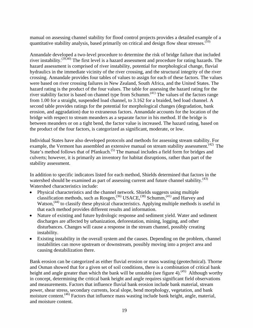
19

manual on assessing channel stability for flood control projects provides a detailed example of a quantitative stability analysis, based primarily on critical and design flow shear stresses.(10) Annandale developed a two-level procedure to determine the risk of bridge failure that included river instability.(39,40) The first level is a hazard assessment and procedure for rating hazards. The hazard assessment is comprised of river instability, potential for morphological change, fluvial hydraulics in the immediate vicinity of the river crossing, and the structural integrity of the river crossing. Annandale provides four tables of values to assign for each of these factors. The values were based on river crossing failures in New Zealand, South Africa, and the United States. The hazard rating is the product of the four values. The table for assessing the hazard rating for the river stability factor is based on channel type from Schumm.(41) The values of the factors range from 1.00 for a straight, suspended load channel, to 3.162 for a braided, bed load channel. A second table provides ratings for the potential for morphological changes (degradation, bank erosion, and aggradation) due to extraneous factors. Annandale accounts for the location of the bridge with respect to stream meanders as a separate factor in his method. If the bridge is between meanders or on a tight bend, the factor value is increased. The hazard rating, based on the product of the four factors, is categorized as significant, moderate, or low. Individual States have also developed protocols and methods for assessing stream stability. For example, the Vermont has assembled an extensive manual on stream stability assessment.(42) The State’s method follows that of Pfankuch.(5) The manual includes a field form for bridges and culverts; however, it is primarily an inventory for habitat disruptions, rather than part of the stability assessment. In addition to specific indicators listed for each method, Shields determined that factors in the watershed should be examined as part of assessing current and future channel stability.(43) Watershed characteristics include: • Physical characteristics and the channel network. Shields suggests using multiple

classification methods, such as Rosgen,(36) USACE,(38) Schumm,(41) and Harvey and Watson,(44) to classify these physical characteristics. Applying multiple methods is useful in that each method provides different results and information.

• Nature of existing and future hydrologic response and sediment yield. Water and sediment discharges are affected by urbanization, deforestation, mining, logging, and other disturbances. Changes will cause a response in the stream channel, possibly creating instability.

• Existing instability in the overall system and the causes. Depending on the problem, channel instabilities can move upstream or downstream, possibly moving into a project area and causing destabilization there.

Bank erosion can be categorized as either fluvial erosion or mass wasting (geotechnical). Thorne and Osman showed that for a given set of soil conditions, there is a combination of critical bank height and angle greater than which the bank will be unstable (see figure 4).(45) Although worthy in concept, determining the critical bank height and angle requires significant field observations and measurements. Factors that influence fluvial bank erosion include bank material, stream power, shear stress, secondary currents, local slope, bend morphology, vegetation, and bank moisture content.(46) Factors that influence mass wasting include bank height, angle, material, and moisture content.

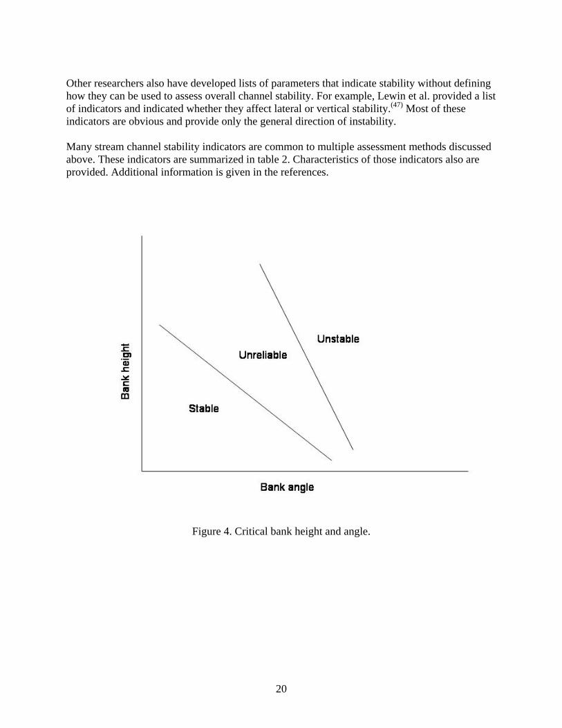
20

Other researchers also have developed lists of parameters that indicate stability without defining how they can be used to assess overall channel stability. For example, Lewin et al. provided a list of indicators and indicated whether they affect lateral or vertical stability.(47) Most of these indicators are obvious and provide only the general direction of instability. Many stream channel stability indicators are common to multiple assessment methods discussed above. These indicators are summarized in table 2. Characteristics of those indicators also are provided. Additional information is given in the references.

Figure 4. Critical bank height and angle.

21

Table 2. Summary of common indicators used in channel stability assessment methods.

Indicator Characteristics References

Boundary conditions Changes in loads to the stream, including water and sediment inputs. Causes channel to adjust. Amount and type of adjustment primarily based on channel type.

17, 20

Flow habit and flashiness

Ephemeral, intermittent, or perennial; flashiness; stream order. Flashy urban or ephemeral streams tend to be unstable relative to nonflashy perennial streams. Large ephemeral streams more unstable than first order.

3, 10, 48

Valley setting, confinement

Confinement by narrow valley, rock walls, or revetments limits lateral migration and may promote downcutting. 3

Channel pattern and type

Indicates energy in the system, propensity for lateral migration, processes on larger scale. 3, 11, 20, 37, 40, 41, 48, 49, 50

Entrenchment, incision

Indicated by levees, terraces, low width-to-depth ratio, confinement, exposed infrastructure. Indicates processes that have been occurring.

2, 20

Bed material

Size, uniformity, and packing are typical measurements and observations that indicate movement, armoring, and energy of the system. Fraction of sand and gravel can also indicate sediment transport characteristics.(51,52)

5, 10, 11, 30, 48, 49, 50, 51, 52, 53, 54, 55

Bar development

Indicators of bar stability include the relative bar size, bar material, and vegetation. For streams on higher slopes (> about 0.02) and low width-to-depth ratios < 12, bars are not typically evident.

3, 20

Bed and bank obstructions

Obstructions include rock outcrops, cohesiveness, grade control, bridge bed paving, debris jams, dikes or vanes, and revetments. They can cause flow diversions that erode beds and banks.

2, 5, 20

22

Table 2. Summary of common indicators used in channel stability assessment methods, continued.

Indicator Characteristics References

Bank material Layers/lenses, material size and sorting, and cohesiveness indicate the coherence of the material and resistance to erosion.

10, 56, 57, 58

Bank angle and height

Critical heights can be determined, greater than which the bank is susceptible to failure. Stable banks have low angles and heights.

5, 45, 57, 58

Bank and riparian vegetation

Woody vegetation helps maintain stability. The type, diversity, density, health, vertical orientation, and maturity of woody vegetation are indicators of stabilization effects. Rosgen includes root density.(37)

5, 7, 37

Bank cutting The relative amount of bare banks and root exposure along a bank indicate stability. 5, 20

Mass wasting Indicated by scalloping of banks, irregular channel width, tension cracks, slumping. 3, 5

23

STREAM CLASSIFICATION A stream classification scheme is a method of classifying a stream according to a set of observations. Streams are usually classified for the purpose of communication; a description of a stream by a classification gives the reader or audience an immediate picture of the appearance and condition of that stream channel and possibly its relationship to the surrounding flood plain and other streams in the system. More recently, classification schemes also are being used as a basis for channel restoration designs. There are a variety of classification schemes; the choice of scheme is problem dependent. Niezgoda and Johnson list 27 classification schemes devised over time, beginning in 1899, and a brief description of each.(59) Although the idea of classifying a stream may initially seem to be a trivial matter, the many complexities of stream configuration and planform often make classification difficult. In addition, classification schemes tend to force the stream into a category which may be useful for communicating the condition of a stream, but may be detrimental in that it may overlook certain unique or unusual characteristics of a stream. For example, few, if any, stream classification schemes include characteristics of streams in highly urbanized settings. Therefore, to use an available classification scheme, the urban stream is frequently forced into a particular classification. While this may communicate some characteristics of the stream, it ignores others. One of the most commonly used and useful classification schemes is stream order. The order of a stream describes the relationship of the stream to all other streams in the watershed. Streams that have no tributaries flowing into them are ranked as number one, or first-order streams. A second-order stream is one that is formed by the junction of two first-order streams or by the junction of a first- and a second-order stream. This ranking scheme is continued for all channels within the drainage basin. Stream order increases in the downstream direction, and only one stream channel can have the highest ranking. This process of ranking is a rather simple matter for a small drainage basin, but can become very difficult for a large, complex basin. Various stream characteristics have been related to stream order. For example, channel slope and channel length can be related to stream order in a given basin. First-order streams typically are steeper and shorter than second-order or higher streams. Fourth-order streams typically are relatively large, wide, low-gradient streams. This information can be useful in determining various characteristics about drainage basins, particularly large basins where extensive data gathering is impractical. Streams also can be classified according to other physical channel characteristics. These characteristics are qualitatively described by variables such as point bars, meanders and braiding, bank material, and valley slope. Brice and Blodgett developed a classification system for streams based on qualitative observations about the channel width, flow habit, flood plain, degree of sinuosity and braiding, development of point bars, bank material, and vegetative cover on the banks.(60) Rosgen developed a similar, but more extensive, stream classification scheme that has recently come into widespread use.(36,61) In this scheme, a stream is classified according to sinuosity, channel slope, bed material, entrenchment ratio, and width-to-depth ratio. The Rosgen scheme categorizes streams as six different types, A through G. Each type is associated with a range of slopes, width-to-depth ratios, sinuosities, and entrenchment. The streams are further subdivided according to the median size of the channel bed material. For example, a C5 stream is a low gradient, meandering stream with a high sinuosity and a sand bed.

24

Montgomery and Buffington developed a stream classification scheme that also has been used widely in recent years.(9) The stream type is based on the location within the watershed, the response to the sediment load, and several physical attributes. Table 3 provides the stream types and their characteristics. A primary advantage of using this method is that it is relatively simple and provides information on processes according to channel type. The channel types refer to natural, unmodified channels. USACE developed a method for classifying streams based on location and processes within a watershed.(10) Figure 5 depicts the stream types that are based on location. In addition, there are categories for arroyos, underfit (glaciated) streams, regulated streams, deltas, and modified channels. Classifying a given stream channel is entirely based on the descriptions given in figure 5. The advantage of this method is that it includes engineered or modified channels, which are common across the United States.

25

Table 3. Montgomery and Buffington stream classification system.(9)

Braided Dune-Ripple Pool-Riffle Plane-Bed Step-Pool Cascade Bedrock Colluvial

Typical Bed Material Variable Sand Gravel Gravel,

cobble Cobble, boulder Boulder N/A Variable

Bedform Pattern

Laterally oscillary Multilayered Laterally oscillary None Vertically

oscillary None N/A Variable

Reach Type Response Response Response Response Transport Transport Transport Source

Dominant Roughness Elements

Bedforms Sinuosity, bedforms

Bedforms, grains, LWD, sinuosity, banks

Grains, banks Bedforms, grains, large woody debris (LWD), banks

Grains, banks Boundaries Grains,

LWD

Dominant Sediment Sources

Fluvial, banks failure, debris flow

Fluvial, bank failure, inactive channel

Fluvial, bank failure, inactive channel, debris flows

Fluvial, bank failure, debris flows

Fluvial, hill slope, debris flow

Fluvial, hill slope, debris flow

Fluvial, hill slope, debris flow

Hill slope, debris flow

Sediment Storage Elements

Overbank, bedforms

Overbank, bedforms, inactive channel

Overbank, bedforms, inactive channel

Overbank, inactive channel

Bedforms Lee and Stoss sides of flow obstructions

N/A Bed

Typical Slope S < 0.03 S < 0.001 0.001 < S < 0.02 0.01 < S < 0.03

0.03 < S < 0.08

0.08 < S < 0.30 Variable S > 0.20

Typical Confinement Unconfined Unconfined Unconfined Variable Confined Confined Confined Confined

Pool Spacing (Channel Widths)

Variable 5 to 7 5 to 7 None 1 to 4 < 1 Variable Variable

26

Figure 5. USACE(10) stream classification system.

Mountain Torrents. High velocity streams on steep slopes with a drop-and-chute structure often achieved by obstacles such as large boulders or debris. These streams are subject to scour and degradation caused by flood events. Very steep slopes can lead to debris flows that produce substantial movement of boulders and gravels. Alluvial Fans. Occur usually in arid and semiarid lands where a stream flowing through a stream valley enters a flat area. The coarse sediment carried by the stream deposits in a delta-like configuration characterized by multiple channels subject to shifting. The chief stability problem is caused by the unpredictability of the flow paths, which may cause erosion and deposition in unexpected places. Braided Rivers. The main characteristic of these streams is a series of interlaced channels defined by bars and islands. Braided streams often occur in upper and middle zones of the watershed and usually involve gravel and cobbles, although braiding may also occur in sands. Scour and deposition often cause shifting of the main channel. Arroyos. Present in arid and semiarid lands, these are streams that remain dry most of the time and carry flow only during flood events. Discharge and sediment transport can be substantial during flow episodes. Incising channels, width enlargement, and deposition are typical problems associated with arroyos. Meandering Alluvial Rivers. These occur primarily in the middle and lower portion of the watershed. The planform of the stream is characterized by meanders that erode the streambank in the outer side of the bend and deposit material on the inner side. Meanders may migrate in the flood plain and can often become cutoff periodically when two bends advance toward each other and curvatures becomes severe. Cutoff meanders become isolated features called “oxbow lakes” that eventually fill with sediment. Traces of old meanders (scrolls) are easily distinguishable in aerial photographs. Measures that alter the supply of water or sediment have the potential to change cross sections, planforms, and gradients. Modified Streams. This term generical1y encompasses those streams whose natural configuration has been severely modified by human intervention. These modifications include straightening, channelizing, enlargement, and base level changes caused by regulation of the receiving stream. Increased runoff from surrounding development also introduces modifications. Regulated Streams. Regulation of tributaries by upstream reservoirs reduces flood flows and increases baseflow. These changes in the flow regime translate into reduced morphological activity. If regulation facilitates sediment deposition in the channel and vegetation growth, the stream cross section will be reduced. However, if the stream carries substantial sediment loads that become trapped in the reservoir, the stream may cause erosion downstream of the dam. Deltas. These features occur on flat slopes of the lower portion of the stream where it empties into relatively quiescent water such as the ocean or a lake. Sediment deposition due to reduced velocity forces the river to split into distributaries whose base level rises as the delta progresses into the water body. Deltas also exhibit the formation of natural levees along the distributaries. Underfit Streams. These are streams common in regions whose landscape formed as a result of glacial activity. Underfit streams occur in wide valleys formerly shaped and occupied by larger streams, usually the outlet to glacial lakes. Underfit streams are also found in abandoned riverbeds or channels downstream from reservoirs. Flat slopes, low velocities, and established vegetation make underfit streams generally stable. Cohesive Channels. These are channels cut in cohesive materials such as marine clays, silted lakes, and glacial till plains. In marine deposits, these streams behave somewhat like meandering alluvial streams, although the meanders are flatter, wider, more uniform, and usually more stable. In glacial till, the planform tends to be irregular.

27

PHYSIOGRAPHIC REGIONS The United States can be divided into eight major physiographic regions based on geologic and geomorphologic characteristics. The major regions can be further subdivided into subregions, for a total of 25 physiographic regions. The boundaries of these regions are not strictly defined. Rather, the regions are approximately mapped to provide a description of major physiographic changes across the country. Figure 6 shows these regions based on a map created by Fenneman and Johnson.(62) The regions and subregions are: • Region 1—Laurentian Highlands, including Superior Uplands. • Regions 2–3—Atlantic Plain, including Coastal Plain and Continental Shelf. • Regions 4–10—Appalachian Highlands, including Piedmont, Blue Ridge, Valley and Ridge,

St. Lawrence, Appalachian Plateau, New England, Adirondack. • Regions 11–13—Interior Plains, including Interior Low Plateau, Great Plains, Central

Lowlands. • Regions 14–15—Interior Highlands, including Ozark Plateaus, Ouachita Province. • Regions 16–19—Rocky Mountain System, including southern Rocky Mountains, Wyoming

basin, middle Rocky Mountains, northern Rocky Mountains. • Regions 20–22—Intermontane Plateaus, including Columbia Plateau, Colorado Plateau,

Basin and Range. • Regions 23–25—Pacific Mountain System, including Cascade-Sierra Mountains, Pacific

border, lower California. Physiographic regions provide natural divisions by which to investigate stream processes and erosion issues broadly. Thornbury defined a physiographic unit as an area of land with similar or uniform topographic characteristics, including altitude, relief, and type of landforms, that are distinctly different from other physiographic units.(63) Dietz suggested that the erosion and sedimentation processes and the rates of those processes also define the topography and landforms.(64) Several publications describe the landforms and underlying geologic structure of each of the physiographic regions listed above.(63,65,66) The landforms result from the combination of the underlying geologic structure and the erosion processes on the surface. Thus, gross characteristics of the streams can be summarized for each of the physiographic Provinces. Within each of these Provinces, however, there is a range of stream types due to variability in valley slope, sediment supply, and water discharge. In addition, changes to the stream channels through engineering of channels (straightening, clearing, widening, dredging) and removal of riparian vegetation also have tremendous impacts on the form that the channel will take. A number of studies supply evidence of the link between stream channel characteristics and physiographic region. Based on field observations and a detailed literature review, Graf characterized the physiographic Provinces and the stream types in each.(67) The recent activities in stream restoration have motivated a number of studies that attempt to characterize the morphologic characteristics of stream channels within a specific physiographic region. Most of these studies are focused on developing so-called regional equations that provide stream width and depth as a function of drainage area and/or bankfull discharge. These equations typically are developed within specific physiographic Provinces, thus providing additional evidence of common stream channel characteristics as a function of physiography. When comparing the

28

Figure 6. Physiographic map of the United States (after reference 66).

29

regional equations with other sites, it should be kept in mind that the data for the equations are almost always collected at stream gages, which means that the site is likely to be stable. Thus, a comparison of widths and depths obtained from these equations with those measured at other sites may indicate relative stability of the observed site. These studies and others are summarized below for streams in selected regions to illustrate the variation in streams from one region to another. Appalachian Highlands. Streams in this region are generally meandering and perennial; however, the pattern is greatly influenced by slope, geology, and bed materials.(68) In the higher elevations, the geology is generally (although with exceptions) more resistant material. Hack showed that slopes in the Shenandoah Valley are much steeper (about seven times steeper) than those in the Martinsburg, shale areas, while streams in the carbonate rock areas had slopes in between those of the Shenandoah Valley and Martinsburg, shale areas.(69) However, Hack also showed that the slopes of channels across the Appalachian region could be predicted by 18(d/AD)0.6(70), where AD is the drainage area d is the median size of the bed material. Channel pattern in this region is also controlled by bedrock. The bedrock exposures and rough terrain tends to create waterfalls and fast-moving streams across the region.(71) Regional equation parameters, developed by the U.S. Geological Survey for the Appalachian Plateau of New York, are given in table 5.(72) The equations resulted in a width-to-depth ratio of 16.5AD

0.09, which can be approximated as 16.5, since the exponent of 0.09 is quite small and has little effect on the width-to-depth ratio. Piedmont streams are moderately sloped, controlled by bedrock outcroppings.(71) Bed material is primarily sand and gravel.(73) A number of studies have determined the hydraulic geometry of Piedmont streams. The resulting regional equation parameters are given in table 4. Variation within the resulting width-to-depth ratios are significant, ranging from about 5.04 to 12.53. The range can be attributed to variability in levels of urbanization, land use, location within the Piedmont, and differences in observer identification of bankfull elevations. Coastal Plain. Streams are perennial and primarily meandering with limited reaches of braiding where channel slopes are higher and sediment loads are greater.(74) Oxbow lakes, back-swamps, and natural levees are common. Engineered dams and levees are also common to control flooding. Coastal Plain stream bottoms consist of more easily erodible material than the neighboring Appalachian Highlands.(71) Stream slopes are primarily gentle with bed material consisting of sand to fine gravel. Studies have been conducted in several eastern States to determine the hydraulic geometry of streams in the Coastal Plain region. Sweet and Geratz developed the set of regional equation parameters for North Carolina’s Coastal Plain, given in table 4.(75) Prestegaard found slightly different equations for width and depth, also given in table 4.(73) She determined average bed materials to be in the sand and gravel ranges with an average median sediment size of 8 millimeters (mm). She also found that, in general, Coastal Plain streams were deeper and narrower than Piedmont streams. This can be seen by comparing the width-to-depth ratios for each region. Great Plains and Central Lowlands. Streams in the Great Plains and Central Lowlands can be ephemeral, intermittent, or perennial. The Great Plains represent a depositional environment, deriving sediment from the mountains to the west. Deposited sediment is then reworked and moved through the channel system.(76) Channel morphology in the Midwestern United States has

30

been affected by water development projects. Several well-known geomorphic studies in the Great Plains have related channel geometry and hydraulic geometry sediment characteristics and flow discharge.(80,81) Both the Central Lowlands and the Great Plains, as well as portions of the Interior Lowlands, are covered with thick deposits of loess.(82) Simon and Rinaldi conducted reconnaissance studies at streams throughout the Midwest and determined that the combination of easily erodible soils and extensive human disturbance has produced thousands of miles of highly unstable streams.(82) Rocky Mountains. Local variations in geological setting and tectonics have significant control over fluvial processes and, thus, stream morphology.(83) Coarse-grained sediment is transferred from the mountains to the surrounding basins. Channels in the mountains are relatively steep and carry a coarse sediment load. In the adjacent basins, channels have lower gradients and transport finer grained materials that are derived, in part, from the coarser upstream load. Basin and Range. This Province is primarily arid to semiarid. Thus, rivers in the Basin and Range tend to be ephemeral or intermittent. Alluvial fans are common in the Basin and Range. They develop when sediment transported along steep, mountain channels deposits on shallower slopes at the base of the mountains. Streams in alluvial fans are typically highly unstable in terms of lateral position. One of the most outstanding characteristics of rivers in the Basin and Range is that drainage across most of the Province is internal.(84) Castro and Jackson developed regional equation parameters, given in table 4, for the upper Basin and Range based on measurements at 22 stream channels.(79) Pacific Coastal (California). The Pacific Coastal region in California is characterized by a wide variety of drainage types that include arroyos and alluvial fans.(85) Streams in both of these stream types tend to be unstable both laterally and vertically. Human alterations of stream channels in this region are widespread and have changed the erosion and depositional patterns. Streams may be ephemeral, intermittent, or perennial. Castro and Jackson developed regional equation parameters for this region, given in table 4.(79)

31

Table 4. Regional equation parameters for selected physiographic regions in the United States.

Reference Region a b c d f g i j w/y (Q) w/y (AD)

77 Piedmont – – – – 5.43 0.33 0.54 0.33 N/A 10.06

78 Piedmont 1.46 0.52 0.19 0.42 14.78 0.39 1.18 0.34 7.68 12.53

73 Piedmont 1.36 0.52 0.27 0.37 21.5 0.25 2.09 0.14 5.04 10.29

72 Appalachian Plateau – – – – 13.19 0.46 0.80 0.37 N/A 16.50

75 Coastal Plain 1.06 0.50 0.11 0.48 9.64 0.38 0.98 0.36 9.64 9.84

73 Coastal Plain 3.15 0.39 0.51 0.28 11.3 0.35 1.93 0.12 6.18 5.85AD0.23

79 Basin and Range 0.96 0.60 0.36 0.31 3.27 0.51 0.79 0.24 2.67Q0.3 4.14AD

0.27

79 Pacific Coastal 2.37 0.5 0.15 0.45 12.39 0.43 0.66 0.39 15.8 18.77

42 New England 2.65 0.47 0.62 0.23 10.18 0.50 1.22 0.25 4.08Q0.23 8.35AD0.25

w = aQb, y = cQd, w = fADg, y = iAD

j; w/y (width-to-depth) ratios are approximated as constants for w/y with very small exponents for either Q or AD The variables a-j are regression coefficients

33

3. FIELD OBSERVATIONS

Numerous stream-bridge intersections were observed across the United States to develop and test the stability assessment method. The streams were to reflect a broad range of stream types and physiographic regions; thus, 57 site visits were conducted in 13 physiographic regions and subregions, including Pacific Coastal, Basin and Range, Trans Pecos, southern Rocky Mountains, Great Plains, Central Lowlands, Interior Lowlands, Ozark-Ouachita Plateau, Appalachian Plateau, Valley and Ridge, Piedmont regions, and Atlantic Coastal Plain. In addition to collecting observations at streams covering a variety of erosion issues, sizes, and physiographic regions, the following criteria also were used in selecting appropriate sites: • All channels were alluvial or partially alluvial (occasional rock outcrops were acceptable). • Engineered (straightened or widened) channels were included, although manmade canals

were not. • The streams had to be wade-able or partly wade-able. • The streams and bridges had to be safely accessible. • A reasonable level of personal physical safety had to be satisfied. • The streams were located within a reasonable distance of the travel corridor. The data for each of the streams are summarized in tables 5–7. Streams that are named N# in table 5 are unnamed on topographic maps. Table 5 provides the locations and global positioning system (GPS) coordinates of the bridges, the physiographic Province, land use, and stream classification. Each of the channels was classified according to the Montgomery-Buffington scheme. The Montgomery-Buffington scheme does not include engineered or altered channels. However, this method is still useful as a basic descriptor of the primary processes in the stream (e.g., transport versus response) and is, therefore, included. To include altered streams, the USACE method(10) and a simple observation of channel pattern (based on both field observation and aerial photos) also were used to classify or categorize the stream types. The resulting stream type is provided as a combination of these methods in table 5. The Rosgen classification method was not considered because it is unnecessarily data intensive for the purposes of assessing channel stability in the vicinity of a bridge. Table 6 provides the bed and bar material, the percent of sand (Fs), and any controls observed in the banks or on the bed. Table 7 provides observations made on the banks, including vegetation, bank material, bank height, and any erosion characteristics. In the next section, observations made in each of the physiographic regions are described.

34

Table 5. River data summary.

GPS Location River Map Location

N. Latitude (deg)

W. Longitude(deg)

Physiographic Province

M-B/USACEClass* Land Use Channel

Pattern

1. Saline U.S. Rt. 183 22.5 kilometers (km) N of Hays, KS 39.0973 99.3055 Great Plains D/MA Cultivated Meandering

2. S. Fork Solomon R.

U.S. Rt. 283 1.6 km S of Hill City, KS 39.3506 50.8457 Great Plains D/MA-BR Cultivated Meandering to

braided

3. N. Rush Cr. State Route (S.R.) 71, S of Limon, CO 39.0609 103.7035 Great Plains D/MA Managed/grass Meandering

4. Arkansas R. S.R. 291, N of Salida, CO 38.6127 106.0618 Rocky Mtn. R/MA Natural/ cultivated Meandering

5. Tomichi Cr. S.R. 114, 12.9 km E of Gunnison, CO 38.5202 106.7852 Rocky Mtn. R/MA,MO Cattle pasture Meandering

6. Murietta Cr. Main St., Temecula, CA 33.4924 117.1499 Pacific Coastal D/MA-BR, MO Suburban Meandering

7. Jacalitos Cr. Jayne Ave., 9.7 km E of U.S. Interstate (I)-5 exit to Coalinga, CA

36.1369 120.2771 Pacific Coastal D/MA-BR Cattle grazing Meandering to braided

8. Dry Cr. Dry Creek Road, CA 38.4114 122.4513 Pacific Coastal C/MT- MA Wooded Irregular

9. Dutch Bill Cr. Bohemian Hwy., 9.7 km E of Oakville, Napa Valley, CA 38.4239 122.9569 Pacific Coastal R-C/MA-MT Wooded Irregular

10. Buena Vista Cr.

S.R. 58 1.6 km E of Buttonwillow, CA 35.3995 119.5321 Pacific Coastal B/MA-BR Cattle grazing Meandering to

braided

11. Mojave R. 1st Ave., Barstow, CA N/A N/A Basin and Range B/BR Rural/industrial Braided *C = cascade, S = step pool, P = plane bed, R = pool-riffle, D = dune-ripple, B = braided, MT = mountain torrent, MA = meandering, MO = modified, S.R = State Route, Cr. = Creek, R. = River

35

Table 5. River data summary, continued.

GPS Location River Map Location

N. Latitude (deg)

W. Longitude(deg)

Physiographic Province

M-B/USACEClass* Land Use Channel

Pattern

12. Rt. 66 Wash Rt. 66, E of Ludlow, CA 34.7160 116.1053 Basin and Range B/AR Natural Arroyo/braided

13. Sacramento Wash

S.R. 68, 27.4 km E of Lauchlin, AZ 35.2250 114.2800 Basin and Range R-B/MA-BR Rural/mining Meandering to

braided

14. Rio San Jose S.R. 6, 1.6 km S of I-40, Exit 126, NM 34.9675 107.1749 Trans Pecos R/MA,MO Grazed/natural Meandering,

channelized

15. Rio Puerco S.R. 6, 24.2 km E of Los Lunas, NM 34.7966 106.9905 Trans Pecos R/MA,MO Grazed/natural Meandering,

channelized

16. W. Elk Cr. E. Third St. (Rt. 66), W of Elk City, OK 35.4119 99.4522 Central Plains R/MA,MO Suburban, cattle Meandering,

channelized

17. Beaver Cr. U.S. Rt. 183, ~1.6 km N of Arapahoe, OK 35.5941 98.9602 Central Plains R/MA,MO Agricultural,

cattle Meandering

18. Brush Creek U.S. Rt. 62, 1.6 km E of Jacktown, OK 35.5068 96.9862 Central Plains R/MA Agricultural,

grazed Meandering

19. Unnamed U.S. Rt. 62, 1.6 km E of Boley, OK 35.4862 96.4594 Central Plains R/MA Natural, grazed,

rural Meandering

20. Little Skin Cr. U.S. Rt. 64, 1.6 km W of Muldrow, OK 35.3982 94.6211 Ozark-Ouachita

Highlands R/MA Natural, rural Meandering

21. Unnamed U.S. Rt. 64, at Dyer, AR 35.4964 94.1363 Ozark-Ouachita Highlands R/MA, MO Rural Meandering,

straightened

22. Little Cypress Cr.

S.R. 59, 1.6 km S of I-40, Exit 35 35.3402 89.5018 Coastal Plain R/MA Agricultural,

rural Meandering

*C = cascade, S = step pool, P = plane bed, R = pool-riffle, D = dune-ripple, B = braided, MT = mountain torrent, MA = meandering, MO = modified, S.R = State Route, Cr. = Creek, R. = River

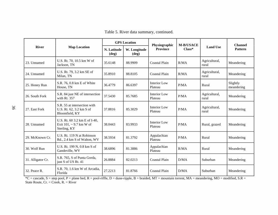
36

Table 5. River data summary, continued.

GPS Location River Map Location

N. Latitude (deg)

W. Longitude (deg)

Physiographic Province

M-B/USACEClass* Land Use Channel

Pattern

23. Unnamed U.S. Rt. 70, 10.5 km W of Jackson, TN 35.6148 88.9909 Coastal Plain R/MA Agricultural,

rural Meandering

24. Unnamed U.S. Rt. 79, 3.2 km SE of Milan, TN 35.8910 88.8105 Coastal Plain R/MA Agricultural,

rural Meandering

25. Honey Run S.R. 76, 0.8 km E of White House, TN 36.4779 86.6397 Interior Low

Plateau P/MA Rural Slightly meandering

26. South Fork S.R. 84 just NE of intersection with Rt. 357 37.5430 85.7685 Interior Low

Plateau P/MA Agricultural, rural Meandering

27. East Fork S.R. 55 at intersection with U.S. Rt. 62, 3.2 km S of Bloomfield, KY

37.8816 85.3029 Interior Low Plateau P/MA Agricultural,

rural Meandering

28. Unnamed U.S. Rt. 60 3.2 km E of I-40, Exit 101, ~ 9.7 km W of Sterling, KY

38.0443 83.9933 Interior Low Plateau P/MA Rural, grazed Meandering

29. McKnown Cr. U.S. Rt. 119 N at Robinson Rd., 2.4 km S of Walton, WV 38.5934 81.3792 Appalachian

Plateau P/MA Rural Meandering

30. Wolf Run U.S. Rt. 199 N, 0.8 km S of Gandeville, WV 38.6896 81.3886 Appalachian

Plateau R/MA Rural Meandering

31. Alligator Cr. S.R. 765, S of Punta Gorda, just S of US Rt. 41 26.8884 82.0213 Coastal Plain D/MA Suburban Meandering

32. Peace R. S.R. 70, 1.6 km W of Arcadia, Florida 27.2213 81.8766 Coastal Plain D/MA Suburban Meandering

*C = cascade, S = step pool, P = plane bed, R = pool-riffle, D = dune-ripple, B = braided, MT = mountain torrent, MA = meandering, MO = modified, S.R = State Route, Cr. = Creek, R. = River

37

Table 5. River data summary, continued.

GPS Location River Map Location

N. Latitude (deg)

W. Longitude (deg)

Physiographic Province

M-B/USACE Class* Land Use Channel

Pattern

33. Blackrock Run Stringtown Road off S.R. 25, N of Butler, MD 39.5437 76.7331 Piedmont R/MA

Suburban, agricultural, natural

Meandering

34. Indian Run Benson Mill Rd, off S.R. 25, N of Butler, MD 39.5691 76.7445 Piedmont R/MA Natural,

agricultural, rural Meandering

35. Middle Patuxent R. S.R. 108, N of Columbia, MD 39.2290 76.9173 Piedmont R/MA Natural, suburban Meandering

36. Hammond Branch

Stephens Rd., 2.4 km N of Laurel, MD 39.1318 76.8449 Coastal Plain R/MA Suburban,

agricultural Meandering

37. Atherton Tributary Seneca Dr., Columbia, MD 39.1871 76.8629 Piedmont R/MA Suburban Meandering

38. Stocketts Run Sands Rd., 4.8 km SW of Davidsonville, MD 38.8831 76.6638 Coastal Plain R/MA Natural, rural Meandering

39. Mill Stream Branch

S.R. 213, just S of Centreville, MD 39.0401 76.0722 Coastal Plain R6D/MA, MO Agricultural, rural Meandering

40. Kent County Tributary

S.R. 446 (Broadneck Rd.), SW of Chestertown, MD 39.2039 76.1235 Coastal Plain R6D/MA Agricultural Meandering

41. Morgan Creek Kennedyville Rd., 1.6 km E of Kennedyville, MD 39.2969 75.9845 Coastal Plain D/MA Agricultural Meandering

42. Little Elk Cr. Little Elk Rd, 1.2 km N of PA-MD line, 2.4 km S of Hickory Hill, PA

39.7271 75.9078 Piedmont P6R/ MA Agricultural, rural Meandering

*C = cascade, S = step pool, P = plane bed, R = pool-riffle, D = dune-ripple, B = braided, MT = mountain torrent, MA = meandering, MO = modified, S.R = State Route, Cr. = Creek, R. = River

38

Table 5. River data summary, continued.

GPS Location River Map Location

N. Latitude (deg)

W. Longitude (deg)

Physiographic Province

M-B/USACE Class* Land Use Channel

Pattern

43. Big Beaver Cr. Kuntz Mill Rd., off U.S. Rt. 222, 6.4 km N of Quarryville, PA

39.9411 76.2204 Piedmont R/MA Agricultural Meandering

45. Roaring Run PA Rt. 445, E of Nittany, PA 40.9810 77.5442 Ridge and Valley S/MT Natural Step-pool

44. Buffalo Run Fillmore Rd. (S.R. 3008) near State College, PA 40.8595 77.8769 Ridge and

Valley P/MA, MO Agricultural/ rural Meandering/ straightened

46. Potter Run S.R. 144 at Potters Mills, PA 40.8013 77.6257 Ridge and Valley S/MT Natural/rural Step-pool to

meandering

47. Bentley Cr. S.R. 4013 (Berwick Turnpike), about 1.6 km S of Bentley Creek, PA

N/A N/A Glaciated Appalachian Plateau

R/MA, MO Rural residential Meandering to braided

48. N 48 S.R. 58, 1.6 km W of Allegheny R., PA, S of I-80, 41.1340 79.6944 Appalachian

Plateau P, M/MT Natural/rural Plane bed, meandering

49. Reids Run S.R. 68, S of I-80 at Reidsburg, PA 41.1469 79.4020 Appalachian

Plateau P, M/MT Natural, agricultural, rural

Plane bed, meandering

50. Piney Creek S.R. 66, 0.8 km S of Limestone, PA 41.1281 79.3277 Appalachian

Plateau P, M Rural, agricultural Plane bed, meandering

51. Little Sandy Cr. S.R. 3011 at East Branch Station, PA 41.0327 79.0509 Appalachian

Plateau P, M Agricultural, rural Meandering

52. Trout Run S.R. 310, 1.6 km S of Reynoldsville, PA 41.0787 79.9016 Appalachian

Plateau P, M Natural, agricultural, rural Meandering

*C = cascade, S = step pool, P = plane bed, R = pool-riffle, D = dune-ripple, B = braided, MT = mountain torrent, MA = meandering, MO = modified, S.R = State Route, Cr. = Creek, R. = River

39

Table 5. River data summary, continued.

GPS Location River Map Location

N. Latitude (deg)

W. Longitude(deg)

Physiographic Province

M-B/USACE

Class* Land Use Channel

Pattern

53. Pootatuck R. Walnut Tree Hill Rd. near Sandy Hook, CT 41.4376 73.2702 New England P-R, MA Suburban, natural Meandering

54. Mill R. Judd Rd., N of Easton Reservoir, CT 41.3017 73.2760 New England P, MA, MO Natural Meandering,

straightened

55. Aspetuck R. Silver Hill Rd. at Easton, CT 41.2596 73.3249 New England P, MA, MO Natural, rural Meandering, straightened

56. W. Br. Saugatuck R. Stonebridge Rd. at Wilton, CT 41.1949 73.3875 New England P, MA Natural, suburban Meandering

57. Mianus R. June Rd., N of Merritt Pkwy, Stamford, CT 41.1048 73.5867 New England P, MO Natural, suburban Meandering,

straightened *C = cascade, S = step pool, P = plane bed, R = pool-riffle, D = dune-ripple, B = braided, MT = mountain torrent, MA = meandering, MO = modified, S.R = State Route, Cr. = Creek, R. = River

40

Table 6. River channel data.

River w/y Bed Controls

Bank Controls

Fs (%)

Bed Material

Bar Type

Bar Material

Bar Width

Bar Vegetation

1. Saline 20 None Abutments 80 Sand Alternate Sand 1/2 W Grasses

2. S. Fork Solomon R. 17 None Abutments 100 Sand Alternate Sand 1/3 W None/grass

3. N. Rush Cr. 15 None None 80 Sand None None N/A N/A

4. Arkansas R. 14 Gravel and cobble armor

Boulders, gravel armor, bridge abutments

30 Cobbles Point bars, midchannel

Very coarse gravel-cobbles

1/5 W Minimal

5. Tomichi Cr. 19 None Right bank riprapped 50 Very fine

gravel Midchannel (d/s only) Unknown < 1/5 W Shrubs

6. Murietta Cr. 9 None None 100 Sand Alternate Sand 1/2 W Heavily vegetated

7. Jacalitos Cr. 23 None Riprap at both bridge abutments

90 Sand Irregular/ combo Coarse sand

> 1/6, collectively very wide

Minimal

8. Dry Cr. 11 Boulders and occasional bedrock

Occasional bedrock and abutments

10 u/s Cobbles None u/s; Alternate/ irregular d/s

Sand 1/2–2/3 W None

9. Dutch Bill Cr. 10 None u/s Bridge

abutments 50 u/s Fine gravel Point bars Gravel 2/3 W None

10. Buena Vista Cr. 7.5– 15 None None 100 Sand Irregular Sand 1/2 W None

11. Mojave R. 6.7 None Piers, abutments

100 (fine) Sand Braided Sand Wide None

Fs = portion of sand, u/s = upstream, d/s = downstream, W = width, R. = River, Cr. = Creek

41

Table 6. River channel data, continued.

River w/y Bed Controls

Bank Controls

Fs (%)

Bed Material

Bar Type

Bar Material

Bar Width

Bar Vegetation

12. Rt. 66 Wash 10 Boulders

Boulders, bridge protection, abutments

70 Sand, gravel Irregular Sand, gravel Moderate None

13.Sacramento Wash 20 None

Bridge protection, piers, abutments

75 Clay, silt, sand, gravel

Irregular Sand and gravel Moderate None

14. Rio San Jose 5 None Riprap, piers,

abutments 70 Clay, silt, sand None N/A N/A N/A

15. Rio Puerco 16 None Clay/silt cliffs, piers, bank stabilization

20 Silt, clay, sand

Alternate, point Silt, clay Wide Grasses

16. W. Elk Cr. 9 Water line, debris None 100

(silt) Silt None N/A N/A N/A

17. Beaver Cr. < 4 None Bridge protection, soil blocks

100 (silt) Clay, silt Irregular Clay/silt Moderate None

18. Brush Creek 5 Boulders from

riprap

Bridge protection, bank stabilization

100 (silt, sand)

Clay, silt, sand Irregular Sand, silt,

little gravel None Narrow

19. Unnamed 15 Boulders Boulders, bridge protection, cliffs

100 Silt, sand Irregular Very fine sand Wide None, grasses

Fs = portion of sand, u/s = upstream, d/s = downstream, W = width, R. = River, Cr. = Creek

42

Table 6. River channel data, continued.

River w/y Bed Controls

Bank Controls

Fs (%)

Bed Material

Bar Type

Bar Material

Bar Width

Bar Vegetation

20. Little Skin Cr. 12 Beaver dams,

debris Bedrock, bridge protection

40 Sand, gravel Alternate bars Gravel Grasses,

shrubs Moderate

21. Unnamed 5 Debris Bars, debris 80 Silt, sand, gravel

Only under bridge Sand N/A N/A

22. Little Cypress Cr. 9 Few boulders

Bridge abutments and pier

80 Sand w/ silt, gravel Irregular Sand Narrow None

23. Unnamed 9 Bridge protection

Debris, bridge protection 100 Sand Irregular Sand Wide None

24. Unnamed 9 Grade control Bridge protection, piers

100 Sand Irregular d/s only (u/s pooled)

Sand Wide None

25. Honey Run 12 Outcrop Piers, bars 30 Gravel Alternate Gravel Narrow Grass/none

26. South Fork 9 None Piers 30 Gravel None N/A N/A N/A

27. East Fork 9 Boulders, gravel armor

Bridge protection 50 Sand,

gravel None N/A N/A N/A

28. Unnamed 12 Occasional bedrock, boulders

Occasional bedrock, abutments

20Sand, gravel, cobbles

None N/A N/A N/A

29. McKown Cr. 6 Gravel armor Bridge protection 10 Gravel None N/A N/A N/A

Fs = portion of sand, u/s = upstream, d/s = downstream, W = width, R. = River, Cr. = Creek

43

Table 6. River channel data, continued.

River w/y Bed Controls

Bank Controls

Fs (%)

Bed Material

Bar Type

Bar Material

Bar Width

Bar Vegetation

30. Wolf Run 5–8

Gravel armor, occasional bedrock, grade control at bridge

Clumps of failed bank material 10 Gravel

Irregular (mostly from failure material)

Gravel Moderate None

31. Alligator Cr. 24 None

Confined left bank concrete wall or rock lined

18 Silt None N/A N/A N/A

32. Peace R. 20 None

Gravel armor (bank protection), bridge riprap, debris

100 Very fine sand

Irregular/ combination

Very fine sand Wide, 1/2 W Grasses, reeds,

trees

33. Blackrock Run 5.5–17 Bedrock Bedrock,

abutments 65 Sand, gravel Irregular Sand, gravel Narrow None

34. Indian Run 5 Debris Bridge riprap, abutments, fiber logs, debris

50Sand, gravel, cobbles

Irregular Sand, gravel Wide Grasses

35. Middle Patuxent R. 16 Gravel

armor Bedrock, gabions, riprap at bridge

20 Sand, gravel Mid, point Sand, gravel Narrow None

36. Hammond Branch 7 Boulders

Bridge protection, abutments, riprap

60 Sand, gravel None N/A N/A N/A

Fs = portion of sand, u/s = upstream, d/s = downstream, W = width, R. = River, Cr. = Creek

44

Table 6. River channel data, continued.

River w/y Bed Controls

Bank Controls

Fs (%)

Bed Material

Bar Type

Bar Material

Bar Width

Bar Vegetation

37. Atherton Tributary 16 Bedrock,

boulders Boulders, abutments 40

Sand, gravel, boulders

Irregular Sand Narrow None

38. Stocketts Run 16 None Abutments 50 Sand,

gravel Point Sand, gravel Moderate None

39. Mill Stream Branch 13–16 None Abutments, debris 100 Sand Alternate Sand Narrow None

40. Kent County Tributary

3 None Abutments, concrete slabs 80 Silt, sand,

gravel Irregular Silt, sand Wide Grasses

41. Morgan Cr. 10 None Riprap, abutments 80 Silt, sand None N/A N/A N/A

42. Little Elk Cr. 20 Boulders

Bedrock, boulders, bridge protection, abutments

20

Sand, gravel, cobbles, boulders

Point Gravel, cobbles Narrow None/grasses

43. Big Beaver Cr. 20–29 Gravel

armor (d/s) None 20Silt, sand, gravel, cobbles

Midchannel (u/s), point (d/s)

Silt (u/s), sand, gravel (d/s)

Wide None

44. Buffalo Run 10

Gravel armor, u/s weir

Bridge protection 30 Sand, gravel

None N/A N/A N/A

45. Roaring Run 20

Boulders, riprap from failed bridge protection

Bridge protection, bank stabilization 10

Gravel, cobbles, boulders

Alternate (d/s only; u/s step-pool)

Gravel, cobbles Moderate None

Fs = portion of sand, u/s = upstream, d/s = downstream, W = width, R. = River, Cr. = Creek

45

Table 6. River channel data, continued.

River w/y Bed Controls

Bank Controls

Fs (%)

Bed Material

Bar Type

Bar Material

Bar Width

Bar Vegetation

46. Potter Run 15 Gravel/cobble armor

Bridge abutments, bank stabilization

30Sand, gravel, cobbles

None N/A N/A N/A

47. Bentley Cr. 32 None Abutments 60 Gravel Point, midchannel Gravel 1/4–2/3 W None

48. N 48 15 Gravel/cobble armor

Boulders, abutments, bank stabilization

10 Gravel, cobbles None N/A N/A N/A

49. Reids Run 15 Gravel/cobble armor, boulders

Boulders, abutments 10

Gravel, cobbles, boulders

None N/A N/A N/A

50. Piney Creek 10 Gravel armor

Bridge protection, abutments, bank stabilization

< 20 Gravel, cobbles Point bar Gravel Moderate None

51. Little Sandy Creek 18 Gravel armor Abutments < 20

Gravel, cobbles, boulders

Midchannel Gravel Grasses Narrow

52. Trout Run 10 Gravel armor Bridge protection, abutments

30 Gravel, cobbles None N/A N/A N/A

53. Pootatuck R. 28

Bedrock, boulders, gravel armor

Boulders, abutments 10

Gravel, cobbles, boulders

Irregular Gravel, cobbles Narrow None

Fs = portion of sand, u/s = upstream, d/s = downstream, W = width, R. = River, Cr. = Creek

46

Table 6. River channel data, continued.

River w/y Bed Controls

Bank Controls

Fs (%)

Bed Material

Bar Type

Bar Material

Bar Width

Bar Vegetation

54. Mill R. 13 Gravel armor, beaver dam d/s

Abutments 50 Sand, gravel Alternate d/s Sand, gravel Narrow None

55. Aspetuck R. 19 Gravel riffles

Boulders, bridge protection, bank stabilization

60 Sand, gravel

Alternate d/s (minor) Sand Narrow None

56. W. Br. Saugatuck R. 45 Boulders

Boulders, abutments, debris jams, islands

40Sand, gravel, cobbles

Midchannel, islands

Sand, gravel, cobbles Moderate Shrubs, trees

57. Mianus R. 13 Gravel armor (d/s of dam)

Boulders, abutments, bank stabilization

40 Gravel, cobbles None N/A N/A N/A

Fs = portion of sand, u/s = upstream, d/s = downstream, W = width, R. = River, Cr. = Creek

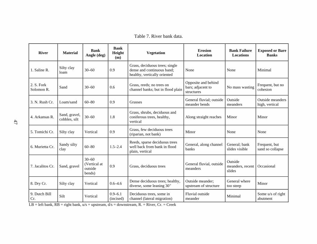
47

Table 7. River bank data.

River Material Bank Angle (deg)

Bank Height

(m) Vegetation Erosion

Location Bank Failure

Locations Exposed or Bare

Banks

1. Saline R. Silty clay loam 30–60 0.9

Grass, deciduous trees; single dense and continuous band; healthy, vertically oriented

None None Minimal

2. S. Fork Solomon R. Sand 30–60 0.6 Grass, reeds; no trees on

channel banks; but in flood plain

Opposite and behind bars; adjacent to structures

No mass wasting Frequent, but no cohesion

3. N. Rush Cr. Loam/sand 60–80 0.9 Grasses General fluvial; outside meander bends

Outside meanders

Outside meanders high, vertical

4. Arkansas R. Sand, gravel, cobbles, silt 30–60 1.8

Grass, shrubs, deciduous and coniferous trees, healthy, vertical

Along straight reaches Minor Minor

5. Tomichi Cr. Silty clay Vertical 0.9 Grass, few deciduous trees (riparian, not bank) Minor None None

6. Murietta Cr. Sandy silty clay 60–80 1.5–2.4

Reeds, sparse deciduous trees well back from bank in flood plain, vertical

General, along channel banks

General; bank slides visible

Frequent, but sand so collapse

7. Jacalitos Cr. Sand, gravel 30–60 (Vertical at outside bends)

0.9 Grass, deciduous trees General fluvial, outside meanders

Outside meanders, recent slides

Occasional

8. Dry Cr. Silty clay Vertical 0.6–4.6 Dense deciduous trees; healthy, diverse, some leaning 30E

Outside meander; upstream of structure

General where too steep Minor

9. Dutch Bill Cr. Silt Vertical 0.9–6.1

(incised) Deciduous trees, some in channel (lateral migration)

Fluvial outside meander Minimal Some u/s of right

abutment LB = left bank, RB = right bank, u/s = upstream, d/s = downstream, R. = River, Cr. = Creek

48

Table 7. River bank data, continued.

River Material Bank Angle (deg)

Bank Height

(m) Vegetation Erosion

Location Bank Failure

Locations Exposed or Bare

Banks

10. Buena Vista Cr. Sand/silt 60–90 0.6 Sparse shrubs General, irregular Slides in sand Frequent

11. Mojave R. Sand 60–90 1.8 None General Continual slides Continual

12. Rt. 66 Wash

Clay, silt, sand 70–90 0.6–1.8 None General Frequent Continual

13. Sacramento Wash

Clay, silt, sand, gravel 60–90 0.9 Few shrubs General Frequent slides,

slumps Continual

14. Rio San Jose

Clay, silt, sand 60–90 1.8 Desert shrubs Outside meanders,

general Outside meanders Continual

15. Rio Puerco Clay, silt 80–90 1.5 Grasses, shrubs (desert) Outside meanders, general

Outside meanders Continual

16. W. Elk Cr. Clay, silt 70–90 1.5 Grasses, shrubs, few trees General Where hoof damage, steep banks

Continual

17. Beaver Cr. Silt 90 2.4 Grasses, few bushes General Both banks—overheightened Continual

18. Brush Creek Silt 80 1.2–9.1

(top) Sparse trees General Minor, both banks Continual

19. Unnamed Clay, silt, sand 40–60 1.2–4.6 Sparse trees, grass, shrubs Outside meander bends RB Frequent

20. Little Skin Cr. Clay, silt 60 1.5 Grass, shrubs, trees (moderately

dense) Outside meander bend, general Mostly d/s Occasional

LB = left bank, RB = right bank, u/s = upstream, d/s = downstream, R. = River, Cr. = Creek

49

Table 7. River bank data, continued.

River Material Bank Angle (deg)

Bank Height

(m) Vegetation Erosion

Location Bank Failure

Locations Exposed or Bare

Banks

21. Unnamed Clay, silt (main), sand 70–90 0.9 Grass, shrubs, dense trees General None Minor

22. Little Cypress Cr. Clay, silt 90 0.9–3.7 Grass, dense trees General Outside bend Continuous

23. Unnamed Clay, silt, sand 80 2.4 Grass, dense trees General, outside bends

General—overheightened banks

Frequent

24. Unnamed Clay, silt 60–70 4.6 (levee) Grass, dense trees General None Occasional

25. Honey Run Clay, silt 60–90 0.9–1.8 (top of mass wasting)

Grass, dense trees General Along RB, especially where vegetation removed

Occasional

26. South Fork Clay, silt 70–80 2.4 Shrubs, sparse trees General Along both banks Frequent

27. East Fork Clay, silt 70 1.2 Grass Outside bend, general None Occasional

28. Unnamed Clay, silt 60–90 0.8 Shrubs, dense trees General (minor u/s) None Occasional

29. McKown Cr. Clay, silt 60–90 1.2 (u/s),

0.8 (d/s) Grass u/s, d/s grass on left bank, one row of trees on right General U/s only along

banks Occasional

30. Wolf Run Clay, silt, gravel 60–90 1.2 Grass General, outside, inside

bends Both banks Frequent

31. Alligator Cr. Silt, sand LB vertical,

RB moderate 0.8 LB grass, RB dense trees LB none (concrete), RB outside meander bend (minor)

None None

LB = left bank, RB = right bank, u/s = upstream, d/s = downstream, R. = River, Cr. = Creek

50

Table 7. River bank data, continued.

River Material Bank Angle (deg)

Bank Height

(m) Vegetation Erosion

Location Bank Failure

Locations Exposed or Bare

Banks

32. Peace R. Sand Steep outside bend, moderate elsewhere

3 Dense trees Opposite bar, outside meander bends

Left bank, outside bends Minor both banks

33. Blackrock Run

Clay, silt, sand 50–80 0.9–2.7 Shrubs, trees Outside meander,

opposite bar General—overheightened banks

Occasional

34. Indian Run Clay, silt 40–80 0.8–1.8 Sparse trees LB, grass RB General, opposite obstructions

RB where no vegetation Occasional

35. Middle Patuxent R. Clay, silt 40–60 1.5–1.8 Shrubs, dense trees in good

condition Outside meander bends, general

Limited on RB where high banks slough

Frequent on both banks

36. Hammond Branch Clay, silt 60–80 1.5 Grasses, sparse trees, falling

into stream, poor condition Outside meander, general Minor Continuous

37. Atherton Tributary Clay, silt 60–80 2.5-6 Sparse trees LB, dense trees RB,

falling trees both banks Outside meander None u/s, RB d/s where trees removed

Occasional

38. Stocketts Run Clay, silt

30–50, 80–90 outside bends

0.8–1.8 Shrubs, dense trees, falling on either side

Outside meander, general None Frequent

39. Mill Stream Branch Clay, silt 40–60 0.9–2.4 Sparse falling trees LB, dense

falling trees RB General None Occasional

LB = left bank, RB = right bank, u/s = upstream, d/s = downstream, R. = River, Cr. = Creek

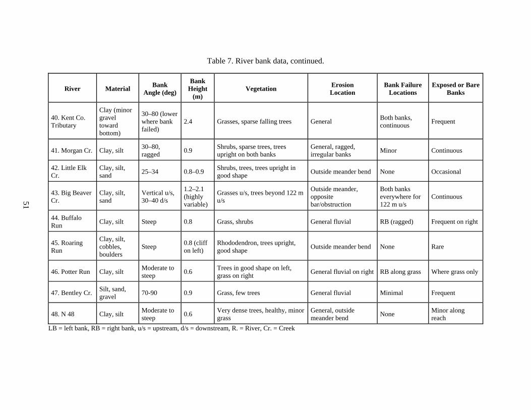
51

Table 7. River bank data, continued.

River Material Bank Angle (deg)

Bank Height

(m) Vegetation Erosion

Location Bank Failure

Locations Exposed or Bare

Banks

40. Kent Co. Tributary

Clay (minor gravel toward bottom)

30–80 (lower where bank failed)

2.4 Grasses, sparse falling trees General Both banks, continuous Frequent

41. Morgan Cr. Clay, silt 30–80, ragged 0.9 Shrubs, sparse trees, trees

upright on both banks General, ragged, irregular banks Minor Continuous

42. Little Elk Cr.

Clay, silt, sand 25–34 0.8–0.9 Shrubs, trees, trees upright in

good shape Outside meander bend None Occasional

43. Big Beaver Cr.

Clay, silt, sand

Vertical u/s, 30–40 d/s

1.2–2.1 (highly variable)

Grasses u/s, trees beyond 122 m u/s

Outside meander, opposite bar/obstruction

Both banks everywhere for 122 m u/s

Continuous

44. Buffalo Run Clay, silt Steep 0.8 Grass, shrubs General fluvial RB (ragged) Frequent on right

45. Roaring Run

Clay, silt, cobbles, boulders

Steep 0.8 (cliff on left)

Rhododendron, trees upright, good shape Outside meander bend None Rare

46. Potter Run Clay, silt Moderate to steep 0.6 Trees in good shape on left,

grass on right General fluvial on right RB along grass Where grass only

47. Bentley Cr. Silt, sand, gravel 70-90 0.9 Grass, few trees General fluvial Minimal Frequent

48. N 48 Clay, silt Moderate to steep 0.6 Very dense trees, healthy, minor

grass General, outside meander bend None Minor along

reach LB = left bank, RB = right bank, u/s = upstream, d/s = downstream, R. = River, Cr. = Creek

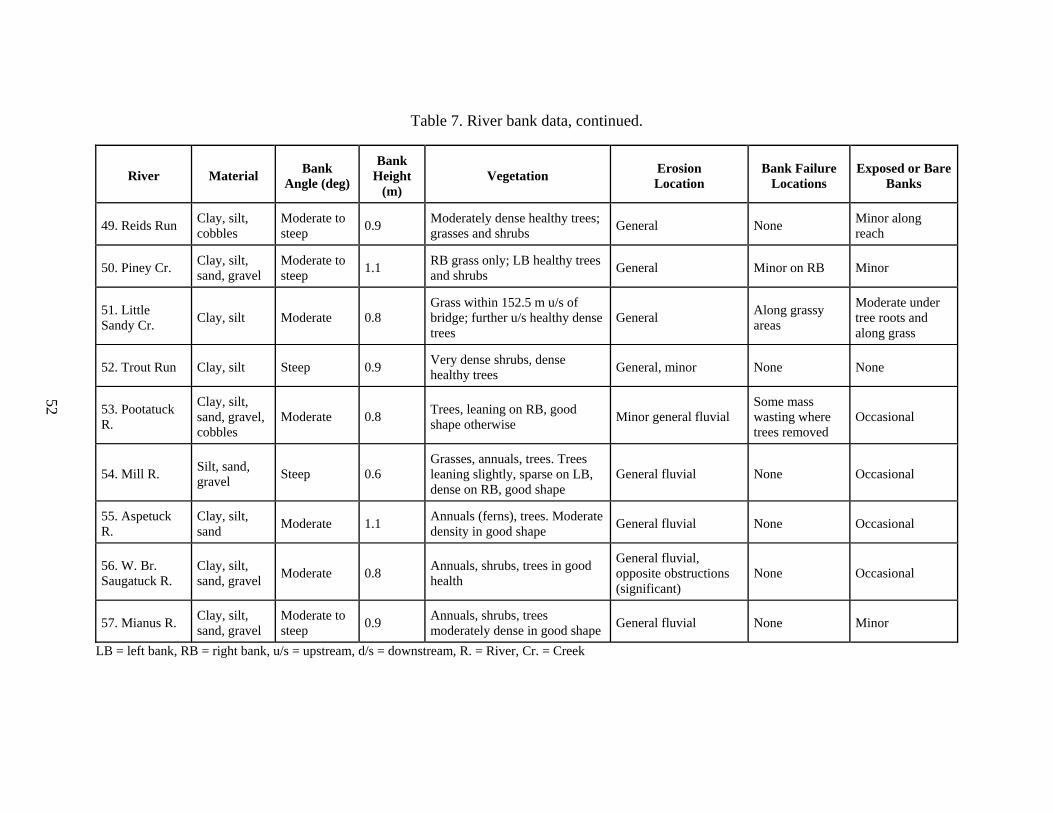
52

Table 7. River bank data, continued.

River Material Bank Angle (deg)

Bank Height

(m) Vegetation Erosion

Location Bank Failure

Locations Exposed or Bare

Banks

49. Reids Run Clay, silt, cobbles

Moderate to steep 0.9 Moderately dense healthy trees;

grasses and shrubs General None Minor along reach

50. Piney Cr. Clay, silt, sand, gravel

Moderate to steep 1.1 RB grass only; LB healthy trees

and shrubs General Minor on RB Minor

51. Little Sandy Cr. Clay, silt Moderate 0.8

Grass within 152.5 m u/s of bridge; further u/s healthy dense trees

General Along grassy areas

Moderate under tree roots and along grass

52. Trout Run Clay, silt Steep 0.9 Very dense shrubs, dense healthy trees General, minor None None

53. Pootatuck R.

Clay, silt, sand, gravel, cobbles

Moderate 0.8 Trees, leaning on RB, good shape otherwise Minor general fluvial

Some mass wasting where trees removed

Occasional

54. Mill R. Silt, sand, gravel Steep 0.6

Grasses, annuals, trees. Trees leaning slightly, sparse on LB, dense on RB, good shape

General fluvial None Occasional

55. Aspetuck R.

Clay, silt, sand Moderate 1.1 Annuals (ferns), trees. Moderate

density in good shape General fluvial None Occasional

56. W. Br. Saugatuck R.

Clay, silt, sand, gravel Moderate 0.8 Annuals, shrubs, trees in good

health General fluvial, opposite obstructions (significant)

None Occasional

57. Mianus R. Clay, silt, sand, gravel

Moderate to steep 0.9 Annuals, shrubs, trees

moderately dense in good shape General fluvial None Minor

LB = left bank, RB = right bank, u/s = upstream, d/s = downstream, R. = River, Cr. = Creek

53

PHYSIOGRAPHIC REGIONAL OBSERVATIONS Thirteen physiographic regions and subregions were included in the data set. A wide variety of land uses were observed in the various regions, including natural, agricultural, grazed, rural, and suburban. Width-to-depth ratios also varied widely, from 5 to 24. As expected, the largest ratios were associated with braided or semibraided channels. Very low width-to-depth ratios were associated with incised streams or those that had been engineered. Bed materials varied from very fine materials (silt and very fine sand) in the Midwest and coastal areas to coarser materials mostly associated with higher elevation streams. Bank materials varied widely. For example, the banks of the streams in the Central Plains tend to be made up of fine loess and silt deposits, which erode easily. In the Appalachian Plateau region, in contrast, the bank materials are far more cohesive and tend to be less susceptible to high erosion rates even when bank vegetation was limited. Although stream types vary widely within any of the physiographic regions, certain common characteristics were observed. A general summary of those observations is given here. The photos of the sites are organized by physiographic region in appendix A. Many, but not all, of them are referred to in the discussion below. Pacific Coastal

There are two striking features of stream channels within the border and lower Californian subregions of the Pacific Coastal region (see appendix A). The first is the wide diversity in types of channels. Streams range from perennial, cascading channels to arroyos. The second feature common to most streams in these subregions is the frequency of human interference and alteration. The channel bed material in most of the streams (other than first-order streams) was predominantly fine-to-medium sand, while the channel banks were sandy. The average width-to-depth ratio was 12.1. The streams tend to be very high energy; they are typically ephemeral, so they carry water only when there is rainfall. Many of these streams (and arroyos) tend to be naturally unstable, particularly in the lateral direction, and have relatively high width-to-depth ratios. Because of the high degree of channel instability and flash flooding in this region, many, if not most, of the channels in suburban to urban settings were either concrete lined or at least heavily armored with rock. Channels in the outlying areas were unlined. Intermontane

Observations at bridge-stream intersections were collected in the Basin and Range, Colorado Plateau, and Trans Pecos subregions within the Intermontane physiographic region. Many channels within the Colorado Plateau are bedrock or semialluvial channels in which stability is a function of bedrock erosion. In the Basin and Range, however, where the climate is arid to semiarid over much of the area, the streams are ephemeral with high energy, flashy flows (see appendix A). The energy of these streams combined with the highly erosion-prone sand beds and banks creates unstable channels, particularly at bridges. Due to the high sediment load carried by these streams, the width-to-depth ratios are relatively high, with an average of 25.0. Streams in the Trans Pecos region (see appendix A) tend to have high, steep banks or valley walls, which create valley side failures and subsequent failure material to the stream. The bed materials are sand, and banks are comprised of a mix of noncohesive materials, primarily sand, with minor

54

amounts of cohesive silts and clays. The predominant bank vegetation was desert shrubs, and mass wasting was a common form of erosion. The average width-to-depth ratio was 10.5. Rocky Mountain System

The southern Rocky Mountains were visited in this region (see appendix A). The channels contain large bed and bank material. The streams tend to be stable, transport streams that are less disturbed by human activities than in other physiographic regions. Stream channel banks are a mix of cohesive silts and clays and noncohesive gravels and larger materials. The average width-to-depth ratio was 16.5. Interior Plains

Three subregions—the Great Plains, Central Lowlands, and Interior Lowlands—were visited within the Interior Plains. In the Great Plains (see appendix A), vegetation in riparian areas and in the flood plains was thick, lush, and dense, except where cattle were permitted to graze. The channel beds were composed of more than 70 percent sand. Bank material was noncohesive silt, loam, and sand, but the thick vegetation helped to keep banks stable. The average width-to-depth ratio was 17.3. Erosion processes within the stream channels are primarily fluvial; observed channel banks were not sufficiently high to create significant mass wasting. Slow to moderate degradation occurred where cattle grazing was permitted. The Central Lowlands (see appendix A) had silt and loess banks that eroded easily. Many of the streams observed had been straightened in addition to having extensive hoof and/or grazing damage. The channel beds degrade rapidly since the bed material is predominantly silt with some clay and sand. The silt banks then become overheightened, and mass failures result. High, failing banks were common even where a wider riparian buffer existed, but the rate of failure was slower (for example, see figure 7). The average width-to-depth ratio was much lower than that observed in the Great Plains, with an average of 8.3. This may be due in part to channel modifications, such as straightening. Streams in the Interior Lowlands (see appendix A) seemed less fragile than those in the Central Lowlands due to larger bed material (sand and gravel) and more cohesive materials in their banks (clay and silt). However, where vegetation had been removed, banks failed even when they were not greatly overheightened (see figure 8). A single row of trees in the riparian areas slowed bank failure dramatically. These streams tend to have a low width-to-depth ratio, with an average of about 10.5, and remain stable even when the surrounding land has been disturbed. This may be due to the existence of rock outcrops in the beds and banks. Interior Highlands

In the combined Ozark-Ouachita Plateau (see appendix A), bed material was larger, containing some gravel. The bank material contains a significant percentage of cohesive clays. Natural erosion occurred at bends with increased mass wasting at bends where vegetation had been removed. Overheightened banks remained stable when more than one row of trees was in place. The average width-to-depth ratio was 8.5.

55

Appalachian Highlands

Within the Appalachian Highlands, the Appalachian Plateau, Valley and Ridge, and Piedmont regions were visited. In the Appalachian Plateau (see appendix A), bed material was coarser (mainly very coarse gravel to cobbles), with bank material composed of cohesive clay, silt, and minor sand. Critical bank heights appeared to be about 1.5 to 1.8 m, which result in low width-to-depth ratios. For the sites visited, the average ratio was 11.0. Watersheds are heavily forested where vegetation is undisturbed. Stream channel erosion and destabilization occurs through removal of vegetation and/or channel straightening. Overheightened banks may fail, but heal quickly if vegetation is allowed to re-establish; thus, stability tends to be fair at worst. Stream channels within the Piedmont region (see appendix A) had cohesive banks that could stand at high angles without failure. Bank vegetation, if undisturbed, was dense and provided bank stability with about one river width of woody vegetation. Banks with angles steeper than about 60E tended to have leaning or fallen trees. The potential for debris jams is high. Occasional bedrock outcropping was noted at all streams that were visited. Bed material was sand and gravel with occasional larger material. The average width-to-depth ratio was 15.3. The Valley and Ridge region of the Appalachian Highlands is comprised of a series of ridges separated by stream valleys. The streams in this region are often very steep, especially coming down from the ridges (see appendix A). Cascade and step-pool morphologies are common. Thus, bed materials are commonly large, such as cobbles and boulders, and often armor the bed. Banks are cohesive clays and silts with some larger materials mixed in, strongly held together by the lush vegetation found in this area. Disturbance to the banks by removal of vegetation may result in ragged, scalloped banks, but erosion of the banks is typically at a relatively slow rate. The average width-to-depth ratio was 15.0.

Figure 7. Failing banks in the Central Lowlands.

56

Figure 8. Failing banks in the Interior Lowlands. Coastal Plain

The Coastal Plain covers a very large area of the Atlantic and Gulf coastal areas (see figure 6). Sites were visited along both the Atlantic and Gulf coasts (see appendix A). In both of these areas, researchers observed moderate rates of bed degradation and bank failure. A buffer of at least one river width appeared to be sufficient in most locations to keep banks stable. Where undisturbed, lush vegetation on the banks held the banks in place, resulting in excellent stability, even when banks were nearly vertical. Bed material is typically sand with minor amounts of small gravel, and banks are cohesive with clay, silt, and minor amounts of sand. Because of the cohesive banks, strong vegetative resistance, and degradation, width-to-depth ratios tended to be rather low. Streams in this region are often sluggish due to low slopes and backwater from the bays or estuaries into which they flow. Where banks or the flood plain are disturbed, debris jams are frequent. The average width-to-depth ratios were much lower in the Gulf area (9.0) than in the Atlantic area (13.5). New England

All of the streams visited in the New England region were located in Connecticut. At all streams, the banks were heavily vegetated with large woody vegetation, providing tremendous stability to the streambanks. The bank materials typically were comprised of some cohesive materials combined with silt, sand and, in some places, gravel and larger particles. The bed materials in the New England region are considerably larger than in the Atlantic Coastal Plain to the south. The sand, gravel, and cobble beds were often armored; the width-to-depth ratios reflected this armored condition with an average value of 24. The channels were all meandering, but with beds transitional between plane beds and pool-riffle beds.

57

General Observations of Streams at Bridges

Channel stability is a function of levels of disturbance to the water and sediment discharges, and susceptibility of the channels to change. In every physiographic region, the disturbance that caused the greatest damage to the streams was the combination of cattle activity, vegetation removal, and channel straightening. The combined impact of these activities was worst where cattle had direct access to streams. Also, susceptibility of the channel banks to erosion significantly impacted the level of damage. Figures 9 and 10 provide examples of this combination of disturbances. All vegetation has been removed either through farming practices or by cattle grazing. The channel apparently had been straightened to provide better drainage and to maximize land for farming. Not only are cattle grazing in this area, but also they have direct access to the stream. Hoof damage is extensive. The combined disturbances have resulted in stream channel destabilization; the channel bed elevation has degraded and the banks have become overheightened and steepened. Figure 10 shows the eroding channel beneath the single-span bridge. In many cases, maintaining a riparian buffer of an appropriate width is all that is needed to preserve channel stability. As discussed in the descriptions of the streams channels across the physiographic regions, some regions require only a single row of trees to help maintain stability, while others require a much greater width. This is due to bank materials and the susceptibility of the banks to failure. In the cases where channels are degrading because of channel straightening, cattle grazing, and urbanization effects, a vegetation buffer may not be enough to maintain stability. When the channel degrades, banks can become overheightened and fail through mass wasting. In this case, vegetation may help to slow the rate of failure, but usually cannot prevent collapse of the banks.

Figure 9. Stream impacts due to disturbances, including hoof damage, vegetation removal, and channel straightening.

58

Figure 10. Impacts of disturbances at bridge (from figure 9). Another observation that was frequently made at sites in all physiographic regions was that there was often a distinct change in channel stability upstream and downstream of the bridges. This was caused in every case by a change in property management, as it is common for a road (and, thus, a bridge) to divide property ownership. As an example, unnamed stream N 28 is wooded upstream, with a healthy wide band of upright trees keeping the banks stable (see figure 11). Immediately downstream of the bridge, all trees and other vegetation have been removed, resulting in destabilization of the banks (see figure 12). Aerial photos were examined for each of the sites using http://terraserver-usa.com (these photos are not included in the report because they are readily available online). The photos were examined to check a larger view of the river, specifically looking at land use in the watershed and flood plain, construction areas, the extent of the riparian buffer, channel straightening, and channel pattern. In most cases, the aerial photos reinforced observations that were made on the ground. In a number of cases, the photos helped put the bridge reach into the perspective of the meander pattern, particularly where the bridge was located between meanders or just downstream of a tight meander. Old abandoned meanders also could be detected sometimes, giving an indication of previous lateral movement. Changes in channel pattern, for example from meandering to braided, can be detected on aerial photos. Examining the photos before or after visiting a site helped provide a rating, especially for the watershed condition factor.

59

Figure 11. Wooded land upstream of bridge.

Figure 12. Downstream of figure 11, vegetation removed. EFFECT OF CHANNEL INSTABILITY ON BRIDGES Unstable channels can cause a variety of problems at bridges; however, this is not necessarily the case. For example, the Mojave River in California (see figure 13) can be considered to be a naturally unstable channel, primarily in the lateral direction, in that there is considerable lateral movement of the channel. The channel bed and banks are noncohesive fine sand that adjust readily to sudden changes in hydrology from a dry condition to flash flooding. However, the bridge at the site that was visited spans a wide section of the flood plain, thus providing room for some lateral migration. In many other sites visited, lateral migration of meanders was a potential threat to bridge abutments. In figure 14, lateral migration of a gentle meander bend has forced the channel against the left abutment. This has, in turn, caused additional local scour at the abutment and undermining of the abutments, and could result in an unstable bridge foundation. Lateral and downstream migration of this meander would have a significant impact on the left abutment.

60

Figure 13. Mojave River, CA.

Figure 14. Meander migration affecting right abutment, Hammond Branch, MD.

One of the biggest problems created by channel instability at bridges exists at single-span bridges that are only as wide as the channel. This allows for no or limited lateral or vertical adjustments of the channel. As an example, figure 15 shows a single-span bridge across a channel that is both degrading and widening. Significant widening will result in undermining of the abutment walls. Even for channels that are unstable, the bridge may not be in danger if adequate structural redundancy is in place. Thus, an observation of channel instability is not a sufficient condition for impending structural failure. The bridge inspector must consider what impact, if any, a channel that is deemed unstable will have during the time period between inspections, especially in the event of a large hydrologic event.

61

Channel stabilization measures at bridges are quite common. Given the small right-of-way at most bridges, the measures typically are placed directly at the bridge and perhaps a short distance upstream or downstream. By far, the most common type of stabilization measure observed at these sites was riprap. In some cases, the riprap appeared to be effective in holding the bank in place at the bridge. In other cases, however, riprap did not appear to be effective without significant maintenance. For example, at S.R. 445 over Roaring Run in Pennsylvania, there is a high riprap wall composed of graded riprap with a median size of about 152–229 mm (see figure 16). The purpose of the wall is to prevent lateral migration of the tight meander bend just upstream of the bridge. The wall has a bank angle of about 70E. This configuration of loose, undersized riprap in such a steep arrangement has little chance of withstanding the high shear stresses imposed on it at high flows as the high gradient stream makes this tight bend. There is already evidence of riprap wall failure, as much of the stone is deposited in the stream channel just upstream of the bridge. In other cases, stabilization efforts seem to work quite well. As an example, a cross vane has been installed just downstream of the S.R. 144 bridge over Potter Run in Pennsylvania (see figure 17). The cross vane causes the flow to pool just upstream and under the bridge, slowing the high velocity and minimizing scour under the bridge and along the banks. RELATIONSHIP BETWEEN CHANNEL STABILITY AND SCOUR AT BRIDGES In HEC-18, scour is defined as having three vertical components: local, contraction, and bed degradation. Local and contraction scours are caused by the bridge and occur within close vicinity of the bridge. Bed degradation, on the other hand, is not caused by the bridge and may be reach-wide or even systemwide. Channel instability includes bed degradation, but also comprises other components, based on the definition given previously, such as channel widening, lateral migration, and bed aggradation. At bridges, channel instabilities can cause: • Channel bed degradation, which may undermine the bridge foundations. • Channel widening, which can undermine and outflank bridge abutments and piles in the

flood plain. • Lateral migration, which can undermine abutments and permit local scour to be far more

productive as the channel thalweg nears an abutment. Channel aggradation in itself is not usually detrimental to the bridge structure, but it can lead to increased flooding and channel widening. At many of the bridges observed during this project, narrow, single-span bridges often were impacted more because small lateral movements of the channel could press the stream thalweg up against one abutment, increasing the local scour at that abutment.

62

Figure 15. Single-span bridge over unstable channel.

Figure 16. Riprap stabilization wall along Roaring Run, PA.

Figure 17. Cross vane downstream of bridge over Potter Run, PA.

63

4. ASSESSING CHANNEL STABILITY

Based on the studies described in a previous section as well as on the observations made at bridges across numerous physiographic regions, a group of parameters that indicate channel stability can be selected. First, however, it is necessary to redefine stream channel stability in light of bridge engineering issues. For this purpose, a stable channel is defined as follows, based on Knox and modified for use at bridges:(15)

A stable channel in the vicinity of a bridge is one in which the relationship between geomorphic process and form is stationary and the morphology of the system remains relatively constant over the short-term (one to two years), over a short distance upstream and downstream from bridge, and with minimal lateral movement.

Although lateral migration of a stream channel can be considered normal and stable within a geomorphic definition of channel stability, it is detrimental to bridge safety and is, therefore, considered in the stability definition used here. The distance upstream and downstream of the bridge that should be considered in a stability assessment depends on the problem, the channel, and the bridge. However, it is acknowledged that a bridge inspector will not typically walk more than a few hundred feet in either direction. That stated, it should be noted that without walking well upstream and downstream of the bridge, channel instabilities, such as knickpoints, that are migrating toward the bridge area may be overlooked. Remember that the objective here is only to assess stream stability in the short term, as inspections of bridges over water are required every 2 years. Thus, it is not necessary to develop a complex method to examine the history or future of channel adjustments over a long time period. It is necessary, however, for each inspector to review previous stability analyses at the bridge of interest to determine whether any unstable trends are developing. A stability assessment program for bridge inspections should be: (1) brief so that it can be completed rapidly; (2) simple in that extensive training is not required (although some training will be required); (3) based on sound indicators as discussed in the literature review; and (4) based on the needs of the bridge engineering community. One way to insure that all aspects of channel stability are included is to start at the watershed or regional level and focus in on vertical and lateral aspects of the channel, following the concepts of Thorne et al.(7) and Montgomery and MacDonald.(20) Thus, at the broader level, watershed and flood plain activities as well as characteristics, flow habit, channel pattern and type, and entrenchment are selected as appropriate indicators. At the channel level, indicators such as bed material consolidation and armoring, bar development, and obstructions are used. Indicators of bank stability include bank material, angle, bank and riparian vegetation, bank (fluvial) cutting, and mass wasting (geotechnical failure). Finally, the position of the bridge relative to the channel can be indicated by meander impact point and alignment. In the previous method, the ratio of the average boundary shear stress to the critical shear stress for sediment movement had been found to be important; however, average shear conditions do not necessarily indicate processes that are occurring.(1) Also, critical shear stress is not a reliable number. In addition, it is difficult to measure and quantify as part of a rapid assessment. Therefore, the shear stress ratio is not used as a stability indicator in this current assessment method. In its place, bed material and percent of sand are used. These results are based on the Wilcock and Kenworthy study of bed material movement as a function of sand fractions.(86)

64

The 13 indicators identified for this study are listed in table 8. For each indicator, a rating of poor, fair, good, or excellent can be assigned based on descriptors listed in the table. After a rating is assigned for each of the indicators, an overall rank is obtained by summing the 13 ratings. Several assumptions are implicit in this method of obtaining an overall rank. First, all indicators are weighted equally. This assumption was tested by assigning weights to each of the indicators and creating a weighted score for every bridge where observations were made. The results showed that the weighted indicators yielded the same results as the equally weighted indicators. Thus, there was no advantage in using weights. Second, this method implies that each indicator is independent of all others. While it is possible that some correlation exists between several of the indicators, an attempt was made to select indicators that independently describe various aspects of channel stability; thus, correlation effects were judged to be insignificant. Third, the summing of the ratings implies a linear scheme. The impact of this is not precisely known; however, given that weighted ratings provided no change in the overall results, it can be assumed that the linearity will also not affect the results significantly. Table 9 provides the rating results for each of the 13 stability indicators at all of the bridges where observations were made. Using the same 13 indicators for streams in all physiographic regions adequately described channel conditions at each of these sites. The sums of the ratings also are given in table 9. These overall rankings were then rated as excellent, good, fair, or poor. The division of the overall rankings among a single set of category divisions provided limited sensitivity to streams in some stream channel classifications and physiographic regions. Thus, it was desirable to rank the stability based on stream type. Given that the Montgomery-Buffington classification method is based on processes as well as physical characteristics, this scheme was used to provide additional sensitivity to the method. Since cascade and step-pool streams are both transport streams and are not sensitive to changes in sediment or water discharge, these streams were given a separate category of rankings. Plane-bed, pool-riffle, and dune-ripple streams, along with engineered channels, were given a second category as primarily response-type streams. Finally, braided streams were placed in a third category, as these represent a type of stream that is very sensitive to changes in sediment and water discharge and are primarily located in the western and southwestern regions of the United States. These divisions also agree loosely with the stability assessment method that Rosgen developed. (Rosgen has divisions according to stream type, resulting in 42 divisions. This implies a level of sensitivity for which there is no explanation given. It also provides an unwieldy and cumbersome accounting of rankings and tables.) Tables 10–12 provide the range of rankings for excellent, good, fair, and poor ratings of stability for each of the three divisions of stream channels. The final rankings, in terms of excellent, good, fair, and poor, are given in table 9.

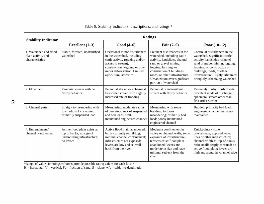
Table 8. Stability indicators, descriptions, and ratings.*

Ratings Stability Indicator

Excellent (1–3) Good (4–6) Fair (7–9) Poor (10–12)

1. Watershed and flood plain activity and characteristics

Stable, forested, undisturbed watershed

Occasional minor disturbances in the watershed, including cattle activity (grazing and/or access to stream), construction, logging, or other minor deforestation. Limited agricultural activities

Frequent disturbances in the watershed, including cattle activity, landslides, channel sand or gravel mining, logging, farming, or construction of buildings, roads, or other infrastructure. Urbanization over significant portion of watershed

Continual disturbances in the watershed. Significant cattle activity, landslides, channel sand or gravel mining, logging, farming, or construction of buildings, roads, or other infrastructure. Highly urbanized or rapidly urbanizing watershed

2. Flow habit Perennial stream with no flashy behavior

Perennial stream or ephemeral first-order stream with slightly increased rate of flooding

Perennial or intermittent stream with flashy behavior

Extremely flashy; flash floods prevalent mode of discharge; ephemeral stream other than first-order stream

3. Channel pattern Straight to meandering with low radius of curvature; primarily suspended load

Meandering, moderate radius of curvature; mix of suspended and bed loads; well-maintained engineered channel

Meandering with some braiding; tortuous meandering; primarily bed load; poorly maintained engineered channel

Braided; primarily bed load; engineered channel that is not maintained

4. Entrenchment/ channel confinement

Active flood plain exists at top of banks; no sign of undercutting infrastructure; no levees

Active flood plain abandoned, but is currently rebuilding; minimal channel confinement; infrastructure not exposed; levees are low and set well back from the river

Moderate confinement in valley or channel walls; some exposure of infrastructure; terraces exist; flood plain abandoned; levees are moderate in size and have minimal setback from the river

Knickpoints visible downstream; exposed water lines or other infrastructure; channel-width-to-top-of-banks ratio small; deeply confined; no active flood plain; levees are high and along the channel edge

*Range of values in ratings columns provide possible rating values for each factor H = horizontal, V = vertical, Fs = fraction of sand, S = slope, w/y = width-to-depth ratio

65

Table 8. Stability indicators, descriptions, and ratings, continued.

Ratings Stability Indicator

Excellent (1–3) Good (4–6) Fair (7–9) Poor (10–12)

5. Bed material Fs = approximate portion of sand in the bed

Assorted sizes tightly packed, overlapping, and possibly imbricated. Most material > 4 mm. Fs < 20%

Moderately packed with some overlapping. Very small amounts of material < 4 mm. 20 < Fs < 50%

Loose assortment with no apparent overlap. Small to medium amounts of material < 4 mm. 50 < Fs < 70%

Very loose assortment with no packing. Large amounts of material < 4 mm. Fs > 70%

6. Bar development

For S < 0.02 and w/y > 12, bars are mature, narrow relative to stream width at low flow, well vegetated, and composed of coarse gravel to cobbles. For S > 0.02 and w/y < 12, no bars are evident

For S < 0.02 and w/y > 12, bars may have vegetation and/or be composed of coarse gravel to cobbles, but minimal recent growth of bar evident by lack of vegetation on portions of the bar. For S > 0.02 and w/y < 12, no bars are evident

For S < 0.02 and w/y > 12, bar widths tend to be wide and composed of newly deposited coarse sand to small cobbles and/or may be sparsely vegetated. Bars forming for S > 0.02 and w/y < 12

Bar widths are generally greater than 1/2 the stream width at low flow. Bars are composed of extensive deposits of fine particles up to coarse gravel with little to no vegetation. No bars for S < 0.02 and w/y > 12

7. Obstructions, including bedrock outcrops, armor layer, LWD jams, grade control, bridge bed paving, revetments, dikes or vanes, riprap

Rare or not present Occasional, causing cross currents and minor bank and bottom erosion

Moderately frequent and occasionally unstable obstructions, cause noticeable erosion of the channel. Considerable sediment accumulation behind obstructions

Frequent and often unstable, causing a continual shift of sediment and flow. Traps are easily filled, causing channel to migrate and/or widen

8. Bank soil texture and coherence

Clay and silty clay; cohesive material

Clay loam to sandy clay loam; minor amounts of noncohesive or unconsolidated mixtures; layers may exist, but are cohesive materials

Sandy clay to sandy loam; unconsolidated mixtures of glacial or other materials; small layers and lenses of noncohesive or unconsolidated mixtures

Loamy sand to sand; noncohesive material; unconsolidated mixtures of glacial or other materials; layers or lenses that include noncohesive sands and gravels

H = horizontal, V = vertical, Fs = fraction of sand, S = slope, w/y = width-to-depth ratio

66

Table 8. Stability indicators, descriptions, and ratings, continued.

Ratings Stability Indicator

Excellent (1–3) Good (4–6) Fair (7–9) Poor (10–12)

9. Average bank slope angle (where 90E is a vertical bank)

Bank slopes < 3H:1V (18E) for noncohesive or unconsolidated materials to < 1:1 (45E) in clays on both sides

Bank slopes up to 2H:1V (27E) in noncohesive or unconsolidated materials to 0.8:1 (50E) in clays on one or occasionally both banks

Bank slopes to 1H:1V (45E) in noncohesive or unconsolidated materials to 0.6:1 (60E) in clays common on one or both banks

Bank slopes over 45E in noncohesive or unconsolidated materials or over (60E) in clays common on one or both banks

10. Vegetative or engineered bank protection

Wide band of woody vegetation with at least 90% density and cover. Primarily hard wood, leafy, deciduous trees with mature, healthy, and diverse vegetation located on the bank. Woody vegetation oriented vertically. In absence of vegetation, both banks are lined or heavily armored

Medium band of woody vegetation with 70–90% plant density and cover. A majority of hard wood, leafy, deciduous trees with maturing, diverse vegetation located on the blank. Woody vegetation oriented 80–90E from horizontal with minimal root exposure. Partial lining or armoring of one or both banks

Small band of woody vegetation with 50–70% plant density and cover. A majority of soft wood, piney, coniferous trees with young or old vegetation lacking in diversity located on or near the top of bank. Woody vegetation oriented at 70–80E from horizontal, often with evident root exposure. No lining of banks, but some armoring may be in place on one bank

Woody vegetation band may vary depending on age and health with less than 50% plant density and cover. Primarily soft wood, piney, coniferous trees with very young, old and dying, and/or monostand vegetation located off of the bank. Woody vegetation oriented at less than 70E from horizontal with extensive root exposure. No lining or armoring of banks

11. Bank cutting

Little or none evident. Infrequent raw banks, insignificant percentage of total bank

Some intermittently along channel bends and at prominent constrictions. Raw banks comprise minor portion of bank in vertical direction

Significant and frequent on both banks. Raw banks comprise large portion of bank in vertical direction. Root mat overhangs

Almost continuous cuts on both banks, some extending over most of the banks. Undercutting and sod-root overhangs

H = horizontal, V = vertical, Fs = fraction of sand, S = slope, w/y = width-to-depth ratio

67

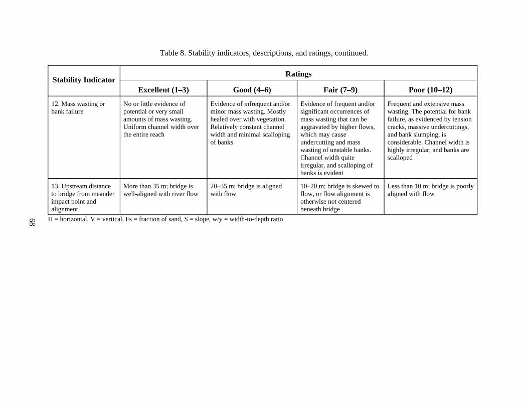
Table 8. Stability indicators, descriptions, and ratings, continued.

Ratings Stability Indicator

Excellent (1–3) Good (4–6) Fair (7–9) Poor (10–12)

12. Mass wasting or bank failure

No or little evidence of potential or very small amounts of mass wasting. Uniform channel width over the entire reach

Evidence of infrequent and/or minor mass wasting. Mostly healed over with vegetation. Relatively constant channel width and minimal scalloping of banks

Evidence of frequent and/or significant occurrences of mass wasting that can be aggravated by higher flows, which may cause undercutting and mass wasting of unstable banks. Channel width quite irregular, and scalloping of banks is evident

Frequent and extensive mass wasting. The potential for bank failure, as evidenced by tension cracks, massive undercuttings, and bank slumping, is considerable. Channel width is highly irregular, and banks are scalloped

13. Upstream distance to bridge from meander impact point and alignment

More than 35 m; bridge is well-aligned with river flow

20–35 m; bridge is aligned with flow

10–20 m; bridge is skewed to flow, or flow alignment is otherwise not centered beneath bridge

Less than 10 m; bridge is poorly aligned with flow

H = horizontal, V = vertical, Fs = fraction of sand, S = slope, w/y = width-to-depth ratio

68

Table 9. Stability assessment ratings for each factor.

Indicator Stream

1 2 3 4 5 6 7 8 9 10 11 12 13 Total Rating Based on

Tables 11–13

Saline R. 6 9 7 3 9 6 4 9 3 4 2 2 3 67 Good

SF Solomon R. 6 10 8 4 11 5 2 12 7 8 2 3 3 81 Good

N. Rush Cr. 5 9 6 7 9 2 2 9 6 10 5 5 9 84 Good

Arkansas R. 4 3 5 2 5 2 5 9 2 6 3 4 4 54 Good

Tomichi Cr. 7 3 5 2 9 3 4 7 5 5 3 2 7 62 Good

Murietta Cr. 12 12 9 7 11 5 2 11 9 10 8 7 3 106 Fair

Jacalitos Cr. 9 12 10 7 11 8 3 11 8 10 6 7 8 110 Fair

Dry Cr. 3 7 3 7 3 2 9 3 8 5 4 4 5 63 Good

Dutch Bill Cr. 2 8 5 7 7 10 5 8 8 3 6 4 10 83 Good

Buena Vista Cr. 8 11 10 7 12 10 2 11 10 11 10 10 4 116 Fair

Mojave R. 10 12 12 6 12 12 5 12 7 12 12 11 8 131 Poor

Rt. 66 Wash 10 12 10 6 8 10 9 11 10 12 12 11 11 132 Poor

Sacramento Wash 9 12 10 6 10 10 9 11 12 10 12 9 4 124 Fair

Rio San Jose 8 7 4 9 9 4 6 10 10 9 9 9 6 100 Fair

Rio Puerco 8 7 6 10 11 10 9 12 12 11 12 12 10 130 Poor

W. Elk Creek 7 4 5 8 10 6 9 7 11 8 9 10 3 97 Fair

Beaver Cr. 12 4 6 12 11 10 10 12 12 11 12 12 3 127 Poor

Brush Cr. 10 6 6 10 8 4 7 11 10 9 7 8 3 99 Fair

N 19 7 7 6 8 10 10 7 7 8 7 8 7 8 100 Fair R. = River, Cr. = Creek

69

Table 9. Stability assessment ratings for each factor, continued.

Indicator Stream

1 2 3 4 5 6 7 8 9 10 11 12 13 Total Rating Based on

Tables 11–13

Little Skin Cr. 6 5 6 5 5 6 9 7 9 9 6 10 8 91 Fair

N 21 6 7 3 6 9 4 8 8 10 7 5 3 10 86 Fair

Little Cypress Cr. 8 6 6 11 10 8 7 6 12 7 12 9 8 110 Fair

N 23 5 4 7 12 10 11 9 6 12 9 7 12 8 112 Fair

N 24 7 5 6 10 11 6 6 5 10 9 5 6 3 89 Fair

Honey Run 4 3 2 6 5 4 4 5 10 9 5 11 10 78 Good

South Fork 3 3 3 7 7 2 4 4 8 8 6 6 3 64 Good

East Fork 8 5 6 7 6 4 5 5 10 11 6 5 10 88 Fair

N 28 9 5 6 7 3 4 8 4 10 8 7 4 4 79 Good

McKnown Cr. 3 3 5 7 3 3 7 3 9 11 7 6 4 71 Good

Wolf Run 3 3 6 9 2 4 9 9 11 11 11 11 9 98 Fair

Alligator Cr. 8 2 4 5 3 5 5 8 5 2 2 2 6 57 Good

Peace R. 4 2 8 2 12 5 8 11 5 5 4 7 4 77 Good

Blackrock Run 7 4 5 8 7 7 5 7 10 8 4 7 5 84 Good

Indian Run 5 3 8 7 5 8 8 5 8 10 4 9 10 90 Fair

Middle Patuxent R. 5 2 5 4 3 3 4 5 9 5 8 7 7 67 Good

Hammond Branch 11 9 8 8 9 9 7 6 10 9 10 9 11 116 Fair

Atherton Tributary 5 6 5 6 6 5 4 5 8 8 6 6 4 74 Good

Stocketts Run 3 3 4 6 7 8 5 2 7 5 8 4 11 73 Good R. = River, Cr. = Creek

70

Table 9. Stability assessment ratings for each factor, continued.

Indicator Stream

1 2 3 4 5 6 7 8 9 10 11 12 13 Total Rating Based on

Tables 11–13

Mill Stream Branch 6 4 3 7 10 8 5 3 8 7 4 4 3 72 Good

Kent County Tributary 4 3 4 10 10 9 7 3 11 9 9 10 9 98 Fair

Morgan Cr. 8 5 5 4 9 5 4 3 9 9 10 6 11 88 Fair

Little Elk Cr. 5 2 3 2 2 3 3 4 5 3 4 2 8 46 Excellent

Big Beaver Cr. 11 5 5 4 10 12 6 5 10 12 12 10 10 112 Fair

Buffalo Run 7 4 6 5 5 4 5 2 9 11 9 7 4 78 Good

Roaring Run 2 2 2 2 2 5 3 3 4 3 3 1 8 40 Excellent

Potter Run 3 3 3 3 1 2 4 2 6 9 8 4 4 52 Good

Bentley Cr. 10 9 10 7 9 6 5 12 12 8 11 8 12 119 Fair

N 48 2 3 3 5 1 2 4 1 5 1 4 2 8 41 Excellent

Reids Run 3 3 3 5 1 4 4 3 6 5 4 2 7 50 Good

Piney Cr. 4 3 4 4 3 5 4 5 7 9 4 2 9 63 Good

L. Sandy Cr. 6 4 4 6 3 5 3 3 8 10 6 8 8 74 Good

Trout Run 4 3 3 3 4 3 3 3 6 1 2 1 7 43 Excellent

Pootatuck R. 4 3 3 4 1 2 4 3 5 5 5 4 8 51 Good

Mill R. 3 2 5 3 6 2 4 8 6 6 6 2 12 65 Good

Aspetuck R. 5 3 3 5 7 4 4 7 5 5 6 2 3 59 Good

W. Br. Saugatuck R. 6 3 7 3 5 2 11 6 3 3 6 1 8 64 Good

Mianus R. 3 2 3 3 4 3 3 4 5 4 4 1 5 44 Excellent R. = River, Cr. = Creek

71

72

Table 10. Overall rankings for pool-riffle, plane-bed, dune-ripple, and engineered channels.

Category Ranking, R

Excellent R < 49

Good 49 # R < 85

Fair 85 # R < 120

Poor 120 # R

Table 11. Overall rankings for cascade and step-pool channels.

Category Ranking, R

Excellent R < 41

Good 41 # R < 70

Fair 70 # R < 98

Poor 98 # R

Table 12. Overall rankings for braided channels.

Category Ranking, R

Excellent N/A

Good R < 94

Fair 94 # R < 129

Poor 129 # R

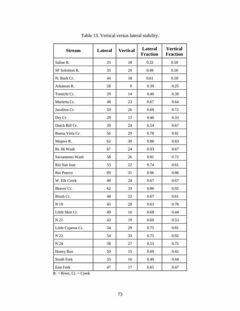
73

Table 13. Vertical versus lateral stability.

Stream Lateral Vertical Lateral Fraction

Vertical Fraction

Saline R. 23 18 0.32 0.50

SF Solomon R. 35 20 0.49 0.56

N. Rush Cr. 44 18 0.61 0.50

Arkansas R. 28 9 0.39 0.25

Tomichi Cr. 29 14 0.40 0.39

Murietta Cr. 48 23 0.67 0.64

Jacalitos Cr. 50 26 0.69 0.72

Dry Cr. 29 12 0.40 0.33

Dutch Bill Cr. 39 24 0.54 0.67

Buena Vista Cr. 56 29 0.78 0.81

Mojave R. 62 30 0.86 0.83

Rt. 66 Wash 67 24 0.93 0.67

Sacramento Wash 58 26 0.81 0.72

Rio San Jose 53 22 0.74 0.61

Rio Puerco 69 31 0.96 0.86

W. Elk Creek 48 24 0.67 0.67

Beaver Cr. 62 33 0.86 0.92

Brush Cr. 48 22 0.67 0.61

N 19 45 28 0.63 0.78

Little Skin Cr. 49 16 0.68 0.44

N 21 43 19 0.60 0.53

Little Cypress Cr. 54 29 0.75 0.81

N 23 54 33 0.75 0.92

N 24 38 27 0.53 0.75

Honey Run 50 15 0.69 0.42

South Fork 35 16 0.49 0.44

East Fork 47 17 0.65 0.47 R. = River, Cr. = Creek

74

Table 13. Vertical versus lateral stability, continued.

Stream Lateral Vertical Lateral Fraction

Vertical Fraction

N 28 37 14 0.51 0.39

McKnown Cr. 40 13 0.56 0.36

Wolf Run 62 15 0.86 0.42

Alligator Cr. 25 13 0.35 0.36

Peace R. 36 19 0.50 0.53

Blackrock Run 41 22 0.57 0.61

Indian Run 46 20 0.64 0.56

Middle Patuxent R. 41 10 0.57 0.28

Hammond Branch 55 26 0.76 0.72

Atherton Tributary 37 17 0.51 0.47

Stocketts Run 37 21 0.51 0.58

Mill Stream Branch 29 25 0.40 0.69

Kent Co. Tributary 51 29 0.71 0.81

Morgan Creek 48 18 0.67 0.50

Little Elk Cr. 26 7 0.36 0.19

Big Beaver Cr. 59 26 0.82 0.72

Buffalo Run 42 14 0.58 0.39

Roaring Run 22 9 0.31 0.25

Potter Run 33 6 0.46 0.17

Bentley Cr. 63 22 0.88 0.61

N 48 21 8 0.29 0.22

Reids Run 27 10 0.38 0.28

Piney Cr. 36 12 0.50 0.33

L. Sandy Cr. 43 14 0.60 0.39

Trout Run 20 10 0.28 0.28

Pootatuck R. 30 7 0.42 0.19

Mill R. 40 11 0.56 0.31 R. = River, Cr. = Creek

75

Table 13. Vertical versus lateral stability, continued.

Stream Lateral Vertical Lateral Fraction

Vertical Fraction

Aspetuck R. 28 16 0.39 0.44

W. Br. Saugatuck R. 27 10 0.38 0.28

Mianus R. 23 10 0.32 0.28 R. = River, Cr. = Creek

HEC-20 suggests that the lateral and vertical stability be examined as well as the overall stability. The indicators in table 8 can be divided into those that indicate vertical stability and those that indicate lateral stability. Results are given in table 13 in which vertical stability is described by indicators 4–6, while lateral stability is described by indicators 8–13. Each of the lateral and vertical stability ratings were normalized by the total number of points possible in each category so that they could be represented as a fraction and more readily compared. Thus, the lateral score was divided by 72 and the vertical score by 36. If the lateral score fraction is greater than the vertical score fraction, then it can be expected that the channel instability is primarily in the lateral direction. As an example, the Route 66 Wash is rated as “poor.” However, the lateral score fraction is significantly higher than the vertical score fraction (0.93 versus 0.67), indicating that lateral instability is dominant. If, on the other hand, the vertical score fraction is greater than the lateral, then bed degradation is the dominant source of instability. An example of this type of scores is given by Wolf Run, for which the vertical score fraction is about double the lateral score fraction, indicating primarily vertical instability. If both scores are high, then the channel is unstable due to both lateral and vertical processes. For example, Beaver Creek has lateral and vertical fractions of 0.86 and 0.92, respectively. This indicates that the channel is both degrading and widening. The processes may be ongoing simultaneously or they may be occurring differentially. This is frequently the case—as a knickpoint moves upstream, the channel banks respond by collapsing and widening, then another knickpoint moves through, and the process repeats. If both scores are low, this indicates minimal instability in either direction. For example, Alligator Creek has similar scores in both lateral and vertical categories, indicating healthy adjustments in both directions. Occasionally, rating each of the 13 factors for a particular bridge will result in one factor which stands out as being much higher (worse) than the others. For example, Little Elk Creek received an excellent as the overall rating. All of the assessment factors received scores between 2 and 5, except for the alignment factor (#13). This factor was given a rating of 8 due to the fact that the right abutment of the bridge was located just downstream of the outside of a gentle meander bend. The meander bend appears to be migrating at a very slow rate; this is based on observations that there is undercutting of tree roots on the right bank, but all trees are oriented vertically. Although the rate of lateral migration appears to be slow, it is worth noting and making additional observations during future inspections.

76

In collecting the data and observations for this method, the engineer or other inspector should walk some distance upstream and downstream from the bridge, rather than just observe from the bridge itself. The appropriate distance, however, depends on several factors, such as uniformity of stream conditions, magnitude of disturbances along the banks, in the flood plain, or in the watershed, time available, and accessibility. Ideally, the observer should walk at least 10 channel widths upstream and downstream of the bridge. Although it is possible to establish stability conditions in less distance, the more of the stream that is observed, the better understanding the observer will have of causes, processes, and rates of change. Bridges often divide property and sometimes divide geomorphic features or regions. Thus, conditions upstream and downstream of the bridge may be significantly different. In this case, it may be necessary to conduct separate analyses upstream and downstream. Unless the disturbance downstream of the bridge is traveling upstream, as in knickpoint migration or lateral migration of an adjacent meander, then the conditions downstream will be unlikely to affect the bridge, and more emphasis should be placed on the upstream conditions.

77

5. MODIFICATIONS OF THORNE’S RECONNAISSANCE SHEETS The stream stability assessment method developed in chapter 4 is self-contained and does not require any other data or formal method of data collection other than the descriptors given in table 8. However, it is prudent to develop field forms that help observers focus attention on specific aspects of a stream, be consistent in those observations, and systematically record their observations. For this purpose, the Thorne reconnaissance field sheets are the best method available for systematically collecting stream channel data. There are several problems with using the reconnaissance field sheets developed by Thorne for highway-related purposes.(2) First, it is not clear that this highly detailed and time-consuming level of data collection is necessary to assess stream stability or stream response at a bridge. In addition, bridge inspectors generally cannot and will not take the time to collect this level of data, as it is out of line with the overall inspection process. Second, even when all of the detailed data are collected, there is no guidance within the method for interpreting the data. Third, few inspectors and hydraulic engineers have appropriate backgrounds to identify geological parameters, such as rock type. To develop a rapid stability assessment method, a simplified version of the Thorne reconnaissance sheets should be created specifically for use in training and data collection associated with assessing stream stability at bridges. The stream stability method developed for this report is based on data collected through the reconnaissance. However, given that bridge inspection requires only assessment of stream stability in the short term and since each bridge is inspected at least every 2 years, data collection requirements can be simplified to reflect this less detailed and rapid assessment. In addition, several aspects of the sheets required minimal revision. Interpretive observations, while critical to communicating between observers, are neglected in the revised sheets because, in a rapid assessment, most of the qualitative data are collected by an inspector who is interpreting what he or she observes. All inspections require written reports in which the inspector provides his or her judgment on the status of the overall bridge condition and maintenance needs. In addition, items on the sheet that cannot be assessed in a very brief site visit are excluded from the revised sheets. The simplified and revised data collection sheets, based strongly on Thorne’s reconnaissance sheets, are given in figures 18–20. In addition to the stability assessment, keeping a record of channel dimensions upstream and downstream of the bridge will provide a history of changes in width and depth. Although detailed surveys are not part of a bridge inspection, a simple measurement of station and elevation upstream of the bridge taken annually will provide adequate cross-sectional information to assess longer term changes. Without this information, gradual but continual changes in the channel may be overlooked.

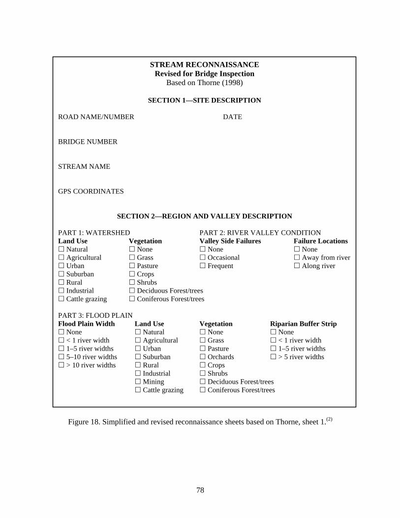
78

Figure 18. Simplified and revised reconnaissance sheets based on Thorne, sheet 1.(2)

STREAM RECONNAISSANCE Revised for Bridge Inspection

Based on Thorne (1998)

SECTION 1—SITE DESCRIPTION ROAD NAME/NUMBER DATE BRIDGE NUMBER STREAM NAME GPS COORDINATES

SECTION 2—REGION AND VALLEY DESCRIPTION PART 1: WATERSHED PART 2: RIVER VALLEY CONDITION Land Use Vegetation Valley Side Failures Failure Locations

Natural None None None Agricultural Grass Occasional Away from river Urban Pasture Frequent Along river Suburban Crops Rural Shrubs Industrial Deciduous Forest/trees Cattle grazing Coniferous Forest/trees

PART 3: FLOOD PLAIN Flood Plain Width Land Use Vegetation Riparian Buffer Strip

None Natural None None < 1 river width Agricultural Grass < 1 river width 1–5 river widths Urban Pasture 1–5 river widths 5–10 river widths Suburban Orchards > 5 river widths > 10 river widths Rural Crops

Industrial Shrubs Mining Deciduous Forest/trees Cattle grazing Coniferous Forest/trees

79

Figure 19. Simplified and revised reconnaissance sheets based on Thorne, sheet 2.(2)

PART 4: VERTICAL CONFINEMENT Terraces Levees Levee Location

None None Along channel bank Left bank Natural Setback < 1 river width Right bank Constructed Setback > 1 river width

PART 5: LATERAL RELATION OF CHANNEL TO VALLEY Planform Meander Characteristics

Straight Mild bends Meandering Moderate bends Braided Tight bends Anastomosed Engineered

SECTION 3—CHANNEL DESCRIPTION

PART 6: CHANNEL DESCRIPTION (select all that apply) Bed Controls Control Types Width Controls Control Types Other

None None None None Debris Occasional Bedrock Occasional Bedrock Mining Frequent Boulders Frequent Boulders Reservoir Confined Gravel armor Confined Gravel armor Knickpoint

Bridge protection Bridge protection Grade control Bridge abutments Debris Bank stabilization Dams (beaver, engineered) Debris Flow Habit Channel Width = ___________

Perennial Flashy perennial M-B Classification Corps Classification (Other) Intermittent Cascade or step-pool Modified (engineered) Ephemeral Plane, pool-riffle, dune-ripple Regulated

Braided Arroyo PART 7: BED SEDIMENT DESCRIPTION (select all that apply) Bed Material Bar Types Bar Material Bar Vegetation Bar Width

Clay None Silt None None Silt Alternate bars Sand Grasses Narrow Sand Point bars Gravel Reeds/shrubs Moderate Gravel Midchannel bars Cobbles Trees Wide Cobbles Diagonal bars Boulders Irregular/combination Bedrock Braided Percent Sand in Bed = ____________%

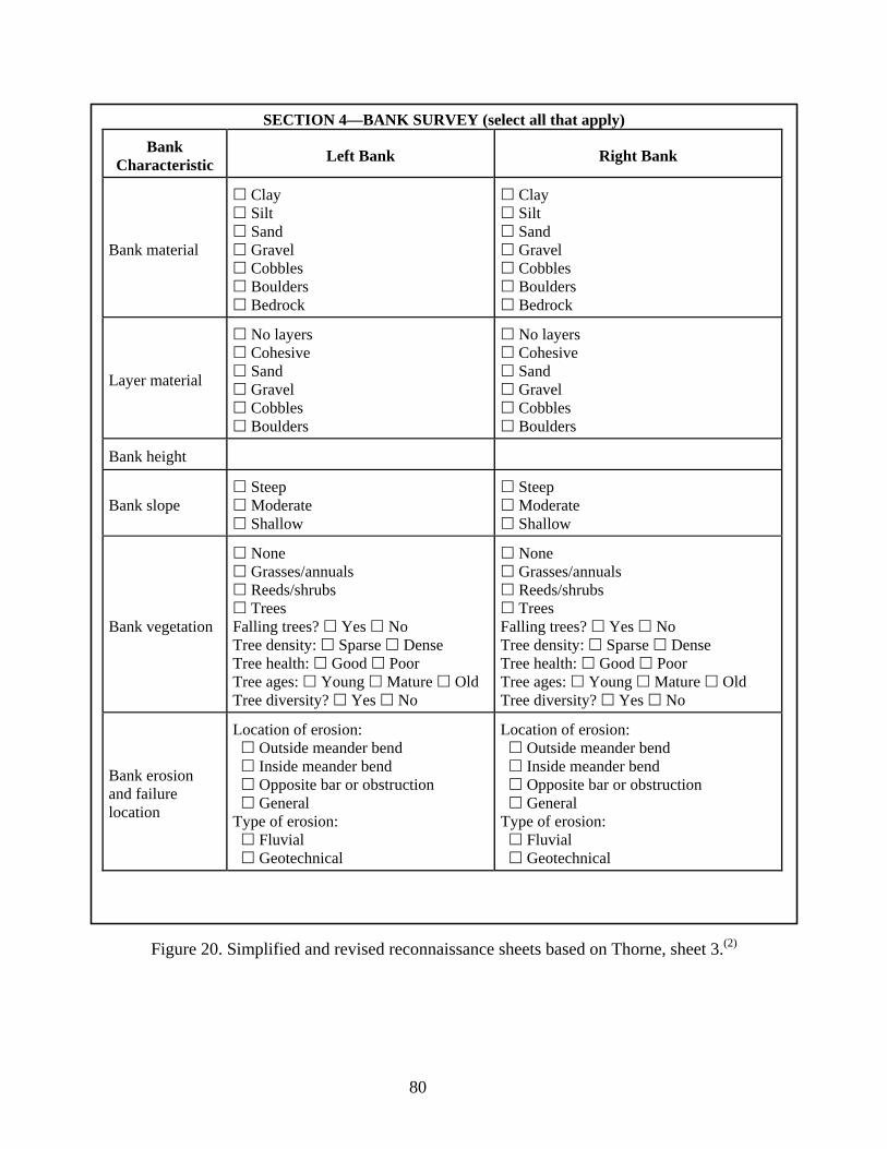
80

Figure 20. Simplified and revised reconnaissance sheets based on Thorne, sheet 3.(2)

SECTION 4—BANK SURVEY (select all that apply)

Bank Characteristic Left Bank Right Bank

Bank material

Clay Silt Sand Gravel Cobbles Boulders Bedrock

Clay Silt Sand Gravel Cobbles Boulders Bedrock

Layer material

No layers Cohesive Sand Gravel Cobbles Boulders

No layers Cohesive Sand Gravel Cobbles Boulders

Bank height

Bank slope Steep Moderate Shallow

Steep Moderate Shallow

Bank vegetation

None Grasses/annuals Reeds/shrubs Trees

Falling trees? Yes No Tree density: Sparse Dense Tree health: Good Poor Tree ages: Young Mature Old Tree diversity? Yes No

None Grasses/annuals Reeds/shrubs Trees

Falling trees? Yes No Tree density: Sparse Dense Tree health: Good Poor Tree ages: Young Mature Old Tree diversity? Yes No

Bank erosion and failure location

Location of erosion: Outside meander bend Inside meander bend Opposite bar or obstruction General Type of erosion: Fluvial Geotechnical

Location of erosion: Outside meander bend Inside meander bend Opposite bar or obstruction General Type of erosion: Fluvial Geotechnical

81

6. EXAMPLES This chapter provides two examples for using the stream stability assessment method based on photos shown in the appendix A. The first example is Jayne Avenue over Jacalitos Creek near Coalinga, CA. Using http://terraserver-usa.com and the coordinates in table 5, a larger view of the bridge-stream intersection can be seen. The stream is seen to be mobile laterally, as evidenced by the large scars, deposits, and remnant channels. The photos of Jacalitos Creek in appendix A show views of the channel upstream and downstream of the bridge. Using the modified Thorne reconnaissance sheets given in figures 18–20, data collection begins by recording the map location, the GPS location, and the date. Next, characteristics of the watershed and flood plain are recorded. From the aerial photo on http://terraserver-usa.com, it is clear that the watershed use is primarily agricultural, while at least a portion of the flood plain is natural to allow for lateral movement of the stream. A visit to the site showed that cattle grazing is also a large part of the land use. The channel is braided to meandering with a riparian buffer of trees and shrubs upstream, but minimal buffer downstream. The channel was classified according to the Montgomery-Buffington and USACE methods. This yields a dune-ripple bed that is meandering to braided. The width and depth measurements are taken upstream and downstream of the bridge at approximate bankfull elevation. (Note that these measurements are not needed for the assessment method, but provide a record from which to compare the channel over many years.) The number of measurements needed depends on the variability of the channel dimensions. For this channel, three measurements upstream and downstream of the bridge were adequate to describe an average width-to-depth ratio. The measurements should be taken out of the influence of the bridge so that contraction scour does not influence the recorded dimensions. The general rule of thumb for reach length is 20 channel widths. In this case, where the channel is fairly uniform, 10 widths upstream and 10 downstream are adequate. The remaining data are recorded for the channel sediment, obstructions, and bank characteristics. The primary purpose of recording these data on the modified Thorne sheets is to help familiarize the user with the channel, focus the user’s attention on various aspects of the channel, and provide a record of conditions that can be compared in subsequent years. While still onsite and after the reconnaissance sheets are filled out, the stability assessment sheet in table 8 should be used to determine the ratings for each of the 13 indicators. For Jacalitos Creek, the ratings and the total sum are given in table 9. Since this channel is in the dune-ripple category, table 10 is used to determine the overall rating. The second example is S.R. 445 over Roaring Run in the Valley and Ridge Province of central Pennsylvania. Photos for this channel are provided in appendix A. Using http://terraserver-usa.com and the coordinates in table 5 to obtain aerial photos provides a larger view of the channel, the bridge-channel intersection, and watershed characteristics. Land use is primarily natural forest. The channel classifies as a step-pool channel according to the Montgomery-Buffington method and a mountain torrent, according to the USACE method. The modified Thorne sheets are completed to familiarize and focus the user on the channel, flood plain, and watershed. In this channel, the dimensions and other characteristics are relatively constant, so 10 channel widths upstream and downstream were adequate for estimating average dimensions and other observations. Cross-sectional width and depth were measured at the approximate bankfull elevation. Since the channel is very uniform both upstream and downstream, only one to two cross sections needed to be measured. The detail of the cross-sectional measurement depends on

82

the user and the need to have detailed cross sections to compare in the future. For the purposes of the assessment method developed here, no cross-sectional data are used; however, as stated previously, it may be desirable to measure several cross sections in greater detail for future use. For the Thorne reconnaissance method, only an average width and depth are recorded. Although it is unnecessary for an initial or near-bridge channel stability assessment, it should be noted that walking much longer lengths of the channel can reveal disturbances that could eventually affect the bridge-channel intersection of interest. After the modified Thorne sheets are completed and the user is familiar with the stream, the stability assessment ratings can be determined. In this example, all indicators except for #13 show that the channel is very stable. The alignment of the channel and the bridge, however, cause #13 to be much higher than the others. The tight bend on which the bridge sits could clearly migrate in the future and cause problems at the bridge. Otherwise, the channel stability is rated as excellent, according to table 11. If a stability rating is determined to be fair or poor, it might be desirable to return to the site for more detailed channel measurements by survey. Lateral movement and bed degradation can be measured over time by using such detailed, repeated measurements. However, to conduct rapid, preliminary assessments, as provided in this report, such detailed measurements are not necessary. If a channel is deemed to be stable (good to excellent), additional detailed measurements likely will not be needed. Thus, this method can be used as a decisionmaking tool regarding the need for more detailed and costly assessments.

83

7. CONCLUSIONS The stream stability assessment method developed here provides a self-contained, preliminary assessment of channel stability conditions as they affect bridge foundations. This method provides a quick assessment of conditions for the purpose of judging whether a more extensive geomorphic study or complete hydraulics (HEC-20, Level II) and sediment transport analyses (HEC-20, Level III) are needed to assess further the potential for adverse conditions developing at the bridge. As such, the method assists in decisionmaking with respect to bridge design, repair, rehabilitation, or replacement. Although the stability assessment method was developed for use in any physiographic region in the United States, it was not possible to make observations within every region. In addition, it was not possible to sample every stream type and stream order within each region. Therefore, the method should be used cautiously and with questioning so that the results represent the stability at the bridge-stream intersection. The results of this project provide a simplified methodology for assessing channel stability at bridge-stream intersections. It is intended to be used by qualified bridge inspectors and hydraulic engineers. This method developed is self-contained and does not require any other data or formal method of data collection other than the descriptors given in table 8. However, field forms were developed based on Thorne to help observers focus attention on specific aspects of a stream, make consistent observations, and record the observations systematically.(2) A photo album of the bridges in this study is provided in appendix A.

85

APPENDIX A This section contains a photo album for bridge-stream intersections according to physiographic regions.

86

Figure 21. Dry Creek, Pacific Coastal— upstream from bridge.

Figure 22. Dry Creek, Pacific Coastal— downstream from bridge.

Figure 23. Dry Creek, Pacific Coastal— upstream under bridge, photo 1.

Figure 24. Dry Creek, Pacific Coastal— upstream under bridge, photo 2.

87

Figure 25. Dutch Bill Creek, Pacific Coastal— upstream from under bridge.

Figure 26. Dutch Bill Creek, Pacific Coastal—downstream at bridge.

Figure 27. Dutch Bill Creek, Pacific Coastal— downstream from under bridge.

Figure 28. Dutch Bill Creek, Pacific Coastal— upstream through bridge.

88

Figure 29. Buena Vista Creek, Pacific Coastal— upstream from bridge.

Figure 30. Buena Vista Creek, Pacific Coastal— downstream from bridge.

Figure 31. Buena Vista Creek, Pacific Coastal— downstream under bridge.

Figure 32. Buena Vista Creek, Pacific Coastal— upstream from under bridge.

89

Figure 33. Jacalitos Creek, Pacific Coastal— downstream from bridge.

Figure 34. Jacalitos Creek, Pacific Coastal— upstream from bridge.

Figure 35. Jacalitos Creek, Pacific Coastal— looking downstream at bridge.

Figure 36. Jacalitos Creek, Pacific Coastal— downstream from under bridge.

90

Figure 37. Murietta Creek, Pacific Coastal— downstream from bridge.

Figure 38. Murietta Creek, Pacific Coastal— upstream from bridge.

Figure 39. Murietta Creek, Pacific Coastal— upstream toward bridge.

Figure 40. Murietta Creek, Pacific Coastal— looking upstream at bridge.

91

Figure 41. Mojave River, Basin and Range— upstream from bridge, photo 1.

Figure 42. Mojave River, Basin and Range— upstream from bridge, photo 2.

Figure 43. Mojave River, Basin and Range— looking downstream at bridge.

Figure 44. Mojave River, Basin and Range— downstream from bridge.

92

Figure 45. Rt. 66 Wash, Basin and Range— upstream from bridge.

Figure 46. Rt. 66 Wash, Basin and Range— downstream from bridge.

Figure 47. Rt. 66 Wash, Basin and Range— looking downstream at bridge.

Figure 48. Rt. 66 Wash, Basin and Range— looking upstream at bridge.

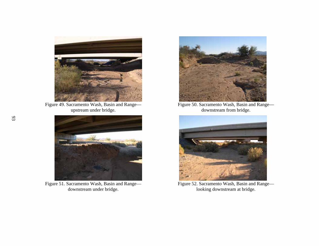
93

Figure 49. Sacramento Wash, Basin and Range— upstream under bridge.

Figure 50. Sacramento Wash, Basin and Range— downstream from bridge.

Figure 51. Sacramento Wash, Basin and Range— downstream under bridge.

Figure 52. Sacramento Wash, Basin and Range— looking downstream at bridge.

94

Figure 53. Rio Puerco, Trans Pecos— downstream from bridge.

Figure 54. Rio Puerco, Trans Pecos— upstream from bridge.

Figure 55. Rio Puerco, Trans Pecos— looking upstream at bridge.

Figure 56. Rio Puerco, Trans Pecos— looking downstream at bridge.

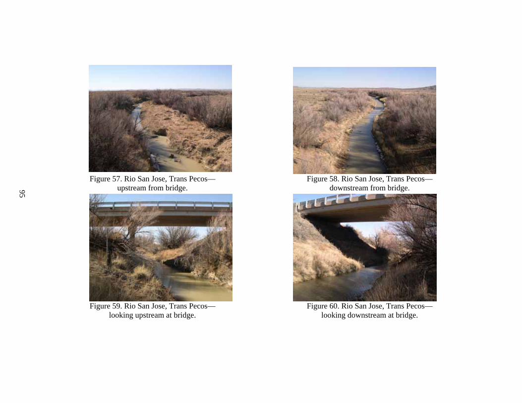
95

Figure 57. Rio San Jose, Trans Pecos— upstream from bridge.

Figure 58. Rio San Jose, Trans Pecos— downstream from bridge.

Figure 59. Rio San Jose, Trans Pecos— looking upstream at bridge.

Figure 60. Rio San Jose, Trans Pecos— looking downstream at bridge.

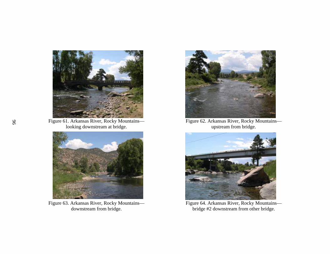
96

Figure 61. Arkansas River, Rocky Mountains— looking downstream at bridge.

Figure 62. Arkansas River, Rocky Mountains— upstream from bridge.

Figure 63. Arkansas River, Rocky Mountains— downstream from bridge.

Figure 64. Arkansas River, Rocky Mountains— bridge #2 downstream from other bridge.

97

Figure 65. Cochetopa Creek, Rocky Mountains— downstream from bridge.

Figure 66. Cochetopa Creek, Rocky Mountains— looking downstream at bridge.

Figure 67. Cochetopa Creek, Rocky Mountains— upstream from bridge.

98

Figure 68. North Rush Creek, Great Plains—upstream of bridge.

Figure 69. North Rush Creek, Great Plains— upstream from bridge.

Figure 70. North Rush Creek, Great Plains— downstream from bridge.

99

Figure 72. Saline River, Great Plains— downstream from bridge.

Figure 71. Saline River, Great Plains—upstream under bridge. Figure 73. Saline River, Great Plains— looking downstream at bridge.

100

Figure 74. South Fork Solomon River, Great Plains— looking downstream at bridge, photo 1.

Figure 75. South Fork Solomon River, Great Plains— looking downstream at bridge, photo 2.

Figure 76. South Fork Solomon River, Great Plains— left bank.

Figure 77. South Fork Solomon River, Great Plains—downstream.

101

Figure 78. West Elk Creek, Central Plains— looking downstream at bridge, photo 1.

Figure 79. West Elk Creek, Central Plains— looking downstream at bridge, photo 2.

Figure 80. West Elk Creek, Central Plains— upstream from bridge.

Figure 81. West Elk Creek, Central Plains— downstream from bridge.

102

Figure 82. Beaver Creek, Central Plains— upstream from bridge.

Figure 83. Beaver Creek, Central Plains— downstream from bridge.

Figure 84. Beaver Creek, Central Plains— facing upstream under bridge.

Figure 85. Beaver Creek, Central Plains— facing downstream under bridge.

103

Figure 87. Brush Creek, Central Plains— downstream from bridge.

Figure 86. Brush Creek, Central Plains—upstream from bridge. Figure 88. Brush Creek, Central Plains— downstream under bridge.

104

Figure 89. Unnamed creek (N 19), Central Plains— downstream from bridge.

Figure 90. Unnamed creek (N 19), Central Plains— upstream from bridge.

Figure 91. Unnamed creek (N 19), Central Plains— upstream under bridge.

Figure 92. Unnamed creek (N 19), Central Plains— downstream under bridge.

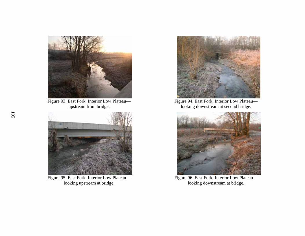
105

Figure 93. East Fork, Interior Low Plateau— upstream from bridge.

Figure 94. East Fork, Interior Low Plateau— looking downstream at second bridge.

Figure 95. East Fork, Interior Low Plateau— looking upstream at bridge.

Figure 96. East Fork, Interior Low Plateau— looking downstream at bridge.

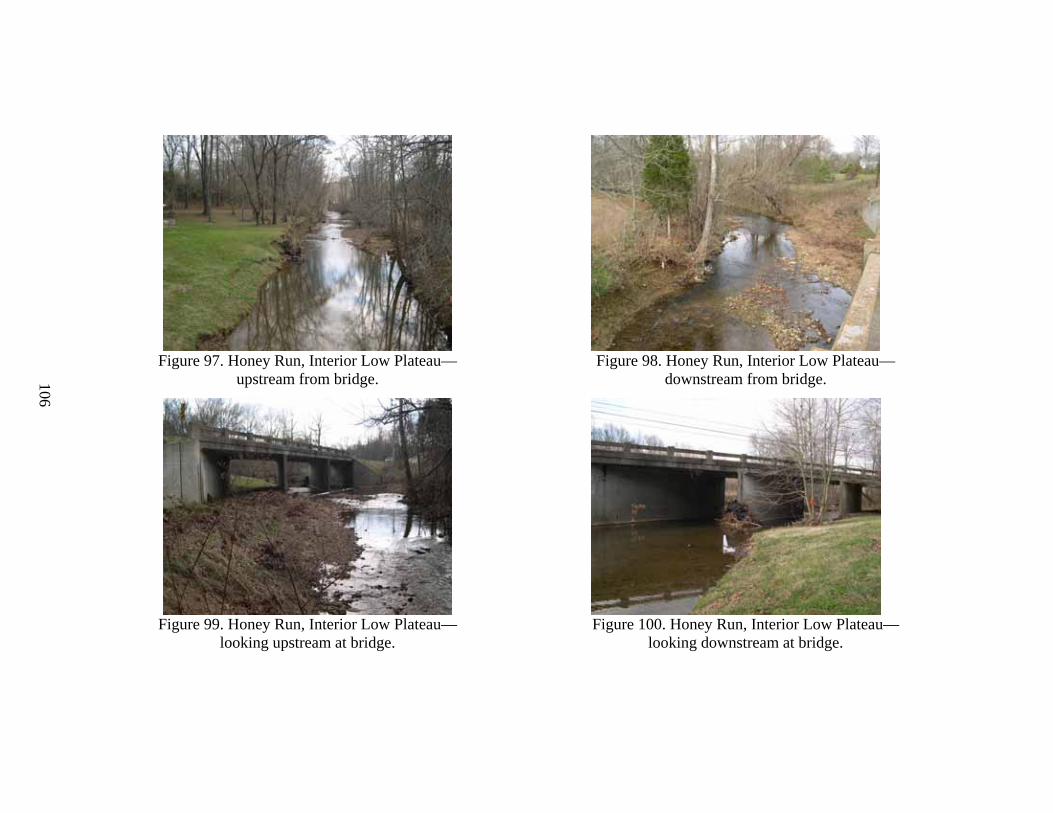
106

Figure 97. Honey Run, Interior Low Plateau— upstream from bridge.

Figure 98. Honey Run, Interior Low Plateau— downstream from bridge.

Figure 99. Honey Run, Interior Low Plateau— looking upstream at bridge.

Figure 100. Honey Run, Interior Low Plateau— looking downstream at bridge.

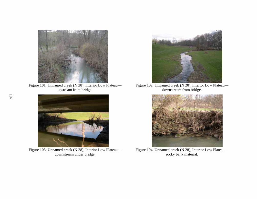
107

Figure 101. Unnamed creek (N 28), Interior Low Plateau—upstream from bridge.

Figure 102. Unnamed creek (N 28), Interior Low Plateau—downstream from bridge.

Figure 103. Unnamed creek (N 28), Interior Low Plateau—downstream under bridge.

Figure 104. Unnamed creek (N 28), Interior Low Plateau— rocky bank material.

108

Figure 105. South Fork, Interior Low Plateau— downstream from bridge.

Figure 106. South Fork, Interior Low Plateau— upstream from bridge.

Figure 107. South Fork, Interior Low Plateau— looking upstream at bridge.

Figure 108. South Fork, Interior Low Plateau— looking downstream at bridge.

109

Figure 109. Little Skin Creek, Ozark-Ouachita Highlands—downstream from bridge.

Figure 110. Little Skin Creek, Ozark-Ouachita Highlands—upstream from bridge.

Figure 111. Little Skin Creek, Ozark-Ouachita Highlands—looking downstream at bridge (left).

Figure 112. Little Skin Creek, Ozark-Ouachita Highlands—looking downstream at bridge (right).

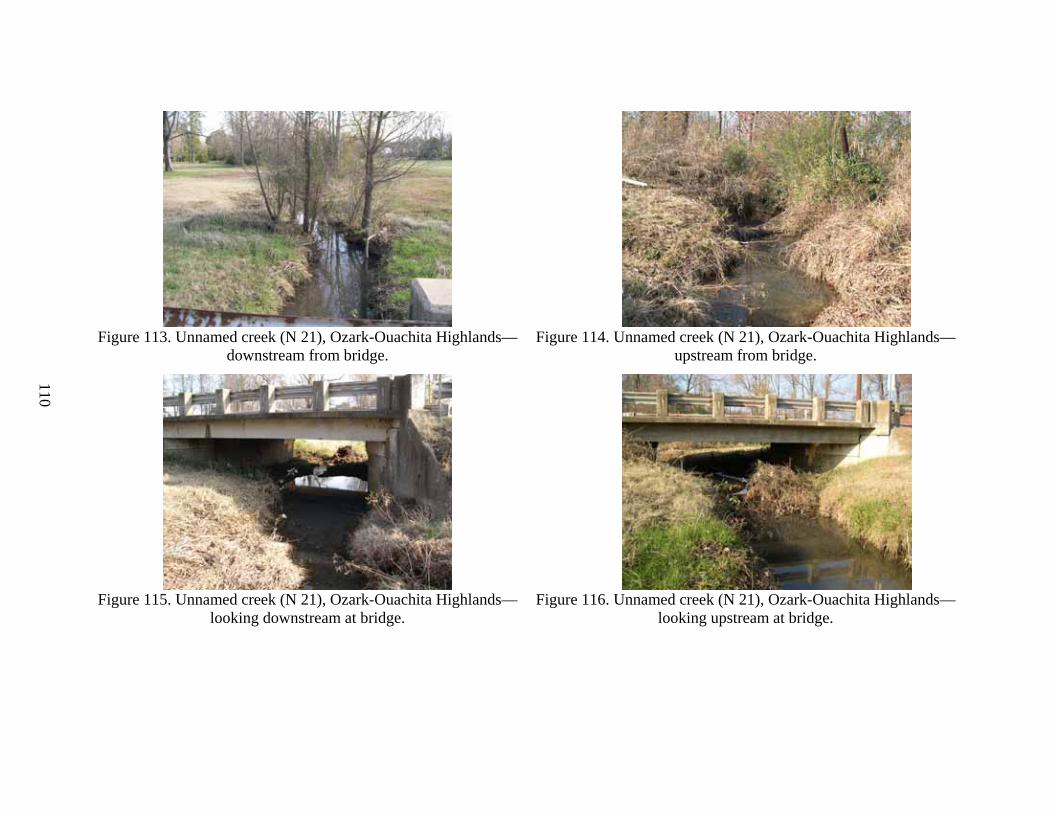
110

Figure 113. Unnamed creek (N 21), Ozark-Ouachita Highlands—downstream from bridge.

Figure 114. Unnamed creek (N 21), Ozark-Ouachita Highlands—upstream from bridge.

Figure 115. Unnamed creek (N 21), Ozark-Ouachita Highlands—looking downstream at bridge.

Figure 116. Unnamed creek (N 21), Ozark-Ouachita Highlands—looking upstream at bridge.

111

Figure 117. Little Cypress Creek, Atlantic Coastal Plain—downstream from bridge.

Figure 118. Little Cypress Creek, Atlantic Coastal Plain—upstream from bridge.

Figure 119. Little Cypress Creek, Atlantic Coastal Plain— looking downstream at bridge.

Figure 120. Little Cypress Creek, Atlantic Coastal Plain— looking upstream at bridge.

112

Figure 121. Unnamed creek (N 23), Atlantic Coastal Plain—downstream from bridge.

Figure 122. Unnamed creek (N 23), Atlantic Coastal Plain—upstream from bridge.

Figure 123. Unnamed creek (N 23), Atlantic Coastal Plain—looking downstream at bridge.

Figure 124. Unnamed creek (N 23), Atlantic Coastal Plain—looking upstream at bridge.

113

Figure 125. Unnamed creek (N 24), Atlantic Coastal Plain—upstream from bridge.

Figure 126. Unnamed creek (N 24), Atlantic Coastal Plain—downstream from bridge.

Figure 127. Unnamed creek (N 24), Atlantic Coastal Plain—looking upstream at bridge.

Figure 128. Unnamed creek (N 24), Atlantic Coastal Plain—looking downstream at bridge.

114

Figure 129. Peace River, Atlantic Coastal Plain— upstream from bridge at old pedestrian bridge.

Figure 130. Peace River, Atlantic Coastal Plain— looking downstream at bridge.

Figure 131. Peace River, Atlantic Coastal Plain— downstream under bridge, right bank.

Figure 132. Peace River, Atlantic Coastal Plain— upstream from old pedestrian bridge.

115

Figure 133. Alligator Creek, Atlantic Coastal Plain— downstream from bridge.

Figure 134. Alligator Creek, Atlantic Coastal Plain— looking downstream at bridge.

Figure 135. Alligator Creek, Atlantic Coastal Plain— looking upstream at bridge.

Figure 136. Alligator Creek, Atlantic Coastal Plain— upstream from bridge.

116

Figure 137. Stocketts Run, Atlantic Coastal Plain— upstream from bridge.

Figure 138. Stocketts Run, Atlantic Coastal Plain— downstream from bridge.

Figure 139. Stocketts Run, Atlantic Coastal Plain— looking downstream at bridge.

Figure 140. Stocketts Run, Atlantic Coastal Plain— looking upstream at bridge.

117

Figure 141. Mill Stream Branch, Atlantic Coastal Plain—upstream from bridge.

Figure 142. Mill Stream Branch, Atlantic Coastal Plain—downstream from bridge.

Figure 143. Mill Stream Branch, Atlantic Coastal Plain— looking downstream at bridge.

Figure 144. Mill Stream Branch, Atlantic Coastal Plain— looking upstream at bridge.

118

Figure 145. Kent County Tributary, Atlantic Coastal Plain—downstream from bridge.

Figure 146. Kent County Tributary, Atlantic Coastal Plain—upstream from bridge.

Figure 147. Kent County Tributary, Atlantic Coastal Plain—looking downstream at bridge.

Figure 148. Kent County Tributary, Atlantic Coastal Plain—looking upstream at bridge.

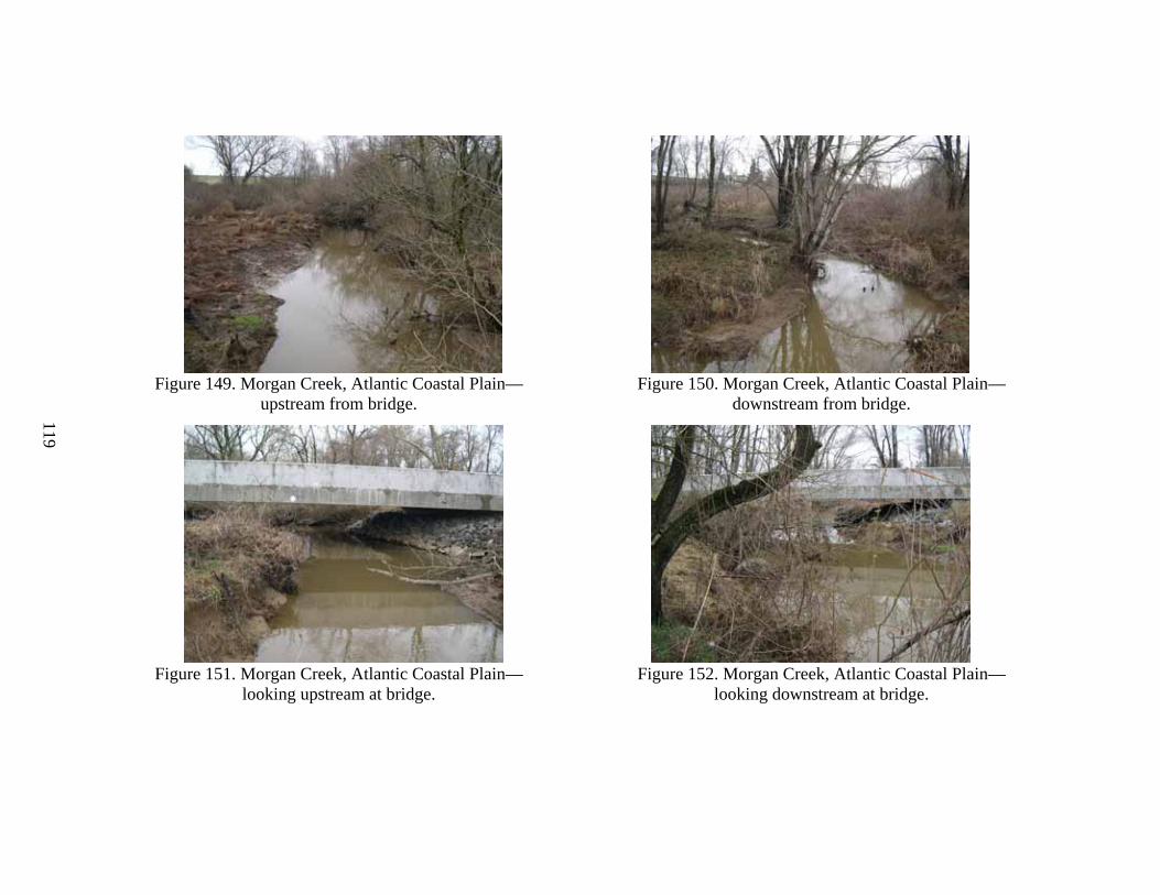
119

Figure 149. Morgan Creek, Atlantic Coastal Plain— upstream from bridge.

Figure 150. Morgan Creek, Atlantic Coastal Plain— downstream from bridge.

Figure 151. Morgan Creek, Atlantic Coastal Plain— looking upstream at bridge.

Figure 152. Morgan Creek, Atlantic Coastal Plain— looking downstream at bridge.

120

Figure 153. Hammond Branch, Atlantic Coastal Plain— upstream from bridge.

Figure 154. Hammond Branch, Atlantic Coastal Plain—downstream from bridge.

Figure 155. Hammond Branch, Atlantic Coastal Plain— looking downstream at bridge.

Figure 156. Hammond Branch, Atlantic Coastal Plain— looking upstream at bridge.

121

Figure 157. Pootatuck River, New England— downstream from bridge.

Figure 158. Pootatuck River, New England— upstream from bridge.

Figure 159. Pootatuck River, New England— looking downstream at bridge.

Figure 160. Pootatuck River, New England— looking upstream at bridge.

122

Figure 161. Mill River, New England— upstream from bridge.

Figure 162. Mill River, New England— downstream from bridge.

Figure 163. Mill River, New England— looking upstream at bridge.

Figure 164. Mill River, New England— looking downstream at bridge.

123

Figure 165. Aspetuck River, New England— upstream from bridge.

Figure 166. Aspetuck River, New England— downstream from bridge.

Figure 167. Aspetuck River, New England— looking upstream at bridge.

Figure 168. Aspetuck River, New England— looking downstream at bridge.

124

Figure 169. West Branch Saugatuck River, New England—downstream from bridge.

Figure 170. West Branch Saugatuck River, New England—upstream from bridge.

Figure 171. West Branch Saugatuck River, New England—looking downstream at bridge (bridge in foreground

is the pedestrian bridge).

Figure 172. West Branch Saugatuck River, New England—looking upstream at bridge.

125

Figure 173. Mianus River, New England— upstream from bridge.

Figure 174. Mianus River, New England— downstream from bridge. Note weir.

Figure 175. Mianus River, New England— looking downstream at bridge.

Figure 176. Mianus River, New England— looking upstream at bridge.

126

Figure 177. McKnown Creek, Appalachian Plateau— upstream from bridge.

Figure 178. McKnown Creek, Appalachian Plateau— downstream from bridge.

Figure 179. McKnown Creek, Appalachian Plateau— looking downstream at bridge.

Figure 180. McKnown Creek, Appalachian Plateau— looking upstream at bridge.

127

Figure 181. Wolf Run, Appalachian Plateau— upstream from bridge.

Figure 182. Wolf Run, Appalachian Plateau— downstream from bridge.

Figure 183. Wolf Run, Appalachian Plateau— looking upstream at bridge.

Figure 184. Wolf Run, Appalachian Plateau— upstream face of bridge.

128

Figure 185. Unnamed creek (N 48), Appalachian Plateau—upstream from bridge.

Figure 186. Unnamed creek (N 48), Appalachian Plateau—downstream from bridge.

Figure 187. Unnamed creek (N 48), Appalachian Plateau—looking downstream at bridge.

Figure 188. Unnamed creek (N 48), Appalachian Plateau—looking upstream through bridge.

129

Figure 189. Reids Run, Appalachian Plateau— upstream from bridge.

Figure 190. Reids Run, Appalachian Plateau— downstream from bridge.

Figure 191. Reids Run, Appalachian Plateau— looking downstream at bridge.

Figure 192. Reids Run, Appalachian Plateau— looking upstream at bridge.

130

Figure 193. Piney Creek, Appalachian Plateau— downstream from bridge.

Figure 194. Piney Creek, Appalachian Plateau— upstream from bridge.

Figure 195. Piney Creek, Appalachian Plateau— looking downstream at bridge.

Figure 196. Piney Creek, Appalachian Plateau— looking upstream at bridge.

131

Figure 197. Sandy Creek, Appalachian Plateau— upstream from bridge.

Figure 198. Sandy Creek, Appalachian Plateau— downstream from bridge.

Figure 199. Sandy Creek, Appalachian Plateau— looking downstream at bridge.

Figure 200. Sandy Creek, Appalachian Plateau— looking upstream at bridge.

132

Figure 201. Trout Run, Appalachian Plateau— upstream from bridge.

Figure 202. Trout Run, Appalachian Plateau— downstream from bridge.

Figure 203. Trout Run, Appalachian Plateau— looking upstream at bridge.

Figure 204. Trout Run, Appalachian Plateau— upstream face of bridge.

133

Figure 205. Blackrock Run, Piedmont— upstream from bridge.

Figure 206. Blackrock Run, Piedmont— downstream from bridge.

Figure 207. Blackrock Run, Piedmont— looking downstream at bridge.

Figure 208. Blackrock Run, Piedmont— looking upstream at bridge.

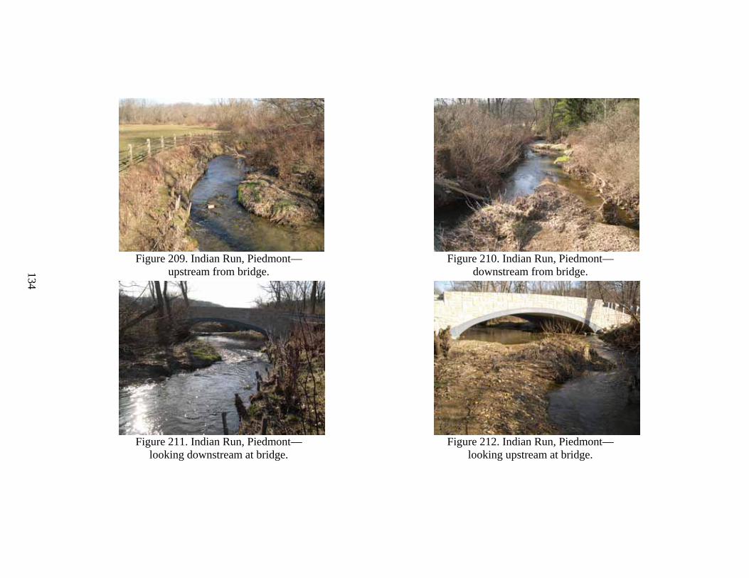
134

Figure 209. Indian Run, Piedmont— upstream from bridge.

Figure 210. Indian Run, Piedmont— downstream from bridge.

Figure 211. Indian Run, Piedmont— looking downstream at bridge.

Figure 212. Indian Run, Piedmont— looking upstream at bridge.

135

Figure 213. Middle Patuxent River, Piedmont— upstream from bridge.

Figure 214. Middle Patuxent River, Piedmont— downstream from bridge.

Figure 215. Middle Patuxent River, Piedmont— looking downstream at bridge.

Figure 216. Middle Patuxent River, Piedmont— looking upstream at bridge.

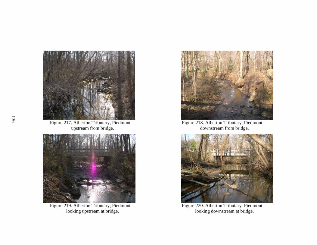
136

Figure 217. Atherton Tributary, Piedmont— upstream from bridge.

Figure 218. Atherton Tributary, Piedmont— downstream from bridge.

Figure 219. Atherton Tributary, Piedmont— looking upstream at bridge.

Figure 220. Atherton Tributary, Piedmont— looking downstream at bridge.

137

Figure 221. Little Elk Creek, Piedmont— upstream from bridge.

Figure 222. Little Elk Creek, Piedmont— downstream from bridge.

Figure 223. Little Elk Creek, Piedmont— looking upstream at bridge.

Figure 224. Little Elk Creek, Piedmont— looking downstream at bridge.

138

Figure 225. Big Beaver Creek, Piedmont— upstream from bridge.

Figure 226. Big Beaver Creek, Piedmont— downstream from bridge.

Figure 227. Big Beaver Creek, Piedmont— looking downstream at bridge.

Figure 228. Big Beaver Creek, Piedmont— looking upstream at bridge.

139

Figure 229. Buffalo Run, Valley and Ridge— upstream from bridge.

Figure 230. Buffalo Run, Valley and Ridge— downstream from bridge.

Figure 231. Buffalo Run, Valley and Ridge— looking downstream at bridge.

Figure 232. Buffalo Run, Valley and Ridge— looking upstream at bridge.

140

Figure 233. Roaring Run, Valley and Ridge— downstream from bridge.

Figure 234. Roaring Run, Valley and Ridge— upstream from bridge.

Figure 235. Roaring Run, Valley and Ridge— looking downstream at bridge.

Figure 236. Roaring Run, Valley and Ridge— looking upstream at bridge.

141

Figure 237. Potter Run, Valley and Ridge— downstream from bridge.

Figure 238. Potter Run, Valley and Ridge— upstream from bridge.

Figure 239. Potter Run, Valley and Ridge— looking downstream at bridge.

Figure 240. Potter Run, Valley and Ridge— looking upstream at bridge.

143

REFERENCES 1. Johnson, P.A., Gleason, G., and Hey, R.D. (1999). “Rapid assessment of channel stability

in the vicinity of a road crossing.” Journal of Hydraulic Engineering, American Society of Civil Engineers (ASCE), 125(6), 645–652.

2. Thorne, C.R. (1998). Stream Reconnaissance Handbook: Geomorphological Investigation and Analysis of River Channels. John Wiley & Sons Ltd., Chichester, England.

3. Lagasse, P.F., Schall, J.D., Johnson, F., Richardson, E.V., Richardson, J.R., and Chang, F. (2001). Stream Stability at Highway Structures, Second Edition. U.S. Department of Transportation, Report No. FHWA-IP-90-014, HEC-20-ED-2, FHWA, Washington, DC.

4. Richardson, E.V. and Davis, S.R. (2001). Evaluating Scour at Bridges, Fourth Edition. U.S. Department of Transportation, HEC-18, FHWA-IP-90-017. 132 pp.

5. Pfankuch, D.J. (1978). Stream Reach Inventory and Channel Stability Evaluation. Unpublished Report, U.S. Department of Agriculture, Forest Service, Northern Region, 25 pp.

6. Simon, A. and Downs, P.W. (1995). “An interdisciplinary approach to evaluation of potential instability in alluvial channels.” Geomorphology, 12, 215–232.

7. Thorne, C.R., Allen, R.G., and Simon, A. (1996). “Geomorphological river channel reconnaissance for river analysis, engineering, and management.” Transactions of the Institute of British Geographer, NS 21, 469–483.

8. Montgomery, D.R. and Buffington, J.M. (1993). Channel Classification, Prediction of Channel Response, and Assessment of Channel Condition. Washington State Department of Natural Resources Report TFW-SH10-93-002, Olympia, WA.

9. Montgomery, D.R. and Buffington, J.M. (1997). “Channel-Reach Morphology in Mountain Drainage Basins.” Geological Society of America Bulletin, 109:596–611.

10. U.S. Army Corps of Engineers (1994). Engineering and Design: Channel Stability Assessment for Flood Control Projects. Engineer Manual No. 1110-2-1418, CECW-EH-D, Department of the Army, U.S. Army Corps of Engineers, Washington, DC.

11. Brookes, A. (1987). “River channel adjustments downstream from channelization works in England and Wales.” Earth Surface Processes and Landforms, 12, 337–351.

12. Johnson, P.A. and Heil, T.M. (1996). “Uncertainty in estimating bankfull conditions.” Water Resources Bulletin, 32(6), 1283–1292.

13. Chorley, R.J. and Kennedy, B.A. (1971). Physical Geography: A Systems Approach. Prentice-Hall, London, UK.

14. Richards, K. (1987). River Channels: Environment and Process. Institute of British Geographers, Special Publications Series, 17, Oxford, UK.

15. Knox, J.C. (1976). “Concept of the graded stream.” In Theories of Landform Development, Sixth Annual Geomorphology Symposia Series. State University of New York, Binghamton, NY, 169–198.

16. Ritter, D.F. (1987). “Fluvial processes in the mountains and intermontane basins.” In Geomorphic Systems of North America (W.L. Graf, Ed.) Geological Society of America, Boulder, CO, 220–228.

17. Lane, E.W. (1955). “The importance of fluvial geomorphology in hydraulic engineering.” Proc. ASCE, 81, Paper 745, 1–17.

144

18. Hey, R.D. (1982). “Gravel-bed rivers: process and form.” In Hey, R.D., Bathurst, J.C., and Thorne, C.R. (Eds.). Gravel-Bed Rivers. Wiley & Sons, Chichester, England, 5–13.

19. Richards, K.S. and Lane, S.N. (1997). “Prediction of morphological changes in unstable channels.” In Thorne, C.R., Hey, R.D., and Newson, M.D. (Eds.). Applied Fluvial Geomorphology for River Engineering and Management. Wiley & Sons, New York, NY, Chapter 10.

20. Montgomery, D.R. and MacDonald, L.H. (2002). “Diagnostic approach to stream channel assessment and monitoring.” Journal of the American Water Resources Association, 38(1), 1–16.

21. Ruhe, R.V. (1970). “Stream regimen and man’s manipulation.” In Coates, D.R., Ed., Environmental Geomorphology—Annual Geomorphology Symposia, October 1970, Proceedings, State University of New York, Binghamton, NY, 9–23.

22. Emerson, J.W. (1971). “Channelization, a case study.” Science, 173, 325–326. 23. Wilson, D.V. (1979). “Changes in channel characteristics, 1938–1974, of the Homochitto

River and tributaries, Mississippi.” U.S. Geological Survey Open File Report 79–554, 18 pp. 24. Simon, A. (1989). “A model of channel response in disturbed alluvial channels.” Earth

Surface Processes and Landforms, 14, 11–26. 25. Simon, A. (1992). “Energy, time, and channel evolution in catastrophically disturbed

fluvial systems.” In J.D. Phillips and W.H. Renwick (Eds.) Geomorphic Systems. Journal of Geomorphology, 5, 345–372.

26. Heil, T. and Johnson, P.A. (1996). “Assessment and implications of local channel instability on the prediction of bridge scour.” Proceedings of the North American Water and Environment Congress 1996, ASCE, Anaheim, CA.

27. Johnson, P.A. and Simon, A. (1997). “Reliability of bridge foundations in modified channels.” Journal of Hydraulic Engineering, ASCE, 123(7), 648–651.

28. Johnson, P.A., Tereska, R.L., and Brown, E.R. (2002). “Using technical adaptive management to improve design guidelines for urban in-stream structures.” Journal of the American Water Resources Association, 38(4), 1143–1152.

29. Mitchell, P. (1990). The Environmental Condition of Victorian Streams. Department of Water Resources, Victoria, Australia.

30. Gordon, N.D., McMahon, T.A., and Finlayson, B.L. (1992). Stream Hydrology: An Introduction for Ecologists. Wiley & Sons, New York, NY.

31. Simon, A. and Hupp, C.R. (1992). “Geomorphic and Vegetative Recovery Processes along Modified Stream Channels of West Tennessee.” U.S. Geological Survey Open File Report 91–502, Nashville, TN.

32. Merigliano, M.F. (1997). “Hydraulic geometry and stream channel behavior: An uncertain link.” Journal of the American Water Resources Association, 33(6), 1327–1336.

33. Fripp, J., Burns, M. and Caverly, J. (1998). “Stream stability assessment techniques.” Proceedings of the 1998 ASCE Wetlands Engineering River Restoration Conference, Denver, CO.

34. Myers, T.J. and Swanson, S. (1992). “Variation of stream stability with stream type and livestock bank damage in Northern Nevada.” Water Resources Bulletin, 28(4), 743–754.

145

35. Myers, T.J and Swanson, S. (1996). “Temporal and geomorphic variations of stream stability and morphology: Mahogany Creek, NV.” Water Resources Bulletin, 32(2), 253–265.

36. Rosgen, D.L. (1994). “A classification of natural rivers.” Catena, 22, 169–199. 37. Rosgen, D.L. (2001). A Stream Channel Stability Assessment Methodology.

http://www.wildlandhydrology.com/assets/CHANNEL_STABILITY_.pdf (accessed May 4, 2006).

38. Copeland, R.R., McComas, D.N., Thorne, C.R., Soar, P.J., Jonas, M.M., and Fripp, J.B. (2001). “Hydraulic Design of Stream Restoration Projects.” Coastal and Hydraulics Laboratory Report No. ERDC/CHL TR-01-28, U.S. Army Corps of Engineers, Washington, DC.

39. Annandale, G.W. (1994). Guidelines for the Hydraulic Design and Maintenance of River Crossings. Volume VI: Risk Analysis of River Crossing Failure. Department of Transport, Report No. TRH 25:1994, Pretoria, Republic of South Africa.

40. Annandale, G.W. (1999). “Risk analysis of river bridge failure.” In Stream Stability and Scour at Highway Bridges. E.V. Richardson and P.F. Lagasse, Eds. ASCE, Reston, VA, 1003–1012.

41. Schumm, S.A. (1977). Applied Fluvial Geomorphology. Elsevier Publishing, Amsterdam, Netherlands.

42. Vermont Water Quality Division (2001). Provisional Hydraulic Geometry Curves. Vermont Department of Environmental Conservation, Waterbury, VT, www.vtwaterquality.org/rivers/docs/rv_hydraulicgeocurves.pdf.

43. Shields, Jr., F.D. (1996). Hydraulic and Hydrologic Stability in River Channel Restoration: Guiding Principles for Sustainable Projects. A. Brookes and F.D. Shields, Jr., Eds. Wiley & Sons, New York, NY.

44. Harvey, M.D. and Watson, C.C. (1986). “Fluvial processes and morphological thresholds in incised channel restoration.” Water Resources Bulletin, 22(3), 359–368.

45. Thorne, C.R. and Osman, A.M. (1988). “Riverbank stability analysis II: Applications.” Journal of Hydraulic Engineering, 114(2), 151–172.

46. Lawler, D.M., Thorne, C.R., and Hooke, J.M. (1997). “Bank erosion and instability.” In Applied Fluvial Geomorphology for River Engineering and Management. C.R. Thorne, R.D. Hey, and M.D. Newson, Eds. Wiley & Sons, New York, NY.

47. Lewin, J., Macklin, M.G., and Newson, M.D. (1988). “Regime theory and environmental change—irreconcilable concepts?” In White, W.R. (Ed.), International Conference on River Regime. Wiley & Sons, Chichester, England, 431–445.

48. Chang, H.H. (1988). Fluvial Processes in River Engineering. Krieger Publishing Company, Melbourne, FL, 432 pp.

49. Bagnold, R.A. (1966). “An approach to the sediment transport problem from general physics.” U.S. Geological Survey Professional Paper 422–I.

50. Brookes, A. (1989). Channelized Rivers: Perspectives for Environmental Management. Wiley & Sons, New York, NY.

51. Wilcock, P.R. (1997). “Entrainment, displacement and transport of tracer gravels.” Earth Surface Processes and Landforms, 22(12), 1125–1138.

52. Wilcock, P.R. and Crowe, J.C. (2003). “Surface-based transport model for mixed-size sediment.” Journal of Hydraulic Engineering, 129(2), 120–128.

146

53. Parker, G., Klingeman, P.C., and McClean, D.G. (1982). “Bedload and size distribution in paved gravel-bed streams.” Journal of Hydraulic Engineering, ASCE, 108(HY4), 544–571.

54. Andrews, E.D. (1983). “Entrainment of gravel from naturally sorted riverbed material.” Geological Society of America Bulletin, 94, 1225–1231.

55. Carson, M.A. and Griffiths, G.A. (1987). “Bedload transport in gravel channels.” Journal of Hydrology, 26, 1–151.

56. Osman, A.M. and Thorne, C.R. (1988). “River bank stability analysis I: Theory.” Journal of Hydraulic Engineering, 114(2), 134–150.

57. Simon, A., Curini, A., Darby, S., and Langendoen, E.J. (1999). “Streambank mechanics and the role of bank and near-bank processes in incised channels.” In Incised River Channels (Darby, S., and Simon, A., Eds.), Wiley & Sons, New York, NY, Chapter 6.

58. ASCE Task Committee on Hydraulics, Bank Mechanics, and Modeling of River Width Adjustment (1998). “River width adjustment I: Processes and mechanisms.” Journal of Hydraulic Engineering, 124(9), 881–902.

59. Niezgoda, S.L. and Johnson, P.A. (2005). “Improving the urban stream restoration effort: identifying critical form and processes relationships.” Environmental Management, 35(5), 579-592.

60. Brice, J.C. and Blodgett, J.C. (1978). Countermeasures for Hydraulic Problems at Bridges. Volume I. Analysis and Assessment. U.S. Department of Transportation, FHWA, Report No. FHWA-RD-78-162, Washington, DC.

61. Rosgen, D.L. (1996). Applied River Morphology. Wildland Hydrology, Pagosa Springs, CO. 62. Fenneman, N.M. and Johnson, D.W. (1946). Physical Division of the United States. U.S.

Geological Survey, scale 1:7,000,000. Available at http://tapestry.usgs.gov/physiogr/physio.html.

63. Thornbury, W. D. (1965). Regional Geomorphology of the United States. Wiley & Sons, New York, NY.

64. Dietz, R.S. (1952). “Geomorphic evolution of the continental terrace (continental shelf and slope).” American Association of Petroleum Geologists Bulletin, 36, 1802–1819.

65. Atwood, W.W. (1940). The Physiographic Provinces of North America. Ginn and Company, New York, NY.

66. Geological Survey (2003). A Tapestry of Time and Terrain: The Union of Two Maps Geology and Topography. http://tapestry.usgs.gov/physiogr/physio.html.

67. Graf, W.L. (1987). Geomorphic Systems of North America. Geological Society of America, Boulder, CO.

68. Mills, H.H., Brakenridge, G.R., Jacobson, R.B., Newell, W.L., Pavich, M.J., and Pomeroy, J.S. (1987). “Appalachian mountains and plateaus.” In Geomorphic Systems of North America, Chapter 2. Geological Society of America, Boulder, CO.

69. Hack, J.T. (1965). Geomorphology of the Shenandoah Valley, Virginia and West Virginia, and Origin of the Residual Ore Deposits. U.S. Geological Survey Professional Paper 484.

70. Hack, J.T. (1957). Studies of Longitudinal Stream Profiles in Virginia and Maryland. U.S. Geological Survey Professional Paper 294–B, 45–97.

147

71. Maryland Department of Natural Resources (2002). Maryland’s Nonpoint Source Program Management Plan. Department of Natural Resources, Annapolis, MD (available online at www.dnr.state.md.us/bay/czm/nps/plans/summary.html).

72. U.S. Geological Survey (2004). “Regionalization of channel geomorphology characteristics for streams in New York State.” U.S. Geological Survey, Troy, NY.

73. Prestegaard, K.L. (2000). Preliminary Assessment of Morphological and Hydrological Characteristics of Piedmont and Coastal Plain Streams in Maryland. Report to Maryland Department of the Environment, Baltimore, MD.

74. Walker, H.J. and Coleman, J.M. (1987). Coastal Plain, Geomorphic Systems of North America, Chapter 3. Geological Society of America, Boulder, CO.

75. Sweet, W.V. and Geratz, J.W. (2003). “Bankfull hydraulic geometry relationships and recurrence intervals for North Carolina’s Coastal Plain.” Journal of the American Water Resources Association, 39(4), 861–871.

76. Osterkamp, W.R., Fenton, M.M., Gustavson, T.C., Hadley, R.F., Holliday, V.T., Morrison, R.B., Toy, T.J. (1987). “Great Plains.” In Geomorphic Systems of North America, Chapter 6. Geological Society of America, Boulder, CO.

77. Doll, B.A., Wise-Frederick, D.E., Buckner, C.M., Wilkerson, D., Harman, W.A., Smith, R.E., and Spooner, J. (2002). “Hydraulic geometry relationships for urban streams throughout the Piedmont of North Carolina.” Journal of the American Water Resources Association, 38(3), 641–652.

78. McCandless, T.L. and Everett, R.A. (2002). “Bankfull Discharge and Channel Characteristics of Streams in the Piedmont Hydrologic Region.” U.S. Fish and Wildlife Service, Report CBFO-SO2-01.

79. Castro, J.M. and Jackson, P.L., 2001. “Bankfull discharge recurrence intervals and regional hydraulic geometry relationships.” Journal of the American Water Resources Association, 37(5), 1249–1262.

80. Leopold, L.B. and Maddock, T. (1953). The Hydraulic Geometry of Stream Channels and Some Physiographic Implications. U.S. Geological Survey Professional Paper 252.

81. Osterkamp, W.R. and Hedman, E.R. (1982). “Perennial-streamflow characteristics related to channel geometry and sediment in Missouri River Basin.” U.S. Geological Survey Professional Paper 1242.

82. Simon, A. and Rinaldi, M. (2000). “Channel instability in the loess area of the midwestern United States.” Journal of the American Water Resources Association, 36(1), 133–150.

83. Madole, R.F., Bradley, W.C., Loewenherz, D.S., Ritter, D.F., Rutter, N.W., and Thorn, C.E. (1987). “Rocky Mountains.” In Geomorphic Systems of North America, Chapter 7. Geological Society of America, Boulder, CO.

84. Dohrenwend, J.C. (1987). “Basin and Range.” In Geomorphic Systems of North America, Chapter 9. Geological Society of America, Boulder, CO.

85. Muhs, D.R., Thorson, R.M., Clague, J.J., Mathews, W.H., McDowell, P.F., Kelsey, H.M. (1987). “Pacific Coast and Mountain System.” In Geomorphic Systems of North America, Chapter 13. Geological Society of America, Boulder, CO.

86. Wilcock, P.R. and Kenworthy, S.T. (2002). “A two-fraction model for the transport of sand/gravel mixtures.” Water Resources Research, 38(10), 121–133.