Assessing replicability of findings across two studiesof multiple features

April 3, 2015

Marina BogomolovFaculty of Industrial Engineering and Management, Technion – Israel Institute of

Technology, Haifa, Israel. E-mail: marinabo@tx.technion.ac.ilRuth Heller

Department of Statistics and Operations Research, Tel-Aviv university, Tel-Aviv,Israel. E-mail: ruheller@post.tau.ac.il

Abstract

Replicability analysis aims to identify the findings that replicated acrossindependent studies that examine the same features. We provide powerfulnovel replicability analysis procedures for two studies for FWER and for FDRcontrol on the replicability claims. The suggested procedures first select thepromising features from each study solely based on that study, and then test forreplicability only the features that were selected in both studies. We incorporatethe plug-in estimates of the fraction of null hypotheses in one study among theselected hypotheses by the other study. Since the fraction of nulls in one studyamong the selected features from the other study is typically small, the powergain can be remarkable. We provide theoretical guarantees for the control of theappropriate error rates, as well as simulations that demonstrate the excellentpower properties of the suggested procedures. We demonstrate the usefulness ofour procedures on real data examples from two application fields: behaviouralgenetics and microarray studies.

1 Introduction

In modern science, it is often the case that each study screens many features. Iden-tifying which of the many features screened have replicated findings, and the extentof replicability for these features, is of great interest. For example, the association

1

arX

iv:1

504.

0053

4v1

[st

at.M

E]

2 A

pr 2

015

of single nucleotide polymorphisms (SNPs) with a phenotype is typically considereda scientific finding only if it has been discovered in independent studies, that exam-ine the same associations with phenotype, but on different cohorts, with differentenvironmental exposures (Heller et al., 2014a).

Two studies that examine the same problem may only partially agree on which fea-tures have signal. For example, in the two microarray studies discussed in Section 8.2,among the 22283 probes examined in each study we estimated that 29% have signal inboth studies, but 32% have signal in exactly one of the studies. Possible explanationsfor having signal in only one of the studies include bias (e.g., in the cohorts selectedor in the laboratory process), and the fact that the null hypotheses tested may be toospecific (e.g., to the specific cohorts that were subject to specific exposures in a eachstudy). In a typical meta-analysis, all the features with signal in at least one of thestudies are of interest (estimated to be 61% of the probes in our example). However,the subset of the potential meta-analysis findings which have signal in both studiesmay be of particular interest, for both verifiability and generalizability of the results.Replicability analysis targets this subset, and aims to identify the features with signalin both studies (estimated to be 29% of the probes in our example).

Formal statistical methods for assessing replicability, when each study examines manyfeatures, were developed only recently. An empirical Bayes approach for two studieswas suggested by Li et al. (2014), and for at least two studies by Heller and Yekutieli(2014). The accuracy of the empirical Bayes analysis relies on the ability to estimatewell the unknown parameters, and thus it may not be suitable for applications witha small number of features and non-local dependency in the measurements acrossfeatures. A frequentist approach was suggested in Benjamini et al. (2009), which sug-gested applying the Benjamini-Hochberg (BH) procedure (Benjamini and Hochberg,1995) to the maximum of the two studies p-values. However, Heller and Yekutieli(2014) and Bogomolov and Heller (2013) noted that the power of this procedure maybe low when there is nothing to discover in most features. Bogomolov and Heller(2013) suggested instead applying twice their procedures for establishing replicabilityfrom a primary to a follow-up study, where each time one of the studies takes on therole of a primary study and the other the role of the follow-up study.

In this work we suggest novel procedures for establishing replicability across twostudies, which are especially useful in modern applications when the fraction of fea-tures with signal is small (e.g., the approaches of Bogomolov and Heller (2013) andBenjamini et al. (2009) will be less powerful whenever the fraction of features withsignal is smaller than half). The advantage of our procedures over previous ones isdue to two main factors. First, these procedures are based on our novel approach,which selects the promising features from each study solely based on that study, andthen tests for replicability only the features that were selected in both studies. Thisapproach focuses attention on the promising features, and has the added advantageof reducing the number of features that need to be accounted for in the subsequentreplicability analysis. Note that since the selection is only a first step, it may be

2

much more liberal than that made by a multiple testing procedure, and can includeall features that seem interesting to the investigator (see Remark 3.2 for a discussionof selection by multiple testing). Second, we incorporate in our procedures estimatesof the fraction of nulls in one study among the features selected in the other study.We show that exploiting these estimates can lead to far more replicability claimswhile still controlling the relevant error measures. For single studies, multiple testingprocedures that incorporate estimates of the fraction of nulls, i.e. the fraction of fea-tures in which there is nothing to discover, are called adaptive procedures (Benjaminiand Hochberg, 2000) or plug-in procedures (Finner and Gontsharuk, 2009). One ofthe simplest, and still very popular, estimators is the plug-in estimator, reviewed inSection 1.1. The smaller is the fraction of nulls, the higher is the power gain due tothe use of the plug-in estimator. In this work, there is a unique opportunity for usingadaptivity: even if the fraction of nulls in each individual study is close to one, thefraction of nulls in study one (two) among the selected features based on study two(one) may be small since the selected features are likely to contain mostly featureswith false null hypotheses in both studies. In the data examples we consider, thefraction of nulls in one study among the selected in the other study was lower than50%, and we show in simulations that the power gain from adaptivity can be large.

Our procedures also report the strength of the evidence towards replicability by anumber for each outcome, the r-value for replicability, introduced in Heller et al.(2014a) and reviewed in Section 2. The remaining of the paper is organized as follows.In Section 2 we describe the formal mathematical framework. We introduce our newnon-adaptive FWER- and FDR-replicability analysis procedures in Section 3, andtheir adaptive variants in Section 4. For simplicity, we shall present the notation,procedures, and theoretical results for one-sided hypotheses tests in Sections 2-4. InSection 5 we present the necessary modifications for two-sided hypotheses, which turnout to be minimal. In Section 6 we suggest selection rules with optimal properties. InSections 7 and 8 we present a simulation study and real data examples, respectively.Conclusions are given in Section 9. Lengthy proofs of theoretical results are in theAppendix.

1.1 Review of the plug-in estimator for estimating the frac-tion of nulls

Let π0 be the fraction of null hypotheses. Schweder and Spjotvoll (1982) proposed

estimating this fraction by #{p−values>λ}m(1−λ)

, where m is the number of features and

λ ∈ (0, 1). The slightly inflated plug-in estimator

π̂0 =#{p− values > λ}+ 1

m(1− λ)

has been incorporated into multiple testing procedures in recent years. For inde-pendent p-values, Storey (2003) proved that applying the BH procedure with mπ̂0

3

instead of m controls the FDR, and Finner and Gontsharuk (2009) proved that ap-plying Bonferroni with mπ̂0 instead of m controls the FWER.

Adaptive procedures in single studies have larger power gain over non-adaptive pro-cedures when the fraction of nulls, π0, is small. This is so because these proceduresessentially apply the original procedure at level 1/π̂0 times the nominal level to achieveFDR or FWER control at the nominal level. Finner and Gontsharuk (2009) showedin simulations that the power gain of using mπ̂0 instead of m can be small when thefraction of nulls is 60%, but large when the fraction of nulls is 20%.

The plug-in estimator is typically less conservative (smaller) the larger λ is. Thisfollows from Lemma 1 in Dickhaus et al. (2012), that showed that for a single studythe estimator is biased upwards, and that the bias is a decreasing function of λ ifthe cumulative distribution function (CDF) of the non-null p-values is concave (if thep-values are based on a test statistic whose density is eventually strictly decreasing,then concavity will hold, at least for small λ). Benjamini et al. (2006) noted that theFDR of the BH procedure which incorporates the plug-in estimator with λ = 0.5 issensitive to deviations from the assumption of independence, and it may be inflatedabove the nominal level under dependency. Blanchard and Roquain (2009) furthernoted that although under equi-correlation among the test statistics using the plug-in estimators does not control the FDR with λ = 0.5, it does control the FDR withλ = q/(q+1+1/m) ≈ q. Blanchard and Roquain (2009) compared in simulations withdependent test statistics the adaptive BH procedure using various estimators of thefraction of nulls for single studies, including the plug-in estimator with λ ∈ {0.05, 0.5}.Their conclusion was that the plug-in estimator with λ = 0.05 was superior to allother estimators considered, since it had the highest power overall without inflatingthe FDR above the 0.05 nominal level.

2 Notation, goal, and review for replicability anal-

ysis

Consider a family of m features examined in two independent studies. The effect offeature j ∈ {1, . . . ,m} in study i ∈ {1, 2} is θij. Let Hij be the hypothesis indicator,so Hij = 0 if θij = θ0

ij, and Hij = 1 if θij > θ0ij.

Let ~Hj = (H1j, H2j). The set of possible states of ~Hj is H = {~h = (h1, h2) :(0, 0), (1, 0), (0, 1), (1, 1)}. The goal of inference is to discover as many features as

possible with ~Hj /∈ H0, where H0 ⊂ H. For replicability analysis, H0 = H0NR =

{(0, 0), (0, 1), (1, 0)}. For a typical meta-analysis, H0 = {(0, 0)}, and the number offeatures with state (0, 0) can be much smaller than the number of features with statesin H0

NR, see the example in Section 8.2.

We aim to discover as many features with ~Hj = (1, 1) as possible, i.e., true replicability

4

claims, while controlling for false replicability claims, i.e. replicability claims forfeatures with ~Hj ∈ H0

NR. Let R be the set of indices of features with replicabilityclaims. The FWER and FDR for replicability analysis are defined as follows:

FWER = Pr(|R ∩ {j : ~Hj ∈ H0

NR}| > 0), FDR = E

(|R ∩ {j : ~Hj ∈ H0

NR}|max(|R|, 1)

),

where E(·) is the expectation.

Our novel procedures first select promising features from each study solely basedon the data of that study. Let Si be the index set of features selected in study i,for i ∈ {1, 2}, and let Si = |Si| be their number. The procedures proceed towardsmaking replicability claims only on the index set of features which are selected inboth studies, i.e. S1 ∩ S2. For example, selected sets may include all (or a subset of)features with two-sided p-values below α. See Remark 3.2 for a discussion about theselection process.

Let Pi = (Pi1, . . . , Pim) be the m-dimensional random vector of p-values of studyi ∈ {1, 2}, and pi = (pi1, . . . , pim) be its realization. We shall assume the followingcondition is satisfied for (P1, P2):

Definition 2.1. The studies satisfy the null independence-across-studies condition iffor all j with ~Hj ∈ H0

NR, if H1j = 0 then P1j is independent of P2, and if H2j = 0then P2j is independent of P1.

This condition is clearly satisfied if the two studies are independent, but it also allowsthe pairs (P1j, P2j) to be dependent for ~Hj /∈ H0

NR. Note moreover that this conditiondoes not pose any restriction on the joint distribution of p-values within each study.

We shall assess the evidence towards replicability by a quantity we call the r-value,introduced in Heller et al. (2014a), which is the adjusted p-value for replicabilityanalysis. In a single study, the adjusted p-value of a feature is the smallest level (ofFWER or FDR) at which it is discovered (Wright, 1992). Similarly, for feature j,the r-value is the smallest level (of FWER or FDR) at which feature j is declaredreplicable.

The simplest example of p-value adjustment for a single study i ∈ {1, 2} is Bonferroni,with adjusted p-values padj−Bonfij = mpij, j = 1, . . . ,m. The BH adjusted p-valuesbuild upon the Bonferroni adjusted p-values (Reiner et al., 2003). The BH adjustedp-value for feature j is defined to be

min{k: padj−Bonfik ≥padj−Bonfij , k=1,...,m}

padj−Bonfik

rank(padj−Bonfik ),

where rank(padj−Bonfik ) is the rank of the Bonferroni adjusted p-value for featurek, with maximum rank for ties. For two studies, we can for example define the

5

Bonferroni-on-max r-values to be rBonf−maxj = mmax(p1j, p2j), j = 1, . . . ,m. TheBH-on-max r-values build upon the Bonferroni-on-max r-values exactly as in singlestudies. The BH-on-max r-value for feature j is defined to be

min{k: rBonf−maxk ≥rBonf−maxj , k=1,...,m}

rBonf−maxk

rank(rBonf−maxk ),

where rank(rBonf−maxk ) is the rank of the Bonferroni-on-max adjusted p-value for fea-ture k, with maximum rank for ties. Claiming as replicable the findings of all featureswith BH-on-max r-values at most α is equivalent to considering as replicability claimsthe discoveries from applying the BH procedure at level α on the maximum of thetwo studies p-values, suggested in Benjamini et al. (2009). In this work we introducer-values that are typically much smaller than the above-mentioned r-values for fea-tures selected in both studies, with the same theoretical guarantees upon rejection atlevel α, and thus preferred for replicability analysis of two studies.

3 Replicability among the selected in each of two

studies

Let c ∈ (0, 1), with default value c = 0.5, be the fraction of the significance level“dedicated” to study one. The Bonferroni r-values are

rBonfj = max

(S2p1j

c,S1p2j

1− c

), j ∈ S1 ∩ S2.

The FDR r-values build upon the Bonferroni r-values and are necessarily smaller:

rFDRj = min{i: rBonfi ≥rBonfj , i∈S1∩S2}

rBonfi

rank(rBonfi ), j ∈ S1 ∩ S2. (3.1)

where rank(rBonfi ) is the rank of the Bonferroni r-value for feature i ∈ S1 ∩ S2, withmaximum rank for ties.

Declaring as replicated all features with Bonferroni r-values at most α controls theFWER at level α, and declaring as replicated all features with FDR r-values at mostα controls the FDR at level α under independence, see Section 3.1.

The relation between the Bonferroni and FDR r-values is similar to that of the ad-justed Bonferroni and adjusted BH p-values described in Section 2. For the featuresselected in both studies, if less than half of the features are selected by each study,it is easy to show that FDR (Bonferroni) r-values given above, using c = 0.5, will besmaller than (1) the BH-on-max (Bonferroni-on-max) r-values described in Section2, and (2) the r-values that correspond to the FDR-controlling symmetric procedure

6

in Bogomolov and Heller (2013), which will be typically smaller than BH-on-maxr-values but larger than FDR r-values in (3.1) due to taking into account the multi-plicity of all features considered.

3.1 Theoretical properties

Let α ∈ (0, 1) be the level of control desired, e.g. α = 0.05. Let α1 = cα be thefraction of α for study one, e.g. α1 = α/2.

The procedure that makes replicability claims for features with Bonferroni r-valuesat most α is a special case of the following more general procedure.

Procedure 3.1. FWER-replicability analysis on the selected features S1 ∩ S2:

1. Apply a FWER controlling procedure at level α1 on the set {p1j, j ∈ S2}, andlet R1 be the set of indices of discovered features. Similarly, apply a FWERcontrolling procedure at level α− α1 on the set {p2j, j ∈ S1}, and let R2 be theset of indices of discovered features.

2. The set of indices of features with replicability claims is R1 ∩R2.

When using Bonferroni in Procedure 3.1, feature j ∈ S1∩S2 is among the discoveriesif and only if (p1j, p2j) ≤ (α1/S2, (α−α1)/S1). Therefore, claiming replicability forall features with Bonferroni r-values at most α is equivalent to Procedure 3.1 usingBonferroni.

Theorem 3.1. If the null independence-across-studies condition is satisfied, thenProcedure 3.1 controls the FWER for replicability analysis at level α.

Proof. Let V1 = |R1 ∩ {j : H1j = 0}| and V2 = |R2 ∩ {j : H2j = 0}| be the number oftrue null hypotheses rejected in study one and in study two, respectively, by Procedure3.1. Then the FWER for replicability analysis is

E(I[V1 + V2 > 0]) ≤ E(E(I[V1 > 0]|P2)) + E(E(I[V2 > 0]|P1)).

Clearly, E(I[V1 > 0]|P2) ≤ α1 since P1j is independent of P2 for all j with H1j = 0,and a FWER controlling procedure is applied on {p1j, j ∈ S2}. Similarly, E(I[V2 >0]|P1) ≤ α − α1. It thus follows that the FWER for replicability analysis is at mostα.

The procedure that rejects the features with FDR r-values at most α is equivalent tothe following procedure, see Lemma B.1 for a proof.

Procedure 3.2. FDR-replicability analysis on the selected features S1 ∩ S2:

7

1. Let

R , max

{r :

∑j∈S1∩S2

I

[(p1j, p2j) ≤

(rα1

S2

,r(α− α1)

S1

)]= r

}.

2. The set of indices with replicability claims is

R = {j : (p1j, p2j) ≤(Rα1

S2

,R(α− α1)

S1

), j ∈ S1 ∩ S2}.

This procedure controls the FDR for replicability analysis at level α as long as theselection rules by which the sets S1 and S2 are selected are stable (this is a verylenient requirement, see Bogomolov and Heller (2013) for examples).

Definition 3.1. (Bogomolov and Heller, 2013) A stable selection rule satisfies thefollowing condition: for any selected feature, changing its p-value so that the feature isstill selected while all other p-values are held fixed, will not change the set of selectedfeatures.

Theorem 3.2. If the null independence-across-studies condition is satisfied, and theselection rules by which the sets S1 and S2 are selected are stable, then Procedure 3.2controls the FDR for replicability analysis at level α if one of the following items issatisfied:

(1) The p-values from true null hypotheses within each study are each independentof all other p-values.

(2) Arbitrary dependence among the p-values within each study, when Si in Proce-dure 3.2 is replaced by Si

∑Sik=1 1/k, for i = 1, 2.

See Appendix B for a proof.

Remark 3.1. The FDR r-values for the procedure that is valid for arbitrary depen-dence, denoted by r̃FDRj , j ∈ S1 ∩ S2, are computed using formula (3.1) where the

Bonferroni r-values rBonfj are replaced by

r̃j = max

((∑S2

i=1 1/i)S2p1j

c,(∑S1

i=1 1/i)S1p2j

1− c

), j ∈ S1 ∩ S2. (3.2)

Remark 3.2. An intuitive approach towards replicability may be to apply a multipletesting procedure on each study separately, with discovery sets D1 and D2 in studyone and two, respectively, and then claim replicability on the set D1 ∩ D2. However,even if the multiple testing procedure has guaranteed FDR control at level α, it iseasy to construct examples where the expected fraction of false replicability claims inD1 ∩ D2 will be far larger than α. An extreme example is the following: half of thefeatures have ~Hj = (1, 0), the remaining half have ~Hj = (0, 1), and the signal is

8

very strong. Then in study one all features with ~Hj = (1, 0) and few features with~Hj = (0, 1) will be discovered, and in study two all features with ~Hj = (0, 1) and few

features with ~Hj = (1, 0) will be discovered, resulting in a non-empty set D1∩D2 whichcontains only false replicability claims. Interestingly, if the multiple testing procedureis Bonferroni at level α, then the FWER on replicability claims of the set D1∩D2 is atmost α. However, this procedure (which can be viewed as Bonferroni on the maximumof the two study p-values) can be far more conservative than our suggested Bonferroni-type procedure. If we select in each study separately all features with p-values belowα/2, resulting in selection sets S1 and S2 in study one and two, respectively, thenusing our Bonferroni-type procedure we claim replicability for features with (p1j, p2j) ≤(α/(2S2), α/(2S1)). Our discovery thresholds, (α/(2S2), α/(2S1)), are both larger thanα/m as long as the number of features selected by each study is less than half, andthus can lead to more replicability claims with FWER control at level α.

4 Incorporating the plug-in estimates

When the non-null hypotheses are mostly non-null in both studies, i.e., there aremore features with ~Hj = (1, 1) than with ~Hj = (1, 0) or ~Hj = (0, 1), then thenon-adaptive procedures for replicability analysis may be over conservative. Theconservativeness follows from the fact that the fraction of null hypotheses in one studyamong the selected in the other study is small. The set S1 is more likely to containhypotheses with ~Hj ∈ {(1, 0), (1, 1)} than hypotheses with ~Hj ∈ {(0, 0), (0, 1)}, andtherefore the fraction of true null hypotheses in study two among the selected instudy one, i.e.,

∑j∈S1(1−H2j)/S1, may be much smaller than one (especially if there

are more features with ~Hj = (1, 1) than with ~Hj = (1, 0)). Similarly, the fractionof true null hypotheses in study one among the selected based on study two, i.e.,∑

j∈S2(1−H1j)/S2, may be much smaller than one.

The non-adaptive procedures for replicability analysis in Section 3 control the error-rates at levels that are conservative by the expectation of these fractions. Procedures3.1 using Bonferroni and 3.2 control the FWER and FDR, respectively, at level whichis at most

α1E

(∑j∈S2(1−H1j)

S2

)+ (α− α1)E

(∑j∈S1(1−H2j)

S1

),

which can be much smaller than α if the above expectations are far smaller thanone. This upper bound follows for FWER since an upper bound for the FWER of aBonferroni procedure is the desired level times the fraction of null hypotheses in thefamily tested, and for the FDR from the proof of item 1 of Theorem 3.2.

We therefore suggest adaptive variants, that first estimate the expected fractionsof true null hypotheses among the selected. We use the slightly inflated plug-in

9

estimators (reviewed in Section 1.1):

π̂I0 =1 +

∑j∈S2,λ I(P1j > λ)

S2,λ(1− λ); π̂II0 =

1 +∑

j∈S1,λ I(P2j > λ)

S1,λ(1− λ), (4.1)

where 0 < λ < 1 is a fixed parameter, Si,λ = Si ∩ {j : Pij ≤ λ}, and Si,λ = |Si,λ|, fori = 1, 2. Although π̂I0 and π̂II0 depend on the tuning parameter λ, we suppress thedependence of the estimates on λ for ease of notation.

The adaptive Bonferroni r-values for fixed c = α1/α are:

radaptBonfj = max

(π̂I0S2,λp1j

c,π̂II0 S1,λp2j

1− c

), j ∈ S1,λ ∩ S2,λ.

As in Section 3, the adaptive FDR r-values build upon the adaptive Bonferroni r-values:

radaptFDRj = min{i: radaptBonfi ≥radaptBonfj , i∈S1,λ∩S2,λ}

radaptBonfi

rank(radaptBonfi ), j ∈ S1,λ ∩ S2,λ

where rank(radaptBonfi ) is the rank of the adaptive Bonferroni r-value for featurei ∈ S1,λ ∩ S2,λ, with maximum rank for ties. Declaring as replicated all features withadaptive Bonferroni/FDR r-values at most α controls the FWER/FDR for replica-bility analysis at level α under independence, see Section 4.1.

The non-adaptive procedures in Section 3 only require as input {p1j : j ∈ S1} and{p2j : j ∈ S2}. However, if {p1j : j ∈ S1 ∪ S2} and {p2j : j ∈ S1 ∪ S2} are available,then the adaptive procedures with λ = α are attractive alternatives with better power,as demonstrated in our simulations detailed in Section 7.

4.1 Theoretical properties

The following Procedure 4.1 is equivalent to declaring as replicated all features withBonferroni adaptive r-values at most α.

Procedure 4.1. Adaptive-Bonferroni-replicability analysis on {(p1j, p2j) : j ∈ S1 ∪S2} with input parameter λ:

1. Compute π̂I0 , π̂II0 and S1,λ, S2,λ.

2. Let R1 = {j ∈ S1,λ : p1j ≤ α1/(S2,λπ̂I0)} and R2 = {j ∈ S2,λ : p2j ≤ (α −

α1)/(S1,λπ̂II0 )} be the sets of indices of features discovered in studies one and

two, respectively.

3. The set of indices of features with replicability claims is R1 ∩R2.

10

Theorem 4.1. If the null independence-across-studies condition is satisfied, and thep-values from true null hypotheses within each study are jointly independent, thenProcedure 4.1 controls the FWER for replicability analysis at level α.

Proof. It is enough to prove that E(I[V1 > 0]|P2) ≤ α1 and E(I[V2 > 0]|P1) ≤α−α1, as we showed in the proof of Theorem 3.1. These inequalities essentially followfrom the fact that the Bonferroni plug-in procedure controls the FWER (Finner andGontsharuk, 2009). We will only show that E(I[V1 > 0]|P2) ≤ α1, since the proofthat E(I[V2 > 0]|P1) ≤ α− α1 is similar. We shall use the fact that

π̂I0 ≥1 +

∑j∈S2,λ(1−H1j)I(P1j > λ)

S2,λ(1− λ). (4.2)

E(I[V1 > 0]|P2) = Pr

∑i∈S2,λ

(1−H1i)I[i ∈ S1,λ, P1i ≤ α1/(S2,λπ̂I0)] > 0|P2

≤∑i∈S2,λ

(1−H1i)Pr(P1i ≤ min(λ, α1/S2,λπ̂I0)|P2) (4.3)

≤∑i∈S2,λ

(1−H1i)Pr

P1i ≤ min

λ, α1(1+

∑j∈S2,λ

(1−H1j)I(P1j>λ)

1−λ

) |P2

(4.4)

=∑i∈S2,λ

(1−H1i)Pr

P1i ≤ min

λ, α1(1+

∑j∈S2,λ,j 6=i

(1−H1j)I(P1j>λ)

1−λ

) |P2

≤∑i∈S2,λ

(1−H1i)α1E

(1/

(1 +

∑j∈S2,λ,j 6=i(1−H1j)I(P1j > λ)

1− λ

)|P2

)(4.5)

≤∑i∈S2,λ

(1−H1i)α1/∑j∈S2,λ

(1−H1j) = α1. (4.6)

Inequality (4.3) follows from the Bonferroni inequality, and inequality (4.4) followsfrom (4.2). Inequality (4.5) follows from the facts that for i with H1i = 0, (a) P1i

is independent of all null p-values from study one and from all p-values from studytwo, and (b) Pr(P1i ≤ x) ≤ x for all x ∈ [0, 1]. Inequality (4.6) follows by applyingLemma 1 in Benjamini et al. (2006), which states that if Y ∼ B(k − 1, p) thenE(1/(Y + 1)) < 1/(kp), to Y =

∑j∈S2,λ,j 6=i(1 −H1j)I(P1j > λ), which is distributed

B(∑

j∈S2,λ,j 6=i(1 − H1j), 1 − λ) if the null p-values within each study are uniformly

distributed. It is easy to show, using similar arguments, that inequality (4.6) remainstrue when the null p-values are stochastically larger than uniform.

11

Declaring as replicated all features with adaptive FDR r-values at most α is equivalentto Procedure 3.2 where S1 and S2 are replaced by S1,λπ̂

II0 and S2,λπ̂

I0 respectively, and

S1 ∩ S2 is replaced by S1,λ ∩ S2,λ, see Lemma B.1 for a proof.

Theorem 4.2. If the null independence-across-studies condition holds, the p-valuescorresponding to true null hypotheses are each independent of all the other p-values,and the selection rules by which the sets S1 and S2 are selected are stable, then declar-ing as replicated all features with adaptive FDR r-values at most α controls the FDRfor replicability analysis at level α.

See Appendix B for a proof.

5 Directional replicability analysis for two-sided

alternatives

So far we have considered one sided alternatives. If a two-sided alternative is consid-ered for each feature in each study, and the aim is to discover the features that havereplicated effect in the same direction in both studies, the following simple modifica-tions are necessary.

For feature j ∈ {1, . . . ,m}, the left- and right- sided p-values for study i ∈ {1, 2} aredenoted by pLij and pRij, respectively. For continuous test statistics, pRij = 1− pLij.

For directional replicability analysis, the selection step has to be modified to includealso the selection of the direction of testing. The set of features selected is the subset offeatures that are selected from both studies, for which the direction of the alternativewith the smallest one-sided p-value is the same for both studies, i.e.,

S , S1 ∩ S2 ∩({j : max(pR1j, p

R2j) < 0.5} ∪ {j : max(pL1j, p

L2j) < 0.5}

).

In addition, define for j ∈ S1 ∪ S2,

p′1j =

{pL1j if pL2j < pR2j,pR1j if pL2j > pR2j,

p′2j =

{pL2j if pL1j < pR1j,pR2j if pL1j > pR1j.

The Bonferroni and FDR r-values are computed for features in S using the formulaegiven in Sections 3 and 4 (where S1,λ and S2,λ are the selected sets in Section 4),with the following modifications: the set S1∩S2 is replaced by S, and p1j and p2j arereplaced by p′1j and p′2j for j ∈ S1 ∪ S2.

12

As in Sections 3 and 4, features with r-values at most α are declared as replicatedat level α, in the direction selected. The corresponding procedures remain valid,with the theoretical guarantees of directional FWER and FDR control for replica-bility analysis on the modified selected set above, despite the fact that the directionof the alternative for establishing replicability was not known in advance. This isremarkable, since it means that there is no additional penalty, beyond the penaltyfor selection used already in the above procedures, for the fact that the direction forestablishing replicability is also decided upon selection. The proofs are similar to theproofs provided for one-sided hypotheses and are therefore omitted.

6 Estimating the selection thresholds

When the full data for both studies is available, we first need to select the promisingfeatures from each study based on the data in this study. If the selection is basedon p-values, then our first step will include selecting the features with p-values belowthresholds t1 and t2 for studies one and two, respectively. The thresholds for selection,(t1, t2) ∈ (0, 1]2, affect power: if (t1, t2) are too low, features with ~Hj /∈ H0

NR may notbe considered for replicability even if they have a chance of being discovered uponselection, thus resulting in power loss; if (t1, t2) are too high, too many features with~Hj ∈ H0

NR will be considered for replicability making it difficult to discover the truereplicated findings, thus resulting in power loss.

We suggest automated methods for choosing (t1, t2), based on (p1, p2) and the level ofFWER or FDR control desired, which are based on the following principle: choose thevalues (t1, t2) so that the set of discovered features coincides with the set of selectedfeatures. We show in simulations in Section 7 that data-dependent thresholds maylead to more powerful procedures than procedures with a-priori fixed thresholds.

Let Si(ti) = {j : pij ≤ ti} be the index set of selected features from study i, fori ∈ {1, 2}. We suggest the selection thresholds (t∗1, t

∗2) that solve the two equations

t1 =α1

|S2(t2)|; t2 =

α− α1

|S1(t1)|, (6.1)

for Procedure 3.1 using Bonferroni, and the selection thresholds (t∗1, t∗2) that solve the

two equations

t1 =α1

|S2,λ(t2)|π̂I0(t2); t2 =

α− α1

|S1,λ(t1)|π̂II0 (t1), (6.2)

for the adaptive Procedure 4.1 for FWER control, where π̂I0(t2) and π̂II0 (t1) are theestimators defined in (4.1) with S1 = S1,λ(t1) = {j : P1j ≤ min(λ, t1)} and S2 =S2,λ(t2) = {j : P2j ≤ min(λ, t2)}. We show in Appendix C that these choices arenot dominated by any other choices (i.e., there do not exist other choices (t1, t2) thatresult in larger rejection thresholds for the p-values in both studies).

13

Similarly, we suggest the selection thresholds (t∗1, t∗2) that solve the two equations

t1 =|S1(t1) ∩ S2(t2)|α1

|S2(t2)|; t2 =

|S1(t1) ∩ S2(t2)|(α− α1)

|S1(t1)|, (6.3)

for Procedure 3.2 for FDR control, and the selection thresholds (t∗1, t∗2) that solve the

two equations

t1 =|S1,λ(t1) ∩ S2,λ(t2)|α1

|S2,λ(t2)|π̂I0(t2),

t2 =|S1,λ(t1) ∩ S2,λ(t2)|(α− α1)

|S1,λ(t1)|π̂II0 (t1). (6.4)

for the adaptive FDR-controlling procedure in Section 4.

If the solution does not exist, no replicability claims are made. There may be morethan one solution to the equations (6.1) - (6.4). In our simulations and real dataexamples, we set as (t∗1, t

∗2) the first solution outputted from the algorithm used for

solving the system of non-linear equations. We show in simulations that using data-dependent thresholds (t∗1, t

∗2) results in power close to the power using the optimal

(yet unknown) fixed thresholds t1 = t2, and that the nominal level of FWER/FDR ismaintained under independence as well as under dependence as long as we use λ = αfor the adaptive procedures. We prove in Appendix C that the nominal level of thenon-adaptive procedures is controlled even though the selection thresholds (t∗1, t

∗2) are

data-dependent, if the p-values are exchangeable under the null.

7 Simulations

We define the configuration vector ~f = (f00, f10, f01, f11), where flk =∑m

j=1 I[ ~Hj =

(l, k)]/m, the proportion of features with state (l, k), for (l, k) ∈ {0, 1}. Given ~f ,measurements for mflk features, were generated from N(µl, 1) for study one, andN(µk, 1) for study two, where µ0 = 0 and µ1 = µ > 0. One-sided p-values were

computed for each feature in each study. We varied ~f and µ ∈ {2, 2.5, . . . , 6} acrosssimulations. We also examined the effect of dependence within each study on thesuggested procedures, by allowing for equi-correlated test statistics within each study,with correlation ρ = {0, 0.25, 0.5, 0.75, 0.95}. Specifically, the noise for feature j instudy i ∈ {1, 2} was eij =

√ρZi0 +

√1− ρZij, where {Zij : i = 1, 2, j = 1, . . . ,m} are

independent identically distributed N(0, 1) and Zi0 is N(0, 1) random variable thatis independent of {Zij : i = 1, 2, j = 1, . . . ,m}. The p-value for feature j in study iwas 1−Φ(µij + eij), where Φ(·) is the CDF of the standard normal distribution, andµij is the expectation for the signal of feature j in study i.

Our goal in this simulation was three-fold: First, to show the advantage of the adap-tive procedures over the non-adaptive procedures for replicability analysis; Second,

14

to examine the behaviour of the adaptive procedures when the test statistics aredependent within studies; Third, to compare the novel procedures with alternativessuggested in the literature. The power, FWER, and FDR for the replicability analysisprocedures considered were estimated based on 5000 simulated datasets.

7.1 Results for FWER controlling procedures

We considered the following novel procedures: Bonferroni-replicability with fixedor with data-dependent selection thresholds (t1, t2), adaptive-Bonferroni-replicabilitywith λ ∈ {0.05, 0.5} and with fixed or with data-dependent (t1, t2). These proce-dures were compared to an oracle procedure with data-dependent thresholds (oracle-Bonferroni-replicability), that knows

∑j∈S2(t2)(1 − H1j) and

∑j∈S1(t1)(1 − H2j) and

therefore rejects a feature j ∈ S1(t1)∩S2(t2) if and only if p1j ≤ α1/∑

j∈S2(t2)(1−H1j)

and p2j ≤ (α − α1)/∑

j∈S1(t1)(1 − H2j). In addition, two procedures based on themaximum of the two studies p-values were considered: the procedure that declaresas replicated all features with max(p1i, p2i) ≤ α/m (Max), and the equivalent oracle

that knows |{j : ~Hj ∈ H0NR}| and therefore declares as replicated all features with

max(p1i, p2i) ≤ α/|{j : ~Hj ∈ H0NR}| (oracle Max). Note that the oracle Max pro-

cedure controls the FWER for replicability analysis at the nominal level α since theFWER is at most

∑{i: ~Hi∈H0

NR}Pr(max(p1i, p2i) ≤ α/|{j : ~Hj ∈ H0

NR}|} ≤ α.

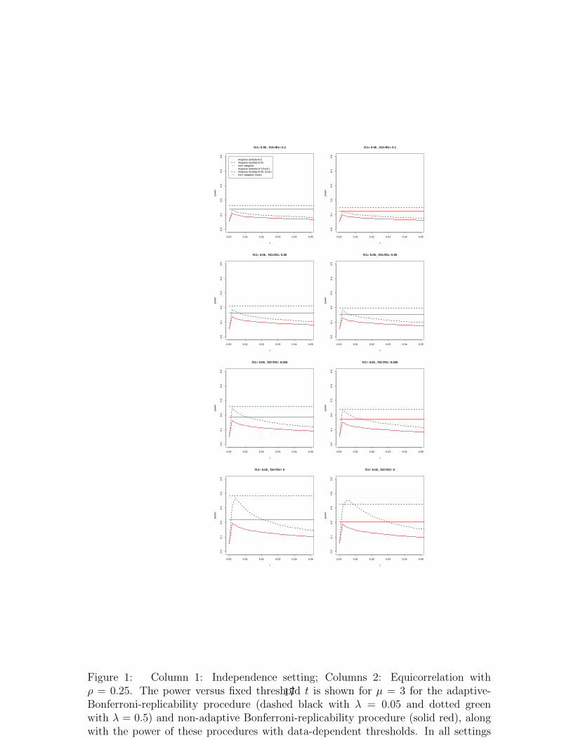
Figure 1 shows the power for various fixed selection thresholds t1 = t2 = t. There isa clear gain from adaptivity since the power curves for the adaptive procedures areabove those for the non-adaptive procedures, for the same fixed threshold t. The gainfrom adaptivity is larger as the difference between f11 and f10 = f01 is larger: whilein the last two rows (where f10 = f01 < f11) the power advantage can be greaterthan 10%, in the first row (where f10 = f01 = 0.1, f11 = 0.05) there is almost nopower advantage. The choice of t matters, and the power of the procedures withdata-dependent thresholds (t∗1, t

∗2) is close to the power of the procedures with the

best possible fixed threshold t.

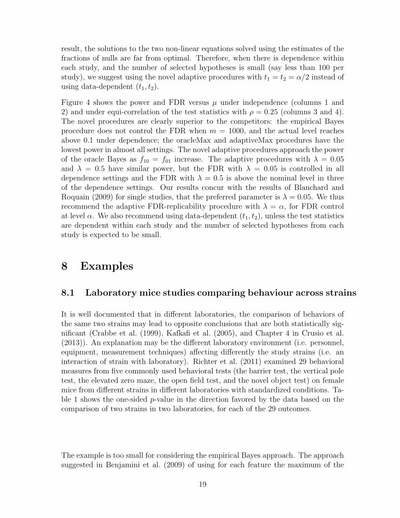
Figure 2 shows the power and FWER versus µ under independence (columns 1 and2) and under equi-correlation of the test statistics with ρ = 0.25 (columns 3 and 4).The novel procedures are clearly superior to the Max and Oracle Max procedures,the adaptive procedures are superior to the non-adaptive variants, and the power ofthe adaptive procedures with data-dependent thresholds is close to that of the oracleBonferroni procedure. The adaptive procedures with λ = 0.05 and λ = 0.5 havesimilar power, but the FWER with λ = 0.05 is controlled in all dependence settingswhile the FWER with λ = 0.5 is above 0.1 in all but the last dependence setting. Ourresults concur with the results of Blanchard and Roquain (2009) for single studies,that the preferred parameter is λ = 0.05. The adaptive procedure with λ = 0.05 anddata-dependent selection thresholds is clearly superior to the two adaptive procedureswith fixed selection thresholds of t1 = t2 = 0.025 or t1 = t2 = 0.049. We thusrecommend the adaptive-Bonferroni-replicability procedure with λ = 0.05 and data-

15

dependent selection thresholds.

7.2 Results for FDR controlling procedures

We considered the following novel procedures for replicability analysis with α =0.05, α1 = 0.025: Non-adaptive-FDR-replicability with fixed or data-dependent (t1, t2);adaptive-FDR-replicability with λ ∈ {0.05, 0.5} and fixed or data-dependent (t1, t2).

Heller and Yekutieli (2014) introduced the oracle Bayes procedure (oracleBayes), andshowed that it has the largest rejection region while controlling the Bayes FDR. Whenm is large and the data is generated from the mixture model, the Bayes FDR coincideswith the frequentist FDR, so oracle Bayes is optimal for FDR control. We consideredthis oracle procedure for comparison with our novel procedures. The difference inpower between the oracle Bayes and the novel frequentist procedures shows howmuch worse our procedures, which make no mixture-model assumptions, are fromthe (best yet unknown in practice) oracle procedure, which assumes the mixturemodel and needs as input its parameters. In addition, the following three procedureswere considered: the empirical Bayes procedure (eBayes), as implemented in the Rpackage repfdr (Heller et al., 2014b), which estimates the Bayes FDR and rejectsthe features with estimated Bayes FDR below α, see Heller and Yekutieli (2014) fordetails; the oracle BH on {max(p1i, p2i) : i = 1, . . . ,m} (oracleMax); and the adaptiveBH on {max(p1i, p2i) : i = 1, . . . ,m} (adaptiveMax). Specifics about oracleMaxand adaptiveMax follow. Applying the BH on {max(p1i, p2i) : i = 1, . . . ,m} atlevel x, it is easy to show that the FDR level for independent features is at mostf00x

2 + (1 − f00 − f11)x. Therefore, the oracleMax procedure uses level x, which isthe solution to f00x

2 + (1− f00 − f11)x = 0.05, and the adaptiveMax procedure useslevel x, which is the solution to f̂00x

2 + (1− f̂00− f̂11)x = 0.05, where f̂00 and f̂11 arethe estimated mixture fractions computed using the R package repfdr.

Figure 3 shows the power of novel procedures for various fixed selection thresholdst1 = t2 = t, as well as for the variants with data-dependent thresholds. There is a cleargain from adaptivity since the power curves for the adaptive procedures are abovethose for the non-adaptive procedures, for the same fixed threshold t. The choice of tmatters, and the choice t = 0.025 is better than the choice t = 0.05, and fairly close tothe best t. We see that the power of the non-adaptive procedures with data-dependentselection thresholds is superior to the power of non-adaptive procedures with fixedthresholds. The same is true for the adaptive procedures in all the settings exceptfor the last two rows of the equi-correlation setting, where the power of the adaptiveprocedures with data-dependent thresholds is slightly lower than the highest powerfor fixed thresholds t1 = t2 = t. In these settings the number of selected hypothesesis on average lower than in other settings, and the fractions of true null hypothesesin one study among the selected in the other study are expected to be small. As a

16

0.00 0.01 0.02 0.03 0.04 0.05

0.0

0.1

0.2

0.3

0.4

0.5

f11= 0.05 , f10=f01= 0.1

t

pow

er

Adaptive lambda=0.5Adaptive lambda=0.05Non−adaptiveAdaptive lambda=0.5,fixed tAdaptive lambda=0.05, fixed tNon−adaptive, fixed t

0.00 0.01 0.02 0.03 0.04 0.05

0.0

0.1

0.2

0.3

0.4

0.5

f11= 0.05 , f10=f01= 0.1

t

pow

er

0.00 0.01 0.02 0.03 0.04 0.05

0.0

0.1

0.2

0.3

0.4

0.5

f11= 0.05 , f10=f01= 0.05

t

pow

er

0.00 0.01 0.02 0.03 0.04 0.05

0.0

0.1

0.2

0.3

0.4

0.5

f11= 0.05 , f10=f01= 0.05

t

pow

er

0.00 0.01 0.02 0.03 0.04 0.05

0.0

0.1

0.2

0.3

0.4

0.5

f11= 0.05 , f10=f01= 0.025

t

pow

er

0.00 0.01 0.02 0.03 0.04 0.05

0.0

0.1

0.2

0.3

0.4

0.5

f11= 0.05 , f10=f01= 0.025

t

pow

er

0.00 0.01 0.02 0.03 0.04 0.05

0.0

0.1

0.2

0.3

0.4

0.5

f11= 0.05 , f10=f01= 0

t

pow

er

0.00 0.01 0.02 0.03 0.04 0.05

0.0

0.1

0.2

0.3

0.4

0.5

f11= 0.05 , f10=f01= 0

t

pow

er

Figure 1: Column 1: Independence setting; Columns 2: Equicorrelation withρ = 0.25. The power versus fixed threshold t is shown for µ = 3 for the adaptive-Bonferroni-replicability procedure (dashed black with λ = 0.05 and dotted greenwith λ = 0.5) and non-adaptive Bonferroni-replicability procedure (solid red), alongwith the power of these procedures with data-dependent thresholds. In all settingsm = 1000, α = 0.05, α1 = 0.025.

17

2.5 3.0 3.5 4.0 4.5 5.0 5.5

0.0

0.2

0.4

0.6

0.8

1.0

f11= 0.05 , f10=f01= 0.1

mu

pow

er

Adaptive lambda=0.5Adaptive lambda=0.05Non−adaptiveOracle Oracle maxAdaptive maxAdaptive lambda=0.05,t=0.049Adaptive lambda=0.05,t=0.025

2.5 3.0 3.5 4.0 4.5 5.0 5.5

0.0

00

.05

0.1

00

.15

0.2

0

f11= 0.05 , f10=f01= 0.1

mu

FW

ER

2.5 3.0 3.5 4.0 4.5 5.0 5.5

0.0

0.2

0.4

0.6

0.8

1.0

f11= 0.05 , f10=f01= 0.1

mu

pow

er

2.5 3.0 3.5 4.0 4.5 5.0 5.5

0.0

00

.05

0.1

00

.15

0.2

0

f11= 0.05 , f10=f01= 0.1

mu

FW

ER

2.5 3.0 3.5 4.0 4.5 5.0 5.5

0.0

0.2

0.4

0.6

0.8

1.0

f11= 0.05 , f10=f01= 0.05

mu

pow

er

2.5 3.0 3.5 4.0 4.5 5.0 5.5

0.0

00

.05

0.1

00

.15

0.2

0

f11= 0.05 , f10=f01= 0.05

mu

FW

ER

2.5 3.0 3.5 4.0 4.5 5.0 5.5

0.0

0.2

0.4

0.6

0.8

1.0

f11= 0.05 , f10=f01= 0.05

mu

pow

er

2.5 3.0 3.5 4.0 4.5 5.0 5.5

0.0

00

.05

0.1

00

.15

0.2

0

f11= 0.05 , f10=f01= 0.05

mu

FW

ER

2.5 3.0 3.5 4.0 4.5 5.0 5.5

0.0

0.2

0.4

0.6

0.8

1.0

f11= 0.05 , f10=f01= 0.025

mu

pow

er

2.5 3.0 3.5 4.0 4.5 5.0 5.5

0.0

00

.05

0.1

00

.15

0.2

0

f11= 0.05 , f10=f01= 0.025

mu

FW

ER

2.5 3.0 3.5 4.0 4.5 5.0 5.5

0.0

0.2

0.4

0.6

0.8

1.0

f11= 0.05 , f10=f01= 0.025

mu

pow

er

2.5 3.0 3.5 4.0 4.5 5.0 5.5

0.0

00

.05

0.1

00

.15

0.2

0

f11= 0.05 , f10=f01= 0.025

mu

FW

ER

2.5 3.0 3.5 4.0 4.5 5.0 5.5

0.0

0.2

0.4

0.6

0.8

1.0

f11= 0.05 , f10=f01= 0

mu

pow

er

2.5 3.0 3.5 4.0 4.5 5.0 5.5

0.0

00

.05

0.1

00

.15

0.2

0

f11= 0.05 , f10=f01= 0

mu

FW

ER

2.5 3.0 3.5 4.0 4.5 5.0 5.5

0.0

0.2

0.4

0.6

0.8

1.0

f11= 0.05 , f10=f01= 0

mu

pow

er

2.5 3.0 3.5 4.0 4.5 5.0 5.5

0.0

00

.05

0.1

00

.15

0.2

0

f11= 0.05 , f10=f01= 0

mu

FW

ER

Figure 2: Columns 1 and 2: Independence setting; Columns 3 and 4: Equi-correlation with ρ = 0.25. Powerand FWER versus µ for the adaptive-Bonferroni-replicability procedure with data-dependent (t1, t2) with λ = 0.5(solid black ) and with λ = 0.05 (dashed black); Bonferroni-replicability procedure with data-dependent (t1, t2)(dotted black); the oracle that knows which hypotheses are null in one study among the selected from the otherstudy (dashed blue); oracle Max (dotted blue) and Max (dotted red); adaptive-Bonferroni-replicability with fixedλ = 0.05 and fixed t1 = t2 = 0.049 (dash-dot green) and fixed t1 = t2 = 0.025 (dash green). In all settings m = 1000,α = 0.05, α1 = 0.025.

18

result, the solutions to the two non-linear equations solved using the estimates of thefractions of nulls are far from optimal. Therefore, when there is dependence withineach study, and the number of selected hypotheses is small (say less than 100 perstudy), we suggest using the novel adaptive procedures with t1 = t2 = α/2 instead ofusing data-dependent (t1, t2).

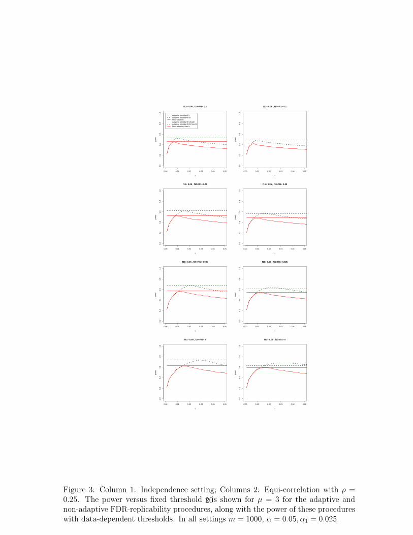
Figure 4 shows the power and FDR versus µ under independence (columns 1 and2) and under equi-correlation of the test statistics with ρ = 0.25 (columns 3 and 4).The novel procedures are clearly superior to the competitors: the empirical Bayesprocedure does not control the FDR when m = 1000, and the actual level reachesabove 0.1 under dependence; the oracleMax and adaptiveMax procedures have thelowest power in almost all settings. The novel adaptive procedures approach the powerof the oracle Bayes as f10 = f01 increase. The adaptive procedures with λ = 0.05and λ = 0.5 have similar power, but the FDR with λ = 0.05 is controlled in alldependence settings and the FDR with λ = 0.5 is above the nominal level in threeof the dependence settings. Our results concur with the results of Blanchard andRoquain (2009) for single studies, that the preferred parameter is λ = 0.05. We thusrecommend the adaptive FDR-replicability procedure with λ = α, for FDR controlat level α. We also recommend using data-dependent (t1, t2), unless the test statisticsare dependent within each study and the number of selected hypotheses from eachstudy is expected to be small.

8 Examples

8.1 Laboratory mice studies comparing behaviour across strains

It is well documented that in different laboratories, the comparison of behaviors ofthe same two strains may lead to opposite conclusions that are both statistically sig-nificant (Crabbe et al. (1999), Kafkafi et al. (2005), and Chapter 4 in Crusio et al.(2013)). An explanation may be the different laboratory environment (i.e. personnel,equipment, measurement techniques) affecting differently the study strains (i.e. aninteraction of strain with laboratory). Richter et al. (2011) examined 29 behavioralmeasures from five commonly used behavioral tests (the barrier test, the vertical poletest, the elevated zero maze, the open field test, and the novel object test) on femalemice from different strains in different laboratories with standardized conditions. Ta-ble 1 shows the one-sided p-value in the direction favored by the data based on thecomparison of two strains in two laboratories, for each of the 29 outcomes.

The example is too small for considering the empirical Bayes approach. The approachsuggested in Benjamini et al. (2009) of using for each feature the maximum of the

19

0.00 0.01 0.02 0.03 0.04 0.05

0.0

0.2

0.4

0.6

0.8

1.0

f11= 0.05 , f10=f01= 0.1

t

pow

er

Adaptive lambda=0.5Adaptive lambda=0.05Non−adaptiveAdaptive lambda=0.5,fixed tAdaptive lambda=0.05, fixed tNon−adaptive, fixed t

0.00 0.01 0.02 0.03 0.04 0.05

0.0

0.2

0.4

0.6

0.8

1.0

f11= 0.05 , f10=f01= 0.1

t

pow

er

0.00 0.01 0.02 0.03 0.04 0.05

0.0

0.2

0.4

0.6

0.8

1.0

f11= 0.05 , f10=f01= 0.05

t

pow

er

0.00 0.01 0.02 0.03 0.04 0.05

0.0

0.2

0.4

0.6

0.8

1.0

f11= 0.05 , f10=f01= 0.05

t

pow

er

0.00 0.01 0.02 0.03 0.04 0.05

0.0

0.2

0.4

0.6

0.8

1.0

f11= 0.05 , f10=f01= 0.025

t

pow

er

0.00 0.01 0.02 0.03 0.04 0.05

0.0

0.2

0.4

0.6

0.8

1.0

f11= 0.05 , f10=f01= 0.025

t

pow

er

0.00 0.01 0.02 0.03 0.04 0.05

0.0

0.2

0.4

0.6

0.8

1.0

f11= 0.05 , f10=f01= 0

t

pow

er

0.00 0.01 0.02 0.03 0.04 0.05

0.0

0.2

0.4

0.6

0.8

1.0

f11= 0.05 , f10=f01= 0

t

pow

er

Figure 3: Column 1: Independence setting; Columns 2: Equi-correlation with ρ =0.25. The power versus fixed threshold t is shown for µ = 3 for the adaptive andnon-adaptive FDR-replicability procedures, along with the power of these procedureswith data-dependent thresholds. In all settings m = 1000, α = 0.05, α1 = 0.025.

20

2.5 3.0 3.5 4.0 4.5 5.0 5.5

0.0

0.2

0.4

0.6

0.8

1.0

f11= 0.05 , f10=f01= 0.1

mu

pow

er Adaptive lambda=0.5

Adaptive lambda=0.05Non−adaptiveoracle BayesOracle maxEmpirical BayesAdaptive maxAdaptive lambda=0.05,t=0.049Adaptive lambda=0.05,t=0.025

2.5 3.0 3.5 4.0 4.5 5.0 5.5

0.0

00

.05

0.1

00

.15

0.2

0

f11= 0.05 , f10=f01= 0.1

muF

DR

2.5 3.0 3.5 4.0 4.5 5.0 5.5

0.0

0.2

0.4

0.6

0.8

1.0

f11= 0.05 , f10=f01= 0.1

mu

pow

er

2.5 3.0 3.5 4.0 4.5 5.0 5.5

0.0

00

.05

0.1

00

.15

0.2

0

f11= 0.05 , f10=f01= 0.1

mu

FD

R

2.5 3.0 3.5 4.0 4.5 5.0 5.5

0.0

0.2

0.4

0.6

0.8

1.0

f11= 0.05 , f10=f01= 0.05

mu

pow

er

2.5 3.0 3.5 4.0 4.5 5.0 5.5

0.0

00

.05

0.1

00

.15

0.2

0

f11= 0.05 , f10=f01= 0.05

mu

FD

R

2.5 3.0 3.5 4.0 4.5 5.0 5.5

0.0

0.2

0.4

0.6

0.8

1.0

f11= 0.05 , f10=f01= 0.05

mu

pow

er

2.5 3.0 3.5 4.0 4.5 5.0 5.5

0.0

00

.05

0.1

00

.15

0.2

0

f11= 0.05 , f10=f01= 0.05

mu

FD

R

2.5 3.0 3.5 4.0 4.5 5.0 5.5

0.0

0.2

0.4

0.6

0.8

1.0

f11= 0.05 , f10=f01= 0.025

mu

pow

er

2.5 3.0 3.5 4.0 4.5 5.0 5.5

0.0

00

.05

0.1

00

.15

0.2

0

f11= 0.05 , f10=f01= 0.025

mu

FD

R

2.5 3.0 3.5 4.0 4.5 5.0 5.5

0.0

0.2

0.4

0.6

0.8

1.0

f11= 0.05 , f10=f01= 0.025

mu

pow

er

2.5 3.0 3.5 4.0 4.5 5.0 5.5

0.0

00

.05

0.1

00

.15

0.2

0

f11= 0.05 , f10=f01= 0.025

mu

FD

R

2.5 3.0 3.5 4.0 4.5 5.0 5.5

0.0

0.2

0.4

0.6

0.8

1.0

f11= 0.05 , f10=f01= 0

mu

pow

er

2.5 3.0 3.5 4.0 4.5 5.0 5.5

0.0

00

.05

0.1

00

.15

0.2

0

f11= 0.05 , f10=f01= 0

mu

FD

R

2.5 3.0 3.5 4.0 4.5 5.0 5.5

0.0

0.2

0.4

0.6

0.8

1.0

f11= 0.05 , f10=f01= 0

mu

pow

er

2.5 3.0 3.5 4.0 4.5 5.0 5.5

0.0

00

.05

0.1

00

.15

0.2

0

f11= 0.05 , f10=f01= 0

mu

FD

R

Figure 4: Columns 1 and 2: Independence setting; Columns 3 and 4: Equi-correlation with ρ = 0.25. Power andFDR versus µ for the adaptive-FDR-replicability procedure with data-dependent (t1, t2) with λ = 0.5 (solid black)and with λ = 0.05 (dashed black); Non-adaptive-FDR-replicability procedure with data-dependent (t1, t2) (dottedblack); the oracle Bayes (dashed blue) and empirical Bayes (dashed red); the oracle and adaptive BH on maximump-value, (dotted blue and dotted red); adaptive-FDR-replicability procedure with λ = 0.05 and fixed t1 = t2 = 0.049(dash-dot green) and fixed t1 = t2 = 0.025 (dash green). In all settings m = 1000, α = 0.05, α1 = 0.025.

21

Table 1: For 16 female mice from each of two inbred strains, ” C57BL6NCrl” and ”DBA/2NCrl”, in each of twolaboratories, the Wilcoxon rank sum test one-sided p-value was computed for the test of no association between strainand behavioral endpoint. We show the p-values for the lab of H. Wurbel at the University of Giessen in column 3,and for the lab of P. Gass at the Central Institute of Mental Health, Mannheim in column 4. The direction of thealternative favored by the data is shown in column 2, and it is marked as ”X” if the laboratories differ in the directionof smallest one-sided p-value. The rows are the outcomes from 5 behavioural tests: the barrier test (row 1); thevertical pole test (row 2); the elevated zero maze (rows 3-11) ; the open field test (rows 12-19); the novel object test(rows 20-29).

min(PLij , PRij )

Alternative i = 1 i = 21 X 0.3161 0.02182 C57BL < DBA 0.0012 0.00003 X 0.0194 0.11204 C57BL < DBA 0.0095 0.29485 C57BL < DBA 0.1326 0.00286 C57BL > DBA 0.1488 0.00037 C57BL > DBA 0.2248 0.00008 X 0.4519 0.00059 C57BL < DBA 0.0061 0.000010 C57BL < DBA 0.0071 0.088811 X 0.4297 0.160212 C57BL < DBA 0.0918 0.050613 X 0.0918 0.000114 C57BL < DBA 0.0000 0.004815 X 0.0005 0.0550

min(PLij , PRij )

Alternative i = 1 i = 216 C57BL < DBA 0.0059 0.000217 C57BL > DBA 0.0176 0.000318 X 0.0000 0.053819 C57BL < DBA 0.0000 0.172720 C57BL < DBA 0.0157 0.000121 C57BL < DBA 0.0000 0.023422 C57BL < DBA 0.3620 0.017623 C57BL < DBA 0.0000 0.000124 C57BL < DBA 0.0000 0.007625 C57BL < DBA 0.0000 0.000026 C57BL < DBA 0.0000 0.000327 C57BL < DBA 0.0000 0.000128 C57BL < DBA 0.0000 0.055029 X 0.0033 0.3760

two studies p-values, i.e., 2 min{max(pL1j, pL2j),max(pR1j, p

R2j)}, detected overall fewer

outcomes than using our novel procedures both for FWER and for FDR control.

Table 2 shows the FWER/FDR non-adaptive and adaptive r-values, for the selectedfeatures, according to the rule which selects all features with two-sided p-values thatare at most 0.05. We did not consider data-dependent thresholds since the number offeatures examined was only 29, which could result in highly variable data-dependentthresholds and a power loss comparing to procedures with fixed thresholds, as wasobserved in simulations. At the α = 0.05 level, for FWER control, four discoverieswere made by using Bonferroni on the maximum p-values, and five discoveries weremade with the non-adaptive and adaptive Bonferroni-replicability procedures. Atthe α = 0.05 level, for FDR control, nine discoveries were made by using BH onthe maximum p-values, and nine and twelve discoveries were made with the non-adaptive FDR and adaptive FDR-replicability procedures, respectively. Note thatthe adaptive r-values can be less than half the non-adaptive r-values, since π̂I0 = 0.44and π̂II0 = 0.47.

8.2 Microarray studies comparing groups with different can-cer severity

Freije et al. (2004) and Phillips et al. (2004) compared independently the expressionlevels in patients with grade III and grade IV brain cancer. Both studies used

22

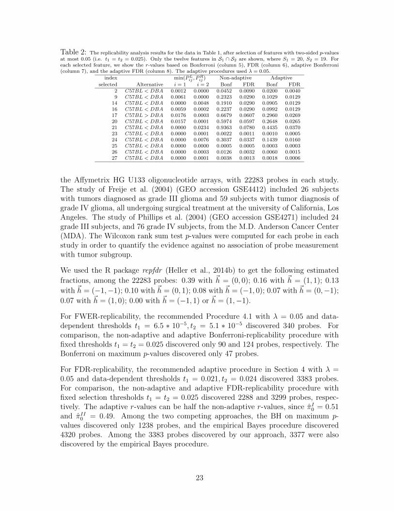
Table 2: The replicability analysis results for the data in Table 1, after selection of features with two-sided p-valuesat most 0.05 (i.e. t1 = t2 = 0.025). Only the twelve features in S1 ∩ S2 are shown, where S1 = 20, S2 = 19. Foreach selected feature, we show the r-values based on Bonferroni (column 5), FDR (column 6), adaptive Bonferroni(column 7), and the adaptive FDR (column 8). The adaptive procedures used λ = 0.05.

index min(PLij , PRij ) Non-adaptive Adaptive

selected Alternative i = 1 i = 2 Bonf FDR Bonf FDR2 C57BL < DBA 0.0012 0.0000 0.0452 0.0090 0.0200 0.00409 C57BL < DBA 0.0061 0.0000 0.2323 0.0290 0.1029 0.0129

14 C57BL < DBA 0.0000 0.0048 0.1910 0.0290 0.0905 0.012916 C57BL < DBA 0.0059 0.0002 0.2237 0.0290 0.0992 0.012917 C57BL > DBA 0.0176 0.0003 0.6679 0.0607 0.2960 0.026920 C57BL < DBA 0.0157 0.0001 0.5974 0.0597 0.2648 0.026521 C57BL < DBA 0.0000 0.0234 0.9363 0.0780 0.4435 0.037023 C57BL < DBA 0.0000 0.0001 0.0022 0.0011 0.0010 0.000524 C57BL < DBA 0.0000 0.0076 0.3037 0.0337 0.1439 0.016025 C57BL < DBA 0.0000 0.0000 0.0005 0.0005 0.0003 0.000326 C57BL < DBA 0.0000 0.0003 0.0126 0.0032 0.0060 0.001527 C57BL < DBA 0.0000 0.0001 0.0038 0.0013 0.0018 0.0006

the Affymetrix HG U133 oligonucleotide arrays, with 22283 probes in each study.The study of Freije et al. (2004) (GEO accession GSE4412) included 26 subjectswith tumors diagnosed as grade III glioma and 59 subjects with tumor diagnosis ofgrade IV glioma, all undergoing surgical treatment at the university of California, LosAngeles. The study of Phillips et al. (2004) (GEO accession GSE4271) included 24grade III subjects, and 76 grade IV subjects, from the M.D. Anderson Cancer Center(MDA). The Wilcoxon rank sum test p-values were computed for each probe in eachstudy in order to quantify the evidence against no association of probe measurementwith tumor subgroup.

We used the R package repfdr (Heller et al., 2014b) to get the following estimated

fractions, among the 22283 probes: 0.39 with ~h = (0, 0); 0.16 with ~h = (1, 1); 0.13

with ~h = (−1,−1); 0.10 with ~h = (0, 1); 0.08 with ~h = (−1, 0); 0.07 with ~h = (0,−1);

0.07 with ~h = (1, 0); 0.00 with ~h = (−1, 1) or ~h = (1,−1).

For FWER-replicability, the recommended Procedure 4.1 with λ = 0.05 and data-dependent thresholds t1 = 6.5 ∗ 10−5, t2 = 5.1 ∗ 10−5 discovered 340 probes. Forcomparison, the non-adaptive and adaptive Bonferroni-replicability procedure withfixed thresholds t1 = t2 = 0.025 discovered only 90 and 124 probes, respectively. TheBonferroni on maximum p-values discovered only 47 probes.

For FDR-replicability, the recommended adaptive procedure in Section 4 with λ =0.05 and data-dependent thresholds t1 = 0.021, t2 = 0.024 discovered 3383 probes.For comparison, the non-adaptive and adaptive FDR-replicability procedure withfixed selection thresholds t1 = t2 = 0.025 discovered 2288 and 3299 probes, respec-tively. The adaptive r-values can be half the non-adaptive r-values, since π̂I0 = 0.51and π̂II0 = 0.49. Among the two competing approaches, the BH on maximum p-values discovered only 1238 probes, and the empirical Bayes procedure discovered4320 probes. Among the 3383 probes discovered by our approach, 3377 were alsodiscovered by the empirical Bayes procedure.

23

9 Discussion

In this paper we proposed novel procedures for establishing replicability in two stud-ies. First, we introduced procedures that take the selected set of features in eachof two studies, and infer about the replicability of features selected in both studieswhile controlling for false replicability claims. We proved that the FWER controllingprocedure is valid (i.e., controls the error rate at the desired nominal level) for anydependence within each study, and that the FDR controlling procedure is valid un-der independence of the test statistics within each study, and suggested also a moreconservative procedure that is valid for arbitrary dependence. Next, we suggestedincorporating the plug-in estimates of the fraction of nulls in one study among theselected features by the other study, which can be estimated as long as the p-valuesfor the union of features selected is available. We proved that the resulting adap-tive FWER and FDR controlling procedures are valid under independence of the teststatistics within each study. Our empirical investigations showed that the adaptiveprocedures remain valid even when the independence assumption is violated, as longas we use λ = α as a parameter for the plug-in estimates, as suggested by Blanchardand Roquain (2009) for the adaptive BH procedure. Finally, when two full studies areavailable that examine the same features, we suggested selecting features for replica-bility analysis that have p-values below certain thresholds. We showed that selectingthe features with one-sided p-values below α/2 has good power, but that the powercan further be improved if we use data-dependent thresholds, which receive the valuesthat will lead to the procedure selecting exactly the features that are discovered ashaving replicated findings.

Our practical guidelines for establishing replicability are to use the adaptive proce-dure for the desired error rate control, with λ = α. Moreover, based on the simulationresults we suggest using the data-dependent selection thresholds when two full studiesare available if the number of selected features in each study is expected to be largeenough (say above 100), and using the fixed thresholds t1 = t2 = α/2 otherwise. Wewould like to note that the r-value computation is more involved when the thresholdsare data-dependent, since these thresholds depend on the nominal level α. An inter-esting open question is how to account for multiple solutions of the two non-linearequations that are solved in order to find the data-dependent thresholds.

The suggested procedures can be generalized to the case that more than two studiesare available. It is possible to either aggregate multiple results of pairwise replicabilityanalyses, or to first aggregate the data and then apply a single replicability analysis ontwo meta-analysis p-values. The aim of the replicability analysis may also be redefinedto be that of discovering features that have replicated findings in at least u studies,where u can range from two to the total number of studies. Other extensions includeweighting the features differently, as suggested by Genovese et al. (2006), based onprior knowledge on the features, and replicability analysis on multiple families ofhypotheses while controlling more general error rates, as suggested by Benjamini andBogomolov (2013).

24

References

Benjamini, Y. and Bogomolov, M. (2013). Selective inference on multiple familiesof hypotheses. Journal of the Royal Statistical Society. Series B (Methodological),76(1):297–318.

Benjamini, Y., Heller, R., and Yekutieli, D. (2009). Selective inference in complexresearch. Philosophical Transactions of the Royal Society A, 267:1–17.

Benjamini, Y. and Hochberg, Y. (1995). Controlling the false discovery rate - apractical and powerful approach to multiple testing. Journal of the Royal StatisticalSociety. Series B (Methodological), 57 (1):289–300.

Benjamini, Y. and Hochberg, Y. (2000). On the adaptive control of the false discoveryfate in multiple testing with independent statistics. Journal of Educational andBehavioral Statistics, 25(1):60–83.

Benjamini, Y., Krieger, M., and Yekutieli, D. (2006). Adaptive linear step-up falsediscovery rate controlling procedures. Biometrika, 93 (3):491–507.

Blanchard, G. and Roquain, E. (2009). Adaptive false discovery rate control underindependence and dependence. Journal of Machine Learning Research, 10:2837–2871.

Bogomolov, M. and Heller, R. (2013). Discovering findings that replicate from aprimary study of high dimension to a follow-up study. Journal of the AmericanStatistical Association, 108(504):1480–1492.

Crabbe, J., Wahlsten, D., and Dudek, B. (1999). Genetics of mouse behavior: inter-actions with laboratory environment. Science, 284 (5420):1670–1672.

Crusio, W., Sluyter, F., Gerlai, R., and Pietropaolo, S. (2013). Behavioral Genetics ofthe Mouse: Genetics of Behavioral Phenotypes., volume 1. Cambridge Handbooksin Behavioral Genetics.

Dickhaus, T., Strassburger, K., Schunk, D., Morcillo-Suarez, C., Illig, T., andNavarro, A. (2012). How to analyze many contingency tables simultaneously ingenetic association studies. Statistical Applications in Genetics and Molecular Bi-ology, 11(4).

Finner, H. and Gontsharuk, V. (2009). Controlling the familywise error rate withplug-in estimator for the proportion of true null hypotheses. Journal of the RoyalStatistical Society. Series B (Methodological), 71 (5):1031–1048.

Freije et al. (2004). Gene expression profiling of gliomas strongly predicts survival.Cancer Res, 15(64):6503–6510.

Genovese, C., Roeder, K., and Wasserman, L. (2006). False discovery control withp-value weighting. Biometrika, 93 (3):509–524.

25

Heller, R., Bogomolov, M., and Benjamini, Y. (2014a). Deciding whether follow-upstudies have replicated findings in a preliminary large-scale ’omics’ study. Proceed-ings of the National Academy of Sciences.

Heller, R., Yaacoby, S., and Yekutieli, D. (2014b). repfdr: A tool for replicabilityanalysis for genome-wide association studies. Bioinformatics, 30(20):2971–2972.

Heller, R. and Yekutieli, D. (2014). Replicability analysis for genome-wide associationstudies. The Annals of Applied Statistics, 8(1):481–498.

Kafkafi, N., Benjamini, Y., Sakov, A., Elmer, G., and Golani, I. (2005). Genotype-environment interactions in mouse behavior: a way out of the problem. Proceedingsof the National Academy of Sciences, 102 (12):4619–4624.

Li, Q., Brown, J., Huang, H., and Bickel, P. (2014). Measuring reproducibility ofhigh-throughput experiments. The Annals of Applied Statistics, 5(3):1752–1779.

Phillips et al. (2004). Molecular subclasses of high-grade glioma predict prognosis,delineate a pattern of disease progression, and resemble stages in neurogenesis.Cancer Cell, 9(3):157–173.

Reiner, A., Yekutieli, D., and Benjamini, Y. (2003). Identifying differentially ex-pressed genes using false discovery rate controlling procedures. Bioinformatics,19(3):368–375.

Richter et al. (2011). Effect of population heterogenization on the reproducibility ofmouse behavior: A multi-laboratory study. PLoS ONE, 6(1).

Schweder, P. and Spjotvoll, E. (1982). Plots of p-values to evaluate many testssimultaneously. Biometrika, 69:493–502.

Storey, J. (2003). The positive false discovery rate: a bayesian interpretation and theq-value. Annals of Statistics, 31:2013–2035.

Wright, S. (1992). Adjusted p-values for simultaneous inference. Biometrics,48(4):1005–1013.

A Notation for technical derivations

For the technical derivations, the following notation will be used. Let pi be the m-dimensional vector of p-values for study i, Si(pi) be the index set of features selectedfrom study i based on the vector of p-values pi, and Si(pi) be the cardinality of this

set, for i ∈ {1, 2}. Let P(j)i = (Pi1, . . . , Pi,j−1, Pi,j+1, . . . , Pim) be the vector of p-values

for the m − 1 features excluding j, for i = 1, 2. When the selection rule by whichthe set Si is selected is stable, define S(j)

i ⊆ {1, . . . , j − 1, j + 1, . . . ,m} as the set of

26

indices selected along with j, if j ∈ Si, and S(j)i,λ as S(j)

i ∩ {l 6= j : Pil ≤ λ} if j ∈ Si,λ,for i ∈ {1, 2}, and let S

(j)i = |S(j)

i |. Define S(j)i (ti) = {l : pil ≤ ti, l 6= j} as the

index set of features with p-value at most ti from the vector of p-values p(j)i , and let

S(j)i (ti) = |S(j)

i (ti)|. For c ∈ (0, 1), we write α1 = cα and α2 = α− α1.

B Proof of Theorems 3.2 and 4.2

In the proofs of Theorems 3.2 and 4.2 we use the following lemma. The lemma isproven in the end of the section.

Lemma B.1. Let Si be the selected set of features based on study i, for i = 1, 2. Letrj, j ∈ S1 ∩ S2 be the Bonferroni-type r-values:

rj = max

{W1p1j

c,W2p2j

1− c

}, j ∈ S1 ∩ S2, (B.1)

where c ∈ (0, 1) is a constant and W1,W2 may be constants or random variables basedon p-values. The FDR r-values based on the Bonferroni-type r-values are:

rFDRj = min{i: ri≥rj ,i∈S1∩S2}

rirank(ri)

, j ∈ S1 ∩ S2,

where rank(ri) is the rank of the Bonferroni-type r-value for feature i ∈ S1 ∩S2, withmaximum rank for ties.

(1) The procedure that declares as replicated the features with FDR r-values at mostα is equivalent to the following procedure on the selected features S1 ∩ S2:

(a) Let

R , max

{r :

∑j∈S1∩S2

I

[(p1j, p2j) ≤

(rα1

W1

,rα2

W2

)]= r

}.

(b) The set of indices with replicability claims is

R = {j : (p1j, p2j) ≤(Rα1

W1

,Rα2

W2

), j ∈ S1 ∩ S2}.

(2) The procedure that declares as replicated the features with FDR r-values at mostα controls the FDR for replicability analysis at level α if the following conditionsare satisfied:

(a) The p-values corresponding to true null hypotheses are each independentof all the other p-values.

27

(b) For each j ∈ {1, . . . ,m}, there exist random variables (or constants) W(j)1 ,W

(j)2

defined on the space (P(j)1 , P

(j)2 ) such that if j ∈ S1 ∩ S2, then W1 = W

(j)1 ,

W2 = W(j)2 ,and for arbitrary fixed vectors p1and p2 it holds:

I[j ∈ S2(p2)]E(1/W(j)1 |P2 = p2) ≤ 1∑

j∈S2(p2)(1−H1j)(B.2)

I[j ∈ S1(p1)]E(1/W(j)2 |P1 = p1) ≤ 1∑

j∈S1(p1)(1−H2j). (B.3)

Proof of item 1 of Theorem 3.2 The result of item 1 of Theorem 3.2 follows fromLemma B.1. The conditions of Lemma B.1 hold with W1 = S2, W

(j)1 = 1 + S

(j)2 , and

W2 = S1, W(j)2 = 1 + S

(j)1 . In order to see it, note that for j ∈ S1 ∩ S2, Si = 1 + S

(j)i

for i ∈ {1, 2}. In addition, note that for arbitrary fixed vector p2 and j ∈ {1, . . . ,m}

I[j ∈ S2(p2)]E

(1

W(j)1

|P2 = p2

)=I[j ∈ S2(p2)]E

(1

1 + S(j)2

|P2 = p2

)

=I[j ∈ S2(p2)]

(1

S2(p2)

)≤ 1∑

j∈S2(p2)(1−H1j).

Thus we have proved inequality (B.2). The proof of inequality (B.3) is similar.

Proof of Theorem 4.2 The result of Theorem 4.2 follows from Lemma B.1. Theconditions of Lemma B.1 hold with Si,λ, i = 1, 2 as the selected sets, and

W1 = S2,λπ̂I0 =

1 +∑

i∈S2,λ I(P1i > λ)

(1− λ), W

(j)1 =

1 +∑

i∈S2,λ,i 6=j I(P1i > λ)

(1− λ),

W2 = S1,λπ̂II0 =

1 +∑

i∈S1,λ I(P2i > λ)

(1− λ), W

(j)2 =

1 +∑

i∈S1,λ,i 6=j I(P2i > λ)

(1− λ).

In order to see it, note that if j ∈ S1,λ ∩ S2,λ, it holds that max{P1j, P2j} ≤ λ. Inaddition, it was shown in the proof of Theorem 4.1 that for arbitrary fixed vector p2

and j ∈ {1, . . . ,m}

I[j ∈ S2,λ(p2)]E

(1

W(j)1

|P2 = p2

)≤

I[j ∈ S2,λ(p2)]E

(1/

(1 +

∑i∈S2,λ,i 6=j(1−H1j)I(P1i > λ)

1− λ

)|P2 = p2

)≤

1∑j∈S2,λ(p2)(1−H1j)

.

The proof of inequality (B.3) is similar.Proof of item 1 of Lemma B.1. Note that the procedure given in item 1 of LemmaB.1 can be written as follows:

28

1. Let

R = max

{r :

∑j∈S1∩S2

I [rj ≤ rα] = r

}.

2. The set of indices with replicability claims is

R = {j : rj ≤ Rα, j ∈ S1 ∩ S2}.

Let r0 = max{r :∑

j∈S1∩S2 I [rj ≤ rα] ≥ r}. We prove that R = r0 by contradic-

tion. From the definitions of r0 and R it follows that if R 6= r0, then r0 > R,and

∑j∈S1∩S2 I [rj ≤ r0α] ≥ r0 + 1. However, since

∑j∈S1∩S2 I [rj ≤ (r0 + 1)α] ≥∑

j∈S1∩S2 I [rj ≤ r0α] it follows that r0 + 1 is also in{r :∑

j∈S1∩S2 I [rj ≤ rα] ≥ r}

,

thus contradicting the definition of r0 as being the greatest value in this set. Thuswe have proved that

R = max

{r :

∑j∈S1∩S2

I [rj ≤ rα] ≥ r

}. (B.4)

We now prove that the procedure that declares as replicated the features with FDRr-values at most α is equivalent to the following procedure in item 1, i.e.

{j : rFDRj ≤ α} = {j : rj ≤ Rα}, (B.5)

where R is given in (B.4). Let us first prove that

{j : rFDRj ≤ α} ⊆ {j : rj ≤ Rα}. (B.6)

Let j ∈ {j : rFDRj ≤ α} be arbitrary fixed. There exists i0 ∈ S1∩S2 such that ri0 ≥ rjand

ri0rank(ri0)

= min{i: ri≥rj ,i∈S1∩S2}

rirank(ri)

≤ α.

Thus ri0 ≤ rank(ri0)α. Therefore, rank(ri0) ≤∑

j∈S1∩S2 I [rj ≤ rank(ri0)α]. Thisinequality and the expression for R given in (B.4) yield that rank(ri0) ≤ R. It followsthat ri0 ≤ Rα. Recall that rj ≤ ri0 , therefore rj ≤ Rα. Thus we have proved (B.6).Let us now prove that

{j : rj ≤ Rα} ⊆ {j : rFDRj ≤ α}. (B.7)

Let j ∈ S1 ∩ S2 be an arbitrary fixed index such that rj ≤ Rα. Since rj ≤ r(R), andr(R)

R≤ α (where r(R) is the R’th largest r-value), it follows that

rFDRj = min{i: ri≥rj ,i∈S1∩S2}

rirank(ri)

≤ α.

Thus we have proved (B.7), which completes the proof of (B.5) and of item 1.

Proof of item 2 of Lemma B.1 For j ∈ {1, . . . ,m} let us define C(j)k as the event

29

in which if rFDRj ≤ α, then the total number of FDR r-values which are at most α

is k. It follows from item 1 and from condition (ii) of item 2 that the event C(j)k is

defined on the space (P(j)1 , P

(j)2 ) as follows. Let

T(j)i =

max

(W

(j)1 p1ic

,W

(j)2 p2i1−c

)if i ∈ S(j)

1 ∩ S(j)2 ,

∞ otherwise.

and let T(j)1 ≤ . . . ≤ T

(j)m−1 be the sorted T -values, where we set T

(j)0 = 0. Note that

T(j)i = ri for i ∈ S(j)

1 ∩ S(j)2 . It follows from the equivalent procedure given in item 1

of Lemma B.1 that

C(j)k = {(P (j)

1 , P(j)2 ) : T

(j)(k−1) ≤ kα, T

(j)(k) > (k + 1)α, . . . , T

(j)(m−1) > mα}. (B.8)

Note that given P1 = p1, for j ∈ S1(p1), C(j)k = ∅ for k > S1(p1), since the number of

finite T(j)i ’s is smaller or equal to S1(p1)− 1. Similarly, given P2 = p2, for j ∈ S2(p2),

C(j)k = ∅ for k > S2(p2). In addition, note that C

(j)k and C

(j)k′ are disjoint events for

any k 6= k′ and∑S1(p1)

k=1 Pr(C(j)k |P1 = p1) =

∑S2(p2)k=1 Pr(C

(j)k |P2 = p2) = 1.

The FDR for replicability analysis is

FDR =m∑j=1

(1−H1jH2j)m∑k=1

1

kPr(j ∈ S1 ∩ S2, r

FDRj ≤ α,C

(j)k

)=

m∑j=1

(1−H1jH2j)m∑k=1

1

kPr(j ∈ S1 ∩ S2, rj ≤ kα,C

(j)k

)(B.9)

≤m∑j=1

(1−H1j)m∑k=1

1

kPr(j ∈ S1 ∩ S2, rj ≤ kα,C

(j)k

)(B.10)

+m∑j=1

(1−H2j)m∑k=1

1

kPr(j ∈ S1 ∩ S2, rj ≤ kα,C

(j)k

)(B.11)

where the equality in (B.9) follows from item 1, and the inequality in (B.10) followsfrom the fact that 1−H1jH2j ≤ 2−H1j−H2j for all j ∈ {1, . . . ,m}. We prove that for(p1, p2) arbitrary fixed, the following inequalities hold for conditional expectations.

m∑j=1

(1−H1j)m∑k=1

1

kPr(j ∈ S1 ∩ S2, rj ≤ kα,C

(j)k |P2 = p2

)≤ α1, (B.12)

m∑j=1

(1−H2j)m∑k=1

1

kPr(j ∈ S1 ∩ S2, rj ≤ kα,C

(j)k |P1 = p1

)≤ α2. (B.13)

Note that since these inequalities hold for all p1 and p2, they yield that the upperbounds in (B.12) and (B.13) hold for expressions in (B.10) and (B.11) respectively,

30

therefore FDR for replicability analysis is upper bounded by α1 + α2 = α. Thus itremains to prove inequalities (B.12) and (B.13). We now prove inequality (B.12).

m∑j=1

(1−H1j)m∑k=1

1

kPr(j ∈ S1 ∩ S2, rj ≤ kα,C

(j)k |P2 = p2

)=

∑j∈S2(p2)

(1−H1j)

S2(p2)∑k=1

1

kPr(j ∈ S1, rj ≤ kα,C

(j)k |P2 = p2

)≤ (B.14)

∑j∈S2(p2)

(1−H1j)

S2(p2)∑k=1

1

kPr

(j ∈ S1, P1j ≤

kcα

W(j)1

, C(j)k |P2 = p2

)≤ (B.15)

α1

∑j∈S2(p2)

(1−H1j)

S2(p2)∑k=1

E

(1

W(j)1

I[C

(j)k

]|P2 = p2

)=

α1

∑j∈S2(p2)

(1−H1j)E

1

W(j)1

S2(p2)∑k=1

I[C

(j)k

]|P2 = p2

= (B.16)

α1

∑j∈S2(p2)

(1−H1j)E

(1

W(j)1

|P2 = p2

)≤ (B.17)

α1

∑j∈S2(p2)

(1−H1j)

(1∑

j∈S2(p2)(1−H1j)

)= α1.

The inequality in (B.14) follows from condition (ii) of item 2. The inequality in(B.15) follows from the fact that the distribution of P1j is uniform or stochasticallylarger than uniform and P1j with H1j = 0 is independent of all other p-values. The

equality in (B.16) follows from the fact that given P2 = p2, ∪S2(p2)k=1 C

(j)k is the whole

sample space represented as a union of disjoint events (as discussed above), therefore∑S2(p2)k=1 I

[C

(j)k

]= 1. The inequality in (B.17) follows from condition (ii) of item

2, inequality (B.2). Thus we proved inequality (B.12). Inequality (B.13) is provedsimilarly.Proof of item 2 in Theorem 3.2. The proof is similar to the proof of item 3 ofTheorem S3.2 in the Supplementary Material of Bogomolov and Heller (2013). We

give it below for completeness. For j, k ∈ {1, . . . ,m}, we define C̃(j)k as the event

in which if r̃FDRj ≤ α, then the total number of arbitrary-dependence FDR r-valueswhich are at most α is k. Similarly to the proof of item 2 of Lemma B.1 it can beshown that the event C̃

(j)k is defined on the space of (P

(j)1 , P

(j)2 ) as in (B.8), where

T -values are replaced by T̃ - values which are defined as follows.

T̃(j)i =

max

((∑S

(j)2 +1

k=1 1/k)(S(j)2 +1)p1i

c,

(∑(S

(j)1 +1)

k=1 1/k)(S(j)1 +1)p2i

1−c

)if i ∈ S(j)

1 ∩ S(j)2 ,

∞ otherwise.

31

Note that T̃(j)i = r̃i for i ∈ S(j)

1 ∩ S(j)2 , where the expression for r̃i is given in (3.2).

Similarly to the proof of item 2 of Lemma B.1, it can be shown that given P1 = p1,C̃

(j)k = ∅ for j ∈ S1(p1) and k > S1(p1), and ∪S1(p1)

k=1 C̃(j)k is the whole sample space.

Given P2 = p2, C̃(j)k = ∅ for j ∈ S2(p2) and k > S2(p2), and ∪S2(p2)

k=1 C̃(j)k is the whole

sample space. In addition, C̃(j)k and C̃

(j)k′ are disjoint events for any k 6= k′.

We obtain the following inequality for the FDR for replicability analysis using deriva-tions (B.9)-(B.11) where we replace rFDRj , rj and C

(j)k by r̃FDRj , r̃j and C̃

(j)k , respec-

tively.

FDR ≤m∑j=1

(1−H1j)m∑k=1

1

kPr(j ∈ S1 ∩ S2, r̃j ≤ kα, C̃

(j)k

)+

m∑j=1

(1−H2j)m∑k=1

1

kPr(j ∈ S1 ∩ S2, r̃j ≤ kα, C̃

(j)k

)(B.18)

We now find an upper bound for the first term of the sum in (B.18). Let p2 be

arbitrary fixed. We define α̃1 = α1/(∑S2(p2)

i=1 1/i). We shall prove that

m∑j=1

(1−H1j)m∑k=1

1

kPr(j ∈ S1 ∩ S2, r̃j ≤ kα, C̃

(j)k |P2 = p2

)≤ α1. (B.19)

Note that

m∑j=1

(1−H1j)m∑k=1

1

kPr(j ∈ S1 ∩ S2, r̃j ≤ kα, C̃

(j)k |P2 = p2

)=

∑j∈S2(p2)

(1−H1j)×

S2(p2)∑k=1

1

kPr

(S1

(S1∑i=1

1/i

)p2j ≤ kα2, j ∈ S1, P1j ≤

kα̃1

S2(p2), C̃

(j)k |P2 = p2

)

≤∑

j∈S2(p2)

(1−H1j)

S2(p2)∑k=1

1

kPr

(P1j ≤

kα̃1

S2(p2), C̃

(j)k |P2 = p2

).

For each j with H1j = 0, k ∈ {1, . . . , S2(p2)}, and l ∈ {1, . . . , k}, let us define:

pjkl = Pr

(P1j ∈

((l − 1)α̃1

S2(p2),lα̃1

S2(p2)

], C̃

(j)k |P2 = p2

).

Note that for j with H1j = 0, Pr (P1j ≤ x) ≤ x for all x ∈ [0, 1], in particularPr (P1j = 0) = 0. Therefore, for each j with H1j = 0 and k ∈ {1, . . . , S2(p2)},

Pr

(P1j ≤

kα̃1

S2(p2), C̃

(j)k |P2 = p2

)=

k∑l=1

pjkl.

32

Using this equality we obtain:∑j∈S2(p2)

(1−H1j)

S2(p2)∑k=1

1

kPr

(P1j ≤

kα̃1

S2(p2), C̃

(j)k |P2 = p2

)=

∑j∈S2(p2)

(1−H1j)

S2(p2)∑k=1

1

k

k∑l=1

pjkl =∑

j∈S2(p2)

(1−H1j)

S2(p2)∑l=1

S2(p2)∑k=l

1

kpjkl ≤

∑j∈S2(p2)

(1−H1j)

S2(p2)∑l=1

S2(p2)∑k=l

1

lpjkl ≤

∑j∈S2(p2)

(1−H1j)

S2(p2)∑l=1

1

l

S2(p2)∑k=1

pjkl. (B.20)

Since ∪S2(p2)k=1 C

(j)k is a union of disjoint events, we obtain for each j with H1j = 0 and

l ∈ {1, . . . , S2(p2)}:S2(p2)∑k=1

pjkl = Pr

(P1j ∈

((l − 1)α̃1

S2(p2),lα̃1

S2(p2)

], ∪S2(p2)

k=1 C̃(j)k |P2 = p2

)≤ Pr

(P1j ∈

((l − 1)α̃1

S2(p2),lα̃1

S2(p2)

]|P2 = p2

)= Pr

(P1j ≤

lα̃1

S2(p2)|P2 = p2

)− Pr

(P1j ≤

(l − 1)α̃1

S2(p2)|P2 = p2

).

Therefore for each j with H1j = 0 we obtain:

S2(p2)∑l=1

1

l

S2(p2)∑k=1

pjkl ≤S2(p2)∑l=1

1

l

[Pr

(P1j ≤

lα̃1

S2(p2)|P2 = p2

)− Pr

(P1j ≤

(l − 1)α̃1

S2(p2)|P2 = p2

)]

=

S2(p2)∑l=1

1

lPr

(P1j ≤

lα̃1

S2(p2)|P2 = p2

)−

S2(p2)−1∑l=0

1

l + 1Pr

(P1j ≤

lα̃1

S2(p2)|P2 = p2

)

=

S2(p2)−1∑l=1

(1

l− 1

l + 1

)Pr

(P1j ≤

lα̃1

S2(p2)|P2 = p2

)+

1

S2(p2)Pr (P1j ≤ α̃1 |P2 = p2)

≤S2(p2)−1∑l=1

1

l + 1

(α̃1

S2(p2)

)+

α̃1

S2(p2)=

(α̃1

S2(p2)

) S2(p2)∑l=1

1

l=

α1

S2(p2). (B.21)

The inequality in (B.21) follows from the null independence-across-studies conditionand the fact that for j with H1j = 0, Pr(P1j ≤ x) ≤ x for all x ∈ [0, 1]. Combining(B.20) with (B.21) we obtain the inequality in (B.19):∑j∈S2(p2)

(1−H1j)

S2(p2)∑k=1

1

kPr

(P1j ≤

kα̃1

S2(p2), C̃

(j)k |P2 = p2

)≤ α1

∑j∈S2(p2)(1−H1j)

S2(p2)≤ α1.

We have proved that the inequality in (B.19) holds for p2 arbitrary fixed, thereforethe first term of the sum in (B.18) is upper bounded by α1. Similarly it can be proventhat the second term of the sum in (B.18) is upper bounded by α2. It follows from(B.18) that these two inequalities yield FDR ≤ α1 + α2 = α.

33

C Theoretical properties for Section 6

We use the following lemma to justify the empirical selection of (t1, t2) for Procedure3.1 based on Bonferroni.

Lemma C.1. Assume that Gi(ti), i ∈ {1, 2} are monotone increasing functions. Let(t∗1, t

∗2) be the solution to the following two equations:

t1 =α1

G2(t2); t2 =

α2

G1(t1). (C.1)

Then there does not exist a pair (t1, t2) that dominates (t∗1, t∗2) in the following sense:

(min(t1,

α1

G2(t2)

)min

(α2

G1(t1), t2

)) >

(min(t∗1,

α1

G2(t∗2)

)min

(α2

G1(t∗1), t∗2

)),where the strict inequality means that both coordinates are at least as large with (t1, t2)as with (t∗1, t

∗2), but at least one coordinate is strictly larger.

See Appendix C.1 for a proof. Clearly, S1(t1) and |S1,λ(t1)|π̂II0 are increasing functionsof t1, and similarly S2(t2) and |S2,λ(t2)|π̂I0 are increasing functions of t2. From LemmaC.1 it follows that the choice (t∗1, t

∗2) in equations (6.1) or (6.2) is not dominated by any

other choice of (t1, t2) in Procedure 3.2 and Procedure 4.1, respectively. Therefore,we suggest these data-dependent (t∗1, t

∗2).

Our next theorems state that the FWER and FDR of the non-adaptive proceduresusing the above data-dependent thresholds for selection are controlled under inde-pendence.

Theorem C.1. If the p-values from true null hypotheses within each study are ex-changeable, and each independent of all other p-values, then Procedure 3.1 based onBonferroni with selection thresholds (t1, t2) = (t∗1, t

∗2) which are a single solution to

equations (6.1) controls the FWER for replicability analysis at level α.

The proof of Theorem C.1 is given in Appendix C.2.

Theorem C.2. If the p-values from true null hypotheses within each study are ex-changeable, and each independent of all other p-values, Procedure 3.2 with selectionthresholds (t1, t2) = (t∗1, t

∗2) which are a single solution to equations (6.3) controls the

FDR for replicability analysis at level α.

The proof of Theorem C.2 is given in Appendix C.3.

34

C.1 Proof of Lemma C.1

The proof is by contradiction. Suppose that there exists a pair (to1, to2) that dominates

(t∗1, t∗2), in the sense that

(min(to1,

α1

G2(to2)

)min

(α2

G1(to1), to2

)) >

(min(t∗1,

α1

G2(t∗2)

)min

(α2

G1(t∗1), t∗2

)).Then either the first coordinate or the second coordinate satisfy a strict inequality.Without loss of generality, assume that the first coordinate satisfies a strict inequality,i.e.

t∗1 =α1

G2(t∗2)< min

(to1,

α1

G2(to2)

), (C.2)

t∗2 =α2

G1(t∗1)≤ min

(to2,

α2

G1(to1)

). (C.3)

It follows from (C.2) that α1

G2(t∗2)< α1

G2(to2), therefore using the fact that G2(t2) is a

monotone increasing function we obtain that to2 < t∗2. It follows from (C.3) thatt02 ≥ t∗2. A contradiction is thus reached.

C.2 Proof of Theorem C.1

Procedure 3.1 based on Bonferroni makes replicability claims for features with in-dices in the set {j : P1j ≤ u1, P2j ≤ u2}, where u1 = min(t1, α1/S2(t2)), u2 =min(t2, α2/S1(t1)). Obviously the choice of selection thresholds t∗1, t

∗2 solving the equa-

tions (6.1) leads to the rejection thresholds (u∗1, u∗2) = (t∗1, t

∗2), i.e. satisfying

u∗1 = α1/S2(u∗2), u∗2 = α2/S1(u∗1). (C.4)

Thus the FWER of Procedure 3.1 using (t∗1, t∗2) is bounded above by

m∑j=1

(1−H1j)Pr(P1j ≤ u∗1, P2j ≤ u∗2) +m∑j=1

(1−H2j)Pr(P1j ≤ u∗1, P2j ≤ u∗2).

We shall only show that the upper bound of the first sum is at most α1, since theproof that the upper bound of the second sum is at most α2 follows similarly.

For each j ∈ {1, . . . ,m}, define (u∗(j)1 , u

∗(j)2 ) to be the solution of the equations

S2(u2)u1 = α1, [S(j)1 (u1) + 1]u2 = α2.

Note that (u∗(j)1 , u

∗(j)2 ) are independent of P1j and that if P1j ≤ u∗1 then (u∗1, u

∗2) =

(u∗(j)1 , u

∗(j)2 ).

35

Consider now j with ~Hj ∈ {(0, 0), (0, 1)}:

Pr(P1j ≤ u∗1, P2j ≤ u∗2|P(j)1 , P2)

= Pr(P1j ≤ u∗(j)1 , P2j ≤ u

∗(j)2 , (u∗1, u

∗2) = (u

∗(j)1 , u

∗(j)2 )|P (j)

1 , P2)

≤ Pr(P1j ≤α1

S2(u∗(j)2 )

, P2j ≤ u∗(j)2 |P

(j)1 , P2)

=α1

S2(u∗(j)2 )

I[P2j ≤ u∗(j)2 ] (C.5)

The equality (C.5) follows from the fact thatH1j = 0, so P1j has a uniform distribution

(or is stochastically larger than uniform). Let j0 ∈ {j : ~Hj ∈ {(0, 0), (0, 1)}} be anarbitrary fixed index . It thus follows that

m∑j=1

(1−H1j)Pr(P1j ≤ u∗1, P2j ≤ u∗2) =m∑j=1

(1−H1j)E{Pr(P1j ≤ u∗1, P2j ≤ u∗2|P(j)1 , P2)}

≤m∑j=1

(1−H1j)E

{α1

S2(u∗(j)2 )

I[P2j ≤ u∗(j)2 ]

}

=m∑j=1

(1−H1j)E

{α1

S2(u∗(j0)2 )

I[P2j ≤ u∗(j0)2 ]

}(C.6)

≤ α1E

{∑mj=1(1−H1j)I[P2j ≤ u

∗(j0)2 ]

S2(u∗(j0)2 )

}≤ α1. (C.7)

The equality (C.6) follows from the fact that the distribution of(P

(j0)1 , P2

)is the

same as that of(P

(j)1 , P2

)for every for every j with ~Hj ∈ {(0, 0), (0, 1)}, since the

p-values are assumed to be independent and exchangeable under the null.

C.3 Proof of Theorem C.2

Procedure 3.2 makes the replicability claims for features with indices in the set {j :P1j ≤ u1, P2j ≤ u2}, where u1 = min(t1, Rα1/S2(t2)), u2 = min(t2, Rα2/S1(t1), and

R = max

r :∑

j∈S1(t1)∩S2(t2)

I

[(p1j, p2j) ≤

(rα1

S2(t2),rα2

S1(t1)

)]= r

.

Note that R ≤ |S1(t1) ∩ S2(t2)|. In addition, when the choice of selection thresholdsis (t1, t2) = (t∗1, t

∗2), which satisfy

t∗1 =|S1(t∗1) ∩ S2(t∗2)|α1

S2(t∗2), t∗2 =

|S1(t∗1) ∩ S2(t∗2)|α2

S1(t∗1), (C.8)

36

it holds that∑j∈S1(t∗1)∩S2(t∗2)

I

[(p1j, p2j) ≤

(|S1(t∗1) ∩ S2(t∗2)|α1

S2(t∗2),|S1(t∗1) ∩ S2(t∗2)|α2

S1(t∗1)

)]= |S1(t∗1)∩S2(t∗2)|.

Therefore, the choice of selection thresholds t∗1, t∗2 solving the equations in (C.8) leads

to R = |S1(t∗1) ∩ S2(t∗2)|, and to the rejection thresholds (u∗1, u∗2) = (t∗1, t

∗2). Thus the

FDR of Procedure 3.2 using (t∗1, t∗2) is bounded above by

FDR = E

(∑mj=1(1−H1j)I(P1j ≤ u∗1, P2j ≤ u∗2)∑m

j=1 I(P1j ≤ u∗1, P2j ≤ u∗2)

)

+ E

(∑mj=1(1−H2j)I(P1j ≤ u∗1, P2j ≤ u∗2)∑m

j=1 I(P1j ≤ u∗1, P2j ≤ u∗2)

), (C.9)

where u∗1 and u∗2 satisfy

u∗1 =|S1(u∗1) ∩ S2(u∗2)|α1

S2(u∗2), u∗2 =

|S1(u∗1) ∩ S2(u∗2)|α2

S1(u∗1).

We shall only show that the first term of the sum in (C.9) is upper bounded by α1.The second term of the sum in (C.9) is upper bounded by α2, which yields that theFDR is upper bounded by α. The proof that the the second term of the sum in (C.9)is at most α2 follows similarly and is therefore omitted.

For j ∈ {1, . . . ,m}, define (u∗(j)1 , u

∗(j)2 ) to be the solution of the equations

u1 =(I[P2j ≤ u2] + |S(j)

1 (u1) ∩ S(j)2 (u2)|)α1

S2(u2),

u2 =(I[P2j ≤ u2] + |S(j)

1 (u1) ∩ S(j)2 (u2)|)q2

1 + S(j)1 (u1)

, (C.10)

Note that if P1j ≤ u∗1, then (u∗1, u∗2) = (u

∗(j)1 , u

∗(j)2 ), and |S1(u∗1) ∩ S2(u∗2)| = I[P2j ≤

u2]+|S(j)1 (u

∗(j)1 )∩S(j)

2 (u∗(j)2 )|. In addition, both (u

∗(j)1 , u

∗(j)2 ) and I[P2j ≤ u2]+|S(j)

1 (u∗(j)1 )∩

37

S(j)2 (u

∗(j)2 )| are independent of P1j. Therefore,

E

(∑mj=1(1−H1j)I[P1j ≤ u∗1, P2j ≤ u∗2]∑m

j=1 I[P1j ≤ u∗1, P2j ≤ u∗2]|P (j)

1 , P2

)

=m∑j=1

(1−H1j)E

(I[P1j ≤ u∗1, P2j ≤ u∗2]

|S1(u∗1) ∩ S2(u∗2)||P (j)

1 , P2

)

=m∑j=1

(1−H1j)E

(I[P1j ≤ u∗1, P2j ≤ u∗2, u

∗1 = u

∗(j)1 , u∗2 = u

∗(j)2 ]

I[P2j ≤ u∗(j)2 ] + |S(j)

1 (u∗(j)1 ) ∩ S(j)

2 (u∗(j)2 )|

|P (j)1 , P2

)

≤m∑j=1

(1−H1j)E

(I[P1j ≤ u

∗(j)1 , P2j ≤ u

∗(j)2 ]

I[P2j ≤ u∗(j)2 ] + |S(j)

1 (u∗(j)1 ) ∩ S(j)

2 (u∗(j)2 )|

|P (j)1 , P2

)

=m∑j=1

(1−H1j)Pr(P1j ≤ u

∗(j)1 )I[P2j ≤ u

∗(j)2 ]

I[P2j ≤ u∗(j)2 ] + |S(j)

1 (u∗(j)1 ) ∩ S(j)

2 (u∗(j)2 )|

(C.11)

≤m∑j=1

(1−H1j)u∗(j)1 I[P2j ≤ u

∗(j)2 ]

I[P2j ≤ u∗(j)2 ] + |S(j)

1 (u∗(j)1 ) ∩ S(j)

2 (u∗(j)2 )|

(C.12)

= α1

m∑j=1

(1−H1j)I[P2j ≤ u

∗(j)2 ]

S2(u∗(j)2 )

. (C.13)

The equality in (C.11) follows from the fact that P1j and (P(j)1 , P2) are independent

for any j with H1j = 0. The inequality in (C.12) follows from the fact that P1j hasa distribution at least stochastically as large as the uniform distribution for j withH1j = 0, and the equality in (C.13) follows from the definition of (u

∗(j)1 , u

∗(j)2 ).

Let j0 be an arbitrary fixed index in {j : H1j = 0}. It thus follows that

E

(∑mj=1(1−H1j)I[P1j ≤ u∗1, P2j ≤ u∗2]∑m

j=1 I[P1j ≤ u∗1, P2j ≤ u∗2]

)=

E

[E

m∑j=1

(1−H1j)

(I[P1j ≤ u∗1, P2j ≤ u∗2]∑mj=1 I[P1j ≤ u∗1, P2j ≤ u∗2]

|P (j)1 , P2

)]

≤ α1

m∑j=1

(1−H1j)E

(I[P2j ≤ u

∗(j)2 ]

S2(u∗(j)2 )

)

= α1E

{∑mj=1(1−H1j)I[P2j ≤ u

∗(j0)2 ]

S2(u∗(j0)2 )

}≤ α1. (C.14)

The equality in (C.14) follows from the fact that the distribution of(P

(j0)1 , P2

)is the

same as that of(P

(j)1 , P2

)for every j with H1j = 0, since the p-values are assumed

to be independent and exchangeable under the null.

38