Assessing divergent SST behavior during the last 21 ka...

Assessing divergent SST behavior during the

last 21 ka derived from alkenones and G.

ruber-Mg/Ca in the Equatorial Pacific

Axel Timmermann1, Julian Sachs2 and Oliver Elison Timm3

1 International Pacific Research Center, SOEST, University of Hawaii at

Manoa, 2525 Correa Road, Honolulu, HI 96822, USA

2 School of Oceanography, University of Washington, Seattle, WA 98195,

USA

3 Department of Atmospheric and Environmental Sciences, University at

Albany, State University of New York, Albany, NY 12222, USA

A. Timmermann, International Pacific Research Center, School of Ocean and Earth Sciences

and Technology, University of Hawaii at Manoa, 2525 Correa Road, Honolulu, HI 96822, USA

([email protected])

This article has been accepted for publication and undergone full peer review but has not been throughthe copyediting, typesetting, pagination and proofreading process, which may lead to differencesbetween this version and the Version of Record. Please cite this article as doi: 10.1002/2013PA002598

c©2014 American Geophysical Union. All Rights Reserved.

Equatorial Pacific SST reconstructions derived from Mg/Ca ratios in plank-

tonic foraminifera Globigerinoides ruber and from alkenone-producing coc-

colithophorids record different trends throughout the Holocene and the last

deglaciation. We set forth the hypothesis that their diverging behavior may

be related to different seasonal sensitivities which result from the annually

varying production rates of alkenone-producing coccolithophorids and of G.

ruber. Using a series of transient paleo climate model simulations forced with

the time-varying forcing history over the last 21 ka a good qualitative agree-

ment is found between simulated boreal winter temperatures and alkenone-

SST reconstructions as well as between simulated boreal summer temper-

atures and reconstructed Mg/Ca-based SST variations. Pronounced features

in the reconstructions that can be readily explained by the conjectured sea-

sonal biases include the mismatch in mid-to-late Holocene temperature trends

and the different onsets of deglacial climate change in the eastern equato-

rial Pacific. The analysis presented here further suggests that through com-

binations of Mg/Ca and alkenone SST reconstructions information can be

gained on annual mean temperature changes and the amplitude of the sea-

sonal cycle in SST. Our study concludes by discussing potential weaknesses

of the proposed model-derived seasonal bias interpretation of tropical Pa-

cific SST proxies in terms of present-day core-top data, sediment trap stud-

ies and satellite-based observations of chlorophyll.


1. Introduction

There has been an explosion in recent years of the application of multiple climate

proxies at a single location in order to improve the confidence of climate reconstructions.

In many instances this has led to the awkward situation of having to argue for the merits

of one proxy, and against the merits of another, when they do not provide the same

result. This choice is all-too-often not driven by scientific evidence. But without sufficient

information about the geographic-specific depth and seasonal habitats of the organisms

that record paleoclimate signals, the biological influence on proxies (both the biochemical

mechanism for the signal and the so-called vital effects), diagenetic alteration of signals,

and depositional and post-depositional processes (such as lateral advection of particles

and bioturbation) there is often little choice than to pick one proxy result over another in

order to develop an interpretable climate time series. If one starts with the assumption

that two proxies of the same climate parameter, such as SST, accurately record sea surface

temperature (SST), and the time series of SST resulting from the application of the two

proxies differ, then it is necessary to explore mechanisms by which two SST series from

the same location can differ substantially and what aspects of SST are actually being

captured.

Given two very different proxies, such as the alkenone unsaturation ratio Uk′37 =

C37:2/(C37:2+C37:3) (C37:2 and C37:3 represent concentrations of di- and tri-undersaturated

alkenones) from lipids produced by coccolithophorid phytoplankton, and Mg/Ca ratios in

the shells of one species of planktonic foraminifera, one should expect different tempera-

ture series unless the two organisms inhabit the same water depth at the same time of the


year – an unlikely situation. A recent modeling study [Fraile et al., 2009] of the season-

ality of different plankton species has further demonstrated that the seasonal preferences

may even change, as the climate system progresses from glacial to interglacial conditions.

This will further complicate the interpretation of Mg/Ca and alkenone-based temperature

reconstructions. Here we evaluate divergent trends in SST histories during the last ∼ 25

ka provided by alkenones and Mg/Ca in G. ruber from the eastern and western equatorial

Pacific.

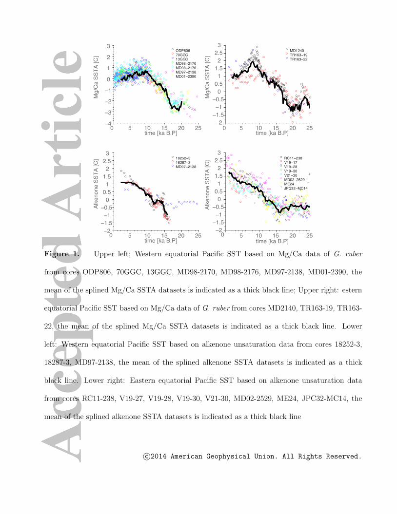
Whereas alkenone-based SSTs in the eastern and western equatorial Pacific indicate

continuous warming throughout the Holocene, with a magnitude similar to that of the

deglacial SST change, G. ruber Mg/Ca series usually indicate cooling from 8 ka B.P.

to present (see Fig. 1). Furthermore, alkenone-based deglacial warming in the eastern

equatorial Pacific starts around 16-15 ka B.P. (Fig. 1, lower right), in contrast to the much

earlier warming seen in the Mg/Ca SST data. In fact, the alkenone-derived warming starts

at a time when the Mg/Ca data have already attained about half of the glacial-interglacial

amplitude (Fig. 1, upper right panel). Understanding the causes for these discrepancies

will give us a deeper understanding of the controlling factors of Late Pleistocene and

Holocene climate change.

The key hypothesis that will be explored is that some first order discrepancies between

Mg/Ca and alkenone-based temperature proxies can be reconciled by invoking different

bulk seasonal sensitivities. Potential seasonal biases of SST proxy data have already been

discussed in previous studies (e.g. [Nurnberg et al., 2000; Ashkenazy and Tziperman, 2006;

Steinke and et al., 2008; Leduc et al., 2010; Schneider et al., 2010; Harada et al., 2012;


Wang et al., 2013; Rosell-Mele and Prahl, 2013]) by i.) identifying seasonal preferences

of coccolithphores and G. ruber in different regions and ii.) by comparing temperature

reconstructions with the orbital insolation trends that match the seasonal preferences of

the corresponding proxy [Leduc et al., 2010; Schneider et al., 2010].

Here we will further test this hypothesis by analysing satellite chlorophyll data, Uk′37,

sediment trap data, core top data and transient climate modeling experiments covering

the past 21 ka.

The paper is organized as follows. Following a critical assessment of the equatorial

Pacific SST proxy-data, seasonal and depth habitats of coccolithophores and G. ruber and

core-top alkenone/SST correlations (section 2), we will present a paleo-proxy data/model

comparison that is based on transient model solutions obtained with an earth system

model of intermediate complexity (section 3). The paper concludes with a summary and

discussion (section 4).

2. Proxy Data

To develop a better understanding of the discrepancies of Uk′37-SST and Mg/Ca-based

SST reconstructions on glacial/interglacial timescales we focus on a compilation of cores

from the western and eastern equatorial Pacific (see Tables 1,2), shown in Fig.1.

To highlight some of the common and most robust features in these records, we have

composited the alkenone (using 18252-3, 18287-3,MD97-2138 for the Western equato-

rial Pacific (WEP) and RC11-238, V19-27, V19-28, V19-30, V21-30,MD02-2529, ME24,

JPC32-MC14 for the Eastern equatorial Pacific (EEP)) (Fig. 1, lower panels, black lines)

as well as the Mg/Ca records (using ODP806, 70GGC, 13GGC, MD98-2170, MD98-2176,


MD97-2139, MD01-2390 for the WEP and MD1240, TR163-19, TR163-22 for the EEP)

(Fig. 1, upper panel, black lines) by linearly interpolating the proxy data in time and

averaging the resulting timeseries for the respective proxies and for the respective regions.

2.1. Seasonal biases due to spatial sampling

Before analysing the individual SST proxy records and comparing them to transient

climate model simulations, it is important to review the spatio- temporal structure of near

surface productivity and SSTs under present-day conditions. Here we use the SeaWifs

ocean-color derived chlorophyll [e.g. McClain et al., 1998; Yoder and Kennelly, 2003] as

a proxy for primary productivity. This data set is a monthly climatology obtained for

the period January 2003 to December 2006 and averaged on a 0.25 degree lat/lon grid

map. We compare the chlorophyll data to the SST climatology obtained from the AVHRR

satellite product averaged from January 1985 to December 2002 [Reynolds et al., 2007],

to evaluate the degree of spatial heterogeneity in productivity and SST by calculating

the month at which chlorophyll concentrations (SSTs) attain their maximum (minimum)

values. Fig. 2, upper panel reveals the high degree of spatial and seasonal complexity of

chlorophyll concentrations, and by extension, primary productivity. Large gradients for

instance in the north eastern tropical Pacific indicate that on scales of less than 1000 km

productivity can switch from a spring dominated regime to a fall dominated regime. It is

important to note that the month of coldest SST in the equatorial Pacific does not follow

the seasonal march of the sun across the equator. Eastern equatorial Pacific sites (Fig. 2)

both from the northern and southern hemisphere exhibit the lowest SST in boreal fall to

winter. The eastern equatorial Pacific data locations within 5◦ of the equator (see cyan


and red circles in Fig. 2 and Table 1), have a similar seasonal cycle in SST (Fig. 3,

upper right), irrespective of their positions north or south of the equator. In contrast, a

strong hemispheric gradient exists for chlorophyll concentrations in the eastern equatorial

Pacific (120◦W-90◦W). In other words, the season of maximum chlorophyll concentration,

and by extension, primary productivity, does not necessarily coincide with the season of

minimum SST. This is further exemplified in the western to central equatorial Pacific, east

of Papua New Guinea and in the South Pacific Convergence Zone area (Figs. 2,3). These

results challenge the use of SST climatologies as a simple proxy for surface productivity.

In our compilation of Uk′37 (Table 1) and Mg/Ca-based temperature reconstructions

(Table 2) seasonal biases may occur in a composite record (Fig. 1), if the majority of

the SST data came from regions with a productivity maximum in a particular season

and if productivity maxima were related to coccolithophore and foraminiferal abundances

and fluxes. The spatial inhomogeneity is further illustrated for our site locations in Fig.

2. We calculated the average of normalized satellite chlorophyll concentrations for all the

core locations in the eastern equatorial Pacific (lower right) and western equatorial Pacific

(lower left) with alkenone (red) and Mg/Ca (blue) records (see Tables 1,2 and Fig. 1,

circles). The alkenone data locations in the western equatorial Pacific are characterized

by strong boreal winter blooms (Fig. 3, lower left), corresponding to lower temperatures

(Fig. 3, upper left). A clear boral summer/fall preference can be found for the Mg/Ca

data locations in the eastern equatorial Pacific, consistent with lower SSTs (Fig. 2, upper

right). The situation for the Mg/Ca data locations in the western Pacific and the Uk′37

data in the eastern Pacific is less clear. In the former an early spring and late summer


peak dominate the chlorophyll signal, whereas in the latter we find only a weak seasonal

dependence in chlorophyll, in spite of a very pronounced seasonal cycle in SST.

This analysis demonstrated that the spatial heterogeneity of seasonal chlorophyll max-

ima, and by extension, productivity maxima, may further complicate the attribution of

seasonal biases of aggregated (spatially-combined) alkenone and Mg/Ca temperature re-

constructions.

2.2. Proxy-dependent seasonal biases

A more detailed view of potential seasonal biases of Mg/Ca and alkenone-based tem-

perature reconstructions at single locations has been obtained from sediment trap stud-

ies. Fig. 4 shows the fluxes of G. ruber in the Panama basin (upper left) [Thunell and

Reynolds, 1984] and the satellite-derived chlorophyll concentrations at the sediment trap

site (lower left). Although chlorophyll concentrations, and inferred primary productivity,

peak in boreal spring, the largest flux of G. ruber is observed in boreal summer. A lag in

the population of zooplankton grazers (e.g., foraminifera) relative to primary producers

(e.g., coccolithophorids) is commonly observed in the ocean, as is a lag in the sinking

flux of plankton relative to the standing stock, so this is not surprising. The situation for

Mg/Ca in the Western equatorial Pacific, namely in the South China Sea is a little bit

more difficult to interpret. Whereas Tian et al. [2005] report maximum fluxes of G. ruber

that peak on average from December to March during the season of maximum chlorophyll

concentrations, another South China Sea sediment trap about 600 km away documents

peak productivities in April and October [Wan et al., 2010]. Whether such discrepan-


cies represent the patchiness of phytoplankton blooms or the large interannual monsoon

variability is still an open question.

A better correspondence is found between the abundance of coccolithophores (Fig. 4,

upper) and chlorophyll concentrations (lower right) in the South China Sea [Chen et al.,

2007]. A very strong boreal winter peak in both suggests that Uk′37-based temperature

reconstructions, at least in the vicinity of the sediment trap, are likely to exhibit a winter

bias. Other studies in the tropical Pacific [Brown and Yoder, 1994; Wiesner et al., 1996;

Ziveri and Thunell, 2000; Harada et al., 2001] also discuss a possible boreal winter pref-

erence for alkenone-producing coccolithophorids. It has to be noted here, that alkenone

fluxes have been observed to peak during El Nino events in the Baja California Sur re-

gion [Hernandez-Becerril et al., 2007; Silverberg et al., 2004], which may be interpreted

to indicate a potential bias towards warm conditions. However, El Nino situations are

very different from just an enhanced annual cycle, as they can be accompanied by major

changes of thermocline depth, upwelling and nutrient regimes. Moreover, with El Nino

conditions peaking preferentially during boreal winter [Stein et al., 2011], any inferred

seasonal bias from this observation may be regarded as ambiguous.

Taken together, the studies discussed above further motivate the possibility for a strong

seasonal modulation in regional coccolithophore abundances in the equatorial Pacific.

This also suggests that the water temperatures, captured by the alkenone unsaturation

index are likely to be seasonally weighted, as hypothesized in numerous other studies.


2.3. Correlation of core-top alkenone data with SST

Many paleo-proxy studies [e.g. Muller et al., 1998; Rosell-Mele et al., 2004; Kienast

et al., 2012; Conte et al., 2006] have used the assumption that a high spatial correlation

between core-top Uk′37 values and the annual mean SST implies that alkenone data actually

represent annual mean SSTs. Using a recent compilation of 123 EEP alkenone core top

data [Kienast et al., 2012] and a present-day longterm SST climatology [Reynolds et al.,

2002] sampled at the core locations, we test the statistical stringency of this inference. Fig.

5, upper panel shows the pattern correlation between monthly mean climatological SST

and the alkenone-based SST reconstructions. We find values of > 0.79 for all months,

indicating that the overall SST pattern, except for an offset, remains relatively stable

during the course of the year. Highest values, exceeding even the correlation with annual

mean SST, are found for the month of June.

In order to compare the correlations amongst each other and determine statistically sig-

nificant differences we first transform the correlation values into Fisher’s Z-score. There-

after, the Z-scores are compared following Cohen and Cohen [1983] to obtain a corre-

sponding two-tailed p-value. The specific null-hypothesis we are testing is ”The pattern

correlation between core top alkenone-based SSTs and annual mean SST equals the cor-

relation between core top Uk′37-based SSTs and longterm monthly mean SST”. The results

of this hypothesis testing are shown in Fig. 5, lower panel. We find that we can re-

ject the null hypothesis with high confidence (> 90% ) for the months of February and

March. However, for all other months, the correlation coefficient is statistically indis-

tinguishable from the annual mean correlation. It should be noted here that the lower


alkenone/SST core top correlations during February and March seem to be at odds with

the idea of higher coccolithophore abundances in some equatorial Pacific locations [e.g.

Harada et al., 2001; Chen et al., 2007], such as the western tropical Pacific (see e.g. Fig.

4). A more in-depth analysis of this mismatch would have to take into account the fact

that sedimentation rates in the eastern equatorial Pacific are very low (∼ 2 cm/ka), and

that alkenone core-top data may represent averages over hundreds to thousands of years,

rather than the just the present-day conditions.

This suggests that from a statistical point of view alkenone-based SST in the EEP could

be interpreted as representing annual mean SST, or any other month (except February

and March), or combinations thereof. Thus, the high correlation between alkenone-derived

core top SSTs and observed annual mean SST is not a sufficient criterion for an annual

mean interpretation of alkenone data.

Another issue worth noting here is that a high spatial correlation between two different

fields (e.g. alkenone and annual mean SST) does not necessarily imply a high temporal

correlation between alkenone and annual mean SSTs, unless the spatial mean state pattern

of SST is similar to the leading patterns of variability on the timescale under consideration.

2.4. Orbital-scale variations of alkenone SSTs in the equatorial Pacific

Returning now to the averaged Uk′37-based SST indices in the EEP (Fig.1, lower right

panel), we find that the deglacial warming started around 16 ka B.P. which is ∼2 ka

after atmospheric CO2 concentrations began to rise from glacial to interglacial values

[Monnin et al., 2001; Luthi et al., 2008]. This warming continued monotonically into the

late Holocene. The Holocene trend of about 1◦-3◦C is comparable to the magnitude of


deglacial warming between 21-11 ka B.P. Similar features can be observed for the WEP

(Fig.1, lower left panel). The wide variety of depositional settings, including depth and

accumulation rate, surface and abyssal circulations, unique to each core and the fact that

the warming during Termination I (19-11 ka B.P.) and the Holocene are well reproduced

by the composites of alkenone data from cores in the EEP and WEP (thick back lines

in Fig. 1, lower panels) ensures that the signal is not the result of diagenesis or post-

depositional processes, such as bioturbation or sediment advection. While there is still

considerable scatter among the alkenone data from the EEP, all records show very similar

orbital-scale variations that track the composite index. This finding virtually excludes the

possibility that the longterm evolution in each core is determined by local processes such

as advection of alkenones on the seafloor or in surface currents. Possible explanations for

the quasi-monotonic warming trend in Uk′37 SST records across the equatorial Pacific during

the last 21 ka are (i) the mean annual temperature of surface waters throughout the equa-

torial Pacific increased, (ii) the season that the alkenone-producing coccolithophorids lived

warmed continuously, (iii) the alkenone producers gradually moved to shallower depths in

the water column, or (iv) the coccolithophorid season of growth became increasingly the

warm season throughout the Holocene at the expense of the cold season, or combinations

thereof. To address this question we will briefly review recent sediment trap studies.

The primary alkenone producers in the tropical Pacific are the coccolithophorids Emil-

iania huxleyi and Gephyrocapsa oceanica [Bentaleb et al., 2002; Ohkouchi et al., 1999;

Okada and Honjo, 1973]. As photoautotrophs the depth habitat of these and other coc-

colithophorids is presumed confined to the euphotic zone [Okada and Honjo, 1973]. Con-


sistent with that assumption Ohkouchi et al. [1999] re-analyzed the data of Okada and

Honjo [1973] and found that E. huxleyi and G. oceanica were most abundant between

0-100 m from 15◦N to 10◦S along the 155◦W meridian. This conclusion is consistent

with Bentaleb et al. [2002] who analyzed suspended particulate samples from the surface

mixed layer of the western tropical and subtropical Pacific Ocean. Fewer studies on the

depth habitat of coccolithophorids in the eastern equatorial Pacific exist but E. huxleyi is

thought to inhabit the upper euphotic zone there [Martinez et al., 2006]. Ohkouchi et al.

[1999] further found that core-top SST derived from alkenone unsaturation indices in the

central (155◦W) and western (175◦E) tropical Pacific tracked present-day surface annual

mean mixed layer temperatures reasonably well. However, as discussed in section 2.3 high

spatial correlations between core top Uk′37 data and annual mean mixed layer temperatures

do not necessarily imply that alkenone data represent annual mean conditions. In fact

Muller et al. [1998] report that seasonal correlations can be as high as annual mean cor-

relations, but different intercepts are to be expected in the regression and calibration of

proxy data and instrumental temperatures.

An approach that has been successfully applied to capture potential seasonal biases

in alkenone data is the production-weighted temperature [Sonzogni et al., 1997; Muller

et al., 1998; Schneider et al., 2010]. Using satellite-derived primary production rates and

assuming a high correlation between coccolithophorid production and total primary pro-

duction, the covariance between temperatures and primary production can be exploited

to develop a seasonal weighting of the alkenone data. This method has enabled a bet-


ter understanding of the discrepancies between alkenone and Mg/Ca-derived Holocene

temperature trends in terms of seasonality and orbital-scale forcings.

Inspired by the sediment trap studies discussed above, but also recognizing the potential

caveats of these sparse datasets, we propose the possibility that on average Uk′37-derived

SSTs in Late Pleistocene sediments from the equatorial Pacific may be biased towards

the winter season. While this is certainly not universally true, we will adopt this idea

as a working hypothesis to further test whether it may help to explain diverging trends

of alkenone-based SST and Mg/Ca based SST reconstructions. In our study we further

make the commonly applied assumption that the oceanographic and ecological processes

that promote these depth and seasonal growth patterns have remained roughly constant

throughout at least the last 21 ka so that sedimentary alkenones from the Last Glacial

Maximum (LGM) were likely to have been produced in the surface mixed layer in boreal

winter. We discuss the possibility for changes of this seasonal relationship in section 3.

2.5. Orbital-scale variations in G. ruber Mg/Ca-based SSTs in the equatorial

Pacific

While Uk′37-based SSTs increased across the equatorial Pacific through the Holocene,

SSTs derived from Mg/Ca ratios in the planktonic foraminifer G. ruber decreased.

Throughout the WEP (composite index in Fig. 1, upper left panel) and EEP (composite

index in Fig. 1, upper right panel ) G. ruber Mg/Ca SST records exhibit a considerable

Holocene cooling of 0.5-1.5◦C, starting around 9 ka B.P. There is also a clear indication for

an earlier onset of deglacial warming, in particular in the EEP, compared to the alkenone

record. The Mg/Ca SSTs also exhibit a stronger precessional signal in the sense that


maximum SSTs are attained around 9 ka and minimum SSTs around 20 ka B.P. The

discrepancies with the alkenone data, namely during the Holocene, are striking and call

for an explanation.

Holocene Mg/Ca trends could in principle also be generated by trends in calcium car-

bonate dissolution [Regenberg et al., 2014]. However, the high diversity of depositional

settings and water depths in 10 cores, exhibiting the Holocene Mg/Ca trends (Fig. 1,

upper panels) renders it highly unlikely that dissolution is the main cause [Brown and El-

derfield, 1996; Lea et al., 2000; Rosenthal and Lohmann, 2002; Rosenthal et al., 2000]. The

one exception would be if equatorial Pacific waters from 1-4 km became more corrosive

to CaCO3 during the Holocene, such as would occur if the carbonate ion concentration of

the entire tropical Pacific Ocean below 1 km gradually and continuously decreased. Such

a scenario cannot be ruled out entirely because a substantial decrease in the carbonate ion

concentration of the deep (> 3 km) equatorial Pacific has been inferred from planktonic

foraminiferal shell weights since the LGM [Broecker and Clark, 2001] with an estimated 8

mol/kg decline in [CO2−3 ] occurring in the Holocene at depths below 3 km [Broecker et al.,

1999]. In the 1-3 km depth range, however, these studies report no evidence for a car-

bonate ion decline of this magnitude during the Holocene. Barring a dissolution-derived

cooling artefact the Holocene cooling trend implied by G. ruber Mg/Ca is assumed real

and could be explained by (i) a decrease in the mean annual temperature of surface waters

throughout the equatorial Pacific, (ii) cooling during the season that G. ruber grows, (iii) a

gradual deepening of the depth habitat of G. ruber, or (iv) the growing season of G. ruber

became increasingly the cold season throughout the Holocene at the expense of the warm


season. This latter explanation would complicate the interpretation of Mg/Ca-derived

temperature tremendously.

To further explore possibility ii), we briefly review recent sediment trap studies. The

depth habitat of G. ruber is generally assumed to be the euphotic zone since it is host to

photoautotrophic symbionts. This is borne out by net tow studies in the western equatorial

Pacific [Lin and Hsieh, 2007] and the eastern equatorial Pacific [Fairbanks et al., 1982].

The season of maximum G. ruber abundance in the western equatorial Pacific is boreal

summer [Kawahata et al., 2002; Lin et al., 2004; Tian et al., 2005; Troelstra and Kroon,

1989; Wiesner et al., 1996]. G. ruber also reach maximum abundances in boreal summer

in the eastern tropical Pacific, as indicated by the sediment trap study by Thunell and

Reynolds [1984] using data from the Panama Basin (Fig. 4, left panel). In the Baja

California region G. ruber abundances in the stratified surface mixed layer also tend

to peak during the summer/fall [McConnell and Thunell, 2005; Wejnert et al., 2010].

Whereas, there may be site-specific regional differences, with respect to when exactly G.

ruber abundances peak, we infer that there appears to be a general tendency for a G.

ruber summer maximum in the tropical Pacific. This would translate also into a summer

bias of calcification temperatures.

2.6. Discussion of seasonal sensitivities in proxy data

Our analysis above has critically assessed various lines of reasoning to suggest that

EEP/WEP alkenone and Mg/Ca SST reconstructions could be seasonally biased. How-

ever, the exact determination of the seasonal biases for our proxy locations (Fig. 2)

remains inconclusive. For instance, spatial inhomogeneities in the seasonal production


of phytoplankton (Fig. 2) can complicate the situation. Furthermore, with only very

few longterm tropical Pacific sediment trap records available (Fig. 4) it is very difficult

to translate their results to other regions in the equatorial Pacific. Another conundrum

arises from the fact that EEP alkenone core top data show a relatively weak correlation

(Fig. 3) with boreal winter SST, in spite of recent findings from tropical oceans suggesting

potential boreal winter biases in the production of alkenone-producing coccolithophores.

Given these uncertainties, it becomes apparent that a different approach is needed to

reconcile the diverging trends in alkenone and Mg/Ca-based SSTs in the EEP and WEP

(Fig. 1). Rather than relying on sparse observational present-day datasets, we will exploit

the physical climate responses to the well-known external forcings during the last 21 ka

using a 3-dimensional climate model. By comparing the spatially averaged paleo-SST

reconstructions in Fig. 1 with simulated seasonal temperatures and by focusing on the

onset of seasonally-modulated deglacial warming and Holocene trends, we will be able to

deduce potential seasonal biases in the EEP and WEP alkenone and Mg/Ca SST datasets.

3. Model-proxy data comparisons over the last 21 ka

. Next we use a model of intermediate complexity to evaluate the hypothesis that the

differing trends in SST derived from alkenones and Mg/Ca can be attributed to insolation-

driven changes in the summer and winter seasons in the equatorial Pacific. Previous

studies have focused on Holocene temperature trends and used time-slice experiments

conducted with CGCMs [Schneider et al., 2010] or transient coupled model simulations

forced only by orbital insolation variations [Lorenz et al., 2006; Lohmann et al., 2013].

To estimate the effect of time-varying greenhouse gases, ice-sheets and orbital insolation


variations on the surface temperature evolution in the equatorial Pacific, we use the earth

system model of intermediate complexity LOVECLIM in a series of transient climate

simulations covering the last 21 ka.

3.1. Model Description

The atmospheric component of the coupled model LOVECLIM is ECBilt [Opsteegh

et al., 1998], a spectral T21, three-level model, based on quasi-geostrophic equations

extended by estimates of the neglected ageostrophic terms in order to close the equations

at the equator. The model contains a full hydrological cycle which is closed over land by

a bucket model for soil moisture. Synoptic variability associated with weather patterns is

explicitly computed. Diabatic heating due to radiative fluxes, the release of latent heat

and the exchange of sensible heat with the surface are parameterized and a prescribed

present-day cloud climatology is used. The sea ice-ocean component of LOVECLIM, CLIO

[Goosse et al., 1999; Goosse and Fichefet, 1999; Campin and Goosse, 1999] consists of a

free-surface primitive equation model with 3◦x3◦ resolution coupled to a thermodynamic-

dynamic sea ice model.

Coupling between atmosphere and ocean is done via freshwater and heat fluxes, rather

than by virtual salt fluxes. To avoid a singularity at the North Pole the oceanic component

makes use of two subgrids: The first one is based on classic longitude and latitude coordi-

nates and covers the whole ocean except the North Atlantic and Arctic ocean. These are

covered by the second spherical subgrid, which is rotated and has its poles at the equator

in the Pacific (1110 West) and Indian Ocean (690 east). The coupled model also uses

a very weak freshwater flux correction, which represents a moisture transport from the


North Atlantic to the North Pacific. For our purposes here the effect of this freshwater

flux correction can be neglected.

This LOVECLIM model and its former version ECBilt-Clio have been used extensively

in previous transient paleo climate modeling studies (e.g. Renssen et al. [2005]; Goosse

et al. [2006]; Timm and Timmermann [2007]; Timm et al. [2007]; Timmermann et al.

[2009]; Timm et al. [2010]; Menviel et al. [2011]).

3.2. External-Forcing

To quantify the effects of orbital forcing and other time-varying boundary conditions

on the evolution of seasonal temperatures, we present the solutions from three transient

model experiments. Experiment TR-21 (described in Timm and Timmermann [2007])

uses time-varying atmospheric CO2, CH4 and N2O concentrations for the last 21 ka,

following greenhouse gas measurements from the EPICA DOME C ice core [Spahni et al.,

2005; Luthi et al., 2008]. Orbitally-induced variations in the daily mean irradiance are

calculated following Berger [1978]. The ice-sheet forcing in this experiment uses 1000-year-

long slabs provided by the Peltier [1994] paleotopography reconstructions. The effect of

ice-sheets is felt by the atmosphere through changes in topography, albedo and changing

vegetation coverage. This experiment does not employ orbital acceleration (see Timm

and Timmermann [2007] and it was initialized from an equilibrated coupled Last Glacial

Maximum (LGM) simulation.

Experiment ORB (described in Timmermann et al. [2009]) only uses time-varying

orbital forcing, keeping greenhouse gas and ice-sheet forcing at LGM values. This model

simulation that started from an equilibrated LGM state was accelerated by a factor of


10 to save computing time. Hence the 21 ka forcing history is compressed into a 2,100-

year long simulation. As demonstrated in Timm and Timmermann [2007], an acceleration

factor of 10 is not expected to influence equatorial SST dynamics greatly. This experiment

will provide an estimate of the effects of orbital forcing only on equatorial SST during the

last 21 ka.

We also analysed a 3 member ensemble of transient orbitally-forced simulations con-

ducted with the ECHO-G coupled general circulation model. More details on this ex-

periment can be found in Lorenz and Lohmann [2004], Felis et al. [2004], Lorenz et al.

[2006], Timmermann et al. [2007] and Uchikawa et al. [2010]. Under pre-industrial CO2

concentrations, the ECHO-G experiment uses accelerated orbital forcing and an accel-

eration factor of 100. The model starts with the orbital configuration corresponding to

the year 142 ka B.P. and ends in the year 22.9 ka after present. We calculated the mean

of the simulated seasonal temperatures averaged over 3 ensemble members and focus

only on the period 21 ka B.P. - 0 ka B.P. From the LOVECLIM and ECHO-G experi-

ments we extracted fixed-length seasonal mean surface temperatures area-averaged over

the northeastern (6◦S-6◦N and 260-280◦E) and northwestern equatorial Pacific (10◦S-10◦N

and 105-160◦E ).

3.3. Model-paleo-proxy data comparison and inferences on seasonal biases

Fig. 6 shows the simulated late boreal summer (July, August, September mean) and

winter (December-January-February mean) temperatures in the eastern and western equa-

torial Pacific from TR-21, in comparison with the stacked Mg/Ca and alkenone SST

records from Fig. 1. Both seasons were chosen to yield an optimal match between model


simulation and proxy data. We observe a good qualitative match between model and

proxy data. In both the western and eastern equatorial Pacific there is a tendency for

the simulated temperatures to peak around 10 ka, with a slowly decreasing trend into

the Late Holocene. It is only during summer and fall that a decreasing temperature

trend during the Holocene is simulated in TR-21 (Fig. 6). The onset of the deglacial

warming is well captured by the simulated summer temperatures, although the model

simulations do not invoke millennial-scale forcings such as freshwater pulses related to

Heinrich event 1 and the Younger Dryas. It is important to note the amplitude of the

simulated deglacial July/August/September (JAS) temperature trends is underestimated

by a factor of 2-3 compared to the Mg/Ca SST reconstructions. This is likely due to

the fact that LOVECLIM exhibits a relatively strong atmospheric damping to equato-

rial SST anomalies. The simulated December/January/February (DJF) temperatures in

the eastern and western equatorial Pacific track the continuous reconstructed alkenone

temperature trend throughout the Holocene as well as the onset of the deglacial warming

around 16 ka B.P.. In the western equatorial Pacific the simulated amplitude of the overall

warming trend is underestimated, whereas it is well reproduced in the eastern equatorial

Pacific. These results suggest that a seasonal interpretation of Mg/Ca and alkenone data

may help reconciling their divergent behavior during the Holocene and the last glacial

termination.

To further disentangle the seasonal climate evolution in the eastern equatorial Pacific

in terms of orbital and other forcings, we study the simulated temperature history in

experiment ORB (Fig. 7). The DJF temperature evolution exhibits a precession signal,


which contributes by about 1◦C to the Holocene trend, seen in the alkenone proxy data.

The temperature trend in DJF in TR-21 is governed to first order by the CO2 forced

signal, and the orbital effect with some contributions from the decreasing Laurentide ice-

sheet height on equatorial Pacific SST, as discussed in Timmermann et al. [2004] using

an earlier version of LOVECLIM. The origin of delayed deglacial DJF warming starting

around 16 ka B.P. can be traced back to the fact that during the period 20-16 ka B.P.

the CO2 and icesheet forcings are still relatively weak and the temperature evolution is

largely controlled by the orbitally-induced cooling trend in SON.

Note also that, in contrast to the considerations of Leduc et al. [2010], the DJF insolation

signal is not in-phase with the DJF temperature evolution (see Fig. 7, dark grey lines).

This can be explained by the fact that the mixed layer temperature evolution due to

orbitally-induced changes of the shortwave radiation is to first order governed by

T (t) =

∫ t

0

Qinc(t)(1− α)

cpρHmix

e−λ(t−t′) dt′, (1)

where α corresponds to the long term mean regional albedo in the eastern equatorial Pa-

cific (cloud-albedo feedbacks are ignored for simplicity) and Qinc(t) denotes the orbitally-

induced variations in top-of-the atmosphere solar insolation (i.e. the orbitally-modulated

annual cycle forcing). cp is the heat capacity of water and ρ the density of seawater. The

average mixed layer depth is denoted as Hmix. The damping rate λ partly controls the

delay between forcing and response. In the eastern equatorial Pacific with a mean mixed

layer depth of Hmix=30 m and λ−1 ∼ 3− 4months [Barnett et al., 1991], the annual cycle

forcing Q(t) and its modulation through the Milankovitch cycles translates into a tem-

perature response that lags the forcing by about 2 months [Laepple and Lohmann, 2009].


In other words the DJF (MAM, JJA, SON) temperatures in ORB will be determined

by OND (JFM, AMJ, JAS) seasonal insolation changes associated with the precessional

cycle.

The March/April/May (MAM) SST trend in ORB (Fig. 7, upper right) features a

precessional-scale cooling from 20-8 ka B.P. and a subsequent warming that contributes to

the mid-to-late Holocene warming induced by the other time-varying boundary conditions,

namely the orbital insolation changes during January/February/March (JFM). The boreal

summer season June/July/August (JJA) (Fig. 7, lower left) is marked by a temperature

maximum around 11-12 ka B.P. and a subsequent cooling trend that continues until 5 ka

B.P. The JJA SST variations in ORB are a result of the seasonally averaged insolation

variations during April/May/June (AMJ). An early warming occurs during JJA as a result

of increasing insolation during AMJ. Clearly the seasonal interpretation of the alkenone

and Mg/Ca SSTs, capturing different phases of the precessional cycle, can help to explain

the different onsets in deglacial warming in Fig. 1. The September/October/November

(SON) boreal fall temperature evolution in TR-21 is a combination of greenhouse gas, ice-

sheet forcing and a precessional cycle that peaks around 9 ka B.P. According to equation

(1) and assuming a damping timescale λ−1 of 2-3 months we conclude that the late summer

orbital forcing is mainly responsible for the SON temperature variations.

Comparison of the simulated northeastern equatorial Pacific SSTs in ORB with an

orbitally-forced run (Fig. 6, cyan lines) that was performed with the ECHO-G coupled

general circulation model (Lorenz and Lohmann [2004]; Felis et al. [2004]; Lorenz et al.

[2006]; Timmermann et al. [2007] and Uchikawa et al. [2010]) suggests that the tropical


SST sensitivity to orbital forcing is similar in LOVECLIM to the more realistic ECHO-G

model.

These idealized modeling results suggest that the seasonal SST evolution in the equato-

rial Pacific can be interpreted as a lagged response to the seasonally varying orbital forc-

ing anomalies, greenhouse gas variations and ice-sheet forcing. The response of equatorial

SSTs to just greenhouse gas and the ice-sheet forcing is relatively constant throughout the

year (not shown). Hence, to explain the different behavior of Uk′37-based and Mg/Ca-based

SST, orbital forcing from different seasons has to be invoked.

3.4. Combining seasonal model and proxy data

Rather than discarding one SST proxy over another, our study suggests that they

provide complementary information that can be further exploited to estimate annual

mean temperatures, as well as the strength of the seasonal cycle in SST. This approach

is demonstrated in Fig. 8. In fact, using the transient climate model experiment TR-21,

we can test how well the annual mean temperature variations in the EEP (Fig.8, upper

panel, blue line, behind red line) can be reconstructed by just using the mean of boreal

summer and boreal winter temperatures (Fig.8, upper panel, red line). The resulting

timeseries are virtually identical. Furthermore, we can calculate the difference between

simulated boreal summer and boreal winter temperatures as a proxy for the strength

of the seasonal cycle in SST. The resulting timeseries (Fig. 8, upper panel, cyan line)

exhibits a clear precessional cycle with a maximum peaking around 12-13 ka B.P. and is

virtually identical to the strength of the seasonal cycle (not shown). Inspired by these

results and the proposed seasonal interpretation of Mg/Ca, Uk′37 data, we calculate the


average and difference of Mg/Ca SST anomalies and alkenone SST anomalies (Fig. 8,

lower panel). The average SST of alkenone and SST is quite similar to the simulated

annual mean temperature (Fig.8, upper panel, blue line). The difference between Mg/Ca

and alkenone-based SSTs (Fig. 8, lower panel, cyan line) shows similar characteristics to

the model simulated annual cycle strength, except for a relatively long plateau between

14-10 ka B.P.

From this analysis we observe that annual mean EEP SST variations, derived from

the combination of alkenone and Mg/Ca SST composites appear to be strongly linked

to the CO2 radiative forcing. The overall glacial/amplitude attains values of up to 2◦C,

which is lower than estimates of annual mean SST differences (∼2◦C) from the WEP

[Tachikawa et al., 2014] (their Fig. S1 based on cores MD05-2920, MD98-2161, ODP806

B, MD06-2067, MD01-2378, MD97-2140). This suggests a possible weakening of the

zonal SST gradient for glacial conditions. Whether glacial/interglacial CO2 changes are

the controlling factor for this reduction is uncertain, given the presence of other potential

contributors to EEP SST changes associated with for instance ice-sheet-driven changes of

the subtropical cells [Timmermann et al., 2004].

4. Summary and Discussion

We have attempted to explain why alkenone and Mg/Ca - derived SST reconstructions

in the equatorial Pacific often diverge from one another during the last 21 kyr. In par-

ticular, alkenone records across the equatorial Pacific indicate a warming trend during

the Holocene, while Mg/Ca records indicate cooling. By using a model of intermediate

complexity driven by insolation, greenhouse gases and ice sheets we are able to show that


these divergent trends could be explained by differing seasons of growth, with alkenone

production in the boreal winter and G. ruber production during boreal summer. This

timing of growth is consistent with low latitude Pacific sediment trap studies [Brown and

Yoder, 1994; Wiesner et al., 1996; Chen et al., 2007; Ziveri and Thunell, 2000; Harada

et al., 2001]. However, these primarily model-based conclusions need to be interpreted

with caution, given the spatial inhomogeneity of seasonal phytoplankton production rates

discussed in section 2. Moreover, the inferred seasonal biases for spatially averaged east-

ern and western equatorial Pacific alkenone and Mg/Ca SST reconstructions are by no

means universal and should not be applied to other regions.

Previous sediment trap studies suggest that on average G. ruber abundances in the trop-

ical Pacific peak in boreal summer. Late summer temperatures (average of July, August,

September) simulated by a transient 21 ka simulation conducted with the LOVECLIM

earth system model reproduce some key features of the Mg/Ca SST data compilation

such as the Holocene cooling trend and the onset of deglacial warming around 17-18 ka

B.P. Due to a 2 month lag between annual insolation and SSTs in the equatorial Pacific,

we conclude that Mg/Ca SSTs, at least during the last 21 ka, were driven by early sum-

mer insolation changes, in combination with other forcings that act year-round such as

greenhouse gas forcing and the remote effect of the glacial ice-sheets on the atmospheric

circulation. Other factors that may contribute to the evolution of Mg/Ca temperatures

include salinity variations [e.g. Hertzberg and Schmidt, 2013; Honisch et al., 2013] that

are affected by changes in global ice-volume as well as changes in the position of the In-

tertropical Convergence Zones. This aspect of the Mg/Ca-temperature calibrations has


not been thoroughly discussed in our study, but is likely to complicate the interpretation

of Mg/Ca-based temperature signals in the tropical Pacific.

According to sediment trap data in the tropical Pacific [e.g. Harada et al., 2001; Chen

et al., 2007], coccolithophorid blooms are likely to occur during winter months. In fact,

the simulated winter temperatures in the equatorial Pacific match the alkenone recon-

structions qualitatively (and in the EEP also quantitatively) well. The increasing late

fall-early winter insolation trend during the Holocene, in combination with increasing

CO2 concentrations leads to a near-monotonic increase in alkenone temperatures. The

somewhat delayed deglacial warming can be attributed to the fact that the late fall to

early winter insolation drops from the LGM into the early Holocene which compensates

for some of the CO2-induced winter temperature changes between 19-16 ka B.P. The effect

of millennial-scale variability on the timing of deglacial temperature changes in the EEP

is further discussed in Dubois et al. [2014]. A word of caution is necessary here. It should

be noted that the although the model-derived boreal winter alkenone interpretation for

the aggregated equatorial Pacific cores proposed here is consistent with several tropical

Pacific sediment core studies [Brown and Yoder, 1994; Wiesner et al., 1996; Chen et al.,

2007; Ziveri and Thunell, 2000; Harada et al., 2001], it seems inconsistent with the results

of our statistical EEP core-top analysis, which in fact identifies the months of February

and March, as those with the lowest spatial correlation with the core-top data. Further-

more, we found high spatial heterogeneity in seasonal chlorophyll concentrations (Fig. 2).

If this was also true for the corresponding fluxes of coccolithophores this ”patchiness”

may further limit the application of our conclusions to individual sites.


While acknowledging some important model/proxy data mismatches, we propose that

based on our model analysis, the most parsimonious explanation for divergent trends

in equatorial Pacific SST inferred from alkenones and G. ruber Mg/Ca would be that

alkenone producers and G. ruber live in different seasons in the tropical Pacific and that

orbital precession-driven changes in insolation could help reconcile the divergent behavior

of alkenone and Mg/Ca SSTs in the equatorial Pacific. This interpretation would offer

the potential of combining Uk′37 and Mg/Ca data of G. ruber from different cores to ob-

tain information on seasonality and annual mean conditions. We recommend that future

efforts to extract information on EEP climate from sediment cores should exploit this

unique opportunity, rather than focus just on one of the proxies.

Acknowledgments

The authors would like to thank Drs. Tom Koutavas, Guillaume Leduc, Nathalie Dubois

and Markus Kienast for providing their datasets from the tropical Pacific and for insightful

discussions. We are also grateful to Dr. Stephan Lorenz for making the ECHO-G transient

runs available to us. Support for this research came in part from grants NSF-OCE-0624954

(J.S.) and NOAA-NA06OAR4310122 (J.S.). A.T. acknowledges funding from NSF grant

No. 1010869. Additional support was provided by the Japan Agency for Marine-Earth

Science and Technology (JAMSTEC), through their sponsorship of research activities at

the International Pacific Research Center. Data presented in this paper will be shared

upon request.


References

Ashkenzy, Y., Tziperman, E., 2006. Scenarios regarding the lead of equatorial

sea surface temperature over global ice volume. Paleoceanography 21, PA 2006,

doi:10.1029/2005PA001232.

Barnett, T., Latif, M., Kirk, E., Roeckner, E., 1991. On ENSO physics. J. Clim. 4,

487–515.

Bentaleb, I., Fontugne, M., Beaufort, L., 2002. Long-chain alkenones and Uk’37 variabil-

ity along a south-north transect in the Western Pacific Ocean. Global and Planetary

Change 34, 173–183.

Berger, A. L., 1978. Long-term variations of daily insolation and Quaternary climatic

changes 35 (12), 2362–2367.

Broecker, W., Clark, E., 2001. Glacial-to-Holocene Redistribution of Carbonate Ion in

the Deep Sea. . Science 294, 2152–2155.

Broecker, W., Clark, E., McCorkle, D., Peng, T.-H., Hajdas, I., Bonani, G., 1999.

Evidence for a reduction in the carbonate ion content of the deep sea during the

course of the Holocene. . Paleoceanography 14, 744–752.

Brown, C., Yoder, J., 1994. Coccolithophorid blooms in the global ocean. . Journal of

Geophysical Research 99(C4), 7467–7482.

Brown, S., Elderfield, H., 1996. Variations in Mg/Ca and Sr/Ca Ratios of Plank-

tonic Foraminifera Caused by Postdepositional Dissolution: Evidence of Shallow Mg-

Dependent Dissolution. . Paleoceanography 11, 543–551.


Campin, J., Goosse, H., 1999. A parameterization of dense overflow in large-scale ocean

models in z coordinate. Tellus 51A, 412–430.

Chen, Y.-L., Chen, H.-Y., Chung, C.-W., 2007. Seasonal variability of coccolithophore

abundance and assemblage in the northern South China Sea. . Deep Sea Research

Part II: Topical Studies in Oceanography 54(14-15), 1617–1633.

Cohen, J., Cohen, P., 1983. Applied multiple regression/correlation analysis for the

behavioral sciences. Oxford, England: Lawrence Erlbaum.

Conte, M., Sicre, M.-A., Ruhlemann, C., Weber, J. C., Schulte, S., Schulz-Bull, D.,

Blanz, T., 2006. Global temperatur calibration of the alkenone unsaturation indx UK′37

in surface waters and comparison with surface sediments . Geochemistry, Geophysics,

Geosystems, 7, Q2005, doi:10.1029/2005GC001054.

de Garidel-Thoron, T., Rosenthal, Y., Beaufort, L., Bard, E., Sonzogni, C., Mix, A.,

2007. A multiproxy assessment of the western equatorial pacific hydrography during

the last 30 kyr. Paleoceanography 22, PA3204, doi:10.1029/2006PA001269.

Dubois, N., Kienast, M., Kienast, S., Timmermann, A., 2014. Millennial-scale At-

lantic/East Pacific sea surface temperature linkages during the last 100,000 years.

Earth Planetary Science Lett., 396, 134-142.

Fairbanks, R., Sverdlove, M., Free, R., Wiebe, P., Be, A., 1982. Vertical Distribution

and Isotopic Fractionation of Living Planktonic Foraminifera from the Panama Basin.

. Nature 298, 841–844.

Felis, T., Lohmann, G., Kuhnert, H., Lorenz, S., Scholz, D., Patzold, J., Rousan, A. A.,

Al-Moghrabi, S., 2004. Increased seasonality in Middle East temperatures during the


last interglacial period. Nature 429, 164–168.

Fraile, O., Schulz, M., Mulitza, S., Merkel, U., Prange, M., Paul, A., 2009. Modeling

the seasonal distribution of planktonic foraminifera during the last glacial maximum.

Paleoceanography 24, PA2216, doi:10.1029/2008PA001686.

Goosse, H., Arzel, O., J, L., Mann, M. E., Renssen, H., Riedwyl, N., Timmermann, A.,

Xoplaki, E., Wanner, H., 2006. The Origin of the ”European Medieval Warm Period”.

Climate of the Past 2, 99–113.

Goosse, H., Deleersnijder, E., Fichefet, T., England, M., 1999. Sensitivity of a global

coupled ocean-sea ice model to the parameterization of vertical mixing. J. Geophys.

Res. 104(C6), 13681–13695.

Goosse, H., Fichefet, T., 1999. Importance of ice-ocean interactions for the global ocean

circulation: a model study. J. Geophys. Res. 104(C10), 23337–23355.

Harada, N., Handa, N., Harada, K., Matsuoka, H., 2001. Alkenones and particulate

fluxes in sediment traps from the central equatorial Pacific. Deep-Sea Res. Pt I 48,

891–907.

Harada, N., Sato, M., Nakamura, Y., Kimoto, K., Okazaki, Y., Nagashima, K., Gor-

barenko, S. A., Seki, O., Moossen, H., Bendle, J., Ijiri, A., Nakatsuka, T., Menviel,

L., Chikamoto, M. O., Timmermann, A., Abe-Ouchi, A., 2012. Sea surface and sub-

surface temperature changes in the okhotsk sea and adjacent north pacific during the

last glacial maximum and deglaciation. Deep Sea Research II, 61-64, 93–105.

Hernandez-Becerril, D., BravoSierra, E., Ake-Castillo, J., 2007. Phytoplankton on the

western coasts of Baja California in two different seasons in 1998. Scientia Marina 71,


doi:10.3989/scimar.2007.71n4735.

Hertzberg, J.E., Schmidt, M.W., 2013. Refining Globigerinoides ruber Mg/Ca pale-

othermometry in the Atlantic Ocean. Earth and Planetary Science Letters, 383, 123–

133

Honisch, B., Allen, K.A., Lea, D.W., Spero, H.J., Eggin, S.M., Arbuszewski, J,m de-

Menocal, P., Rosenthal, Y., Russell, A.D., Elderfield, H., 2013. The influence of salin-

ity on Mg/Ca in planktic foraminifers Evidence from cultures, core-top sediments

and complementary δ18O . Geochimica et Cosmochimica Acta 121, 196213.

Kawahata, H., Nishimura, A., Gagan, M., 2002). Seasonal change in foraminiferal pro-

duction in the western equatorial Pacific warm pool: evidence from sediment trap

experiments. . Deep Sea Research Part II: Topical Studies in Oceanography 49(13-

14), 2783–2800.

Kienast, M., MacIntyre, G., Dubois, Higginson, S., Normandeau, C., Chazen, C., Her-

bert, T. D., 2012. Alkenone unsaturation in surface sediments from the eastern equa-

torial Pacific: Implications for SST reconstructions. Paleoceanography 27, PA1210,

doi:10.1029/2011PA002254.

Kienast, M., Steinke, S., Stattegger, K., Calvert, S., 2001. Synchronous tropical south

china sea sst change and greenland warming during deglaciation. Science 291, 2132–

2134.

Kienast, S., Kienast, M., Jaccard, S., Calvert, E., Francois, R., 2006. Testing the

silica leakage hypothesis with sedimentary opal records from the eastern equa-

torial pacific over the last 150 kyrs. Geophysical Research Letters 33, L15607,


doi:10.1029/2006GL026651.

Koutavas, A., Jr, J. L.-S. T. M., Sachs, J., 2002. El Nino-Like Pattern in Ice Age

Tropical Pacific Sea Surface Temperature. . Science 297(5579), 226–230.

Koutavas, A., Sachs, J., 2008. Northern timing of deglaciation in the eastern

equatorial Pacific from alkenone paleothermometry. Paleoceanography 23, PA4205,

doi:10.1029/2008PA001593.

Laepple, T., Lohmann, G., 2009 The seasonal cycle as template for climate variability on

astronomical time scales. Paleoceanography, 24, PA4201, doi:10.1029/2008PA001674

Lea, D., Pak, D., Belanger, C., Spero, H., Hall, M., Shackleton, N., 2006. Paleoclimate

history of galapagos surface waters over the last 135,000 yrs. Quaternary Science

Reviews 25, 1152–1167.

Lea, D., Pak, D., Spero., H., 2000. Climate impact of late quaternary equatorial pacific

sea surface temperature variations. Science 289, 1719–1724.

Leduc, G., Schneider, R., Kim, J. H., Lohmann, G., 2010. Holocene and Eemian sea

surface temperature trends as revealed by alkenone and Mg/Ca paleothermometry.

Quaternary Science Reviews 29, 989–1004.

Leduc, G., Vidal, L., Tachikawa, K., Rostek, F., Sonzogni, C., Beaufort, L., Bard, E.,

2007. Moisture transport across Central America as a positive feedback on abrupt

climatic changes. . Nature 445(7130), 908–911.

Lin, H., Hsieh, H.-Y., 2007. Seasonal variations of modern planktonic foraminifera in

the South China Sea. . Deep Sea Research Part II: Topical Studies in Oceanography

54(14-15), 1634–1644.


Lin, H., Wang, W.-C., Hung, G.-W., 2004. Seasonal variation of planktonic foraminiferal

isotopic composition from sediment traps in the South China Sea. . Marine Micropa-

leontology 53(3-4), 447–460.

Linsley, B., Rosenthal, Y., Oppo., D., 2010. Holocene evolution of the indonesian

throughflow and the western pacific warm pool. Nature Geoscience 3, 578–583.

Lohmann, G., Pfeiffer, M., Laepple, T., Leduc, G., and Kim, J.-H 2013: A model-data

comparison of the Holocene global sea surface temperature evolution. Clim. Past, 9,

1807–1839, doi:10.5194/cp-9-1807-2013

Lorenz, S., Kim, J.-H., Rimbu, N., Schneider, R., Lohmann, G., 2006. Orbitally driven

insolation forcing on Holocene climate trends: Evidence from alkenone data and cli-

mate modeling. Paleoceangraphy 21, PA1002, doi:10.129/2005PA001152.

Lorenz, S., Lohmann, G., 2004. Acceleration technique for Milankovitch type forcing

in a coupled atmosphere-ocean circulation model: method and application for the

Holocene. Clim. Dyn. 23, 727–743, doi:10.1007/s00382-004-0469.

Luthi, D., Floch, M. L., Bereiter, B., Blunier, T., Barnola, J.-M., Siegenthaler, U.,

Raynaud, D., Jouzel, J., Fischer, H., Kawamura, K., Stocker, T., 2008. High-resolution

carbon dioxide concentration record 650,000-800,000 years before present. Nature 453,

379–382.

Martinez, I., Rincon, D., Yokoyama, Y., Barrows, T., 2006. Foraminifera and coc-

colithophorid assemblage changes in the Panama Basin during the last deglaciation:

Response to sea-surface productivity induced by a transient climate change. . Palaeo-

geography, Palaeoclimatology, Palaeoecology 234(1), 114–126.


McClain, C., Cleave, M., Feldman, G., Gregg, W., Hooker, S., Kuring, N., 1998. Science

quality SeaWiFS data for global biosphere research. Sea Technology 39, 10–16.

McConnell, M., Thunell, R., 2005. Calibration of the planktonic foraminiferal Mg/Ca

paleothermometer: Sediment traps results from the Guaymas Basin. Paleoceanogra-

phy 20, PA2016, doi:10.1029/2004PA001077.

Medina-Elizalde, M., Lea, D., 2005. The mid-pleistocene transition in the tropical pa-

cific. Science 310, 1009–1012.

Menviel, L., Timmermann, A., Timm, O. E., Mouchet, A., 2011. Deconstructing the

Last Glacial termination: the role of millennial and orbital-scale forcings. Quaternary

Science Reviews, 30, 1155–1172.

Monnin, E., Indermuhle, A., Dallenbach, A., Fluckiger, J., Stauffer, B., Stocker, T. F.,

Raynaud, D., Barnola, J.-M., 2001. Atmospheric CO2 concentrations over the last

glacial termination. Science 291, 112–114.

Muller, P., Kirst, G., Ruhland, G., von Storch, I., Rosell-Mele, A., 1998. Calibration

of the alkenone paleotemperature index UK′37 based on core-tops from the eastern

south atlantic and the global ocean (60◦n-60◦s). Geochimica et Cosmochimica Acta

62, 1757–1772.

Nurnberg, D., Muller, A., Schneider, R. R., 2000. Paleo-sea surface temperature cal-

culations in the equatorial east Atlantic from Mg/Ca ratios in planktic foraminifera:

A comparison to sea surface temperature estimates from UK′37 , oxygen isotopes, and

foraminiferal transfer function . Paleoceanography 15, 124–134.


Ohkouchi, N., Kawamura, K., Kawahata, H., Okada, H., 1999. Depth ranges of alkenone

production in the central Pacific Ocean . Global Biogeochemical Cycles 13, 695–704.

Okada, H., Honjo, S., 1973. The distribution of ocanic coccolithophorids in the Pacific

. Deep-Sea Research 20, 355–374.

Opsteegh, J., Haarsma, R., Selten, F., Kattenberg, A., 1998. ECBILT: A dynamic

alternative to mixed boundary conditions in ocean models. Tellus 50A, 348–367.

Pahnke, K., Sachs, J., Keigwin, L., Timmermann, A., Xie, S.-P., 2007. Eastern tropical

pacific hydrologic changes during the past 27,000 years from d/h ratios in alkenones.

Paleoceanography 22, PA4214, doi:10.1029/2007PA001468.

Peltier, W. R., 1994. Ice age paleotopography. Science 265, 195–201.

Pena, L., Cacho, I., Ferretti, P., Hall, M., 2008. El ninosouthern oscillationlike variability

during glacial terminations and interlatitudinal teleconnections. Paleoceanography 23,

PA3101, doi:10.129/2008PA001620.

Regenberg, M., Regenberg, A., Garbe-Schonberg, A., Lea, D.W., 2014. Global

dissolution effects on planktonic foraminiferal Mg/Ca ratios controlled by the

calcite-saturation state of bottom waters, Paleoceanography, 29, 127-142, doi:

10.1002/2013PA002492

Renssen, H., Goosse, H., Fichefet, T., 2005. Contrasting trends in North Atlantic deep-

water formation in the Labrador Sea and Nordic Seas during the Holocene. Geophys.

Res. Lett. 32, L08711, doi:10.1029/2005GL022462.

Reynolds, R., Rayner, N., Smith, T., Stokes, D., Wang, W., 2002. An improved in situ

and satellite SST analysis for climate. J. Clim. 15, 1609–1625.


Reynolds, R., Smith, T., Liu, C., Chelton, D. B., Casey, K. S., Schlax, M. G., 2007. Daily

High-Resolution-Blended analyses for sea surface temperature. J. Clim. 20, 5473–5496.

Rosell-Mele, A., Bard, E., Grieger, B., Hewitt, C., Muller, P., Schneider, R., 2004.

Sea surface temperature anomalies in the oceans at the LGM estimated from the

alkenone-UKk′37 index: comparison with GCMs. Geophys. Res. Lett. 39, L03208,

doi:10.1029/2003GL018151.

Rosell-Mele, A. and Prahl, F.G. 2013. Seasonality of UK’37 temperature estimates

as inferred from sediment trap data. Quaternary Science Reviews. 72 128136,

10.1016/j.quascirev.2013.04.017

Rosenthal, Y., Lohmann, G., 2002. Accurate estimation of sea surface temperatures

using dissolution-corrected calibrations for Mg/Ca paleothermometry. Paleoceanogra-

phy 17, doi:10.1029/2001PA000749.

Rosenthal, Y., Lohmann, G., Lohmann, K., Sherrell, R., 2000. Incorporation and

Preservation of Mg in Globigerinoides sacculifer: Implications for Reconstructing the

Temperature and 18O/16O of Seawater. Paleoceanography 15(1), 135–145.

Schneider, B., Leduc, G., Park, W., 2010. Disentangling seasonal signals in

holocene climate trends by satellite-proxy integration. Paleoceanography 25, PA4217,

doi:10.120/2009PA001893.

Silverberg, N., Martinez, A., niga, S. A., Carriquiry, J., Romero, N., Shumilin, E., Cota,

S., 2004. Contrasts in sedimentation flux below the southern California Current in late

1996 and during the El Nino event of 19971998. Estuarine, Coastal and Shelf Science

59, 575–587.


Sonzogni, C., Bard, E., Rostek, F., Lafont, R., Rosell-Mele, A., Eglinton, G., 1997.

Core-top calibration of the alkenone index vs sea surface temperature in the Indian

Ocean. Deep Sea Res. II 44, 1445–1460.

Spahni et al., R., 2005. Atmospheric methane and nitrous oxide of the late Pleistocene

from Antarctic ice cores. Science 310, 1317–1321.

Stein, K., Timmermann, A., Schneider, N., 2011. Phase synchronization of the El Nino-

Southern Oscillation with the annual cycle. Phys. Rev. Lett., 107(12), 128501 .

Steinke, S., et al., 2008. Proxy dependence of the temporal pattern of deglacial warming

in the tropical south china sea: Toward resolving seasonality. Quat. Sci. Rev. 27,

688–700.

Stott, L., et al., 2004. Decline of sea surface temperature and salinity in the western

tropical pacific ocean during the holocene epoch. Nature 431, 56–59.

Stott, L., Timmermann, A., Thunell, R., 2007. Southern Hemisphere and Deep-Sea

Warming Led Deglacial Atmospheric CO2 Rise and Tropical Warming. Science 318,

435–438.

Tachikawa, K., Timmermann, A., Vidal, L., Sonzogni, C., Elison Timm, O., 2014: CO2

radiative forcing and Intertropical Convergence Zone influences on western Pacific

warm pool climate over the past 400 ka, Quaternary Science Reviews, 86, 15 24–34.

Thunell, R., Reynolds, L., 1984. Sedimentation of Planktonic Foraminifera: Seasonal

Changes in Species Flux in the Panama Basin. . Micropaleontology 30(3), 243–262.

Tian, J., Wang, P., Chen, R., Cheng, X., 2005. Quaternary upper ocean thermal gradient

variations in the South China Sea: implications for east Asian monsoon climate.


Paleoceanography, 20, doi:10.1029/2004PA001115.

Timm, O., Kohler, P., Timmermann, A., Menviel, L., 2010. Mechanisms for the onset

of the African Humid Period. J. Clim., 23(10), 2612–2633.

Timm, O., Timmermann, A., 2007. Simulation of the last 21,000 years using accelerated

transient boundary conditions. J. Climate 20, 4377–4401.

Timm, O., Timmermann, A., Abe-Ouchi, A., Segawa, T., 2007. On the defini-

tion of paleo-seasons in transient climate simulations. Paleoceanography, PA2221,

doi:10.1029/2007PA001461.

Timmermann, A., Justino, F., Jin, F.-F., Krebs, U., Goosse, H., 2004. Surface tempera-

ture control in the North and tropical Pacific during the last glacial maximum. Clim.

Dyn. 23, 353–370.

Timmermann, A., Lorenz, S., An, S.-I., Clement, A., Xie, S.-P., 2007. The Effect of

Orbital Forcing on the Mean Climate and Variability of the Tropical Pacific. J. Clim.

20, 4147–4159.

Timmermann, A., Timm, O., Menviel, L., 2009. The roles of CO2 and orbital forcing

in driving southern hemispheric temperature variations during the last 21,000 years.

J. Climate 22, 1626–1640.

Troelstra, S., Kroon, D., 1989. Note on extant planktonic Foraminifera from the Banda

Sea, Indonesia (Snellius-II Expedition, cruise G5). Netherlands . Journal of Sea Re-

search 24, 459–463.

Uchikawa, J., Popp, B., Schoonmaker, J., Timmermann, A., Lorenz, S., 2010. Geo-

chemical and climate modeling evidence for Holocene aridification in Hawaii: dynamic


response to a weakening equatorial cold tongue. Quat. Sci. Rev. 29, 3057–3066.

Wan, S., Jian, Z., Cheng, X. R., Qiao, P. J., Wang, R. J., 2010. Seasonal variations in

planktonic foraminiferal flux and the chemical properties of their shells in the southern

South China Sea. Science China, Earth Sciences 53, 1176–1187.

Wang, Y.V., Leduc,G., Regenberg, G., Andersen N., Larsen, T.,Blanz, T., Schneider, R.

R. 2013. Northern and southern hemisphere controls on seasonal sea surface tempera-

tures in the Indian Ocean during the last deglaciation. Paleoceanography, 28, 619632,

doi:10.1002/palo.20053

Wejnert, K., Pride, C., Thunell, R., 2010. The oxygen isotope composition of plank-

tonic foraminifera from the Guaymas Basin, Gulf of California: Seasonal, annual, and

interspecies variability. Marine Micropaleontology 74, 29–37.

Wiesner, M., andH.K. Wong, L. Z., Wang, Y., Chen, W., 1996. Fluxes of particulate

matter in the South China Sea. In: V. Ittekot, P. Schafer, S. Honjo, P.J. Depetris

(Eds.), Particle Flux in the Ocean . (Ed. by V. Ittekot, P. Schafer, S. Honjo, P.J.

Depetris), pp. 293–312. Wiley, New York.

Yoder, J., Kennelly, M., 2003. Seasonal and ENSO variability in global ocean phyto-

plankton chlorophyll derived from 4 years of SeaWiFS measurements. Global Biogeo-

chemical Cycles 17, 1112, doi:10.1029/2002GB001942.

Ziveri, P., Thunell, R., 2000. Coccolithophore export production in Guaymas Basin,

Gulf of California: response to climate forcing. . Deep Sea Research Part II: Topical

Studies in Oceanography 47(9-11), 2073–2100.


Table 1. Alkenone SST reconstructions used in this study

Proxy Core Location Depth (m) Reference

Alkenone MD97-2138 1.25◦S, 146.15◦E 1960 de Garidel-Thoron et al. [2007]Alkenone 18252-3 9.23◦N 109.4◦W 1273 Kienast et al. [2001]Alkenone 18287-3 5.7◦N 110.7◦E 598 Kienast et al. [2001]Alkenone RC11-238 1.5◦S 85.5◦W 2573 Koutavas and Sachs [2008]Alkenone V19-27 0.28◦S 82.1◦W 1373 Koutavas and Sachs [2008]Alkenone V19-28 2.4◦S 84.65◦W 2720 Koutavas and Sachs [2008]Alkenone V19-30 3.4◦S 83.5◦W 3091 Koutavas and Sachs [2008]Alkenone V21-30 1.2◦S 89.7◦W 617 Koutavas and Sachs [2008]Alkenone MD02-2529 8.2◦N 84.1◦W 1619 Leduc et al. [2007]Alkenone ME0005A-24JC 1.5◦N 86.5◦W 2941 Kienast et al. [2006]Alkenone MC14 4.8◦N 77.6◦W 884 Pahnke et al. [2007]Alkenone JPC32 4.6◦N 77.9◦W 2200 Pahnke et al. [2007]Alkenone ME0005-27JC 1.8◦S 82.8◦W 2203 Kienast et al. [2006]Alkenone TR163-19P 2.2◦N 91◦W 2348 Kienast et al. [2006]


Table 2. Mg/Ca SST reconstructions used in this study

Proxy Core Location Depth Reference

Mg/Ca G. ruber TR163-19 2.2◦N 91◦W 2348 Lea et al. [2000]Mg/Ca G. ruber ODP806 0.3◦N 159◦E 2520 Medina-Elizalde and Lea [2005]Mg/Ca G. ruber TR163-22 0.5◦N 92.3◦W 2830 Lea et al. [2006]Mg/Ca G. ruber 70GGC 3.55◦S 119.3◦E 482 Linsley et al. [2010]Mg/Ca G. ruber 13GGC 7.45◦S 115.2◦E 2924 Linsley et al. [2010]Mg/Ca G. ruber MD98-2170 GGC 10.6◦S 125.4◦E 832 Stott et al. [2007]Mg/Ca G. ruber MD98-2176 5◦S 133.3◦E 2382 Stott and et al. [2004]Mg/Ca G. ruber MD97-2138 1.25◦N 146.1◦E 1960 de Garidel-Thoron et al. [2007]Mg/Ca G. ruber MD01-2390 6.6◦N 113.5◦E 1545 Steinke and et al. [2008]Mg/Ca G. ruber ODP 1240 0◦N 86.5◦W 2921 Pena et al. [2008]


0 5 10 15 20 25−4

−3

−2

−1

0

1

2

3

time [ka B.P]

Mg/

Ca

SS

TA

[C]

ODP80670GGC13GGCMD98−2170MD98−2176MD97−2138MD01−2390

0 5 10 15 20 25−2

−1.5−1

−0.50

0.51

1.52

2.53

time [ka B.P]

Mg/

Ca

SS

TA

[C]

MD1240TR163−19TR163−22

0 5 10 15 20 25−2

−1.5−1

−0.50

0.51

1.52

2.53

time [ka B.P]

Alk

enon

e S

ST

A [C

]

18252−318287−3MD97−2138

0 5 10 15 20 25−2

−1.5−1

−0.50

0.51

1.52

2.53

time [ka B.P]

Alk

enon

e S

ST

A [C

]

RC11−238V19−17V19−28V19−30V21−30MD02−2529ME24JPC32−MC14

Figure 1. Upper left; Western equatorial Pacific SST based on Mg/Ca data of G. ruber

from cores ODP806, 70GGC, 13GGC, MD98-2170, MD98-2176, MD97-2138, MD01-2390, the

mean of the splined Mg/Ca SSTA datasets is indicated as a thick black line; Upper right: estern

equatorial Pacific SST based on Mg/Ca data of G. ruber from cores MD2140, TR163-19, TR163-

22, the mean of the splined Mg/Ca SSTA datasets is indicated as a thick black line. Lower

left: Western equatorial Pacific SST based on alkenone unsaturation data from cores 18252-3,

18287-3, MD97-2138, the mean of the splined alkenone SSTA datasets is indicated as a thick

black line. Lower right: Eastern equatorial Pacific SST based on alkenone unsaturation data

from cores RC11-238, V19-27, V19-28, V19-30, V21-30, MD02-2529, ME24, JPC32-MC14, the

mean of the splined alkenone SSTA datasets is indicated as a thick black line


Figure 2. Upper panel: Month of maximum chlorophyll concentration from the SEAWIFS

ocean color satellite climatology [McClain et al., 1998; Yoder and Kennelly, 2003]. Lower panel:

Month of minimum SST obtained from the AVHRR satellite SST climatology. Cyan (red) circles

indicate core locations of alkenone (Mg/Ca) SST reconstructions.


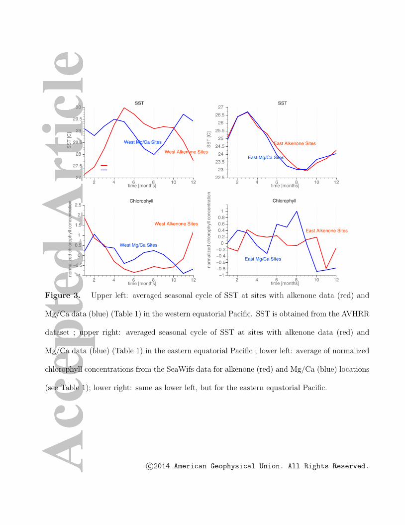
2 4 6 8 10 1227

27.5

28

28.5

29

29.5

30

time [months]

SS

T [C

]

SST

West Alkenone Sites

West Mg/Ca Sites

2 4 6 8 10 1222.5

23

23.5

24

24.5

25

25.5

26

26.5

27

time [months]

SS

T [C

]

SST

2 4 6 8 10 12−1

−0.5

0

0.5

1

1.5

2

2.5

time [months]

norm

aliz

ed c

hlor

ophy

ll co

ncen

trat

ion Chlorophyll

2 4 6 8 10 12−1

−0.8−0.6−0.4−0.2

00.20.40.60.8

1

time [months]

norm

aliz

ed c

hlor

ophy

ll co

ncen

trat

ion

Chlorophyll

East Mg/Ca Sites

East Alkenone Sites

West Mg/Ca Sites

West Alkenone Sites

East Alkenone Sites

East Mg/Ca Sites

Figure 3. Upper left: averaged seasonal cycle of SST at sites with alkenone data (red) and

Mg/Ca data (blue) (Table 1) in the western equatorial Pacific. SST is obtained from the AVHRR

dataset ; upper right: averaged seasonal cycle of SST at sites with alkenone data (red) and

Mg/Ca data (blue) (Table 1) in the eastern equatorial Pacific ; lower left: average of normalized

chlorophyll concentrations from the SeaWifs data for alkenone (red) and Mg/Ca (blue) locations

(see Table 1); lower right: same as lower left, but for the eastern equatorial Pacific.


Dec Jan Feb Mar Apr May Jun Jul Aug Sep Oct Nov0

100

200

300

400

Spe

cim

ens

G. r

uber

< 5

00 m

icro

met

er /m

^2/d

ay

Eastern Pacific

Winter Spring Summer Fall0

20

40

60

80

Coc

cosp

here

den

sity

[x 1

0^3/

l]

South China Sea

Dec Jan Feb Mar Apr May Jun Jul Aug Sep Oct Nov0.2

0.3

0.4

0.5

0.6

0.7

Chl

orop

hyll

Pan

ama

Winter Spring Summer Fall0.1

0.15

0.2

0.25

0.3

0.35C

hlor

ophy

ll S

CS

Coccolithophore abundanceG. ruber abundance

Figure 4. Upper left: Bi-monthly flux patterns for G. ruber in the Panama Basin, eastern

equatorial Pacific (Thunell and Reynolds, 1984), measured at about 900 m depth; Upper right:

Seasonal coccolithophorid fluxes in the South China Sea from Chen et al. (2007). The maximum

flux of coccolithophorids occurs in boreal winter. In addition, the alkenone-producing species E.

huxleyi and G. oceanica predominate the assemblage during that season (not shown); Lower left:

Mean climatological cycle of chlorophyll concentrations in the Panama Basin at the location of

the sediment trap of Thunell and Reynolds, 1984 derived from SeaWifs ocean color data; Lower

right: Mean climatological cycle of chlorophyll concentrations in the South China Sea.


0.7

0.75

0.8

0.85

0.9

2 4 6 8 10 12

Correlation between monthly SST and alkenone-based SST

0

20

40

60

80

100

2 4 6 8 10 12

Percentage level at which null hypothesis of equal correlation (ALK/monthly SST) (ALK/annual SST) can be rejected

ANNMMonth

95%90%

Corr

elat

ion

Reje

ctio

n le

vel o

f nul

l hyp

othe

sis

[%]

Month ANNM

Figure 5. Upper panel: Monthly spatial correlation between EEP core top alkenone values

from 123 sites [Kienast et al., 2012] and present-day climatological SST. Month 13 represents

the annual mean; Lower panel: Significance level (percent) at which the null hypothesis that a

monthly SST/alkenone correlation is statistically different from the annual mean SST/alkenone

correlation can be rejected. Results are based on Fisher’s Z-scores.


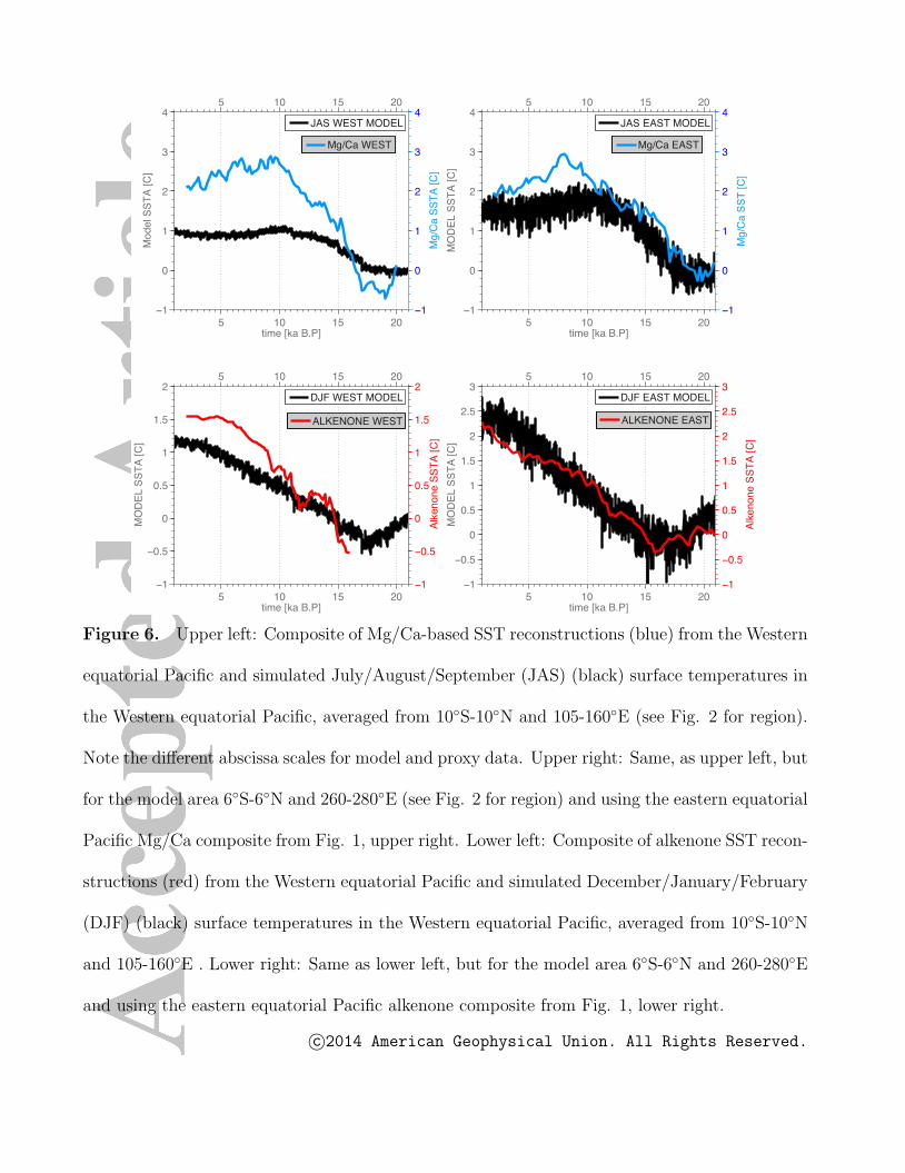
5 10 15 20−1

−0.5

0

0.5

1

1.5

2

time [ka B.P]

MO

DE

L S

ST

A [C

]

DJF WEST MODEL

5 10 15 20

−1

−0.5

0

0.5

1

1.5

2

Alk

enon

e S

ST

A [C

]

ALKENONE WEST

5 10 15 20−1

−0.5

0

0.5

1

1.5

2

2.5

3

time [ka B.P]

MO

DE

L S

ST

A [C

]

DJF EAST MODEL

5 10 15 20

−1

−0.5

0

0.5

1

1.5

2

2.5

3

Alk

enon

e S

ST

A [C

]

ALKENONE EAST

5 10 15 20−1

0

1

2

3

4

time [ka B.P]

Mod

el S

ST

A [C

]

JAS WEST MODEL

5 10 15 20

−1

0

1

2

3

4

Mg/

Ca

SS

TA

[C]

Mg/Ca WEST

5 10 15 20−1

0

1

2

3

4

time [ka B.P]

MO

DE

L S

ST

A [C

]

JAS EAST MODEL

5 10 15 20

−1

0

1

2

3

4

Mg/

Ca

SS

T [C

]

Mg/Ca EAST

Figure 6. Upper left: Composite of Mg/Ca-based SST reconstructions (blue) from the Western

equatorial Pacific and simulated July/August/September (JAS) (black) surface temperatures in

the Western equatorial Pacific, averaged from 10◦S-10◦N and 105-160◦E (see Fig. 2 for region).

Note the different abscissa scales for model and proxy data. Upper right: Same, as upper left, but

for the model area 6◦S-6◦N and 260-280◦E (see Fig. 2 for region) and using the eastern equatorial

Pacific Mg/Ca composite from Fig. 1, upper right. Lower left: Composite of alkenone SST recon-

structions (red) from the Western equatorial Pacific and simulated December/January/February

(DJF) (black) surface temperatures in the Western equatorial Pacific, averaged from 10◦S-10◦N

and 105-160◦E . Lower right: Same as lower left, but for the model area 6◦S-6◦N and 260-280◦E

and using the eastern equatorial Pacific alkenone composite from Fig. 1, lower right.


5 10 15 20

−1

−0.5

0

0.5

1

1.5

2

time [ka]

DJF

SS

T a

nom

aly

[K]

ALLORBORB ECHO−G

5 10 15 20

−20

−15

−10

−5

0

5

10

15

20

Inso

latio

n an

omal

y O

ND

[W/m

2 ]

5 10 15 20

−1

−0.5

0

0.5

1

1.5

2

time [ka]

MA

M S

ST

ano

mal

y [K

]

ALLORBORB ECHO−G

5 10 15 20

−20

−15

−10

−5

0

5

10

15

20

Inso

latio

n an

omal

y JF

M [W

/m2 ]

5 10 15 20

−1

−0.5

0

0.5

1

1.5

2

time [ka]

JJA

SS

T a

nom

aly

[K]

ALLORBORB ECHO−G

5 10 15 20

−20

−15

−10

−5

0

5

10

15

20

Inso

latio

n an

omal

y A

MJ

[W/m

2 ]

5 10 15 20

−1

−0.5

0

0.5

1

1.5

2

time [ka]

SO

N S

ST

ano

mal

y [K

]

ALLORBORB ECHO−G

5 10 15 20

−20

−15

−10

−5

0

5

10

15

20

Inso

latio

n an

omal

y JA

S [W

/m2 ]

Figure 7. Upper left Simulated DJF temperature anomalies in the Eastern equatorial Pacific

(average from 6◦S-6◦N and 260-280◦E, see Fig. 2 for region) for the transient simulations that

uses all forcings (red) TR-21 and a transient run that uses only orbital forcing ORB (blue),

whereas greenhouse gas and ice-sheet forcings are kept fixed at LGM values. The dark grey line

represents the near-equatorial orbital forcing anomalies 2 months prior to DJF. Upper right: same

as upper left, but for MAM. Lower left: same as upper left, but for JJA. Lower right: same as

upper left, but for SON. Note the 2-3 month delay between orbital forcing and the temperature

response in ORB. The cyan lines represent the respective 3-member ensemble mean seasonal

data of eastern equatorial Pacific SST, as simulated by the orbitally-forced transient ECHO-G

experiment (see Lorenz et al. [2006]; Timmermann et al. [2007]).


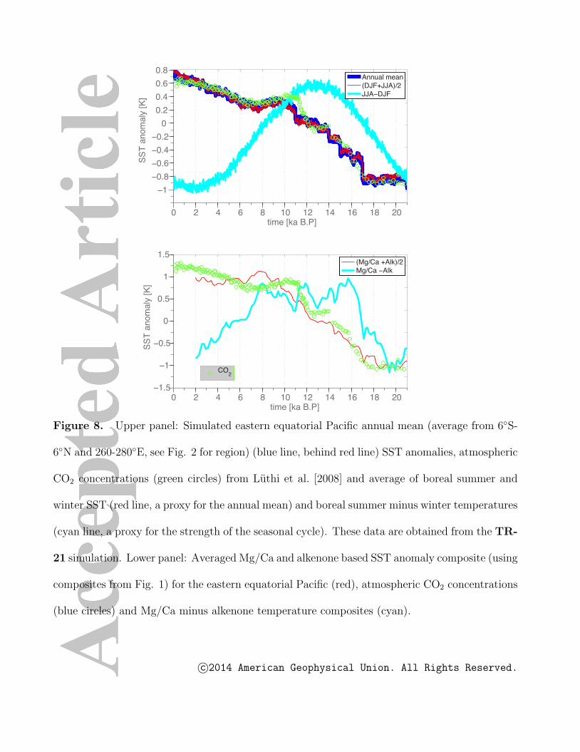
0 2 4 6 8 10 12 14 16 18 20

−1

−0.8

−0.6

−0.4

−0.2

0

0.2

0.4

0.6

0.8

time [ka B.P]

SS

T a

nom

aly

[K]

Annual mean(DJF+JJA)/2JJA−DJF

0 2 4 6 8 10 12 14 16 18 20−1.5

−1

−0.5

0

0.5

1

1.5

time [ka B.P]

SS

T a

nom

aly

[K]

(Mg/Ca +Alk)/2Mg/Ca −Alk

CO2

CO2

Figure 8. Upper panel: Simulated eastern equatorial Pacific annual mean (average from 6◦S-

6◦N and 260-280◦E, see Fig. 2 for region) (blue line, behind red line) SST anomalies, atmospheric

CO2 concentrations (green circles) from Luthi et al. [2008] and average of boreal summer and

winter SST (red line, a proxy for the annual mean) and boreal summer minus winter temperatures

(cyan line, a proxy for the strength of the seasonal cycle). These data are obtained from the TR-

21 simulation. Lower panel: Averaged Mg/Ca and alkenone based SST anomaly composite (using

composites from Fig. 1) for the eastern equatorial Pacific (red), atmospheric CO2 concentrations

(blue circles) and Mg/Ca minus alkenone temperature composites (cyan).


Assessing divergent SST behavior during the last 21 ka...

Documents

Transcript of Assessing divergent SST behavior during the last 21 ka...