Syracuse University Syracuse University

SURFACE SURFACE

Theses - ALL

August 2018

Assessing dissolved methane and halogen patterns in Assessing dissolved methane and halogen patterns in

groundwater of New York State groundwater of New York State

Shannon Garvin Syracuse University

Follow this and additional works at: https://surface.syr.edu/thesis

Part of the Physical Sciences and Mathematics Commons

Recommended Citation Recommended Citation Garvin, Shannon, "Assessing dissolved methane and halogen patterns in groundwater of New York State" (2018). Theses - ALL. 259. https://surface.syr.edu/thesis/259

This Thesis is brought to you for free and open access by SURFACE. It has been accepted for inclusion in Theses - ALL by an authorized administrator of SURFACE. For more information, please contact surface@syr.edu.

Abstract

Due to the ban on hydraulic fracturing for natural gas in New York State (NYS), it serves

as an ideal location to study the natural processes that control the migration of dissolved methane

and high salinity fluids found at depth. The hydrogeologic setting of NYS is analogous to that of

Northern Pennsylvania where unconventional exploration has not been restricted. Halogens

geochemically behave conservatively and can be found in unique proportions. Therefore, they

serve as useful tracers for the natural movement of groundwater. The focus of our study is to: 1)

establish a more cohesive baseline for groundwater quality data for NYS prior to the onset of

unconventional natural gas development than currently available; 2) evaluate the spatial variability

and hydrologic controls over dissolved methane, chloride, bromine, and iodine; and 3) further

evaluate the extent to which bromine-iodine mass ratios (Br/I) may be useful as a geochemical

tracer in groundwater in the Appalachian Basin.

Sampling occurred throughout the late summer and fall of 2016 and 2017. Water was

collected from domestic and public supply groundwater wells (n=108) located in five distinct

NYS hydrologic regions defined by major drainage basins: western NYS, central NYS, Broome

and Tioga Counties of southern NYS, the Mohawk River Basin, and the Upper Hudson River

Basin. The majority of samples (54%) had methane concentrations between 1-10 mg/L, 40% of

samples fell below the detection limit, and 6% of samples had methane greater than 10 mg/L, the

actionable level implemented by the US Department of the Interior Office of Surface Mining.

Mann-Whitney statistical tests on this dataset suggest that landscape position did not serve as a

strong control for elevated methane as suggested in previous studies. In contrast, the strongest

predictors for methane in potable groundwater appear to be: general bedrock type (i.e.

sedimentary or crystalline), height of the well bore above the Marcellus Shale, sodium (Na)-rich

water type, and degree of confinement. Halogen concentrations, particularly bromine and iodine,

can characterize saline formation waters naturally mixing with potable waters. The quality of

groundwater wells often consists of both shallow groundwater flow and some measure of Upper

and Middle Devonian (Marcellus Formation) waters from the bedrock below. Our results show

that iodine in conjunction with bromine can be utilized to identify the degree of formation water

influence in potable groundwater.

ASSESSING DISSOLVED METHANE AND HALOGEN PATTERNS IN GROUNDWATER

OF NEW YORK STATE

by

Shannon Renee Garvin

A.A.S., Onondaga Community College, 2012

B.S., State University of New York College at Cortland, 2015

Thesis

Submitted in partial fulfillment of the requirements for the degree of

Master of Science in Earth Sciences

Syracuse University

August 2018

Copyright © Shannon Renee Garvin 2018

All Rights Reserve

v

Acknowledgements

I am grateful to Syracuse University, The Department of Earth Sciences, and my advisor

Dr. Zunli Lu for taking me on as a graduate student. I want to thank my committee members Dr.

Don Siegel and Bill Kappel for their research guidance and expertise. Many thanks to the folks at

the United States Geological Survey in Ithaca and Troy, without whom I would not have had this

dataset. I would like to give a special thanks to my research group: Kristy Gutchess and Wanyi

Lu. I feel fortunate to have been mentored by two such outstanding scientists. I’d like to express

my appreciation to a few of the great professors: Dr. Laura Lautz for answering my spontaneous

questions, Dr. Christa Kelleher for being a great source of encouragement, and Dr. Daniel

Curewitz for your enthusiasm and passion for science teaching. Special thanks to Ben Fisher for

assisting me with his knowledge of GIS and for being supportive throughout this process. Most

importantly, I would like to thank my hardworking and selfless parents who instilled in me the

value of receiving a higher education at a young age and lived modestly so they could help me

do so. I am blessed to be surrounded by the people described above and could not have done this

without them. “I have learned that success is to be measured not so much by the position that one

has reached in life as by the obstacles which he has had to overcome while trying to succeed.”

- Booker T. Washington

vi

Table of Contents

Abstract ........................................................................................................................................... i

1. Introduction ............................................................................................................................... 1

1.1 Geologic History of the Appalachian Basin ......................................................................... 1

1.2 Utility of Halogens as a Tracer ............................................................................................. 2

1.3 Iodine Geochemistry ............................................................................................................. 3

1.4 Objectives ............................................................................................................................. 4

2. Location and Background ........................................................................................................ 4

2.1 Major Drainage Basins ......................................................................................................... 4

2.2 Geologic Background ........................................................................................................... 5

2.3. Hydrochemical Flow Systems ............................................................................................. 6

3. Methods ...................................................................................................................................... 6

3.1 Sampling Strategy and Protocol............................................................................................ 6

3.2 Analytical Methods ............................................................................................................... 8

3.3. Spatial Data Analysis ........................................................................................................... 9

3.4 Geochemical Methods ........................................................................................................ 10

3.5 Statistical Analysis of Data ................................................................................................. 11

4. Results ...................................................................................................................................... 11

5. Discussion ................................................................................................................................ 16

5.1 Controls on Groundwater Methane ..................................................................................... 16

5.1.1 Underlying Bedrock Geology .......................................................................................... 17

5.1.2 Topographic Position ....................................................................................................... 17

5.1.3 Water Type....................................................................................................................... 18

5.1.4 Confinement Conditions .................................................................................................. 19

5.1.5 Proximity to Existing Gas Wells...................................................................................... 20

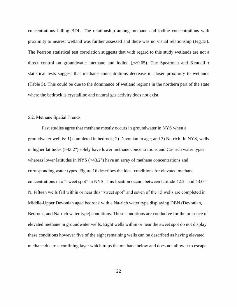
5.1.6 Proximity to Wetlands ..................................................................................................... 21

5.2. Methane Spatial Trends ..................................................................................................... 22

5.3 Major Water Chemistry and Mixing Endmembers ............................................................. 23

6. Summary and Conclusions .................................................................................................... 24

Tables ........................................................................................................................................... 26

Figures .......................................................................................................................................... 31

Appendix ...................................................................................................................................... 49

References .................................................................................................................................... 55

vii

List of Tables

Table 1: Characterization of sampling regions

Table 2: Geologic units for known bedrock wells

Table 3: Wells intersecting wetland soils with associated basin and water type

Table 4: Elevated iodine concentrations

Table 5: Statistical results of Pearson, Spearman, and Kendall correlation

viii

List of Figures

Figure 1: Map of study area

Figure 2: Conceptual groundwater diagram

Figure 3: Spatial distribution of methane and iodine concentrations

Figure 4: Relative frequency histograms

Figure 5: Map view of concentrations of bromine, iodine, and methane

Figure 6: Boxplots of topographic position

Figure 7: Boxplots of groundwater type

Figure 8: Piper diagram

Figure 9: Boxplots of completion material

Figure 10: Boxplots of methane concentrations in confinement analysis

Figure 11: Boxplots of iodine concentrations in confinement analysis

Figure 12: Proximity to “active” and “other” gas wells

Figure 13: Proximity to wetlands

Figure 14: Br/I ratios grouped by bedrock, methane, and latitude

Figure 15: Confinement conceptual diagram

Figure 16: Methane versus latitude

Figure 17: Br/I cross plot with known formation waters

1

1. Introduction

The extraction of natural gas by means of hydraulic fracturing in the northeastern United

States within the Appalachian basin has increased over the last fifteen years with improvements in

technology (Wen et al., 2018). The expansion of hydraulic fracturing has raised public concern for

the potential contamination of shallow aquifers used for drinking water (Osborn et al., 2011; Wen

et al., 2018). Hydraulic fracturing is currently banned in New York State (NYS), making it an

ideal location to study the natural processes that control the migration of dissolved methane and

associated high salinity fluids. Past studies have associated elevated methane concentrations in the

region with: 1) topographic position (Molofsky et al., 2013; Heisig & Scott, 2013; Wen et al.,

2018); 2) proximity to existing gas wells (Osborn et al., 2011; Jackson et al., 2013); and 3) a

sodium (Na)-rich groundwater type (McPhillips et al., 2014; Siegel et al., 2015; Christian et al.,

2016). Although the success on these controls on methane occurrence vary among each study.

1.1 Geologic History of the Appalachian Basin

The Appalachian Basin is an elongated foreland basin with an area of approximately

595,700 km2 having a length of 1,610 km and a width of 560 km which formed during the

Paleozoic era (Early Cambrian to Early Permian) (Colton, 1970; de Witt, 1993). The basin

contained a warm tropical sea that extended from present day New York to Alabama, favorable

conditions for the preservation of organic matter. Orogenic highlands northwest of the basin acted

as a major source for filling the basin with siliciclastic sediment (de Witt, 1993). A sequence of

carbonates, shales, siltstones, and sandstones are present throughout the Paleozoic formations and

2

show repeated sequences of sea level transgressions and regressions (Roen, 1984) and most of the

shales contain natural gas.

The Marcellus Shale and the Utica Shale (Fig.1) particularly contain sufficient natural gas

and in some places oil, to constitute major hydrocarbon plays in North America. The Devonian

aged Marcellus Shale of the Hamilton group bisects the entirety of the study area aside from the

Upper Hudson River Basin from east to west (Fig. 1). Many water wells in this area are drilled

into Devonian aged bedrock of the Marcellus Shale where it is shallow and not a viable gas source.

The much deeper Middle and Upper Ordovician aged Utica Shale underlies the Marcellus Shale

and is not as likely of an influence on much shallower groundwater wells. Hydraulic fracturing

and directional (horizontal) drilling has made extracting natural gas and oil from these low-

permeability shales accessible (Kappel and Nystrom, 2012).

1.2 Utility of Halogens as a Tracer

Halogen solutes (primarily chloride, bromine, and iodine) generally behave conservatively

in groundwater and occur in distinct proportions to one another in waters having different sources

of dissolved solids. Therefore, their ratios are useful for tracing the natural movement of

groundwater and for distinguishing sources of salinity ranging from road salt to septic effluent

(Davis et al., 1998; Panno et al., 2006; Lautz et al., 2014; Johnson et al., 2015; Gutchess et al.,

2016). In particular, chloride-bromide mass ratios (Cl/Br) prove to be effective to broadly

distinguish sources of salinity (Panno et al., 2006) but cannot distinguish between various

formation waters such as Marcellus Formation waters from older brines (Lu et al., 2014).

3

Therefore, another conservative solute needs to be examined, and to this end, iodine can serve the

purpose.

1.3 Iodine Geochemistry

Iodine is a biophillic element strongly enriched in marine organic matter, and therefore

accumulates in marine sediments (Elderfield and Truesdale, 1980; Fehn, 2012; Lu et al., 2014). In

groundwater, iodate and iodide are the main species of iodine (Li et al.,2017). Iodate is the primary

species in surface and shallow water having oxidizing conditions, with iodide being the primary

species in deeper (reducing) groundwater (Li et al., 2017). Weathering of organic-rich sedimentary

rocks of marine origin provides iodine to the terrestrial environment (Fehn, 2012; Lu et., 2014;

Alvarez, 2016). Iodine and methane are found in higher concentrations in sedimentary rocks

relative to crystalline and igneous rocks.

During the burial of organic matter, decomposition also produces methane which co-

releases with iodine into interstitial fluids (Lu et al., 2014). These fluids can escape to the surface

through natural fractures and faults and up into permeable unconsolidated materials, along drilled

well bores, or could remain trapped within the bedrock strata or below confining layers in

unconsolidated sediments. Freshwater mixing with formation waters will have a distinct Br/I ratio

that will differ from water that has come into contact with non-marine or organic-poor sedimentary

rocks (Lu et al., 2014). Iodine concentrations are elevated in the Appalachian Basin brines and

other oil and gas fields (Moran et al., 1995; Panno et al., 2006; Osborn et al., 2012; Lu et al., 2014).

This unique signature is used to explore how deeper Appalachian Basin fluids may mix with

shallower groundwater.

4

1.4 Objectives

The objectives of the study were to obtain groundwater quality data from both domestic

and public supply water wells from within Appalachian Basin in NYS in order to: 1) establish

baseline groundwater quality data for NYS; 2) examine distributions of dissolved methane, iodine,

bromine, and other solutes; 3) assess the hydrogeologic controls as they related to the occurrence

of iodine and methane in NYS groundwater; and 4) further explore the utility of the Br/I ratio as a

geochemical tracer in groundwater.

2. Location and Background

2.1 Major Drainage Basins

Fourteen major river basins are designated in NYS (excluding Long Island) as part of the

New York State Department of Environmental Conservation’s (NYSDEC) 305(b) program. This

study examined four regions across NYS in 2016 and 2017 as outlined by the 305(b) Project:

western New York (western NYS), the Mohawk River Basin (Mohawk RB), central New York

(central NYS), the Upper Hudson River Basin (Upper Hudson RB). Additional samples were

collected from Broome and Tioga County of south-central NYS (Broome and Tioga Co.) (Fig. 1).

Samples collected from Broome and Tioga County were part of the National Water Quality

Assessment Program (NAWQA). The data collected represent a subset of random samples from

across the majority of NYS.

5

2.2 Geologic Background

In general, bedrock in western NYS and central NYS including Broome and Tioga

Counties is sedimentary in origin and consist of interbedded shale, siltstone, sandstone, limestone,

and dolostone of Ordovician, Silurian, and Devonian age (Fisher et al., 1970; Table 1) which dip

southward and are overlain by till, with thicker layers of glacial till, lacustrine, and alluvial

sediment filling the glacially-carved valleys (Heisig and Scott, 2013). The river valleys are lined

with glacial material which compose the valley fill aquifers mapped by the USGS (Christian,

2015). The most common and productive aquifers in this area are the glaciofluvial deposits of sand

and gravel found within the valleys. Bedrock aquifers are used for water supply in the uplands

(Reddy, 2014).

The Mohawk RB in the eastern part of the state is composed predominately of sedimentary

bedrock with the northernmost wells within the basin being drilled in crystalline bedrock. The

bedrock of the Upper Hudson RB is largely composed of Cambrian and Ordovician aged

crystalline and sedimentary rocks that were deposited during the Taconic Orogeny (Isachsen et al.,

2000; Table 1). The bedrock of the northern portion of the basin is primarily crystalline

metamorphic rock comprised mostly of gneiss, and the southern portion of the basin is underlain

by metamorphosed clastic rocks (Scott and Nystrom, 2014; Christian, 2015). The dominant

bedrock type into which groundwater wells are drilled into in this study include the: Java-West

Falls Formation, Sonyea Group, Canadaway Group, and the Hamilton Formation (Table 2). The

dominant lithology for the Java-West Falls, Sonyea, and Canadaway Group is shale and siltstone

while within the Hamilton Formation the Marcellus Shale contains methane-bearing black shale

which is currently being explored for natural gas in northern Pennsylvania.

6

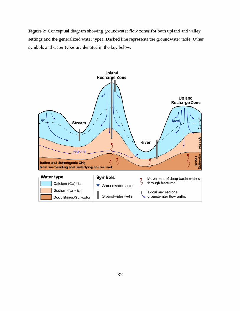
2.3. Hydrochemical Flow Systems

Hydrogeology of the study area includes fresh groundwater flow systems in the stratiform

sediment in the valleys and in fractured bedrock throughout the area. In freshwater systems,

Calcium (Ca)-rich water type overlies Sodium (Na)-rich connate saline water or brine (Williams,

2010; Heisig and Scott, 2013). The position of the freshwater/saltwater interface in both the valley

and upland areas is poorly defined due to limited data and uncertainties introduced by flow in

poorly-sealed wellbores. In valleys, the depth to saline water has been reported to be between 30

m to 100 m below the valley floor (Williams, 2010; Heisig and Scott, 2013). Groundwater flow in

a valley migrates from the valley walls toward the primary stream or river. This flow is most rapid

in shallow unconfined aquifers and most indolent in the deeper sand and gravel or bedrock aquifers

(Heisig and Scott, 2013). Figure 2 shows a generalized conceptual hydrochemical flow model for

the Appalachian Basin. Generally, older deeper groundwater becomes more mineralized due to

interactions with bedrock along lengthy flow paths and mixing with salt water or brines (Siegel et

al., 2015). These brines can contain thermogenic methane (Heisig and Scott, 2013) and iodine from

underlying and surrounding source rocks. Small streams can serve as local discharge zones,

whereas major river valleys can act as intermediate or regional groundwater discharge zones

(Siegel et al., 2015).

3. Methods

3.1 Sampling Strategy and Protocol

This project is the product of collaborative efforts between Syracuse University, the USGS

305(b) Ambient Groundwater Quality Project, and a regional NAWQA program. The 305(b)

7

Ambient Groundwater Quality Project is a cooperative project between the USGS and the NYS

Department of Environmental Conservation (NYSDEC) that satisfies the NYSDEC’s duties under

Section 305(b) the 1977 Amendments of the Federal Clean Water Act (Reddy, 2014). This law

requires that each state monitor and report on the chemical quality of both surface and groundwater

within the state's boundaries (U.S. Environmental Protection Agency, 1997). Groundwater wells

in each of the 14 major basins are sampled by the USGS on a rotational basis once every five years

and two or more of the 14 basins are sampled each year. Over 200 constituents were included in

the analysis as well as physical parameters, (e.g. temperature, pH, dissolved oxygen, etc.).

Approximately 50 wells were sampled each year from domestic and public supply wells. Domestic

wells were selected by using NYSDEC’s well water program

(http://www.dec.ny.gov/lands/4997.html). Groundwater samples were collected from the Mohawk

River Basin and western NYS in late 2016 and from the Upper Hudson River and the central NYS

basins in late 2017.

The 15 NAWQA groundwater samples were also collected in the fall of 2017 for a study

network which focused on wells near oil and gas drilling activities across the United States. In

Pennsylvania, where hydraulic fracturing is permitted, 15 domestic wells were sampled proximal

to gas wells, and 15 domestic wells were sampled distal to gas wells in an effort to assess if any

differences can be observed that could be attributed to drilling activities. The samples collected

from Broome and Tioga Counties in NYS, where drilling is not permitted, serve as a sub-network

of controls sites.

All samples were collected as close to the well as possible, typically at the pressure tank

and/or at an outdoor spigot prior to any form of water treatment. The well was purged until physical

8

parameters reached stability or until at least three well volumes had been removed from the well

casing. A flow cell, which is designed for groundwater sampling at low flow, was used to monitor

the stabilization of water quality parameters. To limit the potential for atmospheric contamination

of samples a sampling chamber, which is constructed of a PVC pipe frame and a sampling bin all

within a plastic bag enclosure, was constructed at each collection site.

Sample collection and preparation varied depending on the intended method of analysis.

Samples analyzed for major ions as well as bromine and iodine were filtered with a pre-rinsed 0.45

μM capsule filter and immediately placed in a cooler to be chilled at 4°C. Samples analyzed for

cations were preserved with nitric acid (HNO3). To sample for methane, a needle was inserted into

a rubber stopper until the tip exited through the stopper. A separate, larger beaker was then filled

with well water within the sampling chamber. The tubing connected to the spigot was placed at

the bottom of the 150 mL sample bottle located within the sampling chamber. After the sample

bottle was filled, it was fully submerged in the water-filled beaker with water continuously flowing

into the bottle. While the sample bottle was fully submerged, a rubber stopper with a hypodermic

needle was inserted into the sample bottle. The needle was extracted once the stopper was forced

into the top of the bottle to allow any extra water or gas bubbles to escape. The bottle was visually

examined to ensure that there were no bubbles adhering to the sides of the bottle. Duplicate

samples were collected at each well.

3.2 Analytical Methods

Samples were sent to various labs (including the USGS National Water Quality Lab

(NWQL) in Denver, CO; USGS Groundwater Age Dating Lab in Reston, VA; ALS-

9

Environmental Lab in Fort Collins, CO; and a local bacteria lab) for analysis of a multitude of

constituents including dissolved gasses. Halogen concentrations (total dissolved bromine and

iodine) for all samples were measured in the Syracuse University Department of Earth Sciences

Low Temperature Geochemistry Laboratory using a Bruker Daltronics Aurora M90 Quadrupole-

based inductively coupled plasma mass spectrometer (ICP-MS). Blanks were monitored every

three samples. Calibration standards were repeated every six samples. Instrument error for

concentrations of iodine and bromine measured on ICP-MS are typically less than 1%, thus are

not reported individually in this study. Detection limits for dissolved methane mg/L, bromine μg/L,

and iodine μg/L are: 0.001, 0.1, 0.01; respectively.

3.3. Spatial Data Analysis

ArcMap 10.4.1 was used for spatial analysis of the data. Two methods were used to

determine topographic position of each sampled well: 1) the National Hydrography Dataset (NHD)

method and 2) the Valley-Fill Aquifer method. The NHD method refers to the wells proximity to

major and minor flowlines in the National Hydrography Dataset (NHD) (Molofsky et al., 2013;

McPhillips et al., 2014; Christian et al., 2016). This method classifies wells as within valleys if

they are within 305 m of a major NHD flowline or within 152 m of a minor NHD flowline. The

second landscape classification method used in this study describes well location within a USGS

mapped valley fill aquifer (McPhillips et al., 2014; Christian et al., 2016).

Confinement conditions were addressed on a well-by-well or local basis. A total of 57

groundwater wells were included in the confinement analysis. Groundwater wells without a

corresponding well log, samples with unclear well logs, and samples above latitude 43.25° N in

10

eastern NYS were removed from this analysis. The methods used are modified from Heisig and

Scott., 2013, a USGS groundwater study in several southern counties of NYS. First, the Valley-

Fill Aquifer method was used to determine topographic position. Wells located in an upland setting

were considered to be confined if there was 10 m or more of casing (or > =10 m of glacial till) and

considered to be unconfined if there was less than 10 m of casing (<10 m glacial till).

Wells located in a valley were considered to be confined if there was 4.5 m or more of fine

grained deposits (e.g. clay) above the top of the screen or open end. Wells were considered to be

drilled into an unconfined aquifer if there was less than 4.5 m of fine grained deposits above the

top of the screen or open end. The potential for gas migration to groundwater wells from natural

gas production areas was assessed based on groundwater proximity to active and inactive (e.g.

plugged abandoned, and inactive) gas wells. The possible impact of wetland methane on

groundwater was also evaluated based on groundwater well proximity to wetland soils (histosols).

3.4 Geochemical Methods

The water type of each sample was determined by using the geochemical modeling

program, Geochemist’s Workbench version 11 (GWB 11). GWB 11 assessed the major ions for

each water sample and the water type is named as the most dominant major anion and cation in

the solution as milliequivalents per liter (meq/L). In this study, groundwater samples are grouped

into the following categories: magnesium-bicarbonate (Mg-HCO3), calcium-bicarbonate (Ca-

HCO3), calcium-sulfate (Ca-SO4), calcium-chloride (Ca-Cl), sodium-bicarbonate (Na-HCO3), or

sodium-chloride (Na-Cl). Water types were not addressed in detail (e.g. Ca-Mg-HCO3) for the

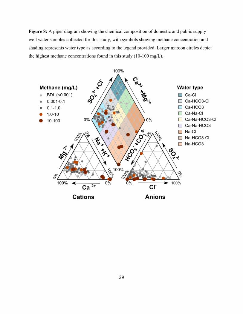
purpose of this broad study, although the Piper diagrams do show that mixing does occur. A Piper

11

diagram was used (Fig. 8) to illustrate which water type zone (i.e. Ca-rich or Na-rich) the samples

in this study cluster toward and the relation of each zone to methane concentrations.

3.5 Statistical Analysis of Data

MATLAB R2017b was used for statistical analysis of the data. The Mann-Whitney U

non-parametric test was used to analyze grouped data including: water type (Ca-rich vs. Na-

rich), topographic position (valley vs. upland), completion material (bedrock vs. sand and

gravel), and confinement (confined vs. unconfined). A non-parametric test was chosen due to the

skewed nature of the methane dataset as the majority of the samples fall near or below the

detection limit (BDL). Significance of continuous relationships among methane concentrations

and proximity parameters (e.g. distance to nearest gas well) were evaluated using Pearson,

Spearman, and Kendall τ coefficients. Pearson correlation coefficients describe the linear

correlation among continuous variables and are most suitable for datasets which are normally

distributed. The Spearman correlation coefficient is a non-parametric measure of dependence

between two variables using a ranking system and are not strongly influenced by outliers. The

Kendall τ coefficient measures the strength of association among two measured values also using

rank (Helsel and Hirsh, 2002; Christian, 2015).

4. Results

Methane concentrations range from below the detection limit (BDL) or <0.001 mg/L-84.6

mg/L with a median concentration of 0.0037 mg/L. Iodine concentrations range from 0-342 μg/L

with a median concentration of 4.31 μg/L. The groundwater well with the highest methane

12

concentration (OT1771) was drilled in a Devonian-aged confined bedrock aquifer in central NYS

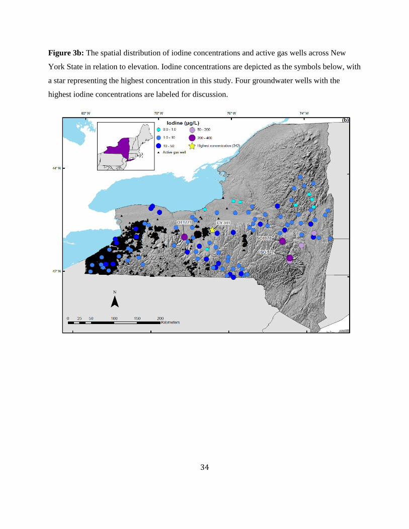
(Fig. 3a). The groundwater well with the highest iodine concentration (CY 311) was also found in

central NYS, roughly 61 km northeast of the well with the highest methane concentration and both

wells are approximately 10 and 12 km south of the Marcellus Shale outcrop (northern boundary)

in the Finger Lakes Region (Fig. 3b). The well with the highest iodine concentration in this study

was also completed in a confined Devonian bedrock aquifer. 6% of samples had dissolved methane

concentrations above 10 mg/L and 2% of which exceed the U.S. Office of Surface Mining and

Reclamation Enforcement hazard level of 28 mg/L (Eltschlager et al., 2001; Kappel and Nystrom,

2012; Fig. 4a). 54% of the dissolved methane samples fell between 0.001-10 mg/L while 40% lie

BDL. 95% of iodine concentrations fall below the average concentration for seawater which is

approximately 63 μg/L (Lu et al., 2014) where 5% of samples exceed the seawater average (Fig.

4b). In comparison to Project SWIFT (Christian et al., 2016), the range of methane and iodine has

doubled and tripled; respectively. This is likely due to this study covering a larger and more

geologically diverse study area with a lower sampling density.

Sedimentary bedrock tends to have wells with higher iodine and methane concentrations

in comparison to wells completed in or above crystalline bedrock. Iodine concentrations are found

highest when the sedimentary rock is organic-rich (e.g. Marcellus Shale). Where the bedrock is

crystalline in the study area, groundwater has low concentrations of bromine, iodine, and methane

(Fig. 5).

Two methods used in the literature to determine topographic position include the NHD

(National Hydrography Dataset) method and the Valley-Fill Aquifer method. These methods

classify topographic position differently (Fig. 6). The NHD method classifies 35 of the 108 total

13

wells as within a valley setting and 73 as within an upland setting (Fig. 6a). The Valley-Fill Aquifer

method considers 49 wells as being within a valley setting and 59 wells as being within an upland

setting (Fig. 6b). The Mann-Whitney U tests yield no significance differences among methane

concentrations in valleys as compared to uplands when classified using either the NHD method or

the Valley-Fill Aquifer method (p=0.98; p=0.29).

In this study, groundwater samples were classified and grouped based on water type. The

majority (82%) of samples are classified as Ca-rich (n=88), 16% of samples were classified as Na-

rich (n=17), and 2% as Mg-rich (n=2) (Fig. 7). Groundwater wells having a Na-rich water type

predominately had elevated methane concentrations >10 mg/L, whereas wells classified as having

a Ca-rich water type displayed a wide range of methane concentrations from BDL to >10 mg/L

(Fig. 8). The Mann-Whitney U test confirmed a significance between the distribution of methane

between Ca-rich and Na-rich water types (p=0.002); with median concentrations of 0.0028 and

0.27, respectively.

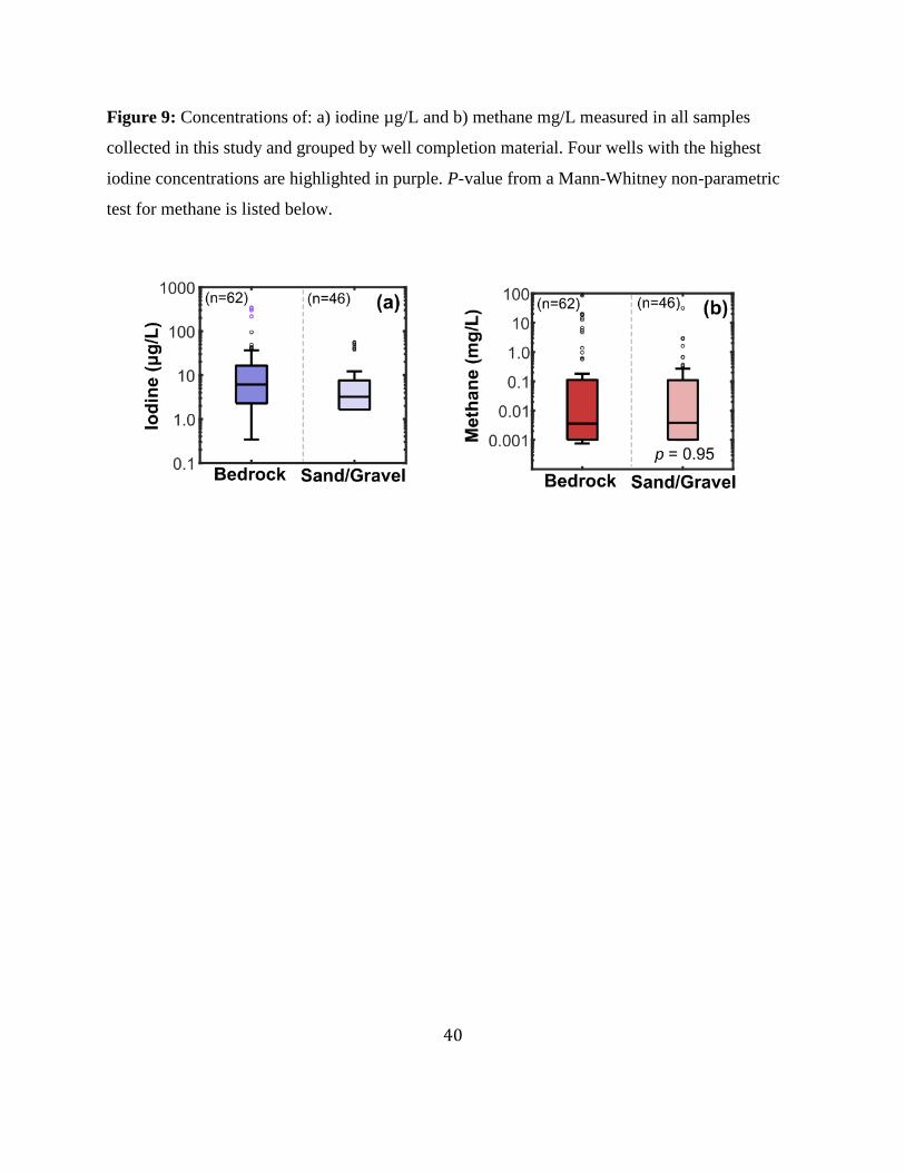
All groundwater samples collected in this study were separated into groups based on the well

completion material identified by the USGS. The two groups included wells completed in: 1)

bedrock and 2) sand and gravel (Fig. 9). The Mann-Whitney U test showed no significant

differences between methane concentrations of wells completed in bedrock compared to wells

completed in sand and gravel (p=0.96). Wells completed in bedrock had a larger range in

concentrations of dissolved methane in comparison to wells completed in sand and gravel. Wells

completed in bedrock had dissolved methane concentrations ranging between 0-85 mg/L; where

wells completed in sand and gravel had methane concentrations ranging between 0-31 mg/L. Five

wells fall within the monitoring action range of 10-28 mg/L and were completed in bedrock. Two

14

wells fall above the immediate action level of 28 mg/L, one completed in sand and gravel (31

mg/L) and the other completed in bedrock (85 mg/L). The four wells with the highest iodine

concentrations in this study were completed in bedrock (Table 4; Figure 3b).

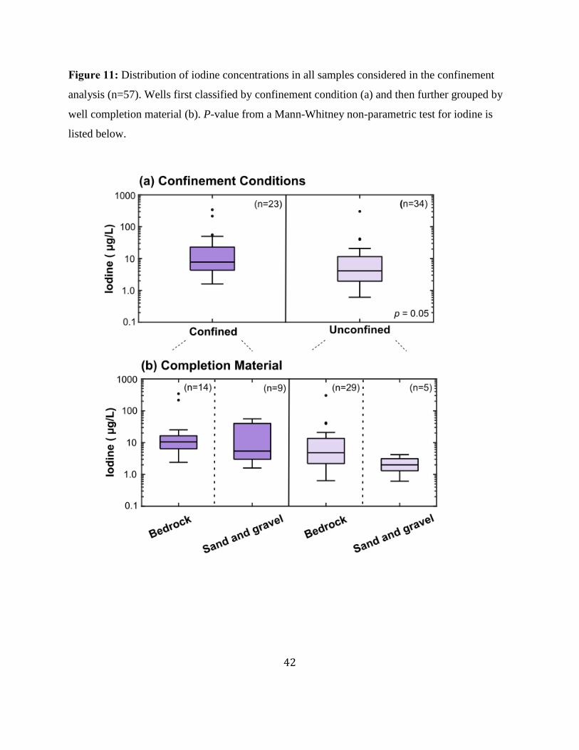
Fifty-seven groundwater wells met the suitable requirements (see Methods) and were

included in the confinement analysis. The wells that were considered to be drilled into confined

aquifers (n=23) typically had elevated concentrations of methane and iodine in comparison to wells

drilled into unconfined aquifers (n=34) (Fig. 10, Fig. 11) and overall a greater range in dissolved

methane (Fig. 10). The Mann-Whitney U test revealed that methane concentrations in confined

aquifer settings were significantly different (p=0.026) than methane concentrations of unconfined

aquifers with median methane concentrations of 0.01 and 0.001, respectively. This same test

showed that iodine concentrations are slightly significant (p=0.05) however not as significant as

the relationship among methane and confinement. Within this subset of samples, the conditions

resulting in the greatest occurrence of methane were determined to be that of wells completed in a

confined sand and gravel aquifer due to a higher median methane concentration in comparison to

confined bedrock wells. Conversely, wells finished in unconfined sand and gravel aquifers

generally had lower concentrations of methane (<0.01 mg/L). We provide a closer analysis of two

groundwater wells (CY 311 and SO1976) that exhibited the highest iodine concentrations

measured in this study (342 μg/L and 302 μg/L; respectively) to illustrate this concept (Fig. 3b).

The two wells are located in geographically different locations in NYS and are approximately 153

km apart (Fig. 15). Well CY 311 was determined to have been completed in a confined sand and

gravel aquifer, and well SO1976, in an unconfined sand and gravel aquifer (Table 4). Despite both

15

wells exhibiting an enrichment in total dissolved iodine, well CY 311 also had elevated methane

(18.5 mg/L), where well SO1976 did not (0.020 mg/L).

The potential for stray gas migration to both domestic and public supply groundwater wells

from historical gas production areas was assessed by groundwater well proximity to active

(n=6,814) and other gas wells (n=4,096) from available NYSDEC data

(http://www.dec.ny.gov/cfmx/extapps/GasOil/search/wells/index.cfm) (Fig.12). Other gas wells

refer to all remaining classifications including inactive, plugged, and abandoned, temporarily

abandoned, and unknown. This gas well dataset, displayed using a linear scale, shows a spike in

dissolved methane concentrations within close proximity to an existing active gas well and another

spike at approximately 100 km from an active gas well. When looking at the gas well data set on

a log scale there appears to be no correlation between distance to nearest active gas well and

measured methane concentrations in drinking water wells. However, when assessing the distance

to nearest non-active gas well, there appears to be higher methane concentrations within 50 km to

the nearest non-active gas well. The Pearson coefficient between methane concentrations and

proximity to active and other gas wells was not significant (p=0.41; p=0.45) however, the

Spearman and Kendall τ test suggest that there is a significant difference (Table 5).

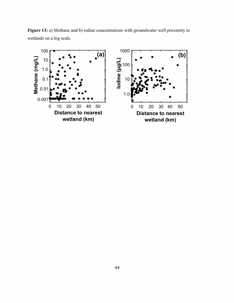
Wetland influence on groundwater concentrations of methane and iodine was assessed by

looking at well proximity to soils mapped and classified as a histosol. Histosols are one of the 12

orders of soil taxonomy, a soil order composed of organic material formed in bogs, peatlands, and

mucks. Seven wells in total are drilled through a histosol soil layer: three wells below latitude

43.25°N (CU1440, FU1629, and OW 503) and four wells above latitude 43.25°N (EX248, H 383,

H352, and WR1568) (Table 3). The seven wells had iodine concentrations ranging between 0.680

16

and 4.03 with an average of 1.66 μg/L. All wells drilled directly through a histosol soil layer had

methane concentrations that fall BDL, are low in iodine, and had a Ca-rich water type. The

relationship among methane and iodine concentrations with proximity to nearest wetland was

further assessed visually using a proximity plot and there was no apparent relationship (Fig. 13).

The Pearson test supported this and found no significance (p>0.05), while the Spearman and

Kendall τ coefficients between methane concentrations and wetland proximity hypothesized that

methane levels were significant and that concentrations decrease toward wetlands (Table 5).

Wells completed in Middle Devonian bedrock (Marcellus) and Upper Devonian bedrock

have both elevated iodine and bromine concentrations. Whereas wells finished in older bedrock

(Silurian and Ordovician aged) and crystalline bedrock units have lower concentrations of iodine

and bromine (Fig. 14a). In conjunction with low halogen concentrations, the older and crystalline

bedrock show low dissolved methane concentrations most commonly BDL. Middle Devonian and

Upper Devonian wells with elevated halogen concentrations display the highest methane

concentrations in this study (Fig. 14b). These Devonian bedrock wells with elevated methane

concentrations appear in the middle of NYS, between latitudes 42.2° and 43.0° N (Fig. 14c), and

primarily across western and central NYS, and the lower Mohawk RB.

5. Discussion

5.1 Controls on Groundwater Methane

As demonstrated in previous studies, the occurrence of methane in groundwater is

common in wells located above the Marcellus Shale. These studies have associated elevated

methane concentrations to: 1) a wells position within a topographic low (Molofsky et al., 2013;

17

Heisig and Scott, 2013; Christian et al., 2016; Wen et al., 2018); 2) Na-rich groundwater type

(McPhillips et al., 2014; Siegel et al., 2015; Christian et al., 2016); 3) proximity to existing gas

well (Osborn et al., 2011; Jackson et al., 2013); and 4) confinement conditions (Heisig and Scott,

2013). Additional controls evaluated in this study include: completion material and proximity to

wetlands.

5.1.1 Underlying Bedrock Geology

Iodine and methane concentrations rely strongly on bedrock type. Groundwater wells

drilled into sedimentary bedrock tend to have higher iodine and methane concentrations in

comparison to wells completed in or above crystalline bedrock. Concentrations are found highest

when the sedimentary rock is organic-rich (e.g. Marcellus Shale). This is due to methane and

iodine both deriving from organic-rich matter (Lu et al., 2014). Figure 5 shows that groundwater

wells drilled into crystalline bedrock in our study area contain groundwater that has low

concentrations of bromine, iodine, and methane.

5.1.2 Topographic Position

The hypothesis that elevated methane associated with topographic lows is derived from

the conceptual model that groundwater wells located in valleys are closer to the

freshwater/saltwater interface and deep groundwater charged with dissolved methane (Heisig and

Scott, 2013; Fig. 2). Past studies have had varying results when implementing topographic

position as a predictor for methane in groundwater. Molofsky et al., 2013 found that in a similar

study of Susquehanna County of northern Pennsylvania, methane concentrations were

18

significantly higher in wells located in a valley setting in comparison to wells in an upland

setting using a Mann-Whitney U test. Contrarily, other studies located in southern NYS found no

significance among methane concentration and topographic position (Jackson et al., 2013;

McPhillips et al., 2014).

In this study, the median concentrations for iodine are similar among uplands and valleys

among both methods (Fig. 6). Both methods show slightly higher median methane

concentrations in valley settings. For the purposes of this study, independent of the method used

(Valley-Fill Aquifer or NHD), topography does not act as a suitable indicator in locating

methane in groundwater (p>0.05).

5.1.3 Water Type

Past studies have revealed that higher methane concentrations are typically linked to deeper

groundwater classified as Na-rich (McPhillips et al., 2014; Siegel et al., 2015; Christian et al.,

2016). The association among methane and Na-rich water types is likely a result of carbonate

dissolution in the underlying shale and the cation exchange between calcium and sodium over long

residence times (Christian et al., 2016). The deep Na-rich water was saltwater that was present

during marine deposition during the development of the basin that had since been physically and

chemically altered (Siegel et al., 2015). These deep saline waters are likely charged with methane,

which is adumbrative of local bedrock or upwards seepage of methane from an underlying source

rock (Heisig and Scott, 2013). In this study, aside from a few outliers, Na-rich groundwater also

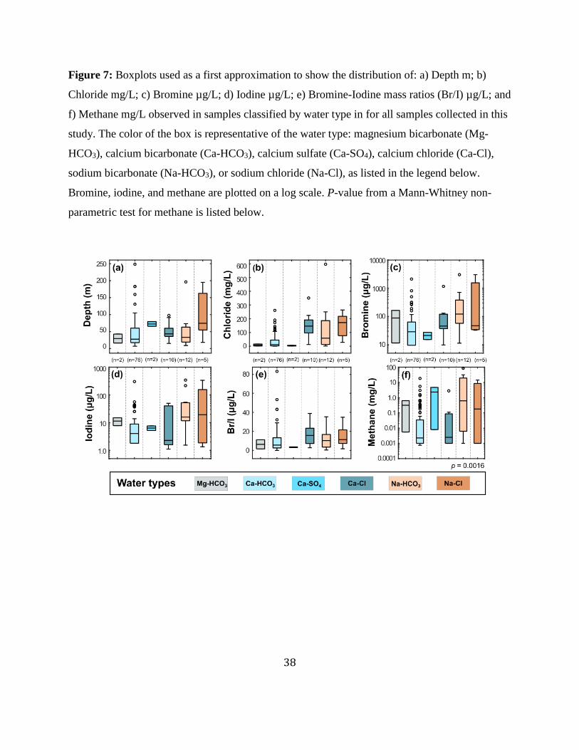
generally has greater methane compared to more Ca-rich waters (Fig. 8). Deeper groundwater in

particular tends to be Na-rich and have elevated chloride, bromine, iodine, and methane relative to

19

shallower Ca-rich groundwater (Fig. 7a). Chloride, bromine, and iodine are all found in higher

concentrations in the deeper Na-rich waters (Fig. 7b, 7c, 7d). Methane concentrations are also

elevated in deeper Na-rich water (Fig. 7f). Water type does not appear to play a large role in Br/I

mass ratios (Fig. 7e). However, Ca-HCO3 water type has the largest range in ratios likely due to

the larger sample size (n=76). The Piper diagram (Fig. 8) illustrates that most samples in this study

cluster in the Ca-rich (Ca-HCO3) zone and in this zone are samples with a broad range of methane

concentrations. Dissolved methane concentrations in the Ca-rich zone range from BDL to <100

mg/L. The Na-rich zone has a relatively consistent range of methane concentrations within

groundwater samples where concentrations of dissolved methane are generally found to be

between 10-100 mg/L. This work is in alignment with previous studies in that there is a significant

difference in methane concentrations among Ca-rich and Na-rich water types.

5.1.4 Confinement Conditions

Aquifer confinement has received little attention in literature with respect to water quality

in the Appalachian Basin. Heisig and Scott (2013) addressed confinement conditions and

suggested that the highest concentrations of methane occur in bedrock within valleys under

confined groundwater conditions. In this study, methane concentrations in confined aquifer

settings were significantly different than methane concentrations of unconfined aquifers. The

median methane concentration in confined aquifers completed in sand and gravel is greater than

that of bedrock however, there is no significant difference when further grouping confinement into

completion type (Fig. 10). Determining the degree of possible confinement proved difficult at

times where well logs were not available, which was almost half of the wells sampled.

20

Accordingly, for this part of our study, only half the entire data base was used which perhaps

biased these results because of the smaller data set.

Confinement conditions were also evaluated in regard to iodine concentrations. The highest

iodine concentration was in a confined bedrock well. Confined bedrock wells also had a greater

median iodine concentration relative to confined sand and gravel wells (Fig. 11). A slightly

significant difference in iodine concentrations amidst confined and unconfined aquifers was found

however there was no difference between iodine concentrations in bedrock and unconsolidated

material. Understanding the occurrence of iodine can aid in illustrating the behavior of methane in

connection to confinement conditions as there are instances where confinement does appear to be

a driver to higher methane concentrations. For example, two groundwater wells (CY 311 and

SO1978) located 153 km apart lie just above the methane-bearing Marcellus Shale (Fig. 3), well

SO1976 is shallow and is drilled into an unconfined aquifer that allows methane from the

Marcellus to escape to the atmosphere whereas, a thick confining layer of clayey-till penetrated by

well CY 311 acts as a trap and holds the dissolved methane in the subsurface and allow

concentrations of it to become higher (Fig. 15).

5.1.5 Proximity to Existing Gas Wells

Locations of active gas wells and the groundwater wells sampled in this study with

corresponding methane concentrations were plotted on a map to assess the spatial distribution (Fig.

3a). Natural gas well activity is prevalent in western NYS and decreases towards the east. Methane

concentrations >10mg/L appear across the state. However, in western NYS where gas activity is

dominant there are fewer wells with low methane in contrast to the other sampling regions.

21

Methane concentrations with groundwater well proximity to “active” and “other” gas wells was

addressed and on a linear scale and it visually appears that the groundwater wells in a closer

proximity to the gas wells contain higher methane (Fig. 12). Siegel et al., 2015 discussed that a

using a linear scale in this analysis is visually misleading and that when using a log-transformed

scale, concentration ranges do not visually appear significantly different for samples located at

closer distances to gas wells. Past studies have experienced various success when using proximity

to gas wells as a predictor of elevated methane. Some studies have attributed elevated methane

concentrations to proximity to gas wells (Osborn et al., 2011; Jackson et al., 2013), while other

recent studies found a lack of relationship among methane and distance gas wells (McPhillips et

al., 2014; Siegel et al., 2015; Christian et al., 2016).

In this study, elevated methane concentrations and proximity to existing gas wells do not

appear to be related and is further supported by the Pearson correlation test (p >0.05), however the

Spearman and Kendall τ statistical tests suggest that there is a significant difference (Table 5).

Although gas drilling could have influenced methane abundance, it is also plausible that these

water wells tap an aquifer elevated in dissolved methane due to its stratigraphic position above one

of the gas-yielding geologic strata in this region.

5.1.6 Proximity to Wetlands

Wetlands contribute between 15 to 45% of global methane emissions (Segers, 1997).

Methane production (methanogenesis) involves the microbial mineralization of organic carbon

under anaerobic conditions. This study found that all wells drilled through a histosol soil layer

which is indicative of a wetland environment were all found to have dissolved methane

22

concentrations falling BDL. The relationship among methane and iodine concentrations with

proximity to nearest wetland was further assessed and there was no visual relationship (Fig.13).

The Pearson statistical test correlation suggests that with regard to this study wetlands are not a

direct control on groundwater methane and iodine (p>0.05). The Spearman and Kendall τ

statistical tests suggest that methane concentrations decrease in closer proximity to wetlands

(Table 5). This could be due to the dominance of wetland regions in the northern part of the state

where the bedrock is crystalline and natural gas activity does not exist.

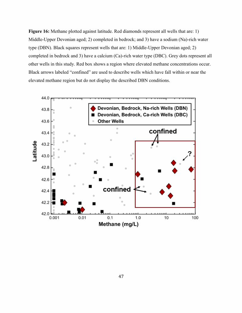
5.2. Methane Spatial Trends

Past studies agree that methane mostly occurs in groundwater in NYS when a

groundwater well is: 1) completed in bedrock; 2) Devonian in age; and 3) Na-rich. In NYS, wells

in higher latitudes (>43.2°) solely have lower methane concentrations and Ca- rich water types

whereas lower latitudes in NYS (<43.2°) have an array of methane concentrations and

corresponding water types. Figure 16 describes the ideal conditions for elevated methane

concentrations or a “sweet spot” in NYS. This location occurs between latitude 42.2° and 43.0 °

N. Fifteen wells fall within or near this “sweet spot” and seven of the 15 wells are completed in

Middle-Upper Devonian aged bedrock with a Na-rich water type displaying DBN (Devonian,

Bedrock, and Na-rich water type) conditions. These conditions are conducive for the presence of

elevated methane in groundwater wells. Eight wells within or near the sweet spot do not display

these conditions however five of the eight remaining wells can be described as having elevated

methane due to a confining layer which traps the methane below and does not allow it to escape.

23

5.3 Major Water Chemistry and Mixing Endmembers

A simple-two endmember mixing scenario between meteoric water and concentrations of

bromine and iodine measured in dilute road salt from the NYS Department of Transportation and

two known NYS Formations waters: Marcellus Formation (well D60) and Upper Devonian (well

D14) (Osborn et al., 2012) was created to examine the potential influence of road salt and deep

formation waters on shallow groundwater. D14 has the highest Br/I ratio from Osborn et al., 2013

and is drilled into an Upper Devonian organic-rich shale sampled in Chautauqua County of western

NYS. D60 has the lowest Br/I ratio and is drilled into Middle Devonian Marcellus Shale in Steuben

County in southern NYS. Very few deep wells in NYS have been studied for their bromine and

iodine concentrations (Lu et al., 2014). Groundwater from rock having a stronger organic signature

is enriched with iodine and therefore result in a lower Br/I ratio, whereas a stronger halite signature

leads to an increase in Br/I ratios (Lu et al., 2014).

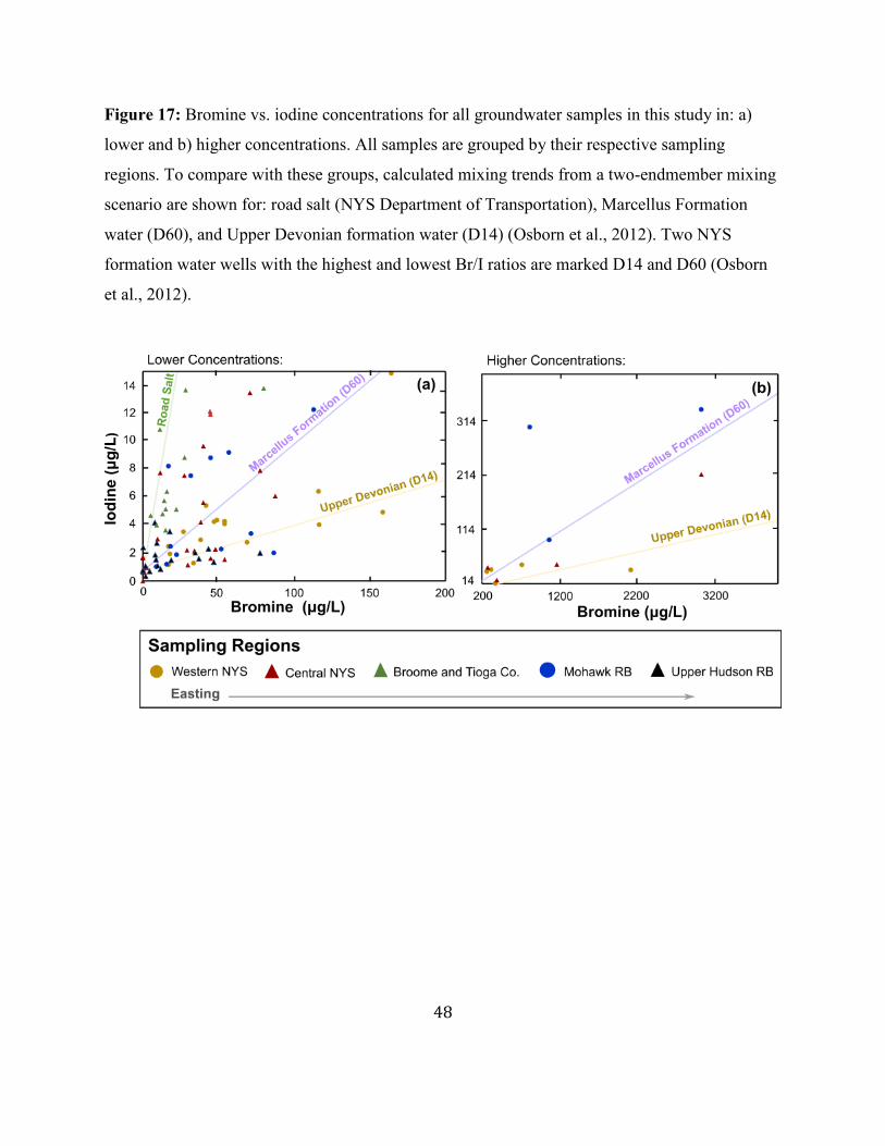
In this study, samples collected from western NYS generally fall along the D14 mixing

line with a Marcellus component. Broome and Tioga Co. samples fall along the road salt mixing

line (Fig. 17a). A few central NYS waters from wells plot directly on the Marcellus mixing line

(Fig. 17a) indicating an association among Marcellus formation waters and these wells. Upper

Hudson samples have low concentrations of both iodine and bromine due to being drilled

primarily in crystalline rock (Fig. 17a). Three out of the four wells with the highest iodine

concentrations in this study plot near the Marcellus mixing line (Fig.17b). This suggests that

these wells contain a portion of Marcellus Formation waters. This two-endmember mixing

scenario shows that road salt has an influence on the wells located in Broome and Tioga County

in southern NYS (Fig. 17a.) where wells sampled in western NYS tend to plot along the Upper

24

Devonian (D14) mixing line of western NYS suggesting that western NYS shallow groundwater

wells consist of diluted Upper Devonian formation waters from the rock deep below.

6. Summary and Conclusions

For this study, samples were collected from 108 groundwater wells from across NYS in

the late summer and fall of 2016 and 2017. Four distinct regions in NYS as outlined by the

USGS 305(b) Project: western NYS, the Mohawk River Basin, central NYS, the Upper Hudson

River Basin, and additional samples from Broome and Tioga County of south-central NYS were

examined. Over 200 constituents were included in the analysis including: methane and halogens

such as bromine, iodine, and chloride.

A number of natural and anthropogenic factors were assessed to determine the scenarios

most conducive for methane in groundwater. Factors evaluated included: underlying bedrock

geology, topographic position, water type, confinement conditions, proximity to existing gas

wells, and proximity to wetlands. In addition to the impacts of these controls on methane

occurrence, all wells included in this study, in addition to road salt and two known NYS

formation waters, were plotted on a two-endmember mixing scenario to examine the potential

influence of road salt and deep formation waters on potable groundwater. Samples collected

from western NYS generally fall along the D14 mixing line with a Marcellus component.

Broome and Tioga Co. samples fall along the road salt mixing line. A few central NYS waters

from wells plot directly on the Marcellus mixing line. Upper Hudson samples have low

concentrations of both iodine and bromine due to being drilled primarily in crystalline rock.

25

Three out of the four wells with the highest iodine concentrations in this study plot near the

Marcellus mixing line

Results of this study indicate that various controls can act as predictors for elevated

methane in groundwater. Incongruent with previous studies, a wells position within a valley did

not serve as a strong control. In contrast, general bedrock type, location of the well above the

methane-bearing Marcellus Shale, Na-rich water type, and a well displaying confined conditions

served as the strongest predictors for methane in shallow groundwater. In NYS, a groundwater

well completed in Devonian bedrock with Na-rich water type has the most likely scenario for

elevated methane conditions. Halogen concentrations, notably bromine and iodine, can

characterize saline formation waters naturally mixing with potable groundwaters. Groundwater

wells in this study sometimes contain water consisting of various amounts of Upper Devonian

and Marcellus formation waters from the rock deep below. This study shows that iodine in

conjunction with bromine can be utilized to identify the extent of formation water influence in

potable groundwater.

26

Tables

Table 1: Characterization of sampling regions across New York State (NYS) which are included

in this study.

Region and Year Drainage Basins Area (km2) General Geology

Western NYS

(2016) • Niagara River/Lake

Erie/Lake Ontario

• Allegheny River

13,831 Sedimentary

Mohawk River

Basin (2016) • Mohawk River 9,000 Sedimentary and

Crystalline

Central NYS

(2017) • Oswego-Seneca-

Oneida Rivers

• Lake Ontario

15,000 Sedimentary

Upper Hudson

River Basin (2017) • Upper Hudson River 6,440 Crystalline

Broome and Tioga

County (2017) • Susquehanna River 3,209 Sedimentary

27

Table 2: Geologic units for known bedrock wells in this study (n=60)

Geologic Age Unit of Completion Total Number of

Wells

Upper Devonian

Conneaut Group 2

Canadaway Group 6

Java-West Falls Formation 13

Sonyea Formation 6

Genesee Formation 1

Middle Devonian

Hamilton Formation 6

Onondaga Limestone 2

Lower Devonian Helderberg Group 1

Silurian

Lockport Dolomite 1

Clinton Group 3

Upper Ordovician

Queenston Shale 3

Oswego Sandstone 2

Middle Ordovician

Canajoharie Shale 2

Utica Shale 1

Middle and Lower

Ordovician

Beekmantown Group 1

Lower Cambrian

and Proterozoic

Nassau Formation 1

Unknown Crystalline Bedrock (Granite, Marble,

etc.)

9

Total 60

28

Table 3: Wells intersecting the histolsol layer in this study with associated New York State

(NYS) basin or river basin (RB) and water type. Dissolved methane and iodine concentrations

are also listed. BDL indicates “below the detection limit” which is 0.001 mg/L.

County Well

Number

Sampling Basin Water type Iodine (µg/L) Methane (mg/L)

CU1490 western NYS Ca-HCO3 4.03 BDL

OW 503 central NYS Ca-HCO3 1.72 BDL

FU1629 Mohawk RB Ca-HCO3 1.02 BDL

EX248 Upper Hudson RB Ca-Cl 2.3 BDL

H383 Upper Hudson RB Ca-HCO3 1.08 BDL

H352 Upper Hudson RB Ca-HCO3 0.68 BDL

WR1568 Upper Hudson RB Ca-HCO3 0.8 BDL

29

Table 4: Wells with the four highest iodine concentrations in this study are all finished in

bedrock and listed in the chart below.

County Well

Number

Iodine (µg/L) Methane (mg/L) Confinement

CY 311 342.20 18.50 Confined

SO 527 335.10 0.02 Unconfined

SO1976 302.70 0.03 Unconfined

OT1771 215.73 84.55 Confined

30

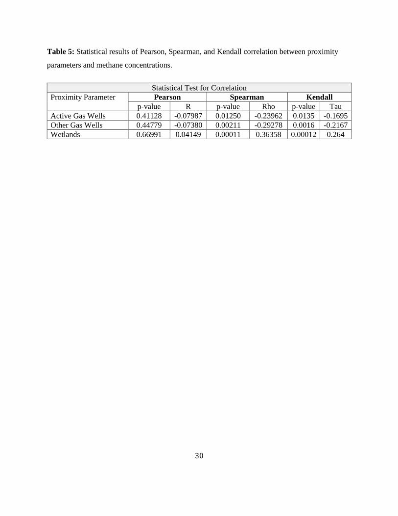
Table 5: Statistical results of Pearson, Spearman, and Kendall correlation between proximity

parameters and methane concentrations.

Statistical Test for Correlation

Proximity Parameter Pearson Spearman Kendall

p-value R p-value Rho p-value Tau

Active Gas Wells 0.41128 -0.07987 0.01250 -0.23962 0.0135 -0.1695

Other Gas Wells 0.44779 -0.07380 0.00211 -0.29278 0.0016 -0.2167

Wetlands 0.66991 0.04149 0.00011 0.36358 0.00012 0.264

31

Figures

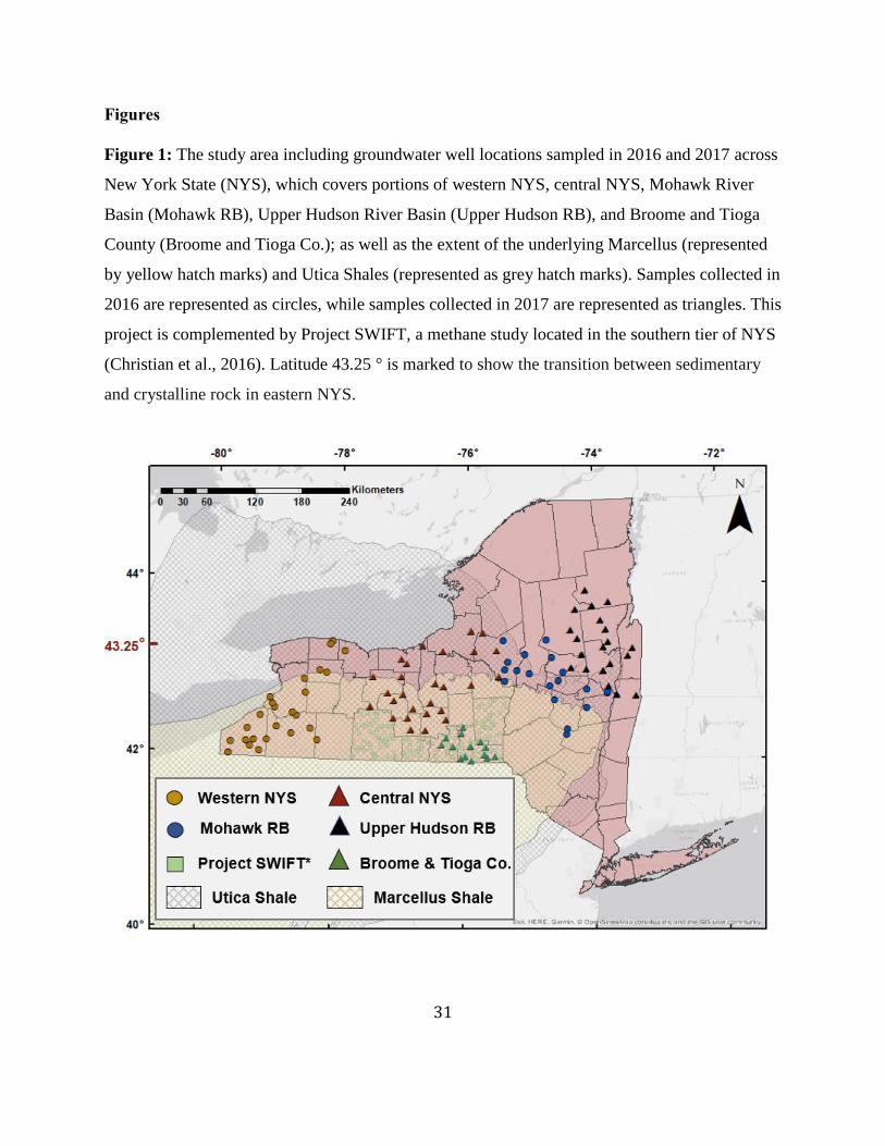
Figure 1: The study area including groundwater well locations sampled in 2016 and 2017 across

New York State (NYS), which covers portions of western NYS, central NYS, Mohawk River

Basin (Mohawk RB), Upper Hudson River Basin (Upper Hudson RB), and Broome and Tioga

County (Broome and Tioga Co.); as well as the extent of the underlying Marcellus (represented

by yellow hatch marks) and Utica Shales (represented as grey hatch marks). Samples collected in

2016 are represented as circles, while samples collected in 2017 are represented as triangles. This

project is complemented by Project SWIFT, a methane study located in the southern tier of NYS

(Christian et al., 2016). Latitude 43.25 ° is marked to show the transition between sedimentary

and crystalline rock in eastern NYS.

32

Figure 2: Conceptual diagram showing groundwater flow zones for both upland and valley

settings and the generalized water types. Dashed line represents the groundwater table. Other

symbols and water types are denoted in the key below.

33

Figure 3a: The spatial distribution of methane concentrations and active gas wells across New

York State in relation to elevation. Methane concentrations are depicted as the symbols below,

with a star representing the highest concentration in this study. Three groundwater wells are

labeled for discussion.

34

Figure 3b: The spatial distribution of iodine concentrations and active gas wells across New

York State in relation to elevation. Iodine concentrations are depicted as the symbols below, with

a star representing the highest concentration in this study. Four groundwater wells with the

highest iodine concentrations are labeled for discussion.

35

Figure 4: Histograms showing the relative frequency of iodine and methane occurrence in all

samples included in this study. Thresholds are represented by grey dashed lines: a) methane

actions levels (monitoring suggested when >10 mg/L and explosive hazard at >28 mg/L)

(Eltschlager et al., 2001; Kappel and Nystrom, 2012) and b) the average concentration of iodine

in seawater (>63µg/L) (Lu et al., 2014).

36

Figure 5: Map view of: a) iodine µg/L; b) bromine µg/L; and c) methane mg/L for all samples

collected in this study. Red box represents the rough separation between sedimentary rocks and

crystalline rocks at latitude 43.25 ° N and longitude 76° E.

37

Figure 6: Boxplots showing the distribution of dissolved methane mg/L and iodine µg/L

observed in all samples in this study classified by topographic position (upland vs valley).

Topographic position was delineated using: a) the NHD (national hydrography dataset) method

and b) the Valley-Fill Aquifer method. P-values from a Mann-Whitney non-parametric test for

methane are listed.

38

Figure 7: Boxplots used as a first approximation to show the distribution of: a) Depth m; b)

Chloride mg/L; c) Bromine µg/L; d) Iodine µg/L; e) Bromine-Iodine mass ratios (Br/I) µg/L; and

f) Methane mg/L observed in samples classified by water type in for all samples collected in this

study. The color of the box is representative of the water type: magnesium bicarbonate (Mg-

HCO3), calcium bicarbonate (Ca-HCO3), calcium sulfate (Ca-SO4), calcium chloride (Ca-Cl),

sodium bicarbonate (Na-HCO3), or sodium chloride (Na-Cl), as listed in the legend below.

Bromine, iodine, and methane are plotted on a log scale. P-value from a Mann-Whitney non-

parametric test for methane is listed below.

39

Figure 8: A piper diagram showing the chemical composition of domestic and public supply

well water samples collected for this study, with symbols showing methane concentration and

shading represents water type as according to the legend provided. Larger maroon circles depict

the highest methane concentrations found in this study (10-100 mg/L).

40

Figure 9: Concentrations of: a) iodine µg/L and b) methane mg/L measured in all samples

collected in this study and grouped by well completion material. Four wells with the highest

iodine concentrations are highlighted in purple. P-value from a Mann-Whitney non-parametric

test for methane is listed below.

41

Figure 10: Distribution of methane concentrations in all samples considered in the confinement

analysis (n=57). Wells are first classified by confinement condition (a) and then further grouped

by well completion material (b). P-value from a Mann-Whitney non-parametric test for methane

is listed below.

42

Figure 11: Distribution of iodine concentrations in all samples considered in the confinement

analysis (n=57). Wells first classified by confinement condition (a) and then further grouped by

well completion material (b). P-value from a Mann-Whitney non-parametric test for iodine is

listed below.

43

Figure 12: Methane concentrations with groundwater well proximity to “active” and “other” gas

wells on a linear (a and c) and log (b and d) scale.

44

Figure 13: a) Methane and b) iodine concentrations with groundwater well proximity to

wetlands on a log scale.

45

Figure 14: Mass ratios of iodine and bromine grouped by: a) bedrock; b) methane; and c)

latitude on log-transformed bivariate plots.

46

Figure 15: Conceptual diagram and table showing the local impacts of confinement on

corresponding iodine and methane (CH4) concentrations in groundwater. Red lines with arrows

represent CH4 escaping through fractures of the underlying methane-bearing bedrock.

47

Figure 16: Methane plotted against latitude. Red diamonds represent all wells that are: 1)

Middle-Upper Devonian aged; 2) completed in bedrock; and 3) have a sodium (Na)-rich water

type (DBN). Black squares represent wells that are: 1) Middle-Upper Devonian aged; 2)

completed in bedrock and 3) have a calcium (Ca)-rich water type (DBC). Grey dots represent all

other wells in this study. Red box shows a region where elevated methane concentrations occur.

Black arrows labeled “confined” are used to describe wells which have fall within or near the

elevated methane region but do not display the described DBN conditions.

48

Figure 17: Bromine vs. iodine concentrations for all groundwater samples in this study in: a)

lower and b) higher concentrations. All samples are grouped by their respective sampling

regions. To compare with these groups, calculated mixing trends from a two-endmember mixing

scenario are shown for: road salt (NYS Department of Transportation), Marcellus Formation

water (D60), and Upper Devonian formation water (D14) (Osborn et al., 2012). Two NYS

formation water wells with the highest and lowest Br/I ratios are marked D14 and D60 (Osborn

et al., 2012).

49

Appendix

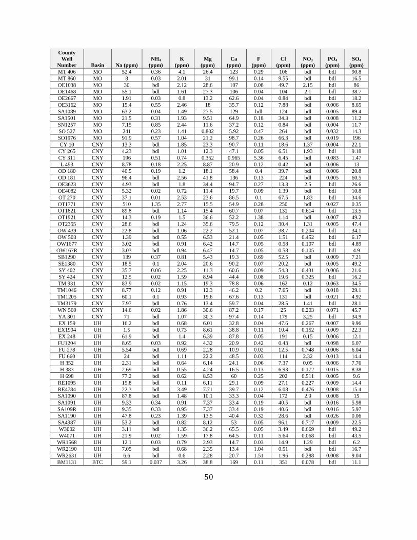
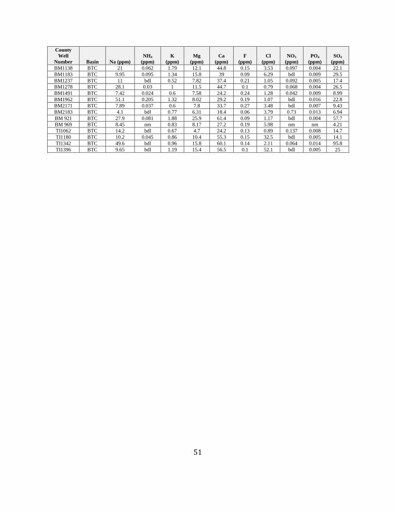
Table S1: Concentrations of major ions, dissolved methane, and halogens (n=108) for all

samples in this study (blank samples excluded). [bdl-below detection limit; nm-not measured;

County Designations - A-Albany; AG–Allegheny; BM-Broome; CT–Cattaraugus; CU–Chautauqua;

CY-Cayuga; E–Erie; EX-Essex; FU-Fulton; G-Greene; GS-Genesee; H-Hamilton; HE-Herkimer; L-

Lewis; MO-Monroe; MT-Montgomery; OD-Onondaga; OE-Oneida; OL-Orleans; OT-Otsego; OW-

Oswego; RE-Rensselaer; SA-Saratoga; SB-Steuben; SN-Schenectady; SO-Schoharie; SY-Schuyler; TI-

Tioga; TM-Tompkins; W-Washington; WE-West Chester; WN-Wayne; WR-Warren; YA-Yates: Basin

Designations - BTC-Broome and Tioga Counties; CNY- Central New York; MO-Mohawk Valley; WNY

–Western New York; UH-Upper Hudson: Constituent Designations – Ca-Calcium; Cl-Chloride; F-

Fluoride; K-Potassium; MG-Manganese; Na-Sodium; NH4-Ammonia; NO3-Nitrate; PO4-Phosphate;

SO4-Sulfate]

County

Well

Number Basin Na (ppm)

NH4

(ppm)

K

(ppm)

Mg

(ppm)

Ca

(ppm)

F

(ppm)

Cl

(ppm)

NO3

(ppm)

PO4

(ppm)

SO4

(ppm)

AG 265 WNY 38.1 0.11 1.68 7.08 33.2 0.08 65 1.71 0.188 10.4

CT 472 WNY 7.45 bdl 1.19 7.56 54.4 0.03 13.7 1.08 bdl 14.2

CT1176 WNY 4.54 0.01 1.25 6.98 41.4 0.17 2.19 0.368 bdl 19.5

CT2161 WNY 34 0.3 0.85 11.1 24.2 0.33 5.5 bdl 0.043 15.6

CT2884 WNY 5.17 0.01 0.56 4.75 29.5 0.07 5.15 0.196 0.006 11.3

CT2983 WNY 16.5 0.36 1.68 10.8 48.7 0.18 1.4 bdl bdl 13.8

CU 595 WNY 74.7 bdl 2.9 15.6 101 0.02 144 5.54 bdl 16.4

CU 809 WNY 65.2 bdl 1.71 8.91 69.9 0.04 133 1.5 bdl 15

CU1490 WNY 12.9 bdl 2.01 8.3 50.5 0.04 20.4 0.593 bdl 8.56

CU2131 WNY 37.9 bdl 2.59 14.9 88.9 0.05 65.8 1.09 bdl 12.4

CU2507 WNY 8.63 0.13 0.87 7.12 28.8 0.09 10.5 bdl 0.038 3.13

CU3272 WNY 4.73 0.11 0.69 11.8 51.3 0.11 15.1 bdl 0.029 18.3

CU3402 WNY 3.13 bdl 0.76 13.6 67.4 0.06 0.77 bdl 0.005 14.8

CU3542 WNY 27.2 0.49 3.05 17.7 77.7 0.25 120 bdl bdl 0.07

E1903 WNY 39.5 0.07 1.77 27.7 119 0.04 92.5 bdl 0.005 135

E1904 WNY 122 0.22 4.33 25.7 160 0.07 261 0.041 bdl 87.1

E2925 WNY 94.3 0.65 1.44 17.3 71.8 0.26 171 bdl bdl 2.36

E2925 WNY 25.9 0.37 1.19 14.2 56.2 0.26 35.2 bdl bdl 3.71

E3095 WNY 119 0.53 4.26 23.4 73 0.23 202 bdl 0.023 21

E3392 WNY 33.4 0.48 2.45 22.6 110 0.17 172 bdl bdl 8.14

GS 189 WNY 48.7 bdl 2.76 40.9 97.6 0.07 117 5.33 bdl 68.5

GS 216 WNY 103 0.02 3.61 31.6 114 0.1 190 0.455 bdl 41.3

MO1826 WNY 369 1.3 26.3 34.4 152 0.2 597 bdl bdl 106

OL 294 WNY 32.5 0.01 8.82 34.5 83.5 0.12 67.4 1.93 0.004 88.7

OL 356 WNY 53.2 0.35 7.22 43.5 61.5 0.27 15.5 bdl 0.005 49.2

A1169 MO 17.5 0.05 0.8 15.8 66.7 0.2 4.56 bdl 0.009 56.2

FU 606 MO 3.81 bdl 0.54 10.2 64.7 0.03 11.5 3.9 bdl 9.34

FU1629 MO 3.67 bdl 0.59 2 8.11 0.22 0.44 0.056 0.13 6.28

G 128 MO 96.7 0.12 0.51 2.31 12 0.25 92.5 bdl 0.068 0.46

H 244 MO 14.4 bdl 0.77 3.76 11.6 0.05 27.7 bdl 0.004 5.88

HE 622 MO 64.2 bdl 3.39 16.8 94.2 0.06 108 1.83 0.004 39.8

HE 624 MO 11.8 nm nm nm nm nm nm nm nm nm

HE2124 MO 94.9 1.34 8.15 5.06 10.9 0.91 19.4 0.562 0.008 30.9

50

County

Well

Number Basin Na (ppm)

NH4

(ppm)

K

(ppm)

Mg

(ppm)

Ca

(ppm)

F

(ppm)

Cl

(ppm)

NO3

(ppm)

PO4

(ppm)

SO4

(ppm)

MT 406 MO 52.4 0.36 4.1 26.4 123 0.29 106 bdl bdl 90.8

MT 860 MO 8 0.03 2.01 31 99.1 0.14 9.55 bdl bdl 16.5

OE1038 MO 30 bdl 2.12 28.6 107 0.08 49.7 2.15 bdl 86

OE1468 MO 55.1 bdl 1.61 27.3 106 0.04 104 2.1 bdl 38.7

OE2667 MO 1.91 0.03 0.8 13.2 62.6 0.04 0.84 bdl bdl 18.2

OE3162 MO 15.4 0.55 2.46 18 35.7 0.12 7.88 bdl 0.006 8.65

SA1089 MO 63.2 0.04 1.49 27.5 129 bdl 124 bdl 0.005 89.4

SA1501 MO 21.5 0.31 1.93 9.51 64.9 0.18 34.3 bdl 0.008 11.2

SN1257 MO 7.15 0.85 2.44 11.6 37.2 0.12 0.84 bdl 0.004 11.7

SO 527 MO 241 0.23 1.41 0.802 5.92 0.47 264 bdl 0.032 14.3

SO1976 MO 91.9 0.57 1.04 21.2 98.7 0.26 66.3 bdl 0.019 196

CY 10 CNY 13.3 bdl 1.85 23.3 90.7 0.11 18.6 1.37 0.004 22.1

CY 265 CNY 4.23 bdl 1.01 12.3 47.1 0.05 6.51 1.93 bdl 9.18

CY 311 CNY 196 0.51 0.74 0.352 0.965 5.36 6.45 bdl 0.083 1.47

L 493 CNY 8.78 0.18 2.25 8.87 20.9 0.12 0.42 bdl 0.006 13

OD 180 CNY 40.5 0.19 1.2 18.1 58.4 0.4 39.7 bdl 0.006 20.8

OD 181 CNY 96.4 bdl 2.56 41.8 136 0.13 224 bdl 0.005 60.5

OE3623 CNY 4.93 bdl 1.8 34.4 94.7 0.27 13.3 2.5 bdl 26.6

OE4082 CNY 5.32 0.02 0.72 11.4 19.7 0.09 1.39 bdl bdl 10.8

OT 270 CNY 37.1 0.01 2.53 23.6 86.5 0.1 67.5 1.83 bdl 34.6

OT1771 CNY 510 1.35 2.77 15.5 54.9 0.28 250 bdl 0.027 0.35

OT1821 CNY 89.8 bdl 1.14 15.4 60.7 0.07 131 0.614 bdl 13.5

OT1921 CNY 14.3 0.19 1.5 36.6 52.2 1.38 1.14 bdl 0.007 49.2

OT2355 CNY 28.6 bdl 1.24 35.6 79.5 0.12 30.4 1.31 0.005 47.4

OW 439 CNY 22.8 bdl 1.06 22.2 52.1 0.07 38.7 0.204 bdl 34.1

OW 503 CNY 1.39 bdl 0.55 6.53 21.4 0.05 1.51 0.452 bdl 6.17

OW1677 CNY 3.02 bdl 0.91 6.42 14.7 0.05 0.58 0.107 bdl 4.89

OW167R CNY 3.03 bdl 0.94 6.47 14.7 0.05 0.58 0.105 bdl 4.9

SB1290 CNY 139 0.37 0.81 5.43 19.3 0.69 52.5 bdl 0.009 7.21

SE1380 CNY 18.5 0.1 2.04 20.6 90.2 0.07 20.2 bdl 0.005 49.2

SY 402 CNY 35.7 0.06 2.25 11.3 60.6 0.09 54.3 0.431 0.006 21.6

SY 424 CNY 12.5 0.02 1.59 8.94 44.4 0.08 19.6 0.325 bdl 16.2

TM 931 CNY 83.9 0.02 1.15 19.3 78.8 0.06 162 0.12 0.063 34.5

TM1046 CNY 8.77 0.12 0.91 12.3 46.2 0.2 7.65 bdl 0.018 29.1

TM1205 CNY 60.1 0.1 0.93 19.6 67.6 0.13 131 bdl 0.021 4.92

TM3179 CNY 7.97 bdl 0.76 13.4 59.7 0.04 28.5 1.41 bdl 28.1

WN 560 CNY 14.6 0.02 1.86 30.6 87.2 0.17 25 0.203 0.071 45.7

YA 301 CNY 71 bdl 1.07 30.3 97.4 0.14 179 3.25 bdl 34.9

EX 159 UH 16.2 bdl 0.68 6.01 32.8 0.04 47.6 0.267 0.007 9.96

EX1994 UH 1.5 bdl 0.73 8.61 38.8 0.11 10.4 0.152 0.009 22.3

EX 248 UH 61.9 bdl 1.4 6.39 87.8 0.05 191 0.15 0.006 12.1

FU1204 UH 8.65 0.03 0.92 4.32 20.9 0.42 0.43 bdl 0.098 6.07

FU 278 UH 5.54 bdl 0.69 2.28 10.9 0.02 12.5 0.748 0.006 6.04

FU 660 UH 24 bdl 1.11 22.2 48.5 0.03 114 2.32 0.013 14.4

H 352 UH 2.31 bdl 0.64 6.14 24.1 0.06 7.37 0.05 0.006 7.76

H 383 UH 2.69 bdl 0.55 4.24 16.5 0.13 6.93 0.172 0.015 8.38

H 698 UH 77.2 bdl 0.62 8.53 60 0.25 202 0.511 0.005 9.6

RE1095 UH 15.8 bdl 0.11 6.11 29.1 0.09 27.1 0.227 0.009 14.4

RE4784 UH 22.3 bdl 3.49 7.71 39.7 0.12 6.08 0.476 0.008 15.4

SA1090 UH 87.8 bdl 1.48 10.1 33.3 0.04 172 2.9 0.008 15

SA1091 UH 9.33 0.34 0.91 7.37 33.4 0.19 40.5 bdl 0.016 5.98

SA109R UH 9.35 0.33 0.95 7.37 33.4 0.19 40.6 bdl 0.016 5.97

SA1190 UH 47.8 0.23 1.39 13.5 40.4 0.32 28.6 bdl 0.026 0.06

SA4987 UH 53.2 bdl 0.82 8.12 53 0.05 96.1 0.717 0.009 22.5

W3002 UH 3.11 bdl 1.35 36.2 65.5 0.05 3.49 0.669 bdl 49.2

W4071 UH 21.9 0.02 1.59 17.8 64.5 0.11 5.64 0.068 bdl 43.5

WR1568 UH 12.1 0.03 0.79 2.93 14.7 0.03 14.9 1.29 bdl 6.2

WR2190 UH 7.05 bdl 0.68 2.35 13.4 1.04 0.51 bdl bdl 16.7

WR2631 UH 6.6 bdl 0.6 2.28 20.7 1.51 1.96 0.288 0.008 9.04

BM1131 BTC 59.1 0.037 3.26 38.8 169 0.11 351 0.078 bdl 11.1

51

County

Well

Number Basin Na (ppm)

NH4

(ppm)

K

(ppm)

Mg

(ppm)

Ca

(ppm)

F

(ppm)

Cl

(ppm)

NO3

(ppm)

PO4

(ppm)

SO4

(ppm)

BM1138 BTC 21 0.062 1.79 12.1 44.8 0.15 3.53 0.097 0.004 22.1

BM1183 BTC 9.95 0.095 1.34 15.8 39 0.09 6.29 bdl 0.009 29.5

BM1237 BTC 11 bdl 0.52 7.82 37.4 0.21 1.05 0.092 0.005 17.4

BM1278 BTC 28.1 0.03 1 11.5 44.7 0.1 0.79 0.068 0.004 26.5

BM1491 BTC 7.42 0.024 0.6 7.58 24.2 0.24 1.28 0.042 0.009 8.99

BM1962 BTC 51.1 0.205 1.32 8.02 29.2 0.19 1.07 bdl 0.016 22.8

BM2171 BTC 7.89 0.037 0.6 7.8 33.7 0.27 3.48 bdl 0.007 9.43

BM2183 BTC 4.1 bdl 0.77 6.31 18.4 0.06 3.79 0.73 0.013 6.94

BM 921 BTC 27.9 0.081 1.88 25.9 61.4 0.09 1.17 bdl 0.004 57.7

BM 969 BTC 8.45 nm 0.83 8.17 27.2 0.19 5.98 nm nm 4.21

TI1062 BTC 14.2 bdl 0.67 4.7 24.2 0.13 0.89 0.137 0.008 14.7

TI1180 BTC 10.2 0.045 0.86 10.4 55.3 0.15 32.5 bdl 0.005 14.1

TI1342 BTC 49.6 bdl 0.96 15.8 60.1 0.14 2.11 0.064 0.014 95.8

TI1396 BTC 9.65 bdl 1.19 15.4 56.5 0.1 52.1 bdl 0.005 25

52

Table S2: Concentrations of dissolved methane and halogens for all samples in this study

(n=108). [bdl-below detection limit; Basin Designations - BTC-Broome and Tioga Counties;

CNY- Central New York; MO-Mohawk Valley; WNY –Western New York; UH-Upper Hudson]

County Well

Number Basin Methane (mg/L) Bromine (µg/L) Iodine (µg/L)

AG 265 WNY 0.2709 47.03 4.245

CT 472 WNY 0.2284 17.015 1.17

CT1176 WNY bdl 26.835 3.525

CT2161 WNY 0.0025 60.555 16.355

CT2884 WNY bdl 17.905 1.94

CT2983 WNY 0.0203 41.775 5.405

CU 595 WNY bdl 33.49 1.29

CU 809 WNY bdl 158.54 4.925

CU1490 WNY bdl 116.49 4.025

CU2131 WNY 0.3260 48.93 4.35

CU2507 WNY 0.0265 68.865 2.765

CU3272 WNY 1.5884 38.19 2.94

CU3402 WNY 0.0275 16.915 2.475

CU3542 WNY 18.254 263.16 36.565

E1903 WNY 0.0112 54.065 4.275

E1904 WNY 0.0293 317.71 40.145

E2925 WNY 20.431 373.40 14.6

E2925 WNY 5.5332 2109.5 39.51

E3095 WNY 0.9604 130.39 15.595

E3392 WNY 1.3661 189.72 41.63

GS 189 WNY 0.5623 54.04 4.085

GS 216 WNY 0.1021 116.09 6.415

MO1826 WNY 0.0021 713.62 48.935

OL 294 WNY 0.0007 498.01 11.54

OL 356 WNY 0.0056 164.07 14.88

A1169 MO 0.0262 24.25 55.675

FU 606 MO bdl 22.235 1.88

FU1629 MO bdl 8.85 1.02

G 128 MO 14.343 1062.6 94.655

H 244 MO 0.1791 32.33 19.185

HE 622 MO bdl 71.495 3.395

HE 624 MO bdl 18.295 2.47

HE2124 MO 0.0117 112.86 12.27

MT 406 MO 0.0352 63.3 25.3

MT 860 MO 0.0059 56.85 9.2

OE1038 MO bdl 86.485 2.01

OE1468 MO bdl 51.795 2.285

OE2667 MO 0.0036 15.75 1.195

OE3162 MO 2.9821 31.68 7.535

SA1501 MO 0.3680 63.59 37.63

53

County Well

Number Basin Methane (mg/L) Bromine (µg/L) Iodine (µg/L)

SN1257 MO 0.0038 16.92 8.23

SO 527 MO 6.6508 3014.7 335.1

SO1976 MO 0.0288 812.56 302.7

CY 10 CNY 0.0035 34.03 2.15

CY 265 CNY bdl bdl bdl

CY 311 CNY 18.500 94.57 342.2

L 493 CNY 0.1820 0.285 0.89

OD 180 CNY 0.0345 274.65 44.09

OD 181 CNY 0.1115 130.74 40.19

OE3623 CNY 0.0015 44.81 1.625

OE4082 CNY 0.1090 9.76 3.01

OT 270 CNY bdl 87.48 6.08

OT1771 CNY 84.550 3016.4 215.73

OT1821 CNY 0.0010 54.035 1.53

OT1921 CNY 0.6255 11.51 7.75

OT2355 CNY 0.0010 29.72 1.15

OW 439 CNY 0.0030 29.18 2.21

OW 503 CNY bdl bdl 1.72

OW1677 CNY bdl 0.95 0.635

OW1677R CNY bdl 2.615 0.955

SB1290 CNY 12.450 392 20.83

SE1380 CNY 0.0455 70.785 13.475

SY 402 CNY 0.2770 77.46 7.91

SY 424 CNY 0.0050 38.26 4.2

TM 931 CNY 0.0865 40.02 5.61

TM1046 CNY 0.0055 40 9.66

TM1205 CNY 2.8000 1161.6 49.71

TM3179 CNY bdl bdl 0.61

WN 560 CNY 0.0015 bdl 1.65

WN1109 CNY 4.7350 27.4 7.55

YA 301 CNY bdl 47.99 2.27

EX 159 UH 0.0040 18.755 1.49

EX1994 UH bdl 8.71 1.53

EX 248 UH bdl 43.38 2.3

FU1204 UH 0.0025 7.915 4.18

FU 278 UH bdl 9.715 1.095

FU 660 UH bdl 37.09 1.59

H 352 UH bdl 4.48 0.685

H 383 UH bdl 1.725 1.075

H 698 UH bdl 46.91 1.345

RE1095 UH bdl 9.255 2.71

RE4784 UH bdl 17.77 3.535

SA1090 UH bdl 34.62 2.02

SA1091 UH 0.6660 44.68 11.925

SA1091R UH 0.6615 44.345 12.135

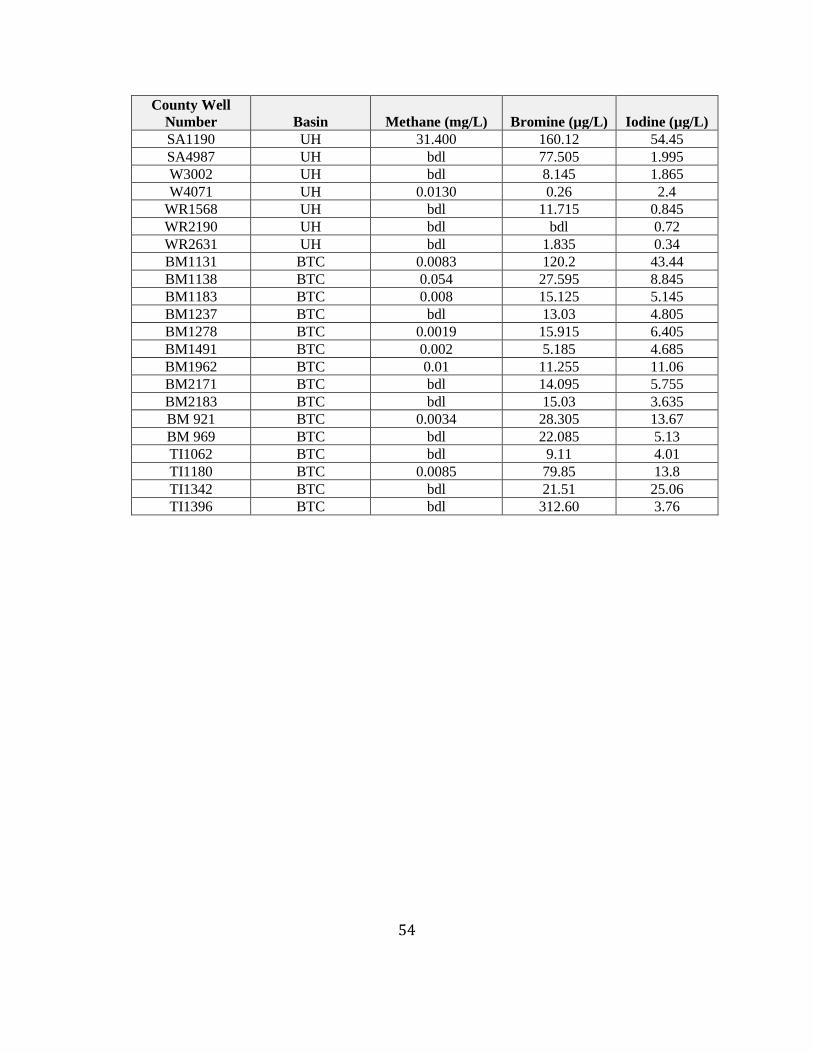
54

County Well

Number Basin Methane (mg/L) Bromine (µg/L) Iodine (µg/L)

SA1190 UH 31.400 160.12 54.45

SA4987 UH bdl 77.505 1.995

W3002 UH bdl 8.145 1.865

W4071 UH 0.0130 0.26 2.4

WR1568 UH bdl 11.715 0.845

WR2190 UH bdl bdl 0.72

WR2631 UH bdl 1.835 0.34

BM1131 BTC 0.0083 120.2 43.44

BM1138 BTC 0.054 27.595 8.845

BM1183 BTC 0.008 15.125 5.145

BM1237 BTC bdl 13.03 4.805

BM1278 BTC 0.0019 15.915 6.405

BM1491 BTC 0.002 5.185 4.685

BM1962 BTC 0.01 11.255 11.06

BM2171 BTC bdl 14.095 5.755

BM2183 BTC bdl 15.03 3.635

BM 921 BTC 0.0034 28.305 13.67

BM 969 BTC bdl 22.085 5.13

TI1062 BTC bdl 9.11 4.01

TI1180 BTC 0.0085 79.85 13.8

TI1342 BTC bdl 21.51 25.06

TI1396 BTC bdl 312.60 3.76

55

References

Alvarez, F., Reich, M., Snyder, G., Perez-Fodich, A., Muramatsu, Yasuyuki, M., Daniele, L., and

Fehn, U., 2016, Iodine budget in surface waters from Atacama: Natural and

iodine sources revealed by halogen geochemistry and iodine-129 isotopes: Applied

Geochemistry, v. 68, p. 53-63.

Christian, K., Methane Occurrence in Domestic Wells Overlying the Marcellus Shale. Thesis,

Syracuse University, Syracuse, NY, 2015.

Christian, K.M., Lautz, L.K., Hoke, G., Siegel, D.I., Lu, Z., and Kessler, J., 2016, Methane

occurrence is associated with sodium-rich valley waters in domestic wells overlying the

Marcellus shale in New York State: Water Resources Research, v. 52, p. 206-226.

Colton, G.W., 1970, The Appalachian Basin - its depositional sequences and their geologic

relationships, In: Fisher, G.W., Pettijohn, F.J., Reed, J.C.,Weaver, K.N., eds., Studies of

Appalachian Geology, Central and southern: Interscience Publishers, New York.

Davis, S.N., Whittemore, D.O., and Fabryka-Martin, J., 1998, Uses of Chloride/Bromide ratios

in studies of potable water: Ground Water, v.36, n.2, p. 338-350.

de Witt, W., Roen, J.B., and Wallace, L.G., 1993, Stratigraphy of Devonian black shales and

associated rocks in the Appalachian Basin, eds., Petroleum geology of the Devonian and

Mississippian black shale of eastern North America: U.S. Geological Survey Bulletin, p.

B1-B57.

Elderfield, H., Truesdale, V. W., 1980., On the biophilic nature of iodine in seawater: Earth and

Planetary Science Letters, v.50, p.105-114.

56

Eltschlager, K.K., Hawkins, J.W., Ehler, W.C., and Baldassare, Fred, 2001, Technical measures

for the investigation and mitigation of fugitive methane hazards in areas of coal mining:

U.S. Department of the Interior, Office of Surface Mining Reclamation and Enforcement,

p. 125.

Fehn, U., 2012, Tracing Crustal Fluids: Applications of Natural 129I and 36Cl: Annual Review of

Earth and Planetary Sciences, v. 40, p. 45-67.

Fisher, D. W., Isachsen, Y. W., and Rickard, L. V., 1970, Geologic map of New York State:

New York State Museum Map and Chart Series no. 15, Finger Lakes and Niagara sheets,

scale 1:250,000.

Gutchess, K. M., Jin, L. Lautz, L. K., Shaw, S. B., Zhou, X., and Lu, Z., 2016, Chloride sources

in urban and rural headwater catchments, central New York. Sciences of the Total

Environment, v. 565, p. 462-472.

Heisig, P.M., and Scott, T.M., 2013, Occurrence of Methane in Groundwater of South-Central

New York State, 2012-Systematic Evaluation of a Glaciated Region by Hydrogeologic

Setting: U.S. Geological Survey Scientific Investigations Report 2013-5190 ,p. 1-44.

Helsel, D.R., and Hirsch, R.M., 2002, Statistical methods in water resources: U.S. Geological

Survey Techniques of Water Resources Investigations, book 4, Cpt. A3.

Isachen, Y. W., Landing, E., Lauber, J.M., Rickard, L. V., and Rogers, W. B., 2000, Geology of

New York-A simplified account (second edition): Albany, N.Y., New York State

Museum/Geological Survey, p. 294.

Jackson, R. E., Vengosh, R. B., Darrah, T. H., Warner, N. R., Down, A., Poreda, R. J., Osborn,

S. G., Zhao, K. G., and Karr, J. D., 2013, Increased stray gas abundance in a subset of

57

drinking water wells near Marcellus shale gas extraction: PNAS, v. 110, n. 28, p. 11250-

11255.

Johnson, J. D., Graney, J. R., Capo, R. C., and Stewart, B. W., 2015, Identification and

quantification of regional brine and road salt sources in watersheds along the New

York/Pennsylvania border, USA: Applied Geochemistry, v. 60, p. 37-50.

Kappel, W. M., and Nystrom, E. A., 2012, Dissolved methane in New York groundwater, 1999-

2011, U.S. Geol. Survey. Open File Rep., 2012-1162, p.1-6.

Kerr, R. A., 2010, Natural gas from shale bursts onto the scene: Science, v.328, p.1624-1626.

Lautz, L. K., Hoke, G. D., Lu, Z., Siegel, D. I., Christian, K., Kessler, J., and Teale, N. G., 2014,

Using discriminant analysis to determine sources of salinity in shallow groundwater prior

to hydraulic fracturing: Environmental Science & Technology, v. 48, p. 16.

Li, J., Zhou, H., Wang, Y., Xie, X., and Qian, K., 2017, Sorption and speciation of iodine

in groundwater system: The roles of organic matter and organic-mineral complexes:

Journal of Contaminant Hydrology, v. 201, p. 39-47.

Lu, Z., Hummel, S. T., Lautz, L. K., Hoke, G. D., Zhou, Z., Leone, J., and Siegel, D. I., 2014,

Iodine as a sensitive tracer for detecting influence of organic-rich shale in shallow

groundwater: Applied Geochemistry, p. 1-8.

McPhillips, L. E., Creamer, A. E., Rahm B. G., and Walter, M. T., 2014, Assessing dissolved

methane patterns in central New York groundwater: Journal of Hydrology, p. 57-73.

Molofsky, L. J., Connor, J. A., Wylie, A.S., Wagner, T., and Farhat, S. K.,2013, Evaluation of

Methane Sources in Groundwater in Northeastern Pennsylvania: Groundwater, v. 51,

n.3, p. 333-349.

Moran, J.E., Fehn, U., and Hanor, J.S., 1995, Determination of source ages and migration

58

patterns of brines from the U.S. Gulf Coast basin using 129I: Geochimica et

Cosmochimica Acta, v. 59, n. 24, p. 5055-5069.

New York State Department of Environmental Conservation (NYSDEC), 2012. Oil and Gas

SearchableDatabase.http://www.dec.ny.gov/cfmx/extapps/GasOil/search/wells/index.cfm

(accessed July 2017).

New York State Department of Environmental Conservation (NYSDEC), 2008. Unconsolidated

Aquifers at 1:250,000. http://gis.ny.gov/gisdata/metadata/nysdec.uncon_aqui.html

(accessed July 2017)

Osborn, S.G., McIntosh, J.C., Hanor, J.S., and Biddulph, D., 2012. Iodine-129, 87Sr/86Sr, and

trace elemental geochemistry of northern Appalachian Basin brines: Evidence for

basinal-scale fluid migration and clay mineral diagenesis: American Journal of Science,

v. 312, p. 263-287.

Osborn, S. G., Vengosh, A., Warner, N. R., and Jackson R. B., 2011, Methane contamination

of drinking water accompanying gas-well drilling and hydraulic fracturing: PNAS, v.

108, n. 20, p. 8172-8176.

Panno, S.V., Hackley, K.C., Hwang, H.H., Greenberg, S.E., Krapac, I.G., Landsberger, and S.,

O’Kelly, D.J., 2006, Characterization and Identification of Na-Cl Sources in Ground-

water: Ground Water, v. 44, no. 2, p 176-187.

Reddy, J. E., 2014, Groundwater quality in central New York, 2012: U.S. Geological Survey

Open-File Report 2014-1226, p. 13.

Roen, J.B., 1984, Geology of the Devonian black shales of the Appalachian Basin:

Organic Geochemistry, v.5, p. 241-254.

59

Ryder, R. T., Burruss, R. C., and Hatch, J. R., 1998, Black Shale source rocks in the Cambrian

and Ordovician of the central Appalachian basin, USA: American Association of

Petroleum Geologists Bulletin, v. 82, no. 3, p. 412-441.

Scott, T. M., and Nystrom, E. A., 2014, Groundwater quality in the Upper Hudson River Basin,

New York, 2012: U.S. Geological Survey Open-File Report 2014-1084, p. 21.

Segers, R., 1998, Methane Production and methane consumption: a review of processes

underlying wetland methane fluxes: Biogeochemistry, v. 41, p. 23-51.

Siegel, D. I., Smith, B., Perry, E., Bothun, R., and Hollingsworth, M., 2015, Pre-drilling water

quality data of groundwater prior to shale gas drilling in the Appalachian Basin: Analysis

of the Chesapeake Energy Corporation dataset: Applied Geochemistry, v. 63, p 37-57.

Siegel, D. I., Azzolina, N. A., Smith, B. J., Perry, A. E., and Bothun, R. L., 2015, Methane

Concentrations in Water Wells Unrelated to Proximity to Existing Oil and Gas Wells in

Northeastern Pennsylvania: Environmental Science and Technology, v. 49, p.4106-4112.

Soeder, D.J., 2010, The marcellus shale: Resources and reservations: Eos, v.91, p.277-288.

United States Department of Agriculture (USDA) Natural Resources Conservation Service,2014.

Digital General Soil Map of the United States (STATSGO2)

http://websoilsurvey.nrcs.usda.gov/ (accessed February 2018)

United States Environmental Protection Agency, 1997, Guidelines for preparation of the

comprehensive state water quality assessments 305(b) reports and electronic updates:

U.S. Environmental Protection Agency, EPA 841-B-97-002A and EPA.

United States Geologic Survey, National Hydrography Dataset (NHD), 2011,

http://www.nhd.usgs.gov/ (accessed July 2017).

60

Wen, T., Niu, X., Gonzales, M., Zheng, G., Li, Z., and Brantley, S., 2018, Big Groundwater Data

Sets Reveal Possible Rare Contamination Amid Otherwise Improved Water Quality for

Some Analytes in a Region of Marcellus Shale Development: Environmental Science and

Technology, v. 52, p. 7149-7159.

Williams, J.H., 2010, Evaluation of well logs for determining the presence of freshwater,

saltwater, and gas above the Marcellus Shale in Chemung, Tioga, and Broome

Counties, New York: U.S. Geological Survey Scientific Investigations Report 2010–

5224, 27 p., http://pubs.usgs. gov/sir/2010/5224/.

61

Vita

Shannon Garvin

Email: Shannon.garvin11@gmail.com

EDUCATION

M.S., Earth Sciences at Syracuse University, Syracuse, NY (August 2018)

B.S., Geology at State University of New York at Cortland, Cortland, NY (December 2015)

A.A.S., Liberal Arts at Onondaga Community College, Syracuse, NY (December 2012)

EXPERIENCE

Teaching Assistant at Syracuse University, Syracuse, NY (2016-2018)

Hydrologic Technician at U.S. Geological Survey (USGS), Ithaca, NY (2014-2017)

Substitute Teacher at Sandy Creek Central School, Sandy Creek, NY (2016)

Instructional Support Technician at SUNY Cortland Geology Department, Cortland, NY (2015)

PRESENTATIONS

Garvin, Shannon R., Gutchess, Kristina M., 2018. Evaluating the natural controls of dissolved

CH4 and halogens in groundwater. Waggoner Geology Graduate Seminar, Syracuse, New York.

Oral Presentation.

Garvin, Shannon R., Gutchess, Kristina M., Lu, Wanyi, Kappel, William M., Lautz, Laura K.,

Lu, Zunli. 2017. Groundwater iodine across New York State: Potential linkage to methane?

Geological Society of America Abstracts with Programs, 49(6). doi: 10.1130/abs/2017AM-

306257. Poster Presentation.

Garvin, Shannon R., Gutchess, Kristina M., 2017. Using iodine as a natural tracer in

groundwater across New York State. Waggoner Geology Graduate Seminar, Syracuse, New

York. Oral Presentation.

Garvin, Shannon R., Gutchess, Kristina M., Lu, Wanyi., Lu, Zunli. 2017. Iodine as a natural

tracer in groundwater across New York State. Central New York Earth Science Student

Symposium, Syracuse, New York. Poster Presentation.

SKILLS

MATLAB; ArcGIS; Geochemist’s Workbench; Microsoft Word; Excel; PowerPoint; Adobe

Illustrator; Inkscape; R; Pix4D

ACTIVITIES

Geology Graduate Organization Student Affairs Coordinator (2017-2018)