Assessing credit quality from the equity market: can a structural approach forecast credit ratings?

Can J Adm SciCopyright © 2007 ASAC. Published by John Wiley & Sons, Ltd. 212 24(3), 212–228

Assessing Credit Quality from the Equity Market: Can a Structural Approach Forecast Credit Ratings?Yu DuRBC Financial Group

Wulin Suo*Queen’s University

Canadian Journal of Administrative SciencesRevue canadienne des sciences de l’administration24: 212–228 (2007)Published online 29 August 2007 in Wiley Interscience (www.interscience.wiley.com). DOI: 10.1002/CJAS.27

We are grateful for the comments and suggestions from the Editor, Jason Wei, and the two anonymous referees, as well as Edward Altman, Darrel Duffi e, Kim Huynh, Louis Gagnon, Lew Johnson, Frank Milne and Lynnette Purda. Financial support from SSHRC and Queen’s School of Business are gratefully acknowledged.*Please address correspondence to: Wulin Suo, School of Business, Queen’s University, 99 University Avenue, Kingston, Ontario, Canada K7L 3N6. Email: [email protected]

AbstractWe investigate the empirical performance of default probability prediction based on Merton’s (1974) struc-tural credit risk model. More specifi cally, we study if distance-to-default is a suffi cient statistic for the equity market information concerning the credit quality of the debt-issuing fi rm. We show that a simple reduced form model outperforms the Merton (1974) model for both in-sample fi tting and out-of-sample predictability for credit ratings, and that both can be greatly improved by including the fi rm’s equity value as an additional vari-able. Moreover, the empirical performance of this hybrid model is very similar to that of the simple reduced form model. As a result, we conclude that distant-to-default alone does not adequately capture the fi rm’s credit quality information from the equity market. Copyright © 2007 ASAC. Published by John Wiley & Sons, Ltd.

JEL Classifi cation: G13, G33

Keywords: Credit rating, default probability, distance-to-default, structural credit risk model

RésuméDans cet article, nous évaluons la performance empirique de la prédiction de probabilité de non-remboursement à partir du modèle de risque de crédit structurel de Merton (1974). Plus particulièrement, nous cherchons à exami-ner dans quelle mesure la “distance par rapport à la défaillance” (distance-to-default) est une statistique suf-fi sante pour l’information du marché d’actions concer-nant la qualité du crédit de la compagnie émettrice. Nous démontrons qu’un modèle simple de formule réduite donne de meilleurs résultats à la fois pour l’agencement échantillonné et pour la prédictibilité hors-échantillon que le modèle de Merton (1974), et que ces deux résultats peuvent être encore plus précis si la valeur comptable de la fi rme est prise en compte comme variable supplé-mentaire. Par ailleurs, la performance empirique de ce modèle hybride est très semblable à celle du modèle simple de forme réduite. Aussi concluons-nous que la distance par rapport à la défaillance ne rend pas fi dèle-ment compte de l’information concernant la qualité du crédit provenant du marché d’actions. Copyright © 2007 ASAC. Published by John Wiley & Sons, Ltd.

Mots-clés : Cote de crédit; probabilité de défaut; distance par rapport à la défaillance; modèle de risque de crédit structurel

ASSESSING CREDIT QUALITY FROM THE EQUITY MARKET DU & SUO


The proper assessment of credit risk has always been important to fi nancial institutions. Recently, fi nancial institutions have devoted even more resources to the development of tools that will adequately assess and manage the credit risk in their portfolios because, under the new Basel accord (Basel II) issued by the Basel Com-mittee on Banking Supervision, regulatory capital will be determined using a bank’s internal assessments of the probabilities that its counterparts will default. One popular approach to assessing credit risk involves the Merton (1974) model, where debts issued by a company are treated as derivatives written on the fi rm’s underlying assets. This approach allows one to establish structural relationships among the fi rm’s debt, equity, and the asset value. Using equity market data, one can generate a quantity that determines the default probability of a debt-issuing fi rm. These types of models, usually referred to as structural models, can thus establish relationships between default probabilities and some credit risk measures that are analytic functions of various relevant factors. Such models have become increasingly popular in recent years. In this paper, we investigate whether the credit risk measures inferred from structural credit risk models are adequate to refl ect the credit risk information contained in those individual factors or, more generally, whether structural models can provide a better alternative to assessing fi rms’ credit quality than those traditional statistical methods.

Empirical studies on the performance of structural models generally focus on the relationship between default risk and corporate bonds yields (see Eom, Helwege, & Huang, 2004 and the references therein). Few empirical studies have been conducted on the rela-tionship between the actual default frequency and the theoretical default probability calculated from these models. Notable exceptions include Hillegeist, Keating, Cram, and Lundstedt (2004) and Vassalou and Xing (2004). Hillegeist et al. fi nd that structural default prob-ability measures contain relatively more information than Altman’s Z-Score and Ohlson’s O-Score. Using measures calculated from structural credit risk models as proxies to fi rms’ default risks, Vassalou and Xing fi nd that the Fama-French SMB and HML factors (see Fama & French, 1996) do not proxy the default factors. More-over, in practice, Moody’s KMV has been using the Merton (1974) type of structural models to predict the default probabilities of individual fi rms.

On the other hand, fi rms’ credit qualities have tradi-tionally been linked to their credit ratings, which are ordinal measures assigned by rating agencies to refl ect the debt-issuing fi rms’ ability to serve their debts. The rating process includes quantitative as well as qualitative and legal analysis. While similar approaches are used by

different rating agencies when assigning credit ratings, and although some agencies are more forthcoming than others in describing the procedures they follow in assign-ing or reviewing a rating, they all use proprietary methods to do so. For these reasons, various models have been proposed to predict a fi rm’s credit rating changes based on publicly available information. Research in this area includes Blume, Lim, and MacKinlay (1998), Horrigan (1966), Kaplan, and Urwitz (1979), Pogue and Soldofsky (1969), and West (1973) among others. Despite the skep-ticism from rating agencies, these models have been fairly successful in explaining and predicting the ratings of a large cross-section of corporate bonds.

Most of the studies concerning credit rating forecast-ing have focused on either determining the factors affect-ing a fi rm’s credit rating or building better econometric techniques. Popular approaches include hazard rate models, logistic type of models, and discriminant analy-sis, where usually the chosen independent variables enter the estimation process in a linear way. Little attention has been paid to the possible structural interactions among the independent variables and to the possible non-linear effect of the covariates.

Although credit ratings are not designed to pinpoint the precise probability of default, one should expect a close relationship between these two measures if one believes that credit ratings are sound measures of the credit qualities of the debt-issuing fi rms. Default proba-bilities derived from structural credit risk models, at least prima facie, provide a promising alternative for predict-ing credit rating changes. It is thus important to investi-gate whether these models can indeed perform better than the traditional statistical models in terms of in-sample fi tting and out-of-sample prediction of credit rating changes. More specifi cally, we are interested in answering the following question: do the credit risk mea-sures calculated from the structural models have better explanatory and predictive power for a fi rm’s credit quality, which we assume are represented by the fi rm’s credit rating, than the linear combination of those vari-ables appearing in the structural models?

In spite of the importance of this subject, few studies have been conducted, with the exceptions of Geske and Delianedis (1998); KMV (1998); Leland (2002); and Vassalou and Xing (2003). Geske and Delianedis docu-ment that the default probability calculated from struc-tural models contains enough information that both the rating migration and defaults are detected months before the actual credit events. Vassalou and Xing employ the default measure calculated from structural models and study the equity returns following changes in credit ratings. KMV compares the credit risk measure obtained from the credit transition matrix provided by rating



agencies with KMV’s Expected Default Frequency (EDF) and fi nds that risk measurement systems based upon the rating transition matrix are subject to large errors. It reports that fi rms’ expected default frequency with different ratings often overlaps. Leland (2002) com-pares the Leland and Toft (1996) model, which is based on an endogenously determined default boundary, with the Longstaff and Schwartz (1995) model, where default boundary is exogenously specifi ed. He fi nds that the Leland and Toft model can generate a default probability term structure that fi ts better with the actual default prob-ability term structure for a specifi c class of fi rms within the same credit rating.

None of these studies, however, address the issue of whether the default measures calculated from structural models are adequate in refl ecting the credit information contained in the variables used as inputs to the models, such as the fi rm’s equity value and its volatility and the debt-to-equity ratio, among others. Moreover, it is also worthwhile to investigate whether the default measures calculated from the structural models can actually predict a fi rm’s credit risk, which we assume is refl ected by the fi rm’s credit rating, better than the ad hoc reduced form models. Alternatively, we investigated whether the default risk measures calculated from structural models adequately refl ect all the information in the individual factors concerning the fi rm’s credit quality. We attempted to answer these questions. We also compared the perfor-mance of these two types of approaches based on the performance of both their in-sample fi ttings and out-of-sample predictions.

Another motivation for our study originates from the well-documented empirical fi ndings that structural credit risk models have diffi culties in generating the large credit spreads observed in the corporate bond market, espe-cially when the maturity of the bond is relatively short. Huang and Huang (2003) argue that credit risk contrib-utes to only a fraction of credit spread (see also Ericsson & Renault, 2006). Instead, they attribute a major part of credit spread to the liquidity of corporate bonds. Their results are based on the assumption that the structural credit risk models used in their study are adequate to capture and price credit risk. As pointed out by Huang and Huang, their method creates a joint hypothesis problem: when a calculated credit yield spread based on a model fails to match the empirically observed yield spread, one may also conclude that the model is mis-specifi ed. In this paper, we shed some light on whether structural credit risk models can indeed adequately capture the default risks in the fi rst place.

Our empirical results suggest that Merton’s theoreti-cal default measure, which is represented by distance-to-default, is not a suffi cient statistic of the market

information concerning the credit quality of the issuing fi rm. Both in-sample fi t and out-of-sample prediction can be greatly improved by using a hybrid model that includes the equity value of the fi rm as an additional independent variable, which suggests that the market information regarding the fi rm’s credit quality is not fully captured through the single quantity of distance-to-default. More-over, we fi nd that the performance of this hybrid model differs little from a simple statistical model, where the main inputs for the structural model are used as explana-tory variables. For this reason, we conclude that the credit risk measures calculated from the structural models are inadequate to capture the credit risk information con-tained in the variables for the model, and thus structural models do not necessarily provide any additional ability in capturing credit risks. A recent work by Bharath and Shumway (2004) reaches similar conclusions when his-torical default data are used in their analysis. On the other hand, a recent paper by Benos and Papanastasopoulos (2005) fi nds that by combining the risk-neutral distance-to-default measure and accounting factors one can predict credit rating changes fairly well.

The remainder of this paper is organized as follows: The next section introduces the structural credit risk models. Following this, we summarize how to compute the default probability measures for individual fi rms by using their equity prices. We then describe the economet-ric methodology used in this paper. Following this description, we present the data used and report the summary statistics. Before concluding we provide the empirical tests, discuss the estimation results, and inves-tigate forecasting abilities of both structural and statisti-cal models. The Appendix presents the estimation method for the hazard rate model.

Structural Credit Risk Model

In the seminal work of Merton (1974), the fi rm’s asset value VA is assumed to follow a lognormal process in the following form:

dV

Vdt dzAt

At

A A t= +µ σ , (1)

where mA and sA are assumed to be constants that describe the instantaneous growth rate and volatility of the fi rm’s asset value, respectively; and zt is a standard Brownian motion. If we also assume that there is only one class of debt that pays no coupon and has a maturity time T and principal amount X, then the fi rm is in default if the fi rm’s asset value is less than X at time T.

The equity of the fi rm, VE, can be regarded as a call option written on the fi rm’s underlying asset and can be



expressed through the Black and Scholes option pricing formula:

V V N d Xe N dE ArT= ( ) − ( )−

1 2 , (2)

where

dV X r T

Td d T

A A

A

A1

2

2 1

2=

( ) + +( )= −

ln, ,

σσ

σ (3)

r is the risk-free interest rate and N(·) is the cumulative probability function for standard normal distribution. The current value of the debt is given by VA – VE.

Models based on this approach are usually referred to as structural models. They include the following basic elements:

• Risk-free interest rate process: This specifi es the dynamics of the interest rate without default risk. It is assumed to be constant in the Merton model (1974).

• Asset value process: The expected rate of return (including risk premium) and volatility of the asset value process refl ect the expected business growth opportunities and the business risk, respectively.

• Face value of debt: The level of debt determines the leverage ratio of the fi rm, which is an important indicator of the issuing fi rm’s credit quality.

• Default boundary: This specifi es the asset level that causes the fi rm to default when its asset value declines to this level. In the Merton model, this boundary is characterized by the face value of the debt.

• Recovery rate: This postulates the value that the debt holders receive per $1 of the value of the debt when the fi rm is indeed in default. This rate is not needed in the Merton model.

These components of structural credit risk models in-clude all the variables considered important by rating agencies when assigning credit ratings. Structural models differ from traditional statistical ones in that the former specify how each component interacts with one another.

Various extensions of the Merton (1974) model have been proposed, including Collin-Dufresne and Goldstein (2001); Duffi e and Lando (2001); Hull and White (1995), Leland (1998); Leland and Toft (1996); and Longstaff and Schwartz (1995), among others. Although the mathematical derivations of these models appear to be complex, the basic idea is simple; once we specify the stochastic process of a random variable, then theoreti-cally we are able to calculate, either analytically or numerically, the probabilities of that variable being higher or lower than a prespecifi ed boundary at any later point of time. For example, in the Merton model, the fi rm’s asset value is assumed to follow a lognormal process, with the face value of the fi rm’s debt being the default boundary. The probability that the fi rm’s asset

value falls below the default boundary can be easily cal-culated analytically. In general, a structural credit risk model with a closed form solution for the corporate bond price has an analytical expression for the risk-neutral default probability, which is the theoretical measure of credit quality with structural explanation for the interac-tion of different risk factors and their effects on default. KMV Corporation adopted this approach when assessing default probabilities based on the Merton model. In closing this section, it is important to note that when deriving the physical default probability, what matters is the physical expected asset return rather than the risk-free interest rates used in the option pricing formula for the pricing purpose.

Estimation of Default Probability from Equity Data

If we assume that the fi rm’s asset value follows the process given in (1), its debt amount of X matures at time T and the fi rm is in default if its asset value falls below level X at time T, then its default probability is given by:

P P V Xdef A T= ≤( ), ,

where P is the physical or empirical probability. The fi rm’s asset value at time T can be written as:

ln ln ,,V V T zA T A A A A T( ) = ( ) + −( ) +µ σ σ2 2

where VA is the current value of the fi rm’s asset. The fi rm’s default probability can be calculated as:

P P V X

NV X T

T

def A T

A A A

A

= ( ) ≤ ( )( )

= −( ) + −( )

ln ln

ln

,

µ σσ

2 2.

This result shows that the distance-to-default, defi ned as:

Dis ceV X T

TA A A

A

tan =( ) + −( )ln

,µ σ

σ

2 2 (4)

determines the fi rm’s default probability.1

Default happens when the ratio of the value of assets to debt is less than one. The distance-to-default measure indicates how many standard deviations the logarithm of this ratio needs to deviate from its mean before the fi rm defaults. In order to calculate this measure, we need to estimate the parameters mA and sA, which represent the fi rm’s asset growth rate and volatility, respectively. However, since the asset value is not traded, these param-eters cannot be directly observed from the market.

To compute the distance-to-default measure from equity values, we followed a similar procedure adopted



by KMV and Vassalou and Xing (2004).2 We consider the default probability for a one-year period. All of the fi rm’s debts were assumed due in one year, and the total amount of debt was approximated as the sum of all the short-term debts plus 50% of the long-term debts. The logic of this approach is that debts due within one year are more likely to cause default.

In order to calculate the asset value’s growth rate mA and volatility sA, we fi rst estimated the volatility of its equity sE as the standard deviation of its equity returns during the past twelve months. This estimation of sE is used as an initial value for the estimation of sA. Using this initial estimation of sA, we can obtain a time series of asset values VA by inverting the equation (2) with market equity values and debt. The next step was to cal-culate the standard deviation of those values of VA. This standard deviation will be used as the value of sA for the next round of iteration. This process is repeated until the standard deviations of VA from two consecutive iterations converge.3 Once the monthly values of VA are obtained, we can compute the growth rate mA as the mean return. Interest rates used in the calculation are the one-year constant maturity T-bill rates observed at the end of each month.

Alternatively, asset volatility and asset value can be calculated with the following equation:

σ σEA

E

A

V

V= ∆ , (5)

where ∆ is the hedge ratio N(d1) from equation (2). There are two unknown variables, VA and sA, and two equa-tions, (2) and (5), that are straightforward to solve.4 The drawback, however, is that equation (5) only holds instantaneously.

As pointed out by KMV (2002) and Vassalou and Xing (2004), the usual assumption that a fi rm’s asset value follows a lognormal distribution may not be appro-priate. For default measurement, the likelihood of large adverse changes in the relationship of the asset value to the fi rm’s default point is critical to the accurate deter-mination of the default probability. These changes may result from changes in asset value or changes in the fi rm’s leverage. In fact, KMV fi rst measures the distance-to-default as the number of standard deviations the asset value is from default. Then the distance-to-default values are mapped to historical default data to determine the corresponding default probability (see KMV for details).5

Econometric Methodology

Most of the corporate bankruptcy literature uses static, cross-sectional specifi cation for default estima-

tion. However, Shumway (2001) shows that hazard rate models are more suitable for forecasting bankruptcy than the single-period models used previously in the litera-ture. To overcome the diffi culty in estimating hazard rate models with time-varying covariates, Shumway demon-strates that hazard rate models can be estimated from the simple logistic type of models plus panel data, called the dynamic logistic model. In order to estimate the hazard rate model in the case of credit ratings, which include the default state as a special case, Du (2003) extends Shum-way’s binomial single-cycle model to a multinomial and multicycle hazard rate model and shows that this model is also equivalent to a logistic type of model plus panel data. The proof of the equivalence is presented in the Appendix. We applied hazard rate models, or the dynamic logistic model, to conduct the statistical analysis.

Variables involved in computing the measure of distance-to-default included the following: risk-free interest rate r, fi rm’s equity value VA,6 its volatility sE, fi rm’s book value of debt X, and the growth rate of the fi rm’s asset value mA. Thus, a naive statistical credit rating model employing equity market information takes the following form:

Z I ercept V

V

XDummy

t E t E t

E tt t

= + +

+ + +

nt β β σ

β ε

1 2

3

, ,

, , (6)

where Zt is the latent credit quality score that jointly determines the probabilities of credit ratings and Dummyt is the vector representing the year dummies variables. In addition, Intercept is a collection of cut-off points to separate the domain of the latent continuous variables Zt into several intervals with each interval corresponding to a specifi c credit rating. Year dummies are included in the independent variables set to capture some time-varying effects, such as the changes in credit rating policies docu-mented by Blume et al. (1998). When one takes the dis-tance-to-default measure Distance as the only independent variable as suggested by the structural credit risk model in the third section, the competing logistic model is constructed as follows:

Z Intercept Dis ce Dummyt t t t= + + +β εtan , (7)

where the distance-to-default measure Distancet is defi ned by equation (4).

Data and Summary Statistics

Each fi rm’s current debt and long-term debt were obtained from the annual COMPUSTAT database. Fol-lowing the approach adopted by KMV (2002) and Vas-salou and Xing (2004), we used the “Debt in One Year”



plus half the “Long Term Debt” as the book value of a fi rm’s total debt. Monthly equity value data were also collected from COMPUSTAT. Although the amount of the long-term debt to be included is arbitrary because coupon payments of a fi rm are unobservable, this choice was sensible and adequately captures the fi nancing con-straints of a fi rm (see KMV). Furthermore, many fi rms do not use a calendar fi scal year. In order to match ac-counting data with credit ratings and provide a meaning-ful explanation for the year dummies, we chose calendar year data.

Credit ratings of each fi rm, or issuer ratings, rather than the ratings for particular debts are collected from the 2002 annual COMPUSTAT, which contains monthly data for corporate ratings from 1985 to 2002. Instead of using the fi ner credit ratings provided by Standard and Poor (S&P), we follow the conventions of the literature to classify all the ratings into the following eight catego-ries: AAA, AA, A, BBB, BB, B, CCC, and CC. One advantage of employing issuer ratings instead of indi-vidual issue ratings is that the corporate rating will refl ect the fi nancial health and business risk of the fi rm rather than the bond-specifi c features. This also alleviates the concerns that loss given default also enters the decision process of bond rating agencies and helps to put more focus on the default probability of the fi rm represented by credit rating. Furthermore, cross-default clauses in debt contracts usually ensure that the default probabili-ties for each of the classes of debt for a fi rm are essen-tially the same; the default probability of the fi rm

determines the default probability for all the fi rm’s debt or counterpart obligations. Another advantage of using issuer credit ratings is that it greatly simplifi es the com-putation of structural default risk measures. More specifi -cally, option pricing models with multiple classes of debt are very complex and diffi cult to parameterize.

We collected monthly credit rating data for all fi rms with issuer credit ratings by S&P at the end of 1988. We used 1988 to compromise between two confl icting re-quirements: on one hand, more and more fi rms are rated by S&P over time, and in order to include more cross-sectional fi rms, it is desirable to begin with a later year.7 On the other hand, a longer time-series data set for each fi rm is preferred. In total, there were 1,508 fi rms in our sample. The individual fi rms in our sample were then tracked from 1989 to 2001.8 Following Vassalou and Xing (2004), monthly one-year constant maturity trea-sury bill rates were used for the one-year risk-free inter-est rates, and they were obtained from the Federal Reserve Board.

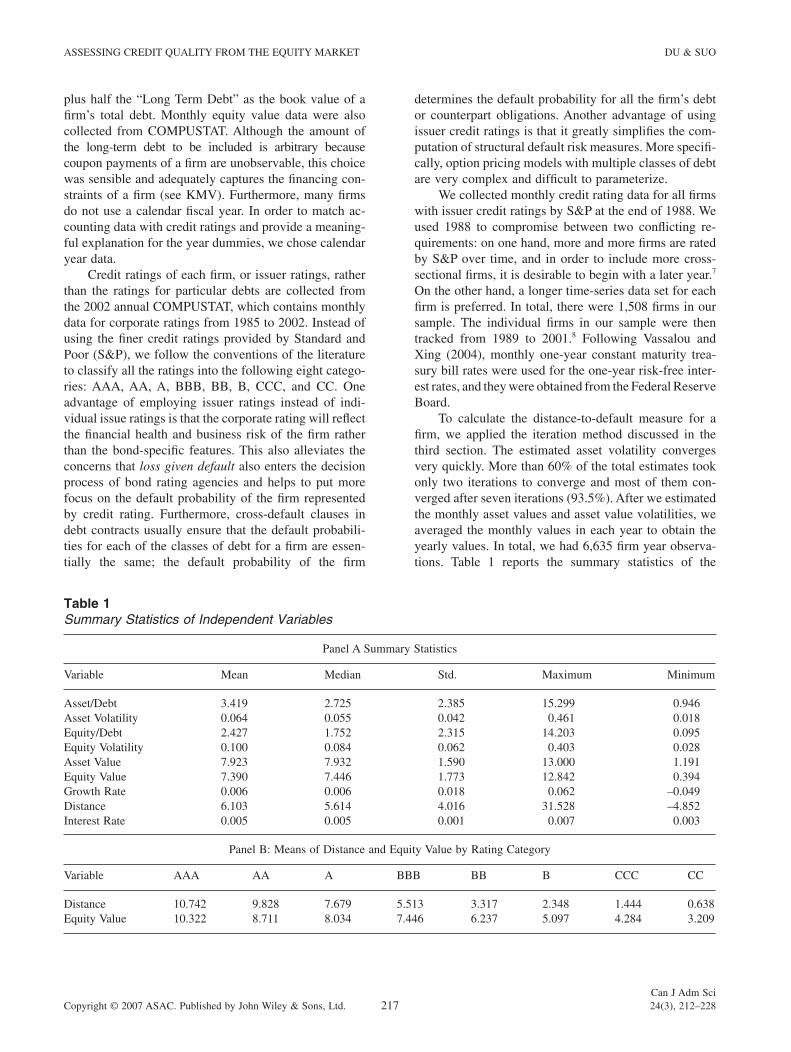
To calculate the distance-to-default measure for a fi rm, we applied the iteration method discussed in the third section. The estimated asset volatility converges very quickly. More than 60% of the total estimates took only two iterations to converge and most of them con-verged after seven iterations (93.5%). After we estimated the monthly asset values and asset value volatilities, we averaged the monthly values in each year to obtain the yearly values. In total, we had 6,635 fi rm year observa-tions. Table 1 reports the summary statistics of the

Table 1Summary Statistics of Independent Variables

Panel A Summary Statistics

Variable Mean Median Std. Maximum Minimum

Asset/Debt 3.419 2.725 2.385 15.299 0.946Asset Volatility 0.064 0.055 0.042 0.461 0.018Equity/Debt 2.427 1.752 2.315 14.203 0.095Equity Volatility 0.100 0.084 0.062 0.403 0.028Asset Value 7.923 7.932 1.590 13.000 1.191Equity Value 7.390 7.446 1.773 12.842 0.394Growth Rate 0.006 0.006 0.018 0.062 –0.049Distance 6.103 5.614 4.016 31.528 –4.852Interest Rate 0.005 0.005 0.001 0.007 0.003

Panel B: Means of Distance and Equity Value by Rating Category

Variable AAA AA A BBB BB B CCC CC

Distance 10.742 9.828 7.679 5.513 3.317 2.348 1.444 0.638Equity Value 10.322 8.711 8.034 7.446 6.237 5.097 4.284 3.209



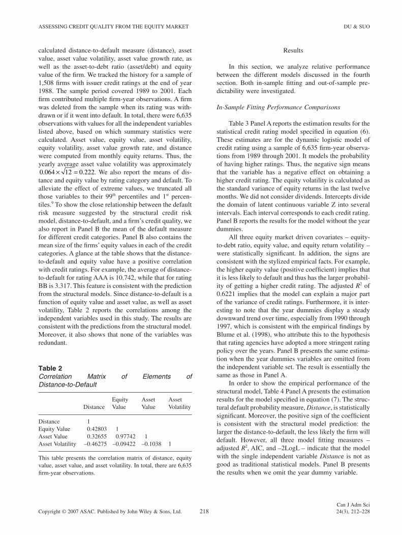
calculated distance-to-default measure (distance), asset value, asset value volatility, asset value growth rate, as well as the asset-to-debt ratio (asset/debt) and equity value of the fi rm. We tracked the history for a sample of 1,508 fi rms with issuer credit ratings at the end of year 1988. The sample period covered 1989 to 2001. Each fi rm contributed multiple fi rm-year observations. A fi rm was deleted from the sample when its rating was with-drawn or if it went into default. In total, there were 6,635 observations with values for all the independent variables listed above, based on which summary statistics were calculated. Asset value, equity value, asset volatility, equity volatility, asset value growth rate, and distance were computed from monthly equity returns. Thus, the yearly average asset value volatility was approximately 0 064 12 0 222. .× = . We also report the means of dis-tance and equity value by rating category and default. To alleviate the effect of extreme values, we truncated all those variables to their 99th percentiles and 1st percen-tiles.9 To show the close relationship between the default risk measure suggested by the structural credit risk model, distance-to-default, and a fi rm’s credit quality, we also report in Panel B the mean of the default measure for different credit categories. Panel B also contains the mean size of the fi rms’ equity values in each of the credit categories. A glance at the table shows that the distance-to-default and equity value have a positive correlation with credit ratings. For example, the average of distance-to-default for rating AAA is 10.742, while that for rating BB is 3.317. This feature is consistent with the prediction from the structural models. Since distance-to-default is a function of equity value and asset value, as well as asset volatility, Table 2 reports the correlations among the independent variables used in this study. The results are consistent with the predictions from the structural model. Moreover, it also shows that none of the variables was redundant.

Results

In this section, we analyze relative performance between the different models discussed in the fourth section. Both in-sample fi tting and out-of-sample pre-dictability were investigated.

In-Sample Fitting Performance Comparisons

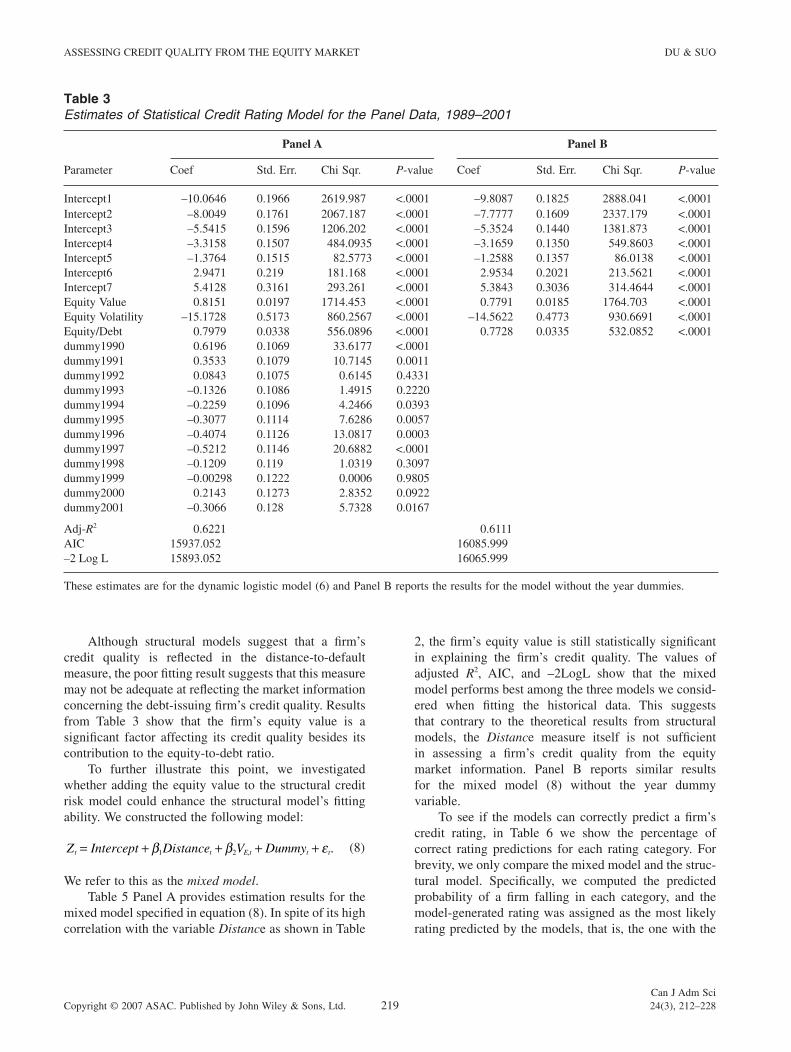
Table 3 Panel A reports the estimation results for the statistical credit rating model specifi ed in equation (6). These estimates are for the dynamic logistic model of credit rating using a sample of 6,635 fi rm-year observa-tions from 1989 through 2001. It models the probability of having higher ratings. Thus, the negative sign means that the variable has a negative effect on obtaining a higher credit rating. The equity volatility is calculated as the standard variance of equity returns in the last twelve months. We did not consider dividends. Intercepts divide the domain of latent continuous variable Z into several intervals. Each interval corresponds to each credit rating. Panel B reports the results for the model without the year dummies.

All three equity market driven covariates – equity-to-debt ratio, equity value, and equity return volatility – were statistically signifi cant. In addition, the signs are consistent with the stylized empirical facts. For example, the higher equity value (positive coeffi cient) implies that it is less likely to default and thus has the larger probabil-ity of getting a higher credit rating. The adjusted R2 of 0.6221 implies that the model can explain a major part of the variance of credit ratings. Furthermore, it is inter-esting to note that the year dummies display a steady downward trend over time, especially from 1990 through 1997, which is consistent with the empirical fi ndings by Blume et al. (1998), who attribute this to the hypothesis that rating agencies have adopted a more stringent rating policy over the years. Panel B presents the same estima-tion when the year dummies variables are omitted from the independent variable set. The result is essentially the same as those in Panel A.

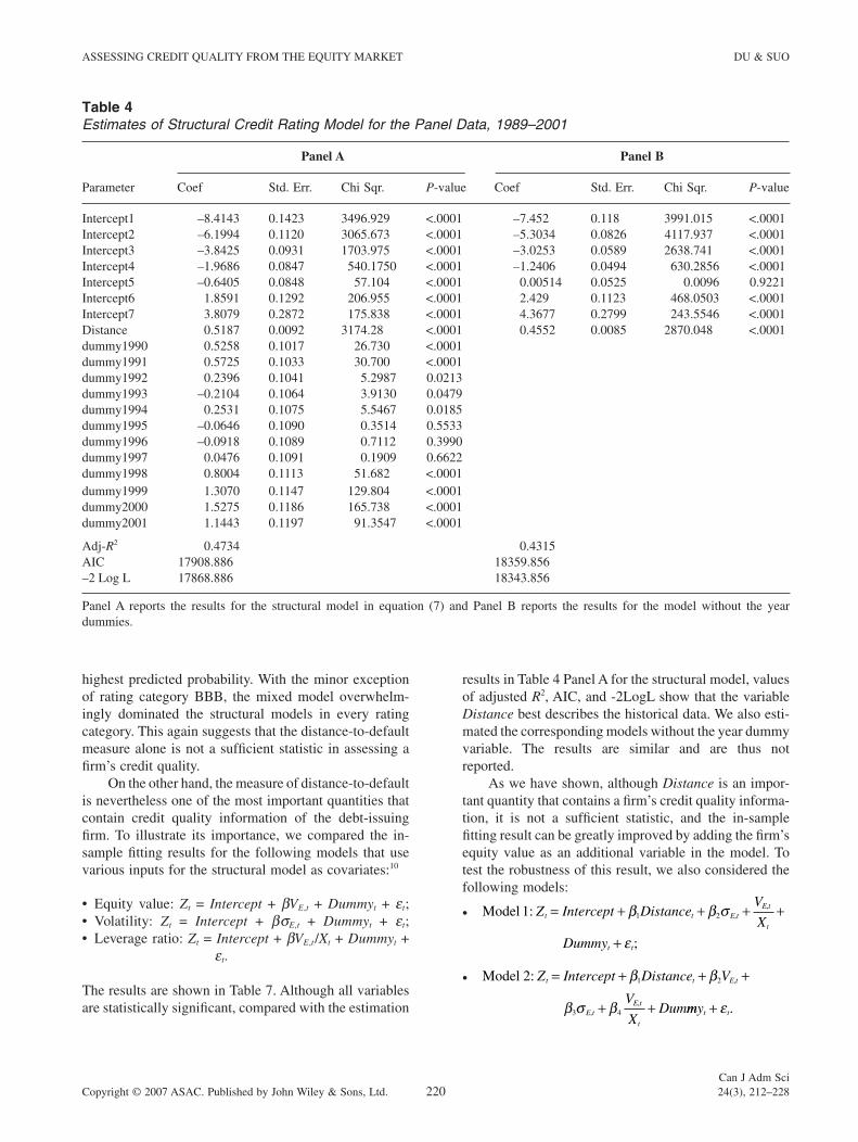
In order to show the empirical performance of the structural model, Table 4 Panel A presents the estimation results for the model specifi ed in equation (7). The struc-tural default probability measure, Distance, is statistically signifi cant. Moreover, the positive sign of the coeffi cient is consistent with the structural model prediction: the larger the distance-to-default, the less likely the fi rm will default. However, all three model fi tting measures – adjusted R2, AIC, and –2LogL – indicate that the model with the single independent variable Distance is not as good as traditional statistical models. Panel B presents the results when we omit the year dummy variable.

Table 2Correlation Matrix of Elements of Distance-to-Default

DistanceEquityValue

AssetValue

AssetVolatility

Distance 1Equity Value 0.42803 1Asset Value 0.32655 0.97742 1Asset Volatility –0.46275 –0.09422 –0.1038 1

This table presents the correlation matrix of distance, equity value, asset value, and asset volatility. In total, there are 6,635 fi rm-year observations.



Although structural models suggest that a fi rm’s credit quality is refl ected in the distance-to-default measure, the poor fi tting result suggests that this measure may not be adequate at refl ecting the market information concerning the debt-issuing fi rm’s credit quality. Results from Table 3 show that the fi rm’s equity value is a signifi cant factor affecting its credit quality besides its contribution to the equity-to-debt ratio.

To further illustrate this point, we investigated whether adding the equity value to the structural credit risk model could enhance the structural model’s fi tting ability. We constructed the following model:

Z Intercept Dis ce V Dummyt t E t t t= + + + +β β ε1 2tan , . (8)

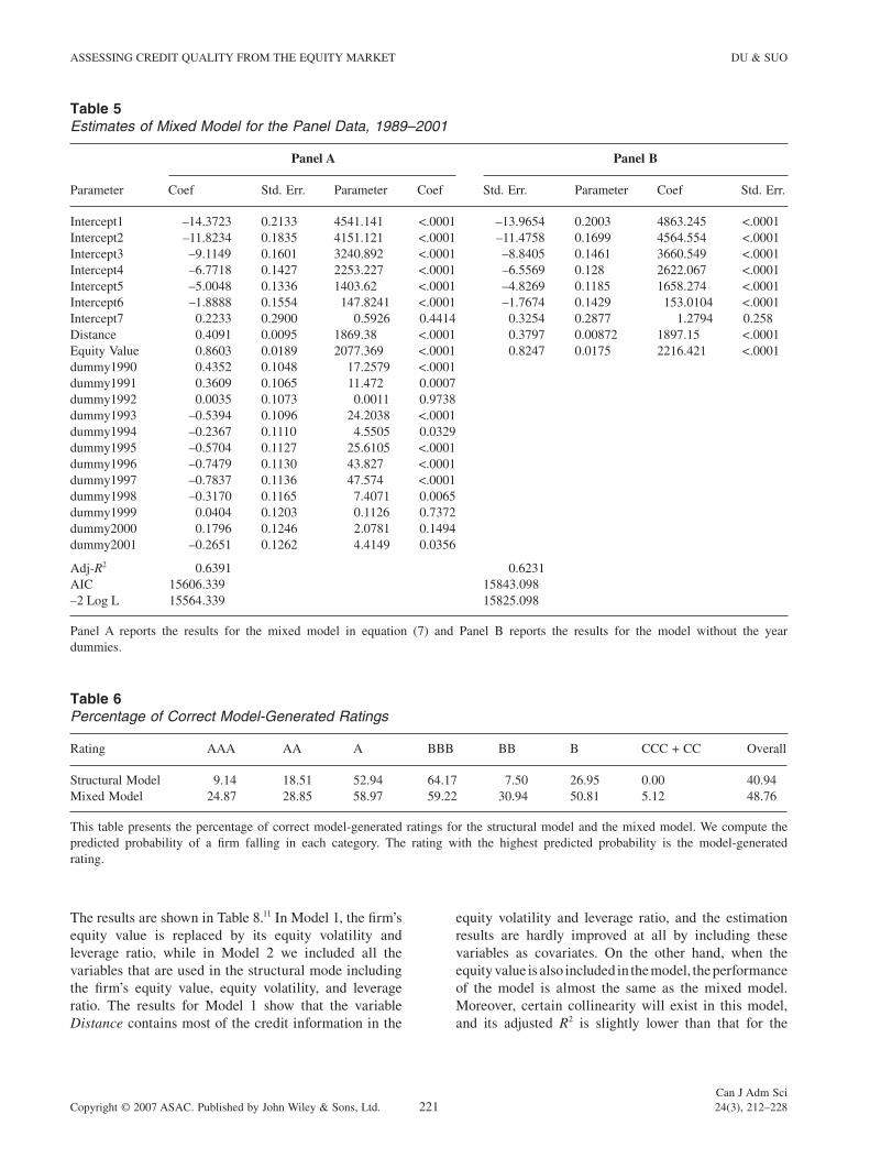
We refer to this as the mixed model.Table 5 Panel A provides estimation results for the

mixed model specifi ed in equation (8). In spite of its high correlation with the variable Distance as shown in Table

2, the fi rm’s equity value is still statistically signifi cant in explaining the fi rm’s credit quality. The values of adjusted R2, AIC, and –2LogL show that the mixed model performs best among the three models we consid-ered when fi tting the historical data. This suggests that contrary to the theoretical results from structural models, the Distance measure itself is not suffi cient in assessing a fi rm’s credit quality from the equity market information. Panel B reports similar results for the mixed model (8) without the year dummy variable.

To see if the models can correctly predict a fi rm’s credit rating, in Table 6 we show the percentage of correct rating predictions for each rating category. For brevity, we only compare the mixed model and the struc-tural model. Specifi cally, we computed the predicted probability of a fi rm falling in each category, and the model-generated rating was assigned as the most likely rating predicted by the models, that is, the one with the

Table 3Estimates of Statistical Credit Rating Model for the Panel Data, 1989–2001

Parameter

Panel A Panel B

Coef Std. Err. Chi Sqr. P-value Coef Std. Err. Chi Sqr. P-value

Intercept1 –10.0646 0.1966 2619.987 <.0001 –9.8087 0.1825 2888.041 <.0001Intercept2 –8.0049 0.1761 2067.187 <.0001 –7.7777 0.1609 2337.179 <.0001Intercept3 –5.5415 0.1596 1206.202 <.0001 –5.3524 0.1440 1381.873 <.0001Intercept4 –3.3158 0.1507 484.0935 <.0001 –3.1659 0.1350 549.8603 <.0001Intercept5 –1.3764 0.1515 82.5773 <.0001 –1.2588 0.1357 86.0138 <.0001Intercept6 2.9471 0.219 181.168 <.0001 2.9534 0.2021 213.5621 <.0001Intercept7 5.4128 0.3161 293.261 <.0001 5.3843 0.3036 314.4644 <.0001Equity Value 0.8151 0.0197 1714.453 <.0001 0.7791 0.0185 1764.703 <.0001Equity Volatility –15.1728 0.5173 860.2567 <.0001 –14.5622 0.4773 930.6691 <.0001Equity/Debt 0.7979 0.0338 556.0896 <.0001 0.7728 0.0335 532.0852 <.0001dummy1990 0.6196 0.1069 33.6177 <.0001dummy1991 0.3533 0.1079 10.7145 0.0011dummy1992 0.0843 0.1075 0.6145 0.4331dummy1993 –0.1326 0.1086 1.4915 0.2220dummy1994 –0.2259 0.1096 4.2466 0.0393dummy1995 –0.3077 0.1114 7.6286 0.0057dummy1996 –0.4074 0.1126 13.0817 0.0003dummy1997 –0.5212 0.1146 20.6882 <.0001dummy1998 –0.1209 0.119 1.0319 0.3097dummy1999 –0.00298 0.1222 0.0006 0.9805dummy2000 0.2143 0.1273 2.8352 0.0922dummy2001 –0.3066 0.128 5.7328 0.0167

Adj-R2 0.6221 0.6111AIC 15937.052 16085.999–2 Log L 15893.052 16065.999

These estimates are for the dynamic logistic model (6) and Panel B reports the results for the model without the year dummies.



highest predicted probability. With the minor exception of rating category BBB, the mixed model overwhelm-ingly dominated the structural models in every rating category. This again suggests that the distance-to-default measure alone is not a suffi cient statistic in assessing a fi rm’s credit quality.

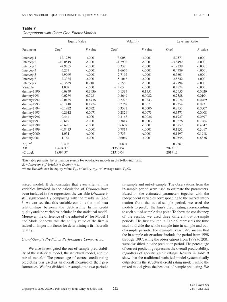
On the other hand, the measure of distance-to-default is nevertheless one of the most important quantities that contain credit quality information of the debt-issuing fi rm. To illustrate its importance, we compared the in-sample fi tting results for the following models that use various inputs for the structural model as covariates:10

• Equity value: Zt = Intercept + bVE,t + Dummyt + et;• Volatility: Zt = Intercept + bsE,t + Dummyt + et;• Leverage ratio: Zt = Intercept + bVE,t/Xt + Dummyt +

et.

The results are shown in Table 7. Although all variables are statistically signifi cant, compared with the estimation

results in Table 4 Panel A for the structural model, values of adjusted R2, AIC, and -2LogL show that the variable Distance best describes the historical data. We also esti-mated the corresponding models without the year dummy variable. The results are similar and are thus not reported.

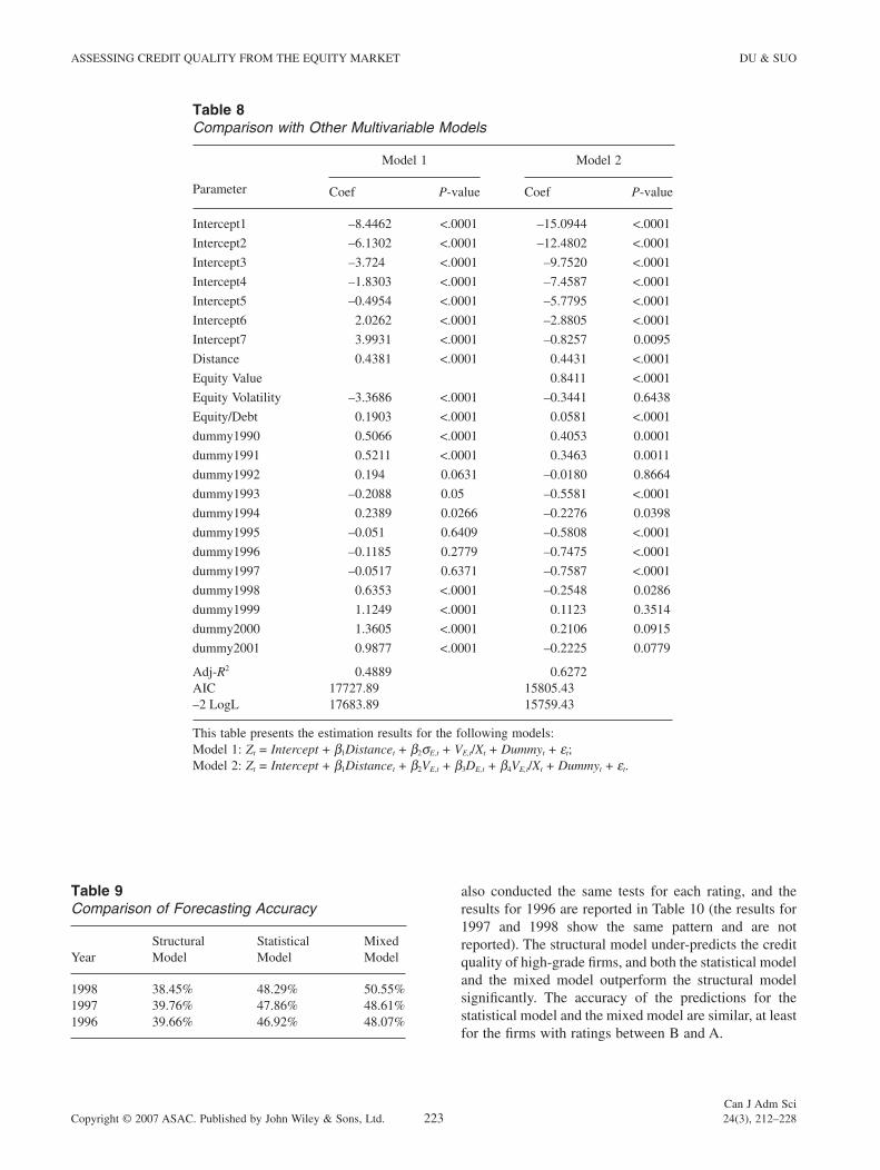
As we have shown, although Distance is an impor-tant quantity that contains a fi rm’s credit quality informa-tion, it is not a suffi cient statistic, and the in-sample fi tting result can be greatly improved by adding the fi rm’s equity value as an additional variable in the model. To test the robustness of this result, we also considered the following models:

• Model 1: ,,Z Intercept Dis ce

V

X

Dummy

t t E tE t

t

t t

= + + + +

+

β β σ

ε

1 2tan

;

• Model 2: ,

,,

Z Intercept Dis ce V

V

XDum

t t E t

E tE t

t

= + + +

+ +

β β

β σ β

1 2

3 4

tan

mmyt t+ ε .

Table 4Estimates of Structural Credit Rating Model for the Panel Data, 1989–2001

Parameter

Panel A Panel B

Coef Std. Err. Chi Sqr. P-value Coef Std. Err. Chi Sqr. P-value

Intercept1 –8.4143 0.1423 3496.929 <.0001 –7.452 0.118 3991.015 <.0001Intercept2 –6.1994 0.1120 3065.673 <.0001 –5.3034 0.0826 4117.937 <.0001Intercept3 –3.8425 0.0931 1703.975 <.0001 –3.0253 0.0589 2638.741 <.0001Intercept4 –1.9686 0.0847 540.1750 <.0001 –1.2406 0.0494 630.2856 <.0001Intercept5 –0.6405 0.0848 57.104 <.0001 0.00514 0.0525 0.0096 0.9221Intercept6 1.8591 0.1292 206.955 <.0001 2.429 0.1123 468.0503 <.0001Intercept7 3.8079 0.2872 175.838 <.0001 4.3677 0.2799 243.5546 <.0001Distance 0.5187 0.0092 3174.28 <.0001 0.4552 0.0085 2870.048 <.0001dummy1990 0.5258 0.1017 26.730 <.0001dummy1991 0.5725 0.1033 30.700 <.0001dummy1992 0.2396 0.1041 5.2987 0.0213dummy1993 –0.2104 0.1064 3.9130 0.0479dummy1994 0.2531 0.1075 5.5467 0.0185dummy1995 –0.0646 0.1090 0.3514 0.5533dummy1996 –0.0918 0.1089 0.7112 0.3990dummy1997 0.0476 0.1091 0.1909 0.6622dummy1998 0.8004 0.1113 51.682 <.0001dummy1999 1.3070 0.1147 129.804 <.0001dummy2000 1.5275 0.1186 165.738 <.0001dummy2001 1.1443 0.1197 91.3547 <.0001

Adj-R2 0.4734 0.4315AIC 17908.886 18359.856–2 Log L 17868.886 18343.856

Panel A reports the results for the structural model in equation (7) and Panel B reports the results for the model without the year dummies.



The results are shown in Table 8.11 In Model 1, the fi rm’s equity value is replaced by its equity volatility and leverage ratio, while in Model 2 we included all the variables that are used in the structural mode including the fi rm’s equity value, equity volatility, and leverage ratio. The results for Model 1 show that the variable Distance contains most of the credit information in the

equity volatility and leverage ratio, and the estimation results are hardly improved at all by including these variables as covariates. On the other hand, when the equity value is also included in the model, the performance of the model is almost the same as the mixed model. Moreover, certain collinearity will exist in this model, and its adjusted R2 is slightly lower than that for the

Table 5Estimates of Mixed Model for the Panel Data, 1989–2001

Parameter

Panel A Panel B

Coef Std. Err. Parameter Coef Std. Err. Parameter Coef Std. Err.

Intercept1 –14.3723 0.2133 4541.141 <.0001 –13.9654 0.2003 4863.245 <.0001Intercept2 –11.8234 0.1835 4151.121 <.0001 –11.4758 0.1699 4564.554 <.0001Intercept3 –9.1149 0.1601 3240.892 <.0001 –8.8405 0.1461 3660.549 <.0001Intercept4 –6.7718 0.1427 2253.227 <.0001 –6.5569 0.128 2622.067 <.0001Intercept5 –5.0048 0.1336 1403.62 <.0001 –4.8269 0.1185 1658.274 <.0001Intercept6 –1.8888 0.1554 147.8241 <.0001 –1.7674 0.1429 153.0104 <.0001Intercept7 0.2233 0.2900 0.5926 0.4414 0.3254 0.2877 1.2794 0.258Distance 0.4091 0.0095 1869.38 <.0001 0.3797 0.00872 1897.15 <.0001Equity Value 0.8603 0.0189 2077.369 <.0001 0.8247 0.0175 2216.421 <.0001dummy1990 0.4352 0.1048 17.2579 <.0001dummy1991 0.3609 0.1065 11.472 0.0007dummy1992 0.0035 0.1073 0.0011 0.9738dummy1993 –0.5394 0.1096 24.2038 <.0001dummy1994 –0.2367 0.1110 4.5505 0.0329dummy1995 –0.5704 0.1127 25.6105 <.0001dummy1996 –0.7479 0.1130 43.827 <.0001dummy1997 –0.7837 0.1136 47.574 <.0001dummy1998 –0.3170 0.1165 7.4071 0.0065dummy1999 0.0404 0.1203 0.1126 0.7372dummy2000 0.1796 0.1246 2.0781 0.1494dummy2001 –0.2651 0.1262 4.4149 0.0356

Adj-R2 0.6391 0.6231AIC 15606.339 15843.098–2 Log L 15564.339 15825.098

Panel A reports the results for the mixed model in equation (7) and Panel B reports the results for the model without the year dummies.

Table 6Percentage of Correct Model-Generated Ratings

Rating AAA AA A BBB BB B CCC + CC Overall

Structural Model 9.14 18.51 52.94 64.17 7.50 26.95 0.00 40.94Mixed Model 24.87 28.85 58.97 59.22 30.94 50.81 5.12 48.76

This table presents the percentage of correct model-generated ratings for the structural model and the mixed model. We compute the predicted probability of a fi rm falling in each category. The rating with the highest predicted probability is the model-generated rating.



mixed model. It demonstrates that even after all the variables involved in the calculation of Distance have been included in the regression, the variable Distance is still signifi cant. By comparing with the results in Table 3, we can see that this variable contains the nonlinear relationships between the debt-issuing fi rm’s credit quality and the variables included in the statistical model. Moreover, the difference of the adjusted R2 for Model 1 and Model 2 shows that the equity value of the fi rm is indeed an important factor for determining a fi rm’s credit quality.

Out-of-Sample Prediction Performance Comparisons

We also investigated the out-of-sample predictabil-ity of the statistical model, the structural model, and the mixed model.12 The percentage of correct credit rating predicting was used as an overall measure of their per-formances. We fi rst divided our sample into two periods:

in-sample and out-of-sample. The observations from the in-sample period were used to estimate the parameters. Based on the estimated parameters together with the independent variables corresponding to the market infor-mation from the out-of-sample period, we used the models to predict the fi rm’s credit rating corresponding to each out-of-sample data point. To show the consistency of the results, we used three different out-of-sample periods. The fi rst column in Table 9 represents the time used to divide the whole sample into in-sample and out-of-sample periods. For example, year 1998 means that the in-sample observations include the period from 1998 through 1997, while the observations from 1998 to 2001 were classifi ed into the prediction period. The percentage of correct predicting represents the overall predictability, regardless of specifi c credit ratings. Results in Table 9 show that the traditional statistical model systematically outperforms the structural credit rating model, while the mixed model gives the best out-of-sample predicting. We

Table 7Comparison with Other One-Factor Models

Parameter

Equity Value Volatility Leverage Ratio

Coef P-value Coef P-value Coef P-value

Intercept1 –12.1259 <.0001 –3.008 <.0001 –5.9571 <.0001Intercept2 –10.0519 <.0001 –1.2908 <.0001 –3.8492 <.0001Intercept3 –7.9765 <.0001 0.332 <.0001 –1.9238 <.0001Intercept4 –6.237 <.0001 1.6676 <.0001 –0.4789 <.0001Intercept5 –4.9049 <.0001 2.7197 <.0001 0.5801 <.0001Intercept6 –2.3385 <.0001 5.1046 <.0001 2.8642 <.0001Intercept7 –0.3659 0.218 7.158 <.0001 4.7794 <.0001Variable 1.007 <.0001 –14.65 <.0001 0.4574 <.0001dummy1990 0.0859 0.3936 0.1337 0.1751 0.2955 0.0029dummy1991 0.0269 0.7931 0.2649 0.0082 0.2588 0.0104dummy1992 –0.0435 0.6738 0.2276 0.0243 0.2024 0.0469dummy1993 –0.1418 0.1774 0.2769 0.007 0.2354 0.023dummy1994 –0.1922 0.0721 0.3572 0.0006 0.3551 0.0007dummy1995 –0.2912 0.0071 0.2829 0.0073 0.3571 0.0008dummy1996 –0.4441 <.0001 0.3168 0.0026 0.1927 0.0697dummy1997 –0.619 <.0001 0.3817 0.0003 0.0276 0.7964dummy1998 –0.696 <.0001 0.6607 <.0001 0.0852 0.4347dummy1999 –0.8433 <.0001 0.7817 <.0001 0.1152 0.3017dummy2000 –1.0311 <.0001 0.735 <.0001 0.1497 0.1918dummy2001 –1.164 <.0001 0.6069 <.0001 0.0555 0.6336

Adj-R2 0.4081 0.0894 0.2367AIC 18634.37 21350.04 20231.3–2 LogL 18594.37 21310.04 20191.3

This table presents the estimation results for one-factor models in the following form:Zt = Intercept + bVariablet + Dummyt + et,where Variable can be equity value VE,t, volatility sE,t, or leverage ratio VE,t/Xt.



Table 8Comparison with Other Multivariable Models

Model 1 Model 2

Parameter Coef P-value Coef P-value

Intercept1 –8.4462 <.0001 –15.0944 <.0001

Intercept2 –6.1302 <.0001 –12.4802 <.0001

Intercept3 –3.724 <.0001 –9.7520 <.0001

Intercept4 –1.8303 <.0001 –7.4587 <.0001

Intercept5 –0.4954 <.0001 –5.7795 <.0001

Intercept6 2.0262 <.0001 –2.8805 <.0001

Intercept7 3.9931 <.0001 –0.8257 0.0095

Distance 0.4381 <.0001 0.4431 <.0001

Equity Value 0.8411 <.0001

Equity Volatility –3.3686 <.0001 –0.3441 0.6438

Equity/Debt 0.1903 <.0001 0.0581 <.0001

dummy1990 0.5066 <.0001 0.4053 0.0001

dummy1991 0.5211 <.0001 0.3463 0.0011

dummy1992 0.194 0.0631 –0.0180 0.8664

dummy1993 –0.2088 0.05 –0.5581 <.0001

dummy1994 0.2389 0.0266 –0.2276 0.0398

dummy1995 –0.051 0.6409 –0.5808 <.0001

dummy1996 –0.1185 0.2779 –0.7475 <.0001

dummy1997 –0.0517 0.6371 –0.7587 <.0001

dummy1998 0.6353 <.0001 –0.2548 0.0286

dummy1999 1.1249 <.0001 0.1123 0.3514

dummy2000 1.3605 <.0001 0.2106 0.0915

dummy2001 0.9877 <.0001 –0.2225 0.0779

Adj-R2 0.4889 0.6272AIC 17727.89 15805.43–2 LogL 17683.89 15759.43

This table presents the estimation results for the following models:Model 1: Zt = Intercept + b1Distancet + b2sE,t + VE,t/Xt + Dummyt + et;Model 2: Zt = Intercept + b1Distancet + b2VE,t + b3DE,t + b4VE,t/Xt + Dummyt + et.

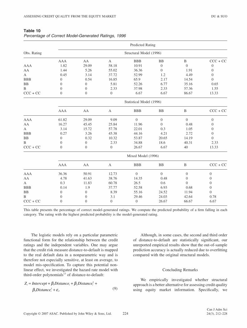
also conducted the same tests for each rating, and the results for 1996 are reported in Table 10 (the results for 1997 and 1998 show the same pattern and are not reported). The structural model under-predicts the credit quality of high-grade fi rms, and both the statistical model and the mixed model outperform the structural model signifi cantly. The accuracy of the predictions for the statistical model and the mixed model are similar, at least for the fi rms with ratings between B and A.

Table 9Comparison of Forecasting Accuracy

YearStructuralModel

StatisticalModel

MixedModel

1998 38.45% 48.29% 50.55%1997 39.76% 47.86% 48.61%1996 39.66% 46.92% 48.07%



The logistic models rely on a particular parametric functional form for the relationship between the credit ratings and the independent variables. One may argue that the credit risk measure distance-to-default is mapped to the real default data in a nonparametric way and is therefore not especially sensitive, at least on average, to model mis-specifi cation. To capture this potential non-linear effect, we investigated the hazard rate model with third-order polynomials13 of distance-to-default:

Z Intercept Dis ce Dis ce

Dis cet t t

t t

= + + ++

β ββ ε

1 22

33

tan tan

tan .

(9)

Although, in some cases, the second and third order of distance-to-default are statistically signifi cant, our unreported empirical results show that the out-of-sample prediction accuracy is actually reduced due to overfi tting compared with the original structural models.

Concluding Remarks

We empirically investigated whether structural approach is a better alternative for assessing credit quality using equity market information. Specifi cally, we

Table 10Percentage of Correct Model-Generated Ratings, 1996

Obs. Rating

Predicted Rating

Structural Model (1996)

AAA AA A BBB BB B CCC + CCAAA 1.82 29.09 58.18 10.91 0 0 0AA 1.44 5.26 55.02 36.36 0 1.91 0A 0.45 3.14 37.72 52.99 1.2 4.49 0BBB 0 0.54 16.85 65.9 2.17 14.54 0BB 0 0 5.81 52.26 6.77 35.16 0.65B 0 0 2.33 37.98 2.33 57.36 1.55CCC + CC 0 0 0 6.67 6.67 86.67 13.33

Statistical Model (1996)

AAA AA A BBB BB B CCC + CC

AAA 61.82 29.09 9.09 0 0 0 0AA 16.27 45.45 25.84 11.96 0 0.48 0A 3.14 15.72 57.78 22.01 0.3 1.05 0BBB 0.27 3.26 45.38 44.16 4.21 2.72 0BB 0 0.32 10.32 53.87 20.65 14.19 0B 0 0 2.33 34.88 18.6 40.31 2.33CCC + CC 0 0 0 26.67 6.67 40 13.33

Mixed Model (1996)

AAA AA A BBB BB B CCC + CC

AAA 36.36 50.91 12.73 0 0 0 0AA 4.78 41.63 38.76 14.35 0.48 0 0A 0.3 11.83 60.78 26.5 0.6 0 0BBB 0.14 1.9 37.77 52.58 6.93 0.68 0BB 0 0 8.39 55.16 24.52 11.94 0B 0 0 3.1 29.46 24.03 42.64 0.78CCC + CC 0 0 0 0 26.67 66.67 6.67

This table presents the percentage of correct model-generated ratings. We compute the predicted probability of a fi rm falling in each category. The rating with the highest predicted probability is the model-generated rating.



investigated whether the credit risk measure from the structural models is adequate at refl ecting the market information contained in the variables in the model. Both in-sample fi tting and out-of-sample prediction showed that the structural credit risk model does not generate a suffi cient statistic of the market information concerning credit quality. For example, we found that the empirical performance of in-sample fi tting and out-of-sample pre-diction of the model can be greatly improved by adding the equity value to the model. In other words, credit quality information contained in the equity value of the fi rm is not fully utilized by structural credit risk models. For this reason, it seems that structural credit risk models, although theoretically appealing, should be used with caution when assessing a fi rm’s credit quality.

Although our results showed that the structural model has diffi culty in capturing credit risk, they provide indirect support to the conclusion of Huang and Huang (2003) that credit risk accounts for only a fraction of the observed credit spread, especially for investment grade bonds. Specifi cally, by missing equity value, which is negatively correlated with default probability, they obtained a default probability measure biased upward for investment-grade fi rms whose equity size is large. Hence, the model credit spreads would be larger than what can be justifi ed by the actual default probabilities. Yet even this larger model spread is only a fraction of the actual spreads observed in the market. On the contrary, our results suggest that structural models are not able to suf-fi ciently capture and price credit risk. Our results are also consistent with the fi ndings of Eom et al. (2004), who systematically examine fi ve structural credit risk models14 and fi nd that all of them have diffi culties in accurately forecasting credit spreads.

Implications for Theory and Practice

Our results are relevant to both researchers and prac-titioners in fi nance. Recent studies concerning the credit risk, such as Vassalou and Xing (2003, 2004), often used the measure of distance-to-default derived from the Merton model as a proxy for the debt-issuing fi rm’s credit quality. Moreover, the newly adopted Basel II specifi cally requires fi nancial institutions to implement models to adequately measure the default risk of their portfolios. Our results suggest that the distance-to-default measure from the Merton model should be used with caution because it does not adequately refl ect all the credit quality information contained in the variables involved in constructing the measure.

Limitations and Directions for Future Research

Finally, our conclusions are based on the assumption that credit rating is an accurate and timely measure of credit quality. It is, however, possible that the Merton type of models do refl ect the actual default probability of each fi rm, yet the credit ratings assigned by rating agencies do not suffi ciently refl ect a fi rm’s credit quality15 or credit ratings do not refl ect a fi rm’s fi nancial health in a timely way. As a result, KMV’s measure is not able to predict the credit rating very well. Moreover, we only studied the Merton model, and it would be interesting to see whether other more complicated structural models, such as Leland and Toft (1996) and Collins-Dufresne and Goldstein (2001), can adequately refl ect the credit default risk of the debt-issuing fi rm.

Notes

1 The drift term mA – s 2A/2 for the logarithm of the asset value is usually ignored in the defi nition of distance-to-default. However, the resulting value will be very close since the model is often used for a one-year time horizon, and the drift term is very small.

2 There are two main differences between Vassalou and Xing (2004) and KMV. KMV uses a more complicated method to assess the asset volatility than Vassalou and Xing, which incorporates Bayesian adjustments for the country, industry, and size of the fi rm. KMV also allows for convertibles and preferred stocks in the capital struc-ture of the fi rm, whereas Vassalou and Xing allow only equity, as well as short- and long-term debt. In this study, we follow the Vassalou and Xing approach.

3 Our tolerance level for convergence is 2 × 10E – 4. 4 This approach was originally proposed by Ronn and

Verma (1986). The parameters in the structural model can also be estimated by using the maximum likelihood esti-mation; see Duan (1994) and Ericsson and Reneby (2005) for discussions.

5 KMV has a proprietary default database including more than 250,000 fi rm-years observations and more than 4,700 incidents of default or bankruptcy. It has a procedure to map the distance-to-default to the empirical data and calculate the expected default frequency.

6 Following conventions of the literature, we take the loga-rithm of the equity value.

7 Because of the aging effect documented by Altman (1989), we do not include newly rated fi rms after 1988 into our sample (i.e., newly rated fi rms and seasoned fi rms have different rating transition probability).

8 Some fi rms may drop from our sample before 2001, either because of default or because of their ratings being withdrawn. For example, if a fi rm defaulted in, say, 1993, then that fi rm will be deleted from the sample since 1993. In other words, only the observations of that fi rm over the period of 1988 to 1992 will be included in the sample.

9 We truncate the estimated asset value volatility at the end of each iteration.



10 We thank the referee for this suggestion.11 To save space, we omit the standard errors and Chi-square

values of the estimations.12 We have also considered the forecasting performance for

the model in equation (9). The results are very similar to the case of the mixed model.

13 The authors thank Frank Zhang of Moody’s KMV for this suggestion.

14 The models studied include Merton (1974), Leland and Toft (1996), Longstaff and Schwartz (1995), and Collin-Dufresne and Goldstein (2001).

15 The authors thank Professors Darrell Duffi e and Frank Milne for their comments on this point.

16 A cycle begins when the fi rm enters a new credit rating and ends when it migrates to another rating

References

Altman, E. (1989). Measuring Corporate Bond Mortality and Performance. Journal of Finance, 44, 909–922.

Benos, A., & Papanastasopoulos, G. (2005). Extending the Merton Model: A Hybrid Approach to Assessing Credit Quality. Manuscript in preparation, University of Piraeus, Piraeus, Greece.

Bharath, S., & Shumway, T. (2004). Forecasting Default with the KMV-Merton Model. Manuscript in preparation, Ross School of Business, University of Michigan.

Blume, M., Lim, R., & MacKinlay, A.C. (1998). The Declining Credit Quality of U.S. Corporate Debt: Myth or Reality? Journal of Finance, 4, 1389–1413.

Collin-Dufresne, P. & Goldstein, R. (2001). Do Credit Spreads, Refl ect Stationary Leverage Ratio? Journal of Finance, 56, 1929–1957.

Du, Y. (2003). Predicting Credit Rating and Credit Rating Changes: A New Approach. Manuscript in preparation, Queen’s School of Business, Queen’s University, Canada.

Duan, J.-C. (1994). Maximum Likelihood Estimation Using Price Data of the Derivative Contract. Mathematical Finance, 4, 155–167.

Duffi e, D., & Lando, D. (2001). Term Structure of Credit Spread with Incomplete Information. Econometrica, 69, 155–180.

Eom, Y., Helwege, J., & Huang, J. (2004). Structural Models of Corporate Bond Pricing: An Empirical Analysis, Review of Financial Studies, 17, 499–544.

Ericsson, J., & Reneby, J. (2005). Estimating Structural Bond Pricing Models. Journal of Business, 78, 707–735.

Ericsson, J., & Renault, O. (2006). Liquidity and Credit Risk. Journal of Finance, 61, 2219–2250.

Fama, E., & French, K. (1996). Multifactor Explanations of Asset Pricing Anomalies. Journal of Finance, 51, 55–84.

Geske, R., & Delianedis, G. (1998). Credit Risk and Risk Neutral Default Probabilities: Information about Rating Migrations and Defaults. Manuscript in preparation. Anderson School of Management, University of California, LA.

Gourieroux, C. (2000). Econometrics of Qualitative Dependent Variables. Cambridge University Press: Cambridge, UK.

Hillegeist, S., Keating, E.K., Cram, D.P., & Lundstedt, K.G. (2004). Assessing the Probability of Bankruptcy. Review of Accounting Studies, 9, 5–34.

Horrigan, J.O. (1966). The Determination of Long-term Credit Standing with Financial Ratios. Journal of Accounting Research, 4(supp.), 44–62.

Huang, M., & Huang, J. (2003). How Much of the Corporate-Treasury Yield Spread is Due to Credit Risk? Manuscript in preparation, Graduate School of Business, Stanford University, Stanford, CA.

Hull, J., & White, A. (1995). The Impact of Default Risk on the Valuation of Options and Other Derivative Securities. Journal of Banking and Finance, 19, 299–322.

Kaplan, R., & Urwitz, G. (1979). Statistical Models of Bond Ratings: A Methodological Inquiry. Journal of Business, 52, 231–261.

KMV Corporation. (1998). Uses and Abuses of Bond Default Rates. Research paper, San Francisco, CA.

KMV Corporation. (2002). Modeling Default Risk. Research paper, San Francisco, CA.

Lancaster, T. (1990). The Econometric Analysis of Transition Data. Cambridge University Press: New York, NY.

Leland, H. (1998). Agency Costs, Risk Management, and Capital Structure. Journal of Finance, 53, 1213–1243.

Leland, H. (2002). Predictions of Expected Default Frequen-cies in Structural Models of Debt. Manuscript in prepara-tion, The Hass School of Business, University of California, Berkeley.

Leland, H., & Toft, K. (1996). Optimal Capital Structure, Endogenous Bankruptcy, and the Term Structure of Credit Spreads. Journal of Finance, 51, 987–1019.

Longstaff, F., & Schwartz, E.S. (1995). A Simple Approach to Valuing Risky Fixed and Floating Rate Debt. Journal of Finance, 50, 789–819.

Merton, R. (1974). On the Pricing of Corporate Debt: The Risk Structure of Interest Rates. Journal of Finance, 29, 449–470.

Ohlson, J. (1980). Financial Ratios and the Probabilistic Predic-tion of Bankruptcy. Journal of Accounting Research, 19, 109–131.

Pogue, T., & Soldofsky, R. (1969). What is in a Bond Rating? Journal of Financial and Quantitative Analysis, 4, 210–228.

Ronn, E., & Verma, A. (1986). Pricing Risk-adjusted Deposit Insurance: An Option Based Model. Journal of Finance, 41, 871–895.

Shumway, T. (2001). Forecasting Bankruptcy More Accu-rately: A Simple Hazard Rate Model. Journal of Business, 74, 101–124.

Vassalou, M., & Xing, Y. (2003). Equity Returns Following Changes in Default Risk: New Insights into the Informational Content of Credit Ratings. Manuscript in preparation, Graduate School of Business, Columbia University.

Vassalou, M., & Xing, Y. (2004). Default Risk in Equity Returns. Journal of Finance, 59, 831–868.



West, R. (1973). Bond Ratings, Bond Yields and Financial Regulations: Some Findings. Journal of Law and Eco-nomics, 16, 159–168.

Appendix

Estimating Hazard Rate Models

We assume that credit rating migration can happen at any of the following discrete times, t = t0 + ∆s, t0 + 2∆s, . . . , where ∆s can be very small to approximate the continuous time setting. We use Ti to represent the time when fi rm i leaves our sample (for ease of notation, we omit the subscript i).

Let the probability of transition from credit rating l to rating m at time t + s be given by plm(t,x,s), where s measures the duration that rating l has been continuously occupied since it was entered at time t and x represents the independent variables, or the covariates, which can be time-varying.

Let qlm(t,x,s) represent the transition intensity from rating l to rating m, given that state l was entered at time t and has been occupied up to time t + s. The variable qlm(t,x,s)∆s represents the probability at time t that a departure from rating l to state m occurs during the time interval from t + s to t + s + ∆s. This probability is con-ditional on the rating l being occupied for s period of time since t, and upon the previous transition history. Furthermore, we let c denote the c’th cycle16 of the rating migrations process, with the total number of cycles being C. In addition, we let Sc be the duration of the c’th cycle. We assume that rating migration only occurs at the end of each cycle. We also defi ne a binary indicator dcm, which equals 1 if rating m is entered at the end of the c’th cycle, and 0 otherwise.

Proof of the Equivalence

Shumway’s (2001) model is the simplest hazard rate model. Specifi cally, there are only two states in his model: default and not default. Furthermore, if a fi rm defaults, it will be removed from the data sample only after the default occurs. Shumway’s (2001) model is a binary, single-cycle hazard rate model. This model is suffi cient for studying bankruptcy events. For credit rating, however, each fi rm has multiple possible destina-tions when it experiences a rating change. For example, its rating can transfer from AAA to AA, or BB, or CC, or even default. In addition, each fi rm can experience multiple rating migrations during a particular period of time. In this Appendix, we show that Shumway’s (2001)

approach can be extended to the multinomial, multipe-riod case and demonstrate the equivalence of the hazard rate model and the dynamic logistic model. Equivalence refers to their likelihood functions and estimates being identical.

Proposition: A multiperiod, multinomial logistic model is equivalent to a hazard rate model with hazard function Plm(t,x,s)/∆s.

Proof: A multiperiod, multinomial logistic model is estimated with each panel data point, say each fi rm-year, as if it were a separate observation. The contribution of a specifi c fi rm i to the likelihood function during its cycle in the sample is given as follows:

l P t x s P t x Sll c cs

S d

lm c cm

K d d

c

c c l c m c

= ( )

( )= =

∏ ∏− −

, , , ,, ,

0 1

1 1,,

,

l

l

K

c

C

l m

≠==

∏ ;11�

(10)

where Sc is the completed duration of cycle c and tc is the calendar time at which the c’th cycle was commenced. Credit rating changes only happen at the end of each cycle after a rating was entered.

Equation (10) is intuitive. In its life cycle, a fi rm could transit within all possible credit rating states, including the bankrupt state, or stay in its original rating. The likelihood contributed by any specifi c fi rm is the product of the transition probabilities and/or the proba-bility of staying in its original rating. For example, suppose a fi rm’s rating at time t0 was AAA, then time t0 + ∆s was downgraded to AA, then time t0 + 2∆s down-graded to B, where it remained. The likelihood function contributed by this fi rm is PAAA,AA(·)PAA,B(·)PB,B(·). An implicit assumption made here is that the latent variable solely determines the credit rating migration probability.

Because ∆s is a constant, we can divide equation (10) by polynomials of ∆s without changing the maximum likelihood estimation results. Then we have:

′ = ( )

( )

=

∏−

l P t x sP t x S

sll c c

s

S d l

lm c cd

c

c c c m

, ,, ,

, ,

0

1

∆

dd

m

K

l

K

c

C c l

l m

−

===∏∏

≠

1

111

,

;�

.

(11)

We get the following log likelihood function:

L d dP t x S

s

d

c l c mlm c c

m

K

l

K

c

C

c

= ( )

+ −

===

−

∑∑∑ 1111

1

, , log, ,

∆

,, log , , ,l ll c cs

S

P t x s l mc

c

( ) ≠=

∏0

.

(12)



Let Plm(tc,x,sc) = θlm(tc,x,sc)∆s. Recall that for l ≠ m (see Gourieroux (2000)),

P t x s t x u dulls

S

c c lmm

KS

c

c

c c

= =∏ ∑∫( ) ≈ − ( )

0 10

, exp , ,, .θ (13)

Then we arrive:

L d d t x S

d

m

K

c l c m lm c cl

K

c

C

c l

S

m

c

= ( ) − =

−==

−=

∑∑∑

∫

11

11

1

0 1

, ,

,

log , ,θ

KK

lm ct x u du l m∑ ( )

≠θ , , , .

(14)

Rearranging the terms, we have:

L d d t x S z t x Sc

C

l

K

m

K

c l c m lm c c lm c c= ( ) − ( )[ ]= = =

−∑∑∑1 1 1

1, , log , , , , ,θ (15)

where

z t x S t x u dulm c c

S

m

K

lm c

c

, , , ,( ) = ( )∫∑=0 1

θ .

Equation (15) is exactly the likelihood function for the multiperiod, multinomial hazard rate model discussed

in Lancaster (1990). Therefore, if we let the probability density function of transition from credit rating l to rating m be given by Plm/∆s, the likelihood function of a multi-period logistic model is equivalent to the likelihood func-tion of a discrete-time hazard rate model.

Inference of Hazard Rate Models

Making statistical inferences in a hazard model esti-mated with a logistic program is straightforward. Since the dynamic logistic and hazard models have the same likelihood function, they have the same asymptotic cova-riance matrix. The c2 test statistics provided by the logis-tic program take the following form:

ˆ ˆ ~µ µ µ µ χk k k−( )′ −( ) ( )−0

10

2Σ , (16)

where there are k estimated moments being tested against k null hypotheses m0 and S is the estimated covariance matrix.

Assessing credit quality from the equity market: can a structural approach forecast credit ratings?

Documents

Transcript of Assessing credit quality from the equity market: can a structural approach forecast credit ratings?