Assembly and Employment

of a Microphone Array with a Text-Independent

Speaker Identification System

J O N A S N A H L I N

Master of Science Thesis Stockholm, Sweden 2007

Assembly and Employment

of a Microphone Array with a Text-Independent

Speaker Identification System

J O N A S N A H L I N

Master’s Thesis in Speech Communication (20 credits) at the School of Media Technology Royal Institute of Technology year 2007 Supervisors at CSC were Daniel Elenius and Mats Blomberg Examiner was Björn Granström TRITA-CSC-E 2007:076 ISRN-KTH/CSC/E--07/076--SE ISSN-1653-5715 Royal Institute of Technology School of Computer Science and Communication KTH CSC SE-100 44 Stockholm, Sweden URL: www.csc.kth.se

Abstract In this Master thesis, the combination of a 64 sensor microphone array named MarkIII/IRST-Light and a text-independent speaker identification system is investigated. The work is carried out within the EU-funded CHIL project (Computers in the Human Interaction Loop) for which the research of unobtrusive technology is a main focus. By exploiting the spatial correlation of the multiple signals produced by microphone array sensors, speech signal enhancement can be achieved. One technique for this signal processing is known as beamforming. No operational beamformer could be set up within the scope of this project. However, the effort put into the preparation of the MarkIII should provide the basis for further attempts to set up beamforming at the Department of Speech, Music and Hearing (TMH). The speaker identification system is developed mainly using tools of HTK, which is a toolkit for building HMMs. The process is divided into two steps: Firstly, a speaker-independent background model is trained using speech data from the SpeeCon database. Secondly, data collected from ten Swedish speakers is used to derive ten speaker-dependent models through MAP adaptation. Two different speaker model designs are employed: The single GMM approach and a design where multiple states are tied to share the same output distribution. Results indicate that the multi-tied-state design performs better than the single GMM approach. Another outcome of the project is the carried out assembly of the MarkIII.

Iordningställning och användning av en mikrofonarray i ett textoberoende talaridentifieringssystem

Sammanfattning I detta examensarbete studeras kombinationen av en mikrofonarray och ett system för textoberoende talaridentifiering. Mikrofonarrayen, som används för att göra ljudinspelningar med 64 kanaler, går under namnet MarkIII/IRST-Light. Projektet är underordnat det EU-finansierade projektet CHIL (Computers in the Human Interaction Loop) som inriktar sig på forskning inom så kallad ”unobtrusive technology”. Detta begrepp åsyftar teknik som stödjer mänskliga aktiviteter utan att dess närvaro kräver uppmärksamhet från de personer som är involverade i det aktuella skeendet. Genom att utnyttja den korrelation som uppstår när en mikrofonarray används för samtidig inspelning över ett flertal kanaler, kan uppfattbarheten av en talsignal ökas. En teknik för att åstadkomma detta kallas beamforming. Implementation av en beamforming-algoritm kunde inte genomföras inom ramen för detta examensarbete, men det arbete som lagts ned på att förbereda mikrofonarrayen för användning bör kunna utgöra en god förutsättning för fortsatt arbete med beamforming på TMH (Instutitionen för Tal, Musik och Hörsel). För utformandet av talaridentifikationssystemet används i första hand HTK som är ett toolkit som används för att skapa HMMer. Förloppet delas upp i två faser: Inledningsvis tränas en talaroberoende bakgrundsmodell med data som hämtas från taldatabasen SpeeCon. I fas två spelas taldata in från tio svenska talare och används för MAP-adaption av den ursprungliga modellen. Denna process leder till tio nya talarberoende modeller. Två olika modellstrukturer används i systemet: Den första består endast av en GMM. Den andra modellen byggs upp av ett flertal tillstånd (states) som alla delar samma pdf (proablilty desity function). Denna pdf definieras av en GMM. Utvärdering av de båda modellstrukturerna visar bäst identifikationsresultat för flerstates-modellen. Ett praktiskt resultat av projektet utgörs av den iordningställda mikrofonarrayen.

Table of Contents CHAPTER 1: INTRODUCTION...........................................................................................................................1

1.1 BACKGROUND ..............................................................................................................................................1 1.1.1 Starting Point of Thesis..........................................................................................................................1

1.2 THESIS OBJECTIVE .......................................................................................................................................3 1.3 PAPER OUTLINE ...........................................................................................................................................3

CHAPTER 2: THEORY ..........................................................................................................................................5 2.1 MICROPHONE ARRAYS ................................................................................................................................5

2.1.1 Beamforming..........................................................................................................................................5 2.1.2 Sound Source Localization ....................................................................................................................6

2.2 AUTOMATIC SPEAKER IDENTIFICATION......................................................................................................7 2.2.1 Speaker Recognition ..............................................................................................................................7

2.2.1.1 Speech Signal Representation in Recognition Systems ............................................................................. 8 2.2.2 The Hidden Markov Model ...................................................................................................................9

2.2.2.1 The Markov Chain...................................................................................................................................... 10 2.2.2.2 Extension to HMM ..................................................................................................................................... 10 2.2.2.3 Parameter Tying.......................................................................................................................................... 11 2.2.2.4 Efficient Modeling for Text-Independent Speaker Identification ........................................................... 12 2.2.2.5 Adaptation ................................................................................................................................................... 12

CHAPTER 3: EXPERIMENT METHOD..........................................................................................................15 3.1 SETTING UP THE MARKIII/IRST-LIGHT MICROPHONE ARRAY ..............................................................15

3.1.1 Assembly of the MarkIII Hardware ....................................................................................................15 3.1.2 Smartflow .............................................................................................................................................16 3.1.3 Attempts to Set Up Beamforming.......................................................................................................17

3.2 IMPLEMENTATION OF THE SPEAKER IDENTIFICATION SYSTEM ...............................................................18 3.2.1 Creating the Universal Background Model (UBM)...........................................................................19

3.2.1.1 Training Data Acquisition.......................................................................................................................... 19 3.2.1.2 Training Data Parameterization ................................................................................................................. 19 3.2.1.3 Training the Background Model................................................................................................................ 20

3.2.2 Data Collection for Adaptation and Testing.......................................................................................21 3.2.2.1 Manual Processing of the Collected Speech Data .................................................................................... 22

3.2.3 Parameterization of the MarkIII data ..................................................................................................23 3.2.4 Adaptation.............................................................................................................................................24

3.3 ASSESSMENT OF THE SPEAKER IDENTIFICATION SYSTEM .......................................................................25 3.3.1 Recognition...........................................................................................................................................25 3.3.2 Evaluation .............................................................................................................................................26

CHAPTER 4: RESULTS .......................................................................................................................................27 CHAPTER 5: DISCUSSION.................................................................................................................................31

5.1 WORKING WITH THE MARKIII...................................................................................................................31 5.2 REFLECTIONS REGARDING THE IDENTIFICATION RESULTS .....................................................................31

5.2.1 Amount of Adaptation Data ................................................................................................................32 5.2.2 Robustness of the Speaker Identification System ..............................................................................32

CHAPTER 6: CONCLUSIONS ...........................................................................................................................33 CHAPTER 7: FUTURE WORK ..........................................................................................................................35 REFERENCES ............................................................................................................................................................37 APPENDIX A: PROMPTS FOR SPEECH DATA ACQUISITION..................................................................41 APPENDIX B: PHOTOGRAPHS OF THE MARKIII ........................................................................................43

Acknowledgments I would like to thank my supervisors Daniel Elenius and Mats Blomberg for their valuable support during the work with this Master thesis. During the project I have also received helpful assistance from Håkan Melin, Kjell Elenius and Rolf Carlson at TMH. Thank you! This thesis would not have come about had not Björn Granström invited me to work on this project at TMH. I am also grateful to Kent Lindgren at the Wallenbergslaboratoriet who helped me with the precision work of constructing the box for the MarkIII/IRST-Light microphone array. Furthermore, John McDonough, Cedrick Rochet, Uwe Maier, Szeder Gábor and Tobias Gehrig at ISL in Karlsruhe have been more than helpful during the process of setting up the microphone array. My thanks also go out to the photographer Anna Piggelina Sundström who provided the photo documentation of the assembled microphone array. Finally, I would like to thank the ten subjects who provided the speech data used in the speaker identification experiment.

List of Abbreviations CHIL Computers in the Human Interaction Loop DOA Direction Of Arrival FFT Fast Fourier Transform GMM Gaussian Mixture Model HMM Hidden Markov Model HTK Hidden Markov model Toolkit ISL Interactive Systems Labs (University of Karlsruhe) MAP Maxiumum A-Posteriori MFCC Mel Frequency Cepstral Coefficients MLLR Maxiumum Likelihood Linear Regression NIST National Institute of Standards and Technology pdf Probability Density Function SNR Signal Noise Ratio TA Targeted Audio TMH Department of Speech, Music and Hearing (KTH) UBM Universal Background Model

1

Chapter 1: Introduction

1.1 Background In society of today the demand for fast and efficient communication is increasing. This demand needs to be met by the development and refinement of techniques with the aim to facilitate the flow of information and to support communication between interacting persons. As of today technical solutions are employed to support human interaction through video conferencing, audio conferencing, hands-free telephony and so on. As such techniques are further employed, the demand for functionality and usability grows. A common problem in this setting is that the presence of computers and other technical aids will require attention from the interacting parties. Thereby the technology itself draws focus from the task at hand, impeding the communication it is supposed to support. Hence an important step to further facilitate communication between humans may be the development of techniques which support human interaction without requiring the interacting parties to be preoccupied with the technology itself. Such unobtrusive technologies are examined and developed within an EU-funded project by the name of CHIL1 (Computers in the Human Interaction Loop) and it is within the CHIL framework this Master thesis work has been carried out. The CHIL project is set to have a 44 month duration and was launched on January, 1st 2004. It is jointly coordinated by the University of Karlsruhe and the Fraunhofer Institute (IITB). The overall goal of the CHIL project is to make everyday life easier through the creation of environments with the ability to aid human interaction. Computers and other equipment in these environments should support communication between humans without drawing their attention to the technology itself. This technology needs to be able to interpret and make use of the cues which are present in human interaction. In order to reach this goal it is important to be able to monitor human interaction in an unobtrusive way. This may include localization and identification of speakers as well as efficient video and audio recording. The focus of the work carried out within CHIL is put on two scenarios: the office and the lecture room.

1.1.1 Starting Point of Thesis For this Master thesis project the proposal of creating a system demonstrating some possibilities and capabilities of unobtrusive technology was put forward. Techniques selected to be integrated in this demonstrator were microphone array processing, automatic speaker recognition and a technique called Targeted Audio (TA). These techniques were available for research at the Department of Speech, Music and Hearing (TMH) at KTH where this thesis project has been carried out. Microphone arrays consist of a number of microphone sensors placed at different locations to spatially sample a sound field. Processing of the data produced by a microphone array enables advanced functionalities such as enhancement of a desired speaker message combined with attenuation of reverberation and competing sound sources. This enables high SNR (Signal

1 The CHIL homepage URL: http://chil.server.de. (Last visited 2007-03-22.)

2

Noise Ratio) recordings to be accomplished despite a distance of several meters between a sound source and the microphone array. A signal processing technique for accomplishing this is called beamforming. Furthermore, speaker localization can be carried out by calculating the direction of arrival (DOA) of an incident wave front. The fields of microphone array processing and automatic speaker recognition will be covered further below. TA is a technique which produces a highly directed sound beam instead of distributing sound into all directions. Since this project was to be carried out within the CHIL framework it was decided that the demonstrator should be set up in a CHIL scenario environment. The demonstrator was intended to be able to work as an aid to participants of a conference or a seminar and it was decided that it was to be set up in the Fantum lecture room at TMH. Combining the techniques introduced above may form a conference scenario demonstrator with the following features: As the participants of the conference interact the system continuously tracks current speakers using the microphone array for speaker localization. Speech emanating from the direction of the localized speaker is simultaneously enhanced by use of a beamforming algorithm, thus enabling unobtrusive high quality audio documentation of the conference. Furthermore the recordings are continuously labeled with the identity of the current speaker by employment of the speaker recognition part of the system. The TA device can be used to direct incoming audio messages to any conference participant. To ensure that the message is sent to the intended recipient he or she will be localized and identified by the system and the message will be sent in the direction of the localized person2. However, sound emitted from a TA device may contain a harmonic distortion component which decreases speech intelligibility [1]. In order to increase the intelligibility of the messages emanating from the TA device, an invention called Synface may be integrated with the demonstrator. Synface has been developed at TMH as a telephone aid for hearing-impaired people. The Synface system features a synthetic talking head which shows the lip movements of the speaker at the other telephone. This is accomplished by using the output of a speech recognizer to control the articulatory movements of the talking head. This visual information may improve the intelligibility of the speech [2]. The combination of TA with a talking head has been investigated in [1]. With the ambition of creating a demonstrator with the features outlined above, the project was initiated. However, as work progressed, it became evident that the effort needed to set up the microphone array together with the software for the processing of its data, put the realization of the complete demonstrator functionality beyond the scope of a Master thesis project. Therefore the focus of the project was restricted to the areas of microphone array processing and speaker recognition with the ambition of providing a foundation for future work realizing the complete demonstrator functionality as described above.

2 This may of course introduce some interference as this person will have to speak to be localized and identified. The audio message, however, may be received by the intended participant without disturbing other participants. Within CHIL, video monitoring is also used for localization.

3

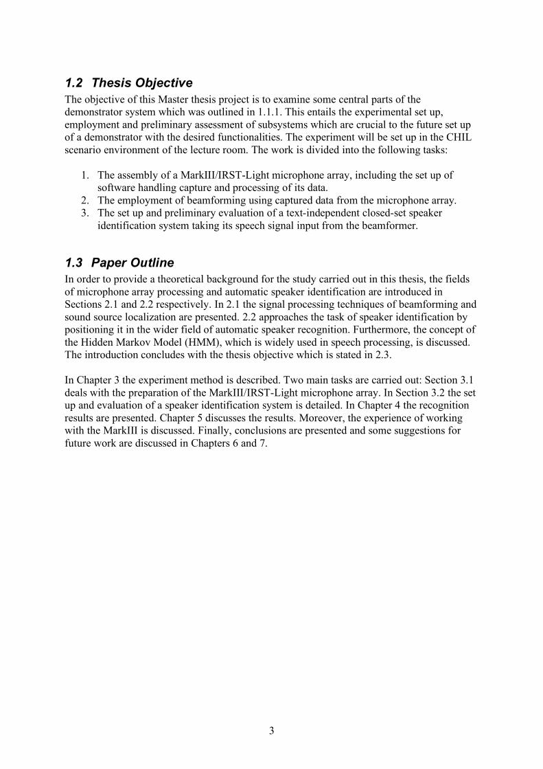
1.2 Thesis Objective The objective of this Master thesis project is to examine some central parts of the demonstrator system which was outlined in 1.1.1. This entails the experimental set up, employment and preliminary assessment of subsystems which are crucial to the future set up of a demonstrator with the desired functionalities. The experiment will be set up in the CHIL scenario environment of the lecture room. The work is divided into the following tasks:

1. The assembly of a MarkIII/IRST-Light microphone array, including the set up of software handling capture and processing of its data.

2. The employment of beamforming using captured data from the microphone array. 3. The set up and preliminary evaluation of a text-independent closed-set speaker

identification system taking its speech signal input from the beamformer.

1.3 Paper Outline In order to provide a theoretical background for the study carried out in this thesis, the fields of microphone array processing and automatic speaker identification are introduced in Sections 2.1 and 2.2 respectively. In 2.1 the signal processing techniques of beamforming and sound source localization are presented. 2.2 approaches the task of speaker identification by positioning it in the wider field of automatic speaker recognition. Furthermore, the concept of the Hidden Markov Model (HMM), which is widely used in speech processing, is discussed. The introduction concludes with the thesis objective which is stated in 2.3. In Chapter 3 the experiment method is described. Two main tasks are carried out: Section 3.1 deals with the preparation of the MarkIII/IRST-Light microphone array. In Section 3.2 the set up and evaluation of a speaker identification system is detailed. In Chapter 4 the recognition results are presented. Chapter 5 discusses the results. Moreover, the experience of working with the MarkIII is discussed. Finally, conclusions are presented and some suggestions for future work are discussed in Chapters 6 and 7.

4

5

Chapter 2: Theory

2.1 Microphone Arrays When recording sound it is important to keep interfering sound sources and noise at a low level compared to the desired signal. The standard way to ensure high SNR for the recorded signal is to place the recording microphone close to the sound source. This will allow the microphone to pick up more of the direct sound in relation to disturbing environmental noise, reverberation and competing sound sources. In some situations, though, like the setting of a lecture room with questions coming from the auditorium, a high number of close-talk microphones would have to be used to ensure that every participating speaker may be recorded in a sufficient way in terms of sound quality. Furthermore, in situations where the ambition is to use technology in an unobtrusive manner, the use of close-talk microphones constitutes an unwelcome element of technology which may divert the attention of the participants. Therefore it is desirable to only use one distant microphone to record all speakers. However, with conventional technology this would render the recorded speech signal more or less unusable due to a poor SNR. One way to solve this issue is by use of a microphone array. Microphone arrays can be designed in a variety of ways but with the shared feature that knowledge of the spatial arrangement of a set of microphone sensors is used to perform signal processing. By processing the data produced by a microphone array, recordings with high SNR can be obtained despite a distance of several meters between the microphone array and the sound source [3]. This is usually realized by use of a technique known as beamforming. Another useful feature of microphone arrays is that they make it possible to compute the direction of arrival (DOA) of an incident sound signal which can be used to work out the position of the sound source. This process is often referred to as sound source localization or speaker tracking. Beamforming and localization will be overviewed in the following sections.

2.1.1 Beamforming A compelling characteristic of microphone arrays is that they make it possible to extract a desired audio signal of high quality from the observations made by its microphone sensors even though, individually, these may be corrupted by noise, reverberation and perhaps other competing sound sources. This extraction can be achieved by applying a beamforming algorithm to the signals picked up by the sensors, enabling a beam to be pointed in a desired direction (sometimes referred to as the look direction). Beamforming reinforces signals from the look direction and attenuates signals from all other directions. Figure 1 shows the structure of the most basic beamformer, namely the delay-and-sum beamformer. A microphone array with N sensors will produce N microphone outputs denoted xn (k) (n = 1,2,…,N). The delay-and-sum beamformer simply delays (or advances) each microphone output so that the signal components from the desired source are synchronized across all sensors. These signals are then weighted and summed together reinforcing signals coming from the look-direction to produce the beamformer output y (k). Sound sources and noise emanating from directions outside the beam are suppressed or even eliminated as they are added together destructively. The weighting coefficients gn can be either fixed or adaptively determined. The latter leads to adaptive beamforming, which allows for cancellation of sounds emanating from directions of choice, by adjusting the weighting coefficients [4].

6

Figure 1: Structure of a delay-and-sum beamformer.

The delay-and-sum technique, however, works best with narrowband signals, and although it is the basis for any array beamforming, more complex algorithms are required to handle broadband signals such as speech. This is because the directivity pattern of a delay-and-sum beamformer changes across a broad frequency band. If a simple delay-and-sum beamformer were to be applied to speech signals we would get a disturbing sound artifact in the array output due to the fact that noise and other disturbing signals would not be uniformly attenuated over its entire spectrum. Several approaches to solve this problem have been suggested and evaluated. One approach is the use of a subband beamforming structure where each of the received signals is decomposed into a set of narrow-band signals. This allows for the time-domain filtering to be performed for each frequency band separately. The output of the subband beamformers are then used to reconstruct a full-band signal [3].

2.1.2 Sound Source Localization Sound source localization has many practical applications such as automatically steering cameras to the current speaker during the course of a video conference or to set the look-direction of a beamformer based on the position of the current speaker. Localization by use of a microphone array involves finding out the direction of arrival (DOA) of an incident waveform. There are many ways to perform DOA estimation using a microphone array. A shared feature among these algorithms, though, is the use of phase information present in the signals picked up by spatially separated sensors [5]. With spatially separated sensors the sound signal will arrive at the sensors with time differences. For an array geometry which is known and with simultaneous recording, these time-delays will be dependent on the DOA of the signal.

y (k)

gN

g2

g1

xN (k)

x2 (k)

x1 (k)

.

.

.

z –T1

z –T2

z –TN

∑

7

2.2 Automatic Speaker Identification This section of the report will introduce the reader to the basic theoretical framework for automatic speaker identification. Firstly, the task of speaker recognition (of which speaker identification is one field of study) will be overviewed. Secondly, the concept of the Hidden Markov Model (HMM) will be presented. Different types of HMMs constitute the core of a variety of speech processing systems.

2.2.1 Speaker Recognition There are several possible strategies to distinguish different voices from each other. Human listeners may derive information about identity from dialect, style of speech and other such high-level information [6]. However, these complex parameters are difficult to implement in automatic systems. Hence, automatic speaker recognition systems tend to focus on acoustical features such as spectral amplitudes, voice pitch frequency and formant frequencies as they are more amenable to automatic processing. Furthermore the speech spectrum has been shown to be very effective for speaker identification [7]. This is because it reflects a person’s vocal tract structure which is an important physical factor influencing the production of the speech signal. Speaker recognition is divided into two main types, namely speaker identification and speaker verification. The distinction between the two is that when performing identification the task is to find the correct speaker among a set of N reference speakers (N possible outcomes), whereas the verification task is to decide whether or not a voice belongs to a specific reference speaker (two possible outcomes) [6]. The performance of speaker identification systems becomes poorer as the number of reference speakers grows. For speaker verification, though, the number of reference speakers will have no influence on the rate with which the system is able to identify the correct speaker. This is one property of verification systems which contributes to generally better conditions for high system performance than for identification systems. Other such factors are that greater control over the speech input often can be maintained, and that the unknown speaker wishes to be recognized and is therefore cooperative. One difficulty not present for speaker identification, but which has do be dealt with in speaker verification, is how to make the decision to accept or reject a speaker3. This entails designing some decision criterion to be able to judge whether an unknown voice sample is similar enough to the voice of the reference speaker, as to be accepted as belonging to the claimed speaker. Speaker identification can be divided into two subcategories: Closed-set identification and open-set identification. Speaker identification as defined above falls under the first category. With open-set identification one more possible outcome is added, namely the possibility that the unknown voice belongs to none of the reference speakers (N+1 outcomes). Open-set identification therefore becomes the most difficult task in speaker recognition, combining the difficulties of closed-set speaker identification and speaker verification [6]. Another property which characterizes a speaker recognition system is whether the system is text-dependent or not. For the case of text-dependent systems, a greater control over the speaker input can be maintained. It is often possible to control the recording environment and also the input speech can be tested against reference speech with the same verbal content.

3 This process is discussed in [8].

8

Text-dependent systems are preferably used with cooperative speakers as is the case with speaker verification systems in which the speaker states his or her identity and possibly some other fixed information [9]. A speaker recognition system which deals with uncooperative speakers is required to be text-independent since there is no way to control what the speaker will actually say. Text-independent systems are also used when recognition must be performed unobtrusively. The greater level of control over text-dependent systems makes them perform better than text-independent systems in general [6].

2.2.1.1 Speech Signal Representation in Recognition Systems The amount of data required to represent the speech waveform is large compared to the rate by which the essential characteristics of the speech process change. Hence the speech characteristics can be represented by less data. Feature extraction techniques for the purpose of speaker recognition aim to extract information which can be used for discrimination, and also to capture this information in a form and size that facilitates further processing4. Speech signals can be parameterized over relatively long time periods of 10 to 25 ms called frames. This enables the amount of data needed for representation of the speech signal to be significantly reduced [10]. Within a frame the speech signal can be approximately regarded as being stationary and may be represented by so called feature vectors or features. Of various feature extraction approaches possible, one of the most commonly used produces so called Mel Frequency Cepstral Coefficients (MFCC). MFCCs may be extracted using band pass filters equally spaced on a mel scale5 from which cepstrum vectors are computed from filter log amplitudes through a cosine transform. The filter bank is usually implemented through weighted sums of FFT points [9]. The number of coefficients is normally 8 to 16 and it is common to also use their first and second time derivatives to make up the feature vectors yielding vectors of 24 to 48 coefficients. The recorded speech signal is not only a consequence of its production, but is also influenced by the environment in a complex way. Factors such as background noise, microphone characteristics and electrical transmission will influence the signal along its transmission path. This calls for robust features which are not unduly affected by such elements. Control over the recording environment enabling low noise and interference levels will improve the performance of speaker recognition. Note that high SNR may also be achieved by use of a microphone array and a beamforming algorithm. Another factor which makes the task of speaker recognition a demanding one is that a single speaker will sound differently from time to time. This phenomenon is called intra-speaker variability. Factors affecting the voice of a speaker may be speech effort level, emotional state, health (e.g. head colds) etc [6]. Speech features need to be robust against this variability as well. It has been shown that the intra-speaker variation grows for data collected over increasing intervals of time. For time intervals exceeding three months, however, the intra-speaker variation will be nearly constant [9]. This may suggest that data collection performed on different occasions over a period of time, will enable a more robust recognition performance.

4 In fact, the same information is often used for speech recognition as for speaker recognition. 5 The use of the mel scale places less emphasis on the high frequencies and is motivated by the fact that it can be used to approximate the frequency resolution in the cochlea.

9

2.2.2 The Hidden Markov Model Hidden Markov Models (HMM) constitute a powerful statistical tool which can be used in various applications. As of today HMMs are being widely used in speech processing technologies, due to their capability of modeling speech signals. An HMM is a stochastic model consisting of a number of states which produce different outputs according to probability density functions associated with the states6. In speech processing applications, Gaussian Mixture Models (GMM) are commonly used to describe the pdf, and the output may be some kind of features representing the characteristics of the speech signal, as described above. The states of an HMM are interconnected by transition probabilities which define the probability to move from one state to another in the model. Probabilities to move back to the same state are also defined (see Figure 2). At regularly spaced discrete times the system undergoes a change of state. The term “hidden” refers to the fact that the HMM process cannot be observed directly. This inherent feature of HMMs will be addressed below. In the experiment reported on in this paper, HMMs will be applied in a text-independent speaker identification system. In this system a special case of the HMM will be used, namely the GMM. The following sections will deal with some basic properties of HMMs which make them suitable for use in speech processing applications. Initially the concept of the Markov chain will be presented. This is followed by the introduction of the fully extended HMM of which the Markov chain forms the basis. The interested reader may learn more about HMMs in [12].

Figure 2: A Markov chain with three states, labelled S1 to S3. State transitions are labelled aij and

represent the probability to move from state i to state j.

6 Alternatively, discrete probabilities may be used but this is uncommon in speech processing [11].

a22

a33

a11

a12

a13

a31 a23

a32

a21

S3

S2 S1

10

2.2.2.1 The Markov Chain A frequently used example for giving an understanding of how Markov models work uses a 3-state Markov chain to model the weather (see Figure 2). Here the outputs of the states are explicitly set to be the following:

State 1: rain State 2: cloudy State 3: sunny

The transition probabilities are set in the matrix A:

This crude model is set to undergo a change of state at a certain time once a day, allowing weather changes to be modeled with the same frequency. In order to account for the possibility that the weather may be unchanged from one day to another, the system has defined probabilities to remain in the same state (or put another way, change back to the same state). Given that the weather on the first day is known and with values assigned to the transition probabilities, the model makes it possible to calculate the probability for a certain weather forecast. If the weather on day one is sunny, the probability that the weather for the next six days will be “sunny, sunny, rain, cloudy, cloudy, sunny” is

a33 · a33 · a31 · a12 · a22 · a23 = = 0.8 · 0.8 · 0.1 · 0.3 · 0.7 · 0.1 = = 1.344 · 10-3

2.2.2.2 Extension to HMM The example above explains how a basic Markov chain may work. However, to be applicable in speech processing the models must have a greater complexity. In a fully developed HMM the states will not correspond directly to one fixed outcome as above. Instead the output from each state is determined by a stochastic process. As a consequence of this the state sequence is not directly observable, since a certain output may have been produced by more than one state. This inability to observe the process has given rise to the term Hidden Markov Model. An HMM is characterized by the number of states in the model, the number of possible outputs (observation symbols) per state, the state transition probabilities, the observation symbol probability distribution in each state and the initial state distribution which gives the probability for the process to have its starting point in each of the different states. HMMs have been described with the term “doubly stochastic process” which refers to the way state transitions are made and how the output from each state is decided in the model [12].

0.4 0.3 0.3 A = {aij} = 0.2 0.7 0.1

0.1 0.1 0.8

11

There are three fundamental problems7 associated with HMMs. Problem 1 can be referred to as the evaluation problem; how do we, given a model and a certain sequence of observations, calculate the probability that the observation sequence was produced by the model. This was solved in a straightforward way for the simple Markov chain model of the weather in the example above. However, for HMMs which feature greater complexity, and as the number of observations grow, direct calculation becomes practically unfeasible due to the vast number of possible state sequences. A more efficient way to solve the evaluation problem is by using the Forward Procedure. Problem 2 is one of trying to find the correct state sequence for a certain set of observations. As was established above, the actual sequence of states is in general not uniquely determinable for an HMM based on the observations8. However, by choosing some optimality criterion it is possible to retrieve some information about the structure of the model and to find optimal state sequences, though this information will be biased by the choice of optimality criterion. One procedure commonly used to approach Problem 2 is the Viterbi Algorithm. Problem 3 is how to modify an HMM to better model real phenomena. This involves optimizing the model parameters in a way that will maximize the probability of a given observation sequence being produced by the model. This complex task is often referred to as training the model. Training requires observation sequences which have some significant properties which the HMM should be able to account for. (An HMM which is supposed to model the word “hello” can be trained using recordings of the word “hello” being spoken.) The observation sequences used to train an HMM can be referred to as training data. There is no known way to analytically solve the training problem, however methods to perform reestimation (iterative update and improvement) of HMM parameters have been developed. One of these is the Baum-Welch method which is widely used in speech processing. The solutions to these three problems are discussed in [12] and can be used to train, adjust and evaluate HMMs. Setting up a speech recognition system may involve creating a number of HMMs, each modelling a speech unit9. Upon recognition the model with the highest evaluated probability to produce the observation at hand may be chosen to represent the speech unit. Thus recognition is completed. Similarly, HMMs trained to model the voice characteristics of speakers can be applied in speaker recognition systems.

2.2.2.3 Parameter Tying A significant problem in constructing HMM systems is that training data is always limited. Data insufficiency will result in parameters being inadequately trained which will lead to poorer recognition performance. Usually a balance must be struck between model complexity and the available data [11]. To make more efficient use of the training data, so called parameter tying may be applied. Parameters such as variances or means may be shared, but higher level tying such as state tying is also possible, resulting in the tied states sharing the

7 The concept of three fundamental problems associated with HMMs was introduced by Jack Ferguson of IDA (Institute for Defence Analysis) and is covered more thoroughly in [12]. 8 This was not the case for the example dealing with the weather, since a Markov chain with fixed and unique state outputs was considered. However such a non-hidden model is too limited in complexity to be applicable in speech processing. 9 A speech unit may be a complete word or a subword such as a phone or a triphone.

12

same pdf. The training data of tied parameters is pooled together, making more training data accessible for the estimation of each individual parameter. Thus tying allows shared parameters to be robustly estimated despite training data being scarce. An example of where tying may be applied is for HMMs modeling the words “to”, “too” and “two”, which are pronounced similarly. These three models may therefore be trained using pooled data from all observations made of these three words.

2.2.2.4 Efficient Modeling for Text-Independent Speaker Identification Returning again to the HMM of Figure 2, it can be noted that from each state of the model, every other state is reachable via some transition. This special type of model can be referred to as an ergodic model. Other layouts of HMMs are also possible and for speech processing the left-right HMM (Figure 3) has been shown to be efficient, since its progression corresponds well to signals whose properties change over time [12].

Figure 3: An example of a left-right HMM. The process starts in S1.

However, for text-independent speaker identification one wants to recognize the overall characteristics of a voice rather than what is being said. This implies that the temporal aspect of the speech signal becomes less significant and the number of states of the HMM can be reduced to one. A 1-state HMM is in effect a GMM (provided that the pdf is defined as a GMM). GMMs have been shown to be an efficient model for text-independent speaker identification systems [13] and in [14] Reynolds et al. argue that the greater complexity of multi-state HMMs seems to provide no advantage over GMM systems when it comes to text-independent recognition.

2.2.2.5 Adaptation To construct a reliable speaker model based on the training data from a single speaker, large amounts of speech from this speaker need to be recorded. Setting up a well-trained model may require hours of training data [11]. Obviously such an approach would be impractical (and increasingly so as the number of enrolled speakers grows). Fortunately techniques exist to adapt an existing model to the voice characteristics of specific speakers using much less speech data. Such techniques are called adaptation techniques and the training data used to customize an existing model may in this case be referred to as adaptation data. The adaptation process reduces the mismatch between an initial model set and the adaptation data by changing the means and possibly also altering the variance parameters of the initial Gaussian mixture system. The parameters are adapted to make the models more likely to generate the adaptation data. A common adaptation task may be to adapt a speech recognition system to a specific speaker in order to enhance the performance of the system for that speaker. On a

a13

a22 a33 a11

a12 a23 S3 S2 S1

13

typical word recognition task, a speaker dependent system may have half the errors of a speaker independent system [11]. For the case of speaker identification, the models of the different speakers may be derived from one universal background model (UBM) which may be a well-trained speaker-independent GMM. The data used to train the UBM should be well balanced so that the model will represent a speaker-independent distribution of features. Thus the model will be trained to represent an average speaker. By adapting the UBM it can be modified to match the voice characteristics of a specific target speaker by use of recorded speech data (adaptation data) from this speaker. The adaptation process is performed once per target speaker to be enrolled in the system and results in one new speaker dependent model per speaker. These models can now be used for identification of the speakers. The process of setting up and adapting a UBM for the purpose of speaker verification is described in more detail in [13]. Several algorithms for performing adaptation have been developed such as the maximum likelihood linear regression (MLLR) technique and the maximum a-posteriori (MAP) approach. Different techniques are used for supervised adaptation, where the true transcription of the adaptation data is known and unsupervised adaptation, which is used for unlabelled data. In the experiment which is reported on below, MAP adaptation is used. The MAP algorithm is a technique for supervised adaptation which aims to maximize the a-posteriori probability of model parameters by relying on a prior knowledge of approximately what they may be [11]. The strength of the MAP technique is that it can rely on the a priori information where there are few adaptation data examples. The prior knowledge is often given by a speaker independent background model, as described above. The influence of the background model compared to the adaptation data can be controlled through weighting.

14

15

Chapter 3: Experiment Method

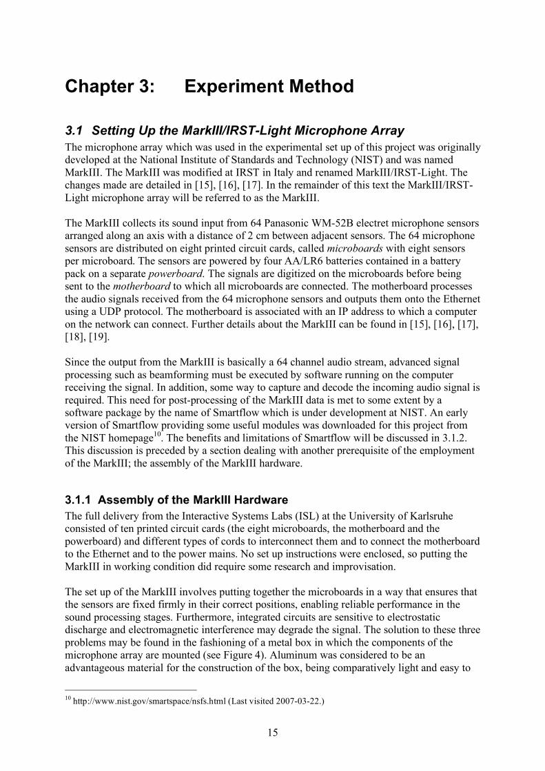
3.1 Setting Up the MarkIII/IRST-Light Microphone Array The microphone array which was used in the experimental set up of this project was originally developed at the National Institute of Standards and Technology (NIST) and was named MarkIII. The MarkIII was modified at IRST in Italy and renamed MarkIII/IRST-Light. The changes made are detailed in [15], [16], [17]. In the remainder of this text the MarkIII/IRST-Light microphone array will be referred to as the MarkIII. The MarkIII collects its sound input from 64 Panasonic WM-52B electret microphone sensors arranged along an axis with a distance of 2 cm between adjacent sensors. The 64 microphone sensors are distributed on eight printed circuit cards, called microboards with eight sensors per microboard. The sensors are powered by four AA/LR6 batteries contained in a battery pack on a separate powerboard. The signals are digitized on the microboards before being sent to the motherboard to which all microboards are connected. The motherboard processes the audio signals received from the 64 microphone sensors and outputs them onto the Ethernet using a UDP protocol. The motherboard is associated with an IP address to which a computer on the network can connect. Further details about the MarkIII can be found in [15], [16], [17], [18], [19]. Since the output from the MarkIII is basically a 64 channel audio stream, advanced signal processing such as beamforming must be executed by software running on the computer receiving the signal. In addition, some way to capture and decode the incoming audio signal is required. This need for post-processing of the MarkIII data is met to some extent by a software package by the name of Smartflow which is under development at NIST. An early version of Smartflow providing some useful modules was downloaded for this project from the NIST homepage10. The benefits and limitations of Smartflow will be discussed in 3.1.2. This discussion is preceded by a section dealing with another prerequisite of the employment of the MarkIII; the assembly of the MarkIII hardware.

3.1.1 Assembly of the MarkIII Hardware The full delivery from the Interactive Systems Labs (ISL) at the University of Karlsruhe consisted of ten printed circuit cards (the eight microboards, the motherboard and the powerboard) and different types of cords to interconnect them and to connect the motherboard to the Ethernet and to the power mains. No set up instructions were enclosed, so putting the MarkIII in working condition did require some research and improvisation. The set up of the MarkIII involves putting together the microboards in a way that ensures that the sensors are fixed firmly in their correct positions, enabling reliable performance in the sound processing stages. Furthermore, integrated circuits are sensitive to electrostatic discharge and electromagnetic interference may degrade the signal. The solution to these three problems may be found in the fashioning of a metal box in which the components of the microphone array are mounted (see Figure 4). Aluminum was considered to be an advantageous material for the construction of the box, being comparatively light and easy to

10 http://www.nist.gov/smartspace/nsfs.html (Last visited 2007-03-22.)

16

work with. Therefore the box was put together mainly using sheet and profile aluminum. In the front side of the box 64 holes were made in which the microphone sensors were fitted. See Appendix B for pictures of the MarkIII.

Figure 4: The interior of the metal box built to enclose the MarkIII hardware. The microboards are mounted on a shelf on the inside of the front side of the box. Each microboard is connected to the motherboard which can be seen below the microboards. The black cables connect the microboards to the powerboard which is not featured in this picture.

3.1.2 Smartflow Smartflow has been developed by NIST as a means to facilitate data transport in the NIST Smart Space11 and Meeting Room Recognition12 projects and has been used to some extent within the CHIL-project. Smartflow can be downloaded from the Smart Space webpage and is delivered with a number of modules performing various tasks such as capturing data from the MarkIII, and different kinds of data conversion13. In addition to this, several signal processing modules such as beamforming and localization clients are included in the package. Smartflow uses a client-server approach where the server acts as a control center to which clients (task performing modules) are connected. The clients communicate via the server by sending information on so-called flows. Using the Smartflow package, however, will reveal that Smartflow is a work in progress. Many of the included clients are not fully developed and some are part of experiment set-ups

11 See http://www.nist.gov/smartspace/ (Last visited 2007-03-22.) 12 See http://www.nist.gov/speech/test_beds/mr_proj/ (Last visited 2007-03-22.) 13 As of 02-08-2007 Smartflow 2 is availible at http://www.nist.gov/smartspace/nsfs.html. In the experiments of this thesis project, Smartflow version 1 was used.

17

which have been abandoned. The disorder is increased by the fact that the Smartflow package is poorly documented. There are few or in many cases no indications as to which clients are in working condition or what tasks they are supposed to perform. However, some information regarding Smartflow can be found in [20], [21]. Another big problem related to the experimental stage of the Smartflow software, is that compilation and installation in the Linux Red Hat environment14 used at TMH is very complicated. Unfortunately the modules for beamforming and localization, of which there are several included, are examples of clients which are either not up-to-date or not functioning at all. However, there are some clients that do work. Examples of operational clients are the mk3cap which performs audio capture of data sent from the MarkIII, and a channel-splitting module used for extracting a mono signal from a selected microphone in the 64 channel mix. These two crucial clients can perform their tasks as stand-alone modules without the employment of the Smartflow control center.

3.1.3 Attempts to Set Up Beamforming Setting up beamforming proved to be a difficult task. The first approach attempted was to use one of the beamforming clients included in the Smartflow package. Great effort was put into the set up of Smartflow, only to find out that none of the several beamforming clients included were operational. The lack of documentation regarding Smartflow in general and the included clients in particular, rendered the challenge of getting a beamforming client up and running a problematical and time-consuming one. In this stage of the process the people at ISL were frequently consulted, sharing their experience of working with the MarkIII and also of examining techniques for beamforming and other advanced processing. However, as no solution could be found, the ambition of performing beamforming within the Smartflow framework was abandoned. During the contacts with ISL in Karlsruhe another possible solution emerged. A module performing delay-and-sum beamforming in the subband domain had been developed for use in experiments at ISL. This beamforming module which was written in Python required the installation of a sound front end processing module and a beamforming toolkit also developed at ISL. These packages and the beamformer were made available via the CHIL framework. However the immaturity of beamforming technology was once more evidenced by the fact that this system also suffered from compatibility problems. This made installation difficult under the Linux Red Hat environment used at TMH. Having had no success with the above attempts to set up of beamforming, the option of developing beamforming software from scratch still remained. However, taking into account that the area of beamforming is just one field of examination included in this project, this added work-load was considered to be too substantial to be included within the scope of a Master thesis. Therefore the goal of performing speaker identification using beamformed speech data had to be abandoned. Instead the speaker identification system was set up and tested using audio data recorded by just one of the microphone sensors of the array. Recordings made by a headset microphone and an omni-directional microphone were also used in the set up of the identification system, which is detailed in the following sections.

14 Linux Red Hat Kernel 2.6.9

18

3.2 Implementation of the Speaker Identification System This section will describe the set up of a ten speaker closed set text-independent speaker identification system. Speaker recognition systems can be designed in a variety of ways, some of which are discussed in [8]. For the purpose of text-independent speaker identification it has been shown that single GMMs are effective for modelling speaker identity15. Therefore the choice was made to set up a system with ten GMMs, each representing a speaker. Furthermore the approach of creating a UBM from which the ten speaker models are derived by MAP adaptation was selected. The benefits of this method are argued in [14], one of the prime motivations being that the amount of adaptation data needed is small. The UBM on the other hand needs to be thoroughly trained, something which requires access to sound recordings of many speakers. A vast amount of speech data collected from Swedish speakers is accessible in the SpeeCon database which was recorded within the SpeeCon project (Speech-Driven Interfaces for Consumer Devices)16. Thus the parameters of the UBM can be estimated using SpeeCon data, bringing the need for new speech data collection to a minimum. Collection of additional speech data is required for the adaptation process where speech data from the ten speakers to be enrolled in the system is an obvious necessity. Also data for testing should be recorded. The speaker identification system was constructed using HTK, which is a toolkit for building HMMs [11]. HTK can be used to set up HMM model sets and also implements solutions to the three problems related to HMMs as discussed in 2.2.2.2. That is to say it provides functionality for evaluating probabilities, finding optimal state sequences and training HMMs. HTK can be used for feature extraction as defined in 2.2.1.1 and also implements algorithms for adaptation and a vast number of other functionalities. HTK is made up of various tools which can be seen as modules performing subtasks in the process of creating and running an HMM system. Some central tools are HCopy which performs front-end processing such as feature extraction, HRest and HERest implementing Baum-Welch reestimation of model parameters, HVite which can work as a Viterbi recognizer and HEAdapt which is used for adaptation. The procedure of initiating and training HMMs in HTK may involve the employment of several HTK tools as well as the execution of numerous other commands. These are preferably put together in a script, something which enables the process to be initiated by a single command and the mode of procedure to be documented. For the speaker identification system set up in this project one script was used for model initiation and training and another for MAP adaptation. The basis for the fashioning of these scripts were scripts used in a Master thesis project carried out at TMH by Lena Måhl [22] who in turn based her work on scripts used in [23]. The remainder of this chapter will focus on the details of the construction of the speaker identification system. Firstly, the set up and training of the UMB is discussed. This is followed by the description of the process of recording adaptation data and test data. Next, the adaptation process using the recorded data is detailed. Finally, assessment of the identification system is discussed.

15 This was discussed in 2.2.2.4. 16 The SpeeCon database is discussed in 3.2.1.1.

19

3.2.1 Creating the Universal Background Model (UBM) This section will go through the process of setting up a single GMM to be used as a speaker-independent background model. For reasons described below, an alternate model design was also tried out and evaluated. This model was set up as a 50-state HMM with all states tied to share the same output distribution, defined by a GMM, providing it with similar characteristics to the single GMM in most respects. The set up processes for the two models are identical for most parts, and the modifications made to acquire the alternate model will be better understood after the original process has been described.

3.2.1.1 Training Data Acquisition The speech data used for training the UBM model was taken from the SpeeCon database, recorded within the SpeeCon project (Speech-Driven Interfaces for Consumer Devices). SpeeCon contains recordings of 550 adult Swedish speakers. The SpeeCon recordings were made in different environments such as in a car, a public place or in an office. The corpus includes recordings of read speech as well as more spontaneous speech. In order to approach free spontaneous speech the subject were given prompts such as “Tell me about your favourite movie” or “Describe the current or a recent traffic situation”17. The speech was recorded on 4 different channels simultaneously, by microphones in different positions. Each of the four speech channels was recorded at 16 kHz with 16-bit quantization. Furthermore an 80 Hz high-pass filter was used. Further information about the SpeeCon database can be found in [24]. Since this experiment is carried out within the CHIL framework, the speaker identification system should be set up to work in a CHIL scenario environment. This was considered in the selection of training data for the UBM. Consequently, only SpeeCon data recorded in the office environment was extracted. For the same reason, the UBM training data was restricted to recordings of spontaneous speech. Another incentive for using data recorded in the office environment is that this category of data in SpeeCon is well balanced with respect to gender (105 females and 101 males) as well as speaker accents. A total of 2055 sound files were extracted from the SpeeCon database, the total length of the recordings amounting to 6 hours and 47 minutes. All recordings had been made using a Sennheiser ME64 Cardioid Condenser Microphone at a distance of 0.5 to 1 m from the speaker.

3.2.1.2 Training Data Parameterization The speech data was parameterized using the HTK tool HCopy to perform MFCC feature extraction. 13 mel frequency cepstral coefficients were computed from a 26-channel, 7.6 kHz bandwidth, mel-scale filter bank. The first coefficient (C0) corresponds to the spectral energy level. The first and second time derivatives were appended to the feature vector bringing the total vector dimension to 39. The frame duration was set to 10 ms.

17 Swedish versions of these prompts were read out loud by the recording assistant whose voice was later edited out of the recordings.

20

3.2.1.3 Training the Background Model The UBM was initiated and trained using HTK tools. The basis for this process was a script used in [22] for training a word recognition system. In that work, HMMs were trained using recordings of utterances of the digits zero to nine, resulting in ten HMMs each modeling one digit. Additionally a silence model was created. This design was modified to set up a UBM represented by a single GMM which was trained on the SpeeCon data. The process of model training involved a data preparation stage where the training data was labeled. For the purpose of training the UBM, a simple dictionary was used, containing the labels “speaker” and “silence”. Labeling of the speech data was carried out using a general pattern of “silence-speaker-silence”. Using this pattern, crude models were trained which were subsequently used in the segmentation process. Segmentation was carried out using so-called forced alignment, which is a process that can be used for automatic data classification. Data labeled as “speaker” was used in the reestimation of the UBM parameters, while data labeled as “silence” was used for the silence model. Thus, two models were initialized; one being a three-state silence model and the other the single GMM used for modeling the characteristics of an average speaker. The GMM was created as a one state HMM18. This was followed by the reestimation of the model parameters using the labeled training data. Next, the models were successively split and reestimated into 2, 4, 8, 16, and 32 Gaussian mixture components. This concluded the training process. Modification of the UBM The rate by which an HMM produces state output is equal to the frame duration used for parameterization of data. For a system using a frame duration of 10 ms and single GMMs to represent speaker identity, identification decisions may consequently occur every 10 ms. It may be desirable that the system should make decisions more seldom, ruling out the unrealistic scenario of a speaker change every 10 ms. This may possibly increase the performance of a multi-speaker19 identification system as it is forced to consider more data before making a decision. For the system reported on here, 0.5 seconds was judged to be a reasonable decision interval. Decreasing the rate by which decisions are made was accomplished through state tying. An alternate UBM was created consisting of a 50-state left-right HMM, with every state sharing the same pdf. No transitions for skipping states were defined, forcing the process to remain in the same model for at least 0.5 s.20 In order to obtain this alternate version of the UBM, state splitting and subsequent tying was implemented using a Gawk script as no HTK functionality could be found for this part of the process. To enable comparison, the system was subsequently evaluated using both UBM versions. A third UBM was also set up using a different parameterization for the training data. The motivation for this can be found in 3.2.3.

18 Actually, in HTK, three states need to be defined since HTK uses non-emitting first and last states as connectors between HMMs. 19 A multi-speaker identification system performs recognition using a grammar which allows for different detection decisions to be made interchangeably. It will become obvious in the latter parts of this report that the system set up in this experiment is a multi-speaker system. 20 If transitions back to the same state occur, 0.5 secons will be exceeded.

21

3.2.2 Data Collection for Adaptation and Testing In order to collect speech data for adaptation and testing, recordings were made of ten Swedish speakers, five men and five women. The setting was the Fantum lecture room at TMH. The dimensions of this room are 11.5 x 7 x 3 meters. The setting of a lecture room was chosen in order to comply with the characteristics of a CHIL scenario. Three recording distances were selected; close, medium and far. Each subject was recorded by the MarkIII at a distance of 4.5 meters from its centre (far). Simultaneously the speech was picked up by a Haun MBNM 550 EL omni-directional microphone at a distance of 1.5 meters (medium) and a Sennheiser ME 104 headset microphone (close). Even though a working beamforming algorithm could not be set up in the scope of this project, the recording process was designed to produce data which could be of use for beamforming experiments to come. Thus the MarkIII was used to make 64 channel recordings of the ten speakers to be enrolled in the speaker identification system. Also five recording positions were selected to enable comparison between different look-directions when performing beamforming (see Figure 5).

Figure 5: The recording positions as seen from above. Angles between all recording positions are 30°.

The five recording positions were set as follows: Position 3 was set to face the microphone array straight ahead (at an angle of 0° to the array normal). Each remaining position was set at an angle of 30° compared to its neighbour. In short, the position angles compared to the array normal can be written as:

Position 1: 60° Position 2: 30° Position 3: 0° Position 4: -30° Position 5: -60°

The subjects were facing the center of the MarkIII during recording. At every change of position the omni-directional microphone was moved and placed on the line between the current position and the centre of the microphone array at a distance of 1.5 m from the

5

4

3

2

1

MarkIII

22

speaker. The recording of each speaker was divided into two sessions separated by a short coffee break of five to ten minutes. In the first session, adaptation data was recorded at all five positions from number 1 through 5. The second session produced the recordings of test data with the positions traversed in the reverse order. The sound picked up by the MarkIII was captured to disc using the mk3cap client which is part of the Smartflow package. This produced 24 bit raw audio recordings with a 22050 Hz sample rate. The ‘close’ and ‘medium’ distance recordings were made using audio recording software by the name of ProTools LE with an MBox interface21. These recordings were stored in wave format with 24 bit resolution and 44.1 kHz sample frequency. The ProTools recordings were divided into phrases (a phrase being one fixed sentence or the response to one prompt) at the recording stage resulting in one phrase per sound file. The MarkIII recordings, however, were stopped only when changing recording positions. As was the case with the speech data used for the training of the UBM, it was found desirable to obtain speech data with characteristics approaching those of spontaneous speech. Therefore the subjects were asked to answer questions similar to those used for prompting spontaneous speech in SpeeCon. The subjects were also asked to read some fixed sentences chosen with the intention of acquiring phonetically balanced adaptation data. These were the same fixed sentences which were used in the TMH Waxholm-project [25]. The prompts and fixed sentences used are listed in Appendix A. MarkIII Data Corruption Inspection of the recorded data revealed that parts of the MarkIII recordings had not been captured due to packet loss. This introduced discontinuities to the recordings, causing transient sound artifacts to appear.

3.2.2.1 Manual Processing of the Collected Speech Data Before the recorded speech data could be parameterized and used for adaptation and testing some manual processing was required. In this process care was taken to provide similar conditions during the subsequent processing. Thus, bit depth and sample frequency should be made equal for all speech data. Moreover, some editing was required in order to remove the voice of the coordinator of the recording sessions. For the data recorded in the ‘close’ and ‘medium’ positions, ProTools was used to edit out unwanted sound data22. This enabled the editing to be carried out identically for both channels. Thus, an equal amount of data was produced for both channels. As the output files from ProTools were wave format files with 24 bit resolution and 44.1 kHz samplerate, requantization and downsampling was required in order to match the specification of the SpeeCon data which was used for training the UBM. Firstly, a sound toolkit by the name of Snack was used to convert the data to 32 bit. Secondly, the data was converted to 16 bit/16 kHz using the sound processing software of Sox with the anti-alias filter rolloff value set to 0.99. The amount of adaptation data and test data collected from the ‘close’ and ‘medium’ positions is accounted for in Table 1.

21 For information about ProTools and the MBox interface, see http://www.digidesign.com (Last visited 2007-03-22.) 22 Unwanted sound data may be the voice of the conductor of the experiment and noises from keystrokes.

23

Table 1: The amount of speech data collected from the ‘close’ and ‘medium’ positions. All numbers denote seconds of speech data, per recorded channel. The data recorded by the MarkIII was captured to 64-channel raw sound files with 24 bit resolution and 22050 Hz samplerate. Since beamforming was not possible, the choice was made to use the sound signal originating from the 32nd microphone sensor of the MarkIII, which is one of two sensors closest to the middle of the array. Using a Smartflow client called channelsplitter, it was attempted to extract the channel 32 data from all 64-channel sound files. For reasons unknown, this was not possible for all sound files. However, some MarkIII data was recovered for all speakers (see Table 2). After the channel extraction, yielding a raw mono sound file, the Wavesurfer sound editor was used to convert the data to 32 bit/22050 Hz wave files. Next, unwanted sound data was edited out. However, no effort was made to edit out the transient noises caused by the data discontinuities, as such editing may affect the speech data as well. In order to obtain matching conditions in latter stages of the process, the phrases in the MarkIII data were cut out and saved to wave files individually. Finally, Sox was employed with rolloff 0.99 to convert the data to 16 bit/16 kHz. Speaker 1 Speaker 2 Speaker 3 Speaker 4 Speaker 5 Speaker 6 Speaker 7 Speaker 8 Speaker 9 Speaker 10 Adaptation Data (s) 149 104 130 247 242 42 77 173 280 327

Test Data (s) 63 41 43 63 54 24 86 41 66 36

Table 2: The amount of speech data collected from the 32nd channel of the MarkIII. All numbers denote seconds of speech data. Due to packet loss during capture and the problems with channel extraction, less data than expected was available for adaptation and testing.

3.2.3 Parameterization of the MarkIII data Due to the transients introduced in the MarkIII data, problems may come up in the adaptation process, as the spectra of the sound files are affected. As a means of decreasing this effect, features which are less sensitive to these sudden changes in the waveform may be computed. It can be argued that removing the time derivative coefficients from the feature vector may yield features which are less sensitive in this respect. Therefore two parallel parameterizations were carried out for the MarkIII data. The first one was identical to the approach used for the SpeeCon data, producing 39-dimension MFCC vectors, including the first and second order deltas. The alternate parameterization process was carried out in the same way but discarded the time derivatives, yielding vectors with 13 elements. For the data collected in the ‘close’ and ‘medium’ positions, only the original parameterization was used. Making use of the alternate data parameterization requires the set up of a new UBM trained on data of the same parameterization. Therefore this parameterization was used for extracting new feature data from the SpeeCon training data. Using this new feature data, a new multi-state UBM was set up, bringing the number of UBMs set up in this experiment to three. The

Speaker 1 Speaker 2 Speaker 3 Speaker 4 Speaker 5 Speaker 6 Speaker 7 Speaker 8 Speaker 9 Speaker 10

Adaptation Data (s) 326 297 185 332 203 171 198 278 422 240

Test Data (s) 115 118 64 118 73 61 151 107 111 70

24

multi-state design was selected as preliminary testing suggested that results were better for the multi-state UMB, than for the single GMM.

3.2.4 Adaptation Adaptation of the UBMs was carried out using the MAP approach as implemented in HEAdapt which features the possibility to control the degree of influence of the adaptation data over the resulting model compared to the influence of the background model. This is achieved by use of a weighting coefficient τ [11]. MAP adaptation in HTK results in a new speaker dependent model with every single mean component updated with a MAP estimate. The alterations are based on the prior mean, the weighting and the adaptation data. Using τ = 0 will cause the means of the resulting speaker model to be equal to the means of the adaptation data. As τ grows, the influence of the background model will increase. By default, variances are not updated by the MAP algorithm used in HEAdapt. The approach of leaving variances unupdated is motivated in [9]. The two UBMs trained on feature data with deltas appended, were adapted to the ten speakers using data collected from all three microphone positions. For data recorded with the MarkIII, two different parameterizations were used, and for the features with deltas missing the third UBM was employed. Adaptation was made for models with 16 as well as 32 Gaussians. This yielded 14 sets of speaker models, each set containing models of the ten speakers. As the value of the MAP adaptation weighting coefficient will influence the parameters of the speaker models, numerous versions of each model set were produced in order to optimize the value of τ.

25

3.3 Assessment of the Speaker Identification System

3.3.1 Recognition The HTK tool HVite can be employed to perform recognition by making a probability evaluation of a set of models with respect to test data. This was done for all versions23 of the 14 speaker model sets respectively. A grammar allowing multi-speaker detection was used. Recognition was consistently carried out using test data which was recorded by the same microphone as the data used for adapting the model set at hand. The output from HVite, which is the model sequence with the highest evaluated probability, may be saved to a file. An excerpt from such a file is shown in Figure 6.

Figure 6: An excerpt of the output file generated by HVite. It is organized as follows: The path within quotation marks points to the location of a test phrase. The path contains information about the microphone used for recording, which speaker was recorded and the number of the test phrase. This information is followed by a section containing the identification results. This information is arranged in three columns. The first two give start and end times of the data examined in 100ns units. This is followed by the identification decision.

23 Versions differ in that thay were adapted using differing values of τ.

"*/proTools/omni/speaker03/mfc-filerTest/t04_16bit_16k.rec" 6000000 12100000 speaker3 43100000 51000000 speaker3 . "*/proTools/omni/speaker03/mfc-filerTest/t03_16bit_16k.rec" 29600000 41700000 speaker3 42200000 47400000 speaker3 58200000 64400000 speaker3 79300000 85000000 speaker3 89200000 94700000 speaker3 104100000 111400000 speaker4 121600000 127300000 speaker3 133000000 143700000 speaker3 . "*/proTools/omni/speaker03/mfc-filerTest/t01_16bit_16k.rec" 58900000 67700000 speaker3 . "*/proTools/omni/speaker03/mfc-filerTest/t05_16bit_16k.rec" 200000 5700000 speaker4 .

26

3.3.2 Evaluation To obtain a value for how well the identification system performs, one possibility would be to simply count the number of correct identification decisions and compare them to the number of incorrect ones. This approach, however, does not take into account the fact that the recognition decisions are made for sections of speech of differing duration. However, both approaches were implemented by the fashioning of a script, which on parsing the HVite output file adds up the time of correct and incorrect decisions as well as the number of correct and incorrect decisions. The script calculates recognition performance ratios for each test phrase and also adds up a total score for the entire model set based on the performance on all test phrases.

27

Chapter 4: Results In this chapter the results of this Master thesis project are accounted for. The main focus of the chapter will be the presentation of the identification performance of the speaker identification system. However it should also be noted that an important additional outcome of the effort invested in this project is the preparation of the MarkIII, which may be used for further experiments with microphone array processing. During the construction of the speaker identification system, three different UBMs were trained. The approach of using a single GMM for modelling speaker identity was used for the first background model. The second UBM is a multi-state left-right HMM with all states sharing the same output distribution represented by a GMM. The structures of the second and third UBMs are identical but they differ due to different parameterizations of the data used for training. The third UBM, which was trained using features without deltas appended, was only adapted using data collected with the MarkIII. The characteristics of the three UBMs are listed in Table 3.

Model Structure Parameterization

UBM 1 Single GMM MFCC, deltas included

UBM 2 Multi-tied-state HMM MFCC, deltas included

UBM 3 Multi-tied-state HMM MFCC, no deltas Table 3: Characteristics of the three UBMs.

The MAP adaptation process which followed resulted in 14 main sets24 of ten speaker models, each set in itself sufficient to be used for recognition in HTK. In order to find an optimal value for the weighting coefficient τ for each set, numerous adaptations were made providing different versions of the main model sets. Identification performance was assessed for all model sets. The identification performance for the main sets with optimized τ is illustrated in Figure 7. The results for model sets with the value of τ varied are detailed in the Figures 8-10. Here, the results for some values of τ are omitted due to the large number of adaptations made. Moreover, different model sets were evaluated using different values of τ, which explains the gaps in these diagrams. The performance measure used in all charts is the False Detection Rate stated in percent. The False Detection Rate was calculated by dividing the amount of data where false detection decisions were made by the amount of test data considered. The calculations were based on the time duration of correct and incorrect decisions.

24 Two UMBs were adapted with data recorded from all 3 recording positions to produce 6 speaker sets. The third UBM was adapted only using data from the MarkIII, increasing the number of speaker sets by 1. The training process of all speaker models produced models with 2, 4, 8, 16 and 32 Gaussian mixtures making up the GMMs. Recognition was made using models with 16 and 32 Gaussians bringing the total number of evaluated speaker sets to 14.

28

Optimized _

0

10

20

30

40

50

60

70

80

90

Fals

e D

ete

cti

on

Rate

Multi-state, 16 Gaussians 27,43 19,35 45,92 66,29

Multi-state, 32 Gaussians 25,15 16,96 48,50 61,41

Single-state, 16 Gaussians 46,77 44,64 76,62

Single-state, 32 Gaussians 48,05 42,24 71,15

Close Medium Far1 Far2

Figure 7: Identification results for the 14 main speaker model sets with optimized τ. The results from different recording positions are grouped together. ‘Far1’ denotes model sets which were adapted using data from the MarkIII with the original parameterization (deltas appended). ‘Far2’ denotes model sets which were adapted using data from the MarkIII with the alternate parameterization (deltas discarded). Within groups, four different model designs are featured. These are combinations of single-state or multi-state UBMs with output distributions made up of 16 or 32 Gaussians. As expected, evaluation of the speaker sets which were adapted and tested on speech data picked up by the single MarkIII sensor shows a significantly higher False Detection Rate than other speaker sets of analogous design. The main reason for this may be that the recording distance was greater for the MarkIII microphone sensor than for the headset and omni-directional microphones, resulting in poorer SNR for the MarkIII sensor recordings. It should also be noted that the MarkIII speaker sets were adapted using less adaptation data and that this data was corrupted by packet loss. The attempt to reduce the effect of the discontinuities present in the MarkIII data by using an alternate parameterization did not increase the recognition performance. It can be seen from the Figures 8-10, that the approach of using a multi-tied-state speaker model seems to provide an advantage over the single GMM approach. The differences in performance induced by changing between GMMs made up by 16 and 32 Gaussians were much smaller in comparison. The best performance was achieved by using data collected from the medium distance recording position and applying adaptation with τ = 48 to the multi-tied-state UBM with 32 Gaussian mixtures in the output distribution. This speaker set yielded a False Detection Rate of 17 %. Results for models adapted with big τ are unreliable as this made the recogniser classify less of the test data as speech.

29

Close Recording Position

0

10

20

30

40

50

60

70

_

Fals

e D

ete

cti

on

Rate

(%

)

Single-state, 16 Gaussians 46,8 49,8 50,9 53,6 56,3 62,2 60,6 62

Single-state, 32 Gaussians 48 51,6 53,5 54,9 54,5 54,1 53,9 52,4

Multi-state, 16 Gaussians 27,4 27,4 27,4 27,5 27,6 27,7 27,9 28,1 28,4 28,9 29,3 30,7 32,9 34,6 43,7 49,8 44,2

Multi-state, 32 Gaussians 25,4 25,3 25,1 25,5 25,6 25,5 25,8 26,1 26,1 26,2 26,2 26,9 27,6 27,9 29 31,1 34,8 37,8 47,9 42,4 40,2

0 0,1 0,2 0,3 0,4 0,5 0,6 0,7 0,8 0,9 1 2 3 4 5 10 20 30 100 500 1000

Figure 8: Identification results for speaker model sets adapted using data from the ‘close’ recording position with τ varied.

Medium Recording Position

0

10

20

30

40

50

60

70

_Fals

e D

ete

cti

on

Rate

(%

)

Single-state, 16 Gaussians 52,8 48,7 46,7 44,6 45,2 44,9 46,2 51,1 52,1

Single-state, 32 Gaussians 50,1 44,6 42,2 42,6 43,7 44,9 47,4 53,1 57,5

Multi-state 16 Gaussians 27,2 26,8 25,6 24,3 23,6 22,7 22,6 21,8 20,7 21,6 21,6 21,7 21,5 20,5 19,5 19,5 19,4 19,4 19,7 19,7 20,4 20,5 23,4 27,7

Multi-state, 32 Gaussians 25 23,9 22,4 19,4 18,7 19,1 17,3 17,2 17,4 17,5 17 17,7 17,5 18,6 19,4 21,4 21,9 23,4 26,8 26,6

0 5 10 20 25 30 38 39 40 47 48 49 50 60 70 80 90 100 150 200 238 239 240 241 242 250 260 300 500 1000

Figure 9: Identification results for speaker model sets adapted using data from the ‘medium’ recording position with τ varied.

30

Far Recording Position

0

10

20

30

40

50

60

70

80

90

100

_

Fals

e D

ete

cti

on

Rate

(%

)

Single-state, 16 Gaussians 76,6 77,9 81,8 81,3 83,7 86 90,6 93,9 93,8

Single-state, 32 Gaussians 78,2 76 74,2 71,1 71,2 88,3 59 54,5

Multi-state, 16 Gaussians 46,2 46 45,9 46,7 46,7 46,8 47,3 48,2 49,6 50,5 52,1 54,1 55,5 55,5 58,1 60 61,4 62,7 64,3 71,9 75,5 84,8 89,1

Multistate, 32 Gaussians 48,5 49,2 49,7 49,9 50,2 50,9 51,5 52,4 52,6 57,4 60,4 62,1 71 79,3 75,9

Multi-state, 16 Gaussians, No _ 71,8 72,6 72,3 69,2 68,4 66,3 67,2 85 91,9

Multi-state, 32 Gaussians, No _ 68,8 62,3 61,4 62,6 63,1 65 67,7 87 90,2

0 0,1 0,2 0,3 1 2 3 4 5 10 20 30 40 50 60 70 80 90 100 150 200 500 1000

Figure 10: Identification results for speaker model sets adapted using data from the ‘far’ recording position with τ varied. No Δ denotes that the deltas were not appended to the feature vector during parameterization.

31

Chapter 5: Discussion

5.1 Working with the MarkIII A microphone array may be used as a powerful tool when combined with efficient signal processing such as beamforming and sound source localization. The prospect of combining this processing with speech technology like speech and/or speaker recognition may form the basis for systems of various functionalities. One possibility is the system which was envisioned at the starting point of this thesis project. The experience of working with the state-of-the-art MarkIII/IRST-Light microphone array shows that further development of the technology is needed before any ease-of-use can be obtained. In retrospect it is obvious that the set up of the real-time demonstrator, which was outlined initially, is a task of great complexity. A main problem was the immaturity of the Smartflow software package which has been developed by NIST partly for processing of the array output. In the end only two Smartflow clients were used: mk3cap for data capture and a channel extraction module. These were offline stand-alone clients so the dataflow part of the Smartflow was never used. As of 02-08-2007 a new version of the software, dubbed Smartflow 2, is available for download at the NIST webpage. Possibly this will make for more efficient data processing. The effort made to assemble the MarkIII hardware and to make use of the output data did result in 64 channel recordings. These, however, were corrupted by packet loss making the prospect of using them for future testing of beamformer algorithms an unpromising one. Similar problems were experienced when trying to compile and install the toolkits and modules for beamforming acquired from ISL in Karlsruhe. Despite the helpful assistance of the people of ISL the problem could not be given a final solution. Thus, no operational beamformer could be set up within the scope of this project and other aspects of interest were pursued.

5.2 Reflections Regarding the Identification Results A basic problem when recording audio is that, with conventional technology, the quality of the recorded signal will deteriorate as the recording distance grows. This will have implications for further processing of the recorded data. Therefore one would expect deterioration in speaker detection performance when comparing the results based on the recording positions ‘close’, ‘medium’, and ‘far’ in that order. However, the results indicate that recognition performance was best for speaker model sets adapted using data from the medium-distance position. An explanation for this may be that the transmission path for data recorded using this channel may be more similar to the transmission path of the SpeeCon data recordings. An important aspect may be that the recording distance for the SpeeCon data was approximately in the same range as the medium distance used when recording adaptation and test data. As expected, False Detection Rates were considerably higher for model sets adapted using data recorded from the ‘far’ position. However, the poor recognition performance for these models may partly be due to the problem with MarkIII data corruption and that less adaptation

32

data was available for the model sets using MarkIII data than for other sets. The attempt to reduce the effect of the discontinuities present in the MarkIII data by discarding the time derivative features did not work out as hoped. Instead the False Detection Rate increased from 46 % to 66 % and 49 % to 61 % for 16-Gaussian and 32-Gaussian models respectively. Obviously important information was lost when the deltas were discarded from the feature vectors.

5.2.1 Amount of Adaptation Data Some speaker model sets showed best results when τ was set to 0. This implies that the speaker model means are solely determined by the adaptation data. Thus the adaptation process makes no use of this a priori information of the UBM. As variances were not updated by the adaptation approach used, these were taken from the UBM. A greater amount of adaptation data may have provided better performance from the MAP adaptation. The differences in performance for model sets with 32 Gaussian mixture distributions and sets with 16 Gaussians were small. For the models with 16 Gaussians more data was available for each parameter and therefore they may have been more thoroughly estimated. More adaptation data may have increased the performance of model sets with 32 Gaussians compared to those with 16 Gaussians.

5.2.2 Robustness of the Speaker Identification System Since little time passed between the recording of adaptation data and test data, identification results can be expected to deteriorate for test data collected at later occasions due to intra-speaker variability as discussed in 2.2.1.1. In order to cope with this problem adaptation data would have to be collected at a number of occasions spread out over a period of time. This may increase the robustness of the speaker models.

33

Chapter 6: Conclusions This Master thesis project has focused on two important fields of study in the context of unobtrusive technology; the microphone array and speaker recognition. The work, which has been carried out within the CHIL framework, has included the assembly and employment of a MarkIII/IRST-Light microphone array and the set up and evaluation of a ten speaker text-independent closed-set speaker identification system. Beamforming, which is a technique for audio signal enhancement, was given special attention. The beamforming algorithm makes use of the multi-channel output from the microphone array to achieve noise and interference reduction. However, the ambition to set up an operational beamformer within the scope of this project had to be abandoned for the benefit of other tasks. For the speaker identification system the approach of deriving speaker models from a Universal Background Model by MAP adaptation was adopted. Two similar speaker model designs were employed. The original design used a single GMM for modeling speaker identity. This approach formed the basis for the alternate multi-state model in which all states were tied, thus sharing the same output distribution. Preliminary evaluation showed considerably lower False Detection Rates for models of the multi-state design.

34

35

Chapter 7: Future Work The work carried out within this project may provide the foundation for further TMH-based research into the field of microphone array processing. The set up of an operational beamforming module is essential. Two alternative approaches are suggested: A new attempt to set up and use the subband beamformer acquired from ISL could be launched. This would most likely require the assistance of the people at ISL who possess knowledge of how this Python script based beamformer should be operated. The other alternative would be to develop a beamformer from scratch. This inspiring task would probably make up a Master thesis project in itself. For the combination of beamforming with speaker identification, proper use of a beamforming algorithm should improve the SNR and therefore lower the amount of false identification decisions. Thus, the use of an efficient beamformer in the ‘far’ position may yield recognition performance results approaching those obtained from closer recording distances. However, the discontinuities present in the MarkIII data recorded in this project would probably cause the beamformer to perform poorly. Therefore new 64-channel data may need to be recorded. In order to solve the packet loss problem a separate network card dedicated to receive the MarkIII data should be used. Furthermore, the Linux kernel may need to be tuned. Some instructions for this procedure can be found in [26]. Another improvement, which was suggested by ISL, would be to fit the inside of the aluminum box with foam in order to reduce resonances within the enclosure. If the above tasks are carried out successfully, the realization of the demonstrator which was outlined initially may be possible. The main issue to be dealt with will probably be that real-time processing will be required. Hopefully, Smartflow 2 may solve the real-time data transport up to the point of delivering a beamformed audio signal to the speaker recognition system. HTK includes functionality for recognition using direct audio input [11, p. 41 and 188]. Moreover, the technique of sound source localization need to be further researched. Within the CHIL framework so-called T-shaped arrays have been used to perform 3D localization. To conclude, some additional analysis may be carried out for the experiment carried out in this project. It would be interesting to evaluate the performance for values of τ > 1000. Furthermore, recognition performance on test data recorded by a channel different from the channel used for adaptation data acquisition may be evaluated.

36

37

References

[1] Svanfeldt, Gunilla and Olszewski, Dirk: Perception Experiment Combining a Parametric Loudspeaker and Synthetic Talking Head, Proceedings of Interspeech 2005, pp. 1721-1724

[2] Beskow, J., Karlsson, I., Kewley, J., and Salvi, G.: SYNFACE – A Talking Head

Telephone for the Hearing-impaired, In Miesenberger, K., Klaus, J., Zagler, W., & Burger, D. (Eds.), “Computers Helping People with Special Needs” pp. 1178-1186 Springer-Verlag, 2004

[3] Yermeche, Zohra: Subband Beamforming for Speech Enhancement in Hands-Free

Communication, Licentiate Thesis, Blekinge Institute of Technology, Karlskrona, 2004

[4] Benesty, J., Chen, J., Huang, Y., Dmochowski, J.: On Microphone-Array

Beamforming From a MIMO Acoustic Signal Processing Perspective, IEEE Transactions on Audio, Speech and Language Processing Volume 15, Issue 3, March 2007, pp. 1053 - 1065

[5] Varma, Krishnaraj: Time-Delay-Estimate Based Direction-of-Arrival Estimation for

Speech in Reverberant Environments, Master Thesis, Virginia Polytechnic Institute and State University, Blacksburg, Oct 2002

[6] Doddington, George R.: Speaker Recognition – Identifying People by their Voices,

Proceedings of the IEEE, Vol. 73, No. 11, November 1985, pp. 1651 - 1664

[7] Atal, B.S.: Automatic Recognition of Speakers from Their Voices, Proceedings of the IEEE, Volume 64, Issue 4, April 1976 pp. 460 - 475

[8] Campbell, Joseph P. JR.: Speaker Recognition: A Tutorial, Proceedings of the IEEE,

Vol. 85, No. 9, September 1997, pp. 1437 - 1462

[9] Melin, Håkan: Automatic Speaker Verification on Site and by Telephone: Methods, Applications and Assessment, PhD Thesis, KTH, Stockholm, December 2006

[10] Gish, Herbert and Schmidt, Michael: Text-Independent Speaker Identification, Signal

Processing Magazine, IEEE Volume 11, Issue 4, October 1994 pp. 18 - 32

[11] Young, S., Kershaw D., Odell, J, Ollason, D., Valtchev, V., Woodland, P.: The HTK Book (for HTK Version 3.2), Entropic Cambridge Research Laboratory, December 2002

[12] Rabiner, Lawrence R.: A Tutorial on Hidden Markov Models and Selected

Applications in Speech Recognition, Proceedings of the IEEE, Vol. 77, No. 2, February 1989, pp. 257 - 286

38

[13] Reynolds, Douglas A. and Rose, Richard C.: Robust Text-Independent Speaker Identification Using Gaussian Mixture Speaker Models, IEEE Transactions on Speech and Audio Processing, Vol. 3 No. 1, January 1995, pp. 72 - 83

[14] Reynolds, D. A., Quatieri, T. F. and Dunn R. B.: Speaker Verification Using Adapted

Gaussian Mixture Models, Digital Signal Processing 10, 2000, pp. 19-42

[15] Bertotti, C, Brayda, L., Cristoforetti, L., Omologo, M., Svazier, P.: The MarkIII microphone array: the modified version realized at ITC-irst, URL: http://www.eurecom.fr/~brayda/MarkIII-IRST.pdf (Last visited 2007-03-22.)

[16] Bertotti, C, Brayda, L., Cristoforetti, L., Omologo, M., Svazier, P.: The new

MarkIII/IRST-Light microphone array, URL: http://www.eurecom.fr/~brayda/MarkIII-IRST-Light.pdf (Last visited 2007-03-22.)

[17] Brayda, L., Bertotti, C, Cristoforetti, L., Omologo, M., Svazier, P.: Modifications on

NIST MarkIII array to improve coherence properties among input signals, Journal of Audio Engineering Society, 2005

[18] Rochet, Cedrick: Technical Documentation of the Microphone Array Mark III

National Institute of Standards and Technology, September 2005, URL: http://www.nist.gov/smartspace/toolChest/cmaiiiv2/Technical_Documentation_Mark_III/Technical_Documentation_Mark_III.pdf (Last visited 2007-03-22.)

[19] Rochet, Cedrick: User’s Manual of the Microphone Array Mark III version 2,

National Institute of Standards and Technology, Interactive Systems Labs Universität Karlsruhe, September 2005, URL: http://www.nist.gov/smartspace/toolChest/cmaiiiv2/Microphone_Array_Mark_III_version_2/Microphone_Array_Mark_III_version_2.pdf (Last visited 2007-03-22.)

[20] Martin, C., Galibert, O., Michel, M., Mougin, F., Stanford V.: NIST Smart Data-Flow

System Programmer’s guide Version 3.6, National Institute of Standards and Technology, USA, July 2000 URL: http://www.nist.gov/smartspace/toolChest/nsfs/dataFlow/progG/NSFS_programmerGuide.pdf (Last visited 2007-03-22.)

[21] Martin, C., Galibert, O., Michel, M., Mougin, F., Stanford V.: NIST Smart Data-Flow

System User’s guide Version 3.6, National Institute of Standards and Technology, USA, July 2000, URL: http://www.nist.gov/smartspace/toolChest/nsfs/dataFlow/userG/NSFS_userGuide.pdf (Last visited 2007-03-22.)

[22] Måhl, Lena: Speech recognition and adaptation experiments on children’s speech,

Master Thesis, TMH, KTH, 2004

[23] Lindberg, B., Johansen, F. T., Warakagoda, N., Lehtinen, G., Kai, Z., Gank, A., Elenius, K., and Salvi, G.: A Noise Robust Multilingual Reference Recogniser Based on SpeechDat(II), Proc of ICSLP, 6th Intl Conf on Spoken Language Processing, 2000 pp. 370-373

39

[24] Dorota Iskra, D., Grosskopf, B., Marasek, K., van den Heuvel, H., Diehl, F., Kiessling, A.: SPEECON - Speech Databases for Consumer Devices: Database Specification and Validation, In Manuel Gonzáles Rodríguez & Carrmen Suárez Araujo (Eds.), Proceedings LREC 2002. Third International Conference on Language Resources and Evaluation, Paris: ELRA, European Language Resources Association.

[25] Blomberg, M., Carlson, R., Elenius, K. O. E., Granström, B., Gustafson, J., Hunnicutt,

S., Lindell, R., Neovius, L., and Nord, L.: An Experimental Dialogue System: Waxholm, STL-QPSR 2-3/93. URL: http://www.speech.kth.se/prod/publications/files/1109.pdf (Last visited 2007-03-22.)

[26] URL:

http://www.nist.gov/smartspace/toolChest/cmaiii/userg/Microphone_Array_Mark_III/node29.html (Last visited 2007-03-22.)

40

41

Appendix A: Prompts for Speech Data Acquisition Prompts for Spontaneous Speech

1. Beskriv hur man går härifrån till Sergels torg!

2. Berätta lite om en bra film du sett!

3. Vad planerar du att göra till sommaren?

4. Vad tycker du om att göra på din fritid?

5. Beskriv vad jobbar du med! 6. Beskriv gårdagens middag!

7. Vilken stad skulle du vilja bo i och varför?

8. Räkna upp intressanta platser/attraktioner i den här staden!

9. Vilket land skulle du vilja resa till och varför?

10. Beskriv den aktuella eller en nyligen inträffad trafiksituation!

11. Ge en beskrivning hur man kommer till ett trevligt café i närheten av där du befinner dig eller där du bor!

12. Beskriv ditt favorit-TV-program!

13. Beskriv din favoritsport och din favoritutövare av den!

14. Vad är ditt intryck av inspelningen så här långt?

15. Vilken typ av utrustning skulle du vilja kontrollera med hjälp av din röst?

16. Hur föreställer du dig att det skulle fungera? (Exempel: mixer, diskmaskin, tvättmaskin, dammsugare, dörrlås)

Fixed Sentences 1. Vaxholm ligger i Stockholms skärgård. 2. Lila stolar bärs in i salen. 3. Fortkörning är värre än mord, sa konstapel Thörnhjort. 4. Det var kyligt i luften och stjärnorna skimrade. 5. Lediga och utvilade tittade dom på föreställningen i en timme. 6. Sprakande fyrverkeripjäser exploderade över oss. 7. Där kommer nya röda hus att skjuta i höjden. 8. Öppna dörren innan jag fryser ihjäl.

42

43

Appendix B: Photographs of the MarkIII

Picture 1: The assembled MarkIII/IRST-Light microphone array

Picture 2: The powerboard with the batterypack

as seen from inside the box

Picture 3: The front of the batterypack,

powerswitch and battery indicator

44

Picture 4:Close-up on the microphone sensors

Picture 5: One of the eight microboards

TRITA-CSC-E 2007:076 ISRN-KTH/CSC/E--07/076--SE

ISSN-1653-5715

www.kth.se