Aspen Tasc Thermal Reference Guide

Copyright Version Number: 2004

Copyright 1981 - 2004 Aspen Technology, Inc. All rights reserved.

Aspen ACOL™, Aspen ACX™, Aspen APLE™, Aspen Adsim™, Aspen Aerotran™, Aspen CatRef®, Aspen Chromatography®, Aspen Custom Modeler®, Aspen Decision Analyzer™, Aspen Dynamics®, Aspen Enterprise Engineering™, Aspen FCC®, Aspen Hetran™, Aspen Hydrocracker®, Aspen Hydrotreater™, Aspen Icarus Process Evaluator™, Aspen Icarus Project Manager™, Aspen Kbase™, Aspen Plus®, Aspen Plus® HTRI®, Aspen OLI™, Aspen OnLine®, Aspen PEP Process Library™, Aspen Plus BatchFrac™, Aspen Plus Optimizer™, Aspen Plus RateFrac™, Aspen Plus SPYRO®, Aspen Plus TSWEET®, Aspen Split™, Aspen WebModels™, Aspen Pinch®, Aspen Properties™, Aspen SEM™, Aspen Teams™, Aspen Utilities™, Aspen Water™, Aspen Zyqad™, COMThermo®, COMThermo TRC Database™, Aspen DISTIL™, Aspen DISTIL Complex Columns Module™, Aspen FIHR™, Aspen FLARENET™, Aspen FRAN™, Aspen HX-Net®, Aspen HX-Net Assisted Design Module™, Aspen Hyprotech Server™, Aspen HYSYS®, Aspen HYSYS Optimizer™, ACM Model Export™, Aspen HYSYS Amines™, Aspen HYSYS Crude Module™, Aspen HYSYS Data Rec™, Aspen HYSYS DMC+ Link™, Aspen HYSYS Dynamics™, Aspen HYSYS Electrolytes™, Aspen HYSYS Lumper™, Aspen HYSYS Neural Net™, Aspen HYSYS Olga Transient™, Aspen HYSYS OLGAS 3-Phase™, Aspen HYSYS OLGAS™, Aspen HYSYS PIPESIM Link™, Aspen HYSYS Pipesim Net™, Aspen HYSYS PIPESYS™, Aspen HYSYS RTO™, Aspen HYSYS Sizing™, Aspen HYSYS Synetix Reactor Models™, Aspen HYSYS Tacite™, Aspen HYSYS Upstream™, Aspen HYSYS for Ammonia Plants™, Aspen MUSE™, Aspen PIPE™, Aspen Polymers ®, Aspen Process Manuals™, Aspen BatchSEP™, Aspen Process Tools™, Aspen ProFES 2P Tran™, Aspen ProFES 2P Wax™, Aspen ProFES 3P Tran™, Aspen ProFES Tranflo™, Aspen STX™, Aspen TASC-Thermal™, Aspen TASC-Mechanical™, the aspen leaf logo and Enterprise Optimization are trademarks or registered trademarks of Aspen Technology, Inc., Cambridge, MA.

All other brand and product names are trademarks or registered trademarks of their respective companies.

This document is intended as a guide to using AspenTech's software. This documentation contains AspenTech proprietary and confidential information and may not be disclosed, used, or copied without the prior consent of AspenTech or as set forth in the applicable license agreement. Users are solely responsible for the proper use of the software and the application of the results obtained.

Although AspenTech has tested the software and reviewed the documentation, the sole warranty for the software may be found in the applicable license agreement between AspenTech and the user. ASPENTECH MAKES NO WARRANTY OR REPRESENTATION, EITHER EXPRESSED OR IMPLIED, WITH RESPECT TO THIS DOCUMENTATION, ITS QUALITY, PERFORMANCE, MERCHANTABILITY, OR FITNESS FOR A PARTICULAR PURPOSE.

Introduction

Corporate

Aspen Technology, Inc. Ten Canal Park Cambridge, MA 02141-2201 USA Phone: (1) (617) 949-1000 Toll Free: (1) (888) 996-7001 Fax: (1) (617) 949-1030 URL: http://www.aspentech.com/

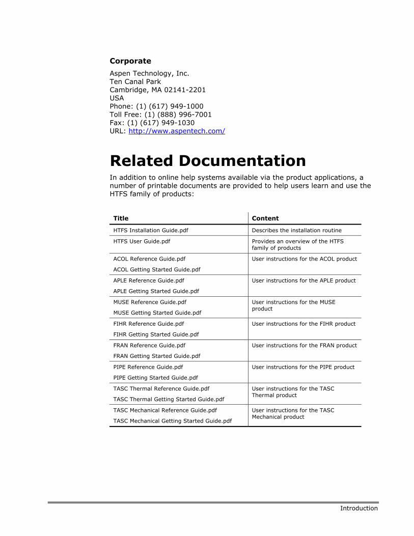
Related Documentation In addition to online help systems available via the product applications, a number of printable documents are provided to help users learn and use the HTFS family of products:

Title Content

HTFS Installation Guide.pdf Describes the installation routine

HTFS User Guide.pdf Provides an overview of the HTFS family of products

ACOL Reference Guide.pdf

ACOL Getting Started Guide.pdf

User instructions for the ACOL product

APLE Reference Guide.pdf

APLE Getting Started Guide.pdf

User instructions for the APLE product

MUSE Reference Guide.pdf

MUSE Getting Started Guide.pdf

User instructions for the MUSE product

FIHR Reference Guide.pdf

FIHR Getting Started Guide.pdf

User instructions for the FIHR product

FRAN Reference Guide.pdf

FRAN Getting Started Guide.pdf

User instructions for the FRAN product

PIPE Reference Guide.pdf

PIPE Getting Started Guide.pdf

User instructions for the PIPE product

TASC Thermal Reference Guide.pdf

TASC Thermal Getting Started Guide.pdf

User instructions for the TASC Thermal product

TASC Mechanical Reference Guide.pdf

TASC Mechanical Getting Started Guide.pdf

User instructions for the TASC Mechanical product

Introduction

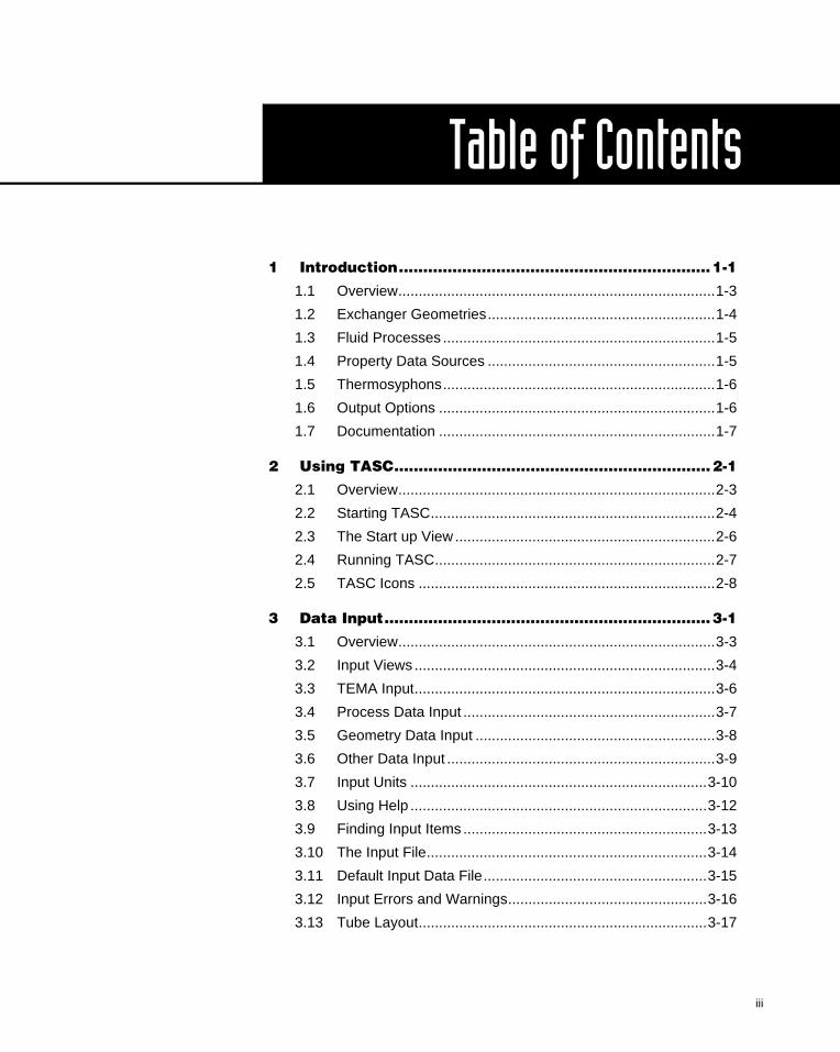
Table of Contents

1 Introduction................................................................1-1

1.1 Overview..............................................................................1-3

1.2 Exchanger Geometries........................................................1-4

1.3 Fluid Processes ...................................................................1-5

1.4 Property Data Sources ........................................................1-5

1.5 Thermosyphons...................................................................1-6

1.6 Output Options ....................................................................1-6

1.7 Documentation ....................................................................1-7

2 Using TASC.................................................................2-1

2.1 Overview..............................................................................2-3

2.2 Starting TASC......................................................................2-4

2.3 The Start up View ................................................................2-6

2.4 Running TASC.....................................................................2-7

2.5 TASC Icons .........................................................................2-8

3 Data Input...................................................................3-1

3.1 Overview..............................................................................3-3

3.2 Input Views ..........................................................................3-4

3.3 TEMA Input..........................................................................3-6

3.4 Process Data Input ..............................................................3-7

3.5 Geometry Data Input ...........................................................3-8

3.6 Other Data Input ..................................................................3-9

3.7 Input Units .........................................................................3-10

3.8 Using Help .........................................................................3-12

3.9 Finding Input Items ............................................................3-13

3.10 The Input File.....................................................................3-14

3.11 Default Input Data File.......................................................3-15

3.12 Input Errors and Warnings.................................................3-16

3.13 Tube Layout.......................................................................3-17

iii

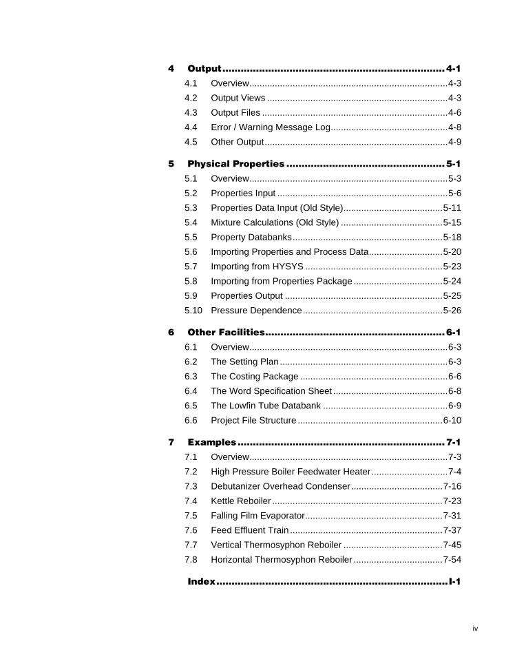
4 Output.........................................................................4-1

4.1 Overview..............................................................................4-3

4.2 Output Views .......................................................................4-3

4.3 Output Files .........................................................................4-6

4.4 Error / Warning Message Log..............................................4-8

4.5 Other Output........................................................................4-9

5 Physical Properties ....................................................5-1

5.1 Overview..............................................................................5-3

5.2 Properties Input ...................................................................5-6

5.3 Properties Data Input (Old Style).......................................5-11

5.4 Mixture Calculations (Old Style) ........................................5-15

5.5 Property Databanks...........................................................5-18

5.6 Importing Properties and Process Data.............................5-20

5.7 Importing from HYSYS ......................................................5-23

5.8 Importing from Properties Package ...................................5-24

5.9 Properties Output ..............................................................5-25

5.10 Pressure Dependence.......................................................5-26

6 Other Facilities...........................................................6-1

6.1 Overview..............................................................................6-3

6.2 The Setting Plan ..................................................................6-3

6.3 The Costing Package ..........................................................6-6

6.4 The Word Specification Sheet .............................................6-8

6.5 The Lowfin Tube Databank .................................................6-9

6.6 Project File Structure .........................................................6-10

7 Examples ....................................................................7-1

7.1 Overview..............................................................................7-3

7.2 High Pressure Boiler Feedwater Heater..............................7-4

7.3 Debutanizer Overhead Condenser....................................7-16

7.4 Kettle Reboiler ...................................................................7-23

7.5 Falling Film Evaporator......................................................7-31

7.6 Feed Effluent Train ............................................................7-37

7.7 Vertical Thermosyphon Reboiler .......................................7-45

7.8 Horizontal Thermosyphon Reboiler ...................................7-54

Index............................................................................I-1

iv

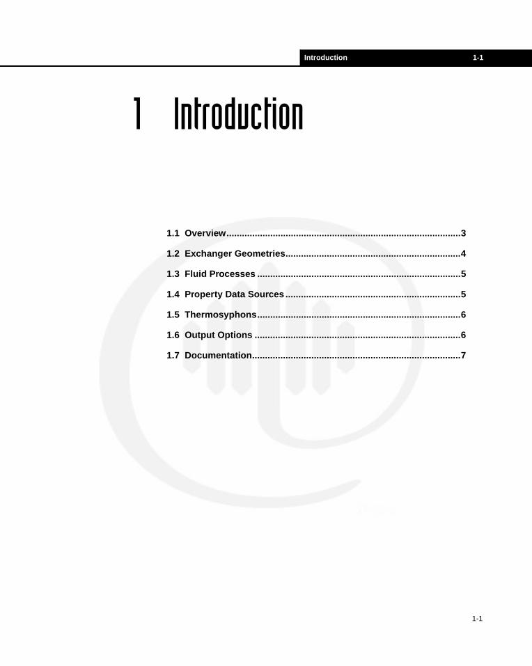
Introduction 1-1

1 Introduction

1-1

1.1 Overview...........................................................................................3

1.2 Exchanger Geometries....................................................................4

1.3 Fluid Processes ...............................................................................5

1.4 Property Data Sources ....................................................................5

1.5 Thermosyphons...............................................................................6

1.6 Output Options ................................................................................6

1.7 Documentation.................................................................................7

1-2 Introduction

1-2

Introduction 1-3

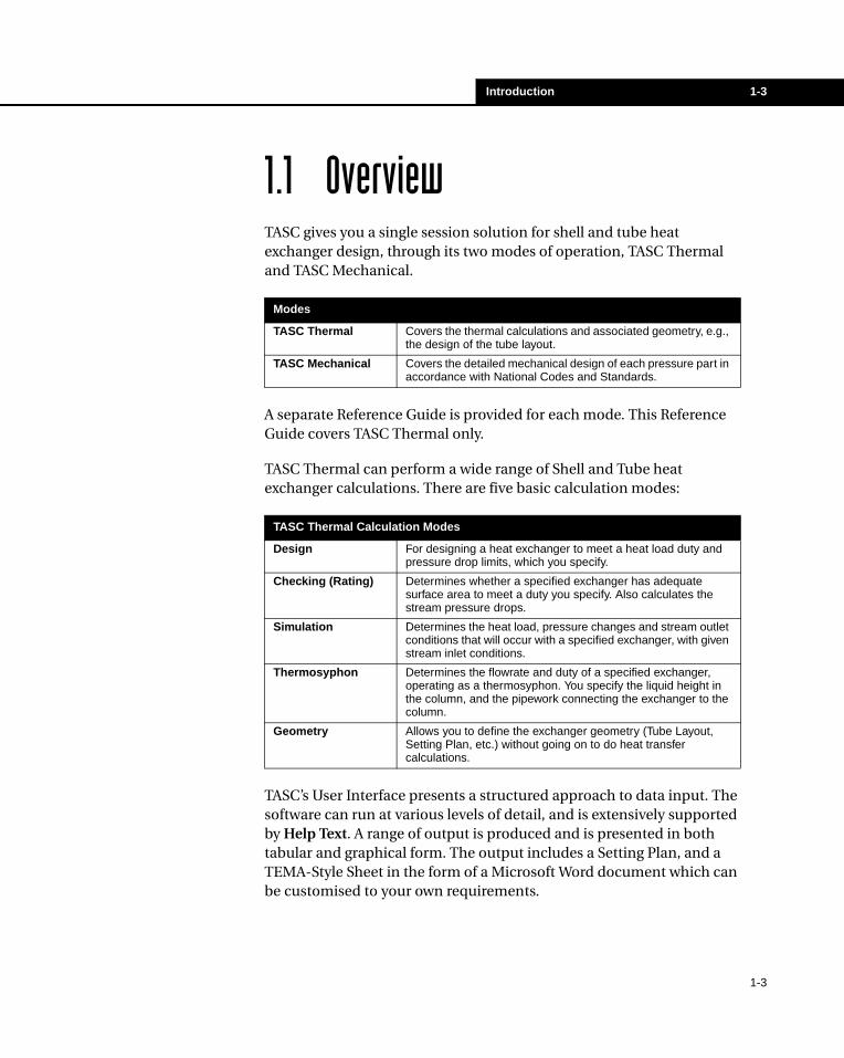
1.1 OverviewTASC gives you a single session solution for shell and tube heat exchanger design, through its two modes of operation, TASC Thermal and TASC Mechanical.

A separate Reference Guide is provided for each mode. This Reference Guide covers TASC Thermal only.

TASC Thermal can perform a wide range of Shell and Tube heat exchanger calculations. There are five basic calculation modes:

TASC’s User Interface presents a structured approach to data input. The software can run at various levels of detail, and is extensively supported by Help Text. A range of output is produced and is presented in both tabular and graphical form. The output includes a Setting Plan, and a TEMA-Style Sheet in the form of a Microsoft Word document which can be customised to your own requirements.

Modes

TASC Thermal Covers the thermal calculations and associated geometry, e.g., the design of the tube layout.

TASC Mechanical Covers the detailed mechanical design of each pressure part in accordance with National Codes and Standards.

TASC Thermal Calculation Modes

Design For designing a heat exchanger to meet a heat load duty and pressure drop limits, which you specify.

Checking (Rating) Determines whether a specified exchanger has adequate surface area to meet a duty you specify. Also calculates the stream pressure drops.

Simulation Determines the heat load, pressure changes and stream outlet conditions that will occur with a specified exchanger, with given stream inlet conditions.

Thermosyphon Determines the flowrate and duty of a specified exchanger, operating as a thermosyphon. You specify the liquid height in the column, and the pipework connecting the exchanger to the column.

Geometry Allows you to define the exchanger geometry (Tube Layout, Setting Plan, etc.) without going on to do heat transfer calculations.

1-3

1-4 Exchanger Geometries

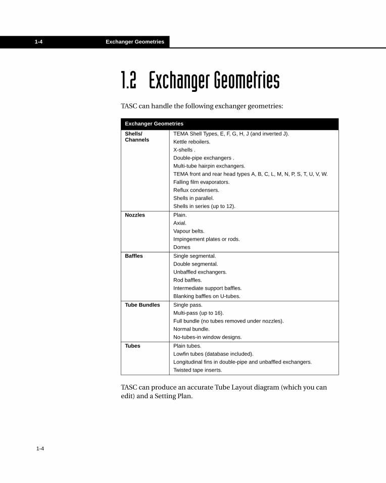
1.2 Exchanger Geometries TASC can handle the following exchanger geometries:

TASC can produce an accurate Tube Layout diagram (which you can edit) and a Setting Plan.

Exchanger Geometries

Shells/Channels

TEMA Shell Types, E, F, G, H, J (and inverted J).

Kettle reboilers.

X-shells .

Double-pipe exchangers .

Multi-tube hairpin exchangers.

TEMA front and rear head types A, B, C, L, M, N, P, S, T, U, V, W.

Falling film evaporators.

Reflux condensers.

Shells in parallel.

Shells in series (up to 12).

Nozzles Plain.

Axial.

Vapour belts.

Impingement plates or rods.

Domes

Baffles Single segmental.

Double segmental.

Unbaffled exchangers.

Rod baffles.

Intermediate support baffles.

Blanking baffles on U-tubes.

Tube Bundles Single pass.

Multi-pass (up to 16).

Full bundle (no tubes removed under nozzles).

Normal bundle.

No-tubes-in window designs.

Tubes Plain tubes.

Lowfin tubes (database included).

Longitudinal fins in double-pipe and unbaffled exchangers.

Twisted tape inserts.

1-4

Introduction 1-5

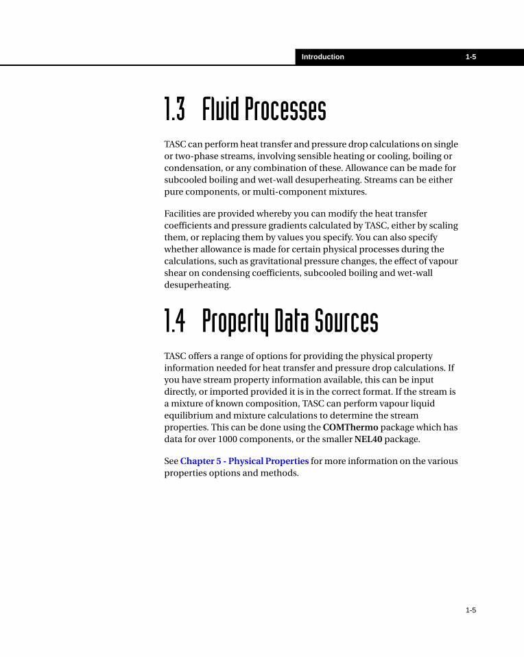
1.3 Fluid ProcessesTASC can perform heat transfer and pressure drop calculations on single or two-phase streams, involving sensible heating or cooling, boiling or condensation, or any combination of these. Allowance can be made for subcooled boiling and wet-wall desuperheating. Streams can be either pure components, or multi-component mixtures.

Facilities are provided whereby you can modify the heat transfer coefficients and pressure gradients calculated by TASC, either by scaling them, or replacing them by values you specify. You can also specify whether allowance is made for certain physical processes during the calculations, such as gravitational pressure changes, the effect of vapour shear on condensing coefficients, subcooled boiling and wet-wall desuperheating.

1.4 Property Data Sources TASC offers a range of options for providing the physical property information needed for heat transfer and pressure drop calculations. If you have stream property information available, this can be input directly, or imported provided it is in the correct format. If the stream is a mixture of known composition, TASC can perform vapour liquid equilibrium and mixture calculations to determine the stream properties. This can be done using the COMThermo package which has data for over 1000 components, or the smaller NEL40 package.

See Chapter 5 - Physical Properties for more information on the various properties options and methods.

1-5

1-6 Thermosyphons

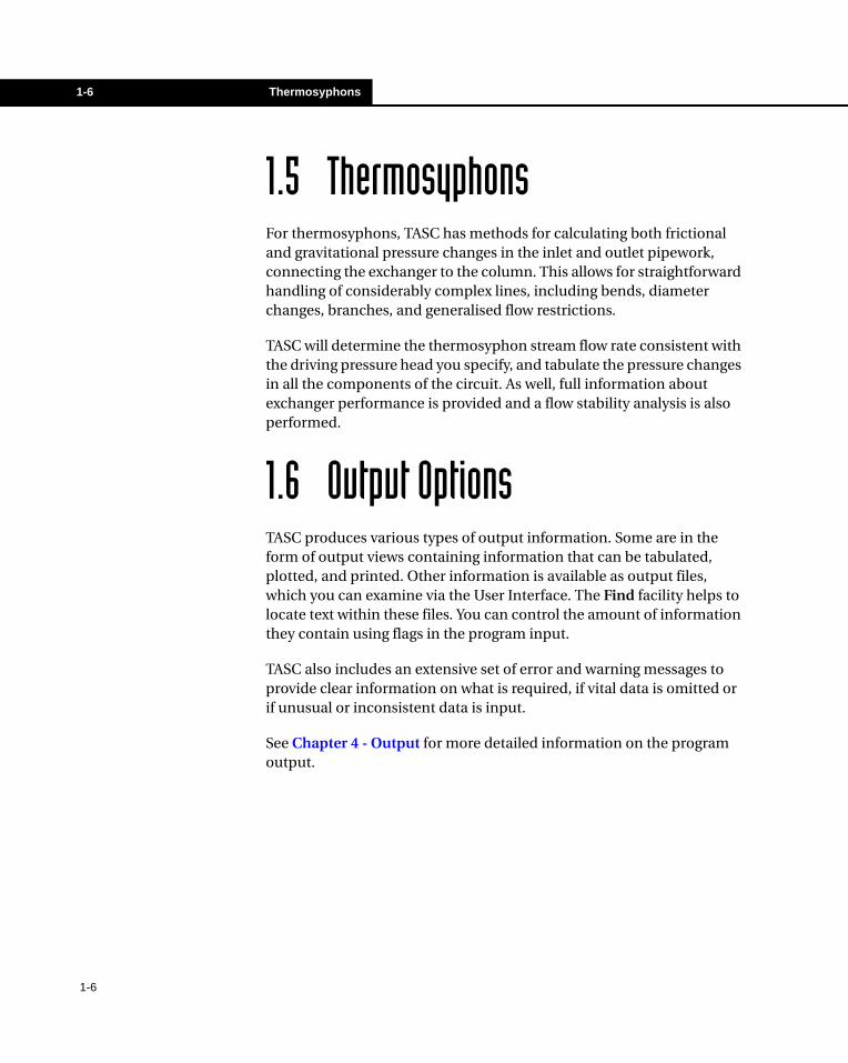
1.5 ThermosyphonsFor thermosyphons, TASC has methods for calculating both frictional and gravitational pressure changes in the inlet and outlet pipework, connecting the exchanger to the column. This allows for straightforward handling of considerably complex lines, including bends, diameter changes, branches, and generalised flow restrictions.

TASC will determine the thermosyphon stream flow rate consistent with the driving pressure head you specify, and tabulate the pressure changes in all the components of the circuit. As well, full information about exchanger performance is provided and a flow stability analysis is also performed.

1.6 Output OptionsTASC produces various types of output information. Some are in the form of output views containing information that can be tabulated, plotted, and printed. Other information is available as output files, which you can examine via the User Interface. The Find facility helps to locate text within these files. You can control the amount of information they contain using flags in the program input.

TASC also includes an extensive set of error and warning messages to provide clear information on what is required, if vital data is omitted or if unusual or inconsistent data is input.

See Chapter 4 - Output for more detailed information on the program output.

1-6

Introduction 1-7

1.7 DocumentationHTFS supplies the following manuals on the HTFS CD:

• HTFS User Guide• HTFS Installation Guide• TASC Getting Started• TASC Reference Guide

For TASC there are separate Getting Started and Reference Guide for TASC Thermal and TASC Mechanical.

This Reference Guide provides basic information on using the program, its capabilities, the required input data (see Chapter 3 - Data Input), and the results (see Chapter 4 - Output). Chapter 5 - Physical Properties covers the range of options for providing the information needed to run the program.

Also contained in this manual is a set of standard examples (see Chapter 7 - Examples) for you to work through. These examples illustrate a range of shell and tube configurations that can be solved using TASC, and show you the various methods of inputting the relevant data.

When appropriate, this manual includes the TASC input and output views to help with explanations. Since TASC is being continuously developed, there may be minor discrepancies between what you see on your computer, and the views shown in this manual. The discrepancies may relate to layout, or to numerical values, but should not be taken as indicating any problem.

See the TASC Getting Started for information on the set of QA data that is included with the program. The QA data are input data sets to help ensure that TASC is functioning properly. These sets should be run in TASC and then checked that the results are the same (within the limits of computer accuracy) as the corresponding output files, which are also provided.

1-7

1-8 Documentation

The Help Text is the most extensive documentation available for TASC. It is available whenever you are running the program, or can be loaded separately. There are direct links to appropriate Help topics for every input item, and from many other places in the program.

The technical methods used in TASC are proprietary, and full details are available only to companies who are full members of the HTFS Research Network. These methods are described in HTFS Design Report DR12.

To load the Help Text when you are not running TASC, double-click on TASC.HLP in the main TASC directory.

1-8

Using TASC 2-1

2 Using TASC

2-1

2.1 Overview...........................................................................................3

2.2 Starting TASC...................................................................................4

2.3 The Start up View.............................................................................6

2.4 Running TASC..................................................................................7

2.5 TASC Icons.......................................................................................8

2-2 Using TASC

2-2

Using TASC 2-3

2.1 OverviewThe normal TASC Thermal run procedure involves setting up the input data representing a particular case, running the case and then examining the results. If you open a case you have previously run, you can examine the results without needing to run the program again. Changes can easily be made to a case and then re-run. You can examine the results of a changed case before deciding to save those changes. A case can be saved with incomplete data and then be re-opened for completion.

Facilities are provided to provide a descriptive title for each run, to specify a run number, and to add a number of lines of comments giving further information.

See Chapter 3 - Data Input for a detailed description of the data input and for output see Chapter 4 - Output. Extensive Help Text is available when running the program. The Help Text covers not only the details of input and output, but also the particulars of the User Interface and about Shell and Tube Exchangers in general.

2-3

2-4 Starting TASC

2.2 Starting TASCClick the Start menu, then Programs, then HTFS, and then TASC. Alternatively, use Windows Explorer or My Computer to select the HTFS\TASC510 folder and double-click on TASC.EXE.

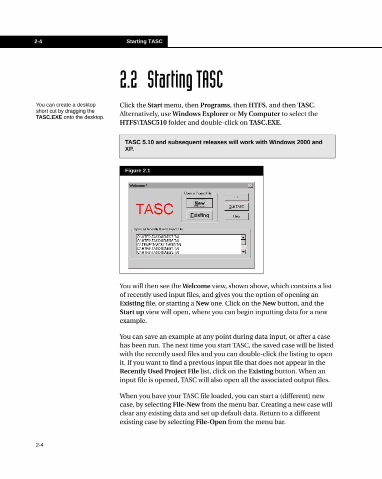
You will then see the Welcome view, shown above, which contains a list of recently used input files, and gives you the option of opening an Existing file, or starting a New one. Click on the New button, and the Start up view will open, where you can begin inputting data for a new example.

You can save an example at any point during data input, or after a case has been run. The next time you start TASC, the saved case will be listed with the recently used files and you can double-click the listing to open it. If you want to find a previous input file that does not appear in the Recently Used Project File list, click on the Existing button. When an input file is opened, TASC will also open all the associated output files.

When you have your TASC file loaded, you can start a (different) new case, by selecting File-New from the menu bar. Creating a new case will clear any existing data and set up default data. Return to a different existing case by selecting File-Open from the menu bar.

TASC 5.10 and subsequent releases will work with Windows 2000 and XP.

Figure 2.1

You can create a desktop short cut by dragging the TASC.EXE onto the desktop.

2-4

Using TASC 2-5

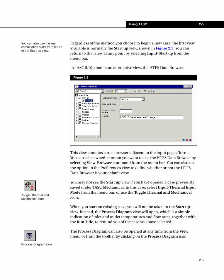
Regardless of the method you choose to begin a new case, the first view available is normally the Start up view, shown in Figure 2.3. You can return to that view at any point by selecting Input-Start up from the menu bar.

In TASC 5.10, there is an alternative view, the HTFS Data Browser.

This view contains a tree browser adjacent to the input pages/forms. You can select whether or not you want to use the HTFS Data Browser by selecting View-Browser command from the menu bar. You can also use the option in the Preferences view to define whether or not the HTFS Data Browser is your default view.

You may not see the Start up view if you have opened a case previously saved under TASC Mechanical. In this case, select Input-Thermal Input Mode from the menu bar, or use the Toggle Thermal and Mechanical icon.

When you start an existing case, you will not be taken to the Start up view. Instead, the Process Diagram view will open, which is a simple indication of inlet and outlet temperatures and flow rates, together with the Run Title, to remind you of the case you have selected.

The Process Diagram can also be opened at any time from the View menu or from the toolbar by clicking on the Process Diagram icon.

Figure 2.2

You can also use the key combination SHIFT F1 to return to the Start up view.

Toggle Thermal and Mechanical icon

Process Diagram icon

2-5

2-6 The Start up View

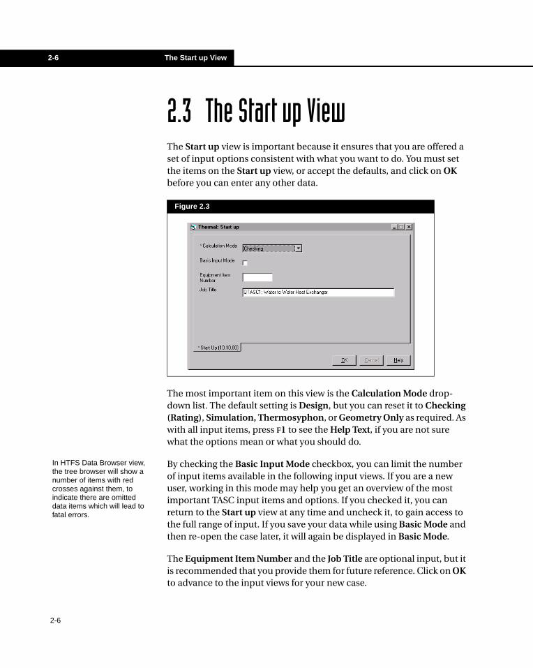
2.3 The Start up ViewThe Start up view is important because it ensures that you are offered a set of input options consistent with what you want to do. You must set the items on the Start up view, or accept the defaults, and click on OK before you can enter any other data.

The most important item on this view is the Calculation Mode drop-down list. The default setting is Design, but you can reset it to Checking (Rating), Simulation, Thermosyphon, or Geometry Only as required. As with all input items, press F1 to see the Help Text, if you are not sure what the options mean or what you should do.

By checking the Basic Input Mode checkbox, you can limit the number of input items available in the following input views. If you are a new user, working in this mode may help you get an overview of the most important TASC input items and options. If you checked it, you can return to the Start up view at any time and uncheck it, to gain access to the full range of input. If you save your data while using Basic Mode and then re-open the case later, it will again be displayed in Basic Mode.

The Equipment Item Number and the Job Title are optional input, but it is recommended that you provide them for future reference. Click on OK to advance to the input views for your new case.

Figure 2.3

In HTFS Data Browser view, the tree browser will show a number of items with red crosses against them, to indicate there are omitted data items which will lead to fatal errors.

2-6

Using TASC 2-7

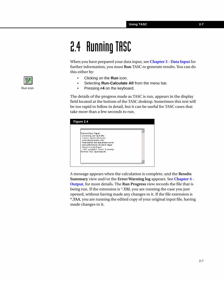
2.4 Running TASCWhen you have prepared your data input, see Chapter 3 - Data Input for further information, you must Run TASC to generate results. You can do this either by:

• Clicking on the Run icon.• Selecting Run-Calculate All from the menu bar.• Pressing F4 on the keyboard.

The details of the progress made as TASC is run, appears in the display field located at the bottom of the TASC desktop. Sometimes this text will be too rapid to follow in detail, but it can be useful for TASC cases that take more than a few seconds to run.

A message appears when the calculation is complete, and the Results Summary view and/or the Error/Warning log appears. See Chapter 4 - Output, for more details. The Run Progress view records the file that is being run. If the extension is *.TAI, you are running the case you just opened, without having made any changes to it. If the file extension is *.TAA, you are running the edited copy of your original input file, having made changes to it.

Figure 2.4

Run icon

2-7

2-8 TASC Icons

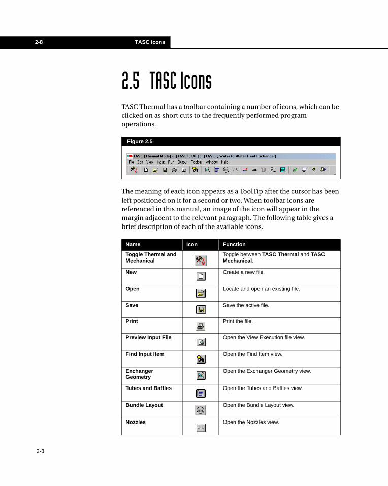
2.5 TASC IconsTASC Thermal has a toolbar containing a number of icons, which can be clicked on as short cuts to the frequently performed program operations.

The meaning of each icon appears as a ToolTip after the cursor has been left positioned on it for a second or two. When toolbar icons are referenced in this manual, an image of the icon will appear in the margin adjacent to the relevant paragraph. The following table gives a brief description of each of the available icons.

Figure 2.5

Name Icon Function

Toggle Thermal and Mechanical

Toggle between TASC Thermal and TASC Mechanical.

New Create a new file.

Open Locate and open an existing file.

Save Save the active file.

Print Print the file.

Preview Input File Open the View Execution file view.

Find Input Item Open the Find Item view.

Exchanger Geometry

Open the Exchanger Geometry view.

Tubes and Baffles Open the Tubes and Baffles view.

Bundle Layout Open the Bundle Layout view.

Nozzles Open the Nozzles view.

2-8

Using TASC 2-9

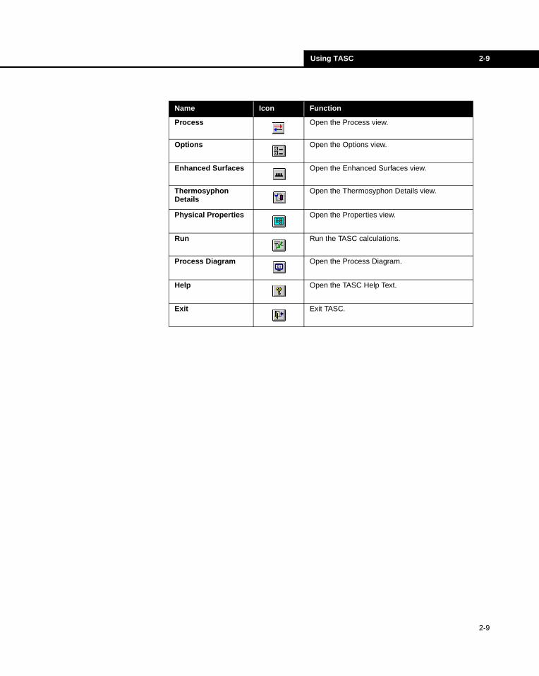
Process Open the Process view.

Options Open the Options view.

Enhanced Surfaces Open the Enhanced Surfaces view.

Thermosyphon Details

Open the Thermosyphon Details view.

Physical Properties Open the Properties view.

Run Run the TASC calculations.

Process Diagram Open the Process Diagram.

Help Open the TASC Help Text.

Exit Exit TASC.

Name Icon Function

2-9

2-10 TASC Icons

2-10

Data Input 3-1

3 Data Input

3-1

3.1 Overview...........................................................................................3

3.2 Input Views.......................................................................................4

3.3 TEMA Input.......................................................................................6

3.4 Process Data Input ..........................................................................7

3.5 Geometry Data Input .......................................................................8

3.6 Other Data Input...............................................................................9

3.7 Input Units ......................................................................................10

3.8 Using Help ......................................................................................12

3.9 Finding Input Items........................................................................13

3.10 The Input File ...............................................................................14

3.11 Default Input Data File.................................................................15

3.12 Input Errors and Warnings..........................................................16

3.13 Tube Layout..................................................................................17

3-2 Data Input

3-2

Data Input 3-3

3.1 OverviewTASC has a number of data input views, each comprising several tabs. You can access these views via the Input menu. The contents of each page may vary slightly according to the Calculation Type (Design, Checking, Simulation, Thermosyphon, or Geometry Only) you have specified.

Data is input by either typing in values, or selecting an option from a drop-down list. You do not need to fill in all the data input items, only those that sufficiently describe the case under consideration.

Many TASC input items have defaults. Most of these defaults are indicated in red on their input form. In many cases they will depend on context and other input values, and are shown as they will be when you Run TASC.

If you are unsure what a data item means, position the cursor on that item and press F1. You will be shown the Help Text on that item, which can show diagrams, define defaults, and let you explore other relevant information. It can point you to more information on why particular design features of shell and tube exchangers are used, or on what use is made of an input item during TASC calculations.

For a full description of each item and a listing of all possible items, use the Help Text. For more information on Physical Properties, both input and output, see Chapter 5 - Physical Properties.

Every time you enter or change an input item, all values are automatically re-checked, and defaults re-set. A record of the items affected is given in the Status Window, at the bottom left of the desktop. For a full check on input, Run TASC. You will immediately see a list of any errors and warnings produced.

A blue background to any input item indicates that it is necessary to supply this item. A yellow background indicates that the item may need attention for correct operation. A red background indicates an error with the input.

Each of these colours can be configured using preferences.

3-3

3-4 Input Views

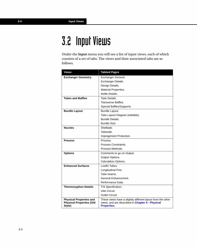
3.2 Input ViewsUnder the Input menu you will see a list of input views, each of which consists of a set of tabs. The views and their associated tabs are as follows.

Views Tabbed Pages

Exchanger Geometry Exchanger General.

Exchanger Details.

Design Details.

Material Properties.

Kettle Details.

Tubes and Baffles Tube Details.

Transverse Baffles.

Special Baffles/Supports

Bundle Layout Bundle Layout.

Tube Layout Diagram (editable).

Bundle Details.

Bundle Size.

Nozzles Shellside.

Tubeside.

Impingement Protection.

Process Process.

Process Constraints.

Process Methods.

Options Comments to go on Output.

Output Options.

Calculation Options.

Enhanced Surfaces Lowfin Tubes.

Longitudinal Fins.

Tube Inserts.

General Enhancement.

Performance Data.

Thermosyphon Details T/S Specification.

Inlet Circuit.

Outlet Circuit.

Physical Properties and Physical Properties (Old Style)

These views have a slightly different layout from the other views, and are described in Chapter 5 - Physical Properties.

3-4

Data Input 3-5

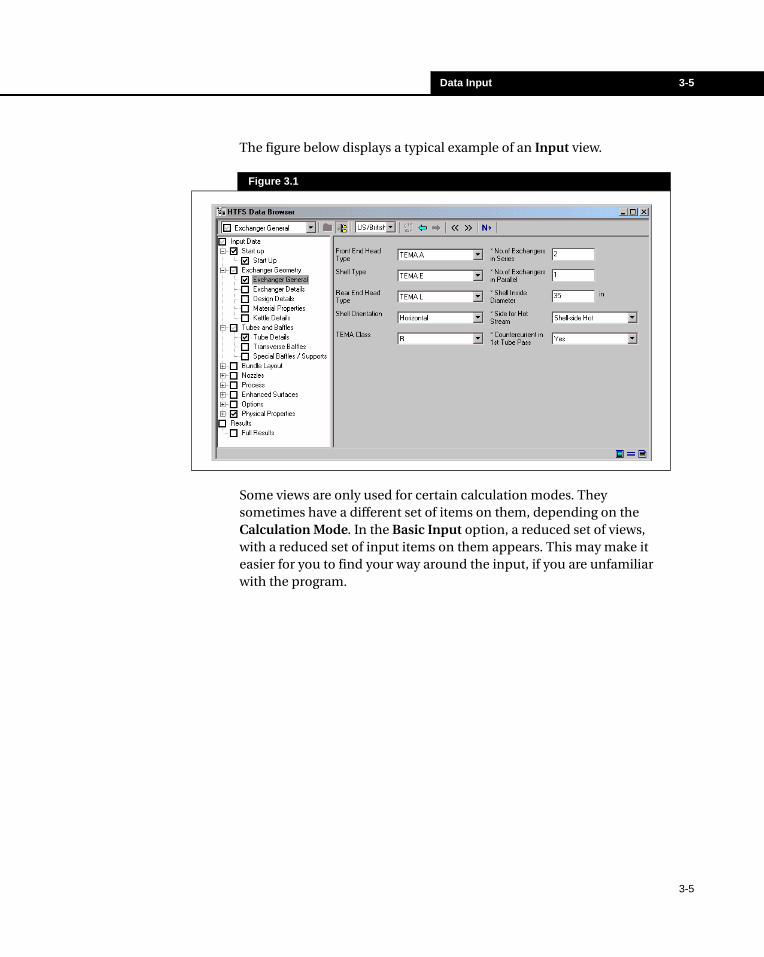
The figure below displays a typical example of an Input view.

Some views are only used for certain calculation modes. They sometimes have a different set of items on them, depending on the Calculation Mode. In the Basic Input option, a reduced set of views, with a reduced set of input items on them appears. This may make it easier for you to find your way around the input, if you are unfamiliar with the program.

Figure 3.1

3-5

3-6 TEMA Input

3.3 TEMA InputThe TEMA Input Form is a alternative input form, which has the standard layout established by TEMA, the Tubular Exchangers Manufacturers Association. If you are familiar with this sheet, you may find it a simpler method of providing the main input than the main TASC views. You will still need to provide some information on the main TASC input views, particularly properties information. You should also specify, on the Exchanger General property view, whether the Shellside or Tubeside is to be the Hot stream, before selecting the TEMA sheet.

Any input supplied to the TEMA Form is transferred directly to the main TASC input views, and vice versa.

The TEMA Form can also be selected from the Output menu, after you have run the TASC calculations, and it will display calculated values, as well as your input.

The TEMA Input Form can be accessed from the Input menu.

3-6

Data Input 3-7

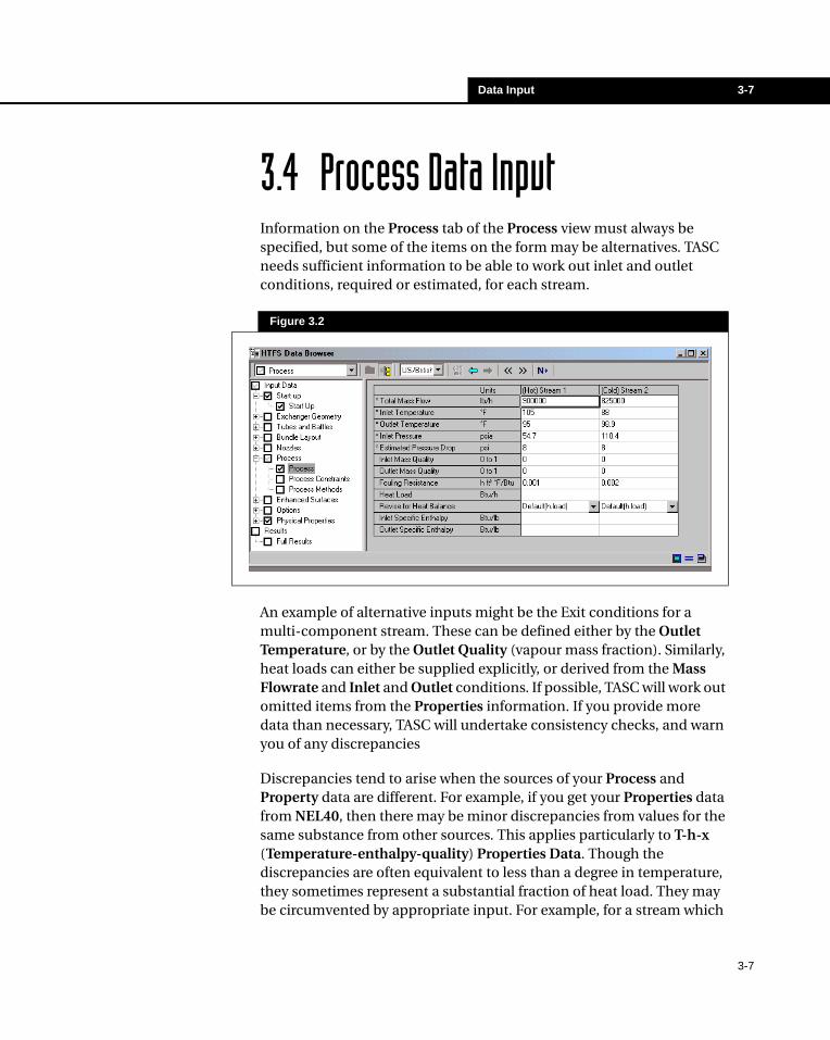
3.4 Process Data InputInformation on the Process tab of the Process view must always be specified, but some of the items on the form may be alternatives. TASC needs sufficient information to be able to work out inlet and outlet conditions, required or estimated, for each stream.

An example of alternative inputs might be the Exit conditions for a multi-component stream. These can be defined either by the Outlet Temperature, or by the Outlet Quality (vapour mass fraction). Similarly, heat loads can either be supplied explicitly, or derived from the Mass Flowrate and Inlet and Outlet conditions. If possible, TASC will work out omitted items from the Properties information. If you provide more data than necessary, TASC will undertake consistency checks, and warn you of any discrepancies

Discrepancies tend to arise when the sources of your Process and Property data are different. For example, if you get your Properties data from NEL40, then there may be minor discrepancies from values for the same substance from other sources. This applies particularly to T-h-x (Temperature-enthalpy-quality) Properties Data. Though the discrepancies are often equivalent to less than a degree in temperature, they sometimes represent a substantial fraction of heat load. They may be circumvented by appropriate input. For example, for a stream which

Figure 3.2

3-7

3-8 Geometry Data Input

must condense completely, it may be best to specify the Outlet Quality (=0.0) rather than the Outlet Temperature, which may not correspond exactly to the Bubble Point Temperature from internal VLE and NEL40 calculations.

Process Data can also be imported, along with Properties Data, from a PSF file. See Chapter 5 - Physical Properties. In such cases data consistency should not be a problem.

The Process Constraints and Process Methods views require input only if you want to make special modifications to the calculations performed.

3.5 Geometry Data InputA large number of input views relate to the geometric configuration of the exchanger and related equipment. Several are only required in special circumstances. The Thermosyphon property view is only required for Themosyphon calculations. The Enhanced Surfaces property view is not needed for exchangers with plain tubes.

The main difference in geometry input is between Design mode calculation and the other calculation modes. In the other modes, you should generally specify as much information as is available to describe the exchanger, in terms of both its size and layout. A number of items have defaults, for example from TEMA recommendations, or can be estimated. Even for such items, it is best to input all the information you have available. If you are unsure whether an item is important or has a default, press F1 to see its Help Text.

For Design calculations, less input is needed. You need to select the basic Exchanger Configuration, such as Shell and Header types, and the Tube Size and Layout. You also need to specify any enhanced surface to be used, and any special baffle type. TASC then determines all the other geometric features, such as shell size and tube length, number of tubes and tubeside passes, the number of exchangers in series and parallel, the size of nozzles, baffles, clearances and so on.

If you are unsure about any of the key items you need to select for a design, the Help Text provides information on when and why various design features are used.

3-8

Data Input 3-9

When you look at the input views in Design mode, you will see that there is the possibility of specifying more data than the basic minimum. Some of this relates to the range of tube lengths, shell diameters etc. that should be explored. Other input items let you preset various features, such as nozzle sizes or baffle cut, to help you constrain the design to meet your particular requirements.

When you run Checking, Simulation, Thermosyphon, or Geometry Only modes, TASC will perform a rigorous Tube Layout Design. A drawing of the Tube Layout will be displayed and you will have the option to edit the Tube Layout. See Section 3.13 - Tube Layout.

Once you have created a Tube Bundle Layout Diagram, you have options which include making it part of the Input, or creating it anew when you next run. If you elect to make it part of the input, you gain access to powerful editing facilities, which allow you to very closely match the layout in the exchanger you are modelling. Any changes you make are then taken (as far as possible) into account during TASC's thermal calculations.

3.6 Other Data InputProperties information must always be provided. This is described in Chapter 5 - Physical Properties.

Options input can normally be set to default values, unless you want to modify the basis of the calculations, or suppress or switch on certain outputs.

3-9

3-10 Input Units

3.7 Input UnitsThere are three pre-defined unit sets available in TASC:

• SI (mm, °C, kJ/kg etc.)• British/US customary (inches, °F, BTU/lb etc.)• Metric (mm, °C, kCal/kg etc.)

The Geometry and Process Data can be defined using different unit sets within a single case. Properties Data can be defined with different unit sets for every individual stream.

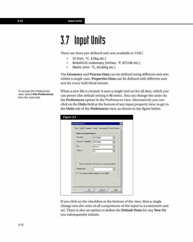
When a new file is created, it uses a single unit set for all data, which you can preset (the default setting is SI units). You can change the units via the Preferences option in the Preferences view. Alternatively you can click on the Units field at the bottom of any input property view, to get to the Units tab of the Preferences view, as shown in the figure below.

If you click on the checkbox at the bottom of the view, then a single change sets the units of all components of the input to a consistent unit set. There is also an option to define the Default Units for any New file you subsequently initiate.

Figure 3.3

To access the Preferences view, select File-Preferences from the menu bar.

3-10

Data Input 3-11

You cannot modify the individual units setting for the Stream or Component input via the Preferences view. This must be done directly on the Physical Property Data view. However, if the checkbox at the bottom of the view is checked, than changing any of the other unit sets will automatically change the unit sets for these items, as well.

When you change the units, you can decide whether or not any values you have already input should have their units converted to the new system.

The program output units will be deduced from the input units, though you can explicitly specify one of the three sets on the Output tab of the Output view.

Some of the preset defaults in the Geometry input have units, so you should select the Convert option even if you have not yet supplied any data.

3-11

3-12 Using Help

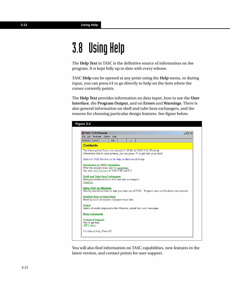
3.8 Using HelpThe Help Text in TASC is the definitive source of information on the program. It is kept fully up to date with every release.

TASC Help can be opened at any point using the Help menu, or during input, you can press F1 to go directly to help on the item where the cursor currently points.

The Help Text provides information on data input, how to use the User Interface, the Program Output, and on Errors and Warnings. There is also general information on shell and tube heat exchangers, and the reasons for choosing particular design features. See figure below.

You will also find information on TASC capabilities, new features in the latest version, and contact points for user support.

Figure 3.4

3-12

Data Input 3-13

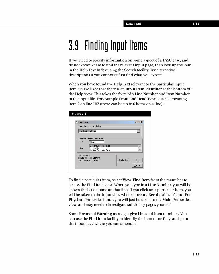
3.9 Finding Input ItemsIf you need to specify information on some aspect of a TASC case, and do not know where to find the relevant input page, then look up the item in the Help Text Index using the Search facility. Try alternative descriptions if you cannot at first find what you expect.

When you have found the Help Text relevant to the particular input item, you will see that there is an Input Item Identifier at the bottom of the Help view. This takes the form of a Line Number and Item Number in the input file. For example Front End Head Type is 102.2, meaning item 2 on line 102 (there can be up to 6 items on a line).

To find a particular item, select View-Find Item from the menu bar to access the Find Item view. When you type in a Line Number, you will be shown the list of items on that line. If you click on a particular item, you will be taken to the input view where it occurs. See the above figure. For Physical Properties input, you will just be taken to the Main Properties view, and may need to investigate subsidiary pages yourself.

Some Error and Warning messages give Line and Item numbers. You can use the Find Item facility to identify the item more fully, and go to the input page where you can amend it.

Figure 3.5

3-13

3-14 The Input File

3.10 The Input FileWhen you provide TASC input, it is used to generate an input file, which has an essentially simple layout and contains all the information you have provided. The core of the file consists of a set of lines, each identified by a number occupying the first three characters, and followed by up to six items of data. This core information is actually wrapped in XML, containing information relating to the Tube Layout and COMThermo. When only some of the items on a line of core information are present, asterisks (*) are used to indicate omitted items.

The data lines are gathered together into 'blocks', with a related set of line numbers. The following table lists the data type and their respective number ranges.

The first line in each block identifies the block, and the units of the input data. Some data blocks are repeated, for example there is a Process block, and at least one Properties block, for each stream.

A full listing of all possible input data items is given in the Help Text. The Help Text on individual items indicates the line number (and position on the line).

You can preview the Input data file, before it is run, under the View menu.

The User Interface normally holds an internal version of the input file, which is modified in response to changes you make in the input, and which is used when the TASC calculations are Run. You have the option of saving this internal version of the input file, at any stage. You will be explicitly offered the option of saving it each time you Run calculations, or, if you have changed any input items, on Exit from the program. If you do not save it, any initial version of your input file will be left unaltered.

Data Type Range

Geometry 101-199

Process 201-299

Stream Properties 301-399

Component Properties 401-499

Program Options 001-099

3-14

Data Input 3-15

3.11 Default Input Data FileTASC allows you to set up a Default Input Data File, which is called up whenever you begin a New input data file. It can contain any amount of preset input data. You can set up several default input files, and have the option of selecting from among them when you run TASC.

To set up such a default file:

1. Create a partial input data file in the usual way, and save it with an appropriate name.

2. Select File-Preferences from the menu bar to access the Preferences view.

3. In the Preferences view, go to the Files tab.

4. Set your default file under the Default Input File option.

When you use a Default Input File, you should ensure that you use the Save As command (under the File menu) to save new cases. Save your file with a name different than that of your default input file, otherwise this modified file will be saved as the default.

To change the Default Input Data File, go to the Files tab of the Preferences view, and make your selection. Click OK and TASC will use the new file as the default input file for all subsequent cases.

The Component Properties Input (400 series lines) relates to the now deprecated input option, which is only available under OldStyle Physical Properties. COMThermo related information on properties is stored in XML information within the Input File.

3-15

3-16 Input Errors and Warnings

3.12 Input Errors and WarningsIf some mal-operation occurs when you are using the TASC User Interface, or if you have provided data which the Interface cannot interpret, then an Information Message view will appear. You should click on this, and take appropriate action before continuing.

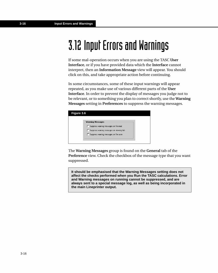
In some circumstances, some of these input warnings will appear repeated, as you make use of various different parts of the User Interface. In order to prevent the display of messages you judge not to be relevant, or to something you plan to correct shortly, use the Warning Messages setting in Preferences to suppress the warning messages.

The Warning Messages group is found on the General tab of the Preference view. Check the checkbox of the message type that you want suppressed.

Figure 3.6

It should be emphasised that the Warning Messages setting does not affect the checks performed when you Run the TASC calculations. Error and Warning messages on running cannot be suppressed, and are always sent to a special message log, as well as being incorporated in the main Lineprinter output.

3-16

Data Input 3-17

3.13 Tube LayoutThe Tube Layout diagram is relevant to all modes of TASC, except Design. The diagram is generated the first time you run a Checking or Simulation case. Once you have a diagram, you can chose either to regenerate it every time you run, or to keep it and use it as a source of input information.

When you use the diagram for Input, it is used to supply values for parameters defaulted in the main Input. You can also edit this diagram to refine or modify it before you Run TASC to perform the required Checking or Simulation calculation of the exchanger. In Geometry Only mode, the appearance of this diagram is effectively the end of the calculation.

You can edit the Tube Layout diagram to Add or Delete various features, or you can move them using a ‘nudge’ facility or by revising the values for their location in an accompanying spreadsheet.

Messages are produced whenever there are inconsistencies between the Tube Layout diagram and other input values you have specified. When you save a TASC case, the Tube Layout diagram is also saved, so it is available when you re-open the case.

3-17

3-18 Tube Layout

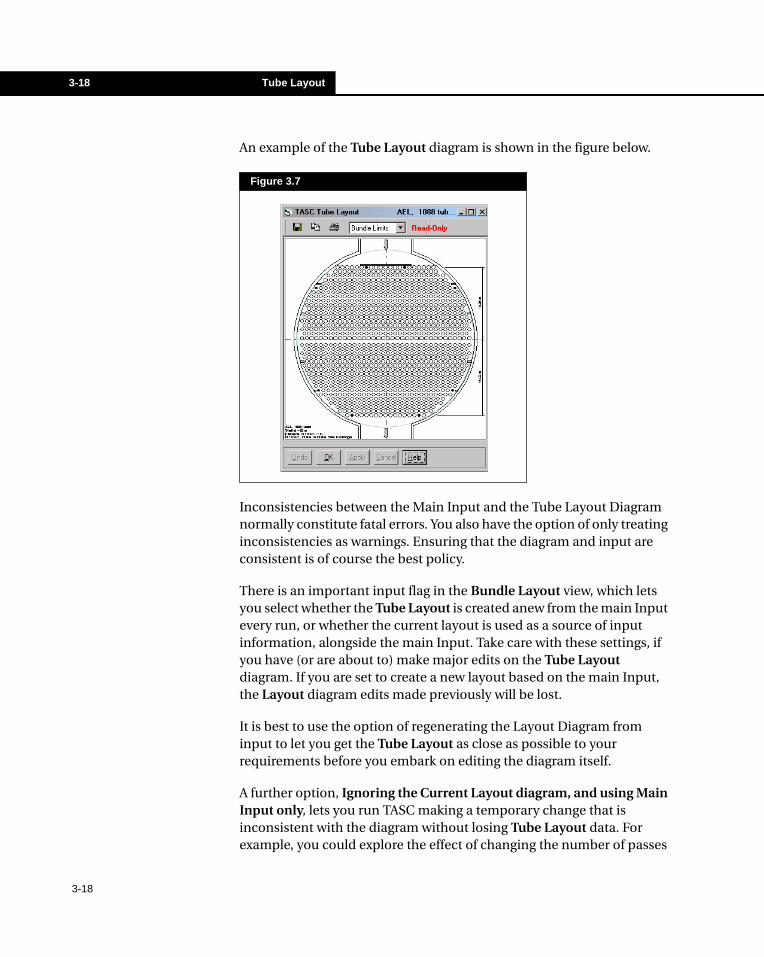
An example of the Tube Layout diagram is shown in the figure below.

Inconsistencies between the Main Input and the Tube Layout Diagram normally constitute fatal errors. You also have the option of only treating inconsistencies as warnings. Ensuring that the diagram and input are consistent is of course the best policy.

There is an important input flag in the Bundle Layout view, which lets you select whether the Tube Layout is created anew from the main Input every run, or whether the current layout is used as a source of input information, alongside the main Input. Take care with these settings, if you have (or are about to) make major edits on the Tube Layout diagram. If you are set to create a new layout based on the main Input, the Layout diagram edits made previously will be lost.

It is best to use the option of regenerating the Layout Diagram from input to let you get the Tube Layout as close as possible to your requirements before you embark on editing the diagram itself.

A further option, Ignoring the Current Layout diagram, and using Main Input only, lets you run TASC making a temporary change that is inconsistent with the diagram without losing Tube Layout data. For example, you could explore the effect of changing the number of passes

Figure 3.7

3-18

Data Input 3-19

or the tube pattern. When you revert to your original geometry your diagram will still be available.

There is an option on the Bundle Layout input to view the diagram during a run. You can also view the Tube Layout as part of the Output. In either of these cases, you cannot edit the diagram.

3-19

3-20 Tube Layout

3-20

Output 4-1

4 Output

4-1

4.1 Overview...........................................................................................3

4.2 Output Views....................................................................................3

4.3 Output Files......................................................................................6

4.4 Error / Warning Message Log .........................................................8

4.5 Other Output ....................................................................................9

4-2 Output

4-2

Output 4-3

4.1 OverviewRunning the core TASC program produces a number of different types of output. These can be viewed using the Output menu. When you save an example, all the key output files remain in place, so that you can view the output again once you open a case you have previously worked on.

This chapter gives an overview of the various outputs you can inspect to help you find particular details that may be of interest to you. A more detailed description of all the Outputs is available in the Help Text. See Output in the Help Text contents page.

4.2 Output ViewsYou can select from a set of output property views, which contain the main results. These include:

• Thermal Results Summary• Full Results• Nozzles• Integration Along Shell• Alternative designs (available in Design mode only)

Either the Results Summary view or the Full Results view (you can select which under the General tab on the Preferences view) will automatically appear at the end of a run, providing TASC has run successfully. An exception is Geometry mode where the Tube Layout diagram (see Section 4.4 - Error / Warning Message Log) appears at the end of a run.

The Results Summary contains Geometric, Process, and Performance Data. In Design mode, the most important results will be the Geometric information.

To access the Preferences view, select File-Preferences command from the menu bar.

4-3

4-4 Output Views

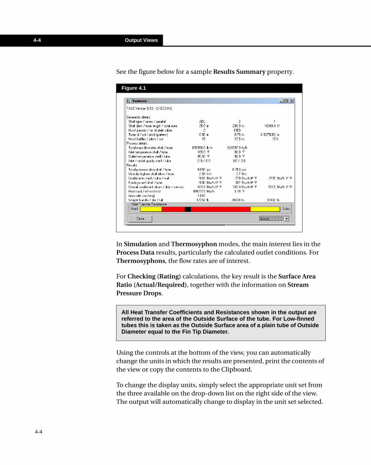
See the figure below for a sample Results Summary property.

In Simulation and Thermosyphon modes, the main interest lies in the Process Data results, particularly the calculated outlet conditions. For Thermosyphons, the flow rates are of interest.

For Checking (Rating) calculations, the key result is the Surface Area Ratio (Actual/Required), together with the information on Stream Pressure Drops.

Using the controls at the bottom of the view, you can automatically change the units in which the results are presented, print the contents of the view or copy the contents to the Clipboard.

To change the display units, simply select the appropriate unit set from the three available on the drop-down list on the right side of the view. The output will automatically change to display in the unit set selected.

Figure 4.1

All Heat Transfer Coefficients and Resistances shown in the output are referred to the area of the Outside Surface of the tube. For Low-finned tubes this is taken as the Outside Surface area of a plain tube of Outside Diameter equal to the Fin Tip Diameter.

4-4

Output 4-5

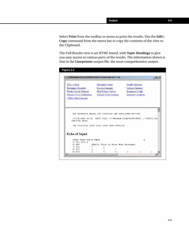
Select Print from the toolbar or menu to print the results. Use the Edit | Copy command from the menu bar to copy the contents of the view to the Clipboard.

The Full Results view is an HTML based, with Topic Headings to give you easy access to various parts of the results. The information shown is that in the Lineprinter output file, the most comprehensive output.

Figure 4.2

4-5

4-6 Output Files

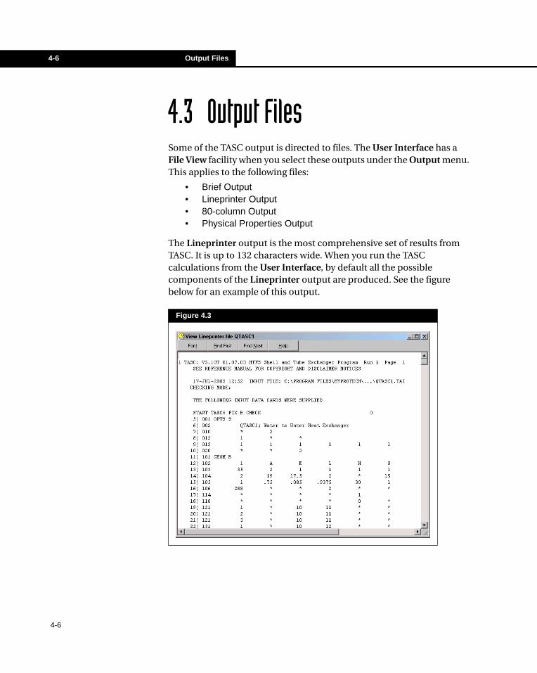
4.3 Output FilesSome of the TASC output is directed to files. The User Interface has a File View facility when you select these outputs under the Output menu. This applies to the following files:

• Brief Output• Lineprinter Output• 80-column Output• Physical Properties Output

The Lineprinter output is the most comprehensive set of results from TASC. It is up to 132 characters wide. When you run the TASC calculations from the User Interface, by default all the possible components of the Lineprinter output are produced. See the figure below for an example of this output.

Figure 4.3

4-6

Output 4-7

The 80-column output is a more restricted version of the Lineprinter output. The Brief output contains similar information to the Results Summary view.

For each of the output file views, four buttons are available at the top of the view. These buttons and their functionality are listed in the following table:

If you would like to limit the information sent to the output files, open the Options view from the Input menu. On the Output Options tab, select No Output from the drop-down lists of any of the data output you do not want. Re-run the program to generate the reduced file.

Button Function

Font Opens a view and allows you to change the file font.

Find Activates the Find operation that will locate a word or phrase you specify, within the file view. Use this operation to quickly locate information on a certain aspect of an exchanger. Simply use a word relevant to the information desired and then the Find operation will locate that text, if it exists, within the file.

Find Next After locating the first occurrence of a text string within the file view using the Find button, use the Find Next button to locate all subsequent occurrences of this text string.

Help Opens a a Viewer Help view.

The Find operation is not case sensitive.

4-7

4-8 Error / Warning Message Log

4.4 Error / Warning Message LogWhen you run TASC calculations, an extensive set of checks is performed on the data you have provided, and then further checks are made as the program continues its operation. These checks may result in Error and Warning messages, which are collected together in a file and which also appear in the main record of the run, the Lineprinter output. The Messages file will be the first thing you see when you have run TASC, if a fatal error has occurred.

Errors are normally fatal, in that TASC has identified some fundamental inconsistency in your data, or a lack of vital data, which means that it cannot continue further with its calculations. If you have used the HTFS Data Browser, and eliminated all the red markings, you would not normally expect to see any such fatal errors. Nevertheless, it is still possible for fatal errors to occur, as TASC proceeds to deeper levels of data checking.

Warnings occur if a value you have supplied is outside an expected range, for example an Inlet Temperature of -100 oC, which is not impossible, but unlikely. Warnings occur if there is an inconsistency in your data, for example if you specify an Inlet Quality which is different from that deduced from your Inlet Temperature. They also occur if your exchanger has some unexpected feature, such as an end-space length less than the Baffle Spacing.

With any such warnings you should check the input data, to confirm that it is as you intended, and amend it if necessary.

Some warnings inform you about phenomena in your exchanger (Dryout, Thermosyphon Stability etc.), or inform you that the conditions in your exchanger are beyond the range of available correlations. In such cases you may need to make an engineering judgement about whether your design, or design margin, is appropriate.

4-8

Output 4-9

4.5 Other OutputWhen TASC is run it produces a file called the Intout file, extension *.TAF, which contains all the data needed by the Output views. From the Interface, you cannot either view this file, or suppress its output.

There are five other special outputs, which can be brought up under the TASC Output menu:

• Report Generator• TEMA Specification Sheet• Word Specification Sheet• Setting Plan• Tube Layout Drawing• Costing Package

The Report Generator lets you produce output with an improved layout, suitable for printing or exporting to other software packages. In this form, it gives access to key parts of the TASC results, in both tabular and graphical format. Information from this form is also available in other parts of the output views.

The TEMA Specification Sheet is the same as can be used for input, as described in Chapter 3 - Data Input, but will display calculated results as well as your input.

The Word Specification Sheet has a similar layout to the TEMA sheet, but is a Word document and can be customised to your company’s requirements. The Word Specification Sheet, the Setting Plan, the Tube Layout Drawing and the Costing Package are all described in Chapter 6 - Other Facilities.

4-9

4-10 Other Output

4-10

Physical Properties 5-1

5 Physical Properties

5-1

5.1 Overview...........................................................................................3

5.1.1 Properties Data Input ...............................................................45.1.2 Properties Used .......................................................................5

5.2 Properties Input ...............................................................................6

5.2.1 Setting a Data Source ..............................................................85.2.2 Get Properties ..........................................................................95.2.3 Rules for Direct Property Input ...............................................10

5.3 Properties Data Input (Old Style) .................................................11

5.3.1 Input Directly ..........................................................................125.3.2 User Databank .......................................................................135.3.3 Single Component Stream from NEL40 .................................145.3.4 Components: Calculation of the Properties of a Mixture........14

5.4 Mixture Calculations (Old Style)...................................................15

5.5 Property Databanks.......................................................................18

5.6 Importing Properties and Process Data ......................................20

5.6.1 Importing PSF Files................................................................20

5.7 Importing from HYSYS..................................................................23

5.8 Importing from Properties Package.............................................24

5.9 Properties Output ..........................................................................25

5.10 Pressure Dependence.................................................................26

5-2 Physical

5-2

Physical Properties 5-3

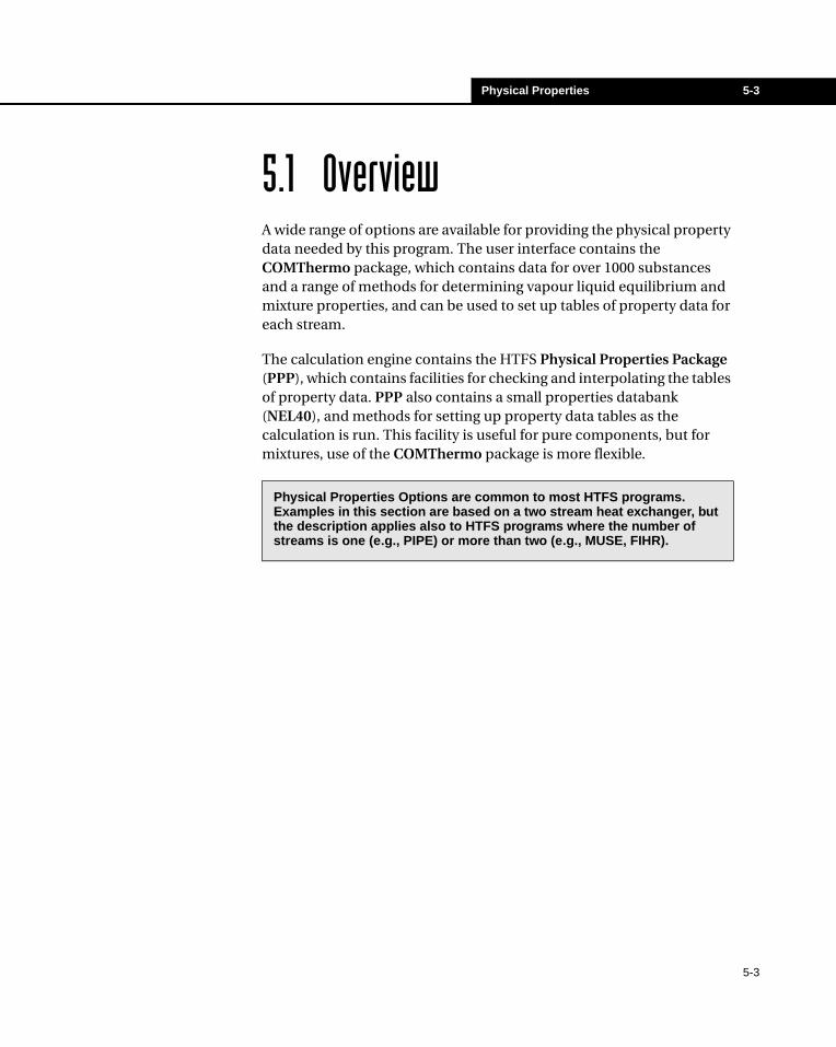
5.1 OverviewA wide range of options are available for providing the physical property data needed by this program. The user interface contains the COMThermo package, which contains data for over 1000 substances and a range of methods for determining vapour liquid equilibrium and mixture properties, and can be used to set up tables of property data for each stream.

The calculation engine contains the HTFS Physical Properties Package (PPP), which contains facilities for checking and interpolating the tables of property data. PPP also contains a small properties databank (NEL40), and methods for setting up property data tables as the calculation is run. This facility is useful for pure components, but for mixtures, use of the COMThermo package is more flexible.

Physical Properties Options are common to most HTFS programs. Examples in this section are based on a two stream heat exchanger, but the description applies also to HTFS programs where the number of streams is one (e.g., PIPE) or more than two (e.g., MUSE, FIHR).

5-3

5-4 Overview

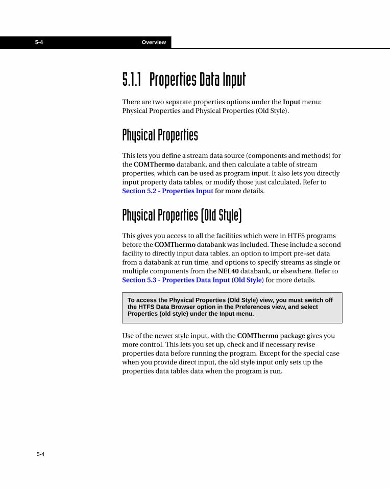
5.1.1 Properties Data Input There are two separate properties options under the Input menu: Physical Properties and Physical Properties (Old Style).

Physical PropertiesThis lets you define a stream data source (components and methods) for the COMThermo databank, and then calculate a table of stream properties, which can be used as program input. It also lets you directly input property data tables, or modify those just calculated. Refer to Section 5.2 - Properties Input for more details.

Physical Properties (Old Style)This gives you access to all the facilities which were in HTFS programs before the COMThermo databank was included. These include a second facility to directly input data tables, an option to import pre-set data from a databank at run time, and options to specify streams as single or multiple components from the NEL40 databank, or elsewhere. Refer to Section 5.3 - Properties Data Input (Old Style) for more details.

Use of the newer style input, with the COMThermo package gives you more control. This lets you set up, check and if necessary revise properties data before running the program. Except for the special case when you provide direct input, the old style input only sets up the properties data tables data when the program is run.

To access the Physical Properties (Old Style) view, you must switch off the HTFS Data Browser option in the Preferences view, and select Properties (old style) under the Input menu.

5-4

Physical Properties 5-5

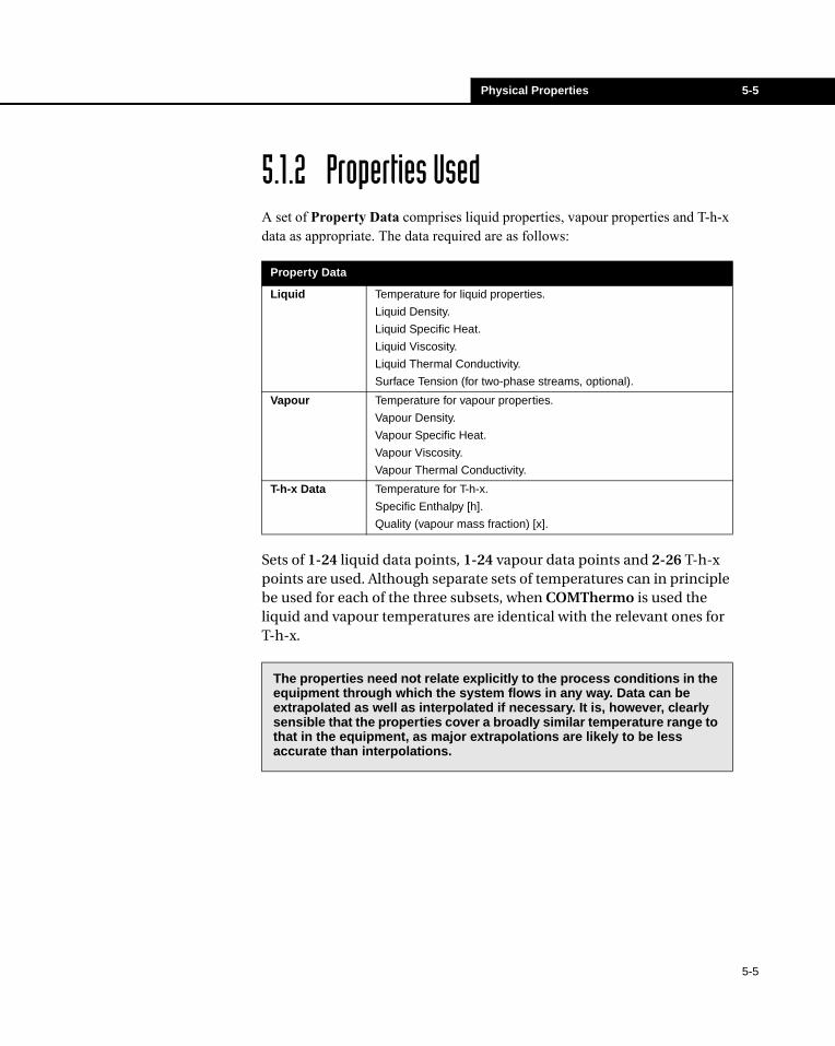
5.1.2 Properties UsedA set of Property Data comprises liquid properties, vapour properties and T-h-x data as appropriate. The data required are as follows:

Sets of 1-24 liquid data points, 1-24 vapour data points and 2-26 T-h-x points are used. Although separate sets of temperatures can in principle be used for each of the three subsets, when COMThermo is used the liquid and vapour temperatures are identical with the relevant ones for T-h-x.

Property Data

Liquid Temperature for liquid properties.

Liquid Density.

Liquid Specific Heat.

Liquid Viscosity.

Liquid Thermal Conductivity.

Surface Tension (for two-phase streams, optional).

Vapour Temperature for vapour properties.

Vapour Density.

Vapour Specific Heat.

Vapour Viscosity.

Vapour Thermal Conductivity.

T-h-x Data Temperature for T-h-x.

Specific Enthalpy [h].

Quality (vapour mass fraction) [x].

The properties need not relate explicitly to the process conditions in the equipment through which the system flows in any way. Data can be extrapolated as well as interpolated if necessary. It is, however, clearly sensible that the properties cover a broadly similar temperature range to that in the equipment, as major extrapolations are likely to be less accurate than interpolations.

5-5

5-6 Properties Input

5.2 Properties InputProperties input using COMThermo normally involves:

• Setting up one or more data Sources.• Selecting a data source for each stream, then defining the

composition, temperatures and pressures for the properties data tables.

• Generating the property data tables, using Get Properties button.

There are, however, four special data sources also provided:

• Direct Input. You type the numbers in yourself, copy them from a spreadsheet, or modify values already calculated by COMThermo. See Section 5.2.1 - Setting a Data Source.

• Not set here. One of the options under Physical Properties (old style) is used. See Section 5.3 - Properties Data Input (Old Style).

• Air or Water from NEL40. A special setting under which air or water data are obtained from the NEL40 package at run time. No further settings for the stream are necessary.

5-6

Physical Properties 5-7

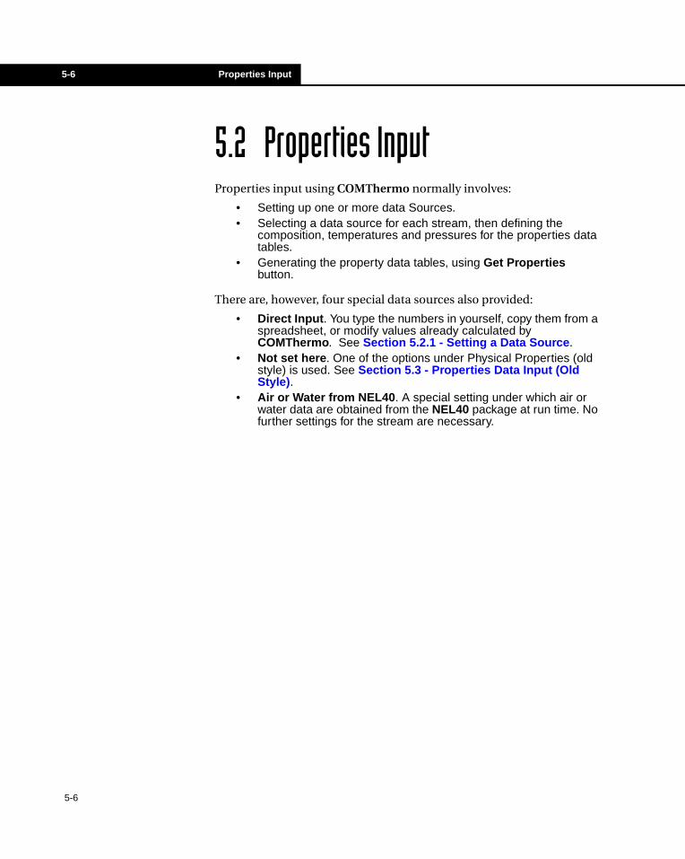
The data source options, and calculated property tables are shown in the main Physical properties view.

Figure 5.1

5-7

5-8 Properties Input

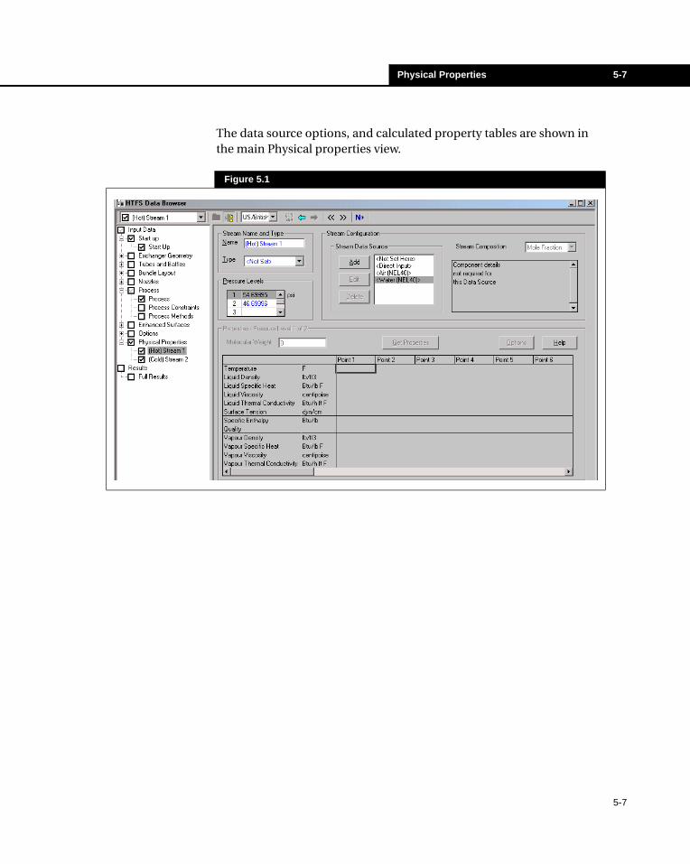
5.2.1 Setting a Data SourceA Data Source defines the components in a stream, and the VLE and properties methods to be used. For a new case you will normally first click on Add to set up a new Data Source. You can then select a set of components from the master list, and add them to the list for the Data Source. A Search facility lets you find components in the list more easily, searching on either name or formula. Many components can be identified under a variety of synonyms. The form ‘*abc’ can be searched on, to find the string ‘abc’ preceded by other characters.

To define a data source, it is necessary to select property calculation methods, (on the Property Package tab) as well as a set of components.

If you selected a Stream Type on the main properties input form, then a default Property Package will be selected. You can, however, change the package used, from a selection including Peng Robinson, SRK, NRTL, and variants on these. A brief description of each is given on the view.

A Property Package effectively defines both a VLE (vapour liquid equilibrium) method for each phase, and a set of methods for subsequently determining the individual properties of each phase. By clicking on the Advanced Views button, you will gain access to facilities

Figure 5.2

5-8

Physical Properties 5-9

which let you select the property method individually for each property for each phase, and gives you further advanced options, such as selecting from a much wider range of VLE methods for each phase, giving control over the convergence criteria for the VLE, and the ability to view and modify the VLE interaction parameters.

When both components and Property Package are set, the status bar at the bottom right turns green and reads Ready. You can then close this view, and on the main Properties input view, the new Data Source is available to be selected for any stream.

5.2.2 Get PropertiesGet Properties calculates properties at one or more pressure levels, using a set of temperature points. Using the Options facility lets you either define a temperature range and a number of points (from which the temperature points are determined automatically) or you can choose to specify the temperatures to be used explicitly. A temperature range and set of pressures are initialised from any process information you provide where possible.

Get Properties causes the spreadsheet of property data to be filled in automatically. If a stream is two phase within or near the range of defined temperatures, property data at the bubble and dew point are added in.

After properties have been calculated you can delete individual data points (data columns). You can explore the effect of changing the Property Package, used using Edit to revise the Data Source.

Once data has been generated, you can change the Data Source to Direct Input and edit individual property values, though this is not recommended.

5-9

5-10 Properties Input

5.2.3 Rules for Direct Property InputData for Two Phase streams must always contain the dew and bubble points, if these points are within the range of data you supply. If they are outside the range of data provided, they will be estimated by extrapolation of T-h-x data. When data are provided, the highest Enthalpy point with Quality 0 is assumed to be the bubble point, and the lowest Enthalpy point with Quality 1 is assumed to be the dew point. Points need not be provided in any particular order, but are sorted into order of increasing enthalpy by the PPP when the calculation is Run.

The facility to supply the specific enthalpy and molecular weight of individual phases is available via the Show Phase Enthalpies and Molecular Weights checkbox, on the Options view. These are always optional inputs.

For Single Phase streams data need only be input for one phase. Specific enthalpy data are optional, as they can be found by integrating specific heats.

A set of Stream Properties data you specify should all relate to the same pressure, typically some mean pressure within the exchanger. You can supply a second set of stream data at a different pressure, permitting the program to allow for the pressure dependence of properties. Such dependence is sometimes significant, particularly for thermosyphons, or if there is a very close temperature approach between streams. For the PIPE program, pressure dependence is mandatory.

Refer to Section 5.10 - Pressure Dependence for more information regarding pressure dependence.

5-10

Physical Properties 5-11

5.3 Properties Data Input (Old Style)The Old Style physical properties input gives access to all the facilities that were present before HTFS programs included the COMThermo. Many of these facilities are associated with the fact that, unlike COMThermo options, with many old-style options you cannot see the properties until you have run the Calculation Engine.

The master view for old style input is shown in the above figure. Using this view, Physical Property information can be supplied in a number of ways.

You can:

• Input Stream Properties directly. You can either type them, or import them from a PSF file. See Section 5.6 - Importing Properties and Process Data.

• Identify data from a User Databank. The calculation engine will read data from this databank when it runs.

• For a single component stream, get the data directly from the NEL40 Databank supplied with the program.

• Tell the program the stream components and composition, and get it to calculate the properties.

Figure 5.3

5-11

5-12 Properties Data Input (Old Style)

The Data Source item on the main Physical Properties input view allows you to select the various options. You should also set the Phase before supplying further data. A two-phase stream means that it can be either single phase or two phase, depending on the temperature.

If you have previously set up properties data using COMThermo, or the corresponding direct input (see Section 5.2 - Properties Input), you will see the Data Source set to Approximately. You can change the Data Source to Direct Input, and view and edit the properties data, but you will not be able to access it again using the main Properties Input.

5.3.1 Input DirectlyIf you set the Data Source to Input Directly, you can then click on the Property Table button to open a view, shown in the figure below, where you can enter the properties.

If you have previously imported data from a PSF file, you will be able to see what you have imported.

Figure 5.4

5-12

Physical Properties 5-13

You need to specify the properties indicated above for one or both phases. For Two-phase streams you also supply T-h-x data. Although you can supply data at up to 24 temperature points, this is potentially tedious if you are typing the data in, and you are most likely to use this method when you have only one or two data points available, for example at an exchanger inlet and outlet.

You can use different sets of temperatures for the Liquid, Two-phase (Enthalpy + Quality) and Vapour Properties. You should normally fill in the data tables from the left, without leaving gaps, though this is not strictly necessary.

For Single Phase streams, T-h-x data are not usually input, as they can be found by integrating specific heats. If, however, you do want to input Enthalpies for a Single Phase stream, click on Show T-h-x, and that T-h-x part of the input table will become available.

Heat Load data, rather than Specific Enthalpies, can be specified. If you supply a heat load, you must also specify the flow rate to which it relates.

You can supply Compressibilities instead of Vapour densities. Select the appropriate radio button to specify this option.

The rules for direct property input are as defined in Section 5.2.3 - Rules for Direct Property Input. The additional facilities available under Old Style input are as follows.

5.3.2 User DatabankIf you have previously set up data in a user databank, then when you set Data Source to User Databank, you will see a list of the datasets in this bank under the Code drop-down list. All you need to do is select which of them you want. This is a deprecated feature, which may not be available in future versions of HTFS programs. See Section 5.5 - Property Databanks for more information.

5-13

5-14 Properties Data Input (Old Style)

5.3.3 Single Component Stream from NEL40HTFS programs come with a 40-component databank called NEL40. If your stream is a single component in this bank, all you have to do is identify the component in the Code drop-down list. For more information on NEL40, see Section 5.5 - Property Databanks.

5.3.4 Components: Calculation of the Properties of a Mixture

You must specify the Mixture Composition (mass or molar) and identify the Components. The program will calculate a full set of Stream Properties. The methods used are not as advanced as in Process Simulators or specialist properties software packages. See Section 5.4 - Mixture Calculations (Old Style) for more information.

In summary, when using Old Style input:

• If the stream is a pure Component: use the NEL40 databank if possible.

• If someone has prepared the properties in electronic form (PSF File or User Databank), use that.

• If the properties have been calculated, input the data.• Failing any of these, if you know the Composition, get the

program to calculate the Properties of the mixture.

5-14

Physical Properties 5-15

5.4 Mixture Calculations (Old Style)Mixture calculations determine the properties of a stream given its components and composition. If the stream is two phase, then VLE (vapour liquid equilibrium) calculations must be performed to determine the bubble and dew point temperatures and the compositions of the individual phases at intermediate temperatures. Given the phase compositions, mixing rules can be applied to determine each stream property from the corresponding component properties.

With the Old Style input, mixture calculations are performed when the calculation engines run.

From the main Properties input view, set the Data Source for the stream concerned to Components, and then click on the Specify Mixture button.

The Specify Mixture view, see the figure below, lets you define the temperature range over which mixture properties should be calculated, or amend the calculation methods or results.

Figure 5.5

5-15

5-16 Mixture Calculations (Old Style)

For a Two Phase stream, you can select the method to be used for VLE calculations, SRK or Ideal. There is also a facility called T-h-x Override, whereby you can control the results of the VLE calculations. At the basic level, you can simply specify all the temperatures at which you want the calculations performed. You can also request that any calculated bubble and dew points (temperatures and optionally enthalpies), be modified to conform to pre-set values. More information on all these options is given in the Help Text, accessible by using the Help button at the bottom of the view.

All the inputs on the Specify Mixture view are optional, but you must use it to access the Define Components and Define Compositions views, via the appropriate buttons.

From the Define Components view, see figure below, you can identify each component, and where data for it is to be obtained.

Click on Add Component until the correct number are identified. The number should be the total number of components in all such mixtures. If the same component occurs in more than one stream, it need only be counted once. There is no need to include those components which only occur in pure component streams.

If your components are in NEL40, select this as the component Data Source, and identify the component in the Code drop-down list. If you have the DIPPR databank, you can select from this similarly.

Figure 5.6

5-16

Physical Properties 5-17

You can also select from a User Databank of component data (if you have set one up previously), or you can choose to Input Directly. Selecting Input Directly as the Data Source enables the Property Table button. If clicked the view for direct input of component properties is opened. The properties needed for each component are similar to those required for a stream, but the Liquid Properties are saturation line values, and the Vapour Properties are ideal gas values, that is values in the low pressure limit.

Each component can be identified as Liquid only, Vapour only, or Two Phase. It is normally safe to leave the components set to Two Phase, but if a stream is Single Phase, you can obviate the need for VLE calculations by specifying all the components to be Single Phase as well. For a Two Phase stream you can specify some of the components (incondensibles) as Vapour-only, but not as Liquid-only. With the SRK method, (see later) it is best to leave all components set as Two Phase.

When you have defined components, click on the Specify Composition button on the Define Components view or back on the Specify Mixture view. On the Compositions view, see figure below, enter the compositions, as fractions, flows or percentages. Identify whether you are supplying Mass or Molar values.

Figure 5.7

5-17

5-18 Property Databanks

5.5 Property DatabanksThe program contains two databanks for physical properties COMThermo and NEL40.

The COMThermo databank contains data for over 1000 substances, and is accessible via the User Interface to set up tables of Physical Properties data as part of the program input. To see the list of substances in COMThermo, go to the Physical Properties input view, and click on Add in the Data Source group.

The NEL40 databank contains data for 40 commonly used compounds, and is part of the calculation engine. The input file used by the calculation engine is given the stream components and composition, but properties are not generated until the calculation engine is run. To see the list of substances in NEL40, go to the Physical Properties (old style) input view, set the Data Source to single component from NEL40 and look in the Code drop-down list.

The COMThermo databank includes software for performing vapour liquid equilibrium (VLE) and mixture calculations, using a variety of methods. This includes interaction parameters appropriate to each of the methods offered. In principle the COMThermo package can be linked to a variety of Properties databanks, but as supplied with HTFS programs, only the Hyprotech databank is available.

The NEL40 databank does not in itself contain any methods for VLE calculations, though it does do mixture calculations when phase compositions are known. A VLE facility for use with NEL40 is provided within the HTFS Physical Properties Package (PPP), but it is not as extensive as the facilities offered with COMThermo.

Properties from COMThermo will depend on the equation of state used in the properties method selected, even for pure components. Differences in properties of a few percent may be found between COMThermo and NEL40 in comparisons for compounds which are in both. This may reflect uncertainties in known values of properties, or differences in the equations of state used.

5-18

Physical Properties 5-19

For viscosities and thermal conductivities NEL40 can be more accurate for pure components. For two phase mixtures this advantage may be offset with the superior phase composition accuracy achievable with COMThermo.

One case where NEL40 may be more reliable than COMThermo is for water, since NEL40 always uses an accurate water/steam package. Differences are only likely to be significant at high pressures. The HTFS interface to COMThermo therefore contains a facility for Water from NEL40, which may be used instead of setting a Data Source for water from COMThermo itself.

There is a similar facility for air, which appears in NEL40, though it is now also available in COMThermo.

The DIPPR databank (which you may have purchased separately) contains the properties of over 1000 substances. It does not contain mixing rules. It can be used for components, which are liquids or vapours. It contains data on some solids as well, but the available HTFS mixing rules cannot predict the properties of solutions of these solids.

You can set up a User Databank with the properties of any components, which you may frequently need to access, but which are not in NEL40. The structure of the databank is very similar to that of the Component blocks of an Input file. The Help Text gives full details. In general it is preferable to use COMThermo, rather than setting up such a User Databank.

You can also set up a User Databank containing the properties of streams. The User Interface lets you add the properties of any stream to such a databank. Use the Output to Databank checkbox on the Properties Output Options view (via the main Properties input view). You are advised to run the program first without this checkbox set, to ensure that the stream properties produced are acceptable. Then re-run the program with the checkbox set. Make sure that the stream has a meaningful name you will recognise in future. When you have put one or more sets of stream data in the userbank, on subsequent runs you can select User Databank as the Data Source on the main Properties input view using the Code drop-down list, select from among the previously established data.

5-19

5-20 Importing Properties and Process Data

The User Databanks of stream and component data are files. Specify their location by selecting File-Preferences from the menu bar and specifying the information on the Files tab in the Preferences view. Although still available, User Databanks of both stream and component data are now deprecated features, which will not necessarily be supported in future HTFS releases.

5.6 Importing Properties and Process Data

There are three ways you can import properties and process data into the case you are running:

• Import a PSF file (set up by a Process Simulator).• Import from HYSYS (if this is available).• Generate and Import a PSF setup using your company’s own

physical properties software while you are using this HTFS program (if an interface has been written).

5.6.1 Importing PSF FilesPSF files are files containing process and/or property information for one or more streams. They can be generated by Process Simulators, and have the file extension *.PSF. It is normally best to import PSF data before entering any other process or properties data.

The data from a PSF file go directly into your input file. The import facility can be opened via either the Input or the File menus. The first step is to identify the particular PSF file from which you want to import data. You will then be taken to the Import PSF Data view.

5-20

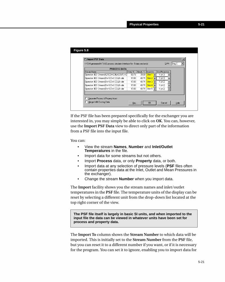
Physical Properties 5-21

If the PSF file has been prepared specifically for the exchanger you are interested in, you may simply be able to click on OK. You can, however, use the Import PSF Data view to direct only part of the information from a PSF file into the input file.

You can:

• View the stream Names, Number and Inlet/Outlet Temperatures in the file.

• Import data for some streams but not others.• Import Process data, or only Property data, or both.• Import data at any selection of pressure levels (PSF files often

contain properties data at the Inlet, Outlet and Mean Pressures in the exchanger).

• Change the stream Number when you import data.

The Import facility shows you the stream names and inlet/outlet temperatures in the PSF file. The temperature units of the display can be reset by selecting a different unit from the drop-down list located at the top right corner of the view.

The Import To column shows the Stream Number to which data will be imported. This is initially set to the Stream Number from the PSF file, but you can reset it to a different number if you want, or if it is necessary for the program. You can set it to ignore, enabling you to import data for

Figure 5.8

The PSF file itself is largely in basic SI units, and when imported to the input file the data can be viewed in whatever units have been set for process and property data.

5-21

5-22 Importing Properties and Process Data

only one stream (or fewer than all the streams for multi-stream exchangers). You cannot set two stream numbers to be the same.

The Use Properties column lets you select which pressure levels in a PSF file to use for Properties data. If there are data for three pressure levels, you can select two (upper and lower), one (middle level), or you can opt for a special selection.

If you want to import the properties data but not the process data, click on Separate Process and Properties, and you will see that the Import To column is divided in two. The left part relates to Process data, the right part to Properties. You can set either one to Ignore, so that only the other is imported.

Normally, when you import Process and/or Properties data for a stream, any data you have already entered for that stream is overwritten. You can however, cause the Properties data to be added to any data currently present, provided that it relates to a different pressure. Use the Merge with Existing Data checkbox.

Click on OK to transfer the Process/Properties data selected from the PSF file to the input file. Select Input-Process or Properties (old style) from the menu bar to see what has been imported.

PSF file layout and contents are defined in the Help Text.

5-22

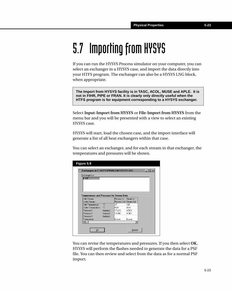
Physical Properties 5-23

5.7 Importing from HYSYSIf you can run the HYSYS Process simulator on your computer, you can select an exchanger in a HYSYS case, and import the data directly into your HTFS program. The exchanger can also be a HYSYS LNG block, when appropriate.

Select Input-Import from HYSYS or File-Import from HYSYS from the menu bar and you will be presented with a view to select an existing HYSYS case.

HYSYS will start, load the chosen case, and the import interface will generate a list of all heat exchangers within that case.

You can select an exchanger, and for each stream in that exchanger, the temperatures and pressures will be shown.

You can revise the temperatures and pressures. If you then select OK, HYSYS will perform the flashes needed to generate the data for a PSF file. You can then review and select from the data as for a normal PSF import.

The Import from HYSYS facility is in TASC, ACOL, MUSE and APLE. It is not in FIHR, PIPE or FRAN. It is clearly only directly useful when the HTFS program is for equipment corresponding to a HYSYS exchanger.

Figure 5.9

5-23

5-24 Importing from Properties Package

5.8 Importing from Properties Package

There is an option for importing properties and process data by accessing your company’s own physical properties software while you are running an HTFS program. If this facility has been made available, the Import from Other Package command under the File menu will be active.

When you select this option, you are asked to provide input on stream inlet/outlet conditions, stream compositions and components, and possibly also on the methods to be used, and the temperature/pressure range of data to be set up. When you have supplied the necessary information, a PSF file will be generated, and you will be taken to the PSF import facility, where you can opt to import the data you have created into the input file of your HTFS program.

To set up a facility to import data from your company’s own physical properties software you must write an interface to this property package and register it so that your HTFS program will recognise it. You must create an executable with project name Properties Package and a class name PSFFileGen.

The Help Text provides detailed information on the structure of the interface, and on the contents of the PSF file it must generate.

5-24

Physical Properties 5-25

5.9 Properties OutputThe Physical Properties Package can be used to generate two types of output. The first is in file format, the second in Windows format. All the output relates to tables of property values which are set up at the beginning of the program, and subsequently interpolated during heat transfer and pressure drop calculations. In addition to these two types of output, all the properties method information relating to how you set up any COMThermo properties is recorded when you save the program input file.

The first type of output can be either held in a separate file, or directed to the main Lineprinter file. The separate file is the default. If you want it in the main Lineprinter output, or turned off, select this on the Output Options view, this view can be opened by selecting Input-Options from the menu bar.

Putting the Physical Properties output in the Lineprinter file means that you will be able to see it in the Full Results output, in programs with this facility.

The contents of the file format Physical Properties output can be set via the Properties Output Options view. The Properties Output Options view is accessible from the main Physical Properties (old style) input view. The output is in four parts:

• Input data for each stream/pressure level.• Table of properties for each stream/pressure level.• Stream/phase compositions for each stream/pressure level.• Table of properties for each component.

The third and fourth items are only relevant where mixture calculations have been performed. Only the second item is produced by default. See the Help Text for more information on the contents of the various parts of the output. A further option, accessible via Output, lets you output stream data to a stream properties databank (see Section 5.5 - Property Databanks).

The second type of Physical Properties Package output, in Windows format, is not yet available in all HTFS programs. When it is available, you will see Stream Properties and T-h-x as Output menu commands.

5-25

5-26 Pressure Dependence

Stream Properties gives the properties of each phase in both tabular and graphical forms. The graphical form has a range of options. The default is to plot all properties relative to their maximum value, so you can immediately see if any property does not have a smooth variation. This can be very useful for identifying typographical errors if you have input the properties data yourself.

T-h-x gives tabular or graphical presentations of the temperature, specific enthalpy and quality (vapour mass fraction) for each stream. The graphical version also shows a set of interpolated points, so that you can see the way properties data (input or calculated) is interpreted when it is interpolated during heat transfer calculations.

5.10 Pressure DependenceThe effect of pressure on properties is most likely to be significant in the changes it produces in vapour density, and in dew and bubble points, which may be important when there is a close temperature approach between streams. Allowing for pressure dependence is optional in most HTFS programs

The normal way of ensuring pressure dependence is allowed for is to provide properties data at two pressure levels.

If you are using the program to calculate stream properties for a mixture of known composition, then it is very simple to define two pressure levels in the properties input. This normally happens by default when you are using COMThermo. If you are using Physical Properties (old style) input you will need to use the Add Pressure key. You must then specify the pressure for each level (if you only have one level, you can use a default pressure). You should select the pressures to span the range expected in the exchanger.

You can specify data at more than two pressure levels for a stream. This is unlikely to be necessary if the stream pressure change is less than 30% of the (absolute) inlet pressure.

When data are available at only one pressure, the PPP can, if specified, estimate an allowance for pressure dependence, using the Clausius Clapeyron equation. This will be less accurate for wide boiling range

5-26

Physical Properties 5-27

mixtures. To allow for pressure dependence in such cases, use the checkbox on the main Physical Properties (old style) input view.

If you are supplying pre-calculated properties data at two pressures, you should use specific enthalpies, not heat loads, and ensure that the enthalpies have a consistent zero.

If the properties data you have available are not isobaric data, but contain some inherent pressure dependence, for example from inlet to outlet, then in many cases you can use this data with relatively minor inaccuracies. You should not select Pressure Dependence in such cases. Data with an inherent pressure dependence are, however, not acceptable for two-phase streams that are pure substances, or azeotropes, or for which the change in saturation temperature due to pressure changes is comparable with, or larger than, the isobaric boiling range.

5-27

5-28 Pressure Dependence

5-28

Other Facilities 6-1

6 Other Facilities

6-1

6.1 Overview...........................................................................................3

6.2 The Setting Plan...............................................................................3

6.2.1 The Tube Layout Drawing.........................................................5

6.3 The Costing Package.......................................................................6

6.4 The Word Specification Sheet ........................................................8

6.5 The Lowfin Tube Databank .............................................................9

6.6 Project File Structure ....................................................................10

6-2 Other Facilities

6-2

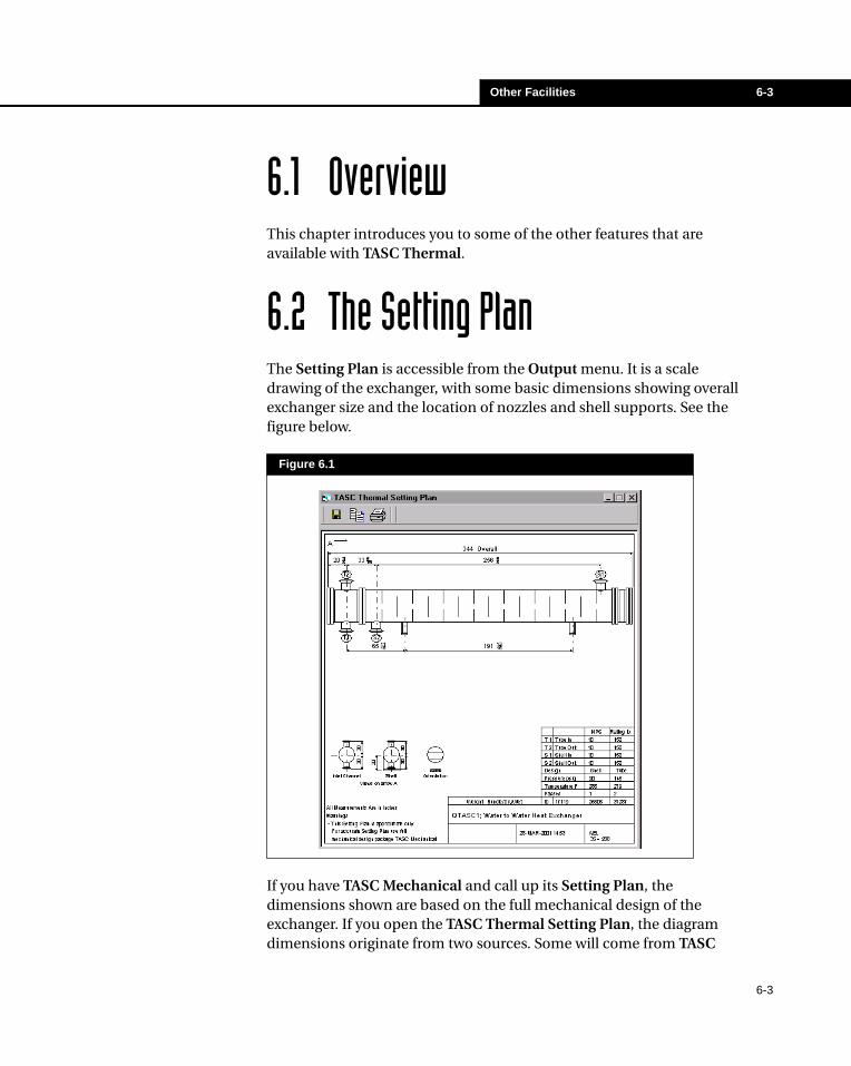
Other Facilities 6-3

6.1 OverviewThis chapter introduces you to some of the other features that are available with TASC Thermal.

6.2 The Setting PlanThe Setting Plan is accessible from the Output menu. It is a scale drawing of the exchanger, with some basic dimensions showing overall exchanger size and the location of nozzles and shell supports. See the figure below.

If you have TASC Mechanical and call up its Setting Plan, the dimensions shown are based on the full mechanical design of the exchanger. If you open the TASC Thermal Setting Plan, the diagram dimensions originate from two sources. Some will come from TASC

Figure 6.1

6-3

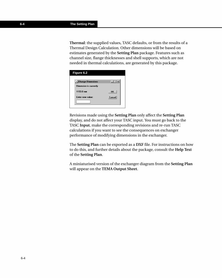
6-4 The Setting Plan

Thermal: the supplied values, TASC defaults, or from the results of a Thermal Design Calculation. Other dimensions will be based on estimates generated by the Setting Plan package. Features such as channel size, flange thicknesses and shell supports, which are not needed in thermal calculations, are generated by this package.

Revisions made using the Setting Plan only affect the Setting Plan display, and do not affect your TASC input. You must go back to the TASC Input, make the corresponding revisions and re-run TASC calculations if you want to see the consequences on exchanger performance of modifying dimensions in the exchanger.

The Setting Plan can be exported as a DXF file. For instructions on how to do this, and further details about the package, consult the Help Text of the Setting Plan.

A miniaturised version of the exchanger diagram from the Setting Plan will appear on the TEMA Output Sheet.

Figure 6.2

6-4

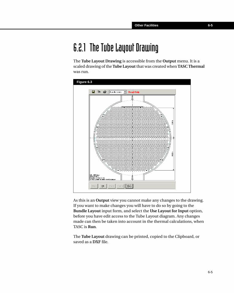
Other Facilities 6-5

6.2.1 The Tube Layout DrawingThe Tube Layout Drawing is accessible from the Output menu. It is a scaled drawing of the Tube Layout that was created when TASC Thermal was run.

As this is an Output view you cannot make any changes to the drawing. If you want to make changes you will have to do so by going to the Bundle Layout input form, and select the Use Layout for Input option, before you have edit access to the Tube Layout diagram. Any changes made can then be taken into account in the thermal calculations, when TASC is Run.

The Tube Layout drawing can be printed, copied to the Clipboard, or saved as a DXF file.

Figure 6.3

6-5

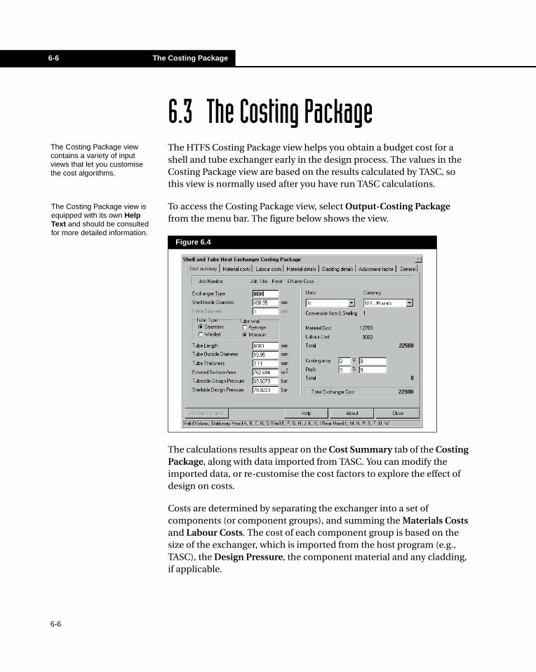
6-6 The Costing Package

6.3 The Costing PackageThe HTFS Costing Package view helps you obtain a budget cost for a shell and tube exchanger early in the design process. The values in the Costing Package view are based on the results calculated by TASC, so this view is normally used after you have run TASC calculations.

To access the Costing Package view, select Output-Costing Package from the menu bar. The figure below shows the view.

The calculations results appear on the Cost Summary tab of the Costing Package, along with data imported from TASC. You can modify the imported data, or re-customise the cost factors to explore the effect of design on costs.

Costs are determined by separating the exchanger into a set of components (or component groups), and summing the Materials Costs and Labour Costs. The cost of each component group is based on the size of the exchanger, which is imported from the host program (e.g., TASC), the Design Pressure, the component material and any cladding, if applicable.

Figure 6.4

The Costing Package view contains a variety of input views that let you customise the cost algorithms.

The Costing Package view is equipped with its own Help Text and should be consulted for more detailed information.

6-6

Other Facilities 6-7

The package contains tables of cost data for various components, based on Carbon Steel, and then cost factors are applied to allow for other materials. You can change these cost factors to allow for current market conditions. Add other Adjustment Factors for each component group to customise the costs for your company, and to allow for inflation. These customisation factors may be saved to a file for future use, and should be periodically adjusted to reflect changing costs.

Exchanger costs are, of course, sensitive to Materials Costs and market conditions, and will differ between regions and countries. Using the package in its basic form will only give a very approximate budget cost. If you customise the package you can improve its relevance to your company. Even if you do not customise it, the Costing Package can be useful in showing the relative costs of two possible designs.

Methods in the Costing Package are different from the much simpler relative cost algorithms used to compare designs in the core TASC program, and are not intended to replace them.

6-7

6-8 The Word Specification Sheet

6.4 The Word Specification SheetThe Word Specification Sheet can be used if you have Microsoft® Word for Windows (Word 6 or higher). The Word Template (TEMAWW60.DOT) supplied has a standard TEMA type layout, equivalent to what you see in the TASC internal TEMA Input/Output sheet.

Before using the Word Specification Sheet you must specify the location of the relevant WINWORD.EXE file in your TASC Preferences. In the Preferences view, go to the tab marked Word and specify the path of the WINWORD.EXE file of the version of Word you are using in the Word Processor group. You can also select the Template file (extension *.DOT) to be used by specifying the path in the Tema Sheet Template group.

After running TASC calculations, open the Word Specification Sheet by selecting Output-Word Spec Sheet from the menu bar. The Word template is opened, which you can edit and/or save as a *.DOC, specifying the file name and location.

You can edit the template to contain information relevant to your company. It can be translated into a different language, if required. If you do so, it is a good idea to save the new template with a different name, keeping the original template on file. You can create multiple templates, and select from among them when you run TASC. Use the Word tab in the Preferences view to set the template to be used.

The templates contain Bookmarks. TASC uses OLE automation transfer data calculated and/or held within the TASC User Interface to the Word file. The Bookmarks can be re-arranged or deleted. You cannot modify them or add new ones. See your Word manual for more information.

To access the Preferences view, select File-Preferences from the menu bar.

To access the Preferences view, select File-Preferences from the menu bar.

6-8

Other Facilities 6-9

6.5 The Lowfin Tube DatabankTo specify a Lowfin Tube in the input data:

1. Open the Bundle Geometry property view.

2. On the Tube Details tab, set the Tube Type to Lowfin Tubes and specify the tube outside diameter and (minimum) wall thickness.

3. Open the Enhanced Surfaces property view by selecting Input-Enhanced Surfaces from the menu bar.

4. Click on the Lowfin Tube (as input or from bank) drop-down list.

You will see a list of the fins in the Lowfin databank. This is in the form of a code, identifying the fins per inch, fin thickness and fin height. See the Help Text for more information.

The Lowfin data bank is a text file, LOWFIN.TXT, which is supplied with TASC. You can make additions to the bank, using the same format as the included items. The first item in the bank as supplied has explanatory text at the side. Each fin requires a unique identification number, in the range 2001 to 2999. Identify the fins per inch, together with the fin pitch, height and thickness. You should then identify the tube diameters for which the fin is available and the range of wall thicknesses for each tube, if possible. Any such data should come from a tube manufacturer.

6-9

6-10 Project File Structure

6.6 Project File StructureA TASC Project is initially set up as an input file. The various files are outlined in the following table.

When you Run calculations from the User Interface, most of the project output files are set up by default. You are able to switch off some of the files by using the features available in the Options view.

1. Access the Options view by selecting Input-Options from the menu bar.

2. On the Options view, go to the Output Options tab.

3. The Output Options tab contains drop-down lists controlling these outputs.

The file extension *.TAA is used for an edited copy of the input data. This is the version stored internally by the User Interface, which you can run without saving. If you save the file, the main input, name.TAI is updated. The *.TAA file is not saved when TASC is shut down.

File Name Description

name.TAI Where name is the name of the Project. After you have run the project, some or all the following files will also have been set up.

name.TAF The so-called Intout file, containing all the main input and results. The format of this file is described in Intout.doc in the \TOOLS\TASC\INTOUT Directory on the HTFS Software CD. All the TASC Results views, which you can view under Output, take data from this file. You can use this file as a source of information for in-house software.

name.TAL The Lineprinter output file.

name.TAT The 80-column output file.

name.TAE The Error/Warning Messages file.

name.TAV The Brief Summary output file.

name.TAP The Physical Properties output file.

You cannot switch off the *.TAF file, which is needed for the main Output views, or the Error/Warning log.

6-10

Examples 7-1

7 Examples

7-1

7.1 Overview...........................................................................................3

7.2 High Pressure Boiler Feedwater Heater ........................................4

7.2.1 Start Up View ...........................................................................57.2.2 Entering the Data .....................................................................67.2.3 Running the TASC Calculations .............................................117.2.4 Examining the Results............................................................127.2.5 What next? .............................................................................15

7.3 Debutanizer Overhead Condenser...............................................16

7.3.1 Enter the Data ........................................................................177.3.2 Run TASC Thermal ................................................................217.3.3 Examining the Results............................................................22

7.4 Kettle Reboiler ...............................................................................23

7.4.1 Enter the Data ........................................................................257.4.2 Examining the Results............................................................29

7.5 Falling Film Evaporator .................................................................31

7.5.1 Enter the data.........................................................................337.5.2 Examining the Results............................................................35

7.6 Feed Effluent Train ........................................................................37

7.6.1 Examining the Results............................................................42

7.7 Vertical Thermosyphon Reboiler .................................................45

7.7.1 Enter the Data ........................................................................487.7.2 Examining the Results............................................................53

7.8 Horizontal Thermosyphon Reboiler.............................................54

7-2 Examples

7-2

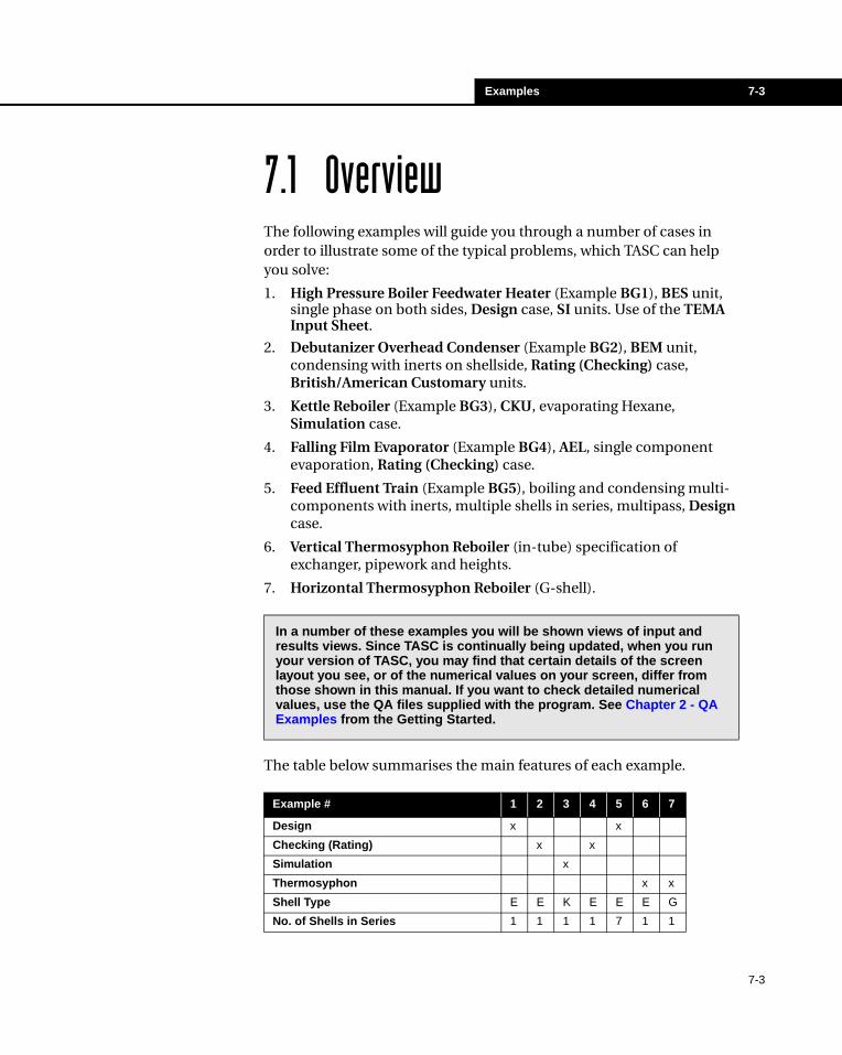
Examples 7-3

7.1 OverviewThe following examples will guide you through a number of cases in order to illustrate some of the typical problems, which TASC can help you solve:

1. High Pressure Boiler Feedwater Heater (Example BG1), BES unit, single phase on both sides, Design case, SI units. Use of the TEMA Input Sheet.

2. Debutanizer Overhead Condenser (Example BG2), BEM unit, condensing with inerts on shellside, Rating (Checking) case, British/American Customary units.

3. Kettle Reboiler (Example BG3), CKU, evaporating Hexane, Simulation case.

4. Falling Film Evaporator (Example BG4), AEL, single component evaporation, Rating (Checking) case.

5. Feed Effluent Train (Example BG5), boiling and condensing multi-components with inerts, multiple shells in series, multipass, Design case.

6. Vertical Thermosyphon Reboiler (in-tube) specification of exchanger, pipework and heights.

7. Horizontal Thermosyphon Reboiler (G-shell).

The table below summarises the main features of each example.

In a number of these examples you will be shown views of input and results views. Since TASC is continually being updated, when you run your version of TASC, you may find that certain details of the screen layout you see, or of the numerical values on your screen, differ from those shown in this manual. If you want to check detailed numerical values, use the QA files supplied with the program. See Chapter 2 - QA Examples from the Getting Started.

Example # 1 2 3 4 5 6 7

Design x x

Checking (Rating) x x

Simulation x

Thermosyphon x x

Shell Type E E K E E E G

No. of Shells in Series 1 1 1 1 7 1 1

7-3

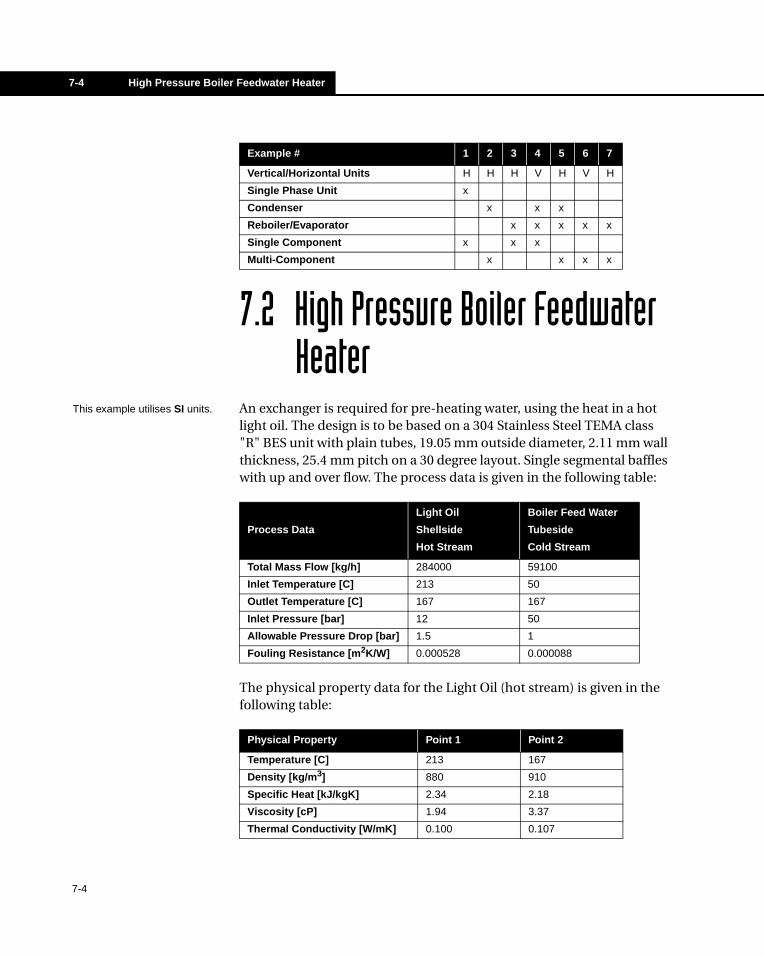
7-4 High Pressure Boiler Feedwater Heater

7.2 High Pressure Boiler Feedwater Heater

An exchanger is required for pre-heating water, using the heat in a hot light oil. The design is to be based on a 304 Stainless Steel TEMA class "R" BES unit with plain tubes, 19.05 mm outside diameter, 2.11 mm wall thickness, 25.4 mm pitch on a 30 degree layout. Single segmental baffles with up and over flow. The process data is given in the following table:

The physical property data for the Light Oil (hot stream) is given in the following table:

Vertical/Horizontal Units H H H V H V H

Single Phase Unit x

Condenser x x x

Reboiler/Evaporator x x x x x

Single Component x x x

Multi-Component x x x x

Process Data

Light Oil

Shellside

Hot Stream

Boiler Feed Water

Tubeside

Cold Stream

Total Mass Flow [kg/h] 284000 59100

Inlet Temperature [C] 213 50

Outlet Temperature [C] 167 167

Inlet Pressure [bar] 12 50

Allowable Pressure Drop [bar] 1.5 1

Fouling Resistance [m2K/W] 0.000528 0.000088

Physical Property Point 1 Point 2

Temperature [C] 213 167

Density [kg/m3] 880 910

Specific Heat [kJ/kgK] 2.34 2.18

Viscosity [cP] 1.94 3.37

Thermal Conductivity [W/mK] 0.100 0.107

Example # 1 2 3 4 5 6 7

This example utilises SI units.

7-4

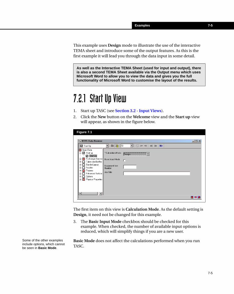
Examples 7-5

This example uses Design mode to illustrate the use of the interactive TEMA sheet and introduce some of the output features. As this is the first example it will lead you through the data input in some detail.

7.2.1 Start Up View1. Start up TASC (see Section 3.2 - Input Views).

2. Click the New button on the Welcome view and the Start up view will appear, as shown in the figure below.

The first item on this view is Calculation Mode. As the default setting is Design, it need not be changed for this example.

3. The Basic Input Mode checkbox should be checked for this example. When checked, the number of available input options is reduced, which will simplify things if you are a new user.

Basic Mode does not affect the calculations performed when you run TASC.

As well as the Interactive TEMA Sheet (used for input and output), there is also a second TEMA Sheet available via the Output menu which uses Microsoft Word to allow you to view the data and gives you the full functionality of Microsoft Word to customise the layout of the results.

Figure 7.1

Some of the other examples include options, which cannot be seen in Basic Mode.

7-5

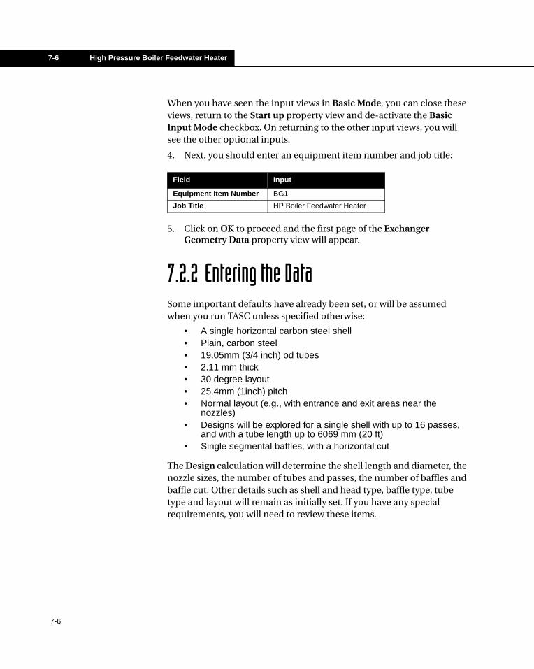
7-6 High Pressure Boiler Feedwater Heater

When you have seen the input views in Basic Mode, you can close these views, return to the Start up property view and de-activate the Basic Input Mode checkbox. On returning to the other input views, you will see the other optional inputs.

4. Next, you should enter an equipment item number and job title:

5. Click on OK to proceed and the first page of the Exchanger Geometry Data property view will appear.

7.2.2 Entering the DataSome important defaults have already been set, or will be assumed when you run TASC unless specified otherwise:

• A single horizontal carbon steel shell• Plain, carbon steel• 19.05mm (3/4 inch) od tubes• 2.11 mm thick• 30 degree layout• 25.4mm (1inch) pitch• Normal layout (e.g., with entrance and exit areas near the

nozzles)• Designs will be explored for a single shell with up to 16 passes,

and with a tube length up to 6069 mm (20 ft)• Single segmental baffles, with a horizontal cut

The Design calculation will determine the shell length and diameter, the nozzle sizes, the number of tubes and passes, the number of baffles and baffle cut. Other details such as shell and head type, baffle type, tube type and layout will remain as initially set. If you have any special requirements, you will need to review these items.

Field Input

Equipment Item Number BG1

Job Title HP Boiler Feedwater Heater

7-6

Examples 7-7

Some items still need to be set. You will see that Side for the Hot Stream is Not Yet Set so you must specify the hot side.

1. Define the fields in the Exchanger Geometry view as detailed in the following table:

All other information can be left at their default settings.

2. Click on OK to save the data and close the form.

As an alternative to using the standard input views, there is an interactive TEMA input sheet that for simple cases will allow you to enter the data and see the results.

3. Select Input-TEMA Input from the menu bar. See Figure 7.2 for a view of the TEMA sheet.

For this example, the input units should be set to SI. If you want to change from Metric or British/American Customary then select Units from the menu options at the top of the TEMA Specification Sheet and click on the unit set with which you want to work.

In order to make the sheet easier to read you can use the functions in the View menu to enlarge or zoom into areas of the sheet.

Data can be entered on the TEMA Sheet in any of the areas marked light blue (this is the default colour - if you have changed your Windows colour scheme it may be different). The data in this sheet are linked to the normal data input property views in TASC, and vice versa, so either method of input can be used at any time (the next example illustrates the use of the main input property views). As you move the cursor around the sheet you will find in some cases drop-down lists become available. You may also enter data in grey fields but these data are not necessary for a run of TASC - they are treated simply as comments.

Field Input

Front End Head Type TEMA B

Rear End Head Type TEMA S

Side for Hot Stream Shell-side Hot

The SI, British/American and Metric units of input and output used by HTFS are not the pure units but a more convenient set (e.g., SI flowrate in kg/h not kg/s, SI/Metric length in mm not m, viscosity in cP for all sets of units).

If you have a case where the stream allocation is not clear, TASC makes it easy to try both in Design mode. You simply change the Side for Hot Stream setting and re-run.

Units are always the same across a case(i.e., length is always mm or inches whether for tube diameter or tube length).

Help may be obtained at any time by placing the cursor on an item and pressing F1.

7-7

7-8 High Pressure Boiler Feedwater Heater

You now need to enter the remaining data for this case.

4. Look at the TEMA Type on line 6. If you have not already set B E S, you can click on these items (there are three separate drop-down lists) to set them.

5. For the shellside (hot oil) enter the following information.

6. For the tubeside (water) enter the following information.

Field Input

Fluid Name Hot Oil

Fluid Quantity [kg/h] 284000

Temperature In [C] 213

Temperature Out [C] 167

Inlet Pressure [bar abs] 12

Allowable Pressure Drop [bar] 1.5

Fouling Resistance [m2K/W] 0.000528

Field Input

Fluid Name Boiler Water Feed

Fluid Quantity - Total [kg/h] 59100

Temperature In [C] 50

Temperature Out [C] 167

Inlet Pressure [bar abs] 50

Allowable Pressure Drop [bar] 1.0

Fouling Resistance [m2K/W] 0.000088

The Allowable Pressure Drop for both the shellside and tubeside streams will change to the calculated pressure drop once TASC has performed its calculations.

The Fouling Resistance of the tubeside stream will change when TASC has calculated the results, since all output coefficients relate to the tube outside diameter.

7-8

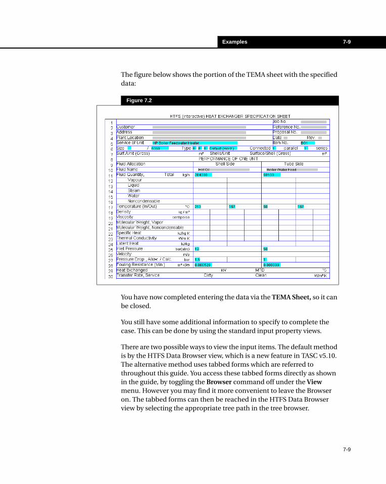
Examples 7-9

The figure below shows the portion of the TEMA sheet with the specified data:

You have now completed entering the data via the TEMA Sheet, so it can be closed.

You still have some additional information to specify to complete the case. This can be done by using the standard input property views.

There are two possible ways to view the input items. The default method is by the HTFS Data Browser view, which is a new feature in TASC v5.10. The alternative method uses tabbed forms which are referred to throughout this guide. You access these tabbed forms directly as shown in the guide, by toggling the Browser command off under the View menu. However you may find it more convenient to leave the Browser on. The tabbed forms can then be reached in the HTFS Data Browser view by selecting the appropriate tree path in the tree browser.

Figure 7.2

7-9

7-10 High Pressure Boiler Feedwater Heater

7. From the main menu bar select Input-Exchanger Geometry. This provides a property view with two tabs.

8. Specify as a material 304 Stainless Steel (the default would be Carbon Steel). Click on the Material Properties tab and select 304 Stainless from the Tube Material drop-down list.

9. Click OK to save the data and close the form

You must now specify the physical properties of the fluids.

10. Select Input-Physical Properties from the main menu bar. You will see a form with two tabs, one for the Hot Stream and the other for the Cold Stream.

11. Select Direct Input as the stream data source.

12. On the Hot Stream tab enter the property data as shown in the table below.

With the HTFS Data Browser, the Apply and OK buttons are no longer necessary. These both occur automatically when you move from one page/input form to another, or in general when you leave a page/input form.

On each property view, input data is accepted by moving to another tab, by clicking on Apply or on OK (which also closes the form), or by closing the form. If you click Cancel, it will lose any newly entered data on the currently visible tab, and close that property view.

Physical properties can also be entered via the Physical Properties (Old Style) input views.

Physical Property Point 1 Point 2

Temperature [C] 213 167

Density [kg/m3] 880 910

Specific Heat [kJ/kgK] 2.34 2.18

Viscosity [cP] 1.94 3.37

Thermal Conductivity [W/mK] 0.100 0.107

These values are associated with pressure level 1. As there is no data for pressure level 2 delete the pressure from the pressure level table.

When not in Basic Input Mode, the Exchanger Geometry property view consists of four tabs.

The hot key SHIFT F12 will also open the Physical Property Data view.

7-10

Examples 7-11

13. Select the Cold Stream tab.

14. Select Water (NEL40) as the stream data source.

15. Close the form.

You have now entered all the data and should save this in case you want to use it again in the future.

16. From the main menu bar, select File-Save (or Save As). This will then present a standard Windows File form.

17. Change the directory if you want and then change the default name to BG1.TAI and click OK.

7.2.3 Running the TASC Calculations1. From the main menu bar select Run-Calculate All.

TASC will check the data supplied for consistency, correct any minor errors where possible and start the Design calculation. It will show where it has reached at any time within the run view that appears.

2. On completion, the Summary view will automatically open. If there have been any problems an Error/Message Log view will also appear.

The TASC Design logic will attempt to optimise the heat transfer against the allowable pressure drop on both the shell and tube sides. It also has built in heuristic rules that will stop it searching once it realises that further calculations are pointless. As a general rule TASC will attempt to design small diameter single pass exchangers before increasing the tube length, shell diameter, number of passes and number of shells.

You only need to input BG1 when saving your case. The extension.TAI is always used for TASC input files, and is added automatically.

Pressing F4 will also initiate the TASC calculations.

7-11

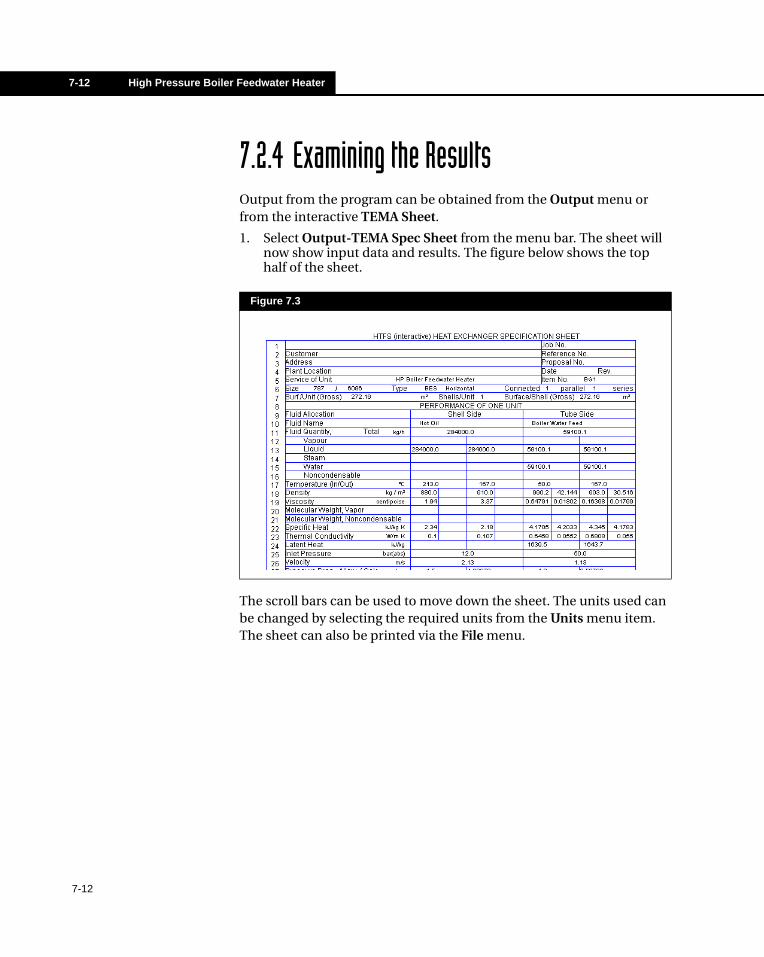
7-12 High Pressure Boiler Feedwater Heater

7.2.4 Examining the ResultsOutput from the program can be obtained from the Output menu or from the interactive TEMA Sheet.

1. Select Output-TEMA Spec Sheet from the menu bar. The sheet will now show input data and results. The figure below shows the top half of the sheet.

The scroll bars can be used to move down the sheet. The units used can be changed by selecting the required units from the Units menu item. The sheet can also be printed via the File menu.

Figure 7.3

7-12

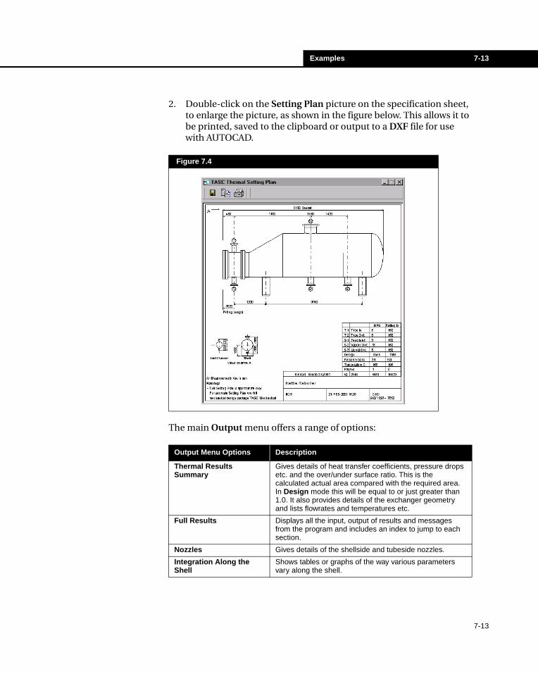
Examples 7-13

2. Double-click on the Setting Plan picture on the specification sheet, to enlarge the picture, as shown in the figure below. This allows it to be printed, saved to the clipboard or output to a DXF file for use with AUTOCAD.

The main Output menu offers a range of options:

Figure 7.4

Output Menu Options Description

Thermal Results Summary

Gives details of heat transfer coefficients, pressure drops etc. and the over/under surface ratio. This is the calculated actual area compared with the required area. In Design mode this will be equal to or just greater than 1.0. It also provides details of the exchanger geometry and lists flowrates and temperatures etc.

Full Results Displays all the input, output of results and messages from the program and includes an index to jump to each section.

Nozzles Gives details of the shellside and tubeside nozzles.

Integration Along the Shell

Shows tables or graphs of the way various parameters vary along the shell.

7-13

7-14 High Pressure Boiler Feedwater Heater

Alternative Designs Only available in Design mode and provides a list of all the designs found that achieve the duty. You will see that one column gives the cost ratio of the various designs to the lowest cost design which TASC has selected, and which was shown in the summary table.

Word Spec Sheet Automatically starts Microsoft Word for Windows, with a document based on a template of a TEMA Specification Sheet. It automatically loads the data (input and results) from the current run of TASC. The advantage that this has over the interactive TEMA Sheet is that this sheet, or its template, can be customised to your own preferences. You can also paste into it from the clipboard the setting plan, graphs, tube layout etc. and then save it as a document for the exchanger you are considering. If you do customise the template of the sheet to add extra pages, logos etc. then you should save it under a new name in the same directory as TASC. You can then select to use this new customised template via File- Preferences from the main menu bar.

TEMA Spec Sheet Views the interactive TEMA Sheet. This is the sheet used earlier to provide some of the input data, but it now has all the calculated results filled in.

Setting Plan Provides a scale drawing of the exchanger which is intended to give an indication of the position of nozzles and supports and the approximate weight of the exchanger. See Figure 7.4. TASC performs a simplified mechanical calculation in order to obtain the sizes. Where possible this calculation uses properties of the exchanger material you have specified, but for simplicity, certain aspects are based on typical values for a carbon steel exchanger. Care is thus needed if other materials are used. TASC Mechanical can perform a full mechanical design calculation and so will supply accurate dimensions when it is used in conjunction with the Setting Plan.

Costing Package Allows you to undertake a budget costing of the exchanger. The prices of materials and labour etc. can be customised and saved for re-use.

Report Generator Provides printing and export of selected output tables and graphs, and the Setting Plan.

Tube Layout Not available in Design Mode.

Brief Output Single page summary file of all the main results.

Bill of Materials Refer to TASC Mechanical.

Print Calculations Refer to TASC Mechanical.

Sketch Refer to TASC Mechanical.

Stream Properties Shows tables or graphs of property as input.

T-h-x Shows tables or graphs of the variation of enthalpy and quality with temperature.

Lineprinter Contains all the input, output of results and messages from the program.

Output Menu Options Description

TASC uses a very simple costing algorithm in Design in order to undertake cost comparisons - it is not the same method as used for budget costing which can be selected via the Output menu.

You should look at the other designs, and if there are some that have a cost ratio only a small amount above unity, consider whether they have other features, which make them more attractive than the chosen design.

7-14

Examples 7-15

7.2.5 What next?The Design mode of TASC will provide a number of designs that will achieve the required duty. However, you will probably want to fine tune and fully optimise the design. This is best achieved via Rating (Checking) mode.

1. Select File-Create Checking Case from the main menu bar. This will then prompt you for the name of a data file, which will be used to save the Checking data - enter BG1C.TAI. You will then be shown a table of possible designs presented in a spreadsheet type form. A row headed Cost Item/Chosen, shows ratios of the costs of alternative designs to the cheapest design. The design with the ratio of 1 is the design for which TASC has shown full details.

2. To select the design you want to look at in more detail, click on the Design Number located at the top of the table. The table of alternative designs will now close, the Process Diagram will be displayed and it will show Checking Case.

You can now "fine tune" the design by considering whether the baffle pitch, end lengths or any other features may need adjusting. This can be done via the Interactive TEMA Sheet or via individual property views from the Input menu.

80 Column Old file format that fits in 80 columns and contains both input and results but it is not so comprehensive as the line printer file.

Physical Property A detailed output of the physical properties used within the program. If required, you can specify via the Input Options that you want this to be incorporated into the main lineprinter output rather than produced as a separate file.

Error Log Lists warnings and fatal errors found by the program. This information can also be found in the lineprinter output.

Output Menu Options Description

7-15

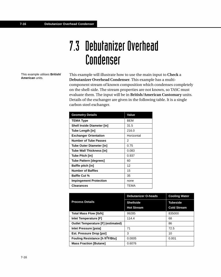
7-16 Debutanizer Overhead Condenser

7.3 Debutanizer Overhead Condenser

This example will illustrate how to use the main input to Check a Debutanizer Overhead Condenser. This example has a multi-component stream of known composition which condenses completely on the shell-side. The stream properties are not known, so TASC must evaluate them. The input will be in British/American Customary units. Details of the exchanger are given in the following table. It is a single carbon steel exchanger.

Geometry Details Value

TEMA Type BEM

Shell Inside Diameter [in] 31.5

Tube Length [in] 216.0

Exchanger Orientation Horizontal

Number of Tube Passes 2

Tube Outer Diameter [in] 0.75

Tube Wall Thickness [in] 0.083

Tube Pitch [in] 0.937

Tube Pattern [degrees] 60

Baffle pitch [in] 12

Number of Baffles 15

Baffle Cut % 35

Impingement Protection none

Clearances TEMA

Process Details

Debutanizer O-heads Cooling Water

Shellside

Hot Stream

Tubeside

Cold Stream

Total Mass Flow [lb/h] 99285 835000

Inlet Temperature [F] 114.4 68

Outlet Temperature [F] (estimated) 86

Inlet Pressure [psia] 71 72.5

Est. Pressure Drop [psi] 3 10

Fouling Resistance [h ft2F/Btu] 0.0005 0.001

Mass Fraction [Butane] 0.6076

This example utilises British/American units.

7-16

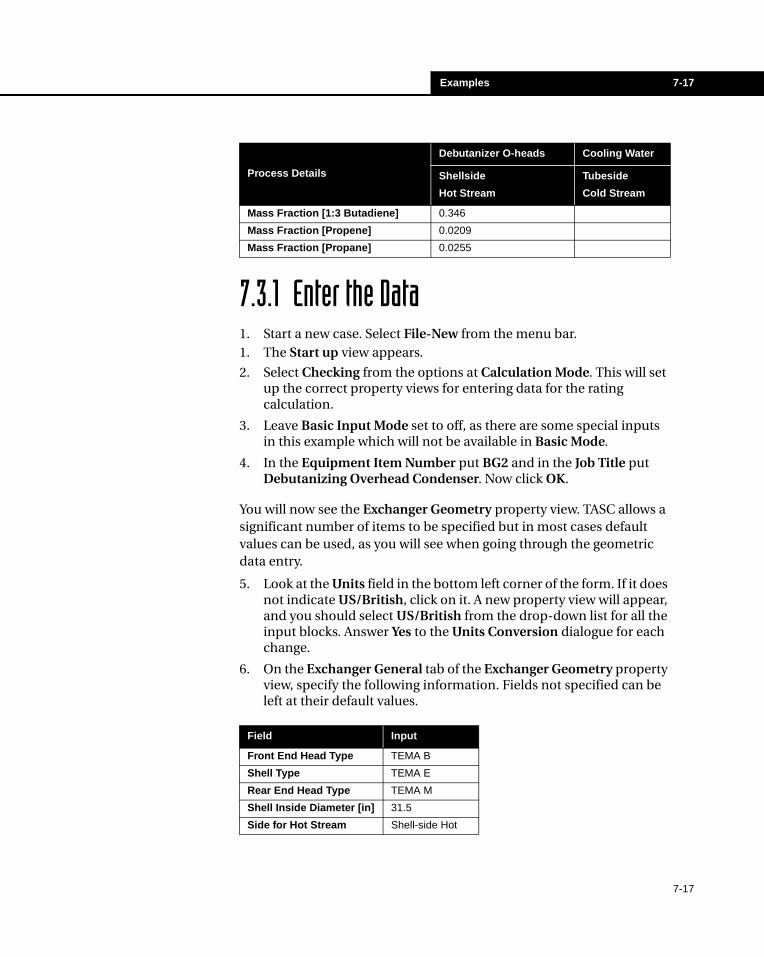
Examples 7-17

7.3.1 Enter the Data1. Start a new case. Select File-New from the menu bar.1. The Start up view appears.

2. Select Checking from the options at Calculation Mode. This will set up the correct property views for entering data for the rating calculation.

3. Leave Basic Input Mode set to off, as there are some special inputs in this example which will not be available in Basic Mode.

4. In the Equipment Item Number put BG2 and in the Job Title put Debutanizing Overhead Condenser. Now click OK.

You will now see the Exchanger Geometry property view. TASC allows a significant number of items to be specified but in most cases default values can be used, as you will see when going through the geometric data entry.

5. Look at the Units field in the bottom left corner of the form. If it does not indicate US/British, click on it. A new property view will appear, and you should select US/British from the drop-down list for all the input blocks. Answer Yes to the Units Conversion dialogue for each change.

6. On the Exchanger General tab of the Exchanger Geometry property view, specify the following information. Fields not specified can be left at their default values.

Mass Fraction [1:3 Butadiene] 0.346

Mass Fraction [Propene] 0.0209

Mass Fraction [Propane] 0.0255

Field Input

Front End Head Type TEMA B

Shell Type TEMA E

Rear End Head Type TEMA M

Shell Inside Diameter [in] 31.5

Side for Hot Stream Shell-side Hot

Process Details

Debutanizer O-heads Cooling Water

Shellside

Hot Stream

Tubeside

Cold Stream

7-17

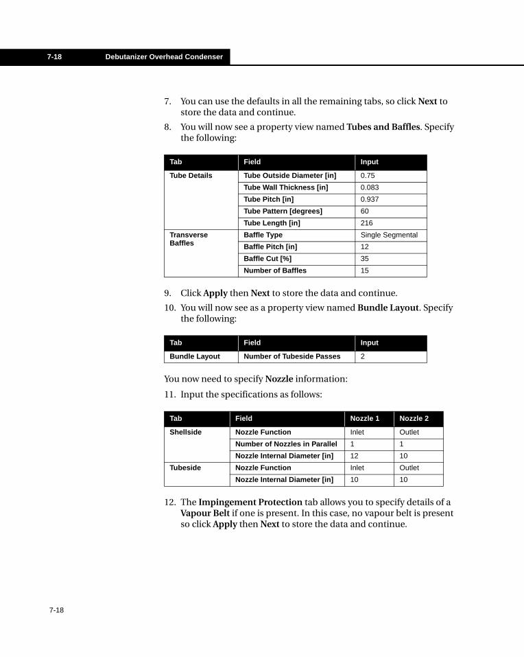
7-18 Debutanizer Overhead Condenser

7. You can use the defaults in all the remaining tabs, so click Next to store the data and continue.

8. You will now see a property view named Tubes and Baffles. Specify the following:

9. Click Apply then Next to store the data and continue.

10. You will now see as a property view named Bundle Layout. Specify the following:

You now need to specify Nozzle information:

11. Input the specifications as follows:

12. The Impingement Protection tab allows you to specify details of a Vapour Belt if one is present. In this case, no vapour belt is present so click Apply then Next to store the data and continue.

Tab Field Input

Tube Details Tube Outside Diameter [in] 0.75

Tube Wall Thickness [in] 0.083

Tube Pitch [in] 0.937

Tube Pattern [degrees] 60

Tube Length [in] 216

Transverse Baffles

Baffle Type Single Segmental

Baffle Pitch [in] 12

Baffle Cut [%] 35

Number of Baffles 15

Tab Field Input

Bundle Layout Number of Tubeside Passes 2

Tab Field Nozzle 1 Nozzle 2

Shellside Nozzle Function Inlet Outlet

Number of Nozzles in Parallel 1 1

Nozzle Internal Diameter [in] 12 10

Tubeside Nozzle Function Inlet Outlet

Nozzle Internal Diameter [in] 10 10

7-18

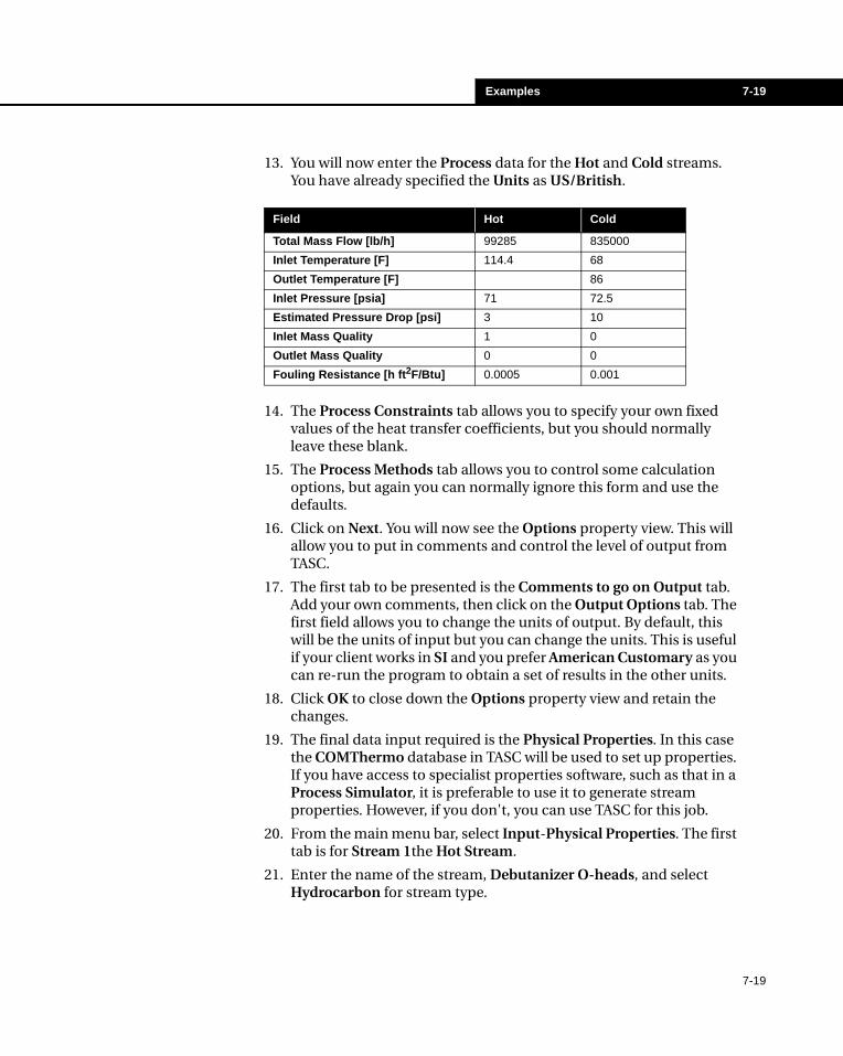
Examples 7-19

13. You will now enter the Process data for the Hot and Cold streams. You have already specified the Units as US/British.

14. The Process Constraints tab allows you to specify your own fixed values of the heat transfer coefficients, but you should normally leave these blank.

15. The Process Methods tab allows you to control some calculation options, but again you can normally ignore this form and use the defaults.

16. Click on Next. You will now see the Options property view. This will allow you to put in comments and control the level of output from TASC.

17. The first tab to be presented is the Comments to go on Output tab. Add your own comments, then click on the Output Options tab. The first field allows you to change the units of output. By default, this will be the units of input but you can change the units. This is useful if your client works in SI and you prefer American Customary as you can re-run the program to obtain a set of results in the other units.

18. Click OK to close down the Options property view and retain the changes.

19. The final data input required is the Physical Properties. In this case the COMThermo database in TASC will be used to set up properties. If you have access to specialist properties software, such as that in a Process Simulator, it is preferable to use it to generate stream properties. However, if you don't, you can use TASC for this job.

20. From the main menu bar, select Input-Physical Properties. The first tab is for Stream 1the Hot Stream.

21. Enter the name of the stream, Debutanizer O-heads, and select Hydrocarbon for stream type.

Field Hot Cold

Total Mass Flow [lb/h] 99285 835000

Inlet Temperature [F] 114.4 68

Outlet Temperature [F] 86

Inlet Pressure [psia] 71 72.5

Estimated Pressure Drop [psi] 3 10

Inlet Mass Quality 1 0

Outlet Mass Quality 0 0

Fouling Resistance [h ft2F/Btu] 0.0005 0.001

7-19

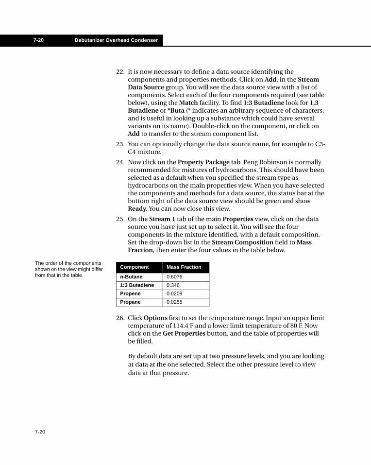
7-20 Debutanizer Overhead Condenser

22. It is now necessary to define a data source identifying the components and properties methods. Click on Add, in the Stream Data Source group. You will see the data source view with a list of components. Select each of the four components required (see table below), using the Match facility. To find 1:3 Butadiene look for 1,3 Butadiene or *Buta (* indicates an arbitrary sequence of characters, and is useful in looking up a substance which could have several variants on its name). Double-click on the component, or click on Add to transfer to the stream component list.

23. You can optionally change the data source name, for example to C3-C4 mixture.

24. Now click on the Property Package tab. Peng Robinson is normally recommended for mixtures of hydrocarbons. This should have been selected as a default when you specified the stream type as hydrocarbons on the main properties view. When you have selected the components and methods for a data source, the status bar at the bottom right of the data source view should be green and show Ready. You can now close this view.

25. On the Stream 1 tab of the main Properties view, click on the data source you have just set up to select it. You will see the four components in the mixture identified, with a default composition. Set the drop-down list in the Stream Composition field to Mass Fraction, then enter the four values in the table below.

26. Click Options first to set the temperature range. Input an upper limit temperature of 114.4 F and a lower limit temperature of 80 F. Now click on the Get Properties button, and the table of properties will be filled.

By default data are set up at two pressure levels, and you are looking at data at the one selected. Select the other pressure level to view data at that pressure.

Component Mass Fraction

n-Butane 0.6076

1:3 Butadiene 0.346

Propene 0.0209

Propane 0.0255

The order of the components shown on the view might differ from that in the table.

7-20

Examples 7-21

27. Now select Stream 2, the cold stream. Rename the stream to Cooling Water, and select data source Water from NEL40. Water data will be set up and used when the program is run, so you can now close the Properties view.

This now completes the data input for this case and the data should be saved.

28. From the main menu bar, select File-Save As.

29. On the Save As view, enter BG2 and OK to close the form.

7.3.2 Run TASC Thermal1. From the main menu bar select Run-Calculate All, or click on the

Run icon.

2. When the Tube Layout diagram appears, click on OK again.

If an inlet pressure and inlet & outlet temperatures have been input into the process input view then these will be used as defaults within the properties input. You can change the pressure levels by editing the values shown. You can change the temperatures used by using the Options button. You can either specify a range of temperatures, and leave the remainder to be set by default, or you can select Define Temperatures on Spreadsheet. This will colour the temperature line yellow, and let you edit any existing temperatures, or add ones or your own. The order in which you define them does not matter, as they are sorted whenever new data are calculated. Dew and/or bubble points are added if they are in or close to the selected temperature range.

Run icon

7-21

7-22 Debutanizer Overhead Condenser

7.3.3 Examining the ResultsOn completion of a run, TASC will automatically display the Summary view to provide an overview of the results. In this case TASC estimates that the unit is just oversized (i.e., the Actual/Required Area Ratio is greater than one).

Most of the other output options referred to in Section 7.2 - High Pressure Boiler Feedwater Heater, can also be examined in the same way as before. However, for Rating (Checking) and Simulation runs, the list of alternative designs is replaced by output of detailed information along the shell (Integration Along the Shell). The corresponding information printed in the Lineprinter File is as follows:

• Heat transfer coefficients, zone heat loads and temperatures tabulated against distance along shell (temperatures are usually printed for each tube pass, up to 4 passes and averaged if over 4 passes).

• Temperature profiles (shellside bulk, shellside fouling layer surface, shellside tube surface, tubeside tube surface, tubeside fouling layer surface and tubeside bulk temperatures) from the shellside to the tubeside tabulated against distance along shell.

This information is also available as an output view in the form of either a graph or table. If you select Output, Integration Along Shell you will then be asked which item(s) should be plotted on the Y-axis and which on the X-axis. Simply click the checkbox to select an item. Obviously more than one item can be selected for the Y-axis, but only one may be selected for the X-axis. If you choose to represent the data as a table, all values are tabulated against the axial distance.

7-22

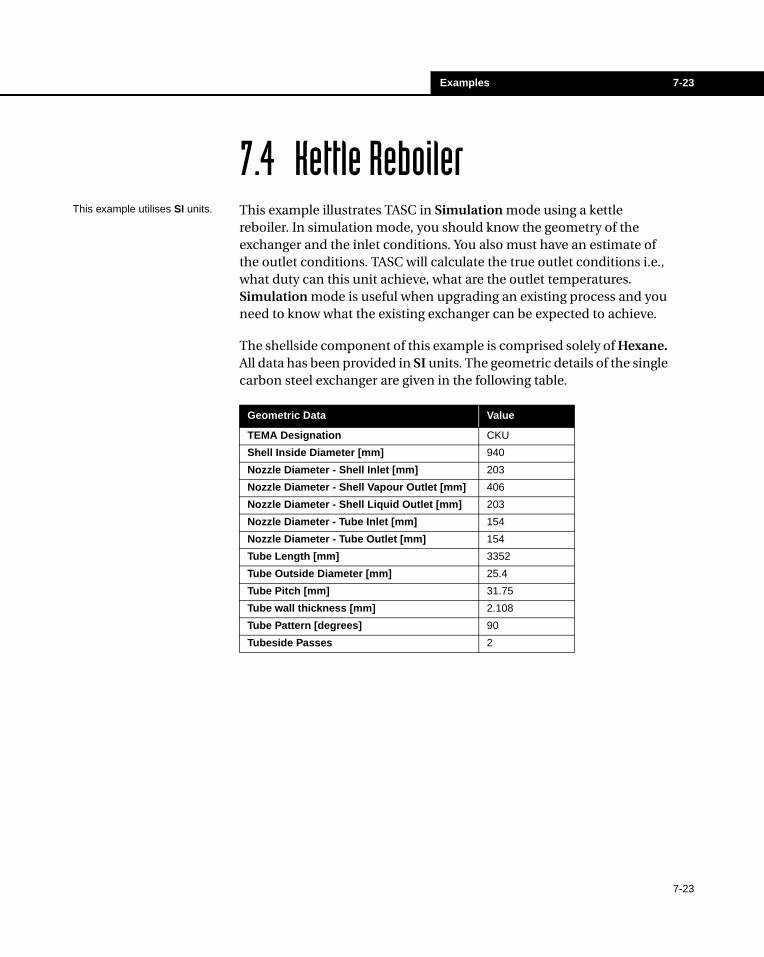
Examples 7-23

7.4 Kettle ReboilerThis example illustrates TASC in Simulation mode using a kettle reboiler. In simulation mode, you should know the geometry of the exchanger and the inlet conditions. You also must have an estimate of the outlet conditions. TASC will calculate the true outlet conditions i.e., what duty can this unit achieve, what are the outlet temperatures. Simulation mode is useful when upgrading an existing process and you need to know what the existing exchanger can be expected to achieve.

The shellside component of this example is comprised solely of Hexane. All data has been provided in SI units. The geometric details of the single carbon steel exchanger are given in the following table.

Geometric Data Value

TEMA Designation CKU

Shell Inside Diameter [mm] 940

Nozzle Diameter - Shell Inlet [mm] 203

Nozzle Diameter - Shell Vapour Outlet [mm] 406

Nozzle Diameter - Shell Liquid Outlet [mm] 203

Nozzle Diameter - Tube Inlet [mm] 154

Nozzle Diameter - Tube Outlet [mm] 154

Tube Length [mm] 3352

Tube Outside Diameter [mm] 25.4

Tube Pitch [mm] 31.75

Tube wall thickness [mm] 2.108

Tube Pattern [degrees] 90

Tubeside Passes 2

This example utilises SI units.

7-23

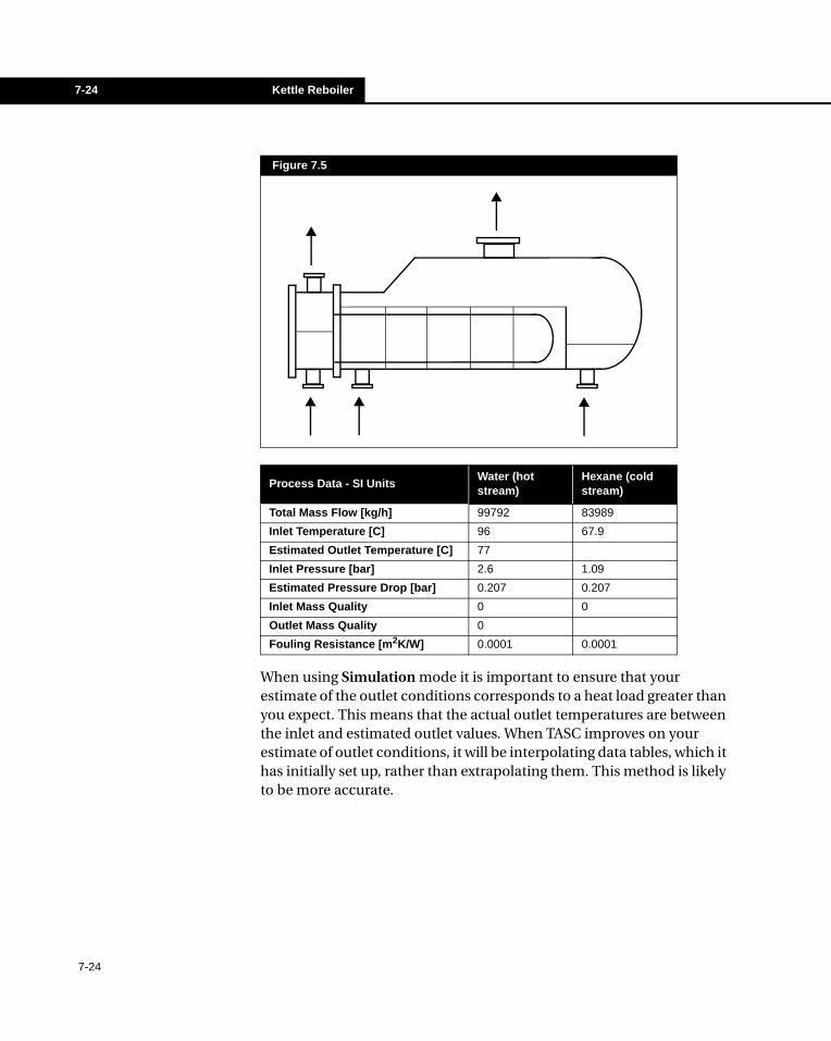
7-24 Kettle Reboiler

When using Simulation mode it is important to ensure that your estimate of the outlet conditions corresponds to a heat load greater than you expect. This means that the actual outlet temperatures are between the inlet and estimated outlet values. When TASC improves on your estimate of outlet conditions, it will be interpolating data tables, which it has initially set up, rather than extrapolating them. This method is likely to be more accurate.

Figure 7.5

Process Data - SI UnitsWater (hot stream)

Hexane (cold stream)

Total Mass Flow [kg/h] 99792 83989

Inlet Temperature [C] 96 67.9

Estimated Outlet Temperature [C] 77

Inlet Pressure [bar] 2.6 1.09

Estimated Pressure Drop [bar] 0.207 0.207

Inlet Mass Quality 0 0

Outlet Mass Quality 0

Fouling Resistance [m2K/W] 0.0001 0.0001

7-24

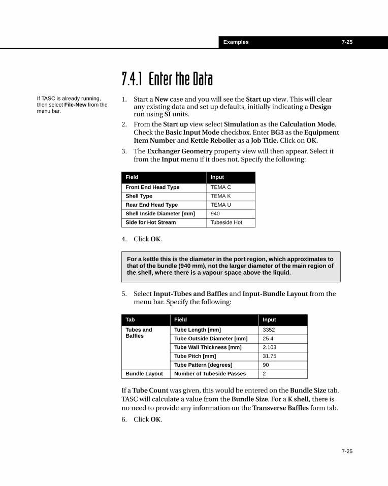
Examples 7-25

7.4.1 Enter the Data1. Start a New case and you will see the Start up view. This will clear

any existing data and set up defaults, initially indicating a Design run using SI units.

2. From the Start up view select Simulation as the Calculation Mode. Check the Basic Input Mode checkbox. Enter BG3 as the Equipment Item Number and Kettle Reboiler as a Job Title. Click on OK.

3. The Exchanger Geometry property view will then appear. Select it from the Input menu if it does not. Specify the following:

4. Click OK.

5. Select Input-Tubes and Baffles and Input-Bundle Layout from the menu bar. Specify the following:

If a Tube Count was given, this would be entered on the Bundle Size tab. TASC will calculate a value from the Bundle Size. For a K shell, there is no need to provide any information on the Transverse Baffles form tab.

6. Click OK.

Field Input

Front End Head Type TEMA C

Shell Type TEMA K

Rear End Head Type TEMA U

Shell Inside Diameter [mm] 940

Side for Hot Stream Tubeside Hot

For a kettle this is the diameter in the port region, which approximates to that of the bundle (940 mm), not the larger diameter of the main region of the shell, where there is a vapour space above the liquid.

Tab Field Input

Tubes and Baffles

Tube Length [mm] 3352

Tube Outside Diameter [mm] 25.4

Tube Wall Thickness [mm] 2.108

Tube Pitch [mm] 31.75

Tube Pattern [degrees] 90

Bundle Layout Number of Tubeside Passes 2

If TASC is already running, then select File-New from the menu bar.

7-25

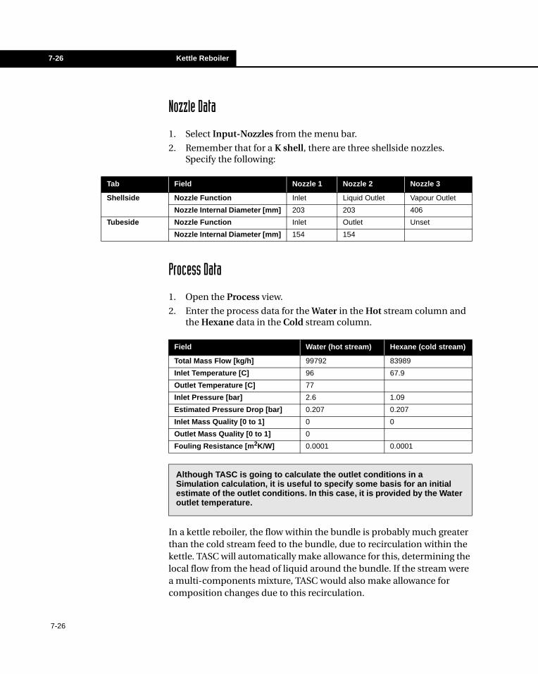
7-26 Kettle Reboiler

Nozzle Data

1. Select Input-Nozzles from the menu bar.

2. Remember that for a K shell, there are three shellside nozzles. Specify the following:

Process Data

1. Open the Process view.

2. Enter the process data for the Water in the Hot stream column and the Hexane data in the Cold stream column.

In a kettle reboiler, the flow within the bundle is probably much greater than the cold stream feed to the bundle, due to recirculation within the kettle. TASC will automatically make allowance for this, determining the local flow from the head of liquid around the bundle. If the stream were a multi-components mixture, TASC would also make allowance for composition changes due to this recirculation.

Tab Field Nozzle 1 Nozzle 2 Nozzle 3

Shellside Nozzle Function Inlet Liquid Outlet Vapour Outlet

Nozzle Internal Diameter [mm] 203 203 406

Tubeside Nozzle Function Inlet Outlet Unset

Nozzle Internal Diameter [mm] 154 154

Field Water (hot stream) Hexane (cold stream)

Total Mass Flow [kg/h] 99792 83989

Inlet Temperature [C] 96 67.9

Outlet Temperature [C] 77

Inlet Pressure [bar] 2.6 1.09

Estimated Pressure Drop [bar] 0.207 0.207

Inlet Mass Quality [0 to 1] 0 0

Outlet Mass Quality [0 to 1] 0

Fouling Resistance [m2K/W] 0.0001 0.0001

Although TASC is going to calculate the outlet conditions in a Simulation calculation, it is useful to specify some basis for an initial estimate of the outlet conditions. In this case, it is provided by the Water outlet temperature.

7-26

Examples 7-27

3. Select Input-Physical Properties from the menu bar.

4. The first form is for the Hot stream. This is Water, so under Stream Data Source click on Water (NEL40). This will cause data for water to be obtained from the NEL40 databank when the program is run.

5. Click on the Cold Stream tab. Enter the Stream Name as Hexane and set the Stream Type to Hydrocarbon. Under Stream Data Source click on Add. You will see a component selection list. Double-click on n-hexane and it will move to the Selected Components list.

6. The status bar at the bottom right corner of the view should be green and show Ready to indicate that the components and property methods have been set. If you click on the Property Package tab you will see that Peng Robinson for both phases has been selected, as a consequence of defining the Stream Type as Hydrocarbon.

7. Close the Data Source view, and on the main Properties view, you will see that your new data source, named Hyrocarbon 1, has been selected for stream 2 (hexane). Since the stream is a pure component, the composition default (1.0) is correct.

8. Click on Options. Check that a temperature range for properties is set. If not set, enter the two values: 67-96 that will cover the range possible in the exchanger. Close the Options view.

9. On the main Properties view click on Get Properties. You will see the property values for hexane appear on the spreadsheet.

10. Close the Physical Properties view.

11. The file should now be saved. Select File-Save As from the menu bar in the TASC desktop.

12. In the Save As view, specify BG3.TAI for the file name.

13. You have now entered all the data that is required and can run TASC calculations by clicking on the Run icon, or by selecting Run-Calculate All from the menu bar.Run icon

7-27

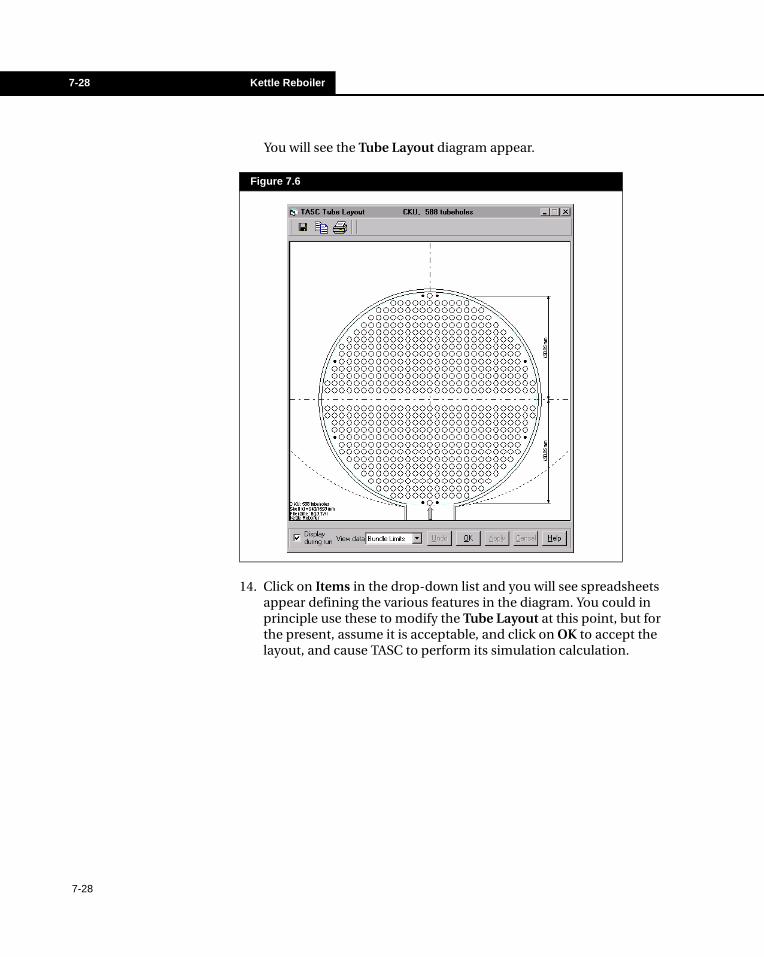
7-28 Kettle Reboiler

You will see the Tube Layout diagram appear.

14. Click on Items in the drop-down list and you will see spreadsheets appear defining the various features in the diagram. You could in principle use these to modify the Tube Layout at this point, but for the present, assume it is acceptable, and click on OK to accept the layout, and cause TASC to perform its simulation calculation.

Figure 7.6

7-28

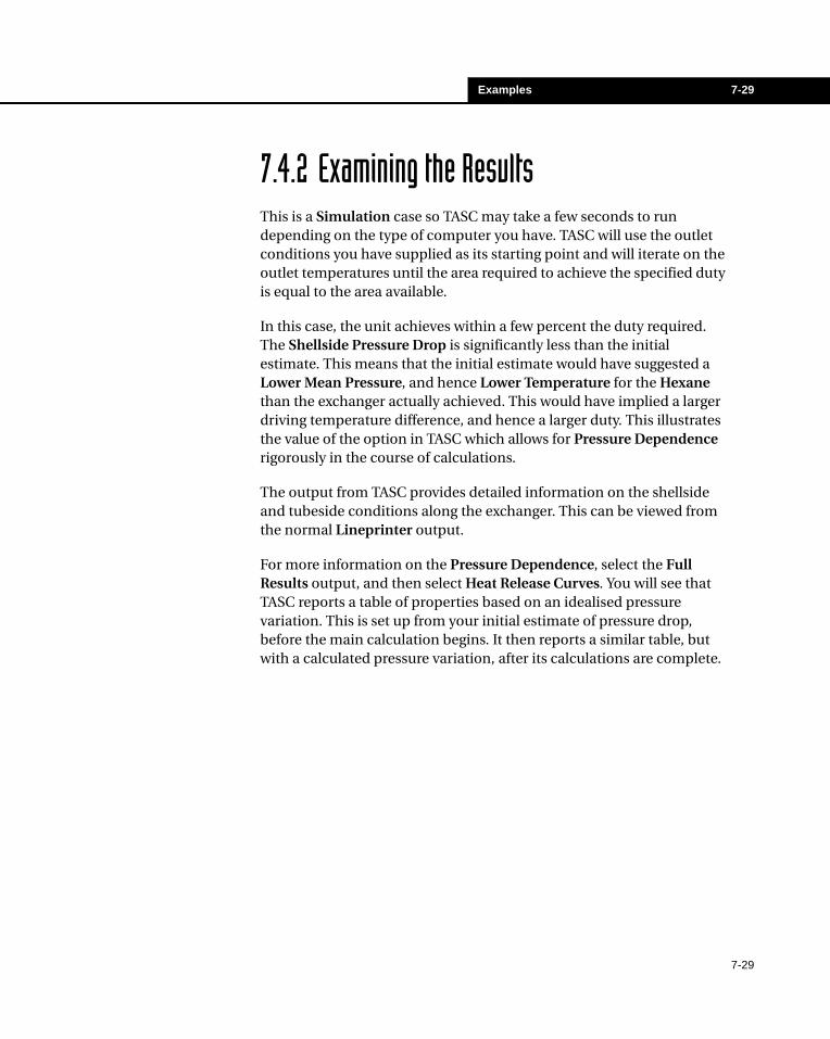
Examples 7-29

7.4.2 Examining the ResultsThis is a Simulation case so TASC may take a few seconds to run depending on the type of computer you have. TASC will use the outlet conditions you have supplied as its starting point and will iterate on the outlet temperatures until the area required to achieve the specified duty is equal to the area available.

In this case, the unit achieves within a few percent the duty required. The Shellside Pressure Drop is significantly less than the initial estimate. This means that the initial estimate would have suggested a Lower Mean Pressure, and hence Lower Temperature for the Hexane than the exchanger actually achieved. This would have implied a larger driving temperature difference, and hence a larger duty. This illustrates the value of the option in TASC which allows for Pressure Dependence rigorously in the course of calculations.

The output from TASC provides detailed information on the shellside and tubeside conditions along the exchanger. This can be viewed from the normal Lineprinter output.

For more information on the Pressure Dependence, select the Full Results output, and then select Heat Release Curves. You will see that TASC reports a table of properties based on an idealised pressure variation. This is set up from your initial estimate of pressure drop, before the main calculation begins. It then reports a similar table, but with a calculated pressure variation, after its calculations are complete.

7-29

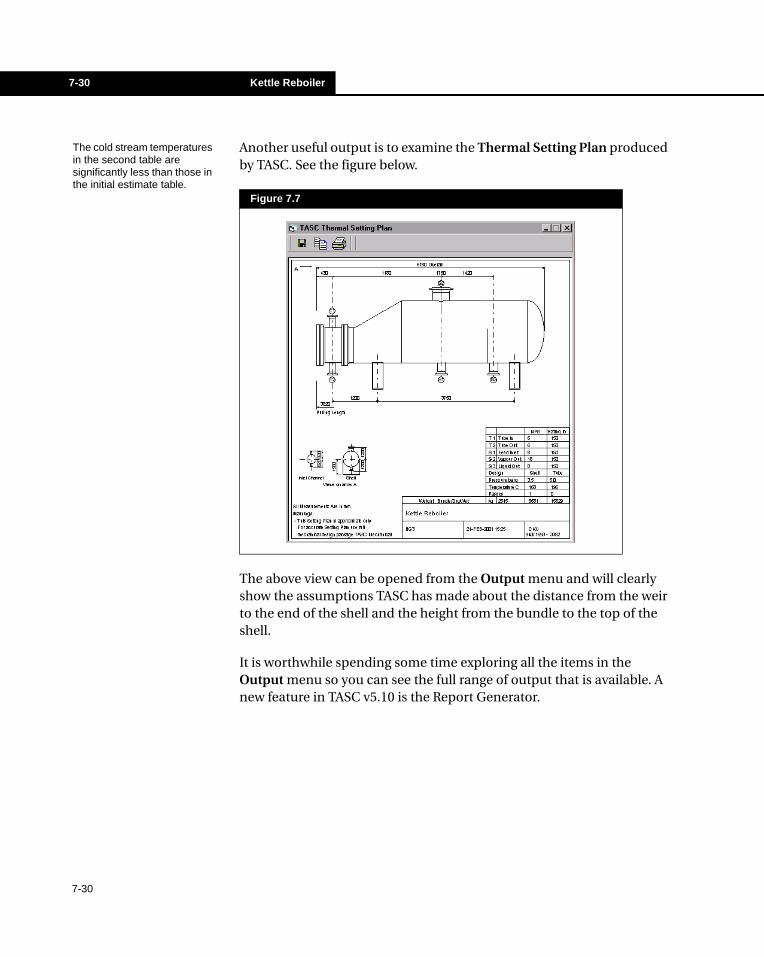
7-30 Kettle Reboiler

Another useful output is to examine the Thermal Setting Plan produced by TASC. See the figure below.

The above view can be opened from the Output menu and will clearly show the assumptions TASC has made about the distance from the weir to the end of the shell and the height from the bundle to the top of the shell.

It is worthwhile spending some time exploring all the items in the Output menu so you can see the full range of output that is available. A new feature in TASC v5.10 is the Report Generator.

Figure 7.7

The cold stream temperatures in the second table are significantly less than those in the initial estimate table.

7-30

Examples 7-31

7.5 Falling Film EvaporatorThis example will be used to illustrate the use of TASC to Rate (Check) a Falling Film Evaporator. Hence, for a checking case, the geometry of the exchanger and the process conditions are known and you want TASC to help determine if the exchanger can achieve the required duty.

This example uses condensing steam on the shellside to evaporate a falling film of 5% Brine on the tubeside. The data have been provided in British/American Customary units. Details of the exchanger are given below. It is a single exchanger made of carbon steel.

Geometric Data Value

TEMA Designation AEL

Shell Diameter [in] 27.5

Shell Orientation Vertical

Shellside Nozzle Diameter Inlet [in] 6

Shellside Nozzle Diameter Outlet [in] 4

Tubeside Nozzle Diameter Inlet [in] 4

Tubeside Nozzle Diameter Outlet [in] 8

Tube Length [in] 180

Tube Outside Diameter [in] 2

Tube Wall Thickness [in] 0.083

Tube Pitch [in] 2.5

Tube Pattern [degrees] 60

Tubeside Passes 1

Baffle Pitch [in] 7.875

Baffle Thickness [in] 0.375

Baffle Cut [%] 40%

Number of Baffles 20

This example utilises British/American units.

7-31

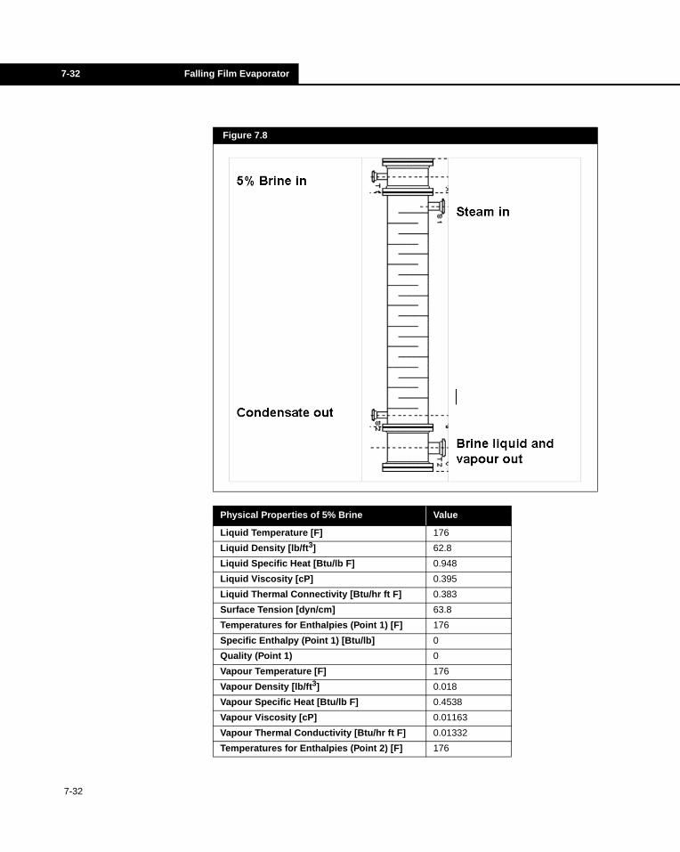
7-32 Falling Film Evaporator

Figure 7.8

Physical Properties of 5% Brine Value

Liquid Temperature [F] 176

Liquid Density [lb/ft3] 62.8

Liquid Specific Heat [Btu/lb F] 0.948

Liquid Viscosity [cP] 0.395

Liquid Thermal Connectivity [Btu/hr ft F] 0.383

Surface Tension [dyn/cm] 63.8

Temperatures for Enthalpies (Point 1) [F] 176

Specific Enthalpy (Point 1) [Btu/lb] 0

Quality (Point 1) 0

Vapour Temperature [F] 176

Vapour Density [lb/ft3] 0.018

Vapour Specific Heat [Btu/lb F] 0.4538

Vapour Viscosity [cP] 0.01163

Vapour Thermal Conductivity [Btu/hr ft F] 0.01332

Temperatures for Enthalpies (Point 2) [F] 176

7-32

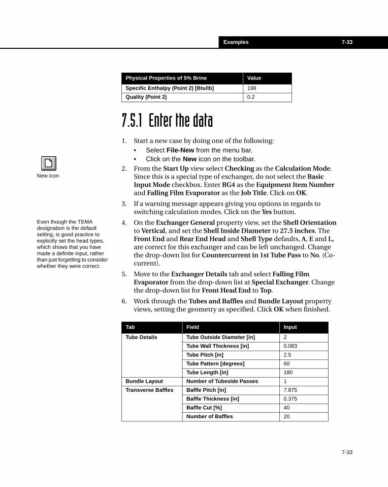
Examples 7-33

7.5.1 Enter the data1. Start a new case by doing one of the following:

• Select File-New from the menu bar.• Click on the New icon on the toolbar.

2. From the Start Up view select Checking as the Calculation Mode. Since this is a special type of exchanger, do not select the Basic Input Mode checkbox. Enter BG4 as the Equipment Item Number and Falling Film Evaporator as the Job Title. Click on OK.

3. If a warning message appears giving you options in regards to switching calculation modes. Click on the Yes button.

4. On the Exchanger General property view, set the Shell Orientation to Vertical, and set the Shell Inside Diameter to 27.5 inches. The Front End and Rear End Head and Shell Type defaults, A, E and L, are correct for this exchanger and can be left unchanged. Change the drop-down list for Countercurrent in 1st Tube Pass to No. (Co-current).

5. Move to the Exchanger Details tab and select Falling Film Evaporator from the drop-down list at Special Exchanger. Change the drop-down list for Front Head End to Top.

6. Work through the Tubes and Baffles and Bundle Layout property views, setting the geometry as specified. Click OK when finished.

Specific Enthalpy (Point 2) [Btu/lb] 198

Quality (Point 2) 0.2

Tab Field Input

Tube Details Tube Outside Diameter [in] 2

Tube Wall Thickness [in] 0.083

Tube Pitch [in] 2.5

Tube Pattern [degrees] 60

Tube Length [in] 180

Bundle Layout Number of Tubeside Passes 1

Transverse Baffles Baffle Pitch [in] 7.875

Baffle Thickness [in] 0.375

Baffle Cut [%] 40

Number of Baffles 20

Physical Properties of 5% Brine Value

New icon

Even though the TEMA designation is the default setting, is good practice to explicitly set the head types, which shows that you have made a definite input, rather than just forgetting to consider whether they were correct.

7-33

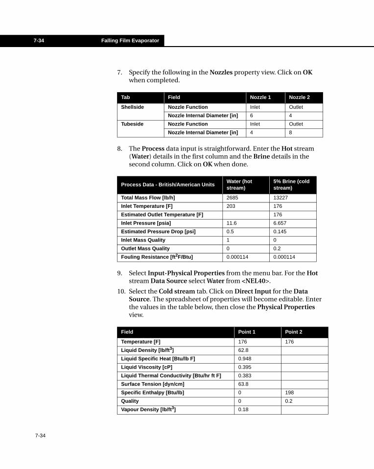
7-34 Falling Film Evaporator

7. Specify the following in the Nozzles property view. Click on OK when completed.

8. The Process data input is straightforward. Enter the Hot stream (Water) details in the first column and the Brine details in the second column. Click on OK when done.

9. Select Input-Physical Properties from the menu bar. For the Hot stream Data Source select Water from <NEL40>.

10. Select the Cold stream tab. Click on Direct Input for the Data Source. The spreadsheet of properties will become editable. Enter the values in the table below, then close the Physical Properties view.

Tab Field Nozzle 1 Nozzle 2

Shellside Nozzle Function Inlet Outlet

Nozzle Internal Diameter [in] 6 4

Tubeside Nozzle Function Inlet Outlet

Nozzle Internal Diameter [in] 4 8

Process Data - British/American UnitsWater (hot stream)

5% Brine (cold stream)

Total Mass Flow [lb/h] 2685 13227

Inlet Temperature [F] 203 176

Estimated Outlet Temperature [F] 176

Inlet Pressure [psia] 11.6 6.657

Estimated Pressure Drop [psi] 0.5 0.145

Inlet Mass Quality 1 0

Outlet Mass Quality 0 0.2

Fouling Resistance [ft2F/Btu] 0.000114 0.000114

Field Point 1 Point 2

Temperature [F] 176 176

Liquid Density [lb/ft3] 62.8

Liquid Specific Heat [Btu/lb F] 0.948

Liquid Viscosity [cP] 0.395

Liquid Thermal Conductivity [Btu/hr ft F] 0.383

Surface Tension [dyn/cm] 63.8

Specific Enthalpy [Btu/lb] 0 198

Quality 0 0.2

Vapour Density [lb/ft3] 0.18

7-34

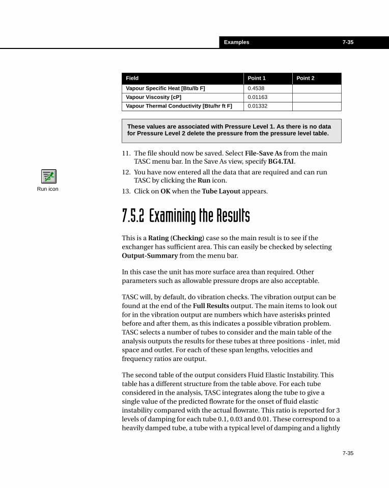
Examples 7-35

11. The file should now be saved. Select File-Save As from the main TASC menu bar. In the Save As view, specify BG4.TAI.

12. You have now entered all the data that are required and can run TASC by clicking the Run icon.

13. Click on OK when the Tube Layout appears.

7.5.2 Examining the ResultsThis is a Rating (Checking) case so the main result is to see if the exchanger has sufficient area. This can easily be checked by selecting Output-Summary from the menu bar.

In this case the unit has more surface area than required. Other parameters such as allowable pressure drops are also acceptable.

TASC will, by default, do vibration checks. The vibration output can be found at the end of the Full Results output. The main items to look out for in the vibration output are numbers which have asterisks printed before and after them, as this indicates a possible vibration problem. TASC selects a number of tubes to consider and the main table of the analysis outputs the results for these tubes at three positions - inlet, mid space and outlet. For each of these span lengths, velocities and frequency ratios are output.

The second table of the output considers Fluid Elastic Instability. This table has a different structure from the table above. For each tube considered in the analysis, TASC integrates along the tube to give a single value of the predicted flowrate for the onset of fluid elastic instability compared with the actual flowrate. This ratio is reported for 3 levels of damping for each tube 0.1, 0.03 and 0.01. These correspond to a heavily damped tube, a tube with a typical level of damping and a lightly

Vapour Specific Heat [Btu/lb F] 0.4538

Vapour Viscosity [cP] 0.01163

Vapour Thermal Conductivity [Btu/hr ft F] 0.01332

These values are associated with Pressure Level 1. As there is no data for Pressure Level 2 delete the pressure from the pressure level table.

Field Point 1 Point 2

Run icon

7-35

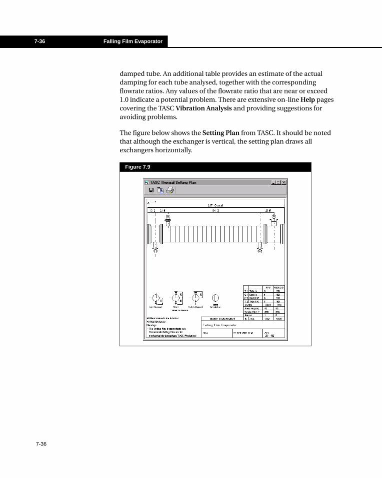
7-36 Falling Film Evaporator

damped tube. An additional table provides an estimate of the actual damping for each tube analysed, together with the corresponding flowrate ratios. Any values of the flowrate ratio that are near or exceed 1.0 indicate a potential problem. There are extensive on-line Help pages covering the TASC Vibration Analysis and providing suggestions for avoiding problems.

The figure below shows the Setting Plan from TASC. It should be noted that although the exchanger is vertical, the setting plan draws all exchangers horizontally.

Figure 7.9

7-36

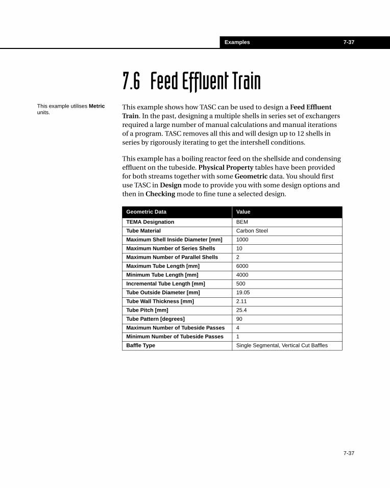
Examples 7-37

7.6 Feed Effluent TrainThis example shows how TASC can be used to design a Feed Effluent Train. In the past, designing a multiple shells in series set of exchangers required a large number of manual calculations and manual iterations of a program. TASC removes all this and will design up to 12 shells in series by rigorously iterating to get the intershell conditions.

This example has a boiling reactor feed on the shellside and condensing effluent on the tubeside. Physical Property tables have been provided for both streams together with some Geometric data. You should first use TASC in Design mode to provide you with some design options and then in Checking mode to fine tune a selected design.

Geometric Data Value

TEMA Designation BEM

Tube Material Carbon Steel

Maximum Shell Inside Diameter [mm] 1000

Maximum Number of Series Shells 10

Maximum Number of Parallel Shells 2

Maximum Tube Length [mm] 6000

Minimum Tube Length [mm] 4000

Incremental Tube Length [mm] 500

Tube Outside Diameter [mm] 19.05

Tube Wall Thickness [mm] 2.11

Tube Pitch [mm] 25.4

Tube Pattern [degrees] 90

Maximum Number of Tubeside Passes 4

Minimum Number of Tubeside Passes 1

Baffle Type Single Segmental, Vertical Cut Baffles

This example utilises Metric units.

7-37

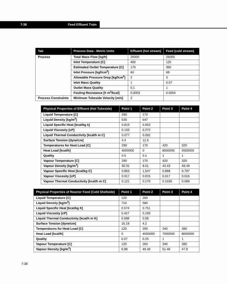
7-38 Feed Effluent Train

Tab Process Data - Metric Units Effluent (hot stream) Feed (cold stream)

Process Total Mass Flow [kg/h] 26000 26000

Inlet Temperature [C] 400 120

Estimated Outlet Temperature [C] 170 360

Inlet Pressure [kgf/cm2] 60 68

Allowable Pressure Drop [kgf/cm2] 2 3

Inlet Mass Quality 1 0.07

Outlet Mass Quality 0.1 1

Fouling Resistance [h m2/kcal] 0.0003 0.0004

Process Constraints Minimum Tubeside Velocity [m/s] 2

Physical Properties of Effluent (Hot Tubeside) Point 1 Point 2 Point 3 Point 4

Liquid Temperature [C] 290 170

Liquid Density [kg/m3] 535 647

Liquid Specific Heat [kcal/kg k] 0.815 0.653

Liquid Viscosity [cP] 0.155 0.272

Liquid Thermal Conductivity [kcal/h m C] 0.077 0.092

Surface Tension [dyne/cm] 4.4 11.5

Temperatures for Heat Load [C] 290 170 420 320

Heat Load [kcal/h] 4000000 0 8000000 5500000

Quality 0.5 0.1 1 1

Vapour Temperature [C] 290 170 420 320

Vapour Density [kg/m3] 30.31 8.01 43.43 49.49

Vapour Specific Heat [kcal/kg C] 0.853 1.547 0.868 0.797

Vapour Viscosity [cP] 0.017 0.015 0.017 0.016

Vapour Thermal Conductivity [kcal/h m C] 0.121 0.176 0.1036 0.089

Physical Properties of Reactor Feed (Cold Shellside) Point 1 Point 2 Point 3 Point 4

Liquid Temperature [C] 120 260

Liquid Density [kg/m3] 710 580

Liquid Specific Heat [kcal/kg K] 0.574 0.751

Liquid Viscosity [cP] 0.427 0.183

Liquid Thermal Conductivity [kcal/h m K] 0.098 0.08

Surface Tension [dyne/cm] 16.19 4.2

Temperatures for Heat Load [C] 120 260 340 380

Heat Load [kcal/h] 0 4000000 7000000 8000000

Quality 0.07 0.25 1 1

Vapour Temperature [C] 120 260 340 380

Vapour Density [kg/m3] 6.98 49.49 51.46 47.8

7-38

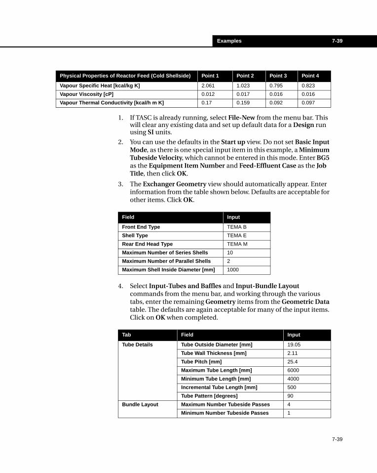
Examples 7-39

1. If TASC is already running, select File-New from the menu bar. This will clear any existing data and set up default data for a Design run using SI units.

2. You can use the defaults in the Start up view. Do not set Basic Input Mode, as there is one special input item in this example, a Minimum Tubeside Velocity, which cannot be entered in this mode. Enter BG5 as the Equipment Item Number and Feed-Effluent Case as the Job Title, then click OK.

3. The Exchanger Geometry view should automatically appear. Enter information from the table shown below. Defaults are acceptable for other items. Click OK.

4. Select Input-Tubes and Baffles and Input-Bundle Layout commands from the menu bar, and working through the various tabs, enter the remaining Geometry items from the Geometric Data table. The defaults are again acceptable for many of the input items. Click on OK when completed.

Vapour Specific Heat [kcal/kg K] 2.061 1.023 0.795 0.823

Vapour Viscosity [cP] 0.012 0.017 0.016 0.016

Vapour Thermal Conductivity [kcal/h m K] 0.17 0.159 0.092 0.097

Physical Properties of Reactor Feed (Cold Shellside) Point 1 Point 2 Point 3 Point 4

Field Input

Front End Type TEMA B

Shell Type TEMA E

Rear End Head Type TEMA M

Maximum Number of Series Shells 10

Maximum Number of Parallel Shells 2

Maximum Shell Inside Diameter [mm] 1000

Tab Field Input

Tube Details Tube Outside Diameter [mm] 19.05

Tube Wall Thickness [mm] 2.11

Tube Pitch [mm] 25.4

Maximum Tube Length [mm] 6000

Minimum Tube Length [mm] 4000

Incremental Tube Length [mm] 500

Tube Pattern [degrees] 90

Bundle Layout Maximum Number Tubeside Passes 4

Minimum Number Tubeside Passes 1

7-39

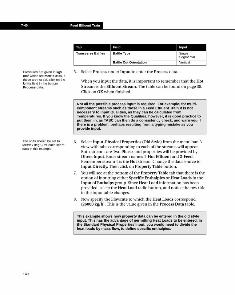
7-40 Feed Effluent Train

5. Select Process under Input to enter the Process data.

When you input the data, it is important to remember that the Hot Stream is the Effluent Stream. The table can be found on page 38. Click on OK when finished.

6. Select Input-Physical Properties (Old Style) from the menu bar. A view with tabs corresponding to each of the streams will appear. Both streams are Two Phase, and properties will be provided by Direct Input. Enter stream names 1-Hot Effluent and 2-Feed. Remember stream 1 is the Hot stream. Change the data source to Input Directly. Then click on Property Table button.

7. You will see at the bottom of the Property Table tab that there is the option of inputting either Specific Enthalpies or Heat Loads in the Input of Enthalpy group. Since Heat Load information has been provided, select the Heat Load radio button, and notice the row title in the input table changes.

8. Now specify the Flowrate to which the Heat Loads correspond (26000 kg/h). This is the value given in the Process Data table.

Transverse Baffles Baffle Type Single Segmental

Baffle Cut Orientation Vertical

Not all the possible process input is required. For example, for multi-component streams such as those in a Feed Effluent Train it is not necessary to input Qualities, as they can be calculated from Temperatures. If you know the Qualities, however, it is good practice to put them in, as TASC can then do a consistency check, and warn you if there is a problem, perhaps resulting from a typing mistake as you provide input.

This example shows how property data can be entered in the old style input. This has the advantage of permitting Heat Loads to be entered. In the Standard Physical Properties Input, you would need to divide the heat loads by mass flow, to define specific enthalpies.

Tab Field Input

Pressures are given in kgf/cm2 which are metric units. If these are not set, click on the Units field in the bottom Process data.

The units should be set to Metric / deg C for each set of data in this example.

7-40

Examples 7-41

9. Enter all the Properties for the Effluent and click OK when completed. The table of values can be found on page 38.

10. Move to the tab for Stream 2, click on the Properties Table button and proceed to enter the feed stream properties, click on the Heat Load radio button, and specify the Flowrate. Click OK when completed. The table can be found on page 38.

11. You have now entered all the data that are required. Run TASC Calculations by clicking on the Run icon, or select Run-Calculate All from the menu bar.

12. When you click Run you are asked if you want to save the input file. If you want a permanent record of the input at this stage click Yes, otherwise click No. The program will still run the data you have just input.

As this is a Design case no Tube Layout will appear. Since you have asked the program to consider up to ten shells in series, the program may take several minutes to run. This is because TASC performs a rigorous iteration to establish the intershell conditions (it does not use a simple stepping off method).

There are three sets of properties, Liquid, T-h-x and Vapour, each with their own set of Temperatures. The properties may be entered in any order, hot to cold or cold to hot, but remember to begin each set in the leftmost column.

Run icon

7-41

7-42 Feed Effluent Train

7.6.1 Examining the ResultsWhen TASC has completed its calculations a Summary of the results appears automatically. A list of any Error or Warning messages will also be shown.

A warning has been issued as heat loads have been input as opposed to the better option of the input of specific enthalpies. A warning has been issued concerning the mean error in interpolating T-H data. This is due to few data points being input.

TASC has issued a Warning with regards to Two Phase on the Tubeside. In Design mode TASC simplifies the Tubeside Temperature Profile calculation and so TASC recommends that you optimise the design

further using Rating (Checking) as this removes the simplifying assumptions that are made with Two Phase on the Tubeside.

TASC will have considered a range of designs and by default, will have reported on any valid designs within 25% of the relative lowest cost design. The list of designs considered can be viewed by selecting Output-Alternative Designs from the menu bar.

7-42

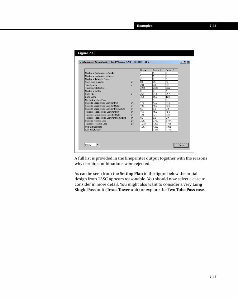
Examples 7-43

A full list is provided in the lineprinter output together with the reasons why certain combinations were rejected.

As can be seen from the Setting Plan in the figure below the initial design from TASC appears reasonable. You should now select a case to consider in more detail. You might also want to consider a very Long Single Pass unit (Texas Tower unit) or explore the Two Tube Pass case.

Figure 7.10

7-43

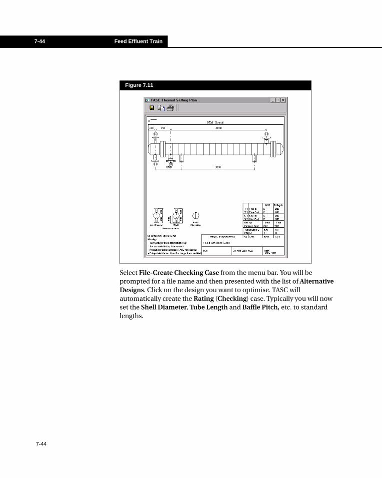
7-44 Feed Effluent Train

Select File-Create Checking Case from the menu bar. You will be prompted for a file name and then presented with the list of Alternative Designs. Click on the design you want to optimise. TASC will automatically create the Rating (Checking) case. Typically you will now set the Shell Diameter, Tube Length and Baffle Pitch, etc. to standard lengths.

Figure 7.11

7-44

Examples 7-45

7.7 Vertical Thermosyphon ReboilerThe TASC Thermosyphon mode can handle tubeside boiling in vertical TEMA type E or X shells, shellside boiling in vertical E shells, and shellside boiling in Horizontal E, F, G, H, J, I and X shells. It can also handle tubeside or shellside boiling in vertical double-pipe exchangers with a single leg.

The Thermosyphon option provides a Simulation of a specified exchanger geometry, and the pipework connecting it to the distillation column. The Flowrate of the Boiling Thermosyphon stream is determined by the Driving Gravitational head and the Resistance to flow in the exchanger and pipework.

The first stage in simulating any reboiler is to make a sketch including the reboiler, the bottom of the distillation column and the connecting pipework. Notice the various heights and lengths on this sketch together with Pipe/Nozzle Diameters. For a complex inlet line of constant diameter, you only need to know the Total Length of the line and the Number of Bends. If the line branches to feed more than one exchanger, or to connect to two nozzles on an H-shell, you need to observe the Average Length of line and Number of Bends, in each of the parallel paths.

The Outlet/Return line is usually relatively simple. You should observe the length and diameter of each horizontal or vertical section of this line, as well as the presence of any bends in the line.

Various important heights, which need to be input for determining Gravitational Effects in a Reboiler, must be defined relative to a datum. Any datum may be used, provided that the same one is used for all these input items.

This example utilises SI units.

7-45

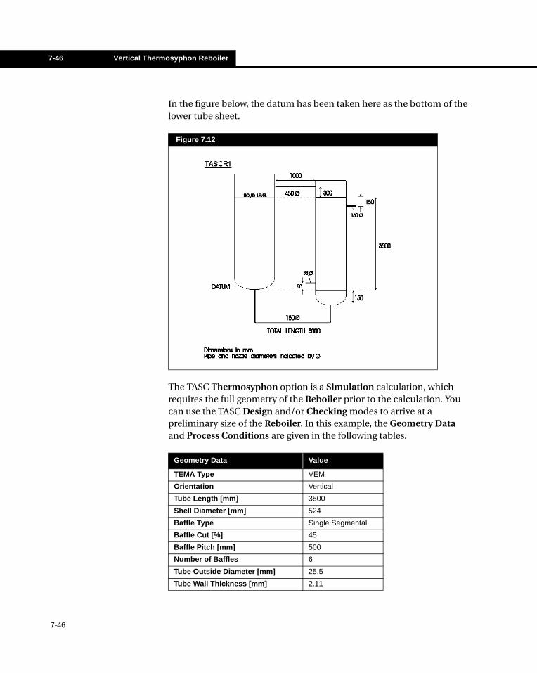
7-46 Vertical Thermosyphon Reboiler

In the figure below, the datum has been taken here as the bottom of the lower tube sheet.

The TASC Thermosyphon option is a Simulation calculation, which requires the full geometry of the Reboiler prior to the calculation. You can use the TASC Design and/or Checking modes to arrive at a preliminary size of the Reboiler. In this example, the Geometry Data and Process Conditions are given in the following tables.

Figure 7.12

Geometry Data Value

TEMA Type VEM

Orientation Vertical

Tube Length [mm] 3500

Shell Diameter [mm] 524

Baffle Type Single Segmental

Baffle Cut [%] 45

Baffle Pitch [mm] 500

Number of Baffles 6

Tube Outside Diameter [mm] 25.5

Tube Wall Thickness [mm] 2.11

7-46

Examples 7-47

The Cold stream composition is known so COMThermo can be used to calculate its properties.

With the sketch in Figure 7.12 and the tables, we now have enough information to start setting up an input file for TASC.

Pitch Ratio 1.25

Tube Layout [degrees] 30

Process Conditions Shellside Hot Tubeside Cold

Stream Steam Debutanizer Bottoms

Inlet Temperatures [C]

Pressure in Column [bar] 5.2

Operating Pressure [bar] 3.5 5.2 (approx)

Fouling Resistance [m2K/W] 0.000088 0.0001

Component Mass Fraction

1,3 Butadiene 0.02

Pentane 0.71

Benzene 0.27

Geometry Data Value

7-47

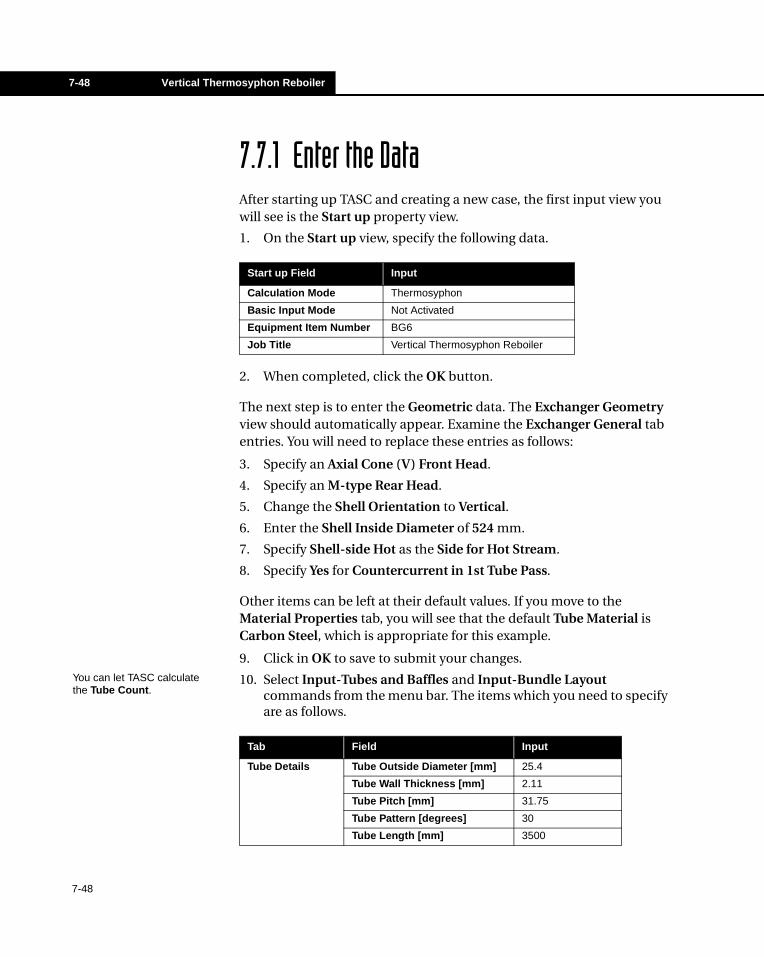
7-48 Vertical Thermosyphon Reboiler

7.7.1 Enter the DataAfter starting up TASC and creating a new case, the first input view you will see is the Start up property view.

1. On the Start up view, specify the following data.

2. When completed, click the OK button.

The next step is to enter the Geometric data. The Exchanger Geometry view should automatically appear. Examine the Exchanger General tab entries. You will need to replace these entries as follows:

3. Specify an Axial Cone (V) Front Head.

4. Specify an M-type Rear Head.

5. Change the Shell Orientation to Vertical.

6. Enter the Shell Inside Diameter of 524 mm.

7. Specify Shell-side Hot as the Side for Hot Stream.

8. Specify Yes for Countercurrent in 1st Tube Pass.

Other items can be left at their default values. If you move to the Material Properties tab, you will see that the default Tube Material is Carbon Steel, which is appropriate for this example.

9. Click in OK to save to submit your changes.

10. Select Input-Tubes and Baffles and Input-Bundle Layout commands from the menu bar. The items which you need to specify are as follows.

Start up Field Input

Calculation Mode Thermosyphon

Basic Input Mode Not Activated

Equipment Item Number BG6

Job Title Vertical Thermosyphon Reboiler

Tab Field Input

Tube Details Tube Outside Diameter [mm] 25.4

Tube Wall Thickness [mm] 2.11

Tube Pitch [mm] 31.75

Tube Pattern [degrees] 30

Tube Length [mm] 3500

You can let TASC calculate the Tube Count.

7-48

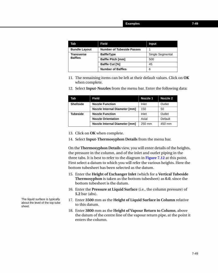
Examples 7-49

11. The remaining items can be left at their default values. Click on OK when complete.

12. Select Input-Nozzles from the menu bar. Enter the following data:

13. Click on OK when complete.

14. Select Input-Thermosyphon Details from the menu bar.

On the Thermosyphon Details view, you will enter details of the heights, the pressure in the column, and of the inlet and outlet piping in the three tabs. It is best to refer to the diagram in Figure 7.12 at this point. First select a datum to which you will refer the various heights. Here the bottom tubesheet has been selected as the datum.

15. Enter the Height of Exchanger Inlet (which for a Vertical Tubeside Thermosyphon is taken as the bottom tubesheet) as 0.0, since the bottom tubesheet is the datum.

16. Enter the Pressure at Liquid Surface (i.e., the column pressure) of 5.2 bar (abs).

17. Enter 3500 mm as the Height of Liquid Surface in Column relative to this datum.

18. Enter 3800 mm as the Height of Vapour Return to Column, above the datum of the centre line of the vapour return pipe, at the point it enters the column.

Bundle Layout Number of Tubeside Passes 1

Transverse Baffles

BaffleType Single Segmental

Baffle Pitch [mm] 500

Baffle Cut [%] 45

Number of Baffles 6

Tab Field Nozzle 1 Nozzle 2

Shellside Nozzle Function Inlet Outlet

Nozzle Internal Diameter [mm] 150 50

Tubeside Nozzle Function Inlet Outlet

Nozzle Orientation Axial Default

Nozzle Internal Diameter [mm] 250 mm 450 mm

Tab Field Input

The liquid surface is typically about the level of the top tube sheet.

7-49

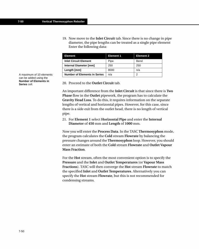
7-50 Vertical Thermosyphon Reboiler

19. Now move to the Inlet Circuit tab. Since there is no change in pipe diameter, the pipe lengths can be treated as a single pipe element Enter the following data:

20. Proceed to the Outlet Circuit tab.

An important difference from the Inlet Circuit is that since there is Two Phase flow in the Outlet pipework, the program has to calculate the Gravity Head Loss. To do this, it requires information on the separate lengths of vertical and horizontal pipes. However, for this case, since there is a side exit from the outlet head, there is no length of vertical pipe.

21. For Element 1 select Horizontal Pipe and enter the Internal Diameter of 450 mm and Length of 1000 mm.

Now you will enter the Process Data. In the TASC Thermosyphon mode, the program calculates the Cold stream Flowrate by balancing the pressure changes around the Thermosyphon loop. However, you should enter an estimate of both the Cold stream Flowrate and Outlet Vapour Mass Fraction.

For the Hot stream, often the most convenient option is to specify the Pressure and the Inlet and Outlet Temperatures (or Vapour Mass Fractions). TASC will then converge the Hot stream Flowrate to match the specified Inlet and Outlet Temperatures. Alternatively you can specify the Hot stream Flowrate, but this is not recommended for condensing streams.

Element Element 1 Element 2

Inlet Circuit Element Pipe Bend

Internal Diameter [mm] 250 250

Length [mm] 8000 n/a

Number of Elements in Series n/a 2A maximum of 10 elements can be added using the Number of Elements in Series cell.

7-50

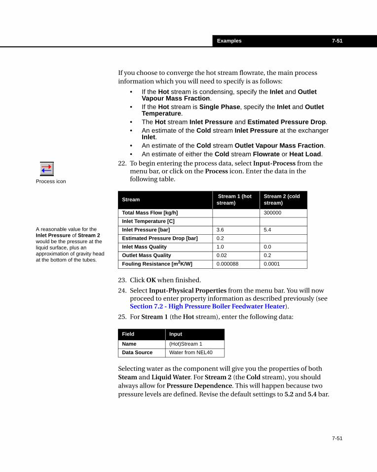
Examples 7-51

If you choose to converge the hot stream flowrate, the main process information which you will need to specify is as follows:

• If the Hot stream is condensing, specify the Inlet and Outlet Vapour Mass Fraction.

• If the Hot stream is Single Phase, specify the Inlet and Outlet Temperature.

• The Hot stream Inlet Pressure and Estimated Pressure Drop.• An estimate of the Cold stream Inlet Pressure at the exchanger

Inlet.• An estimate of the Cold stream Outlet Vapour Mass Fraction.• An estimate of either the Cold stream Flowrate or Heat Load.

22. To begin entering the process data, select Input-Process from the menu bar, or click on the Process icon. Enter the data in the following table.

23. Click OK when finished.

24. Select Input-Physical Properties from the menu bar. You will now proceed to enter property information as described previously (see Section 7.2 - High Pressure Boiler Feedwater Heater).

25. For Stream 1 (the Hot stream), enter the following data:

Selecting water as the component will give you the properties of both Steam and Liquid Water. For Stream 2 (the Cold stream), you should always allow for Pressure Dependence. This will happen because two pressure levels are defined. Revise the default settings to 5.2 and 5.4 bar.

Stream Stream 1 (hot stream)

Stream 2 (cold stream)

Total Mass Flow [kg/h] 300000

Inlet Temperature [C]

Inlet Pressure [bar] 3.6 5.4

Estimated Pressure Drop [bar] 0.2

Inlet Mass Quality 1.0 0.0

Outlet Mass Quality 0.02 0.2

Fouling Resistance [m2K/W] 0.000088 0.0001

Field Input

Name (Hot)Stream 1

Data Source Water from NEL40

Process icon

A reasonable value for the Inlet Pressure of Stream 2 would be the pressure at the liquid surface, plus an approximation of gravity head at the bottom of the tubes.

7-51

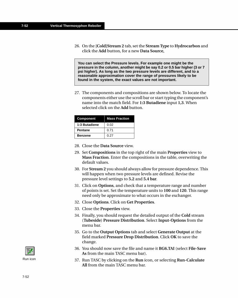
7-52 Vertical Thermosyphon Reboiler

26. On the [Cold]Stream 2 tab, set the Stream Type to Hydrocarbon and click the Add button, for a new Data Source.

27. The components and compositions are shown below. To locate the components either use the scroll bar or start typing the component’s name into the match field. For 1:3 Butadiene input 1,3. When selected click on the Add button.

28. Close the Data Source view.

29. Set Compositions in the top right of the main Properties view to Mass Fraction. Enter the compositions in the table, overwriting the default values.

30. For Stream 2 you should always allow for pressure dependence. This will happen when two pressure levels are defined. Revise the pressure level settings to 5.2 and 5.4 bar.

31. Click on Options, and check that a temperature range and number of points is set. Set the temperature units to 100 and 120. This range need only be approximate to what occurs in the exchanger.

32. Close Options. Click on Get Properties.

33. Close the Properties view.

34. Finally, you should request the detailed output of the Cold stream (Tubeside) Pressure Distribution. Select Input-Options from the menu bar.

35. Go to the Output Options tab and select Generate Output at the field marked Pressure Drop Distribution. Click OK to save the change.

36. You should now save the file and name it BG6.TAI (select File-Save As from the main TASC menu bar).

37. Run TASC by clicking on the Run icon, or selecting Run-Calculate All from the main TASC menu bar.

You can select the Pressure levels. For example one might be the pressure in the column, another might be say 0.2 or 0.5 bar higher (3 or 7 psi higher). As long as the two pressure levels are different, and to a reasonable approximation cover the range of pressures likely to be found in the system, the exact values are not important.

Component Mass Fraction

1:3 Butadiene 0.02

Pentane 0.71

Benzene 0.27

Run icon

7-52

Examples 7-53

38. Click on OK when the Tube Layout appears.

7.7.2 Examining the ResultsDepending on the accuracy of your initial estimates, thermosyphon cases may take a few seconds to run. Be prepared for some cases to take longer.

The Results Summary will display the calculated Hot and Cold stream Flowrates, and the calculated Heat Load.

The Lineprinter output (opened by selecting Output-Line Printer from the menu bar) for the thermosyphon option will display some information, which is additional to the other TASC modes:

• The Table showing the cold stream properties with Calculated Pressure Variation will also show the conditions in the column. Points 1 to 12 cover the heat exchanger only, from Inlet to Outlet Nozzle.

• A Thermosyphon Circuit section shows a detailed printout of the Pressure Drop calculations in the Inlet and Outlet pipework.

• Information messages will be printed to inform you of the results of the Reboiler Stability Analysis.

• Just below the Nozzle output, you will find information on parameters, which assess whether or not the Vapour Velocity at Outlet is high enough to ensure steady circulation. Information on the predicted Two Phase flow pattern in the Outlet pipework is also printed.

• If you have requested the Tubeside Pressure Drop Distribution, you will see that the Inlet and Outlet piping distributions have been added to the Table marked Incremental Page 2. You can check that the sum of the entries under Total Pressure Drop is zero, indicating that the Thermosyphon iterations have successfully converged.

7-53

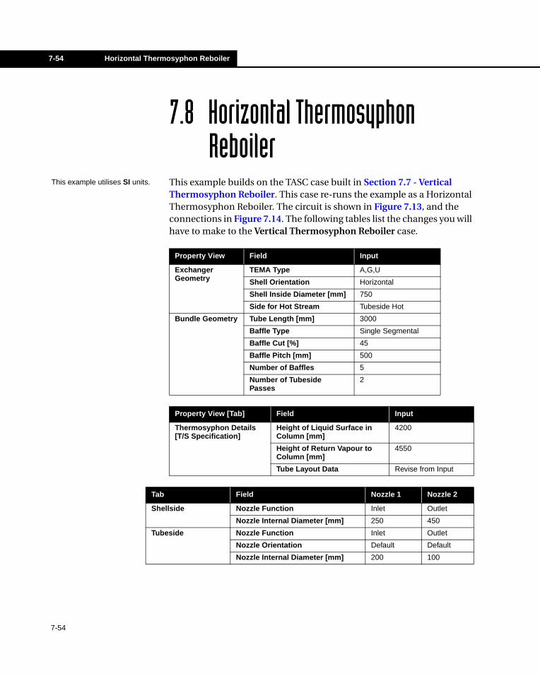
7-54 Horizontal Thermosyphon Reboiler

7.8 Horizontal Thermosyphon Reboiler

This example builds on the TASC case built in Section 7.7 - Vertical Thermosyphon Reboiler. This case re-runs the example as a Horizontal Thermosyphon Reboiler. The circuit is shown in Figure 7.13, and the connections in Figure 7.14. The following tables list the changes you will have to make to the Vertical Thermosyphon Reboiler case.

Property View Field Input

Exchanger Geometry

TEMA Type A,G,U

Shell Orientation Horizontal

Shell Inside Diameter [mm] 750

Side for Hot Stream Tubeside Hot

Bundle Geometry Tube Length [mm] 3000

Baffle Type Single Segmental

Baffle Cut [%] 45

Baffle Pitch [mm] 500

Number of Baffles 5

Number of Tubeside Passes

2

Property View [Tab] Field Input

Thermosyphon Details [T/S Specification]

Height of Liquid Surface in Column [mm]

4200

Height of Return Vapour to Column [mm]

4550

Tube Layout Data Revise from Input

Tab Field Nozzle 1 Nozzle 2

Shellside Nozzle Function Inlet Outlet

Nozzle Internal Diameter [mm] 250 450

Tubeside Nozzle Function Inlet Outlet

Nozzle Orientation Default Default

Nozzle Internal Diameter [mm] 200 100

This example utilises SI units.

7-54

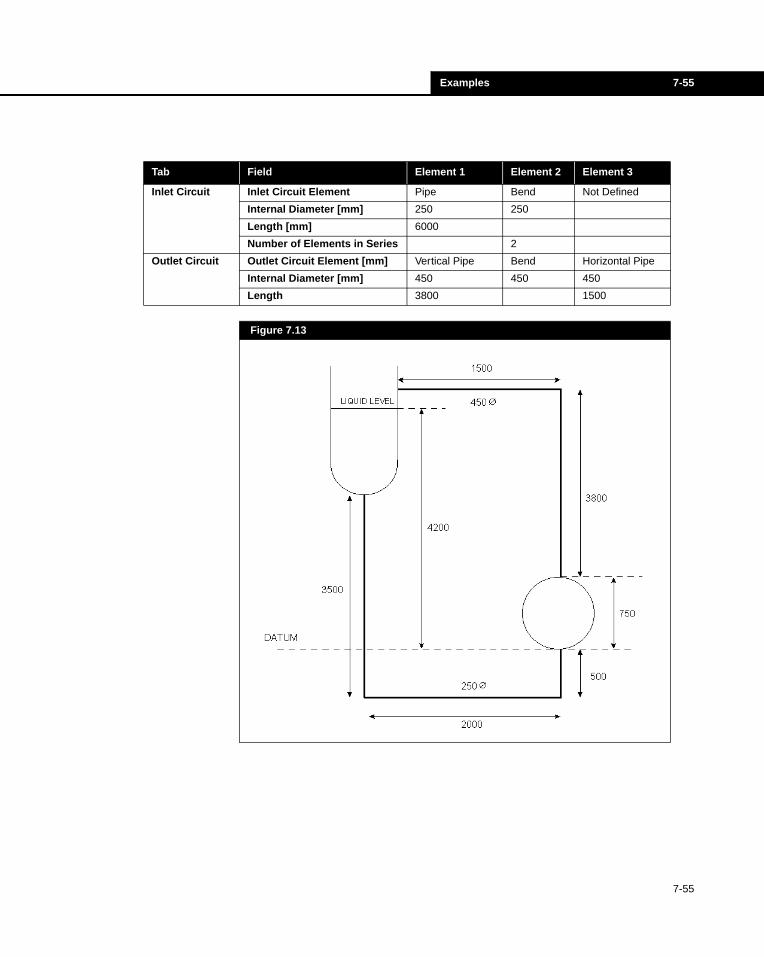
Examples 7-55

Tab Field Element 1 Element 2 Element 3

Inlet Circuit Inlet Circuit Element Pipe Bend Not Defined

Internal Diameter [mm] 250 250

Length [mm] 6000

Number of Elements in Series 2

Outlet Circuit Outlet Circuit Element [mm] Vertical Pipe Bend Horizontal Pipe

Internal Diameter [mm] 450 450 450

Length 3800 1500

Figure 7.13

7-55

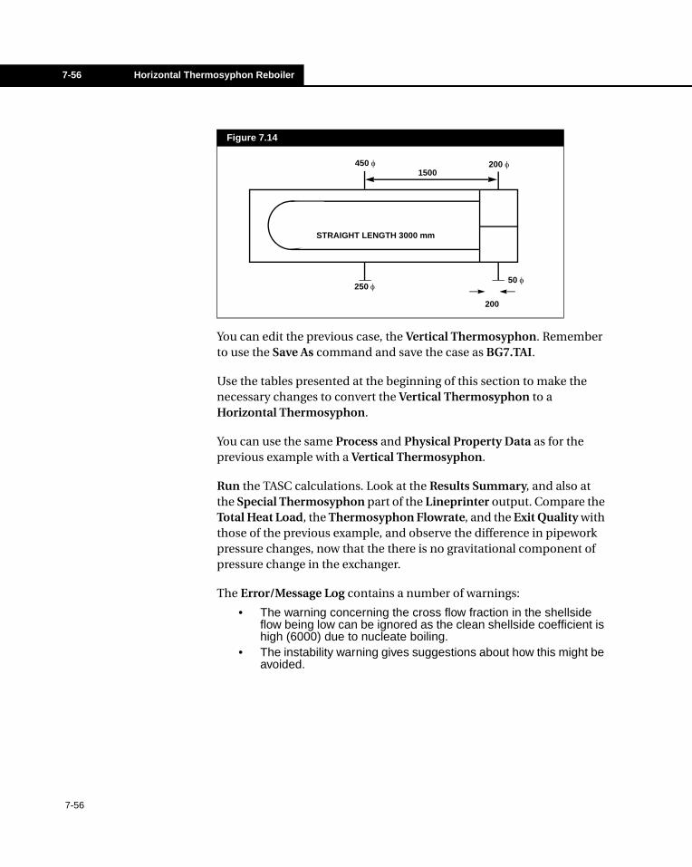
7-56 Horizontal Thermosyphon Reboiler

You can edit the previous case, the Vertical Thermosyphon. Remember to use the Save As command and save the case as BG7.TAI.

Use the tables presented at the beginning of this section to make the necessary changes to convert the Vertical Thermosyphon to a Horizontal Thermosyphon.

You can use the same Process and Physical Property Data as for the previous example with a Vertical Thermosyphon.

Run the TASC calculations. Look at the Results Summary, and also at the Special Thermosyphon part of the Lineprinter output. Compare the Total Heat Load, the Thermosyphon Flowrate, and the Exit Quality with those of the previous example, and observe the difference in pipework pressure changes, now that the there is no gravitational component of pressure change in the exchanger.

The Error/Message Log contains a number of warnings:

• The warning concerning the cross flow fraction in the shellside flow being low can be ignored as the clean shellside coefficient is high (6000) due to nucleate boiling.

• The instability warning gives suggestions about how this might be avoided.

Figure 7.14

450 φ1500

200 φ

250 φ50 φ

200

STRAIGHT LENGTH 3000 mm

7-56

Index

A

Adjustment Factors (costs) 6-7

B

Baffles 1-4Basic Input 2-6, 3-5Bubble Point Temperature 3-8Bundles 1-4

C

Calculation Mode 2-6, 3-5Calculation Type 3-3

Checking (rating) 3-3Design 3-3Simulation 3-3Thermosyphon 3-3

Checking (Rating) 1-3, 2-6Components

Calculation of the Properties of a Mixture 5-14Condenser 7-16Convert Option 3-11Costing Package 6-6

Adjustment Factors 6-7Design Pressure 6-6Labour Costs 6-6Materials Costs 6-6

D

Data Input 3-1Databank 5-13Databanks

Lowfin 6-9Default Input Data File 3-15Default Units 3-10Design 1-3, 2-6Design Mode 3-8Design Pressure 6-6Diagram (Process) 2-5DIPPR 5-19Documentation 1-7

E

Enhanced Surfaces 3-8Equipment Item Number 2-6Error / Warning Message Log 4-8Examples 7-1Exchanger Configuration 3-8Exchanger Geometries

Baffles 1-4Nozzles 1-4Shells/Channels 1-4Tube Bundles 1-4Tubes 1-4

Exchangers in Series 7-35

F

Falling Film Evaporator 7-31Feed Effluent Train 7-37Feedwater Heater 7-4File Extensions 6-10File Structure 6-10File View 4-7Find 1-6, 4-7Find Item 3-13Find Next 4-7Fluid Processes 1-5

G

Geometry 1-4, 3-10Geometry Data Input 3-8

Enhanced Surfaces 3-8Thermosyphon Views 3-8

H

Header 3-8Heat Transfer Coefficients 4-4Help Text 1-8, 2-3, 3-13

Using 3-12HYSYS 5-23

I

Icons 2-8Importing from a Properties Package 5-24Importing from HYSYS 5-23Importing Properties and Process Data 5-20Importing PSF Files 5-20Information Message 3-16Inlet Conditions 3-7Input Directly 5-12Input Errors and Warnings 3-16Input File 3-14

Process block 3-14Properties block 3-14

Input Item Identifier 3-13Input Items

Find Item 3-13

I-1

I-2 Index

I-2

Finding 3-13Main Properties 3-13Physical Properties 3-13

Input Units 3-10Input Views 3-4

Bundle Layout 3-4Enhanced Surfaces 3-4Exchanger Geometry 3-4Nozzles 3-4Options 3-4Physical Properties Data 3-4Process 3-4Thermosyphon Details 3-4Tubes and Baffles 3-4

Introduction 1-1Item Number 3-13

J

Job Title 2-6

K

Kettle Reboiler 7-23

L

Labour Costs 6-6Layout 3-8Line Number 3-13Lineprinter Output 4-6Link units 3-10Lowfin Tube Databank 6-9

M

Mass Flowrate 3-7Materials Costs 6-6Mixture Calculations 5-15Mixture Calculations (Old Style) 5-15

N

NEL40 3-7–3-8, 5-14Nozzles 1-4

O

Other Data Input 3-9Other Facilities 6-1Other Output

Tube Layout Drawing 4-9Outlet Conditions 3-7Outlet Quality 3-7

Outlet Temperature 3-7–3-8Output 1-6, 4-1

Costing Package 4-9Report Generator 4-9Setting Plan 4-9TEMA Specification Sheet 4-9Word Specification Sheet 4-9

Output Files 4-680-column Output 4-6Brief Output 4-6Lineprinter Output 4-6Physical Properties Output 4-6

Output Screens 4-3Alternative Designs 4-3Integration along the Shell 4-3Nozzles 4-3Results Summary 4-3Stream Data 4-3

Output Views 4-3Full Results 4-3

Outside Diameter 4-4Outside Surface 4-4

P

Physical Properties 3-3, 5-1, 5-4Physical Properties (Old Style) 5-4Preferences 3-10Pressure Dependence 5-26Process Constraints View 3-8Process Data 3-8, 3-10Process Data Input 3-7

Bubble Point Temperature 3-8Inlet Conditions 3-7Mass Flowrate 3-7Outlet Conditions 3-7Outlet Quality 3-7Outlet Temperature 3-7–3-8T-h-x (Temperature-enthalpy-quality)

Properties Data 3-7Process Diagram 2-5Process Methods View 3-8Project File Structure 6-10

Output Options 6-10Properties Data 1-5, 3-7–3-8, 3-10Properties Data Input 5-4, 5-11Properties Data Input (Old Style) 5-11Properties Input 5-6Properties Output 5-25Properties Package - Importing 5-24

Index I-3

Properties Used 5-5Property Data

Liquid 5-5T-h-x Data 5-5Vapour 5-5

Property Data Sources 1-5Property Databanks 5-18

DIPPR 5-19NEL40 5-19

PSF Files 5-20

R

Reboiler 7-23, 7-45, 7-54Resistances 4-4Results Summary 2-7, 4-7Run Progress 2-7Run Title 2-5Running TASC 2-7

S

Setting Plan 1-3, 6-3DXF file 6-4TEMA Output Sheet 6-4

Shell 3-8Shell Types 1-4Simulation 1-3, 2-6, 4-4Single Component Stream from NEL40 5-14Start up 2-5–2-6

Equipment Item Number 2-6Job Title 2-6

Starting TASC 2-4Stream Pressure Drops 4-4Surface Area Ratio 4-4

T

TASC Icons 2-8TEMA 3-8TEMA Input 3-6

Exchanger General Form 3-6Shellside 3-6TEMA sheet 3-6Tubeside 3-6

TEMA Output Sheet 6-4Thermal Design Calculation 6-4Thermosyphon 1-3, 1-6, 2-6, 7-45, 7-54Thermosyphon Mode 4-4Thermosyphon Views 3-8Tube Bundles 1-4Tube Layout 3-17

Tube Size 3-8Tubes 1-4Twisted Tape 1-4

U

Units 3-10User Databank 5-13Using Help 3-12Using TASC 2-1

V

Vapour Shear 1-5View 2-5

W

Word Specification Sheet 6-8

I-3

I-4 Index

I-4