Aspen Plus 2004 - University of Alberta · Introducing Aspen Plus 8 Introducing Aspen Plus Aspen...
114
Aspen Engineering Suite 2004.1 Aspen Plus 2004.1 Getting Started: Building and Running a Process Model
Transcript of Aspen Plus 2004 - University of Alberta · Introducing Aspen Plus 8 Introducing Aspen Plus Aspen...

Build
Aspen Engineering Suite 2004.1
Aspen Plus 2004.1 Getting Started:
ing and Running a Process Model

Who Should Read this Guide 2
Who Should Read this Guide
This guide is suitable for beginners to the Aspen Plus simulation environment. Users should understand the material in this guide before proceeding to the other Aspen Plus Getting Started Guides.

Contents 3
Contents
INTRODUCING ASPEN PLUS ............................................................................ 8 Why Use Process Simulation? .................................................................................... 8 What is an Aspen Plus Process Simulation Model? ......................................................... 8 Sessions in this Book................................................................................................ 9 Using Backup Files ................................................................................................. 10
1 ASPEN PLUS BASICS................................................................................... 11 Starting Aspen Plus ................................................................................................ 11 The Aspen Plus Main Window................................................................................... 11 Opening a File ....................................................................................................... 12
To Display the File Menu .................................................................................... 12 Selecting Flowsheet Objects .................................................................................... 15 Using a Shortcut Menu............................................................................................ 16
To Display the Shortcut Menu for Stream 1........................................................... 16 Opening Input Sheets............................................................................................. 17
To Open the Input Sheets for Stream 1 ................................................................ 17 Using Help ............................................................................................................ 19
To Get Help on any Topic ................................................................................... 20 Entering Data on a Sheet ........................................................................................ 21 Expert Guidance � the Next Function ........................................................................ 22
To Use the Next Function to Display the Next Required Sheet .................................. 22 Running the Simulation...................................................................................... 25 To Run the Simulation ....................................................................................... 25
Examining Stream and Block Results ........................................................................ 26 To Display the Flash Overhead Vapor (Stream 2) Results ........................................ 26
Modifying and Rerunning Your Model ........................................................................ 28 Saving Your File and Exiting Aspen Plus..................................................................... 28
To Change the Save Options............................................................................... 28 To Save and Exit............................................................................................... 30
2 BUILDING AND RUNNING A PROCESS SIMULATION MODEL...................... 31 Building the Process Model ...................................................................................... 31 Defining the Simulation: Methylcyclohexane Recovery Column ..................................... 32

Contents 4
Starting Aspen Plus ................................................................................................ 33 Creating a New Simulation ...................................................................................... 33
To Specify the Application Type and Run Type for the New Run ............................... 33 The Aspen Plus Main Window................................................................................... 34 Defining the Flowsheet............................................................................................ 34
To Select a Unit Operation Block ......................................................................... 34 To Choose a RadFrac Icon and Place a Block ......................................................... 35 To Connect Streams to the Block......................................................................... 36
Adding Data to the Process Model............................................................................. 37 Specifying a Title for the Simulation.......................................................................... 37 Specifying Data to be Reported ................................................................................ 39 Entering Components ............................................................................................. 40
To Enter a Unique Component ID for Each Component ........................................... 40 Selecting Thermodynamic Methods........................................................................... 42
To Find the Appropriate Type of Base Method for this Simulation.............................. 43 Entering Stream Data ............................................................................................. 44 Entering Unit Operation Block Data........................................................................... 46 Running the Simulation........................................................................................... 49 Examining Simulation Results .................................................................................. 50
To Display the Results for Block B1...................................................................... 50 Examining Stream Results....................................................................................... 53
To Display the Results for Stream 3 ..................................................................... 53 To Display the Results for All Streams on the Same Sheet....................................... 54
Changing Input Specifications .................................................................................. 54 To Increase the Phenol Solvent Stream Flow Rate.................................................. 54
Rerunning the Simulation with Changed Input............................................................ 55 Creating Reports.................................................................................................... 55
To Generate a Report File................................................................................... 55 To View and Save Part of a Report....................................................................... 56
Saving Your File and Exiting Aspen Plus..................................................................... 57
3 PERFORMING A SENSITIVITY ANALYSIS................................................... 58 Starting Aspen Plus ................................................................................................ 58 Opening an Existing Simulation ................................................................................ 59
If Your Saved File MCH.apw is Displayed .............................................................. 59 If Your Saved File MCH.apw is not Displayed ......................................................... 59
Saving a Simulation under a New Name .................................................................... 60 Defining the Sensitivity Analysis................................................................................ 60

Contents 5
Entering Sensitivity Specifications ............................................................................ 60 To Create a New Sensitivity Block........................................................................ 60 To Define XMCH as Distillate Product Purity........................................................... 61 To Define QCOND as the Condenser Duty and QREB as Reboiler Duty....................... 62 To Specify the Manipulated Variable..................................................................... 64 To Format the Tabular Results ............................................................................ 66
Running the Sensitivity Analysis................................................................................ 67 Displaying Sensitivity Analysis Results ...................................................................... 68 Plotting Sensitivity Results ...................................................................................... 69
To Generate a Plot of MCH Distillate Purity Versus Phenol Flow Rate ......................... 69 Saving Your File and Exiting Aspen Plus..................................................................... 70
4 MEETING PROCESS DESIGN SPECIFICATIONS .......................................... 71 Starting Aspen Plus ................................................................................................ 71 Opening an Existing Simulation ................................................................................ 71
If Your Saved MCHSENS.apw is Displayed............................................................. 71 If Your Saved File MCHSENS.apw is Not Displayed ................................................. 72
Saving a Simulation Under a New Name..................................................................... 72 Defining the Design Specification .............................................................................. 73
To Enter Design Specifications ............................................................................ 73 To Define XMCH in DS-1 .................................................................................... 74 To Set Up the Design Specification ...................................................................... 74 To Specify the Manipulated Variable..................................................................... 75
Running the Design Specification Analysis ................................................................. 76 Examining Design Specification Results ..................................................................... 77 Exiting Aspen Plus.................................................................................................. 77
5 CREATING A PROCESS FLOW DIAGRAM..................................................... 78 Starting Aspen Plus ................................................................................................ 78 Opening an Existing Simulation ................................................................................ 79
If Your Saved File MCH.apw is Displayed .............................................................. 79 If Your Saved File MCH.apw is not Displayed ......................................................... 79
Switching to PFD Mode ........................................................................................... 80 Adding a Pump to the Diagram ................................................................................ 80
To Add the Feed Pump to the PFD Diagram........................................................... 81 To Insert the Pump Into the Feed Stream............................................................. 81
Displaying Stream Data .......................................................................................... 83 To Display Temperature and Pressure .................................................................. 83
Adding a Stream Table ........................................................................................... 84

Contents 6
To Zoom in on Part of the Diagram ...................................................................... 85 Adding Text .......................................................................................................... 85
To Display the Draw Toolbar ............................................................................... 85 To Add Text ..................................................................................................... 85
Printing a Process Flow Diagram............................................................................... 86 To Preview Your Drawing Before Printing .............................................................. 86 To Print the PFD-Style Drawing ........................................................................... 86
Leaving PFD Mode.................................................................................................. 87 To Return to Simulation Mode ............................................................................. 87
Exiting Aspen Plus.................................................................................................. 87
6 ESTIMATING PHYSICAL PROPERTIES FOR A NON-DATABANK COMPONENT88 Thiazole Physical Property Data................................................................................ 88 Starting Aspen Plus ................................................................................................ 89 Creating a Property Estimation Simulation ................................................................. 89 Entering a Title ...................................................................................................... 90 Entering Components Information ............................................................................ 90 Specifying Properties to Estimate ............................................................................. 92 Entering Molecular Structure.................................................................................... 93
To Enter the Molecular Structure Information for Thiazole ....................................... 93 Entering Property Data ........................................................................................... 95
To Enter Pure Component Boiling Point and Molecular Weight for Thiazole ................. 95 To Enter Antoine Vapor Pressure Correlation Coefficients ........................................ 96
Running a Property Constant Estimation (PCES) ......................................................... 98 Examining Property Constant Estimation Results ........................................................ 99
To Examine PCES Results ................................................................................... 99 Creating and Using a Property Backup File ................................................................100
To Save a Backup File.......................................................................................100 To Import a Backup File ....................................................................................101
Exiting Aspen Plus.................................................................................................102
7 ANALYZING PROPERTIES .........................................................................103 Starting Aspen Plus ...............................................................................................103 Entering Components and Properties .......................................................................104 Generating a Txy Diagram......................................................................................106
To Generate a Txy Diagram ...............................................................................107 To Generate an Activity Coefficient Plot ...............................................................108

Contents 7
8 CONNECTING TO THE ASPEN PLUS SIMULATION ENGINE ........................110
9 GENERAL INFORMATION..........................................................................111 Copyright.............................................................................................................111 Related Documentation..........................................................................................112
TECHNICAL SUPPORT...................................................................................113 Online Technical Support Center .............................................................................113 Phone and E-mail..................................................................................................114

Introducing Aspen Plus 8
Introducing Aspen Plus
Aspen Plus makes it easy to build and run a process simulation model by providing you with a comprehensive system of online prompts, hypertext help, and expert system guidance at every step. In many cases, you will be able to develop an Aspen Plus process simulation model without referring to printed manuals.
The seven hands-on sessions show you, step-by-step, how to use the full power and scope of Aspen Plus. Each session requires 30 � 50 minutes.
This guide assumes only that you have an installed copy of Aspen Plus. If you have not installed Aspen Plus, please see the Aspen Engineering Suite installation manual.
Why Use Process Simulation? Process simulation allows you to predict the behavior of a process by using basic engineering relationships, such as mass and energy balances, and phase and chemical equilibrium. Given reliable thermodynamic data, realistic operating conditions, and rigorous equipment models, you can simulate actual plant behavior. Process simulation enables you to run many cases, conduct "what if" analyses, and perform sensitivity studies and optimization runs. With simulation, you can design better plants and increase profitability in existing plants.
Process simulation is useful throughout the entire lifecycle of a process, from research and development through process design to production.
What is an Aspen Plus Process Simulation Model? A process consists of chemical components being mixed, separated, heated, cooled, and converted by unit operations. These components are transferred from unit to unit through process streams.
You can translate a process into an Aspen Plus process simulation model by performing the following steps:
1 Define the process flowsheet:
− Define the unit operations in the process.

Introducing Aspen Plus 9
− Define the process streams that flow to and from the unit operations. − Select models from the Aspen Plus Model Library to describe each unit
operation and place them on the process flowsheet. − Place labeled streams on the process flowsheet and connect them to
the unit operation models.
2 Specify the chemical components in the process. You can take these components from the Aspen Plus databanks, or you can define them.
3 Specify thermodynamic models to represent the physical properties of the components and mixtures in the process. These models are built into Aspen Plus.
4 Specify the component flow rates and the thermodynamic conditions (for example, temperature and pressure) of feed streams.
5 Specify the operating conditions for the unit operation models.
With Aspen Plus you can interactively change specifications such as, flowsheet configuration; operating conditions; and feed compositions, to run new cases and analyze process alternatives.
In addition to process simulation, Aspen Plus allows you to perform a wide range of other tasks such as estimating and regressing physical properties, generating custom graphical and tabular output results, fitting plant data to simulation models, optimizing your process, and interfacing results to spreadsheets.
Sessions in this Book The hands-on sessions in this book are described in the following table:
Follow the steps in this chapter
To Learn how to
1 Aspen Plus Basics Start Aspen Plus, use the Aspen Plus user interface, and exit Aspen Plus.
2 Building and Running a Process Simulation Model
Build and run a typical Aspen Plus process simulation model.
3 Performing a Sensitivity Analysis
Use Aspen Plus to study the sensitivity of process performance to changes in process feeds and operating variables.
4 Meeting Process Design Specifications
Use Aspen Plus to make your process model meet a design specification by manipulating a process feed or operating variable.
5 Creating a Process Flow Diagram
Add stream tables, graphics, and text to your process flowsheet.
6 Estimating Physical Properties for a Non-Databank Component
Use Aspen Plus to enter and estimate missing physical properties required for simulation.
7 Analyzing Properties Use Aspen Plus to generate tables and plots of physical properties, computed over a range of values.

Introducing Aspen Plus 10
Using Backup Files We recommend that you perform all sessions sequentially using the results of the previous chapter in the current chapter. However, you can skip chapters and work on the session of your choice using backup files containing simulation data.
Aspen Plus provides backup files (filename.bkp) containing all problem specifications and results for each tutorial session. In some cases, if you skip a session, you need to load a backup file to supply missing data. Each chapter contains instructions for how to do this.

1 Aspen Plus Basics 11
1 Aspen Plus Basics
This chapter leads you through an Aspen Plus simulation to explain how to open a file, enter data, run a simulation, and examine results.
Allow about 30 minutes for this session.
Starting Aspen Plus 1 From your desktop, select Start and then select Programs.
2 Select AspenTech, then Aspen Engineering Suite, then Aspen Plus 2004.1, and then Aspen Plus User Interface.
The Aspen Plus Startup dialog box appears. Aspen Plus displays a dialog box whenever you must enter information or make a selection before proceeding.
3 Select Blank Simulation, then click OK.
If the Connect to Engine dialog box appears, see Chapter 8.
Note: To create a Windows desktop icon for Aspen Plus, navigate to the xeq folder of the Aspen Plus User Interface installation. Then, select the apwn.exe program and drag it onto your Windows desktop. Double-click the icon to start Aspen Plus.
The Aspen Plus Main Window The Aspen Plus main window (shown below) appears when you start Aspen Plus. From the menu bar, select Window and then select Workbook to get the display style shown below. Workbook mode is used in all the examples in this book.
The Process Flowsheet Window appears automatically along with the Aspen Plus menu bar, various toolbars, and the Model Library.
Aspen Plus displays context-dependent definitions and information in the prompt area of the main window. Whenever you need information about the currently highlighted item, refer to the prompt area for guidance.

1 Aspen Plus Basics 12
Help Button Next Button
Menu Bar
Toolbars
Process Flowsheet
Select Mode button
Model Library
Prompt area
Opening a File Open a file for an Aspen Plus simulation by either:
1 Double-clicking the file in Windows.
2 Selecting the Open command from the File menu in Aspen Plus.
In this section, use the Open command on the File menu to open a partially completed Aspen Plus simulation stored in a backup file.
To Display the File Menu 1 From the menu bar, select File.
The File menu appears:

1 Aspen Plus Basics 13
2 From the File menu, select Open.
The Open dialog box appears. Your default working directory appears in the Look in list.
3 Click .
A list of folders appears in the Open dialog box:

1 Aspen Plus Basics 14
By default, the Favorites list contains five folders that are provided with Aspen Plus. The files in these folders are designed to assist in creating suitable simulation models in Aspen Plus.
Note: Add folders to the Favorites list by navigating to the
appropriate folder and clicking .
4 Double-click the Examples folder.
5 From the files list, select flash.bkp and click Open.
6 From the Aspen Plus dialog box, click Yes to close the current run before opening a new run.
7 If Aspen Plus prompts "Save changes to Simulation 1?", click No.
While Aspen Plus opens the simulation model, the cursor shows the busy symbol, to indicate that Aspen Plus is finishing an operation. When the operation is complete, the cursor returns to the arrow shape.
Note: You don�t have to close the current run before opening a new run. If you click No in step 6, you will have two Aspen Plus applications running at the same time, each with one open simulation (Aspen Plus cannot open multiple simulations).

1 Aspen Plus Basics 15
Selecting Flowsheet Objects Aspen Plus displays the process flowsheet for the opened Flash simulation:
Process flowsheets display streams and unit operation blocks. The Flash simulation has one feed stream (stream 1), two product streams (streams 2 and 3), and one unit operation block (B1).
Next, select the feed stream (stream 1) on the process flowsheet and enter specifications.

1 Aspen Plus Basics 16
Using a Shortcut Menu A shortcut menu of commands is available for the flowsheet objects.
To Display the Shortcut Menu for Stream 1 1 Select Stream 1 and click the right mouse button.
Note: Make sure the tip of the cursor arrow is touching the stream, otherwise you will get the flowsheet shortcut menu instead of the stream shortcut menu.
The stream shortcut menu appears, listing the executable commands for stream 1:

1 Aspen Plus Basics 17
2 Use the Up and Down arrow keys on your keyboard, to highlight the commands in the shortcut menu.
The prompts at the bottom of the main window change as you highlight each command.
Opening Input Sheets Aspen Plus provides input sheets to allow you to specify the components of a stream and properties such as temperature. There are a number of ways to access the input sheets:
• From the Aspen Plus menu bar, select Data and then select Data Browser, then use the Data Browser menu tree to navigate to the Streams | 1 | Input | Specifications sheet.
Note: The item | sub-item shorthand means �click item then click sub-item.� This shorthand will be used for many hierarchical selection processes including menus.
• From the Aspen Plus menu bar, select Data and then select Streams.
• Click the streams button in the Data Browser toolbar, then use the Data Browser menu tree to navigate to the Streams | 1 | Input | Specifications sheet.
• From the stream 1 shortcut menu, select Input.
To Open the Input Sheets for Stream 1 1 From the process flowsheet, select Stream 1, then click the right mouse
button.
2 From the stream shortcut menu, select Input.
Tip: To open a stream or block input sheet quickly, double-click the object from the process flowsheet.

1 Aspen Plus Basics 18
The Stream 1 Input Specifications sheet appears with the Data Browser menu tree in the left pane:
Data Browser Menu Tree
Window Tabs
Navigate from sheet to sheet by expanding the folders in the Data Browser menu tree and clicking the lowest level objects. For example, if you want to see the input sheet for Block B1, expand the Blocks folder and the B1 folder and click Input.
Navigate from window to window by clicking the Window Tabs. For example, if you want to go back to the Process Flowsheet, click its tab.

1 Aspen Plus Basics 19
Using Help Before specifying the characteristics of Stream 1 you may wish to get context-sensitive help about the sheet itself, the form to which it belongs, or about the various fields within the sheet. There are a number of ways to do this:
• Click , then click the box or sheet.
-or-
• From the Aspen Plus menu bar, click Help, select What�s This?, then click the box or sheet.
-or-
• Click the box or sheet, then press F1 (the help key).
Get help on the Stream 1 Input Specifications sheet and on the whole input form.
1 Click .
2 Click the tab labeled Specifications.
Aspen Plus displays a help window that explains how to use the Stream Input Specifications sheet:
If you click the Stream Input Form link at the bottom of this help window, Aspen Plus displays a the help for the Stream Input form, which, in this case, consists of five sheets: Specifications, Flash Options, PSD, Component Attr., and EO Options.

1 Aspen Plus Basics 20
Note: A sheet may be required, unavailable, or optional. In this example, the Specifications sheet is required and incomplete
(hence the symbol: ). The PSD and Component Attr. sheets are unavailable. The Flash Options and EO Options sheets are optional.
3 Scroll to the end of the help topic and click the green underlined text Stream Input Form.
The Stream Input Form help topic appears.
4 When finished, click to close the help window.
To Get Help on any Topic You can get help on any topic at any time by using the Help menu.
1 From the Aspen Plus menu bar, select Help.
2 Use the Up and Down arrow keys on the keyboard to move through the Help menu.
3 Read the descriptions for each item at the bottom left corner of the screen.
4 From the Help menu, select Help Topics.
5 In the Contents pane at the left, double-click Using Aspen Plus Help.
Tip: You can click the Help Topics button in the help window's toolbar to hide or reveal the left pane which displays the Contents, Index, and Search tabs. You can click the Index and Search tabs to look for help by subject.
6 Double-click a topic labeled with the icon to display the associated help window or double-click items labeled with the icon to view more topics.
7 When finished, click to close the help window.

1 Aspen Plus Basics 21
Entering Data on a Sheet Once an input sheet is open, state variables, units, and numeric data may be entered into the available fields (white rectangular boxes) or selected from drop-down lists. There are two ways to move from field to field on a sheet:
• Press the Tab key on your keyboard.
• Position the cursor in the field and left-click.
In this simulation, enter missing temperature, pressure, and component flow data for Stream 1.
1 If necessary click in the Stream 1 Input Specifications sheet to make it active.
2 Enter the following state variable and component flow specifications:
Parameter Value Units
Temperature 180 F
Pressure 20 psi
Methanol mole-flow 50 lbmol/hr
Water mole-flow 50 lbmol/hr
Since the default units are appropriate for this simulation, you only need to enter the values.
The completed Stream 1 Input Specifications sheet appears below (the Data Browser menu tree is not shown):
When all required specifications have been entered, a check mark ( ) appears on the tab containing the sheet name. Check marks also appear in the Data Browser menu tree.

1 Aspen Plus Basics 22
Expert Guidance � the Next Function The Aspen Plus expert system, known as the Next function, guides you through all the steps for entering specifications for your simulation model. The Next function:
• Guides you through the required and optional input for a simulation by displaying the appropriate sheets.
• Displays messages informing you what you need to do next.
• Ensures that you do not enter incomplete or inconsistent specifications even when you change options and specifications you have already entered.
To Use the Next Function to Display the Next Required Sheet 1 From the Data Browser, click .
Note: The button can also be found in the Data Browser toolbar of the main window.
Aspen Plus displays the next sheet that requires input data, in this case, the Blocks | B1 | Input | Specifications sheet:
Now you should enter the temperature and pressure specifications.
If you click while the sheet is incomplete, the Completion Status dialog box appears indicating the missing specifications:

1 Aspen Plus Basics 23
Click to close the Completion Status message box.
2 Change the first field in the Flash specifications area from Temperature
to Heat Duty by clicking and selecting Heat Duty from the list.
3 In the Heat Duty value field, type 0. There is no need to change the units (Btu/hr is the default).
4 Make sure the first field in the second line of the Flash specifications area reads Pressure, then type 1 in the Pressure value field.
5 In the Pressure units field, click and select atm to change the input units from psi to atm.
6 The box in the Valid phases area is set to Vapor-Liquid by default. For this simulation, accept the default.
Note: Default options on Data Browser sheets appear shaded unless you modify them, in which case they will appear in black text.
The input data on the Block B1 Input Specifications sheet is now complete:

1 Aspen Plus Basics 24
The checkmarks in the Data Browser menu tree and the absence of partially filled circles indicates that all required data have been entered. The Input Complete message in the lower left corner of the Data Browser window confirms that Block B1 is fully specified and the Required Input Complete message in the lower right corner of the main window confirms that all blocks and streams are ready for a simulation run.
Note: The Data Browser window is on top of the process flowsheet window. To look at your process flowsheet, click its tab. Alternatively, click Windows from the Aspen Plus menu bar, and select Process Flowsheet Window.

1 Aspen Plus Basics 25
Running the Simulation The input specifications for this simulation model are complete and the simulation is ready to be run. Run the simulation in any of the following ways:
• From the Aspen Plus menu bar, select Run, and then select Run.
• From the Aspen Plus toolbar, click .
• Click to open the Control Panel and then click from the Control Panel.
• Press F5.
Once the process flowsheet has been fully specified, running the simulation is easy.
To Run the Simulation 1 From the Aspen Plus menu bar, click Run.
The Run menu appears:
2 From the Run menu, select Run.
While Aspen Plus performs calculations for the simulation, the cursor has a stop sign shape. The block being executed is also highlighted in the process flowsheet window. When the calculations are complete, the cursor returns to the arrow shape. In the status bar at the bottom of the main window, the prompt message Simulation run completed appears on the left, and on the right, the status message Results Available appears in blue.

1 Aspen Plus Basics 26
Note: If the calculations are completed with errors or warnings, the status message indicates Results Available with Errors and Results Available with Warnings, respectively.
Examining Stream and Block Results Now view the results for the flash overhead vapor stream (Stream 2) and for the flash block (Block B1).
To Display the Flash Overhead Vapor (Stream 2) Results 1 Display the process flowsheet by clicking its tab.
Note: If the streams in your process flowsheet now have temperature and pressure data attached to them, you can remove these attachments by clicking View and selecting Global Data. Or, you may wish to click View, select Zoom, and then select Zoom Out or Zoom Full to make your flowsheet look nice with the attachments.
2 Select stream 2 and right-click on the stream to display the shortcut menu.
3 From the shortcut menu, select Results.
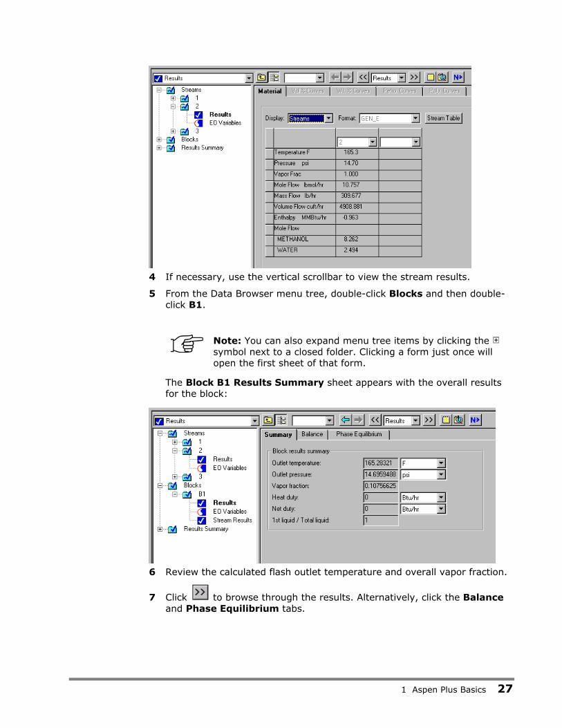
The Data Browser window opens with the Streams | 2 | Results | Material sheet in view, providing the thermodynamic state and composition flows of the vapor stream:
1 Aspen Plus Basics 27
4 If necessary, use the vertical scrollbar to view the stream results.
5 From the Data Browser menu tree, double-click Blocks and then double-click B1.
Note: You can also expand menu tree items by clicking the symbol next to a closed folder. Clicking a form just once will open the first sheet of that form.
The Block B1 Results Summary sheet appears with the overall results for the block:
6 Review the calculated flash outlet temperature and overall vapor fraction.
7 Click to browse through the results. Alternatively, click the Balance and Phase Equilibrium tabs.

1 Aspen Plus Basics 28
Modifying and Rerunning Your Model 1 From the process flowsheet, select and right-click Stream 1 to display the
stream shortcut menu.
2 Select Input.
The Data Browser window opens with the Streams | 1 | Input | Specifications sheet in view.
3 In the Composition area, enter the following values for the component mole-flows:
Component Value
Methanol 60
Water 40
4 From the Aspen Plus menu bar, click Run, then select Run to run the simulation with the new feed stream values.
5 When the run is completed, display the new results for the outlet streams and the flash block.
Saving Your File and Exiting Aspen Plus For this example, save your file as both an Aspen Plus document (.apw) file and an Aspen Plus backup (.bkp) file. Document files contain all the intermediate convergence information from the simulation and are useful for saving long simulations. Document files are not forward compatible for new versions of Aspen Plus.
Backup files are compact, portable, and are forward compatible but contain only the input specifications and simulation results. The first run using a backup file will take just as long as the very first run of the simulation.
First, set Aspen Plus to create a backup file with each save.
To Change the Save Options 1 From the Aspen Plus menu bar, select Tools and then select Options.
The Options dialog box appears:

1 Aspen Plus Basics 29
2 On the General tab, in the Save options area, select the checkbox next to Always create backup copy, if it is not already checked.
3 Make sure Aspen Plus documents (*.apw) appears in the Save documents as field.
4 Click OK.
Next, save the simulation and exit Aspen Plus.

1 Aspen Plus Basics 30
To Save and Exit 1 From the Aspen Plus menu bar, select File and then select Save As.
The Save As dialog box appears:
2 If necessary, use the Save in list to navigate to your Aspen Plus working
folder. In this example, the folder is located in D:\Program Files\AspenTech\Working Folders\Aspen Plus 2004.1.
3 Click Save.
Aspen Plus will place a file called Flash.apw and a file called Flash.bkp in your Aspen Plus working folder. See the Aspen Plus User Guide for detailed descriptions of the characteristics of these files.
4 From the Aspen Plus menu bar, click File and select Exit.
You have completed an Aspen Plus simulation.

2 Building and Running a Process Simulation Model 31
2 Building and Running a Process Simulation Model
In this simulation, create an Aspen Plus process model for a methylcyclohexane (MCH) recovery column.
This simulation is divided into three sections:
1 Building the Process Model
2 Adding Data to the Process Model
3 Running the Simulation
Allow about 50 minutes for this simulation.
Building the Process Model In this section, build the process model by performing these tasks:
1 Define the process to be simulated.
2 Start Aspen Plus.
3 Create a new simulation.
4 Build a process flowsheet.

2 Building and Running a Process Simulation Model 32
Defining the Simulation: Methylcyclohexane Recovery Column The process flow diagram and operating conditions are shown in Figure 2.1.
Figure 2.1 Simulation Definition: MCH Recovery Column
MCH and toluene form a close-boiling system that is difficult to separate by simple binary distillation. In the recovery column in Figure 3.1, phenol is used to extract toluene, allowing relatively pure methylcyclohexane to be recovered in the overhead.
The purity of the recovered methylcylohexane depends on the phenol input flow rate. In this session, create an Aspen Plus simulation that allows you to investigate the performance of the column.

2 Building and Running a Process Simulation Model 33
Starting Aspen Plus 1 From your desktop, select Start and then select Programs.
2 Select AspenTech, then Aspen Engineering Suite, then Aspen Plus 2004.1, then Aspen Plus User Interface.
The Aspen Plus Startup dialog box appears. Create a new simulation using an Aspen Plus built-in template.
Creating a New Simulation Aspen Plus provides built-in templates for applications such as chemicals, petroleum, electrolytes, specialty chemicals, pharmaceuticals, and metallurgy.
1 In the Aspen Plus Startup dialog box, select Template and click OK.
The New dialog box appears.
Use the New dialog box to specify the Application Type and the Run Type for the new run. Aspen Plus uses the Application Type you choose to automatically set various defaults appropriate to your application.
To Specify the Application Type and Run Type for the New Run 2 Select the General with English Units template.
The default Run Type, Flowsheet, is appropriate for this simulation.
3 Click OK to apply these options.
2 Building and Running a Process Simulation Model 34
It takes a few seconds for Aspen Plus to finish setting up the new problem.
Note: If the Connect to Engine dialog box appears, see Chapter 8.
The Aspen Plus main window is now active.
The Aspen Plus Main Window The main window appears when you start Aspen Plus. Because you have not entered any simulation specifications yet, the workspace is blank.
For more information about this window, refer to the section The Aspen Plus Main Window in Chapter 1.
Defining the Flowsheet In the flowsheet for the MCH process shown in Figure 2.1, there are two feed streams (MCH-toluene feed and phenol solvent), one unit operation (an extractive distillation column), and two product streams (distillate and bottoms).
Set up the Aspen Plus process flowsheet by placing the unit operation block in the workspace and connecting four streams to it.
Note: If you click before building the process flowsheet, Aspen Plus displays the Flowsheet Definition dialog box, informing you that the first step is to build the process flowsheet. Click OK and build the flowsheet.
To Select a Unit Operation Block 1 From the Model Library at the bottom of the Aspen Plus Process Flowsheet
Window, select the Columns tab.
The list of available distillation columns appears displayed as a row of icons. Moving the cursor over a block causes a description to appear in the lower left of the window.
2 Read the prompt for the RadFrac block.
The description suggests this is the right model for this simulation.
3 Select RadFrac, then press F1 (the Help key) on the keyboard.
The help information confirms that RadFrac is suitable for extractive distillation.

2 Building and Running a Process Simulation Model 35
4 Click at the top of the Help window to close it.
A number of icons are available to represent the RadFrac block.
To Choose a RadFrac Icon and Place a Block 1 Click the arrow to the right of the RadFrac column.
The available icons for RadFrac appear:
2 Move the cursor over the displayed icons to view the label for each icon.
3 Select the icon labeled FRACT1 and drag it (click and hold) into your process flowsheet. This will allow you to place a single block onto your process flowsheet.
4 Move the mouse to the middle of the workspace and release the mouse button.
The block appears on the flowsheet with the default name B1:
Notes about block placement:
• FRACT1 is now the default icon for the RadFrac block.
• Clicking once on an icon enables multiple block placement. The cursor becomes a crosshair and you can click anywhere on the process flowsheet
to place any number of blocks. Click when finished.
• To stop the automatic naming of blocks, select Tools, then Options, then the Flowsheet tab and then clear the appropriate checkbox.
• Your RadFrac block may have a 3-D appearance. The 3D icon option on the Tools | Options | Styles tab determines whether these icons are used.

2 Building and Running a Process Simulation Model 36
To Connect Streams to the Block
1 From the Model Library, click once. This will allow you to place multiple streams.
2 Move the cursor (now a crosshair) onto the process flowsheet.
Ports on the block that are compatible with the stream are indicated by arrows. Red means required; blue means optional. Hover over a port to see a description.
3 Find the Feed (Required; one or more) port and click once to connect a feed stream to the port.
4 Move the cursor to any blank part of the process flowsheet and click once to begin the feed stream (named Stream 1 by default) at that location.
5 Create another material feed stream (named Stream 2 automatically) connecting to block B1 at the same port as Stream 1 by repeating steps 3 and 4.
6 Create another stream (Stream 3) connected to the liquid distillate port near the top of the block. The full name of this port is: Liquid Distillate (Required if Distillate Vapor Fraction < 1(Setup Condenser sheet)).
7 Connect Stream 4 to the Bottoms (Required) port.
8 Click to stop adding streams.
Your process flowsheet is now complete:
The status indicator in the bottom right of the main window says Required Input Incomplete indicating that further input specifications are required before running the simulation.
2 Building and Running a Process Simulation Model 37
Notes about Stream placement:
• To select a Heat or Work stream instead of a Material stream, click the arrow next to the stream button and choose either the Heat or Work stream icon.
• To cancel connecting a stream at any time, press the Escape key.
• You can delete a stream by selecting it and pressing the Delete key. However, Aspen Plus will continue to increment the numeric label for new streams, if they are being labeled automatically.
• To rename a particular stream, select it, right-click, and select Rename Stream on the shortcut menu.
• The easiest way to get the shortcut menu is to select the stream label and right-click in its box.
• Click the stream icon in the Model Library and drag to place a single stream. Drag to a port and release the mouse button to connect the stream. Move the cursor to any blank area or another port and click once to place the other end of the stream.
Adding Data to the Process Model Now that you have created your process flowsheet, use the Data Browser input sheets to enter the remaining required information for this run.
The Aspen Plus Next function displays the required input sheets automatically. You can also navigate to an input sheet in any of the following ways:
• Click Data in the Aspen Plus menu bar and select the sheet you want.
• Click Data on the Aspen Plus menu bar, select Data Browser, and use the menu tree to navigate to any input sheet.
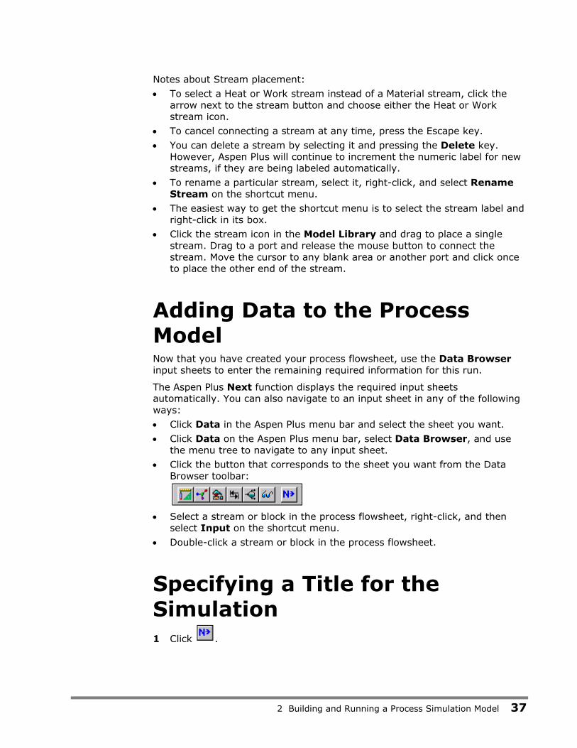
• Click the button that corresponds to the sheet you want from the Data Browser toolbar:
• Select a stream or block in the process flowsheet, right-click, and then
select Input on the shortcut menu.
• Double-click a stream or block in the process flowsheet.
Specifying a Title for the Simulation 1 Click .

2 Building and Running a Process Simulation Model 38
Aspen Plus displays the Flowsheet Complete dialog box indicating that your flowsheet is complete and that you need to provide remaining specifications.
2 Click OK to display the first required input sheet.
Aspen Plus opens the Data Browser window containing the Data Browser menu tree and the Setup | Specifications | Global sheet:
3 In the Title box, enter the text Methylcyclohexane Recovery Process and press Enter on the keyboard.
The Setup | Specifications | Global sheet displays a number of settings that apply to the whole simulation. The chosen template set the units to English (ENG). These may be changed here globally, or in other sheets for particular streams or blocks. For more information about global specifications see the Aspen Plus User Guide, Chapter 5: Global Information for Calculations.

2 Building and Running a Process Simulation Model 39
Specifying Data to be Reported Results data may be examined interactively in Aspen Plus or after exiting by viewing a report file with a text editor.
For this simulation, tell Aspen Plus to calculate mole fractions as well as a built-in set of properties called TXPORT.
1 Navigate to the Setup | Report Options form by clicking once on the Report Options form under the Setup folder in the Data Browser menu tree.
Note: If the Report Options form is not visible click the symbol next to the Setup folder to expand it.
The Setup | Report Options | General sheet appears.
By clicking the appropriate tab, you can customize the reporting for specific parts of the simulation.
2 Click the Stream tab.
3 In the Fraction basis area, select the Mole checkbox.
Now Aspen Plus will calculate and report mole fractions of all stream components.
4 Click Property Sets.
5 The template you chose at startup contains a number of available
property sets. Select TXPORT from the list and click to move the property set to the Selected property sets column.

2 Building and Running a Process Simulation Model 40
Now Aspen Plus will calculate and report density, viscosity, and surface tension for all streams. To learn more about Aspen Plus built in property sets and user-defined property sets, see the Aspen Plus User Guide, Chapter 2: Creating a Simulation Model and Chapter 28: Property Sets.
6 Click Close.
7 Click .
The Components | Specifications | Selection sheet appears.
Entering Components Use the Components | Specifications | Selection sheet to select the chemical components present in the simulation.
The components for the process in this simulation are toluene, phenol, and methylcyclohexane.
To Enter a Unique Component ID for Each Component 1 In the Component ID field, type TOLUENE and press Enter on the
keyboard.
Because Aspen Plus recognizes the component name Toluene as an Aspen Plus databank component, it fills in the Type, Component name, and Formula fields automatically.
2 In the next Component ID field, type PHENOL and press Enter on the keyboard.
Aspen Plus again fills in the remaining fields.
2 Building and Running a Process Simulation Model 41
3 In the next Component ID field, type MCH and press Enter on the keyboard.
The Aspen Plus databank does not recognize the abbreviation MCH.
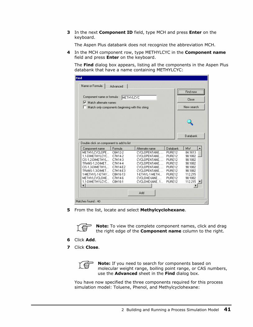
4 In the MCH component row, type METHYLCYC in the Component name field and press Enter on the keyboard.
The Find dialog box appears, listing all the components in the Aspen Plus databank that have a name containing METHYLCYC:
5 From the list, locate and select Methylcyclohexane.
Note: To view the complete component names, click and drag the right edge of the Component name column to the right.
6 Click Add.
7 Click Close.
Note: If you need to search for components based on molecular weight range, boiling point range, or CAS numbers, use the Advanced sheet in the Find dialog box.
You have now specified the three components required for this process simulation model: Toluene, Phenol, and Methylcyclohexane:

2 Building and Running a Process Simulation Model 42
8 Click .
The Properties | Specifications | Global sheet appears.
Selecting Thermodynamic Methods Use the Properties | Specifications | Global sheet to select the property method used to calculate properties such as K-values, enthalpy, and density. The Base method list contains all the property methods built into Aspen Plus. The size of the list may be reduced by specifying a particular Process type.
Note: Clicking the Modify property models checkbox allows you to create a custom property method that starts out identical to the chosen base method but may be modified according to your needs. For more information see the Aspen Plus User Guide, Chapter 7: Physical Property Methods.
For this simulation, use the UNIFAC property method to calculate thermodynamic properties.

2 Building and Running a Process Simulation Model 43
To Find the Appropriate Type of Base Method for this Simulation 1 In the Base method list, click to display the available property
methods in Aspen Plus:
Get a brief description of a base method by selecting it and reading the prompt. For detailed information about a base method, highlight the name and use the What�s this? help utility or refer to the Physical Property Methods and Models reference manual.
2 From the Base method list, use the vertical scrollbar and select UNIFAC.
2 Building and Running a Process Simulation Model 44
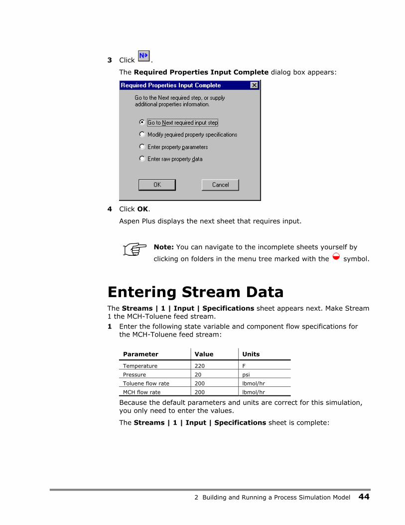
3 Click .
The Required Properties Input Complete dialog box appears:
4 Click OK.
Aspen Plus displays the next sheet that requires input.
Note: You can navigate to the incomplete sheets yourself by
clicking on folders in the menu tree marked with the symbol.
Entering Stream Data The Streams | 1 | Input | Specifications sheet appears next. Make Stream 1 the MCH-Toluene feed stream.
1 Enter the following state variable and component flow specifications for the MCH-Toluene feed stream:
Parameter Value Units
Temperature 220 F
Pressure 20 psi
Toluene flow rate 200 lbmol/hr
MCH flow rate 200 lbmol/hr
Because the default parameters and units are correct for this simulation, you only need to enter the values.
The Streams | 1 | Input | Specifications sheet is complete:

2 Building and Running a Process Simulation Model 45
2 Click .
The Streams | 2 | Input | Specifications sheet appears. Make Stream 2 the phenol feed stream.
3 Enter the following specifications for Stream 2:
Parameter Value Units
Temperature 220 F
Pressure 20 psi
Phenol flow rate 1200 lbmol/hr
4 Click .
The Blocks | B1 | Setup | Configuration sheet appears:

2 Building and Running a Process Simulation Model 46
Entering Unit Operation Block Data On the Blocks | B1 | Setup | Configuration sheet, the number of stages, the condenser type, and two operating specifications are required data. The reboiler type, valid phases, and convergence method have default choices displayed in shaded type.
1 Click each box and read the descriptive prompts at the bottom of the sheet.
If you click while the sheet is incomplete, the Completion Status message box appears indicating the missing specifications:
Click to close the Completion Status dialog box.
2 Enter the following specifications for the column:
Parameter Value Units
Number of stages 22 �
Condenser Total �
Distillate rate 200 lbmol/hr
Reflux ratio 8 �
Accept the defaults in the Reboiler, Valid phases, and Convergence fields.
The blue checkmark on the Configuration tab indicates the sheet is complete:

2 Building and Running a Process Simulation Model 47
3 Click or click the Streams tab.
The Blocks | B1 | Setup | Streams sheet appears.
In the RadFrac model, there are N stages. Stage 1 is the top stage (the condenser); stage N is the bottom stage (the reboiler). As shown in Figure 3.1, the MCH-Toluene feed (stream 1) enters above stage 14, and the phenol solvent stream (stream 2) enters above stage 7.
4 Enter 14 in the Stage field for Stream 1.
5 Enter 7 in the Stage field for Stream 2.
6 Accept the defaults for the entry point conventions for the feed streams and for the locations and phases of the product streams.
The Blocks | B1 | Setup | Streams sheet is complete:

2 Building and Running a Process Simulation Model 48
7 Click .
The Blocks | B1 | Setup | Pressure sheet appears.
You can enter a stage-by-stage profile, or specify a top-stage pressure and a pressure drop for the rest of the column. For this example, use a condenser pressure of 16 psi, and a reboiler pressure of 20.2 psi. Aspen Plus interpolates the pressure of the intermediate stages.
8 In the View list, click and select Pressure profile.
9 In the first Stage field, type 1 and then press the Tab key.
10 In the first Pressure field, type 16 and press Tab.
11 In the next Stage field, type 22 and press Tab.
12 In the next Pressure field, type 20.2.
13 Accept the default Pressure units (psi).
The completed Block B1 Setup Pressure sheet looks like this:
14 Click .
The Required Input Complete dialog box appears.
Note: You can enter additional specifications on optional input sheets, or go back to any of the required sheets and make changes. To see what optional input sheets are available, click Cancel on the dialog box and scroll through the Data Browser to view all the folders. The Reactions, Convergence, Flowsheeting Options, and Model Analysis Tools folders are optional.

2 Building and Running a Process Simulation Model 49
Running the Simulation 1 From the Required Input Complete dialog box, click OK.
The Control Panel appears and the simulation run begins:
Use the Control Panel to monitor and interact with the Aspen Plus simulation calculations. For more information on how to use the Control Panel, see the Aspen Plus User Guide, Chapter 11: Running Your Simulation, or see the topic Control Panel: about in the online help index.
As Aspen Plus executes the simulation, status messages appear in the Control Panel. When the simulation is complete, the message All blocks have been executed appears in the status bar.
Note: There are 3 tabs at the bottom of the active form that can be used to navigate between the overlapping windows. For example, to view the Process Flowsheet Window, click the
tab. If you don�t see the tabs, from the Window menu select Workbook.

2 Building and Running a Process Simulation Model 50
Examining Simulation Results When the simulation completes, the Results Available message appears in the status bar at the bottom of the main window. Now you can examine the results of your simulation.
1 Navigate to the process flowsheet in one of these ways:
− Click the Process Flowsheet tab, or − Select Window | Process Flowsheet Window from the Aspen Plus
menu bar.
To Display the Results for Block B1 2 In the process flowsheet, select either the block name B1 or the block
itself, then right-click to display the shortcut menu.
Note: Your flowsheet may now have some pressure and temperature data displayed. You can turn this feature on and off by selecting View | Global Data. You may also wish to alter the appearance of your flowsheet by selecting, for example, View | Zoom | Zoom Full.
3 From the shortcut menu, select Results.
The Block B1 Results Summary sheet appears:
For this run, block results are reported on three forms: Results Summary, Profiles, and Stream Results. In the Data Browser menu tree, a checkmark in a square appears next to each form to indicate that they contain results.

2 Building and Running a Process Simulation Model 51
4 From the Data Browser menu tree, select Blocks | B1 | Profiles by clicking once on either Profiles or its checkmark.
The Block B1 Profiles TPFQ sheet appears, reporting temperature, pressure, heat duty, and flow profiles for the block:
5 Use the scrollbar(s) to view the displayed profiles.
6 Click next to the View list and select Stage flows.
7 Use the Basis list to specify the type of units available for the displayed results.
8 Use the units box in each column to select the desired units for the display. Aspen Plus will perform the conversions automatically.
9 Use the Data Browser menu tree, the button, and/or the tabs on each form to view the rest of the results for Block B1.
10 Check the purity of the methylcyclohexane overhead product by examining the composition at the top of the column (stage 1).

2 Building and Running a Process Simulation Model 52
This simulation predicts a little better than 97% purity for the MCH product with the given stream and block specifications.

2 Building and Running a Process Simulation Model 53
Examining Stream Results Display calculated stream results by selecting a stream directly from the process flowsheet.
To Display the Results for Stream 3 1 Navigate to the process flowsheet.
2 Select Stream 3 and right-click to display the shortcut menu.
3 Select Results.
The Stream Results Material sheet appears, providing the results for Stream 3:
In addition to the thermodynamic state and flow results for the stream, mole fractions are also given (use the vertical scroll bar to view them) because you requested them by clicking the appropriate checkbox in the Setup | Report Options | Stream sheet.

2 Building and Running a Process Simulation Model 54
To Display the Results for All Streams on the Same Sheet 1 In the Stream Results Material sheet, click the list box at the top of the
first column of the data table (ignoring the field labels at the left) and select 1.
2 Click the list box in the second column and select 2.
3 Click the list box in the third column and select 3.
4 Click the list box in the fourth column and select 4.
The results for all four streams are displayed. A quicker way to do this is to select All streams in the Display list box.
Note: You can close or minimize some of the overlapping windows if you wish. Click the tab for a window and then use the lower row of control buttons in the upper right corner of the
screen: .
Changing Input Specifications In this section, review the effect of increasing the solvent flow rate on the purity and of the recovered methylcyclohexane.
To Increase the Phenol Solvent Stream Flow Rate 1 Navigate to the Process Flowsheet window.
2 Select Stream 2, and right-click to display the shortcut menu.
3 Select Input.
The Stream 2 Input Specifications sheet appears.
4 In the Composition area, change the flow rate for PHENOL from 1200 lbmol/hr to 1800 lbmol/hr by changing the entry in the Value field to 1800 and pressing Enter on the keyboard.
Since you have changed the input specifications, Input Changed messages appear in the prompt areas of the main window and in the Data Browser window. Also, the symbols and appear in several places in the Data
Browser menu tree. Finally, the run button and the Run | Run menu command are now enabled.

2 Building and Running a Process Simulation Model 55
Rerunning the Simulation with Changed Input 1 Click to continue.
The Required Input Complete dialog box appears indicating that your input is complete and asking if you want to run the simulation with the new specifications.
2 Click OK to run the simulation.
The Control Panel appears and the column calculations are completed using the new phenol flow rate.
3 Display the new block and stream results by either selecting blocks and streams from the process flowsheet as before or navigating using the Data Browser.
Note: You can display the complete Data Browser menu tree by
clicking the button, or by selecting Data | Data Browser from the Aspen Plus menu bar, or by pressing F8.
MCH purity with the increased phenol flow rate is now over 98%. To choose an optimal flow rate, it would be helpful to generate a plot of MCH purity versus phenol flow rate. This is the subject of Chapter 3: Performing a Sensitivity Analysis.
Creating Reports
To Generate a Report File Aspen Plus allows you to generate a report file containing the simulation specifications and calculated results.
1 From the Aspen Plus menu bar, select File and then select Export.
The Export dialog box appears.
2 In the Save as type list, click and select Report File (*.rep).
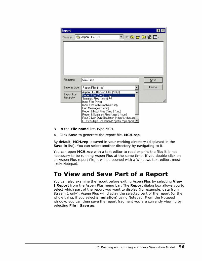
2 Building and Running a Process Simulation Model 56
3 In the File name list, type MCH.
4 Click Save to generate the report file, MCH.rep.
By default, MCH.rep is saved in your working directory (displayed in the Save in list). You can select another directory by navigating to it.
You can open MCH.rep with a text editor to read or print the file; it is not necessary to be running Aspen Plus at the same time. If you double-click on an Aspen Plus report file, it will be opened with a Windows text editor, most likely Notepad.
To View and Save Part of a Report You can also examine the report before exiting Aspen Plus by selecting View | Report from the Aspen Plus menu bar. The Report dialog box allows you to select which part of the report you want to display (for example, data from Stream 1 only). Aspen Plus will display the selected part of the report (or the whole thing, if you select simulation) using Notepad. From the Notepad window, you can then save the report fragment you are currently viewing by selecting File | Save as.

2 Building and Running a Process Simulation Model 57
Saving Your File and Exiting Aspen Plus 1 From the Aspen Plus menu bar, select File | Save as.
2 In the File name field, type MCH. Make sure the Save as type field reads Aspen Plus Documents (*.apw) and click Save.
Aspen Plus saves the simulation in your working folder.
Note: This folder is located in C:\Program Files\AspenTech\Working Folders\Aspen Plus 2004.1 if C:\Program Files\AspenTech is the Root Directory selected when Aspen Plus was installed.
3 Select File | Exit to exit Aspen Plus.
Chapters 3 and 5 use MCH.apw as their starting point.

3 Performing a Sensitivity Analysis 58
3 Performing a Sensitivity Analysis
One of the benefits of a simulation is that you can study the sensitivity of process performance to changes in operating variables. With Aspen Plus, you can allow inputs to vary, and can tabulate the effect on a set of results of your choice. This procedure is called a sensitivity analysis.
In this chapter, you will perform a sensitivity analysis using either the methylcyclohexane (MCH) recovery simulation you created in Chapter 2 or the MCH simulation that was placed in the Examples folder when you installed Aspen Plus.
Allow about 20 minutes for this simulation.
Starting Aspen Plus 1 From your desktop, select Start and then select Programs.
2 Select AspenTech | Aspen Engineering Suite | Aspen Plus 2004.1| Aspen Plus User Interface.
The Aspen Plus Startup dialog box appears.

3 Performing a Sensitivity Analysis 59
Opening an Existing Simulation You can open a saved simulation file from the list presented at startup, or by navigating to a folder containing the saved file. For this session, either open your saved MCH.apw from Chapter 2, or use MCH.bkp in the Examples folder.
If Your Saved File MCH.apw is Displayed To open an existing simulation:
1 In the Aspen Plus Startup dialog box, make sure Open an Existing Simulation is selected.
2 In the list, select MCH.apw and click OK.
-or-
If Your Saved File MCH.apw is not Displayed 1 In the Aspen Plus Startup dialog box, make sure Open an Existing
Simulation is selected.
2 In the list box, double-click More Files, or click OK without selecting anything in the list box.
The Open dialog box appears.
3 Navigate to the directory containing your saved MCH.apw or navigate to the Examples folder containing MCH.bkp.
Note: The Examples folder is located in: C:\Program Files\AspenTech\Aspen Plus\Favorites\Examples if C:\Program Files\AspenTech is the Root Directory selected when Aspen Plus was installed.
4 Select either MCH.apw or MCH.bkp and click Open.
Note: If the Connect to Engine dialog box appears, see Chapter 8.
The Process Flowsheet window for the MCH column simulation appears.

3 Performing a Sensitivity Analysis 60
Saving a Simulation under a New Name Before creating a new simulation from MCH.apw or MCH.bkp, create a file with a new name, MCHSENS.apw. Now you can modify this new file. The original is safe.
1 From the Aspen Plus menu, select File and then Save As.
2 In the Save As dialog box, choose the directory where you want to save the simulation.
3 In the File name field, enter MCHSENS.
4 In the Save as type field, make sure Aspen Plus Documents (*.apw) is selected.
5 Click Save.
Defining the Sensitivity Analysis In Chapter 2, you simulated MCH recovery using two values for the phenol solvent flow rate. In the following sensitivity analysis, tabulate methylcyclohexane (MCH) distillate product purity (mole fraction), as well as condenser duty and reboiler duty, for several different flow rates of phenol.
Entering Sensitivity Specifications
To Create a New Sensitivity Block 1 Select Data | Model Analysis Tools | Sensitivity.
The Model Analysis Tools | Sensitivity object manager appears. You can use this sheet to:
− Create new sensitivity blocks. − Edit existing sensitivity blocks. − View status of sensitivity blocks.
2 Click New.
The Create new ID dialog box appears.
3 Click OK to accept the default ID (S-1).
The Model Analysis Tools | Sensitivity | S-1 | Input | Define sheet appears:

3 Performing a Sensitivity Analysis 61
This sensitivity analysis will generate a data table. The first column will contain a user-specified range of input values for the phenol flow rate. Three other columns will contain calculated results for MCH distillate product purity, the condenser duty, and the reboiler duty.
In the Define sheet, define names for each of the calculated variables (product purity, condenser duty, reboiler duty). In the Vary sheet, specify the range and increments for the manipulated variable (phenol flow rate). In the Tabulate sheet, set up the format you want for the data table.
Start with the definition of the MCH distillate product purity variable.
To Define XMCH as Distillate Product Purity 1 On the Define sheet, click New.
The Create new variable dialog box appears.
2 Type XMCH and click OK.
The Variable Definition dialog box appears. Define XMCH to be the mole fraction of MCH in Stream 3 as follows.
3 In the Category area, select Streams.
4 In the Reference area, click the Type field and select Mole-Frac.
As you complete the specifications in this dialog box, more fields necessary to complete the variable definition will appear.
5 In the Stream field, select 3.
In this simulation, you do not need to modify the default value of MIXED in the Substream field.
6 In the Component field, select MCH.

3 Performing a Sensitivity Analysis 62
You have defined XMCH to be the mole fraction of MCH in Stream 3. The blue checkmarks indicate that the variable specification is complete.
7 Click Close.
The Model Analysis Tools | Sensitivity S-1 | Input | Define sheet reappears with the first defined variable, XMCH, listed.
Next, define the condenser duty and reboiler duty variables.
To Define QCOND as the Condenser Duty and QREB as Reboiler Duty 1 Click New again.
The Create new variable dialog box appears.
2 Type QCOND and click OK.
The Variable Definition dialog box appears. Define QCOND to be the condenser duty for the RadFrac Block B1.
3 In the Category area, select Blocks.
4 In the Type field, select Block-Var.
5 In the Block field, select B1.
6 In the Variable field, click the drop down button to show the list of variables.
Judging by the size of the scroll bar, the list of variables is quite long. For complex unit operation models like RadFrac, it can be difficult to find the intended variable. Aspen Plus offers a search capability to help you find the correct variable.

3 Performing a Sensitivity Analysis 63
7 Click the icon next to the Variable list
The Search Variables dialog box appears. You can search on any string that you think might help to reduce the number of variables.
8 In the Search criteria area, enter Condenser Duty.
Aspen Plus searches for variables that contain the words Condenser and Duty in the variable name or variable description. The search is not case sensitive. Aspen Plus identifies the following variables:
9. Double click COND-DUTY to select it as the simulation variable linked to the variable you have named QCOND.
Aspen Plus automatically fills in the Variable field and the Sentence field, based on your choice of variable. Aspen Plus also shows the units of measure for the accessed variable (Btu/hr).
Note: The units of measure for accessed variables depend on the units of measurement of the object that contains the defined variables. Since this Sensitivity blocks uses ENG units, heat duties have the units of Btu/hr. If you were to toggle the units to SI in the Menu bar, the heat duties would be accessed in Watts.
Do not close the dialog box. Instead, define the next variable, QREB.
10 In the Variable name field, select <New>.
Note: You can also right-click on the Variable name field and from the shortcut menu, select Create.
The New Item dialog box appears.
11 Type QREB and click OK.
Define QREB to be the reboiler duty for Block B1.

3 Performing a Sensitivity Analysis 64
12 In the Category area, select Blocks.
13 In the Type field, select Block-Var.
14 In the Block field, select B1.
15 Click next to the Variable list, and search for Reboiler Duty.
16 Double click REB-DUTY to select it as the simulation variable linked to the variable you have named QREB.
Aspen Plus fills in the Variable, Sentence and units of measure for QREB.
17 Click Close.
You have now defined QCOND and QREB to be the condenser duty and reboiler duty for block B1.
The Model Analysis Tools | Sensitivity | S-1 | Input | Define sheet reappears with the three defined calculated variables, XMCH, QCOND, and QREB listed.
Next, specify the range, increment size, and label for the phenol flow rate manipulated variable.
To Specify the Manipulated Variable 1 Click or click the Vary tab.
The Model Analysis Tools | Sensitivity | S-1 | Input | Vary sheet appears.
Define the phenol flow rate (Stream 2) to vary from 1200 lbmol/hr to 2000 lbmol/hr in increments of 100 lbmol/hr.
2 In the Variable number field, select 1.
3 In the Type field, select Stream-Var.
4 In the Stream field, select 2.
Like the Define sheet, the Vary sheet has a search button to help you
select the correct variable. While you could click and search for Mole Flow, the list of Stream Variables is not very long, so you may find it easier to pick from a list. Both methods of identifying and selecting variables are acceptable.
5 In the Variable field, select MOLE-FLOW.
6 In the Values for varied variable area, select Overall range and enter the following values:
Field Value
Lower 1200
Upper 2000
Incr 100

3 Performing a Sensitivity Analysis 65
7 In the Report labels area, you have the option of entering up to four lines to be used as a column header in the Sensitivity table. Enter the following report labels:
Line Value
Line 1 PHENOL
Line 2 FLOWRATE
You have completely specified the phenol flow rate as a manipulated variable for this sensitivity analysis:
Next, specify the format for the table that Aspen Plus will produce when you run the analysis.

3 Performing a Sensitivity Analysis 66
To Format the Tabular Results 1 Click or click the Tabulate tab.
The Model Analysis Tools | Sensitivity | S-1 | Input | Tabulate sheet appears. You must identify the variables that you want to appear in the Sensitivity table.
2 Press the Fill Variables button to have Aspen Plus tabulate all of the Defined variables automatically.
The completed sheet looks like this:
Note: You could have filled out the same information manually. You can also tabulate mathematical expressions written using Fortran notation.
3 Click Table Format.
The Table Format dialog box appears. Enter column labels for columns 1, 2, and 3, whose data contents were defined above.
Labels are split into 4 lines for the report file. Each line can contain up to 8 characters.
4 In column 1 type MCH PURITY IN DIST using 3 lines.
5 In column 2 type CONDENS DUTY using 2 lines.

3 Performing a Sensitivity Analysis 67
6 In column 3 type REBOILER DUTY using 2 lines.
The completed dialog box looks like this:
7 Click Close.
The Model Analysis Tools | Sensitivity | S-1 | Input form is complete and you are ready to run the sensitivity analysis.
Running the Sensitivity Analysis Run the simulation in any of the following ways:
• From the Aspen Plus menu bar, select Run, and then select Run.
• From the Aspen Plus toolbar, click .
• Click to open the Control Panel and then click from the Control Panel.
• Press F5.
Now you can display and plot the results.

3 Performing a Sensitivity Analysis 68
Displaying Sensitivity Analysis Results The Sensitivity Analysis Results consist of a table of the values you requested on the Input | Tabulate sheet, shown as a function of the manipulated variable defined on the Input | Vary sheet.
1 From the Data Browser menu tree, click Model Analysis Tools | Sensitivity | S-1 | Results.
The Model Analysis Tools Sensitivity S-1 Results Summary sheet appears:
Note: The above results were obtained using the Aspen Plus document file, mch.apw. If you used the Aspen Plus backup file, mch.bkp, from the Examples folder, your results may be slightly different (in the 3rd significant digit or beyond). These differences occur because the starting points for the iterative calculations are different. When you use an .apw file, Aspen Plus starts calculating from the previous results. When you use a .bkp file, Aspen Plus reinitializes before starting calculations.

3 Performing a Sensitivity Analysis 69
Plotting Sensitivity Results Make a plot of MCH purity vs. phenol flow rate.
To Generate a Plot of MCH Distillate Purity Versus Phenol Flow Rate 1 Select the VARY 1 PHENOL FLOWRATE column by clicking its label.
2 From the Plot menu, select X-Axis Variable.
3 Select the MCH PURITY IN DIST column by clicking its label.
4 From the Plot menu, select Y-Axis Variable.
5 From the Plot menu, select Display Plot.
A new window with its own tab appears containing the plot you specified.
6 Click in the lower set of control buttons in the upper right corner to reduce the size of the plot and give it a separate window.
The reduced-sized plot looks like this:
7 If you wish, customize the plot by clicking the right mouse button in the Plot window to access the plot menu.

3 Performing a Sensitivity Analysis 70
Saving Your File and Exiting Aspen Plus 1 From the Aspen Plus menu bar, select File | Save as.
2 In the File name field, type MCHSENS. Make sure the Save as type field reads Aspen Plus Documents (*.apw) and click Save.
Aspen Plus saves the simulation in your working folder.
Note: This folder is located in C:\Program Files\AspenTech\Working Folders\Aspen Plus 13.1 if C:\Program Files\AspenTech is the Root Directory selected when Aspen Plus was installed.
3 Select File | Exit to exit Aspen Plus.
Chapter 4 uses MCHSENS.apw as its starting point.
4 Meeting Process Design Specifications 71
4 Meeting Process Design Specifications
In Chapter 3, you used Aspen Plus to tabulate the sensitivity of MCH distillate purity and column duties to changes in phenol solvent flow rate. You can also use Aspen Plus to meet a specific process design target (or design specification) by manipulating any simulation input variable.
In this chapter, you will use Aspen Plus to meet a process design specification using either the methylcyclohexane (MCH) recovery simulation you created in Chapter 2 or the MCH simulation that was placed in the Examples folder when you installed Aspen Plus.
Allow about 20 minutes for this simulation.
Starting Aspen Plus 1 From your desktop, select Start and then select Programs.
2 Select AspenTech | Aspen Engineering Suite | Aspen Plus 2004.1 | Aspen Plus User Interface.
The Aspen Plus Startup dialog box appears.
Opening an Existing Simulation You can open a saved simulation file from the list presented at startup, or by navigating to a folder containing the saved file. For this session, either open your saved MCHSENS.apw from Chapter 3, or use MCHSENS.bkp in the Examples folder.
If Your Saved MCHSENS.apw is Displayed To open an existing simulation:
1 In the Aspen Plus Startup dialog box, make sure Open an Existing Simulation is selected
2 In the list, select MCHSENS.apw and click OK.

4 Meeting Process Design Specifications 72
-or-
If Your Saved File MCHSENS.apw is Not Displayed 1 In the Aspen Plus Startup dialog box, make sure Open an Existing
Simulation is selected
2 In the list box, double-click More Files, or click OK without selecting anything in the list box.
The Open dialog box appears.
3 Navigate to the directory containing your saved MCHSENS.apw or navigate to the Examples folder containing MCHSENS.bkp.
Note: The Examples folder is located in: C:\Program Files\AspenTech\Aspen Plus 2004.1\Favorites\Examples if C:\Program Files\AspenTech is the Root Directory selected when Aspen Plus was installed.
4 Select either MCHSENS.apw or MCHSENS.bkp and click Open.
Note: If the Connect to Engine dialog box appears, see Chapter 8.
The Process Flowsheet window for the MCH column simulation appears.
Saving a Simulation Under a New Name Before creating a new simulation from MCHSENS.apw or MCHSENS.bkp, create a file with a new name, MCHSPEC.apw. Now you can modify this new file. The original is safe.
1 From the Aspen Plus menu, select File | Save As.
2 In the Save As dialog box, choose the directory where you want to save the simulation.
3 In the File name field, enter MCHSPEC.
4 In the Save as type field, make sure Aspen Plus Documents (*.apw) is selected.
5 Click Save.

4 Meeting Process Design Specifications 73
Defining the Design Specification In Chapter 2, you simulated MCH recovery using two values for the phenol solvent flow rate. In the sensitivity analysis in Chapter 3, you tabulated MCH distillate product purity, and condenser and reboiler duties, as a function of phenol solvent flow rate.
Now use Aspen Plus to determine the exact phenol solvent feed rate required to maintain an MCH distillate purity of 98.0%.
To Enter Design Specifications 1 Select Data | Flowsheeting Options | Design Spec.
The Design Spec object manager appears.
2 Click New.
The Create New ID dialog box appears
3 Click OK to accept the default ID (DS-1).
The Flowsheeting Options | Design Spec | DS-1 | Define sheet appears:
In the Define sheet, define XMCH to be the MCH purity. In the Spec sheet, enter the specification as a mathematical expression containing numbers and defined variables, and also enter a target value for this expression and a tolerance. In the Vary sheet, specify an input variable to be manipulated and a range in which Aspen Plus will search in order to obtain the target value given on the Spec sheet.
Start with the definition of XMCH as the mole fraction of MCH in Stream 3.
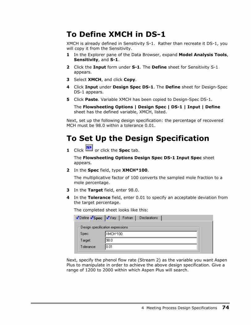
4 Meeting Process Design Specifications 74
To Define XMCH in DS-1 XMCH is already defined in Sensitivity S-1. Rather than recreate it DS-1, you will copy it from the Sensitivity.
1 In the Explorer pane of the Data Browser, expand Model Analysis Tools, Sensitivity, and S-1.
2 Click the Input form under S-1. The Define sheet for Sensitivity S-1 appears.
3 Select XMCH, and click Copy.
4 Click Input under Design Spec DS-1. The Define sheet for Design-Spec DS-1 appears.
5 Click Paste. Variable XMCH has been copied to Design-Spec DS-1.
The Flowsheeting Options | Design Spec | DS-1 | Input | Define sheet has the defined variable, XMCH, listed.
Next, set up the following design specification: the percentage of recovered MCH must be 98.0 within a tolerance 0.01.
To Set Up the Design Specification 1 Click or click the Spec tab.
The Flowsheeting Options Design Spec DS-1 Input Spec sheet appears.
2 In the Spec field, type XMCH*100.
The multiplicative factor of 100 converts the sampled mole fraction to a mole percentage.
3 In the Target field, enter 98.0.
4 In the Tolerance field, enter 0.01 to specify an acceptable deviation from the target percentage.
The completed sheet looks like this:
Next, specify the phenol flow rate (Stream 2) as the variable you want Aspen Plus to manipulate in order to achieve the above design specification. Give a range of 1200 to 2000 within which Aspen Plus will search.

4 Meeting Process Design Specifications 75
To Specify the Manipulated Variable 1 Click or click the Vary tab.
The Flowsheeting Options | Design Spec | DS-1 | Input | Vary sheet appears.
2 In the Manipulated variable area, click the Type field and select Stream-Var.
3 In the Stream name field, select 2.
4 In the Substream field, accept the default, MIXED.
5 In the Variable field, select MOLE-FLOW.
6 In the Manipulated variable limits area, click the Lower field and type 1200.
7 In the Upper field type 2000.
8 In the Report Labels area, click the Line 1 field and type PHENOL.
9 In the Line 2 field, type FLOWRATE.
The completed sheet looks like this:
The Flowsheeting Options Design Spec DS-1 form is complete. However, Sensitivity S-1 still exists. Before running the design specification analysis, you must hide Sensitivity S-1.
1. Select Data | Model Analysis Tools | Sensitivity. The Sensitivity Object Manager Appears.
2. Select row S-1, and click Hide. Sensitivity S-1 disappears from the object manager. Hidden objects no longer have an active role in the current simulation.

4 Meeting Process Design Specifications 76
Note: Many of the object managers in Aspen Plus have the capability to hide individual objects. If an object manager has hidden objects, the Reveal button will be active. Click the Reveal button to reveal one or more hidden objects.
You are ready to run the design specification analysis and examine the results.
Running the Design Specification Analysis Run the analysis in any of the following ways:
• From the Aspen Plus menu bar, select Run | Run.
• From the Aspen Plus toolbar, click .
• Click to open the Control Panel and then click from the Control Panel.
• Press F5.
Then examine the results.

4 Meeting Process Design Specifications 77
Examining Design Specification Results Determine how well your design specification has been satisfied by examining the Results Summary | Convergence | Design Spec Summary sheet.
1 From the Data Browser menu tree, click Results Summary | Convergence.
The Results Summary Convergence DesignSpec Summary sheet appears:
The results show that that the calculation converged successfully and that the necessary value of the phenol flow rate is approximately 1517.1. The units, lbmol/hr, are not shown.
Note: The above results were obtained by using the Aspen Plus document file, MCH.apw. If you used the Aspen Plus backup file, MCH.bkp, from the Examples folder, your results may be slightly different (in the 3rd significant digit and beyond). These differences occur because the starting point for the calculations are different. When you use a document (.apw) file, Aspen Plus starts calculating from the previous results. When you use a backup (.bkp) file, Aspen Plus reinitializes before starting calculations.
Exiting Aspen Plus 1 From the Aspen Plus menu bar, click File | Exit.
The Aspen Plus dialog box appears.
2 Click Yes to save the simulation.

5 Creating a Process Flow Diagram 78
5 Creating a Process Flow Diagram
Aspen Plus has two modes for displaying graphics:
• Simulation mode
• PFD (Process Flow Diagram) mode
In both modes, you can modify your process flowsheet to prepare customized drawings for reports by:
• Adding text and graphics
• Displaying global data for streams and blocks
• Displaying stream results tables
• Adding OLE objects
In PFD mode, you can modify the flowsheet to match your plant. For example, a single piece of equipment in the plant that is modeled by two unit operation blocks can be replaced by a single block in PFD mode. These changes are for display purposes and do not affect the flowsheet you developed to model your process.
In this chapter, you will use PFD mode to generate a plant diagram from the process flowsheet you used in the MCH simulation. You can use the file created in Chapter 2 or the simulation that was saved in the Examples folder when you installed Aspen Plus.
Allow about 20 minutes for this example.
Starting Aspen Plus 1 From your desktop, select Start and then select Programs.
2 Select AspenTech | Aspen Engineering Suite | Aspen Plus 2004.1 | Aspen Plus User Interface.
The Aspen Plus Startup dialog box appears.

5 Creating a Process Flow Diagram 79
Opening an Existing Simulation You can open a saved simulation file from the list presented at startup, or by navigating to a folder containing the saved file. For this session, either open your saved MCH.apw from Chapter 2, or use MCH.bkp in the Examples folder.
If Your Saved File MCH.apw is Displayed To open an existing simulation:
1 In the Aspen Plus Startup dialog box, make sure Open an Existing Simulation is selected.
2 In the list, select MCH.apw and click OK.
-or-
If Your Saved File MCH.apw is not Displayed 1 In the Aspen Plus Startup dialog box, make sure Open an Existing
Simulation is selected.
2 In the list box, double-click More Files, or click OK without selecting anything in the list box.
The Open dialog box appears.
3 Navigate to the directory containing your saved MCH.apw or navigate to the Examples folder containing MCH.bkp.
Note: The Examples folder is located in: C:\Program Files\AspenTech\Aspen Plus\Favorites\Examples if C:\Program Files\AspenTech is the Root Directory selected when Aspen Plus was installed.
4 Select either MCH.apw or MCH.bkp and click Open.
Note: If the Connect to Engine dialog box appears, see Chapter 8.
The Process Flowsheet window for the MCH simulation appears.

5 Creating a Process Flow Diagram 80
Switching to PFD Mode Simulation mode is the Aspen Plus default mode that you use to model a process or perform calculations. PFD mode is used to create a graphical representation of your process for a report or for display purposes. Use PFD mode to do the following:
• Add equipment icons and streams that were not explicitly included in the simulation.
• Display stream data.
• Display a results table.
• Add a title.
To toggle between Simulation Mode and PFD Mode, use either of the following methods:
• Select View | PFD Mode.
• Press F12.
The check mark next to PFD Mode in the View menu and the status bar at the bottom of the main window indicate that PFD mode is on. Also, the process flowsheet workspace has a thick colored border when you are using PFD mode.
When you select PFD mode, Aspen Plus creates a new graphic identical to the original flowsheet. This new graphic is independent of the original. Making changes to streams and blocks in either one and toggling modes will show that these changes do not cross over.
Note: If you change the original process flowsheet model and you wish to start over again with a new PFD style drawing that contains these changes, select View | Reset PFD while in PFD mode. Your old PFD will be deleted and it will be replaced by a new drawing identical to the process flowsheet from your revised simulation model.
Adding a Pump to the Diagram In the MCH simulation, you did not model the feed pump to the column; instead, you simply specified the pressure in the feed stream. However, you may wish to include a feed pump in a drawing used for a report or display.
Place a pump in your diagram and split Stream 1 into two streams � one entering the pump and one leaving the pump and entering Block B1. Follow the directions below.

5 Creating a Process Flow Diagram 81
To Add the Feed Pump to the PFD Diagram 1 Enter PFD Mode by selecting View | PFD Mode if you have not already
done so. Look for the colored border on the process flowsheet and the words PFD Mode in the bottom status bar to ensure you are in PFD Mode.
2 From the Model Library, click the Pressure Changers tab.
3 Click next to the Pump unit operation model.
4 Hover over the icons to see their labels and select ICON1.
5 Drag (click and hold) the selected icon to the Process Flowsheet window to create Pump block B2.
6 Place the pump icon in the middle of Stream 1.
7 Click to stop adding the unit operation model.
To Insert the Pump Into the Feed Stream 8 Select Stream 1 and right-click.
9 From the shortcut menu, select Reconnect Destination.
Stream 1 is now disconnected from Block B1 and you are ready to reconnect it to the pump.
10 Move the cursor arrowhead to an inlet port on the pump and left-click.
Stream 1 now enters the pump and you are ready to create a new stream from the pump to Block B1.
11 Click once on on the left side of the Model Library.
12 Move the cursor (now a crosshair ) to an outlet port on the pump and click once.
13 Move the cursor (now an arrowhead ) to a feed port on Block B1 and click once to create a fifth stream.
Note: To cancel connecting the stream at any time, press ESC.

5 Creating a Process Flow Diagram 82
Your diagram should look something like this:
The Block names B1 and B2 have been moved for clarity. If you wish, you may also rename Stream 5 to Stream 1 or Stream 1A since the pump doesn�t change the components of the stream.
Once you are satisfied with the layout, you can lock the existing layout to prevent accidental movement of blocks or streams.
From the Flowsheet pulldown menu, select Lock. Locking the flowsheet applies to both PFD mode and normal mode.
Note: If you make a mistake while working with the graphics, it is easy to Undo the mistake. From the Edit menu, select Undo. The Undo only applies to the graphical flowsheet (placing a block, moving a stream, etc.). Due to limitations in the GUI architecture, the Undo button cannot be used to Undo changes to the forms.

5 Creating a Process Flow Diagram 83
Displaying Stream Data
To Display Temperature and Pressure 1 From the View menu, ensure that Global Data has a checkmark next to
it.
2 Select Tools | Options | Results View.
3 Select the Temperature and Pressure checkboxes.
4 Click OK.
The temperature and pressure calculated by Aspen Plus during the MCH simulation run are shown on each stream. Aspen Plus also displays a legend box in the lower left corner of the screen. The legend box shows the symbols and units for the global data. Move and resize the legend in the same way that you move and resize blocks.
Note: If you do not see the legend box, select View | Zoom | Zoom Full or press Ctrl-End to see the whole drawing.
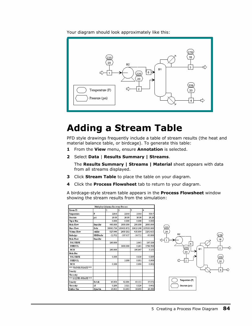
5 Creating a Process Flow Diagram 84
Your diagram should look approximately like this:
Adding a Stream Table PFD style drawings frequently include a table of stream results (the heat and material balance table, or birdcage). To generate this table:
1 From the View menu, ensure Annotation is selected.
2 Select Data | Results Summary | Streams.
The Results Summary | Streams | Material sheet appears with data from all streams displayed.
3 Click Stream Table to place the table on your diagram.
4 Click the Process Flowsheet tab to return to your diagram.
A birdcage-style stream table appears in the Process Flowsheet window showing the stream results from the simulation:
5 Creating a Process Flow Diagram 85
Note: The table is scaled for printing.
You can zoom in on various parts of the diagram by enclosing an area and selecting Zoom In from the shortcut menu. See the directions below.
To Zoom in on Part of the Diagram 1 Drag the cursor (clicking and holding) across the area you would like to
magnify.
2 When you have enclosed the area, release the cursor. It will be surrounded by a box.
3 With the cursor in the selected region, right-click to display the shortcut menu.
4 From the shortcut menu, select Zoom In.
Adding Text Add a title to the drawing using the Draw toolbar.
To Display the Draw Toolbar 1 Select View | Toolbar.
2 In the Toolbars dialog box, select the Draw checkbox.
3 Click OK.
The Draw toolbar appears.
To Add Text
4 From the Draw toolbar, click .
5 Move the cursor to an appropriate spot for the text and left-click.
A rectangular box with a blinking cursor appears.
6 Type Methylcyclohexane Recovery Column, then click outside the rectangular box.
7 Select the title and change the font size to 28 using the Draw toolbar.
8 Click the title and hold the mouse button down until the cursor changes shape, then drag the title anywhere you like.
9 Select View | Zoom Full.

5 Creating a Process Flow Diagram 86
The final diagram looks like something like this:
Printing a Process Flow Diagram Before you print, make sure that your printer is set up correctly. Refer to the online help topic Using Aspen Plus | Annotating Process Flowsheets, or to the Aspen Plus User Guide, Chapter 14, for more information on printing options.
To Preview Your Drawing Before Printing 1 Select File | Print Preview.
The block and stream IDs and the global data in your drawing are now scaled approximately as they will appear in print.
2 Click Zoom In or Zoom Out.
To Print the PFD-Style Drawing 3 Click Print.
The Print dialog box appears asking you where you want the output directed.
4 Select the appropriate printer and click OK.

5 Creating a Process Flow Diagram 87
Leaving PFD Mode You have seen how straightforward it is to create a PFD-style drawing from a process flowsheet. Remember that the modifications you have made for the PFD-style drawing have no effect on the process flowsheet and will not be included in it.
To Return to Simulation Mode 1 Select View | PFD Mode or press F12 to toggle PFD mode off and return
to simulation mode.
The original process flowsheet is displayed without the pump, but with the stream pressure and temperature data, the results table, and the title that you added in PFD mode.
2 Select View | Global Data to toggle it off if you don�t want to view the table and the pressure and temperature data in the original process flowsheet.
3 Select View | Annotation to toggle it off if you don�t want to view the title in the original process flowsheet.
Note: Remember, the streams and blocks in the PFD drawing and the process flowsheet are independent of one another unless you select View | Reset PFD while in PFD mode.
Exiting Aspen Plus 1 Select File | Exit.
The Aspen Plus dialog box appears.
2 Click Yes to save the simulation.

6 Estimating Physical Properties for a Non-Databank Component 88
6 Estimating Physical Properties for a Non-Databank Component
This chapter guides you through the procedure for estimating physical properties for a component that is not present in the Aspen Plus databank.
You will use a known molecular structure and known properties of Thiazole to provide Aspen Plus with a starting point for estimating missing properties.
Allow about 30 minutes for this simulation.
Thiazole Physical Property Data In this simulation, you are dealing with a process involving Thiazole and water, among other components.
Thiazole (C3H3NS) is not in the Aspen Plus databank. The following information is available from various sources:
Molecular structure for Thiazole:
HC=CH
N=CH S
Molecular weight: 85
Normal boiling point: 116.8 °C
Vapor pressure correlation:
ioLpln = 16.445 - 3281.0/(T+216.255)
For poLi in mmHg, T in °C for 69 °C < T < 118°C
By checking the manual Aspen Plus Physical Property Methods and Models, Chapter 3, you see that you do not have data for all the required pure component property parameters for Thiazole. You are missing data for the following property parameters (required for calculating enthalpies and densities):

6 Estimating Physical Properties for a Non-Databank Component 89
Parameter Description
TC Critical temperature
PC Critical pressure
CPIG Ideal gas heat capacity coefficients
DHFORM Heat of formation
DGFORM Gibbs free energy formation
DHVLWT Watson heat-of-vaporization coefficients
VC Critical volume
ZC Critical compressibility factor
Run a Property Estimation simulation in Aspen Plus to estimate the missing property parameters for Thiazole required to run your simulation.
Starting Aspen Plus 1 From your desktop, select Start and then select Programs.
2 Select AspenTech | Aspen Engineering Suite | Aspen Plus 2004.1 | Aspen Plus User Interface.
The Aspen Plus Startup dialog box appears.
3 From the Aspen Plus Startup dialog box, select Template and click OK.
The New dialog box appears.
Creating a Property Estimation Simulation Use the New dialog box to specify the application type and the run type for the new simulation.
1 From the New dialog box, select the General with English Units application type.
2 In the Run Type field, click and select Property Estimation.
3 Click OK.
Note: If the Connect to Engine dialog box appears, see Chapter 8.
The Data Browser appears. There is no process flowsheet for a Property Estimation run. First enter a title for the simulation. Then define a new component with the name thiazole and tell Aspen Plus to estimate all missing properties. Then enter the molecular structure of Thiazole and all known properties. Then run the estimation.

6 Estimating Physical Properties for a Non-Databank Component 90
Entering a Title 1 Expand the Setup folder in the Data Browser menu tree and click
Specifications.
The Setup | Specifications | Global sheet appears. The run type Property Estimation is already selected.
2 In the Title field, type Property Estimation for Thiazole.
Next, define a component called THIAZOLE.
Entering Components Information 1 Expand the Components folder in the Data Browser menu tree and click
Specifications.
The Components | Specifications | Selection sheet appears.
2 In the first line of the Component ID column, enter THIAZOLE.
Because THIAZOLE is not in the Aspen Plus databank, do not fill in the Component name or Formula columns.

6 Estimating Physical Properties for a Non-Databank Component 91
Next, tell Aspen Plus to estimate all missing properties.

6 Estimating Physical Properties for a Non-Databank Component 92
Specifying Properties to Estimate 1 Expand the Properties folder and the Estimation folder and click Input.
The Properties Estimation Input Setup sheet appears.
2 Accept the default Estimation option Estimate all missing parameters.
The other sheets on this form allow you to select specific estimation methods for each property if you do not wish to use the default methods. For this example, the defaults are adequate.
Next, enter the molecular structure of Thiazole. Click .

6 Estimating Physical Properties for a Non-Databank Component 93
Entering Molecular Structure The Non-Databank Components dialog box appears, indicating that your simulation has some non-databank components, for which you can enter additional information.
To Enter the Molecular Structure Information for Thiazole 1 Click Cancel.
2 Expand the Properties | Molecular Structure folder in the Data Browser menu tree and click THIAZOLE.
The Properties | Molecular Structure | THIAZOLE | General sheet appears:
Note: You can define the molecular structure either by using the General Method which is based on individual atoms and bonds, or by using the Functional Group Method in which you indicate the functional groups specific to a particular estimation method. This example explains how to use the General Method.
On the General sheet, specify the molecular structure of Thiazole by listing each non-hydrogen atom and each bond. Aspen Plus handles the hydrogen.

6 Estimating Physical Properties for a Non-Databank Component 94
3 Sketch the structure of Thiazole and number all the non-hydrogen atoms:
C = C1 2
N = C5 4
S3
Each atom will be listed twice, once as an atom that connects (Atom 1) and once as an atom that is connected to (Atom 2).
4 Enter the following information for Atom 1:
Number Type
1 C
2 C
3 S
4 C
5 N
This table associates each number with type of atom.
5 Enter the following information for Atom 2:
Number Type (generated automatically)
2 C
3 S
4 C
5 N
1 C
This table indicates which atom is connected to each of the atoms in the first table.

6 Estimating Physical Properties for a Non-Databank Component 95
6 In the Bond type column, select Double bond between atoms 1 and 2 and between 4 and 5, and select Single bond for the other bonds.
The Properties Molecular Structure THIAZOLE General sheet is now complete:
Next, enter the known property data for thiazole.
Entering Property Data The molecular structure information is sufficient for Aspen Plus to estimate properties. However, entering all available data will improve the accuracy of the Aspen Plus estimation.
To Enter Pure Component Boiling Point and Molecular Weight for Thiazole 1 Expand the Properties | Parameters folder in the Data Browser menu
tree and click Pure Component.
The Properties | Parameters | Pure Component object manager appears.
2 Click New.
3 In the New Pure Component Parameters dialog box, select Scalar.
4 Enter the new name TBMW (for boiling point and molecular weight) and click OK.
The Properties | Parameters | Pure Component | TBMW | Input sheet appears.

6 Estimating Physical Properties for a Non-Databank Component 96
5 In the Component field, click and select THIAZOLE.
6 Click the Parameters field, and select TB (normal boiling point).
7 Click the Units field, and select C to express the boiling point in degrees Celsius.
8 In the fourth column (under the Component field) enter 116.8.
9 Click the second cell under the Parameters column, and select MW (molecular weight).
10 In the fourth column, enter 85.
You have entered the pure component property data for Thiazole.
Next specify the coefficients for the Antoine vapor pressure correlation.
To Enter Antoine Vapor Pressure Correlation Coefficients 1 Click Properties | Parameters | Pure Component in the Data Browser
menu tree.
The object manager appears. You can see that you have filled your TBMW parameter with scalar data.
2 Click New.
3 In the New Pure Component Parameters dialog box, select T-Dependent correlation. A tree-style of choices appears.
4 Under Liquid Vapor Pressure, select PLXANT-1 for the Antoine vapor pressure correlation.
5 Click OK.
The Properties | Parameters | Pure Component | PLXANT-1 | Input sheet appears.
6 Click the Components field, select THIAZOLE.
The Antoine vapor pressure correlation (also given above) is:

6 Estimating Physical Properties for a Non-Databank Component 97
ioLpln = 16.445 - 3281.0/(T+216.255)
for poLi in mmHg, T in °C for 69 °C < T < 118°C.
You can get help on specifying the coefficients by clicking , then clicking PLXANT in the Parameter field near the top of this sheet. Follow the link to Extended Antoine/Wagner.
7 Click the Temperature units field, select C.
8 Click the Property units field, select mmHg.
9 Enter the Antoine coefficients for Thiazole in the fields numbered 1 through 9.
Field Coefficient
1 16.445
2 -3281
3 216.255
4 0
5 0
6 0
7 0
8 69
9 118
You have completed the Properties Parameters Pure Component PLXANT-1 Input sheet:

6 Estimating Physical Properties for a Non-Databank Component 98
You have entered all available property data for thiazole and are now ready to run the property constant estimation system (PCES).
Running a Property Constant Estimation (PCES) 1 Select View | Control Panel or press F7 or press the control panel
button on the Aspen Plus toolbar.
2 Select Run | Run or press F5 or press the run button to run the estimation.
As the run executes, status messages display in the Control Panel. The message Results Available with Warnings appears in the status bar at the bottom of the main window. In this example, ignore these warnings since you did not use functional groups in your structure specification.

6 Estimating Physical Properties for a Non-Databank Component 99
Examining Property Constant Estimation Results Examine the results of your PCES simulation. View the Pure Component and T-dependent properties estimated by Aspen Plus.
To Examine PCES Results 1 In the Data Browser menu tree, click Results Summary | Run Status.
A summary sheet appears indicating that the calculations were completed with warnings.
2 In the Data Browser menu tree click, Properties | Estimation | Results.
The Pure Components sheet appears, with the estimated pure component properties for Thiazole. The property name, abbreviation, estimated value, units, and method used for estimation are tabulated.
3 Click the T-Dependent tab.
The T-Dependent sheet appears with estimated coefficients for polynomials that model the temperature dependence of the listed properties. The property name, abbreviation, list of coefficients, units, and method are tabulated:

6 Estimating Physical Properties for a Non-Databank Component 100
Creating and Using a Property Backup File Save this property estimation as a backup file (.bkp) that you can import into a flowsheet simulation that uses thiazole.
To Save a Backup File 1 Select File | Save As
2 In the Save As dialog box, select Aspen Plus Backup Files in the Save as type field.
3 In the File Name field, enter thiazole.
4 Click Save.
An Aspen Plus dialog box appears warning you that you will not be able to start new calculations from previous results and suggests saving the file as an Aspen Plus document file (.apw).
5 Click No since you only need the backup file.
Next, try using your backup file to import thiazole data into flash.apw.

6 Estimating Physical Properties for a Non-Databank Component 101
To Import a Backup File Run the Flash simulation with methanol, water, and thiazole in Stream 1. Follow these steps.
1 Click File | Open and select Flash.apw from your working folder. Click Yes to close the thiazole estimation.
2 Click File | Import and select thiazole.bkp and click Open.
Note: You cannot import an Aspen Plus document file (.apw) into another simulation.
3 An Information dialog box appears. Click OK.
The flowsheet disappears since the thiazole backup file is a properties estimation. However, the flowsheet data from Flash.apw is still available.
4 Press F8 to open the Data Browser.
5 In the Data Browser menu tree expand the Setup folder and click Specifications.
The Setup | Specifications | Global sheet appears.
6 In the Global Settings area, change the run type to Flowsheet.
The flowsheet and stream and block input data from Flash.apw are now accessible.
7 In the Data Browser menu tree, click Properties | Estimation | Input and then select Do not estimate any parameters since the thiazole parameters have already been estimated.
8 In the Data Browser menu tree, click Streams | 1 | Input and then in the Composition area of the Specifications sheet, type 50 for the mole flow of the component thiazole which is now listed along with methanol and water.
9 Press F5 to run the simulation with thiazole in Stream 1.

6 Estimating Physical Properties for a Non-Databank Component 102
Exiting Aspen Plus 1 Select File | Exit.
An Aspen Plus dialog box appears.
2 Click No to preserve the original Flash simulation (without thiazole).

7 Analyzing Properties 103
7 Analyzing Properties
Before starting a simulation study, it is important to understand the physical property and phase equilibrium behavior of the fluids in your process, and to confirm that the behavior predicted by the property models and data you are using is reasonable.
In this chapter you will use the interactive property analysis features in Aspen Plus to obtain a binary T-xy diagram for the acetone-chloroform system, using the NRTL activity coefficient model with parameters from the built-in binary pair databank. Then you will check your results against literature data.
Allow about 20 minutes for this simulation.
Starting Aspen Plus 1 From your desktop, select Start and then select Programs.
2 Select AspenTech | Aspen Engineering Suite | Aspen Plus 2004.1 | Aspen Plus User Interface.
The Aspen Plus Startup dialog box appears.
3 Select Template and click OK.
The New dialog box appears.
4 Select General with English Units for the application type.
5 In the Run Type field, click and select Property Analysis.
6 Click OK.
Note: If the Connect to Engine dialog box appears, see Chapter 8.
The Aspen Plus main window appears. Aspen Plus starts a new simulation with the default name, Simulation 1.

7 Analyzing Properties 104
Entering Components and Properties You do not need a process flowsheet to perform a property analysis. You require information only about chemical species and physical properties.
1 Click .
The Setup | Specifications | Global sheet appears.
2 Enter a title if you wish.
Select a units set consistent with the literature data you will use for comparison.
3 In the Input data field, click and select METCBAR for METric units with Celsius for temperature and BAR for pressure.
4 Click to continue.
The Components | Specifications | Selection sheet appears.
5 In the first line under the Component ID field, type ACETONE and press Enter on the keyboard.
6 In the second line under the Component ID field, type CHCL3 for chloroform and press Enter on the keyboard:
Aspen Plus matches the component IDs against the Aspen Plus databanks and fills in the information for acetone and chloroform on the sheet.

7 Analyzing Properties 105
7 Click to continue.
The Properties | Specifications | Global sheet appears.
For this simulation, use the NRTL physical property model to generate the vapor-liquid equilibrium properties.
8 In the Base method field, click and select NRTL.
9 Click to continue.
The Properties | Parameters | Binary Interaction | NRTL-1 | Input sheet appears:
This sheet displays the default binary parameters for acetone-chloroform retrieved from the Aspen Plus databanks. These parameters were determined from literature data for this binary system between 15° C and 64.47° C.
Examine additional information on the range of data used and the quality of the fit by using the online help.
10 Place the cursor in one of the fields containing a numerical value.
11 Press F1.
12 Review the help to confirm that the default parameters are appropriate for your analysis.

7 Analyzing Properties 106
13 Press Enter on the keyboard.
14 Click to continue.
An Information dialog box appears telling you that you have to specify the property analysis to be generated. Because you will perform an ad-hoc property analysis in this simulation, you need not continue with the next simulation input.
15 Click Cancel to close the dialog box.
Generating a Txy Diagram You can use the Aspen Plus analysis capability before input specifications are complete. Note the Required Input Incomplete message on the status bar.
Aspen Plus can generate four types of property analysis: pure, binary, residue, and stream. However, with the given input, only pure and binary analyses are available.
In this simulation, study VLE behavior of the acetone-chloroform binary system, so you can perform a binary analysis.
The relevant literature values are:
Acetone boiling point 56 °C
Chloroform boiling point 61 °C
Acetone-chloroform azeotrope 64.5 °C
(From Mass-Transfer Operations, Treybal, 3rd Ed., McGraw-Hill, p. 356, and from Properties of Gases and Liquids, Reid, Sherwood and Prausnitz, 3rd Ed., McGraw-Hill, Chapter 9.)

7 Analyzing Properties 107
To Generate a Txy Diagram 1 From the Aspen Plus menu bar, select Tools | Analysis | Property |
Binary.
The Binary Analysis dialog box appears.
2 In the Analysis type field, click to view the types of analysis available.
As the prompts indicate, Txy and Pxy analysis are used to study nonideality of vapor-liquid systems to check for azeotrope formation. Gibbs energy of mixing analysis is used to see if the system will form two liquid phases.
3 Select Txy.
The fields in this dialog box are filled with default options all of which are correct for this example.
4 Click Go to apply the defaults and start the analysis.
Calculations begin for the T-xy diagram. When the calculations are finished, the results appear in tabular form. In addition, a T-xy plot is automatically displayed, as shown in the following figure:
5 Click to obtain a maximized plot screen.
Clicking inside the plot will reveal the coordinates of the cursor. This plot indicates that this system contains an azeotrope at an acetone mole fraction of about 0.34 and a temperature of 64.2° C (147.5°F). The temperature of the azeotrope agrees with the literature value within 0.5%, so you could feel confident using the Aspen Plus default data in a simulation.

7 Analyzing Properties 108
6 Select the Binary Analysis Results window which is behind the Plot window.
The table shows that Aspen Plus has calculated activity coefficients and K-values as well as temperature and composition. Use the horizontal and vertical scrollbars to see all the data. Several additional built-in plots are available using the Plot Wizard.
To Generate an Activity Coefficient Plot 7 In the Binary Analysis Results window, click Plot Wizard.
The Plot Wizard Step 1 window appears.
8 Read the description on the page and click to continue.
The Plot Wizard Step 2 window appears with the available plots.
9 Select Gamma to plot activity coefficients versus mole fraction of acetone.
10 Click to continue.
The Plot Wizard Step 3 window appears.
11 In the Component to plot field, click and select ACETONE.

7 Analyzing Properties 109
12 Click Finish to accept defaults for the remaining plot settings and generate the plot.
The activity coefficient plot appears:
From this plot you can see the infinite dilution activity coefficients.
13 Close the Plot and Binary Analysis Results windows.
Note: In the Binary Analysis dialog box, you can click Save as Form to save your interactive property analysis to forms within the Data Browser. Saving an interactive property analysis as forms enables you to preserve the input and results of this property analysis to view or modify at a later time.
14 Close the Binary Analysis dialog box.
At this point you could change the run type in the Setup Specifications Global sheet to Flowsheet, define a flowsheet, and proceed with a simulation. However, for this simulation, stop here.
15 From the File menu, select Exit.
16 In the Aspen Plus dialog box, click No.

8 Connecting to the Aspen Plus Simulation Engine 110
8 Connecting to the Aspen Plus Simulation Engine
If either of the following conditions exist, you will be prompted to specify the host computer for the Aspen Plus simulation engine after you start the Aspen Plus User Interface:
• The simulation engine is not installed on your PC.
• The simulation engine is installed on your PC, but the Activator security device is not connected to your PC.
In these cases, the Connect to Engine dialog box appears.
1 In the Server type field, click and select the type of host computer for the simulation engine.
2 If you choose Local PC as the server for the simulation engine, you do not need to enter any more information into the dialog box. Click OK to continue.
If you choose Windows 2000 or XP server as the server for the simulation engine, continue with the following steps.
3 In the Node name field, enter the node name of the computer on which the Aspen Plus simulation engine will execute.
4 In the other fields, enter the following information:
Field name Description
User name Your user name for the specified host/server.
Password Your password for the above user name.
Working directory The associated working directory.
5 Click OK.
When the network connection is established, the message Connection Established appears in the message box.
If the Connection Established message does not appear, see your Aspen Plus system administrator for more information on network protocols and host computers for the Aspen Plus simulation engine.

9 General Information 111
9 General Information
This section provides Copyright details and lists any other documentation related to this release.
Copyright Version Number: 2004.1 April 2005 Copyright © 1981 � 2005 Aspen Technology, Inc. All rights reserved.
Aspen ACOL�, Aspen Adsim®, Aspen Advisor�, Aspen Aerotran®, Aspen Alarm & Event�, Aspen APLE�, Aspen Apollo Desktop�, Aspen Apollo Online�, Aspen AssetBuilder�, Aspen ATOMS�, Aspen Automated Stock Replenishment�, Aspen Batch Plus®, Aspen Batch.21�, Aspen BatchCAD�, Aspen BatchSep�, Aspen Calc�, Aspen Capable-to-Promise®, Aspen CatRef®, Aspen Chromatography®, Aspen Cim-IO for ACS�, Aspen Cim-IO for Csi VXL�, Aspen Cim-IO for Dow MIF�, Aspen Cim-IO for G2�, Aspen Cim-IO for GSE D/3�, Aspen Cim-IO for Hewlett-Packard RTAP�, Aspen Cim-IO for Hitachi PLC (H04E)�, Aspen Cim-IO for Intellution Fix�, Aspen Cim-IO for Melsec�, Aspen Cim-IO for WonderWare InTouch�, Aspen Cim-IO for Yokogawa Centum CS�, Aspen Cim-IO for Yokogawa Centum XL�, Aspen Cim-IO for Yokogawa EW3�, Aspen Cim-IO Interfaces�, Aspen Cim-IO Monitor�, Aspen Cim-IO�, Aspen Collaborative Demand Management�, Aspen Collaborative Forecasting�, Aspen Compliance.21�, Aspen COMThermo TRC Database�, Aspen COMThermo®, Aspen Cost Factor Manual�, Aspen Crude Manager�, Aspen Crude Margin Evaluation�, Aspen Custom Modeler®, Aspen Data Source Architecture�, Aspen Decision Analyzer�, Aspen Demand Manager�, Aspen DISTIL�, Aspen Distribution Scheduler�, Aspen DMCplus® Composite, Aspen DMCplus® Desktop, Aspen DMCplus® Online, Aspen DPO�, Aspen Dynamics®, Aspen eBRS�, Aspen Enterprise Model�, Aspen ERP Connect�, Aspen FCC®, Aspen FIHR�, Aspen FLARENET�, Aspen Fleet Operations Management�, Aspen Framework�, Aspen FRAN�, Aspen Fuel Gas Optimizer Desktop�, Aspen Fuel Gas Optimizer Online�, Aspen General Construction Standards�, Aspen Hetran®, Aspen HX-Net®, Aspen Hydrocracker®, Aspen Hydrotreater�, Aspen HYSYS Amines�, Aspen HYSYS Crude�, Aspen HYSYS Dynamics�, Aspen HYSYS OLGAS 3-Phase�, Aspen HYSYS OLGAS�, Aspen HYSYS OLI Interface�, Aspen HYSYS Tacite�, Aspen HYSYS Upstream Dynamics�, Aspen HYSYS Upstream�, Aspen HYSYS®, Aspen Icarus Process Evaluator®, Aspen Icarus Project Manager®, Aspen InfoPlus.21®, Aspen Inventory Balancing�, Aspen IQ Desktop�, Aspen IQ Online�, Aspen IQmodel Powertools�, Aspen Kbase®, Aspen LIMS Interface�, Aspen Local Security�, Aspen LPIMS�, Aspen MBO�, Aspen MIMI®, Aspen MPIMS�, Aspen Multivariate Server�, Aspen MUSE�, Aspen NPIMS�, Aspen OnLine®, Aspen Operations Manager - Event Management�, Aspen Operations Manager - Integration Infrastructure�, Aspen Operations Manager - Peformance Scorecarding�, Aspen Operations Manager - Role Based Visualization�, Aspen Order Credit Management�, Aspen Orion Planning�, Aspen Orion�, Aspen PEP Process Library�, Aspen PIMS Blend Model Library�, Aspen PIMS Distributed Processing�, Aspen PIMS Enterprise Edition�, Aspen PIMS Mixed Integer Programming�, Aspen PIMS Simulator Interface�, Aspen PIMS Solution Ranging�, Aspen PIMS Submodel Calculator�, Aspen PIMS XNLP Optimizer�, Aspen PIMS�, Aspen PIPESYS�, Aspen PIPE�, Aspen Planning Accuracy�, Aspen Plant Planner & Scheduler�, Aspen Plant Scheduler Lite�, Aspen Plant Scheduler�, Aspen Plus OLI Interface�, Aspen Plus®, Aspen Polymers Plus®, Aspen PPIMS�, Aspen Process Data�, Aspen Process Explorer�, Aspen Process Manual�, Aspen Process Order�, Aspen Process Plant Construction Standards�, Aspen Process Recipe®, Aspen Process Tools�, Aspen Product Margin & Blending Evaluation�, Aspen Production Control Web Server�, Aspen ProFES® 2P Tran, Aspen ProFES® 2P Wax, Aspen ProFES® 3P Tran, Aspen ProFES® Tranflo, Aspen Properties®, Aspen Pumper Log�, Aspen Q Server�, Aspen RateSep�, Aspen RefSYS CatCracker�, Aspen RefSYS Spiral�, Aspen RefSYS�, Aspen Report Writer�, Aspen Resource Scheduling Optimization�, Aspen RTO Watch Cim-IO Server�, Aspen RTO Watch Server�, Aspen Scheduling & Inventory Management�, Aspen SmartStep Desktop�, Aspen SmartStep Online�, Aspen SQLplus�, Aspen Supply Chain Analytics�, Aspen Supply Chain Connect�, Aspen Supply Planner�, Aspen Tank Management�, Aspen TASC-Mechanical�, Aspen TASC�, Aspen Teams®, Aspen Terminals Management�, Aspen TICP�, Aspen Transition Manager�, Aspen Turbo PIMS�, Aspen Utilities�, Aspen Voice Fulfillment Management�, Aspen Watch Desktop�, Aspen Watch Server�, Aspen Water�, Aspen Web Fulfillment Management�, Aspen WinRace Database�, Aspen XPIMS�, Aspen Zyqad Development Version�, Aspen Zyqad�, SLM�, SLM Commute�, SLM Config Wizard�, the aspen

9 General Information 112
leaf logo, and Plantelligence are trademarks or registered trademarks of Aspen Technology, Inc., Cambridge, MA.
All other brand and product names are trademarks or registered trademarks of their respective companies.
This document is intended as a guide to using AspenTech's software. This documentation contains AspenTech proprietary and confidential information and may not be disclosed, used, or copied without the prior consent of AspenTech or as set forth in the applicable license.
Corporate
Aspen Technology, Inc. Ten Canal Park Cambridge, MA 02141-2201 USA Phone: (1) (617) 949-1000 Toll Free: (1) (888) 996-7001 Fax: (1) (617) 949-1030 URL: http://www.aspentech.com/
Related Documentation In addition to this document, a number of other documents are provided to help users learn and use Aspen Plus.
Title Content
Aspen Plus Getting Started Modeling Petroleum Processes
Tutorials covering the Aspen Plus features designed to handle petroleum
Aspen Plus Getting Started Modeling Processes with Solids
Tutorials covering the Aspen Plus features designed to handle solids
Aspen Plus Getting Started Modeling Processes with Electrolytes
Tutorials covering the Aspen Plus features designed to handle electrolytes
Aspen Plus Getting Started Customizing Unit Operation Models
Tutorials covering the development of custom unit operation models in Aspen Plus
Aspen Plus Getting Started Using Equation Oriented Modeling
Tutorials covering the use of equation-oriented models in Aspen Plus
Aspen Engineering Suite Installation Manual Instructions for installing Aspen Plus and other Aspen Engineering Suite products
Aspen Plus User Guide Procedures for using Aspen Plus

Technical Support 113
Technical Support
Online Technical Support Center AspenTech customers with a valid license and software maintenance agreement can register to access the Online Technical Support Center at:
http://support.aspentech.com
You use the Online Technical Support Center to:
• Access current product documentation.
• Search for technical tips, solutions, and frequently asked questions (FAQs).
• Search for and download application examples.
• Search for and download service packs and product updates.
• Submit and track technical issues.
• Search for and review known limitations.
• Send suggestions.
Registered users can also subscribe to our Technical Support e-Bulletins. These e-Bulletins proactively alert you to important technical support information such as:
• Technical advisories.
• Product updates.
• Service Pack announcements.
• Product release announcements.

Technical Support 114
Phone and E-mail Customer support is also available by phone, fax, and e-mail for customers who have a current support contract for their product(s). Toll-free charges are listed where available; otherwise local and international rates apply.
For the most up-to-date phone listings, please see the Online Technical Support Center at:
http://support.aspentech.com Support Centers Operating Hours
North America 8:00 � 20:00 Eastern time
South America 9:00 � 17:00 Local time
Europe 8:30 � 18:00 Central European time
Asia and Pacific Region 9:00 � 17:30 Local time