
Aspects of Stepped-Frequency Processing for Low-Frequency SAR
183
Aspects of Stepped-Frequency Processing for Low-Frequency SAR Systems by Richard Thomas Lord BSc (Eng) UCT (1994) A thesis submitted to the Department of Electrical Engineering, University of Cape Town, in fulfilment of the requirements for the degree of Doctor of Philosophy at the UNIVERSITY OF CAPE TOWN c University of Cape Town February 2000
Transcript of Aspects of Stepped-Frequency Processing for Low-Frequency SAR

Aspects of Stepped-Frequency Processing
for Low-Frequency SAR Systems
by
Richard Thomas Lord
BSc (Eng) UCT (1994)
A thesis submitted to the Department of Electrical Engineering,
University of Cape Town, in fulfilment of the requirements
for the degree of
Doctor of Philosophy
at the
UNIVERSITY OF CAPE TOWN
c University of Cape Town
February 2000


Declaration
I declare that this thesis is my own, unaided work. It is being submitted for the
degree of Doctor of Philosophy in the University of Cape Town. It has not been
submitted before for any degree or examination in any other university.
Signature of Author . . . . . . . . . . . . . . . . . . . . . . . . . . . . . . . . . . . . . . . . . . . . . . . . . . . . . . . . . .
Department of Electrical Engineering
Cape Town, February 2000
i

ii

Abstract
Ultra-wideband synthetic aperture radar (SAR) systems operating in the
VHF/UHF region are becoming increasingly popular because of their growing
number of applications in the areas of foliage penetration radar (FOPEN) and
ground-penetrating radar (GPR). The objective of this thesis is to investigate
the following two aspects of low-frequency (VHF/UHF-band) SAR processing:
1. The use of stepped-frequency waveforms to increase the total radar band-
width, thereby increasing the range resolution, and
2. Radio frequency interference (RFI) suppression.
A stepped-frequency system owes its wide bandwidth to the transmission of
a group of narrow-bandwidth pulses, which are then combined using a signal
processing technique to achieve the wide bandwidth. Apart from providing an
economically viable path for the upgrading of an existing single frequency system,
stepped-frequency waveforms also offer opportunities for RFI suppression.
This thesis describes three methods to process stepped-frequency waveforms,
namely an IFFTmethod, a time-domain method and a frequency-domainmethod.
Both the IFFT method and the time-domain method have been found to be un-
suitable for SAR processing applications. The IFFT method produces multiple
“ghost targets” in the high resolution range profile due to the spill-over effect
of energy into consecutive coarse range bins, and the time-domain technique
is computationally inefficient on account of the upsampling requirement of the
narrow-bandwidth pulses prior to the frequency shift. The frequency-domain
technique, however, efficiently uses all the information in the narrowband pulses
to obtain high-resolution range profiles which do not contain any “ghost targets”,
and is therefore well suited for SAR processing applications. This technique in-
volves the reconstruction of a wider portion of the target’s reflectivity spectrum
iii
by combining the individual spectra of the transmitted narrow-bandwidth pulses
in the frequency domain. It is shown here how this method may be used to avoid
spectral regions that are heavily contaminated with RFI, thereby alleviating the
problem of receiver saturation due to RFI. Stepped-frequency waveforms also
enable the A/D converter to sample the received narrow-bandwidth waveform
with a larger number of bits, which increases the receiver dynamic range, thereby
further alleviating the problem of receiver saturation during the presence of RFI.
In addition to using stepped-frequency waveforms for RFI suppression, a number
of other techniques have been investigated to suppress RFI. Of these, the notch
filter and the LMS adaptive filter have been implemented and applied on real
P-band data obtained from the E-SAR system of the German Aerospace Center
(DLR), Oberpfaffenhofen, and on real VHF-band data obtained from the South
African SAR (SASAR) system. Both methods significantly suppressed the RFI
in the real images investigated.
It was found that the number of range lines upon which the LMS adaptive
filter could operate without adaptively changing the filter tap weights was often
well above 100. This facilitated the re-writing of the LMS adaptive filter in
terms of an equivalent transfer function, which was then integrated with the
range-compression stage of the range-Doppler SAR processing algorithm. Since
the range-compression and the interference suppression could then be performed
simultaneously, large computational savings were achieved.
A technique was derived for suppressing the sidelobes which arise as a result
of the interference suppression of the LMS adaptive filter. This method was
also integrated with the range-compression stage of the range-Doppler processor,
leading to a very efficient implementation of the entire RFI suppression routine.
iv
Acknowledgements
I would like most sincerely to thank my supervisor, Professor Michael Inggs, for
his support and guidance throughout the project period. Over the years I have
benefited greatly from his expertise and from the help and advice he has given
me.
For financial assistance I am grateful to the National Research Foundation (NRF),
formerly known as the Foundation for Research Development (FRD), and to my
supervisor.
I also wish to thank Andrew Wilkinson for his help and mathematical mod-
elling regarding the stepped-frequency processing technique which involves the
reconstruction of the target reflectivity spectrum, and for the many fruitful dis-
cussions we have had on a variety of topics. My thanks also go to Jasper Horrell
for always lending a helping hand and for his assistance regarding the processing
of raw SAR data with the G2 range-Doppler processor. I am also indebted to
the late Rolf Lengenfelder, whose SAR simulation software was used extensively
throughout the project period.
I would like to thank Stefan Buckreuss from the German Aerospace Center (DLR)
for supplying the raw P-band E-SAR data, and for his help with processing the
data.
Finally I wish to thank George Tattersfield for proof-reading this thesis, Regine
Heuschneider for her support while writing up this thesis, and all the fellow
graduates in the Radar Remote Sensing Group (RRSG) at UCT for providing
an enjoyable and stimulating work environment.
v

vi
Contents
Declaration i
Abstract iii
Acknowledgements v
Contents vii
List of Figures xi
List of Tables xvii
List of Symbols xix
Nomenclature xxiii
1 Introduction 11.1 Background . . . . . . . . . . . . . . . . . . . . . . . . . . . . . . 1
1.2 Low-Frequency SAR . . . . . . . . . . . . . . . . . . . . . . . . . 2
1.3 Motivation for Using Stepped-Frequency Waveforms . . . . . . . . 3
1.3.1 Achieving higher total bandwidth . . . . . . . . . . . . . . 3
1.3.2 Higher receiver dynamic range . . . . . . . . . . . . . . . . 4
1.3.3 Radio frequency interference suppression . . . . . . . . . . 5
1.4 RFI Suppression . . . . . . . . . . . . . . . . . . . . . . . . . . . 6
1.4.1 Radio frequency allocation in South Africa . . . . . . . . . 6
1.4.2 RFI measured in Cape Town . . . . . . . . . . . . . . . . . 6
1.4.3 RFI measured with the SASAR system . . . . . . . . . . . 9
1.4.4 Other RFI suppression methods . . . . . . . . . . . . . . . 9
1.5 Thesis Objectives . . . . . . . . . . . . . . . . . . . . . . . . . . . 11
1.6 Thesis Development . . . . . . . . . . . . . . . . . . . . . . . . . . 12
1.7 Statement of Originality . . . . . . . . . . . . . . . . . . . . . . . 14
vii

2 Obtaining High Resolution fromNarrowband Stepped-FrequencyPulses 17
2.1 Introduction . . . . . . . . . . . . . . . . . . . . . . . . . . . . . . 17
2.2 Side-Looking Strip-Map SAR . . . . . . . . . . . . . . . . . . . . 19
2.3 Range Resolution . . . . . . . . . . . . . . . . . . . . . . . . . . . 21
2.3.1 Definition . . . . . . . . . . . . . . . . . . . . . . . . . . . 21
2.3.2 Direct short pulse . . . . . . . . . . . . . . . . . . . . . . . 21
2.3.3 Pulse compression . . . . . . . . . . . . . . . . . . . . . . . 22
2.3.4 Stepped-frequency waveform . . . . . . . . . . . . . . . . . 23
2.4 Stepped-Frequency Processing Implications . . . . . . . . . . . . . 24
2.4.1 PRF and unambiguous range . . . . . . . . . . . . . . . . 24
2.4.2 Velocity compensation . . . . . . . . . . . . . . . . . . . . 25
2.4.3 Motion compensation . . . . . . . . . . . . . . . . . . . . . 25
2.5 IFFT Method . . . . . . . . . . . . . . . . . . . . . . . . . . . . . 26
2.5.1 Overview . . . . . . . . . . . . . . . . . . . . . . . . . . . 26
2.5.2 Simulation results . . . . . . . . . . . . . . . . . . . . . . . 28
2.5.3 Results from stepped-frequency aircraft data . . . . . . . . 29
2.5.4 SAR processing using IFFT method . . . . . . . . . . . . . 32
2.6 Time-Domain Reconstruction of Wideband Chirp Signal . . . . . 32
2.6.1 Introduction . . . . . . . . . . . . . . . . . . . . . . . . . . 32
2.6.2 Waveform modelling . . . . . . . . . . . . . . . . . . . . . 33
2.6.3 Combining narrow-bandwidth chirps . . . . . . . . . . . . 36
2.6.4 Simulation results . . . . . . . . . . . . . . . . . . . . . . . 37
2.6.5 Results using E-SAR data . . . . . . . . . . . . . . . . . . 39
2.6.6 SAR processing using time-domain method . . . . . . . . . 41
2.7 Review and Summary . . . . . . . . . . . . . . . . . . . . . . . . 41
3 Reconstruction of Target Reflectivity Spectrum 43
3.1 Introduction . . . . . . . . . . . . . . . . . . . . . . . . . . . . . . 43
3.2 Waveform Modelling . . . . . . . . . . . . . . . . . . . . . . . . . 44
3.3 Coherent Addition of Subspectra . . . . . . . . . . . . . . . . . . 46
3.4 Practical Implementation on Sampled Data . . . . . . . . . . . . . 49
3.5 Design of Compression Filter . . . . . . . . . . . . . . . . . . . . . 50
3.6 Simulation Results . . . . . . . . . . . . . . . . . . . . . . . . . . 52
3.7 Results Obtained from Real Stepped-Frequency Data of Aircraft . 64
3.8 Conclusions . . . . . . . . . . . . . . . . . . . . . . . . . . . . . . 65
viii
4 RFI Suppression for VHF/UHF SAR 674.1 Introduction . . . . . . . . . . . . . . . . . . . . . . . . . . . . . . 67
4.2 Approaches to RFI Suppression . . . . . . . . . . . . . . . . . . . 69
4.2.1 Spectral estimation and coherent subtraction approaches . 70
4.2.2 Filter approaches . . . . . . . . . . . . . . . . . . . . . . . 71
4.3 Measurements and Characteristics of RFI as Measured by the
SASAR System . . . . . . . . . . . . . . . . . . . . . . . . . . . . 73
4.3.1 Introduction . . . . . . . . . . . . . . . . . . . . . . . . . . 73
4.3.2 RFI measurements . . . . . . . . . . . . . . . . . . . . . . 73
4.3.3 Number and density of emitters . . . . . . . . . . . . . . . 75
4.3.4 Radiated power and bandwidth . . . . . . . . . . . . . . . 76
4.4 Description of Real Data Containing RFI . . . . . . . . . . . . . . 77
4.4.1 P-band data . . . . . . . . . . . . . . . . . . . . . . . . . . 77
4.4.2 VHF-band data . . . . . . . . . . . . . . . . . . . . . . . . 80
4.5 The Notch Filter . . . . . . . . . . . . . . . . . . . . . . . . . . . 81
4.5.1 Description . . . . . . . . . . . . . . . . . . . . . . . . . . 81
4.5.2 Application of median filter . . . . . . . . . . . . . . . . . 81
4.5.3 Integration with range-Doppler algorithm . . . . . . . . . . 83
4.5.4 VHF-band data results . . . . . . . . . . . . . . . . . . . . 83
4.6 The LMS Adaptive Filter . . . . . . . . . . . . . . . . . . . . . . 86
4.6.1 Description . . . . . . . . . . . . . . . . . . . . . . . . . . 86
4.6.2 Simulation setup and results . . . . . . . . . . . . . . . . . 87
4.6.3 P-band data results . . . . . . . . . . . . . . . . . . . . . . 91
4.6.4 VHF-band data results . . . . . . . . . . . . . . . . . . . . 92
4.7 Finding Optimal Parameters for the LMS Adaptive Filter . . . . . 93
4.7.1 Finding the convergence factor . . . . . . . . . . . . . . . . 94
4.7.2 Finding a quality index . . . . . . . . . . . . . . . . . . . . 95
4.7.3 Finding the number of weights . . . . . . . . . . . . . . . . 96
4.7.4 Using the same weight vector for many successive range lines 96
4.8 Integration with Range-Doppler Algorithm . . . . . . . . . . . . . 98
4.8.1 Description . . . . . . . . . . . . . . . . . . . . . . . . . . 98
4.8.2 RFI transfer function . . . . . . . . . . . . . . . . . . . . . 98
4.8.3 Combined transfer function . . . . . . . . . . . . . . . . . 99
4.8.4 VHF-band data results . . . . . . . . . . . . . . . . . . . . 100
4.9 Sidelobe Reduction . . . . . . . . . . . . . . . . . . . . . . . . . . 101
4.9.1 Description . . . . . . . . . . . . . . . . . . . . . . . . . . 101
4.9.2 Simulation results . . . . . . . . . . . . . . . . . . . . . . . 104
ix

4.9.3 P-band data results . . . . . . . . . . . . . . . . . . . . . . 104
4.9.4 VHF-band data results . . . . . . . . . . . . . . . . . . . . 104
4.10 Conclusions . . . . . . . . . . . . . . . . . . . . . . . . . . . . . . 106
5 Conclusions and Scope for Future Research 1075.1 Conclusions . . . . . . . . . . . . . . . . . . . . . . . . . . . . . . 107
5.2 Future Work . . . . . . . . . . . . . . . . . . . . . . . . . . . . . . 110
A IFFT Method Simulation Results 113
B Synthetic Range Profiles of Aircraft 121
C First SASAR Interferometry Results 127
D Effect of Varying Weight Vector Update Rate 137
E Sidelobe Reduction Transfer Function 141E.1 First-Order Sidelobe Reduction . . . . . . . . . . . . . . . . . . . 141
E.2 Second-Order Sidelobe Reduction . . . . . . . . . . . . . . . . . . 143
E.3 Third-Order Sidelobe Reduction . . . . . . . . . . . . . . . . . . . 143
E.4 Kth-Order Sidelobe Reduction . . . . . . . . . . . . . . . . . . . . 144
Bibliography 145
x
List of Figures
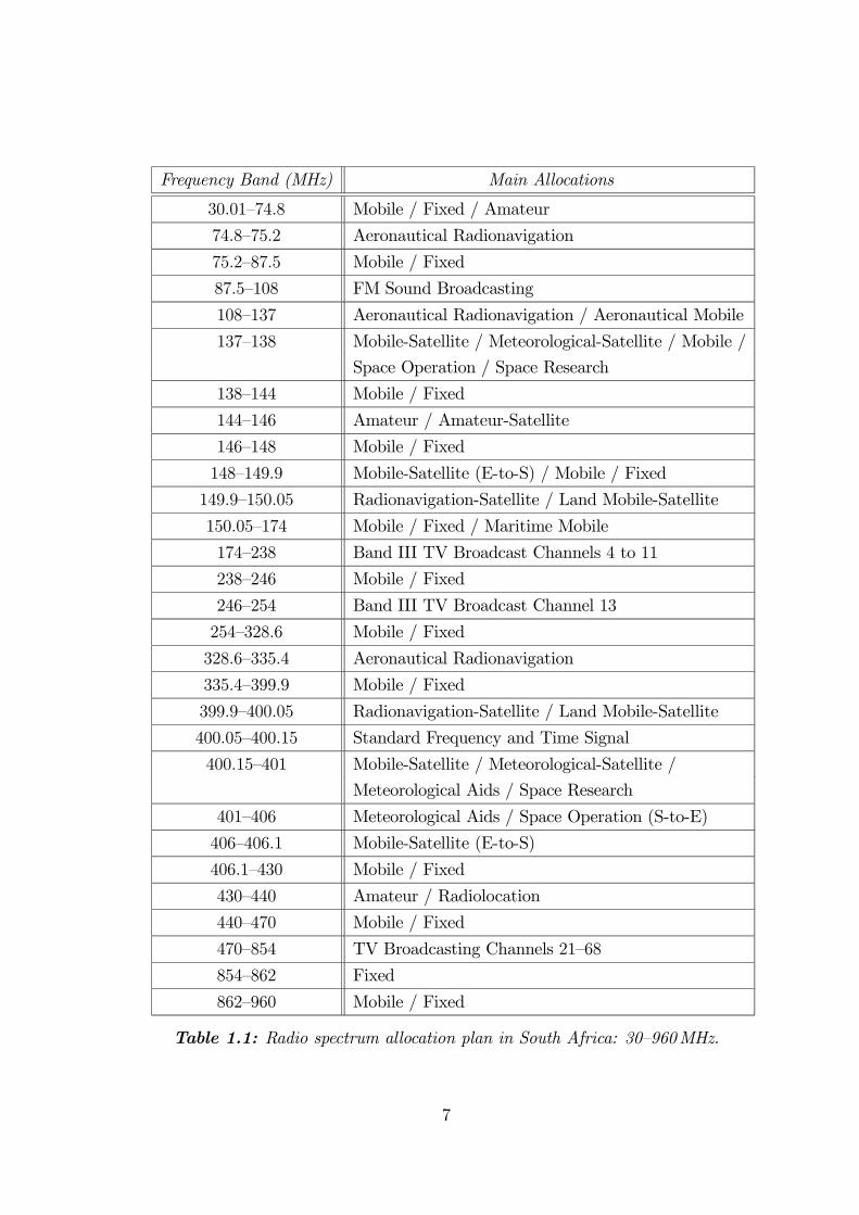
1.1 Radio frequency interference measured in Cape Town: (a) 80—
200MHz; (b) 129—153MHz. . . . . . . . . . . . . . . . . . . . . . 8
1.2 Radio frequency interference measured with the SASAR system
near the Southern Cape, South Africa: (a) H receive polarisation;
(b) V receive polarisation. . . . . . . . . . . . . . . . . . . . . . . 8
1.3 SASAR image of Cape Agulhas before and after radio frequency
interference suppression. The flight path is along the horizontal
axis, with near range towards the bottom of the image. . . . . . . 10
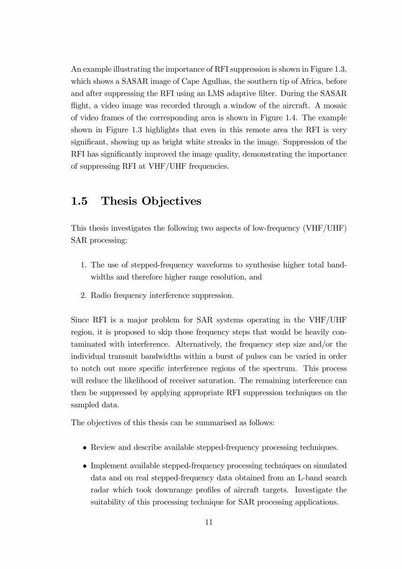
1.4 Mosaic of video frames of the Cape Agulhas area recorded at the
same time as the radar data. . . . . . . . . . . . . . . . . . . . . . 10
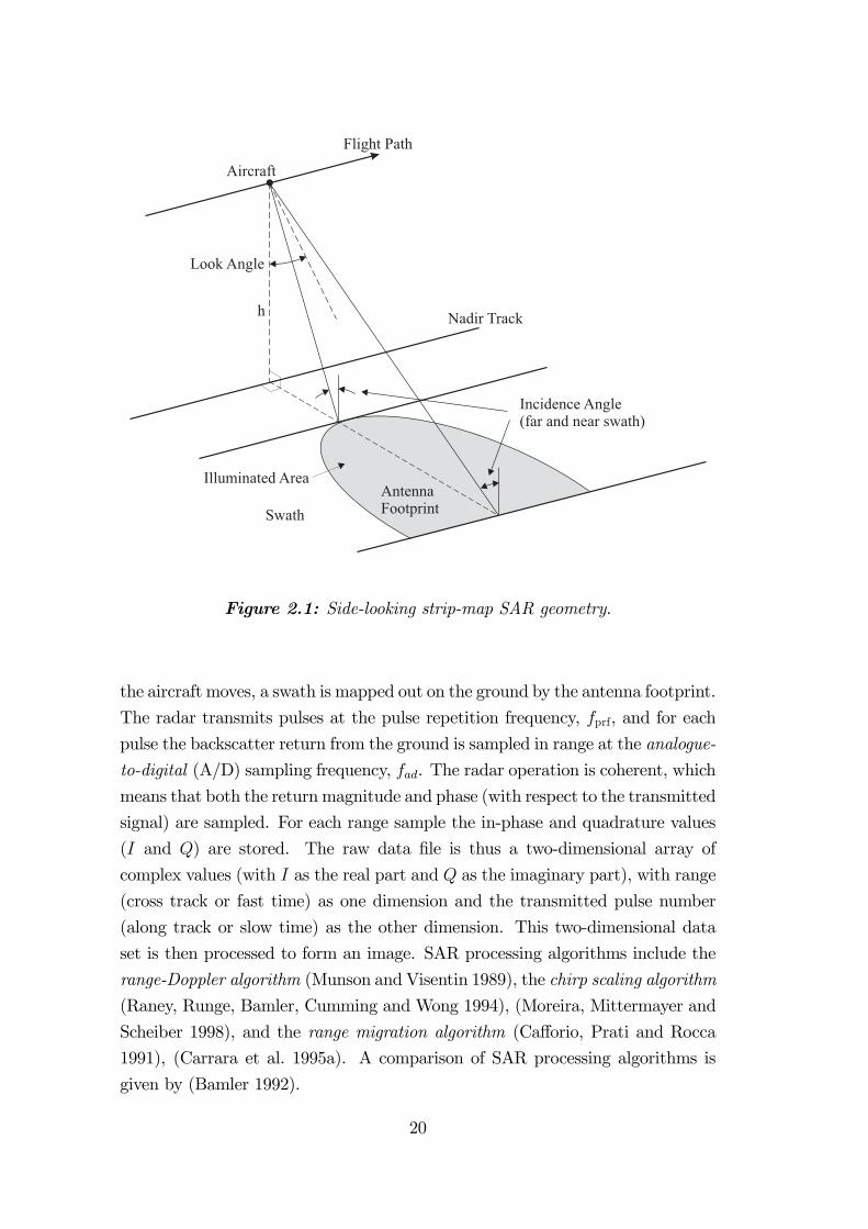
2.1 Side-looking strip-map SAR geometry. . . . . . . . . . . . . . . . 20
2.2 Gap in received data when using multiple receivers. . . . . . . . . 24
2.3 (a) Synthetic range profile of a real Boeing 737; (b) Five adjacent
SRPs of the Boeing, appropriately overlapped. . . . . . . . . . . . 31
2.4 Combination of narrow-bandwidth chirp waveforms to form one
wide-bandwidth chirp waveform. . . . . . . . . . . . . . . . . . . . 33
2.5 Addition of phase-correcting term to narrow-bandwidth signals. . 35
2.6 Simulation results of time-domain method to combine stepped-
frequency waveforms. . . . . . . . . . . . . . . . . . . . . . . . . . 38
2.7 Single-look E-SAR image of Lechfeld, Germany, obtained using
only one frequency step, with Btx = 20MHz. The flight path is
along the vertical axis, with near range towards the left of the image. 40
xi
2.8 Single-look E-SAR image obtained using five frequency steps, with
Bt = 100MHz. . . . . . . . . . . . . . . . . . . . . . . . . . . . . 40
3.1 Reconstruction of target reflectivity spectrum for n = 4 transmit-
ted pulses, each with carrier frequency fi and bandwidth Btx. . . 48
3.2 Construction of compression filter H (f). . . . . . . . . . . . . . . 51
3.3 Stepped-frequency simulation showing the effect when the returned
target spectrum is not bandlimited. . . . . . . . . . . . . . . . . . 55
3.4 Stepped-frequency simulation showing the effect when the returned
target spectrum is bandlimited, and when there is an overlap be-
tween successive subspectra. . . . . . . . . . . . . . . . . . . . . . 56
3.5 Stepped-frequency simulation showing the effect when there is a
gap between successive subspectra. . . . . . . . . . . . . . . . . . 57
3.6 Stepped-frequency simulation showing an example in which one
frequency step has been omitted. . . . . . . . . . . . . . . . . . . 58
3.7 Stepped-frequency simulation showing an example in which dif-
ferent frequency step sizes have been used. . . . . . . . . . . . . . 59
3.8 Stepped-frequency simulation showing an example in which differ-
ent frequency step sizes and different transmit bandwidths have
been used. . . . . . . . . . . . . . . . . . . . . . . . . . . . . . . . 60
3.9 Stepped-frequency simulation using parameters of real aircraft
stepped-frequency data. . . . . . . . . . . . . . . . . . . . . . . . 61
3.10 Stepped-frequency simulation using parameters of real aircraft
stepped-frequency data, without bandlimiting target returns. . . . 62
4.1 (a) RFI measured in Cape Town with a spectrum analyser; (b)
RFI measured with the SASAR system near the Southern Cape,
South Africa. . . . . . . . . . . . . . . . . . . . . . . . . . . . . . 74
4.2 Number of RFI spikes for both H and V polarisation versus power
above noise floor. . . . . . . . . . . . . . . . . . . . . . . . . . . . 75
xii
4.3 P-band image of the vicinity of Weilheim, Germany, degraded by
RF interference. The flight path is along the horizontal axis, with
near range towards the bottom of the image. . . . . . . . . . . . . 77
4.4 STC curve of P-band data. . . . . . . . . . . . . . . . . . . . . . . 79
4.5 Real part of a range line of the P-band data: (a) before STC
removal; (b) after STC removal. . . . . . . . . . . . . . . . . . . . 79
4.6 VHF-band image of the vicinity of Upington, South Africa, de-
graded by RF interference. The flight path is along the horizontal
axis, with near range towards the bottom of the image. . . . . . . 80
4.7 Averaged range spectrum of VHF-band data, showing (a) the
noisy data; (b) the signal envelope obtained using a 33-kernel
median filter; (c) the signal envelope obtained using a 65-kernel
median filter; (d) the signal envelope obtained using a 101-kernel
median filter. . . . . . . . . . . . . . . . . . . . . . . . . . . . . . 82
4.8 Averaged range spectrum of VHF-band data, showing (a) the
noisy data; (b) the signal envelope obtained using a 101-kernel
median filter; (c) the noisy spectrum after subtracting the sig-
nal envelope; (d) the cleaned spectrum after notching out all RFI
spikes more than 3dB above the signal envelope. . . . . . . . . . . 83
4.9 VHF-band image after applying a notch filter to suppress RFI. . . 84
4.10 Optical photo mosaic of VHF-band image. . . . . . . . . . . . . . 84
4.11 Averaged range spectrum of noisy and cleaned VHF-band data. . 85
4.12 The LMS adaptive filter. . . . . . . . . . . . . . . . . . . . . . . . 86
4.13 Simulation results demonstrating the effectiveness of the adaptive
filter when applied to RFI suppression. The three columns show
the ideal, contaminated and cleaned signals respectively. The first
row shows the real part of the signal in the time domain, the
second row shows the signal in the frequency domain, and the
third row shows the range compressed signal. . . . . . . . . . . . . 88
4.14 P-band image after applying the LMS adaptive filter to suppress
RF interference. . . . . . . . . . . . . . . . . . . . . . . . . . . . . 91
xiii

4.15 Averaged range spectrum of noisy and cleaned P-band data. . . . 92
4.16 VHF-band image after applying the LMS adaptive filter to sup-
press RF interference. . . . . . . . . . . . . . . . . . . . . . . . . . 92
4.17 Averaged range spectrum of (a) noisy VHF-band data; (b) cleaned
data using a 64-tap LMS adaptive filter; (c) cleaned data using a
256-tap filter; (d) cleaned data using a 512-tap filter. . . . . . . . 93
4.18 Quality index versus range line. Weight vector is updated (a)
only once; (b) every 2000 range lines; (c) every 500 range lines;
(d) every 100 range lines. . . . . . . . . . . . . . . . . . . . . . . . 97
4.19 Block diagram of LMS adaptive filter with constant tap weights. . 99
4.20 Averaged range spectrum of (a) noisy VHF-band image, and of
cleaned image with weight vector updated every (b) 100, (c) 500
and (d) 1000 range lines. . . . . . . . . . . . . . . . . . . . . . . . 100
4.21 Graphical illustration of sidelobe reduction procedure. The large
triangle represents the wanted compressed target, the small trian-
gle the unwanted sidelobe, and the sinusoidal waveform the un-
wanted RFI interference. . . . . . . . . . . . . . . . . . . . . . . . 101
4.22 Block diagram of sidelobe reduction procedure. . . . . . . . . . . 102
4.23 Simulation results of sidelobe reduction procedure: (a) RFI con-
taminated echo return; (b) filtered echo return with no sidelobe
reduction (arrows point at unwanted sidelobes); (c) filtered echo
return with first-order sidelobe reduction; (d) filtered echo return
with second-order sidelobe reduction. . . . . . . . . . . . . . . . . 103
4.24 P-band data results of sidelobe reduction procedure: (a) RFI con-
taminated image; (b) filtered image without any sidelobe reduc-
tion (the circles indicate regions with very high sidelobes); (c)
filtered image with third-order sidelobe reduction. . . . . . . . . . 105
4.25 VHF-band data results of sidelobe reduction procedure: (a) fil-
tered image without any sidelobe reduction; (b) filtered image
with first-order sidelobe reduction. . . . . . . . . . . . . . . . . . 105
xiv
A.1 Simulation result of IFFT method, with no overlap between suc-
cessive SRPs. See beginning of appendix for details. . . . . . . . . 115
A.2 Simulation result of IFFT method, showing the return from 2
point targets, which are both positioned in one coarse range bin.
See beginning of appendix for details. . . . . . . . . . . . . . . . . 116
A.3 Simulation result of IFFT method, with the 2 point targets being
positioned in neighbouring coarse range bins. See beginning of
appendix for details. . . . . . . . . . . . . . . . . . . . . . . . . . 117
A.4 Simulation result of IFFT method, where the frequency step size
∆f is equal to half the transmitted bandwidth Btx. See beginning
of appendix for details. . . . . . . . . . . . . . . . . . . . . . . . . 118
A.5 Simulation result of IFFTmethod, where the sample frequency fadis equal to twice the transmitted bandwidth Btx. See beginning
of appendix for details. . . . . . . . . . . . . . . . . . . . . . . . . 119
A.6 Simulation result of IFFT method, where the frequency step size
∆f is equal to half the transmitted bandwidthBtx, and the sample
frequency fad is equal to twice the transmitted bandwidthBtx. See
beginning of appendix for details. . . . . . . . . . . . . . . . . . . 120
B.1 High-resolution range profile of a 747 aircraft, processed with the
IFFT method and the spectrum reconstruction method. . . . . . . 122
B.2 High-resolution range profile of an N326 aircraft, processed with
the IFFT method and the spectrum reconstruction method. . . . 123
B.3 High-resolution range profile of a King Air B200 aircraft, processed
with the IFFT method and the spectrum reconstruction method. 124
B.4 High-resolution range profile of aMesser Bolkow aircraft, processed
with the IFFT method and the spectrum reconstruction method. 125
C.1 Cleaned image 1 of Upington area. . . . . . . . . . . . . . . . . . 129
C.2 Cleaned image 2 of Upington area. . . . . . . . . . . . . . . . . . 129
C.3 Correlation image of cleaned datasets. . . . . . . . . . . . . . . . 130
xv
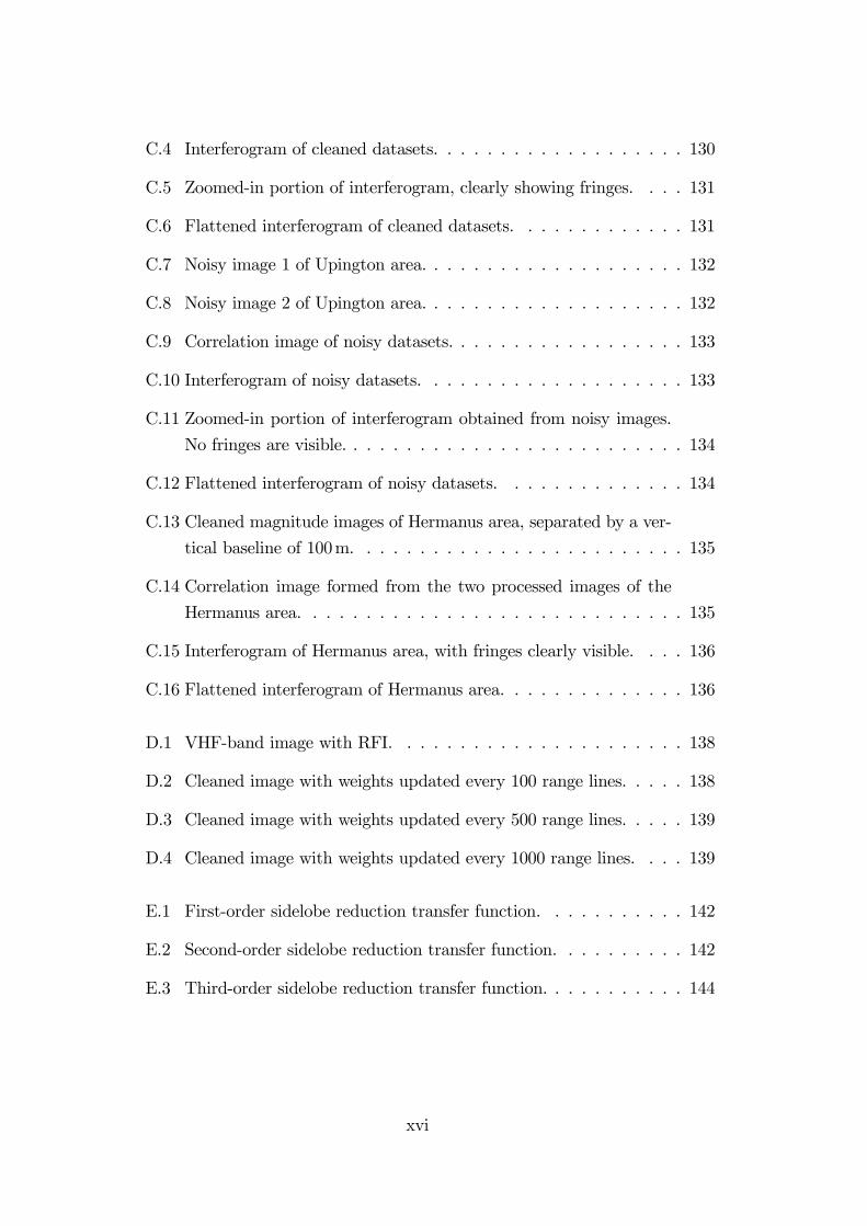
C.4 Interferogram of cleaned datasets. . . . . . . . . . . . . . . . . . . 130
C.5 Zoomed-in portion of interferogram, clearly showing fringes. . . . 131
C.6 Flattened interferogram of cleaned datasets. . . . . . . . . . . . . 131
C.7 Noisy image 1 of Upington area. . . . . . . . . . . . . . . . . . . . 132
C.8 Noisy image 2 of Upington area. . . . . . . . . . . . . . . . . . . . 132
C.9 Correlation image of noisy datasets. . . . . . . . . . . . . . . . . . 133
C.10 Interferogram of noisy datasets. . . . . . . . . . . . . . . . . . . . 133
C.11 Zoomed-in portion of interferogram obtained from noisy images.
No fringes are visible. . . . . . . . . . . . . . . . . . . . . . . . . . 134
C.12 Flattened interferogram of noisy datasets. . . . . . . . . . . . . . 134
C.13 Cleaned magnitude images of Hermanus area, separated by a ver-
tical baseline of 100m. . . . . . . . . . . . . . . . . . . . . . . . . 135
C.14 Correlation image formed from the two processed images of the
Hermanus area. . . . . . . . . . . . . . . . . . . . . . . . . . . . . 135
C.15 Interferogram of Hermanus area, with fringes clearly visible. . . . 136
C.16 Flattened interferogram of Hermanus area. . . . . . . . . . . . . . 136
D.1 VHF-band image with RFI. . . . . . . . . . . . . . . . . . . . . . 138
D.2 Cleaned image with weights updated every 100 range lines. . . . . 138
D.3 Cleaned image with weights updated every 500 range lines. . . . . 139
D.4 Cleaned image with weights updated every 1000 range lines. . . . 139
E.1 First-order sidelobe reduction transfer function. . . . . . . . . . . 142
E.2 Second-order sidelobe reduction transfer function. . . . . . . . . . 142
E.3 Third-order sidelobe reduction transfer function. . . . . . . . . . . 144
xvi
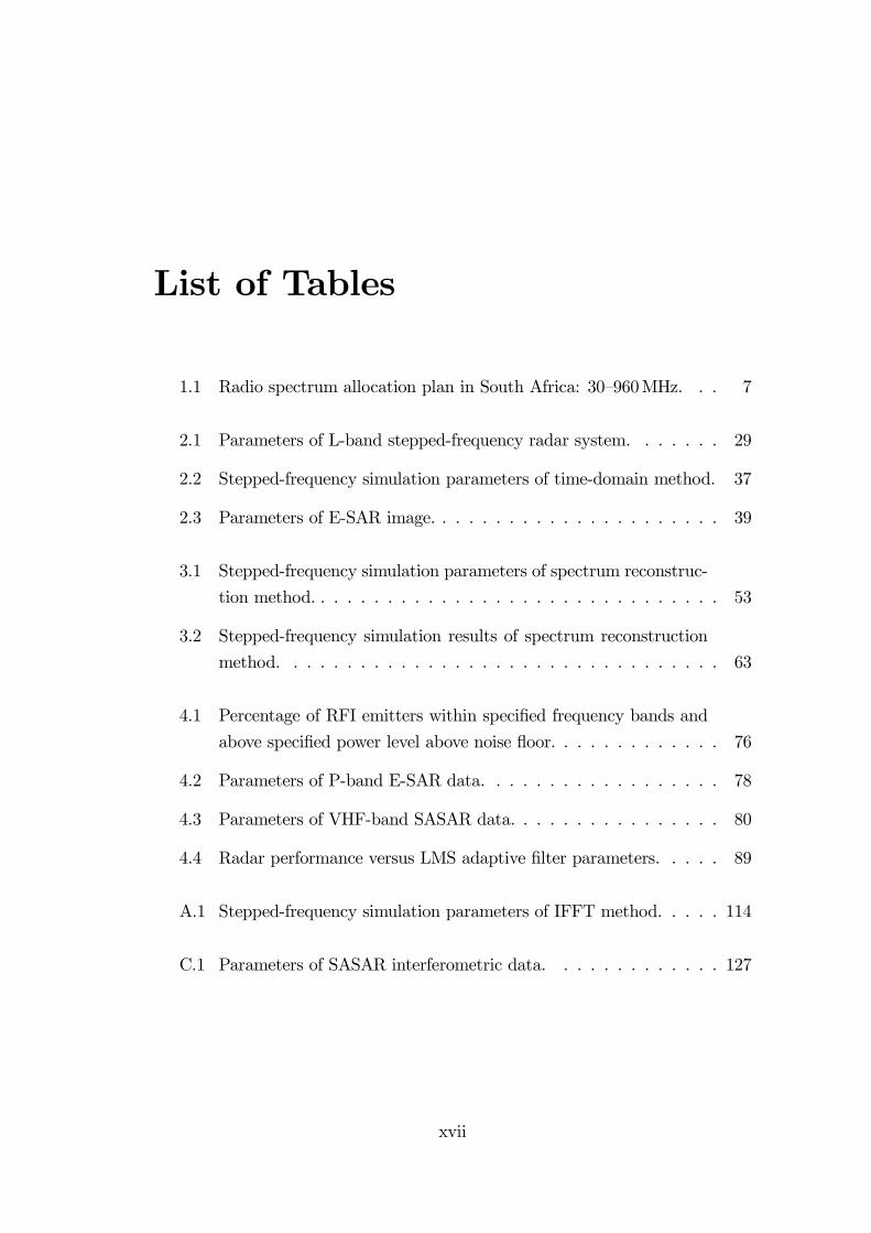
List of Tables
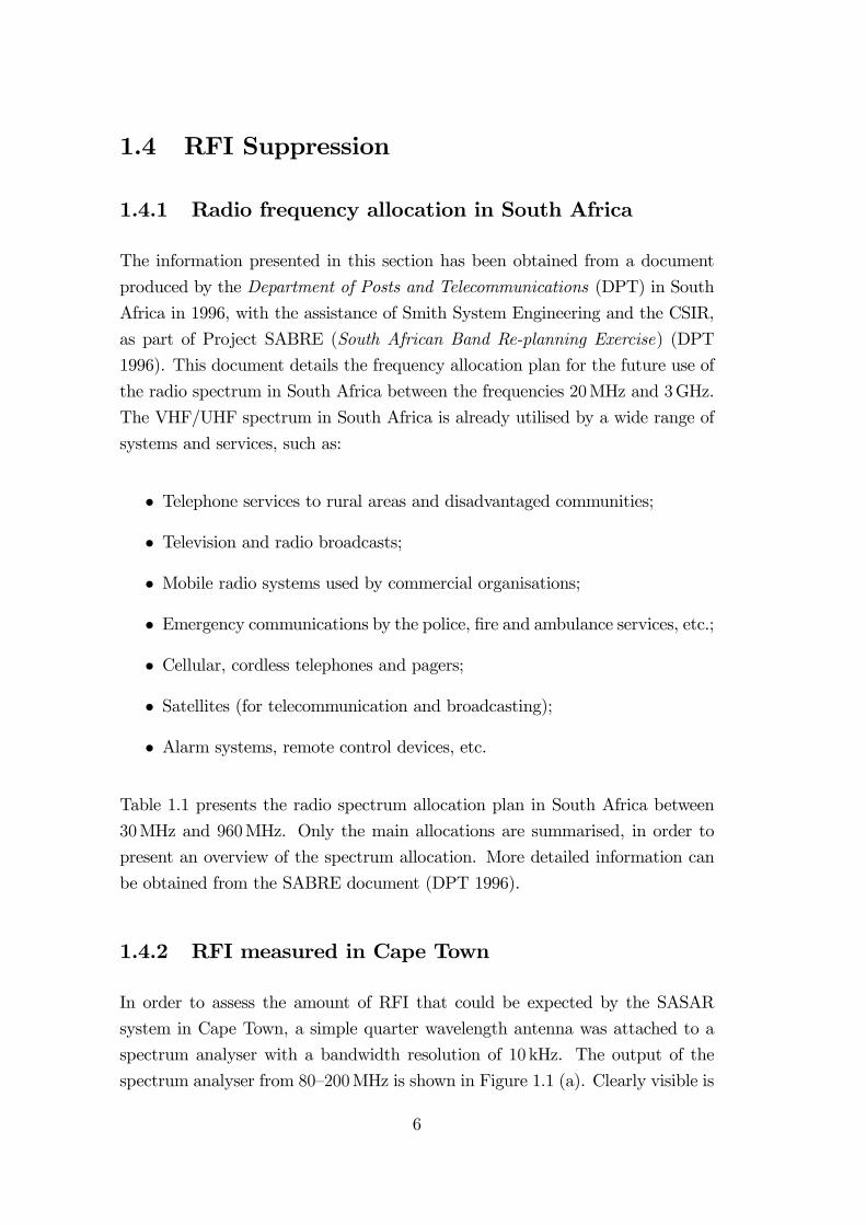
1.1 Radio spectrum allocation plan in South Africa: 30—960MHz. . . 7
2.1 Parameters of L-band stepped-frequency radar system. . . . . . . 29
2.2 Stepped-frequency simulation parameters of time-domain method. 37
2.3 Parameters of E-SAR image. . . . . . . . . . . . . . . . . . . . . . 39
3.1 Stepped-frequency simulation parameters of spectrum reconstruc-
tion method. . . . . . . . . . . . . . . . . . . . . . . . . . . . . . . 53
3.2 Stepped-frequency simulation results of spectrum reconstruction
method. . . . . . . . . . . . . . . . . . . . . . . . . . . . . . . . . 63
4.1 Percentage of RFI emitters within specified frequency bands and
above specified power level above noise floor. . . . . . . . . . . . . 76
4.2 Parameters of P-band E-SAR data. . . . . . . . . . . . . . . . . . 78
4.3 Parameters of VHF-band SASAR data. . . . . . . . . . . . . . . . 80
4.4 Radar performance versus LMS adaptive filter parameters. . . . . 89
A.1 Stepped-frequency simulation parameters of IFFT method. . . . . 114
C.1 Parameters of SASAR interferometric data. . . . . . . . . . . . . 127
xvii

xviii

List of Symbols
A – Amplitude [m]
B – Bandwidth [Hz]
Bd – Doppler bandwidth [Hz]
Bt – Total radar bandwidth [Hz]
Btx – Transmitted RF bandwidth [Hz]
c – Speed of light [m/s]
d – Primary input of LMS adaptive filter
D – Input signal vector
e – Error signal of LMS adaptive filter
f – Frequency [Hz]
fad – Radar A/D sampling frequency [Hz]
fc – Radar centre transmit frequency [Hz]
fc – Centre frequency of reconstructed spectrum [Hz]
fi – Centre frequency of pulse i [Hz]
δfi – Frequency shift associated with pulse i [Hz]
fprf – Pulse repetition frequency [Hz]
∆f – Frequency step size [Hz]
H(f) – Compression filter
H(ω) – Equivalent transfer function of LMS adaptive filter
Ka – Azimuth window broadening constant
Kr – Range window broadening constant
l – Real antenna length [m]
L – Synthetic aperture length [m]
mi – Number of range samples associated with pulse i
M(ω) – Matched filter
n – Number of pulses in a burst of pulses
n(t) – Noise signal
xix

N – Number of filter weights
Pav – Average transmitted power [W]
Ppeak – Peak transmitted power [W]
r – Range [m]
rcoarse – Coarse slant range resolution [m]
rmax – Maximum unambiguous range [m]
rt – Range from radar to target [m]
t – Time [s]
δti – Time shift associated with pulse i [s]
T – Interpulse period [s]
Tp – Pulse length [s]
v – Ground speed [m/s]
v(t) – Range-compressed signal
v (t) – High-resolution, range-compressed signal
vbb(t) – Baseband signal
vrx(t) – Received waveform
vtx(t) – Transmitted waveform
vt – Radial target velocity [m/s]
ws – Synthesised unambiguous range length [m]
W – Weight vector of LMS adaptive filter
x – Reference input of LMS adaptive filter
X – Reference signal vector
y – Output of LMS adaptive filter
Z(f) – Target reflectivity spectrum
γ – Chirp rate of linear FM waveform [Hz/s]
∆ – Delay associated with LMS adaptive filter [s]
ζ(t) – Target reflectivity function
η – Quality index
θs – Squint angle [rad]
λ – Wavelength [m]
λmax – Largest eigenvalue of input correlation matrix
µ – Convergence factor
ρa – Azimuth resolution [m]
∆ρa – Azimuth bin size [m]
ρr – Slant range resolution [m]
∆ρr – Slant range bin size [m]
xx

φi – Phase of pulse i [rad]
∆φ – Phase difference [rad]
ω – Angular frequency [rad/s]
xxi

xxii
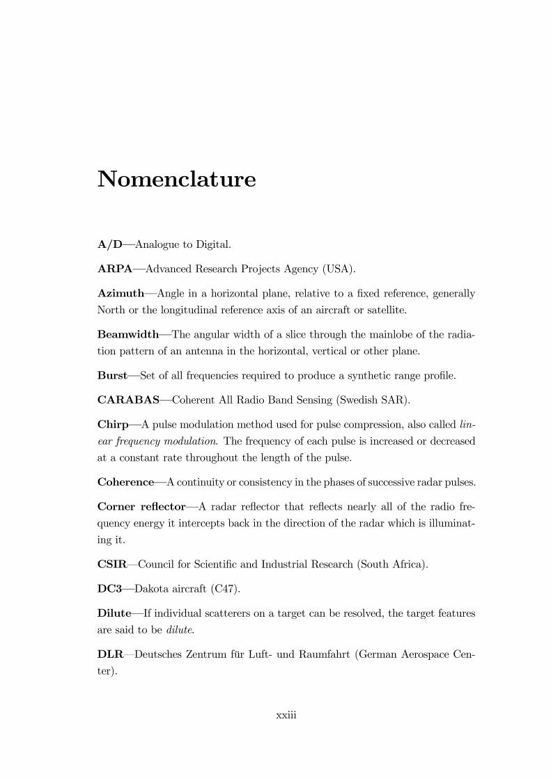
Nomenclature
A/D–Analogue to Digital.
ARPA–Advanced Research Projects Agency (USA).
Azimuth–Angle in a horizontal plane, relative to a fixed reference, generallyNorth or the longitudinal reference axis of an aircraft or satellite.
Beamwidth–The angular width of a slice through the mainlobe of the radia-tion pattern of an antenna in the horizontal, vertical or other plane.
Burst–Set of all frequencies required to produce a synthetic range profile.
CARABAS–Coherent All Radio Band Sensing (Swedish SAR).
Chirp–A pulse modulation method used for pulse compression, also called lin-ear frequency modulation. The frequency of each pulse is increased or decreased
at a constant rate throughout the length of the pulse.
Coherence–A continuity or consistency in the phases of successive radar pulses.
Corner reflector–A radar reflector that reflects nearly all of the radio fre-
quency energy it intercepts back in the direction of the radar which is illuminat-
ing it.
CSIR–Council for Scientific and Industrial Research (South Africa).
DC3–Dakota aircraft (C47).
Dilute–If individual scatterers on a target can be resolved, the target featuresare said to be dilute.
DLR–Deutsches Zentrum für Luft- und Raumfahrt (German Aerospace Cen-
ter).
xxiii
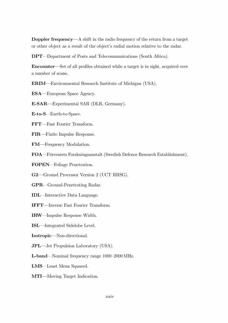
Doppler frequency–A shift in the radio frequency of the return from a targetor other object as a result of the object’s radial motion relative to the radar.
DPT–Department of Posts and Telecommunications (South Africa).
Encounter–Set of all profiles obtained while a target is in sight, acquired overa number of scans.
ERIM–Environmental Research Institute of Michigan (USA).
ESA–European Space Agency.
E-SAR–Experimental SAR (DLR, Germany).
E-to-S–Earth-to-Space.
FFT–Fast Fourier Transform.
FIR–Finite Impulse Response.
FM–Frequency Modulation.
FOA–Försvarets Forskningsanstalt (Swedish Defence Research Establishment).
FOPEN–Foliage Penetration.
G2–Ground Processor Version 2 (UCT RRSG).
GPR–Ground-Penetrating Radar.
IDL–Interactive Data Language.
IFFT–Inverse Fast Fourier Transform.
IRW–Impulse Response Width.
ISL–Integrated Sidelobe Level.
Isotropic–Non-directional.
JPL–Jet Propulsion Laboratory (USA).
L-band–Nominal frequency range 1000—2000MHz.
LMS–Least Mean Squared.
MTI–Moving Target Indication.
xxiv

Nadir–The point directly below the radar platform.
Narrowband–Describes radar systems that transmit and receive waveformswith instantaneous bandwidths less than 1 percent of centre frequency (Taylor
1995).
NAWC–Naval Air Warfare Centre (USA).
NCTR–Non-Co-operative Target Recognition.
PCR–Pulse Compression Ratio.
PRF–Pulse Repetition Frequency.
PRI–Pulse Repetition Interval.
Profile–Contour of the target outline which is deduced from reflected signals
in a radar system.
PSL–Peak Sidelobe Level.
Radar–Radio Detection and Ranging.
Range–The radial distance from a radar to a target.
RFI–Radio Frequency Interference.
RRSG–Radar Remote Sensing Group (UCT).
SAAF–South African Air Force.
SAR–Synthetic Aperture Radar. A signal-processing technique for improvingthe azimuth resolution beyond the beamwidth of the physical antenna actually
used in the radar system. This is done by synthesising the equivalent of a very
long sidelooking array antenna.
SASAR–South African Synthetic Aperture Radar.
Scan–Set of pulses received during illumination time.
SLC–Single Look Complex.
SNR–Signal to Noise Ratio.
Specular–Highly directional. The power returned from a specular reflector
depends very much on the direction of illumination.
xxv
SRP–Synthetic Range Profile.
STC–Sensitivity Time Control.
S-to-E–Space-to-Earth.
Swath–The area on earth illuminated by the antenna signal.
UCT–University of Cape Town (South Africa).
UHF–Ultra High Frequency. Nominal frequency range 300—3000MHz.
UWB–Ultra-Wideband. Describes radar systems that transmit and receivewaveforms with instantaneous bandwidths greater than 25 percent of centre fre-
quency (Taylor 1995).
VHF–Very High Frequency. Nominal frequency range 30—300MHz.
Wideband–Describes radar systems that transmit and receive waveforms withinstantaneous bandwidths between 1 percent and 25 percent of centre frequency
(Taylor 1995).
xxvi
Chapter 1
Introduction
1.1 Background
Synthetic Aperture Radar (SAR) is a technique for creating high resolution im-
ages of the earth’s surface. Over the area of the surface being observed, these
images represent the backscattered microwave energy, which depends on the
properties of the surface, such as its slope, roughness, textural inhomogeneities
and dielectric constant. The radar backscattering cross section also depends
strongly on the existence of vegetation. These dependencies allow SAR imagery
to be used in conjunction with models of the scattering mechanism to measure
various characteristics of the earth’s surface, such as topography.
An important characteristic of SAR is its day/night capability, which it pos-
sesses because it supplies its own illumination and receives the backscatter from
it, as opposed to passive sensors which receive either the earth’s radiation or
the reflected illumination from the sun. Furthermore, a SAR sensor has all-
weather capability, because microwaves propagate through clouds and rain with
only limited attenuation. These features, together with its fine two-dimensional
resolution capability, have made SAR a valuable remote sensing tool for both
military and civilian users. Military SAR applications include intelligence gath-
ering, battlefield reconnaissance and weapons guidance. Civilian applications
include topographic mapping, geology and mining (Lynne and Taylor 1986), oil
spill monitoring (Hovland, Johannessen and Digranes 1994), sea ice monitoring
(Drinkwater, Kwok and Rignot 1990), oceanography (Wahl and Skoelv 1994),
agricultural classification and assessment, land use monitoring and planetary or
celestial investigations (Carrara, Goodman and Majewski 1995a).
1

1.2 Low-Frequency SAR
Increased interest has developed in ultra-wideband VHF/UHF SAR because of
its applications in the areas of foliage penetration radar (FOPEN) and ground-
penetrating radar (GPR) (Elachi, Roth and Schaber 1984), (Berlin, Tarabzouni,
Al-Naser, Sheikho and Larson 1986), (Schaber, McCauley, Breed and Olhoeft
1986). Such applications include the detection of targets concealed by foliage
and/or camouflage (Gustavsson, Flood, Frölind, Hellsten, Jonsson, Larsson,
Stenström and Ulander 1998a), (Gustavsson, Ulander, Flood, Frölind, Hellsten,
Jonsson, Larsson and Stenström 1998b), the detection of buried objects, the de-
tection and location of buried pipes and cables, and archaeological and geological
exploration, such as the location of underground riverbeds (Schaber, Olhoeft and
McCauley 1990). The term ultra-wideband (UWB) describes radar systems that
transmit and receive waveforms with instantaneous bandwidths greater than 25
percent of centre frequency (Taylor 1995). Conventional narrowband radar sys-
tems generally have fractional bandwidths less than 1% of centre frequency, and
wideband radar systems generally have fractional bandwidths from 1% to 25%
of centre frequency.
Airborne SAR sensors which operate below L-band (1000—2000MHz) include:
• The CARABAS-II ultra-wideband VHF SAR system of the Swedish De-
fence Research Establishment (FOA), which operates in the 20—90MHz
region (Larsson, Frölind, Gustavsson, Hellsten, Jonsson, Stenström and
Ulander 1997), (Ulander and Frölind 1999).
• The P-band (450MHz) sensor of the German DLR E-SAR (Buckreuss
1998).
• The NASA/JPL AIRSAR P-band system (http://airsar.jpl.nasa.gov/).
• The NASA/JPL dual-frequency airborne GeoSAR system, which operatesat both P- and X-band (http://lightsar.jpl.nasa.gov/html/projects/geosar/
geosar.html).
• The ARPA/ERIM/NAWC P-3 ultra-wideband SAR, which operates in the215—900MHz region (Carrara, Tummala and Goodman 1995b).
• The Russian iMARK VHF SAR sensor, which has a centre frequency of
120MHz and is operated by the Moscow Scientific Research Institute of
2

Instrument Engineering and the All-Union Scientific Research Institute of
Cosmoaerological Methods.
• The South African SAR (SASAR) VHF sensor which operates with a
12MHz bandwidth centred around 141MHz (Inggs 1996).
The initial design and conception of the SASAR system originated at the Univer-
sity of Cape Town (UCT) (Inggs 1996). Originally it was planned to be a fully
polarimetric, multifrequency SAR system; however, due to budget constraints,
only a single VHF sensor has currently been constructed. The system plat-
form was originally intended to be a Boeing 707 aircraft, offered by the South
African Air Force. However, since the Boeing proved to have limited availabil-
ity, the system is now installed in a South African Airforce DC3/C47 aircraft.
The motivation behind using a VHF sensor is the hope that it will offer unique
opportunities for foliage and ground penetration.
The 12MHz bandwidth of the SASAR system corresponds to a slant range res-
olution of about 12m. It is still hoped to increase the resolution to about 1.5m,
which would require a total bandwidth of 100MHz. For SAR systems operating
in the VHF/UHF-band, this bandwidth would be a large fraction of the transmit
centre frequency and would be more difficult to obtain than for systems operating
at C- or X-band. The most difficult problem when implementing a large frac-
tional bandwidth system is the design of a broad-band antenna. However, one
possible method of achieving this bandwidth would be to use stepped-frequency
waveforms.
1.3 Motivation for Using Stepped-Frequency
Waveforms
1.3.1 Achieving higher total bandwidth
The total radar bandwidth of a stepped-frequency system is synthetically ob-
tained by combining a burst of narrow-bandwidth returns through the appli-
cation of a signal processing method. Stepped-frequency processing therefore
offers the possibility of economically upgrading an existing single frequency SAR
system to improve its bandwidth and therefore its range resolution, since only
3
minimal modifications to the existing radar system are required. Although this
thesis is only concerned with the signal processing aspect of a stepped-frequency
system and not with the system level design of such a system, the following two
main steps for such an upgrade are noted:
1. The design of a broader band antenna, which is capable of transmitting and
receiving the entire required frequency range. If the bandwidth increase is
not too large, the existing antenna might even be sufficient in some cases.
2. The employment of a frequency synthesizer, which steps through the entire
frequency range. It would not be necessary to modify the existing chirp
waveform generator.
Since the instantaneous bandwidth received at the radar is only a fraction of the
total synthesised bandwidth, there is also no need to upgrade the existing A/D
converters. It is also easier to switch between modes of different resolutions,
without paying the penalty of receiving increased amounts of radio frequency
interference (RFI) due to having a wide-bandwidth receiver. These aspects make
the design of a stepped-frequency SAR system economically attractive and viable.
1.3.2 Higher receiver dynamic range
Another advantage of having A/D converters which need only sample at a lower
rate because of the lower instantaneous bandwidth is the ability to sample with
a larger number of bits, because there is a trade-off between sampling frequency
and number of sampling bits. Sampling with a larger number of bits increases the
receiver dynamic range, which is an important consideration for low-frequency
SAR, since the RFI encountered in the VHF/UHF-band (such as FM-radio or
TV) is often many tens of dB stronger than the signal. Increasing the receiver
dynamic range reduces the possibility of receiver saturation. Receiver saturation
causes clipping of the received signal and signal suppression, which degrades the
image quality and leads to the formation of higher harmonics, making the task
of interference suppression algorithms more demanding. According to Ulander
(Ulander 1998), the receiver dynamic range required for wide-beam and ultra-
wideband SAR in the VHF-band (such as the CARABAS-II SAR system) is
typically of the order of 80dB. However, this dynamic range can be achieved
4
only by sacrificing bandwidth. State-of-the-art receiver technology can typically
only achieve a bandwidth of about 10MHz or less with a spurious-free dynamic
range of 80dB (Ulander 1998). Stepped-frequency SAR processing therefore
offers a way to design wideband SAR systems which also have the required high
receiver dynamic range at VHF/UHF frequencies.
1.3.3 Radio frequency interference suppression
Unfortunately, from the point of view of SAR implementations, the VHF/UHF
portion of the spectrum is already in heavy use by other services, such as tele-
vision, mobile communications, radio and cellular phones. Even in remote loca-
tions the interference power often exceeds receiver noise by many dB, becoming
the limiting factor on system sensitivity and severely degrading the image qual-
ity. Therefore it is important to investigate possible means of suppressing the
interference in the received signal.
When the bandwidth of an existing SAR system is increased, the situation de-
generates further, since the radar becomes susceptible to receiver saturation over
that whole band. Given the large number of narrowband interfering sources,
interference vectors may sporadically combine constructively, increasing the in-
stantaneous magnitude of the interference, and thereby increasing the likelihood
of receiver saturation even more.
In order to alleviate the problem of receiver saturation, it is proposed in this thesis
to use stepped-frequency waveforms to avoid regions in the frequency spectrum
that contain the dominant interfering sources. This can be achieved by sim-
ply omitting the relevant frequency steps when sweeping through the frequency
range. These frequency “holes” will, however, raise the sidelobes. A more sophis-
ticated method would be to change adaptively the frequency step size, or even
the transmit bandwidth, in order to notch out as little spectrum as possible. Ide-
ally the transmitter should be switched off occasionally, in order to receive only
interference or so-called “sniffer” pulses. This data could then be used to decide
which regions in the spectrum should be avoided because of strong interference.
Alternatively, a study of the local interference environment could be carried out
in order to decide in advance which spectral regions to avoid. A more detailed
description of the interference environment encountered in South Africa is given
in Section 1.4.
5
1.4 RFI Suppression
1.4.1 Radio frequency allocation in South Africa
The information presented in this section has been obtained from a document
produced by the Department of Posts and Telecommunications (DPT) in South
Africa in 1996, with the assistance of Smith System Engineering and the CSIR,
as part of Project SABRE (South African Band Re-planning Exercise) (DPT
1996). This document details the frequency allocation plan for the future use of
the radio spectrum in South Africa between the frequencies 20MHz and 3GHz.
The VHF/UHF spectrum in South Africa is already utilised by a wide range of
systems and services, such as:
• Telephone services to rural areas and disadvantaged communities;
• Television and radio broadcasts;
• Mobile radio systems used by commercial organisations;
• Emergency communications by the police, fire and ambulance services, etc.;
• Cellular, cordless telephones and pagers;
• Satellites (for telecommunication and broadcasting);
• Alarm systems, remote control devices, etc.
Table 1.1 presents the radio spectrum allocation plan in South Africa between
30MHz and 960MHz. Only the main allocations are summarised, in order to
present an overview of the spectrum allocation. More detailed information can
be obtained from the SABRE document (DPT 1996).
1.4.2 RFI measured in Cape Town
In order to assess the amount of RFI that could be expected by the SASAR
system in Cape Town, a simple quarter wavelength antenna was attached to a
spectrum analyser with a bandwidth resolution of 10kHz. The output of the
spectrum analyser from 80—200MHz is shown in Figure 1.1 (a). Clearly visible is
6
Frequency Band (MHz) Main Allocations
30.01—74.8 Mobile / Fixed / Amateur
74.8—75.2 Aeronautical Radionavigation
75.2—87.5 Mobile / Fixed
87.5—108 FM Sound Broadcasting
108—137 Aeronautical Radionavigation / Aeronautical Mobile
137—138 Mobile-Satellite / Meteorological-Satellite / Mobile /
Space Operation / Space Research
138—144 Mobile / Fixed
144—146 Amateur / Amateur-Satellite
146—148 Mobile / Fixed
148—149.9 Mobile-Satellite (E-to-S) / Mobile / Fixed
149.9—150.05 Radionavigation-Satellite / Land Mobile-Satellite
150.05—174 Mobile / Fixed / Maritime Mobile
174—238 Band III TV Broadcast Channels 4 to 11
238—246 Mobile / Fixed
246—254 Band III TV Broadcast Channel 13
254—328.6 Mobile / Fixed
328.6—335.4 Aeronautical Radionavigation
335.4—399.9 Mobile / Fixed
399.9—400.05 Radionavigation-Satellite / Land Mobile-Satellite
400.05—400.15 Standard Frequency and Time Signal
400.15—401 Mobile-Satellite / Meteorological-Satellite /
Meteorological Aids / Space Research
401—406 Meteorological Aids / Space Operation (S-to-E)
406—406.1 Mobile-Satellite (E-to-S)
406.1—430 Mobile / Fixed
430—440 Amateur / Radiolocation
440—470 Mobile / Fixed
470—854 TV Broadcasting Channels 21—68
854—862 Fixed
862—960 Mobile / Fixed
Table 1.1: Radio spectrum allocation plan in South Africa: 30—960MHz.
7
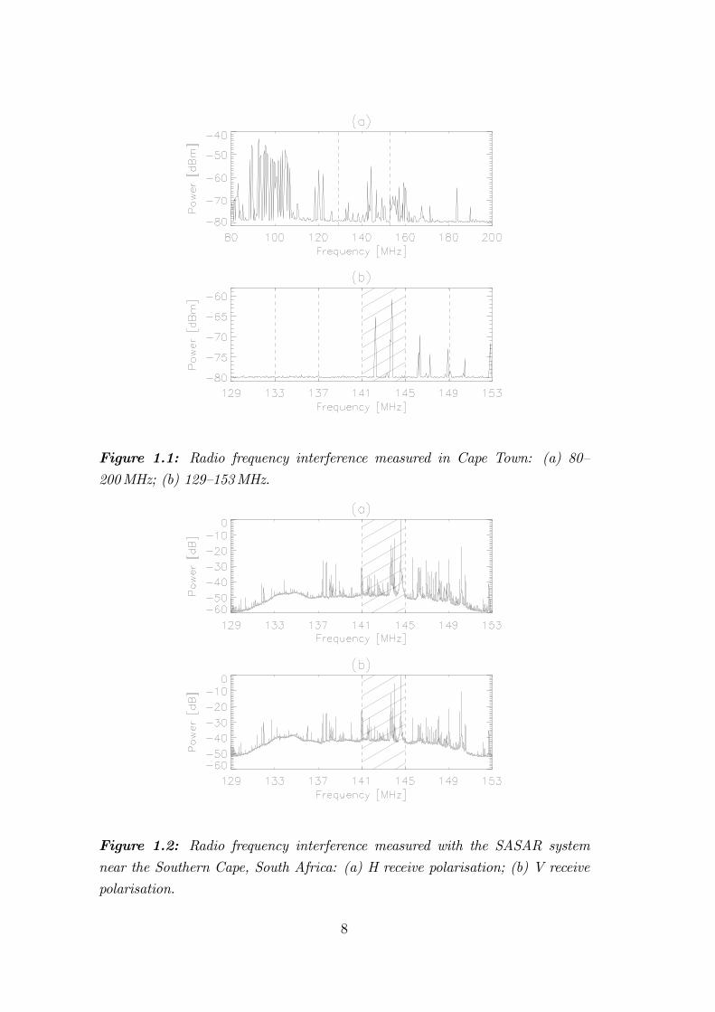
Figure 1.1: Radio frequency interference measured in Cape Town: (a) 80—200MHz; (b) 129—153MHz.
Figure 1.2: Radio frequency interference measured with the SASAR system
near the Southern Cape, South Africa: (a) H receive polarisation; (b) V receive
polarisation.
8
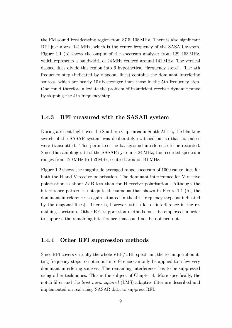
the FM sound broadcasting region from 87.5—108MHz. There is also significant
RFI just above 141MHz, which is the centre frequency of the SASAR system.
Figure 1.1 (b) shows the output of the spectrum analyser from 129—153MHz,
which represents a bandwidth of 24MHz centred around 141MHz. The vertical
dashed lines divide this region into 6 hypothetical “frequency steps”. The 4th
frequency step (indicated by diagonal lines) contains the dominant interfering
sources, which are nearly 10dB stronger than those in the 5th frequency step.
One could therefore alleviate the problem of insufficient receiver dynamic range
by skipping the 4th frequency step.
1.4.3 RFI measured with the SASAR system
During a recent flight over the Southern Cape area in South Africa, the blanking
switch of the SASAR system was deliberately switched on, so that no pulses
were transmitted. This permitted the background interference to be recorded.
Since the sampling rate of the SASAR system is 24MHz, the recorded spectrum
ranges from 129MHz to 153MHz, centred around 141MHz.
Figure 1.2 shows the magnitude averaged range spectrum of 1000 range lines for
both the H and V receive polarisation. The dominant interference for V receive
polarisation is about 5dB less than for H receive polarisation. Although the
interference pattern is not quite the same as that shown in Figure 1.1 (b), the
dominant interference is again situated in the 4th frequency step (as indicated
by the diagonal lines). There is, however, still a lot of interference in the re-
maining spectrum. Other RFI suppression methods must be employed in order
to suppress the remaining interference that could not be notched out.
1.4.4 Other RFI suppression methods
Since RFI covers virtually the whole VHF/UHF spectrum, the technique of omit-
ting frequency steps to notch out interference can only be applied to a few very
dominant interfering sources. The remaining interference has to be suppressed
using other techniques. This is the subject of Chapter 4. More specifically, the
notch filter and the least mean squared (LMS) adaptive filter are described and
implemented on real noisy SASAR data to suppress RFI.
9
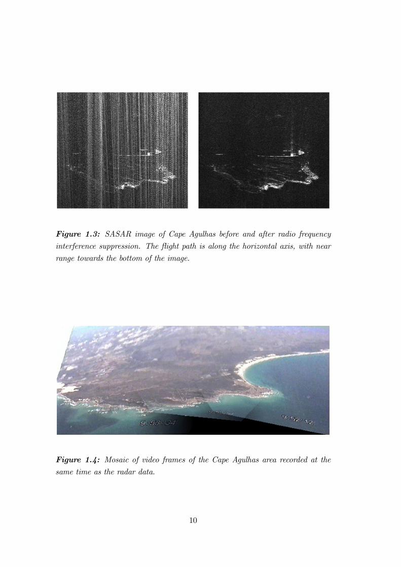
Figure 1.3: SASAR image of Cape Agulhas before and after radio frequency
interference suppression. The flight path is along the horizontal axis, with near
range towards the bottom of the image.
Figure 1.4: Mosaic of video frames of the Cape Agulhas area recorded at thesame time as the radar data.
10
An example illustrating the importance of RFI suppression is shown in Figure 1.3,
which shows a SASAR image of Cape Agulhas, the southern tip of Africa, before
and after suppressing the RFI using an LMS adaptive filter. During the SASAR
flight, a video image was recorded through a window of the aircraft. A mosaic
of video frames of the corresponding area is shown in Figure 1.4. The example
shown in Figure 1.3 highlights that even in this remote area the RFI is very
significant, showing up as bright white streaks in the image. Suppression of the
RFI has significantly improved the image quality, demonstrating the importance
of suppressing RFI at VHF/UHF frequencies.
1.5 Thesis Objectives
This thesis investigates the following two aspects of low-frequency (VHF/UHF)
SAR processing:
1. The use of stepped-frequency waveforms to synthesise higher total band-
widths and therefore higher range resolution, and
2. Radio frequency interference suppression.
Since RFI is a major problem for SAR systems operating in the VHF/UHF
region, it is proposed to skip those frequency steps that would be heavily con-
taminated with interference. Alternatively, the frequency step size and/or the
individual transmit bandwidths within a burst of pulses can be varied in order
to notch out more specific interference regions of the spectrum. This process
will reduce the likelihood of receiver saturation. The remaining interference can
then be suppressed by applying appropriate RFI suppression techniques on the
sampled data.
The objectives of this thesis can be summarised as follows:
• Review and describe available stepped-frequency processing techniques.
• Implement available stepped-frequency processing techniques on simulateddata and on real stepped-frequency data obtained from an L-band search
radar which took downrange profiles of aircraft targets. Investigate the
suitability of this processing technique for SAR processing applications.
11

• Develop an alternative method of processing stepped-frequency data, whichis more suitable for SAR processing applications.
• Implement this method on simulated data, showing how this technique maybe used to avoid spectral regions which are heavily contaminated with RFI.
• Review available RFI suppression techniques and implement a suitable
method to suppress RFI.
• Apply this method on simulated data, on real P-band data generated bythe experimental airborne SAR system E-SAR of the DLR, and on real
VHF-band data generated by the South African SAR (SASAR) system.
• Investigate means to implement the RFI suppression algorithm more ef-
ficiently and to combat unwanted sidelobes that might arise due to the
suppression algorithm.
1.6 Thesis Development
Chapter 2 reviews relevant SAR theory and describes the concept of range res-
olution. It is shown how stepped-frequency waveforms may be used as a means
of synthetically increasing the total radar bandwidth, thereby increasing the
range resolution. Stepped-frequency waveforms also provide opportunities for
RFI suppression by avoiding spectral regions that contain strong interferers, and
they also help to increase the receiver dynamic range, because the task of the
A/D converters is less demanding since they only have to sample the narrowband
pulses.
After motivating the use of stepped-frequency waveforms, three methods of
processing stepped-frequency waveforms are described, namely:
• An IFFT method;
• A time-domain method;
• A frequency-domain method.
The IFFT method is successfully used to obtain high resolution synthetic down-
range profiles of targets such as aircraft. Simulation results are shown, as well
12
as results processed from real stepped-frequency data obtained from an L-band
search radar taking downrange profiles of aircraft targets. Although successful
results have been obtained, this technique has the drawback that target energy
spills over into consecutive coarse range bins, leading to multiple instances of
the target (also called “ghost targets”) in neighbouring coarse range bins. This
drawback makes this method unsuitable for SAR processing purposes.
The time-domain technique involves the reconstruction of a wideband chirp wave-
form from an ensemble of narrowband chirp waveforms stepped in frequency. It
is implemented on simulated data and on real E-SAR data. This technique is,
however, inefficient, mainly due to the upsampling requirement of the narrow-
bandwidth signals.
The inefficiencies of the time-domain technique have, in part, led to the devel-
opment of a more efficient frequency-domain technique. This technique involves
the reconstruction of a wider portion of the target’s reflectivity spectrum by
combining the individual spectra of the transmitted narrow-bandwidth pulses in
the frequency domain.
Chapter 3 describes the frequency-domain approach of processing stepped-frequen-
cy data in more detail. The technique is verified and illustrated by implementing
it on simulated data. It is shown how this technique may be used to avoid spe-
cific spectral regions contaminated with RFI. The remainder of the interference
can then be suppressed by a suitable RFI suppression technique.
Chapter 4 describes and discusses several RFI suppression methods. These in-
clude spectral estimation and coherent subtraction algorithms and various filter
approaches. The notch filter and the LMS adaptive filter are implemented on
P-band data obtained from the DLR, as well as on VHF-band data obtained
from the locally-built SASAR system.
A quality index is defined to monitor the performance of the LMS adaptive filter.
This index is employed to validate the use of the same set of filter tap weights
for many successive range lines. It is explained how the equivalent transfer
function of the LMS adaptive filter may be obtained and combined with the
matched filter transfer function of the range compression stage of the range-
Doppler SAR processing algorithm. Since the equivalent transfer function of the
RFI suppression stage is often effective for hundreds of range lines, significant
computational savings can be achieved.
13
There is discussion of a technique that has been developed to reduce the side-
lobes that appear as an unwanted by-product when the LMS adaptive filter is
used to suppress RFI. The sidelobe reduction procedure can be written in terms
of the equivalent transfer function of the LMS adaptive filter. Thus, a combined
transfer function can be obtained which implements RFI suppression, sidelobe
reduction and range compression simultaneously, thereby leading to a very effi-
cient implementation.
Chapter 5 summarises the work and gives recommendations for future research.
1.7 Statement of Originality
The candidate’s original contributions in this thesis are summarised as follows:
Chapter 2 (Obtaining High Resolution from Narrowband Stepped-Frequency
Pulses) – This chapter describes three methods of processing stepped-frequency
data, namely an IFFT method, a time-domain method and a frequency-domain
method.
The IFFT method is described and implemented on simulated data and on real
data. Both the simulation results and the results from an L-band search radar
taking downrange profiles of aircraft targets have been used to show that this
method is not suitable for SAR processing applications. The description of the
limitations of the IFFT approach for SAR processing applications has not been
documented in the literature. Furthermore, the coding and the implementation
of the IFFT method on stepped-frequency data are the candidate’s own work.
The time-domain technique for processing stepped-frequency data was developed
entirely by the candidate. However, this approach, which involves the recon-
struction of a wideband chirp waveform from an ensemble of narrowband chirp
waveforms stepped in frequency, is shown to be inefficient, mainly because the
narrow-bandwidth signals need to be upsampled.
The frequency-domain approach involves the reconstruction of a wider portion
of the target’s reflectivity spectrum by combining the individual spectra of the
transmitted narrow-bandwidth pulses in the frequency domain. The concept and
mathematical modelling of reconstructing a target’s reflectivity spectrum was
suggested to the candidate by Andrew Wilkinson (Wilkinson 1996). A similar
14
technique, based on the same principle, has been developed independently by the
CARABAS group (Ulander and Frölind 1999). To the best of the candidate’s
knowledge, however, the concept of describing this technique in terms of the
target reflectivity profile is novel.
Chapter 3 (Reconstruction of Target Reflectivity Spectrum) – This chapter de-
scribes the frequency-domain approach of processing stepped-frequency data in
more detail. The technique is verified and illustrated by implementing it on
simulated data. The concept of skipping frequencies which would otherwise be
corrupted by RFI has not been documented in the literature. It is shown that
both the frequency step sizes and the individual transmit bandwidths within a
burst of pulses can be varied. This offers more flexibility in notching out specific
regions of the spectrum which contain dominant interferers. The candidate is
indebted to Andrew Wilkinson (RRSG, UCT) for the mathematical modelling
and description of this technique (Wilkinson 1996). Only the coding and imple-
mentation of this method on simulated data are the candidate’s own work.
Chapter 4 (RFI Suppression for VHF/UHF SAR) – The candidate has been
involved extensively with the RFI suppression aspect of the SASAR system.
Apart from assessing the suitability of the notch filter and the least-mean-squared
(LMS) adaptive filter to suppress RFI in P-band and VHF-band images, original
contributions of this chapter include modifications to these filters in order to
enhance their performance. These modifications involve the use of a median
filter to obtain an approximation of the signal spectrum envelope, which is then
used by the notch filter to identify and remove interference spikes. Furthermore,
the notch filter has been efficiently integrated with the range-compression stage
of the range-Doppler SAR processor.
Modifications to the LMS adaptive filter include sweeping the filter through each
range line from both ends and then averaging the two outputs, sweeping the filter
through each range line twice to allow better convergence of the weight vector,
and zero-padding each range line to reduce edge effects. The issue of finding
optimal filter parameters is discussed, as well as the issue of whether the same
filter tap weights may be used over many successive range lines.
More novel work concerning the LMS adaptive filter includes re-writing it in
terms of an equivalent transfer function, which facilitates efficient integration
with the range-Doppler algorithm. Furthermore, a novel technique is described
15

to reduce range sidelobes, which arise as an unwanted by-product of the RFI
suppression stage. It is shown that the interference suppression and the side-
lobe reduction can be integrated with the range-compression stage of the range-
Doppler algorithm, thereby resulting in a very efficient implementation. The
development, coding, simulation and testing of both the notch filter and the
LMS adaptive filter is the candidate’s own work.
16
Chapter 2
Obtaining High Resolution fromNarrowband Stepped-FrequencyPulses
2.1 Introduction
This chapter introduces the concept of side-looking strip-map SAR in Section 2.2
and briefly describes the steps involved to form a two-dimensional SAR image.
An important characteristic of a SAR image is its resolution, which is defined in
terms of the minimum distance at which two closely spaced scatterers of equal
strength may be resolved. The concept of range resolution, which is the resolu-
tion in the cross track dimension, is described in Section 2.3. It is shown that the
range resolution of a SAR system is directly dependent on the transmitted band-
width, which may be synthetically increased by utilising stepped-frequency wave-
forms. Section 2.4 describes some of the implications of using stepped-frequency
waveforms, such as the increase of the pulse repetition frequency (PRF), velocity
compensation and motion compensation.
In order to obtain the high-resolution range profile from a burst of narrowband
pulses stepped in frequency, some kind of signal processing has to be performed on
the data. This chapter describes two methods of processing stepped-frequency
waveforms so as to produce high-resolution range profiles known as synthetic
range profiles (SRPs) (Wehner 1995), namely:
1. An IFFT method;
2. A time-domain method.
17

Both of these methods are shown to be either unsuitable or too inefficient for
SAR processing applications. Chapter 3 describes a further method of processing
stepped-frequency waveforms which does not suffer from the drawbacks of the
two methods described in this chapter.
The IFFT method involves taking an inverse FFT of the sampled stepped-
frequency data, and is described in detail by (Wehner 1995), (Scheer and Kurtz
1993) and (Currie and Brown 1987). A brief description of this method is given in
Section 2.5, and Section 2.5.2 describes simulation results. Section 2.5.3 describes
the results obtained from implementing this method on real stepped-frequency
data obtained from an L-band search radar taking downrange profiles of aircraft
targets. This work was part of a non-cooperative target recognition (NCTR)
project carried out at the University of Cape Town (UCT) (Lengenfelder 1998a).
The simulation results and the experience gained from processing the aircraft
data have shown that the IFFT method is unsuitable for processing SAR im-
ages, mainly because of the spill-over effect due to matched filtering, which causes
multiple “ghost” images to appear in the final range profile. Original contribu-
tions contained in this section include an analysis of the practical experience
gained from applying this method to real stepped-frequency aircraft data, and
the illustration of the shortcomings of this method as it pertains to SAR process-
ing applications. The coding and the implementation of the IFFT method on
stepped-frequency data is the candidate’s own work. Some of the material in this
section has been published in the Proceedings of IGARSS’96 (Lord and Inggs
1996).
The time-domain technique for combining stepped-frequency waveforms to pro-
duce high-resolution synthetic range profiles does not suffer from the “ghost-
target” drawback and is thus more suitable for SAR processing applications.
It involves the reconstruction of a wideband chirp waveform from the ensemble
of narrowband chirp waveforms stepped in frequency and is described in Sec-
tion 2.6. All the signal processing operations are performed in the time-domain.
It is shown that this method is inefficient mainly on account of the upsampling re-
quirement of the narrow-bandwidth signals. However, it is nevertheless included
in this thesis because it does present a novel and feasible method for combining
stepped-frequency waveforms to process SAR images and because it is perhaps
useful for time-domain SAR processors. Results obtained from processing simu-
lated data and real E-SAR data are presented and discussed. Some of the work
18

described in this section has been published in the Proceedings of IGARSS’97
(Lord and Inggs 1997b) and in the Proceedings of COMSIG’97 (Lord and Inggs
1997a).
The methods described in this chapter adopt the start-stop approximation, which
means that the radar-target range remains constant during the transmission of
one burst of frequencies. It is assumed that the entire sub-band signals are col-
lected before the aircraft moves by half of the antenna size. This ensures that the
largest Doppler variation among all sub-band signals will be small. Although az-
imuth compression and range curvature correction are essential for obtaining high
resolution SAR images, this thesis is only concerned with the issue of obtaining
high range resolutions. Motion compensation is another important consideration
for airborne SAR systems, but is only briefly discussed in Section 2.4.3. Another
problem not discussed at all in this thesis is the variation of the radar response
with frequency and observation angle (Axelsson 1995), which varies significantly
over the synthetic aperture path.
2.2 Side-Looking Strip-Map SAR
An intuitive introduction to basic SAR theory is given by (Stimson 1983). More
advanced treatments on basic SAR theory are provided by (Vant 1989), (Kirk
1975), (Sack, Ito and Cumming 1985) and (Munson and Visentin 1989). A the-
oretical basis for understanding SAR images is provided by (Oliver and Quegan
1998). Other texts with a treatment of SAR theory are offered by (Curlander
and McDonough 1991), (Skolnik 1990), (Elachi 1988) and (Fitch 1988).
The data for a SAR image is collected by an aircraft or satellite with a side-
looking antenna, which transmits a stream of radar pulses and records the
backscattered signal corresponding to each pulse. The rate or pulse repetition
frequency (PRF) at which pulses are transmitted and received may be constant
or may vary over time. Varying the PRF allows the system to maintain a con-
stant spatial distance between pulses if the sensor velocity changes. Since the
moving antenna beam covers a strip of the earth’s surface, this type of SAR
imaging is referred to as strip-map SAR.
Figure 2.1 shows the strip-map SAR geometry. The radar antenna is pointed to
the side of the aircraft towards the ground and orthogonal to the flight track. As
19
Flight Path
Look Angle
hNadir Track
Illuminated Area
Aircraft
AntennaFootprintSwath
Incidence Angle(far and near swath)
Figure 2.1: Side-looking strip-map SAR geometry.
the aircraft moves, a swath is mapped out on the ground by the antenna footprint.
The radar transmits pulses at the pulse repetition frequency, fprf, and for each
pulse the backscatter return from the ground is sampled in range at the analogue-
to-digital (A/D) sampling frequency, fad. The radar operation is coherent, which
means that both the return magnitude and phase (with respect to the transmitted
signal) are sampled. For each range sample the in-phase and quadrature values
(I and Q) are stored. The raw data file is thus a two-dimensional array of
complex values (with I as the real part and Q as the imaginary part), with range
(cross track or fast time) as one dimension and the transmitted pulse number
(along track or slow time) as the other dimension. This two-dimensional data
set is then processed to form an image. SAR processing algorithms include the
range-Doppler algorithm (Munson and Visentin 1989), the chirp scaling algorithm
(Raney, Runge, Bamler, Cumming and Wong 1994), (Moreira, Mittermayer and
Scheiber 1998), and the range migration algorithm (Cafforio, Prati and Rocca
1991), (Carrara et al. 1995a). A comparison of SAR processing algorithms is
given by (Bamler 1992).
20
2.3 Range Resolution
2.3.1 Definition
Resolution can be defined as the minimum distance that describes how well the
radar discriminates closely-spaced reflectors (Raney 1998). For any system, the
available resolution is proportional to the reciprocal of the system bandwidth
(Raney 1998). For radars employing pulse compression techniques, the resolu-
tion actually achieved also depends on many additional factors, including signal
coherence and the precision with which the processor is able to match the signal
modulation.
Formally, the definition of resolution requires two test targets of equal strength,
and is given as the minimum spacing for which the targets in the image are
discernable as being two separate objects. In practice, however, radar resolution
is taken to be the width of a single impulse response, referred to as the impulse
response width (IRW). The IRWmay be specified either as the 3dB width, which
is the width of the pulse at its half power level, or as the equivalent rectangle
width, which is the width of a rectangular representation of the pulse that has
the same peak power and the same integrated power (energy). This thesis uses
the 3dB width definition to measure resolution.
2.3.2 Direct short pulse
The system bandwidth B of a radar that uses a short pulse waveform is approxi-
mately equal to the inverse of the transmitted pulse length Tp, and therefore the
slant range resolution ρr is given by
ρr =c
2B≈ cTp
2(2.1)
Hence, the resolution relates to the narrowness of the transmitted pulse.
The average transmitted power Pav of short pulse waveforms is limited to
Pav = Ppeak Tp fprf (2.2)
where Ppeak is the peak transmitted power and fprf is the pulse repetition fre-
quency. Thus, for fixed peak power and PRF, increasing the average transmitted
21
power will require wider pulsewidths with lower range resolution. This is a prac-
tical limitation of the short pulse waveform.
2.3.3 Pulse compression
In order to achieve increased average transmitted power and simultaneously to
obtain wide bandwidth for high range resolution, pulse compression techniques
are used. Pulse compression systems transmit a frequency- or phase-modulated
waveform, which can be compressed with signal processing operations after re-
ception.
The linear FM or chirp waveform is the popular choice for fine-resolution SAR
systems (Skolnik 1990). It is described by
p(t) = cos 2π fct+γ t2
2for |t| ≤ Tp
2(2.3)
where fc is the carrier frequency and Tp is the pulse length. Its frequency is a
linear function of time, varying at a rate γ referred to as the chirp rate. Corre-
spondingly, its phase is a quadratic function of time. The bandwidth B of the
pulse is approximately equal to the rate of change of frequency multiplied by
the pulse length, which gives B ≈ γTp. The resolution is also proportional to a
window constant Kr which is dependent on the type of weighting used to sup-
press sidelobes during either range or azimuth compression. From (Harris 1978),
the window constant is 0.89 for a rectangular weighting function, and 1.30 for a
Hamming weighting function. The slant range resolution is given in terms of the
window constant as
ρr =cKr
2B(2.4)
The range compression factor is the ratio of the pulse’s length before time com-
pression, Tp, to its length after compression, 1/B. This pulse compression ratio
(PCR) is
PCR = TpB ≈ γT 2p (2.5)
The PCR is thus equal to the time-bandwidth product of the transmitted pulse
and represents the improvement in resolution that pulse compression offers, as-
suming Kr in Equation 2.4 is unity.
The availability of higher average power offered by pulse compression techniques
overcomes the related sensitivity problem with the narrow pulse system. How-
22
ever, if the instantaneous bandwidth required for the processing (sampling, A/D
conversion and recording) of the compressed narrow pulse is very large, the de-
mands placed on the system hardware might make it economically not viable.
2.3.4 Stepped-frequency waveform
The stepped-frequency waveform overcomes the wide instantaneous bandwidth
problems associated with a pulse compression system. Rather than transmitting
a wide-bandwidth signal as a single pulse at each sensor location, the stepped-
frequency system constructs its wide-bandwidth signal at each sensor location
over a group of narrow-bandwidth pulses, stepped at a fixed frequency step
size ∆f . As already mentioned in the previous chapter (Section 1.3), further
advantages of using stepped-frequency waveforms include an increase in receiver
dynamic range (since the A/D converters only have to sample the instantaneous
narrowband pulses), and also offer the possibility of avoiding spectral regions
contaminated with RFI. Furthermore, the stepped-frequency operation can be
used to synthesize a longer pulse to improve the system SNR.
The disadvantages of using stepped-frequency waveforms include the increase
in PRF and the need for velocity compensation in the case of moving targets.
These aspects are described in Sections 2.4.1 and 2.4.2. The requirement for sep-
arate motion compensation for each pulse in a burst is described in Section 2.4.3.
This requirement might be an advantage of stepped-frequency processing in the
sense that it opens the possibility of performing more accurate and more effi-
cient motion compensation; however, this aspect requires further work. There is
also an increased complexity of the signal processing involved in combining the
narrowband pulses. The sections following Section 2.4 describe two methods of
processing stepped-frequency waveforms, namely:
1. An IFFT method;
2. A time-domain method;
A further frequency-domain method of processing stepped-frequency data is de-
scribed in Chapter 3.
23
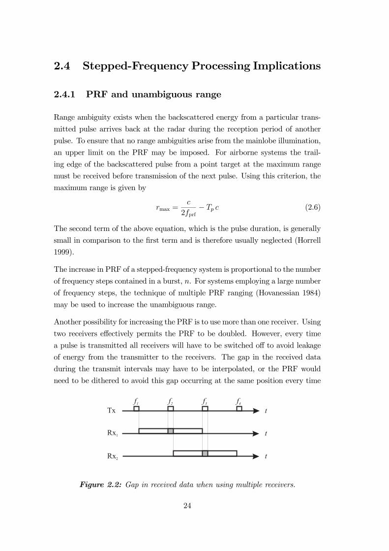
2.4 Stepped-Frequency Processing Implications
2.4.1 PRF and unambiguous range
Range ambiguity exists when the backscattered energy from a particular trans-
mitted pulse arrives back at the radar during the reception period of another
pulse. To ensure that no range ambiguities arise from the mainlobe illumination,
an upper limit on the PRF may be imposed. For airborne systems the trail-
ing edge of the backscattered pulse from a point target at the maximum range
must be received before transmission of the next pulse. Using this criterion, the
maximum range is given by
rmax =c
2fprf− Tp c (2.6)
The second term of the above equation, which is the pulse duration, is generally
small in comparison to the first term and is therefore usually neglected (Horrell
1999).
The increase in PRF of a stepped-frequency system is proportional to the number
of frequency steps contained in a burst, n. For systems employing a large number
of frequency steps, the technique of multiple PRF ranging (Hovanessian 1984)
may be used to increase the unambiguous range.
Another possibility for increasing the PRF is to use more than one receiver. Using
two receivers effectively permits the PRF to be doubled. However, every time
a pulse is transmitted all receivers will have to be switched off to avoid leakage
of energy from the transmitter to the receivers. The gap in the received data
during the transmit intervals may have to be interpolated, or the PRF would
need to be dithered to avoid this gap occurring at the same position every time
f1
Tx
Rx1
Rx2
f2 f3 f4
t
t
t
Figure 2.2: Gap in received data when using multiple receivers.
24

a pulse is transmitted. This gap in the received data is illustrated by the grey
areas in Figure 2.2.
2.4.2 Velocity compensation
The stepped-frequency signal processing methods described in this chapter all
assume that the illuminated target is stationary. If the target is moving, the
range-shift that results from the target being at a slightly different position on
a pulse-to-pulse basis can be compensated for by multiplying the spectrum of
each return by an appropriate phase ramp, according to the Fourier time-shift
theorem
f(t− ti)⇒ F (ω) e−jωti (2.7)
with
ti =2∆ric
(2.8)
and
∆ri =i vtfprf
(2.9)
where i = 0 . . . (n − 1) with n representing the number of frequency steps inone burst and vt is the radial velocity of the target, positive values representing
approaching targets. In practice, the resulting range-shift of moving targets will
be less than the width of one coarse range bin, given for example the parameters
of the L-band search radar shown in Table 2.1. It is therefore more important to
compensate for the phase shift that results from the target being at a different
location at each frequency step. The appropriate phase, that has to be added to
each return, is given by
φi =−4π∆ri fi
c(2.10)
where fi is the centre frequency of the i th frequency step.
2.4.3 Motion compensation
Motion compensation is an important topic for airborne SAR systems, and espe-
cially for ultra-wideband SAR systems. It requires that all signals are effectively
moved along a straight reference line which is defined along the aircraft flight
line. In this way, equally spaced azimuth samples along this straight reference
line can be derived for the azimuth compression operation.
25
A similar task is performed when all the sub-band signals are combined to effec-
tively form a signal which is the same as the received echo with one continuous
transmit signal under the start-stop approximation. It is important that all the
sub-band signals are combined coherently without any discontinuities at the sub-
band boundaries. If any discontinuities in phase or amplitude exist, the range
resolution may degrade and the sidelobe level may increase. Furthermore, all
sub-band signals must be collected before the aircraft moves by half the antenna
length, in order to satisfy the Nyquist sampling requirement. When combin-
ing the sub-band data, each sub-band is effectively moved to one point along
the flight line. Therefore, when the sub-band data are combined, the motion
compensation can be implemented simultaneously.
Although motion compensation has not been investigated in this thesis, it is
noteworthy to mention that the motion compensation phase shift applied to
each range line is dependent on the centre frequency of the transmitted pulse.
Referring to Equation 2.29, the baseband returned signal after demodulation is
vbb(t, i) = p (t− t0) exp (−j2πfit0) (2.11)
where the phase term exp (−j2πfit0) includes the carrier frequency fi of the i thfrequency step, and an expression for the time shift t0 = 2rt
c, determined by
the radar-target distance rt. For a stepped-frequency system this implies that
separate motion compensation must be performed on each narrowband pulse,
rather than applying motion compensation to the reconstructed wideband signal.
More information on motion compensation, particularly regarding the SASAR
system, is given by (Horrell 1999).
2.5 IFFT Method
2.5.1 Overview
To obtain a high-resolution synthetic range profile from stepped-frequency data
using the IFFT method entails the following steps (Wehner 1995):
1. Transmit a burst of n pulses, each pulse shifted in frequency by a fixed
frequency step size, ∆f .
26
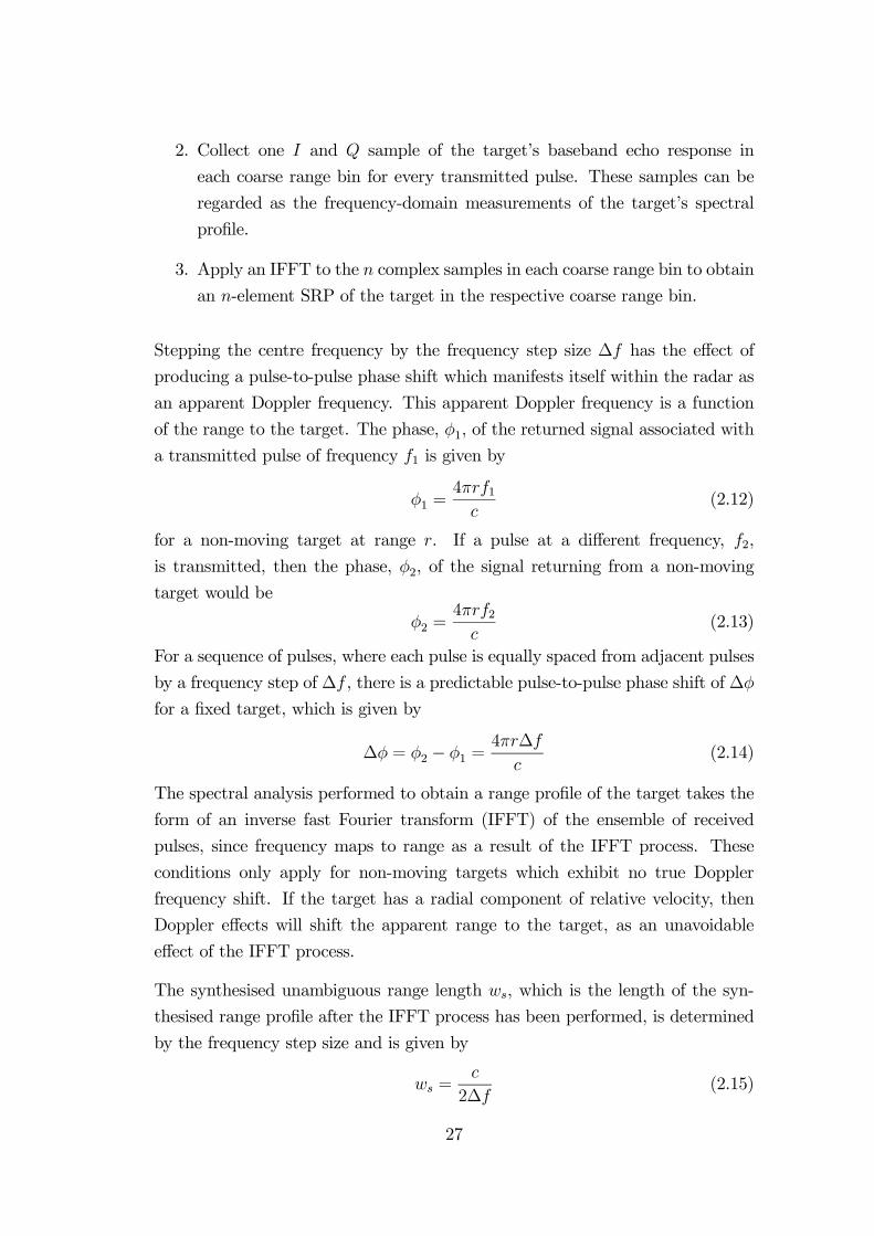
2. Collect one I and Q sample of the target’s baseband echo response in
each coarse range bin for every transmitted pulse. These samples can be
regarded as the frequency-domain measurements of the target’s spectral
profile.
3. Apply an IFFT to the n complex samples in each coarse range bin to obtain
an n-element SRP of the target in the respective coarse range bin.
Stepping the centre frequency by the frequency step size ∆f has the effect of
producing a pulse-to-pulse phase shift which manifests itself within the radar as
an apparent Doppler frequency. This apparent Doppler frequency is a function
of the range to the target. The phase, φ1, of the returned signal associated with
a transmitted pulse of frequency f1 is given by
φ1 =4πrf1c
(2.12)
for a non-moving target at range r. If a pulse at a different frequency, f2,
is transmitted, then the phase, φ2, of the signal returning from a non-moving
target would be
φ2 =4πrf2c
(2.13)
For a sequence of pulses, where each pulse is equally spaced from adjacent pulses
by a frequency step of ∆f , there is a predictable pulse-to-pulse phase shift of ∆φ
for a fixed target, which is given by
∆φ = φ2 − φ1 =4πr∆f
c(2.14)
The spectral analysis performed to obtain a range profile of the target takes the
form of an inverse fast Fourier transform (IFFT) of the ensemble of received
pulses, since frequency maps to range as a result of the IFFT process. These
conditions only apply for non-moving targets which exhibit no true Doppler
frequency shift. If the target has a radial component of relative velocity, then
Doppler effects will shift the apparent range to the target, as an unavoidable
effect of the IFFT process.
The synthesised unambiguous range length ws, which is the length of the syn-
thesised range profile after the IFFT process has been performed, is determined
by the frequency step size and is given by
ws =c
2∆f(2.15)
27
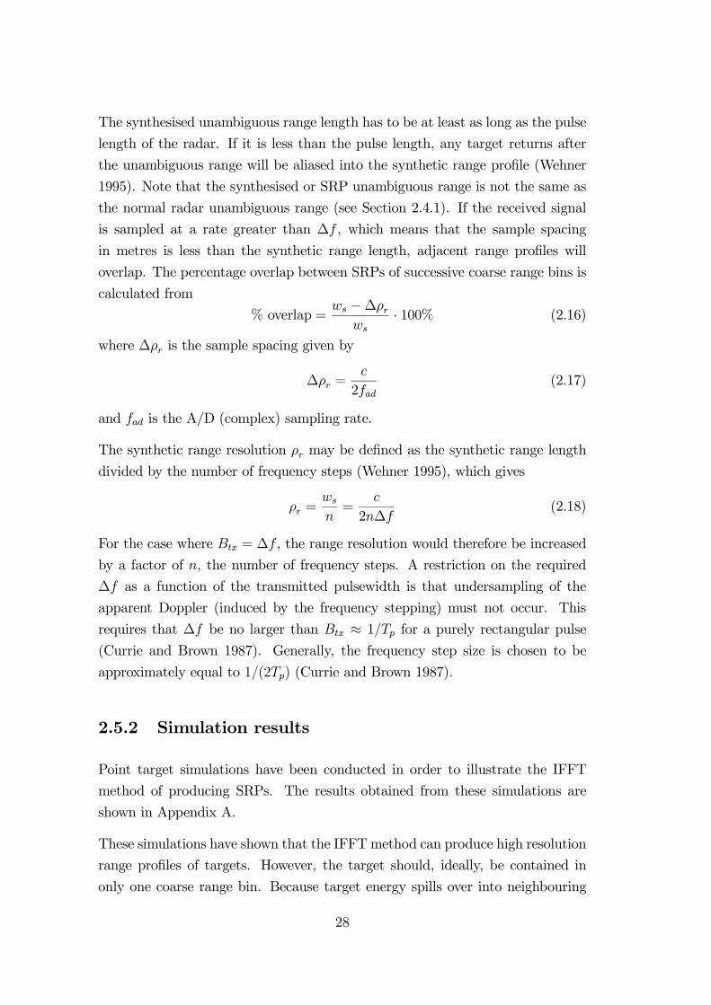
The synthesised unambiguous range length has to be at least as long as the pulse
length of the radar. If it is less than the pulse length, any target returns after
the unambiguous range will be aliased into the synthetic range profile (Wehner
1995). Note that the synthesised or SRP unambiguous range is not the same as
the normal radar unambiguous range (see Section 2.4.1). If the received signal
is sampled at a rate greater than ∆f , which means that the sample spacing
in metres is less than the synthetic range length, adjacent range profiles will
overlap. The percentage overlap between SRPs of successive coarse range bins is
calculated from
% overlap =ws −∆ρrws
· 100% (2.16)
where ∆ρr is the sample spacing given by
∆ρr =c
2fad(2.17)
and fad is the A/D (complex) sampling rate.
The synthetic range resolution ρr may be defined as the synthetic range length
divided by the number of frequency steps (Wehner 1995), which gives
ρr =wsn=
c
2n∆f(2.18)
For the case where Btx = ∆f , the range resolution would therefore be increased
by a factor of n, the number of frequency steps. A restriction on the required
∆f as a function of the transmitted pulsewidth is that undersampling of the
apparent Doppler (induced by the frequency stepping) must not occur. This
requires that ∆f be no larger than Btx ≈ 1/Tp for a purely rectangular pulse(Currie and Brown 1987). Generally, the frequency step size is chosen to be
approximately equal to 1/(2Tp) (Currie and Brown 1987).
2.5.2 Simulation results
Point target simulations have been conducted in order to illustrate the IFFT
method of producing SRPs. The results obtained from these simulations are
shown in Appendix A.
These simulations have shown that the IFFTmethod can produce high resolution
range profiles of targets. However, the target should, ideally, be contained in
only one coarse range bin. Because target energy spills over into neighbouring
28
coarse range bins, this method is not suited to the production of range profiles
of extended targets covering many coarse range bins, and is therefore also not
suited for SAR processing applications.
2.5.3 Results from stepped-frequency aircraft data
Over the last few years a substantial amount of work has been carried out at
UCT to produce SRPs of aircraft targets using an L-band search radar. The high
range resolution that can be obtained from SRP processing makes it feasible to
extract characteristic features from a profile obtained from an aircraft. The
ultimate aim of producing SRPs is to use these extracted features for non-co-
operative target recognition (NCTR), so as to be able to identify an aircraft
type from the echo signal received by the radar. The feasibility of using stepped-
frequency waveforms to produce high resolution down-range profiles has already
been demonstrated by the production of SRPs of aeroplanes (Robinson and Inggs
1994). More information regarding the NCTR project can be obtained from
(Inggs and Lord 1996) and (Lengenfelder 1998a).
Start frequency f0 1265.0MHz
Frequency step size ∆f 1.5MHz
Number of steps n 66
Chirp bandwidth Btx 3.6364MHz
ADC sample rate fad 3.75MHz
Number of coarse range bins 64
Coarse range bin length ∆ρr =c
2 fad40.0 m
Pulse length Tp 5µs
Antenna Rotation Rate θ̇ 30 rpm
Table 2.1: Parameters of L-band stepped-frequency radar system.
Table 2.1 summarises the parameters of the radar system used to obtain the
stepped-frequency aircraft database. The total radar bandwidth is given by
Bt = n∆f
= 66 · 1.5MHz = 99MHz (2.19)
which gives a synthetic range profile resolution of
ρr =c
2Bt= 1.52m (2.20)
29
This resolution is expected to be sufficient to resolve the characteristic features
of an aircraft, such as the cockpit, hull, engines, etc. The length of the synthetic
range profile is
ws =c
2∆f= 100m (2.21)
This length should be sufficient to contain even the largest aircraft. Since the re-
turned echo is sampled every c2 fad
= 40m, the synthetic range profiles associated
with the coarse range bins have an overlap of 60m.
The experience gained from producing synthetic range profiles from the stepped-
frequency aircraft data is summarised as follows:
• Decide whether or not to do moving target indication (MTI) processing.For each frequency step, two pulses were transmitted, in order to perform
MTI processing, which is implemented by subtracting the return of one
pulse from the return of the other. However, this has not always yielded
the best results, especially when the radial speed of the aircraft was low.
The SRPs shown in this thesis have been obtained by taking the average
of the two pulses.
• Remove the DC component of the data.An analysis of the data has revealed that the I and Q values of the data
contain a DC-offset. (This offset would not be as severe if MTI processing
had been applied.) If this offset is not removed, the IFFT operation pro-
duces a DC peak, which will mistakenly be regarded as an aircraft feature.
• Apply velocity compensation.It has been shown that velocity compensation is very important in order to
produce accurate range profiles. Unfortunately, the radial velocity is not
accurately known for the aircraft data. An estimate has been calculated
by interpolating the flight path described in the recorded data log file.
• Select the coarse range bin containing the target.From the 64 coarse range bins, select the one with the maximum absolute
peak value, since it is the one most likely to contain the aircraft. Instances
where this was not the case could usually be attributed to clutter return.
30

Figure 2.3: (a) Synthetic range profile of a real Boeing 737; (b) Five adjacentSRPs of the Boeing, appropriately overlapped.
• Apply an IFFT across all 66 frequency steps to obtain the SRP.A circular shift may be applied to the result in order to display the peak
in the centre of the profile.
Figure 2.3 (a) shows the synthetic range profile of a real Boeing 737, which has
been upsampled by a factor of 20. Figure 2.3 (b) shows five adjacent, overlapped
range profiles of the Boeing. A large amount of spill-over of target energy into
neighbouring range bins is evident.
31

2.5.4 SAR processing using IFFT method
In order to perform SAR processing from stepped-frequency waveforms, it is im-
portant that the process which combines the stepped-frequencies should produce
synthetic range profiles that do not contain repeated target artefacts or so-called
“ghost” targets. The IFFT method described in this chapter is a very efficient
and easy way of obtaining high-resolution range profiles of targets such as air-
craft. Although successful results have been obtained, the IFFT-based method
is not a true model for reconstructing target profiles, but rather a robust estima-
tor. Due to the matched filter effect, and because of sampling at a rate greater
than the Nyquist rate, target energy spills over into neighbouring coarse range
bins. This causes repeated replicas of the target to appear in the resulting syn-
thetic range profile. The simulation results and the results obtained from real
stepped-frequency aircraft data have shown that these “ghost” images are very
significant, and therefore the IFFT method is not a suitable method to use when
processing stepped-frequency SAR data.
The next section introduces an alternative method of producing synthetic range
profiles which does not produce these “ghost” targets and is therefore more suit-
able for stepped-frequency SAR processing applications.
2.6 Time-Domain Reconstruction of Wideband
Chirp Signal
2.6.1 Introduction
The concept of combining an ensemble of narrow-bandwidth chirp waveforms to
produce one wide-bandwidth chirp waveform is illustrated in Figure 2.4. In the
figure, two narrow-bandwidth chirp waveforms at baseband are shown. Before
combining these two waveforms coherently to form the wide-bandwidth chirp
waveform, they have to be upsampled and shifted in frequency, and a phase-
correction term has to be added to each of them.
Since the narrow-bandwidth chirp waveforms are essentially fractions of a recon-
structed wide-bandwidth chirp waveform, it is required that each of them should
have the same chirp rate γ. Furthermore, in order to avoid gaps or overlaps in
32
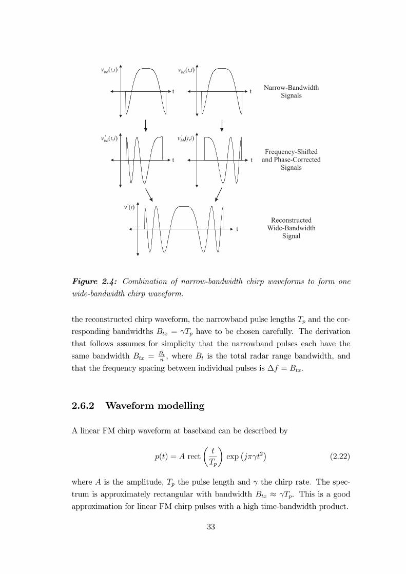
t
t t
t
tNarrow-Bandwidth
Signals
Frequency-Shiftedand Phase-Corrected
Signals
ReconstructedWide-Bandwidth
Signal
vbb( , )t i vbb( , )t i
vbb( , )t i' vbb( , )t i'
v ( )t'
Figure 2.4: Combination of narrow-bandwidth chirp waveforms to form one
wide-bandwidth chirp waveform.
the reconstructed chirp waveform, the narrowband pulse lengths Tp and the cor-
responding bandwidths Btx = γTp have to be chosen carefully. The derivation
that follows assumes for simplicity that the narrowband pulses each have the
same bandwidth Btx = Btn, where Bt is the total radar range bandwidth, and
that the frequency spacing between individual pulses is ∆f = Btx.
2.6.2 Waveform modelling
A linear FM chirp waveform at baseband can be described by
p(t) = A rectt
Tpexp jπγt2 (2.22)
where A is the amplitude, Tp the pulse length and γ the chirp rate. The spec-
trum is approximately rectangular with bandwidth Btx ≈ γTp. This is a good
approximation for linear FM chirp pulses with a high time-bandwidth product.
33
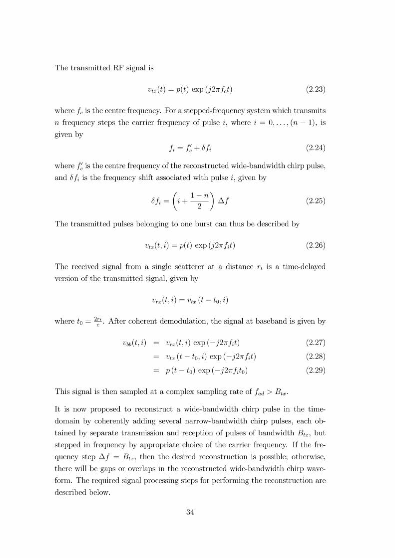
The transmitted RF signal is
vtx(t) = p(t) exp (j2πfct) (2.23)
where fc is the centre frequency. For a stepped-frequency system which transmits
n frequency steps the carrier frequency of pulse i, where i = 0, . . . , (n − 1), isgiven by
fi = fc + δfi (2.24)
where fc is the centre frequency of the reconstructed wide-bandwidth chirp pulse,
and δfi is the frequency shift associated with pulse i, given by
δfi = i+1− n2
∆f (2.25)
The transmitted pulses belonging to one burst can thus be described by
vtx(t, i) = p(t) exp (j2πfit) (2.26)
The received signal from a single scatterer at a distance rt is a time-delayed
version of the transmitted signal, given by
vrx(t, i) = vtx (t− t0, i)
where t0 = 2rtc. After coherent demodulation, the signal at baseband is given by
vbb(t, i) = vrx(t, i) exp (−j2πfit) (2.27)
= vtx (t− t0, i) exp (−j2πfit) (2.28)
= p (t− t0) exp (−j2πfit0) (2.29)
This signal is then sampled at a complex sampling rate of fad > Btx.
It is now proposed to reconstruct a wide-bandwidth chirp pulse in the time-
domain by coherently adding several narrow-bandwidth chirp pulses, each ob-
tained by separate transmission and reception of pulses of bandwidth Btx, but
stepped in frequency by appropriate choice of the carrier frequency. If the fre-
quency step ∆f = Btx, then the desired reconstruction is possible; otherwise,
there will be gaps or overlaps in the reconstructed wide-bandwidth chirp wave-
form. The required signal processing steps for performing the reconstruction are
described below.
34
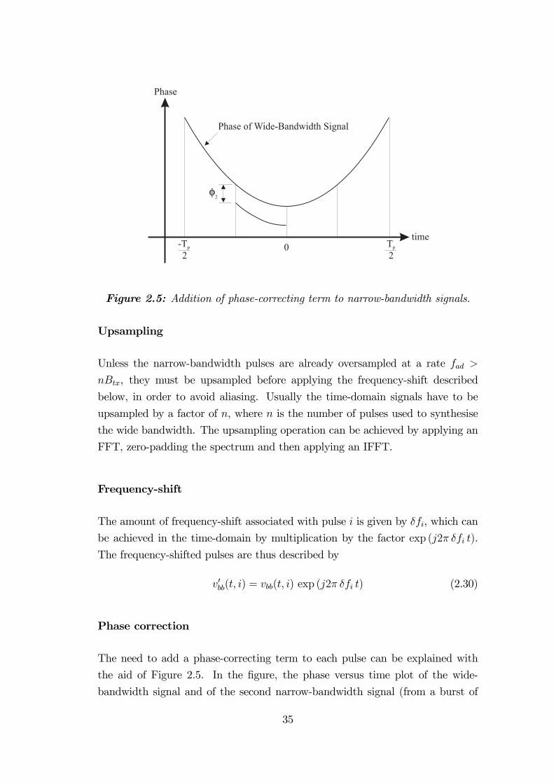
Tp
2
2
time
Phase
Phase of Wide-Bandwidth Signal
-Tp
20
Figure 2.5: Addition of phase-correcting term to narrow-bandwidth signals.
Upsampling
Unless the narrow-bandwidth pulses are already oversampled at a rate fad >
nBtx, they must be upsampled before applying the frequency-shift described
below, in order to avoid aliasing. Usually the time-domain signals have to be
upsampled by a factor of n, where n is the number of pulses used to synthesise
the wide bandwidth. The upsampling operation can be achieved by applying an
FFT, zero-padding the spectrum and then applying an IFFT.
Frequency-shift
The amount of frequency-shift associated with pulse i is given by δfi, which can
be achieved in the time-domain by multiplication by the factor exp (j2π δfi t).
The frequency-shifted pulses are thus described by
vbb(t, i) = vbb(t, i) exp (j2π δfi t) (2.30)
Phase correction
The need to add a phase-correcting term to each pulse can be explained with
the aid of Figure 2.5. In the figure, the phase versus time plot of the wide-
bandwidth signal and of the second narrow-bandwidth signal (from a burst of
35

four such signals) is shown. The narrow-bandwidth signal has already been
shifted in frequency and time, but a phase-correcting term given by
φi = exp jπγT 2p i+1− n2
2
(2.31)
has to be applied in order to avoid phase discontinuities in the wide-bandwidth
signal. This phase term may be applied to the narrow-bandwidth signals before
they are upsampled, thus requiring fewer multiplications and leading to a faster
implementation of the procedure.
Time-shift
Before adding the narrow-bandwidth pulses together, they have to be shifted in
the time domain. The necessary time-shift is given by
δti = i+1− n2
Tp (2.32)
Since the signals are sampled at the A/D rate fad (after they have been upsam-
pled), the time-shift given in terms of number of samples is
mi = δti fad (2.33)
Ideally mi should be an integer, because fractional values would require the
narrow-bandwidth pulses to be interpolated. This would be computationally
inefficient and might lead to errors in the reconstructed wide-bandwidth signal.
This requirement can be achieved by adjusting either the pulse length Tp or the
A/D sampling rate fad.
2.6.3 Combining narrow-bandwidth chirps
The reconstructed wide-bandwidth signal v (t) is obtained by coherently adding
the processed narrow-bandwidth signals. Observing that ∆f = Btx = γTp, one
obtains the following expression for v (t) after simplification:
v (t) =n−1
i=0
vbb(t− δti, i)φi (2.34)
=n−1
i=0
A rectt− 2rt
c− δti
Tpexp jπγ t− 2rt
c− δti
2
36
· exp j2πfi t− 2rtc− δti exp [−j2πfi (t− δti)]
· exp [j2π δfi (t− δti)] exp jπγT 2p i+1− n2
2
(2.35)
= A exp jπγ t− 2rtc
2 n−1
i=0
rectt− 2rt
c− δti
Tp(2.36)
= A exp jπγ t− 2rtc
2
rectt− 2rt
c
nTp(2.37)
This is simply the expression of a wide-bandwidth chirp pulse with a bandwidth
of Bt ≈ γTp = nBtx, with Tp = nTp. Range compression may be achieved by
convolving this signal with a matched filter, which is given by the time-reversed
conjugate of the wide-bandwidth pulse.
2.6.4 Simulation results
A stepped-frequency radar system was simulated to validate and illustrate the
method described above. Table 2.2 summarises the relevant parameters used.
These parameters were chosen to correspond with the VHF-band SASAR system,
which has a centre frequency fc = 141MHz and transmits linear FM chirps with
a pulse length of Tp = 10µs (among others) and a bandwidth of Btx = 12MHz
sampled at fad = 24MHz. In the simulation, four pulses were transmitted, each
with a bandwidth of 12MHz, spaced at 12MHz intervals. The total radar band-
width is given by Bt = nBtx = 48MHz, and therefore the expected resolution
is 2.78m, which includes the mainlobe broadening factor Kr = 0.89 associated
with a rectangular weighting window. (Note that the current SASAR system
cannot achieve such a bandwidth due to antenna and receiver limitations.)
First centre frequency f0 123MHz
Frequency step size ∆f 12MHz
Number of steps n 4
Bandwidth of narrowband chirp pulses Btx 12MHz
ADC (complex) sample rate fad 24MHz
Pulse length of narrowband chirp pulses Tp 10µs
Total radar bandwidth Bt 48MHz
Table 2.2: Stepped-frequency simulation parameters of time-domain method.
37

Figure 2.6: Simulation results of time-domain method to combine stepped-
frequency waveforms.
The results of the simulation are summarised in Figure 2.6, which displays the
following graphs:
(a) The real return of the first narrowband chirp pulse.
(b) The real part of the reconstructed wideband chirp waveform, which has a
bandwidth of Bt = 48MHz.
(c) A dB plot of the entire range profile, after the signal shown in (b) has been
range compressed.
(d) A zoomed-in portion of the range profile, after the complex data has been
upsampled by a factor of 100.
The peak sidelobe levels have been measured to be −13.2dB below the main-lobe, which agrees with the expected theoretical value when using a rectangular
38

window function. The integrated sidelobe ratio, measured across the range ex-
tent shown in Figure 2.6 (d), was calculated to be −10.6dB, and the measured3dB mainlobe width was 2.79m, which also agrees with the expected value.
This simulation illustrates that the time-domain method can be used to combine
stepped-frequency waveforms without introducing repeated target artefacts in
the high-resolution range profile.
2.6.5 Results using E-SAR data
In order to verify the stepped-frequency time-domain approach on real data, the
range frequency spectrum of a raw German E-SAR C-band image of Lechfeld,
Germany, was divided into five parts, each part approximating the frequency
spectrum of a fictitious narrow-bandwidth pulse. It is only an approximation,
since the rectangular window, which was used to split the wide-bandwidth fre-
quency spectrum, introduces ringing in the time domain. Nevertheless, an inverse
FFT was then applied to the narrow-bandwidth spectra, effectively yielding the
time-domain return of five narrow-bandwidth pulses. Table 2.3 shows the rele-
vant parameters of the original E-SAR image. After dividing the range spectrum
into five parts, the centre frequency of the first pulse became f0 = 5.26GHz, the
bandwidth of each narrowband pulse became Btx = 20MHz, the sampling rate
was reduced to 20MHz and the pulse lengths were reduced to 1µs.
Figure 2.7 shows the result which was obtained after processing the image with
the chirp scaling algorithm using only one of the five frequency steps. After com-
bining all five frequency steps using the time-domain method, the image shown
in Figure 2.8 was obtained. The improvement in range resolution is clearly visi-
ble. No visible difference could be detected between this image and the original
wideband image, except for the fact that targets at near and far range became
fainter. This is the result of information having been shifted out of the range ex-
tent when the time-shift was performed. According to Equation 2.33, 200 range
Centre frequency fc 5.3GHz
Total radar bandwidth Bt 100MHz
A/D (complex) sample rate fad 100MHz
Pulse length Tp 5µs
Table 2.3: Parameters of E-SAR image.
39
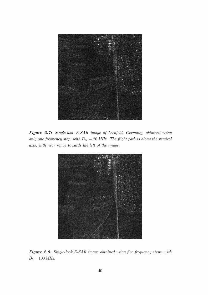
Figure 2.7: Single-look E-SAR image of Lechfeld, Germany, obtained using
only one frequency step, with Btx = 20MHz. The flight path is along the vertical
axis, with near range towards the left of the image.
Figure 2.8: Single-look E-SAR image obtained using five frequency steps, withBt = 100MHz.
40

bins were shifted out of the range extent at both ends of the swath, which is a
significant number for this image, which is only 760 range bins wide.
2.6.6 SAR processing using time-domain method
The time-domain method of combining stepped-frequency waveforms has a few
disadvantages, one of them being that information is shifted out of the range
extent as in the example described above. Furthermore, in order to reconstruct
the wide-bandwidth chirp signal perfectly, the spectra of the individual frequency
steps may not overlap or contain gaps. Most importantly, however, this method
is inefficient because of the upsampling requirement described in Section 2.6.2,
and is therefore not suited for SAR processing applications. These considera-
tions have led to the development of a frequency-domain method described in
Chapter 3, which does not have these drawbacks.
2.7 Review and Summary
This chapter has given a brief introduction to side-looking strip-map SAR. The
concept of range resolution has been described, and there has been discussion of
how it applies to short pulse systems, pulse compression systems and stepped-
frequency systems. The implications of a stepped-frequency system, such as the
increase in PRF, velocity compensation and motion compensation have been
discussed.
The IFFT method of processing stepped-frequency data has been applied on
simulated data and on real stepped-frequency data of aircraft. Experience gained
from applying the IFFT method has shown it to be unsuitable for processing
SAR images, mainly because target energy spills over into consecutive coarse
range bins as a result of the matched filter operation, causing “ghost targets”
in the range profile. The time-domain approach is also not suitable for SAR
applications, mainly because it is very inefficient to upsample the narrowband
pulses in the time-domain.
Instead of recombining the stepped-frequency waveforms in the time-domain,
they can also be recombined in the frequency domain. Essentially the aim is to
reconstruct a larger portion of the target’s reflectivity spectrum Z(f) by com-
41

bining the individual spectra of the transmitted narrow-bandwidth pulses in the
frequency domain. The target reflectivity function ζ(t) represents the target’s
reflection properties at range r mapped into the time domain, where t = 2rc. This
method is described in Chapter 3. It will be shown that the frequency-domain
approach efficiently uses all of the information contained in the stepped-frequency
data to produce reliable, high-resolution range profiles, which do not contain any
repeating artefacts or “ghost targets”.
The IFFT method can be seen to be a limiting case of the spectrum reconstruc-
tion method. Instead of obtaining the narrowband spectrum for every transmit-
ted pulse and then shifting and coherently adding all the subspectra to recon-
struct the target’s reflectivity spectrum, the IFFT method only operates on the
coarse range bin containing the largest magnitude return. This value is regarded
as a sample of the target’s reflectivity spectrum. Both methods apply an inverse
FFT to their respective target reflectivity spectrum to obtain a high-resolution
time-domain range profile. The IFFT method only works well for targets which
are completely contained in one coarse range bin, but it is unsuitable for extended
targets or SAR applications.
The time-domain technique is also similar to the frequency-domain technique.
Both methods require the narrowband pulses to be shifted in frequency, after
which they are coherently added. However, the time-domain pulses need to be
upsampled before applying the frequency shift, making this method computa-
tionally intensive and inefficient.
42

Chapter 3
Reconstruction of TargetReflectivity Spectrum
3.1 Introduction
The concept of reconstructing a target’s reflectivity spectrum by coherently
adding all the narrowband spectra in the frequency domain has already been
introduced in the previous chapter. This chapter describes this approach of
processing stepped-frequency data in more detail. Section 3.2 gives the mathe-
matical background, and Sections 3.3 and 3.4 describe the steps involved when
reconstructing the target’s reflectivity spectrum. Section 3.5 describes the design
of the compression filter, which flattens the spectral “ripples” at the subspec-
tra boundaries, that would otherwise produce repeating artefacts in the time-
domain.
This technique involves the reconstruction of a wider portion of the target’s
reflectivity spectrum by combining the individual spectra of the transmitted
narrow-bandwidth pulses in the frequency domain. The principle of enhancing
the range resolution by recovering a larger band of the reflectivity’s spectrum
was introduced by Prati and Rocca (Prati and Rocca 1992), but that was in the
context of coherently combining SAR images taken from different observation
angles. This thesis shows how the technique may be applied to the concept of
stepped-frequency processing.
The CARABAS-II system, which operates in the 20—90MHz band, also em-
43

ploys stepped-frequency processing to obtain a bandwidth of 70MHz (Ulander
1998), (Ulander and Frölind 1999). The CARABAS-II processing method has
been independently developed but is very similar to the method described in
this chapter, since it also involves the coherent addition of complex narrowband
subspectra to reconstruct the wide-bandwidth spectrum. To the best of the
candidate’s knowledge, the concept of describing this technique in terms of the
target reflectivity profile is novel.
The technique is verified and illustrated in Section 3.6 by implementing it on
simulated data. It is shown how frequencies may be skipped in order to avoid
spectral regions that would be corrupted by RFI. It is also shown that both
the frequency step sizes and the individual transmit bandwidths within a burst
of pulses can be varied. This offers more flexibility in notching out specific
regions of the spectrum that contain dominant interferers. Section 3.7 describes
the results that have been obtained when applying this technique on the real
stepped-frequency aircraft data described in the previous chapter.
The methods described in this chapter adopt the start-stop approximation, which
means that the radar-target range remains constant during the transmission of
one burst of frequencies. The candidate is indebted to AndrewWilkinson (RRSG,
UCT) for the mathematical modelling and description of this technique (Wilkin-
son 1996), reviewed in Sections 3.2—3.5. Only the coding, implementation and
characterization of the performance of this method are the candidate’s own work.
Some of the material in this chapter has been published in the Proceedings of
COMSIG’98 (Wilkinson, Lord and Inggs 1998).
3.2 Waveform Modelling
For reasons of flow and ease of reading, the first few equations of Section 2.6.2
are repeated here. Thus, as already mentioned, a linear FM chirp waveform at
baseband can be described by
p(t) = A rectt
Tpejπγt
2
(3.1)
where A is the amplitude, Tp the pulse length and γ the chirp rate. The spec-
trum is approximately rectangular with bandwidth Btx ≈ γTp. This is a good
approximation for linear FM chirp pulses with a high time-bandwidth product.
44

The transmitted RF signal is modelled by
vtx(t) = p(t) ej2πfct (3.2)
where fc is the centre frequency. The received signal is given by the convolution
of the scene reflectivity function ζ(t) and the transmitted pulse:
vrx(t) = ζ(t) vtx(t) (3.3)
= ζ(t− τ) vtx(τ) dτ (3.4)
After coherent demodulation, the signal at baseband is given by
vbb(t) = vrx(t) e−j2πfct (3.5)
= ζ(t− τ) p(τ) ej2πfcτ dτ e−j2πfct (3.6)
= ζ(t− τ) e−j2πfc(t−τ) p(τ) dτ (3.7)
= ζ(t) e−j2πfct p(t) (3.8)
All linear receiver distortions (for example front-end filters, antenna responses,
etc.) can be included in the signal model by introducing an equivalent baseband
filter x(t). Receiver noise is modelled by an equivalent referred RF noise signal
n(t) with spectrum N(f). The signal as it appears at the input to the receiver
analogue to digital converter is therefore
vbb(t) = ζ(t) e−j2πfct + n(t)e−j2πfct p(t) x(t) (3.9)
This signal is sampled at a complex sampling rate of fad > Btx. In the frequency
domain the expression for the baseband signal is
Vbb(f) = [Z (f + fc) +N (f + fc)] P (f)X(f) (3.10)
Thus, the spectral representation of the received signal can be viewed as a win-
dowed version of the target’s reflectivity spectrum Z (f), where the position of
the window is determined by the centre frequency, and the shape is determined
by the spectrum of the transmitted pulse and the receiver distortions.
Range compression is usually achieved by convolving the received signal with a
matched filter, which is given by the time-reversed conjugate of the transmitted
pulse, and which maximises the instantaneous signal to noise ratio. More gener-
ally, a compression filterH(f) can be designed as a trade-off between compressing
45
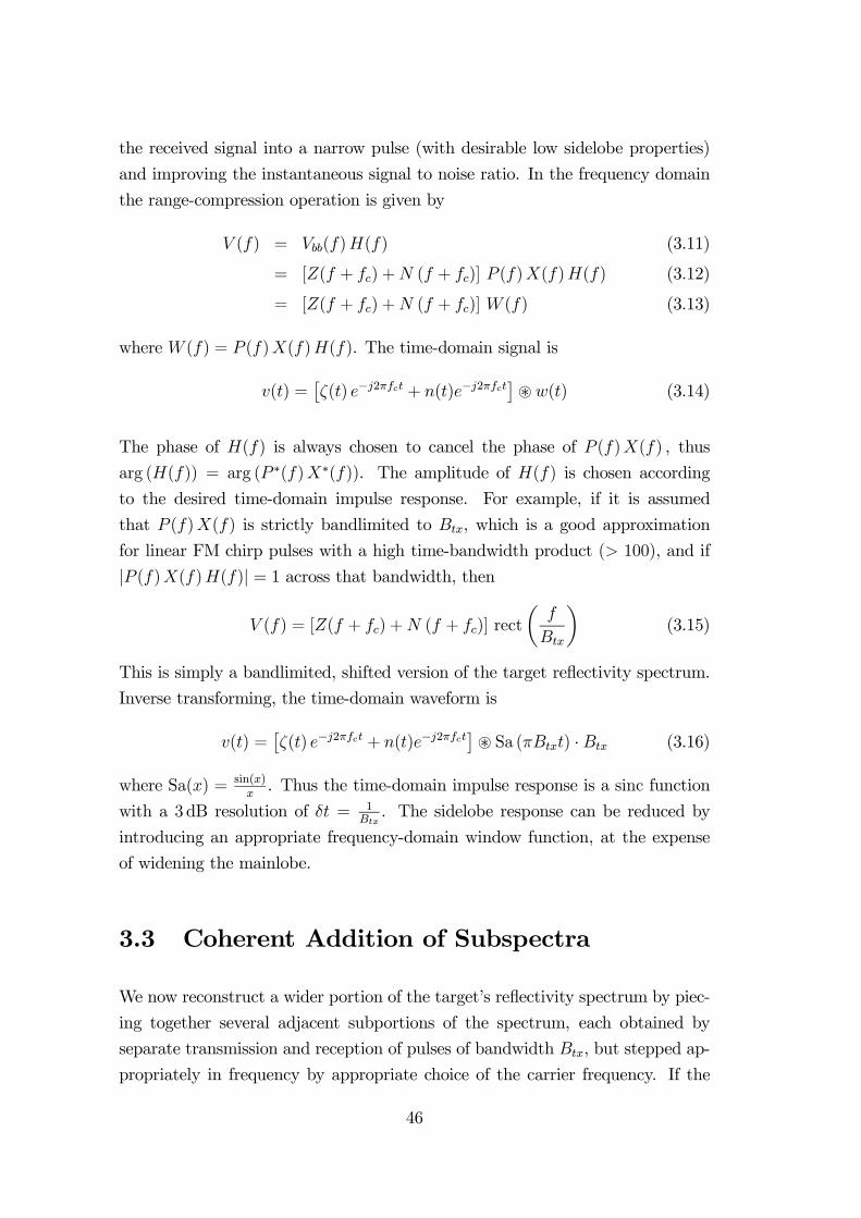
the received signal into a narrow pulse (with desirable low sidelobe properties)
and improving the instantaneous signal to noise ratio. In the frequency domain
the range-compression operation is given by
V (f) = Vbb(f)H(f) (3.11)
= [Z(f + fc) +N (f + fc)] P (f)X(f)H(f) (3.12)
= [Z(f + fc) +N (f + fc)] W (f) (3.13)
where W (f) = P (f)X(f)H(f). The time-domain signal is
v(t) = ζ(t) e−j2πfct + n(t)e−j2πfct w(t) (3.14)
The phase of H(f) is always chosen to cancel the phase of P (f)X(f) , thus
arg (H(f)) = arg (P ∗(f)X∗(f)). The amplitude of H(f) is chosen according
to the desired time-domain impulse response. For example, if it is assumed
that P (f)X(f) is strictly bandlimited to Btx, which is a good approximation
for linear FM chirp pulses with a high time-bandwidth product (> 100), and if
|P (f)X(f)H(f)| = 1 across that bandwidth, then
V (f) = [Z(f + fc) +N (f + fc)] rectf
Btx(3.15)
This is simply a bandlimited, shifted version of the target reflectivity spectrum.
Inverse transforming, the time-domain waveform is
v(t) = ζ(t) e−j2πfct + n(t)e−j2πfct Sa (πBtxt) ·Btx (3.16)
where Sa(x) = sin(x)x. Thus the time-domain impulse response is a sinc function
with a 3dB resolution of δt = 1Btx. The sidelobe response can be reduced by
introducing an appropriate frequency-domain window function, at the expense
of widening the mainlobe.
3.3 Coherent Addition of Subspectra
We now reconstruct a wider portion of the target’s reflectivity spectrum by piec-
ing together several adjacent subportions of the spectrum, each obtained by
separate transmission and reception of pulses of bandwidth Btx, but stepped ap-
propriately in frequency by appropriate choice of the carrier frequency. If the
46

frequency step ∆f satisfies the inequality ∆f ≤ Btx, then the desired recon-
struction is possible. Assuming a sequence of n adjacent windows (indexed by
i = 0, . . . , n−1), a broad region of the frequency spectrum can be reconstructed,symmetrical about zero, by shifting each spectrum at baseband by an amount
δfi = i+1− n2
∆f (3.17)
in the positive direction, and adding together the shifted versions. For an array
with M discrete bins sampled at a complex rate of fad, the frequency shift in
terms of number of samples is
mi =M
fadδfi (3.18)
Ideallymi should be an integer, because fractional values would otherwise require
the subspectra to be interpolated. This would be computationally inefficient and
might lead to errors in the reconstructed spectrum.
If we assume a linear superposition of the shifted subspectra, the reconstructed
spectrum as shown in Figure 3.1 is
V (f) =n−1
i=0
Vi(f − δfi) (3.19)
=n−1
i=0
([Z(f + fi − δfi) +N(f + fi − δfi)] W (f − δfi)) (3.20)
where fi is the carrier frequency of pulse i and Vi(f) is the frequency spec-
trum at baseband of pulse i. The expression (fi − δfi) can, by substitution and
simplification, be seen to be the centre frequency fc of the entire reconstructed
spectrum:
fc = fi − δfi (3.21)
= (f0 + i∆f)− i+1− n2
∆f (3.22)
= f0 +n− 12
∆f (3.23)
=f0 + fn−1
2(3.24)
The reconstructed spectrum can thus be expressed as
V (f) = [Z(f + fc) +N(f + fc)]n−1
i=0
W (f − δfi) (3.25)
= [Z(f + fc) +N(f + fc)] W (f) (3.26)
47

����
�����
Target Reflectivity Function
Reconstructed Target Reflectivity Spectrum
�
�
�
���Target Reflectivity Spectrum
� �� ��� ��
�
�
��
���
Baseband Spectrum
���
�
)(' fV
)(0
fV
Figure 3.1: Reconstruction of target reflectivity spectrum for n = 4 transmittedpulses, each with carrier frequency fi and bandwidth Btx.
where
W (f) =n−1
i=0
W (f − δfi) (3.27)
The time-domain signal can then be obtained by inverse transforming to yield
v (t) = ζ(t) e−j2πfct + n(t)e−j2πfct w (t) (3.28)
If, for example, we consider the case where the frequency step ∆f = Btx, then
the total bandwidth of the reconstructed spectrum is Bt = nBtx, as is shown in
Figure 3.1. If the combined compression filter
H (f) =n−1
i=0
H(f − δfi) (3.29)
is chosen such that W (f) = rect fBt, then the time-domain signal is
v (t) = ζ(t) e−j2πfct + n(t)e−j2πfct Sa(πBtt) ·Bt (3.30)
and the 3dB resolution is δt = 1Bt, which is a factor of n better than would have
been achieved without reconstruction.
48
3.4 Practical Implementation on Sampled Data
The steps below describe how the spectral reconstruction can be performed with
sampled data.
1. Choose a range of carrier frequencies f0, . . . , fn−1 spaced at ∆f equal to,
or marginally less than Btx. If ∆f > Btx, the reconstructed spectrum
will contain gaps and the resulting time-domain range profile will possess
undesirable properties in the form of repeated artifacts spaced at multi-
ples of 1∆f. However, even if there are gaps, an improvement in mainlobe
resolution is still possible.
2. For each pulse obtain a sampled version of vbb(t), starting at t0, with a
complex sampling rate fs, where fs > Btx.
3. Apply an FFT to each sampled pulse to obtain the individual subspectra
of the target’s reflectivity spectrum.
4. To obtain an optimal SNR, each subspectrum is matched-filtered prior to
addition.
5. Since vbb(t) was sampled starting at t0, each subspectrum has to be multi-
plied by the delay compensation factor exp(+j2πft0).
6. Shift the spectrum of pulse i to its appropriate location, centred on
f = i+ 1−n2
∆f .
7. Form the combined spectrum by coherently adding all of the individual
subspectra.
8. Multiply the combined spectrum by the compression filter H (f) to obtain
the discrete equivalent of V (f).
9. Multiply the entire spectrum by exp(−j2πft0). This re-shifts the timedomain back to a sampled set beginning at t = t0.
10. Apply a reshaping window, such as a Hanning or Taylor window, to sup-
press time-domain sidelobes at the expense of widening the mainlobe.
11. Inverse FFT the entire spectrum to obtain the high-resolution range profile.
49
3.5 Design of Compression Filter
The design of the compression filterH (f) is the most critical and important step
in this method. It is important to consider the following points when constructing
this filter:
• Obtain an estimate of the combined impulse response spectrum
U (f) = P (f)X (f) (3.31)
=n−1
i=0
P (f − δfi)X(f − δfi) (3.32)
For a real system, this should be achieved by measuring the return of a real,
physical point target, for example a corner reflector, and recombining the
individual spectra as described in the previous section. For such a target
Z(f) ≈ α, where α is a constant, and therefore the combined baseband
spectrum would be Vbb(f) ≈ αP (f)X (f). This method automatically
provides an accurate description of the receiver distortions given by X (f).
• If it is impractical to obtain the return of a real, physical point target,a point target simulation may be used. It may be difficult, however, to
predict the receiver distortions given by X (f). In the simulations that
follow it has been assumed that X (f) = 1. Note also that the position of
the high-resolution profile will be relative to the target range chosen in the
simulation and may therefore need to be shifted.
• If the sampled data has already been range-compressed by a matched filterto optimise the SNR, the subspectra used in constructing H (f) must also
be range-compressed first with the same matched filter.
• When using a simulation it is important to ensure that there is no aliasingand that the individual subspectra are bandlimited. In the simulations
that follow, this has been accomplished as follows:
— First the return was oversampled by an arbitrary factor of 10 in or-der to reduce aliasing. If the time-bandwidth product is relatively
high, the spectrum decays fairly quickly and a factor of 10 should be
sufficient.
50

— After applying an FFT, the corresponding spectrum was multiplied
by rect fBtx
to bandlimit the return to Btx.
— To accomplish downsampling by a factor of 10, an appropriate numberof zeroes was removed from the centre of the spectrum (i.e. the most
positive and most negative frequency components).
— An IFFT transforms the now anti-aliased and bandlimited signal backinto the time-domain.
• Having obtained an approximation of U (f), the filter H (f) is piecewise
defined as follows (refer to Figure 3.2):
H (f) =
U ∗(f)|U (fa)| for f ≤ fa
1U (f)
for fa < f < fb
U ∗(f)|U (fb)| for f ≥ fb
(3.33)
where the region [fa, fb] includes the major part of the reconstructed spec-
trum, containing all the subspectra boundaries. This will effectively smoothen
any ripples at the subspectra boundaries, yielding the desired time-domain
impulse response. The first section and the last section of H (f), where
the target spectrum decays to zero, is equated to the conjugate of U (f).
This prevents the amplification of noise for a real system, while still can-
celling the phase correctly. Note that U (f) has to be scaled appropriately
faf bf
)(' fU
Figure 3.2: Construction of compression filter H (f).
51
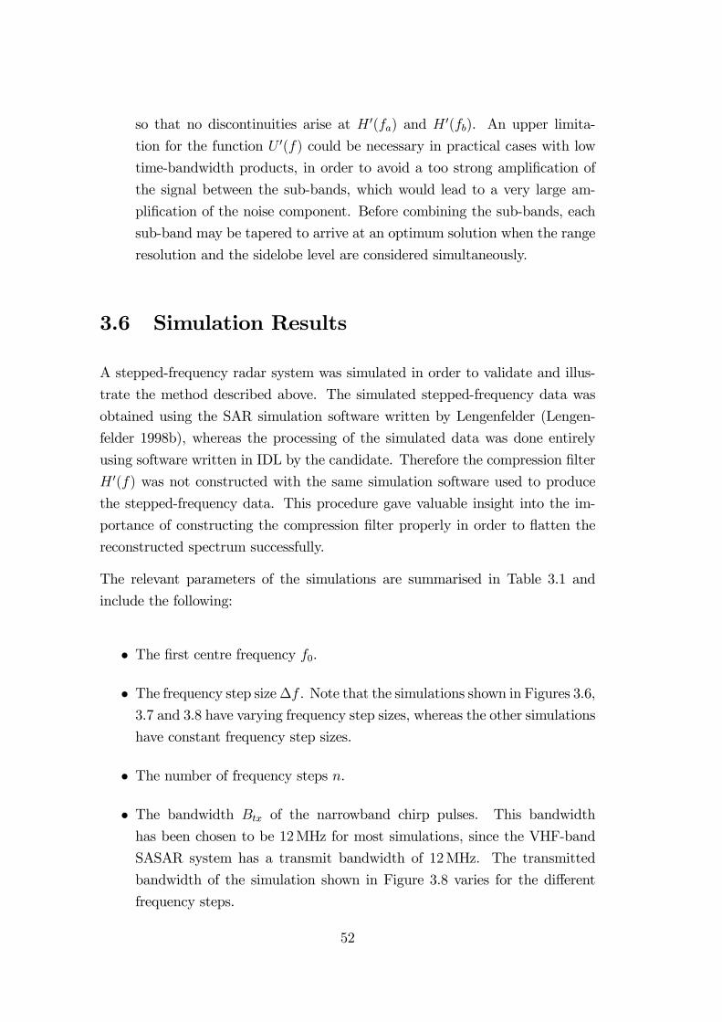
so that no discontinuities arise at H (fa) and H (fb). An upper limita-
tion for the function U (f) could be necessary in practical cases with low
time-bandwidth products, in order to avoid a too strong amplification of
the signal between the sub-bands, which would lead to a very large am-
plification of the noise component. Before combining the sub-bands, each
sub-band may be tapered to arrive at an optimum solution when the range
resolution and the sidelobe level are considered simultaneously.
3.6 Simulation Results
A stepped-frequency radar system was simulated in order to validate and illus-
trate the method described above. The simulated stepped-frequency data was
obtained using the SAR simulation software written by Lengenfelder (Lengen-
felder 1998b), whereas the processing of the simulated data was done entirely
using software written in IDL by the candidate. Therefore the compression filter
H (f) was not constructed with the same simulation software used to produce
the stepped-frequency data. This procedure gave valuable insight into the im-
portance of constructing the compression filter properly in order to flatten the
reconstructed spectrum successfully.
The relevant parameters of the simulations are summarised in Table 3.1 and
include the following:
• The first centre frequency f0.
• The frequency step size∆f . Note that the simulations shown in Figures 3.6,3.7 and 3.8 have varying frequency step sizes, whereas the other simulations
have constant frequency step sizes.
• The number of frequency steps n.
• The bandwidth Btx of the narrowband chirp pulses. This bandwidth
has been chosen to be 12MHz for most simulations, since the VHF-band
SASAR system has a transmit bandwidth of 12MHz. The transmitted
bandwidth of the simulation shown in Figure 3.8 varies for the different
frequency steps.
52

Fig. f0 ∆f n Btx fc Bt Overlap
[MHz] [MHz] [MHz] [MHz] [MHz] [MHz]
3.3 123 12 4 12 141 48 0
3.4 124.8 10.8 4 12 141 44.4 1.2
3.5 119.4 14.4 4 12 141 55.2 −2.43.6 124.8 21.6, 10.8 3 12 141 44.4 −9.6, 1.23.7 123 9, 12.9, 14.1 4 12 141 48 3, −0.9, −2.13.8 123 9, 15, 15 4 12, 8, 14, 6 141 48 1, −4, −53.9 1363.75 1.875 55 3.636 1314 104.9 1.761
3.10 1363.75 1.875 55 3.636 1314 104.9 1.761
Table 3.1: Stepped-frequency simulation parameters of spectrum reconstruction
method.
• The centre frequency fc of the entire reconstructed spectrum, which is themidpoint between the two outer edges of the reconstructed spectrum. The
centre frequency has been chosen to be 141MHz for most simulations, since
this is the centre frequency of the SASAR system.
• The total bandwidth Bt of the reconstructed spectrum. It is calculated asthe frequency range between the two outer edges of the entire reconstructed
spectrum, regardless of any gaps that may occur in the reconstructed spec-
trum.
• The amount of spectral overlap between adjacent subspectra. Spectral gapsbetween adjacent subspectra are indicated with negative numbers. The
overlap (or gap) between adjacent subspectra varies for the simulations
shown in Figures 3.6, 3.7 and 3.8.
The simulation results are shown in Figures 3.3—3.8 on the following pages. Each
figure displays the following graphs:
(a) The magnitude of the range-compressed target return, first frequency step.
Where the target return has not been range-compressed (Figure 3.3 and
Figure 3.4), the real part of the target return is shown.
(b) The spectrum obtained after coherent addition of the frequency-shifted
subspectra.
53

(c) The spectrum of the compression filter H (f).
(d) The target reflectivity spectrum V (f) after applying the compression filter
shown in (c).
(e) A dB plot of the high-resolution range profile, after inverse Fourier trans-
forming the spectrum shown in (d). No window functions have been applied
prior to inverse Fourier transforming.
(f) A zoomed-in section of the high-resolution range profile, in order to display
the peak sidelobe level. For improved accuracy, the complex values were
interpolated (using a Shannon interpolator) to one fiftieth of a sample
to increase the accuracy when measuring the resolution (3dB mainlobe
width), peak sidelobe ratios (PSLR) and integrated sidelobe ratios (ISLR),
with the integration having been performed over the range extent shown
in this graph. The extent of the main peak region was found by defining
the main peak as the region bounded by the points at which the gradient
of the peak changed sign. The ISLR is defined here as the ratio of the
integrated energy in the sidelobe region to the integrated energy contained
in the main peak region. These results are summarised in Table 3.2.
Figure 3.3 shows a simulation where the target return signal has not been band-
limited, which is evident from the abrupt edges of the uncompressed chirp signal
shown in graph (a). This implies that the spectrum of this signal does not
decay to zero and is therefore aliased. However, the compression filter H (f)
shown in graph (c) has been constructed with bandlimited signals and is therefore
not properly matched to the reconstructed spectrum shown in graph (b). As a
result, the target reflectivity spectrum shown in graph (d) contains ripples at
the subspectra boundaries, even though there was no overlap between adjacent
subspectra. These ripples increase the sidelobes and the integrated sidelobe ratio
of the time-domain range profile (refer to Table 3.2). Graph (e) shows a dB plot
of the entire high-resolution range profile, after inverse Fourier transforming the
spectrum shown in graph (d), and graph (f) shows a zoomed-in section of this
high-resolution range profile.
54
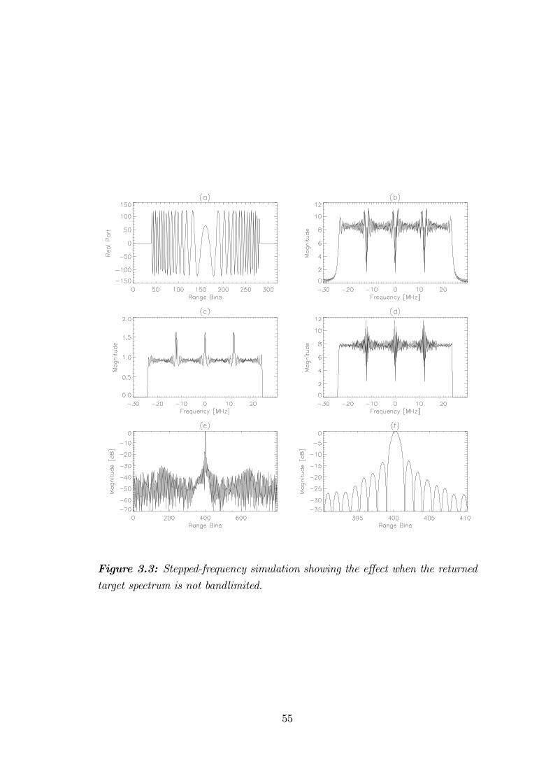
Figure 3.3: Stepped-frequency simulation showing the effect when the returnedtarget spectrum is not bandlimited.
55
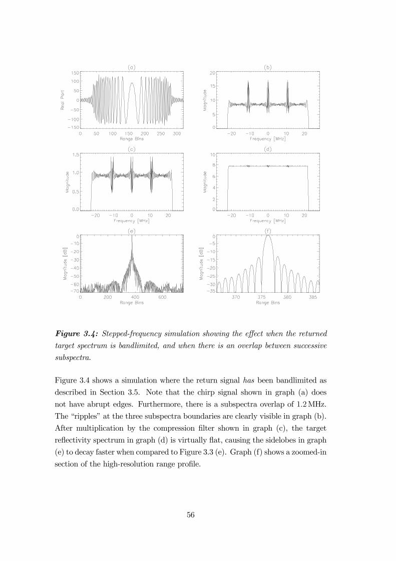
Figure 3.4: Stepped-frequency simulation showing the effect when the returnedtarget spectrum is bandlimited, and when there is an overlap between successive
subspectra.
Figure 3.4 shows a simulation where the return signal has been bandlimited as
described in Section 3.5. Note that the chirp signal shown in graph (a) does
not have abrupt edges. Furthermore, there is a subspectra overlap of 1.2MHz.
The “ripples” at the three subspectra boundaries are clearly visible in graph (b).
After multiplication by the compression filter shown in graph (c), the target
reflectivity spectrum in graph (d) is virtually flat, causing the sidelobes in graph
(e) to decay faster when compared to Figure 3.3 (e). Graph (f) shows a zoomed-in
section of the high-resolution range profile.
56
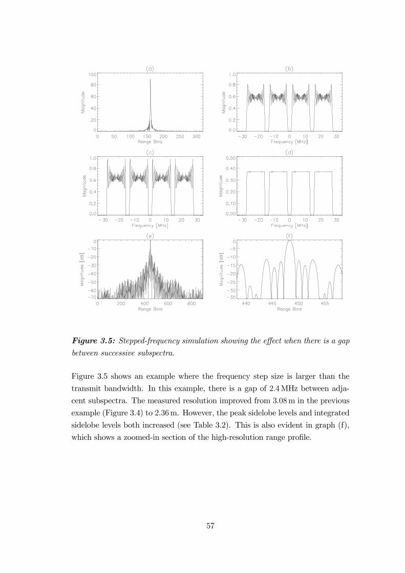
Figure 3.5: Stepped-frequency simulation showing the effect when there is a gapbetween successive subspectra.
Figure 3.5 shows an example where the frequency step size is larger than the
transmit bandwidth. In this example, there is a gap of 2.4MHz between adja-
cent subspectra. The measured resolution improved from 3.08m in the previous
example (Figure 3.4) to 2.36m. However, the peak sidelobe levels and integrated
sidelobe levels both increased (see Table 3.2). This is also evident in graph (f),
which shows a zoomed-in section of the high-resolution range profile.
57

Figure 3.6: Stepped-frequency simulation showing an example in which onefrequency step has been omitted.
Figure 3.6 shows the same simulation as Figure 3.4, except that the second fre-
quency step has been omitted. The measured resolution, peak sidelobe levels
and integrated sidelobe levels all deteriorated when compared to the simulation
shown in Figure 3.4 (see Table 3.2). Omitting one or more frequency steps is
one way to avoid receiving radio frequency interference in certain regions of the
spectrum. However, this method is very wasteful of bandwidth, since the inter-
fering frequency band is most probably much more narrow than the gap created
by omitting a frequency step. Again the sidelobe levels increased significantly,
which is shown in graph (f).
58
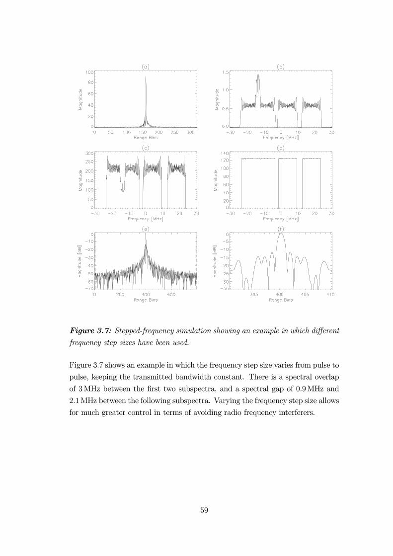
Figure 3.7: Stepped-frequency simulation showing an example in which differentfrequency step sizes have been used.
Figure 3.7 shows an example in which the frequency step size varies from pulse to
pulse, keeping the transmitted bandwidth constant. There is a spectral overlap
of 3MHz between the first two subspectra, and a spectral gap of 0.9MHz and
2.1MHz between the following subspectra. Varying the frequency step size allows
for much greater control in terms of avoiding radio frequency interferers.
59

Figure 3.8: Stepped-frequency simulation showing an example in which differentfrequency step sizes and different transmit bandwidths have been used.
Figure 3.8 shows an example in which the frequency step size varies from pulse
to pulse, and the transmit bandwidth varies from pulse to pulse. There is a
spectral overlap of 1MHz between the first two subspectra, and a spectral gap of
4MHz and 5MHz between the following subspectra. This example illustrates the
flexibility of this stepped-frequency processing method. However, it is important
that the compression filter should be suitably matched to the data in order
successfully to flatten the reconstructed spectrum. Being able to control the
frequency step size and the transmit bandwidth from pulse to pulse offers the
greatest flexibility in terms of notching out RFI.
60
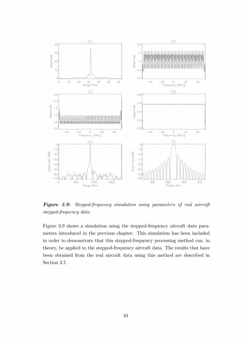
Figure 3.9: Stepped-frequency simulation using parameters of real aircraft
stepped-frequency data.
Figure 3.9 shows a simulation using the stepped-frequency aircraft data para-
meters introduced in the previous chapter. This simulation has been included
in order to demonstrate that this stepped-frequency processing method can, in
theory, be applied to the stepped-frequency aircraft data. The results that have
been obtained from the real aircraft data using this method are described in
Section 3.7.
61
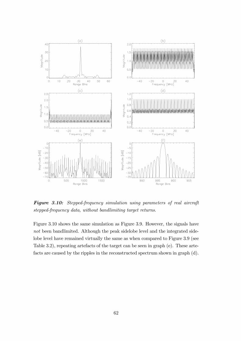
Figure 3.10: Stepped-frequency simulation using parameters of real aircraftstepped-frequency data, without bandlimiting target returns.
Figure 3.10 shows the same simulation as Figure 3.9. However, the signals have
not been bandlimited. Although the peak sidelobe level and the integrated side-
lobe level have remained virtually the same as when compared to Figure 3.9 (see
Table 3.2), repeating artefacts of the target can be seen in graph (e). These arte-
facts are caused by the ripples in the reconstructed spectrum shown in graph (d).
62
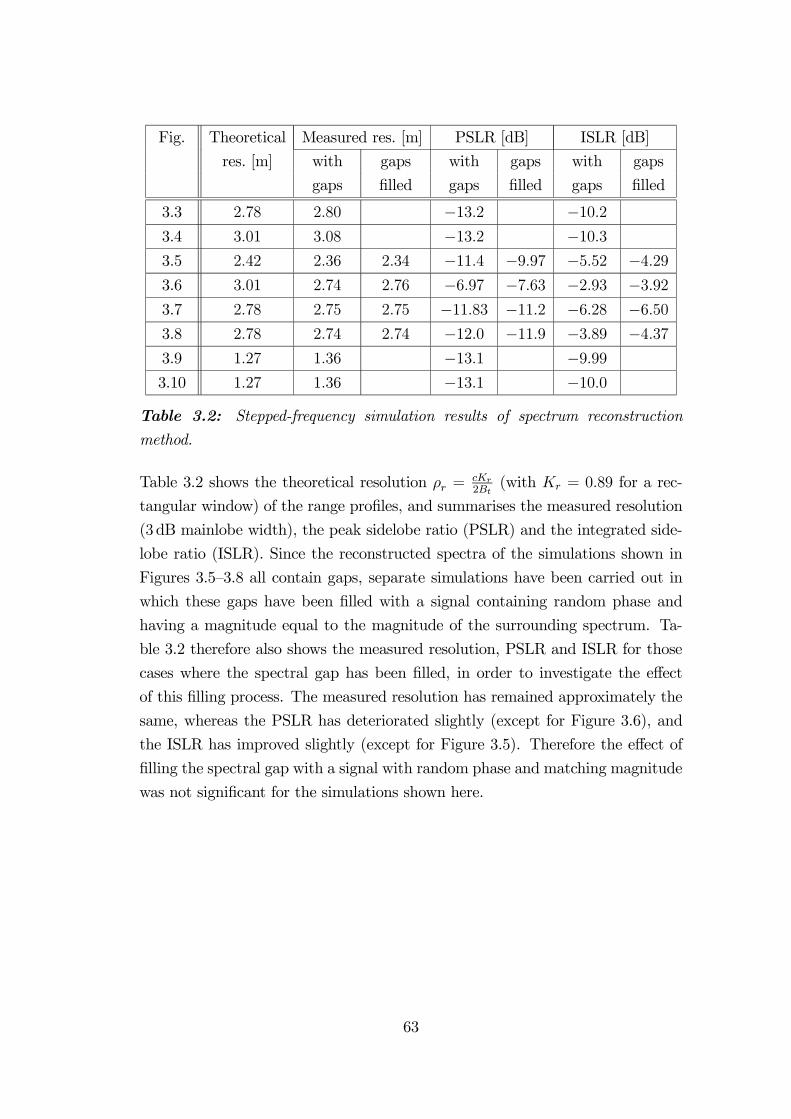
Fig. Theoretical Measured res. [m] PSLR [dB] ISLR [dB]
res. [m] with gaps with gaps with gaps
gaps filled gaps filled gaps filled
3.3 2.78 2.80 −13.2 −10.23.4 3.01 3.08 −13.2 −10.33.5 2.42 2.36 2.34 −11.4 −9.97 −5.52 −4.293.6 3.01 2.74 2.76 −6.97 −7.63 −2.93 −3.923.7 2.78 2.75 2.75 −11.83 −11.2 −6.28 −6.503.8 2.78 2.74 2.74 −12.0 −11.9 −3.89 −4.373.9 1.27 1.36 −13.1 −9.993.10 1.27 1.36 −13.1 −10.0
Table 3.2: Stepped-frequency simulation results of spectrum reconstruction
method.
Table 3.2 shows the theoretical resolution ρr =cKr
2Bt(with Kr = 0.89 for a rec-
tangular window) of the range profiles, and summarises the measured resolution
(3dB mainlobe width), the peak sidelobe ratio (PSLR) and the integrated side-
lobe ratio (ISLR). Since the reconstructed spectra of the simulations shown in
Figures 3.5—3.8 all contain gaps, separate simulations have been carried out in
which these gaps have been filled with a signal containing random phase and
having a magnitude equal to the magnitude of the surrounding spectrum. Ta-
ble 3.2 therefore also shows the measured resolution, PSLR and ISLR for those
cases where the spectral gap has been filled, in order to investigate the effect
of this filling process. The measured resolution has remained approximately the
same, whereas the PSLR has deteriorated slightly (except for Figure 3.6), and
the ISLR has improved slightly (except for Figure 3.5). Therefore the effect of
filling the spectral gap with a signal with random phase and matching magnitude
was not significant for the simulations shown here.
63
3.7 Results Obtained from Real Stepped-Fre-
quency Data of Aircraft
Appendix B shows high-resolution synthetic range profiles of aircraft, which have
been obtained using the IFFT method and the spectrum reconstruction method.
These profiles have been upsampled (using a Shannon interpolator) by a factor
of 20, in order to facilitate better comparison between the profiles obtained from
the two methods. The two graphs in the top row show a zoomed-in portion of
the entire high-resolution synthetic range profile, whereas the two graphs in the
bottom row show a larger portion of the entire profile in order to expose “ghost
targets” adjacent to the main target.
The profiles that have been obtained from both methods look very similar, al-
though this aircraft database is not ideally suited for processing with the spec-
trum reconstruction method for the following reasons:
• The radial velocity is not accurately known. An estimate is calculated byinterpolating the flight path described in the recorded data log file. This
estimate has been used to apply a velocity correction to the datasets shown
in Appendix B.
• The data contains a dc-offset. This offset has been removed by subtractingthe mean from the entire burst.
• The data is not entirely bandlimited. This causes inaccurate compensationat the subspectra boundaries, which in turn causes “ghost” profiles in the
time-domain range profile.
• The radar impulse response is not known. To obtain the compression filterfor these datasets it has been assumed that the radar is ideal and that
there are no non-linearities. Ideally one would like to have the real return
from a point target or corner reflector, and then use that data to create
the compression filter. An attempt has been made to create a compression
filter using an aircraft dataset whose target profile resembles a point target,
in the form of a sharp spike, but the results that have been obtained were
not significantly better.
64
It is encouraging to see that the main profiles of both methods resemble each
other significantly. However, due to the spill-over of target energy, the “ghost
targets” seen in the profiles obtained from the IFFT method are significantly
larger than those seen in the profiles obtained from the spectrum reconstruction
method. This serves to confirm that the spectrum reconstruction method is
the preferred choice when combining stepped-frequencies for SAR processing
applications.
3.8 Conclusions
This chapter has described a frequency-domain method to combine stepped-
frequency waveforms, which entails the reconstruction of the target’s reflectivity
spectrum. This method is fast, since only FFTs and phase multiplications are
used, and it is flexible, because the frequency step size and the transmit band-
width may vary from pulse to pulse within a burst of pulses. This flexibility
offers the opportunity to avoid spectral regions that are highly contaminated
with RFI, thereby reducing the likelihood of receiver saturation.
The spectrum reconstruction method efficiently uses all of the information con-
tained in the stepped-frequency data to produce reliable, high-resolution range
profiles that do not contain any repeating artefacts or “ghost targets”, as long
as great care is invested in the design of the compression filter which smooths
the reconstructed spectrum. It has been demonstrated on simulated data and
on real aircraft data.
65

66

Chapter 4
RFI Suppression for VHF/UHFSAR
4.1 Introduction
Radio frequency interference is a major problem for SAR systems operating
at VHF/UHF-band, because the spectrum is already used extensively by other
services such as television, mobile communications, radio and cellular phones.
Experience with the SASAR system has shown that even in remote locations
the interference power often exceeds receiver noise by many dB, becoming the
limiting factor on system sensitivity and severely degrading the image quality.
RFI suppression is also important when producing interferometric images at
VHF/UHF-band. This is illustrated in Appendix C, which presents the first
interferometric results of the SASAR system. These results have shown that in
order to see fringe patterns in the interferogram, the RFI has to be suppressed.
The previous chapter described how spectral regions which are heavily contam-
inated with RFI can be avoided with the aid of stepped-frequency waveforms.
However, since virtually the entire VHF/UHF spectrum is scattered with inter-
ference spikes, the above technique can only be applied to notch out the most
dominant RFI sources. This chapter addresses other methods that may be used
to suppress the remaining RFI in the received spectrum.
A brief literature review of the approaches to RFI suppression that have been
used successfully in the SAR community is given in Section 4.2. Of these ap-
67
proaches, only the notch filter and the LMS adaptive filter have been imple-
mented here, and these are described in Sections 4.5 and 4.6 respectively. It is
beyond the scope of this thesis to implement all of the RFI suppression methods
mentioned in Section 4.2. Results using both simulated data and real P-band
and VHF-band data are shown and discussed for these two filters.
In addition to assessing the suitability of the notch filter and the LMS adaptive
filter to suppress RFI in P-band and VHF-band images, the original contribu-
tions of this thesis also entail modifications to these filters in order to enhance
their performance. These modifications include the use of a median filter in
order to obtain an approximation to the signal spectrum envelope, which is
then used by the notch filter to identify and remove interference spikes (see Sec-
tion 4.5.2). Furthermore, the notch filter has been efficiently integrated with
the range-compression stage of the range-Doppler SAR processor. Modifications
to the LMS adaptive filter include sweeping the filter through each range line
from both ends and then averaging the two outputs, sweeping the filter through
each range line twice to allow better convergence of the weight vector, and zero-
padding each range line to reduce edge effects (see Section 4.6.2).
Section 4.7 discusses the issue of finding optimal filter parameters. Ideally one
would like to develop a procedure that automatically finds the optimal set of fil-
ter parameters, regardless of the characteristics of the data or the RFI. Another
issue that is addressed in this section is whether the same filter tap weights may
be used over many successive range lines. This is an important issue, because
it might allow the LMS adaptive filter to be re-written in terms of an equiva-
lent transfer function, which would facilitate efficient integration with the range-
Doppler algorithm. This method is also an original contribution of this thesis
and is described in detail in Section 4.8. Finally, Section 4.9 describes a novel
technique for reducing range sidelobes, which arise as an unwanted by-product
of the RFI suppression stage. This technique is demonstrated on simulated data
and also on real P-band and VHF-band data.
The development, coding, simulation and testing of these techniques is the can-
didate’s own work. Some of the material in this chapter has been published in
the Proceedings of COMSIG’98 (Lord and Inggs 1998), Electronics Letters (Lord
and Inggs 1999b) and in the Proceedings of IGARSS’99 (Lord and Inggs 1999a).
68

4.2 Approaches to RFI Suppression
Suppressing radio interference from a received signal essentially involves three
steps (Abend and McCorkle 1995):
1. Finding a model to parameterise the interfering signals;
2. Estimating the parameters of the interfering signals using the measured
data;
3. Using the estimated parameters to suppress the interference in the data.
Modelling the interference environment would ideally include information such
as the statistics on the density of the interference emitters, the identity (type)
of emitters, their effective radiated power, modulation bandwidth, duty factor
and their temporal dependence. The most direct way of achieving this is to
make use of “sniffer” pulses or “listening beforehand” schemes (Abend and Mc-
Corkle 1995). This method is useful for many signal processing methods, but
its effectiveness depends strongly on how long the RFI remains coherent. Most
approaches use a model of the RFI as being a superposition of single sinusoidal
“tones”, and of the wideband signal-plus-system noise as white noise. Surveys
performed by the Grumman E-2C UHF radar (420—450MHz) (Koutsoudis and
Lovas 1995) have shown that 50% of emitters have a spectral bandwidth between
0—50kHz (single channel voice/radio telegraphy), 40% between 50—150kHz and
less than 10% have a bandwidth greater than 150kHz (data communications,
multichannel telephony, etc.) It is important to estimate the modulation time of
the RFI, which is the inverse of the RFI bandwidth, in order to predict whether
the parameters of the modelled sinusoidal interference change across one range
line, so as to deduce whether the tone model of the RFI breaks down. According
to Braunstein et al (Braunstein, Ralston and Sparrow 1994), most RFI has a
modulation time of 5—10µs, which is consistent with an effective bandwidth of a
few hundred kHz or less.
RFI suppression algorithms fall into two classes, namely:
1. Spectral estimation and coherent subtraction approaches;
2. Various filter approaches.
69
The relative merits and disadvantages of these approaches are discussed in the
following subsections. One approach that is not investigated here is the cre-
ation of antenna pattern nulls in the direction of the RFI source as a means
for suppressing the interference. This approach has been addressed by Goris
et al (Goris, Joseph, Hampson and Smits 1999).
4.2.1 Spectral estimation and coherent subtraction ap-
proaches
These approaches have been shown to be extremely effective and powerful to
the extent that the model of RFI as a superposition of sinusoids is true. They
require the estimation of the frequency, phase and amplitude (ω,φ, A) of each
interfering sinusoid, after which the sinusoids are subtracted from the contami-
nated signal. Their performance is excellent in terms of low signal distortion and
good interference suppression. However, their effectiveness is reduced for high
modulation bandwidths, since the parameters change over the record length.
For computational efficiency and effectiveness, these methods must be “tuned”
to use a priori knowledge, such as knowledge of where the FM-broadcast band
is located (Miller, McCorkle and Potter 1995). Furthermore, the parameters of
the tones (especially the phase) must be estimated for every pulse.
Braunstein et al (Braunstein et al. 1994) have achieved very good results us-
ing a maximum likelihood estimate (MLE) approach. For a single sinusoid in
white noise the parameter vector (ω,φ, A) can be found analytically; however for
multiple sinusoids it becomes an extremely difficult nonlinear problem involving
3m variables, where m is the number of sinusoids to be estimated. An efficient
technique of overcoming this problem is to use an iterative algorithm, where the
initial guess of the estimates is iteratively improved. The initial guess may be
obtained from the data spectrum by applying an FFT. Another method would
be to model the RFI, signal and noise as an autoregressive (AR) process (Abend
and McCorkle 1995), (Marple, S. L. Jr. 1987). The estimate x[n] of the nth
sample of the measured data x[n] is given by
x[n] = −p
k=1
a[k]x[n− k] + u[n] (4.1)
where p is the order of the model, indicating that p/2 sinusoids can be estimated,
a[k] are the autoregressive parameters which need to be derived from the mea-
70

sured data, and u[k] is the signal plus noise (without interference). According
to Braunstein et al (Braunstein et al. 1994) the results obtained by using this
method are similar to those obtained by using the MLE method.
Golden et al (Golden, A. Jr., Werness, Stuff, DeGraaf and Sullivan 1995) used
a parametric maximum likelihood (PML) algorithm for the estimation of the
parameters of the RFI tones. This algorithm is also applied to deramp SAR.
It is claimed that 90—95% of the RFI that could have corrupted a SAR image
may be removed. The number of iterations through the PML algorithm at each
threshold is approximately equal to the number of tones being estimated.
Miller et al (Miller et al. 1995) have developed a chirp-least-squares algorithm
with clipping (CLSC). When comparing this method to adaptive FIR filtering
methods, the following advantages are claimed:
• An estimate-and-subtract algorithm provides the narrowest possible stop-
band for a given data length and therefore minimises time-sidelobes.
• The CLSC technique allows iterative, nonlinear signal (target) excision,
which reduces sidelobes and signal loss even further.
• There are no filter edge effects.
This method makes use of a priori knowledge of the RFI environment. A non-
least-squares approach is used to model FM signals, which vary by as much as
75kHz from the centre frequency.
Ferrell (Ferrell 1995) has developed a method which requires 2-D compression of
the SAR image (containing both signal and interference), after which a second
compressed SAR image (containing only interference) is coherently subtracted.
This requires two arrays of data to be collected in an interleaved manner, which
may require the PRF to be increased by a factor of 2. It is claimed that this
method leaves the target and clutter phase history essentially intact.
4.2.2 Filter approaches
A common suppression approach is to examine the spectrum of the contaminated
signal, to identify the interference spikes which are usually many dB larger than
71

the signal, and then to remove these spikes with a notch filter. Although the
notching concept is effective for very narrowband interferers and a small number
of emitters, it can also produce adverse effects on the overall radar system perfor-
mance (Koutsoudis and Lovas 1995), such as reducing image intensity, reducing
range resolution, creating loss in the target’s integrated signal-to-noise ratio and
introducing time-sidelobes.
Koutsoudis and Lovas (Koutsoudis and Lovas 1995) describe an RFI Minimisa-
tion Algorithm developed by Grumman Aerospace Corporation, which is based
on least-mean-squares estimation theory. A single filter is used to achieve both
the interference suppression as well as the equalisation needed to overcome the
distortions caused by the notching function. This method has been tested ex-
tensively using numerous data sets, and excellent performance results have been
obtained for all scenarios.
Buckreuss (Buckreuss 1998) has implemented a notch filter to suppress RFI in
contaminated P-band data. The interferences have been removed to a large
extent, with some sidelobes visible in areas with intense backscatter, as well as
a slight degradation of the contrast.
Abend and McCorkle (Abend and McCorkle 1995) have achieved good results
using an adaptive FIR filter approach. The adaptive filter is an over-determined
system producing an FIR filter with n taps, independent of the number of inter-
fering signals. As opposed to tone extraction methods, this method simultane-
ously eliminates hundreds of narrowband interferers. A low update rate for the
filter tap weights is allowed, since the filter weights were found to be effective for
hundreds of subsequent radar pulses. Furthermore, minimal computational com-
plexity is required, making this a very fast method. An iterative technique has
been used to reduce the range sidelobes caused by the filter’s impulse response.
The adaptive filter is based on an autoregressive (AR) all-pole interference model,
which also models the RFI as sinusoidal tones. However, the sinusoidal model
needs to be valid across the relatively short filter length only. Furthermore the
filter depends only on spectral energy, so the tap weights are not affected by the
phase of the interference tone. A further advantage is that the adaptive filter
“learns” the environment. It is claimed that the interference suppression filter
can be superior to the tone extractor (Abend and McCorkle 1995). A disad-
vantage of using a filter approach is the reduction in record length that arises
because of edge effects.
72
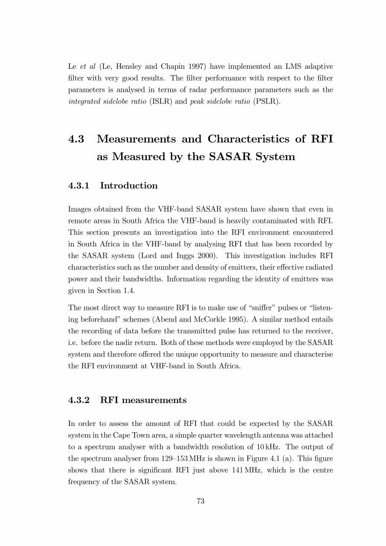
Le et al (Le, Hensley and Chapin 1997) have implemented an LMS adaptive
filter with very good results. The filter performance with respect to the filter
parameters is analysed in terms of radar performance parameters such as the
integrated sidelobe ratio (ISLR) and peak sidelobe ratio (PSLR).
4.3 Measurements and Characteristics of RFI
as Measured by the SASAR System
4.3.1 Introduction
Images obtained from the VHF-band SASAR system have shown that even in
remote areas in South Africa the VHF-band is heavily contaminated with RFI.
This section presents an investigation into the RFI environment encountered
in South Africa in the VHF-band by analysing RFI that has been recorded by
the SASAR system (Lord and Inggs 2000). This investigation includes RFI
characteristics such as the number and density of emitters, their effective radiated
power and their bandwidths. Information regarding the identity of emitters was
given in Section 1.4.
The most direct way to measure RFI is to make use of “sniffer” pulses or “listen-
ing beforehand” schemes (Abend and McCorkle 1995). A similar method entails
the recording of data before the transmitted pulse has returned to the receiver,
i.e. before the nadir return. Both of these methods were employed by the SASAR
system and therefore offered the unique opportunity to measure and characterise
the RFI environment at VHF-band in South Africa.
4.3.2 RFI measurements
In order to assess the amount of RFI that could be expected by the SASAR
system in the Cape Town area, a simple quarter wavelength antenna was attached
to a spectrum analyser with a bandwidth resolution of 10kHz. The output of
the spectrum analyser from 129—153MHz is shown in Figure 4.1 (a). This figure
shows that there is significant RFI just above 141MHz, which is the centre
frequency of the SASAR system.
73
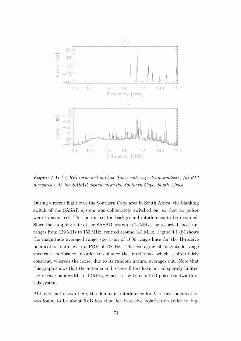
Figure 4.1: (a) RFI measured in Cape Town with a spectrum analyser; (b) RFImeasured with the SASAR system near the Southern Cape, South Africa.
During a recent flight over the Southern Cape area in South Africa, the blanking
switch of the SASAR system was deliberately switched on, so that no pulses
were transmitted. This permitted the background interference to be recorded.
Since the sampling rate of the SASAR system is 24MHz, the recorded spectrum
ranges from 129MHz to 153MHz, centred around 141MHz. Figure 4.1 (b) shows
the magnitude averaged range spectrum of 1000 range lines for the H-receive
polarisation data, with a PRF of 136Hz. The averaging of magnitude range
spectra is performed in order to enhance the interference which is often fairly
constant, whereas the noise, due to its random nature, averages out. Note that
this graph shows that the antenna and receive filters have not adequately limited
the receive bandwidth to 12MHz, which is the transmitted pulse bandwidth of
this system.
Although not shown here, the dominant interference for V-receive polarisation
was found to be about 5dB less than for H-receive polarisation (refer to Fig-
74
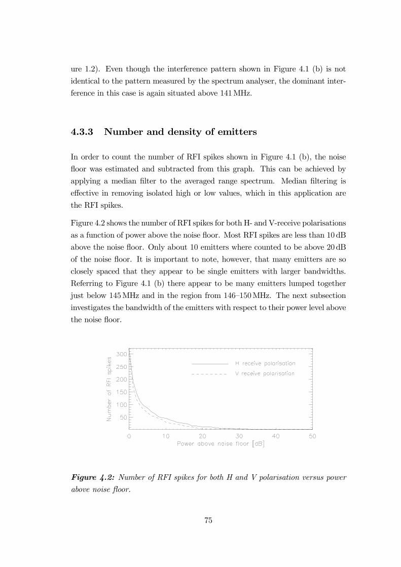
ure 1.2). Even though the interference pattern shown in Figure 4.1 (b) is not
identical to the pattern measured by the spectrum analyser, the dominant inter-
ference in this case is again situated above 141MHz.
4.3.3 Number and density of emitters
In order to count the number of RFI spikes shown in Figure 4.1 (b), the noise
floor was estimated and subtracted from this graph. This can be achieved by
applying a median filter to the averaged range spectrum. Median filtering is
effective in removing isolated high or low values, which in this application are
the RFI spikes.
Figure 4.2 shows the number of RFI spikes for both H- and V-receive polarisations
as a function of power above the noise floor. Most RFI spikes are less than 10dB
above the noise floor. Only about 10 emitters where counted to be above 20dB
of the noise floor. It is important to note, however, that many emitters are so
closely spaced that they appear to be single emitters with larger bandwidths.
Referring to Figure 4.1 (b) there appear to be many emitters lumped together
just below 145MHz and in the region from 146—150MHz. The next subsection
investigates the bandwidth of the emitters with respect to their power level above
the noise floor.
Figure 4.2: Number of RFI spikes for both H and V polarisation versus powerabove noise floor.
75
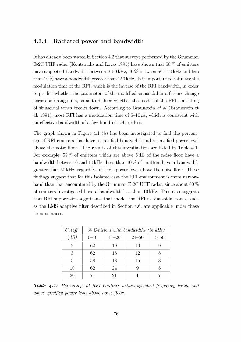
4.3.4 Radiated power and bandwidth
It has already been stated in Section 4.2 that surveys performed by the Grumman
E-2C UHF radar (Koutsoudis and Lovas 1995) have shown that 50% of emitters
have a spectral bandwidth between 0—50kHz, 40% between 50—150kHz and less
than 10%have a bandwidth greater than 150kHz. It is important to estimate the
modulation time of the RFI, which is the inverse of the RFI bandwidth, in order
to predict whether the parameters of the modelled sinusoidal interference change
across one range line, so as to deduce whether the model of the RFI consisting
of sinusoidal tones breaks down. According to Braunstein et al (Braunstein et
al. 1994), most RFI has a modulation time of 5—10µs, which is consistent with
an effective bandwidth of a few hundred kHz or less.
The graph shown in Figure 4.1 (b) has been investigated to find the percent-
age of RFI emitters that have a specified bandwidth and a specified power level
above the noise floor. The results of this investigation are listed in Table 4.1.
For example, 58% of emitters which are above 5dB of the noise floor have a
bandwidth between 0 and 10kHz. Less than 10% of emitters have a bandwidth
greater than 50kHz, regardless of their power level above the noise floor. These
findings suggest that for this isolated case the RFI environment is more narrow-
band than that encountered by the Grumman E-2C UHF radar, since about 60%
of emitters investigated have a bandwidth less than 10kHz. This also suggests
that RFI suppression algorithms that model the RFI as sinusoidal tones, such
as the LMS adaptive filter described in Section 4.6, are applicable under these
circumstances.
Cutoff % Emitters with bandwidths (in kHz)
(dB) 0—10 11—20 21—50 > 50
2 62 19 10 9
3 62 18 12 8
5 58 18 16 8
10 62 24 9 5
20 71 21 1 7
Table 4.1: Percentage of RFI emitters within specified frequency bands andabove specified power level above noise floor.
76

4.4 Description of Real Data Containing RFI
4.4.1 P-band data
Background
The P-band image used in this thesis was generated by the experimental airborne
SAR system E-SAR of the DLR. It shows an area in the vicinity of Weilheim,
Germany, and is displayed in Figure 4.3. The raw data was supplied to the author
by the DLR, Oberpfaffenhofen, Germany, and the processing was done with the
G2 range-Doppler processor developed at the University of Cape Town. Table 4.2
lists the relevant radar parameters of this data set. The RF interference in this
image can be clearly seen as bright lines in the range direction. The interference
is more dominant at the far range due to sensitivity time control (STC). This is
an important issue and is discussed in more detail below.
Figure 4.3: P-band image of the vicinity of Weilheim, Germany, degraded byRF interference. The flight path is along the horizontal axis, with near range
towards the bottom of the image.
77

Centre frequency fc 450MHz
Chirp bandwidth Bt 18MHz
Pulse length Tp 5µs
A/D (complex) sample rate fad 60MHz
Range bins 2048
Table 4.2: Parameters of P-band E-SAR data.
Sensitivity Time Control
Since the received signal power decreases proportionally to the fourth power of
the target range, it is common in radar systems to compensate for this feature by
adjusting the signal strength proportionally. This process increases the dynamic
range of the receiver and is known as sensitivity time control (STC). Before
range compression, the “distortion” of the signal due to the application of STC
is removed by dividing every range line by the appropriate STC curve, to ensure
that the range compression will be applied on the undistorted signal. After range
compression, the STC is again applied to the data to ensure that targets at near
range do not appear brighter than similar targets at far range. Figure 4.4 shows
the STC curve for the P-band data. It should be noted that this curve is not
actually a 4th power curve, but rather an approximately 3rd power curve on
account of antenna effects and SAR azimuth focusing.
Since the signal transmitted by interfering sources is independent of the signal
transmitted by the radar, and since the distance of the interfering sources from
the radar remains approximately constant during one range line, the interference
power received by the radar remains approximately constant and does not decay
across the range window, as does the signal power. One would therefore expect
the STC curve to attenuate the interference signal at near range relative to far
range. This can be seen in Figure 4.5 (a), which shows the real part of a range line
of the P-band data before removal of the STC. It can be seen that the interfering
signal is severely clipped at the far range. This results in the appearance of higher
harmonics in the frequency domain. Furthermore, the signal, which rides on top
of the interference, is therefore also clipped. These aspects cause a degradation
in the final image quality.
It is important to remove the STC before finding the filter weights of the LMS
adaptive filter (see Section 4.6.1), since the interference amplitude ought to re-
78
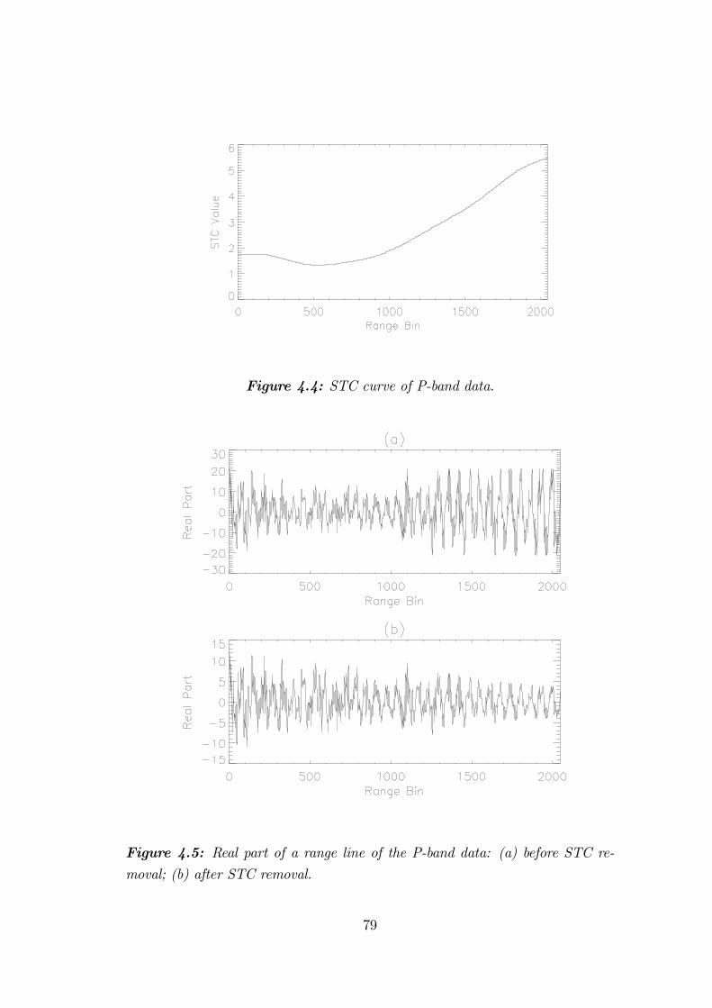
Figure 4.4: STC curve of P-band data.
Figure 4.5: Real part of a range line of the P-band data: (a) before STC re-moval; (b) after STC removal.
79

Figure 4.6: VHF-band image of the vicinity of Upington, South Africa, degradedby RF interference. The flight path is along the horizontal axis, with near range
towards the bottom of the image.
main as constant as possible across the range line. Figure 4.5 (b) shows the same
range line as in Figure 4.5 (a) after STC removal (note different vertical scales).
The interference now seems to decay with range instead of remaining constant;
however, this can be attributed to the clipping described above.
4.4.2 VHF-band data
The VHF-band image used in this thesis was generated by the South African SAR
(SASAR) system. It shows an area in the vicinity of Upington, South Africa,
and is displayed in Figure 4.6. The raw data was processed with the G2 range-
Doppler processor developed at the University of Cape Town (Horrell 1999).
The size of the image is 16.7km in azimuth and 12.8km in range. Table 4.3 lists
the relevant radar parameters of this data set. The RFI in this image is very
Centre frequency fc 141MHz
Chirp bandwidth Bt 12MHz
Pulse length Tp 10.5µs
A/D (complex) sample rate fad 24MHz
Range bins 2048
Table 4.3: Parameters of VHF-band SASAR data.
80
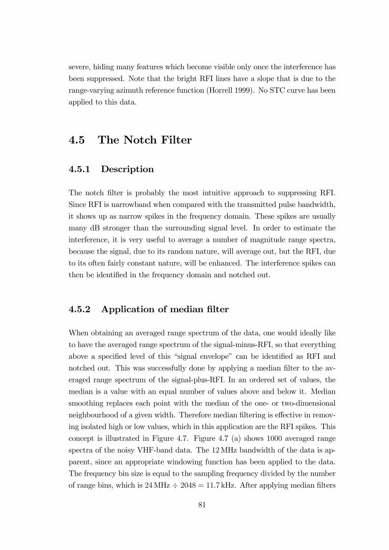
severe, hiding many features which become visible only once the interference has
been suppressed. Note that the bright RFI lines have a slope that is due to the
range-varying azimuth reference function (Horrell 1999). No STC curve has been
applied to this data.
4.5 The Notch Filter
4.5.1 Description
The notch filter is probably the most intuitive approach to suppressing RFI.
Since RFI is narrowband when compared with the transmitted pulse bandwidth,
it shows up as narrow spikes in the frequency domain. These spikes are usually
many dB stronger than the surrounding signal level. In order to estimate the
interference, it is very useful to average a number of magnitude range spectra,
because the signal, due to its random nature, will average out, but the RFI, due
to its often fairly constant nature, will be enhanced. The interference spikes can
then be identified in the frequency domain and notched out.
4.5.2 Application of median filter
When obtaining an averaged range spectrum of the data, one would ideally like
to have the averaged range spectrum of the signal-minus-RFI, so that everything
above a specified level of this “signal envelope” can be identified as RFI and
notched out. This was successfully done by applying a median filter to the av-
eraged range spectrum of the signal-plus-RFI. In an ordered set of values, the
median is a value with an equal number of values above and below it. Median
smoothing replaces each point with the median of the one- or two-dimensional
neighbourhood of a given width. Therefore median filtering is effective in remov-
ing isolated high or low values, which in this application are the RFI spikes. This
concept is illustrated in Figure 4.7. Figure 4.7 (a) shows 1000 averaged range
spectra of the noisy VHF-band data. The 12MHz bandwidth of the data is ap-
parent, since an appropriate windowing function has been applied to the data.
The frequency bin size is equal to the sampling frequency divided by the number
of range bins, which is 24MHz ÷ 2048 = 11.7kHz. After applying median filters
81
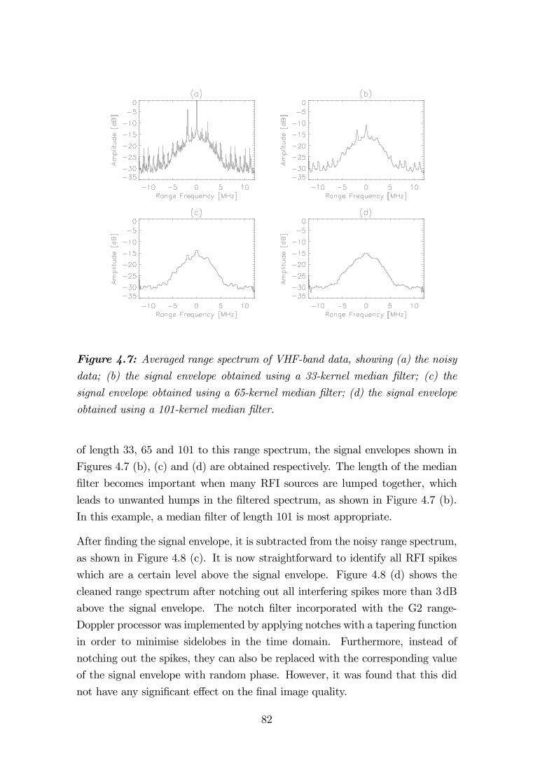
Figure 4.7: Averaged range spectrum of VHF-band data, showing (a) the noisydata; (b) the signal envelope obtained using a 33-kernel median filter; (c) the
signal envelope obtained using a 65-kernel median filter; (d) the signal envelope
obtained using a 101-kernel median filter.
of length 33, 65 and 101 to this range spectrum, the signal envelopes shown in
Figures 4.7 (b), (c) and (d) are obtained respectively. The length of the median
filter becomes important when many RFI sources are lumped together, which
leads to unwanted humps in the filtered spectrum, as shown in Figure 4.7 (b).
In this example, a median filter of length 101 is most appropriate.
After finding the signal envelope, it is subtracted from the noisy range spectrum,
as shown in Figure 4.8 (c). It is now straightforward to identify all RFI spikes
which are a certain level above the signal envelope. Figure 4.8 (d) shows the
cleaned range spectrum after notching out all interfering spikes more than 3dB
above the signal envelope. The notch filter incorporated with the G2 range-
Doppler processor was implemented by applying notches with a tapering function
in order to minimise sidelobes in the time domain. Furthermore, instead of
notching out the spikes, they can also be replaced with the corresponding value
of the signal envelope with random phase. However, it was found that this did
not have any significant effect on the final image quality.
82
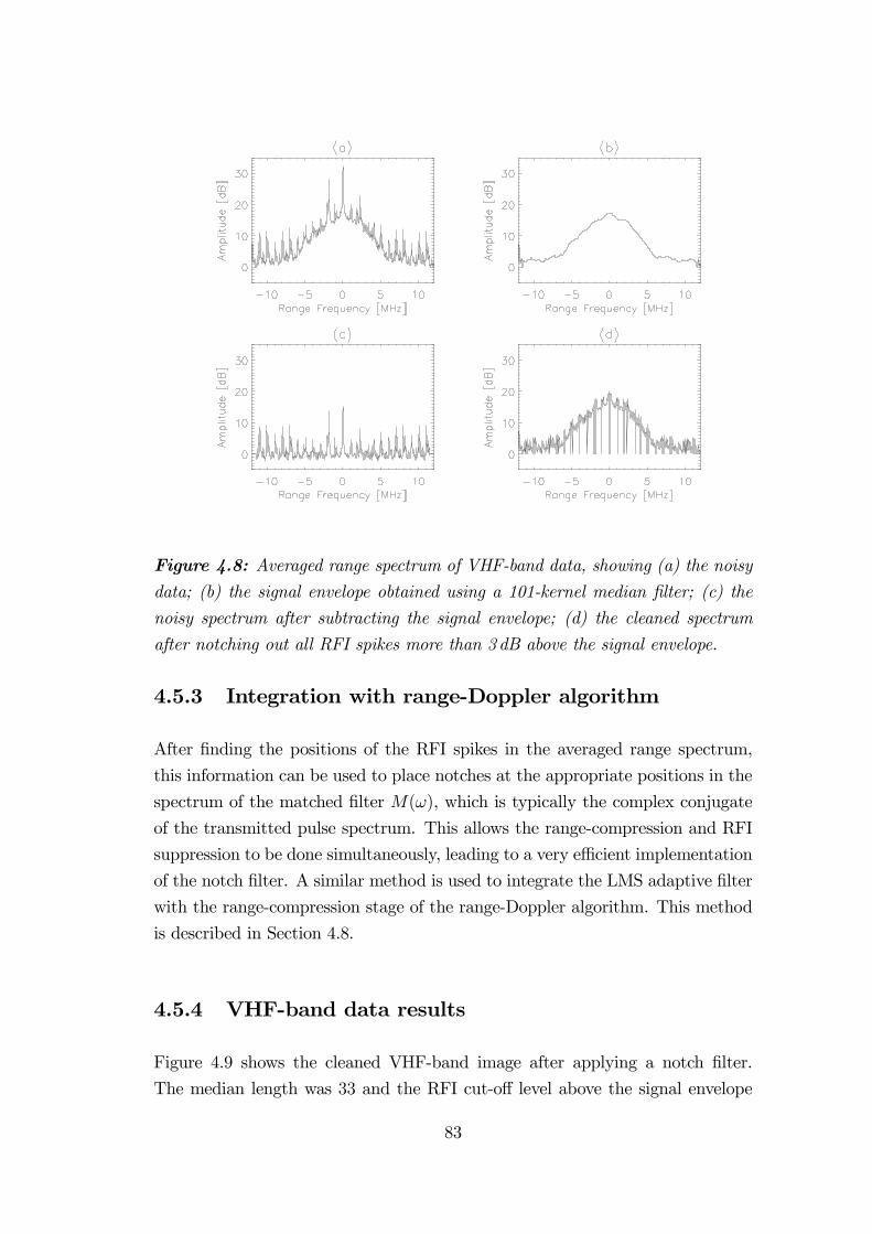
Figure 4.8: Averaged range spectrum of VHF-band data, showing (a) the noisydata; (b) the signal envelope obtained using a 101-kernel median filter; (c) the
noisy spectrum after subtracting the signal envelope; (d) the cleaned spectrum
after notching out all RFI spikes more than 3dB above the signal envelope.
4.5.3 Integration with range-Doppler algorithm
After finding the positions of the RFI spikes in the averaged range spectrum,
this information can be used to place notches at the appropriate positions in the
spectrum of the matched filter M(ω), which is typically the complex conjugate
of the transmitted pulse spectrum. This allows the range-compression and RFI
suppression to be done simultaneously, leading to a very efficient implementation
of the notch filter. A similar method is used to integrate the LMS adaptive filter
with the range-compression stage of the range-Doppler algorithm. This method
is described in Section 4.8.
4.5.4 VHF-band data results
Figure 4.9 shows the cleaned VHF-band image after applying a notch filter.
The median length was 33 and the RFI cut-off level above the signal envelope
83

Figure 4.9: VHF-band image after applying a notch filter to suppress RFI.
Figure 4.10: Optical photo mosaic of VHF-band image.
84
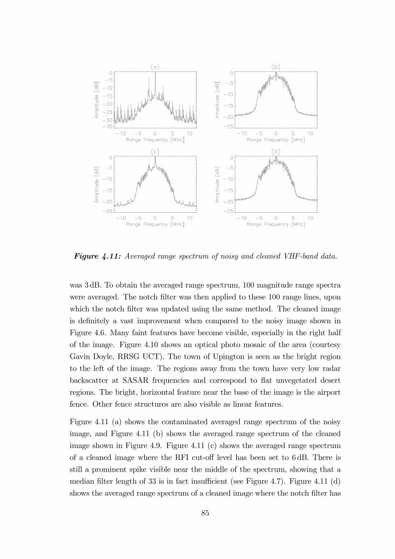
Figure 4.11: Averaged range spectrum of noisy and cleaned VHF-band data.
was 3dB. To obtain the averaged range spectrum, 100 magnitude range spectra
were averaged. The notch filter was then applied to these 100 range lines, upon
which the notch filter was updated using the same method. The cleaned image
is definitely a vast improvement when compared to the noisy image shown in
Figure 4.6. Many faint features have become visible, especially in the right half
of the image. Figure 4.10 shows an optical photo mosaic of the area (courtesy
Gavin Doyle, RRSG UCT). The town of Upington is seen as the bright region
to the left of the image. The regions away from the town have very low radar
backscatter at SASAR frequencies and correspond to flat unvegetated desert
regions. The bright, horizontal feature near the base of the image is the airport
fence. Other fence structures are also visible as linear features.
Figure 4.11 (a) shows the contaminated averaged range spectrum of the noisy
image, and Figure 4.11 (b) shows the averaged range spectrum of the cleaned
image shown in Figure 4.9. Figure 4.11 (c) shows the averaged range spectrum
of a cleaned image where the RFI cut-off level has been set to 6dB. There is
still a prominent spike visible near the middle of the spectrum, showing that a
median filter length of 33 is in fact insufficient (see Figure 4.7). Figure 4.11 (d)
shows the averaged range spectrum of a cleaned image where the notch filter has
85

been updated only every 1000th range line, although only 100 range spectra were
averaged. This verifies that the RFI is fairly constant, and that the notch filter
can be implemented more efficiently by applying it to more range lines than were
used to form the averaged spectrum.
4.6 The LMS Adaptive Filter
4.6.1 Description
Adaptive filters have been widely used in interference suppression applications
(Abend and McCorkle 1995), (Glover, J. R. Jr. 1977), (Le et al. 1997), (Li and
Stoica 1995), (Widrow, Glover, J. R. Jr., McCool, Kaunitz, Williams, Hearn,
Zeidler, Dong, E. Jr. and Goodlin 1975a). In contrast to fixed filters, they have
the desirable property of being able to adjust their own parameters automatically.
Little or no a priori knowledge of the signal or noise characteristics is required.
It is, however, assumed that the interference is sinusoidal. The adaptive filter
relies on a recursive algorithm, which, in a stationary environment, converges
to the optimum Wiener solution (Widrow et al. 1975a). In a non-stationary
environment, the algorithm offers a tracking capability, whereby it can track
time variations in the statistics of the input data.
Figure 4.12 shows a schematic of the LMS adaptive filter as it is used for RF
interference cancelling. It requires a primary input d and a reference input x,
which is obtained by delaying the primary input for some time delay ∆. The
adaptive linear combiner weighs and sums a set of input signals to form an
�
x
y
d ePrimary Input
Reference Input
+
-
�
Delay
LMS Adaptive Filter
W
Figure 4.12: The LMS adaptive filter.
86
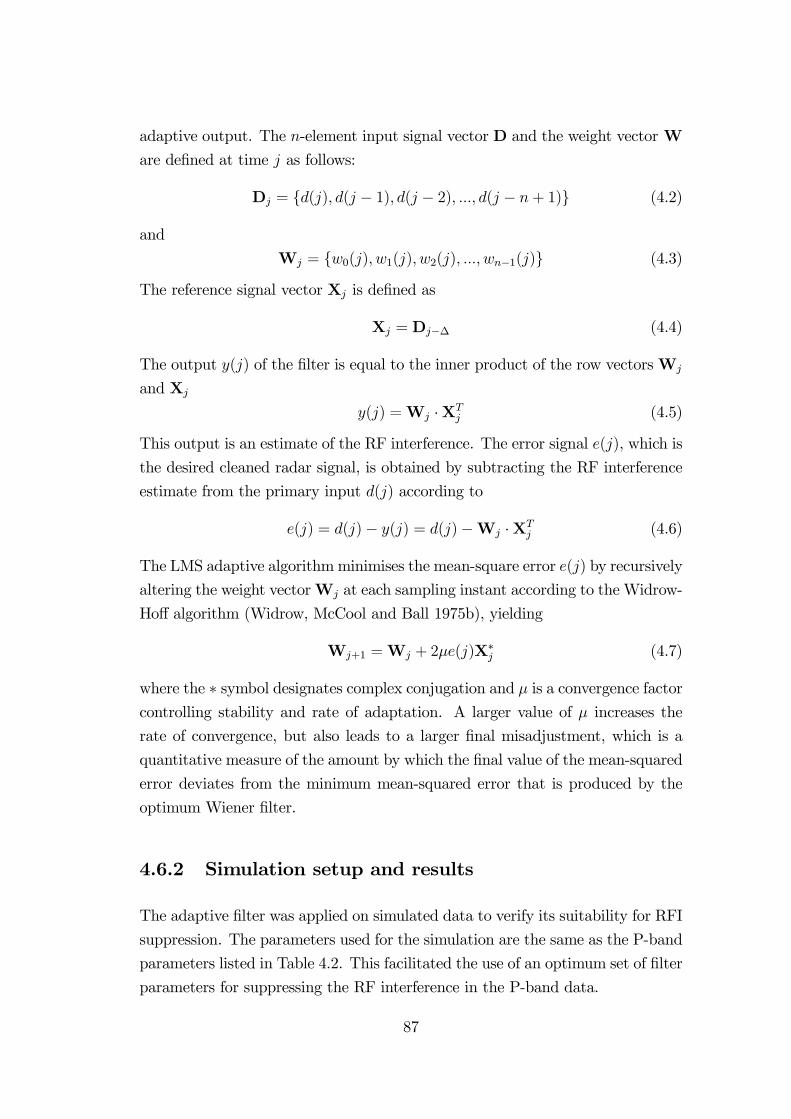
adaptive output. The n-element input signal vector D and the weight vectorW
are defined at time j as follows:
Dj = {d(j), d(j − 1), d(j − 2), ..., d(j − n+ 1)} (4.2)
and
Wj = {w0(j), w1(j), w2(j), ..., wn−1(j)} (4.3)
The reference signal vector Xj is defined as
Xj = Dj−∆ (4.4)
The output y(j) of the filter is equal to the inner product of the row vectorsWj
and Xj
y(j) =Wj ·XTj (4.5)
This output is an estimate of the RF interference. The error signal e(j), which is
the desired cleaned radar signal, is obtained by subtracting the RF interference
estimate from the primary input d(j) according to
e(j) = d(j)− y(j) = d(j)−Wj ·XTj (4.6)
The LMS adaptive algorithmminimises the mean-square error e(j) by recursively
altering the weight vectorWj at each sampling instant according to the Widrow-
Hoff algorithm (Widrow, McCool and Ball 1975b), yielding
Wj+1 =Wj + 2µe(j)X∗j (4.7)
where the ∗ symbol designates complex conjugation and µ is a convergence factorcontrolling stability and rate of adaptation. A larger value of µ increases the
rate of convergence, but also leads to a larger final misadjustment, which is a
quantitative measure of the amount by which the final value of the mean-squared
error deviates from the minimum mean-squared error that is produced by the
optimum Wiener filter.
4.6.2 Simulation setup and results
The adaptive filter was applied on simulated data to verify its suitability for RFI
suppression. The parameters used for the simulation are the same as the P-band
parameters listed in Table 4.2. This facilitated the use of an optimum set of filter
parameters for suppressing the RF interference in the P-band data.
87
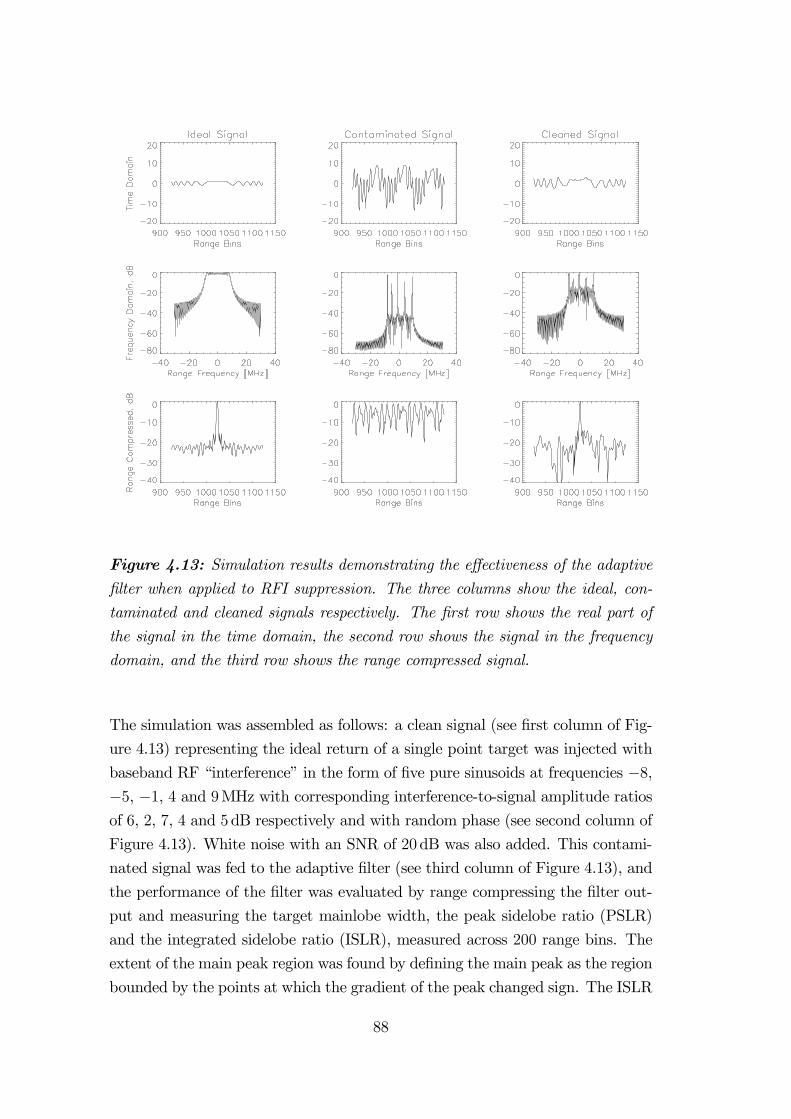
Figure 4.13: Simulation results demonstrating the effectiveness of the adaptivefilter when applied to RFI suppression. The three columns show the ideal, con-
taminated and cleaned signals respectively. The first row shows the real part of
the signal in the time domain, the second row shows the signal in the frequency
domain, and the third row shows the range compressed signal.
The simulation was assembled as follows: a clean signal (see first column of Fig-
ure 4.13) representing the ideal return of a single point target was injected with
baseband RF “interference” in the form of five pure sinusoids at frequencies −8,−5, −1, 4 and 9MHz with corresponding interference-to-signal amplitude ratiosof 6, 2, 7, 4 and 5dB respectively and with random phase (see second column of
Figure 4.13). White noise with an SNR of 20dB was also added. This contami-
nated signal was fed to the adaptive filter (see third column of Figure 4.13), and
the performance of the filter was evaluated by range compressing the filter out-
put and measuring the target mainlobe width, the peak sidelobe ratio (PSLR)
and the integrated sidelobe ratio (ISLR), measured across 200 range bins. The
extent of the main peak region was found by defining the main peak as the region
bounded by the points at which the gradient of the peak changed sign. The ISLR
88
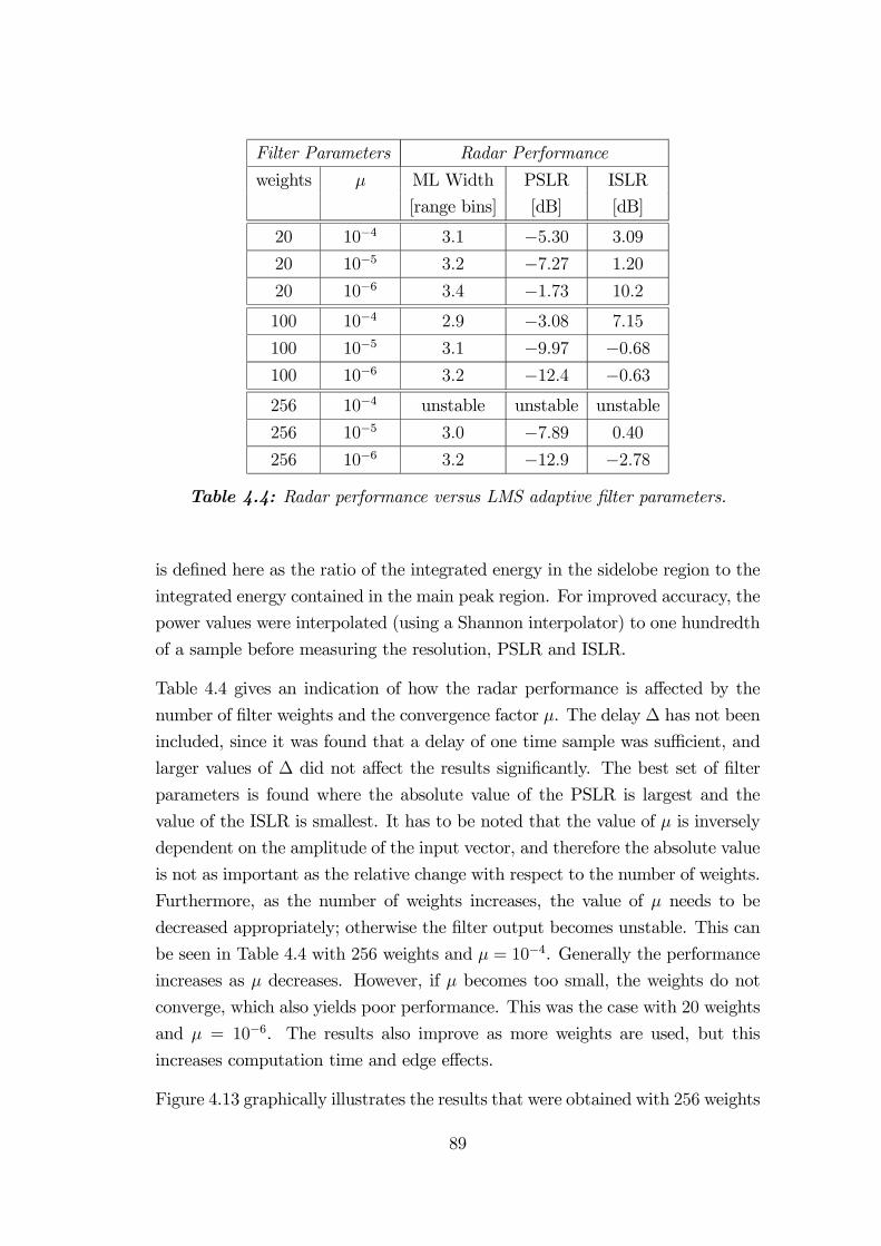
Filter Parameters Radar Performance
weights µ ML Width PSLR ISLR
[range bins] [dB] [dB]
20 10−4 3.1 −5.30 3.09
20 10−5 3.2 −7.27 1.20
20 10−6 3.4 −1.73 10.2
100 10−4 2.9 −3.08 7.15
100 10−5 3.1 −9.97 −0.68100 10−6 3.2 −12.4 −0.63256 10−4 unstable unstable unstable
256 10−5 3.0 −7.89 0.40
256 10−6 3.2 −12.9 −2.78Table 4.4: Radar performance versus LMS adaptive filter parameters.
is defined here as the ratio of the integrated energy in the sidelobe region to the
integrated energy contained in the main peak region. For improved accuracy, the
power values were interpolated (using a Shannon interpolator) to one hundredth
of a sample before measuring the resolution, PSLR and ISLR.
Table 4.4 gives an indication of how the radar performance is affected by the
number of filter weights and the convergence factor µ. The delay ∆ has not been
included, since it was found that a delay of one time sample was sufficient, and
larger values of ∆ did not affect the results significantly. The best set of filter
parameters is found where the absolute value of the PSLR is largest and the
value of the ISLR is smallest. It has to be noted that the value of µ is inversely
dependent on the amplitude of the input vector, and therefore the absolute value
is not as important as the relative change with respect to the number of weights.
Furthermore, as the number of weights increases, the value of µ needs to be
decreased appropriately; otherwise the filter output becomes unstable. This can
be seen in Table 4.4 with 256 weights and µ = 10−4. Generally the performance
increases as µ decreases. However, if µ becomes too small, the weights do not
converge, which also yields poor performance. This was the case with 20 weights
and µ = 10−6. The results also improve as more weights are used, but this
increases computation time and edge effects.
Figure 4.13 graphically illustrates the results that were obtained with 256 weights
89
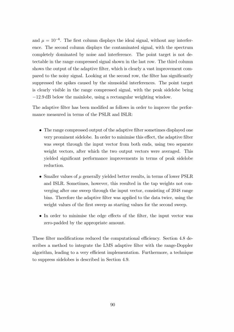
and µ = 10−6. The first column displays the ideal signal, without any interfer-
ence. The second column displays the contaminated signal, with the spectrum
completely dominated by noise and interference. The point target is not de-
tectable in the range compressed signal shown in the last row. The third column
shows the output of the adaptive filter, which is clearly a vast improvement com-
pared to the noisy signal. Looking at the second row, the filter has significantly
suppressed the spikes caused by the sinusoidal interferences. The point target
is clearly visible in the range compressed signal, with the peak sidelobe being
−12.9dB below the mainlobe, using a rectangular weighting window.
The adaptive filter has been modified as follows in order to improve the perfor-
mance measured in terms of the PSLR and ISLR:
• The range compressed output of the adaptive filter sometimes displayed onevery prominent sidelobe. In order to minimise this effect, the adaptive filter
was swept through the input vector from both ends, using two separate
weight vectors, after which the two output vectors were averaged. This
yielded significant performance improvements in terms of peak sidelobe
reduction.
• Smaller values of µ generally yielded better results, in terms of lower PSLRand ISLR. Sometimes, however, this resulted in the tap weights not con-
verging after one sweep through the input vector, consisting of 2048 range
bins. Therefore the adaptive filter was applied to the data twice, using the
weight values of the first sweep as starting values for the second sweep.
• In order to minimise the edge effects of the filter, the input vector waszero-padded by the appropriate amount.
These filter modifications reduced the computational efficiency. Section 4.8 de-
scribes a method to integrate the LMS adaptive filter with the range-Doppler
algorithm, leading to a very efficient implementation. Furthermore, a technique
to suppress sidelobes is described in Section 4.9.
90

Figure 4.14: P-band image after applying the LMS adaptive filter to suppressRF interference.
4.6.3 P-band data resultsFigure 4.14 displays the P-band image after it has been cleaned with a 512-tap
LMS adaptive filter. The RF interference has been suppressed significantly, when
comparing this image with the original image shown in Figure 4.3. Some features
that were hidden by the interference have become visible, although sidelobes of
bright targets have also become more pronounced. This issue is addressed in
Section 4.9, where a technique for reducing these sidelobes is described.
In order to show how successfully the LMS adaptive filter has suppressed the RF
interference, 100 range spectra were averaged before and after RFI suppression.
Averaging a number of range spectra has the effect of enhancing the location and
visibility of the interference spikes, because by coherently averaging the signal
the random component is reduced, whereas the relatively constant interference is
enhanced. However, it must be noted that the radar signal is not random within
the unfocused SAR distance.
Figure 4.15 shows the averaged range spectrum of the noisy data, and the av-
eraged range spectrum after the data has been cleaned with a 512-tap adaptive
filter. The figure shows a large interference spike near the origin, and about 15
smaller spikes on either side of the origin. After the image has been cleaned, the
large interference spike has been reduced by about 12dB, which is a significant
improvement. However, smaller interference spikes are still visible.
91
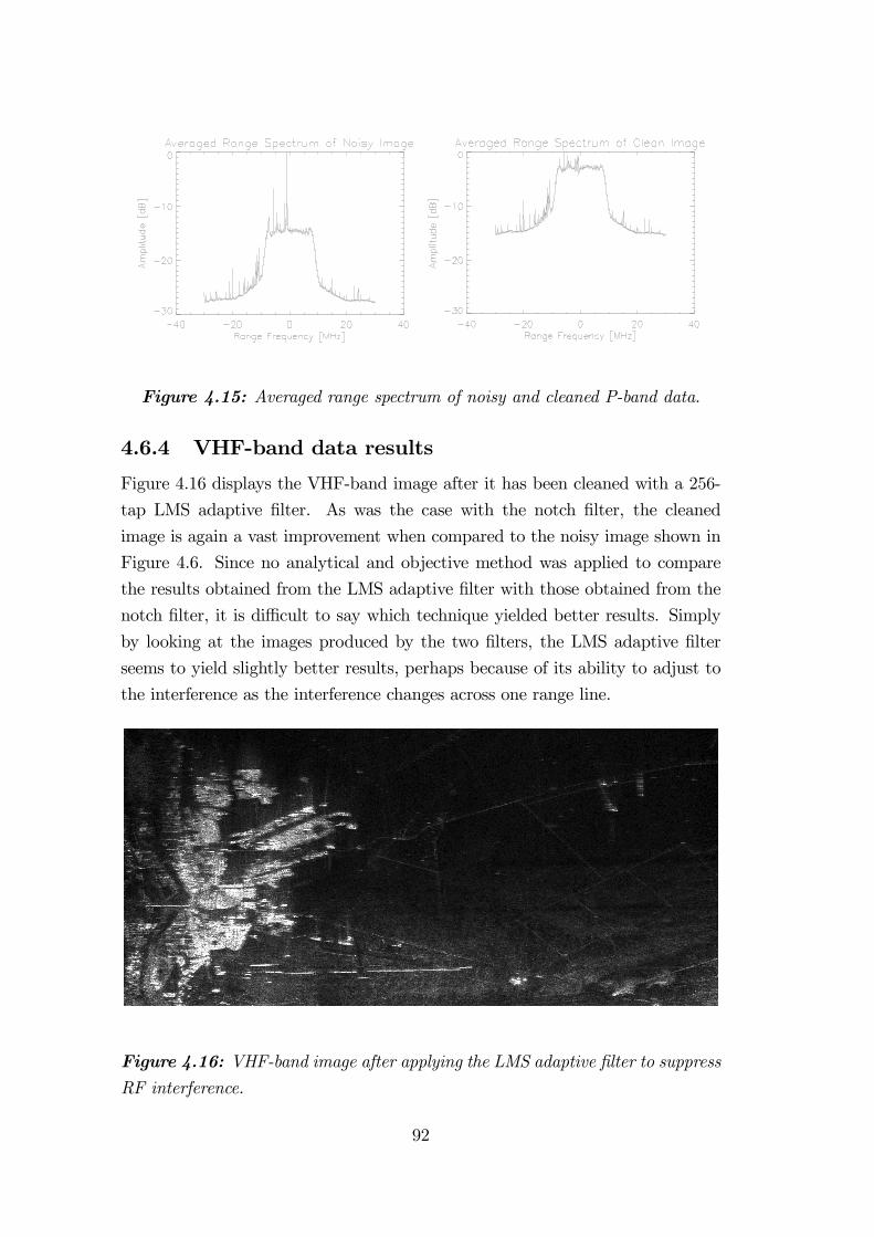
Figure 4.15: Averaged range spectrum of noisy and cleaned P-band data.
4.6.4 VHF-band data results
Figure 4.16 displays the VHF-band image after it has been cleaned with a 256-
tap LMS adaptive filter. As was the case with the notch filter, the cleaned
image is again a vast improvement when compared to the noisy image shown in
Figure 4.6. Since no analytical and objective method was applied to compare
the results obtained from the LMS adaptive filter with those obtained from the
notch filter, it is difficult to say which technique yielded better results. Simply
by looking at the images produced by the two filters, the LMS adaptive filter
seems to yield slightly better results, perhaps because of its ability to adjust to
the interference as the interference changes across one range line.
Figure 4.16: VHF-band image after applying the LMS adaptive filter to suppressRF interference.
92
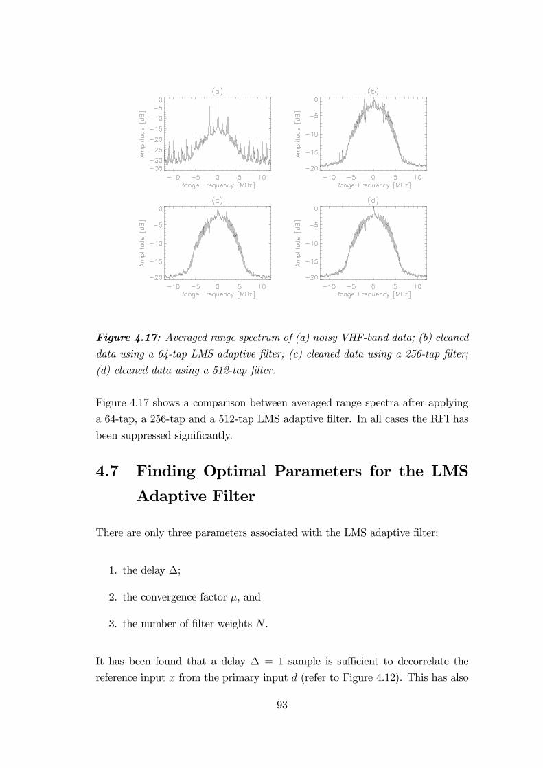
Figure 4.17: Averaged range spectrum of (a) noisy VHF-band data; (b) cleaneddata using a 64-tap LMS adaptive filter; (c) cleaned data using a 256-tap filter;
(d) cleaned data using a 512-tap filter.
Figure 4.17 shows a comparison between averaged range spectra after applying
a 64-tap, a 256-tap and a 512-tap LMS adaptive filter. In all cases the RFI has
been suppressed significantly.
4.7 Finding Optimal Parameters for the LMS
Adaptive Filter
There are only three parameters associated with the LMS adaptive filter:
1. the delay ∆;
2. the convergence factor µ, and
3. the number of filter weights N .
It has been found that a delay ∆ = 1 sample is sufficient to decorrelate the
reference input x from the primary input d (refer to Figure 4.12). This has also
93

been confirmed by other authors (Le et al. 1997). Therefore one only needs to find
the convergence factor µ and the number of filter weights N . Another parameter
that is of interest is the number of range lines across which the same set of filter
weights may be applied successfully. This issue is addressed in Section 4.7.4.
4.7.1 Finding the convergence factor
There is an upper boundary on µ, beyond which the weight-vector mean does
not converge. It is shown by Widrow and Stearns (Widrow and Stearns 1985)
that convergence is guaranteed only if
0 < µ <1
λmax(4.8)
where λmax is the largest eigenvalue of the input correlation matrix. Widrow and
Stearns go on to show that for a transversal adaptive filter, the convergence of
the weight-vector mean is assured by:
0 < µ <1
(N + 1) (signal power)(4.9)
Although this is a more restrictive bound on µ than Equation 4.8, it is much
easier to apply, since the signal power can be estimated more easily than the
eigenvalues of the input correlation matrix.
The closer µ approaches 0, the smaller the convergence error of the weight-vector
becomes when compared with the optimum Wiener solution. It is therefore de-
sirable to make µ as small as possible. This causes the weight-vector to converge
more slowly, which can be remedied by iterating the input vector several times,
and keeping the weights at the end of each iteration as starting values for the
next iteration. If this procedure is done for every range line, the computational
burden increases tremendously, but, as will be shown in Section 4.8, it is intended
to use the same weight-vector for many successive range lines.
The method implemented for finding the weight-vector starts with the first it-
eration by using a value of µ which is a tenth of the maximum value allowed
according to Equation 4.9, and then divides this value of µ by 10 for each suc-
cessive iteration, up to a maximum of 5 iterations. Thus, with each successive
iteration the weight-vector is more finely tuned. The number of iterations and the
division by a factor of 10 is arbitrary; however, good results have been achieved
using these figures. Increasing the number of iterations is wasteful in terms of
94
computation time, and dividing µ by a factor greater than 10 often causes the
weight vector to converge too slowly during the fifth iteration.
4.7.2 Finding a quality index
The most difficult aspect of finding the “optimal” filter parameters lies in finding
a suitable quality index to serve as an objective value that quantifies how “well”
the adaptive filter is doing. One method would be to create simulated data,
containing a point target immersed in RF interference, and then to apply the
adaptive filter to that data. After range-compressing the resulting cleaned signal,
the mainlobe width, the peak sidelobe level and the integrated sidelobe level could
be used as “goodness” parameters (this was demonstrated in Section 4.6.2). The
simulated data should approximate as closely as possible the real dataset to be
cleaned, by having the same number of range bins, the same A/D frequency, the
same chirp bandwidth, et cetera. Most importantly, however, the RFI as well as
the receiver noise should be modelled as accurately as possible. However, as the
RF interference is often unknown, this method is unreliable. In addition, this
method is cumbersome to implement and to automate.
A better way would be to find a quality index using the real dataset. The
LMS adaptive filter tries to minimise the output power (refer to Section 4.6.1),
and therefore it follows that the level of the output power should be a direct
indication of how well the filter is doing. A possible quality index is therefore
the ratio of the output power over the input power, subtracted from unity (the
closer it approaches unity, the better the result). Thus we can define a quality
index η such that
η = 1− Output PowerInput Power
(4.10)
This quality index is intuitive in the sense that the interference spikes become
smaller as the quality index approaches unity. However, when this index is equal
to unity, the output power is zero, which is obviously undesirable, since there is no
signal power left. Therefore one would expect this index to reach some maximum
value, at which point as much interference as possible has been filtered out of
the corrupted signal.
95
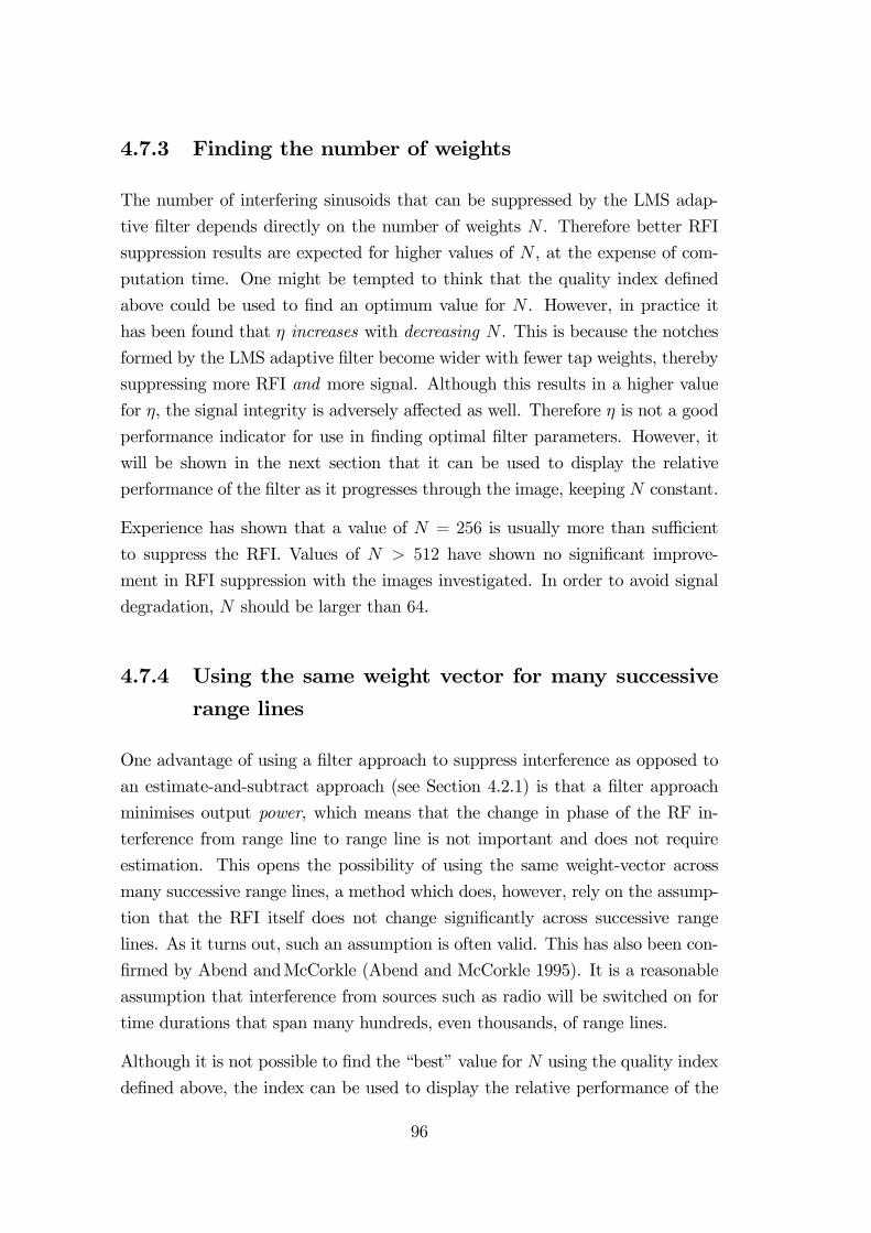
4.7.3 Finding the number of weights
The number of interfering sinusoids that can be suppressed by the LMS adap-
tive filter depends directly on the number of weights N . Therefore better RFI
suppression results are expected for higher values of N , at the expense of com-
putation time. One might be tempted to think that the quality index defined
above could be used to find an optimum value for N . However, in practice it
has been found that η increases with decreasing N . This is because the notches
formed by the LMS adaptive filter become wider with fewer tap weights, thereby
suppressing more RFI and more signal. Although this results in a higher value
for η, the signal integrity is adversely affected as well. Therefore η is not a good
performance indicator for use in finding optimal filter parameters. However, it
will be shown in the next section that it can be used to display the relative
performance of the filter as it progresses through the image, keeping N constant.
Experience has shown that a value of N = 256 is usually more than sufficient
to suppress the RFI. Values of N > 512 have shown no significant improve-
ment in RFI suppression with the images investigated. In order to avoid signal
degradation, N should be larger than 64.
4.7.4 Using the same weight vector for many successive
range lines
One advantage of using a filter approach to suppress interference as opposed to
an estimate-and-subtract approach (see Section 4.2.1) is that a filter approach
minimises output power, which means that the change in phase of the RF in-
terference from range line to range line is not important and does not require
estimation. This opens the possibility of using the same weight-vector across
many successive range lines, a method which does, however, rely on the assump-
tion that the RFI itself does not change significantly across successive range
lines. As it turns out, such an assumption is often valid. This has also been con-
firmed by Abend andMcCorkle (Abend and McCorkle 1995). It is a reasonable
assumption that interference from sources such as radio will be switched on for
time durations that span many hundreds, even thousands, of range lines.
Although it is not possible to find the “best” value for N using the quality index
defined above, the index can be used to display the relative performance of the
96
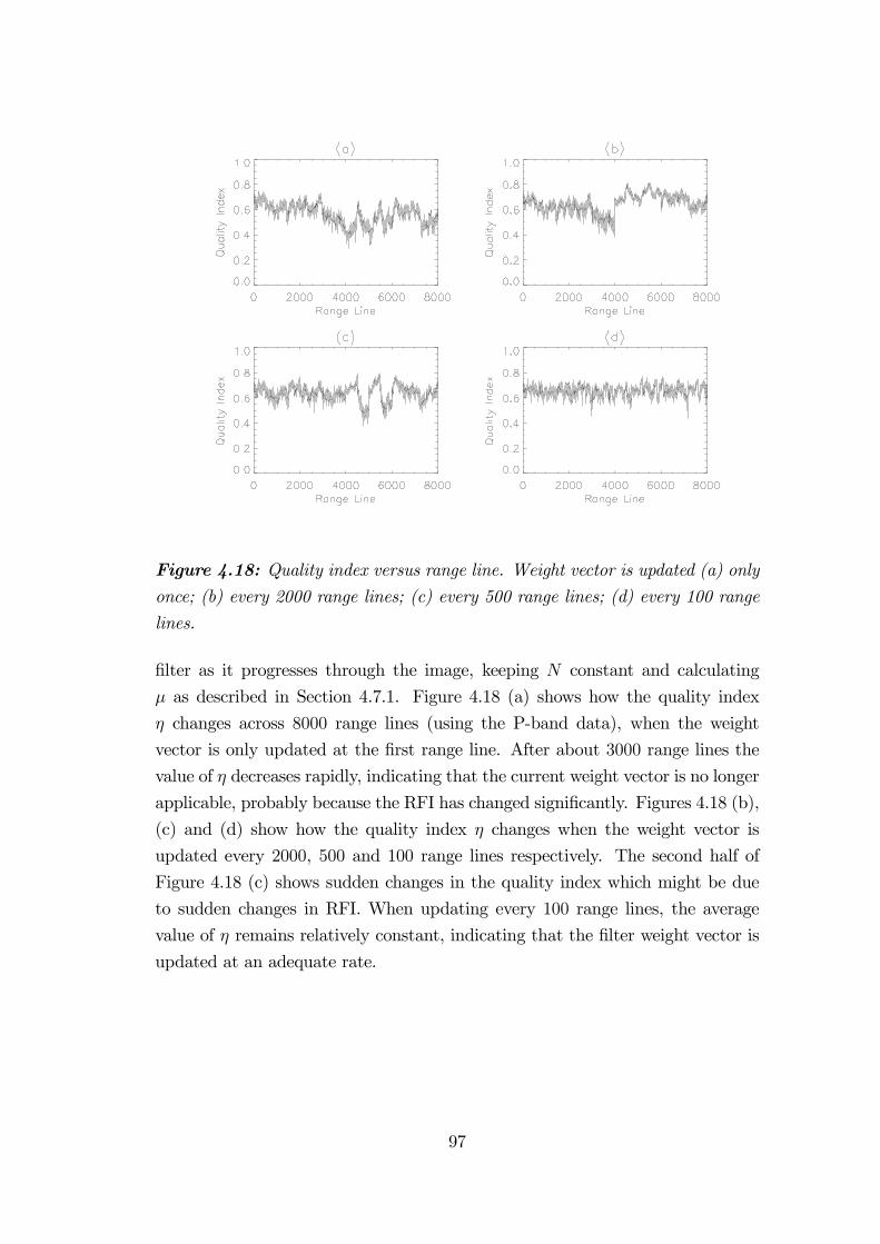
Figure 4.18: Quality index versus range line. Weight vector is updated (a) onlyonce; (b) every 2000 range lines; (c) every 500 range lines; (d) every 100 range
lines.
filter as it progresses through the image, keeping N constant and calculating
µ as described in Section 4.7.1. Figure 4.18 (a) shows how the quality index
η changes across 8000 range lines (using the P-band data), when the weight
vector is only updated at the first range line. After about 3000 range lines the
value of η decreases rapidly, indicating that the current weight vector is no longer
applicable, probably because the RFI has changed significantly. Figures 4.18 (b),
(c) and (d) show how the quality index η changes when the weight vector is
updated every 2000, 500 and 100 range lines respectively. The second half of
Figure 4.18 (c) shows sudden changes in the quality index which might be due
to sudden changes in RFI. When updating every 100 range lines, the average
value of η remains relatively constant, indicating that the filter weight vector is
updated at an adequate rate.
97
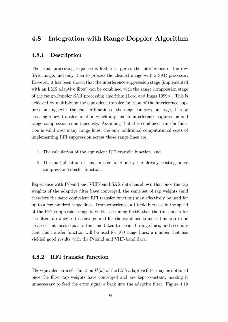
4.8 Integration with Range-Doppler Algorithm
4.8.1 Description
The usual processing sequence is first to suppress the interference in the raw
SAR image, and only then to process the cleaned image with a SAR processor.
However, it has been shown that the interference suppression stage (implemented
with an LMS adaptive filter) can be combined with the range compression stage
of the range-Doppler SAR processing algorithm (Lord and Inggs 1999b). This is
achieved by multiplying the equivalent transfer function of the interference sup-
pression stage with the transfer function of the range compression stage, thereby
creating a new transfer function which implements interference suppression and
range compression simultaneously. Assuming that this combined transfer func-
tion is valid over many range lines, the only additional computational costs of
implementing RFI suppression across those range lines are:
1. The calculation of the equivalent RFI transfer function, and
2. The multiplication of this transfer function by the already existing range
compression transfer function.
Experience with P-band and VHF-band SAR data has shown that once the tap
weights of the adaptive filter have converged, the same set of tap weights (and
therefore the same equivalent RFI transfer function) may effectively be used for
up to a few hundred range lines. From experience, a 10-fold increase in the speed
of the RFI suppression stage is viable, assuming firstly that the time taken for
the filter tap weights to converge and for the combined transfer function to be
created is at most equal to the time taken to clean 10 range lines, and secondly
that this transfer function will be used for 100 range lines, a number that has
yielded good results with the P-band and VHF-band data.
4.8.2 RFI transfer function
The equivalent transfer functionH(ω) of the LMS adaptive filter may be obtained
once the filter tap weights have converged and are kept constant, making it
unnecessary to feed the error signal e back into the adaptive filter. Figure 4.19
98
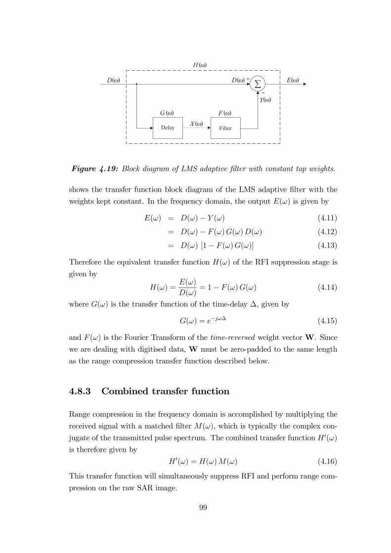
�+
-
Delay Filter
H �( )
�( ) �( )FG
D E
Y
D �( ) �( )
�( )
�( )X
�( )
Figure 4.19: Block diagram of LMS adaptive filter with constant tap weights.
shows the transfer function block diagram of the LMS adaptive filter with the
weights kept constant. In the frequency domain, the output E(ω) is given by
E(ω) = D(ω)− Y (ω) (4.11)
= D(ω)− F (ω)G(ω)D(ω) (4.12)
= D(ω) [1− F (ω)G(ω)] (4.13)
Therefore the equivalent transfer function H(ω) of the RFI suppression stage is
given by
H(ω) =E(ω)
D(ω)= 1− F (ω)G(ω) (4.14)
where G(ω) is the transfer function of the time-delay ∆, given by
G(ω) = e−jω∆ (4.15)
and F (ω) is the Fourier Transform of the time-reversed weight vectorW. Since
we are dealing with digitised data,W must be zero-padded to the same length
as the range compression transfer function described below.
4.8.3 Combined transfer function
Range compression in the frequency domain is accomplished by multiplying the
received signal with a matched filter M(ω), which is typically the complex con-
jugate of the transmitted pulse spectrum. The combined transfer function H (ω)
is therefore given by
H (ω) = H(ω)M(ω) (4.16)
This transfer function will simultaneously suppress RFI and perform range com-
pression on the raw SAR image.
99
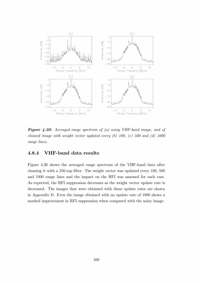
Figure 4.20: Averaged range spectrum of (a) noisy VHF-band image, and of
cleaned image with weight vector updated every (b) 100, (c) 500 and (d) 1000
range lines.
4.8.4 VHF-band data results
Figure 4.20 shows the averaged range spectrum of the VHF-band data after
cleaning it with a 256-tap filter. The weight vector was updated every 100, 500
and 1000 range lines and the impact on the RFI was assessed for each case.
As expected, the RFI suppression decreases as the weight vector update rate is
decreased. The images that were obtained with these update rates are shown
in Appendix D. Even the image obtained with an update rate of 1000 shows a
marked improvement in RFI suppression when compared with the noisy image.
100

4.9 Sidelobe Reduction
4.9.1 Description
Any interference suppressing filter will corrupt the desired signal with sidelobes.
Abend and McCorkle (Abend and McCorkle 1995) have described a sidelobe re-
ducing procedure which has some similarities to the sidelobe reducing procedure
presented here. Figure 4.21 shows a graphical illustration of the technique.
In Figure 4.21 (a) the RFI contaminated signal passes through the LMS adaptive
filter H(ω), yielding a signal free from RFI, but with introduced sidelobes which
are asymmetrical. It is assumed that the RFI suppression is done perfectly, so
that there is no RFI present in the filtered output. In Figure 4.21 (b), the output
from (a) is subtracted from the unfiltered signal, the result of which is passed
again through the LMS adaptive filter, yielding a cleaned signal which contains
only the (negative) sidelobe. It is assumed that the sidelobe embedded in the RFI
�+
-
H �( )
H �( )
H �( )
(a)
(b)
(c) + =
Figure 4.21: Graphical illustration of sidelobe reduction procedure. The largetriangle represents the wanted compressed target, the small triangle the unwanted
sidelobe, and the sinusoidal waveform the unwanted RFI interference.
101
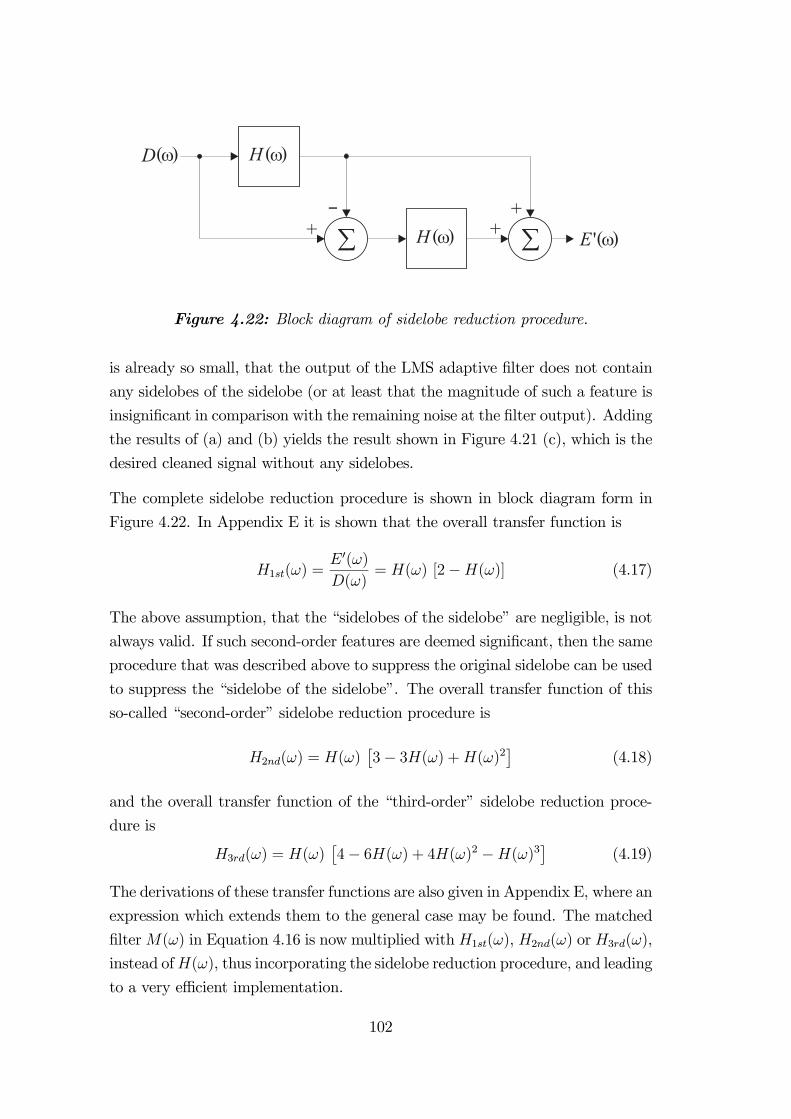
D �( )
�+
-
H �( )�
+
H �( )
+�( )'E
Figure 4.22: Block diagram of sidelobe reduction procedure.
is already so small, that the output of the LMS adaptive filter does not contain
any sidelobes of the sidelobe (or at least that the magnitude of such a feature is
insignificant in comparison with the remaining noise at the filter output). Adding
the results of (a) and (b) yields the result shown in Figure 4.21 (c), which is the
desired cleaned signal without any sidelobes.
The complete sidelobe reduction procedure is shown in block diagram form in
Figure 4.22. In Appendix E it is shown that the overall transfer function is
H1st(ω) =E (ω)
D(ω)= H(ω) [2−H(ω)] (4.17)
The above assumption, that the “sidelobes of the sidelobe” are negligible, is not
always valid. If such second-order features are deemed significant, then the same
procedure that was described above to suppress the original sidelobe can be used
to suppress the “sidelobe of the sidelobe”. The overall transfer function of this
so-called “second-order” sidelobe reduction procedure is
H2nd(ω) = H(ω) 3− 3H(ω) +H(ω)2 (4.18)
and the overall transfer function of the “third-order” sidelobe reduction proce-
dure is
H3rd(ω) = H(ω) 4− 6H(ω) + 4H(ω)2 −H(ω)3 (4.19)
The derivations of these transfer functions are also given in Appendix E, where an
expression which extends them to the general case may be found. The matched
filterM(ω) in Equation 4.16 is now multiplied with H1st(ω), H2nd(ω) or H3rd(ω),
instead ofH(ω), thus incorporating the sidelobe reduction procedure, and leading
to a very efficient implementation.
102

Figure 4.23: Simulation results of sidelobe reduction procedure: (a) RFI conta-minated echo return; (b) filtered echo return with no sidelobe reduction (arrows
point at unwanted sidelobes); (c) filtered echo return with first-order sidelobe re-
duction; (d) filtered echo return with second-order sidelobe reduction.
103

4.9.2 Simulation results
Figure 4.23 summarises simulation results which verify the effectiveness of the
sidelobe reduction procedure. In Figure 4.23 (a) the range-compressed, RFI
contaminated signal is shown. The target is swamped by RFI and cannot be
detected. Figure 4.23 (b) shows the result obtained after cleaning the signal,
with no sidelobe reduction applied. The arrows in the figure point to clearly
visible asymmetric sidelobes. Figure 4.23 (c) and (d) show the cleaned signal with
first-order and second-order sidelobe reduction applied respectively. A marked
reduction in sidelobe levels is evident.
4.9.3 P-band data results
Figure 4.24 (a) displays a zoomed-in portion of the RFI contaminated P-band
image. This region contained especially bright targets, which gave rise to un-
acceptably high sidelobes as depicted in Figure 4.24 (b). After cleaning this
image with the third-order sidelobe reduction procedure, the image shown in
Figure 4.24 (c) was obtained, which is clearly a vast improvement. However,
some of the original interference started appearing again. Thus the original
RFI suppression capability of the filter is compromised by applying the sidelobe
reduction procedure. The sidelobe reduction order to use depends on the bright-
ness of the target. Since the targets displayed in Figure 4.24 were exceptionally
bright, the “sidelobes of the sidelobe” were still clearly visible after applying the
first-order sidelobe reduction procedure. The best results were obtained using
the third-order sidelobe reduction procedure.
4.9.4 VHF-band data results
Figure 4.25 (a) displays a zoomed-in portion of the VHF-band image after it has
been cleaned without any sidelobe reduction. Figure 4.25 (b) shows the same
image after it has been cleaned with a first-order sidelobe reduction procedure.
Again there is a definite improvement in sidelobe levels visible. Applying higher
order sidelobe reduction did not yield any better results.
Experience has shown that applying the sidelobe reduction technique sometimes
reduces the RFI suppression capability of the filter. It is therefore important
to keep the rate at which the filter weights are updated as small as possible, in
order to maximise the amount of RFI suppression.
104
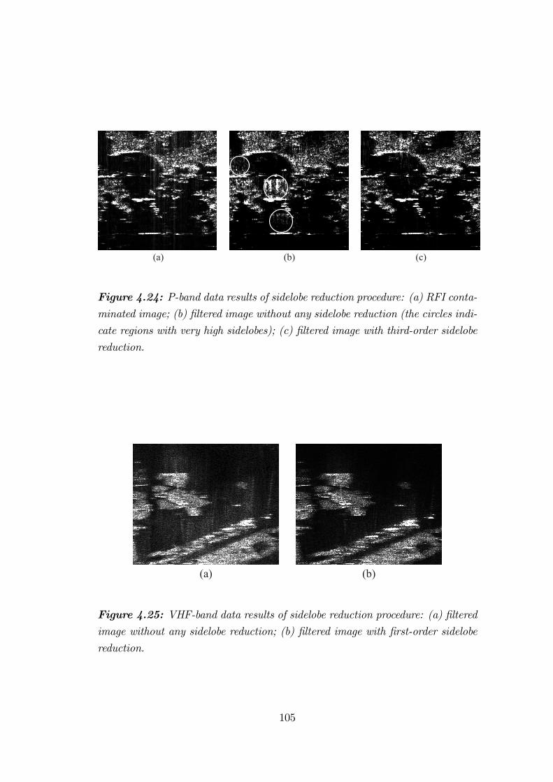
(a) (b) (c)
Figure 4.24: P-band data results of sidelobe reduction procedure: (a) RFI conta-minated image; (b) filtered image without any sidelobe reduction (the circles indi-
cate regions with very high sidelobes); (c) filtered image with third-order sidelobe
reduction.
(a) (b)
Figure 4.25: VHF-band data results of sidelobe reduction procedure: (a) filteredimage without any sidelobe reduction; (b) filtered image with first-order sidelobe
reduction.
105
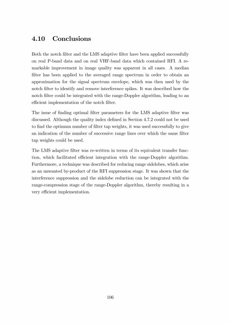
4.10 Conclusions
Both the notch filter and the LMS adaptive filter have been applied successfully
on real P-band data and on real VHF-band data which contained RFI. A re-
markable improvement in image quality was apparent in all cases. A median
filter has been applied to the averaged range spectrum in order to obtain an
approximation for the signal spectrum envelope, which was then used by the
notch filter to identify and remove interference spikes. It was described how the
notch filter could be integrated with the range-Doppler algorithm, leading to an
efficient implementation of the notch filter.
The issue of finding optimal filter parameters for the LMS adaptive filter was
discussed. Although the quality index defined in Section 4.7.2 could not be used
to find the optimum number of filter tap weights, it was used successfully to give
an indication of the number of successive range lines over which the same filter
tap weights could be used.
The LMS adaptive filter was re-written in terms of its equivalent transfer func-
tion, which facilitated efficient integration with the range-Doppler algorithm.
Furthermore, a technique was described for reducing range sidelobes, which arise
as an unwanted by-product of the RFI suppression stage. It was shown that the
interference suppression and the sidelobe reduction can be integrated with the
range-compression stage of the range-Doppler algorithm, thereby resulting in a
very efficient implementation.
106
Chapter 5
Conclusions and Scope forFuture Research
5.1 Conclusions
The objectives of this thesis have been the investigation of the following two
aspects of low-frequency (VHF/UHF) SAR processing:
1. The use of stepped-frequency waveforms to synthesise larger total band-
widths and therefore higher range resolution, and
2. Radio frequency interference (RFI) suppression.
Three methods have been described for processing the stepped-frequency data,
namely an IFFTmethod, a time-domain method and a frequency-domainmethod.
Both the IFFT method and the time-domain method have been found to be un-
suitable for SAR processing applications. The IFFT method suffers from spill-
over of energy into consecutive coarse range bins, which leads to the appearance
of “ghost targets” in the resulting high-resolution range profile. The time-domain
method, although not producing any “ghost targets” in the high-resolution range
profile, is computationally inefficient because of the upsampling requirement of
the narrowband pulses before applying the frequency shift.
These considerations have led to the development of a frequency-domain method,
which efficiently uses all of the information in the narrowband pulses to obtain
107
a high-resolution range profile which does not contain any “ghost targets”. The
execution of the signal processing steps is fast, when compared to the time-
domain implementation, since only FFTs and phase multiplications are required,
and no upsampling of the narrow-bandwidth pulses is necessary. This method
does, however, rely on the proper construction of a compression filter, whose
function it is to compress the data if it has not already been range-compressed,
and also to compensate for amplitude “ripples” at the subspectra boundaries. If
these ripples are not properly compensated, repeating target artefacts become
visible in the time-domain range profile.
This method has been shown to be very flexible. Both the step size and the
transmit bandwidths may vary from pulse to pulse within a burst of pulses. It
has therefore been proposed to make use of this property to avoid transmitting
pulses in spectral regions that have been identified as containing large amounts of
interference. Instead of simply omitting a frequency step which would be heavily
contaminated with RFI, the spectral notches can be made suitably small so as
to notch out as little of the spectrum as possible.
RFI has been shown to be a major problem for SAR systems operating at
VHF/UHF frequencies, since the interference power is often many dB stronger
than the received signal power, thereby causing receiver saturation. Stepped-
frequency waveforms alleviate the problem of receiver saturation, firstly by notch-
ing out spectral regions containing the most dominant interfering sources, and
secondly by allowing the A/D converters to sample with a larger number of bits,
since they need only to sample the instantaneous narrowband pulses. Sampling
with a larger number of bits increases the receiver dynamic range, which reduces
the problem of receiver saturation.
Virtually the whole VHF/UHF spectrum is already in use by other services such
as radio, TV and fixed/mobile communications. It is therefore impossible to
avoid all the spectral regions containing RFI, and therefore other RFI suppression
approaches need to be employed to suppress the remaining RFI in the received
data. Various RFI suppression methods have been investigated. However, only
the notch filter and the LMS adaptive filter have been implemented and applied
on real P-band data obtained from the E-SAR system of the DLR, and on real
VHF-band data obtained from the SASAR system.
108
The notch filter is perhaps the most intuitive approach for the suppression of RFI,
since the interference, which shows up as narrowband spikes in the frequency-
domain, is simply notched out. A median filter has been employed to obtain
an approximation of the signal spectrum envelope, which was then used by the
notch filter to identify and remove interference spikes. The notch filter was ef-
ficiently integrated with the range-compression stage of the range-Doppler SAR
processing algorithm. The LMS adaptive filter was implemented because it re-
ceived favourable review in the literature. Both methods significantly suppressed
the RFI in the real images investigated. In particular, the cleaned VHF images
showed detail that was not visible prior to RFI suppression.
Work done on finding optimal filter parameters for the LMS adaptive filter proved
useful for estimating the number of range lines upon which the LMS adaptive fil-
ter could operate without adaptively changing the filter tap weights. It was found
that the filter tap weights were often valid for several hundred range lines, and
this facilitated the re-writing of the LMS adaptive filter in terms of an equivalent
transfer function, which was then integrated with the range-compression stage of
the range-Doppler SAR processing algorithm. Since the range-compression and
the interference suppression could then be performed simultaneously, and since
the equivalent transfer function of the RFI suppression stage is often effective
for hundreds of range lines, large computational savings could be achieved.
A technique was derived to suppress the unwanted sidelobes that may be pro-
duced by the LMS adaptive filter. This method could also be written in terms
of the equivalent transfer function of the LMS adaptive filter, and this allowed
the sidelobe suppression technique to be integrated with the range-compression
stage of the range-Doppler processor. It was found, however, that the sidelobe
suppression technique compromised the LMS adaptive filter’s ability to suppress
RFI, and therefore the weights had to be updated more frequently. Nevertheless,
significant computational savings could still be achieved.
109

5.2 Future Work
Scope for future work includes:
• Investigating the implications of upgrading a single frequency radar systemto a stepped-frequency system in more detail. More work needs to be car-
ried out on a systems level to calculate the costs involved when upgrading
such a radar system.
• Investigating the issues of more accurate motion compensation and azimuthcompression for widebeam, ultra-wideband, airborne, strip-map SAR. Pos-
sible advantages of applying motion compensation to narrowband stepped-
frequency waveforms need to be investigated.
• Comparing the computational efficiency of the IFFT method, the time-
domain method and the frequency-domain method of processing stepped-
frequency data. Although the time-domain technique has been shown to be
inefficient compared to the frequency-domain technique, more work could
be conducted to quantify this statement.
• Investigating the use of a logarithmic low-noise amplifier. This could allowthe increase of the receiver dynamic range without the need to increase
the number of bits of the A/D converter. The correction of this non-
linearity could be performed before the SAR processing, or before the re-
combination of the sub-bands.
• Investigating backscatter-free data in more detail. Backscatter-free datacan be obtained either by switching the transmitter off completely, or by
recording the pre-nadir return, which entails starting the data recording
process before the transmitted pulse has returned to the receiver. The
SASAR system has already obtained backscatter-free data using both of
these methods. In particular the pre-nadir return data could prove useful
for RFI suppression, since the RFI in the pre-nadir return data would
be very similar to the RFI in the remainder of the range line containing
backscatter data.
• Investigating the calibration degradation of the implemented RFI suppres-sion technique. If the V-polarisation and H-polarisation RFI signals are
different, the polarimetric calibration accuracy will also be degraded.
110
• Investigating the effect of tapering notches on mainlobe width and side-lobe levels. In Section 4.5.2 it has been mentioned that the notches in
the frequency-domain have been tapered in order to reduce time-domain
sidelobes. However, more work could be conducted to show the effects of
various degrees of tapering.
• Optimising the filter parameters of the LMS adaptive filter. This topic hasalready been addressed in Chapter 4, but more work could be conducted
to investigate adaptively changing the parameters of the filter (such as the
number of tap weights or the convergence factor) as it sweeps through the
image.
• Investigating the problem of RFI suppression by making use of informationtheory. The two methods implemented in this thesis, namely the notch fil-
ter and the LMS adaptive filter, could be classified as adhoc approaches,
which do not efficiently use all of the information that is contained in the
RFI contaminated images. This would require more work to be conducted
in analysing the characteristics of the interference, such as frequency spac-
ing, bandwidth, polarisation, etc. This issue is currently being addressed
by the candidate at UCT.
• Development of more quantified methods to evaluate the performance ofRFI suppression techniques.
• Obtaining data from different sensors at different frequencies. Since the
RFI encountered at different frequencies can be very different, one would
have to investigate data at different centre frequencies in order to develop
a strategy for automatically suppressing RFI in various scenarios.
111

112

Appendix A
IFFT Method Simulation Results
This appendix lists the point target simulation results of the IFFT method for
producing synthetic range profiles from stepped-frequency data. Refer to Sec-
tion 2.5.2 for a discussion regarding these results.
Table A.1 lists the relevant parameters for each simulation. These parameters
were chosen to correspond with the VHF-band SASAR system, which has a cen-
tre frequency fc = 141MHz and which transmits linear FM chirps with a pulse
length of Tp = 10µs and a bandwidth of Bt = 12MHz sampled at fad = 24MHz.
Therefore, for every simulation, n = 4 narrowband pulses were transmitted with
Btx = 12MHz, Tp = 10µs and a combined centre frequency of fc = 141MHz,
which is the average between the first centre frequency and the last centre fre-
quency. Note therefore that the first centre frequency of the simulations shown
in Figures A.4 and A.6 are different from those of the other simulations due to
the different frequency step size.
The pulses were range-compressed before applying the IFFT. The theoretical
resolution for the narrowband pulses is given by ρr =cKr
2Btx= 11.1m, with Kr =
0.89 for rectangular window weighting. The percentage overlap between SRPs
of successive coarse range bins is given by Equation 2.16.
Each figure in this appendix shows the following graphs:
(a) Magnitude of range-compressed target return, first frequency step.
(b) Nine coarse range bins centred around the peak of the target return shown
in (a). The complex data has been upsampled (using a Shannon interpo-
lator) by a factor of 100.
113

(c) A dB plot of the entire synthetic range profile, with appropriate overlapping
of range profiles of neighbouring coarse range bins.
(d) Magnitude plot of a zoomed-in portion of the region centred around the
peak of the synthetic range profile. The complex data has been upsampled
by a factor of 100. The range extent shown here is the same as that shown
in (b), in order to illustrate the increase in range resolution.
Fig. A.1 Fig. A.2 Fig. A.3 Fig. A.4 Fig. A.5 Fig. A.6
f0 [MHz] 123 123 123 132 123 132
∆f [MHz] 12 12 12 6 12 6
fad [MHz] 12 12 12 12 24 24
ws [m] 12.5 12.5 12.5 25.0 12.5 25.0
Bin spacing [m] 12.5 12.5 12.5 12.5 6.25 6.25
% overlap none none none 50% 50% 75%
Number of targets 1 2 2 1 1 1
Table A.1: Stepped-frequency simulation parameters of IFFT method.
114

Figure A.1: Simulation result of IFFT method, with no overlap between suc-cessive SRPs. See beginning of appendix for details.
Figure A.1 shows the simulation of a single point target. There is no overlap be-
tween successive range profiles. Comparing Figures A.1 (b) and (d), the fourfold
increase in range resolution can be observed.
115

Figure A.2: Simulation result of IFFT method, showing the return from 2
point targets, which are both positioned in one coarse range bin. See beginning of
appendix for details.
Figure A.2 shows the same simulation as Figure A.1. However, the return from
2 point targets is measured. The point targets are spaced 6m apart, which
is less than the 11.1m resolution associated with each narrowband pulse, and
therefore Figure A.2 (b) appears to show only one point target. Furthermore,
both targets were centred in one coarse range bin. After IFFT processing, the
two point targets are clearly visible, as can be seen in Figure A.2 (d). Note that
the sidelobes have increased, compared to the previous simulation. This can be
attributed to signal energy leaking into neighbouring coarse range bins.
116

Figure A.3: Simulation result of IFFT method, with the 2 point targets be-
ing positioned in neighbouring coarse range bins. See beginning of appendix for
details.
Figure A.3 shows the same simulation as Figure A.2. However, now the two point
targets are positioned in neighbouring coarse range bins. From Figure A.3 (d)
it appears as though three point targets are present. This is because the signal
energy of the first point target is nearly equally divided between two neighbouring
coarse range bins, whereas most of the signal energy from the second point target
is contained in only one coarse range bin.
117
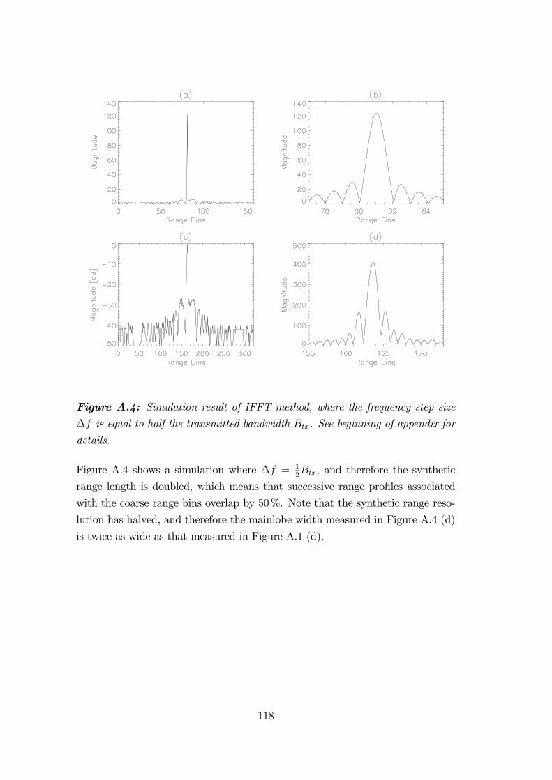
Figure A.4: Simulation result of IFFT method, where the frequency step size∆f is equal to half the transmitted bandwidth Btx. See beginning of appendix for
details.
Figure A.4 shows a simulation where ∆f = 12Btx, and therefore the synthetic
range length is doubled, which means that successive range profiles associated
with the coarse range bins overlap by 50%. Note that the synthetic range reso-
lution has halved, and therefore the mainlobe width measured in Figure A.4 (d)
is twice as wide as that measured in Figure A.1 (d).
118

Figure A.5: Simulation result of IFFT method, where the sample frequency fadis equal to twice the transmitted bandwidth Btx. See beginning of appendix for
details.
Figure A.5 shows a simulation where fad = 2Btx. The synthetic range length
is still the same. However, the coarse range bins are sampled at twice the rate,
causing successive range profiles to overlap by 50%. Since the target energy is
now spread over more than one coarse range bin, there are repeated artefacts of
the target in the combined range profile.
119

Figure A.6: Simulation result of IFFT method, where the frequency step size∆f is equal to half the transmitted bandwidth Btx, and the sample frequency fadis equal to twice the transmitted bandwidth Btx. See beginning of appendix for
details.
Figure A.6 shows a simulation where ∆f = 12Btx and fad = 2Btx, causing succes-
sive range profiles to overlap by 75%. No repeated target artefacts can be seen as
in the previous simulation. However, it has been observed that performing this
simulation with two point targets in neighbouring range bins, as in Figure A.3,
also produces range profiles displaying three point targets.
120

Appendix B
Synthetic Range Profiles ofAircraft
This appendix shows high-resolution synthetic range profiles of aircraft, which
have been obtained using the IFFT method and the spectrum reconstruction
method. All profiles have been upsampled by a factor of 20, in order to facilitate
better comparison between the profiles obtained from the two methods.
The two graphs in the top row (refer to Figures B.1—B.4) show a zoomed-in por-
tion of the entire high-resolution synthetic range profile. For the IFFT method,
this is the synthetic range profile (SRP) obtained when taking an inverse FFT
across all frequency steps in the range bin containing the peak value. For all
examples shown in this appendix, the profiles obtained from the two methods
look very similar.
The two graphs in the bottom row (refer to Figures B.1—B.4) show a larger
portion of the entire high-resolution synthetic range profile, in order to expose
“ghost targets” adjacent to the main target. For the IFFT method, this portion
represents three consecutive SRPs, which have been obtained by taking an inverse
FFT across all frequency steps in the range bin containing the peak value, and
in the range bins adjacent to the bin containing the peak value. For all examples
shown in this appendix, the “ghost targets” of the IFFT method are much more
significant than those of the spectrum reconstruction method.
Further discussions concerning these graphs are given in Section 3.7 of Chapter 3.
121
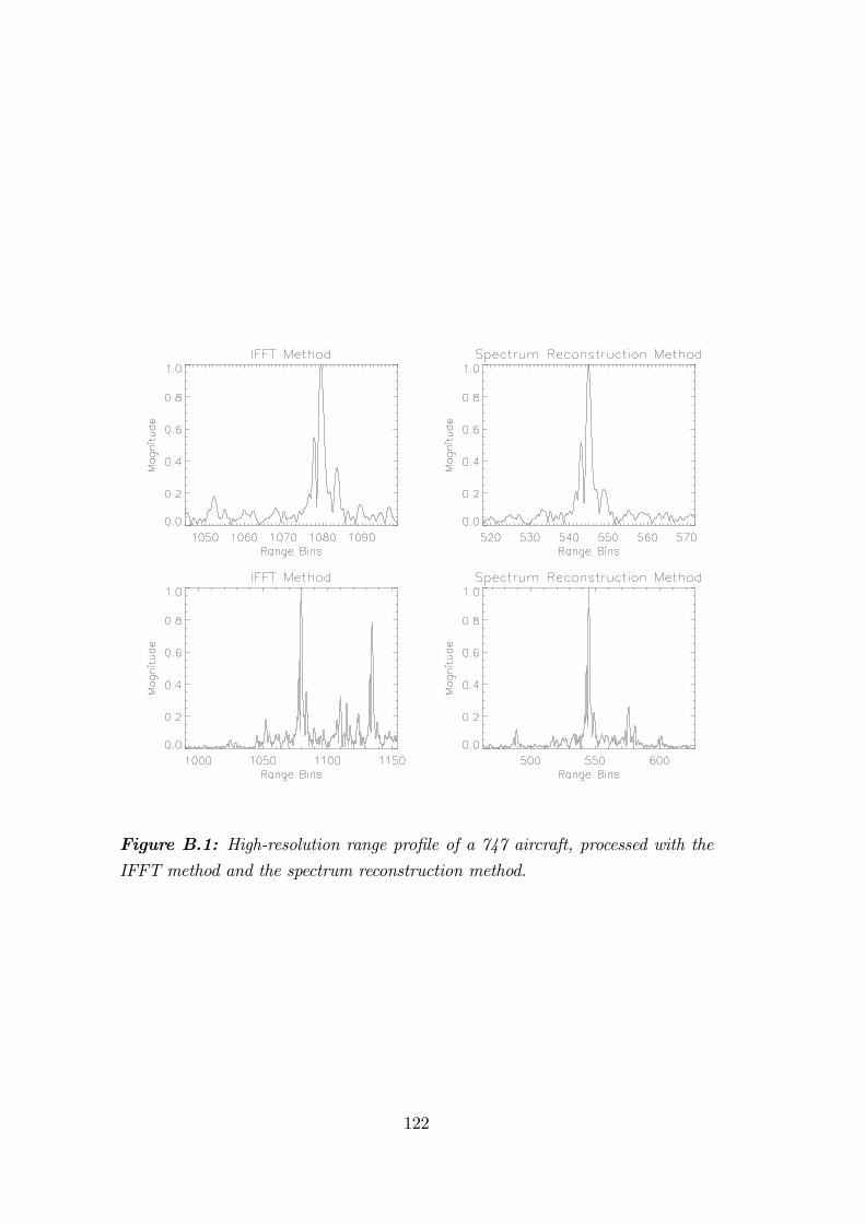
Figure B.1: High-resolution range profile of a 747 aircraft, processed with theIFFT method and the spectrum reconstruction method.
122
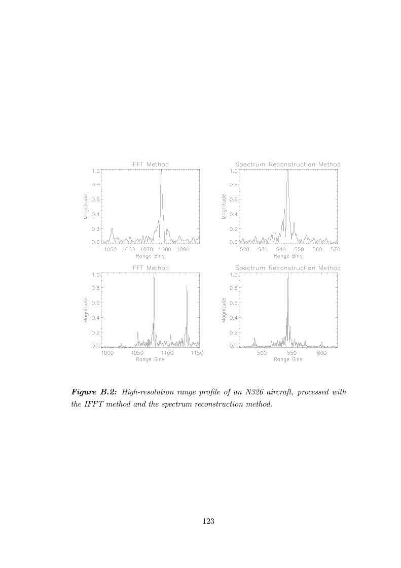
Figure B.2: High-resolution range profile of an N326 aircraft, processed withthe IFFT method and the spectrum reconstruction method.
123

Figure B.3: High-resolution range profile of a King Air B200 aircraft, processedwith the IFFT method and the spectrum reconstruction method.
124

Figure B.4: High-resolution range profile of a Messer Bolkow aircraft, processedwith the IFFT method and the spectrum reconstruction method.
125

126
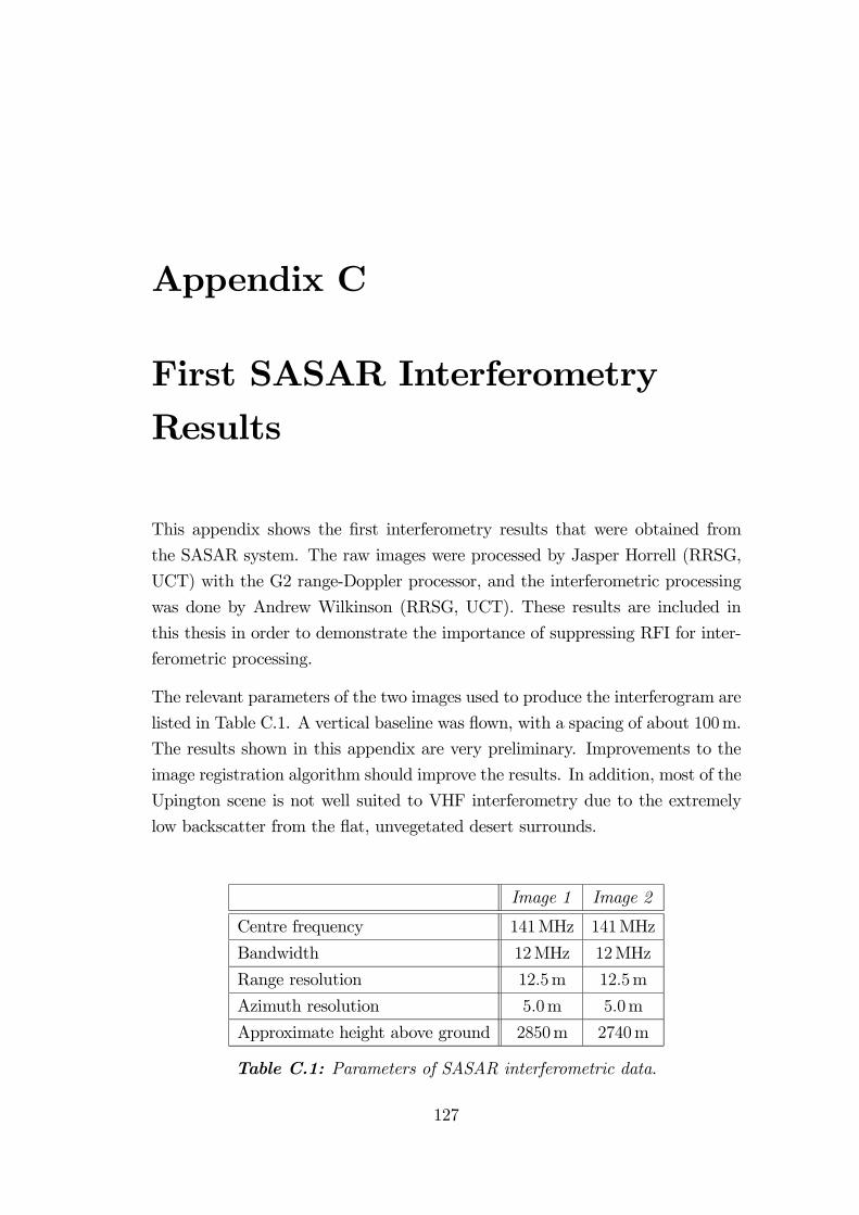
Appendix C
First SASAR InterferometryResults
This appendix shows the first interferometry results that were obtained from
the SASAR system. The raw images were processed by Jasper Horrell (RRSG,
UCT) with the G2 range-Doppler processor, and the interferometric processing
was done by Andrew Wilkinson (RRSG, UCT). These results are included in
this thesis in order to demonstrate the importance of suppressing RFI for inter-
ferometric processing.
The relevant parameters of the two images used to produce the interferogram are
listed in Table C.1. A vertical baseline was flown, with a spacing of about 100m.
The results shown in this appendix are very preliminary. Improvements to the
image registration algorithm should improve the results. In addition, most of the
Upington scene is not well suited to VHF interferometry due to the extremely
low backscatter from the flat, unvegetated desert surrounds.
Image 1 Image 2
Centre frequency 141MHz 141MHz
Bandwidth 12MHz 12MHz
Range resolution 12.5m 12.5m
Azimuth resolution 5.0m 5.0m
Approximate height above ground 2850m 2740m
Table C.1: Parameters of SASAR interferometric data.
127

Figure C.3 shows the correlation image that was formed from the two images
shown in Figures C.1 and C.2. These images were first cleaned with a notch
filter. The correlation image shows a high degree of coherence (about 0.90) in
the top left-hand corner. Generally the town areas and fences provide the regions
of highest coherence. Fringes are clearly visible in the top left-hand area in the
interferogram shown in Figure C.5, which is a zoomed-in portion of the interfer-
ogram shown in Figure C.4. The fringes are not parallel to the flight path, which
runs along the bottom of the image, because the flight paths were not parallel
to each other and this effect has not been corrected here. Figure C.6 shows
the flattened interferogram obtained after removing the flat earth component.
Interesting phase fringes can now be observed, which are hopefully related to
the region’s topography. More work needs to be done to interpret these fringes
correctly.
The RFI contaminated images are shown in Figures C.7 and C.8, and the result-
ing correlation image is shown in Figure C.9. It contains bright lines in the range
direction, which correspond to the RF interference, which is many dB stronger
than the signal. However, there is no apparent signal correlation between the two
images. No fringes are detectable in the interferogram shown in Figure C.10, nor
in the enlarged interferogram of Figure C.11, or in the flattened interferogram
shown in Figure C.12. This verifies the importance of suppressing RFI when
doing interferometric processing.
More recent interferometric results from the SASAR system are shown in Fig-
ures C.13 to C.16. Figure C.13 shows two cleaned magnitude images of the
Hermanus area near the Southern Cape in South Africa, separated by a vertical
baseline of about 100m. Figure C.14 shows the relevant correlation image. A
high degree of coherence is visible, corresponding to the bright regions of the
magnitude images. Figures C.15 and C.16 show the interferogram and flattened
interferogram respectively. When comparing the flattened interferogram with
the magnitude images, a correlation between the fringe pattern and the region’s
topography is already apparent. However, more work needs to be conducted
with the generation and interpretation of these interferograms.
128
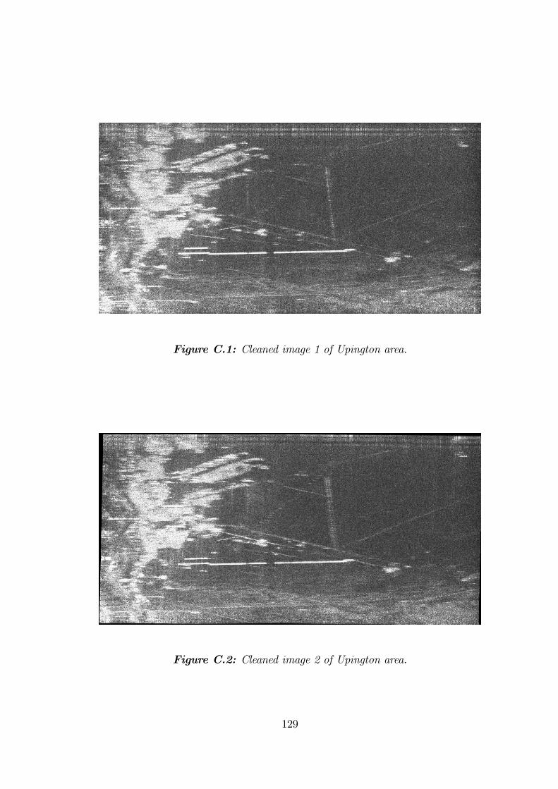
Figure C.1: Cleaned image 1 of Upington area.
Figure C.2: Cleaned image 2 of Upington area.
129
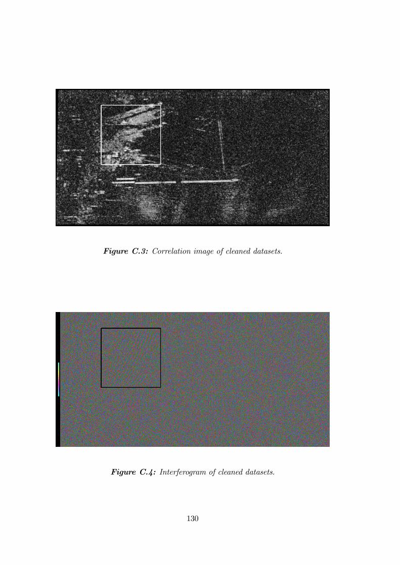
Figure C.3: Correlation image of cleaned datasets.
Figure C.4: Interferogram of cleaned datasets.
130
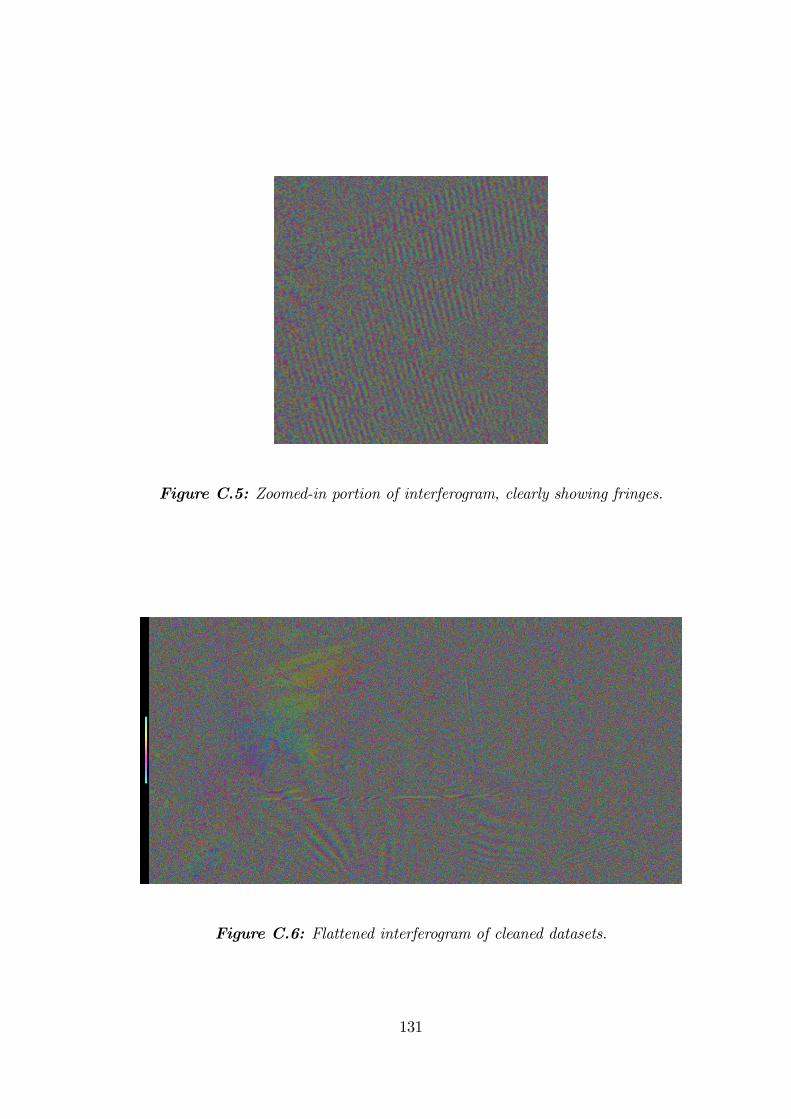
Figure C.5: Zoomed-in portion of interferogram, clearly showing fringes.
Figure C.6: Flattened interferogram of cleaned datasets.
131
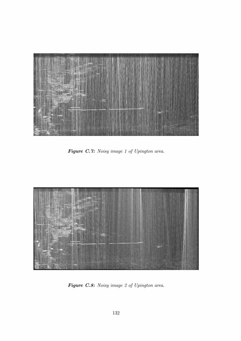
Figure C.7: Noisy image 1 of Upington area.
Figure C.8: Noisy image 2 of Upington area.
132
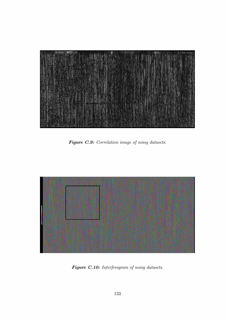
Figure C.9: Correlation image of noisy datasets.
Figure C.10: Interferogram of noisy datasets.
133
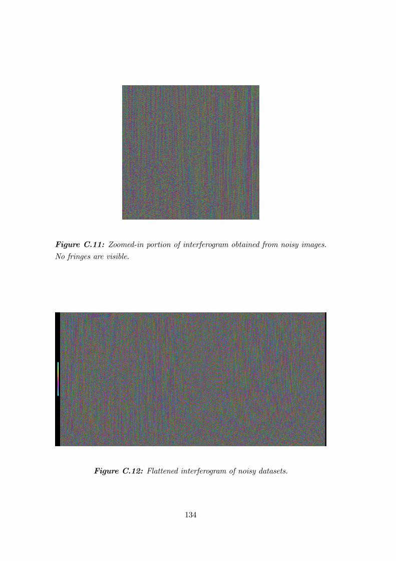
Figure C.11: Zoomed-in portion of interferogram obtained from noisy images.
No fringes are visible.
Figure C.12: Flattened interferogram of noisy datasets.
134
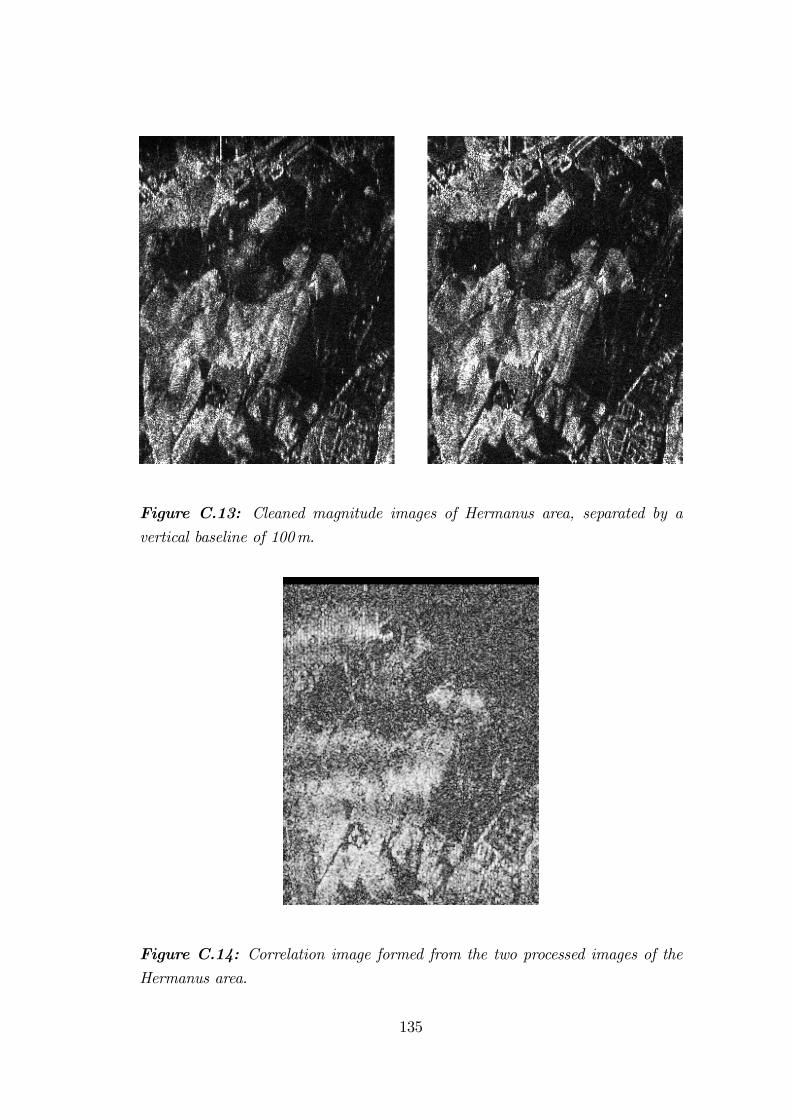
Figure C.13: Cleaned magnitude images of Hermanus area, separated by avertical baseline of 100m.
Figure C.14: Correlation image formed from the two processed images of the
Hermanus area.
135
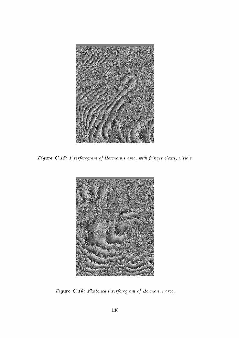
Figure C.15: Interferogram of Hermanus area, with fringes clearly visible.
Figure C.16: Flattened interferogram of Hermanus area.
136
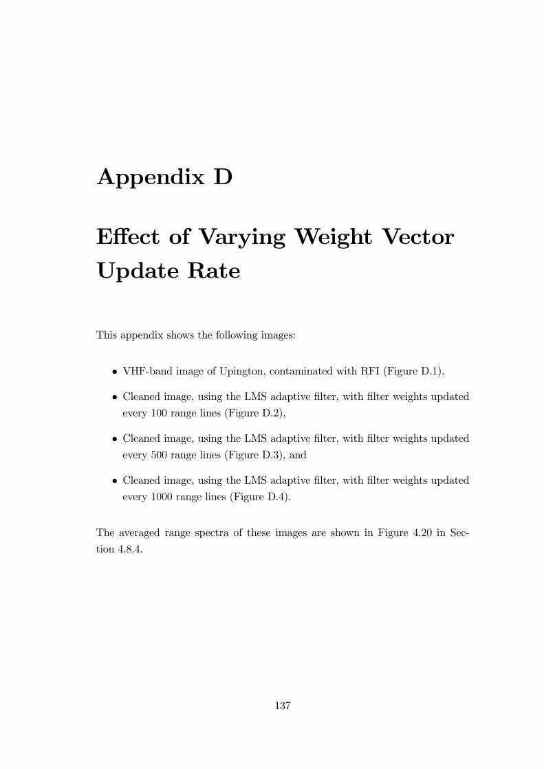
Appendix D
Effect of Varying Weight VectorUpdate Rate
This appendix shows the following images:
• VHF-band image of Upington, contaminated with RFI (Figure D.1),
• Cleaned image, using the LMS adaptive filter, with filter weights updatedevery 100 range lines (Figure D.2),
• Cleaned image, using the LMS adaptive filter, with filter weights updatedevery 500 range lines (Figure D.3), and
• Cleaned image, using the LMS adaptive filter, with filter weights updatedevery 1000 range lines (Figure D.4).
The averaged range spectra of these images are shown in Figure 4.20 in Sec-
tion 4.8.4.
137

Figure D.1: VHF-band image with RFI.
Figure D.2: Cleaned image with weights updated every 100 range lines.
138
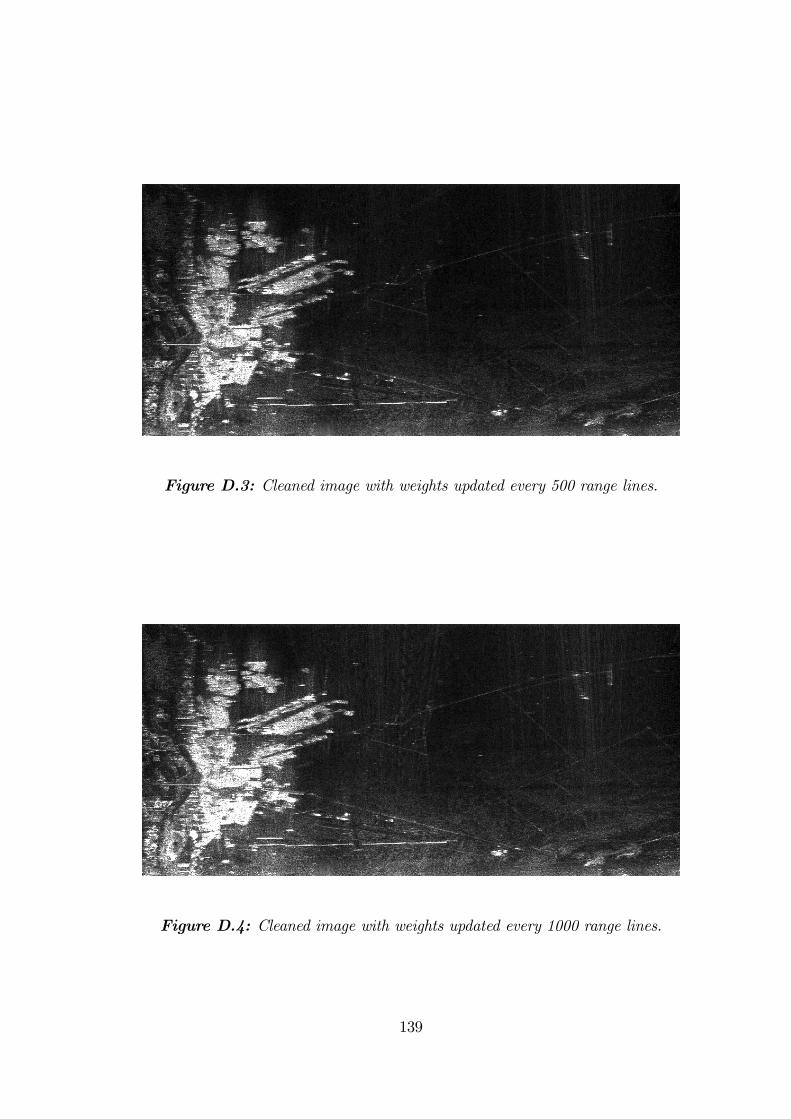
Figure D.3: Cleaned image with weights updated every 500 range lines.
Figure D.4: Cleaned image with weights updated every 1000 range lines.
139

140

Appendix E
Sidelobe Reduction TransferFunction
This appendix shows the derivations of the sidelobe reduction transfer functions
mentioned in Section 4.9. Although all of the signals and transfer functions
mentioned in this appendix are functions of ω, the (ω) symbol has been omitted
in Equations E.1, E.3 and E.5 for reasons of neatness and readability. The
following variables apply in this appendix:
• D (ω) is the RFI contaminated signal;
• E(ω) is the cleaned output of the sidelobe reduction filter;
• H (ω) is the equivalent transfer function of the cleaning filter;
• H1st (ω), H2nd (ω) and H3rd (ω) are the derived transfer functions of thefirst-, second- and third-order sidelobe reduction filters respectively;
• A, B and C are internal signals in the transfer function diagrams.
E.1 First-Order Sidelobe Reduction
Figure E.1 shows the block diagram of the first-order sidelobe reduction transfer
function. Signal B contains the (negative) sidelobe embedded in RFI (refer to
Figure 4.21 (b)), and it is assumed that this sidelobe is sufficiently small, so that
141

D �( )
�+
-
H �( )�
+
H �( )
+
A
B C�( )E
Figure E.1: First-order sidelobe reduction transfer function.
signal C does not contain any “sidelobes of the sidelobe”, after signal B has
passed through the cleaning filter H (ω).
From Figure E.1,
E = A+ C
= A+BH
= DH + (D −DH) H= D 2H −H2 (E.1)
Therefore the first-order transfer function is given by:
H1st (ω) =E(ω)
D(ω)
= H(ω) [2−H(ω)] (E.2)
�+
-
H �( )�
+
H �( )
+
+
-
�
H �( )
�
++
�( )'E
�( )'A
'B
'C
'D
Figure E.2: Second-order sidelobe reduction transfer function.
142
E.2 Second-Order Sidelobe Reduction
Figure E.2 shows the block diagram of the second-order sidelobe reduction trans-
fer function. With the first-order filter the assumption was made that the side-
lobe contained in signal B was sufficiently small, so that signal C did not contain
any “sidelobes of the sidelobe.” If this assumption is not valid, then instead of
passing signal B through the cleaning filter H (ω), it can be passed through the
first-order sidelobe reduction filter H1st (ω). The dashed box in Figure E.2 is
therefore identical to the first-order transfer function shown in Figure E.1.
From Figure E.2,
E = A + C
= A +B H1st
= A + (D −D H) H1st= A + (D −D H) 2H −H2
= D H + 2D H − 2D H2 −D H2 +D H3
= D H 3− 3H +H2 (E.3)
Therefore the second-order transfer function is given by:
H2nd (ω) =E (ω)
D (ω)
= H (ω) 3− 3H (ω) +H (ω)2 (E.4)
E.3 Third-Order Sidelobe Reduction
Figure E.3 shows the block diagram of the third-order sidelobe reduction transfer
function. If the result obtained from the second-order transfer function is still
not satisfactory, then the dashed box shown in Figure E.3 may be replaced
with the second-order sidelobe reduction filter H2nd (ω). This procedure may, in
theory, be continued indefinitely. However, as has been noted in Section 4.9, the
interference suppression capability of the filter is compromised by applying this
sidelobe reduction procedure.
143
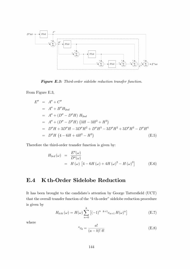
�+
-
H �( )�
+
H �( )
+
+
-
�
H �( )
�
++
+
-
�
H �( )
�
++
�( )''E''C
''B
''A�( )''D
Figure E.3: Third-order sidelobe reduction transfer function.
From Figure E.3,
E = A + C
= A +B H2nd
= A + (D −D H) H2nd
= A + (D −D H) 3H − 3H2 +H3
= D H + 3D H − 3D H2 +D H3 − 3D H2 + 3D H3 −D H4
= D H 4− 6H + 4H2 −H3 (E.5)
Therefore the third-order transfer function is given by:
H3rd (ω) =E (ω)
D (ω)
= H (ω) 4− 6H (ω) + 4H (ω)2 −H (ω)3 (E.6)
E.4 Kth-Order Sidelobe Reduction
It has been brought to the candidate’s attention by George Tattersfield (UCT)
that the overall transfer function of the “k th-order” sidelobe reduction procedure
is given by
Hk th (ω) = H(ω)k
n=0
(−1)n k+1cn+1H(ω)n (E.7)
whereacb =
a!
(a− b)! b! (E.8)
144
Bibliography
Abend, K. and McCorkle, J. (1995). Radio and TV Interference Extraction
for Ultra-Wideband Radar, Algorithms for Synthetic Aperture Radar Im-
agery II (D. A. Giglio, ed.), SPIE, Vol. 2487, Orlando, FL, pp. 119—129.
Axelsson, S. R. J. (1995). Frequency and Azimuthal Variations of Radar Cross
Section and their Influence upon Low-Frequency SAR Imaging, IEEE Trans-
actions on Geoscience and Remote Sensing 33(5): 1258—1265.
Bamler, R. (1992). A Comparison of Range-Doppler and Wavenumber Domain
SAR Focusing Algorithms, IEEE Transactions on Geoscience and Remote
Sensing 30(4): 706—713.
Berlin, G. L., Tarabzouni, M. A., Al-Naser, A. H., Sheikho, K. M. and Larson,
R. W. (1986). SIR-B Subsurface Imaging of a Sand-Buried Landscape:
Al Labbah Plateau, Saudi Arabia, IEEE Transactions on Geoscience and
Remote Sensing 24(4): 595—602.
Braunstein, M., Ralston, J. and Sparrow, D. (1994). Signal Processing Ap-
proaches to Radio Frequency Interference (RFI) Suppression, Algorithms
for Synthetic Aperture Radar Imagery (D. A. Giglio, ed.), SPIE, Vol. 2230,
Orlando, FL, pp. 190—208.
Buckreuss, S. (1997). Development of an Interference Filter for P-Band SAR
Data, Third International Airborne Remote Sensing Conference and Exhi-
bition, Vol. II, Copenhagen, Denmark, pp. 116—121.
Buckreuss, S. (1998). Filtering Interferences from P-Band SAR Data, Proc. Eu-
ropean Conference on Synthetic Aperture Radar, EUSAR’98, VDE-Verlag
GMBH, Berlin and Offenbach, Friedrichshafen, Germany, pp. 279—282.
145

Cafforio, C., Prati, C. and Rocca, E. (1991). SAR Data Focusing Using Seis-
mic Migration Techniques, IEEE Transactions on Aerospace and Electronic
Systems 27(2): 194—207.
Carrara, W. G., Goodman, R. S. and Majewski, R. M. (1995a). Spotlight Syn-
thetic Aperture Radar Signal Processing Algorithms, Artech House, Nor-
wood, MA.
Carrara, W., Tummala, S. and Goodman, R. (1995b). Motion Compensation
Algorithm for Widebeam Stripmap SAR, Algorithms for Synthetic Aperture
Radar Imagery II (D. A. Giglio, ed.), SPIE, Vol. 2487, Orlando, FL, pp. 13—
23.
Cazzaniga, G. and Guarnieri, A. M. (1996). Removing RF Interferences from
P-Band Airplane SAR Data, Proc. IEEE Geosci. Remote Sensing Symp.,
IGARSS’96, Vol. 3, Lincoln, Nebraska, pp. 1845—1847.
Chen, X. (1988). Adaptive Linear-Phase Complex Filtering Algorithms, IEE
Proceedings-F, Vol. 135, pp. 481—486.
Clarke, R. H. and Brown, J. (1980). Diffraction Theory and Antennas, Ellis
Horwood Limited, Chichester.
Crespo, J. C. (1996). The Extended Chirp Scaling Processor for the Experimen-
tal SAR System of DLR, E-SAR, Proc. European Conference on Synthetic
Aperture Radar, EUSAR’96, VDE-Verlag GMBH, Berlin and Offenbach,
Königswinter, Germany, pp. 353—356.
Cumming, I., Wong, F. and Raney, K. (1992). A SAR Processing Algorithm with
No Interpolation, Proc. IEEE Geosci. Remote Sensing Symp., IGARSS’92,
Clear Lake, TX, pp. 376—379.
Curlander, J. C. and McDonough, R. N. (1991). Synthetic Aperture Radar Sys-
tems and Signal Processing, John Wiley and Sons, New York.
Currie, N. C. and Brown, C. E. (1987). Principles and Applications of Millimeter-
Wave Radar, Artech House, Norwood, MA.
Davidson, G. W., Wong, F. and Cumming, I. (1996). The Effect of Pulse Phase
Errors on the Chirp Scaling SAR Processing Algorithm, IEEE Transactions
on Geoscience and Remote Sensing 34(2): 471—478.
146
DPT (1996). Project SABRE (South African Band Re-planning Exercise) - Band
Plan for the Frequencies 20 MHz to 3 GHz, Technical report, Department
of Posts and Telecommunications.
Drinkwater, M. R., Kwok, R. and Rignot, E. (1990). Synthetic Aperture
Radar Polarimetry of Sea Ice, Proc. IEEE Geosci. Remote Sensing Symp.,
IGARSS’90, Washington D.C., USA, pp. 1525—1528.
Elachi, C. (1988). Spaceborne Radar Remote Sensing: Applications and Tech-
niques, IEEE Press, New York.
Elachi, C., Roth, L. E. and Schaber, G. G. (1984). Spaceborne Radar Subsur-
face Imaging in Hyperarid Regions, IEEE Transactions on Geoscience and
Remote Sensing 22(4): 383—387.
Ferrell, B. H. (1995). Interference Suppression in UHF Synthetic-Aperture Radar,
Algorithms for Synthetic Aperture Radar Imagery II (D. A. Giglio, ed.),
SPIE, Vol. 2487, Orlando, FL, pp. 96—106.
Fitch, J. P. (1988). Synthetic Aperture Radar, Springer-Verlag, New York.
Franceschetti, G. and Schirinzi, G. (1990). A SAR Processor Based on Two-
Dimensional FFT Codes, IEEE Transactions on Aerospace and Electronic
Systems 26(2): 356—365.
Gill, G. S. (1995). Step FrequencyWaveformDesign and Processing for Detection
of Moving Targets in Clutter, Proceedings of the IEEE 1995 International
Radar Conference, RADAR’95, Alexandria, Virginia, pp. 573—578.
Glover, J. R. Jr. (1977). Adaptive Noise Cancelling Applied to Sinusoidal In-
terferences, IEEE Transactions on Acoustics, Speech, and Signal Processing
ASSP-25(6): 484—491.
Golden, A. Jr., Werness, S. A., Stuff, M., DeGraaf, S. and Sullivan, R. (1995).
Radio Frequency Interference Removal in a VHF/UHF Deramp SAR, Algo-
rithms for Synthetic Aperture Radar Imagery II (D. A. Giglio, ed.), SPIE,
Vol. 2487, Orlando, FL, pp. 84—95.
Goriachkin, O. V. and Klowsky, D. D. (1997). New Method for Wideband
Low Frequency SAR Data Processing, Third International Airborne Re-
mote Sensing Conference and Exhibition, Vol. II, Copenhagen, Denmark,
pp. 147—154.
147
Goris, M., Joseph, A., Hampson, G. and Smits, F. (1999). Adaptive Beamforming
System for Radio-Frequency Interference Rejection, IEE Proceedings-Radar,
Sonar Navig. 146(2): 73—77.
Griffiths, L. J. (1975). Rapid Measurement of Digital Instantaneous Frequency,
IEEE Transactions on Acoustics, Speech, and Signal Processing ASSP-23(2): 207—222.
Gustavsson, A., Flood, B., Frölind, P.-O., Hellsten, H., Jonsson, T., Larsson,
B., Stenström, G. and Ulander, L. M. H. (1998a). Design and Verification
of a New Airborne 20—90 MHz SAR Sensor, Proc. European Conference
on Synthetic Aperture Radar, EUSAR’98, VDE-Verlag GMBH, Berlin and
Offenbach, Friedrichshafen, Germany, pp. 21—25.
Gustavsson, A., Frölind, P.-O., Hellsten, H., Jonsson, T., Larsson, B. and Sten-
ström, G. (1993). The Airborne VHF SAR System CARABAS, Proc. IEEE
Geosci. Remote Sensing Symp., IGARSS’93, Vol. 2, Tokyo, Japan, pp. 558—
562.
Gustavsson, A., Ulander, L. M. H., Flood, B., Frölind, P.-O., Hellsten, H., Jons-
son, T., Larsson, B. and Stenström, G. (1998b). Development and Operation
of an Airborne VHF SAR System - Lessons Learned, Proc. IEEE Geosci.
Remote Sensing Symp., IGARSS’98.
Harris, F. J. (1978). On the Use of Windows for Harmonic Analysis with the
Discrete Fourier Transform, Proceedings of the IEEE, Vol. 66, pp. 51—83.
Haykin, S. S. (1991). Adaptive Filter Theory, 2nd edn, Prentice-Hall, Englewood
Cliffs, NJ.
Horrell, J. M. (1999). Range-Doppler Synthetic Aperture Radar Processing at
VHF Frequencies, PhD thesis, University of Cape Town.
Hovanessian, S. A. (1984). Radar System Design and Analysis, Artech House,
Norwood, MA.
Hovland, H. A., Johannessen, J. A. and Digranes, G. (1994). Slick Detection
in SAR Images, Proc. IEEE Geosci. Remote Sensing Symp., IGARSS’94,
Pasadena, USA, pp. 2038—2040.
148
Huang, Y., Ma, Z. and Mao, S. (1996). Stepped-frequency SAR System Design
and Signal Processing, Proc. European Conference on Synthetic Aperture
Radar, EUSAR’96, VDE-Verlag GMBH, Berlin and Offenbach, Königswin-
ter, Germany, pp. 565—568.
Hughes, W., Gault, K. and Princz, G. J. (1996). A Comparison of the Range-
Doppler and Chirp Scaling Algorithms with reference to RADARSAT, Proc.
IEEE Geosci. Remote Sensing Symp., IGARSS’96, Vol. 2, Lincoln, Ne-
braska, pp. 1221—1223.
Inggs, M. R. (1996). The SASAR VHF Sensor, Proc. European Conference on
Synthetic Aperture Radar, EUSAR’96, VDE-Verlag GMBH, Berlin and Of-
fenbach, Königswinter, Germany, pp. 317—320.
Inggs, M. R. and Lord, R. T. (1996). SRP Phase VI Status Report, Technical
report, University of Cape Town, Radar Remote Sensing Group, Cape Town.
Inggs, M. R., Hurwitz, J. and Langman, A. (1993). Synthetic Range Profile Mea-
surements of Aircraft, IEEE Proceedings of the 1993 South African Com-
munications and Signal Processing Symposium, COMSIG’93, pp. 204—209.
Inggs, M. R., Knight, A. and Smit, P. (1992a). Synthetic Range Profile Measure-
ments with a Pulse Compression Radar, IEEE Proceedings of the 1992 South
African Communications and Signal Processing Symposium, COMSIG’92,
Cape Town, South Africa, pp. 7—10.
Inggs, M. R., van Zyl, M. W. and Knight, A. (1992b). A Simulation of Synthetic
Range Profile Radar, IEEE Proceedings of the 1992 South African Com-
munications and Signal Processing Symposium, COMSIG’92, Cape Town,
South Africa, pp. 1—6.
Kingsley, S. and Quegan, S. (1999). Understanding Radar Systems, SciTech
Publishing, Mendham.
Kirk, J. C. (1975). A Discussion of Digital Processing in Synthetic Aperture
Radar, IEEE Transactions on Aerospace and Electronic Systems 11(3): 326—337.
Koutsoudis, T. and Lovas, L. (1995). RF Interference Suppression in Ultra Wide-
band Radar Receivers, Algorithms for Synthetic Aperture Radar Imagery II
(D. A. Giglio, ed.), SPIE, Vol. 2487, Orlando, FL, pp. 107—118.
149

Larsson, B., Frölind, P.-O., Gustavsson, A., Hellsten, H., Jonsson, T., Stenström,
G. and Ulander, L. M. H. (1997). Some Results from the New CARABAS II
VHF SAR System, Third International Airborne Remote Sensing Confer-
ence and Exhibition, Vol. I, Copenhagen, Denmark, pp. 25—32.
Le, C. T. C., Hensley, S. and Chapin, E. (1997). Adaptive Filtering of RFI
in Wideband SAR Signals, 7th Annual JPL AirSAR Workshop, Pasadena,
California.
Lengenfelder, R. (1998a). NCTRPhase VIII: Aircraft Data Capture and Analysis
Report, Technical report, University of Cape Town, Radar Remote Sensing
Group, Cape Town.
Lengenfelder, R. (1998b). The Design and Implementation of a Radar Simu-
lator, Technical report, MSc thesis, University of Cape Town, Faculty of
Engineering, Cape Town.
Li, J. and Stoica, P. (1995). Adaptive Filtering Approach to Spectral Estimation
and SAR Imaging, Algorithms for Synthetic Aperture Radar Imagery II
(D. A. Giglio, ed.), SPIE, Vol. 2487, Orlando, FL, pp. 153—164.
Lord, R. T. and Inggs, M. R. (1996). High Resolution VHF SAR Processing Us-
ing Synthetic Range Profiling, Proc. IEEE Geosci. Remote Sensing Symp.,
IGARSS’96, Vol. 1, Lincoln, Nebraska, pp. 454—456.
Lord, R. T. and Inggs, M. R. (1997a). High Range Resolution Radar Using Nar-
rowband Linear Chirps Offset in Frequency, IEEE Proc. of the South African
Symp. on Communications and Signal Processing, COMSIG’97, Graham-
stown, South Africa, pp. 9—12.
Lord, R. T. and Inggs, M. R. (1997b). High Resolution SAR Processing
Using Stepped-Frequencies, Proc. IEEE Geosci. Remote Sensing Symp.,
IGARSS’97, Vol. 1, Singapore, pp. 490—492.
Lord, R. T. and Inggs, M. R. (1998). Approaches to RF Interference Suppression
for VHF/UHF Synthetic Aperture Radar, IEEE Proc. of the South African
Symp. on Communications and Signal Processing, COMSIG’98, Cape Town,
South Africa, pp. 95—100.
Lord, R. T. and Inggs, M. R. (1999a). Efficient RFI Suppression in SAR
Using a LMS Adaptive Filter with Sidelobe Suppression Integrated with
150

the Range-Doppler Algorithm, Proc. IEEE Geosci. Remote Sensing Symp.,
IGARSS’99, Vol. 1, Hamburg, Germany.
Lord, R. T. and Inggs, M. R. (1999b). Efficient RFI Suppression in SAR Using
LMSAdaptive Filter Integrated with Range/Doppler Algorithm, Electronics
Letters 35(8): 629—630.
Lord, R. T. and Inggs, M. R. (2000). Measurements and Characteristics of RFI
for a Low-Bandwidth VHF SAR System, Proc. European Conference on
Synthetic Aperture Radar, EUSAR 2000, VDE Verlag, Munich, Germany,
pp. 845—848.
Lynne, G. J. and Taylor, G. R. (1986). Geological Assessment of SIR-B Imagery
of the Amadeus Basin, N.T., Australia, IEEE Transactions on Geoscience
and Remote Sensing 24(4): 575—581.
Madhukar, C. and Hounam, D. (1998). Feasibility of a Spaceborne P-Band
SAR for Land Surface Imaging, Proc. European Conference on Synthetic
Aperture Radar, EUSAR’98, VDE-Verlag GMBH, Berlin and Offenbach,
Friedrichshafen, Germany, pp. 395—398.
Marple, S. L. Jr. (1987). Digital Spectral Analysis, Prentice-Hall, Englewood
Cliffs, NJ.
Miller, T., McCorkle, J. and Potter, L. (1995). Near-Least-Squares Radio Fre-
quency Interference Suppression, Algorithms for Synthetic Aperture Radar
Imagery II (D. A. Giglio, ed.), SPIE, Vol. 2487, Orlando, FL, pp. 72—83.
Milstein, L. B. (1988). Interference Rejection Techniques in Spread Spectrum
Communications, Proceedings of the IEEE, Vol. 76, pp. 657—671.
Mittermayer, J., Scheiber, R. and Moreira, A. (1996). The Extended Chirp Scal-
ing Algorithm for ScanSAR Data Processing, Proc. European Conference
on Synthetic Aperture Radar, EUSAR’96, VDE-Verlag GMBH, Berlin and
Offenbach, Königswinter, Germany, pp. 517—520.
Mobley, S. and Maier, M. (1996). Synthetic Aperture Radar-Systems Processing
with a Non-Uniform Pulse Repetition Interval, Proc. European Conference
on Synthetic Aperture Radar, EUSAR’96, VDE-Verlag GMBH, Berlin and
Offenbach, Königswinter, Germany, pp. 407—410.
151
Moreira, A., Mittermayer, J. and Scheiber, R. (1996). Extended Chirp Scaling
Algorithm for Air- and Spaceborne SAR Data Processing in Stripmap and
ScanSAR Imaging Modes, IEEE Transactions on Geoscience and Remote
Sensing 34(5): 1123—1136.
Moreira, A., Mittermayer, J. and Scheiber, R. (1998). Processing of SAR and
ScanSAR Imaging Modes using the Extended Chirp Scaling Algorithm,
Proc. European Conference on Synthetic Aperture Radar, EUSAR’98, VDE-
Verlag GMBH, Berlin and Offenbach, Friedrichshafen, Germany, pp. 557—
560.
Munson, D. C. and Visentin, R. L. (1989). A Signal Processing View of
Strip-Mapping Synthetic Aperture Radar, IEEE Transactions on Acoustics,
Speech, and Signal Processing ASSP-37(12): 2131—2147.
Oliver, C. and Quegan, S. (1998). Understanding Synthetic Aperture Radar
Images, Artech House, Boston.
Oppenheim, A. V. (1978). Applications of Digital Signal Processing, Prentice-
Hall, Englewood Cliffs, NJ.
Potsis, A., Reigber, A., Sutor, T. and Papathanassiou, K. P. (1999). A Phase
Preserving Method for RF Interference Suppression in P-Band Synthetic
Aperture Radar Interferometric Data, Proc. IEEE Geosci. Remote Sensing
Symp., IGARSS’99, Vol. 5, Hamburg, Germany.
Prati, C. and Rocca, F. (1992). Range Resolution Enhancement with Multiple
SAR Surveys Combination, Proc. IEEE Geosci. Remote Sensing Symp.,
IGARSS’92, Houston, TX, pp. 1576—1578.
Ralston, J. M. (1998). Ultra-Wide SAR SystemAnalysis, Proc. European Confer-
ence on Synthetic Aperture Radar, EUSAR’98, VDE-Verlag GMBH, Berlin
and Offenbach, Friedrichshafen, Germany, pp. 485—488.
Ralston, J. M., Heagy, J. F. and Sullivan, R. J. (1998). Environmental Noise
Effects on VHF/UHF UWB SAR, Proc. European Conference on Synthetic
Aperture Radar, EUSAR’98, VDE-Verlag GMBH, Berlin and Offenbach,
Friedrichshafen, Germany, pp. 141—144.
Raney, R. K. (1998). Principles and Applications of Imaging Radar - Manual of
Remote Sensing, Vol. 2, 3rd edn, John Wiley and Sons, New York.
152
Raney, R. K., Runge, H., Bamler, R., Cumming, I. G. and Wong, F. H. (1994).
Precision SAR Processing Using Chirp Scaling, IEEE Transactions on Geo-
science and Remote Sensing 32(4): 786—799.
Riegler, R. L. and Compton, R. T. Jr. (1973). An Adaptive Array for Interference
Rejection, Proceedings of the IEEE, Vol. 61, pp. 748—758.
Rihaczek, A. W. (1996). Principles of High-Resolution Radar, Artech House,
Norwood, MA.
Robinson, A. D. and Inggs, M. R. (1994). Correlation Filters Applied to Synthetic
Range Profiles of Aircraft Targets, IEEE Proc. of the South African Symp.
on Communications and Signal Processing, COMSIG’94.
Runge, H. and Bamler, R. (1992). A Novel High Precision SAR Focussing Algo-
rithm Based on Chirp Scaling, Proc. IEEE Geosci. Remote Sensing Symp.,
IGARSS’92, Clear Lake, TX, pp. 372—375.
Sack, M., Ito, M. R. and Cumming, I. G. (1985). Application of Efficient Linear
FM Matched Filtering Algorithms to Synthetic Aperture Radar Processing,
IEE Proceedings, Vol. 132, pp. 45—57.
Schaber, G. G., McCauley, J. F., Breed, C. S. and Olhoeft, G. R. (1986). Shuttle
Imaging Radar: Physical Controls on Signal Penetration and Subsurface
Scattering in the Eastern Sahara, IEEE Transactions on Geoscience and
Remote Sensing 24(4): 603—623.
Schaber, G. G., Olhoeft, G. R. and McCauley, J. F. (1990). The “Radar Rivers”
of the Eastern Sahara: Signal Penetration and Subsurface Scattering Ob-
served by the Shuttle Imaging Radar, Proceedings of 3rd International Con-
ference on GPR, p. 61.
Scheer, J. A. and Kurtz, J. L. (1993). Coherent Radar Performance Estimation,
Artech House, Norwood, MA.
Seger, O., Herberthson, M. and Hellsten, H. (1998). Real Time SAR Processing
of Low Frequency Ultra Wide Band Radar Data, Proc. European Conference
on Synthetic Aperture Radar, EUSAR’98, VDE-Verlag GMBH, Berlin and
Offenbach, Friedrichshafen, Germany, pp. 489—492.
153

Shteinshleiger, V., Dzenkevich, A., Misezhnikov, G. and Mel’nikov, L. (1996). On
the Possibility of Designing a High-Resolution Space-Borne VHF-Band SAR
for Remote Sensing of the Earth, Proc. European Conference on Synthetic
Aperture Radar, EUSAR’96, VDE-Verlag GMBH, Berlin and Offenbach,
Königswinter, Germany, pp. 321—324.
Skolnik, M. I. (1990). Radar Handbook, 2nd edn, McGraw-Hill, New York.
Stimson, G. W. (1983). Introduction to Airborne Radar, Hughes Aircraft Com-
pany, El Segundo, California.
Suess, M., Völker, M., Wilson, J. J. W. and Buck, C. H. (1998). Superresolution:
Range Resolution Improvement by Coherent Combination of Repeat Pass
SAR Images, Proc. European Conference on Synthetic Aperture Radar, EU-
SAR’98, VDE-Verlag GMBH, Berlin and Offenbach, Friedrichshafen, Ger-
many, pp. 565—569.
Taylor, J. D. (ed.) (1995). Introduction to Ultra-Wideband Radar Systems, CRC
Press, Boca Raton, Florida.
Trizna, D. and Sletten, M. (1997). NUWSAR - NRL Ultra Wideband Synthetic
Aperture Radar an Experimental Tool for Remote Sensing Studies, Third
International Airborne Remote Sensing Conference and Exhibition, Vol. II,
Copenhagen, Denmark, pp. 68—73.
Ulander, L. M. H. (1998). Performance of Stepped-Frequency Waveform
for Ultra-Wideband VHF SAR, Proc. European Conference on Synthetic
Aperture Radar, EUSAR’98, VDE-Verlag GMBH, Berlin and Offenbach,
Friedrichshafen, Germany, pp. 323—326.
Ulander, L. M. H. and Frölind, P.-O. (1999). Precision Processing of CARABAS
HF/VHF-band SAR Data, Proc. IEEE Geosci. Remote Sensing Symp.,
IGARSS’99, Vol. 1, Hamburg, Germany.
Ulander, L. M. H. and Hellsten, H. (1997). System Analysis of Ultra-Wideband
VHF SAR, Proceedings of the IEEE 1997 International Radar Conference,
RADAR’97, Edinburgh, UK, pp. 104—108.
Vant, M. R. (1989). Synthetic Aperture Radar Signal Processing, Proceedings of
the 1989 International Conference on Radar.
154
Wahl, T. and Skoelv, A. (1994). ERS-1 SAR Imaging of Ocean Features in the
Vestfjorden Area, Proc. IEEE Geosci. Remote Sensing Symp., IGARSS’94,
Pasadena, USA, pp. 2035—2037.
Walter, F., Fransson, J. E. S. and Frölind, P.-O. (1999). Fully Automatic Geo-
coding of CARABAS-II VHF SAR Images, Proc. IEEE Geosci. Remote
Sensing Symp., IGARSS’99, Vol. 1, Hamburg, Germany.
Wehner, D. R. (1995). High-Resolution Radar, 2nd edn, Artech House, Norwood,
MA.
Widrow, B. and Stearns, S. D. (1985). Adaptive Signal Processing, Prentice-Hall,
Englewood Cliffs, NJ.
Widrow, B., Glover, J. R. Jr., McCool, J. M., Kaunitz, J., Williams, C. S., Hearn,
R. H., Zeidler, J. R., Dong, E. Jr. and Goodlin, R. C. (1975a). Adaptive
Noise Cancelling: Principles and Applications, Proceedings of the IEEE,
Vol. 63, pp. 1692—1716.
Widrow, B., McCool, J. and Ball, M. (1975b). The Complex LMS Algorithm,
Proceedings Letters of the IEEE, pp. 719—720.
Wilkinson, A. J. (1996). Notes on Synthetic Range Profiling, Technical re-
port, University of Cape Town, Department of Electrical Engineering, Cape
Town, April 1996.
Wilkinson, A. J., Lord, R. T. and Inggs, M. R. (1998). Stepped-Frequency
Processing by Reconstruction of Target Reflectivity Spectrum, IEEE Proc.
of the South African Symp. on Communications and Signal Processing,
COMSIG’98, Cape Town, South Africa, pp. 101—104.
Zeidler, J. R., Satorius, E. H., Chabries, D. M. and Wexler, H. T. (1978). Adap-
tive Enhancement of Multiple Sinusoids in Uncorrelated Noise, IEEE Trans-
actions on Acoustics, Speech, and Signal Processing ASSP-26(3): 240—254.
155