
Aspect of classical density functional theory: crystals ...
132
Aspect of classical density functional theory: crystals and interfaces in hard–disk systems and the problem of constructing functionals using machine learning methods Dissertation der Mathematisch-Naturwissenschaftlichen Fakult¨ at der Eberhard Karls Universit¨ at T¨ ubingen zur Erlangung des Grades eines Doktors der Naturwissenschaften (Dr. rer. nat.) vorgelegt von Shang–Chun Lin aus Tainan/ Taiwan T¨ ubingen 2020
Transcript of Aspect of classical density functional theory: crystals ...
Aspect of classical density functional theory:
crystals and interfaces in hard–disk systems
andthe problem of constructing functionals using
machine learning methods
Dissertationder Mathematisch-Naturwissenschaftlichen Fakultat
der Eberhard Karls Universitat Tubingenzur Erlangung des Grades eines
Doktors der Naturwissenschaften(Dr. rer. nat.)
vorgelegt vonShang–Chun Linaus Tainan/ Taiwan
Tubingen2020


Gedruckt mit Genehmigung der Mathematisch-Naturwissenschaftlichen Fakultatder Eberhard Karls Universitat Tubingen.
Tag der mundlichen Qualifikation: 12.02.2021Stellvertretender Dekan: Prof. Dr. Jozsef Fortagh1. Berichterstatter: Prof. Dr. Martin Oettel2. Berichterstatter: Prof. Dr. Roland Roth

List of published work
Most results of this thesis have already been published in academic journals,and the corresponding publications are listed as following.
Phase diagrams and crystal–fluid surface tensions in additive andnonadditive two–dimensional binary hard–disk mixturesShang-Chun Lin and Martin Oettel, Physical Review E 98.1.012608 (2018),DOI: 10.1103/PhysRevE.98.012608
Abstract: Using density functionals from fundamental measuretheory, phase diagrams and crystal–fluid surface tensions in addi-tive and nonadditive (Asakura–Oosawa model) two–dimensionalbinary hard–disk mixtures are determined for the whole rangeof size ratios q=small diameter/large diameter, assuming randomdisorder (lattice points or interstitial occupied by large or smalldisks at random) in the crystal phase. The fluid–crystal transi-tions are first order due to the assumption of a periodic unit cellin the density–functional calculations. Qualitatively, the shapeof the phase diagrams is similar to the case of three–dimensionalhard–sphere mixtures. For the nonadditive case, a broadening ofthe fluid–crystal coexistence region is found for small q, whereasfor large q a vapor–fluid transition intervenes. In the additivecase, we find a sequence of spindle , azeotropic, and eutecticphase diagrams upon lowering q from 1 to 0.6. The transitionfrom azeotropic to eutectic is different from the three–dimensionalcase. Surface tensions in general become smaller (up to a factor 2)upon the addition of a second species and they are rather small.The minimization of the functionals proceeds without restrictionsand optimized graphics card routines are used.
Statement of the author : Motivated by the successful results for one–componenthard–sphere systems, we systematically investigated crystal–fluid interfacesand phase diagrams in binary hard–disk systems.
i

ii
A classical density functional from machine learning and a convo-lutional neural networkShang-Chun Lin and Martin Oettel, SciPost Phys. 6, 025 (2019),DOI: 10.21468/SciPostPhys.6.2.025
Abstract: We use machine learning methods to approximate aclassical density functional. As a study case, we choose the modelproblem of a Lennard Jones fluid in one dimension where thereis no exact solution available and training data sets must be ob-tained from simulations. After separating the excess free energyfunctional into a ”repulsive” and an ”attractive” part, machinelearning finds a functional in weighted density form for the attrac-tive part. The density profile at a hard wall shows good agreementfor thermodynamic conditions beyond the training set conditions.This also holds for the equation of state if it is evaluated near thetraining temperature. We discuss the applicability to problems inhigher dimensions.
Statement of the author : I used a convolutional network to learn the explicitexcess free energy functional. The idea was completely new and I have hadbuilt it from the ground up. Since I was lack of knowledge of machine learn-ing at the time, the functionals are limited to simple polynomial ansatze andthe training process was written purely by Numpy, which is incredibly slowcomparing to the later work. However, the results are better than we ex-pected and thus prove the point that it is possible to approximate unknownfunctionals explicitly by machine learning.
iii
Analytical classical density functionals from an equation learningnetworkShang-Chun Lin, Georg Martius and Martin Oettel, J. Chem. Phys. 152,021102 (2020),DOI: 10.1063/1.5135919
Abstract: We explore the feasibility of using machine learningmethods to obtain an analytic form of the classical free energyfunctional for two model fluids, hard rods and Lennard–Jones,in one dimension . The Equation Learning Network proposedin Ref. [1] is suitably modified to construct free energy densitieswhich are functions of a set of weighted densities and which arebuilt from a small number of basis functions with flexible com-bination rules. This setup considerably enlarges the functionalspace used in the machine learning optimization as compared toprevious work [2] where the functional is limited to a simple poly-nomial form. As a result, we find a good approximation for theexact hard–rod functional and its direct correlation function. Forthe Lennard–Jones fluid, we let the network learn (i) the full ex-cess free energy functional and (ii) the excess free energy func-tional related to interparticle attractions. Both functionals showa good agreement with simulated density profiles for thermody-namic parameters inside and outside the training region.
Statement of the author : With the previous successful work, Martin and Icollaborated with Dr. Georg Martius to extend the feasibility and reliabilityof the network. The functional can have complex representations with simplebasis functions. The training process was written by Tensorflow and Sympy
with GPU (graphics processing unit) accelerated. The results and the speedof the training process are significantly improved comparing to the previouswork. Even though there is still a lot of room to improve, I believe it couldbe the future for approximating unknown functionals.

Abstract
The theoretical studies reported in this thesis are mainly concerned with twotopics in classical density functional theory (DFT). First, we investigate thecrystal–fluid interface and phase transitions in hard–disk systems. Second,we propose a novel machine learning architecture, the Functional EquationLearner, to obtain an explicit free energy functional directly from equilibriumdensity distributions in the presence of different external potentials.
For this purpose, we briefly introduce DFT and Fundamental MeasureTheory (FMT). DFT is an approach for evaluating the free energy based onparticle density distributions, and FMT is a particular instance of DFT forhard spheres in three, two and one dimensions, which gives highly accurate(in two and three dimensions) or exact (in one dimension) descriptions of ho-mogeneous and inhomogeneous systems. For two–dimensional hard spheres(hard disks), we use the free energy functional based on FMT proposed byRoth et al. [3], which has been previously reported to show accurate ther-modynamic properties for a triangular crystalline structure and crystal–fluidcoexistence densities compared to Monte–Carlo simulations.
For one–component hard–disk systems, our result for the surface tensionof a crystal–liquid interface is in good agreement with experiments, and themelting transition is investigated. As has been confirmed in past years, themelting transition for hard disks proceeds via the formation of a “hexatic”phase. In our numerical experiment, the characteristics of a hexatic phase,i.e. dislocations, are found. Furthermore, we model genuine hard–disk mix-tures and mixtures of hard disks with non–additive polymers to obtain phasediagrams and surface tensions. For genuine hard–disk mixtures, the phasediagrams are qualitatively very similar to those of three–dimensional hardspheres, where the sequence of types of phase diagrams spindle→ azeotropic→ eutectic is observed upon lowering the small size ratio from 1 to 0.6. Fornon–additive mixtures, the free energy functional is linearized with respectto the polymer density, which is analogous to a known DFT approach to thethree–dimensional Asakura–Oosawa model. In this case, the typical continu-ous widening of the coexistence gap between fluid and solid is observed upon
v
vi
the addition of the smaller species. For the surface tension, it shows that theaddition of a second component leads in general to a substantial decrease forboth genuine and non–additive hard–disk mixtures.
Furthermore, despite that FMT provides highly accurate free energy func-tionals for hard particles, a FMT like treatment for a non–vanishing inter-action outside the hard core is missing. In general, in such a case, the an-alytical form of the free energy functional is unknown; therefore we adoptthe recently introduced equation learning network [1] and propose the Func-tional Equation Learner (FEQL) for this task. With flexible combinationrules, composite functions from the FEQL are built from a number of ba-sis functions and a set of weighted densities. The training, i.e. tuning theparameters in functions, is automatically done by minimizing the Euclideandistance between predicted and exact/simulated density distributions. As aresult, we find well approximated free energy functionals for the hard–rodfluid (exact functional is known) and the Lennard–Jones fluid (exact func-tional is unknown). In both cases, the density profiles, equation of states,and the direct correlation functions delivered by the learned functionals arein good agreement with exact/simulated results, even outside the trainingregions.

Zusammenfassung
Die theoretischen Studien, uber die in dieser Arbeit berichtet wird, befassensich hauptsachlich mit zwei Themen der klassischen Dichtefunktionaltheorie(DFT). Zunachst untersuchen wir die Kristall-Fluid-Grenzflache und Phasen-ubergange in Harte–Scheiben–Systemen. Zweitens, stellen wir eine neuar-tige maschinelle Lernarchitektur vor, den Functional Equation Learner , umexplizit Funktionale der freien Energie zu erhalten, welche direkt aus Gle-ichgewichtsdichteverteilungen unter dem Einfluss verschiedener externer Po-tentiale berechnet werden.
Zu diesem Zweck stellen wir die DFT und die Fundamental Measure The-ory (FMT) kurz vor. Die DFT ist ein Ansatz zur Berechnung der freienEnergie auf der Grundlage von Partikeldichteverteilungen, und die FMT isteine besondere Auspragung der DFT fur harte Kugelnn in drei, zwei undeiner Dimension(en), die eine hochgenaue (in zwei und drei Dimensionen)oder exakte (in einer Dimension) Beschreibung von homogenen und inhomo-genen Systemen liefert. Fur zweidimensionale harte Kugeln (harte Scheiben)verwenden wir das von Roth et al. [3] vorgeschlagene Funktional der freienEnergie auf der Grundlage der FMT, wovon bereits fruher berichtet wurde,dass es im Vergleich zu Monte–Carlo–Simulationen genaue thermodynamis-che Eigenschaften fur eine dreieckige kristalline Struktur und Kristall–Fluid–Koexistenzdichten vorhersagt.
Fur einkomponentige Harte–Scheiben–Systeme ist unser Ergebnis fur dieOberflachenspannung einer Kristall–Flussigkeits-Grenzflache in guter Uber-einstimmung mit Experimenten, ausserdem wird der Schmelzubergang un-tersucht. Wie in den vergangenen Jahren bestatigt wurde, verlauft derSchmelzubergang bei Harten–Scheiben uber die Bildung einer “hexatischen”Phase. In unserem numerischen Experiment werden die Eigenschaften einerhexatischen Phase, z.B. Dislokationen, gefunden. Daruber hinaus model-lieren wir Harte–Scheiben–Mischungen und Mischungen von Harte–Scheibenmit nicht–additiven Polymeren, um Phasendiagramme und Oberflachenspan-nungen zu erhalten. Fur additive Harte–Scheiben–Mischungen sind die Phasen-diagramme qualitativ sehr ahnlich denen von dreidimensionalen Harte–Kugeln–
vii

viii
Systemen, wobei die Abfolge von Phasendiagrammen des Types spindelformig→ azeotropen → eutektischen beim Absenken des Großenverhaltnisses derkleinen Spezies von 1 auf 0.6 beobachtet wird. Fur nicht–additive Mischun-gen wird das Freie–Energie–Funktional in Bezug auf die Polymerdichte lin-earisiert, was analog zu einem bekannten DFT–Ansatz des drei–dimensionalenAsakura–Oosawa–Modells geschieht. In diesem Fall wird die typische kon-tinuierliche Vergroßerung der Koexistenzlucke zwischen Flussigkeit und Fest-korper bei der Zugabe der kleineren Spezies beobachtet. Fur die Oberflachen-spannung zeigt sich, dass die Zugabe einer zweiten Komponente im All-gemeinen zu einer erheblichen Abnahme sowohl bei additiven als auch beinicht–additiven Harte–Scheiben–Mischungen fuhrt.
Obwohl die FMT hochprazise Funktionale der freien Energie fur harteTeilchen liefert, fehlt eine FMT–ahnliche Methode fur die Wechselwirkungaußerhalb des harten Kerns. Im Allgemeinen ist in einem solchen Fall die an-alytische Form des Freie–Energie–Funktionals unbekannt; daher ubernehmenwir das kurzlich eingefuhrte Gleichungslern–Netzwerk [1] und stellen denFunctional Equation Learner (FEQL) fur diese Aufgabe vor. Mit flexiblenKombinationsregeln werden zusammengesetzte Funktionen aus dem FEQLaus einer Reihe von Basisfunktionen und einem Satz gewichteter Dichtengebildet. Das Training, d.h. die Abstimmung der Parameter in Funktionen,erfolgt automatisch durch Minimierung des euklidischen Abstands zwischenvorhergesagten und exakten/simulierten Dichteverteilungen. Als Ergebnisfinden wir gut approximierte Funktionale der freien Energie fur das Harte–Stabchen–Fluid (das genaue Funktional ist bekannt) und das Lennard-Jones-Fluid (das genaue Funktional ist unbekannt). In beiden Fallen stimmen dieDichteprofile, die Zustandsgleichungen und die direkten Korrelationsfunk-tionen, die von den gelernten Funktionalen geliefert werden, mit den exak-ten/simulierten Ergebnissen uberein, auch außerhalb der Trainingsregionen.

Contents
1 Introduction 1
2 Thermodynamics and statistical physics 52.1 Canonical ensemble . . . . . . . . . . . . . . . . . . . . . . . . 62.2 Grand canonical ensemble . . . . . . . . . . . . . . . . . . . . 72.3 Ideal gas and density distribution functions . . . . . . . . . . . 82.4 Classical density functional theory . . . . . . . . . . . . . . . . 9
3 Approximating the excess free energy 133.1 Density expansion and direct correlation function . . . . . . . 133.2 Ornstein–Zernike relation . . . . . . . . . . . . . . . . . . . . . 143.3 Fundamental measure theory . . . . . . . . . . . . . . . . . . . 16
3.3.1 Three–dimensional hard spheres . . . . . . . . . . . . . 163.3.2 Two–dimensional hard disks . . . . . . . . . . . . . . . 223.3.3 One–dimensional hard rods . . . . . . . . . . . . . . . 23
4 One–component hard disks 254.1 Bulk phase and coexistence . . . . . . . . . . . . . . . . . . . 26
4.1.1 Bulk phase . . . . . . . . . . . . . . . . . . . . . . . . 264.1.2 Coexistence . . . . . . . . . . . . . . . . . . . . . . . . 27
4.2 Planar interface and surface tension . . . . . . . . . . . . . . . 294.2.1 Planar surface tension . . . . . . . . . . . . . . . . . . 31
4.3 Phase transition and crystal nuclei . . . . . . . . . . . . . . . 334.4 Hexatic phase . . . . . . . . . . . . . . . . . . . . . . . . . . . 354.5 Conclusion . . . . . . . . . . . . . . . . . . . . . . . . . . . . . 39
5 Hard–disk binary mixtures 415.1 Free energy functional . . . . . . . . . . . . . . . . . . . . . . 435.2 Crystal density profiles . . . . . . . . . . . . . . . . . . . . . . 445.3 Phase diagrams . . . . . . . . . . . . . . . . . . . . . . . . . . 46
5.3.1 Small size ratios q . . . . . . . . . . . . . . . . . . . . . 46
ix
x CONTENTS
5.3.2 Intermediate size ratios q . . . . . . . . . . . . . . . . . 48
5.3.3 Size ratios q close to 1 . . . . . . . . . . . . . . . . . . 48
5.4 Interface density profiles . . . . . . . . . . . . . . . . . . . . . 50
5.5 Crystal–fluid surface tensions . . . . . . . . . . . . . . . . . . 53
5.5.1 Size ratio q ≤ 0.6 . . . . . . . . . . . . . . . . . . . . . 53
5.5.2 Size ratio q ≥ 0.75: HD mixtures . . . . . . . . . . . . 54
5.6 Liquid–vapor surface tension . . . . . . . . . . . . . . . . . . . 55
5.7 Summary and conclusion . . . . . . . . . . . . . . . . . . . . . 56
6 Machine learning functional 59
6.1 Basic ideas and improved mean–field functionals . . . . . . . . 60
6.2 Result and conclusion . . . . . . . . . . . . . . . . . . . . . . . 62
7 Functional equation learner 65
7.1 Physical constraints . . . . . . . . . . . . . . . . . . . . . . . . 68
7.2 Network training . . . . . . . . . . . . . . . . . . . . . . . . . 68
7.3 Results . . . . . . . . . . . . . . . . . . . . . . . . . . . . . . . 69
7.3.1 Hard rods . . . . . . . . . . . . . . . . . . . . . . . . . 69
7.3.2 Lennard–Jones . . . . . . . . . . . . . . . . . . . . . . 72
7.3.3 Explicit functional and convolution kernels . . . . . . . 75
7.3.4 Consistency of µ . . . . . . . . . . . . . . . . . . . . . 77
7.3.5 Direct correlation function . . . . . . . . . . . . . . . . 79
7.3.6 Learning the exact HR functional . . . . . . . . . . . . 80
7.4 Conclusion . . . . . . . . . . . . . . . . . . . . . . . . . . . . . 82
Appendices 85
A Convolution and Fourier transformation 87
A.1 Convolution . . . . . . . . . . . . . . . . . . . . . . . . . . . . 87
A.2 Fourier transformation in FMT . . . . . . . . . . . . . . . . . 88
A.2.1 3D . . . . . . . . . . . . . . . . . . . . . . . . . . . . . 88
A.2.2 2D . . . . . . . . . . . . . . . . . . . . . . . . . . . . . 89
A.2.3 1D . . . . . . . . . . . . . . . . . . . . . . . . . . . . . 91
A.3 Numerics . . . . . . . . . . . . . . . . . . . . . . . . . . . . . 91
B Free energy minimization 93
B.1 Picard method . . . . . . . . . . . . . . . . . . . . . . . . . . 94
B.2 Direct inversion in iterative subspace . . . . . . . . . . . . . . 94
B.3 Dynamic density functional theory . . . . . . . . . . . . . . . 95
B.4 Convergence . . . . . . . . . . . . . . . . . . . . . . . . . . . . 97

CONTENTS xi
C Direct correlation function by FMT 99C.1 Homogeneous cases . . . . . . . . . . . . . . . . . . . . . . . . 100C.2 Inhomogeneous . . . . . . . . . . . . . . . . . . . . . . . . . . 101
C.2.1 Crystal . . . . . . . . . . . . . . . . . . . . . . . . . . . 102C.3 Conclusion . . . . . . . . . . . . . . . . . . . . . . . . . . . . . 104

Chapter 1
Introduction
God made the bulk; the surface was invented by the devil.– Wolfgang Pauli
If we would like to make something that runs rapidly over the ground, thenwe could watch a cheetah running, and we could try to make a machine that
runs like a cheetah. But, it’s easier to make a machine with wheels.– Richard Feynman
Surfaces or interfaces are the locations for many phenomena between thematerial and its environment, where all physical and chemical interactionsand exchanges take place. To observe interfaces, colloidal systems serve asimportant tools and model systems. The length scale of colloidal systems ismicrometers; thus, single–particle resolution can be achieved, for example,by confocal microscopy. More importantly, the pairwise interaction betweenthe particles makes it possible to study the system by methods of classicalstatistical mechanics, e.g. Monte–Carlo simulation or density functional the-ory (DFT). As a result, the one–to–one comparison between experiments andclassical statistical mechanics is possible.
In colloidal systems, the interaction is usually composed of a the short–ranged harsh repulsion and long–ranged smooth attraction. The short–rangerepulsion plays a crucial role as it determines the main structure of the liquidand crystal phase. Therefore, hard spheres (HS), where the harsh short–rangerepulsion forbids overlaps, serves as an important reference system. As thereis no attraction between HS particles, the crystal–fluid transition is purelyinduced by entropy.
For a theoretical understanding of HS, density functional theory (DFT)is a very important tool which gives a description of both microsopic andmacrosopic (bulk) properties in equilibrium. The challenge of DFT is to
1
2 CHAPTER 1. INTRODUCTION
approximate the free energy as precisely as possible. In 1989, Rosenfeld in-troduced fundamental measure theory (FMT) as a DFT treatment for HSmixtures in three, two and one dimension [4, 5]. During the next two decades,the FMT has been further developed and gives almost exact results in com-parison with simulations [3, 6, 7, 8].
Unfortunately, such success is missing with respect to the long–rangedsmooth attraction. In DFT, the attractions are usually treated as a per-turbation; however, for low enough temperatures, attractions can dominateover repulsions and thus perturbative treatments, such as the mean–fieldapproximation, are able to deliver a qualitative description but usually arequantitatively inaccurate, or require more effort [9]. Recently, with the greatimprovement of computational hardware, machine learning methods havebeen developed and used to give computers the ability to analyze patternswithin a given data set without programming explicitly. For DFT, this im-plies the possibility to learn the free energy functionals by inputs, for in-stance, one–body density distributions and external potentials, without theexplicit knowledge of many–body correlations.
In this thesis, after a brief introduction of thermodynamics and statisticalphysics in Chapter 2, the DFT approaches to the excess free energy relevantto this thesis are introduced in Chapter 3. The main results are split intotwo parts: fluid–crystal transitions and interfaces of two–dimensional hard–disk mixtures (Chapter 4 and 5), and machine learning functionals of one–dimensional fluids (Chapter 6 and 7).
Two–dimensional hard–disk mixtures
In two–dimensional (2D) systems, the fluid–crystal transition of hard–diskmixtures has been of fundamental interest over the past years. Only recently,it has been established in the one–component system by simulations [10] andexperiments [11] that the transition happens via a first–order transition fromthe fluid to the hexatic phase and a continuous transition from the hexaticto the crystal phase. Although the crystal phase is not strictly periodic (itdoes not have infinitely long–ranged positional order), in simulations andexperiments it has practically the appearance of a conventional, periodiccrystal.
By using the density functional from fundamental measure theory pro-posed in Ref. [3], which gives a very accurate description of fluid structure inone– and two–component systems[12], the phase diagrams and crystal–fluidsurface tensions in two–dimensional hard–disk binary mixtures are deter-mined. The minimization of the functionals proceeds without restrictions.
For one–component hard disks, the thermodynamic properties at coex-
3
istence and crystal–fluid surface tensions are close to simulations [10] andexperiments [11]. Also, the anisotropy of surface tensions are determinedwhich, however, is about one magnitude smaller than in experiments [11].Furthermore, we investigate the hexatic phase by measuring the pair cor-relation function in large systems, here, the results are not conclusive withregard to a connect DFT description of the hexatic phase.
For mixtures, we consider a simple binary mixture of large (l) and small(s) disks, with diameter σl and σs, respectively, and q = σs
σldenoting the size
ratio. In the case of an additive system (denoted as HD mixture), one maydefine an interaction diameter dij = σi/2 + σj/2 with i, j = l, s. The pairpotential Φij(r) between two particles with center-center distance r is ∞ forr < dij and 0 for r > dij. In addition, we consider a non additive mixturein which the interaction between two small disks is zero, i.e. they behave asan ideal gas and the other interactions (large–large and large–small) remainunchanged. This mixture is the 2D variant [13] of the well–known Asakura–Oosawa (AO) model [14, 15]. For the nonadditive case, a broadening of thefluid–crystal coexistence region is found for small q whereas for higher q avapor–fluid transition intervenes. In the additive case, we find a sequence ofspindle type, azeotropic and eutectic phase diagrams upon lowering q from 1to 0.6. The transition from azeotropic to eutectic is different from the three–dimensional case. Surface tensions in general are rather small and becomesmaller (up to a factor 2) upon addition of a second species.
Machine learning functionals
The art of DFT is the construction of free energy functionals. The densitydistributions are computed by self–consistent equations involving functionalderivatives of these free energy functionals, and these equations are solv-able with much less numerical effort than obtaining density distributions insimulations. Furthermore, all equilibrium and even some non–equilibriumproperties are based on the free energy functionals. Despite the great prin-ciple power of the approach, the exact free energy functionals are not knownin general, therefore considerable effort has gone into the theoretical develop-ment of functionals. As mentioned, the functionals derived from FMT havea high degree of accuracy for hard particles, but for the interactions outsidethe hard core, a qualitatively new and successful ansatz is missing.
In recent years, some effort has gone into approximating (“learning”)functionals by machine learning (ML) techniques. In quantum DFT, e.g., in-terpolating functionals generated by kernel ridge regression have been testedfor model 1D systems [16, 17] and also have been extended to 3D systems [18].Numerically interpolated functionals do not contain sufficient information
4 CHAPTER 1. INTRODUCTION
about functional gradients, therefore both the energy–density map and theexternal potential–density maps had to be learned by interpolation [17]. Forthe 1D Hubbard model, a convolutional network functional has been learnedwhose numerical functional derivative appears to be more robust [19]. How-ever, these approaches hide the energy functional inside an “ML black box”which does not permit much insight from a theory perspective. For theclassical case, a 1D LJ–like fluid was studied by us with a convolutional net-work [2], utilizing an established approach from liquid state theory of splittingthe excess free energy functional into a “repulsion” part and an “attraction”part F att [2]. The convolutional network naturally leads to an approxima-tion of F att in terms of weighted densities ni, which are the essential buildingblocks in modern classical DFT; however, the free energy density fex
att(ni) as afunction of ni had to be prescribed as simple polynomials. An interpretableresults obtained in [2] was the accurate splitting of the interaction potentialin the Weeks–Chandler–Andersen (WCA) spirit [20].
In this context, the question naturally arises whether ML techniques canbe used to learn analytic forms of (free) energy functionals instead of “blackboxes” or presumed forms. This question is important also in a more generalcontext: can ML algorithms contribute to theory building in physics? Inthe ML community, efforts in that direction have utilized genetic algorithmsto search a space of simple basis function with multiplication and additionrules [21]. More recent work by us proposes an equation learning network em-ploying gradient-based optimization with simple basis functions and divisionbesides multiplication/addition as combination rules [1, 22]. An empiricalprinciple for the “right” formula (choose the simplest one that still predictswell, i.e. Occam’s razor) can be built into the loss function. This princi-ple was also successful in the history of physics in finding analytical modelswith high predictive power even outside the training/observed regime. Forthe DFT problem, the extrapolation power to other external potentials is animportant aspect, as well as the analytic differentiability of the free energyfunctional since structural information about the fluid (pair correlations) isobtained via the direct correlation function (two functional derivatives of theexcess free energy functional).
These aspects are explored for the model cases of a hard–rod (HR) and aLennard–Jones (LJ) fluid in 1D. As a result, we find a good approximationfor the exact hard–rod functional and its direct correlation function. For theLennard–Jones fluid, we let the network learn (i) the full excess free energyfunctional and (ii) the excess free energy functional related to interparticleattractions. Both functionals show a good agreement with simulated densityprofiles for thermodynamic parameters inside and outside the training region.
Chapter 2
Thermodynamics andstatistical physics
In this chapter, only essential ingredients are introduced. We refer to thebook Theory of simple liquids [23] for readers who have a deeper interest.
A D–dimensional system with N particles has 2 × D × N coordinatesin phase space, i.e. the positions rN = (r1, r2...rN) and momenta pN =(p1,p2...pN) with ri and pi the location and momentum of particle i. LetΓ = (r1...rN ,p1, ...,pN ;N) denote a point in phase space; more precisely, Γis called ‘microstate’ or ‘configuration’ of the system. The average value 〈O〉of an observable O(Γ) is defined by
〈O〉 =∑
Γ
O(Γ)f(Γ) ≡ trclO(Γ)f(Γ) (2.1)
with f(Γ) the probability in phase space and trcl the classical trace (thesummation over all possible configurations), as defined in Eqs. (2.9) and(2.14) below for different ensembles.
In equilibrium, the explicit expression for the phase space probability feq
can be obtained from the Gibbs principle of maximum (Shannon) entropy S,which is defined as
S = max (−kB 〈ln (feq)〉) = −kBtrclfeq ln(feq). (2.2)
The HamiltonianH of a system is a sum of the kinetic energy T , interparticlepotential energy U , and the external potential V ext; i.e.,
H(rN ,pN) = T (pN) + U(rN) + V ext(rN), (2.3)
where
T (pN) =N∑
i=1
p2i
2mi
, (2.4)
5

6 CHAPTER 2. THERMODYNAMICS AND STATISTICAL PHYSICS
U(rN) =∑
i<j
ψ(ri, rj), (2.5)
andV ext(rN) =
∑
i
V ext(ri) (2.6)
with mass mi for particle i and ψ(ri, rj) the particle–particle potentialand V ext the external potential. While describing a system with a few par-ticles by the Hamiltonian is possible, it is impractical for a classical systemwith N ' 1023. It is necessary and sufficient to introduce macroscopic vari-ables to describe the system. In thermodynamics, the common variables arethe entropy S, temperature T , pressure P , volume V , number of particles N ,and chemical potential µ. The choice of macroscopic variables depends onthe situation of the actual system. In the following sections, two importantensembles are introduced: canonical and grand canonical.
2.1 Canonical ensemble
The canonical ensemble (c) considers a system exchanging heat with the en-vironment (e.g., a heat reservoir) at constant temperature T , particle numberN and external potential V ext. The phase space probability distribution fcis given by the Boltzmann factor of its Hamiltonian:
fc =exp(−βH)
Z(V ext;N, T ), (2.7)
where Z(V ext;N, T ) is a normalization constant to ensure trclfc = 1, whichreads
Z(V ext;N, T ) = trcl exp(−βH)
=1
hDNN !
∫dr1...
∫drN
∫dp1...
∫dpN exp(−βH)
=1
λDNN !
∫dr1...
∫drN exp
[−β(U(rN)
+ V ext(rN))]
,
(2.8)
and
trcl =1
hDNN !
∫dr1...
∫drN
∫dp1...
∫dpN , (2.9)
where λ = h√2πmkBT
is the thermal wavelength, h is the Planck constant andthe kinetic degrees of freedoms have been integrated out in the last line of
2.2. GRAND CANONICAL ENSEMBLE 7
Eq. (2.8). To connect Eq. (2.8) and the free energy F , we rewrite Eq. (2.7)as
−kBT lnZ = −kBT ln
(exp(−βH)
fc
)
= H + kBT ln (fc) , (2.10)
and then take thermal average 〈〉 on both sides, such as
−kBT lnZ = trclfc (H + kBT ln (fc))
= 〈H〉 − TS= F (2.11)
where S is defined in Eq. (2.2), 〈H〉 is the internal energy with fluctuationsproportional to 1√
Nand Z is a constant so 〈〉 has no effect on it. This is the
famous relation between macroscopic Helmholtz free energy and the partitionfunction Z.
2.2 Grand canonical ensemble
The grand canonical ensemble (gc) considers a system that exchanges heatand particles with the environment, so the system is at constant tempera-ture T , chemical potential µ and external potential V ext. The phase spaceprobability distribution fgc for finding N particles in a particular microstateΓ is:
fgc =exp (β (Nµ−H))
Ξ(V ext;µ, T ), (2.12)
where Ξ is the grand canonical partition sum , which reads
Ξ(V ext;µ, T ) = trgc,cl exp (β (Nµ−H))
=∞∑
N=0
exp (βµN)
λDNN !
∫dr1...
∫drN exp
[−β(U(rN)
+ V ext(rN))]
,
=∞∑
N=0
exp (βµN)Z. (2.13)
and
trgc,cl =∞∑
N=0
1
hDNN !
∫dr1...
∫drN
∫dp1...
∫dpN , (2.14)
8 CHAPTER 2. THERMODYNAMICS AND STATISTICAL PHYSICS
Similar to Eqs. (2.10) and (2.11), the grand potential Ω and Ξ are linked by
−kBT ln Ξ = trgc,clfc (H− µN + kBT ln (fc))
= 〈H〉 − µ 〈N〉 − TS= F − µ 〈N〉= Ω. (2.15)
Note that the fluctuations of 〈N〉 vanishes as 1√N
, so the difference between
N and 〈N〉 is usually negligible in macroscopic systems.
2.3 Ideal gas and density distribution func-
tions
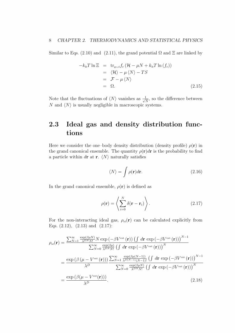
Here we consider the one–body density distribution (density profile) ρ(r) inthe grand canonical ensemble. The quantity ρ(r)dr is the probability to finda particle within dr at r. 〈N〉 naturally satisfies
〈N〉 =
∫ρ(r)dr. (2.16)
In the grand canonical ensemble, ρ(r) is defined as
ρ(r) =
⟨N∑
i=0
δ(r− ri)
⟩. (2.17)
For the non-interacting ideal gas, ρid(r) can be calculated explicitly fromEqs. (2.12), (2.13) and (2.17):
ρid(r) =
∑∞N=1
exp(βµN)λDNN !
N exp (−βV ext (r))(∫
dr exp (−βV ext (r)))N−1
∑∞N=0
exp(βµ)λDNN !
(∫dr exp (−βV ext (r))
)N
=exp (β (µ− V ext (r)))
λD
∑∞N=1
exp(βµ(N−1))
λD(N−1)(N−1)!
(∫dr exp (−βV ext (r))
)N−1
∑∞N=0
exp(βµN)λDNN !
(∫dr exp (−βV ext (r))
)N
=exp (β(µ− V ext(r)))
λD. (2.18)
2.4. CLASSICAL DENSITY FUNCTIONAL THEORY 9
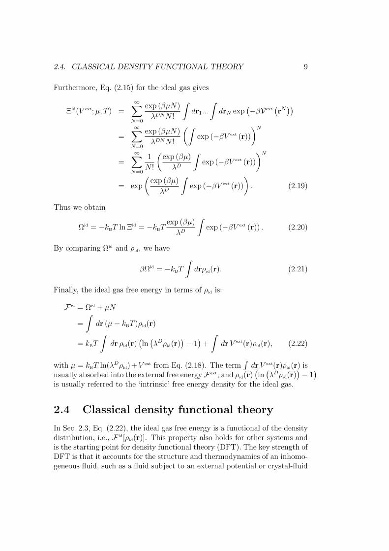
Furthermore, Eq. (2.15) for the ideal gas gives
Ξid(V ext;µ, T ) =∞∑
N=0
exp (βµN)
λDNN !
∫dr1...
∫drN exp
(−βV ext
(rN))
=∞∑
N=0
exp (βµN)
λDNN !
(∫exp (−βV ext (r))
)N
=∞∑
N=0
1
N !
(exp (βµ)
λD
∫exp (−βV ext (r))
)N
= exp
(exp (βµ)
λD
∫exp (−βV ext (r))
). (2.19)
Thus we obtain
Ωid = −kBT ln Ξid = −kBTexp (βµ)
λD
∫exp (−βV ext (r)) . (2.20)
By comparing Ωid and ρid, we have
βΩid = −kBT
∫drρid(r). (2.21)
Finally, the ideal gas free energy in terms of ρid is:
F id = Ωid + µN
=
∫dr (µ− kBT )ρid(r)
= kBT
∫dr ρid(r)
(ln(λDρid(r)
)− 1)
+
∫drV ext(r)ρid(r), (2.22)
with µ = kBT ln(λDρid)+V ext from Eq. (2.18). The term∫drV ext(r)ρid(r) is
usually absorbed into the external free energy F ext, and ρid(r)(ln(λDρid(r)
)− 1)
is usually referred to the ‘intrinsic’ free energy density for the ideal gas.
2.4 Classical density functional theory
In Sec. 2.3, Eq. (2.22), the ideal gas free energy is a functional of the densitydistribution, i.e., F id[ρid(r)]. This property also holds for other systems andis the starting point for density functional theory (DFT). The key strength ofDFT is that it accounts for the structure and thermodynamics of an inhomo-geneous fluid, such as a fluid subject to an external potential or crystal-fluid
10 CHAPTER 2. THERMODYNAMICS AND STATISTICAL PHYSICS
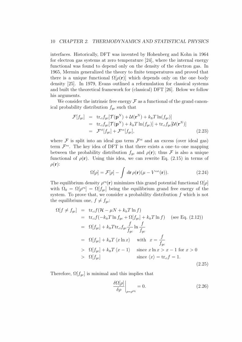
interfaces. Historically, DFT was invented by Hohenberg and Kohn in 1964for electron gas systems at zero temperature [24], where the internal energyfunctional was found to depend only on the density of the electron gas. In1965, Mermin generalized the theory to finite temperatures and proved thatthere is a unique functional Ω[ρ(r)] which depends only on the one–bodydensity [25]. In 1979, Evans outlined a reformulation for classical systemsand built the theoretical framework for (classical) DFT [26]. Below we followhis arguments.
We consider the intrinsic free energy F as a functional of the grand canon-ical probability distribution fgc such that
F [fgc] = trclfgc[T (pN) + U(rN) + kBT ln(fgc)]
= trclfgc[T (pN) + kBT ln(fgc)] + trclfgc[U(rN)]
= F id[fgc] + F ex[fgc], (2.23)
where F is split into an ideal gas term F id and an excess (over ideal gas)term F ex. The key idea of DFT is that there exists a one–to–one mappingbetween the probability distribution fgc and ρ(r); thus F is also a uniquefunctional of ρ(r). Using this idea, we can rewrite Eq. (2.15) in terms ofρ(r):
Ω[ρ] = F [ρ]−∫
dr ρ(r)(µ− V ext(r)). (2.24)
The equilibrium density ρeq(r) minimizes this grand potential functional Ω[ρ]with Ω0 = Ω[ρeq] = Ω[fgc] being the equilibrium grand free energy of thesystem. To prove that, we consider a probability distribution f which is notthe equilibrium one, f 6= fgc:
Ω[f 6= fgc] = trclf(H− µN + kBT ln f)
= trclf(−kBT ln fgc + Ω[fgc] + kBT ln f) (see Eq. (2.12))
= Ω[fgc] + kBT trclfgcf
fgcln
f
fgc
= Ω[fgc] + kBT 〈x lnx〉 with x =f
fgc> Ω[fgc] + kBT 〈x− 1〉 since x lnx > x− 1 for x > 0
> Ω[fgc] since 〈x〉 = trclf = 1.
(2.25)
Therefore, Ω[fgc] is minimal and this implies that
δΩ[ρ]
δρ
∣∣∣∣ρ=ρeq
= 0. (2.26)

2.4. CLASSICAL DENSITY FUNCTIONAL THEORY 11
By inserting Eq. (2.24) into Eq. (2.26), and decomposing F into the ideal gaspart F id (Eq. (2.22)) and the excess free energy F ex, we obtain the importantresult:
λDρeq = exp
(βµ− βδF ex
δρ
∣∣∣∣ρ=ρeq
− βV ext
). (2.27)
The remaining crucial problem is how to obtain or to approximate F ex? InChapter 3, starting from the low density limit, we introduce the Ramakrishnan-Yussouff approximation, the mean–field approximation and the fundamentalmeasure theory. Further, in Chapter 6, a novel machine–learning methodis introduced. The new machine–learning architecture, an adoption of theequation learner of Ref. [1], is capable of generating a functional by usingdensity distributions from simulations/experiments.

Chapter 3
Approximating the excess freeenergy
3.1 Density expansion and direct correlation
function
The excess free energy F ex is a generating functional for a hierarchy of directcorrelation functions (dcf):
C(n)(r1, r2, ..., rn) = −β δnF ex[ρ]
δρ(r1) δρ(r2)...δρ(rn). (3.1)
Usually, the first–order dcf
C(1)(r1) = −β δFex[ρ]
δρ(r1), (3.2)
as already used in Eq. (2.27), and the second–order dcf
C(2)(r1, r2) =δC(1)(r1)
δρ(r2)= −β δ2F ex[ρ]
δρ(r1) δρ(r2)(3.3)
are more useful than the other higher order dcf, and thus we refer to C(2) as‘the dcf’ for short. The connection between the direct correlation functionand the Ornstein–Zernike relation is introduced in the next section. Expand-ing F ex around a homogeneous reference state with ρ(r) = ρ0 gives
F ex[ρ] = F ex[ρ0] +
∫dr1
δF ex[ρ]
δρ(r)
∣∣∣∣ρ=ρ0
∆ρ(r1)
+1
2
∫ ∫dr1dr2
δ2F ex[ρ]
δρ(r1) δρ(r2)
∣∣∣∣ρ=ρ0
∆ρ(r1)∆ρ(r2) + ... (3.4)
13

14 CHAPTER 3. APPROXIMATING THE EXCESS FREE ENERGY
with ∆ρ(r) = ρ(r) − ρ0. Further, since the reference state is homogeneous,
− 1βC(1)(r) = δFex[ρ]
δρ(r)
∣∣∣∣ρ=ρ0
is a constant and thus
F ex[ρ] 'F ex[ρ0]− 1
βC(1)
∫dr ∆ρ(r)
− 1
2β
∫ ∫dr1dr2C
(2)(|r1 − r2|; ρ0)∆ρ(r1)∆ρ(r2). (3.5)
Eq. (3.5) is known as the Ramakrishnan-Yussouff approximation [27] andC(2)(|r1 − r2|; ρ0) could be determined through the pair correlation functionvia the Ornstein–Zernike relation, where the pair correlation function can bedetermined in simulations or experiments (see the next section or Ref. [23] fordetails). Furthermore, it can be shown that −1
βC(2) behaves asymptotically
as the pair potential when r → ∞ [23], if the potential has a long–rangedpart. Therefore, by further approximating C(2)(|r1−r2|; ρ0) with the effectivepair potential ψ(|r1 − r2|), Eq. (3.5) gives
F ex[ρ] ' 1
2
∫ ∫dr1dr2 ψ(|r1 − r2|)ρ(r1)ρ(r2), (3.6)
which is the well–known mean–field or random–phase approximation. WhileEqs. (3.5) and (3.6) are applicable for low densities and weak interactions,the approximation fails in many interesting cases. To improve that, one cansplit ψ into a short–ranged part and a tail part: ψ = ψsr + ψtail. The excessfree energy related to ψtail is approximated by Eq. (3.6) and the excess freeenergy related to ψsr is a functional F ex
ref[ρ] of a new reference system, whichrequires further investigations.
Since the reference part comes from the short–ranged interaction, in themost case it is a harsh repulsive interaction. The simplest approximation forsuch interaction is hard–sphere (HS) interaction, where overlap is forbidden,i.e. for HS,
ψHR(r) =
∞ if |r| < σ
0 otherwise
with σ the (effective) particle diameter. In Sec 3.3, the most accurate func-tional for hard spheres, fundamental measure theory (FMT), is briefly intro-duced.
3.2 Ornstein–Zernike relation
The Ornstein–Zernike (OZ) relation basically describes the relation betweenthe pair correlation function and the dcf. To see this, we first define the
3.2. ORNSTEIN–ZERNIKE RELATION 15
density–density correlation function
H(2)(r1, r2) =⟨
[ρ (r1)− 〈ρ (r1)〉] [ρ (r2)− 〈ρ (r2)〉]⟩
= ρ(2) (r1, r2) + ρ (r1) δ (r1 − r2)− ρ(r1)ρ(r2)
= ρ(r1)ρ(r2)h(2)(r1, r2) + ρ (r1) δ (r1 − r2) , (3.7)
where ρ(2)(r1, r2) =⟨∑
ij,i6=j δ (ri − r1) δ (rj − r2)⟩
and h(2) is the total cor-
relation function (the pair correlation g(2) = h(2) + 1). One can prove [23]that
−βH(2)(r1, r2) =δ2Ω
δφ (r1) δφ (r2)(3.8)
where φ(r) = µ− V ext(r). From Eq. (3.2), we have
βφ(r) = βδF [ρ]
δρ(r)= ln
(λDρ(r)
)− C(1)(r), and
βδφ(r1)
δρ(r2)=
1
ρ(r1)δ(r1 − r2)− C(2)(r1, r2). (3.9)
Combining Eqs. (2.24) and (3.8) we obtain an algebraic
ρ(r) = − δΩ
δφ(r), and βH(2)(r1, r2) =
δρ(r1)
δφ(r2). (3.10)
Through the relation:
δ(r1 − r2) =δρ(r1)
δρ(r2)=
∫dr3
δρ(r1)
δφ(r3)
δφ(r3)
δρ(r2)(3.11)
and substituting δρδφ
by Eq. (3.7) and δφδρ
by Eq. (3.10), we obtain the OZrelation:
h(2)(r1, r2) = C(2)(r1, r2) +
∫dr3C
(2)(r1, r3)ρ(r3)h(2)(r3, r2)
= C(2)(r1, r2) +
∫dr3C
(2)(r1, r3)ρ(r3)C(2)(r3, r2)
+
∫ ∫dr3dr4C
(2)(r1, r3)ρ(r3)C(2)(r3, r4)ρ(r4)C(2)(r4, r2) + ...
(3.12)
Eq (3.12) has a clear physical interpretation: the total correlation h(2) be-tween particles 1 and 2 is due to the direct correlation C(2)(r1, r2) and the

16 CHAPTER 3. APPROXIMATING THE EXCESS FREE ENERGY
‘indirect’ correlation propagated via intermediate particles. For a homoge-neous fluid, Eq. (3.12) can be reduced to
h(2)(r) = C(2)(r) + ρ
∫dr′C(2)(|r− r′|)h(2)(|r′|) (3.13)
where r = |r|. On taking the Fourier transform on both sides, we obtain analgebraic relation between h(2) and C(2):
h(2)(k) = C(2)(k) + ρC(2)(k)h(2)(k)⇒ h(2)(k) =C(2)(k)
1− ρC(2)(k). (3.14)
In experiments or simulations, one could directly determine h(2) or h(2) [23]and thus calculate C(2) for the homogeneous fluid and insert it into theRamakrishnan-Yussouff approximation (Eq. (3.5)).
3.3 Fundamental measure theory
Fundamental measure theory is a special DFT treatment for hard–body flu-ids, using weighted densities. In contrast to approximations by expandingC(2), the free energy density is taken to be a function of several differentweighted densities, defined by geometrical characteristics of the particles.
It can be shown [23] that C(2)(r) in a low-density expansion is given by
C(2)(r) = f(r) + ρf(r)
∫dr′f(|r− r′|)f(|r′|) + ..., (3.15)
where f(r) = e−βψ(r) − 1 is known as the Mayer–f function with ψ theparticle–particle interaction. Thus the excess free energy (F ex) in the lowdensity limit is:
βF ex ' −1
2
∫ ∫d r d r′ρ(r)ρ(r′)f(r− r′). (3.16)
3.3.1 Three–dimensional hard spheres
For hard spheres, f(|r − r′|) = −Θ(2R − |r − r′|) with Θ the Heavisidestep function and R the (effective) radius. By the ingenious insight fromRosenfeld [5], fij can be deconvoluted into a set of weight functions ω 1, suchas
−f(r) = 2 (ω3 ⊗ ω0 + ω2 ⊗ ω1 +ωωω1 ⊗ωωω2) , (3.17)
1For the sake of simplicity, we consider only the one–component case.

3.3. FUNDAMENTAL MEASURE THEORY 17
where
ω3(r) = Θ(R− |r|),ω2(r) = δ(R− |r|),
ω1(r) =ω2(r)
4πR,
ω0(r) =ω2(r)
4πR2,
ωωω2(r) =r
|r|δ(R− |r|), and
ωωω1(r) =ωωω2(r)
4πR, (3.18)
with δ the Dirac delta function. Integrating over the scalar weight functionsgives the ‘fundamental geometric measures” of a sphere,
∫drω3(r) =
3
4πR3 Volumn
∫drω2(r) = 4πR2 Surface
∫drω1(r) = R Mean radius of curvature
∫drω0(r) = 1 Euler characteristic (3.19)
and ωωω2 = Oω3, hence the name “fundamental measure theory”.Eq. (3.16) in the low density limit becomes
βF ex[ρ] =
∫dr Φ([nα]) '
∫dr (n1 n2 − n1 · n2 + n0 n3) (3.20)
with the weighted densities nα(r) = ρ ⊗ ωα =∫dr′ ρ(r′)ωα(r − r′). In
the homogeneous limit, n0 = ρ, n1 = Rρ, n2 = 4πR2ρ, n3 = 43πR3ρ and
n1 = n2 = 0.To approximate the excess free energy density Φ, one possibility, in the
spirit of Eq. (3.20) is to write Φ as a sum of product of weighted densities.One may use a dimensional argument: since βF ex is dimensionless, Φ musthave the dimension of 1/volume, [Φ] = 1
L3 . Thus Φ can only be a sum ofterms consisting of factors n0, n1n2, n1 · n2, n3
2 and n2(n2 · n2), and eachterm can be multiplied with a scalar function fi(n3) . Note [nl] = 1
L3−l . ThusRosenfeld proposed the ansatz:
Φ(nα) = f1(n3)n0 + f2(n3)n1 n2 + f3(n3)n1 ·n2 + f4(n3)n32 + f5(n3)n2(n2 ·n2).
(3.21)
18 CHAPTER 3. APPROXIMATING THE EXCESS FREE ENERGY
Using the definition of the chemical potential µex = δFex
δρ
∣∣∣∣ρ=const.
, we obtain
βµex =∂Φ
∂ρ=∑
α
∂Φ
∂nα
∂nα∂ρ
. (3.22)
We adopt the view of scaled particle (SP) theory, and consider a singlesolute particle of radius Rν in a uniform hard–sphere fluid with radius R. Itcan be shown that [23]
limRν→∞
µex
ν = PspVν (3.23)
with Psp the bulk pressure and Vν the volume of the solute particle, whichleads to
Psp =∂Φ
∂n3
. (3.24)
On the other hand, we have the thermodynamic (TD) relation,
βPTD =−βΩbulk
V= −Φ− βfid + βµρ (3.25)
with fid ideal gas free energy density (Eq (2.22)). Thus we obtain
βPTD = n0 − Φ +∑
α
∂Φ
∂nαnα. (3.26)
By equating PTD and Psp and substituting Eq. (3.21), we obtain
f ′1 = 1 + n3f′1 ⇒ f1 = − ln(1− n3) + C1,
f ′2 = f2 + n3f′2 ⇒ f2 =
C2
1− n3
,
f3 =C3
1− n3
,
f4 =C4
(1− n3)2, and
f5 =C5
(1− n3)2.
(3.27)
In the low density limit, Φ = n1 n2 − n1 · n2 + n0 n3 (Eq. (3.20)) and itleads to C1 = 0, C2 = 1, C3 = −1. Furthermore, considering the dcf for theone–component HS fluid, Eq (3.3) gives
−C(2)(r1, r2) =δ2Φ[n]
δρ (r1) δρ (r2)=∑
α,β
∫dr
∂2Φ
∂nα∂nβwα(r− r1)wβ(r− r2).
(3.28)

3.3. FUNDAMENTAL MEASURE THEORY 19
In the low–density and the homogeneous limit (n2 → 0),
∑
α,β
∫dr
∂2Φ
∂nα∂nβwα(r− r1)wβ(r− r2) =
∑
α,β
∂2Φ
∂nα∂nβwα ⊕ wβ
= Θ(2R− r) + 6C4n2(w2 ⊕ w2) + 2C5n2 (ωωω2 ⊕ωωω2) , (3.29)
where ⊕ denotes the cross–correlation (wα⊕wβ =∫drwα(r−r1)wβ(r−r2))
and
6C4n2(w2 ⊕ w2) + 2C5n2(ωωω2 ⊕ωωω2)
= 2n2(3C4w2 ⊕ w2 + C5ωωω2 ⊕ωωω2)
= 2n2
(4π3 (−C5r
2 − 2 (−3C4 − C5)R2)
r
). (3.30)
To eliminate the divergence at r → 0, we choose C5 = −3C4. To determinethe remaining constant C4, we consider the low–density limit for Φ for ahomogeneous fluid,
Φ =4πR3ρ2
1− 43πR3ρ
+64C4π
3R6ρ3
(1 + 4
3πR3ρ
)2 − ρ ln
[1− 4
3πR3ρ
]
' 16
3πR3ρ2 +
(56π2R6
9+ 64C4π
3R6
)ρ3 +O[ρ4], (3.31)
which gives the equation of state
βPTD
ρ=
1
ρ
(−Φ− βfid +
∂(Φ + fid)
∂ρρ
)
' 1 +16
3πR3ρ+
(112π2R6
9+ 128C4π
3R6
)ρ2 +O[ρ3]. (3.32)
We use the knowledge of the virial expansion with the exactly known firstthree terms,
βP
ρ= 1 + 4η + 10η2 +O[η3], (3.33)
where η = 43πR3ρ is the packing fraction. Putting Eqs. (3.31) and (3.32)
together, we can determine that C4 = 124π
. Finally, we obtain Rosenfeld’sfree energy functional:
Φ = −n0 ln(1− n3) +n1 n2 − n1 · n2
1− n3
+n3
2 − 3n2(n2 · n2)
24π(1− n3)2. (3.34)
20 CHAPTER 3. APPROXIMATING THE EXCESS FREE ENERGY
It is worth to note that in the homogeneous limit, Eq. (3.34) gives the Percus–Yevick–Frisch equation of state [28],
βP
ρ=
1 + η + η2
(1− η)3. (3.35)
Furthermore, we consider an external potential such that the system isheld between two close walls in the x–y–plane, and the local density profileis given by ρ(r) = ρ2D(x, y)δ(z). In this way a homogeneous density pro-file in 2D can be treated as highly confined 3D system, and the free energyF3D[ρ(x, y)δ(z)] = F2D[ρ(x, y)]. Such a narrowing procedure is referred as ‘di-mensional crossover’. By further confinement of the system along the x–axisand all three axes, the local density profile turns into ρ(r) = ρ1D(x)δ(y)δ(z)and ρ(r) = ρ0Dδ(x)δ(y)δ(z). The importance of the cavity–like 0D situa-tion of the latter case is that the crystalline state can be interpreted as ahighly confined inhomogeneous system as each particle confined by its near-est neighborhoods, and thus to capture the crystalline phase the functionalmust have the correct behavior in the 0D limit.
Starting from the exactly known F1D and F0D, Tarazona et al. [6, 7]introduced the tensorial weight function:
ωωωT(r) =
(r · rt|r|2 −
I3
)δ(R− |r|), (3.36)
and the tensor functional:
Φ =− n0 ln(1− n3) +n1 n2 − n1 · n2
1− n3
+n3
2 − 3n2n2 · n2 + 92(nt2 · nT · n2 − Tr(n3
T))
24π(1− n3)2, (3.37)
where I is the unit matrix in R3×3, superscript t represents the transpose,and Tr(·) denotes the trace of a matrix. The tensorial modification givesdecent descriptions of the hard–sphere crystal. However, due to the underly-ing Percus–Yevick–Frisch equation of state, the obtained phase coexistencedensities are lower than the ones from MC simulation results.
White Bear II
In 2006, Hansen–Goos and Roth [29, 8] improved the FMT by considering amodified Carnahan-Starling (CS) equation of state [30] given by
βPCS =n0
1− n3
+n1n2
(1 +
n23
3
)
(1− n3)2+n3
2
(1− 2n3
3+
n23
3
)
12(1− n3)3π. (3.38)
3.3. FUNDAMENTAL MEASURE THEORY 21
In the homogeneous limit for a one–component hard–sphere fluid, Eq. (3.38)is equivalent to the original CS equation of state
βP
ρ=
1 + η + η2 − η3
(1− η)3 , (3.39)
which is more precise than the Percus–Yevick–Frisch equation of state.Equating PCS with PTD and proceeding as before (see Eqs. (3.26) and
(3.27)), we obtain
f2 + n3f′2 =
1 + 13n2
3
(1− n3)2(3.40)
2f4 + n3f′4 =
1− 23n3 + 1
3n2
3
12π(1− n3)3, (3.41)
which gives
f2 =C2
n3
+− 4−1+n3
+ n3 + 2 ln(1− n3)
3n3
(3.42)
f4 =C4
n23
−1−2n3
(−1+n3)2 + n3 + ln(1− n3)
36n23π
. (3.43)
To eliminate the potential divergence in the low–density limit, we chooseC2 = −4
3and C4 = 1
36π; thus, we obtain the White Bear II free energy
functional :
ΦWBIIT
ex,HS (nα) =− n0 ln(1− n3) + g2 (n3)n1 n2 − n1 · n2
1− n3
+ g3 (n3)n3
2 − 3n2n2 · n2
24π(1− n3)2(3.44)
with
g2 (n3) = −(−5 + n3)n3 + 2(−1 + n3) ln(1− n3)
3n3
and
g3 (n3) = −2 (n3(1 + (−3 + n3)n3) + (−1 + n3)2 ln(1− n3))
3n23
. (3.45)
Furthermore, on combining the tensorial modification (Eqs. (3.37)) andWhite Bear II functional (Eq. (3.44)), we obtain the White Bear II tensorialfunctional:
ΦWBII,tensor
ex,HS (nα) = −n0 ln(1− n3) + g2 (n3)n1 n2 − n1 · n2
1− n3
+ g3 (n3)n3
2 − 3n2n2 · n2 + 92(nt2 · nT · n2 − Tr(n3
T))
24π(1− n3)2, (3.46)
which is by far the most accurate functional for HS systems [31, 32].

22 CHAPTER 3. APPROXIMATING THE EXCESS FREE ENERGY
3.3.2 Two–dimensional hard disks
One may expect that FMT for HS systems is capable of describing two–dimensional (2D) hard–disk (HD) systems by a slab–like confinement; how-ever, such confinement gives βP
ρ∼ (1 − η)−5/2 for high packing fractions η,
while the scaled particle theory gives βPρ∼ (1− η)−2 [33]. Alternatively, one
may try to construct F ex by a deconvolution, similarly to Sec.3.3.1 for HDsystems. Then a difficulty arises: the deconvolution of the Mayer functionlike Eq. (3.17) requires an infinite number of weight functions. FollowingRef. [3], the deconvolution for HD is:
−fij(r) = ωi2 ⊗ ωj0 + ωj2 ⊗ ωi0 +∞∑
m=0
Cm2π
ωωωi(m) ⊗ωωωj(m), (3.47)
with weight functions
ωi0(r) =δ(Ri − r)
2πRi
, ωi2(r) = Θ(Ri − r), (3.48)
andωωωi(m)(r) = r...r︸︷︷︸
m times
δ(Ri − r). (3.49)
Using similar arguments as in Sec.3.3.1, one can obtain the excess free energydensity
ΦHD(nα) = −n0 ln(1− n2) +∞∑
m=0
1
4π(1− n2)Cm nm · nm, (3.50)
where the first three coefficients are C0 = π2, C1 = −1 and C2 = −π
4. The
virial expansion of the equation of state for the HD fluid reads βPρ
= 1+2η+
O[ρ2] with packing fraction η = πR2ρ. Unfortunately, the truncation up toC2 gives βP
ρ= 1 + (1 +C0 +C2/2)η+O[ρ2] = 1 + (1 + 3π
8)η+O[ρ2] and thus
fails to deliver the correct second virial coefficient.To cure this deficiency, Roth et al. [3] reconsidered C0..C2 as free parameters.The correct second virial coefficient requires C0 + C2/2 = 1 and the correctfree energy in the 0D confinement for sharp density peak requires C0 +C1 +C2 = 0 (see Sec.3.3.1). Thus the final form of the free energy functional is:
ΦHD(nα) = −n0 ln(1− n2) +(C0n
20 + C1n
21 + C2 Tr[n2
2])
4π(1− n2), (3.51)
with
C0 =a+ 2
3, C1 =
a− 4
3and C2 =
2− 2a
3. (3.52)

3.3. FUNDAMENTAL MEASURE THEORY 23
For the one–component HD system, a best fit to the Mayer f–bond gives a =11/4 whereas a fit to crystal pressures obtained by simulations gives a = 3 [3].For binary systems in the fluid phase, the functional delivers an excellentdescription of pair correlation functions when compared to experiments [12].
3.3.3 One–dimensional hard rods
The deconvolution of the Mayer f function for hard rods (HR) in one dimen-sion (1D) reads
−fij(r) = ωi1 ⊗ ωj0 + ωj1 ⊗ ωi0, (3.53)
where ω1(x) = Θ(σ/2− |x|) and ω0(x) = 12δ(σ/2− |x|). The F ex in the low
density limit is given by
βF ex =
∫n0n1 dx. (3.54)
With the dimensional argument similar to 3D hard-spheres, the ansatz isΦ[n] = n0f(n1). Considering the exact HR equation of state P = ρ
1−ρσand scaled particle theory (Eq. (3.24)), one obtains f ′(n1) = 1
1−n1and thus
f(n1) = − ln(1− n1). The final form of FHR is
βFHR =
∫Φ[n] dx =
∫−n0 ln(1− n1) dx, (3.55)
which is equivalent to the exact HR functional derived by Percus with dif-ferent means in Ref. [34].


Chapter 4
Bulk fluid and crystal phase forone–component hard disks
Here we focus on the one–component two–dimensional (2D) systems of harddisks (HD). The fluid–crystal transition in 2D systems of HD has been offundamental interest over years. Only recently, it has been established inthe one–component system by simulations [10] and experiments [11] that thetransition happens via a first–order transition from the fluid to the hexaticphase and a continuous transition from the hexatic to the crystal phase. Al-though the crystal phase is not strictly periodic (it does not have infinitelylong–ranged translational order), in simulations and experiments it has prac-tically the appearance of a conventional, periodic crystal. Therefore, 2D harddisks have a similar status as a model system for crystallization in films andmonolayers as 3D hard spheres have for crystallization in the bulk. Besidessimulations, classical density functional theory (DFT) for hard particle sys-tems has reached a maturity and accuracy owing to the development of fun-damental measure theory (FMT), starting with the work of Rosenfeld [4]. For2D hard disks, a functional has been proposed in Ref. [3] (see also Sec. 3.3.2),which gives a very accurate description of fluid structure [12], as well as val-ues for the fluid and crystal coexistence densities which are rather close to theones of the first–order fluid–hexatic transition [3]. In these FMT calculations,strict periodicity of the crystal phase was assumed.
25

26 CHAPTER 4. ONE–COMPONENT HARD DISKS
4.1 Bulk phase and coexistence
4.1.1 Bulk phase
In DFT, the bulk fluid phase is characterized by a homogeneous density fieldand the bulk crystal phase is a fluid with spontaneous symmetry breaking,resulting in a strongly peaked density at lattice sites. To study the bulk crys-tal phase and coexistence, we assume periodicity and consider a rectangularunit cell with side lengths L and
√3L for a triangular lattice (see Fig.4.1).
The free parameters in this free energy minimization problem are the densityprofiles ρ(r) in the unit cell as well as the length L. We parametrize the lattervia an effective vacancy concentration nvac:
∫
cell
dr ρ(r) =: 2(1− nvac) = ρ√
3L2. (4.1)
In the one–component case, an ideal crystal has 2 particles in the unit cell,therefore nvac > 0 indeed corresponds to the vacancy concentration in theequilibrium crystal.
ρσ2
L
√3L
1
2
3
4
5
6
7
Figure 4.1: Density distribution ρ(r) of a one–component perfect crystal(ρσ2 = 0.932, nvac = 0.0122, a = 11/4 and σ the hard–disk diameter). Thesolid white line indicates the computational box (rectangular unit cell of thetriangular lattice which contains two particles)
The full minimization of free energy F for given average densities ρ pro-ceeds via
F(ρ) = minnvac
minρ(r)
F [nα], (4.2)

4.1. BULK PHASE AND COEXISTENCE 27
i.e. in two steps [31]. The first minimization step is achieved by an iterativesolution of the Euler–Lagrange equation (for fixed nvac, L)
ρ = exp
(−β δF
ex [nα]
δρ+ βµ
)= K[ρ], (4.3)
where
βδF ex [nα]
δρ(r)=
∫dr′∑
α
∂Φ[nα]
∂nα(r′)wα(r′ − r) (4.4)
with Φ in Eq. (3.51). The chemical potential µ is adapted in each iterationstep to keep the average particle density ρ constant. Iteration is done by usinga combination of Picard steps and discrete inversion in iterative subspace(DIIS) [35, 31] (see also Appendix B for more details). The Picard steps areperformed according to
ρj+1 = ξ K[ρj] + (1− ξ)ρj, (4.5)
where j labels the iteration step and ξ is a Picard mixing parameter whichwe chose in the range from 10−3 to 10−2 for bulk crystal and also interfaceminimizations. The DIIS steps are performed using between 5 and 9 forwardprofiles. The second minimization step, the minimization with respect to nvac
(and thus L), amounts to doing the first minimization for a few values of nvac
within an interval of starting width ∼ 10−3 and subsequently determining theminimum via a quadratic fit. The procedure is iterated with smaller intervalwidths until we have reached 3 digits of confidence or the interval width isless than 10−5 (see Fig. 4.2(a)).
4.1.2 Coexistence
From Table 4.1 we see that coexisting packing fractions and the surfacetension are described very well by FMT, even though in FMT the strictperiodicity assumption for the crystal differs from the character of the hexaticand crystal phase in experiments/simulations. This good correspondence isin line with the quantitative description of fluid structure found in earlierworks [3, 12].
Phase coexistence requires Pcr = Pfl and µcr = µfl. Fully minimizing F/Nwith respect to nvac delivers Pcr and µcr. Through µcr = µfl and the fluidequation of state we can find Pfl and ρfl in the fluid. In general, Pfl 6= Pcr andthus we change ρcr iteratively until βσ2
l |Pcr−Pfl| < 5×10⁻⁶ (see Fig. 4.2(b)).

28 CHAPTER 4. ONE–COMPONENT HARD DISKS
0.010 0.012 0.014 0.016 0.018 0.020
nvac
10−4
10−3
βF/N
+2.9138
1st2nd3rd4th
0.7298 0.7306 0.7314 0.7322
ηcr
−0.0035
−0.0028
−0.0021
−0.0014
−0.0007
0.0000
βσ2∆P
Figure 4.2: (a) Minimization with respect to nvac with ηcr = 0.73 anda = 11/4 (see Eq. 3.52). The procedure is iterated four times. (b)Findingcoexistence pressure by determining ∆P = |Pcr − Pfl| for different ηcr, andthe nvac of each ηcr is determined as in (a).
Table 4.1: Thermodynamic properties of the one–component crystal. σ is theHD diameter, P pressure, µ chemical potential, η = (π/4)σ2ρ packing frac-tion, and the subscript (co) denotes coexistence of the crystal (cr) and fluid(fl), respectively. Note that for Exp and MC, two values for ηcr correspond tothe packing fraction of the hexatic phase at fluid-hexatic coexistence and thepacking fraction at the hexatic–crystal continuous transition, respectively.The FMT coexistence values differ slightly from those in Ref. [3] which sufferfrom a small numerical error.
FMTExp
[11]∗MC
[10]a = 11/4 a = 3
βσ2Pco 10.84 9.234 9.185
βµco 14.576 12.778
ηcr 0.732 0.7165 0.7/0.73 0.716/0.72
ηfl 0.711 0.6913 0.68 0.700
nvac 0.0122 0.0194 0.001
(∗ see Supplementary Material in Ref. [11])

4.2. PLANAR INTERFACE AND SURFACE TENSION 29
4.2 Planar interface and surface tension
A surface tension in 2D is a line tension defined as Ω+PAL
, where P is thepressure, A is the area of the system and L is the length of the interface.Here we are interested in the planar surface tension γ. In general, γ dependson the angle θ between the crystal and the interface normal. To determineγ(θ), we need to model a stress–free solid [36], but extension of a rectangularpiece of solids subjected to periodic boundary conditions is non-trivial due tolattice symmetry. Here we describe how to determine the stress–free periodicboundary condition for a 2D triangular lattice.
As shown in Fig 4.3a, there are two primitive vectors ~a = (a, 0) and~b = (0,
√3a) in a unit cell, where a is the lattice constant.
These vectors in a rotated unit cell with rotation angle θ are
~a′ = a cos(θ)x+ a sin(θ)y. (4.6)
and~b′ = −
√3a sin(θ)x+
√3a cos(θ)y. (4.7)
~a
~b
(a)
~a′~a′
~a′
~b′−~b′
θ
Lx
~b′
~b′
~b′
~b′
~b′
~b′
~b′
~b′
~a′
Ly
(b)
Figure 4.3: (a) Non–rotated lattice, and (b) rotated lattice. The black dotsare lattice sites. In (b), the blue rectangle indicates one periodic unit cell forθ = arctan( 1
3√
3) with (M,N) = (3, 1), (I, J) = (1, 9).

30 CHAPTER 4. ONE–COMPONENT HARD DISKS
In order to exactly fit a periodic structure into the numerical box, thedimension of the numerical box must accommodate multiples of these twobasis vectors (an example is shown in Fig. 4.3b). Thus we have M~a′−N~b′ =Lxx + 0y and I~a′ + J~b′ = 0x + Lyy where M , N , I and J are integers.From the components of the above vector equations that have a zero on theright–hand side, we obtain two conditions for the θ,
tan(θ) =N√3M
=
√3I
J(4.8)
Having four integers fulfilling NM
= 3IJ
, the dimensions of the numerical boxand angle of rotations are given,
Lx =(M~a′ −N~b′
)· x,
Ly =(I~b′ + J~a′
)· y. (4.9)
In Fig. 4.4, we show the free–energy minimized density profiles of interfacewith θ = 0 and θ = arctan( 1
3√
3).
7.5 10.0 12.5 15.0 17.5 20.0 22.5 25.0
x(σ)
1
2
3
4
y(σ)
0.8
1.0
1.2
1.4
ρσ2
(a)
20 25 30 35 40 45 50 55
x(σ)
0
2
4
6
8
10
y(σ)
0.8
1.0
1.2
1.4
ρσ2
(b)
Figure 4.4: Example of (a part of) a planar interface with periodic conditionin the y–direction. The full density profiles are periodic in both the x andy directions. (a) θ = 0, and (b) θ = arctan( 1
3√
3)(NM
= 13, IJ
= 19
). In these
density profiles, the parameters are ηcr = 0.732, ηfl = 0.711 and latticeconstant a = 1.11σ
4.2. PLANAR INTERFACE AND SURFACE TENSION 31
4.2.1 Planar surface tension
For a planar interface in a rectangular numerical box (see Fig. 4.4 showingpart of it), the free energy F can be decomposed into the contribution frombulk phases and interfaces:
F = fliquidLx,liquidLy + fcrystalLx,crystalLy + 2γLy, (4.10)
where Lx,liquid/crystal is the length of the liquid/crystal in the direction of theinterface normal, Ly is the length of the interface, f is the free energy density,and the factor 2 is from the periodic boundary condition.
After dividing both sides of Eq. (4.10) by the area of the simulation boxA = LxLy, the surface tension γ is determined as the slope of the free energydensity versus the inverse length of the numerical box in the direction of theinterface normal Lx with fixed average particle density [37],i.e.,
FA
= fliquid
Lx,liquid
Lx+ fcrystal
Lx,crystal
Lx+ 2γ
1
Lx. (4.11)
Since the average particle density is fixed, we assume thatLx,crystal/liquid
Lxis a
constant for different Lx. Thus the advantage of Eq. (4.11) over Eq. (4.10)is that the precise coexisting free energy densities are not required and γ isdirectly determined by varying Lx.
The density profiles are initialized similar to Ref. [35]. In the iterationswe chose a Picard mixing parameter constant in space and fix the averagedensities ρ = ρcr+ρfl
2by adapting µ in the iterations, where ρcr/fl is the bulk
average density in the crystal/fluid phase at coexistence, and then finallyperform the free minimization.
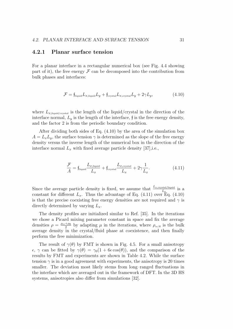
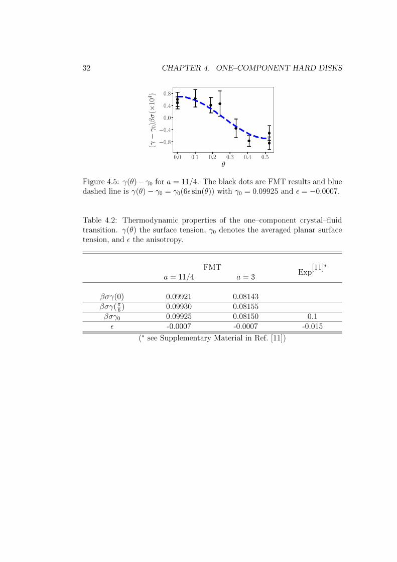
The result of γ(θ) by FMT is shown in Fig. 4.5. For a small anisotropyε, γ can be fitted by γ(θ) = γ0(1 + 6ε cos(θ)), and the comparison of theresults by FMT and experiments are shown in Table 4.2. While the surfacetension γ is in a good agreement with experiments, the anisotropy is 20 timessmaller. The deviation most likely stems from long–ranged fluctuations inthe interface which are averaged out in the framework of DFT. In the 3D HSsystems, anisotropies also differ from simulations [32].
32 CHAPTER 4. ONE–COMPONENT HARD DISKS
0.0 0.1 0.2 0.3 0.4 0.5
θ
−0.8
−0.4
0.0
0.4
0.8
(γ−γ0)βσ(×
104 )
Figure 4.5: γ(θ)− γ0 for a = 11/4. The black dots are FMT results and bluedashed line is γ(θ)− γ0 = γ0(6ε sin(θ)) with γ0 = 0.09925 and ε = −0.0007.
Table 4.2: Thermodynamic properties of the one–component crystal–fluidtransition. γ(θ) the surface tension, γ0 denotes the averaged planar surfacetension, and ε the anisotropy.
FMTExp
[11]∗
a = 11/4 a = 3
βσγ(0) 0.09921 0.08143βσγ(π
6) 0.09930 0.08155
βσγ0 0.09925 0.08150 0.1ε -0.0007 -0.0007 -0.015
(∗ see Supplementary Material in Ref. [11])

4.3. PHASE TRANSITION AND CRYSTAL NUCLEI 33
4.3 Phase transition and crystal nuclei
In the thermodynamic limit (N →∞ and V →∞), the intensive variables,such as the chemical potential µ, must show a horizontal plateau throughoutthe fluid–crystal coexistence region.
However, for a finite size system, the fluid and solid part of the systemarrange such that the interface between the two phases is minimal. Thisbehavior gives rise to topologically different configurations, depending onthe average density ρ. In Fig. 4.6, a schematic sketch of µ(ρ) as a functionof ρ is shown.
The following configurations can be distinguished:
• ρ < ρfl: The stable phase is an undersaturated fluid at these densities.
• ρfl < ρ < ρ1: In a finite system, the fluid is stable, up to a density ρ1,where it becomes metastable. The chemical potential is larger than thecoexistence value, µ > µco.
• ρ1 < ρ < ρ2: A stable nucleus coexists with surrounding fluid. With thedensity increasing, the chemical potential decreases.
• ρ2 < ρ < ρ3: With the density increasing, the nucleus grows and eventuallyconnects to itself over the periodic boundary. A slab configuration formswith two planar interfaces.
• ρ3 < ρ < ρ4: A fluid droplet in a surrounding crystal is formed.
• ρ4 < ρ: For high enough densities, the stable phase is the crystalline phase.In the thermodynamic limit, crystallization starts at a density of ρcr.
Surface tension of crystal nuclei
The surface tension γ plays a crucial role in the free energy barrier for nucle-ation in classical nucleation theory. With the crystal nuclei stabilized in thefinite numerical boxes, we could determine γ versus the size of nuclei. Sincethe anisotropy is small (see Tab. 4.2), we approximate a nucleus as a perfectspherical disk with radius R. The difference of grand potential ∆Ω betweena nucleus and a homogeneous fluid reads
∆Ω = −πR2∆P + γ(R)2πR. (4.12)
Minimizing ∆Ω with respect to R gives
γ(R) = R∆P, (4.13)

34 CHAPTER 4. ONE–COMPONENT HARD DISKS
µ
ρ
µco
ρfl ρ1 ρ2 ρ3 ρ4 ρcr
homogenousfluid fluid + nucleus
fluid+crystalslab crystal+fluid
droplet
crystalline
Figure 4.6: A schematic description of the chemical potential µ(ρ) as a func-tion of ρ. The solid line is a fluid to crystal transition in the thermodynamiclimit. The dashed line and dots are results from FMT equilibrium statesin a finite but large numerical box (64σ × 64σ here). The finite system isinitialized with a disk–shaped nucleus in the center, and the average density(fixed during free energy minimization) is tuned by varying the size of initialthe nucleus and the density of surrounding fluid. The free energy minimiza-tion is performed by using dynamic DFT (see Appendix B for details). Thedensity profiles in the insets are examples of corresponding configurations.
with ∆P = Pcr − Pfl and Pcr/fl the pressure in the nucleus/fluid far frominterface. It is worth to note that Eq. (4.13) is the definition of the Laplacepressure. Thus, the nucleus radius (R) is determined by
∆Ω = πR2∆P. (4.14)
Numerically, ∆Ω = Ωsystem − Ωfl(µeq), where µeq is equilibrium chemical po-tential (not µco). Ωsystem is directly evaluated by the equilibrium densityprofile, and Ωfl(µeq) and Pfl(µeq) are from the equation of state. Pcr is ap-proximated by a unit cell in the middle of the nucleus, since it gives a moreconsistent result than the equation of state.
Using Eqs. (4.13) and (4.14) with ∆P and ∆Ω, we determine R andγ(R) for a nucleus. Furthermore, by varying size and average density of thesystem, we obtain nuclei with different radii. In Fig. 4.7, we show both γ0
γ−1

4.4. HEXATIC PHASE 35
as a function of 1/R and γγ0
as a function of R, and the standard fit with the
Tolman correction [38, 39]:
γ(R)
γ0
' 1
1− δR
⇒ γ0
γ(R)− 1 ' − δ
R(4.15)
with δ the Tolman length.In Fig. 4.7, γ(R) first increases and then decreases as R increases, and
the fit gives δ = 0.9σ. The δ falls in the possible regime (±1σ) from the 3Dhard–sphere DFT studies [40] and the magnitude is close to that determinedfrom the (pseudo) hard–sphere simulations while the sign is different [41, 42].It is difficult to judge the relevance of δ from this work since the sign and themagnitude have been subjest of a longstanding controversy [43, 44, 45, 46, 47]and studies on 2D systems are rare [48].
0.00 0.02 0.04 0.06
1/R(σ)
−0.05
0.00
0.05
0.10
0.15
γ0/γ−1
Tolman
L = 56σ
L = 64σ
L = 72σ
L = 80σ
L = 88σ
L = 96σ
(a)
20 25 30 35 40
R(σ)
0.90
0.95
1.00
1.05
γ/γ
0
Tolman
L = 56σ
L = 64σ
L = 72σ
L = 80σ
L = 88σ
L = 96σ
(b)
Figure 4.7: (a) γ0/γ(R) − 1 versus 1/R, and (b) γ(R)/γ0 versus R. Samecolor dots are same system size (L2). The blue dashed line is a fitting byusing the Tolman correction, which gives δ = 0.9.
4.4 Hexatic phase
The melting transition in 2D, unlike 3D, is proposed to proceed via an addi-tional ‘hexatic’ phase between the fluid and crystalline phase. The hexaticphase is strongly related to the appearance of topological defects. Thereare three main types of defect in 2D HD systems: dislocations, dislocationpairs and disclinations. The dislocation is a pair of five– and seven– foldcoordinated particles (five and seven nearest neighbors), a dislocation pair iscomposed by two dislocations, and a disclination is a single five– or seven–fold coordinated particle.

36 CHAPTER 4. ONE–COMPONENT HARD DISKS
The existence of the hexatic phase is proposed by the KTHNY theory withthe name derived from Kosterlitz, Thouless, Halperin, Nelson, and Young [49,50, 51, 52, 53]; for hard disks, simulations and experiments have proved it in2011 [10] and 2017 [11] respectively. However, to our knowledge, there is nofunctional in DFT so far able to capture the hexatic phase.
Here we briefly describe the melting scenario of 2D melting proposed bythe KTHNY theory. Rigorously speaking, no true crystal exists in 2D due tolong wavelength fluctuations [54], but practically the crystal phase in simula-tions and experiments has the appearance of a conventional periodic crystal.For high packing fractions, 2D HD form a crystalline phase, where the trans-lational order is quasi–long–ranged and the bond–orientational order is long–ranged, and the only type of defect are dislocation pairs. As packing fractiondecreases, dislocation pairs start unbinding and thus destroy the quasi–long–ranged translational order while the long–ranged bond–orientational becomesquasi–long–ranged. This phase is called ‘hexatic phase’. As the packing frac-tion further decreases, dislocations unbind into individual disclinations andboth translational order and bond–orientational order are short–ranged andthe system becomes fluid. In 3D, the unbinding free energy of dislocationpairs is too high thus there is no hexatic phase.
To determine whether the translational order is long or short–ranged, insimulation the vector pair correlation function g(∆r) is used, which is definedas
g(∆r) =V
N2
⟨∑
ij,i6=jδ(∆r− rj + ri)
⟩. (4.16)
To connect with DFT, we consider the two particle density introduced inSec. 3.2,
ρ(2)(r, r′) =
⟨∑
ij,i6=jδ(r− ri)δ(r
′ − rj)
⟩, (4.17)
and rewrite with r′ = r + ∆r,
ρ(2)(r, r + ∆r) =
⟨∑
ij,i6=jδ(r− ri)δ(r + ∆r− rj)
⟩
= ρ(r)ρ(r + ∆r)g(r, r + ∆r). (4.18)
Further, by using the delta function property
∫dr
⟨∑
ij,i6=jδ(r− ri)δ(r + ∆r− rj)
⟩=
⟨∑
ij,i6=jδ (∆r− rj + ri)
⟩, (4.19)
4.4. HEXATIC PHASE 37
we obtain
g(∆r) =V
N2
∫dr ρ(2)(r, r + ∆r) =
V
N2
∫dr ρ(r)ρ(r + ∆r)g(r, r + ∆r).
(4.20)
In the homogeneous system, ρ(2) is independent of r and thus
g(∆r) =V 2
N2ρ2g(∆r) = g(∆r). (4.21)
On the other hand, in an inhomogeneous system, g(r, r + ∆r) depends on rand is unknown in general. Therefore, we assume that g(r, r+∆r) ' 1 when|∆r| 1, and then g(∆r) is the autocorrelation of ρ(r), i.e.
g(∆r) ' V
N2
∫drρ(r)ρ(r + ∆r). (4.22)
The KTHNY theory proposes that g(∆r)− 1 decays algebraically in thecrystalline phase, i.e. proportional to |∆r|−ξ with 1
4< ξ < 1
3, and expo-
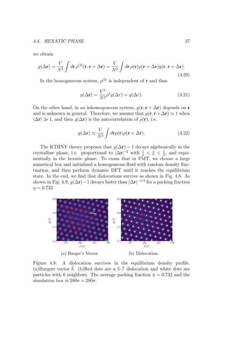
nentially in the hexatic phase. To exam that in FMT, we choose a largenumerical box and initialized a homogeneous fluid with random density fluc-tuation, and then perform dynamic DFT until it reaches the equilibriumstate. In the end, we find that dislocations survive as shown in Fig. 4.8. Asshown in Fig. 4.9, g(∆r)−1 decays faster than |∆r|−1/3 for a packing fractionη = 0.732.
227 230 233 236x(σ)
174
177
180
183
y(σ)
~b
(a) Burger’s Vector
227 230 233 236x(σ)
174
177
180
183
y(σ)
(b) Dislocation.
Figure 4.8: A dislocation survives in the equilibrium density profile.(a)Burgers vector ~b. (b)Red dots are a 5–7 dislocation and white dots areparticles with 6 neighbors. The average packing fraction η = 0.732 and thesimulation box is 280σ × 280σ.

38 CHAPTER 4. ONE–COMPONENT HARD DISKS
101 102
|∆r/σ|10−2
10−1
100
101
g(∆
r)−1
∝ |∆r|−1/3
Figure 4.9: Log–log plot for g(∆r)− 1 as a function of |∆r|. The red dashedline is the stable limit purposed by KTHNY theory. The average packingfraction η = 0.732 and the numerical box is 280σ × 280σ.
However, there are several issues. First, we can not rule out that thedislocations result from mechanical stress. As the numeric box is square inthis case (280σ × 280σ), it can not fit a perfect equilibrium crystal and thestress must result in a distorted crystal or in dislocations, and both casesare possible local minimums. In simulations, the simulation boxes go up to∼ 1000σ × 1000σ to eliminate the influence of stress. Second, for higherpacking fractions, we are not sure whether g(∆r) − 1 decays algebraicallyand dislocation pairs exist or not. Third, in DFT, a density profile shouldbe an ensemble average and can be viewed as an average of snapshots insimulations/experiments. With dislocations fluctuating (moving around) insimulations, the corresponding density profile should be crystal–like withhigh vacancy concentration; thus, the ‘explicit’ dislocation shown in Fig. 4.8means it is trapped locally, which differs from the simulation picture. Fourth,we are unsure how dislocations contribute to the free energy. That is to say,if dislocations or interaction among dislocations can contribute negative freeenergy in a large system, a crystal with intrinsic dislocations could be favoredover a pure crystalline phase, i.e. Fdislocation + crystal < Fstressed crystal.
Last but not least, the existence of the hexatic phase stems from the ‘in-trinsic’ long–ranged fluctuations [54], but in FMT, as pointed out in Ref. [32],the long–ranged fluctuations in the interface are averaged out; thus it is un-likely to have intrinsic long–ranged fluctuations in 2D FMT. However, toresolve the above mentioned issues, we need even bigger systems, more den-sity profiles with higher/lower density and different initial condition to verifythe existence of the hexatic phase or whether dislocations can survive in alarge system or not; unfortunately this is beyond the limitation of our current

4.5. CONCLUSION 39
computational resources. Fig. 4.9 took more than one month using a NVIDAK40 GPU.
4.5 Conclusion
In this chapter we have shown the FMT free energy functional for the 2D HDsuccessfully delivers an accurate mean surface tension and thermodynamicproperties in comparison with simulations and experiments. However theanisotropy of the surface tension differs up to a factor of 20 comparing tothat from experiments. A possible reason is that DFT smears out the long–ranged fluctuations. Furthermore, we investigate the surface tension of disk–shaped nuclei, γ(R), with R the nucleus radius. The γ(R) first increasesthen decreases as R increases. The Tolman length by the fitting with theTolman correction falls in the possible regime (±1σ) from the 3D hard–sphere DFT studies [40] and the magnitude is close to that determined fromthe hard–sphere simulations while the sign is different [41, 42]. Finally, wehave investigated the existence of the hexatic phase. For η = 0.732, wefind that g(∆r)− 1 decays faster than algebraically while the density profilestill maintains the crystalline structure with dislocations, which is evidenceof the existence of the hexatic phase. However, we are unsure whether thedislocations result from stress, and whether intrinsic long–ranged fluctuationsexist in DFT or not. Thus, further investigations are needed.


Chapter 5
Hard–disk binary mixtures
Partial results of this chapter have been published in: PhysicalReview E 98.1.012608 (2018) with the title “Phase diagrams andcrystal–fluid surface tensions in additive and nonadditive two–dimensional binary hard–disk mixtures”[55]
In this chapter, we employ the FMT functional of Ref. [3] (see alsoSec. 3.3.2) to study phase diagrams and crystal–fluid surface tensions foradditive and nonadditive binary hard–disk mixtures. We consider a mixtureof large (l) and small (s) disks, with diameter σl and σs, respectively, andq = σs
σldenoting the size ratio. In the case of an additive system (denoted as
HD mixture), one may define an interaction diameter dij = σi/2 + σj/2 withi, j = l, s. The pair potential Φij(r) between two particles with center-center distance r is ∞ for r < dij and 0 for r > dij.
On the other hand, we consider a mixture in which the interaction be-tween two small disks is zero, i.e. they behave as an ideal gas and the otherinteractions (large–large and large–small) remain unchanged. This mixture isthe 2D variant [13] of the well–known Asakura–Oosawa (AO) model [14, 15],and we denote this kind of mixtures as AO mixture.
As shown in Fig. 5.1, if the distance of two large disks is less than σl +σs,there will be a overlap of excluded area for small disks; i.e. the small diskswill act as a depletant and induce an effective two–body attractive potentialbetween the large disks. This effect is an example of an entropic force. Inthe case of an AO mixture, the effective potential among large disks can be
41

42 CHAPTER 5. HARD–DISK BINARY MIXTURES
analytically determined (in the low density limit) [14, 13] as:
βΦAO(r) =
∞ if r < σl
−η′[cos−1
(r
σl(1+q)
)− r
σl(1+q)
√1− ( r
σl(1+q))2]
if σl < r < σl + σs
0 otherwise,
(5.1)
where η′ = σ2s
2ρs
(1+qq
)2
determines the magnitude of the depletion potential
(ρs is the bulk number density of small disks). Furthermore, β = 1kBT
, withkB denoting Boltzmann’s constant, and T temperature. For small size ratiosq = σs
σl≤ 2−
√3√
3' 0.155, the AO mixture can be mapped exactly onto a
single component model with an effective two–body potential given by thedepletion potential above. For larger q, the effective potential should includen–body overlaps of excluded area (n ≥ 3). Furthermore, in the dilute limitof the (additive) HD mixture (with the number density ρl of large disks beingsmall), the effective potential between large disks is identical to Eq. (5.1) [13].
Figure 5.1: A schematic plot of entropic force. A dark blue disk is a largeHD with a diameter σl and a red disk is a small disk with a diameter σs. Thelight blue region with dashed circle surrounding every HD is excluded areafor the centers of the small disks. When the HD get close enough, as shownin the center of the plot, the excluded area surrounding the HD intersect.The overlap results in a reduced excluded area, which increases the totalavailable area for small disks and thus the entropy.
5.1. FREE ENERGY FUNCTIONAL 43
5.1 Free energy functional
Here we adapt the 2D FMT (see Sec. 3.3.2) for the free energy functional. Inthe HD case, the only difference is that the weighted densities nα are sumsover convolutions of the HD species density profiles with weight functions,
nα(r) =∑
i=s,l
∫dr′ ρi(r
′)wiα(r− r′) (5.2)
=: nsα + nl
α
where α indicates the type of weight function and i the species (l=large ands=small).
The functional for the AO mixture can be obtained by the ‘linearizationrecipe’: The direct correlation function between two small particles shouldvanish in order to be consistent with the small species behaving as an idealgas, i.e.,
C(2)ss (r, r′) = −β δ2F ex
δρs(r)δρs(r′)!
= 0. (5.3)
In 3D, such a functional (derived from the original Rosenfeld functional [4])describes structural properties and wetting transitions in the fluid phase verywell [56]. According to the linearization recipe, the AO mixture excess freeenergy density is given by
ΦAO(nlα, n
sα
)= ΦHD
(nlα
)+∑α
nsα
∂ΦHD(nlα)
∂nlα
. (5.4)
Furthermore, the small species density profile is computed by the grand–canonical equilibrium condition which can be solved explicitly:
δΩ[ρl, ρs]
δρs
!= 0⇒ ρs(r) = exp
(βµs −
∫dr′∑
α
∂ΦHDex
[nlα]
∂nlα
wsα(r′ − r)
),(5.5)
and the remaining free energy minimization with respect to ρl(r) is similaras in Sec. 4.1.1.
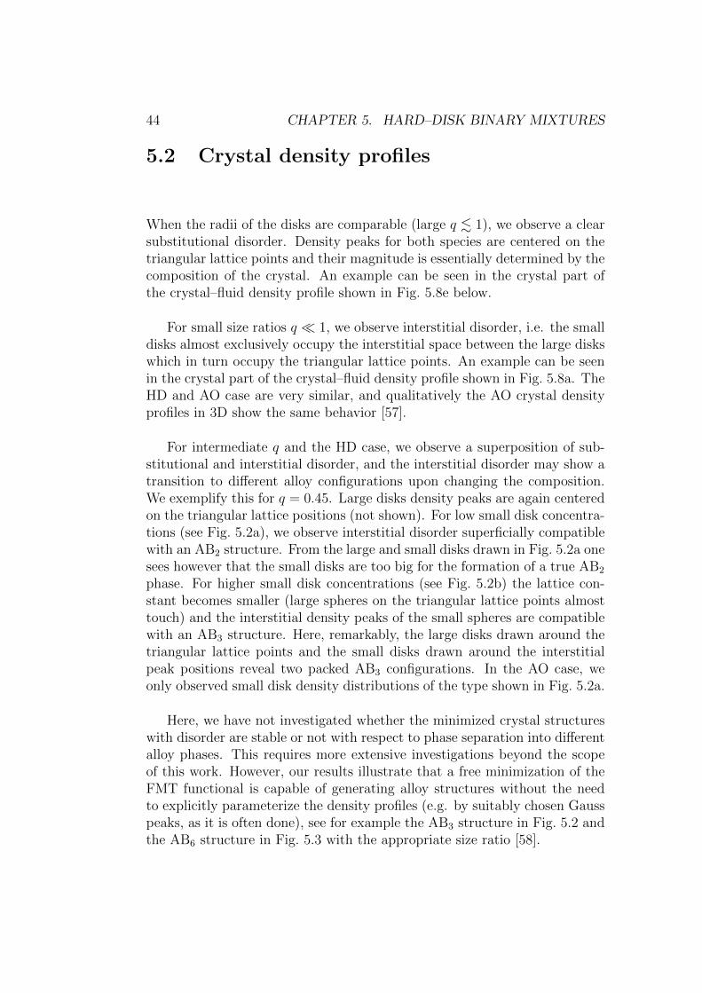
44 CHAPTER 5. HARD–DISK BINARY MIXTURES
5.2 Crystal density profiles
When the radii of the disks are comparable (large q . 1), we observe a clearsubstitutional disorder. Density peaks for both species are centered on thetriangular lattice points and their magnitude is essentially determined by thecomposition of the crystal. An example can be seen in the crystal part ofthe crystal–fluid density profile shown in Fig. 5.8e below.
For small size ratios q 1, we observe interstitial disorder, i.e. the smalldisks almost exclusively occupy the interstitial space between the large diskswhich in turn occupy the triangular lattice points. An example can be seenin the crystal part of the crystal–fluid density profile shown in Fig. 5.8a. TheHD and AO case are very similar, and qualitatively the AO crystal densityprofiles in 3D show the same behavior [57].
For intermediate q and the HD case, we observe a superposition of sub-stitutional and interstitial disorder, and the interstitial disorder may show atransition to different alloy configurations upon changing the composition.We exemplify this for q = 0.45. Large disks density peaks are again centeredon the triangular lattice positions (not shown). For low small disk concentra-tions (see Fig. 5.2a), we observe interstitial disorder superficially compatiblewith an AB2 structure. From the large and small disks drawn in Fig. 5.2a onesees however that the small disks are too big for the formation of a true AB2
phase. For higher small disk concentrations (see Fig. 5.2b) the lattice con-stant becomes smaller (large spheres on the triangular lattice points almosttouch) and the interstitial density peaks of the small spheres are compatiblewith an AB3 structure. Here, remarkably, the large disks drawn around thetriangular lattice points and the small disks drawn around the interstitialpeak positions reveal two packed AB3 configurations. In the AO case, weonly observed small disk density distributions of the type shown in Fig. 5.2a.
Here, we have not investigated whether the minimized crystal structureswith disorder are stable or not with respect to phase separation into differentalloy phases. This requires more extensive investigations beyond the scopeof this work. However, our results illustrate that a free minimization of theFMT functional is capable of generating alloy structures without the needto explicitly parameterize the density profiles (e.g. by suitably chosen Gausspeaks, as it is often done), see for example the AB3 structure in Fig. 5.2 andthe AB6 structure in Fig. 5.3 with the appropriate size ratio [58].

5.2. CRYSTAL DENSITY PROFILES 45
0.0 0.8 1.6
x(σl)
0.0
0.5
1.0
y(σ
l)
ρsσ2l
0.026
0.028
0.030
0.032
0.034
0.036
(a) cs = 0.03
0.0 0.8 1.6
x(σl)
0.0
0.5
1.0
y(σ
l)
ρsσ2l
0.3
0.4
0.5
0.6
0.7
0.8
(b) cs = 0.39
Figure 5.2: Density profiles for small disks in a HD mixture crystal withq = 0.45 at crystal–fluid coexistence for small disk concentration cs = 0.03(a)and cs = 0.39(b), with cs = ρs/(ρs + ρl) . The solid blue circles indicate theextension of large disks, solid and dashed white circles indicate the extensionof small disks. In both cases, the density profile is a superposition of substi-tutional and interstitial disorder. In (b), interstitial disorder dominates andis compatible with an AB3 alloy structure where one large disk is replacedby three small disks (white solid or dashed circles) .
0 1 2x(σl)
0
11
y(σ
l)
ρlσ2l
5
10
15
20
25
(a) ρlσ2l
0 1 2x(σl)
0
1
y(σ
l)
ρsσ2l
5
10
15
20
25
30
35
40
(b) ρsσ2l
Figure 5.3: Density profiles for large and small disks in am AB6 HD mixturecrystal with q ' 0.349. (a) large disks ρlσ
2l . (b) small disks ρsσ
2l .

46 CHAPTER 5. HARD–DISK BINARY MIXTURES
5.3 Phase diagrams
For two–component systems, equilibrium states are on a surface in a three–dimensional space, spanned by e.g. the packing fractions ηl, ηs and thepressure P . Consequently, binodals are lines in this three–dimensional spaceand they are often displayed by their two–dimensional projections, e.g. linesin the ηl–P or cs/l–P plane where cs/l = ρs/l/(ρl + ρs) is the relative concen-tration of small/large spheres. In the AO model, customarily the ηl–µs planeis chosen but the topology of phase diagrams is very similar to the one in theηl–P plane.
For a size ratio q = 0.15, the phase diagram is shown in Fig. 5.4 in two dif-ferent projections. For both HD and AO mixtures, the addition of the smallspecies leads to an increased coexistence pressure for the fluid–crystal tran-sition, i.e. the fluid phase is stabilized. The AO mixture shows the typicalwidening of the coexistence gap (ηl,cr− ηl,fl) with increasing concentration ofthe small species (see Fig. 5.4a), smoothly leading to a sublimation line. Forηs . 0.01, the HD mixture binodal follows the AO binodal, i.e. also showsan initial widening of the coexistence gap. This could be expected since forthese small concentrations the small disks only act as depletants and theirmutual interaction is irrelevant. For higher ηs, the binodals separate. Thechoice of the parameter a in the functional has a significant influence on thelocation of the binodal. This is similar to the observation in Ref. [57] that alsoin the 3D case, the binodal differs considerably between the White Bear II(tensorial) and the Rosenfeld (tensorial) functional, although the differencesin the one–component case are not that significant.
5.3.1 Small size ratios q
For the size ratios q = 0.3 and q = 0.45, the phase diagrams are shownin Fig. 5.5 in the ηl–P plane. For the AO mixture, the liquid (rich in largedisks)–vapor (poor in large disks) transition has become stable which leads tothe appearance of a triple point above which sublimation (the vapor–crystaltransition) is stable. The triple point pressure decreases with increasing q.The difference in the location of the liquid–vapor transition between the FMTresults for the two different values of a is only a consequence of normalizingthe pressure axis by P 1c
co (for the two a values, it differs by ∼ 15%, see Table4.1). For the HD mixtures, there is no fluid–fluid transition and there ishardly any widening of the coexistence gap of the fluid–crystal transitionvisible.
The results for the AO mixture are very similar to the 3D case [57]. Exper-imentally, it is possible to realize such 2D systems by sedimented monolayers
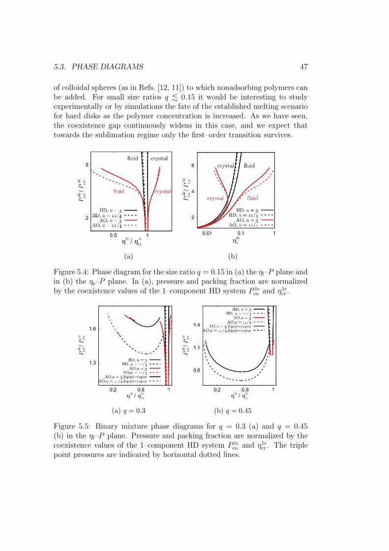
5.3. PHASE DIAGRAMS 47
of colloidal spheres (as in Refs. [12, 11]) to which nonadsorbing polymers canbe added. For small size ratios q . 0.15 it would be interesting to studyexperimentally or by simulations the fate of the established melting scenariofor hard disks as the polymer concentration is increased. As we have seen,the coexistence gap continuously widens in this case, and we expect thattowards the sublimation regime only the first–order transition survives.
(a) (b)
Figure 5.4: Phase diagram for the size ratio q = 0.15 in (a) the ηl–P plane andin (b) the ηs–P plane. In (a), pressure and packing fraction are normalizedby the coexistence values of the 1–component HD system P 1c
co and η1ccr .
(a) q = 0.3 (b) q = 0.45
Figure 5.5: Binary mixture phase diagrams for q = 0.3 (a) and q = 0.45(b) in the ηl–P plane. Pressure and packing fraction are normalized by thecoexistence values of the 1–component HD system P 1c
co and η1ccr . The triple
point pressures are indicated by horizontal dotted lines.
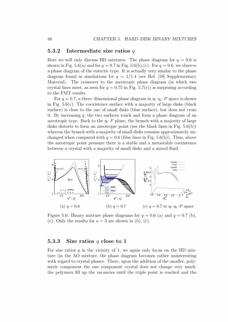
48 CHAPTER 5. HARD–DISK BINARY MIXTURES
5.3.2 Intermediate size ratios q
Here we will only discuss HD mixtures. The phase diagram for q = 0.6 isshown in Fig. 5.6(a) and for q = 0.7 in Fig. 5.6(b),(c). For q = 0.6, we observea phase diagram of the eutectic type. It is actually very similar to the phasediagram found in simulations for q = 1/1.4 (see Ref. [59] SupplementaryMaterial). The crossover to the azeotropic phase diagram (in which twocrystal lines meet, as seen for q = 0.75 in Fig. 5.7(c)) is surprising accordingto the FMT results.
For q = 0.7, a three–dimensional phase diagram in ηl–ηs–P space is shownin Fig. 5.6(c). The coexistence surface with a majority of large disks (blacksurface) is close to the one of small disks (blue surface), but does not crossit. By increasing q, the two surfaces touch and form a phase diagram of anazeotropic type. Back to the ηl–P plane, the branch with a majority of largedisks distorts to form an azeotropic point (see the black lines in Fig. 5.6(b))whereas the branch with a majority of small disks remains approximately un-changed when compared with q = 0.6 (blue lines in Fig. 5.6(b)). Thus, abovethe azeotropic point pressure there is a stable and a metastable coexistencebetween a crystal with a majority of small disks and a mixed fluid.
(a) q = 0.6 (b) q = 0.7
0 0.4
0.8
0 0.2 0.4 0.6 0.8
2
2.5
3
3.5
4
P2
c
co / P
1c
co
Crystal
Fluid
Crystal
Fluid
η2c
l/η cr
1c
η2c
s
P2
c
co / P
1c
co
(c) q = 0.7 in ηl–ηs–P space
Figure 5.6: Binary mixture phase diagrams for q = 0.6 (a) and q = 0.7 (b),(c). Only the results for a = 3 are shown in (b), (c).
5.3.3 Size ratios q close to 1
For size ratios q in the vicinity of 1, we again only focus on the HD mix-ture (in the AO mixture, the phase diagram becomes rather uninterestingwith regard to crystal phases. There, upon the addition of the smaller, poly-meric component the one–component crystal does not change very much:the polymers fill up the vacancies until the triple point is reached and the
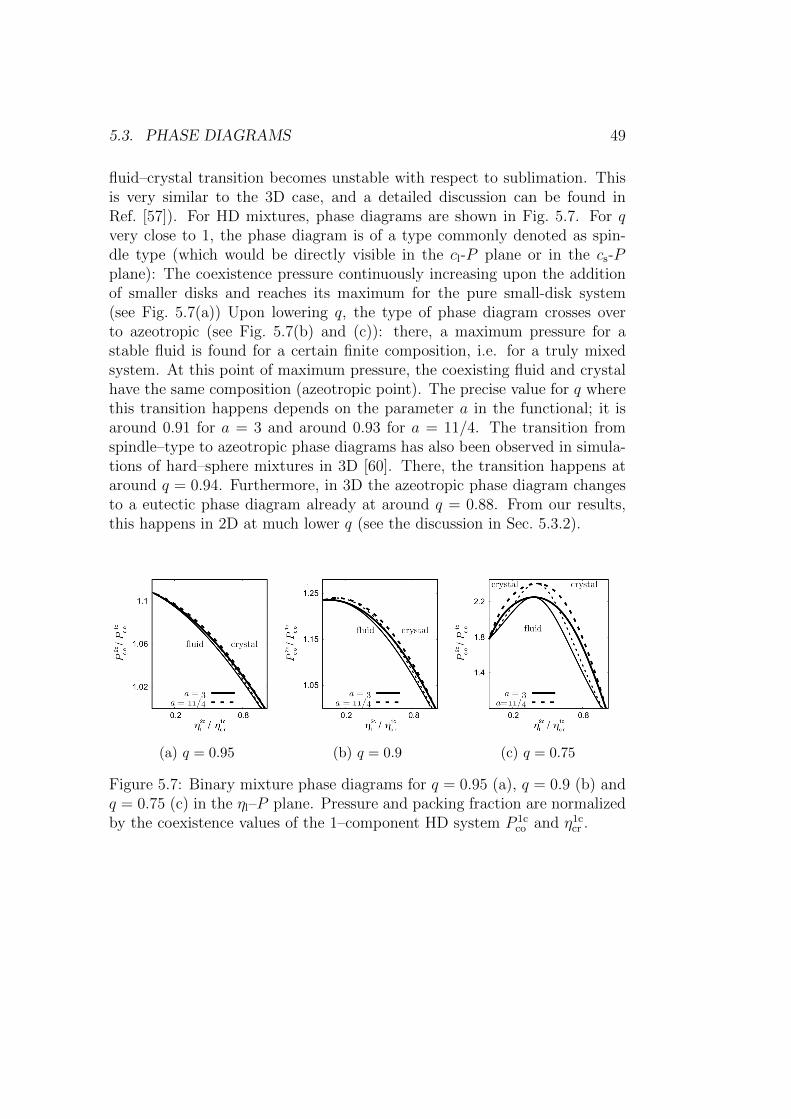
5.3. PHASE DIAGRAMS 49
fluid–crystal transition becomes unstable with respect to sublimation. Thisis very similar to the 3D case, and a detailed discussion can be found inRef. [57]). For HD mixtures, phase diagrams are shown in Fig. 5.7. For qvery close to 1, the phase diagram is of a type commonly denoted as spin-dle type (which would be directly visible in the cl-P plane or in the cs-Pplane): The coexistence pressure continuously increasing upon the additionof smaller disks and reaches its maximum for the pure small-disk system(see Fig. 5.7(a)) Upon lowering q, the type of phase diagram crosses overto azeotropic (see Fig. 5.7(b) and (c)): there, a maximum pressure for astable fluid is found for a certain finite composition, i.e. for a truly mixedsystem. At this point of maximum pressure, the coexisting fluid and crystalhave the same composition (azeotropic point). The precise value for q wherethis transition happens depends on the parameter a in the functional; it isaround 0.91 for a = 3 and around 0.93 for a = 11/4. The transition fromspindle–type to azeotropic phase diagrams has also been observed in simula-tions of hard–sphere mixtures in 3D [60]. There, the transition happens ataround q = 0.94. Furthermore, in 3D the azeotropic phase diagram changesto a eutectic phase diagram already at around q = 0.88. From our results,this happens in 2D at much lower q (see the discussion in Sec. 5.3.2).
(a) q = 0.95 (b) q = 0.9 (c) q = 0.75
Figure 5.7: Binary mixture phase diagrams for q = 0.95 (a), q = 0.9 (b) andq = 0.75 (c) in the ηl–P plane. Pressure and packing fraction are normalizedby the coexistence values of the 1–component HD system P 1c
co and η1ccr .
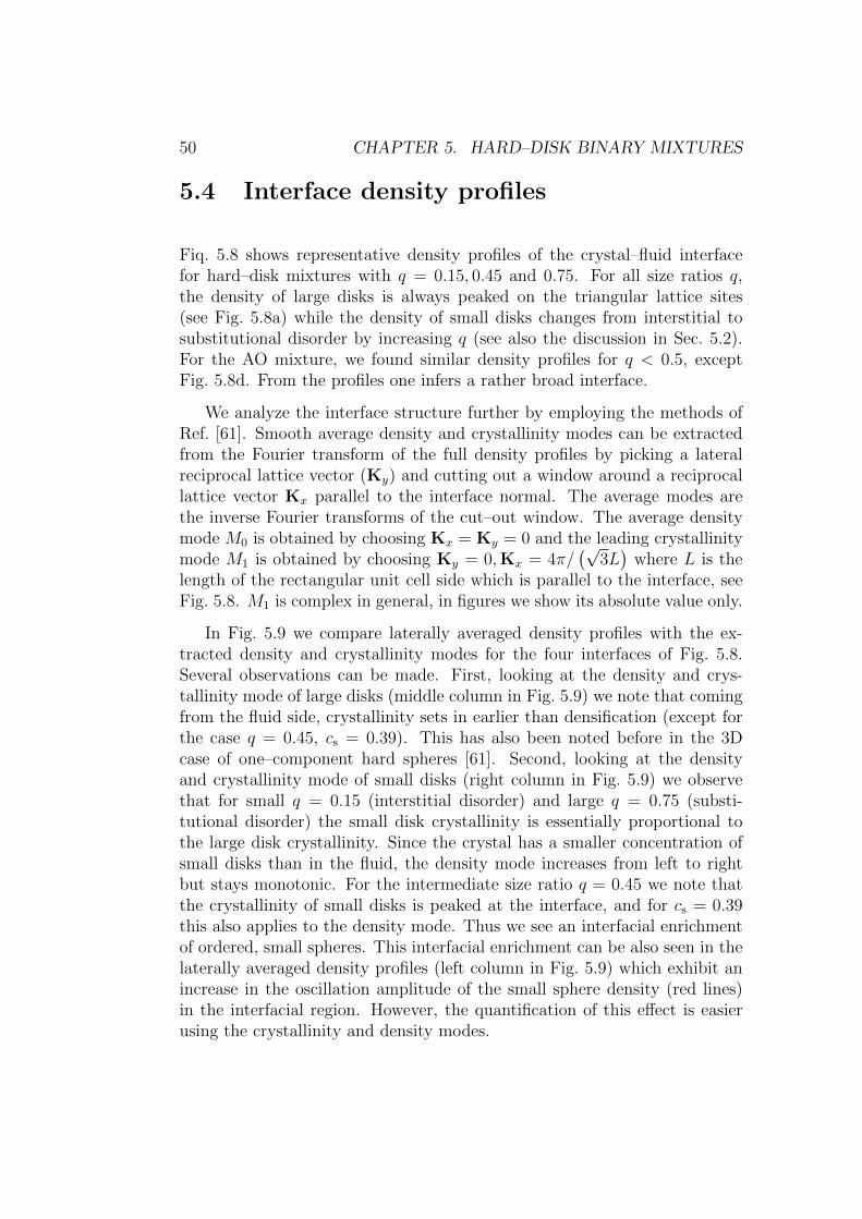
50 CHAPTER 5. HARD–DISK BINARY MIXTURES
5.4 Interface density profiles
Fiq. 5.8 shows representative density profiles of the crystal–fluid interfacefor hard–disk mixtures with q = 0.15, 0.45 and 0.75. For all size ratios q,the density of large disks is always peaked on the triangular lattice sites(see Fig. 5.8a) while the density of small disks changes from interstitial tosubstitutional disorder by increasing q (see also the discussion in Sec. 5.2).For the AO mixture, we found similar density profiles for q < 0.5, exceptFig. 5.8d. From the profiles one infers a rather broad interface.
We analyze the interface structure further by employing the methods ofRef. [61]. Smooth average density and crystallinity modes can be extractedfrom the Fourier transform of the full density profiles by picking a lateralreciprocal lattice vector (Ky) and cutting out a window around a reciprocallattice vector Kx parallel to the interface normal. The average modes arethe inverse Fourier transforms of the cut–out window. The average densitymode M0 is obtained by choosing Kx = Ky = 0 and the leading crystallinitymode M1 is obtained by choosing Ky = 0,Kx = 4π/
(√3L)
where L is thelength of the rectangular unit cell side which is parallel to the interface, seeFig. 5.8. M1 is complex in general, in figures we show its absolute value only.
In Fig. 5.9 we compare laterally averaged density profiles with the ex-tracted density and crystallinity modes for the four interfaces of Fig. 5.8.Several observations can be made. First, looking at the density and crys-tallinity mode of large disks (middle column in Fig. 5.9) we note that comingfrom the fluid side, crystallinity sets in earlier than densification (except forthe case q = 0.45, cs = 0.39). This has also been noted before in the 3Dcase of one–component hard spheres [61]. Second, looking at the densityand crystallinity mode of small disks (right column in Fig. 5.9) we observethat for small q = 0.15 (interstitial disorder) and large q = 0.75 (substi-tutional disorder) the small disk crystallinity is essentially proportional tothe large disk crystallinity. Since the crystal has a smaller concentration ofsmall disks than in the fluid, the density mode increases from left to rightbut stays monotonic. For the intermediate size ratio q = 0.45 we note thatthe crystallinity of small disks is peaked at the interface, and for cs = 0.39this also applies to the density mode. Thus we see an interfacial enrichmentof ordered, small spheres. This interfacial enrichment can be also seen in thelaterally averaged density profiles (left column in Fig. 5.9) which exhibit anincrease in the oscillation amplitude of the small sphere density (red lines)in the interfacial region. However, the quantification of this effect is easierusing the crystallinity and density modes.
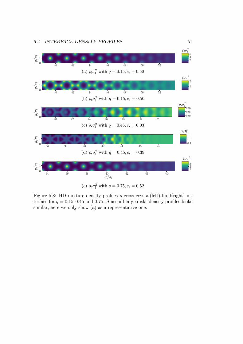
5.4. INTERFACE DENSITY PROFILES 51
40 42 44 46 48 50 52x/σl
0
1
y/σ
l
ρlσ2l
246
(a) ρlσ2l with q = 0.15, cs = 0.50
40 42 44 46 48 50 52x/σl
0
1
y/σ
l
ρsσ2l
1
2
(b) ρsσ2l with q = 0.15, cs = 0.50
40 42 44 46 48 50 52x/σl
0
1
y/σ
l
ρsσ2l
0.03
0.05
0.07
(c) ρsσ2l with q = 0.45, cs = 0.03
36 38 40 42 44 46 48x/σl
0
1
y/σ
l
ρsσ2l
0.4
1.0
1.6
(d) ρsσ2l with q = 0.45, cs = 0.39
34 36 38 40 42 44 46x/σl
0
1
y/σ
l
ρsσ2l
123
(e) ρsσ2l with q = 0.75, cs = 0.52
Figure 5.8: HD mixture density profiles ρ cross crystal(left)-fluid(right) in-terface for q = 0.15, 0.45 and 0.75. Since all large disks density profiles lookssimilar, here we only show (a) as a representative one.

52 CHAPTER 5. HARD–DISK BINARY MIXTURES
(a) q = 0.15, cs = 0.50
(b) q = 0.45, cs = 0.03
(c) q = 0.45, cs = 0.39
(d) q = 0.75, cs = 0.52
Figure 5.9: Laterally averaged density profiles (left column), density andleading crystallinity modes of large disks (middle column) and small disks(right column) for the four interfaces of Fig. 5.8. Black lines refer to largedisks, red lines to small disks. In the middle and right column, full lines aredensity modes M0 and dashed lines crystallinity modes M1.
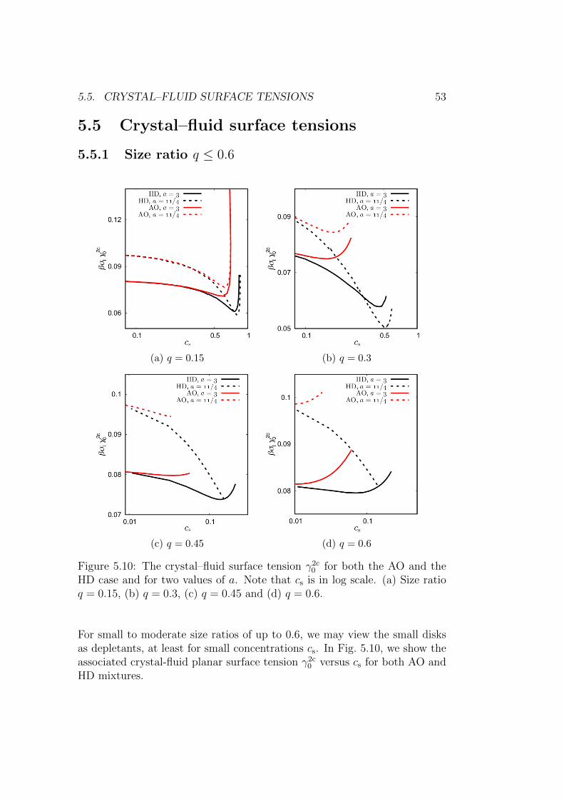
5.5. CRYSTAL–FLUID SURFACE TENSIONS 53
5.5 Crystal–fluid surface tensions
5.5.1 Size ratio q ≤ 0.6
(a) q = 0.15 (b) q = 0.3
(c) q = 0.45 (d) q = 0.6
Figure 5.10: The crystal–fluid surface tension γ2c0 for both the AO and the
HD case and for two values of a. Note that cs is in log scale. (a) Size ratioq = 0.15, (b) q = 0.3, (c) q = 0.45 and (d) q = 0.6.
For small to moderate size ratios of up to 0.6, we may view the small disksas depletants, at least for small concentrations cs. In Fig. 5.10, we show theassociated crystal-fluid planar surface tension γ2c
0 versus cs for both AO andHD mixtures.
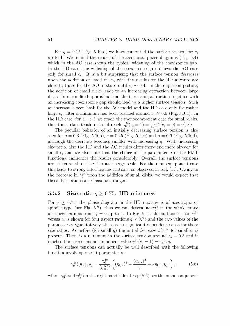
54 CHAPTER 5. HARD–DISK BINARY MIXTURES
For q = 0.15 (Fig. 5.10a), we have computed the surface tension for cs
up to 1. We remind the reader of the associated phase diagrams (Fig. 5.4)which in the AO case shows the typical widening of the coexistence gap.In the HD case, the widening of the coexistence gap follows the AO caseonly for small cs. It is a bit surprising that the surface tension decreasesupon the addition of small disks, with the results for the HD mixture areclose to those for the AO mixture until cs ∼ 0.4. In the depletion picture,the addition of small disks leads to an increasing attraction between largedisks. In mean–field approximation, the increasing attraction together withan increasing coexistence gap should lead to a higher surface tension. Suchan increase is seen both for the AO model and the HD case only for ratherlarge cs, after a minimum has been reached around cs ≈ 0.6 (Fig.5.10a). Inthe HD case, for cs → 1 we reach the monocomponent case for small disks,thus the surface tension should reach γ2c
0 (cs = 1) = σl
σsγ2c
0 (cs = 0) = γ1c0 /q.
The peculiar behavior of an initially decreasing surface tension is alsoseen for q = 0.3 (Fig. 5.10b), q = 0.45 (Fig. 5.10c) and q = 0.6 (Fig. 5.10d),although the decrease becomes smaller with increasing q. With increasingsize ratio, also the HD and the AO results differ more and more already forsmall cs and we also note that the choice of the parameter a in the FMTfunctional influences the results considerably. Overall, the surface tensionsare rather small on the thermal energy scale. For the monocomponent casethis leads to strong interface fluctuations, as observed in Ref. [11]. Owing tothe decrease in γ2c
0 upon the addition of small disks, we would expect thatthese fluctuations also become stronger.
5.5.2 Size ratio q ≥ 0.75: HD mixtures
For q ≥ 0.75, the phase diagram in the HD mixture is of azeotropic orspindle type (see Fig. 5.7), thus we can determine γ2c
0 in the whole rangeof concentrations from cs = 0 up to 1. In Fig. 5.11, the surface tension γ2c
0
versus cs is shown for four aspect rations q ≥ 0.75 and the two values of theparameter a. Qualitatively, there is no significant dependence on a for thesesize ratios. As before (for small q) the initial decrease of γ2c
0 for small cs ispresent. There is a minimum in the surface tension around cs = 0.5 and itreaches the correct monocomponent value γ2c
0 (cs = 1) = γ1c0 /q.
The surface tensions can actually be well described with the followingfunction involving one fit parameter κ:
γ2c0 ([ηcr] , q) =
γ1c0
(η1ccr )2
((ηl,cr)
2 +(ηs,cr)
2
q+ κηl,cr ηs,cr
), (5.6)
where γ1c0 and η1c
cr on the right hand side of Eq. (5.6) are the monocomponent

5.6. LIQUID–VAPOR SURFACE TENSION 55
surface tension and the coexistence crystal packing fraction (see Table 4.1)and ηl/s,cr are the coexistence crystal packing fractions of large/small HD. Forthe fit parameter κ we note that limq→1 κ(q) = 2. For q < 0.75, Eq. (5.6) isnot valid, which may be due to the complicated transition from an azeotropicto an eutectic phase diagram (as discussed before).
(a) a = 3 (b) a = 11/4
−1
−0.5
0
0.5
1
1.5
2
0.7 0.8 0.9 1κ
q
a=3a=11/4
(c) κ
Figure 5.11: The crystal–fluid surface tension γ2c0 for the HD case and for
size ratios q ≥ 0.75. The value of the parameter in the functional a = 3 (a)and a = 11/4 (b). Symbols are the numerical results and the lines are bestfits to Eq. (5.6). The fit values κ(q) are shown in (c), lines are functionsκ = κ1(q − 1)2 + 2 with κ1 = −34.86 and −43.32 for a = 3 and 11/4,respectively.
5.6 Liquid–vapor surface tension
For completeness, we present also results for the liquid–vapor surface tensionγlv in the AO model for size ratios q = 0.3, 0.5, 0.7, see Fig. 5.12(a). Similar tothe crystal–fluid surface tension, the numerical values for γlv are much smallerthan 1 in thermal units 1/(βσl), even far away from the critical point. InFig. 5.12(b) we show the extracted exponent α for the assumed power–lawrelation γlv ∝ ∆ηαl , where ∆ηl = ηl,liq − ηl,vap is the difference between thecoexistence packing fractions of large disks in the liquid and vapor phase.For mean–field models, α = 3 close to the critical point, and this behavior isfound to hold not only in the immediate vicinity of the critical point. Thisis similar to results from density functional studies of the 3D AO model [62].
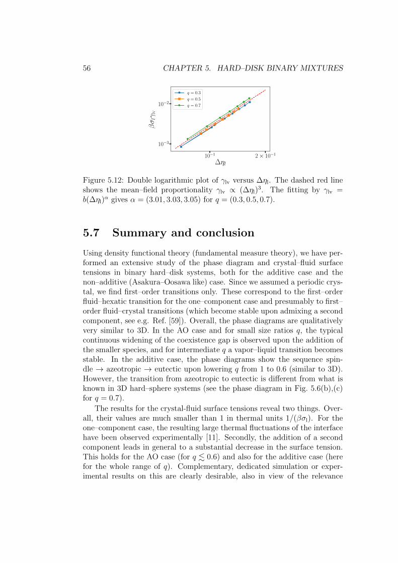
56 CHAPTER 5. HARD–DISK BINARY MIXTURES
10−1 2× 10⁻¹
∆ηl
10−3
10−2
βσlγ
lv
q = 0.3
q = 0.5
q = 0.7
Figure 5.12: Double logarithmic plot of γlv versus ∆ηl. The dashed red lineshows the mean–field proportionality γlv ∝ (∆ηl)
3. The fitting by γlv =b(∆ηl)
α gives α = (3.01, 3.03, 3.05) for q = (0.3, 0.5, 0.7).
5.7 Summary and conclusion
Using density functional theory (fundamental measure theory), we have per-formed an extensive study of the phase diagram and crystal–fluid surfacetensions in binary hard–disk systems, both for the additive case and thenon–additive (Asakura–Oosawa like) case. Since we assumed a periodic crys-tal, we find first–order transitions only. These correspond to the first–orderfluid–hexatic transition for the one–component case and presumably to first–order fluid–crystal transitions (which become stable upon admixing a secondcomponent, see e.g. Ref. [59]). Overall, the phase diagrams are qualitativelyvery similar to 3D. In the AO case and for small size ratios q, the typicalcontinuous widening of the coexistence gap is observed upon the addition ofthe smaller species, and for intermediate q a vapor–liquid transition becomesstable. In the additive case, the phase diagrams show the sequence spin-dle → azeotropic → eutectic upon lowering q from 1 to 0.6 (similar to 3D).However, the transition from azeotropic to eutectic is different from what isknown in 3D hard–sphere systems (see the phase diagram in Fig. 5.6(b),(c)for q = 0.7).
The results for the crystal-fluid surface tensions reveal two things. Over-all, their values are much smaller than 1 in thermal units 1/(βσl). For theone–component case, the resulting large thermal fluctuations of the interfacehave been observed experimentally [11]. Secondly, the addition of a secondcomponent leads in general to a substantial decrease in the surface tension.This holds for the AO case (for q . 0.6) and also for the additive case (herefor the whole range of q). Complementary, dedicated simulation or exper-imental results on this are clearly desirable, also in view of the relevance
5.7. SUMMARY AND CONCLUSION 57
of the surface tension for nucleation processes, see Ref. [63] for a review onmore qualitative results on 2D crystal and defect formation. The observeddecrease in surface tension should lead to a considerable decrease in the timescales of crystal nucleation.
In contrast to phase diagrams, results on crystal–fluid surface tensions inbinary 3D systems are scarce. For binary hard spheres with a size ratio ofq = 0.9, results are reported in Ref. [64]. For that q, the phase diagram isazeotropic. The surface tension is found to increase monotonically with theaddition of small spheres. These findings are similar to those for a 3D binaryLennard–Jones system with zero size mismatch, but a ratio of interactionstrengths of 0.75 (leading to a spindle–type phase diagram) [65], but theyare different from the non-monotonic behavior found here in the 2D system(see Fig. 5.11(a),(b)).
The full minimization of the FMT functionals show interesting effectsfor the density distributions in the crystal unit cells and of the crystal–fluidinterfaces. For intermediate size ratios (examples shown for q = 0.45) su-perpositions of substitutional and alloy structures are found, and enhancedcrystallinity and density of small disks is observed right at interface betweencrystal and fluid. Clearly, an extension of the present studies to the globalstability of alloy phases and their interfaces is desirable but requires consid-erable more efforts.


Chapter 6
Machine learning functional
Partial results of this chapter have been published in: SciPostPhys. 6, 025 (2019) with the title “A classical density functionalfrom machine learning and a convolutional neural network” [2]
With the steep increase of available computing power over the past years,methods of machine learning (ML) have come into the focus of research alsoin physics. ML is designed for finding patterns in high–dimensional data. Al-gorithms of ML still rely on insight and intuition how to represent and processdata, but a detailed model–building (specific for the problem at hand) is notrequired. The optimization of data representation/processing can be viewedas a numerically intensive data fitting task which is very familiar to physicists.Therefore it appears also natural to apply ML to the problem of functionalconstruction in DFT. In the past years, such ideas have been driven by thequantum DFT community. Refs. [16, 17] address the construction of a MLfunctional for the kinetic energy functional T [n] in one dimension (1D). Al-though successful in obtaining energy values, certain limitations when goingto three dimensions (3D) have led the authors of Ref. [18] to apply ML di-rectly to the functional map between the external potential and the electrondensity. Although the approach appears to be quite promising in terms ofpossible accuracy, it amounts to hiding the energy functional in a “ML blackbox”, which might appear less appealing to theorists.
Certainly, in the case of a “ML black box” functional one must be care-ful in choosing training data sets in relation to the applications one has inmind. For classical DFT, training data sets would be created most naturallyby Monte Carlo (MC) or Molecular Dynamics (MD) simulations. To keepnumerical efforts down, training sets should be created using small sets ofparameters (chemical potential, temperature, external potentials) with good
59
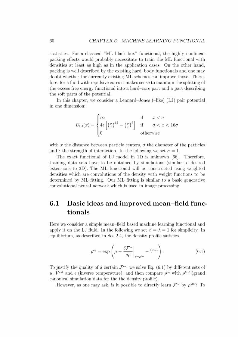
60 CHAPTER 6. MACHINE LEARNING FUNCTIONAL
statistics. For a classical “ML black box” functional, the highly nonlinearpacking effects would probably necessitate to train the ML functional withdensities at least as high as in the application cases. On the other hand,packing is well described by the existing hard–body functionals and one maydoubt whether the currently existing ML schemes can improve those. There-fore, for a fluid with repulsive cores it makes sense to maintain the splitting ofthe excess free energy functional into a hard–core part and a part describingthe soft parts of the potential.
In this chapter, we consider a Lennard–Jones (–like) (LJ) pair potentialin one dimension:
ULJ(x) =
∞ if x < σ
4ε[(
σx
)12 −(σx
)6]
if σ < x < 16σ
0 otherwise
with x the distance between particle centers, σ the diameter of the particlesand ε the strength of interaction. In the following we set σ = 1.
The exact functional of LJ model in 1D is unknown [66]. Therefore,training data sets have to be obtained by simulations (similar to desiredextensions to 3D). The ML functional will be constructed using weighteddensities which are convolutions of the density with weight functions to bedetermined by ML fitting. Our ML fitting is similar to a basic generativeconvolutional neural network which is used in image processing.
6.1 Basic ideas and improved mean–field func-
tionals
Here we consider a simple mean–field based machine learning functional andapply it on the LJ fluid. In the following we set β = λ = 1 for simplicity. Inequilibrium, as described in Sec.2.4, the density profile satisfies
ρeq = exp
(µ− δF ex
δρ
∣∣∣∣ρ=ρeq
− V ext
). (6.1)
To justify the quality of a certain F ex, we solve Eq. (6.1) by different sets ofµ, V ext and ε (inverse temperature), and then compare ρeq with ρMC (grandcanonical simulation data for the the density profile).
However, as one may ask, is it possible to directly learn F ex by ρMC? To

6.1. BASIC IDEAS AND IMPROVED MEAN–FIELD FUNCTIONALS61
facilitate such an idea, we define a ML output density as
ρML(x) = exp
(µ− δF ex,ML
δρ
∣∣∣∣ρ=ρMC
− V ext
), (6.2)
with ρMC the simulation result of equilibrium density profiles. To measurethe difference between ρMC and ρML, we define the loss function
L =M∑
k
∫(ρMC
k (x)− ρML
k (x))2 dx, (6.3)
where ρMCk is the k–th training sample (density distribution from simulation),
ρMLk is the corresponding ML output by Eq.(6.2), and M is number of training
sample. If we could give F ex,ML a certain ansatz, we should be able to find anapproximation of F ex,ML by minimizing L. The idea is actually very similarto a generative network, such as an autoencoder [67]. The ρMC/ρML is theinput/output, F ex,ML is an encoder, and Eq. (6.1) is a decoder.
But what form of F ex,ML should be used? In most cases, the excess freeenergy functional F ex of LJ is split into FHR and F att, such as F ex = FHR+F att
with FHR/F att denoting excess free energy functional from HR/attractivepotential, where F att is approximated by the mean–field (MF) approximation,
FMF =1
2
∫dx ρ(x)
∫dx′ ρ(x′)Uatt(|x− x′|). (6.4)
with
Uatt(x) =
0 if x < σ
ULJ(x) otherwise.
Analogously, we consider F ex,ML[ρ] = FHR + F ex,MLatt with
F ex,ML
att [ρ] = ε
∫dx ρ(x)n(x), (6.5)
and the weighted density n(x) =∫dx′ ρ(x′)ω(x− x′). The ω is the convolu-
tion kernel/weight function that needs to be trained. This is the weighted–density form of the RPA mean–field approximation in Eq. (6.4). Thus, thekernel ω should somehow correspond to Uatt/(2ε). To minimize L, we usethe gradient decent [68], where ω is updated by 1
ωnew(x) = ωold(x)− α∂L∂ω
∣∣∣∣ω=ωold
(6.6)
1rigorously speaking, since L is a functional of ω, it should be δLδω .

62 CHAPTER 6. MACHINE LEARNING FUNCTIONAL
with α the learning rate. The gradient descent is based on Taylor expansionas L(ω+ ε) ' L(ω) + ε∂L
∂ωfor small ε. If one sets ε = −α∂L
∂ω, then L(ω+ ε) '
L(ω)−α(∂L∂ω
)2< L(ω) for a small and positive α. As one can see, the gradient
descent stops when ∂L∂ω
= 0, so it will find a local minimum. Furthermore,the term ∂L
∂ωwith the symmetry assumption ω(x) = ω(−x) can be written as
∂L
∂ω (x′)= −4
∑
k
∫dx (ρMC
k (x)− ρML
k (x)) ρML
k (x) εkρMC
k (x+ x′)
. (6.7)
For a more complex ansatz (see next section), this term will be too cumber-some to determine by hand. Fortunately in the modern ML programmingtools, such as Tensorflow[69] and PyTorch[70], it is automatically handledby back–propagation. For the details of machine learning, we refer to Ref [68]as an overview, for interested readers.
6.2 Result and conclusion
To train ω, we prepare 1115 density profiles by grand canonical simulation.The V ext is a hard–wall slit of width 32 σ with 3 additional Gaussian poten-tials of random strength/width and location inside the slit (see Fig. 6.1a); εand µ are randomly in the range of 0.5...1.5 and ln 0.5... ln 2.0.
In Fig. 6.1, we shows the final result of the kernel ω after training andthe loss functional (Eq. (6.3)) versus iterations. The tail of ω is close toUatt/(2ε) as expected, and it extends somewhat into the hard–core region.Furthermore we show the pressure versus the bulk density (equation of state,eos), and the density profile on a hard wall in Fig. 6.2.
As shown in Fig. 6.2, the results by F ex,ML is better then the naive mean–field approximation. The contribution to F ex[ρ] from attractive interactionsoutside the hard core is treated by mean–field concepts in various guises [27,71, 72, 73, 74]. With the F ex,ML introduced in this section, we obtain ω andthus F ex directly from ρMC. However, even with the improvement, it is stilla mean–field type functional. Due to the simple ansatz, the improvement isunsatisfactory; moreover, not all particle–particle potentials may allow forthe splitting into a well–understood reference part and a remainder to belearned by ML, such as FHR in this case. In the next chapter, we introducea more flexible ML architecture, which is capable of giving F ex,ML beyondmean–field type functional and even forego FHR.

6.2. RESULT AND CONCLUSION 63
0 5 10 15 20 25 30
x/σ
0.0
0.1
0.2
0.3
0.4
0.5
ρσ
−2
−1
0
1
2
Vext
∞ ∞
ρMC
V ext
(a)
100 101 102 103 104 105
number if iterations
10−2
10−1
L
(b)
−4 −2 0 2 4
x/σ
−0.4
−0.2
0.0
ω(x)
MLMF
(c)
Figure 6.1: (a) An example of V ext and ρMC with µ = ln(1.40) and ε = 1.24,(b) loss versus iterations, and (c) RPA–like mean–field approximation. In(a), the black solid line is ρMC corresponding to the left y–axis and bluedashed line is V ext corresponding to the right y–axis. In (c), the black solidline is the ML–optimized ω(x), and for comparison Uatt(x)/(2ε) is shown bythe blue dashed line.
0.0 0.1 0.2 0.3 0.4 0.5 0.6
ρσ
0.0
0.2
0.4
0.6
0.8
1.0
Pσ
MC, ǫ =1.0MLMFMC, ǫ =2.0MLMFMC, ǫ =3.0MLMF
(a)
1 3 5
x/σ
0.0
0.5
1.0
1.5
ρσ
MLMFMC
(b)
Figure 6.2: (a) equation of sate, and (b) ρ(x) on a hard–wall potential forε = 1.5 and µ = ln 1.5. The ML and MF density profiles are obtained byiteratively solving Eq. (6.1) with the density profiles initialized by a constantvalue.


Chapter 7
Functional equation learner
Partial results of this chapter have been published in: J. Chem.Phys. 152, 021102 (2020) with the title “Analytical classical den-sity functionals from an equation learning network”[75]
In Chapter 6, we introduce a mean–field–like machine learning (ML) func-tional. Despite the improvement comparing to the naive mean–field approx-imation, the form of the functional is limited.
From a thoery point of view, the excess functionals derived from Funda-mental Measure Theory (FMT) [8] have a high degree of accuracy [3, 8, 34]for hard spheres and hard anisotropic particles [76, 77, 78]. However, thecontribution to F ex[ρ] from attractive interactions outside the hard core istreated by mean–field concepts in various guises (random phase approxima-tion (RPA) [71], functional expansions [27, 72], Wertheim theory for patchyattractions [73, 74] etc.) but a qualitatively new and successful ansatz, suchas FMT hard–body–treatment, is missing.
Thus, to extend the flexibility of the ML functional and success of FMT,the network we propose, Functional Equation Learner (FEQL), is an L–layered feed–forward network with computational units specifically designedfor constructing the free energy functional (see Fig. 7.1).
The first layer consists of convolution kernels which compute the weighteddensities ni with the convolution kernel ωi (i = 1...nw) by
ni(x) = ρ⊗ ωi =
∫dx′ ρ(x′)ωi(x− x′) , (7.1)
and some of the weighted densities are multiplied by ε in the case of the LJfluid. Using weighted densities instead of the particle density is inspired bythe exact HR functional [34] and fundamental measure theory [4, 8]. The
65
66 CHAPTER 7. FUNCTIONAL EQUATION LEARNER
layer 2 is a linear, all–to–all mapping of the vector (of functions) n = ni(x)to the vector
z(l=1) = W (1)n (7.2)
at level l = 1. The layers 3...L − 4 are a sequence of nonlinear and lineartransformations.
The non-linear transformation at level l contains u unary units fI and vbinary units gJ and maps z(l)(x) (u + 2v–dimensional) to the layer outputy(l) (u+ v–dimensional) as:
y(l) :=(f1
(z
(l)1
), f2
(z
(l)2
)...fu
(z(l)u
),
g1
(z
(l)u+1, z
(l)u+2
)...gv
(z
(l)u+2v−1, z
(l)u+2v
)). (7.3)
The unary units, f1, ..., fu receive the respective component, z1, ..., zu asinputs, and each unit is one of the following base functions indexed byI ∈ 0, 1, 2:
fI(zi) :=
zi if I = 0
exp(zi)− 1 if I = 1
ln(zi + 1) if I = 2
The binary units, g1, ..., gv receive the remaining component, zu+1, ..., zu+2v,as input in pairs of two, and each unit may be multiplication or divisionindexed by J ∈ 0, 1:
gJ(zi, zi+1) :=
zi × zi+1 if J = 0
zi ÷ (zi+1 + 1) if J = 1
Note that fI(0) = gJ(0, z) = 0. One may worry about divergences in divisionand logarithm when z → −1. In the beginning of the training procedure,all parameters and convolution kernel are initialized by small numbers andthus z, fI and gJ are close to zero. If z is too close to -1, the loss will changedrastically; thus the network will intrinsically handle this issue. As mentionedin Ref. [22], one could use modified division and logarithm functions and addextra penalties. However, it turns out not to be required here.
The linear transformation from level l to l+1 maps the (u+v)–dimensionalinput y(l) to the (u+2v)–dimensional intermediate representation z(l+1) givenby
z(l+1) = W (l+1)y(l). (7.4)
Thus, the nw convolution kernels ω(x) in the first layer and the matrices W (l)
are free parameters that are learned during training.
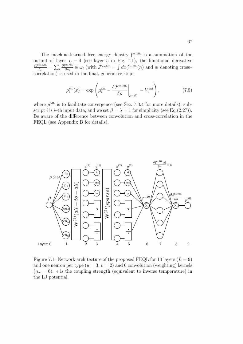
67
The machine-learned free energy density fex,ML is a summation of theoutput of layer L − 4 (see layer 5 in Fig. 7.1), the functional derivativeδFex,ML
δρ=∑
i∂fex,ML
∂ni⊕ ωi (with F ex,ML =
∫dx fex,ML(n) and ⊕ denoting cross–
correlation) is used in the final, generative step:
ρML
i (x) = exp
(µML
i −δF ex,ML
δρ
∣∣∣∣ρ=ρeq
i
− V exti
), (7.5)
where µMLi is to facilitate convergence (see Sec. 7.3.4 for more details), sub-
script i is i–th input data, and we set β = λ = 1 for simplicity (see Eq.(2.27)).Be aware of the difference between convolution and cross-correlation in theFEQL (see Appendix B for details).
Figure 7.1: Network architecture of the proposed FEQL for 10 layers (L = 9)and one neuron per type (u = 3, v = 2) and 6 convolution (weighting) kernels(nw = 6). ε is the coupling strength (equivalent to inverse temperature) inthe LJ potential.

68 CHAPTER 7. FUNCTIONAL EQUATION LEARNER
7.1 Physical constraints
Since F ex,ML approximates F ex, we must consider two physical constraints:
(i) F ex,ML(ρ = 0) = 0 and (ii) δFex,ML
δρ
∣∣∣ρ=0
= 0. To enforce (i), we choose
the linear mapping without bias and f(0) = g(0, z) = 0 in the non–linearmapping. Condition (ii) can be enforced by setting appropriate parametersin the matrix W (l) of the final level to zero. This requires to determine the
analytic form of ∂fex,ML
∂ni
∣∣∣ρ=0
to identity those parameters. For example, for a
FEQL with nw = 2, 2 levels and (1,0,0,1,0) node for (identity, exponential,logarithm, multiplication and division),
fex,ML =a2L0(a1L0n0 + a1L1n1) + a2L1(a1L2n0 + a1L3n1)(a1L4n0 + a1L5n1)+
(a2L2(a1L0n0 + a1L1n1) + a2L3(a1L2n0 + a1L3n1)(a1L4n0 + a1L5n1))
(a2L4(a1L0n0 + a1L1n1) + a2L5(a1L2n0 + a1L3n1)(a1L4n0 + a1L5n1))(7.6)
with axLy the y–th parameter in W (x). Then we calculate ∂fex,ML
∂ni
∣∣∣ρ=0
, such
as ∂fex,ML
∂n0
∣∣∣∣ρ=0
= a1L0 a2L0, and ∂fex,ML
∂n1
∣∣∣∣ρ=0
= a1L1 a2L0. Thus we set a2L0 = 0
in order to keep δFex,ML
δρ
∣∣∣ρ=0
= 0; this is the reason in Fig. 7.1 the W (2) is
labeled as sparse.
7.2 Network training
To obtain training data for ρeq, grand canonical simulations are used in thecase of LJ fluid; for the HR fluid, Eq. (2.27) is directly solved, since the exactfunctional is known.
FEQL is fully differentiable in its free parameters θ = [W,ω] and can thusbe trained using back–propagation. We adopt the following loss function
L =1
N
N∑
i=1
(α1
∫|ρeq
i − ρML
i | d x+ α2|µeq
i − µML
i |)
+λ1
∑
i
∫dx |ωi|+ λ2
∑
l,βγ
|W (l)βγ |, (7.7)
with α1 = 0.9 and α2 = 0.1. These values have been determined empiricallyand the exact choice is not critical. For training we choose Adam [79] with

7.3. RESULTS 69
mini-batches:
θt+1 = θt + Adam
(∂L (D (t))
∂θ, α
)(7.8)
with α the stepsize parameter (learning rate) and D(t) the data in the cur-rent mini-batch. The choice of Adam is not critical and standard stochasticgradient descent also accomplished the task.
Following Sahoo et al. [22], we adopt a three–step training procedure. Atthe beginning, we use no regularization (λ1 = λ2 = 0), such that parameterscan vary freely and reach reasonable starting points. In step 2, we switch onthe regularization by setting λ1 and λ2 to positive finite values to sparsifythe network for obtaining a simpler functional. In step 3, we clamp smallparameters with |W (l)
βγ | < wth to zero. In this way we keep the sparsity intro-duced by the lasso [80] training in step 2, but make sure unbiased parametervalues are attained. In this paper we choose α = 10−2 or 10−3, λ1 = 10−7
and wth = 0.05.
7.3 Results
To exam the ability of FEQL, we investigate the HR pair potential:
UHR(x) =
∞ if x < σ
0 otherwise
as well as the LJ(–like) potential:
ULJ(x) =
∞ if x < σ
4ε[(
σx
)12 −(σx
)6]
if σ < x < 16σ
0 otherwise
in one dimension with x the distance between particle centers, σ the diameterof the particles and ε the strength of interaction. In the following we setσ = 1.
7.3.1 Hard rods
The hard–rod (HR) fluid is one of a few systems that F ex is exactly known.The exact equation of state (eos) is given by the pressure P (ρ) = ρ
1−ρ and
the exact analytic form of FHR (Percus functional) is described in Sec. 3.3.3.The parameter of F ex,ML are trained using 1024 density profiles in a hard
wall slit of width 32 σ with 3 additional Gaussian potentials of random
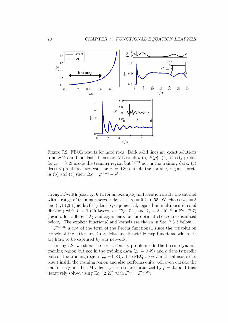
70 CHAPTER 7. FUNCTIONAL EQUATION LEARNER
0.0 0.2 0.4 0.6 0.8
ρσ
0
2
4
6
8Pσ
training
exactML
0
2
Vex
t
∞
0 5 10 15 20 25 30
x/σ
0.0
0.5
1.0
ρσ 0 30
-0.010
0.01
∆ρσ
0 2 4 6 8 10
x/σ
0
1
2
3
4
ρσ
0 5 10-0.2
0
0.2
0.4
∆ρσ
Figure 7.2: FEQL results for hard rods. Dark solid lines are exact solutionsfrom FHR and blue dashed lines are ML results. (a) P (ρ). (b) density profilefor ρ0 = 0.49 inside the training region but V ext not in the training data. (c)density profile at hard wall for ρ0 = 0.80 outside the training region. Insetsin (b) and (c) show ∆ρ = ρexact − ρML.
strength/width (see Fig. 6.1a for an example) and location inside the slit andwith a range of training reservoir densities ρ0 = 0.2...0.55. We choose nw = 3and (1,1,1,3,1) nodes for (identity, exponential, logarithm, multiplication anddivision) with L = 9 (10 layers, see Fig. 7.1) and λ2 = 8 · 10−5 in Eq. (7.7)(results for different λ2 and arguments for an optimal choice are discussedbelow). The explicit functional and kernels are shown in Sec. 7.3.3 below.
F ex,ML is not of the form of the Percus functional, since the convolutionkernels of the latter are Dirac delta and Heaviside step functions, which areare hard to be captured by our network.
In Fig.7.2, we show the eos, a density profile inside the thermodynamictraining region but not in the training data (ρ0 = 0.49) and a density profileoutside the training region (ρ0 = 0.80). The FEQL recovers the almost exactresult inside the training region and also performs quite well even outside thetraining region. The ML density profiles are initialized by ρ = 0.5 and theniteratively solved using Eq. (2.27) with F ex = F ex,ML.

7.3. RESULTS 71
The virial expansion
PML(ρ) ' ρ+ 1.03ρ2 + 0.71ρ3 +O(ρ4)
(7.9)
of the ML eos shows moderate deviations compared to the exact one ( ρ1−ρ =
ρ+ ρ2 + ρ3...).One sees that inaccuracies in these coefficients do not necessarily lead
to a poor eos. Despite inaccurate coefficients, the higher order terms inthe learned eos combine appropriately to give a good representation of theexact eos. This is understandable since no explicit information about virialcoefficients is incorporated into the loss function, thus the learning procedurehas little incentive to find the correct coefficients.
Optimization for hard rod
0 1000 2000 3000 4000 5000 6000 7000
number of iterations
10−3
10−2
10−1
L
step 1 step 2 step 3λ2 = 10−2
λ2 = 10−3
λ2 = 10−4
λ2 = 10−5
Figure 7.3: Loss as a function of number of iterations for 4 different valuesof λ2. Dashed lines are validation loss and solid circles are training loss.
In Eq. (7.7), the third term with coefficient λ2 is used as a substitute forthe number of nonzero entries in the matrices W (l), which is not differentiabledirectly. Nevertheless, minimizing the absolute norm tends to produce sparsesolutions, see also Lasso regression [80], and thus favors simpler functionals.Before training, we prepared 1024 density profiles with a range of reservoirdensities ρ0 = 0.2...0.55, and randomly divided them into 921 density profilesas the training set and 103 as the validating set. The training procedure onlyuses the training set for updating trainable parameters and evaluates thevalue of the loss on the training set and on the validating set (called trainingloss and validation loss) at the end of each iteration [68]. Additionally, we also

72 CHAPTER 7. FUNCTIONAL EQUATION LEARNER
prepare 256 density profiles with a range of reservoir densities ρ0 = 0.6...0.8,outside the training region, as a measurement for extrapolative capabilities.
Then, as described in before (Sec. 7.2), we have used a three–step trainingprocedure. In Fig. 7.3 we show the evolution of the training and validationloss throughout the training for 4 different values of λ2. For the higher valuesof λ2 (10−2 and 10−3) there is a marked increase of L at the beginning ofstep 2. For λ = 10−4 the beginning of step 2 is not marked with an increaseof L and then L further decreases.
10−810−710−610−510−410−310−2
λ2
10−3
10−2
L
validationtrainingextrapolation
(a) Final loss versus λ2.
10−810−710−610−510−410−310−2
λ2
01020304050607080
com
plex
ity
(b) complexity versus λ2.
0 10 20 30 40 50 60 70 80
complexity
10−3
10−2
L
validationtrainingextrapolation
(c) complexity versus loss.
Figure 7.4: The interdependence of loss, complexity and λ2.
This is further confirmed in Fig. 7.4a, which shows the final value of Lfrom the training, validating, and extrapolating set as a function of λ2. Theloss shows underfitting for λ2 > 10−3 and overfitting for λ2 < 10−7. Near–optimal choices are 10−6 < λ2 < 10−4. The complexities (the number ofnonzero entries in W ) increase with decreasing of λ2 (Fig. 7.4b). For a broadrange of complexities, the loss is almost constant (Fig. 7.4c).
7.3.2 Lennard–Jones
Here, 1115 training distributions are generated with random ε and µ in therange of 0.5...1.5 and ln 0.5... ln 2, respectively, with V ext prescribed as in thehard–rod case (see Fig. 6.1a for an example). The training data are obtainedby grand canonical Monte Carlo (GCMC) simulation.
Splitting between repulsions and attractions
Following liquid state theory [2] and similar in spirit to Chap. 6, we split F ex
into a contribution from repulsions and one from attractions as follows:
F ex,ML([ρ]; ε) = FHR([ρ]) + εF ex,ML
att ([ρ]; ε), (7.10)
where the factor ε in front of the F ex,MLatt makes sure F ex,ML(ε→ 0) = FHR, and
F ex,MLatt is to be learned by the network. In Fig. 7.1, the output from the layer

7.3. RESULTS 73
6 is F ex,MLatt ; we multiply the output from the layer 8 by ε, add contribution
from FHR, and then feed it to layer 9. In the first layer, we choose nw = 4, 1kernel multiplied by ε and another 3 without this factor (see Fig. 7.1), and(1,1,1,2,1) nodes for (identity, exponential, logarithm, multiplication and di-vision). The training parameter λ2 = 5 ·10−5 in Eq. (7.7). Results are shownbelow in Fig. 7.5. The explicit functional and kernels are shown in Sec. 7.3.3.The findings are similar to the HR case with a very good match to simulationdata for the eos and test distributions inside and outside the thermodynamictraining region. For a 1D system with hard–core repulsive and finite–rangedattractive pair potential, the pressure must be monotonically increasing forarbitrary low temperature (high ε), and thus there is no gas–liquid transi-tion [81]. The corresponding ML pressure shows no van der Waals (vdW)loop for attractions strengths up to ε = 4.1.
0.0 0.2 0.4 0.6 0.8
ρσ
0
1
2
3
4
5
6
Pσ
MC, ǫ =1.0MLMC, ǫ =1.5MLMC, ǫ =3.0MLMC, ǫ =4.5ML
02
Vex
t ∞
0 2 4 6 8 10 12 14
x/σ
0.0
0.4
0.8
1.2
ρσ
MCML
0 8-0.02
0
0.02∆ρσ
2 4 6 8 10
x/σ
0
1
2
ρσ 0 5 10
-0.2
-0.1
0.0
∆ρσ
Figure 7.5: FEQL results for LJ fluid with functional splitting. (a) eos P (ρ).(b) density profile for ε = 1.30, µ = ln(1.27) inside the training region butV ext not in the training data. (c) density profile at a hard wall for ε = 1.7,µ = ln(1.7), outside the training region. Dark solid lines are simulationprofiles and blue dashed lines are ML results. Insets in (b) and (c) show∆ρ = ρMC − ρML.
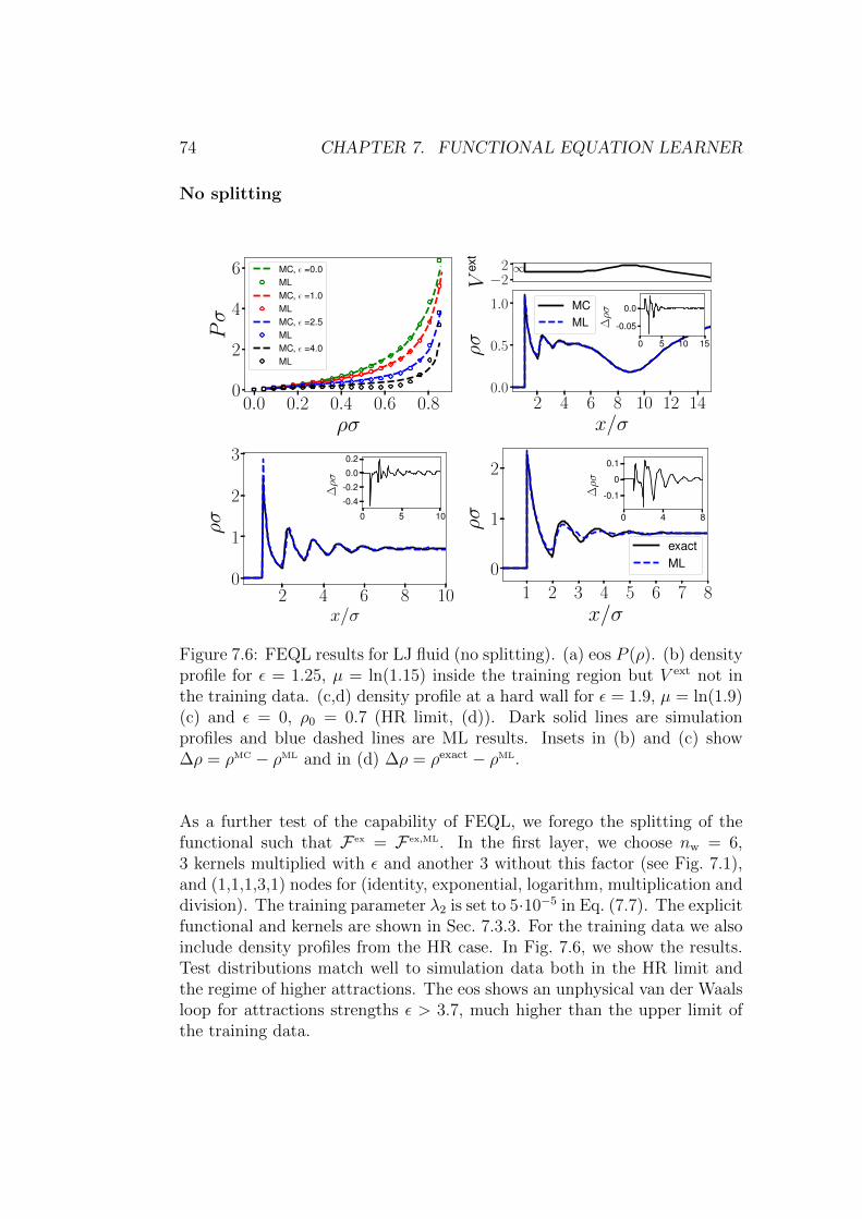
74 CHAPTER 7. FUNCTIONAL EQUATION LEARNER
No splitting
0.0 0.2 0.4 0.6 0.8ρσ
0
2
4
6
Pσ
MC, ǫ =0.0MLMC, ǫ =1.0MLMC, ǫ =2.5MLMC, ǫ =4.0ML
−22
Vex
t
∞
2 4 6 8 10 12 14x/σ
0.0
0.5
1.0
ρσ
MCML
0 5 10 15
-0.05
0.0
∆ρσ
2 4 6 8 10x/σ
0
1
2
3
ρσ 0 5 10
-0.4
-0.2
0.0
0.2
∆ρσ
1 2 3 4 5 6 7 8x/σ
0
1
2ρσ
exactML
0 4 8
-0.1
0
0.1
∆ρσ
Figure 7.6: FEQL results for LJ fluid (no splitting). (a) eos P (ρ). (b) densityprofile for ε = 1.25, µ = ln(1.15) inside the training region but V ext not inthe training data. (c,d) density profile at a hard wall for ε = 1.9, µ = ln(1.9)(c) and ε = 0, ρ0 = 0.7 (HR limit, (d)). Dark solid lines are simulationprofiles and blue dashed lines are ML results. Insets in (b) and (c) show∆ρ = ρMC − ρML and in (d) ∆ρ = ρexact − ρML.
As a further test of the capability of FEQL, we forego the splitting of thefunctional such that F ex = F ex,ML. In the first layer, we choose nw = 6,3 kernels multiplied with ε and another 3 without this factor (see Fig. 7.1),and (1,1,1,3,1) nodes for (identity, exponential, logarithm, multiplication anddivision). The training parameter λ2 is set to 5·10−5 in Eq. (7.7). The explicitfunctional and kernels are shown in Sec. 7.3.3. For the training data we alsoinclude density profiles from the HR case. In Fig. 7.6, we show the results.Test distributions match well to simulation data both in the HR limit andthe regime of higher attractions. The eos shows an unphysical van der Waalsloop for attractions strengths ε > 3.7, much higher than the upper limit ofthe training data.

7.3. RESULTS 75
7.3.3 Explicit functional and convolution kernels
Here we show the full functional of F ex,ML[n], with
ni(x) =
∫dx′ ρ(x′)ωi(x− x′). (7.11)
The coefficients in F ex,ML are single precision; for displaying purposes, allcoefficients are rounded to the one decimal place and then rationalized.
F ex,ML for hard rod
The FEQL result for hard rod in Sec. 7.3.1 is
Fex,ML =
∫dx
n20
5+ n0
10y0 − n2
210
−n20
5− n0
5y0 − n0
10+ ey1
5+ 4
5
+ y2
(−n
20
5− n0
10y0 −
3
10ey1 +
3
10
)+ ey3 − 1 (7.12)
with y0 = 2n0
5+ n2
5, y1 = 3n1
5, y2 = 2n0
5− n1
5+
n22
10− n2
10, y3 =
n20
10and convolution
kernels ωi shown in Fig.7.7a.
F ex,ML for LJ with splitting
In Sec. 7.3.2 with splitting, F ex = FHR + εF ex,MLatt , where
Fex,MLatt =
∫dx
3
5y0y1
(− εn3
2− n0
10− n1
10− n2
2+y0y1
5− y2y3
5− 2y4
5y5
)− y0y1
10− y2y3
5
− y2y3
10
(εn35
+ n25− 7y0y1
10+ 3y2y3
5− 2 ln y6
5+ 1− −εn3−
n02−n1
10− 11n2
1010y5
)+
(3εn3
10+n0
10+
3n2
10− y0y1
2+
9y2y3
10+
ln y6
10+−εn3 − n0
2− n1
10− 11n2
10
10y5
)(−3εn3
10− n0
10− n1
10− 2n2
5+
3y0y1
10− 3y2y3
10+ey7
5− 1
5− 9y4
10y5
)+ e−
2y0y15− y2y3
5 + ln(−y2y3
5+ 1)− 1
(7.13)
with
y0 =n0
5− 2n1
5+n2
10, y1 =
εn3
2− 3n0
10− 2n1
5+
3n2
10, y2 =
εn3
10+n0
5− 3n1
10− 2n2
5, y3 =
εn3
10+n0
5+n1
5− 3n2
10,
y4 = −εn3 −n0
2− n1
10− 11n2
10, y5 = −2εn3
5− 6n1
5+ 1, y6 = −3εn3
10+n2
10+ 1, y7 = − εn3
5+
2n0
5
and convolution kernels ωi shown in Fig.7.7b

76 CHAPTER 7. FUNCTIONAL EQUATION LEARNER
F ex,ML for LJ without splitting
The result of F ex given by FEQL in Sec. 7.3.2 without splitting is
Fex,ML =
∫dx
y0 ln y1
10+y2y3
10+− y4y5
2+ 3y2y3
10− y6y7
23y4y5
10+ 3 ln y1
10+ 1
+
(−y4y5
5+
17ey8
10+
4 ln y1
5− 17
10
)(−3εn3
5− n0
10+n2
5+y2y3
2− 9 ln y1
5
)+
(− εn3
5+n2
10+
3y4y5
10+−n0
10− n1
5+ n2
10
5y9+y6y7
5
)(− εn3
5+n2
10+
2y4y5
5+−n0
10− n1
5+ n2
10
5y9+y6y7
5+ey8
10− 1
10
)
+ ey2y3
5− 3y6y7
10 + ln(y2y3
10+ 1)− 1 (7.14)
with
y0 = − εn3
5+n2
10, y1 = −7n1
10− 7n2
10+ 1, y2 =
3εn5
10− 2n0
5+n2
10, y3 =
2εn4
5− 2εn5
5− n1
10− n2
10,
y4 = −3n0
10− n1
2+
3n2
10, y5 =
2n0
5+
2n1
5− 3n2
10, y6 = − εn5
5− 3n0
10− 2n1
5+
3n2
10,
y7 =εn5
2+n0
10+
2n1
5− n2
5, y8 =
n0
10− 3n1
10− 3n2
5, y9 = −3n0
10− n1
2+n2
10+ 1
and convolution kernels ωi shown in Fig.7.7c
−4 −3 −2 −1 0 1 2 3 4
x/σ
−4
−2
0
2
ω
ω0
ω1
ω2
ωexact0
ωexact1
(a)
−8 −6 −4 −2 0 2 4 6 8
x/σ
−2
−1
0
1
2
ω ω0
ω1
ω2
ω3
(b)
−8 −6 −4 −2 0 2 4 6 8
x/σ
−1.5
−0.5
0.5
1.5
ω
ω0
ω1
ω2
ω3
ω4
ω5
(c)
Figure 7.7: ω for all cases. (a)HR. The ωexacti are the exact weight kernels
in Eqs. (3.55). (b)LJ, splitting (c)LJ, no splitting. The maximum allowedrange for the kernels is [−4σ, 4σ] in the HR case and [−8σ, 8σ] in the LJ case.

7.3. RESULTS 77
7.3.4 Consistency of µ
In Eq. (7.5), µMLi is determined by demanding that
∫(ρMLi − ρeq
i )2 is mini-mal, which entails that µML
i varies during the iterations. This choice of µMLi
stabilizes the training process, and µMLi is directly determined by
∂
∂µMLi
∫(ρML
i − ρeq
i )2 = 0⇒ µML
i = ln
(∫ρeq
i ρ′MLi∫
(ρ′MLi )2
), (7.15)
where ρ′MLi = exp
(− δFex,ML
δρ
∣∣∣∣ρ=ρeq
i
− V exti
). If the training converges, µML
will converge to µeq. In Fig.7.8 we show ∆µ = µeq−µML versus µeq at the endof training for the three cases in Sec. 7.3.1 and 7.3.2. µML is indeed close toµeq.
−0.75 −0.25 0.25 0.75 1.25
βµeq
−0.01
0.00
0.01
β∆µ
TrainingValidation
(a)
−0.6−0.4−0.2 0.0 0.2 0.4 0.6
βµeq
−0.01
0.00
0.01
0.02
β∆µ
(b)
−0.75 −0.25 0.25 0.75 1.25
βµeq
−0.04
−0.02
0.00
0.02
0.04
β∆µ
(c)
Figure 7.8: ∆µ = µeq − µML versus µeq. (a) HR (b) LJ with splitting (c) LJ,no splitting.

78 CHAPTER 7. FUNCTIONAL EQUATION LEARNER
Furthermore, we also check µ(ρ) = ∂f∂ρ
(i.e. from the equation of state),
where ρ here refers to the density of the bulk fluid. In Fig. 7.9 we show µ(ρ)from the exact functional, ML, and MC simulations for the three cases as inthe Sec. 7.3.1 and 7.3.2. Deviations only occur for the LJ case well outsidethe training region.
In principle, one could also fix µMLi = µeq
i (the chemical potential of thedata set) and then choose α1 = 1 and α2 = 0 in Eq. (7.7), but this requiressmaller learning rates and results in much longer training processes. Forexample, the HR case with parameters as in the main paper can be donewith learning rate = 10−3 and the number of training iterations doubled.
0.0 0.2 0.4 0.6 0.8
ρσ
−4
0
4
8
12
βµ training
exactML
(a)
0.0 0.2 0.4 0.6 0.8ρσ
−4
−2
0
2
4βµ
ǫ =1.0ǫ =1.5ǫ =3.0ǫ =4.5
(b)
0.0 0.2 0.4 0.6 0.8ρσ
−4
−2
0
2
4
βµ
ǫ =0.0ǫ =1.0ǫ =2.5ǫ =4.0
(c)
Figure 7.9: µ(ρ) versus ρ. (a) HR (b) LJ with splitting (c) LJ, no splitting.In (b) and (c), the circles are ML and dashed lines are MC simulations.
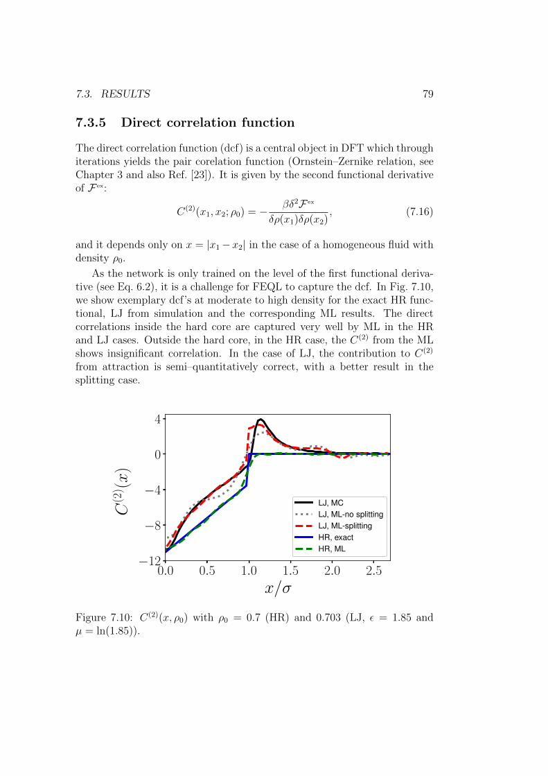
7.3. RESULTS 79
7.3.5 Direct correlation function
The direct correlation function (dcf) is a central object in DFT which throughiterations yields the pair corelation function (Ornstein–Zernike relation, seeChapter 3 and also Ref. [23]). It is given by the second functional derivativeof F ex:
C(2)(x1, x2; ρ0) = − βδ2F ex
δρ(x1)δρ(x2), (7.16)
and it depends only on x = |x1−x2| in the case of a homogeneous fluid withdensity ρ0.
As the network is only trained on the level of the first functional deriva-tive (see Eq. 6.2), it is a challenge for FEQL to capture the dcf. In Fig. 7.10,we show exemplary dcf’s at moderate to high density for the exact HR func-tional, LJ from simulation and the corresponding ML results. The directcorrelations inside the hard core are captured very well by ML in the HRand LJ cases. Outside the hard core, in the HR case, the C(2) from the MLshows insignificant correlation. In the case of LJ, the contribution to C(2)
from attraction is semi–quantitatively correct, with a better result in thesplitting case.
0.0 0.5 1.0 1.5 2.0 2.5
x/σ
−12
−8
−4
0
4
C(2) (x)
LJ, MCLJ, ML-no splittingLJ, ML-splittingHR, exactHR, ML
Figure 7.10: C(2)(x, ρ0) with ρ0 = 0.7 (HR) and 0.703 (LJ, ε = 1.85 andµ = ln(1.85)).

80 CHAPTER 7. FUNCTIONAL EQUATION LEARNER
7.3.6 Learning the exact HR functional
Figure 7.11: Simplified FEQL for hard–rod functional
As shown in Sec. 7.3.1, even though the learned functional for hard–rod fluidsbehaves well inside and outside the training region, it is not in the form of thePercus functional (Eq. (3.55)). This is understandable, since the convolutionkernels of the latter are Dirac delta and Heaviside step functions, which arehard to be captured by our network. Also, the possible configuration oftrained functionals, i.e, local minima, are too many such that the chance forFEQL to find the global minimum (the Percus functional) is scarce. To showthat the FEQL is capable of delivering the “correct” functional, we limitnw = 2 and keep only the necessary nodes as shown in Fig. 7.11; thus thethe untrained functional is
F ex,ML =
∫dx (a2L0 (a1L0n0 + a1L1n1) + a2L1 ln (a1L2n0 + a1L3n1 + 1))×
(a2L3 (a1L0n0 + a1L1n1) + a2L4 ln (a1L2n0 + a1L3n1 + 1))(7.17)
with axLy the y–th trainable parameter in W (x).We use 2048 density profiles as mentioned in Sec. 7.3.1 with a range
of training reservoir densities ρ0 = 0.2...0.8 for training, and add an extrapenalty term
∑
i
∫ L
0
∣∣∣∣(
tanh
(x− dw
)− tanh
(x− L+ d
w
))ωi(x)
∣∣∣∣dx (7.18)
with d = 1σ, w = 0.1σ and L system size (32σ), into the cost function(Eq. (7.7)). Fig. 7.12 shows the tanh term in Eq. (7.18); this extra regular-ization strongly localizes ω’s within ±1σ (with periodic boundary condition).
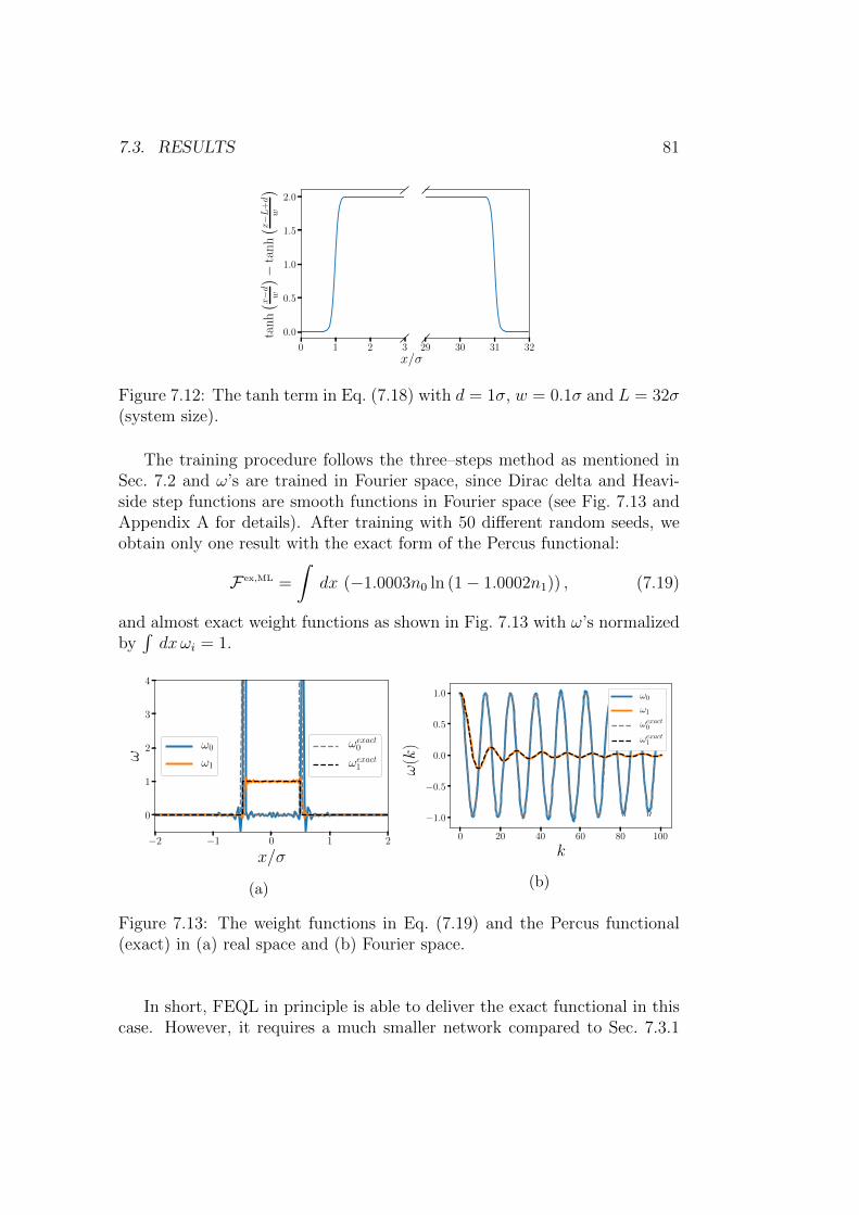
7.3. RESULTS 81
0 1 2 3
0.0
0.5
1.0
1.5
2.0
tanh( x
−d w
) −tanh( x
−L+d
w
)
29 30 31 32x/σ
Figure 7.12: The tanh term in Eq. (7.18) with d = 1σ, w = 0.1σ and L = 32σ(system size).
The training procedure follows the three–steps method as mentioned inSec. 7.2 and ω’s are trained in Fourier space, since Dirac delta and Heavi-side step functions are smooth functions in Fourier space (see Fig. 7.13 andAppendix A for details). After training with 50 different random seeds, weobtain only one result with the exact form of the Percus functional:
F ex,ML =
∫dx (−1.0003n0 ln (1− 1.0002n1)) , (7.19)
and almost exact weight functions as shown in Fig. 7.13 with ω’s normalizedby∫dxωi = 1.
−2 −1 0 1 2
x/σ
0
1
2
3
4
ω
ω0
ω1
ωexact0
ωexact1
(a)
0 20 40 60 80 100
k
−1.0
−0.5
0.0
0.5
1.0
ω(k)
ω0
ω1
ωexact0
ωexact1
(b)
Figure 7.13: The weight functions in Eq. (7.19) and the Percus functional(exact) in (a) real space and (b) Fourier space.
In short, FEQL in principle is able to deliver the exact functional in thiscase. However, it requires a much smaller network compared to Sec. 7.3.1

82 CHAPTER 7. FUNCTIONAL EQUATION LEARNER
and an extra regularization. Also the result is sensitive to the initial guessesof axLy’s in Eq. (7.17), which is probably due the size of the network. Itsrestricted form is in contradiction to having a “flexible” network as used inthe previous sections. Nevertheless, here we only attempt to demonstratethat it is possible to obtain the exact functional from FEQL.
7.4 Conclusion
The adaptation of EQL [22] to the classical DFT problem of finding F ex hasshown satisfactory results for the exemplary cases of the 1D HR and LJ fluid.The new network FEQL is very flexible and goes significantly beyond thepolynomial ansatz used in Ref. [2]. The analytic form allows for more easilytransferable output and further calculations to obtain, e.g., direct correlationfunctions. Also, for the HR case, it is possible to deliver the exact functionalwhile it requires a limited network with an extra regularization based on theprior knowledge of the exact HR functional.
An application to more realistic systems in 3D and perhaps also complexfluids, such as water, appears to be promising [82, 83, 84]. From the resultsof this work we conclude that the incorporation of results from liquid statetheory is not essential here; however, it increases the reliability and trainabil-ity of the ML functional. Future work should include information on virialor high density expansions as well as correlation functions (via test particles)and should develop more quantitative measures for extrapolative capabilitiesof ML functionals.


Appendices
85

Appendix A
Convolution and Fouriertransformation
A.1 Convolution
In order to obtain the excess free energy density of the density profile ρ(r)in FMT or machine learning, one needs to calculate the weighted densitiesni, which are the convolution of the weight functions ωi with ρ(r):
ni(r) = ρ⊗ ωi =
∫dr′ ρ(r′)ωi(r− r′). (A.1)
In FMT, it is more convenient to use the convolution theorem. For twoarbitrary well–defined functions f and g, the convolution theorem states thatthe Fourier transform of their convolution f⊗g is equal to the product of theirFourier transforms. Defining the forward and backward Fourier transform ofthe function f as
FT[f(r)] = f(k) =
∫dr e−ik·rf(r) (A.2)
FT−1[f(k)] = f(r) =1
(2π)D
∫dk eik·rf(k) (A.3)
87
88APPENDIX A. CONVOLUTION AND FOURIER TRANSFORMATION
with D the dimension. The short proof of convolution theorem is as follows.
FT[f ⊗ g] =
∫ ∫drdr′e−ik·rf(r′)g(r− r′)
=
∫ ∫drdr′e−ik·r
′f(r′)e−ik·(r−r
′)g(r− r′)
=
∫ ∫d (r− r′) dr′e−ik·r
′f(r′)e−ik·(r−r
′)g(r− r′)
= f(k)g(k). (A.4)
A.2 Fourier transformation in FMT
A.2.1 3D
In 3D FMT, the weight functions in real space are:
ω3(r) = Θ(R− |r|),ω2(r) = δ(R− |r|),
ω1(r) =ωi2(r)
4πR,
ω0(r) =ωi2(r)
4πR2,
ωωω2(r) =r
|r|δ(R− |r|),
ωωω1(r) =ωωω2(r)
4πR, and
ωωωT(r) =
(r · rt|r|2 −
I3
)δ(R− |r|). (A.5)
where I is the unit matrix in R3×3, superscript t represents the transpose,and R is the radius of hard spheres. The necessary Fourier transformationof the weight functions are:
ω3(k) =4π
|k|3 (sin (|k|R)− |k|R cos (|k|R)) ,
ω2(k) =4π
|k|R sin(|k|R),
ωωω2(k) = −ikω3(k), and
ωωωT(k) =
(ω2(k)− 3
Rω3(k)
)(k · kt|k|2 −
I3
)(A.6)
A.2. FOURIER TRANSFORMATION IN FMT 89
where k is the reciprocal lattice vector, and kt denotes the transpose of k.The explicit calculations of Fourier transformations of weight functions canbe found in Ref. [85, 86]. In the limit |k| → 0,
lim|k|→0
ω3(k) =4π
3R3,
lim|k|→0
ω2(k) = 4πR2,
lim|k|→0
ωωω2(k) = 0, and
lim|k|→0
ωωωT(k) = 0. (A.7)
A.2.2 2D
In 2D FMT, the weight functions appearing in Eq. (3.51) in real space are:
ω0(r) =δ(R− |r|)
2πR,
ω2(r) = Θ(R− |r|),ωωω0(r) = δ(R− |r|),ωωω1(r) =
r
|r|δ(R− |r|), and
ωωω2(r) =r · rt|r|2 δ(R− |r|). (A.8)
The necessary Fourier transformation of the weight functions are:
ω2(k) = 2πRJ1(|k|R)
|k| ,
ωωω0(k) = 2πRJ0(|k|R),
ωωω1(k) = −ikω2(k), and
(ωωω2(k))ij = −2π
R
∂
∂ki
∂
∂kjJ0(√k2x + k2
yR). (A.9)
with Ji the i–th order of the Bessel function of the first kind.In the limit |k| → 0,
lim|k|→0
ω2(k) = πR2,
lim|k|→0
ωωω0(k) = 2πR,
lim|k|→0
ωωω1(k) = 0, and
lim|k|→0
ωωω2(k) = πR I. (A.10)

90APPENDIX A. CONVOLUTION AND FOURIER TRANSFORMATION
Explicit Fourier transformations
In order to obtain the Fourier transformation of the weight functions, weassume that the wave vector k is parallel to the x component of the real–space coordinate system. Therefore, in terms of the 2D polar coordinates(r, θ) in Eq. (A.2) reads: k · r = kr cos θ with k = |k|.Thus, the Fourier transformation of ω2 is given by
ω2(k) =
∫ 2π
0
∫ ∞
0
Θ(R− |r|)e−ikr cos θrdrdθ
=
∫ 2π
0
∫ R
0
e−ikr cos θrdrdθ
=2πRJ1(kR)
k. (A.11)
The Fourier transformation of ωωω0 is given by
ωωω0(k) =
∫ 2π
0
∫ ∞
0
δ(R− |r|)e−ikr cos θrdrdθ
=
∫ 2π
0
e−ikR cos θRdθ
= 2πRJ0(kR). (A.12)
The Fourier transformation of ωωω1 is given by
ωωω1(k) =
∫ 2π
0
∫ ∞
0
δ(R− |r|)e−ikr cos θ
(cos θ
sin θ
)rdrdθ
=
(−2πiRJ1(kR)
0
). (A.13)
This implies that the resulting Fourier transformation is in the direction ofx–axis in the real space, which is equivalent to the unit vector in reciprocalspace k/k. As a result,
ωωω1(k) = −2πiRJ1(kR)k
k= −ikω2(k). (A.14)
Similarly, the Fourier transformation of the tensor weight ωωω2 is given by
ωωω2(k) =
∫ 2π
0
∫ ∞
0
δ(R− |r|)e−ikr cos θ
[cos2 θ cos θ sin θ
cos θ sin θ sin2 θ
]rdrdθ
=
[2π(J1(kR)−kRJ2(kR))
k0
0 2πJ1(kR)k
]
=2πJ1(kR)
kI− 2πRJ2(kR)
[1 00 0
]. (A.15)
A.3. NUMERICS 91
With the similar argument of ωωω1(k), we obtain
ωωω2(k) =2πJ1(kR)
kI− 2πRJ2(kR)
[k2x kxky
kxky k2y
], (A.16)
which is equivalent to the representation in Eq. (A.9).
A.2.3 1D
In 1D FMT, the weight functions in real space are:
ω1(x) = Θ(R− |x|), and
ω0(x) =1
2δ(R− |x|). (A.17)
The Fourier transformation of the weight functions are:
ω1(k) = 2sin(|k|R)
|k| , and
ω0(k) = cos(|k|R). (A.18)
In the limit |k| → 0,
lim|k|→0
ω1(k) = 2R, and
lim|k|→0
ω0(k) = 1. (A.19)
A.3 Numerics
In order to determine the convolution and cross-correlation in Eqs.(5.2), (A.1)and (B.3), the Fourier transforms of the density profile are computed usingthe fast Fourier library, which performs discrete Fourier transform of a givencomplex array. To provide an example, in 2D the components of the wavevector k = (kx, ky) are determined by
kx[nx] = nx 2π/lx if 0 ≤ n < Nx/2
kx[nx] = (nx −Nx) 2π/lx if Nx/2 ≤ n < Nx
ky[ny] = ny 2π/ly if 0 ≤ ny ≤ Ny/2. (A.20)
with nx/y the n–th point in the array, lx/y the length and Nx/y grid pointsin the x/y direction and ny only runs from 0 to Ny/2. For details pleasecheck the section “What FFTW Really Computes” in the manuel of FastestFourier Transform in the West [87].

92APPENDIX A. CONVOLUTION AND FOURIER TRANSFORMATION
Since the FMT kernels ωi are unchanged throughout the code, it is rea-sonable to calculate FT[ω] first and store them to be used for the numericalimplementations. The convolution for example in python by the libraryNumpy is simply as n=numpy.fft.irfft2(numpy.fft.rfft2(rho)*wk) withrho the density distribution and wk the analytic expression of FT[ω]. For aGPU implementation, we refer Ref. [88] for reads who have a deeper interest.
Furthermore, one should set (numpy.fft.rfft2(rho)*wk)[ni][nj] tozero if ni==Nx/2 or nj==Ny/2 before performing the back Fourier trans-form [87, 89].
Appendix B
Free energy minimization
To obtain the equilibrium density profiles, for example crystal and crystal–fluid interfaces in Chap. 4 and 5, and inhomogeneous fluids under externalpotentials in Chap. 6 and 7, one need to minimize the free energy, which isto solve (Eq. (2.27))
ρeq = exp
(µ− δF ex
δρ
∣∣∣∣ρ=ρeq
− V ext
), (B.1)
where
δFex [nα]
δρ(r)=
∫dr′∑
α
∂Φ[nα]
∂nα(r′)ωα(r′ − r) (B.2)
is a cross–correlation and weighted density nα(x) =∫dx′ ρ(x′)ωα(x − x′) is
convolution. The reason for the appearance of cross–correlations lies in thedefinition of the weighted density (n) and its functional derivative:
δni(x)
δρ(y)=
∫dx′
δρ(x′)
δρ(y)ωi(x− x′)
=
∫dx′ δ(x′ − y)ωi(x− x′)
= ωi(x− y). (B.3)
Thus, the functional derivative of the free energy,
δF [ρ]
δρ(x)=
∑
i
∫∂Φ
∂ni(x′)
δni(x′)
δρ(x)dx′
=∑
i
∫∂Φ
∂ni(x′)ωi(x
′ − x)dx′ (B.4)
(B.5)
93

94 APPENDIX B. FREE ENERGY MINIMIZATION
Similar to the convolution theorem, the cross–correlation theorem is
FT[f ⊕ g] =
∫ ∫drdr′e−ik·rf(r′)g(r′ − r)
=
∫ ∫drdr′e−ik·r
′f(r′)eik·(r
′−r)g(r′ − r)
=
∫ ∫d (r′ − r) dr′e−ik·r
′f(r′)eik·(r
′−r)g(r′ − r)
= f(k)g(−k), (B.6)
where⊕ is cross–correlation. Here we provide three methods to solve Eq. (2.27)in the following sections.
B.1 Picard method
The Picard iteration schema is named after Charles Emile Picard (1856-1941). With a given density profile ρ, the j–th step iteration is
exp
(−β δFex [nα]
δρ
∣∣∣∣ρ=ρj
+ βµ
)= K[ρj]. (B.7)
The chemical potential µ is constant or adapted in each iteration step to keepρ constant. Picard steps are performed according to
ρj+1 = ξ K[ρj] + (1− ξ)ρj, (B.8)
where ξ is a Picard mixing parameter. For 2D crystal–fluid interfaces, ξ =10−2 for one–component and 10−3 for the binary systems. For 3D crystalaround the crystal–fluid coexistence, ξ = 10−5 ∼ 10−6.
B.2 Direct inversion in iterative subspace
In this section, only crucial ingredients for the calculation are mentioned,and for details we refer readers to Ref [90]. The direct inversion in iterativesubspace (DIIS) is a numerical method which speeds up the convergence [91].DIIS approximates the final solution by a linear combination of a finite num-ber n of (Picard) iteration outputs, i.e.
ρDIIS =n∑
i=1
ciρi, (B.9)

B.3. DYNAMIC DENSITY FUNCTIONAL THEORY 95
with∑ci = 1 (particle number conservation). To minimize the norm of the
residual vector d = ρDIIS−ρeq with constrain∑ci = 1, we define a Lagrangian
L = 〈d|d〉 − 2λ
(∑
i
ci − 1
)(B.10)
where λ is a Lagrange multiplier and 〈d|d〉 is inner product of d. By substi-tuting d =
∑cidi =
∑ci(ρi − ρeq) into L, we obtain
L =∑
ij
cicj 〈di|dj〉 − 2λ
(∑
i
ci − 1
). (B.11)
With ∂L∂ci
= 0 and ∂L∂λ
= 0, we obtain a matrix equation
〈d1|d1〉 〈d1|d2〉 · · · 〈d1|dn〉 −1〈d2|d1〉 〈d2|d2〉 · · · 〈d2|dn〉 −1
......
. . ....
...〈dn|d1〉 〈dn|d2〉 · · · 〈dn|dn〉 −1−1 −1 · · · −1 0
c1
c2...cnλ
=
00...0−1
,
where 〈di|dj〉 is inner product of di and dj.In practice, since ρeq is unknown, we approximate di by di ' ρi −K[ρi],
where K[ρi] is defined in Eq. (B.7), and we perform m times Picard iterations,and use the output of the final n steps (n < m) to determine the residuumvector di and matrix and thus determine ρDIIS. Empirically, n = 5 ∼ 15 isa reasonable choose. It is worth to note that DIIS may result in divergence(packing fraction larger than 1 or negative ρ), and thus one should checkwhether F ex[ρDIIS] is finite or not, before taking ρDIIS.
B.3 Dynamic density functional theory
Starting from overdamped dynamics, a particle current j(r, t) due to thespatial gradient of the chemical potential µ is assumed as
j(r, t) = −ρ(r, t)∇Γµ(r, t) (B.12)
with Γ mobility. In a combination with the continuity equation ∂ρ∂t
= −∇ · j,µ = δF
δρ, and ideal gas limit, this yields the basis of dynamic density functional
theory (DDFT):
∂ρ (r, t)
∂t= βD0∇ ·
(1
β∇ρ (r, t) + ρ (r, t)∇δF
ex[ρ (r, t)]
δρ (r, t)+ ρ (r, t)∇Vext (r)
)
(B.13)

96 APPENDIX B. FREE ENERGY MINIMIZATION
where F ex is the excess free energy and D0 is ideal gas diffusion constant(D(r) = kBTΓ(r), and in ideal gas approximation, D(r) = D0). Eq. (B.13)can be written as
∂ρ
∂τ= ∇2ρ+∇ ·G (B.14)
with τ = D0 t and G = β(ρ∇(δFex
δρ+ Vext
)). While it is possible to perform
Eq. (B.14) in real space, it is more convenient in Fourier space. With theFourier transform on the both sides of Eq. (B.14), it becomes
∂ρ
∂τ= −k2ρ− ik · G. (B.15)
An efficient way for Eq. (B.15) is the pseudo spectrum method [92]. In thiscase, we rewrite Eq. (B.15) as
∂
∂τρek
2τ = f ek2τ (B.16)
where f = −ik · G. Integrating on the both sides,
∫ τ+∆τ
τ
dτ ′∂
∂τ ′ρ(τ ′) exp(k2τ ′) =
∫ τ+∆τ
τ
dτ ′ f(τ ′) exp(k2τ ′
), (B.17)
gives
ρ(τ + ∆τ) =ρ(τ) exp(−k2∆τ)
+ exp(−k2 (τ + ∆τ)
) ∫ τ+∆τ
τ
dτ ′ f(τ ′) exp(k2τ ′
)(B.18)
and approximating
f(τ ′) ' f(τ) +f(τ)− f(τ −∆τ)
∆τ(τ ′ − τ) (B.19)
givesρ(τ + ∆τ) = ρ(τ) exp(−k2∆τ) + I1 + I2, (B.20)
where
I1 = − f
k2
(exp
(−k2∆τ
)− 1)
(B.21)
and
I2 =f(τ)− f(τ −∆τ)
∆τ
(∆τ
k2− 1
k4
(1− exp
(−k2∆τ
))). (B.22)
B.4. CONVERGENCE 97
Note that ρ(k = 0) is unchanged through iterations due to the particlenumber conservation.
Even though this algorithm is more memory intensive and complex thanthe Euler scheme, the overall performance is superior. For example, ∆τ canbe set ∼ 10−3 for HD crystal–fluid systems in 2D with this method, while∼ 10−5 with the Euler scheme. However, even with setting ∆τ < 10−6, it isstill is not enough for stabilizing the crystal–fluid interface in 3D HS systems.Empirically, for 2D HD systems, DDFT is more efficient than Picard–DIIS ifthe system is far from the equilibrium state. Thus for crystal–fluid interface,it may be worth to perform some (thousands) DDFT steps and then switchto the Picard–DIIS method.
B.4 Convergence
To check convergence, one can calculate the residuum ε = 1V
∫(ρ − K[ρ])2
with K in Eq. (B.7) and V the size of the simulation box. If ε is smaller thana certain threshold, then the iteration stops. Empirically, the threshold ischosen as 10−9 for determining coexistence properties and 10−7 for crystal-fluid interface. It is worth to note that one should also check the maximum of(ρ−K[ρ])2 for interface problems, since the main contribution of residuumlocalizes around interfaces.


Appendix C
Direct correlation function byFMT
In Chapter 3, we introduced the direct correlation function C(2). In densityfunctional theory (DFT) with the weighted density approaches,
C(2)(r1, r2) = −β δ2F ex[n(ρ)]
δρ(r1)δρ(r2)= −β
∫ ∑
ij
Φij(r′)ωi(r
′ − r1)ωj(r′ − r2)d r′
(C.1)with Φ the free energy density , Φij = ∂2
∂ni∂njΦ, n the set of weighted densities,
ω the weight functions and β = 1kBT
. We set β = 1 for simplicity. Inthe following we choose the FMT free energy functional (Chapter 3, 3D :Eq. (3.46), 2D : Eq. (3.51) and 1D : Eq. (3.55)). Solving Eq. (C.1) in realspace is difficult due to ω being either the Dirac delta function or Heavisidestep function, but they have analytic forms in Fourier space; thus, we performFourier transform on both sides of Eq. (C.1):
C(2)(k1,k2)
= −∫ ∫ ∫ ∑
ij
Φij(r′)ωi(r
′ − r1)ωj(r′ − r2) exp(−ik1r1) exp(−ik2 · r2)d r′d r1d r2
= −∫ ∫ ∫ ∑
ij
Φij(r′) exp(−i(k1 + k2)r′)ωi(r
′ − r1) exp(ik1(r′ − r1))×
ωj(r′ − r2) exp(ik2(r′ − r2))d r′d r1d r2
= −∑
ij
Φij(k1 + k2)ωi(−k1)ωj(−k2). (C.2)
99

100 APPENDIX C. DIRECT CORRELATION FUNCTION BY FMT
The inverse transform is given by
C(2)(r1, r2)
= −∫ ∫ ∑
ij
Φij(k1 + k2)ωi(−k1)ωj(−k2) exp(ik1r1) exp(ik2 · r2)dk1dk2
(C.3)
C.1 Homogeneous cases
In the homogeneous fluid, Φij(k1 +k2) in Eq. (C.3) is zero unless k1 +k2 = 0and C(2)(r1, r2) only depends on r = |r1 − r2|, such that
C(2)(r1, r2) = C(2)(r) = −∑
ij
Φij(0)
∫ωi(−k)ωj(k) exp(−ik · r)dk, (C.4)
which is analytically solvable.In 1D,
C(2)(r) =
(− 1− rη
(1− η)2
)Θ (σ − r) (C.5)
In 2D with the FMT free energy functional as Eq. (3.51),
C(2)(r) =
−
(1 + 2η
1−η
)dA(r)
1− η −η(
1 + 2η1−η
)dV (r)
(1− η)2
−C0 + C1y1(r) + C2y1(r)2
π(1− η)y2(r)
)Θ (σ − r) , (C.6)
where
dA(r) =2 arccos(r)
π, (C.7)
dV (r) =2
π
(arccos (r)− r
(1− r2
)), (C.8)
y1(r) = 1− 2r2, (C.9)
y2(r) =√
1− y1(r)2, (C.10)
and C0, C1, C2 as in Eq. (3.52).
Finally, in 3D
C(2)(r) =(a1 + a2r + a3r
3)
Θ (σ − r) (C.11)

C.2. INHOMOGENEOUS 101
where the coefficients ai for tensorial White Bear II functional (Eq. (3.46))read
a1 = −1 + 4η + 4η2 − 4η3 + η4
(1− η)4, (C.12)
a2 =−2 + 25η + 12η2 − 10η3 + 2η4
3(1− η)4− 2
ln 1− η3η
, (C.13)
and
a3 =1− 4η + 2η2 − 3η3 + η4
(1− η)4+
ln 1− ηη
, (C.14)
0.0 0.2 0.4 0.6 0.8 1.0 1.2r(σ)
−35
−30
−25
−20
−15
−10
−5
0
C(2) (r) 1D FMT
2D FMT3D FMT1D Fourier2D Fourier3D Fourier
Figure C.1: C(2)(r) with η = 0.45. In the case of 2D, a = 114
. Solid lines areanalytical results and circles are numerically obtained by Eq. (C.4).
C.2 Inhomogeneous
For an inhomogeneous fluid, for example, a crystal or fluid under externalpotential, Eq. (C.3) is already the simplest form. Eq. (C.3) is very challengingin numerical calculation since it is a six–dimensional calculation for 3D HSsystems and four–dimensional for a 2D HD systems.
For numerical purpose, Eq. (C.3) is rewritten as
C(2)(r1, r2) =
∫J(r1,k2) exp(ik2 · r2)dk2 (C.15)
with
J(r1,k2) =
∫ ∑
ij
Φij(k1 + k2)ωi(−k1)ωj(−k2) exp(ik1 · r1)dk1. (C.16)
The advantage is that J(r1,k2) does not depend on r2; thus, one needs tocompute all J(r1,k2) only once and uses it for all r2.
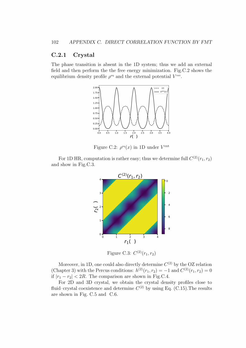
102 APPENDIX C. DIRECT CORRELATION FUNCTION BY FMT
C.2.1 Crystal
The phase transition is absent in the 1D system; thus we add an externalfield and then perform the the free energy minimization. Fig.C.2 shows theequilibrium density profile ρeq and the external potential V ext.
0.0 0.5 1.0 1.5 2.0 2.5 3.0 3.5 4.0r(σ)
0.00
0.25
0.50
0.75
1.00
1.25
1.50
1.75
2.00 ρ(r)Vext(r)
Figure C.2: ρeq(x) in 1D under V ext
For 1D HR, computation is rather easy; thus we determine full C(2)(r1, r2)and show in Fig.C.3.
0 1 2 3 4r1(σ)
0
1
2
3
4
r 2(σ)
C(2)(r1, r2)
−8
−6
−4
−2
0
Figure C.3: C(2)(r1, r2)
Moreover, in 1D, one could also directly determine C(2) by the OZ relation(Chapter 3) with the Percus conditions: h(2)(r1, r2) = −1 and C(2)(r1, r2) = 0if |r1 − r2| < 2R. The comparison are shown in Fig.C.4.
For 2D and 3D crystal, we obtain the crystal density profiles close tofluid–crystal coexistence and determine C(2) by using Eq. (C.15).The resultsare shown in Fig. C.5 and C.6.
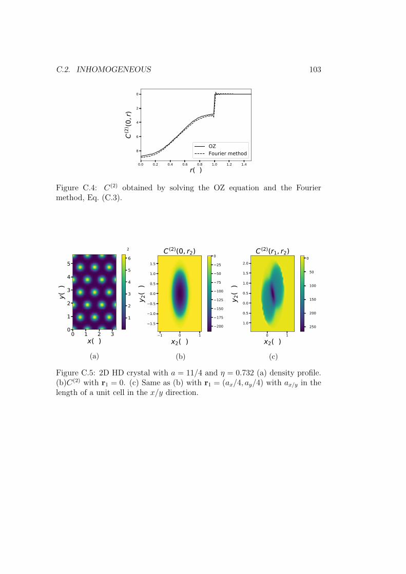
C.2. INHOMOGENEOUS 103
0.0 0.2 0.4 0.6 0.8 1.0 1.2 1.4r(σ)
−8
−6
−4
−2
0
C(2) (0
,r)
OZFourier method
Figure C.4: C(2) obtained by solving the OZ equation and the Fouriermethod, Eq. (C.3).
0 1 2 3x(σ)
0
1
2
3
4
5
y(σ)
ρσ2
1
2
3
4
5
6
(a)
−1 0 1x2(σ)
−1.5
−1.0
−0.5
0.0
0.5
1.0
1.5
y 2(σ)
C(2)(0, r2)
−200
−175
−150
−125
−100
−75
−50
−25
0
(b)
0 1x2(σ)
−1.0
−0.5
0.0
0.5
1.0
1.5
2.0
y 2(σ)
C(2)(r1, r2)
−250
−200
−150
−100
−50
0
(c)
Figure C.5: 2D HD crystal with a = 11/4 and η = 0.732 (a) density profile.(b)C(2) with r1 = 0. (c) Same as (b) with r1 = (ax/4, ay/4) with ax/y in thelength of a unit cell in the x/y direction.

104 APPENDIX C. DIRECT CORRELATION FUNCTION BY FMT
0 1 2 30.0
0.5
1.0
1.5
2.0
2.5
3.0
3.5
0
20
40
60
80
100
120
(a)
0.0 0.2 0.4 0.6 0.8 1.0r2
−60000
−50000
−40000
−30000
−20000
−10000
0
C(2) (0
,r2)
111110100
(b)
Figure C.6: C(2) in fcc structure with η = 0.545 and nvac = 2.18× 10⁻⁵. (a)density profile in xy–plane. (b) C(2) in three directions with r1 = 0
C.3 Conclusion
We have successfully obtained the C(2) for homogeneous and inhomogeneousfluid by FMT. However, for the 3D crystal, the requirement for computationalresources is still very high, for example the Fig C.6(b) takes one week with64 GPUs, and the further investigations for the relation between C(2) andmacroscopic crystal properties are required.
Bibliography
[1] G. Martius and C. H. Lampert, “Extrapolation and learning equations,”arXiv:1610.02995, 2016.
[2] S.-C. Lin and M. Oettel, “A classical density functional from machinelearning and a convolutional neural network,” SciPost Phys., vol. 6,p. 025, 2019.
[3] R. Roth, K. Mecke, and M. Oettel, “Communication: Fundamental mea-sure theory for hard disks: Fluid and solid,” J. Chem. Phys., vol. 136,p. 081101, 2012.
[4] Y. Rosenfeld, “Free–energy model for the inhomogeneous hard–spherefluid mixture and density–functional theory of freezing,” Phys. Rev.Lett., vol. 63, no. 9, p. 980, 1989.
[5] Y. Rosenfeld, M. Schmidt, H. Lowen, and P. Tarazona, “Fundamental–measure free–energy density functional for hard spheres: Dimensionalcrossover and freezing,” Phys. Rev. E, vol. 55, no. 4, p. 4245, 1997.
[6] P. Tarazona and Y. Rosenfeld, “From zero–dimension cavities to free–energy functionals for hard disks and hard spheres,” Phys. Rev. E,vol. 55, p. 4873, 1997.
[7] P. Tarazona, “Density functional for hard sphere crystals: A fundamen-tal measure approach,” Phys. Rev. Lett., vol. 84, p. 694, 2000.
[8] R. Roth, “Fundamental measure theory for hard–sphere mixtures: areview,” J. Phys.:Condens. Matter, vol. 22, no. 6, p. 063102, 2010.
[9] J. A. Barker and D. Henderson, “Perturbation theory and equation ofstate for fluids. II. A successful theory of liquids,” J. Chem. Phys, vol. 47,no. 11, pp. 4714–4721, 1967.
105
106 BIBLIOGRAPHY
[10] E. P. Bernard and W. Krauth, “Two–step melting in two dimensions:first–order liquid–hexatic transition,” Phys. Rev. Lett., vol. 107, no. 15,p. 155704, 2011.
[11] A. L. Thorneywork, J. L. Abbott, D. G. A. L. Aarts, and R. P. A.Dullens, “Two–dimensional melting of colloidal hard spheres,” Phys.Rev., vol. 118, no. 15, p. 158001, 2017.
[12] A. L. Thorneywork, R. Roth, D. G. A. L. Aarts, and R. P. A. Dul-lens, “Radial distribution functions in a two–dimensional binary col-loidal hard sphere system,” J. Chem. Phys., vol. 140, p. 161106, 2014.
[13] R. Castaneda-Priego, A. Rodrıguez-Lopez, and J. Mendez-Alcaraz, “De-pletion forces in two–dimensional colloidal mixtures,” J. Condens. Mat-ter Phys., vol. 15, no. 48, p. S3393, 2003.
[14] S. Asakura and F. Oosawa, “On interaction between two bodies im-mersed in a solution of macromolecules,” J. Chem. Phys, vol. 22, no. 7,pp. 1255–1256, 1954.
[15] S. Asakura and F. Oosawa, “Interaction between particles suspended insolutions of macromolecules,” J. Polym. Sci., vol. 33, no. 126, pp. 183–192, 1958.
[16] J. C. Snyder, M. Rupp, K. Hansen, K.-R. Muller, and K. Burke,“Finding density functionals with machine learning,” Phys. Rev. Lett.,vol. 108, p. 253002, 2012.
[17] L. Li, J. C. Snyder, I. M. Pelaschier, J. Huang, U.-N. Niranjan, P. Dun-can, M. Rupp, K.-R. Muller, and K. Burke, “Understanding machine–learned density functionals,” Int. J. Quantum Chem., vol. 116, p. 819,2016.
[18] F. Brockherde, L. Vogt, L. Li, M. E. Tuckerman, K. Burke, and K.-R.Muller, “Bypassing the Kohn–Sham equations with machine learning,”Nat. Commun., vol. 8, p. 872, 2017.
[19] J. Nelson, R. Tiwari, and S. Sanvito, “Machine learning density func-tional theory for the hubbard model,” Phys. Rev. B, vol. 99, p. 075132,2019.
[20] M. Bishop, “WCA perturbation theory for onedimensional Lennard–Jones fluids,” Am. J. Phys., vol. 52, p. 158, 1984.
BIBLIOGRAPHY 107
[21] M. Schmidt and H. Lipson, “Distilling free–form natural laws from ex-perimental data,” Science, vol. 324, p. 81, 2009.
[22] S. S. Sahoo, C. H. Lampert, and G. Martius, “Learning equations forextrapolation and control,” in Proceedings of the 35th International Con-ference on Machine Learning, vol. 80, pp. 4439–4447, PMLR, 10–15 Jul2018.
[23] J.-P. Hansen and I. R. McDonald, Theory of simple liquids: With appli-cations to soft matter. Academic Press, 2013.
[24] P. Hohenberg and W. Kohn, “Inhomogeneous electron gas,” Phys. Rev.,vol. 136, p. B864, 1964.
[25] N. D. Mermin, “Thermal properties of the inhomogeneous electron gas,”Physical Review, vol. 137, no. 5A, p. A1441, 1965.
[26] R. Evans, “The nature of the liquid–vapour interface and other topicsin the statistical mechanics of non–uniform, classical fluids,” Adv. Phys,vol. 28, no. 2, pp. 143–200, 1979.
[27] T. Ramakrishnan and M. Yussouff, “First–principles order–parametertheory of freezing,” Physical Review B, vol. 19, no. 5, p. 2775, 1979.
[28] Y. C. Chiew, “Percus–Yevick integral–equation theory for athermalhard–sphere chains: Part I: Equations of state,” Mol. Phys., vol. 70,no. 1, pp. 129–143, 1990.
[29] H. Hansen-Goos and R. Roth, “Density functional theory for hard–sphere mixtures: The white bear version mark II,” J. Phys. Condens.Matter, vol. 18, no. 37, p. 8413, 2006.
[30] H. Hansen-Goos and R. Roth, “A new generalization of the Carnahan–Starling equation of state to additive mixtures of hard spheres,” J.Chem. Phys, vol. 124, no. 15, p. 154506, 2006.
[31] M. Oettel, S. Gorig, A. Hartel, H. Lowen, M. Radu, and T. Schilling,“Free energies, vacancy concentrations, and density distributionanisotropies in hard–sphere crystals: A combined density functional andsimulation study,” Phys. Rev. E, vol. 82, no. 5, p. 051404, 2010.
[32] A. Hartel, M. Oettel, R. E. Rozas, S. U. Egelhaaf, J. Horbach, andH. Lowen, “Tension and stiffness of the hard sphere crystal–fluid inter-face,” Phys. Rev. Lett., vol. 108, p. 226101, 2012.

108 BIBLIOGRAPHY
[33] P. Tarazona, J. A. Cuesta, and Y. Martınez-Raton, “Density functionaltheories of hard particle systems,” in Theory and Simulation of Hard–Sphere Fluids and Related Systems, pp. 247–341, Springer, 2008.
[34] J. K. Percus, “Equilibrium state of a classical fluid of hard rods in anexternal field,” J. Stat. Phys., vol. 15, no. 6, pp. 505–511, 1976.
[35] M. Oettel, S. Dorosz, M. Berghoff, B. Nestler, and T. Schilling, “Descrip-tion of hard–sphere crystals and crystal–fluid interfaces: A comparisonbetween density functional approaches and a phase–field crystal model,”Phys. Rev. E, vol. 86, no. 2, p. 021404, 2012.
[36] J. Mellenthin, A. Karma, and M. Plapp, “Phase–field crystal studyof grain–boundary premelting,” Physical Review B, vol. 78, no. 18,p. 184110, 2008.
[37] A. Adland, A. Karma, R. Spatschek, D. Buta, and M. Asta, “Phase–field–crystal study of grain boundary premelting and shearing in bcciron,” Phys. Rev. B, vol. 87, no. 2, p. 024110, 2013.
[38] R. C. Tolman, “Consideration of the Gibbs theory of surface tension,”J. Chem. Phys, vol. 16, no. 8, pp. 758–774, 1948.
[39] R. C. Tolman, “The effect of droplet size on surface tension,” J. Chem.Phys, vol. 17, no. 3, pp. 333–337, 1949.
[40] G. I. Toth and L. Granasy, “Crystal nucleation in the hard–sphere sys-tem revisited: A critical test of theoretical approaches,” J. Phys. Chem.B, vol. 113, no. 15, pp. 5141–5148, 2009.
[41] P. Montero de Hijes, J. R. Espinosa, V. Bianco, E. Sanz, and C. Vega,“Interfacial free energy and tolman length of curved liquid–solid inter-faces from equilibrium studies,” J. Phys. Chem. C, vol. 124, no. 16,pp. 8795–8805, 2020.
[42] A. Cacciuto, S. Auer, and D. Frenkel, “Solid–liquid interfacial free en-ergy of small colloidal hard–sphere crystals,” J. Chem. Phys, vol. 119,no. 14, pp. 7467–7470, 2003.
[43] P. R. ten Wolde and D. Frenkel, “Computer simulation study of gas–liquid nucleation in a Lennard–Jones system,” J. Chem. Phys, vol. 109,no. 22, pp. 9901–9918, 1998.

BIBLIOGRAPHY 109
[44] M. Moody and P. Attard, “Curvature dependent surface tension from asimulation of a cavity in a Lennard–Jones liquid close to coexistence,”J. Chem. Phys, vol. 115, no. 19, pp. 8967–8977, 2001.
[45] J. C. Barrett, “Some estimates of the surface tension of curved sur-faces using density functional theory,” J. Chem. Phys, vol. 124, no. 14,p. 144705, 2006.
[46] N. Bruot and F. Caupin, “Curvature dependence of the liquid–vaporsurface tension beyond the tolman approximation,” Phys. Rev. Lett.,vol. 116, no. 5, p. 056102, 2016.
[47] A. Troter, F. Schmitz, P. Virnau, and K. Binder, “Equilibrium betweena droplet and surrounding vapor: A discussion of finite size effects,” J.Phys. Chem. B, vol. 122, no. 13, pp. 3407–3417, 2017.
[48] A. Troster and K. Binder, “Positive Tolman length in a lattice gas withthree–body interactions,” Phys. Rev., vol. 107, no. 26, p. 265701, 2011.
[49] J. M. Kosterlitz and D. Thouless, “Long range order and metastabilityin two dimensional solids and superfluids. (Application of dislocationtheory),” J Phys C: Solid State Phys, vol. 5, no. 11, p. L124, 1972.
[50] J. M. Kosterlitz and D. J. Thouless, “Ordering, metastability and phasetransitions in two–dimensional systems,” J Phys C: Solid State Phys,vol. 6, no. 7, p. 1181, 1973.
[51] B. Halperin and D. R. Nelson, “Theory of two–dimensional melting,”Phys. Rev. Lett., vol. 41, no. 2, p. 121, 1978.
[52] D. R. Nelson and B. Halperin, “Dislocation–mediated melting in twodimensions,” Physical Review B, vol. 19, no. 5, p. 2457, 1979.
[53] A. Young, “Melting and the vector Coulomb gas in two dimensions,”Physical Review B, vol. 19, no. 4, p. 1855, 1979.
[54] K. J. Strandburg, “Two–dimensional melting,” Rev. Mod. Phys., vol. 60,no. 1, p. 161, 1988.
[55] S.-C. Lin and M. Oettel, “Phase diagrams and crystal–fluid surfacetensions in additive and nonadditive two–dimensional binary hard–diskmixtures,” Phys. Rev. E, vol. 98, no. 1, p. 012608, 2018.

110 BIBLIOGRAPHY
[56] J. M. Brader, R. Evans, and M. Schmidt, “Statistical mechanics of in-homogeneous model colloid–polymer mixtures,” Mol. Phys., vol. 101,p. 3349, 2003.
[57] M. Mortazavifar and M. Oettel, “A fundamental measure density func-tional for fluid and crystal phases of the Asakura–Oosawa model,” J.Phys.:Condens. Matter, vol. 28, no. 24, p. 244018, 2016.
[58] C. N. Likos and C. L. Henley, “Complex alloy phases for binary hard–disc mixtures,” Philos. Mag. B, vol. 68, p. 85, 1993.
[59] J. Russo and N. B. Wilding, “Disappearance of the hexatic phase in a bi-nary mixture of hard disks,” Phys. Rev. Lett., vol. 119, no. 11, p. 115702,2017.
[60] W. G. T. Kranendonk and D. Frenkel, “Computer simulation of solid–liquid coexistence in binary hard sphere mixtures,” Mol. Phys., vol. 72,p. 679, 1991.
[61] M. Oettel, “Mode expansion for the density profiles of crystal–fluid in-terfaces: hard spheres as a test case,” J. Phys.:Condens. Matter, vol. 24,no. 46, p. 464124, 2012.
[62] R. L. Vink, T. Neuhaus, and H. Lowen, “Fluid phase separation in-side a static periodic field: An effectively two–dimensional critical phe-nomenon,” J. Chem. Phys., vol. 134, no. 20, p. 204907, 2011.
[63] A. E. Gonzalez, “Colloidal crystallization in 2D for short–ranged attrac-tions: A descriptive overview,” Crystals, vol. 6, p. 46, 2016.
[64] M. Amini and B. B. Laird, “Crystal–melt interfacial free energy of bi-nary hard spheres from capillary fluctuations,” Phys. Rev. B, vol. 78,p. 144112, 2008.
[65] C. A. Becker, D. L. Olmsted, M. Asta, J. J. Hoyt, and S. M. Foiles,“Atomistic simulations of crystal–melt interfaces in a model binary alloy:Interfacial free energies, adsorption coefficients, and excess entropy,”Phys. Rev. B, vol. 79, p. 054109, 2009.
[66] J. Percus, “Entropy of a non–uniform one–dimensional fluid,” J. Con-dens. Matter Phys., vol. 1, no. 17, p. 2911, 1989.
[67] M. A. Kramer, “Nonlinear principal component analysis using autoas-sociative neural networks,” AIChE journal, vol. 37, no. 2, pp. 233–243,1991.
BIBLIOGRAPHY 111
[68] P. Mehta, M. Bukov, C.-H. Wang, A. G. Day, C. Richardson, C. K.Fisher, and D. J. Schwab, “A high–bias, low–variance introduction tomachine learning for physicists,” Phys. Rep., 2019.
[69] M. Abadi, A. Agarwal, P. Barham, E. Brevdo, Z. Chen, C. Citro, G. S.Corrado, A. Davis, J. Dean, M. Devin, S. Ghemawat, I. Goodfellow,A. Harp, G. Irving, M. Isard, Y. Jia, R. Jozefowicz, L. Kaiser, M. Kud-lur, J. Levenberg, D. Mane, R. Monga, S. Moore, D. Murray, C. Olah,M. Schuster, J. Shlens, B. Steiner, I. Sutskever, K. Talwar, P. Tucker,V. Vanhoucke, V. Vasudevan, F. Viegas, O. Vinyals, P. Warden, M. Wat-tenberg, M. Wicke, Y. Yu, and X. Zheng, “TensorFlow: Large–scalemachine learning on heterogeneous systems,” 2015. Software availablefrom tensorflow.org.
[70] A. Paszke, S. Gross, F. Massa, A. Lerer, J. Bradbury, G. Chanan,T. Killeen, Z. Lin, N. Gimelshein, L. Antiga, et al., “Pytorch: An im-perative style, high–performance deep learning library,” in Advances inneural information processing systems, pp. 8026–8037, 2019.
[71] A. J. Archer, B. Chacko, and R. Evan, “The standard mean–field treat-ment of inter–particle attraction in classical dft is better than one mightexpect,” J. Chem. Phys., vol. 147, p. 034501, 2017.
[72] K. R. Elder, N. Provatas, J. Berry, P. Stefanovic, and M. Grant, “Phase–field crystal modeling and classical density functional theory of freezing,”Phys. Rev. B, vol. 75, no. 6, p. 064107, 2007.
[73] M. Wertheim, “Fluids with highly directional attractive forces. i. Sta-tistical thermodynamics,” J. Stat. Phys., vol. 35, no. 1–2, pp. 19–34,1984.
[74] D. Stopper, F. Hirschmann, M. Oettel, and R. Roth, “Bulk structuralinformation from density functionals for patchy particles,” J. Chem.Phys, vol. 149, no. 22, p. 224503, 2018.
[75] S.-C. Lin, G. Martius, and M. Oettel, “Analytical classical density func-tionals from an equation learning network,” J. Chem. Phys, vol. 152,no. 2, p. 021102, 2020.
[76] H. Hansen-Goos and K. Mecke, “Fundamental measure theory for in-homogeneous fluids of nonspherical hard particles,” Phys. Rev. Lett.,vol. 102, p. 018302, 2009.
112 BIBLIOGRAPHY
[77] R. Wittmann, M. Marechal, and K. Mecke, “Fundamental mixed mea-sure theory for non–spherical colloids,” EPL, vol. 109, p. 26003, 2015.
[78] M. Oettel, M. Klopotek, M. Dixit, E. Empting, T. Schilling, andH. Hansen-Goos, “Monolayers of hard rods on planar substrates: I.Equilibrium,” J. Chem. Phys., vol. 145, p. 074902, 2016.
[79] D. P. Kingma and J. Ba, “Adam: A method for stochastic optimization,”arXiv:1412.6980, 2014.
[80] R. Tibshirani, “Regression shrinkage and selection via the lasso,” J. R.Stat. Soc. Series B Stat. Methodol., pp. 267–288, 1996.
[81] J. A. Cuesta and A. Sanchez, “General non–existence theorem for phasetransitions in one–dimensional systems with short range interactions,and physical examples of such transitions,” J. Stat. Phys., vol. 115,no. 3–4, pp. 869–893, 2004.
[82] V. P. Sergiievskyi, G. Jeanmairet, M. Levesque, and D. Borgis, “Fastcomputation of solvation free energies with molecular density functionaltheory: Thermodynamic–ensemble partial molar volume corrections,”J. Phys. Chem. Lett., vol. 5, no. 11, pp. 1935–1942, 2014.
[83] G. Jeanmairet, M. Levesque, R. Vuilleumier, and D. Borgis, “Moleculardensity functional theory of water,” J. Phys. Chem. Lett., vol. 4, no. 4,pp. 619–624, 2013.
[84] G. Jeanmairet, M. Levesque, and D. Borgis, “Molecular density func-tional theory of water describing hydrophobicity at short and long lengthscales,” J. Chem. Phys., vol. 139, no. 15, p. 154101, 2013.
[85] M. Mortazavifar, Equilibrium properties of crystals in the hard–sphereand the Asakura–Oosawa Model. PhD thesis, Eberhard Karls Univer-sitat Tubingen, 2016.
[86] T. Bernet, E. A. Muller, and G. Jackson, “A tensorial fundamentalmeasure density functional theory for the description of adsorption insubstrates of arbitrary three–dimensional geometry,” J. Chem. Phys,vol. 152, no. 22, p. 224701, 2020.
[87] M. Frigo and S. G. Johnson, “FFTW user’s manual,” MassachusettsInstitute of Technology, 1999.

BIBLIOGRAPHY 113
[88] D. Stopper and R. Roth, “Massively parallel GPU–accelerated mini-mization of classical density functional theory,” J. Chem. Phys., vol. 147,no. 6, p. 064508, 2017.
[89] S. Johnson, “Notes on FFT–based differentiation,” 2011. Available fromhttps://math.mit.edu/~stevenj/notes.html.
[90] A. Hartel, Density functional theory of hard colloidal particles: Frombulk to interfaces. PhD thesis, Universitat Dusseldorf, 2013.
[91] P. Pulay, “Convergence acceleration of iterative sequences. the case ofSCF iteration,” Chem. Phys. Lett., vol. 73, no. 2, pp. 393–398, 1980.
[92] S. A. Orszag, “Numerical methods for the simulation of turbulence,”Phys. Fluids, vol. 12, no. 12, pp. II–250, 1969.

Acknowledgment
In July 2016, I moved to Tubingen, Germany. At that time I joined alanguage school and searched for Ph.D. positions. Fortunately, Prof. Dr.Martin Oettel offered me a research assistant work and helped me applyingfor scholarships. In April 2017, I obtained the state fund scholarship (Lan-desgraduiertenforderungsgesetzes) from Baden–Wurttemberg and started myPh.D. works.
In the beginning, Martin suggested tackling dynamic density functionaltheory (DDFT) for hard–spheres crystals. With certain investigations andimprovements, we were able to stabilize the crystals but crystal-fluid in-terfaces are still unstable. After about six months, we shifted to two–dimensional hard–disk binary systems, where the numerical difficulty is muchlower and thus we systemically investigated the phase-diagrams and crystal–fluid interfaces.
By the time summarizing and publishing the results of hard–disks mix-tures, I started thinking whether there is a better way to obtain the free en-ergy functionals for arbitrary particle–particle interactions. This is a decades–long problem in DFT: how to go beyond mean–field approximation? Whilethere are almost exact functionals for hard–spheres systems, the tail partsthat treated by the mean–field approximation always spoils the accuracy ofthe functional. In December 2017, Dr. Daniel de las Heras was invited togive a talk about using machine learning to obtain the external potential bydensity distributions. At the end of the talk, Prof. Dr. Roth asked: “Canmachine learning give us density functionals ?”. This question became aseed in my mind. After about one–month literature research and some pre-liminary results, Martin was convinced that it is worth investigating more.After that, we published the first paper that uses convolutional networks toobtain the explicit functionals with simple ansatze. Furthermore, we collab-orated with Dr. Georg Martius to extend the flexibility and reliability of thenetwork and learned functionals.
I want to thanks Dr. Mortazavifar, Dr. Joachim Schope, Dr. Bleibel andDr. Stopper for their insightful discussions and constructive suggestions. I
115

116 BIBLIOGRAPHY
also thank my dear colleagues Miriam, Paul, Frank, Eelo, Malte, and Manuelfor their supports in this thesis and helps me understanding German culture;especially Miriam, without her I probably gave up the ML ideas already.
I thank my supervisor, Prof. Dr. Martin Oettel for his enthusiasticcooperation, deep understanding of colloid systems, constructive discussions,great support and thoughtful help throughout my Ph.D. studies. Withouthim, I have no chance to do my Ph.D. I acknowledge my second supervisorProf. Dr. Roth, who helps me for achieving a deeper understanding of DFT.Also, I acknowledge Dr. Georg Martius, who helps me improving my MLknowledge.
Finally, I thanks my ex-wife. Just kidding, no.