Paper ID #6099

QUICK-RETURN MECHANISM REVISITED

Prof. Raghu Echempati, Kettering University

Raghu Echempati is a professor and graduate programs director of Mechanical Engineering at Ketter-ing with academic experience of over 25 years. His areas of expertise are Mechanics, CAE, MechanismDesign, Mechanical Engineering Design, Vibrations, Finite Element Analysis and Sheet Metal FormingSimulation. He is a fellow member, advisor and chair of the ASME local chapters. Also, he is a memberof ASEE and SAE. He is a co-organizer of Body Design and Engineering Session of SAE World Congressand an associate editor of Journal of Passenger Cars. He has delivered lectures, short term courses andworkshops at several national and international conferences. The countries include Argentina, Australia,Brazil, Germany, Korea, India, USA and Taiwan. He taught several three-month terms in Germany atHTWG-Konstanz, Konstanz. He promotes applied research and consulting and also study abroad pro-grams. Dr. Echempati is a winner of several awards for his services to the academic and professionalcommunities.

Mr. Theodore Paul DaniMs. Ankita SahuMr. Nathan Marshall LeBlanc

c©American Society for Engineering Education, 2013

Work In Progress: Quick-Return Mechanism Revisited

Abstract

In this paper, the teaching and learning experiences of the author with two summer interns at one

of the educational institutions in India is presented. These are the senior mechanical engineering

students from two different engineering colleges in India who spent nearly two months at the

institute where the author spent a 3-month sabbatical as a visiting faculty. Although these two

students took the “Theory of Machines” course at their college, a complete understanding of

kinematic and dynamic analyses of mechanisms such as a quick-return linkage seemed to be not

realized well by them. In addition to the students from India, there are other mechanical

engineering students who were taking a Design and Analysis of Mechanical Systems and

Assemblies course as a directed study. The students were taught the basics of loop-closure

equations pertaining to the kinematic and dynamic analysis of an example quick-return and other

planar mechanisms. All these students developed an Excel based program to perform

calculations and plot the various characteristics such as variation of quick return ratio as a

function of the critical link lengths, kinematic and dynamic characteristics of the linkage. Studies

related to partially balance the system are also under way, mostly using a CAE tool. The students

modeled the linkage using the motion simulation application that is commonly available in any

CAE tool such as Catia, UG-NX, NX I-DEAS, or SolidWorks. Other math tools such as MatLab

Simulink, MapleSim, etc., are also available to study planar mechanism kinematics. Finally, the

students in India used the available laboratory experimental apparatus to verify some of the

theoretical calculations. The performance metric is a final report that included the learning

outcomes and recommendations for further work.

Introduction and literature review

The Course Learning Objectives (CLOs) of the course are:

1. Apply the integration of the fundamental concepts of rigid body kinematics in relative

motion, solid mechanics and computer aided engineering through computational and

design tools.

2. Apply fundamental mechanics principles to the kinematic, dynamic and fatigue stress analyses of components of planar mechanisms, subsystems and systems.

3. Use state-of-the-art CAE software tools to formulate, conceptualize, design, analyze, and synthesize open-ended problems pertaining to mechanical systems.

4. Develop strategies to improve the product and process design based on the results

obtained.

In tune with the above CLOs, students the course is taught using a combination of theory using

graphical and analytical methods and CAE tools such as I-DEAS or NX 7.5. However, covering

in depth theory using analytical kinematics is found to be challenging due to time constraints. On

the other hand, the conventional graphical methods although limited to analysis of a mechanism

in the instantaneous reference frame, students seem to realize their ease of use. In order to

expand the students understanding of mechanisms, it is important to explore the same system at

multiple points in time, delivering an understanding of the cycle the mechanism would go

through during operation. It is common for students and researchers to explore the use of

software to design and analyze mechanism cycles using CAE tools such as Catia, Unigraphics-

NX, HyperWorks, NX I-DEAS or SolidWorks1-5

. Also mathematical tools such as MapleSim6

and Matlab7 and written programs such as C

++, Fortran and T-K Solver

8-10, etc are also used.

However, the use of these programs does not require the student to have a deeper understanding

of the methods being used in the analysis. In the case of software such as C++, Matlab, and

Maplesim the student does not have a visual representation of how the model behaves while in

motion. Conversely, to use solid modeling and simulations software such as Solidworks and UG-

NX the student is not required to have a full understanding of the methods being used in the

analysis. In order to allow students to analyze an example model while still understanding the

methods involved, an analysis program for a Whitworth quick-return mechanism was created in

Microsoft excel. The same model was modeled in a CAE software and motion was simulated to

create a reference for verification of the excel model. The model was further cross referenced to

a previously published work on the use of a C++

program that provided a solution to the example

in question11

. The example used is the Whitworth quick-return system, an uncommonly explored

linkage because it has not been used in high frequency application due to fundamental

difficulties with unbalance and vibrations. The Microsoft Excel program generated in this report

is eventually to be expanded upon with the interest of exploring methods to balance the system,

reducing vibrations in and expanding on the applications of this mechanism. A physical model

was subsequently used by the students in India to acquire data and verify the authenticity of the

equations and models.

Analysis

The model analyzed in this paper was replicated from a previous paper that explored the use of

C++

programing to fully model a Whitworth Quick return mechanism published by Matt

Campbell and Stephan Nestinger11

. In the interests of cross referential verification, the model

simulated in this paper is the same as the model in the previously published paper.

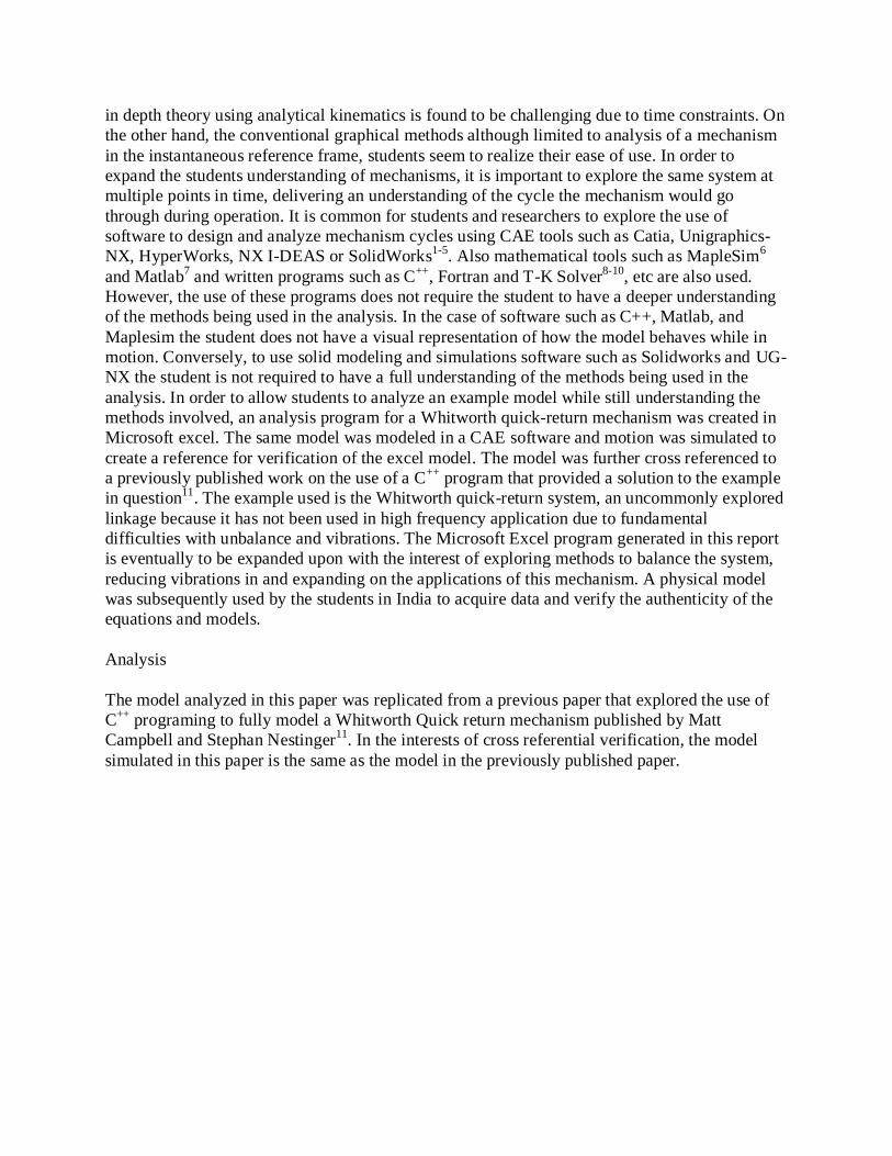
Figure 1. Vector representation of the Whitworth Quick Return Mechanism 11

The equations for Kinematic analysis that are presented below were originally presented by

Campbell and Nestinger11

.

Position Analysis:

The displacement analysis can be formulated by following equations:

(1a)

(1b)

Using complex numbers, Equations 1 and 2 become

(2a)

(2b)

Here, link lengths and angular positions are constants.

Now, equ.1 becomes

(3a)

And since, .

Therefore, equ.4 can be written as,

(3b)

Using Euler’s equation,

,

(4a)

(4b)

Squaring Equations 4, adding them together, we get

(5)

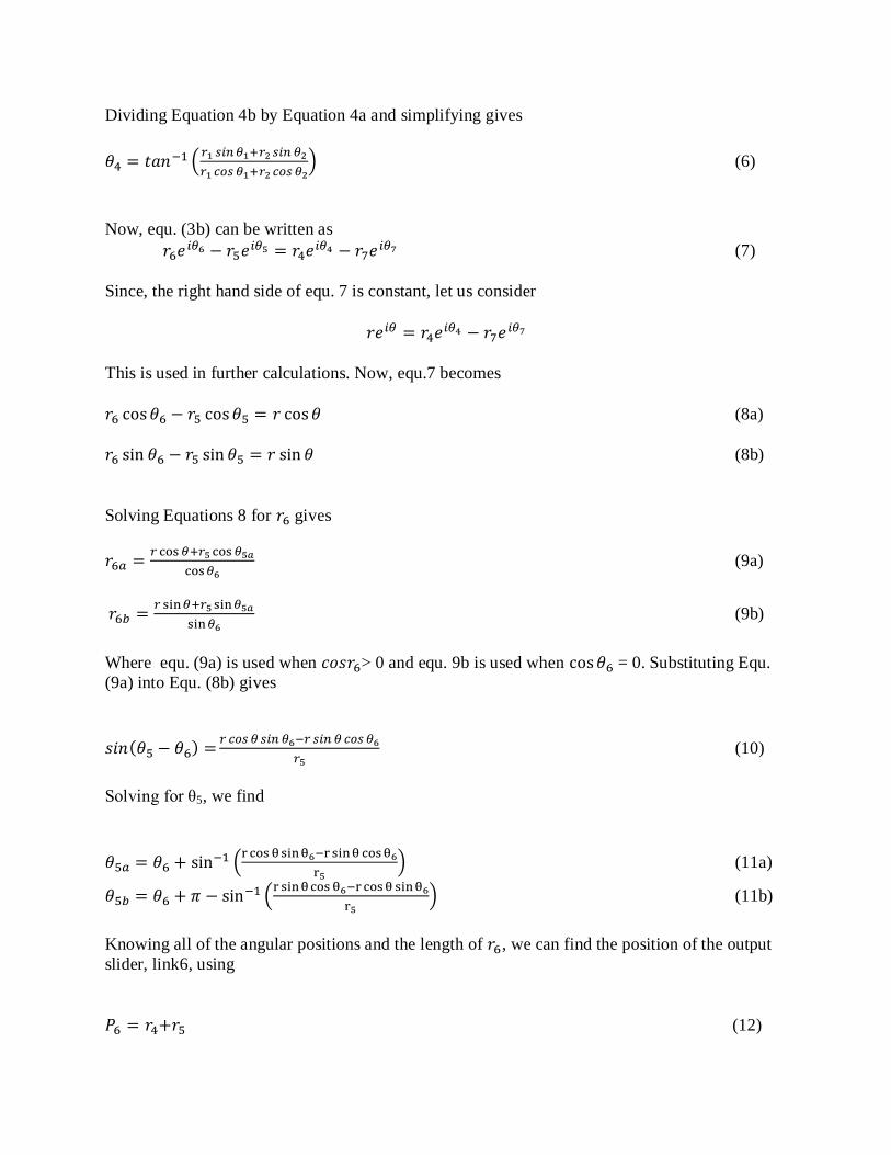
Dividing Equation 4b by Equation 4a and simplifying gives

(6)

Now, equ. (3b) can be written as

(7)

Since, the right hand side of equ. 7 is constant, let us consider

This is used in further calculations. Now, equ.7 becomes

(8a)

(8b)

Solving Equations 8 for gives

(9a)

(9b)

Where equ. (9a) is used when > 0 and equ. 9b is used when = 0. Substituting Equ.

(9a) into Equ. (8b) gives

(10)

Solving for θ5, we find

(11a)

(11b)

Knowing all of the angular positions and the length of , we can find the position of the output

slider, link6, using

(12)

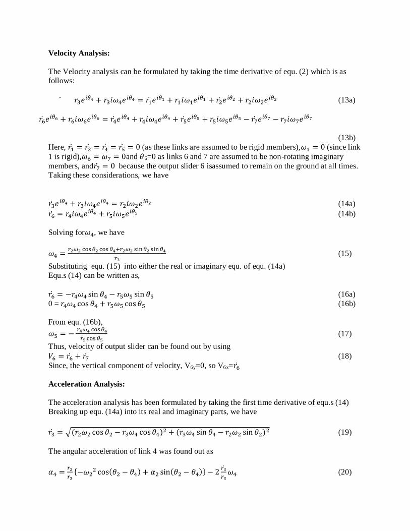
Velocity Analysis:

The Velocity analysis can be formulated by taking the time derivative of equ. (2) which is as

follows:

(13a)

(13b)

Here, (as these links are assumed to be rigid members), (since link

1 is rigid), and 6=0 as links 6 and 7 are assumed to be non-rotating imaginary

members, and because the output slider 6 isassumed to remain on the ground at all times.

Taking these considerations, we have

(14a)

(14b)

Solving for , we have

(15)

Substituting equ. (15) into either the real or imaginary equ. of equ. (14a)

Equ.s (14) can be written as,

(16a)

0 = (16b)

From equ. (16b),

(17)

Thus, velocity of output slider can be found out by using

(18)

Since, the vertical component of velocity, V6y=0, so V6x=

Acceleration Analysis:

The acceleration analysis has been formulated by taking the first time derivative of equ.s (14)

Breaking up equ. (14a) into its real and imaginary parts, we have

(19)

The angular acceleration of link 4 was found out as

(20)

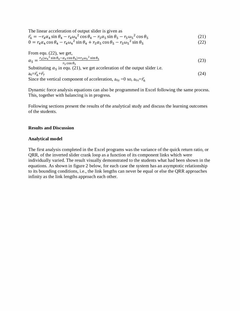
The linear acceleration of output slider is given as

(21)

(22)

From equ. (22), we get,

(23)

Substituting in equ. (21), we get acceleration of the output slider i.e.

a6= + (24)

Since the vertical component of acceleration, a6y =0 so, a6x=

Dynamic force analysis equations can also be programmed in Excel following the same process.

This, together with balancing is in progress.

Following sections present the results of the analytical study and discuss the learning outcomes

of the students.

Results and Discussion

Analytical model

The first analysis completed in the Excel programs was the variance of the quick return ratio, or

QRR, of the inverted slider crank loop as a function of its component links which were

individually varied. The result visually demonstrated to the students what had been shown in the

equations. As shown in figure 2 below, for each case the system has an asymptotic relationship

to its bounding conditions, i.e., the link lengths can never be equal or else the QRR approaches

infinity as the link lengths approach each other.

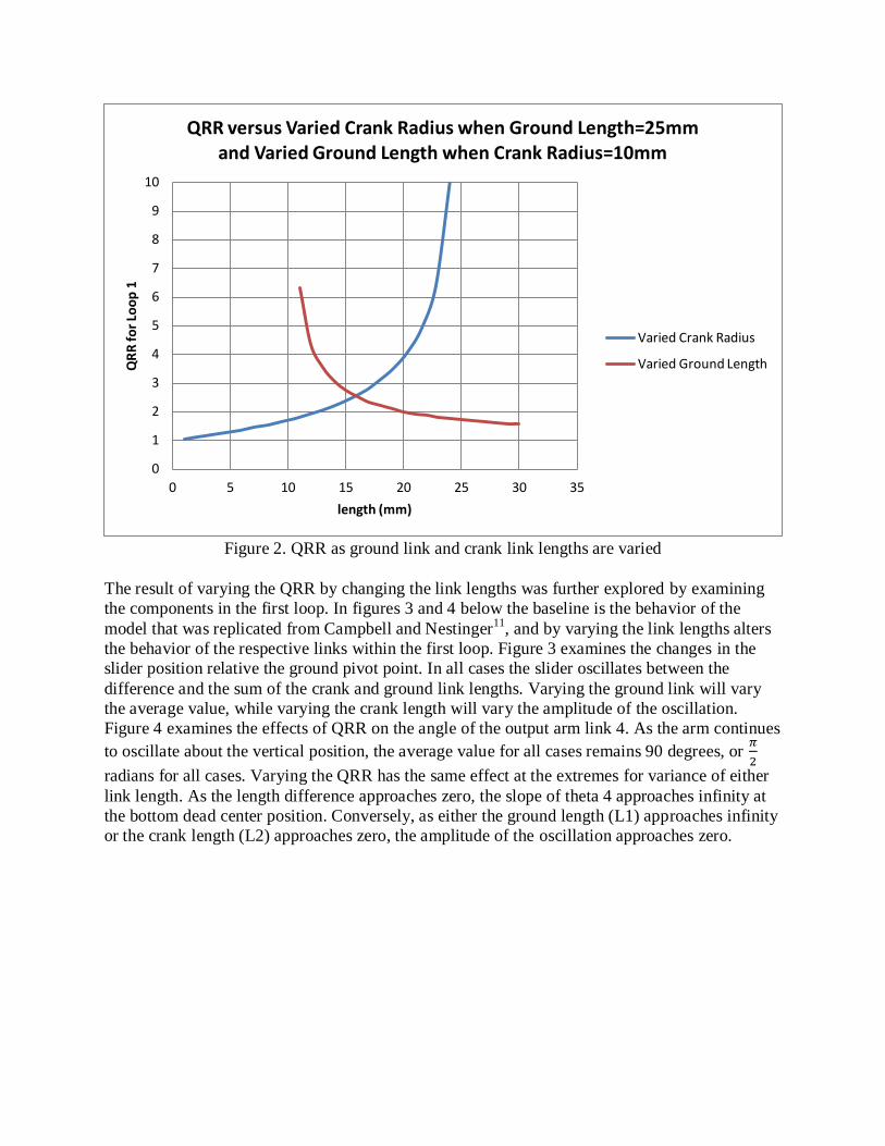
Figure 2. QRR as ground link and crank link lengths are varied

The result of varying the QRR by changing the link lengths was further explored by examining

the components in the first loop. In figures 3 and 4 below the baseline is the behavior of the

model that was replicated from Campbell and Nestinger11

, and by varying the link lengths alters

the behavior of the respective links within the first loop. Figure 3 examines the changes in the

slider position relative the ground pivot point. In all cases the slider oscillates between the

difference and the sum of the crank and ground link lengths. Varying the ground link will vary

the average value, while varying the crank length will vary the amplitude of the oscillation.

Figure 4 examines the effects of QRR on the angle of the output arm link 4. As the arm continues

to oscillate about the vertical position, the average value for all cases remains 90 degrees, or

radians for all cases. Varying the QRR has the same effect at the extremes for variance of either

link length. As the length difference approaches zero, the slope of theta 4 approaches infinity at

the bottom dead center position. Conversely, as either the ground length (L1) approaches infinity

or the crank length (L2) approaches zero, the amplitude of the oscillation approaches zero.

0

1

2

3

4

5

6

7

8

9

10

0 5 10 15 20 25 30 35

QR

R fo

r Lo

op

1

length (mm)

QRR versus Varied Crank Radius when Ground Length=25mm and Varied Ground Length when Crank Radius=10mm

Varied Crank Radius

Varied Ground Length

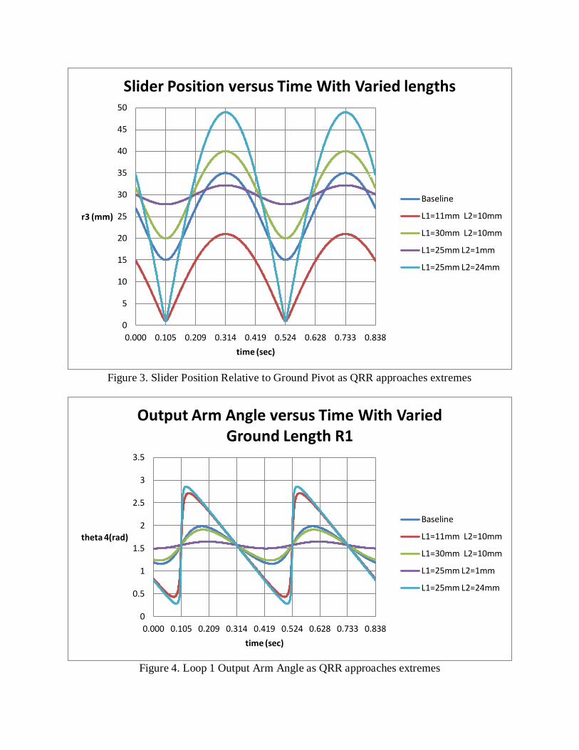
Figure 3. Slider Position Relative to Ground Pivot as QRR approaches extremes

Figure 4. Loop 1 Output Arm Angle as QRR approaches extremes

0

5

10

15

20

25

30

35

40

45

50

0.000 0.105 0.209 0.314 0.419 0.524 0.628 0.733 0.838

r3 (mm)

time (sec)

Slider Position versus Time With Varied lengths

Baseline

L1=11mm L2=10mm

L1=30mm L2=10mm

L1=25mm L2=1mm

L1=25mm L2=24mm

0

0.5

1

1.5

2

2.5

3

3.5

0.000 0.105 0.209 0.314 0.419 0.524 0.628 0.733 0.838

theta 4(rad)

time (sec)

Output Arm Angle versus Time With Varied Ground Length R1

Baseline

L1=11mm L2=10mm

L1=30mm L2=10mm

L1=25mm L2=1mm

L1=25mm L2=24mm

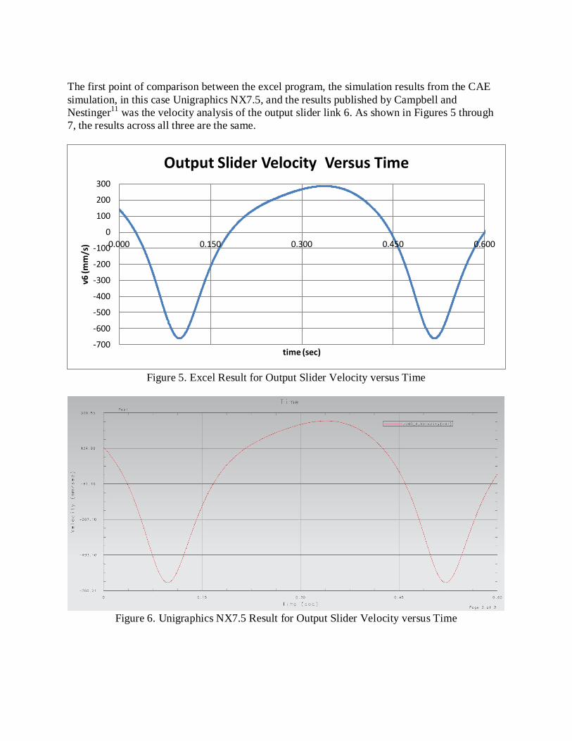
The first point of comparison between the excel program, the simulation results from the CAE

simulation, in this case Unigraphics NX7.5, and the results published by Campbell and

Nestinger11

was the velocity analysis of the output slider link 6. As shown in Figures 5 through

7, the results across all three are the same.

Figure 5. Excel Result for Output Slider Velocity versus Time

Figure 6. Unigraphics NX7.5 Result for Output Slider Velocity versus Time

-700

-600

-500

-400

-300

-200

-100

0

100

200

300

0.000 0.150 0.300 0.450 0.600

v6 (m

m/s

)

time (sec)

Output Slider Velocity Versus Time

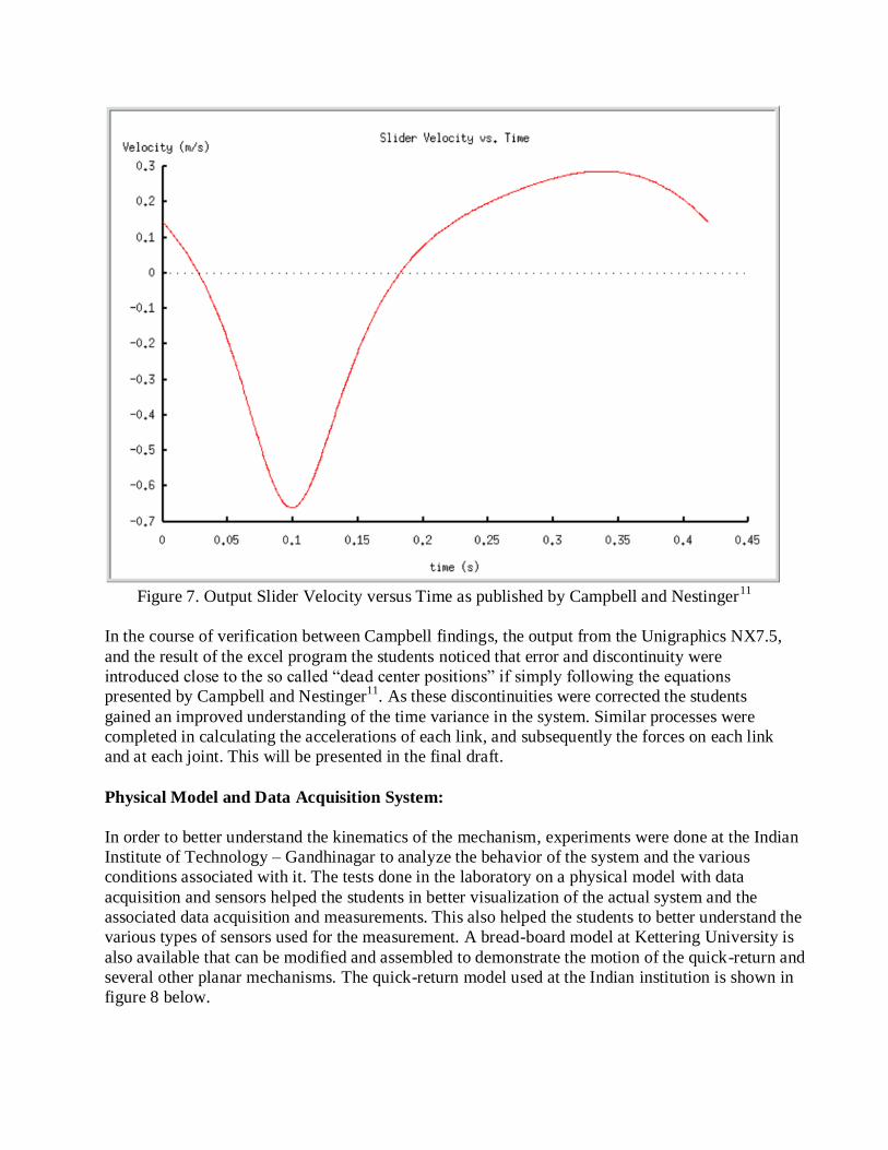
Figure 7. Output Slider Velocity versus Time as published by Campbell and Nestinger

11

In the course of verification between Campbell findings, the output from the Unigraphics NX7.5,

and the result of the excel program the students noticed that error and discontinuity were

introduced close to the so called “dead center positions” if simply following the equations

presented by Campbell and Nestinger11

. As these discontinuities were corrected the students

gained an improved understanding of the time variance in the system. Similar processes were

completed in calculating the accelerations of each link, and subsequently the forces on each link

and at each joint. This will be presented in the final draft.

Physical Model and Data Acquisition System:

In order to better understand the kinematics of the mechanism, experiments were done at the Indian

Institute of Technology – Gandhinagar to analyze the behavior of the system and the various

conditions associated with it. The tests done in the laboratory on a physical model with data

acquisition and sensors helped the students in better visualization of the actual system and the

associated data acquisition and measurements. This also helped the students to better understand the

various types of sensors used for the measurement. A bread-board model at Kettering University is

also available that can be modified and assembled to demonstrate the motion of the quick-return and

several other planar mechanisms. The quick-return model used at the Indian institution is shown in

figure 8 below.

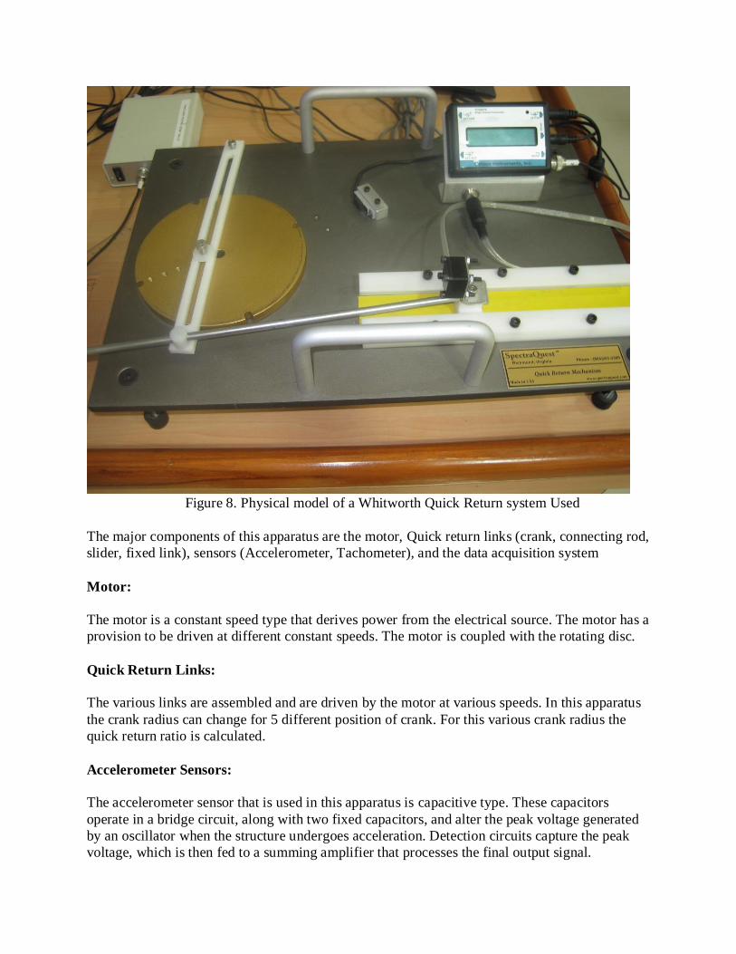
Figure 8. Physical model of a Whitworth Quick Return system Used

The major components of this apparatus are the motor, Quick return links (crank, connecting rod,

slider, fixed link), sensors (Accelerometer, Tachometer), and the data acquisition system

Motor:

The motor is a constant speed type that derives power from the electrical source. The motor has a

provision to be driven at different constant speeds. The motor is coupled with the rotating disc.

Quick Return Links:

The various links are assembled and are driven by the motor at various speeds. In this apparatus

the crank radius can change for 5 different position of crank. For this various crank radius the

quick return ratio is calculated.

Accelerometer Sensors:

The accelerometer sensor that is used in this apparatus is capacitive type. These capacitors

operate in a bridge circuit, along with two fixed capacitors, and alter the peak voltage generated

by an oscillator when the structure undergoes acceleration. Detection circuits capture the peak

voltage, which is then fed to a summing amplifier that processes the final output signal.

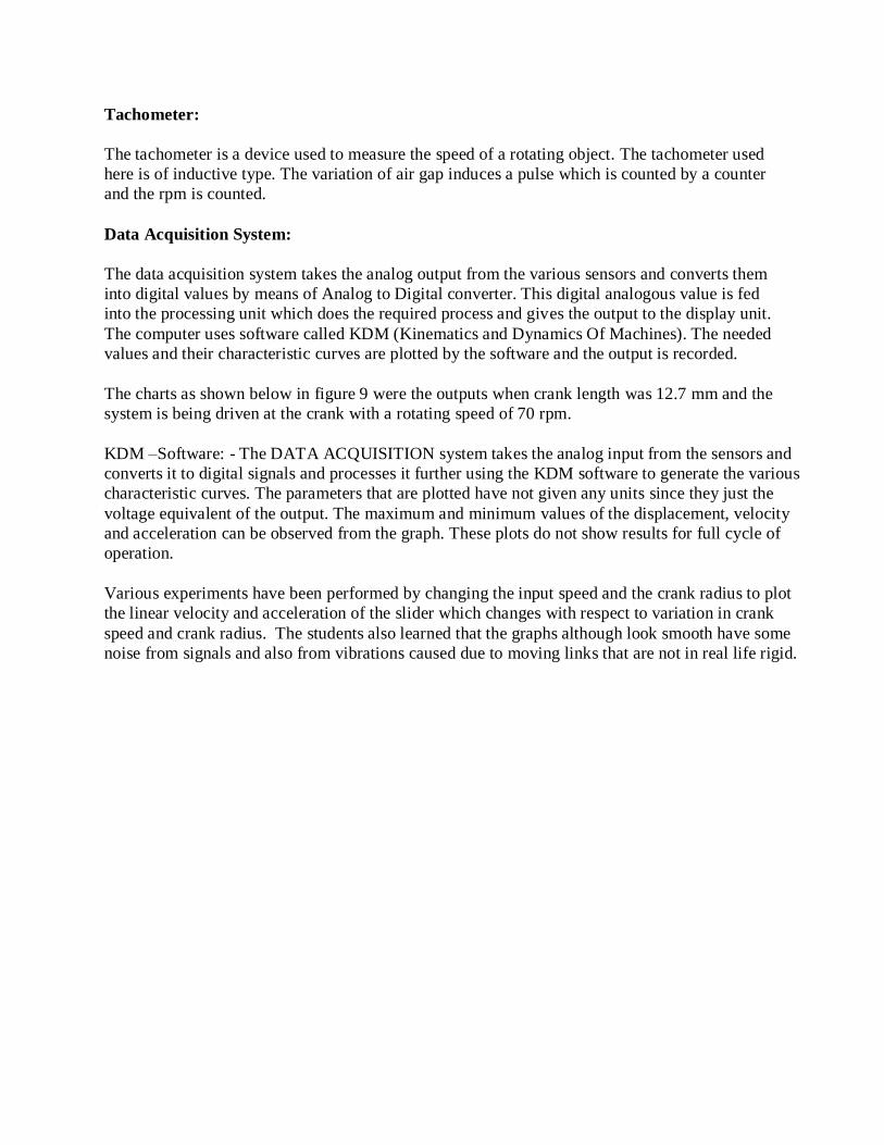
Tachometer:

The tachometer is a device used to measure the speed of a rotating object. The tachometer used

here is of inductive type. The variation of air gap induces a pulse which is counted by a counter

and the rpm is counted.

Data Acquisition System:

The data acquisition system takes the analog output from the various sensors and converts them

into digital values by means of Analog to Digital converter. This digital analogous value is fed

into the processing unit which does the required process and gives the output to the display unit.

The computer uses software called KDM (Kinematics and Dynamics Of Machines). The needed

values and their characteristic curves are plotted by the software and the output is recorded.

The charts as shown below in figure 9 were the outputs when crank length was 12.7 mm and the

system is being driven at the crank with a rotating speed of 70 rpm.

KDM –Software: - The DATA ACQUISITION system takes the analog input from the sensors and

converts it to digital signals and processes it further using the KDM software to generate the various

characteristic curves. The parameters that are plotted have not given any units since they just the

voltage equivalent of the output. The maximum and minimum values of the displacement, velocity

and acceleration can be observed from the graph. These plots do not show results for full cycle of

operation.

Various experiments have been performed by changing the input speed and the crank radius to plot

the linear velocity and acceleration of the slider which changes with respect to variation in crank

speed and crank radius. The students also learned that the graphs although look smooth have some

noise from signals and also from vibrations caused due to moving links that are not in real life rigid.

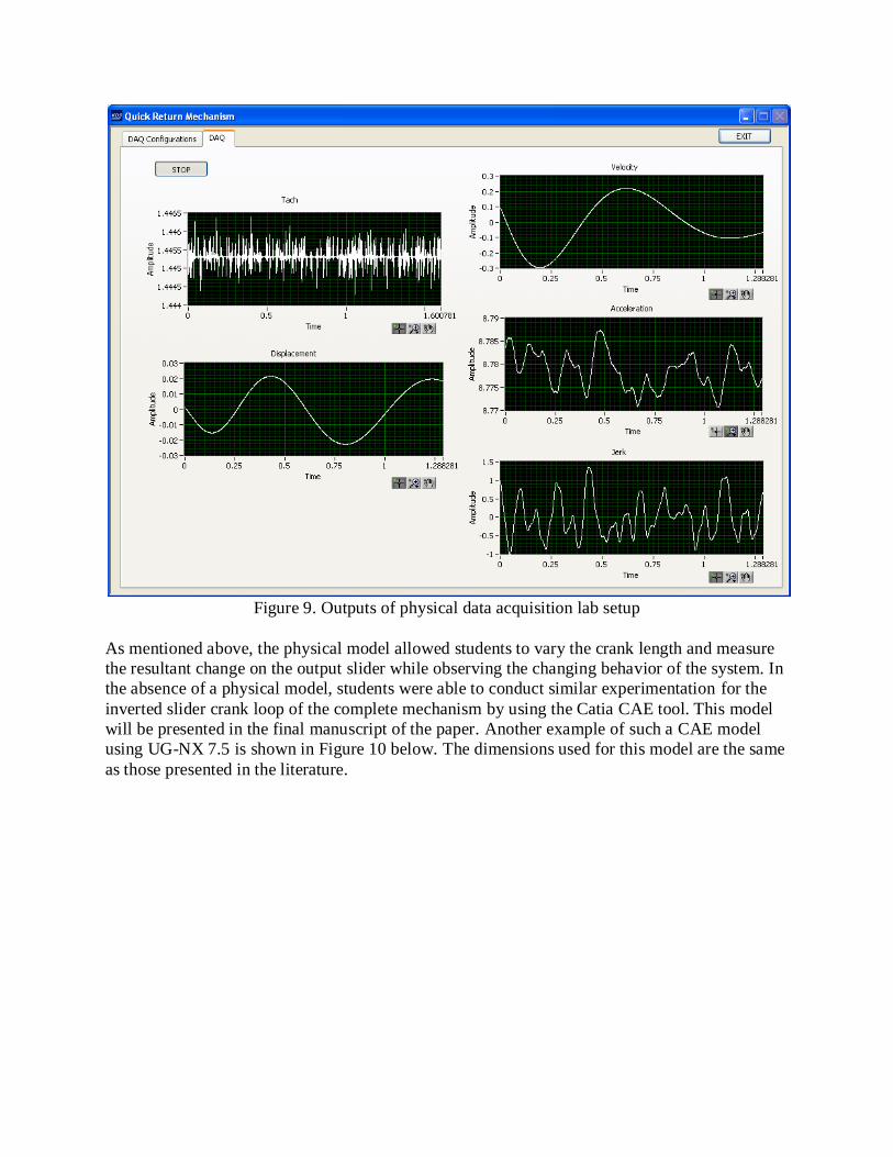
Figure 9. Outputs of physical data acquisition lab setup

As mentioned above, the physical model allowed students to vary the crank length and measure

the resultant change on the output slider while observing the changing behavior of the system. In

the absence of a physical model, students were able to conduct similar experimentation for the

inverted slider crank loop of the complete mechanism by using the Catia CAE tool. This model

will be presented in the final manuscript of the paper. Another example of such a CAE model

using UG-NX 7.5 is shown in Figure 10 below. The dimensions used for this model are the same

as those presented in the literature.

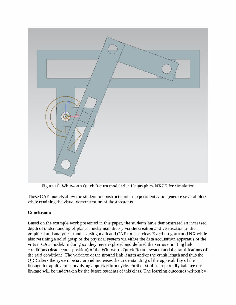
Figure 10. Whitworth Quick Return modeled in Unigraphics NX7.5 for simulation

These CAE models allow the student to construct similar experiments and generate several plots

while retaining the visual demonstration of the apparatus.

Conclusion:

Based on the example work presented in this paper, the students have demonstrated an increased

depth of understanding of planar mechanism theory via the creation and verification of their

graphical and analytical models using math and CAE tools such as Excel program and NX while

also retaining a solid grasp of the physical system via either the data acquisition apparatus or the

virtual CAE model. In doing so, they have explored and defined the various limiting link

conditions (dead center position) of the Whitworth Quick Return system and the ramifications of

the said conditions. The variance of the ground link length and/or the crank length and thus the

QRR alters the system behavior and increases the understanding of the applicability of the

linkage for applications involving a quick return cycle. Further studies to partially balance the

linkage will be undertaken by the future students of this class. The learning outcomes written by

the students indicate that they learned the theory well when complimented with use of a

simulation tool such as a CAE or a MATH tool. Further, they appreciated the use of a real

experimental apparatus, which enabled them to understand better the measurement system and

their limitations based on a comparison of the theoretical and experimental results.

Although in this paper only a quick return mechanism is presented, other planar mechanisms

using higher pairs (cams and gears) are also studied using both graphical and analytical methods,

as well as, analysis using a simulation tool such as UG-NX. Integration of all the learning tools

enable the students to learn better and just in time. The assessment tools used were the

homework, laboratory reports and a comprehensive examination covering all aspects of planar

mechanisms.

Bibliography

1. Catia Version 5 released in 2012 by Dassault Systems.

2. UG-NX Version 8.5 released in 2012 by Siemens.

3. HyperWorks Version 8.0 released in 2006 by Altair Engineering.

4. NX-IDEAS Version 12 released in 2001 by Siemens.

5. SolidWorks 2012 released in 2012 by Dassault Systems.

6. MapleSim Version 6 released in 2012 by Maplesoft.

7. MatLab Version 2012b released in 2012 by Mathworks.

8. C++11 released in 2011 by ISO.

9. Fortran 2008 released in 2010 by IBM.

10. T-K Solver released in 1982 by Software Arts.

11. Campbell, M. & Nestinger S., 2004. Computer-Aided Design and Analysis of the Whitworth Quick Return

Mechanism. Published by the University of California.

12. Norton, R. 2010. Design of Machinery: An Introduction to the Synthesis and Analysis of Mechanisms and

Machines. Published by McGraw-Hill.

13. Erdman A., Sandor G., and Kota S. 2001. Mechanism Design: Analysis and Synthesis. Published by

Prentice Hall.

14. Budynas, R. & Nisbett K. 2011. Shigley’s Mechanical Engineering Design. Published by Tata McGraw

Hill Education.