1

BONNET N. Artificial intelligence and pattern recognition techniques in microscope image processing and analysis.

Advances in Imaging and Electron Physics. (2000) 114, 1-77

Artificial intelligence and pattern recognition techniques in microscope image processing and analysis

Noël Bonnet

INSERM Unit 514 (IFR 53 "Biomolecules") and LERI (University of Reims)

45, rue Cognacq Jay. 51092 Reims Cedex, France. Tel: 33-3-26-78-77-71 Fax: 33-3-26-06-58-61

E-mail: noel.bonnet@univ-reims.fr

Table of contents

I. Introduction II: An overview of available tools originating from the pattern recognition and artificial intelligence culture A. Dimensionality reduction 1. Linear methods for dimensionality reduction 2. Nonlinear methods for dimensionality reduction

3. Methods for checking the quality of a mapping and the optimal dimension of the reduced parameter space

B. Automatic classification 1. Tools for supervised classification 2. Tools for unsupervised automatic classification (UAC) C. Other pattern recognition techniques

1. Detection of geometric primitives by the Hough transform 2. Texture and fractal pattern recognition 3. Image comparison

D. Data fusion III: Applications

A. Classification of pixels (segmentation of multi-component images 1. Examples of supervised multi-component image segmentation 2. Examples of unsupervised multi-component image analysis and

segmentation B. Classification of images or sub-images 1. Classification of 2D views of macromolecules 2. Classification of unit cells of crystalline specimens C. Classification of "objects" detected in images (pattern recognition) D. Application of other pattern recognition techniques 1. Hough transformation

2

2. Fractal analysis 3. Image comparison 4. Hologram reconstruction E. Data fusion IV. Conclusion Acknowledgements References

3

I : Introduction

Image processing and analysis play an important and increasing role in microscope imaging. The tools used for this purpose originate from different disciplines. Many of them are the extensions of tools developed in the context of one-dimensional signal processing to image analysis. The signal theory furnished most of the techniques related to the filtering approaches, where the frequency content of the image is modified to suit a chosen purpose. Image processing is, in general, linear in this context. On the other hand, many nonlinear tools have also been suggested and widely used. The mathematical morphology approach, for instance, is often used for image processing, using gray level mathematical morphology, as well as for image analysis, using binary mathematical morphology. These two classes of approaches, although originating from two different sources, have interestingly been unified recently within the theory of image algebra (Ritter, 1990; Davidson, 1993; Hawkes, 1993, 1995).

In this article, I adopt another point of view. I try to investigate the role already played (or that could be played) by tools originating from the field of artificial intelligence. Of course, it could be argued that the whole activity of digital image processing represents the application of artificial intelligence to imaging, in contrast with image decoding by the human brain. However, I will maintain throughout this paper that artificial intelligence is something specific and provides, when applied to images, a group of methods somewhat different from those mentioned above. I would say that they have a different flavor. People who feel comfortable in working with tools originating from the signal processing culture or the mathematical morphology culture do not generally feel comfortable with methods originating from the artificial intelligence culture, and vice versa. The same is true for techniques inspired by the pattern recognition activity.

In addition, I will also try to evaluate whether or not tools originating from pattern recognition and artificial intelligence have diffused within the community of microscopists. If not, it seems useful to ask the question whether the future application of such methods could bring something new to microscope image processing and if some unsolved problems could take advantage of this introduction.

The remaining paper is divided into two parts. The first part (section II) consists of a (classified) overview of methods available for image processing and analysis in the framework of pattern recognition and artificial intelligence. Although I do not pretend to have discovered something really new, I will try to give a personal presentation and classification of the different tools already available. Then, the second part (section III) will be devoted to the application of the methods described in the first part to problems encountered in microscope image processing. This second part will be concerned with applications which have already started as well as potential applications.

II: An overview of available tools originating from the pattern recognition and artificial intelligence culture

The aim of Artificial Intelligence (AI) is to stimulate the developments of computer algorithms able to perform the same tasks that are carried out by human intelligence. Some fields of application of AI are automatic problem solving, methods for knowledge representation and knowledge engineering, for machine vision and pattern recognition, for artificial learning, automatic programming, the theory of games, etc (Winston, 1977). Of course, the limits of AI are not perfectly well defined, and are still changing with time. AI techniques are not completely disconnected from other, simply computational, techniques, such as data analysis, for instance. As a consequence, the list of topics included in

4

this review is somewhat arbitrary. I chose to include the following ones: dimensionality reduction, supervised and unsupervised automatic classification, neural networks, data fusion, expert systems, fuzzy logic, image understanding, object recognition, learning, image comparison, texture and fractals. On the other hand, some topics have not been included, although they have some relationships with artificial intelligence and pattern recognition. It is the case, for instance, of methods related to the information theory, to experimental design, to microscope automation and to multi-agents system. The topics I have chosen are not independent of each other and the order of their presentation is thus rather arbitrary. Some of them will be discussed in the course of the presentation of the different methods. The rest will be discussed at the end of this section. For each of the topics mentioned above, my aim is not to cover the whole subject (a complete book would not be sufficient), but to give the unfamiliar reader the flavor of the subject, that is to say, to expose it qualitatively. Equations and algorithms will be given only when I feel they can help to explain the method. Otherwise, references will be given to literature where the interested reader can find the necessary formulas. A. Dimensionality reduction The objects we have to deal with in digital imaging may be very diverse: they can be pixels (as in image segmentation, for instance), complete images (as in image classification) or parts (regions) of images. In any case, an object is characterized by a given number of attributes. The number of these attributes may also be very diverse, ranging from one (the gray level of a pixel, for instance) to a huge number (4096 for a 64x64 pixels image, for instance). This number of attributes represents the original (or apparent) dimensionality of the problem at hand, that I will call D. Note that this value is sometimes imposed by experimental considerations (how many features are collected for the object of interest), but is also sometimes fixed by the user, in the case the attributes are computed after the image is recorded and the objects extracted; think of the description of the boundary of a particle, for instance. Saying that a pattern recognition problem is of dimensionality D means that the patterns (or objects) are described by D attributes, or features. It also means that we have to deal with objects represented in a D-dimensional space. A “common sense” idea is that working with spaces of high dimensionality is easier because patterns are better described and it is thus easier to recognize them and to differentiate them. However, this is not necessarily true because working in a space with high dimensionality also has some drawbacks. First, one cannot see the position of objects in a space of dimension greater than 3. Second, the parameter space (or feature space) is then very sparse, i.e. the density of objects in that kind of space is low. Third, as the dimension of the feature space increases, the object description becomes necessarily redundant. Fourth, the efficiency of classifiers starts to decrease when the dimensionality of the space is higher than an optimum (this fact is called the curse of dimensionality). For these different reasons which are interrelated, reducing the dimensionality of the problem is often a requisite. This means mapping the original (or apparent) parameter space onto a space with a lower dimension (ℜD→ℜD’; D’<D). Of course, this has to be done without losing information, which means removing redundancy and noise as much as possible, without discarding useful information. For this, it would be fine if the intrinsic dimensionality of the problem (that is, the size of the subspace which contains the data, which differs from the apparent dimensionality) could be estimated. Since very few tools are available (at the present time) for estimating the intrinsic dimensionality reliably, I will consider that mapping is performed using trial-and-error methods and the correct mapping (corresponding to the true dimensionality) is selected from the outcome of these trials.

5

Many approaches have been investigated for performing this mapping onto a subspace (Becker and Plumbey, 1996). Some of them consist of feature (or attribute) selection. Others consist in computing a reduced set of features out of the original ones. Feature selection is in general very application-dependent. As a simple example, just consider the characterization of the shape of an object. Instead of keeping as descriptors all the contour points, it would be better to retain only the points with high curvature, because it is well known that they contain more significant information than points of low curvature. They are also stable in the scale-space configuration. I will concentrate on feature reduction. Some of the methods for doing this are linear, while others are not. 1. Linear methods for dimensionality reduction Most of the methods used so far for performing dimensionality reduction belong to the category of Multivariate Statistical Analysis (MSA) (Lebart et al., 1984). They have been used a lot in electron microscopy and microanalysis, after their introduction at the beginning of the eighties, by Frank and Van Heel (Van Heel and Frank, 1980, 1981; Frank and Van Heel, 1982) for biological applications and by Burge et al. (1982) for applications in material sciences. The overall principle of MSA consists in finding principal directions in the feature space and to map the original data set onto these new axes of representation. The principal directions are such that a certain measure of information is maximized. According to the chosen measure of information (variance, correlation, etc.), several variants of MSA are obtained such as Principal Components Analysis (PCA), Karhunen Loëve Analysis (KLA), Correspondence Analysis (CA). In addition, the different directions of the new subspace are orthogonal. Since MSA has become a traditional tool, I will not develop its description in this context; see references above and Trebbia and Bonnet (1990) for applications in microanalysis. At this stage, I would just like to illustrate the possibilities of MSA through a single example. This example, which I will use in different places throughout this part of the paper for the purpose of illustrating the methods, concerns the classification of images contained in a set; see section III.B for real applications to the classification of macromolecule images. The image set is constituted of thirty simulated images of a “face”. These images form three classes with unequal populations, with five images in class 1, ten images in class 2 and fifteen images in class 3. They differ by the gray levels of the “mouth”, the “nose” and the “eyes”. Some within-class variability was also introduced, and noise was added. The classes were made rather different, so that the problem at hand can be considered as much easier to solve than real applications. Nine (out of thirty) images are reproduced in Figure 1. Some of the results of MSA (more precisely, Correspondence Analysis) are displayed in Figure 2. Figure 2a displays the first three eigenimages, i.e. the basic sources of information which compose the data set. These factors represent 30%, 9% and 6% of the total variance, respectively. Figure 2b represents the scores of the thirty original images onto the first two factorial axes. Together, these two representations can be used to interpret the original data set: eigen-images help to explain the sources of information (i.e. of variability) in the data set (in this case, “nose”, “mouth” and “eyes”) and the scores allow us to see which objects are similar or dissimilar. In this case, the grouping into three classes (and their respective populations) is made evident through the scores on two factorial axes only. Of course, the situation is not always as simple because of more factorial axes containing information, overlapping clusters, etc. But linear mapping by MSA is always useful. One advantage of linearity is that once sources of information (i.e. eigenvectors of the variance-covariance matrix decomposition) are identified, it is possible to discard

6

uninteresting ones (representing essentially noise, for instance) and to reconstitute a cleaned data set (Bretaudière and Frank, 1988). I would just like to comment on the fact that getting orthogonal directions is not necessarily a good thing, because sources of information are not necessarily (and often are not) orthogonal. Thus, if one wants to quantify the true sources of information in a data set, one has to move from orthogonal, abstract, analysis to oblique analysis (Malinowski and Howery, 1980). Although these things are starting to be considered seriously in spectroscopy (Bonnet et al., 1999a), the same is not true in microscope imaging except as reported by Kahn and collaborators, see section III.A, who introduced the method that was developed by their group for medical nuclear imaging in confocal microscopy studies. 2. Nonlinear methods for dimensionality reduction Many trials to perform dimensionality reduction more efficiently than with MSA have been attempted. Getting a better result requires the introduction of nonlinearity. In this section, I will describe heuristics and methods based on the minimization of a distortion measure, as well as neural-networks based approaches. a. Heuristics: The idea here is to map a D-dimensional data set onto a 2-dimensional parameter space. This reduction to two dimensions is very useful because the whole data set can thus be visualized easily through the scatterplot technique. One way to map a D-space onto a 2-space is to “look” at the data set from two observation positions and to code what is “seen” by the two observers. In Bonnet et al. (1995b), we described a method where observers are placed at corners of the D-dimensional hyperspace and the Euclidean distance from an observer and data points is coded as the information “seen” by the observer. Then, the coded information “seen” by two such observers is used to build a scatterplot.

From this type of method, one can get an idea of the maximal number of clusters present in the data set. But no objective criterion was devised to select the best pairs of observers, i.e. those which preserve the information maximally. More recently, we suggested a method for improving this technique (Bonnet et al., in preparation), in the sense that observers are automatically moved around the hyperspace defined by the data set in such a way that a quality criterion is optimized. This criterion can be either the type of criterion defined in the next section or the entropy of the scatterplot, for instance. b. Methods based on the minimization of a distortion measure Considering that, in a pattern recognition context, distances between objects constitute one of the main sources of information in a data set, the sum of the differences between inter-object distances (before and after nonlinear mapping) can be used as a distortion measure. This criterion can thus be retained to define a strategy for minimum distortion mapping. This strategy has been suggested by psychologists a long time ago (Kruskal, 1964; Shepard, 1966; Sammon, 1969). Several variants of such criteria have been suggested. Kruskal introduced the following criterion in his Multidimensional Scaling (MDS) method: ( )2∑∑

<

−=i ij

ijijMDS dDE (1)

where Dij is the distance between objects i and j in the original feature space and dij is the distance between the same objects in the reduced space. Sammon (1969) introduced the relative criterion instead:

7

∑∑<

−=i ij

DdD

S ij

ijijE2)(

(2)

Once a criterion is chosen, the way to arrive at the minimum, thus performing optimal mapping, is to move the objects in the output space (i.e. changing their coordinates x ) according to some variant of the steepest gradient method, for instance. As an example, the minimization of Sammon’s criterion can be obtained according to the Newton’s method as:

BAxx tt .1 α+=+ (3)

where )(. jlil

j ijij

ijij

il

S xxdDdD

xEA −

−−=

∂∂

= ∑

( )

−+

−−−−=

∂∂

= ∑ij

ijij

ij

jlilijij

j ijijil

S

ddD

dxx

dDdDx

EB 1.1 2

2

2

and t is the iteration index.

It should be stressed that the algorithmic complexity of these minimization processes is very high, since N2 distances (where N is the number of objects) have to be computed each time an object is moved in the output space. Thus, faster procedures have to be explored when the data set is composed of many objects. Some examples of improving the speed of such mapping procedures are:

- selecting (randomly or not) a subset of the data set, performing the mapping of these prototypes, and calculating the projections of the other objects after convergence, according to their original position with respect to the prototypes

- modifying the mapping algorithm in such a way that all objects (instead of only one) are moved in each iteration of the minimization process (Demartines, 1994).

Other methods

Besides the distortion minimization methods and the heuristic approaches described above, several artificial neural-networks approaches have also been suggested. The Self-Organizing Mapping (SOM) method (Kohonen) and the Auto-Associative Neural Network (AANN) method are most commonly used in this context.

c. SOM Self-organizing maps are a kind of artificial neural network which are supposed to reproduce some parts of the human visual or olfactive systems, where input signals are self-organized in some regions of the brain. The algorithm works as follows (Kohonen, 1989):

- a grid of reduced dimension (two in most cases, sometimes one or three) is created, with a given topology of interconnected neurons (the neurons are the nodes of the grid and are connected to their neighbors, see Figure 3),

- each neuron is associated with a D-dimensional feature vector, or prototype, or code vector (of the same dimension as the input data),

- when an input vector xk is presented to the network, the closest neuron (the one whose associated feature vector is at the smallest Euclidean distance) is searched and found: it is called the winner,

- the winner and its neighbors are updated in such a way that the associated feature vectors υi come closer to the input:

υi,t+1 = υi,t + αt . (xk - υi,t) i∈ηt (4)

8

where αt is a coefficient decreasing with the iteration index t, ηt is a neighborhood, also decreasing in size with t.

This process constitutes a kind of unsupervised learning called competitive learning. It results in a nonlinear mapping of a D-dimensional data set onto a D’-dimensional space: objects can now be described by the coordinates of the winner on the map. It possesses the property of topological preservation: similar objects are mapped either to the same neuron or to close-by neurons. When the mapping is performed, several tools can be used for visualizing and interpreting the results:

- the map can be displayed with indicators proportional to the number of objects mapped per neuron,

- the average Euclidean distance between a neuron and its four or eight neighbors can be displayed, to identify clusters of similar neurons,

- the maximum distance can be used instead (Kraaijveld et al., 1995)

An illustration of self-organizing mapping, performed on the thirty simulated images described above, is given in Figure 4. SOM has many attractive properties but also some drawbacks which will be discussed in a later section. Ideally, the dimensionality (1, 2, 3, …) of the grid should be chosen according to the intrinsic dimensionality of the data set, but this is often not the way it is done. Instead, some tricks are used, such as hierarchical SOM (Bhandarkar et al., 1997) or nonlinear SOM (Zheng et al., 1997), for instance.

d. AANN: The aim of auto-associative neural-networks is to find a representation of a data set in a space of low dimension, without losing much information. The idea is to check whether the original data set can be reconstituted once it has been mapped (Baldi and Hornik, 1989; Kramer, 1991). The architecture of the network is displayed in Figure 5. The network is composed of five layers. The first and the fifth layers (input and output layers) are identical, and composed of D neurons, where D is the number of components of the feature vector. The third layer (called the bottleneck layer) is composed of D’ neurons, where D’ is the number of components anticipated for the reduced space. The second and fourth layers (called the coding and decoding layers) contain a number of neurons intermediate between D and D’. Their aim is to compress (and decompress) the information before (after) the final mapping. It has been shown that their presence is necessary. Due to the shape of the network, it is sometimes called the Diabolo network. The principle of the artificial neural network is the following: when an input is presented, the information is carried through the whole network (according to the weight of each neuron) until it reaches the output layer. There, the output data should be as close to the input data as possible. Since this is not the case at the beginning of the training phase, the error (squared difference between input and output data) is back-propagated from the output layer to the input layer. Error back-propagation will be described a little bit more precisely in the section devoted to multi-layer feed-forward neural networks. Thus, the neuron weights are updated in such a way that the output data more closely resembles the input data. After convergence, the weights of the neurons are such that a correct mapping of the original (D-dimensional) data set can be performed on the bottleneck layer (D’-dimensional). Of course, this can be done without too much loss of information only if the chosen dimension D’ is compatible with the intrinsic dimensionality of the data set.

9

e. Other dimensionality reduction approaches In the previous paragraphs, the dimensionality reduction problem was approached by abstract mathematical techniques. When the "objects" considered have specific properties, it is possible to envisage (and even to recommend) how to exploit these properties for performing dimensionality reduction. One example of this approach consists in replacing images of centro-symmetric particles by their rotational power spectrum (Crowther and Amos, 1971): the image is split into angular sectors, the summed signal intensity within the sectors is then Fourier transformed to give a one-dimensional signal containing the useful information related to the rotational symmetry of the particles.

3. Methods for checking the quality of a mapping and the optimal dimension of

the reduced parameter space Checking the quality of a mapping for selecting one mapping method over others is

not an easy task and depends on the criterion chosen to evaluate the quality. Suppose, for instance, that the mapping is performed through an iterative method aimed at minimizing a distortion measure e.g. as MDS or Sammon’s mappings do. If the quality criterion chosen is the same distortion measure, this method will be found to be good, but the same result may not be true if other quality criteria are chosen. Thus, one has sometimes to evaluate the quality of the mapping through the evaluation of a subsidiary task, such as classification of known objects after dimensionality reduction (see for instance De Baker et al. 1998).

Checking the quality of the mapping may also be a way to estimate the intrinsic (or true) dimensionality of the data set, that is to say the optimum reduced dimension (D’) for the mapping, or in other words the smallest dimension of the reduced space for which most of the original information is preserved.

One useful tool for doing this (and checking the different results visually) is to draw the scatterplot relating the new inter-distances (dij) to the original ones (Dij). While most information is preserved, the scatterplot display remains concentrated along the first diagonal (dij≈Dij ∀i ∀j). On the other hand, when some information is lost because of excessive dimensionality reduction, the scatterplot is no longer concentrated along the first diagonal, and distortion concerning either small distances or large distances (or both) becomes apparent.

Besides visual assessment, the distortion can be quantified through several descriptors of the scatterplot, such as:

- contrast: ( ) ( )ijiji ij

ijij dDpdDDC ,.)'( 2∑∑<

−= (5)

- entropy: ( ) ( )[ ]ijijijiji ij

dDpdDpDE ,log.,)'( ∑∑<

= (6)

where p(Dij,dij) is the probability that the original and post-mapping distances between objects i and j take the values Dij and dij, respectively. Plotting C(D’) or E(D’) as a function of the reduced dimensionality D’ allows us to check the behavior of the data mapping. A rapid increase in C or E when D’ decreases is often the sign of an excessive reduction in the dimensionality of the reduced space. The optimality of the mapping can be estimated as an extremum of the derivative of one of these criteria. Figure 6 illustrates the process described above. The data set composed of the thirty simulated images was mapped onto spaces of dimension 4, 3, 2 and 1, according to Sammon’s mapping. The scatterplots relating the distances in the reduced space to the original distances are displayed in Figure 6a. One can see that a large change occurs for D’=1, indicating that

10

this is too large a dimensionality reduction. This visual impression is confirmed by Figure 6b, which displays the behavior of the Sammon criterion for D’ varying from 4 to 1. These tools may be used whatever the method used for mapping including MSA and neural networks. According to the results obtained by De Baker et al. (1998), nonlinear methods provide better results than linear methods for the purpose of dimensionality reduction. Event covering

Another topic connected to the discussion above concerns the interpretation of the different axes of representation after performing linear or nonlinear mapping. This interpretation of axes in terms of sources of information is not always an easy task. Harauz and Chiu (1991, 1993) suggested the use of the event-covering method, based on hierarchical maximum entropy discretization of the reduced feature space. They showed that this probabilistic inference method can be used to choose the best components upon which to base a clustering, or to appropriately weight the factorial coordinates to under-emphasize redundant ones. B. Automatic classification Even when they are not perceived as such, many problems in intelligent image processing are, in fact, classification problems. Image segmentation, for instance, be it univariate or multivariate, consists in the classification of pixels, either into different classes representing different regions, or into boundary/non-boundary pixels. Automatic classification is one of the most important problems in artificial intelligence and covers many of the other topics in this category such as expert systems, fuzzy logic and some neural networks, for instance. Traditionally, automatic classification has been subdivided into two very different classes of activity, namely supervised classification and unsupervised classification. The former is done under the control of a supervisor or a trainer. The supervisor is an expert in the field of application who furnishes a training set, that is to say a set of known prototypes for each class, from which the system must be able to learn how to move from the parameter (or feature) space to the decision space. Once the training phase is completed (which can generally be done if and only if the training set is consistent and complete), the same procedure can be followed for unknown objects and a decision can be made to classify them into one of the existing classes or into a reject class. In contrast, unsupervised automatic classification (also called clustering) does not make use of a training set. The classification is attempted on the basis of the data set itself, assuming that clusters of similar objects exist (principle of internal cohesion), and that boundaries can be found which enclose clusters of similar objects and disclose clusters of dissimilar objects (principle of external isolation). 1. Tools for supervised classification Tools available for performing supervised automatic classification are numerous. They include interactive tools and automatic tools. One method in the first group is Interactive Correlation Partitioning (ICP). It can be decomposed into four steps. The first one consists in mapping the data set on a two- or three-dimensional parameter space. Of course, if objects to classify are already described by two or three features only, this step is unnecessary. Then, a two- or three-dimensional scatterplot is drawn from the two or three features (Jeanguillaume, 1985; Browning et al., 1987; Bright et al, 1988; Bright and Newbury, 1991; Kenny et al.,

11

1994). If objects form classes, the scatterplot displays clusters of points, more or less well separated. Thus, the third step consists, for the user, in designating interactively (with the computer mouse), the boundaries of the classes he/she wants to define. Finally, a back-mapping procedure can be used to label the original objects according to the different classes defined in the feature space. Figure 7 illustrates the use of three-dimensional scatterplots for the analysis of series of three Auger images. One of the aims of artificial intelligence techniques in this context is to move from ICP to Automatic Correlation Partitioning (ACP), i.e. to automate the process of finding clusters of similar objects in the original or reduced parameter space. Automatic tools include:

- the estimation of a probability density function (pdf) for each class of the training set, by the Parzen technique for instance, followed by the application of the Bayes theorem. The Parzen technique consists in smoothing the point distribution (of objects in the parameter space) by summing up the contributions of smooth kernels centered on the positions of each object. The Bayes theorem (originating from the maximum likelihood decision theory) states that one unknown object should be classified in the class for which the probability density function (at the object position) is maximum.

- the k nearest neighbors (kNN) technique, where unknown objects are classified according to the class their neighbors in the training set belong to (voting rule),

- the technique of discriminant functions in which linear or nonlinear boundaries between the different classes in the parameter space are estimated on the basis of the training set. Then, unknown objects are classified according to their position relative to the boundaries.

These classical tools are described in many textbooks (Fukunaga, 1972; Duda and Hart, 1973) and will not be repeated here. I will rather concentrate on less-known methods pertaining more to artificial intelligence than to classical statistics. a. Neural networks: Neural networks were invented at the end of the nineteen-forties for the purpose of performing supervised tasks in general (and automatic classification in particular) more efficiently than classical statistical methods were able to do. The aim was to try to reproduce the capabilities of the human brain in terms of learning and generalization. For this purpose, several ingredients were incorporated into the recipe such as non linearities on the one hand and multi-level processing on the other (Lippmann, 1987; Zupan and Gasteiger, 1993; Jain et al., 1996). Although many variants of neural networks have been developed for supervised classification, I will concentrate on three of them: the multi-layer feed-forward neural networks (MLFFNN), the radial basis functions neural networks (RBFNN) and neural networks based on the adaptive resonance theory (ARTNN). Multi-layer feed-forward networks are by far the most frquently used neural networks in a supervised context. A schematic architecture is displayed in Figure 8. The working scheme of the network is the following (the corresponding formulas can be found in references listed above): during the training step, objects (represented by D-feature vectors) are fed into the network at the input layer composed of D neurons. The feature values are propagated through the network in the forward direction; hence the name of 'feed-forward' networks. The output of each neuron in the intermediate (or hidden) and output layers is computed according to the neuron coefficients (or weights) and to the chosen nonlinear

12

activation function. At the output layer, an output vector is obtained. Two situations can occur -either the output vector corresponds to the expected output (the training set is characterized by a known output, a class label or something equivalent) or it does not. In the former case, the neuron coefficients of the whole network are left unmodified and the process is repeated with a new sample of the training set. In the latter case, the neuron coefficients of the whole network are modified through a back-propagation procedure: the error (difference between the actual output and the expected output) is propagated from the output layer towards the input layer. The neuron weights are modified in such a way that the error is minimized i.e. the first derivative of the error against the neuron weight is set to zero. First, the coefficients associated with neurons in the output layers are modified. Then, coefficients of neurons in the hidden layers(s) are also modified. The process of presentation of samples from the training set is repeated until learning is completed i.e. convergence of the neuron coefficients to stable values and minimization of the output error for the whole training set is achieved. Then, the application of the trained neural network to the unknown data set may start; the neural architecture, if properly chosen, is supposed to be able to generalize to new data. Although such neural networks have been considered as black boxes for a long time, there are now several tools available for understanding their behavior in real situations, for modifying (almost automatically) their architecture i.e. number of hidden layers, number of neurons per layer, etc. (Hoekstra and Duin, 1997; Tickle et al., 1998). Another type of neural network devoted to supervised classification is the radial basis functions (RBF) neural networks. As MLFFNN networks, RBF networks have a multi-layer architecture but with only one hidden layer. Their aim is to establish models of the different classes which constitute a learning set. More specifically, an RBF network works as a kind of function estimation method. It approximates an unknown function (a probability density function, for instance) as the weighted sum of different kernel functions, the so-called radial basis functions (RBF). These RBF functions are used in the hidden layer in the following way: each node (i=1 … K) in the hidden layer represents a point in the parameter space, characterized by its coordinates (cij, j=1 … N). When an object (x) serves as input to the first layer, its Euclidean distances to all nodes of the hidden layer are computed using:

( )∑=

−=N

jijji cxd

1

2 (7)

and the output of the network is computed as:

)(.)(1

0 i

K

ii daaxoutput Φ+= ∑

=

(8)

where )(uΦ is the RBF, chosen to be (for instance):

)exp()( 2

2

σuu −=Φ (9)

or )exp(

1)(

2

2

σuR

Ru+

+=Φ (10)

where σ and R are adjustable parameters. The training of such a network is also made by gradient descent through back-propagation: an error function is defined, as the distance between the output value and the target value, and minimized. Through the iterative minimization process, the network parameters (centers of classes ci, weights ai, R, σ) are updated. Then, unknown objects can be processed.

13

b. Expert systems An expert system is a computer program supposed able to perform tasks ordinarily performed by human experts, especially in domains where relationships may be inexact and conclusions are uncertain. Expert systems are also based on training (on the basis of a training set composed of objects and the associated decision marks). An expert system is composed of three separated entities: the knowledge base, the inference engine and the available data. The knowledge base includes specific knowledge (or assumptions) concerning the domain of application. The inference engine is a set of mechanisms that use the knowledge base to control the system and solve the problem at hand. There are several variants of expert systems. The mostly used are rule-based expert systems. For expert systems in this category, the knowledge base is in the form of If-Then rules. For instance, rules may associate a combination of feature intervals to one decision outcome:

“If feature A is … and feature B is … Then decision is ….”. There are several ways to get the rules out of the training set (Buchanan ans Shortliffe, 1985; Jackson, 1986). It should be noted that the values of features incorporated into the rules are not necessarily feature intervals. The development of several variants of multi-valued logic has rendered things more flexible. For instance, the fuzzy sets theory, the possibility theory or the evidence theory can be used in this context.

The fuzzy set theory was introduced by Zadeh (1965) as a new way to represent a continuum of values at the output rather than the usual binary output of traditional binary logic and thus accommodate vagueness, ambiguity and imprecision. These concepts are usually described in a non-statistical way, in contrast to what happens with the probability theory. Objects are characterized by their membership (measured by membership values) of the different classes of the universe, which represent similarity of objects with imprecisely defined properties of these classes. The membership function values µki lie between 0 and 1 and are also characterized by their sum equal to one:

11

=∑=

C

ikiµ ∀k=1…N ()

where C is the number of classes. The possibility theory (Dubois and Prade, 1985) does not impose such a constraint, but

only:

NN

kki << ∑

=10 µ ∀i=1…C ()

The membership values thus represent a degree of typicality rather than a degree of sharing. In addition, the concept of necessity is also used. The evidence theory, also called the Dempster-Shafer theory (Shafer, 1976), allows also to represent both uncertainty and imprecision in a more flexible way than the Bayes theory. Each event A is characterized by a mass function, from which two higher level functions can be defined, plausibility (maximum uncertainty) and belief (minimum uncertainty). Then, possibilities are provided to combine the measures of evidence from different sources. It should also be stressed that the neural network and expert system approaches may not be completely independent (Bezdek, 1993). Possibilities have been developed for deducing expert system rules from a MLFFNN-based system (Mitra and Pal, 1996; Huang and Endsley, 1997), and for deducing the architecture of a neural network on the basis of rules obtained after an expert system procedure (Yager, 1992).

14

2. Tools for unsupervised automatic classification (UAC)

Clustering (a synonym of UAC) has also been the subject of a lot of work (Duda and Hart, 1973; Fukunaga, 1972). The main difference with supervised classification is that, with a few exceptions, most of the available methods rely on classical statistics, namely the consideration of the probability density functions. Another difference is that, in contrast with supervised approaches, the number of classes is often unknown in clustering problems, and has also to be estimated. Clustering methods can be subdivided into two main groups: hierarchical and partitioning methods. Methods from the former group build ascendant or descendant hierarchies of classes, while methods from the latter group divide the object set into mutually exclusive classes.

a. Hierarchical classification methods Hierarchical ascendant classification (HAC) starts from a number of classes equal to

the number of objects in the set. The two closest objects are then grouped to form a class. Then, the two closest classes (which can be composed of one or several objects) are agglomerated and so on. The classification process is stopped when all objects are gathered into one single class. The upper levels of the hierarchical structure can be represented by a dendrogram. The results of the hierarchical classification depends strongly on the choice of the distance used for comparing pairs of classes and selecting the two closest ones, at any stage of the classification process.

The single linkage algorithm corresponds to the definition of the distance as the distance between the two most similar objects:

jij

likji NlNkxxdCCd ...1,...1)),,(min(),( === (13)

where ikx is one of the iN objects belonging to class iC and j

lx is one of the jN objects belonging to class jC .

The complete linkage algorithm corresponds to the definition of distance between classes as the distance between the most dissimilar objects of the class:

jij

likji NlNkxxdCCd ...1,...1)),,(max(),( === (14)

The average linkage algorithm corresponds to the definition of distance between classes as the average distance between pairs of objects belonging to these classes:

),(.1),(

1 1

jl

N

k

N

l

ik

jiji xxd

NNCCd

i j

∑∑= =

= (15)

The centroid linkage algorithm corresponds to the distance between classes defined as the distance between their centers of mass:

),(),( jiji xxdCCd = (16)

where ∑=

=iN

k

ik

i

i xN

x1

1 and ∑=

=jN

l

jl

j

j xN

x1

1

The Ward method (Ward, 1963) is based on a minimization of the total within-class variance at each step of the process. In other words, the pair of clusters which are aggregated are those which lead to the lowest increase in the within-class variance:

[ ]2),(. ji

ji

jiij xxd

NNNN

AIV+

= (17)

Of course, each algorithm possesses its own tendency to produce a specific type of

clustering result. Single linkage produces long chaining clusters and is very sensitive to noise.

15

Complete linkage and the Ward method tend to produce compact clusters of equal size. Average linkage and centroid linkage are capable of producing clusters of unequal size but the total within-class variance is not minimized.

Hierarchical classification methods (including hierarchical ascendant and descendant methods) are often criticized because they suffer from a number of inconveniences:

- they work well for well separated clusters but less well for overlapping clusters, - they have a tendency (except with the single linkage procedure) to produce

hyperspherical clusters, - when the idea of a hierarchical classification is questionable, it is difficult to find

where to cut the dendrogram, - their computation cost is very high. Methods described below are all partitioning methods.

b. The C-means algorithm I will start the discussion with one of the oldest algorithms viz. the C-means algorithm

- often called the K-means algorithm, but the difference is irrelevant. As its name implies, this algorithm uses the concept of mean of class, represented by the center of mass of the class in the feature space. The algorithm consists in iteratively refining the estimation of the C class means and the partitioning of the data objects into the classes (Bonnet, 1995): Algorithm 1: C-means Step 1: Fix the number of classes, C Step 2: Initialize (randomly or not) the C class center coordinates

Step 3: Distribute the N objects to classify into the C classes, according to the nearest neighbor rule:

classxk → i { }ijxxdxxd jk

ik ≠∀< ),(),( (18)

Step 4: Compute the new class means, on the basis of objects belonging to each class:

∑=

=iN

kk

i

i xN

x1

1 (19)

Step 5: If the class centers did not move significantly (compared to the previous cycle), go to step 6, otherwise go to step 3.

Step 6: Modify the number of classes (within limits fixed by the user) and go to step 1. In general, the number of classes is unknown and the algorithm has to be run for a

varying number of classes (C). For each of partitions obtained, a criterion evaluating the quality of the partition has to be computed and the number of classes is chosen according to the extreme of this quality criterion. Of course, several different criteria lead to the same optimum in favorable situations of well separated classes, but not in unfavorable situations of large overlap between classes. A partial list of quality criteria can be found in Bonnet et al. (1997).

c. The fuzzy C-means algorithm The C-means algorithm can be improved within the framework of fuzzy logic, and

becomes the fuzzy C-means (FCM) algorithm in this context (Bezdek, 1981). The main difference is that, at least during the first steps of the iterative approach, objects are allowed to belong to all the classes simultaneously, reflecting the non-stabilized stage of membership. Step 3 and 4 of the previous algorithm are thus replaced by:

Algorithm 2: Fuzzy C-means Step 3’: Compute the degrees of membership of each object k to each class i as:

16

∑

=

j kj

kiki

d

d1

1µ (20)

where dki is the distance between object k and center of class i. Step 4’: Compute the centers of the classes according to the degrees of membership µki:

∑

∑

=

== N

k

mki

N

kk

mki

ix

x

1

1.

µ

µ , i=1…C (21)

where m is a fuzzy coefficient chosen between 1 (for crisp classes) and infinity (for completely fuzzy classes). m is generally chosen equal to 2. In addition, a defuzzification step is added: Step 5: the final classification is obtained by setting each object in the class with the largest degree of membership: Object k → class i {µik>µjk ∀j≠i} Specific criteria have been suggested for estimating the quality of a partition in the context of the fuzzy logic approach. Most of them rely on the quantification of fuzziness of the partition after convergence but before defuzzification (Roubens, 1978; Carazo et al., 1989; Gath and Geva, 1989; Rivera et al., 1990, Bezdek and Pal, 1998). Information theoretical concepts (entropies for instance), can also be used for selecting an optimal number of classes. Several variants of the FCM technique have been suggested, where the fuzzy set theory is replaced by another theory. When the possibility theory is used, for instance, the algorithm becomes the possibilistic C-means (Krishnapuram and Keller, 1993), which has its own advantages but also its drawbacks (Barni et al., 1996; Ahmedou and Bonnet, 1998).

d. Parzen/watersheds The methods described above share an important limitation; they all consider that a class can be conveniently described by its center. It means that hyperspherical clusters are anticipated. Replacing the Euclidean distance by the Mahalanobis distance makes the method more general, because hyperelliptical clusters (with different sizes and orientations) can now be handled. But it also makes the minimization method more susceptible to sink into local minima instead of reaching a global minimum. Several clustering methods have been proposed that do not make assumptions concerning the shape of clusters. As examples, I can cite:

- a method based on "phase transitions" (Rose et al., 1990) - the mode convexity analysis (Postaire and Olejnik, 1994) - the blurring method (Cheng, 1995) - the dynamic approach (Garcia et al., 1995) I will describe in more details the method I have worked on, which I will name the

Parzen/watersheds method. This method is a probabilistic one; clusters are identified in the parameter space as areas of high local density separated by areas of lower object density. The first step of this method consists in mapping the data set to a space of low dimension (D'<4). This can be done with one of the methods described in section II.A. The second step consists in estimating, from the mapped data set, the total probability density function i.e. the pdf of the mixture of classes. It can be done by the Parzen method, originally designed in the

17

supervised context (Parzen, 1962). The point distribution is smoothed by convolution with a kernel:

∑=

−=N

kkxxxpdf

1)ker()( (22)

where ker(x) is a smoothing function chosen from many possible ones (Gaussian, Epanechnikov, Mollifier, etc) and xk is the position of object k in the parameter space. Now, a class is identified by a mode of the estimated pdf. Note that the number of modes (and hence the number of classes) is related to the extension parameter of the kernel -the standard deviation σ in the case of a Gaussian kernel, for instance. This reflects the fact that several possibilities generally exist for the clustering of a data set. We cope with this problem by plotting the curve of the number of modes of the estimated pdf against the extension parameter σ. This plot often displays some plateaus that indicate relative stability of the clustering and offer several possibilities to the user, who has however to make a choice. It should be stressed that, unless automatic methods exist for estimating the smoothing parameter, the results obtained following this method do not often provide consistent results in terms of number of classes (Herbin et al., in preparation).

Once an estimation of the pdf is obtained, the next step consists in segmenting the parameter space into as many regions as there are modes and hence classes. For this purpose, we have chosen to apply tools originating from mathematical morphology. Although these tools were originally developed for working in the image space, the fact that they are based on the set theory makes them easily exptendible to work in any space, like the parameter space involved in automatic classification. In the first version of this work (Herbin et al., 1996), we used the skeleton by influence zones (SKIZ). This tool originates from binary mathematical morphology, and computes the zones of influence of binary objects. Thus, we had to threshold the estimated pdf at different levels (starting from high levels) and deduce the zones of influence of the different parts of the pdf. When arriving at a level of the pdf close to zero, we get the partition of the parameter space into different regions, labeled as the different classes. In the second version of this work (Bonnet et al., 1997; Bonnet, 1998a), we have replaced the SKIZ by the watersheds. This tool originates from gray level mathematical morphology, and was developed mainly for the purpose of image segmentation (Beucher and Meyer, 1992; Beucher, 1992). It can be applied easily to the estimated pdf, in order to split the parameter space (starting from the modes) into as many regions as there are modes.

Once the parameter space is partitioned and labeled, the last (easy) step consists in demapping, i.e. labeling objects according to their position within the parameter space after mapping.

The whole process is illustrated in Figures 9 and 10. In the former case, the classification of images (described above) is attempted. A plateau of the number of modes (as a function of the smoothing parameter) is obtained for three modes. It corresponds to the three classes of images. In the latter case, the classification of pixels (of the same thirty simulated images) is attempted, starting from the scatterplot built on the first two eigenimages obtained after Correspondence Analysis. A plateau of the curve is observed for four modes, that correspond to the four classes of pixels (face and background are classified within the same class, because their gray levels do not vary, eyes, mouth and nose).

e. SOM: SOM was originally designed as a method for mapping (see section II.A.2.c), i.e. dimensionality reduction. However, several attempts have been made to extrapolate its use towards unsupervised automatic classification. One of the possibilities for doing so is to choose a small number of neurons, equal to the number of expected classes. This was done successfully by some authors, including

18

Marabini and Carazo (1994), as will be described in section III.B.1. But this method may be hazardous, because there is no guarantee that objects belonging to one class will all be mapped onto the same neuron, especially when the populations of the different classes are different. Another possibility is thus to choose a number of neurons much higher than the expected number of classes, to fiund some tricks to get the true number of classes and then to group SOM neurons to form homogeneous classes. For the first step, one possibility is to display (for each neuron) the normalized standard-deviation of its distances to its neighbors (Kraaijveld et al., 1995). This shows clusters separated by valleys, from which the number of clusters can be deduced, together with the boundaries between them. One of the theoretical problems associated with this approach is that SOM preserves the topology but not the probability density function. It was shown in Gersho (1979) that the pdf in the D’-dimensional mapping space can be approximated as:

'11

1

)()'( DDpdfDpdf+

= (23) Several attempts (Yin and Allison, 1995; Van Hulle, 1996, 1998) have been made to improve the situation. At this stage, I can also mention that variants of SOM have been suggested to perform not only dimensionality reduction but also clustering. One of them is the Generalized Learning Vector Quantization (GLVQ) algorithm (Pal et al., 1993), also called Generalized Kohonen Clustering Network (GKCN), which consists in updating all prototypes instead of the winner only, and thus results in a combination of local modeling and global modeling of the classes. This algorithm was improved subsequently by Karayiannis et al. (1996). Another one is the Fuzzy Learning Vector Quantization (FLVQ) algorithm (Bezdek and Pal, 1995), also called the Fuzzy Kohonen Clustering Network (FKCN). This algorithm, and several variants of it, can be considered as the integration of the Learning Vector Quantization (LVQ) algorithm, the supervised counterpart of SOM, and of the fuzzy C-means algorithm. A discussion of these and other clustering variants, including those based on the possibility theory, was given in Ahmedou and Bonnet (1998).

f. ART: Another class of neural networks was developed around the Adaptive Resonance

Theory (ART). It is based on the classical concept of correlation (similar objects are highly positively correlated) enriched by the neural concepts of plasticity-stability (Carpenter and Grossberg, 1987). Simply, an ART-based neural network consists of defining as many neurons as necessary to split an object set into several classes such that one neuron represents one class. The network is additionally characterized by a parameter, called the vigilance parameter. When a new object is presented to the network, it is compared to all the already existing neurons. The winner is defined as the neuron closest to the object presented. If a similarity criterion with the winner is higher than the vigilance parameter, the network is said to enter into resonance and the object is attached to the winner’s class. The neuron vector is also updated:

υw ← υw + αt . (xk - υw) (24) If the similarity criterion is lower than the vigilance parameter, a new neuron is created. Its description vector is initialized with the object's feature vector. Several variants of this approach (some of them working in the supervised mode) have been devised (Carpenter et al., 1991, 1992).

19

C. Other pattern recognition techniques Automatic classification (of pixels, of whole images, of image parts) is not the only activity involving pattern recognition techniques. Other applications include: the detection of geometric primitives, the characterization and recognition of textured patterns, etc. Image comparison can also be considered as a pattern recognition activity.

1. Detection of geometric primitives by the Hough transform Simple geometric primitives (lines, segments, circles, ellipses, etc.) are easily recognized by the human visual system when they are present in images, even when they are not completely visible. The task is more difficult in computer vision, because it requires high level procedures (restoration of continuity, for instance) in addition to low level procedures such as edge detection, for instance. One elegant way for solving the problem was invented by Hough (1962) for straight lines, and subsequently generalized to other geometric primitives. The general principle consists in mapping the problem into a parameter space, the space of the possible values for the parameters of the analytical geometric primitive e.g. slope and intercept of a straight line, center coordinates and radius of a circle, etc. Each potentially contributing pixel with a non-null gray level in a binary image is transformed into a parametric curve in the parameter space. For instance, in the case of a straight line: y = a . x + b b = yi – a . xi for a pixel of coordinates (xi, yi) This is called a one-to-many transformation. If several potentially contributing pixels lie on the same straight line in the image space, several lines are obtained in the parameter space. Since the couple (a,b) of parameters is the same for all pixels, these lines intercept at a unique position in the parameter space (a,b), resulting in a many-to-one transformation. A voting procedure (all the contributions in the parameter space are summed up) followed by a peak detection allow depiction of the different (a,b) couples which correspond to real lines in the image space. This procedure was extended, with some modifications, to a large number of geometric primitives: circles, ellipses, polygons, sinusoids, etc (Illingworth and Kittler, 1988). Many methodological improvements have also been made, among which I will just cite:

- the double pass procedure (Gerig, 1987) - the randomized Hough transform (Xu and Oja, 1993) - the fuzzy Hough transform (Han et al., 1994). A few years ago, the Hough transform, originally designed for the detection of

geometrically well-defined primitives, was extended to natural shapes (Samal and Edwards, 1997), characterized by some variability. The idea was to consider a population of similar shapes and to code the variability of the shape through the union and intersection of the corresponding silhouettes. Then, a mapping of the area comprised between the inner and outer shapes allows detection of any shape intermediate between these two extreme shapes. Recently, I showed that the extension to natural shapes does not necessitate that a population of shapes has to be gathered (Bonnet, unpublished). Instead, starting from a unique shape, its variability can be coded either by a binary image (the difference between the dilated and eroded versions of the corresponding silhouette) or by a gray-valued image (taking into account the internal and external distance functions to the silhouette) expressing the fact that the probability of finding the boundary of an object belonging to the same class as the reference decreases when one moves farher from the reference boundary. 2. Texture and fractal pattern recognition

20

Texture is one possible feature which allows us to distinguish different regions in an image, or to differentiate different images. Texture analysis and texture pattern recognition have a long history, starting from the nineteen-seventies. It has been discovered that texture properties have to do with second order statistics and most methods rely on an estimation of these parameters at a local level, from different approaches:

- the gray level co-occurrence matrix, and its secondary descriptors, - the gray level run lengths, - Markov auto-regressive models, - filter banks, and Gabor filters specifically, - wavelets coefficients.

A subclass of textured patterns is composed of fractal patterns. They are characterized by the very specific property of self-similarity, which means that they have a similar appearance when they are observed at different scales of magnification. When this is so, or partly so, the objects (either described by their boundaries or by the gray level distribution of their interior) can be characterized by using the concepts of fractal geometry (Mandelbrot, 1982), and especially the fractal dimension. Many practical methods have been devised for estimating the characteristics (fractal spectrum and fractal dimension) of fractal objects. All these methods are based on the concept of self-similarity of curves and two-dimensional images. A brief list of these methods is given below (the references to these methods can be found in Bonnet et al., 1996):

- the box-counting approach: images are represented as 3D entities (the gray level represents the third dimension). The number N of three-dimensional cubic boxes of size L necessary to cover the whole 3D entity is computed, for different values of L. The fractal dimension is estimated as the negative of the slope of the curve Log(N) versus Log(L).

- the Hurst coefficient approach: the local fractal dimension is estimated as D=3-s, where s is the slope of the curve Log(σ) versus Log(d), where σ is the standard deviation of the gray levels of neighboring pixels situated at a distance d of the reference pixel. This local fractal feature can be used to segment images composed of different regions differing by their fractal dimension.

- the power spectrum approach: the power spectrum of the image (or of sub-images) is computed and averages over concentric rings in the Fourier space with spatial frequency f are obtained. The (possibly) fractal dimension of the 2D image is estimated as D=4-s, where s is the slope of the curve Log(P1/2) versus Log(f), where P is the power at frequency f.

- the mathematical morphology approach, also called the blanket or the cover approach: the image is again represented as a 3D entity. It is dilated and eroded by structuring elements of increasing size r. The equivalent area A enclosed between the dilated and eroded surfaces (or between the dilated and original surfaces, or between the eroded and original surfaces) is computed. The (possibly) fractal dimension is estimated as D=2-s, where s is the slope of the curve Log(A) versus Log(r).

The estimations of the fractal dimension obtained from these different methods are not

strictly equivalent, because they do not all measure the same quantity. But the relative values obtained for different images with the same method can be used to rank these images according to the estimated fractal parameter, which is any case is always a measure of the image complexity.

21

3. Image comparison The comparison of two images can also be considered as a pattern recognition problem. It is involved in several activities:

- image registration is a pre-processing technique often required before other processing tasks can be performed,

- comparison of experimental images to simulated ones is a task more and more involved in High Resolution Electron Microscopy (HREM) studies.

Traditionally, image comparison has been made according to the least squares (LS) criterion, i.e. by minimizing the quantity:

[ ]221 )),((),(∑∑ −

i jjiITjiI (25)

where T is a transformation applied to the second image I2 to make it more similar to the first one I1. This transformation can be a geometrical transformation, a gray level transformation, or a combination of both.

Several variants of the LS criterion have been suggested: - the correlation function (also called the cross-mean):

)),(().,(),( 2121 jiITjiIIICi j

∑∑≈ (26)

or the correlation coefficient:

)(

212121

21.

)(.),(),(

ITI

ITIIICII

σσρ

−= (27)

are often used, especially for image registration (Frank, 1980) - the least mean modulus (LMM) criterion:

∑∑ −≈i j

jiITjiIIILMM )),((),(),( 2121 (28)

is sometimes used instead of the least squares criterion due to its lower sensitivity to noise and outliers (Van Dyck et al., 1988). In the field of single particle HREM, a strong effort has been made for developing procedures which make the image recognition methods invariant against translation and rotation, which is a requisite for the study of macromolecules. For instance, auto-correlation functions (ACF) have been used for performing the rotational alignment of images before their translational alignment (Frank, 1980). Furthermore, the double auto-correlation function (DACF) constitutes an elegant way to perform pattern recognition with translation, rotation and mirror invariance (Schatz and Van Heel, 1990). In addition, self-correlation functions (SCF) and mutual correlation functions (MCF) have been defined (on the basis of the amplitude spectra) to replace the auto-correlation (ACF) and cross-correlation (CCF) functions based on the squared amplitude (Van Heel et al., 1992). There have been also some attempts to consider higher order correlation functions (the triple correlation and the bispectrum) for pattern recognition. Hammel and Kohl (1996) proposed a method to compute the bispectrum of amorphous specimens. Marabini and Carazo (1996) showed that bispectral invariants based on the projection of the bispectrum in lower-dimensional spaces are able to retain most of the good properties of the bispectrum in terms of translational invariance and noise insensitivity, while avoiding some of its most important problems.

22

An interesting discussion concerns the possibility of applying the similarity criteria in the reciprocal space (after Fourier transforming the images) rather than in the real space. Some other useful criteria can also be defined in this frequency space:

- the phase residual (Frank et al., 1981):

∑∑

+

+=∆

21

221

()(FF

FF δθθ (29)

where F1 and F2 are the complex Fourier spectra of images 1 and 2, and δθ is their phase difference. - the Fourier ring correlation (Saxton and Baumeister, 1982; Van Heel and Stöffler-

Meilicke, 1985):

( ) 2/122

21

*21

.

).(

∑ ∑∑=

FF

FFFRC (30)

or

∑∑=

).().(

21

*21

FFFF

FRCX (31)

- the Fourier ring phase residual (Van Heel, 1987):

( )( )∑

∑=21

21

...

FFFF

FRPRδθ

(32)

- the mean chi-squared difference: MCSD (Saxton, 1998) Most of the criteria mentioned above are variants of the LS criterion. They are not

always satisfactory for image comparison when the images to be compared are not well correlated. I have attempted to explore other possibilities (listed below) to deal with this image comparison task (Bonnet, 1998b):

- using the concepts of robust statistics instead of the concepts of classical statistics The main drawbacks of the approach based on the LS criterion are well-known;

outliers (portion of the objects which cannot be fitted to the model) play a major role and may corrupt the result of the comparison. Robust statistics were developed for overcoming this difficulty (Rousseeuw and Leroy, 1987). Several robust criteria may be used for image comparison. One of them is the number of sign changes (Bonnet and Liehn, 1988). Other ones are the least trimmed squares or the least median of squares.

- using information-theoretical concepts instead of classical statistics The LS approach is a variance-based approach. Instead of the variance, the theory of

information considers the entropy as a central concept (Kullback, 1978). For comparing two entities, images in our case, it seems natural to invoke the concept of cross-entropy, related to the mutual information between the two entities:

))(().())(,(

log)).(,(),(21

212121 ITpIp

ITIpITIpIIMI ∑∑= (33)

This approach was used successfully for the geometrical registration of images, even in situations where the two images are not positively correlated (as in multiple maps in microanalysis) or where objects disappears from one image (as in tilt axis microtomography) (Bonnet and Cutrona, unpublished).

- using other statistical descriptors of the difference between two images The energy (or variance) of the difference is not the only parameter able to describe

the difference between two images, and is, in fact, an over-condensed parameter relative to

23

the information contained in the difference histogram. Other descriptors of this histogram (such as skewness, kurtosis or entropy, for instance) may be better suited to differentiate situations where the histogram has the same global energy, but a different distribution of the residues.

- using higher order statistics First order statistics (the difference between the two images involves only one pixel at

a time) may be insufficient to describe image differences. Since for many image processing tasks, second order statistics have proved to be better suited than first order statistics, it sems logical to envisage such kind of statistics for image comparison also.

An even more general perspective concerning measures of comparison of objects, in

the framework of the fuzzy set theory, can be found in Bouchon-Meunier et al. (1996). According to the purpose of their utilization, the authors established the difference between measures of satisfiability (to a reference object or to a class of objects), of ressemblance, of inclusion, and of dissimilarity. D. Data fusion One specific problem where artificial intelligence methods are required is the problem of combining different sources of information related to the same object. Although this problem is not crucial in microscopic imaging yet, one can anticipate that it will be with us soon, as it happened in the fields of multi-modality medical imaging and of remote sensing applications. In the field of imaging, data fusion amounts to image fusion, bearing in mind that the different images to fuse may have different origins and may be obtained at different magnifications and resolutions. Image fusion may be useful for

- merging, i.e. simultaneous visualization of the different images, - improvement of signal-to-noise ratio and contrast, - multi-modality segmentation.

Some methods for performing these tasks are described below - Merging of images at different resolutions This task can be performed within a multi-resolution framework: the different images

are first scaled and then decomposed into several (multi-resolution) components, the most often by wavelet decomposition (Bonnet and Vautrot, 1997). High resolution wavelet coefficients of the high resolution image are then added to (or replace) the high resolution coefficients of the low resolution image. An inverse transformation of the modified set is then performed, resulting in a unique image with merged information.

- One of the most important problems for image fusion (and data fusion in general)

concerns the way the different sources of information are merged. In general, the information produced by a sensor is represented as a measure of belief in an event such as presence or absence of a structure or an object, membership of a pixel or a set of pixels to a class, etc. The problem at hand is: ”how to combine the different sources of information in order to make a final decision better than any decision made using one single source?”. The answer to this question depends on two factors:

. which measure of belief is chosen for the individual sources of information?

. how to combine (or fuse) the different measures of belief? Concerning the first point, several theories of information in presence of uncertainty

have been developped within the last thirty years or earlier, e.g. . the probability theory, and the associated Bayes decision theory,

24

. the fuzzy sets theory (Zadeh, 1965), with the concept of membership functions, . the possibility theory (Dubois and Prade, 1985), with the possibility and necessity functions, . the evidence theory (Schafer, 1976), with the mass, belief and plausibility functions. Concerning the second point, the choice of fusion operators has been the subject of many works and theories. Operators can be chosen as severe, indulgent or cautious, according to the treminology used by Bloch (1996). Considering x and y as two real variables in the interval [0,1] representing two degrees of belief, a severe behavior is represented by a conjunctive fusion operator: F(x,y) ≤ min(x,y) An indulgent behavior is represented by a disjunctive fusion operator: F(x,y) ≥ max(x,y) A cautious behavior is represented by a compromise operator: min(x,y) ≤ F(x,y) ≤ max(x,y) Fusion operators can also be classified as (Bloch, 1996):

- contextindependent, constant behavior (CICB) operators, - context independent, variable behavior (CIVB) operators, - context-dependent (CD) operators.

Examples of CICB operators are: - product of probabilities in the Bayesian (probabilistic) theory. This operator is

conjunctive, - triangular norms (conjunctive), triangular conorms (disjunctive) and mean operator

(compromise) in the fuzzy sets and possibility theories, - the orthogonal sum in the Dempster-Shafer theory.

Examples of CIVB operator are: - the symmetrical sums in the fuzzy sets and possibility theories, the same three

behaviors as in CICB are possible, depending on the value of max(x,y). Context-dependent operators have to take into account contextual information about the sources; for images, the spatial context may be included, in addition to the pixel feature vector. This contextual information has to deal with the concepts of conflict and reliability. Different operators have to be defined when the sources are consonant (conjunctive behavior) and when thay are dissonant (disjunctive behavior).

III: Applications

As was stated in the introduction, it could be argued that any computer image analysis activity pertains to artificial intelligence. However, I will limit myself to a restricted number of applications involving one or several of the methodologies described in part II viz. dimensionality reduction, automatic classification, learning, data fusion, uncertainty calculus, etc. The largest part of these applications has something to do with classification: classification of pixels (segmentation), classification of images, classification of structures depicted as parts of images, etc. Another part of these applications is more related to pattern recognition. Some examples are the pattern recognition of simple geometric structures (using the Hough transform, for instance) and of textural/fractal patterns. Preliminary applications of techniques for data fusion will also be reported.

25

A. Classification of pixels (segmentation of multi-component images) Segmentation is one of the most important tasks in image processing. It consists in partitioning an image into several parts, such as either objects versus background or different regions of an object, the union of which reconstitutes the whole original image. Segmentation is also one of the most difficult tasks and remains in many cases an unsolved problem. The segmentation of single component (gray level) images has been the subject of much research for almost forty years. I will mere list the main headings on this topic; a little bit more can be found in Bonnet (1997) and much more in textbooks. Single component image segmentation can be performed along the lines of:

- gray level histogram computation and gray level global thresholding, - estimation of the boundaries of objects/regions according to edge detection using

maximum of gradient, zero-crossing of Laplacian, etc and edge following, - estimation of homogeneous zones by region growing approaches, - hybrid approaches combining homogeneity criteria and discontinuity criteria, as in

the deformable contour approach (called snakes), - mathematical morphology approaches especially the watersheds technique.

Multi-component images are more and more often recorded in the field of

microanalysis. X-ray, electron energy-loss, Auger, ion microanalytical techniques, among others, give the opportunity to record several images (often called maps) corresponding to different chemical species present in the specimen (Le Furgey et al., 1992; Quintana and Bonnet, 1994a,b; Colliex et al., 1994; Prutton et al., 1990, 1996; Van Espen et al., 1992). In that case, the aim of the segmentation process is to obtain one single labeled image, each region of it corresponding to a different composition of the specimen (Bonnet, 1995).

Another field of application where multi-component images play a role is electron energy-loss mapping. Since the characteristic signals are superimposed onto a large background, there is a need to record several images in order to model the background and subtract it to get realistic estimations of the true characteristic signal and to map it (Jeanguillaume et al., 1978; Bonnet et al., 1988). The present evolution of this approach is spectrum-imaging (Jeanguillaume and Colliex, 1989), which consists in recording series of images (one per energy channel in the spectrum) or series of spectra (one per pixel in the image). Although image segmentation is not always formally performed in this kind of application, the data reduction and automatic classification approaches may also play a role in this context for the automated extraction of information from these complex data sets.

Multiple-component image analysis and segmentation can, in principle, follow the same lines as single-component image segmentation. In practice, up to now, it has mainly been considered as an automatic classification problem: pixels (or voxels) are labeled according to their feature vector in which each pixel is described by a set of D attributes grouped in a D-dimensional vector. The number of attributes is the number of signals recorded. Here the question of supervised/unsupervised classification must be raised. Supervised classification can be used when an expert is able to teach the system, i.e. to provide a well-controlled learning set of examples corresponding to the different classes which have to be separated. Unsupervised classification must be used when defining such a learning set is not appropriate or possible.

1. Examples of supervised multi-component image segmentation The least ambitious (but nevertheless extremely useful) approach for multi-component

image segmentation is Interactive Correlation Partitioning (ICP, section II.B.1). Examples of applications of this method, based on an interactive selection of clouds in the two- or three-

26

dimensional scatterplot, can be found in Paque et al. (1990), Grogger et al. (1997), Baronti et al. (1998), among many others.

A more ambitious approach consists in learning the characteristics of the different classes, through the use of a training set (which may consist of different portions of images) designated by an expert. Then, the learned knowledge is used to segment the remaining parts of the multi-component image. Examples of application of this approach are not numerous but Tovey et al. (1992) gave a good example from the field of mineralogy. Training areas were selected by the user with the computer mouse, for the different mineralogical components present e.g. quartz, feldspar, etc. The various training areas were analyzed to generate a covariance matrix containing statistical information about the gray level distributions of each class of mineral. Then, the remaining pixels were classified according to the maximum likelihood procedure. Finally, post-processing was applied to the labeled image in order to correct for classification errors (such as over-segmentation), before quantification techniques could be applied.

2. Examples of unsupervised multi-component image analysis and segmentation The purpose of segmentation is the same as in the previous example, but the result has

to be obtained on the basis of the data set only, without the help of an expert providing a learning set. This, of course, presupposes that the different classes of pixels are sufficiently homogeneous to form clusters in the parameter space and sufficiently different so that clusters are little overlapping. The clustering method has to identify these different clusters.

When only two or three components are present, the scatterplot technique can be used to represent pixels in the parameter space.

When more than three components are present, it may be necessary to perform dimensionality reduction first. The reason for this is that in a high-dimensional space (i.e. when the number of components is large), data points are very sparse and clusters cannot be identified easily.

As a representative example of work done in this area, I have selected that by Wekemans et al. (1997). Micro X-ray fluorescence (µ-XRF) spectrum-images (typically 50x50 pixels, 1024 channels) of granite specimens were recorded. After spectrum processing, multi-component images (typically 5 to 15 components) were obtained and submitted to segmentation. First, linear dimensionality reduction was performed, using Principal Components Analysis. The analysis of the eigenvalues showed that three principal components were sufficient to describe the data set with 89% of variance explained. Even two principal components (77% of variance explained) were sufficient to build a scatterplot and visualize the three clusters corresponding to the three different phases present in the granite sample: microcline, albite and opaque mineral classes.

As a classification technique, they used the C-means technique, with several definitions of the distance between objects (pixels) corresponding to different ways of pre-processing data based on signal intensities. Figure 11 illustrates some steps of the process. With this example and another one dealing with the analysis of Roman glass, they showed the usefulness of combining PCA and C-means clustering.

The same data set (granite sample) was used by Bonnet et al. (1997, 1998a) to illustrate other possibilities, involving nonlinear mapping and several clustering techniques. As mapping methods, they used: PCA, the heuristic method (section II.A.2.a), Sammon’s mapping ( section II.A.2.b). As clustering methods, they used: the C-means technique (section II.B.2.b), the fuzzy C-means technique (section II.B.2.c) and the Parzen/watersheds technique (section II.B.2.d). This work was one of the first dealing with the presentation of several methods for performing dimensionality reduction and automatic classification in the field of multi-component image segmentation. Thus, the emphasis was more on the illustration of

27

methods than on drawing conclusions concerning the choice of the best method. Such work pointing to the choice of the best method remains to be done. But I believe that that no general (universal) conclusion can be drawn. Instead, I believe that a careful comparative study has to be performed for each specific application and the best approach (probably not always the same) should be deduced from the analysis of the results.

These techniques have also been used extensively in the context of Auger microanalysis (Prutton et al., 1990, 1996). Haigh et al. (1997) developed a method for the Automatic Correlation Partitioning. It involves the identification of clusters in the D-dimensional intensity histogram of a set of D images (maps) of the same specimen. This identification is based on the detection of peaks in the histogram, followed by statistical tests.

Another example of application I have chosen deals with the classification of

pixels in multiple-component fluorescence microscopy. Fluorescence microscopy experiments may provide data sets analogous to the ones described above with multiple images corresponding to different fluorochromes. In that case, the data processing techniques are also similar, involving the scatterplot (Arndt-Jovin and Jovin, 1990), sometimes called cytofluorogram in this context (Demandolx and Davoust, 1997), and Interactive Correlation Partitioning. In addition, other types of data sets can also be recorded, such as time-dependent image sets, depth-dependent image sets or wavelength-dependent image sets, i.e. spectrum-images. These specific data sets, which can be obtained by fluorescence videomicroscopy or confocal microscopy, require more sophisticated data processing tools than the previous ones. First, these data sets are multi-dimensional and thus, dimensionality reduction must often be performed before a proper interpretation of the data set can be attempted. In this context, this reduction has mainly been done through linear Multivariate Statistical Analysis using PCA or CA. MSA allows concentration of the large data set into a few eigen-images and the associated scores (Bonnet and Zahm, 1998a). However, this analysis based on the decomposition into orthogonal components is generally insufficient, because the true sources of information which contribute to the variations in a data set are not necessarily orthogonal. Thus, an additional step, named factor analysis or oblique analysis, is necessary if one wants to extract quantitative information from the data set decomposition (Malinowski and Howery, 1980). As a representative example of work done in this domain, I have selected the one by Kahn and his group (Kahn et al., 1996, 1997, 1998). Using the methodology called FAMIS (factor analysis of medical image sequences) developed in their group (Di Paola et al., 1982), they were able to process the different kinds of multi-dimensional images recorded in time-lapse, multispectral and depth-dependent confocal microscopy. They were able, for instance, to analyze z-series of specimens targeted with two fluorochromes and to deduce the depth distribution of each of them separately. They were also able to differentiate the behavior of different fluorochromes in dynamic series, according to their different rate of photobleaching. These techniques were applied to chromosomal studies in cytogenetic preparations. They were also able to extend the analysis to four-dimensional (3D + time) confocal image sequences (Kahn et al., 1999), and applied the method to the detection and characterization of low copy numbers of human papillomavirus DNA by fluorescence in situ hybridization. In the field of electron energy-loss filtered imaging and mapping, multivariate statistical analysis was introduced by Hannequin and Bonnet (1988) with the purpose of processing the whole data set of several energy-filtered images at once, contrary to the classical spectrum processing techniques, which treat every pixel independently. From this preliminary work, four different variants have been developed (Bonnet et al., 1996):

- in the variant described by Trebbia and Bonnet (1990), the purpose is to filter out noise from the experimental images, before applying classical modeling to the reconstituted data set. This is done by factorial filtering, i.e. by removing factors that do not

28

contain significant information. Applications of this variant to the mapping in biological preparations can be found in Trebbbia and Mory (1990) and Quintana et al. (1998).

- the variant described by Hannequin and Bonnet (1988) contains the first attempt to obtain directly quantitative results (for the characteristic signal) from the MSA approach. For this, the orthogonal analysis must be complemented by oblique analysis (Malinowski and Howery, 1980), so that one of the new rotated axes can be identified with the chemical source of information.

- in the variant described by Bonnet et al. (1992), only the images of the background are submitted to MSA. Then, the scores of these images in the reduced factorial space are interpolated or extrapolated (depending on the position of the characteristic energy loss relative to the background energy losses), and the background images beneath the characteristic signal are reconstituted and subtracted from the corresponding experimental images.

- a fourth variant was suggested by Gelsema et al. (1994). The aim, as in the previous case, was to estimate the unknown background at the characteristic energy losses, from images of the background at non-characteristic energy losses. This was done according to a different procedure, based on the segmentation of the image into pixels containing the characteristic signal and pixels that do not contain it.

These different variants have still to be tested in the context of spectrum-imaging, which is becoming a method of choice in this context.

B. Classification of images or sub-images When dealing with sets of image, in addition to pixel classification, we have to consider, at the other extreme, the classification of images (or of sub-images) themselves. This activity is involved in different domains of application, in biology as well as in material sciences. The first domain concerns the classification of 2D views of individual 3D macromolecules. The second domain involves the classification of sub-units of images of crystals, and concerns crystals of biological material or hard materials.

1. Classification of 2D views of macromolecules One great challenge of electron microscopy for biological applications is to succeed in

obtaining 3D structural information on macromolecular assemblies at such a high resolution that details at the quaternary level can be discriminated. In other words, the aim is to obtain a description of the architecture of isolated particles with the same degree of resolution as that obtained with X-ray crystallography of crystalline structures (Harauz, 1988). Clearly, owing to the poor quality of individual images, the challenge can be faced only when thousands of images are combined in such a way that the structure emerges on a statistical basis, noise being cancelled thanks to the large number of similar images.

More specifically, a data set composed of hundreds or thousands of images may be heterogeneous due either to the existence of different structures, or to the existence of different views of the same three-dimensional structure, or for both reasons. In any case, automatic classification has to take place, in order to obtain more or less homogeneous classes of views corresponding to the same type of particle and to the same viewing angle.

It should be stressed that this domain of application is the one that was at the origin of the introduction of some of the artificial intelligence techniques in the field of microscopy in general, and in electron microscopy in particular. This was done at the beginning of the nineteen-eighties when Frank and Van Heel (1980, 1982) introduced multivariate statistical techniques and was followed by their introduction of some automatic classification techniques (Van Heel et al., 1982; Van Heel, 1984, 1989; Frank et al., 1988a; Frank, 1990; Borland and Van Heel, 1990).

29

Since images are objects in a very high dimensional space (an image is described by as many attributes as pixels), dimensionality reduction is strongly recommended. This was realized by microscopists working in this field twenty years ago. This reduction is always assumed to be feasible because the intensity values associated with neighboring pixels are highly correlated and thus highly redundant. One of the purposes of dimensionality reduction is to diminish redundancy as far as possible, while preserving most of the useful information.

Up to now, mainly linear mappings have been performed for this type of information; see, however, the paragraph below concerning nonlinear methods. Correspondence analysis (Benzecri, 1978) is almost used systematically; see Unser et al. (1989) for a discussion of normalization procedures and factorial representations for classification of correlation-aligned images. The reduced space has a dimension of the order of ten, corresponding to a data reduction factor ranging from one to four hundreds (for 32x32 or 64x64 pixels). Besides reducing redundancy, CA is also consequently able to:

a) detect and reject outliers, b) eliminate a large part of noise; when noise is uncorrelated with the real sources of

information, it is largely concentrated into specific principal components, that can easily be identified and disregarded.

Frank (1982b) showed that multivariate statistical analysis opens up new possibilities in

the study of the dynamical behavior of molecular structures (trace structure analysis). After mapping, classification can be performed in the factorial space. This means that

individual images are now described by a few features viz. their scores in the reduced factorial space.

Figure 12 is the reproduction of one of the first results illustrating the grouping of objects according to their projection scores in the factorial space (from Van Heel and Frank, 1981).

Classification, in this context, is exclusively unsupervised. Several clustering methods have been investigated:

a) the C-means algorithm, b) the Dynamic Cloud Clustering (DCC) algorithm (Diday, 1971), a variant of the C-

means algorithm where several C-means clusterings are obtained and stable clusters are retained as final results,

c) the fuzzy C-means algorithm; Carazo et al. (1989) demonstrated that fuzzy techniques perform quite well in classifying such image sets. They also defined new criteria for evaluating the quality of a partition obtained in this context.

d) hierarchical ascendant classification (HAC). This HAC approach, with the Ward criterion (Ward, 1963) for merging, has been used unmodified by several authors (Bretaudière et al., 1988; Boisset et al., 1989). Several variants have also been suggested in this context: - Enhanced HAC algorithm

Van Heel and collaborators proposed and used a variant of the HAC classical procedure, which is a “combination of a fast HAC algorithm backbone, a partition enhancing post-processor, and some further refinements and interpretational aids” (Van Heel, 1989). Briefly, the method makes use of: . the nearest neighbor pointer algorithm for speed improvement, . moving elements consolidation, which allows an element to be moved from one class to another, leter, if this allows one to reduce the merging cost function. This modification is assumed to avoid being trapped in local minima of the total within-class variance, . purification of the data set, by removal of different types of outliers.

30

- Hybrid classification methods The large computational load of HAC is a severe drawback. One possibility to reduce it is

to combine HAC with a clustering procedure, such as the C-means. C-means is used as a pre-processor, from which a large number (C’) of small classes is formed. These intermediate classes are then merged using the HAC procedure. Frank et al. (1988) suggested a similar approach, where the C-means algorithm is replaced by the Dynamic Clustering algorithm. This approach was then employed a number of times (Carazo et al., 1988, for instance).

Besides HAC and its variants, several other approaches have recently been attempted for the classification of macromolecule images. I will first report on the attempt to perform dimensionality reduction and classification simultaneously, in the framework of Self-Organizing mapping (SOM). Then, I will report on the work we have untaken for comparing and evaluating a large group of methods (including neural networks) for dimensionality reduction and classification.

- Using self-organizing mapping Marabini and Carazo (1994) were the first to attempt the application of SOM to the pattern recognition and classification of macromolecules. Their aim was to solve in a single step the two problems associated with the variability of populations: the classification step and the alignment step. Their approach was to define two-dimensional self-organizing maps with a small number of neurons, equal or close to the number of classes expected (i.e. 5x5 or 10x10). Their first applications concerned a set of translationally, but not rotationally, aligned particles of GroEL chaperonins. They showed that SOM is able to classify particles according to their orientation in the plane. Their second application concerned side views of the TCP-1 complex. They showed that the classification according to orientation works also for particles with less evident symmetry. A reproduction of part of their results is given in Figure 13. Their third example concerned heterogeneous sets of pictures: top views of the TCP-1 complex and of the TCP-1/actin binary complex. They were able to classify such heterogeneous sets into 100 classes. They also applied to this set a supervised classification method not described in this paper: the Learning Vector Quantification (LVQ) method, that is derived from SOM.

Barcena et al. (1998) applied SOM successfully to the study of populations of hexamers of the SPP1 G40P helicase protein. Pascual et al. (1999) applied the Fuzzy Kohonen Clustering Network (FKCN: a generalization of SOM towards clustering applications, using the concepts of the fuzzy C-means, also called FLVQ, for Fuzzy Learning Vector Quantization) to the unsupervised classification of individual images with the same data as in the previous study. Working with the rotational power spectrum (Crowther and Amos, 1971), they compared the results obtained with the FKCN procedure and SOM followed by interactive partitioning into four groups viz. 2-fold symmetry, 3-fold symmetry, 6-fold symmetry and absence of symmetry. They found that similar results can be obtained (with less subjectivity for FKCN) and that the coincidence between the results of the two methods was between 86% and 96%. Some of their results are reproduced in figure 14. Furthermore, they reexamined the data set composed of the 388 images with 3-fold and 6-fold symmetry. They applied SOM and FKCN to the images themselves rather than their rotational power spectrum. They found that, although SOM could help to find two classes corresponding to opposite handedness, FKCN clustered the images into three classes, the class corresponding to counterclockwise handedness being divided into two sub-classes with a different amount of 3-fold symmetry. This difference was not clearly distinguishable by SOM.

31

Zuzan et al. (1997, 1998) also attempted to use SOM for the analysis of electron images of biological macromolecules. The main difference between their approach and others is that the topology of their network is different and is left relatively free: they used rings, double rings and spheres, rather than planes. The aim of their work was to classify particle images according to their 3D orientation under the electron beam. It should be noted that they worked on the complex Fourier spectra rather than on the real space images. - A comparative study of different methods for performing dimensionality reduction and automatic classification A relatively small percentage of the methods available for dimensionality reduction and automatic classification have been tested in the context of macromolecules images classification. Guerrero et al. (1998, 1999) have carried out a comparative study of a large number of methods, including: For dimensionality reduction: PCA, Sammon’s mapping, SOM, AANNs For automatic classification: HAC, C-means, fuzzy C-means, ART-based neural networks, the Parzen/watersheds method. In this context, several specific topics and questions were addressed: . do nonlinear mapping methods provide better results than linear methods? When nonlinear methods are to be used, is it useful to pre-process the data by linear methods like PCA? . can the optimal dimension (D’) of the reduced space be estimated without a priori knowledge? . do the different automatic classification methods provide similar results or is a careful choice of the method very important? These different questions were addressed by working with realistic simulations (hypothetical structures with 47 and 48 subunits) and with real images (GroEL chaperonin). Briefly, the answers to these questions can be formulated as: . Results, in terms of cloud separability, were consistently better when PCA was applied before nonlinear mapping. This result corroborates the ones obtained by Radermacher and Frank (1985). It was interpreted as a consequence of the ability of PCA to reject noise. Of course, when using this two-step process, the aim of PCA is not to reduce the dimensionality of the data set to a minimum, but to perform reduction down to a dimension of something like 10, and then to start from here to achieve a lower number by nonlinear methods. Sammon’s mapping and AANN provided equally good results but at the expense of a large computing time. There is clearly a need to improve these algorithms towards a smaller computational load before they can be used in practice with thousands of objects to map. . Among several attempts, Guerrero et al. retained the idea of working with the entropy of the scatterplot showing inter-objects distances (Dij) in the original space and the same distances after mapping (dij), as described by eq. 6. When inter-object distances are preserved during the mapping process, pairs (Dij,dij) are concentrated along the first diagonal of the scatterplot and the probability p(Dij,dij) is higher than when inter-object distances are less preserved and couples (Dij,dij) are spread outside the first diagonal. Since the distances dij are, in fact, dependent on the dimension of the reduced space (D’), so is the entropy. Thus, the derivative of the entropy as a function of D’ can be computed. A maximum value of this derivative seems to be a good indicator of an optimal dimension for the reduced space. . It is rather surprising that application of different clustering methods to the same data set was apparently rarely performed in the context of macromolecule image classification. The results obtained by Guerrero et al. on simulated data showed that very different clusters can be obtained and that HAC, the most frequently used method in this context, performed the worst. The authors did not claim that this would be the case for any data set, but that it was true for the data set they used. As a conclusion, they recommend users of automatic

32

classification methods to be very cautious, to compare the results of several classification approaches and, in case their results are divergent, to try to understand why and only then choose one classification method and results. 2. Classification of unit cells of crystalline specimens a. Biology

Besides Fourier-based filtering methods that make the assumption that 2D crystals are mathematically perfect structures, many other techniques work at the unit cell level, in order to cope with imperfections; see Sherman et al. (1998) for a review. These methods may be classified as strict correlation averaging (Frank and Goldfarb, 1980; Saxton and Baumeister, 1982; Frank, 1982a; Frank et al., 1988b) and unbending (Henderson et al., 1986, 1990; Bellon and Lanzavecchia, 1992; Saxton, 1992).

If, in addition to distortion, one suspects that not all the unit cells are identical, then some sort of classification has also to take place. This can still be done through the techniques described for isolated particles. Again, MSA and HAC techniques have been most frequently used.

Recent applications, reflecting the state of the art in this domain, include: - Fernandez and Carazo (1996) attempted to analyze the structural variability within

two-dimensional crystals of bacteriophage Φ29p10 connector by a combination of the patch averaging technique, self-organizing map and MSA. The purpose of the work was to compare a procedure consisting of patch averaging followed by MSA analysis to a procedure in which SOM is used as an intermediate step between patch averaging and MSA. This additional step is used as a classification step: the 16 neurons of the 4x4 SOM are grouped into 3 or 4 classes, thanks to the appearance of blank nodes between the clusters. So, the patches belonging to the same class are themselves averaged. In addition, MSA can be applied to the codewords resulting from SOM instead of patches, to provide an easier way to interpret the eigenvectors.

- Sherman et al. (1998) analyzed the variability in two-dimensional crystals of the gp32*I protein: four classes were found in a crystal of 4,300 unit cells and averaged separately (see figure 15). The position of the unit cells that belong to the different classes indicated that these classes did not primarily result from large scale warping of the crystals, but rather represented unit-cell to unit-cell variations. The existence of different classes was interpreted as having different origins: translational movement of the unit cell with respect to the crystal lattice, internal vibration within the molecule(s) constituting the unit cell, and local tilts of the crystal plane. The authors guessed that using different averages (one per class) instead of one single average could be used to extend the angular range of the collected data and thus to improve the results of three-dimensional reconstruction.

b. Material Science

Analysis (pattern recognition) and classification of crystal subunits is also involved in material sciences. High resolution electron microscopy (HREM) provides images which can be analyzed in terms of comparing subunits. The most important application, up to now, consists in quantifying the chemical content change across an interface.

I will start the description of methods used in this context by a pattern recognition technique which was not addressed in section II, because it is very specific of this application (but in fact closely related to the cross-correlation coefficient). This method was developed by Ourmazd and co-workers (Ourmazd et al., 1990).

The image of a unit cell is represented by a multidimensional feature vector, the components of which are the gray levels of the pixels which compose it; the unit cell is

33

digitized in, say, 30x30=900 pixels. This feature vector is compared to two reference feature vectors corresponding to averaged unit cells far from the interface, where the chemical composition is known. This comparison results in some possible indicators relating the unknown vector to the reference vectors. The indicator used by Ourmazd and his collaborators is:

)cos()cos(

θθ∆

=ArcArc

x x (34)

where θx is the angle between the unknown vector and one reference vector and ∆θ is the angle between the two reference vectors. Thus, provided experimental conditions (defocus and specimen thickness) are carefully chosen such that these indicators can be related linearly to the concentration variation, the actual concentration corresponding to any unit cell of the interface can be estimated and plotted.

This pattern recognition approach was later extended to a more sophisticated one, the so-called Quantitem approach (Kisielowski et al., 1995; Maurice et al., 1997). In this approach, the path described by the unit cell describing vectors from one part of the whole image to another is computed. This path (in the parameter space) describes the variations in the sample potential, due to changes in thickness and/or in chemical composition. After calibration, the position of the individual unit cells onto this path can be used to map either the topographical variations or the local chemical content of the specimen.

In parallel, De Jong and Van Dyck (1990) investigated the same problem and

suggested other solutions. Namely, the composition function can be obtained through: - deconvolution of the difference image by the motive, - least squares fit of the composition function, which is equivalent to a "difference

convolution". A preliminary investigation of this type of application in the framework of multivariate statistical analysis was performed by Rouvière and Bonnet (1993). We showed, with simulated and experimental images of the GaAs/AlGaAs system, that linear multivariate statistical analysis allowed us to determine the Al concentration across the interface without much effort. In addition, the intermediate results (eigen-images) that can be obtained with MSA constitute a clear advantage over methods based on the blind computation of one or several indicators. In Bonnet (1998), I expanded further on this subject, showing that extensions of orthogonal multivariate statistical analysis towards oblique analysis on the one hand, and towards nonlinear analysis (through nonlinear mapping and automatic classification by any of the methods described in section II) on the other, could be beneficial to this kind of application. In the meantime, Aebersold et al. (1996) applied supervised classification procedures to an example dealing with the (γ,γ’)-interface of a Ni-based superalloy. After dimensionality reduction by PCA, they selected representative zones for each class for training, i.e. for learning the centers and extensions of classes in the reduced parameter space. Then, they tried three different procedures for classifying each unit cell into one of the classes:

- minimum distance to class means (MDCM) classification, - maximum likelihood (ML) classification, - parallelepiped (PE) classification.

The ML procedure turned out to be the most suited, because the results did not apparently depend sensitively on the number of components (D’) chosen after PCA. Figure 16 is the reproduction of some of their results.

34

Hillebrand et al. (1996) applied fuzzy logic approaches to the analysis of HREM images of III-V compounds. For this purpose, a similarity criterion is first chosen. Among several possible similarity criteria, the author chose the standard deviation σ of the difference image Id = | Iu - Iv | :

[ ]∑∑ −=i j

dji

d IInm

I 20,.

1)(σ (35)

where I0 is the mean value of Id. The similarity distributions of individual unit cells are then computed and fuzzy logic membership functions are deduced. Finally, the degrees of membership are interpreted by fuzzy rules to infer the properties of each crystal cell. Some rules are defined for identifying edges (8 rules) and some others for compositional mapping (13 rules for 5 classes).

C. Classification of "objects" detected in images Besides the two extreme situations (pixels classification and image classification), another field of application of classification techniques is the classification of objects depicted in images, after segmentation. The objects may be described by different kinds of attributes: their shape, their texture, their color, etc. Particles analysis, defaults analysis, for instance, belong to this group of applications. The overall scheme for these applications is the same as discussed previously: features computation, features reduction/selection and supervised/unsupervised classification. I will not develop the vast subject of features computation, because a whole book would not be sufficient. I will only give a few examples. Features useful for the description of isolated particles are:

- the Fourier coefficients of the contour (Zahn and Roskies, 1972), - the invariants deduced from geometrical moments of the contour or of the

silhouette (Prokop and Reeves, 1992), - wavelet-based moment invariants (Shen and Ip, 1999)

Features for the description of texture are also numerous (see section II.C.2). A few examples of applications are reported below. Friel and Prestridge (1993) were the first authors to apply artificial intelligence concepts to material science problem, namely twin identification. Kohlus and Bottlinger (1993) compared different types of neural networks (multi-layers feedforward NN and self-organizing maps) for the classification of particles according to their shape defined by its Fourier coefficients. Nestares et al. (1996) performed the automated segmentation of areas irradiated by ultrashort laser pulses in Sb materials through texture segmentation of TEM images. For this, they characterized textured patterns by the outputs of multichannel Gabor filters and performed clustering of similar pixels by the ISODATA version of the C-means algorithm described in section II.B.2. Livens et al. (1996) applied a texture analysis approach to corrosion image classification. Their feature definition is based on wavelet decomposition, with additional tools insuring rotational invariance. Their classification scheme was supervised. It is based on Learning Vector Quantization (LVQ). A classification success of 86% was obtained and was shown to be consistently better than other supervised schemes such as Gaussian quadratic classifier and k-nearest neighbors classifier.

Xu et al. (1998) integrated neural networks and expert systems to deal with the problem of microscopic wear particle analysis. Features were shape-based and texture-based

35

involving smooth/ rough/ striated/ pitted characterization. The combination of a computer vision system and a knowledge-based system is intended to help building an integrated system able to predict the imminence of a machine failure, taking into account machine history. Texture analysis and classification have also been used for a long time for biological applications, in hematology for instance (Landeweerd abnd Gelsema, 1978; Gelsema, 1987). They have also been found extremely useful in the study of chromatin texture, for the prognosis of cell malignancy for instance. Smeulders et al. (1979) succeeded in classifying cells in cervical cytology on the basis of texture parameters of the nuclear chromatin pattern. Young et al. (1986) characterized the chromatin distribution in cell nuclei. Among others, Yogesan et al. (1996) estimated the capabilities of features based on the entropy of co-occurrence matrices, in a supervised context. Discriminant analysis was used, with the jackknife or leave-one-out methods, to select the best set of four attributes. These four attributes allowed classification, with a success rate of 90% and revealed subvisual differences in cell nuclei from tumor biopsies. Beil et al. (1996) were able to extend this type of studies to three-dimensional images recorded by confocal microscopy. D. Application of other pattern recognition techniques

1. Hough transformation One of the first applications of the Hough technique in electron microscopy is due to Russ et al. (1989) and concerned the analysis of electron diffraction patterns, and more specifically the detection of Kikuchi lines with low contrast. It was also applied for the analysis of electron backscattering patterns. KrigerLassen et al. (1992) found that the automated Hough transform seemed able to compete with the human eye in the ability to detect bands and the accuracy in the location of bands seemed as good as one could expect from the work of any operator. There was recently an important renewal of interest for this technique (Krämer and Mayer, 1999), for the automatic analysis of convergent beam electron diffractograms (CBED). Figure 17 illustrates the application of the technique to an experimental <233> zone axis CBED pattern of aluminum.

2. Fractal analysis Tencé and collaborators (Chevalier et al., 1985; Tencé et al., 1986) computed the fractal dimension of aggregated iron particles observed in digital annular dark field Scanning Transmission Electron Microscopy (STEM). Airborne particles, observed by Scanning Electron Microscopy (SEM) were classified by Wienke et al. (1994) into eight classes. This was done on the basis of the shape of particles (characterized by geometrical moment invariants) and their chemical composition deduced from X-ray spectra recorded simultaneously with SEM images. The ART neural network was used to cluster particles and was found to perform better than hierarchical ascendant classification. Kindratenko et al. (1994) showed that the fractal dimension can also be used to classify individual aerosol particles (fly ash particles) imaged by SEM. The shape of microparticles (‘T-grain’ silver halide crystals and aerosol particles) observed by SEM backscattered electron imaging was analyzed through Fourier analysis and fractal analysis by Kindratenko et al. (1996). The shape analysis was also correlated with energy-dispersive X-ray microanalysis. Figure 18 reproduces a part of their results.

36

Similarly, quasi-fractal many-particles systems (colloidal Ag particles) and percolation networks of Ag filaments observed by TEM were characterized by their fractal dimension (Oleshko et al., 1996). Other applications using the fractal concept can be found in the following references: For material science:

- fractal growth processes of soot (Sander, 1986), - fractal patterns in the annealed sandwich Au/a-Ge/Au (Zheng and Wu, 1989), - multifractal analysis of stress corrosion cracks (Kanmani et al., 1992), - study of the fractal character of surfaces by scanning tunnelling microscopy

(Aguilar et al., 1992), - determination of microstructural parameters of random spatial surfaces (Herman

and Ohser, 1993; Herman et al., 1994) For biology:

- fractal models in Biology (Rigaut and Robertson, 1987), - image segmentation by mathematical morphology and fractal geometry (Rigaut,

1988), - fractal dimension of cell contours (Keough et al., 1991), - application of fractal geometric analysis to microscope images (Cross, 1994), - analysis of self-similar cell profiles: human T-lymphocytes and hairy leukemic

cells (Nonnenmacher et al., 1994) - characterization of the complexity and scaling properties of amacrine, ganglion,

horizontal and bipolar cells in the turtle retina (Fernandez et al., 1994), - characterization of chromatin texture (Chan, 1995).

3. Image comparison

This topic was already addressed in section III.B, devoted to the classification of individual objects (single biological particles and unit cells of crystals). Another aspect of this topic is the comparison of simulated and experimental images, in the domain of high resolution electron microscopy, for iterative structure refinement. Although this aspect plays a very important role in the activity of many electron microscopists, I will not comment it extensively, because the techniques used for image comparison are almost exclusively based on the least squares criterion. Whether alternative criteria, such as those discussed in section II.C.3, could provide different (better?) results remains to be investigated.

In another domain of material science applications, Paciornik et al. (1996) discussed the application of cross-correlation techniques (with the coefficient of correlation as a similarity criterion) to the analysis of grain boundary structures imaged by HREM. Template subunits (of the grain boundary and of the bulk material) were cross-correlated with the experimental image to obtain the positions of similar subunits and the degree of similarity with the templates. Although this pattern recognition technique was found useful, some limitations were also pointed out by the authors, especially the fact that a change in the correlation coefficient does not indicate the type of structural deviation. The authors concluded that a parametric description of the distortion would be more appropriate.

I am pretty well convinced that image comparison is one of the domains of microscope image analysis which have still to be improved, and that the introduction of alternatives to the least squares criterion approach will be beneficial.

4. Hologram reconstruction The Kohonen self-organizing map (SOM) was used by Heindl et al. (1996) for the wave

reconstruction in electron off-axis holography. As an alternative to the algebraic method, a

37

two-dimensional Kohonen neural network was set up for the retrieval of the amplitude and phase from three holograms. The three intensities, together with the amplitude and phase, constituted the five-dimensional feature set. The network was trained with simulations: for different values of the complex wave function, the three intensities corresponding to three fictitious holograms were computed and served to characterize the neurons. After training, data sets composed of three experimental hologram intensities were presented to the network, the winner was found and the corresponding wave function (stored in the feature vector of the winning neuron) was deduced. This neural network approach was shown to surpass the analytical method for wave reconstruction. E. Data fusion It does not seem that real data fusion (in the sense of combining mathematically different degrees of belief produced by different images in order to make a decision) has been applied to microscope imaging yet. Instead, several empirical approaches have been applied to solve some specific problems. Wu et al. (1996) discuss the problem of merging a focus series (in high magnification light microscopy) into a uniformly focused single image. Farkas et al. (1993) and Glasbey and Martin (1995) considered multi-modality techniques in the framework of light microscopy. In this context, bright field (BF) microscopy, phase contrast (PC) microscopy, differential interference contrast (DIC) microscopy, fluorescence and immunofluorescence microscopies are available almost simultaneously on the same specimen area and provide complementary pieces of information. Taking the example of triple modality images (BF, PC and DIC), Glasbey and Martin described some tools for pre-processing the data set, especially the alignment of images because changes in optical settings induced some changes in position. More importantly, the authors tried to analyze the content of the different images in terms of correlation and anti-correlation of the different components. The content of the different images can be visualized relatively easily by using color images with one component per red/green/blue channel. But the quantitative analysis is more difficult. The authors suggested application of the Principal Components Analysis for this purpose. They showed that, in their case, the first principal component (explaining 74% of the total variance) is governed by the correlation between the BF and DIC images, and their anti-correlation with the PC image, which was the main visually observed feature. The second principal component (explaining 23% of the variance) displays the part of the three images which is correlated, which was difficult to detect visually. The residual component (explaining only 3% of the variance) displays the anti-correlated part of BF and DIC and could be used to construct an image of optical thickness. The combination of fluorescence and transmitted light images was undertaken in confocal microscopy by Beltrame et al. (1995). Some tools (three-dimensional scatterplot and thresholding) were developed for dealing with these multimodal data sets and for finding clusters of pixels.

Although this work was only preliminary, it shows the direction things will take in the near future. Of course, combining this kind of images with fluorescence images will make things even more useful for practical studies in the light microscopy area. In electron microscopy, several possibilities to combine different sources of information are already available. Among them, I can cite:

- combination of electron energy loss (EEL) spectroscopy and imaging with dark field imaging and Z-contrast imaging in STEM (Colliex et al., 1984; Engel and Reichelt, 1984; Leapman et al., 1992),

38

- combination of X-ray microanalysis with EEL microanalysis (Leapman et al., 1984, Oleshko et al., 1994, 1995),

- multi-sensors apparatus for surface analysis (Prutton et al., 1990), - combination of X-ray analysis and transmission electron microscopy (De Bruijn et

al., 1987) or scanning electron microscopy (Le Furgey et al., 1992; Tovey et al., 1992),

- combination of EELS mapping, UV light microscopy and microspectro-fluorescence (Delain et al., 1995)

However, until now, the fusion of information has mainly been done by the user brain, without using computer data fusion algorithms. Some specific trials can, however, be found in the following works.

- Barkshire et al. (1991a) applied image correlation techniques to correct beam current fluctuations in quantitative surface microscopy (multispectral Auger microscopy).

- Barkshire et al. (1991b) deduced topographical contrast from the combination of information recorded by four backscattered electron detectors.

- Leapman et al. (1993) performed some kind of data fusion for solving the low signal-to-background problem in EELS. Their aim was to quantify the low calcium concentration in cryosectionned cells. Since this is not possible at the pixel level, they had to average many spectra of the recorded spectrum-image. In order to know which pixels belong to the same homogeneous regions (and can thus be averaged safely), they had to rely on auxiliary information. For doing this, they recorded, in parallel, the signals allowing computation of the nitrogen map. The segmentation of this map allowed them to define the different regions of interest (endoplasmic reticulum, mitochondria) which differ by their nitrogen concentration and then to average the spectra within these regions and to deduce their average calcium concentration.

IV: Conclusion

Although methods based on the signal theory and the set theory remain the most frequently used methods for the processing of microscope images, methods originating from the framework of artificial intelligence and pattern recognition seem to produce a growing interest. Among these methods, some of those related to automatic classification and to dimensionality reduction are already being used rather extensively. The domain which will derive most benefit from artificial intelligence techniques in the near future is, in my opinion, the domain of collaborative microscopy. Up to now, the main effort has been directed towards establishing the instrumental conditions which make these techniques feasible. Now, the next step is to set up the possibilities to combine the pieces of information originating from the different sources, and at this step, the data fusion techniques will probably play a useful role.

What is a little bit surprising is that, for any kind of application where artificial intelligence techniques are already being applied, only one method is usually tested, among the large number of variants available for solving the problem. For dimensionality reduction, for instance, linear orthogonal multivariate statistical analysis has been mainly used and few references to nonlinear mapping can be found. Similarly, for automatic unsupervised classification (clustering), hierarchical ascendant classification has mainly been used and few published references to partitioning methods can be found.

39

For image comparison and registration, methods based on the least squares criterion and the associated correlation coefficient are omnipresent, although many different criteria are available. The existence of a multiplicity of methods for solving one problem can be thought of different manners:

- as redundancy: the different methods can be thought as different ways of solving the problem which are more or less equivalent. For instance, statistical methods, expert systems and neural networks can solve a problem of supervised classification almost similarly, although following different paths.

- as a necessary diversity: each method has its own specificity, which make it able to solve a specific type of problem but not another one which is closely related but slightly different. One can think, for instance, of the different clustering methods which make different -not always explicit- assumptions concerning the shape of the clusters in the parameter space.

Although I admit that some redundancy exists, I think the second interpretation should often be desirable. This, however, is difficult for potential end-users to admit because the implicit consequence is that, for any new application, a careful study of the behavior of the different tools available would be necessary, in order to check which one is the most appropriate for solving the problem properly. Owing to the large number of variants available, this task would be very demanding, and in conflict with the wish of obtaining results rapidly.

From that point of view, I must admit that the application of artificial intelligence/pattern recognition techniques to microscope imaging is still in its infancy. Although many tools have been introduced at one place or another, as I described in the previous parts of this paper, very few systematic comparative studies have been conducted in order to show the superiority of one of these tools for solving a typical problem.

As a consequence, for the user, applying a new tool to a given problem often results in either a fascination for the new tool (if, by chance, it is perfectly well fitted to the problem at hand) or to disappointment and rejection if the new tool, by ill luck, turns out to be inappropriate for the specific characteristics of the problem.

I expect that comparative studies will become more frequent in the near future as the different tools become better known and understood. When this happens, artificial intelligence and pattern recognition techniques will lose their magialc power and become simple useful tools, no more no less. Acknowledgements My conception of Artificial Intelligence in microscope image processing, as described in this review, evolved during several years of learning and practice. During these years, I have gained a lot from many people, through fruitful discussions and collaborations. I would like to acknowledge their indirect contributions to this work. First of all, I would like to mention some of my colleagues at the Laboratoire d’Etudes et de Recherches en Informatique (LERI) in Reims: Michel Herbin, Herman Akdag and Philippe Vautrot.

I would also like to thank colleagues, especially Dirk Van Dyck and Paul Scheunders, at the VisionLab at the University of Antwerp, where I went several times as an invited professor at the beginning of the nineteen-nineties. This collaboration was also established through the bilateral French-Belgian program TOURNESOL (1994-1996).

Many thanks are also addressed to people at the Centro National Biotecnologia (CNB) in Madrid: Jose Carrascosa, Jose-Maria Carazo, Carmen Quintana, Alberto Pascual, Sergio Marco (now in Tours) and Ana Guerrero, now at Cern, Geneva. Relationships with them were

40

established through two bilateral programs: an INSERM-CSIC collaboration program (1997-1998) and a French-Spanish program PICASSO (1999-2000).

I would also like to thank Antoine Naud, from the Copernic University in Torun, Poland for introducing me to the world of dimensionality reduction.

References

Aebersold, J.F., Stadelmann, P.A., and Rouvière, J-L. (1996) Ultramicroscopy 62, 171-189. Aguilar, M., Anguiano, E., Vasquez, F., and Pancorbo, M. (1992) J. Microsc. 167, 197-213. Ahmedou, O., and Bonnet, N. (1998) Proc. 7th Intern Conf . Information Processing and

Management of Uncertainty in Knowledge-based Systems, Paris, pp. 1677-1683. Arndt-Jovin, D.J., and Jovin, T.M. (1990) Cytometry 11, 80-93. Baldi, P., and Hornik, K. (1989) Neural Networks 2, 53-58. Bandarkar, S.M., Koh, J., and Suk, M. (1997) Neurocomputing 14, 241-272. Barcena, M., San Martin, C., Weise, F. , Ayora, S., Alonso, J.C., and Carazo, J.M. (1998) J.

Mol. Biol. 283, 809-819. Barkshire, I.R., El Gomati, M.M., Greenwood, J.C., Kenny, P.G., Prutton, M, and Roberts,

R.H. (1991) Surface Interface Analysis 17, 203-208. Barkshire, I.R., Greenwood, J.C., Kenny, P.G., Prutton, M., Roberts, R.H., and El Gomati,

M.M. (1991) Surface Interface Analysis 17, 209-212. Barni, M., Capellini, V., and Meccocci, A. (1996) IEEE Trans. Fuzzy Sets 4, 393-396. Baronti, S., Casini, A., Lotti, F., and Porcinai, S. (1998) Appl. Optics 37, 1299-1309. Bauer, H-U., and Villmann, T. (1997) IEEE Trans. Neu. Nets 8, 218-226. Becker, S., and Plumbley, M. (1996) Applied Intell. 6, 185-203. Beil, M., Irinopoulou, T., Vassy, J., and Rigaut, J.P. (1996) J. Microsc. 183, 231-240. Bellon, P.L., and Lanzavecchia, S. (1992) J. Microsc. 168, 33-45. Beltrame, F.,Diaspro, A., Fato, M., Martin, I., Ramoino, P., and Sobel, I. (1995) Proc. SPIE

2412, 222-229. Benzecri, J-P. (1978) "L'Analyse des Données". Dunod, Paris. Beucher, S. (1992) Scanning Microsc. Suppl. 6, 299-314. Beucher, S., and Meyer, F. (1992) in "Mathematical Morphology in Image Processing"

(Dougherty, E.R., ed), pp. 433-481. Dekker, New York. Bezdek, J. (1981) "Pattern Recognition with Fuzzy Objective Function Algorithms" Plenum.

New York. Bezdek, J. (1993) J. Intell. Fuzzy Syst. 1, 1-25. Bezdek, J., and Pal, N.R. (1995) Neural Networks 8, 729-743. Bezdek, J., and Pal, N.R. (1998) IEEE Trans. Syst. Man Cybern. 28, 301-315. Bhandarkar, S.M., Koh, J., and Suk, M. (1997) Neurocomputing 14, 241-272. Bloch, I. (1996) IEEE Trans. Syst. Man Cybernet. 26, 52-67. Boisset, N., Taveau, J-C., Pochon, F., Tardieu, A., Barray, M., Lamy, J.N., and Delain, E.

(1989) J. Biol. Chem. 264, 12046-12052. Bonnet N. (1995) Ultramicroscopy 57, 17-27. Bonnet, N. (1997) in "Handbook of Microscopy. Applications in Materials Science, Solid-

State Physics and Chemistry" (Amelincks, S., van Dyck, D., van Landuyt, J., and van Tendeloo, G., eds.), pp. 923-952. VCH, Veinheim.

Bonnet, N. (1998a) J. Microsc. 190, 2-18. Bonnet, N. (1998b) Proc. 14th Intern. Congress Electron Microsc. Cancun pp. 141-142. Bonnet, N., Brun, N., and Colliex, C. (1999) Ultramicroscopy 77, 97-112. Bonnet, N., Colliex, C., Mory, C., and Tence, M. (1988) Scanning Microsc. Suppl 2, 351-364. Bonnet, N., Herbin, M., and Vautrot, P. (1995) Ultramicroscopy 60, 349-355.

41

Bonnet, N., Herbin, M., and Vautrot, P. (1997) Scanning Microsc. Suppl 11, ? ? ? ? Bonnet, N., and Liehn, J.C. (1988) J. Electron Microsc. Tech. 10, 27-33. Bonnet, N., Lucas, L., and Ploton, D. (1996) Scanning Microsc. 10, 85-102. Bonnet, N., Simova, E., Lebonvallet, S., and Kaplan, H. (1992) Ultramicroscopy 40, 1-11. Bonnet, N., and Vautrot, P. (1997) Microsc. Microanal. Microsctruct. 8, 59-75. Bonnet, N., and Zahm, J-M. (1998) Cytometry 31, 217-228. Borland, L., and Van Heel, M. (1990) J. Opt. Soc. Am. A7, 601-610. Bouchon-Meunier, B., Rifqui, M., and Bothorel, S. (1996) Fuzzy Sets Syst. 84, 143-153. Bretaudière, J-P., and Frank, J. (1988) J. Microsc. 144, 1-14. Bretaudière, J-P., Tapon-Bretaudière, J., and Stoops, J.K. (1988) Proc. Nat. Acad. Sci. USA

85, 1437-1441. Bright, D.S., Newbury, D.E., and Marinenko, R.B. (1988) in Microbeam Analysis (Newbury,

D.E., ed) pp. 18-24. Bright, D.S., and Newbury, D.E. (1991) Anal. Chem. 63, 243-250. Browning, R., Smialek, J.L., and Jacobson, N.S. (1987) Advanced Ceramics Materials 2, 773-

779. Buchanan, B.G., and Shortliffe, E.H. (1985) "Rule-based Expert Systems" Addison-Wesley,

Reading. Burge, R.E., Browne, M.T., Charalambous, P., Clark, A., and Wu, J.K. (1982) J. Microsc.

127, 47-60. Carazo, J-M., Wagenknecht, T., Radermacher, M., Mandiyan, V., Boublik, M., and Frank, J.

(1988) J. Mol. Biol. 201, 393-404. Carazo, J-M., Rivera, F., Zapata, E.L., Radermacher, M., and Frank, J. (1989) J.

Microsc. 157, 187-203. Carpenter, G.A., and Grossberg, S. (1987) Appl. Opt. 26, 4919-4930. Carpenter, G.A., Grossberg, S., and Rosen, D.B. (1991) Neural networks 4, 759-771. Carpenter, G.A., Grossberg, S., Markuzon, N., Reynolds, J.H., and Rosen, D.B. (1992) IEEE

Trans. Neural Nets 3, 698-713. Chan, K.L. (1995) IEEE Trans. Biomed. Eng. 42, 1033-1037. Cheng, Y. (1995) IEEE Trans. PAMI 17, 790-799. Chevalier, J-P., Colliex, C., and Tencé, M. (1985) J. Microsc. Spectrosc. Electron. 10, 417-

424. Colliex, C., Jeanguillaume, C., and Mory, C. (1984) J. Ultrastruct. Res. 88, 177-206. Colliex, C., Tencé, M., Lefèvre, E., Mory, C., Gu, H., Bouchet, D., and Jeanguillaume, C.

(1994) Mikrochim. Acta 114/115, 71-87. Cross, S.S. (1994) Micron 25, 101-113. Crowther, R.A., and Amos, L.A. (1971) J. Mol. Biol. 60, 123-130. Davidson, J.L. (1993) CVGIP 57, 283-306. De Baker, S., Naud, A., and Scheunders, P. (1998) Patt. Rec. Lett. 19, 711-720. De Bruijn W.C., Koerten, H.K., Cleton-Soteman, W.,and Blok-van Hoek, (1987) Scanning

Microsc. 1, 1651-1677. De Jong, A.F., and Van Dyck, D. (1990) Ultramicroscopy 33, 269-279. Delain E., Barbin-Arbogast, A., Bourgeois, C., Mathis, G., Mory, C., Favard, C., Vigny, P.,

and Niveleau, A. (1995) J. Trace Microprobe Tech. 13, 371-381. De Luca ? ? ? Demandolx, D., and Davoust, J. (1997) J. Microsc. 185, 21-36. Demartines, P. (1994) "Analyse des Données par Réseaux de Neurones Auto-organisés". PhD

Thesis. Institut National Polytechnique de Grenoble, France. Diday, E. (1971) Rev. Stat. Appl. 19, 19-34.

42

Di Paola, R., Bazin, J.P., Aubry, F., Aurengo, A., Cavailloles, F., Herry, J.Y., and Kahn, E. (1982) IEEE Trans. Nucl. Sci. NS29, 1310-1321.

Dubois, D., and Prade, H. (1985) "Theorie des Possibilités. Application à la Représentation des Connaissances en Informatique". Masson, Paris.

Duda, R.O., and Hart, P.E. (1973) "Pattern Classification and Scene Analysis" Wiley Interscience, New York.

Engel, A., and Reichelt, R. (1984) J. Ultrastruct. Res. 88, 105-120. Farkas, D.L., Baxter, G., BeBiaso, R.L., Gough, A., Nederlof, M.A., Pane, D., Pane, J., Patek,

D.R., Ryan, K.W., and Taylor, D.L. (1993) Annu. Rev. Physiol. 55, 785-817. Fernandez, E., Eldred, W.D., Ammermüller, J., Block, A., von Bloh, W., and Kolb, H. (1994)

J. Compar. Neurol. 347, 397-408. Fernandez, J-J., and Carazo, J-M. (1996) Ultramicroscopy 65, 81-93. Frank, J. (1980) in "Computer Processing of Electron Images" (P. Hawkes, ed.), pp. 187-222.

Springer-Verlag, Berlin. Frank, J. (1982a) Optik 63, 67-89. Frank, J. (1982b) Ultramicroscopy 9, 3-8. Frank J. (1990) Quarterly Review Biophysics 23, 281-329. Frank, J., Bretaudière, J-P., Carazo, J-M., Verschoor, A., and Wagenknecht, T. (1988a) J.

Microsc. 150, 99-115. Frank, J., Chiu, W., and Degn, L. (1988b) Ultramicroscopy 26, 345-360. Frank, J., and Goldfarb, W. (1980) in "Proceedings in Life Science : Electron Microscopy at

Molecular Dimensions" (Baumeister, W., ed.), pp. 260-269. Springer, Berlin. Frank, J., and Van Heel, M. (1982) J. Molec. Biol. 161, 134-137. Frank, J., Verschoor, A., and Boublik, M. (1981) Science 214, 1353-1355. Friel, J.J., and Prestridge, E.B. (1993) in "Metallography : Past, Present and Future" pp. 243-

253. Fukunaga, K. (1972) "Introduction to Statistical Pattern Recognition" Academic Press, New

York. Garcia, J.A., Fdez-Valdivia, J., Cortijo, F.J., and Molina, R. (1995) Signal Proc. 44, 181-196. Gath, I., and Geva, A.B. (1989) IEEE Trans. PAMI 11, 773-781. Gelsema, E.S. (1987) in "Imaging and Visual Documentation in Medicine" (Wamsteker, K., ed.), pp. 553-563. Elsevier Science Publishers B.V. Gelsema, E., Beckers, A.L.D., and De Bruijn, W.C. (1994) J. Microsc. 174, 161-169. Gerig, G. (1987) Proc. 1st Int. Conf. Computer Vision, London, pp. 112-117. Glasbey, C.A., and Martin, N.J. (1995) J. Microsc. 181, 225-237. Grogger, W., Hofer, F., and Kothleitner, G. (1997) Mikrochim. Acta 125, 13-19. Guerrero, A., Bonnet, N., Marco, S., and Carrascosa, J. (1998) 14th Int. Congress Electron

Microscopy. Cancun. pp. 749-750. Guerrero, A., Bonnet, N., Marco, S., and Carrascosa, J. (1999) Internal report Inserm U514,

Reims, France. Guersho, A. (1979) IEEE Trans. Info. Proc. 25, 373-380. Haigh, S., Kenny, P.G., Roberts, R.H., Barkshire, I.R., Prutton, M., Skinner, D.K., Pearson,

P., and Stribley, K. (1997) Surface Interface Analysis 25, 335-340. Hammel, M., and Kohl, H. (1996) Inst. Phys. Conf. Ser. 93, 209-210. Han, J.H., Koczy, L.T., and Poston, T. (1994) Patt. Rec. Lett. 15, 649-658. Hannequin, P., and Bonnet, N. (1988) Optik 81, 6-11. Haralick, R.M. (1979) Proc. IEEE 67, 786-804. Harauz, G. (1988) in "Pattern Recognition in Practice" (Gelsema, E.S., and Kanal, L.N., eds.),

pp. 437-447. North-Holland. Harauz, G., and Chiu, D.K.Y. (1993) Optik 95, 1-8.

43

Harauz, G., Chiu, D.K.Y., MacAulay, C., and Palcic, B. (1994) Anal. Cell Pathol. 6, 37-50. Hawkes, P.W. (1993) Optik 93, 149-154. Hawkes, P.W. (1995) Microsc. Microanal. Microstruct. 6, 159-177. Heindl, E., Rau, W.D., and Lichte, H. (1996) Ultramicroscopy 64, 87-97. Henderson, R., Baldwin, J.M., Downing, K.H., Lepault, J., and Zemlin, F. (1986)

Ultramicroscopy 19, 147-178. Henderson, R., Baldwin, J.M., Ceska, T.A., Zemlin, F., Beckmann, E., and Downing, K.H

(1990) J. Mol. Biol. 213, 899-929. Herbin, M., Bonnet, N., and Vautrot, P. (1996) Patt. Rec. Lett. 17, 1141-1150. Hermann, H., Bertram, M., Wiedenmann, A., and Herrmann, M. (1994) Acta Stereol. 13, 311-

316. Hermann, H., and Ohser, J. (1993) J. Microsc. 170, 87-93. Hillebrand, R., Wang, P.P., and Gösele, U. (1996) Information Sciences 93, 321-338. Hoekstra, A., and Duin, R.P. (1997) Patt. Rec. Lett. 18, 1293-1300. Hough, P.V.C. (1962) U.S. Patent 3 069 654. Huang, S.H., and Endsley, M.R. (1997) IEEE Trans. Syst. Man Cybern. 27, 465-474. Hÿtch, M.J., and Stobbs, W.M. (1994) Microsc. Microanal. Microstruct. 5, 133-151. Illingworth, J., and Kittler, J. (1988) Comp. Vision Graph. Im. Proc. 44, 87-116. Jackson, P. (1986) "Introduction to Expert Systems". Addison-Wesley, Reading, MA. Jain, A.K., Mao, J., and Mohiuddin, K.M.(1996) Computer 29, 31-44. Jeanguillaume, C. (1985) J. Microsc. Spectrosc. Electron. 10, 409-415. Jeanguillaume, C., and Colliex, C. (1989) Ultramicroscopy 28, 252-257. Jeanguillaume, C., Trebbia, P., and Colliex, C. (1978) Ultramicroscopy 3, 138-142. Kahn, E., Hotmar, J., Frouin, F., Di Paola, M., Bazin, J-P., Di Paola, R., and Bernheim, A.

(1996) Anal. Cell. Path. 12, 45-56. Kahn, E., Frouin, F., Hotmar, J., Di Paola, R., and Bernheim, A.(1997) Anal. Quant. Cytol.

Histol 19, 404-412. Kahn, E., Philippe, C., Frouin, F., Di Paola, R., and Bernheim, A. (1998) Anal. Quant. Cytol.

Histol. 20, 477-482. Kahn, E., Lizard, G., Pélégrini, M., Frouin, F., Roignot, P., Chardonnet, Y., and Di Paola, R.

(1999) J. Microsc. 193, 227-243. Kanmani, S., Rao, C.B., Bhattacharya, D.K., and Raj, B. (1992) Acta Stereol. 11, 349-354. Karayiannis, N.B., Bezdek, J.C., Pal, N.R., Hathaway, R.J., and Pai, P-I. (1996) IEEE Trans.

Neu. Nets 7, 1062-1071. Kenny, P.G., Barkshire, I.R., and Prutton, M. (1994) Ultramicroscopy 56, 289-301. Keough, K.M., Hyam,P., Pink, D.A., and Quinn, B. (1991) J. Microsc. 163, 95-99. Kindratenko, V.V., Van Espen, P.J., Treiger, B.A., and Van Grieken, R.E. (1994) Environ.

Sci. Technol. 28, 2197-2202. Kindratenko, V.V., Van Espen, P.J., Treiger, B.A., and Van Grieken, R.E. (1996)

Mikrochimica Acta Suppl. 13, 355-361. Kisielowski, C., Schwander, P., Baumann, P., Seibt, M., Kim, Y., and Ourmazd, A. (1995)

Ultramicroscopy 58, 131-155. Kohlus, R., and Bottlinger, M. (1993) Part. Part. Syst. Charact. 10, 275-278. Kohonen, T. (1989) "Self-Organization and Associative Memory" Springer, Berlin. Kraaijveld, M.A., Mao, J., and Jain, A.K. (1995) IEEE Trans. Neural Net. 6, 548-559. Kramer, M.A. (1991) AIChE Journal 37, 233-243. Kramer, S., and Mayer, J. (1999) J. Microsc. 194, 2-11. Kriger Lassen, N.C., Juul Jensen, D., and Conradsen, K. (1992) Scanning Microsc. 6, 115-

121. Krishnapuram, R., and Keller, J. (1993) IEEE Trans. Fuzzy Syst. 1, 98-110.

44

Kruskal, J.B. (1964) Psychometrika 29, 1-27. Kullback, S. (1978) "Information Theory and Statistics" Smith, Gloucester, MA. Landeweerd, G.H., and Gelsema, E.S. (1978) Patt. Rec. 10, 57-61. Leapman, R., Fiori, C., Gorlen, K., Gibson, C., and Swyt, C. (1984) Ultramicroscopy 12, 281- ? ? ? Leapman, R.D., Hunt, J.A., Buchanan, R.A., and Andrews, S.B. (1993) Ultramicroscopy 49,

225-234. Lebart, L., Morineau, A., and Warwick, K.M. (1984) "Multivariate Descriptive Statistical

Analysis" Wiley, New York. Le Furgey A., Davilla, S., Kopf, D., Sommer, J., and Ingram, P. (1992) J. Microsc. 165, 191-

223. Lippmann, R. (1987) IEEE ASSP Magazine April 1977, 4-22. Livens, S., Scheunders, P., Van de Wouver, G., Van Dyck, D., Smets, H., Winkelmans, J.,

and Bogaerts, W. (1996) Microsc. Microanal. Microstruct. 7, 1-10. Malinowski, E., and Howery, D. (1980) "Factor Analysis in Chemistry" Wiley-Interscience,

New York. Mandelbrot, B.B. (1982) "The Fractal Geometry of Nature" Freeman, San Francisco, CA. Marabini, R., and Carazo, J.M. (1994) Biophysical Journal 66, 1804-1814. Marabini, R., and Carazo, J.M. (1996) Patt. Rec. Lett. 17, 959-967. Maurice, J-L., Schwander, P., Baumann, F.H., and Ourmazd, A. (1997) Ultramicroscopy 68,

149-161. Mitra, S., and Pal, S.K. (1996) IEEE Trans. Syst. Man Cybern. 26, 1-13. Nestares, O., Navarro, R., Portilla, J., and Tabernaro, A. (1996) Ultramicroscopy Nonnenmacher, T.F., Baumann, G., Barth, A., and Losa, G.A. (1994) Int. J. Biomed. Comput.

37, 131-138. Oleshko, V., Gijbels, R., Jacob, and Alfimov, M. (1994) Microbeam Analysis 3, 1-29. Oleshko, V., Gijbels, R., Jacob, W., Lakière, F., Van Dele, A., Silaev, E., and Kaplun, L.

(1995) Microsc. Microanal. Microstruct. 6, 79-88. Oleshko, V., Kindratenko, V.V., Gijbels, R.H., Van Espen, P.J., and Jacob, W.A. (1996)

Mikrochim. Acta Suppl 13, 443-451. Ourmazd, A., Baumann, F.H., Bode, M., and Kim, Y. (1990) Ultramicroscopy 34, 237-255. Paciornik, S., Kilaas, R., Turner, J., and Dahmen, U. (1996) Ultramicroscopy 62, 15-27. Pal, N.R., Bezdek, J.C., and Tsao, E. (1993) IEEE Trans. Neu. Net. 4, 549-557. Paque, J.M., Browning, R., King, P.L., and Pianetta, P. (1990) in Microbeam Analysis

(Michael, J.R., and Ingram, P., eds.), pp. 195-198, San Francisco Press, San Francisco. Parzen, E. (1962) Ann. Math. Stat. 33, 1065-1076. Pascual, A., Barcena, M., Merelo, J.J., and Carazo, J.M. (1999) Lecture Notes Comp .

Science. 1607, 331-340. Postaire, J-G., and Olejnik, S. (1994) Patt. Rec. Lett. 15, 1211-1221. Prokop, R.J., and Reeves, A.P. (1992) CVGIP: Graph. Models Im. Proc. 54, 438-460. Prutton, M. (1990) J. Electron Spectrosc. Rel. Phenomena 52, 197-219. Prutton, M., Barkshire, I.R., Kenny, P.G., Roberts, R.H., and Wenham, M. (1996) Phil. Trans.

R. Soc. Lond. A 354, 2683-2695. Prutton, M., El Gomati, M.M., and Kenny, P.G. (1990) J. Electron Spectrosc. Rel. Phenom.

52, 197-219. Quintana, C., and Bonnet, N. (1994a) Scanning Microsc. 8, 563-586. Quintana, C., and Bonnet, N. (1994b) Scanning Microsc. Suppl 8, 83-99. Quintana, C., Marco, S., Bonnet, N., Risco, C., Guttierrez, M.L., Guerrero, A., and

Carrascosa, J.L. (1998) Micron 29, 297-307. Radermacher, M., and Frank, J. (1985) Ultramicroscopy 17, 117-126.

45

Rigaut, J.P. (1988) J. Microsc. 150, 21-30. Rigaut, J .P., and Robertson, B. (1987) J. Microsc. Spectrosc. Electron. 12, 163-167. Ritter, G.X., Wilson, J.N., and Davidson, J.L. (1990) CVGIP 49, 297-331. Rivera, F.F., Zapata, E.L., and Carazo, J.M. (1990) Patt. Rec. Lett. 11, 7-12. Rose, K., Gurewitz, E., and Fox, G.C. (1990) Phys. Rev. Lett. 65, 945-948. Roubens, M. (1978) Fuzzy Sets Systems 1, 239-253. Rousseeuw, P.J., and Leroy, A.M. (1987) "Robust regression and Outlier detection". John

Wiley and Sons. New York. Rouvière, J.L., and Bonnet, N. (1993) Inst. Phys. Conf. Ser. 134, 11-14. Russ, J.C. (1989) J. Computer-Assisted Microsc. 1, 3-37. Samal, A., and Edwards, J. (1997) Patt. Rec. Lett. 18, 473-480. Sammon, J.W. (1964) IEEE Trans. Comput C18, 401-409. Sander, L.M. (1986) Nature 322, 789-793. Saxton, W.O. (1992) Scanning Microsc. Suppl. 6, 53-70. Saxton, W.O. (1998) J. Microsc. 190, 52-60. Saxton, W.O., and Baumeister, W. (1982) J. Microsc. 127, 127-138. Schatz, M., and Van Heel, M. (1990) Ultramicroscopy 32, 255-264. Shafer, G. (1976) "A mathematical theory of evidence". Princeton University Press,

Princeton, NJ. Shen, D., and Ip, H.H.S. (1999) Patt. Rec. 32, 151-165. Shepard, R.N. (1966) J. Math. Psychol. 3, 287-300. Sherman, M.B., Soejima, T., Chiu, W., and Van Heel, M. (1998) Ultramicroscopy 74, 179-

199. Smeulders, A.W., Leyte-Veldstra, L., Ploem, J.S., and Cornelisse, C.J. (1979) J. Histochem.

Cytochem. 27, 199-203. Tence, M., Chevalier, J.P., and Jullien, R. (1986) J. Physique 47, 1989-1998. Tickle, A.B., Andrews, R., Golea, M., and Diederich, J. (1998) IEEE Trans. Neu. Nets 9,

1057-1068. Tovey, N.K., Dent, D.L., Corbett, W.M., and Krinsley, D.H. (1992) Scanning Microsc. Suppl

6, 269-282. Trebbia, P., and Bonnet, N. (1990) Ultramicroscopy 34, 165-178. Trebbia, P., and Mory, C. (1990) Ultramicroscopy 34, 179-203. Unser, M., Trus, B.L., and Steven, A.C. (1989) Ultramicroscopy 30, 299-310. Van Dyck, D., Van den Plas, F., Coene, W., and Zandbergen, H. (1988) Scanning Microsc.

Suppl 2, 185-190. Van Espen, P., Janssens, G., Vanhoolst, G., and Geladi, P. (1992) Analusis 20, 81-90. Van Heel, M. (1984) Ultramicroscopy 13, 165-183. Van Heel, M. (1987) Ultramicroscopy 21, 95-100. Van Heel, M. (1989) Optik 82, 114-126. Van Heel, M., Bretaudière, J-P., and Frank, J. (1982) Proc. 10th Int. Congress Electron

Microsc., Hambourg, vol I, 563-564. Van Heel, M., and Frank, J. (1980) in "Pattern Recognition in Practice" (Gelsema, E.S., and

Kanal, L.N., eds.), pp. 235-243, North-Holland. Van Heel, M., and Frank, J. (1981) Ultramicroscopy 6, 187-194. Van Heel, M., Schatz, M., and Orlova, E. (1992) Ultramicroscopy 46, 307-316. Van Heel, M., and Stöffler-Meilike, M. (1985) EMBO J. 4, 2389-2395. Van Hulle, M.M. (1996) IEEE Trans. Neural Nets 7, 1299-1305. Van Hulle, M.M. (1998) Neural Comp. 10, 1847-1871. Ward, J.H. (1963) Am. Stat. Assoc. J. 58, 236-244.

46

Wekemans, B., Janssens, K., Vincze, L., Aerts, A., Adams, F., and Heertogen, J. (1997) X-ray Spectrometry 26, 333-346.

Wienke, D., Xie, Y., and Hopke, P.K. (1994) Chem. Intell. Lab. Syst. 25, 367-387. Winston, P.H. (1977) "Artificial Intelligence" Addison-Wesley, Reading, MA. Wu, Barba, and Gil (1996) J. Microsc. 184, 133-142. Xu, K., Luxmore, A.R., Jones, L.M., and Deravi, F. (1998) Knowledge-based Systems 11,

213-227. Xu, L., and Oja, E. (1993) CVGIP : Image Understanding 57, 131-154. Yager, R.R. (1992) Fuzzy Sets Syst. 48, 53-64. Yin, H., and Allinson, N.M. (1995) Neural Comp. 7, 1178-1187. Yogesan, K., Jorgensen, T., Albregtsen, F., Tveter, K.J., and Danielsen, H.E. (1996)

Cytometry 24, 268-276. Young, I.T., Verbeek, P.W., and Mayall, B.H. (1986) Cytometry 7, 467-474. Zahn, C.T., and Roskies, R.Z. (1972) IEEE Trans. Computers C21, 269-281. Zheng, X., and Wu, Z-Q. (1989) Solid State Comm. 70, 991-995. Zheng, Y., Greenleaf, J.F., and Giswold, J.J. (1997) IEEE Trans. Neu. Nets 8, 1386-1396. Zupan, J., and Gasteiger, J. (1993) "Networks for chemists. An Introduction." VCH,

Veinheim. Zadeh, L.A. (1965) Info. Control 8, 338-352. Zuzan, H., Holbrook, J.A., Kim, P.T., and Harauz, G. (1997) Ultramicroscopy 68, 201-214. Zuzan, H., Holbrook, J.A., Kim, P.T., and Harauz, G. (1998) Optik 109, 181-189.

47

Figure 1: Nine (out of thirty) simulated images, illustrating the problem of data reduction and automatic classification in the context of macromolecule image classification.

48

Figure 2: Results of the application of linear multivariate statistical analysis (Correspondence Analysis) to the series of thirty images partly displayed in Figure 1. (a) First three eigen-images. (b) Scatterplot of the scores obtained from the thirty images on the first two factorial axes. A grouping of the different objects into three clusters is evident. Interactive Correlation Partitioning could be used to know which objects belong to which class, but a more ambitious task consists in automating the process by Automatic Correlation Partitioning (see for instance Figure 6). These two types of representation help to interpret the content of the data set, because they correspond to a huge compression of the information content.

(a)

(b) Scores on factorial axis 1

Scor

es o

n fa

ctor

ial a

xis 2

Figure 2

49

Figure 3: Schematic representation of a Kohonen self-organizing neural network, composed of neurons interconnected on a grid topology. Input vectors (D-dimensional; here D=5) are presented to the network. The winner (among the neurons) is found as the neuron whose representative D-dimensional vector is the closest to the input vector. Then, the code vectors of the winner and of its neighbors are updated, according to a reinforcement rule by which the vectors are moved towards the input vector. At the end of the competitive learning phase, the different objects are represented by their coordinates on the map, in a reduced D'-dimensional space (here, D’=2).

Winner?

I

NP

UT

PR

OT

O PR

OT

O

PR

OT

O

Neighborhood

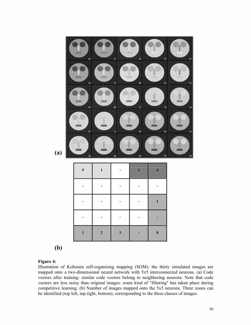
50

9

1

-

1

4

-

-

-

-

-

-

-

-

-

1

-

-

-

-

-

1

2

3

-

8

Figure 4: Illustration of Kohonen self-organizing mapping (SOM): the thirty simulated images are mapped onto a two-dimensional neural network with 5x5 interconnected neurons. (a) Code vectors after training: similar code vectors belong to neighboring neurons. Note that code vectors are less noisy than original images: some kind of "filtering" has taken place during competitive learning. (b) Number of images mapped onto the 5x5 neurons. Three zones can be identified (top left, top right, bottom), corresponding to the three classes of images.

(a)

(b)

51

Figure 5: Schematic representation of an auto-associative neural network (AANN). The first half of the network code the information in a set of D-dimensional input vectors (here D=4) into a D’-dimensional reduced space (here D’=2) in such a way that, after decoding by the second half of the network, the output vectors are as similar as possible to the input vectors. When training is performed, any D-dimensional vector of the set can be represented by a vector in a reduced (D’-dimensional) space.

Inpu

t

Input layer

Coding layer

Bottlenecklayer

Decodinglayer

Outputlayer

Out

put

52

Figure 6: Illustration of some tests for evaluating the quality of a mapping procedure. (a) The scatterplot test: distances between pairs of objects in the reduced space (dij) are

plotted against the distances between the same pairs of objects in the original space (Dij). A concentration of points along the first diagonal is an indication of a good mapping while a large dispersion of the points indicates that the mapping is poor and the dimension of the reduced space (D') is probably below the intrinsic dimension of the data set. This is illustrated here for Sammon's mapping of the 30 simulated images partly displayed in

(b

1 2 3 4

Dimension of the reduced space

Sam

mon

's c

riter

ion

(arb

itrar

y un

its)

D'=4 D'=3

D'=2 D'=1

(a

53

Figure 1. The intrinsic dimensionality in this case can be estimated to be equal to two, which is consistent with the fact that three sources of information are present (eyes, nose and mouth), but two of them (nose and mouth) are highly correlated (see Figure 2a).

(b) Plot of the Sammon criterion as a function of the dimension of the reduced space (D'). Although the distortion measure increases continuously when the dimension of the reduced space decreases, a shoulder in the curve may be an indication of the intrinsic dimensionality (here at D'=2), as expected.

Figure 7: Illustration of the use of three-dimensional scatterplots for Interactive Correlation Partitioning (ICP). From the three experimental images (a-c), a three-dimensional scatterplot is drawn and can be viewed from different points of view (e). Five main clouds of points (labeled 1 to 5) are depicted. Selecting one of them allows returning to the real space to visualize the localization of the corresponding pixels (not shown). Reproduced from Kenny et al. (1994) with permission of Elsevier Science B.V.

54

Figure 8: Schematic representation of a multi-layer feedforward neural network (MLFFNN). Here a three-layer network is represented, with four neurons in the input layer, three neurons in the (single) hidden layer and two neurons in the output layer.

Input layer

Hidden layer

Output layer

Inpu

t

Out

put

55

Figure9

3

Num

ber

of m

odes

Smoothing parameter

(a) (b)

(c) (d)

(e)

56

Figure 9: Illustration of automatic unsupervised classification of images with the Parzen/watersheds method. The method starts after the mapping of objects in a space of reduced (two or three) dimension: (a) Result of mapping the 30 simulated images (see Figure 1) onto a two- dimensional space. Here, the results of Correspondence Analysis are used (see Figure 2), but other nonlinear mapping methods can be used as well. (b) The second step consists in estimating the global probability density function by the Parzen method. Each mode of the pdf is assumed to define a class. Note that no assumption is made concerning the shape of the different classes. (c) The same result (rotated) is shown in three dimensions. The height of the peaks is an indication of the population in the different classes. (d) The parameter space is segmented (and labeled) into as many regions as there are modes in the pdf, according to the mathematical morphology watersheds method. The last step then involves giving the different objects the labels corresponding to their position in the parameter space. For this simple example with non-overlapping classes, the classification performance is 100%, but this is not the case when the distributions corresponding to the different classes overlap. (e) Curve showing the number of modes of the estimated probability density function versus the smoothing parameter characterizing the kernel used with the Parzen method. It is clear that, in this case, a large plateau is obtained for three classes. The smoothing parameter used for computing figure 9(b) was chosen at the middle of this plateau.

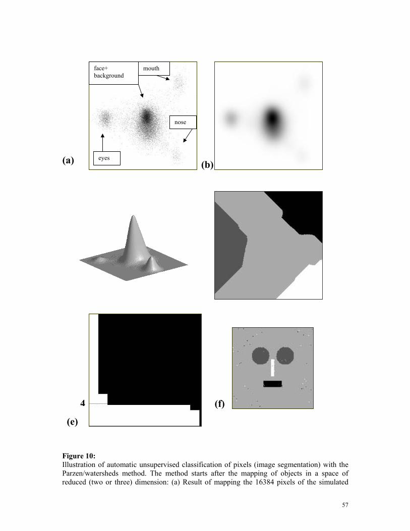
57

Figure 10: Illustration of automatic unsupervised classification of pixels (image segmentation) with the Parzen/watersheds method. The method starts after the mapping of objects in a space of reduced (two or three) dimension: (a) Result of mapping the 16384 pixels of the simulated

4 (f)

(b)

face+ background

eyes

mouth

nose

(a)

(e)

58

images (see figure 1) onto a two dimensional space. Here, the results of Correspondence Analysis are used (a scatterplot is drawn using the first two factorial images), but other nonlinear mapping methods can be used as well. (b) The second step consists in estimating the global probability density function, by the Parzen method. Each bump of the pdf is assumed to define a class. Note that no assumption is made concerning the shape of the different classes. (c) The same result (rotated) is shown in three dimensions. The height of the peaks is an indication of the population in the different classes. (d) The parameter space is segmented (and labeled) into as many regions as there are modes in the pdf, according to the mathematical morphology watersheds method. (e) Curve showing the number of modes of the estimated probability density function versus the smoothing parameter characterizing the kernel used with the Parzen method. One can see that, in this case, a large plateau is obtained for four classes. The smoothing parameter used for computing figure B was chosen at the middle of this plateau. (f) The last step then consists to gave the different objects (pixels) one of the four labels corresponding to their position in the parameter space. Figure 11: One of the first applications of automatic unsupervised classification to the segmentation of multi-component images in the field of microanalysis. (a) Series of µ-XRF elemental maps obtained out of the spectrum-image of a granite sample. (b) Score images (also called eigen-images) obtained by Principal Components Analysis of the images in 1. (c) Percentage of variance explained by the different principal components (top). Score plot (Principal components 1 and 2) showing the presence of three main classes of pixels (middle). Loading plot showing the correlation between the different chemical elements; see for instance the high positive correlation between Mn, Fe and Ti, and the anti-correlation between K and Ca (bottom). (d) Result of automatic classification into four classes using the C-means algorithm after PCA pre-treatment: individual and compound segmentation masks. Reproduced from Wekemans et al. (1997) with permission of John Wiley and Sons. Figure 12: One of the first examples of combination of dimensionality reduction (using Correspondence Analysis) and object classification in the reduced feature space -here the space spanned by the first two eigenvectors. Reproduced from Van Heel and Frank (1981) with permission of Elsevier Science B.V.. Figure 13: One of the first applications of Self-Organizing Maps (SOM) to the unsupervised classification of individual particle images. 1) Gallery of 25 out of the 407 particles used for the study. The images were translationally, but not rotationally aligned. 2) Code vectors associated with some of the 10x10 neurons of the map, after training. The particles with the same orientation are associated with the same neuron. 3) Enlargement of 2. 4) One of the images assigned to the neurons displayed in 3. Reproduced from Marabini and Carazo (1994) with permission of the Biophysical Journal Editorial Office.

59

(a)

(b)

Figure 14: Application of SOM to individual particles characterized by their rotational power spectrum. 1) The code vectors (rotational power spectra) associated with a Kohonen 7x7 map, after training with 2458 samples. Four regions can be distinguished, which differ by the order of the symmetry: region A (6-fold component + small 3-fold component); region B (2-fold component); region C (3-fold symmetry); region D (lack of predominant symmetry). 2) Rotational power spectra averages over regions A, D, B and C, respectively. Reproduced from Pascual et al. (1999) with permission of Springer-Verlag.

60

Figure 15: Illustration of automatic classification methods to the study of imperfect biological crystals. The crystal units were classified into four classes, which were subsequently averaged separately. Reproduced from Sherman et al. (1998) with permission of Elsevier Science B.V. Figure 16: The first application of supervised automatic classification techniques to crystalline subunits in material science. (a) High resolution transmission electron microscopy image of the (γ, γ')-interface in a Ni base superalloy. (b) Different results of the Maximum Likelihood classification procedure, for different values of tuning parameters. Reproduced from Aebersold et al. (1997) with permission of Elsevier Science B.V. Figure 17: Illustration of the use of the Hough transform for automatically analyzing convergent beam diffraction patterns. (a) Experimental <233> zone axis CBED pattern of aluminum. b) Corresponding Hough transform. The white lines in a) represent the line positions depicted as peaks in (b). Reproduced from Kramer and Mayer (1999) with permission of the Royal Microscopical Society, Oxford. Figure 18: Combined characterization of microparticles from shape analysis (fractal analysis) and Energy Dispersive X-ray spectroscopy. (A) Fly ash particle. (B) Soil dust particle. Reproduced from Kindratenko et al. (1996) with permission of Springer-Verlag.