Artificial Intelligence 06.01 introduction bayesian_networks
212
Artificial Intelligence Introduction to Bayesian Networks Andres Mendez-Vazquez March 2, 2016 1 / 85
-
Upload
andres-mendez-vazquez -
Category
Engineering
-
view
296 -
download
5
Transcript of Artificial Intelligence 06.01 introduction bayesian_networks
Artificial IntelligenceIntroduction to Bayesian Networks
Andres Mendez-Vazquez
March 2, 2016
1 / 85
Outline1 History
The History of Bayesian Applications
2 Bayes TheoremEverything Starts at SomeplaceWhy Bayesian Networks?
3 Bayesian NetworksDefinitionMarkov ConditionExample
Using the Markok ConditionRepresenting the Joint DistributionObservations
Causality and Bayesian NetworksPrecautionary Tale
Causal DAGInference in Bayesian NetworksExampleGeneral Strategy of InferenceInference - An Overview
2 / 85
Outline1 History
The History of Bayesian Applications
2 Bayes TheoremEverything Starts at SomeplaceWhy Bayesian Networks?
3 Bayesian NetworksDefinitionMarkov ConditionExample
Using the Markok ConditionRepresenting the Joint DistributionObservations
Causality and Bayesian NetworksPrecautionary Tale
Causal DAGInference in Bayesian NetworksExampleGeneral Strategy of InferenceInference - An Overview
3 / 85

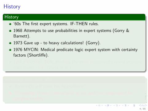
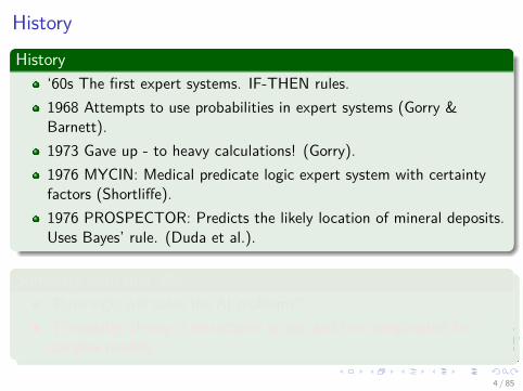
HistoryHistory
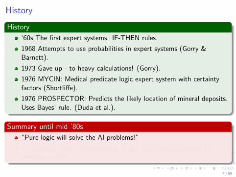
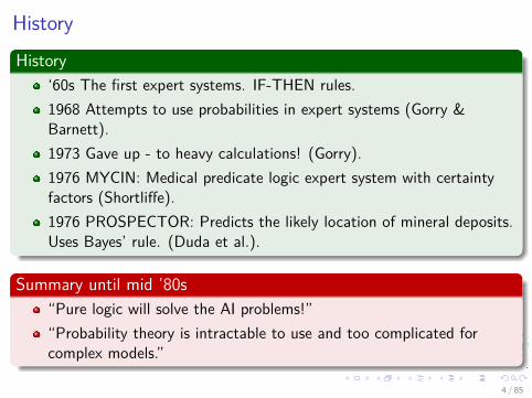
‘60s The first expert systems. IF-THEN rules.1968 Attempts to use probabilities in expert systems (Gorry &Barnett).1973 Gave up - to heavy calculations! (Gorry).1976 MYCIN: Medical predicate logic expert system with certaintyfactors (Shortliffe).1976 PROSPECTOR: Predicts the likely location of mineral deposits.Uses Bayes’ rule. (Duda et al.).
Summary until mid ’80s“Pure logic will solve the AI problems!”“Probability theory is intractable to use and too complicated forcomplex models.”
4 / 85

HistoryHistory
‘60s The first expert systems. IF-THEN rules.1968 Attempts to use probabilities in expert systems (Gorry &Barnett).1973 Gave up - to heavy calculations! (Gorry).1976 MYCIN: Medical predicate logic expert system with certaintyfactors (Shortliffe).1976 PROSPECTOR: Predicts the likely location of mineral deposits.Uses Bayes’ rule. (Duda et al.).
Summary until mid ’80s“Pure logic will solve the AI problems!”“Probability theory is intractable to use and too complicated forcomplex models.”
4 / 85
But...
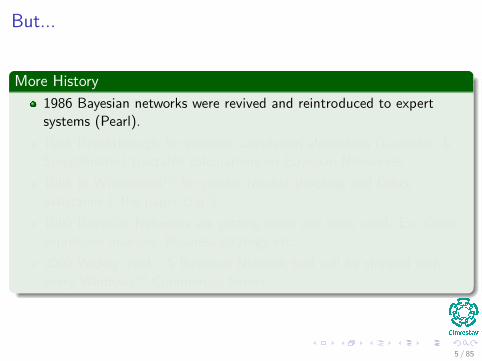
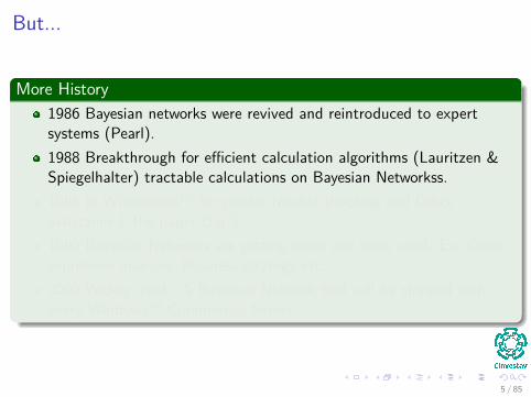
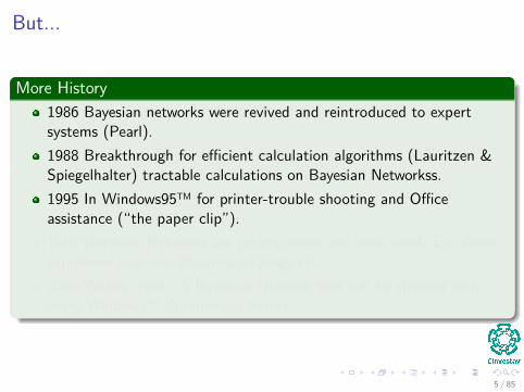
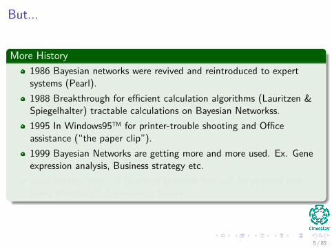
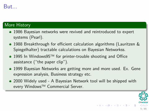
More History1986 Bayesian networks were revived and reintroduced to expertsystems (Pearl).1988 Breakthrough for efficient calculation algorithms (Lauritzen &Spiegelhalter) tractable calculations on Bayesian Networkss.1995 In Windows95™ for printer-trouble shooting and Officeassistance (“the paper clip”).1999 Bayesian Networks are getting more and more used. Ex. Geneexpression analysis, Business strategy etc.2000 Widely used - A Bayesian Network tool will be shipped withevery Windows™ Commercial Server.
5 / 85
But...
More History1986 Bayesian networks were revived and reintroduced to expertsystems (Pearl).1988 Breakthrough for efficient calculation algorithms (Lauritzen &Spiegelhalter) tractable calculations on Bayesian Networkss.1995 In Windows95™ for printer-trouble shooting and Officeassistance (“the paper clip”).1999 Bayesian Networks are getting more and more used. Ex. Geneexpression analysis, Business strategy etc.2000 Widely used - A Bayesian Network tool will be shipped withevery Windows™ Commercial Server.
5 / 85
Furtheron 2000-2015
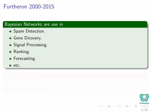
Bayesian Networks are use inSpam Detection.Gene Dicovery.Signal Processing.Ranking.Forecasting.etc.
Something NotableWe are interested more and more on building automatically BayesianNetworks using data!!!
6 / 85
Furtheron 2000-2015
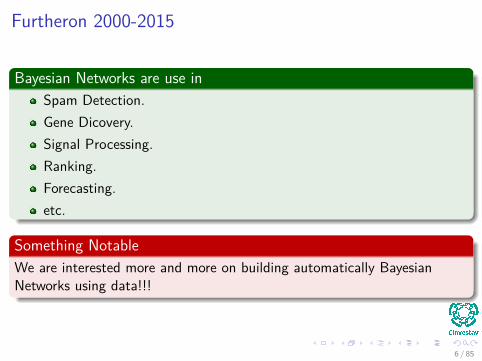
Bayesian Networks are use inSpam Detection.Gene Dicovery.Signal Processing.Ranking.Forecasting.etc.
Something NotableWe are interested more and more on building automatically BayesianNetworks using data!!!
6 / 85
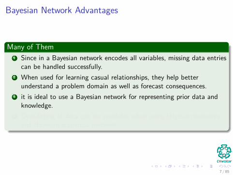
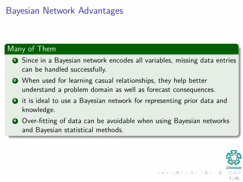
Bayesian Network Advantages
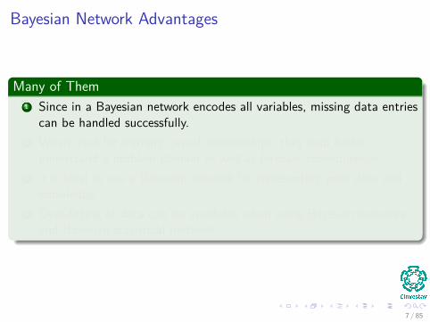
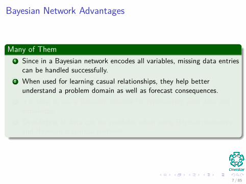
Many of Them1 Since in a Bayesian network encodes all variables, missing data entries
can be handled successfully.2 When used for learning casual relationships, they help better
understand a problem domain as well as forecast consequences.3 it is ideal to use a Bayesian network for representing prior data and
knowledge.4 Over-fitting of data can be avoidable when using Bayesian networks
and Bayesian statistical methods.
7 / 85
Bayesian Network Advantages
Many of Them1 Since in a Bayesian network encodes all variables, missing data entries
can be handled successfully.2 When used for learning casual relationships, they help better
understand a problem domain as well as forecast consequences.3 it is ideal to use a Bayesian network for representing prior data and
knowledge.4 Over-fitting of data can be avoidable when using Bayesian networks
and Bayesian statistical methods.
7 / 85
Outline1 History
The History of Bayesian Applications
2 Bayes TheoremEverything Starts at SomeplaceWhy Bayesian Networks?
3 Bayesian NetworksDefinitionMarkov ConditionExample
Using the Markok ConditionRepresenting the Joint DistributionObservations
Causality and Bayesian NetworksPrecautionary Tale
Causal DAGInference in Bayesian NetworksExampleGeneral Strategy of InferenceInference - An Overview
8 / 85
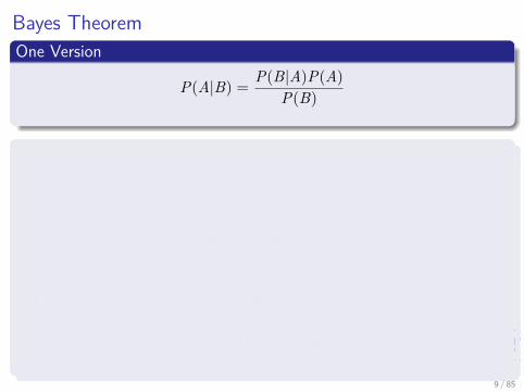
Bayes TheoremOne Version
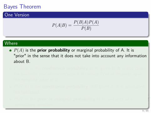
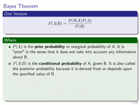
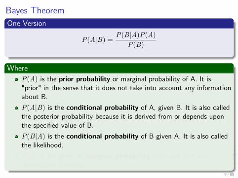
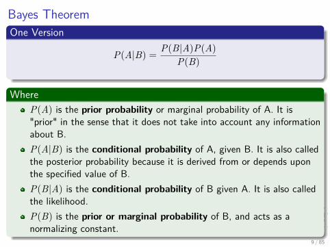
P(A|B) = P(B|A)P(A)P(B)
WhereP(A) is the prior probability or marginal probability of A. It is"prior" in the sense that it does not take into account any informationabout B.P(A|B) is the conditional probability of A, given B. It is also calledthe posterior probability because it is derived from or depends uponthe specified value of B.P(B|A) is the conditional probability of B given A. It is also calledthe likelihood.P(B) is the prior or marginal probability of B, and acts as anormalizing constant.
9 / 85
Bayes TheoremOne Version
P(A|B) = P(B|A)P(A)P(B)
WhereP(A) is the prior probability or marginal probability of A. It is"prior" in the sense that it does not take into account any informationabout B.P(A|B) is the conditional probability of A, given B. It is also calledthe posterior probability because it is derived from or depends uponthe specified value of B.P(B|A) is the conditional probability of B given A. It is also calledthe likelihood.P(B) is the prior or marginal probability of B, and acts as anormalizing constant.
9 / 85
A Simple Example
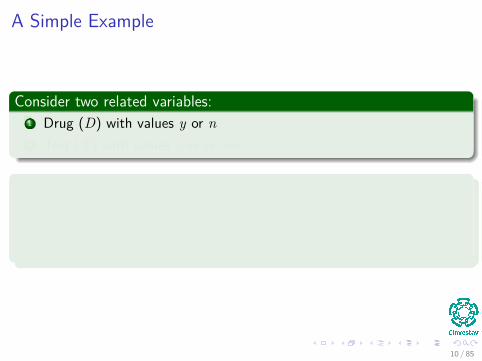
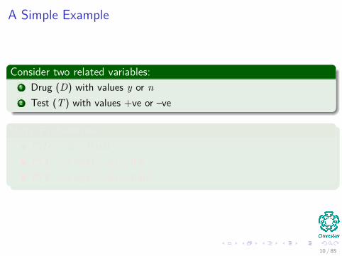
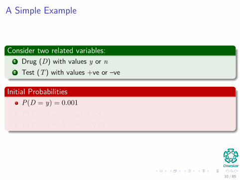
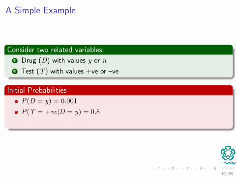
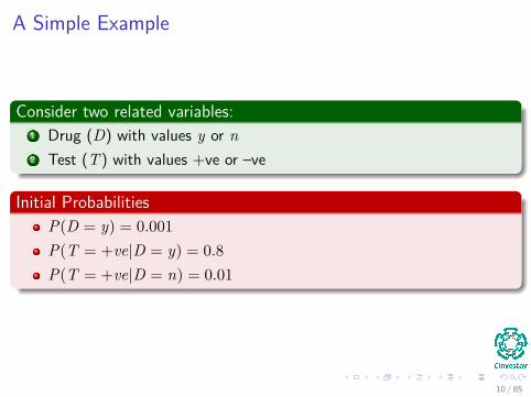
Consider two related variables:1 Drug (D) with values y or n2 Test (T ) with values +ve or –ve
Initial ProbabilitiesP(D = y) = 0.001P(T = +ve|D = y) = 0.8P(T = +ve|D = n) = 0.01
10 / 85
A Simple Example
Consider two related variables:1 Drug (D) with values y or n2 Test (T ) with values +ve or –ve
Initial ProbabilitiesP(D = y) = 0.001P(T = +ve|D = y) = 0.8P(T = +ve|D = n) = 0.01
10 / 85
A Simple Example
Consider two related variables:1 Drug (D) with values y or n2 Test (T ) with values +ve or –ve
Initial ProbabilitiesP(D = y) = 0.001P(T = +ve|D = y) = 0.8P(T = +ve|D = n) = 0.01
10 / 85
A Simple Example
Consider two related variables:1 Drug (D) with values y or n2 Test (T ) with values +ve or –ve
Initial ProbabilitiesP(D = y) = 0.001P(T = +ve|D = y) = 0.8P(T = +ve|D = n) = 0.01
10 / 85
A Simple Example
Consider two related variables:1 Drug (D) with values y or n2 Test (T ) with values +ve or –ve
Initial ProbabilitiesP(D = y) = 0.001P(T = +ve|D = y) = 0.8P(T = +ve|D = n) = 0.01
10 / 85
A Simple Example
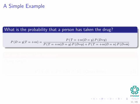
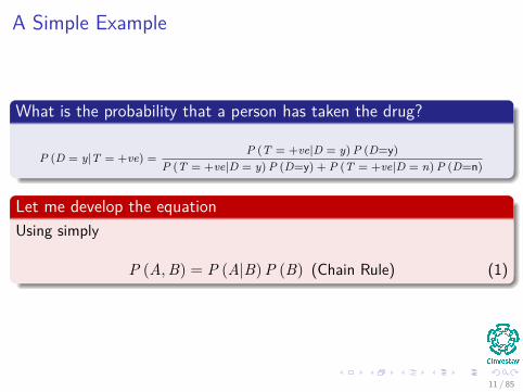
What is the probability that a person has taken the drug?
P (D = y|T = +ve) =P (T = +ve|D = y) P (D=y)
P (T = +ve|D = y) P (D=y) + P (T = +ve|D = n) P (D=n)
Let me develop the equationUsing simply
P (A, B) = P (A|B) P (B) (Chain Rule) (1)
11 / 85
A Simple Example
What is the probability that a person has taken the drug?
P (D = y|T = +ve) =P (T = +ve|D = y) P (D=y)
P (T = +ve|D = y) P (D=y) + P (T = +ve|D = n) P (D=n)
Let me develop the equationUsing simply
P (A, B) = P (A|B) P (B) (Chain Rule) (1)
11 / 85
Outline1 History
The History of Bayesian Applications
2 Bayes TheoremEverything Starts at SomeplaceWhy Bayesian Networks?
3 Bayesian NetworksDefinitionMarkov ConditionExample
Using the Markok ConditionRepresenting the Joint DistributionObservations
Causality and Bayesian NetworksPrecautionary Tale
Causal DAGInference in Bayesian NetworksExampleGeneral Strategy of InferenceInference - An Overview
12 / 85
A More Complex Case
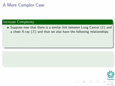
Increase ComplexitySuppose now that there is a similar link between Lung Cancer (L) anda chest X-ray (X) and that we also have the following relationships:
I History of smoking (S) has a direct influence on bronchitis (B) andlung cancer (L);
I L and B have a direct influence on fatigue (F).
QuestionWhat is the probability that someone has bronchitis given that theysmoke, have fatigue and have received a positive X-ray result?
13 / 85
A More Complex Case
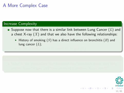
Increase ComplexitySuppose now that there is a similar link between Lung Cancer (L) anda chest X-ray (X) and that we also have the following relationships:
I History of smoking (S) has a direct influence on bronchitis (B) andlung cancer (L);
I L and B have a direct influence on fatigue (F).
QuestionWhat is the probability that someone has bronchitis given that theysmoke, have fatigue and have received a positive X-ray result?
13 / 85
A More Complex Case
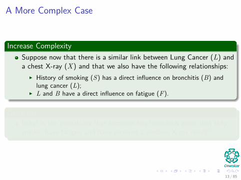
Increase ComplexitySuppose now that there is a similar link between Lung Cancer (L) anda chest X-ray (X) and that we also have the following relationships:
I History of smoking (S) has a direct influence on bronchitis (B) andlung cancer (L);
I L and B have a direct influence on fatigue (F).
QuestionWhat is the probability that someone has bronchitis given that theysmoke, have fatigue and have received a positive X-ray result?
13 / 85

A More Complex Case
Increase ComplexitySuppose now that there is a similar link between Lung Cancer (L) anda chest X-ray (X) and that we also have the following relationships:
I History of smoking (S) has a direct influence on bronchitis (B) andlung cancer (L);
I L and B have a direct influence on fatigue (F).
QuestionWhat is the probability that someone has bronchitis given that theysmoke, have fatigue and have received a positive X-ray result?
13 / 85
A More Complex Case
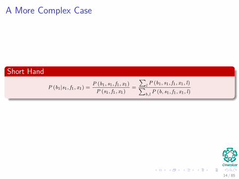
Short Hand
P (b1|s1, f1, x1) =P (b1, s1, f1, x1)
P (s1, f1, x1)=
∑l P (b1, s1, f1, x1, l)∑b,l P (b, s1, f1, x1, l)
14 / 85
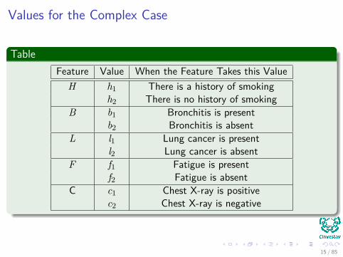
Values for the Complex Case
TableFeature Value When the Feature Takes this Value
H h1 There is a history of smokingh2 There is no history of smoking
B b1 Bronchitis is presentb2 Bronchitis is absent
L l1 Lung cancer is presentl2 Lung cancer is absent
F f1 Fatigue is presentf2 Fatigue is absent
C c1 Chest X-ray is positivec2 Chest X-ray is negative
15 / 85
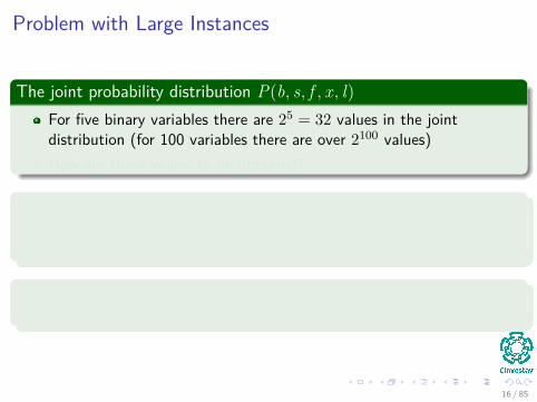
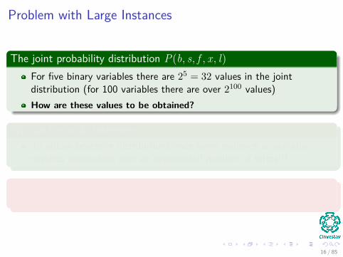
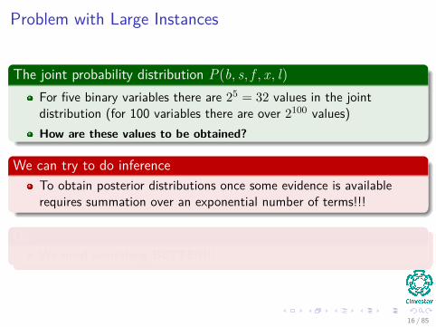
Problem with Large Instances
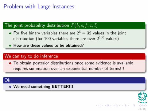
The joint probability distribution P(b, s, f , x , l)For five binary variables there are 25 = 32 values in the jointdistribution (for 100 variables there are over 2100 values)How are these values to be obtained?
We can try to do inferenceTo obtain posterior distributions once some evidence is availablerequires summation over an exponential number of terms!!!
OkWe need something BETTER!!!
16 / 85
Problem with Large Instances
The joint probability distribution P(b, s, f , x , l)For five binary variables there are 25 = 32 values in the jointdistribution (for 100 variables there are over 2100 values)How are these values to be obtained?
We can try to do inferenceTo obtain posterior distributions once some evidence is availablerequires summation over an exponential number of terms!!!
OkWe need something BETTER!!!
16 / 85
Outline1 History
The History of Bayesian Applications
2 Bayes TheoremEverything Starts at SomeplaceWhy Bayesian Networks?
3 Bayesian NetworksDefinitionMarkov ConditionExample
Using the Markok ConditionRepresenting the Joint DistributionObservations
Causality and Bayesian NetworksPrecautionary Tale
Causal DAGInference in Bayesian NetworksExampleGeneral Strategy of InferenceInference - An Overview
17 / 85
Bayesian Networks
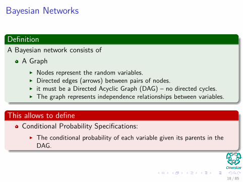
DefinitionA Bayesian network consists of
A GraphI Nodes represent the random variables.I Directed edges (arrows) between pairs of nodes.I it must be a Directed Acyclic Graph (DAG) – no directed cycles.I The graph represents independence relationships between variables.
This allows to defineConditional Probability Specifications:
I The conditional probability of each variable given its parents in theDAG.
18 / 85
Bayesian Networks
DefinitionA Bayesian network consists of
A GraphI Nodes represent the random variables.I Directed edges (arrows) between pairs of nodes.I it must be a Directed Acyclic Graph (DAG) – no directed cycles.I The graph represents independence relationships between variables.
This allows to defineConditional Probability Specifications:
I The conditional probability of each variable given its parents in theDAG.
18 / 85
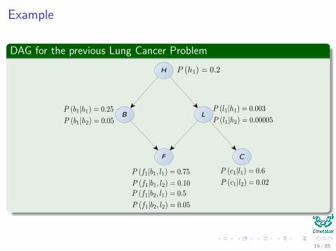
Example
DAG for the previous Lung Cancer ProblemH
B L
F C
19 / 85
Outline1 History
The History of Bayesian Applications
2 Bayes TheoremEverything Starts at SomeplaceWhy Bayesian Networks?
3 Bayesian NetworksDefinitionMarkov ConditionExample
Using the Markok ConditionRepresenting the Joint DistributionObservations
Causality and Bayesian NetworksPrecautionary Tale
Causal DAGInference in Bayesian NetworksExampleGeneral Strategy of InferenceInference - An Overview
20 / 85
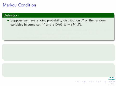
Markov Condition
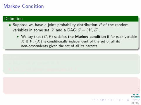
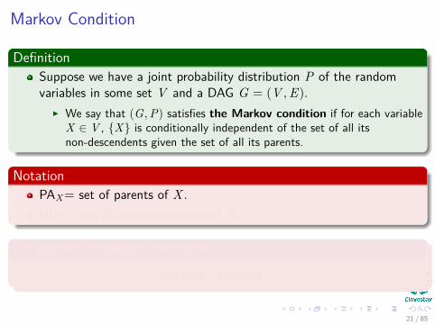
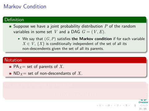
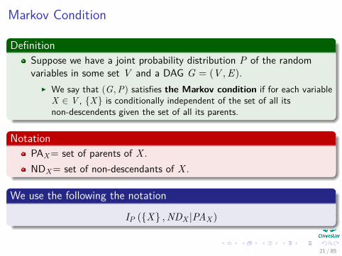
DefinitionSuppose we have a joint probability distribution P of the randomvariables in some set V and a DAG G = (V , E).
I We say that (G, P) satisfies the Markov condition if for each variableX ∈ V , {X} is conditionally independent of the set of all itsnon-descendents given the set of all its parents.
NotationPAX= set of parents of X .NDX= set of non-descendants of X .
We use the following the notation
IP ({X} , NDX |PAX )
21 / 85
Markov Condition
DefinitionSuppose we have a joint probability distribution P of the randomvariables in some set V and a DAG G = (V , E).
I We say that (G, P) satisfies the Markov condition if for each variableX ∈ V , {X} is conditionally independent of the set of all itsnon-descendents given the set of all its parents.
NotationPAX= set of parents of X .NDX= set of non-descendants of X .
We use the following the notation
IP ({X} , NDX |PAX )
21 / 85
Outline1 History
The History of Bayesian Applications
2 Bayes TheoremEverything Starts at SomeplaceWhy Bayesian Networks?
3 Bayesian NetworksDefinitionMarkov ConditionExample
Using the Markok ConditionRepresenting the Joint DistributionObservations
Causality and Bayesian NetworksPrecautionary Tale
Causal DAGInference in Bayesian NetworksExampleGeneral Strategy of InferenceInference - An Overview
22 / 85
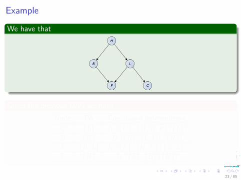
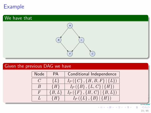
Example
We have thatH
B L
F C
Given the previous DAG we haveNode PA Conditional Independence
C {L} IP ({C} , {H , B, F} | {L})B {H} IP ({B} , {L, C} | {H})F {B, L} IP ({F} , {H , C} | {B, L})L {H} IP ({L} , {B} | {H})
23 / 85
Example
We have thatH
B L
F C
Given the previous DAG we haveNode PA Conditional Independence
C {L} IP ({C} , {H , B, F} | {L})B {H} IP ({B} , {L, C} | {H})F {B, L} IP ({F} , {H , C} | {B, L})L {H} IP ({L} , {B} | {H})
23 / 85
Outline1 History
The History of Bayesian Applications
2 Bayes TheoremEverything Starts at SomeplaceWhy Bayesian Networks?
3 Bayesian NetworksDefinitionMarkov ConditionExample
Using the Markok ConditionRepresenting the Joint DistributionObservations
Causality and Bayesian NetworksPrecautionary Tale
Causal DAGInference in Bayesian NetworksExampleGeneral Strategy of InferenceInference - An Overview
24 / 85
Using the Markov Condition
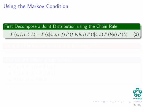
First Decompose a Joint Distribution using the Chain RuleP (c, f , l, b, h) = P (c|b, s, l, f ) P (f |b, h, l) P (l|b, h) P (b|h) P (h) (2)
Using the Markov condition in the following DAG
We have the following equivalencesP (c|b, h, l, f ) = P (c|l)P (f |b, h, l) = P (f |b, l)P (l|b, h) = P (l|h)
25 / 85
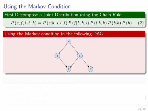
Using the Markov ConditionFirst Decompose a Joint Distribution using the Chain Rule
P (c, f , l, b, h) = P (c|b, s, l, f ) P (f |b, h, l) P (l|b, h) P (b|h) P (h) (2)
Using the Markov condition in the following DAGH
B L
F C
We have the following equivalencesP (c|b, h, l, f ) = P (c|l)P (f |b, h, l) = P (f |b, l)P (l|b, h) = P (l|h)
25 / 85
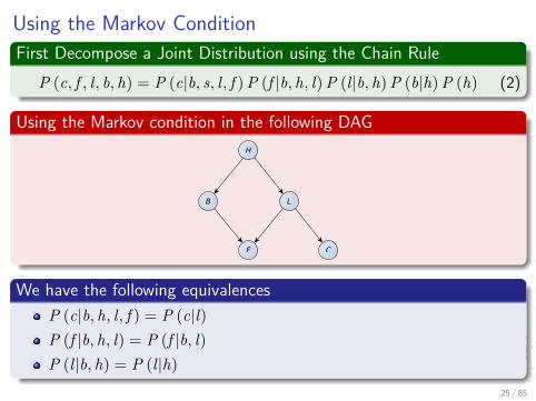
Using the Markov ConditionFirst Decompose a Joint Distribution using the Chain Rule
P (c, f , l, b, h) = P (c|b, s, l, f ) P (f |b, h, l) P (l|b, h) P (b|h) P (h) (2)
Using the Markov condition in the following DAGH
B L
F C
We have the following equivalencesP (c|b, h, l, f ) = P (c|l)P (f |b, h, l) = P (f |b, l)P (l|b, h) = P (l|h)
25 / 85
Using the Markov Condition
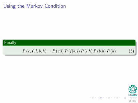
Finally
P (c, f , l, b, h) = P (c|l) P (f |b, l) P (l|h) P (b|h) P (h) (3)
26 / 85
Outline1 History
The History of Bayesian Applications
2 Bayes TheoremEverything Starts at SomeplaceWhy Bayesian Networks?
3 Bayesian NetworksDefinitionMarkov ConditionExample
Using the Markok ConditionRepresenting the Joint DistributionObservations
Causality and Bayesian NetworksPrecautionary Tale
Causal DAGInference in Bayesian NetworksExampleGeneral Strategy of InferenceInference - An Overview
27 / 85
Representing the Joint Distribution
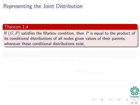
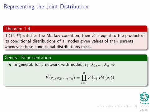
Theorem 1.4If (G, P) satisfies the Markov condition, then P is equal to the product ofits conditional distributions of all nodes given values of their parents,whenever these conditional distributions exist.
General RepresentationIn general, for a network with nodes X1, X2, ..., Xn ⇒
P (x1, x2, ..., xn) =n∏
i=1P (xi |PA (xi))
28 / 85
Representing the Joint Distribution
Theorem 1.4If (G, P) satisfies the Markov condition, then P is equal to the product ofits conditional distributions of all nodes given values of their parents,whenever these conditional distributions exist.
General RepresentationIn general, for a network with nodes X1, X2, ..., Xn ⇒
P (x1, x2, ..., xn) =n∏
i=1P (xi |PA (xi))
28 / 85
Proof of Theorem 1.4
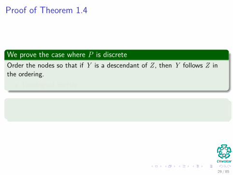
We prove the case where P is discreteOrder the nodes so that if Y is a descendant of Z , then Y follows Z inthe ordering.
Topological Sorting.
This is calledAncestral ordering.
29 / 85
Proof of Theorem 1.4
We prove the case where P is discreteOrder the nodes so that if Y is a descendant of Z , then Y follows Z inthe ordering.
Topological Sorting.
This is calledAncestral ordering.
29 / 85
Proof of Theorem 1.4
We prove the case where P is discreteOrder the nodes so that if Y is a descendant of Z , then Y follows Z inthe ordering.
Topological Sorting.
This is calledAncestral ordering.
29 / 85
Proof
For example
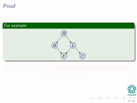
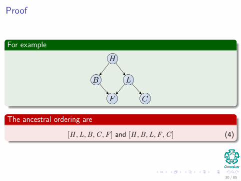
The ancestral ordering are
[H , L, B, C , F ] and [H , B, L, F , C ] (4)
30 / 85
Proof
For example
The ancestral ordering are
[H , L, B, C , F ] and [H , B, L, F , C ] (4)
30 / 85

Proof
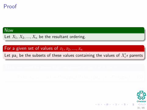
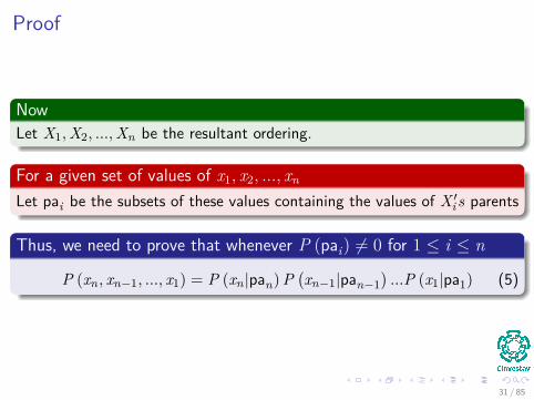
NowLet X1, X2, ..., Xn be the resultant ordering.
For a given set of values of x1, x2, ..., xn
Let pai be the subsets of these values containing the values of X ′i s parents
Thus, we need to prove that whenever P (pai) 6= 0 for 1 ≤ i ≤ n
P (xn , xn−1, ..., x1) = P (xn |pan) P(xn−1|pan−1
)...P (x1|pa1) (5)
31 / 85
Proof
NowLet X1, X2, ..., Xn be the resultant ordering.
For a given set of values of x1, x2, ..., xn
Let pai be the subsets of these values containing the values of X ′i s parents
Thus, we need to prove that whenever P (pai) 6= 0 for 1 ≤ i ≤ n
P (xn , xn−1, ..., x1) = P (xn |pan) P(xn−1|pan−1
)...P (x1|pa1) (5)
31 / 85
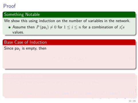
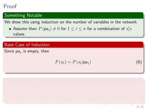
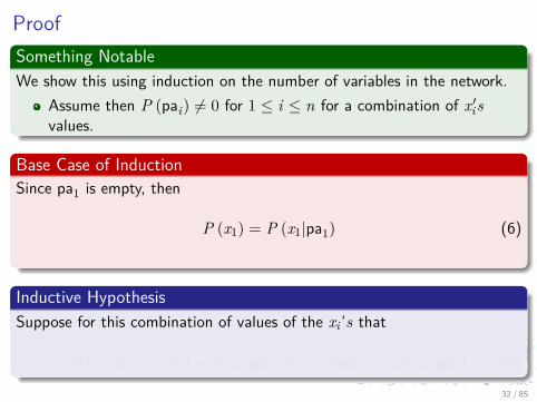
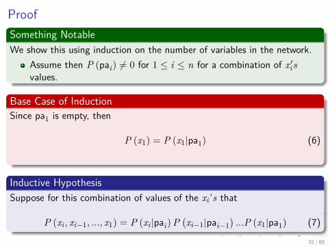
ProofSomething NotableWe show this using induction on the number of variables in the network.
Assume then P (pai) 6= 0 for 1 ≤ i ≤ n for a combination of x ′isvalues.
Base Case of InductionSince pa1 is empty, then
P (x1) = P (x1|pa1) (6)
Inductive HypothesisSuppose for this combination of values of the xi ’s that
P (xi , xi−1, ..., x1) = P (xi |pai) P(xi−1|pai−1
)...P (x1|pa1) (7)
32 / 85
Proof
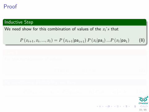
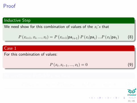
Inductive StepWe need show for this combination of values of the xi ’s that
P (xi+1, xi , ..., x1) = P(xi+1|pai+1
)P (xi |pai) ...P (x1|pa1) (8)
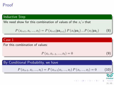
Case 1For this combination of values:
P (xi , xi−1, ..., x1) = 0 (9)
By Conditional Probability, we have
P (xi+1, xi , ..., x1) = P (xi+1|xi , ..., x1) P (xi , ..., x1) = 0 (10)
33 / 85
Proof
Inductive StepWe need show for this combination of values of the xi ’s that
P (xi+1, xi , ..., x1) = P(xi+1|pai+1
)P (xi |pai) ...P (x1|pa1) (8)
Case 1For this combination of values:
P (xi , xi−1, ..., x1) = 0 (9)
By Conditional Probability, we have
P (xi+1, xi , ..., x1) = P (xi+1|xi , ..., x1) P (xi , ..., x1) = 0 (10)
33 / 85
Proof
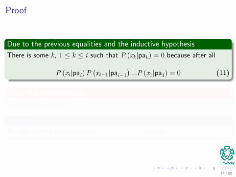
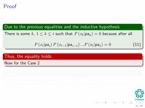
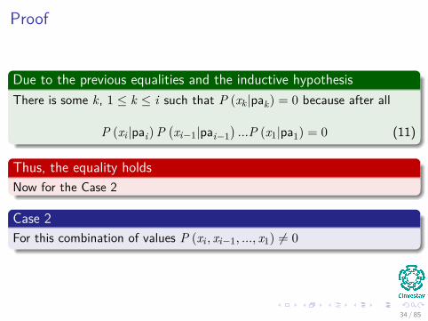
Due to the previous equalities and the inductive hypothesisThere is some k, 1 ≤ k ≤ i such that P (xk |pak) = 0 because after all
P (xi |pai) P(xi−1|pai−1
)...P (x1|pa1) = 0 (11)
Thus, the equality holdsNow for the Case 2
Case 2For this combination of values P (xi , xi−1, ..., x1) 6= 0
34 / 85
Proof
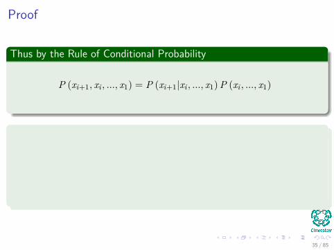
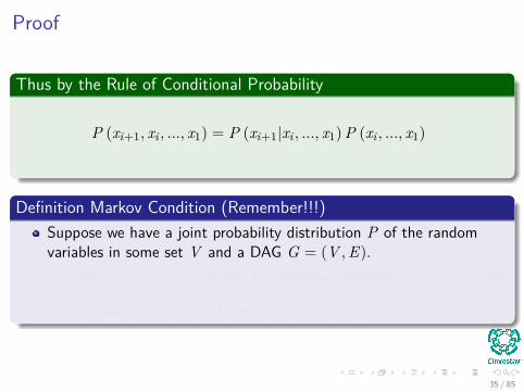
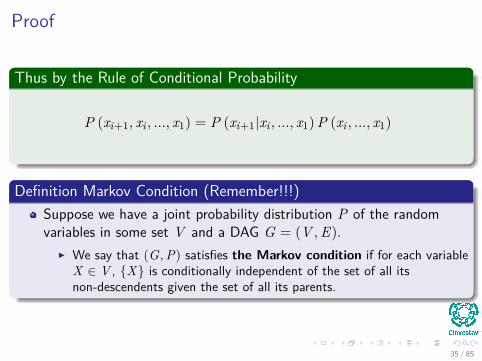
Thus by the Rule of Conditional Probability
P (xi+1, xi , ..., x1) = P (xi+1|xi , ..., x1) P (xi , ..., x1)
Definition Markov Condition (Remember!!!)Suppose we have a joint probability distribution P of the randomvariables in some set V and a DAG G = (V , E).
I We say that (G, P) satisfies the Markov condition if for each variableX ∈ V , {X} is conditionally independent of the set of all itsnon-descendents given the set of all its parents.
35 / 85
Proof
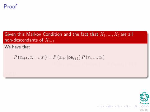
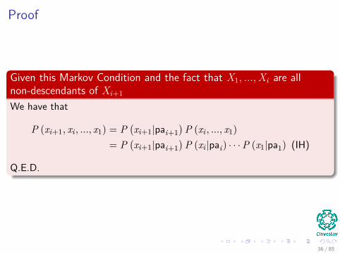
Given this Markov Condition and the fact that X1, ..., Xi are allnon-descendants of Xi+1
We have that
P (xi+1, xi , ..., x1) = P(xi+1|pai+1
)P (xi , ..., x1)
= P(xi+1|pai+1
)P (xi |pai) · · ·P (x1|pa1) (IH)
Q.E.D.
36 / 85
Proof
Given this Markov Condition and the fact that X1, ..., Xi are allnon-descendants of Xi+1
We have that
P (xi+1, xi , ..., x1) = P(xi+1|pai+1
)P (xi , ..., x1)
= P(xi+1|pai+1
)P (xi |pai) · · ·P (x1|pa1) (IH)
Q.E.D.
36 / 85
Outline1 History
The History of Bayesian Applications
2 Bayes TheoremEverything Starts at SomeplaceWhy Bayesian Networks?
3 Bayesian NetworksDefinitionMarkov ConditionExample
Using the Markok ConditionRepresenting the Joint DistributionObservations
Causality and Bayesian NetworksPrecautionary Tale
Causal DAGInference in Bayesian NetworksExampleGeneral Strategy of InferenceInference - An Overview
37 / 85

Now
OBSERVATIONS1 An enormous saving can be made regarding the number of values
required for the joint distribution.2 To determine the joint distribution directly for n binary variables 2n
values are required.3 For a Bayesian Network with n binary variables and each node has at
most k parents then less than 2kn values are required!!!
38 / 85
It is more!!!
Theorem 1.5Let a DAG G be given in which each node is a random variable, andlet a discrete conditional probability distribution of each node givenvalues of its parents in G be specified.Then, the product of these conditional distributions yields a jointprobability distribution P of the variables, and (G, P) satisfies theMarkov condition.
NoteNotice that the theorem requires that specified conditionaldistributions be discrete.Often in the case of continuous distributions it still holds.
39 / 85
Outline1 History
The History of Bayesian Applications
2 Bayes TheoremEverything Starts at SomeplaceWhy Bayesian Networks?
3 Bayesian NetworksDefinitionMarkov ConditionExample
Using the Markok ConditionRepresenting the Joint DistributionObservations
Causality and Bayesian NetworksPrecautionary Tale
Causal DAGInference in Bayesian NetworksExampleGeneral Strategy of InferenceInference - An Overview
40 / 85
Causality in Bayesian Networks
Definition of a CauseThe one, such as a person, an event, or a condition, that is responsible foran action or a result.
HoweverAlthough useful, this simple definition is certainly not the last word on theconcept of causation.
Actually Philosophers are still wrangling the issue!!!
41 / 85
Causality in Bayesian Networks
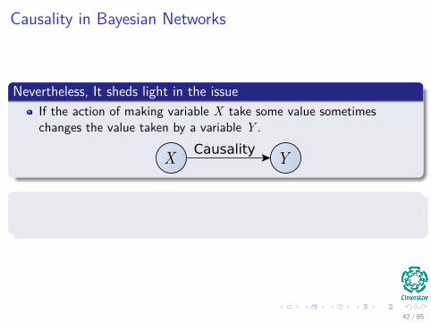
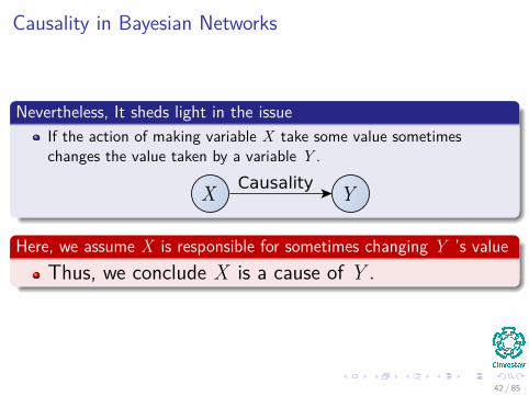
Nevertheless, It sheds light in the issueIf the action of making variable X take some value sometimeschanges the value taken by a variable Y .
Causality
Here, we assume X is responsible for sometimes changing Y ’s valueThus, we conclude X is a cause of Y .
42 / 85
Causality in Bayesian Networks
Nevertheless, It sheds light in the issueIf the action of making variable X take some value sometimeschanges the value taken by a variable Y .
Causality
Here, we assume X is responsible for sometimes changing Y ’s valueThus, we conclude X is a cause of Y .
42 / 85
Furthermore
FormallyWe say we manipulate X when we force X to take some value.
We say X causes Y if there is some manipulation of X that leads toa change in the probability distribution of Y .
ThusWe assume causes and their effects are statistically correlated.
HoweverVariables can be correlated without one causing the other.
43 / 85

Outline1 History
The History of Bayesian Applications
2 Bayes TheoremEverything Starts at SomeplaceWhy Bayesian Networks?
3 Bayesian NetworksDefinitionMarkov ConditionExample
Using the Markok ConditionRepresenting the Joint DistributionObservations
Causality and Bayesian NetworksPrecautionary Tale
Causal DAGInference in Bayesian NetworksExampleGeneral Strategy of InferenceInference - An Overview
44 / 85
Precautionary Tale: Causality and Bayesian Networks
ImportantNot every Bayesian Networks describes causal relationships between thevariables.
ConsiderConsider the dependence between Lung Cancer, L, and the X-raytest, X .By focusing on just these variables we might be tempted to representthem by the following Bayesian Networks.
45 / 85
Precautionary Tale: Causality and Bayesian Networks
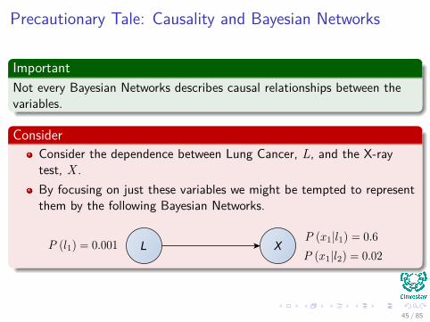
ImportantNot every Bayesian Networks describes causal relationships between thevariables.
ConsiderConsider the dependence between Lung Cancer, L, and the X-raytest, X .By focusing on just these variables we might be tempted to representthem by the following Bayesian Networks.
L X
45 / 85
Precautionary Tale: Causality and Bayesian Networks
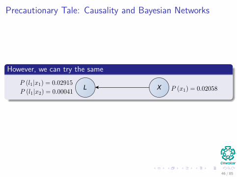
However, we can try the same
L X
46 / 85
Remark
Be CarefulIt is tempting to think that Bayesian Networkss can be created by creatinga DAG where the edges represent direct causal relationships between thevariables.
47 / 85
Outline1 History
The History of Bayesian Applications
2 Bayes TheoremEverything Starts at SomeplaceWhy Bayesian Networks?
3 Bayesian NetworksDefinitionMarkov ConditionExample
Using the Markok ConditionRepresenting the Joint DistributionObservations
Causality and Bayesian NetworksPrecautionary Tale
Causal DAGInference in Bayesian NetworksExampleGeneral Strategy of InferenceInference - An Overview
48 / 85
However
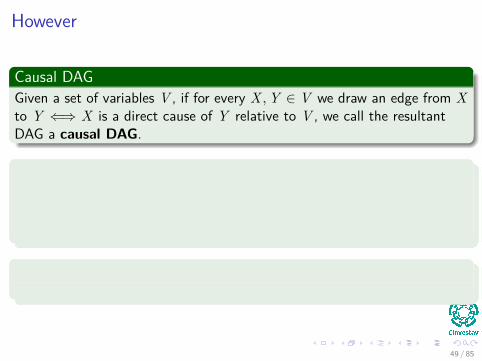
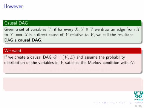
Causal DAGGiven a set of variables V , if for every X , Y ∈ V we draw an edge from Xto Y ⇐⇒ X is a direct cause of Y relative to V , we call the resultantDAG a causal DAG.
We wantIf we create a causal DAG G = (V , E) and assume the probabilitydistribution of the variables in V satisfies the Markov condition with G:
we say we are making the causal Markov assumption.
In GeneralThe Markov condition holds for a causal DAG.
49 / 85
However
Causal DAGGiven a set of variables V , if for every X , Y ∈ V we draw an edge from Xto Y ⇐⇒ X is a direct cause of Y relative to V , we call the resultantDAG a causal DAG.
We wantIf we create a causal DAG G = (V , E) and assume the probabilitydistribution of the variables in V satisfies the Markov condition with G:
we say we are making the causal Markov assumption.
In GeneralThe Markov condition holds for a causal DAG.
49 / 85

However, we still want to know if the Markov ConditionHolds
RemarkThere are several thing that the DAG needs to have in order to have theMarkov Condition.
Examples of thoseCommon CausesCommon Effects
50 / 85
However, we still want to know if the Markov ConditionHolds
RemarkThere are several thing that the DAG needs to have in order to have theMarkov Condition.
Examples of thoseCommon CausesCommon Effects
50 / 85
However, we still want to know if the Markov ConditionHolds
RemarkThere are several thing that the DAG needs to have in order to have theMarkov Condition.
Examples of thoseCommon CausesCommon Effects
50 / 85
How to have a Markov Assumption : Common Causes
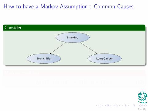
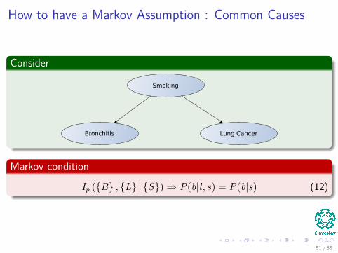
Consider
Smoking
Bronchitis Lung Cancer
Markov condition
Ip ({B} , {L} | {S})⇒ P(b|l, s) = P(b|s) (12)
51 / 85
How to have a Markov Assumption : Common Causes
Consider
Smoking
Bronchitis Lung Cancer
Markov condition
Ip ({B} , {L} | {S})⇒ P(b|l, s) = P(b|s) (12)
51 / 85
How to have a Markov Assumption : Common Causes
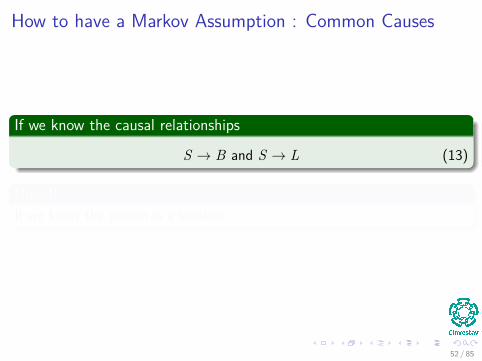
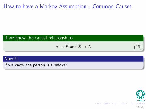
If we know the causal relationships
S → B and S → L (13)
Now!!!If we know the person is a smoker.
52 / 85
How to have a Markov Assumption : Common Causes
If we know the causal relationships
S → B and S → L (13)
Now!!!If we know the person is a smoker.
52 / 85
How to have a Markov Assumption : Common Causes
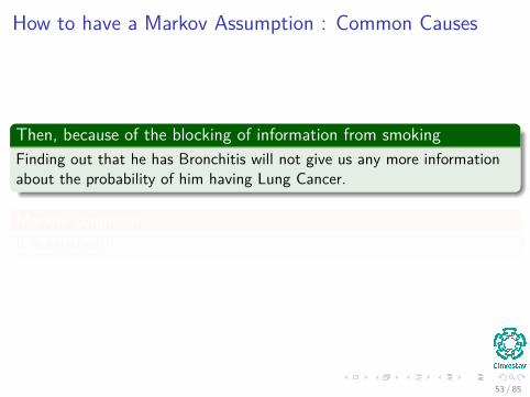
Then, because of the blocking of information from smokingFinding out that he has Bronchitis will not give us any more informationabout the probability of him having Lung Cancer.
Markov conditionIt is satisfied!!!
53 / 85
How to have a Markov Assumption : Common Causes
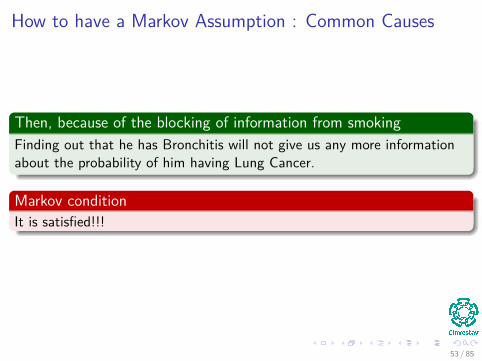
Then, because of the blocking of information from smokingFinding out that he has Bronchitis will not give us any more informationabout the probability of him having Lung Cancer.
Markov conditionIt is satisfied!!!
53 / 85
How to have a Markov Assumption : Common Effects
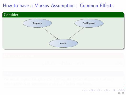
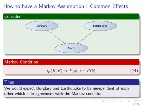
Consider
Alarm
Burglary Earthquake
Markov Condition
lp (B, E)⇒ P(b|e) = P(b) (14)
ThusWe would expect Burglary and Earthquake to be independent of eachother which is in agreement with the Markov condition.
54 / 85
How to have a Markov Assumption : Common Effects
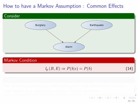
Consider
Alarm
Burglary Earthquake
Markov Condition
lp (B, E)⇒ P(b|e) = P(b) (14)
ThusWe would expect Burglary and Earthquake to be independent of eachother which is in agreement with the Markov condition.
54 / 85
How to have a Markov Assumption : Common Effects
Consider
Alarm
Burglary Earthquake
Markov Condition
lp (B, E)⇒ P(b|e) = P(b) (14)
ThusWe would expect Burglary and Earthquake to be independent of eachother which is in agreement with the Markov condition.
54 / 85
How to have a Markov Assumption : Common Effects
HoweverWe would, however expect them to be conditionally dependent givenAlarm.
ThusIf the alarm has gone off, news that there had been an earthquake would‘explain away’ the idea that a burglary had taken place.
ThenAgain in agreement with the Markov condition.
55 / 85

The Causal Markov Condition
What do we want?The basic idea is that the Markov condition holds for a causal DAG.
56 / 85
Rules to construct A Causal Graph
Conditions1 There must be no hidden common causes.2 There must not be selection bias.3 There must be no feedback loops.
ObservationsEven with these there is a lot of controversy as to its validity.It seems to be false in quantum mechanical.
57 / 85
Rules to construct A Causal Graph
Conditions1 There must be no hidden common causes.2 There must not be selection bias.3 There must be no feedback loops.
ObservationsEven with these there is a lot of controversy as to its validity.It seems to be false in quantum mechanical.
57 / 85
Rules to construct A Causal Graph
Conditions1 There must be no hidden common causes.2 There must not be selection bias.3 There must be no feedback loops.
ObservationsEven with these there is a lot of controversy as to its validity.It seems to be false in quantum mechanical.
57 / 85
Rules to construct A Causal Graph
Conditions1 There must be no hidden common causes.2 There must not be selection bias.3 There must be no feedback loops.
ObservationsEven with these there is a lot of controversy as to its validity.It seems to be false in quantum mechanical.
57 / 85
Rules to construct A Causal Graph
Conditions1 There must be no hidden common causes.2 There must not be selection bias.3 There must be no feedback loops.
ObservationsEven with these there is a lot of controversy as to its validity.It seems to be false in quantum mechanical.
57 / 85
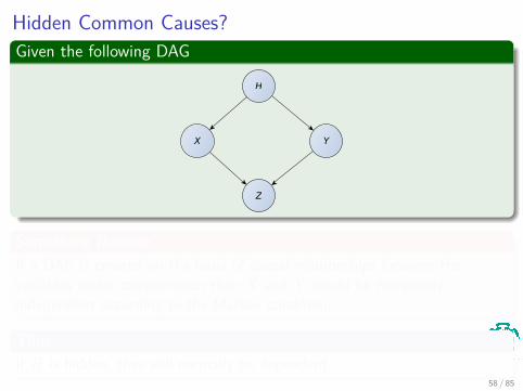
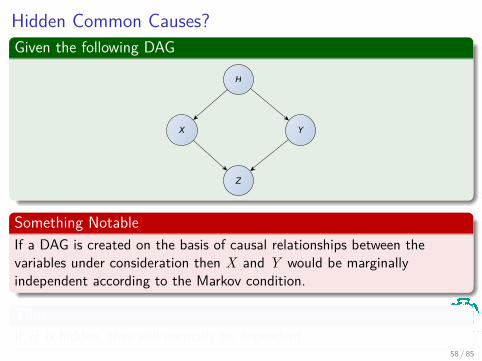
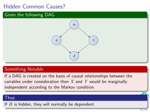
Hidden Common Causes?Given the following DAG
H
X Y
Z
Something NotableIf a DAG is created on the basis of causal relationships between thevariables under consideration then X and Y would be marginallyindependent according to the Markov condition.
ThusIf H is hidden, they will normally be dependent.
58 / 85
Outline1 History
The History of Bayesian Applications
2 Bayes TheoremEverything Starts at SomeplaceWhy Bayesian Networks?
3 Bayesian NetworksDefinitionMarkov ConditionExample
Using the Markok ConditionRepresenting the Joint DistributionObservations
Causality and Bayesian NetworksPrecautionary Tale
Causal DAGInference in Bayesian NetworksExampleGeneral Strategy of InferenceInference - An Overview
59 / 85
Inference in Bayesian Networks
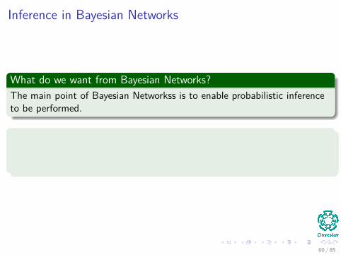
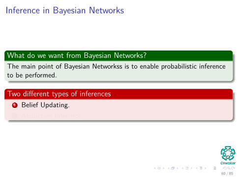
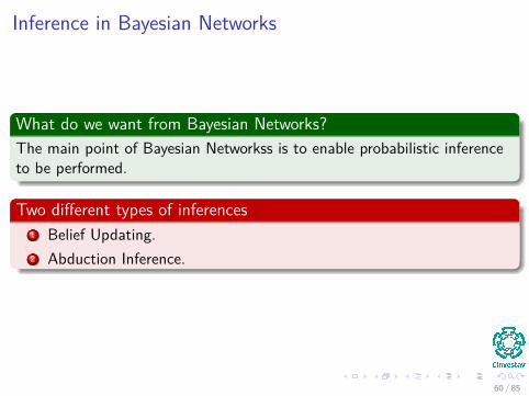
What do we want from Bayesian Networks?The main point of Bayesian Networkss is to enable probabilistic inferenceto be performed.
Two different types of inferences1 Belief Updating.2 Abduction Inference.
60 / 85
Inference in Bayesian Networks
What do we want from Bayesian Networks?The main point of Bayesian Networkss is to enable probabilistic inferenceto be performed.
Two different types of inferences1 Belief Updating.2 Abduction Inference.
60 / 85
Inference in Bayesian Networks
What do we want from Bayesian Networks?The main point of Bayesian Networkss is to enable probabilistic inferenceto be performed.
Two different types of inferences1 Belief Updating.2 Abduction Inference.
60 / 85
Inference in Bayesian Networks
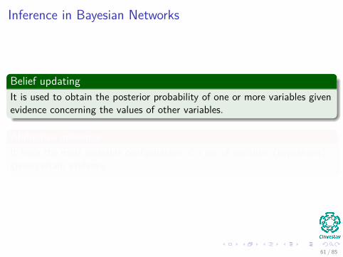
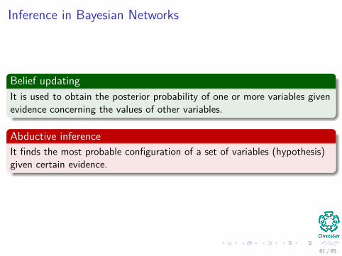
Belief updatingIt is used to obtain the posterior probability of one or more variables givenevidence concerning the values of other variables.
Abductive inferenceIt finds the most probable configuration of a set of variables (hypothesis)given certain evidence.
61 / 85
Inference in Bayesian Networks
Belief updatingIt is used to obtain the posterior probability of one or more variables givenevidence concerning the values of other variables.
Abductive inferenceIt finds the most probable configuration of a set of variables (hypothesis)given certain evidence.
61 / 85
Using the Structure I
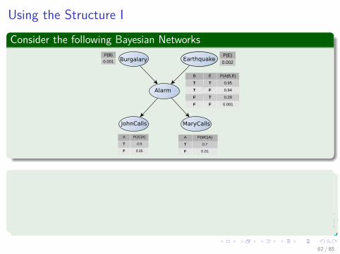
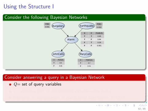
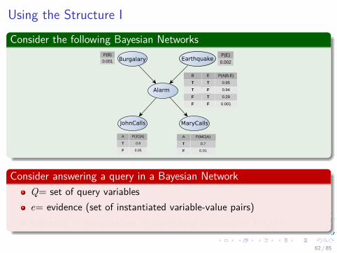
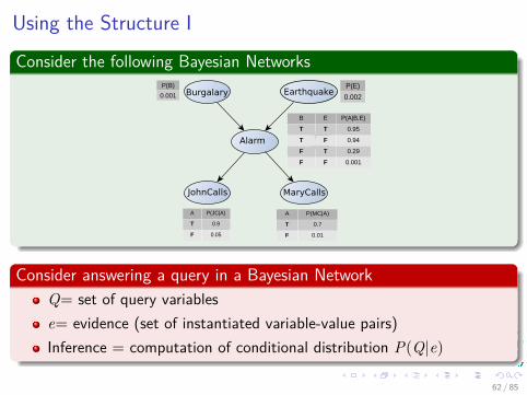
Consider the following Bayesian NetworksBurgalary Earthquake
Alarm
JohnCalls MaryCalls
P(B)
0.001
P(E)
0.002
P(B)
0.001
P(E)
0.002
B E P(A|B,E)
T T 0.95
T F 0.94
F T 0.29
F F 0.001
P(B)
0.001
A P(JC|A)
T 0.9
F 0.05
A P(MC|A)
T 0.7
F 0.01
Consider answering a query in a Bayesian NetworkQ= set of query variablese= evidence (set of instantiated variable-value pairs)Inference = computation of conditional distribution P(Q|e)
62 / 85
Using the Structure I
Consider the following Bayesian NetworksBurgalary Earthquake
Alarm
JohnCalls MaryCalls
P(B)
0.001
P(E)
0.002
P(B)
0.001
P(E)
0.002
B E P(A|B,E)
T T 0.95
T F 0.94
F T 0.29
F F 0.001
P(B)
0.001
A P(JC|A)
T 0.9
F 0.05
A P(MC|A)
T 0.7
F 0.01
Consider answering a query in a Bayesian NetworkQ= set of query variablese= evidence (set of instantiated variable-value pairs)Inference = computation of conditional distribution P(Q|e)
62 / 85
Using the Structure II
ExamplesP(burglary|alarm)P(earthquake|JCalls, MCalls)P(JCalls, MCalls|burglary, earthquake)
SoCan we use the structure of the Bayesian Network to answer such queriesefficiently?
AnswerYES
Note: Generally speaking, complexity is inversely proportional tosparsity of graph
63 / 85
Outline1 History
The History of Bayesian Applications
2 Bayes TheoremEverything Starts at SomeplaceWhy Bayesian Networks?
3 Bayesian NetworksDefinitionMarkov ConditionExample
Using the Markok ConditionRepresenting the Joint DistributionObservations
Causality and Bayesian NetworksPrecautionary Tale
Causal DAGInference in Bayesian NetworksExampleGeneral Strategy of InferenceInference - An Overview
64 / 85
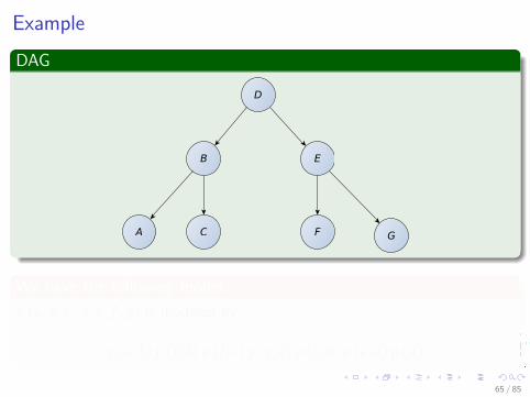
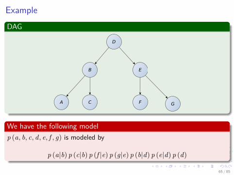
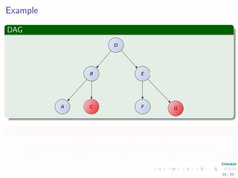
ExampleDAG
D
B E
CA F G
We have the following modelp (a, b, c, d, e, f , g) is modeled by
p (a|b) p (c|b) p (f |e) p (g|e) p (b|d) p (e|d) p (d)
65 / 85
ExampleDAG
D
B E
CA F G
We have the following modelp (a, b, c, d, e, f , g) is modeled by
p (a|b) p (c|b) p (f |e) p (g|e) p (b|d) p (e|d) p (d)
65 / 85
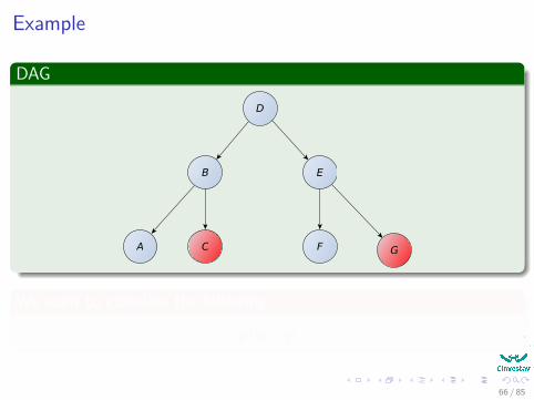
Example
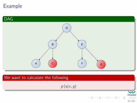
DAG
D
B E
CA F G
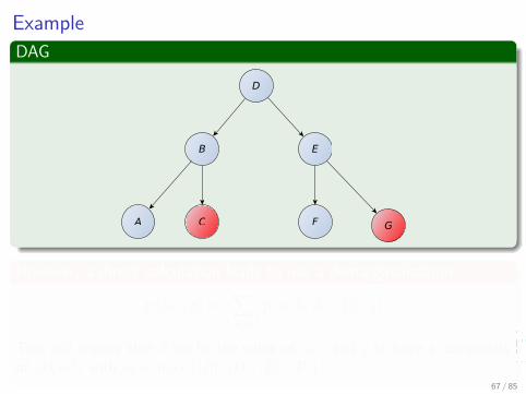
We want to calculate the following
p (a|c, g)
66 / 85
Example
DAG
D
B E
CA F G
We want to calculate the following
p (a|c, g)
66 / 85
ExampleDAG
D
B E
CA F G
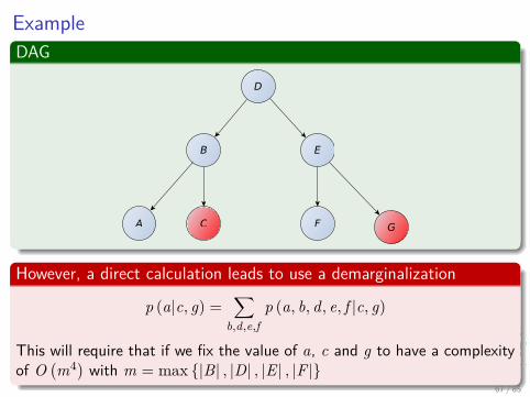
However, a direct calculation leads to use a demarginalization
p (a|c, g) =∑
b,d,e,fp (a, b, d, e, f |c, g)
This will require that if we fix the value of a, c and g to have a complexityof O
(m4) with m = max {|B| , |D| , |E | , |F |}
67 / 85
ExampleDAG
D
B E
CA F G
However, a direct calculation leads to use a demarginalization
p (a|c, g) =∑
b,d,e,fp (a, b, d, e, f |c, g)
This will require that if we fix the value of a, c and g to have a complexityof O
(m4) with m = max {|B| , |D| , |E | , |F |}
67 / 85
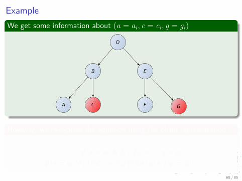
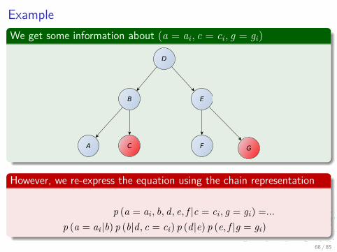
ExampleWe get some information about (a = ai , c = ci , g = gi)
D
B E
CA F G
However, we re-express the equation using the chain representation
p (a = ai , b, d, e, f |c = ci , g = gi) =...
p (a = ai |b) p (b|d, c = ci) p (d|e) p (e, f |g = gi)
68 / 85
ExampleWe get some information about (a = ai , c = ci , g = gi)
D
B E
CA F G
However, we re-express the equation using the chain representation
p (a = ai , b, d, e, f |c = ci , g = gi) =...
p (a = ai |b) p (b|d, c = ci) p (d|e) p (e, f |g = gi)
68 / 85
Example
DAG
D
B E
CA F G
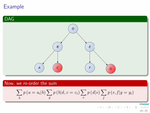
Now, we re-order the sum∑b
p (a = ai |b)∑
dp (b|d, c = ci)
∑e
p (d|e)∑
fp (e, f |g = gi)
69 / 85
Example
DAG
D
B E
CA F G
Now, we re-order the sum∑b
p (a = ai |b)∑
dp (b|d, c = ci)
∑e
p (d|e)∑
fp (e, f |g = gi)
69 / 85
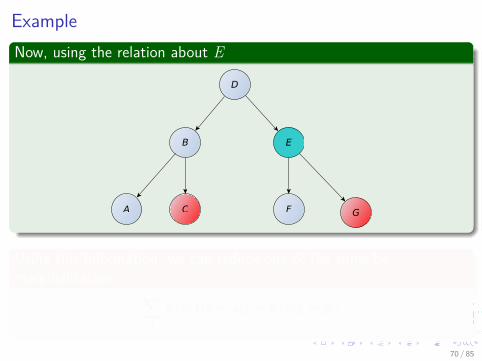
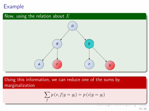
ExampleNow, using the relation about E
D
B E
CA F G
Using this information, we can reduce one of the sums bymarginalization ∑
fp (e, f |g = gi) = p (e|g = gi)
70 / 85
ExampleNow, using the relation about E
D
B E
CA F G
Using this information, we can reduce one of the sums bymarginalization ∑
fp (e, f |g = gi) = p (e|g = gi)
70 / 85
Example
DAG
D
B E
CA F G
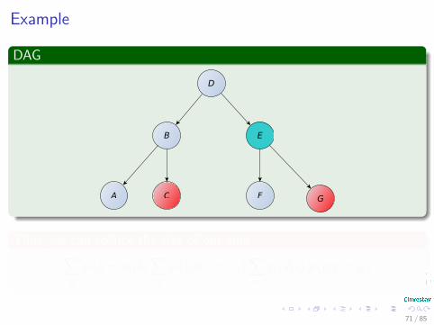
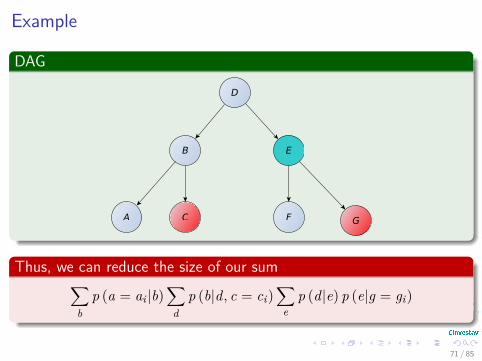
Thus, we can reduce the size of our sum∑b
p (a = ai |b)∑
dp (b|d, c = ci)
∑e
p (d|e) p (e|g = gi)
71 / 85
Example
DAG
D
B E
CA F G
Thus, we can reduce the size of our sum∑b
p (a = ai |b)∑
dp (b|d, c = ci)
∑e
p (d|e) p (e|g = gi)
71 / 85

Example
DAG
D
B E
CA F G
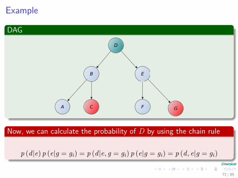
Now, we can calculate the probability of D by using the chain rule
p (d|e) p (e|g = gi) = p (d|e, g = gi) p (e|g = gi) = p (d, e|g = gi)
72 / 85
Example
DAG
D
B E
CA F G
Now, we can calculate the probability of D by using the chain rule
p (d|e) p (e|g = gi) = p (d|e, g = gi) p (e|g = gi) = p (d, e|g = gi)
72 / 85

Example
DAG
D
B E
CA F G
Now, we can calculate the probability of D by using the chain rule∑b
p (a = ai |b)∑
dp (b|d, c = ci)
∑e
p (d, e|g = gi)
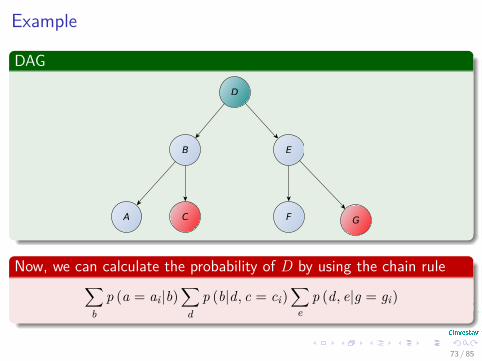
73 / 85
Example
DAG
D
B E
CA F G
Now, we can calculate the probability of D by using the chain rule∑b
p (a = ai |b)∑
dp (b|d, c = ci)
∑e
p (d, e|g = gi)
73 / 85
Example
DAG
D
B E
CA F G
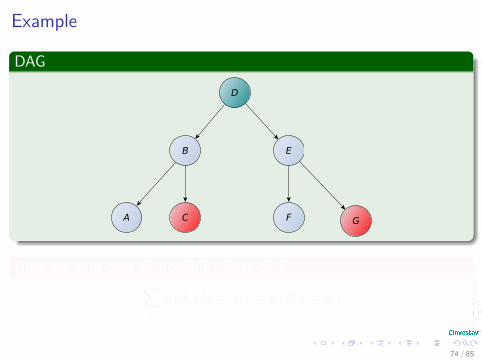
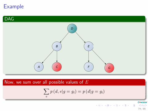
Now, we sum over all possible values of E∑e
p (d, e|g = gi) = p (d|g = gi)
74 / 85
Example
DAG
D
B E
CA F G
Now, we sum over all possible values of E∑e
p (d, e|g = gi) = p (d|g = gi)
74 / 85

Example
DAG
D
B E
CA F G
We get the following∑b
p (a = ai |b)∑
dp (b|d, c = ci) p (d|g = gi)
75 / 85
Example
DAG
D
B E
CA F G
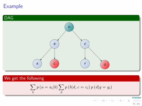
We get the following∑b
p (a = ai |b)∑
dp (b|d, c = ci) p (d|g = gi)
75 / 85
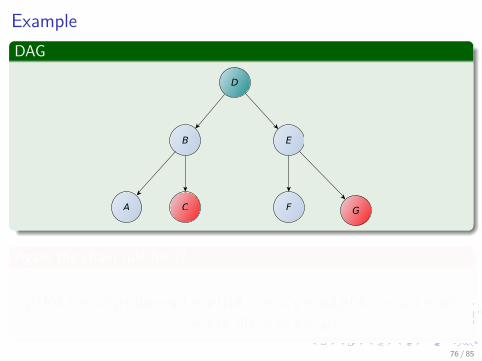
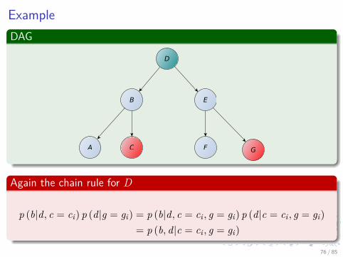
ExampleDAG
D
B E
CA F G
Again the chain rule for D
p (b|d, c = ci) p (d|g = gi) = p (b|d, c = ci , g = gi) p (d|c = ci , g = gi)= p (b, d|c = ci , g = gi)
76 / 85
ExampleDAG
D
B E
CA F G
Again the chain rule for D
p (b|d, c = ci) p (d|g = gi) = p (b|d, c = ci , g = gi) p (d|c = ci , g = gi)= p (b, d|c = ci , g = gi)
76 / 85
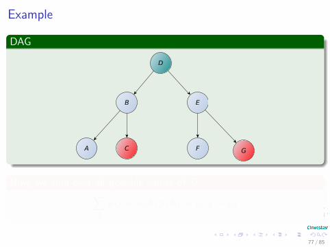
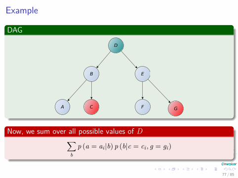
Example
DAG
D
B E
CA F G
Now, we sum over all possible values of D∑b
p (a = ai |b) p (b|c = ci , g = gi)
77 / 85
Example
DAG
D
B E
CA F G
Now, we sum over all possible values of D∑b
p (a = ai |b) p (b|c = ci , g = gi)
77 / 85
Example
DAG
D
B E
CA F G
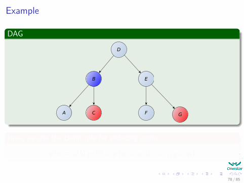
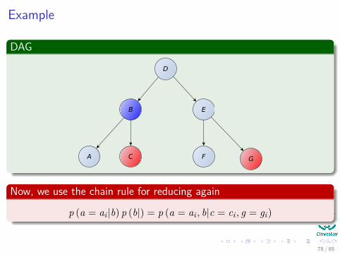
Now, we use the chain rule for reducing again
p (a = ai |b) p (b|) = p (a = ai , b|c = ci , g = gi)
78 / 85
Example
DAG
D
B E
CA F G
Now, we use the chain rule for reducing again
p (a = ai |b) p (b|) = p (a = ai , b|c = ci , g = gi)
78 / 85
Example
DAG
D
B E
CA F G
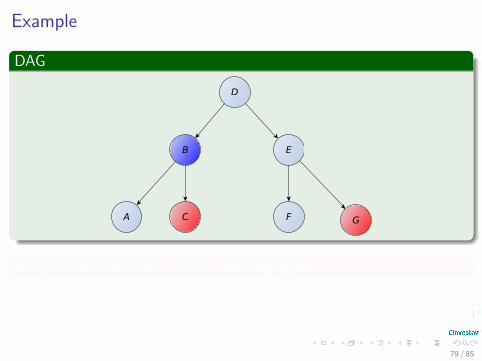
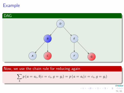
Now, we use the chain rule for reducing again∑b
p (a = ai , b|c = ci , g = gi) = p (a = ai |c = ci , g = gi)
79 / 85
Example
DAG
D
B E
CA F G
Now, we use the chain rule for reducing again∑b
p (a = ai , b|c = ci , g = gi) = p (a = ai |c = ci , g = gi)
79 / 85
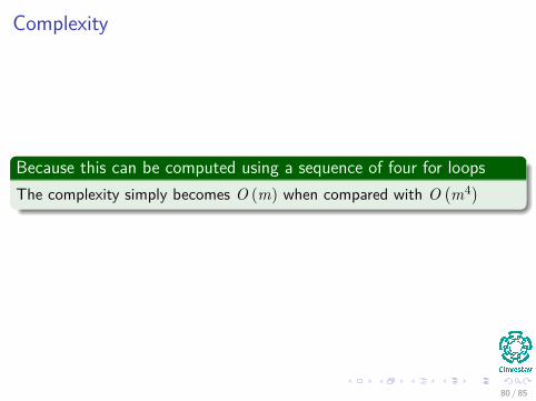
Complexity
Because this can be computed using a sequence of four for loopsThe complexity simply becomes O (m) when compared with O
(m4)
80 / 85
Outline1 History
The History of Bayesian Applications
2 Bayes TheoremEverything Starts at SomeplaceWhy Bayesian Networks?
3 Bayesian NetworksDefinitionMarkov ConditionExample
Using the Markok ConditionRepresenting the Joint DistributionObservations
Causality and Bayesian NetworksPrecautionary Tale
Causal DAGInference in Bayesian NetworksExampleGeneral Strategy of InferenceInference - An Overview
81 / 85
General Strategy for Inference
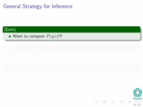
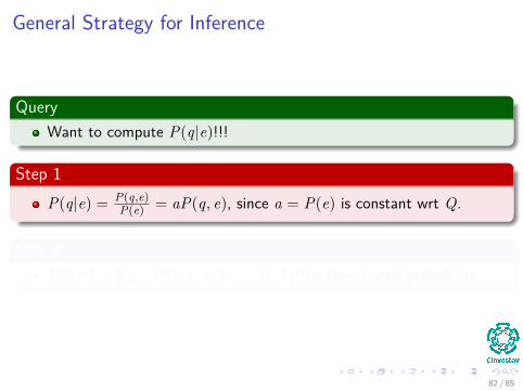
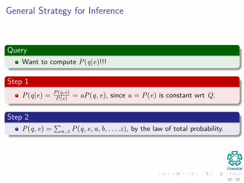
QueryWant to compute P(q|e)!!!
Step 1P(q|e) = P(q,e)
P(e) = aP(q, e), since a = P(e) is constant wrt Q.
Step 2P(q, e) =
∑a..z P(q, e, a, b, . . . .z), by the law of total probability.
82 / 85
General Strategy for Inference
QueryWant to compute P(q|e)!!!
Step 1P(q|e) = P(q,e)
P(e) = aP(q, e), since a = P(e) is constant wrt Q.
Step 2P(q, e) =
∑a..z P(q, e, a, b, . . . .z), by the law of total probability.
82 / 85
General Strategy for Inference
QueryWant to compute P(q|e)!!!
Step 1P(q|e) = P(q,e)
P(e) = aP(q, e), since a = P(e) is constant wrt Q.
Step 2P(q, e) =
∑a..z P(q, e, a, b, . . . .z), by the law of total probability.
82 / 85
General Strategy for inference
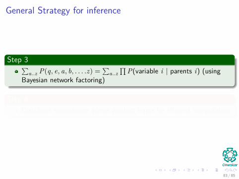
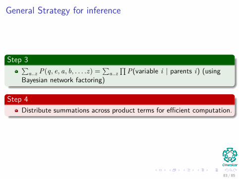
Step 3∑a..z P(q, e, a, b, . . . .z) =
∑a..z
∏P(variable i | parents i) (using
Bayesian network factoring)
Step 4Distribute summations across product terms for efficient computation.
83 / 85
General Strategy for inference
Step 3∑a..z P(q, e, a, b, . . . .z) =
∑a..z
∏P(variable i | parents i) (using
Bayesian network factoring)
Step 4Distribute summations across product terms for efficient computation.
83 / 85
Outline1 History
The History of Bayesian Applications
2 Bayes TheoremEverything Starts at SomeplaceWhy Bayesian Networks?
3 Bayesian NetworksDefinitionMarkov ConditionExample
Using the Markok ConditionRepresenting the Joint DistributionObservations
Causality and Bayesian NetworksPrecautionary Tale
Causal DAGInference in Bayesian NetworksExampleGeneral Strategy of InferenceInference - An Overview
84 / 85
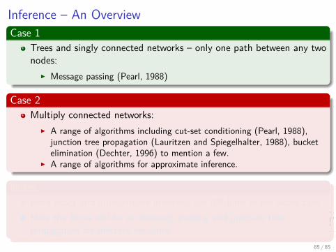
Inference – An OverviewCase 1
Trees and singly connected networks – only one path between any twonodes:
I Message passing (Pearl, 1988)
Case 2Multiply connected networks:
I A range of algorithms including cut-set conditioning (Pearl, 1988),junction tree propagation (Lauritzen and Spiegelhalter, 1988), bucketelimination (Dechter, 1996) to mention a few.
I A range of algorithms for approximate inference.
NotesBoth exact and approximate inference are NP-hard in the worst case.Here the focus will be on message passing and junction treepropagation for discrete variables.
85 / 85
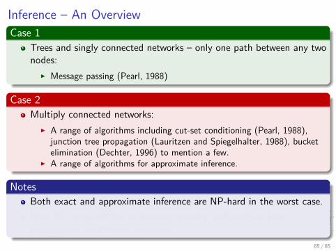
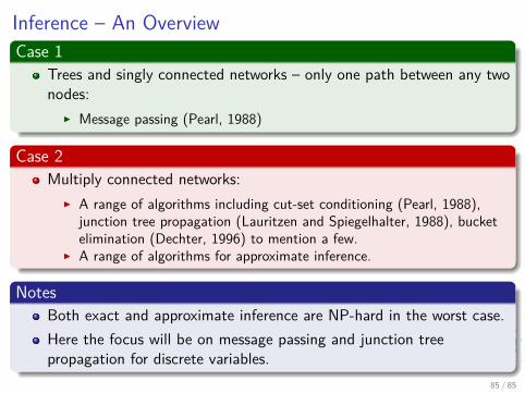