Artificial Dielectric Radio-Frequency Quarter Wave Resonator (Cavity)

Margo A. Batie

Department of PhysicsMassachusetts Institute of Technology

77 Massachusetts AvenueCambridge, MA 02139

Dr. David Wildman and Dr. Robyn Madrak

Accelerator Physics CenterFermi National Accelerator Laboratory

Batavia, IL 60510

Summer Internship in Science and Technology (SIST) ProgramAugust 8, 2012

1

Table of Contents Abstract.......................................................................................................................................3Introduction..................................................................................................................................3

The G-2 Experiment........................................................................................................3About RF Cavities............................................................................................................4

Cavity Number One: The Unloaded Quarter Wavelength Copper Cavity..................................5Cavity Specifications.......................................................................................................5Conclusion.......................................................................................................................6

Cavity Number Two: Loaded Nickel Zinc Ferrite Cavity............................................................6Cavity Specifications.......................................................................................................6Conclusion......................................................................................................................10

Cavity Number Three: Artificial Dielectric Quarter Wavelength Cavity.....................................10Cavity Specifications......................................................................................................1014.5 MHz Cavity..............................................................................................................11

Calculated Results..............................................................................................11Measured Results...................................................................................12Conclusion...............................................................................................12

2.5 MHz Cavity................................................................................................................12Conclusions.....................................................................................................................13

Discussion...................................................................................................................................13Acknowledgements.....................................................................................................................14References..................................................................................................................................15Appendix A: Python Code for SuperFish Data Points................................................................16Appendix B: Data for Altering the 14.5 MHz Cavity to 2.5 MHz................................................18Appendix C:Print out of Resonant Frequency of Network Analyzer..........................................20

2

Abstract The G-2 Experiment requires a high duty factor, high voltage radio-frequency (RF) cavity operating at 2.5 MHz. This cavity will be used in the Recycler Ring to form four 100 nanosecond long proton bunches for muon production. We investigated the possibility of three different types of RF cavities to be used in the G-2 Experiment: one that is unloaded, one with Nickel-Zinc Ferrite rings placed inside, and one with thin copper plates uniformly distributed inside to form an artificial dielectric. Using SUPERFISH, A Computer Program for evaluating RF Cavities with Cylindrical Symmetry, various cavities were modeled to examine the accuracy of measurements and calculations of previously fabricated cavities. What was found was that the artificial dielectric cavity proved to be the best option based on key parameters such as Power Loss, Shunt Impedance and Q values. Introduction The G-2 Experiment

A muon is a fundamental particle classified in the Standard Model for Particle Physics. A muon, similar to an electron, is characterized by its negative charge and ½ spin, however a muon has 200 times the mass of an electron and a mean lifetime of 2.2 microseconds. It is believed that by studying the muon and its spin properties, scientists can explore anomalies that could potentially lead to the discovery of new physics.

Here at the Fermi National Accelerator Laboratory, the overarching theme of all research conducted is the advancement of three frontiers: Energy, Cosmic, and Intensity. The G-2 Experiment hopes to further the boundaries of the Intensity frontier by building on the work of the Brookhaven National Laboratory’s E821 Experiment by gathering more data at higher energies.

Scientists here at Fermilab hope to utilize Fermi’s existing accelerator complex, and reconfigure it so that protons can bombard targets for the purpose of producing muons. My model RF cavity comes into play because FermiLab scientists wish to measure larger quantities of muon interactions, which requires more intensity, in order to increase probabilities thus decreasing uncertainty [1].

For the G-2 Experiment, we need to provide proton bunches that are 100 nanoseconds long, spaced by 400 nanoseconds. These proton bunches are produced by protons driven through the Linear Accelerator (LINAC) at a frequency of 201MHz, giving them energy of 400 MeV. These same proton bunches are injected one after another, into the Booster, a synchrotron 150 meters in diameter, so that they are no longer in phase with the 201 MHz frequency. After the entire stream of protons are inside the Booster, the frequency and corresponding amplitude is increased, so that they gain even more energy and are extracted at 8 GeV [2] and deposited into a 3.3 kilometer storage ring called the Recycler Ring.

It is important to note that in the Booster the protons go from being bunched by the

LINAC’s driving frequency of 201 MHz, to eventually forming new bunches due to the final tuning frequency of the Booster, 52.809 MHz. However, once in the Recycler Ring, the amplitude of this 52.809 MHz frequency is lowered to zero so that the protons are allowed to debunch.

3

My 2.5 MHz cavity will then increase its amplitude and once again cause the protons to be bunched, but now these bunches will be the size and intensity we require so that, using magnets, the beam can be bent and focused at a target to produce muons that are also 100 nanoseconds long. These muons can then be quickly stored in the Muon Storage Ring and studied by G-2 Experimentalists. About RF Cavities

A low frequency cavity is typically a coaxial structure made of copper or aluminum. These materials are used because they have good electrical conductivity properties. At one end, the cavity is shorted, at the other end there is a gap between the end of the inner cylinder and the end of the outer cylinder. This gap is where the maximum voltage appears and where the beam is accelerated.

The way that RF cavities provide charged particles with more energy is by accelerating them via the electromotive force (EMF) or simply the voltage. The force exerted on the particle is related to both the electric field and magnetic field by the Lorentz Force Law:

(1)

The electric field and magnetic field both have a sinusoidal time dependence due to the AC current and the input voltage. In order to exert the maximum force on the particle you want the amplitude of the electric field to be at a maximum as well. That maximum occurs at one quarter of the wavelength of the electric field, and this is why we refer to these cavities as “quarter wave resonators”, because its [resonant] length, , is approximately ¼ of the wavelength. The physical location of that maximum is between the two circular plates at the open end of the cavity,which form a parallel plate capacitor. We define the capacitance between these two plates as the gap capacitance or Cgap .

Cavities can be modeled as an RLC circuit in parallel (so that it may exhibit resonance). A very important term that we use to measure the relative effectiveness of the cavity is the shunt impedance or resistance, Rsh . Rsh is the resistance that the beam current in the cavity sees at resonance, and can be thought of as the resistance which dissipates all of the power lost (Ploss) in the structure when the peak gap voltage (Vgap ) appears across it [3]. Our goal for any cavity is always to minimize how much power is lost.

Another important factor to consider is beam loading. RF cavities are driven by currents, and since current is defined as the flow of charge in a unit of time, the bunches of particles moving through the Recycler Ring form what we call a beam current. So although the RF cavities driving frequency’s amplitude may be turned down to zero, the current provided by the beam can cause an induced voltage from successive bunches causing the succeeding bunches to lose energy and potentially interfere with other bunches. To prevent this occurrence we strive for the least possible Rsh /Q value.

(3)

4

Note: Term in the curly brackets is known as the foreshortening factor, where q=RcCgap=cot(lr) , =2, Rc=LeqCeq and lr is the resonant length of the cavity Leq and Ceq represent the inductance per unit length and capacitance per unit length of the cavity. Again, we want to minimize or reduce the amount of power loss as much as possible, so the bigger Q, the better. Cavity Number 1 Cavity Specifications

For my first model cavity, the resonant length of the cavity was calculated to be 30 meters, using the electromagnetic wave frequency equation.

(4)By setting my resonant length equal to one quarter of the wavelength,, the corresponding foreshortening factor is equal to one. My maximum voltage across the gap is 75 kV, which is the designed gap voltage for each one of our 2.5 MHz Cavities. My inner radius was chosen to be 4 inches, while the outer radius was varied in order to see which result gave me the lowest power loss.

Outer Radius Q Value Rsh Ploss

10 inches 3195.632 223.54 k 12.581 kW

15 inches 5094.956 514.109 k 5.471 kW

20 inches 6548.54 631.934 k 4.451 kW

As you can see the larger the outer radius, the less power we lost. However the problem with this cavity is regardless of what the magnitude of the outer radius is, the resonant length is still too long to fit inside of our equipment drop hatch, which we measured to be 30 feet in length. In order to get this type of cavity to fit inside of the tunnel,the resonant length needs to be foreshortened. By adding a gap capacitance of , I was able to

reduce the resonant length of the cavity, to 26.25 feet. or . While the inner radius remained at 4 inches, the outer radius was set at 15 inches, and the resulting shunt impedance was 107.77 k , which is a factor of 6 lower than what Rsh value we calculated for the full quarter wavelength cavity with the same radii.

We wanted to see how big of an effect altering the inner radius and setting the outer equal to the maximum value (leaving an inch to spare), would have on the shunt impedance of our foreshortened cavity. The optimum value of Rsh was 216.406 k with inner radius set at 2.5 inches and outer at 23 inches, which is still a factor of 2 smaller than our cavity with a foreshortening factor of one. This means that there is still over a 50% decrease in the shunt impedance when you foreshorten our cavity so that it can be lowered into the tunnel.

5

The maximum electric field at the gap is restricted due to a process known as RF

breakdown, or sparking. This relationship between the minimum electric field, E, inside of the cavity at which breakdown will occur, and the frequency is known as the Kilpatrick Limit:

(5)

where For future reference, we wanted to know what would be the absolute minimum gap distance my prospective cavities would require to prevent RF breakdown. Based on the electric field value of

3.78965 for the KP Limit evaluated at 2.5 MHz, and our design peak gap voltage of 75 kV, the minimum gap distance was calculated to be 1.929 centimeters. Conclusion My findings indicate that although it is possible to design a 30 ft long quarter wave copper cavity, it is not an attractive option due to the manufacturing and installation problems resulting from its length and weight. Cavity Number 2 Cavity Specifications

Our next step is to investigate how to alter the resonant length of the cavity without actually changing its dimensions. We resolved that to “shrink” the cavity, we would insert some sort of material between the inner and outer conductor, to reduce the resonant length. The frequency is fixed at 2.5 MHz, since the medium that the wave is travelling in is no longer in vacuum, the wave travels slower, its wavelength is shortened, and its velocity is dependent on permittivity and permeability constants of the medium.

(6)

Since we want the wavelength to be shortened so that the resonant length can be as

close to ¼ of a wavelength as possible, we proposed to fill the entire cavity with whatever material we selected. We prefered for the material to have relatively small losses so that less power would be lost via heat, therefore less work would need to be done cooling the system. We selected Nickel Zinc Ferrite (4M2) due to its extremely high resistivity and low conductivity so that we would not short-circuit the cavity. The properties of Nickel Zinc Ferrite (4M2) are shown in Table 1 and Figure 1:

Symbol Conditions Value Unit

140

6

.1 mT

B250 A/m

mT

250 A/,

mT

DC;

Tc

density

Table 1. 4M2 Material Grade Specifications

Figure 1. Initial Permeability as Function of Temperature

Because we want to be as cost efficient as possible, we decided to reuse the 200

existing Nickel Zinc Ferrite Rings from the Main Injector coalescing cavities here at Fermilab, which are 1 inch thick, with inner and outer diameter 20 cm and 50 cm respectively.

Method

Ferrites possess a peculiar property known as a Curie Temperature, Tc. What is so special about this temperature is that when the ferrite reaches this temperature, it undergoes a sharp change in its magnetic properties, and becomes paramagnetic, or non magnetic [4]. This is not something we want, because if the material’s magnetic permeability, , drastically

7

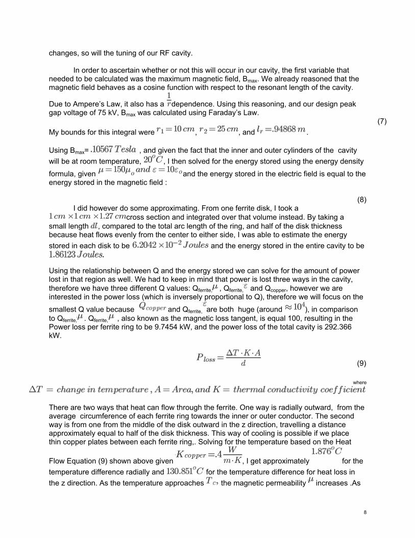
changes, so will the tuning of our RF cavity. In order to ascertain whether or not this will occur in our cavity, the first variable that

needed to be calculated was the maximum magnetic field, Bmax. We already reasoned that the magnetic field behaves as a cosine function with respect to the resonant length of the cavity.

Due to Ampere’s Law, it also has a dependence. Using this reasoning, and our design peak gap voltage of 75 kV, Bmax was calculated using Faraday’s Law.

(7)My bounds for this integral were , , and . Using Bmax= , and given the fact that the inner and outer cylinders of the cavity will be at room temperature, , I then solved for the energy stored using the energy density

formula, given and the energy stored in the electric field is equal to the energy stored in the magnetic field :

(8)I did however do some approximating. From one ferrite disk, I took a

cross section and integrated over that volume instead. By taking a small length , compared to the total arc length of the ring, and half of the disk thickness because heat flows evenly from the center to either side, I was able to estimate the energy stored in each disk to be and the energy stored in the entire cavity to be

Using the relationship between Q and the energy stored we can solve for the amount of power lost in that region as well. We had to keep in mind that power is lost three ways in the cavity, therefore we have three different Q values: Qferrite, , Qferrite, and Qcopper, however we are interested in the power loss (which is inversely proportional to Q), therefore we will focus on the

smallest Q value because and Qferrite, are both huge (around ), in comparison to Qferrite, . Qferrite, , also known as the magnetic loss tangent, is equal 100, resulting in the Power loss per ferrite ring to be 9.7454 kW, and the power loss of the total cavity is 292.366 kW.

(9)

where

There are two ways that heat can flow through the ferrite. One way is radially outward, from the average circumference of each ferrite ring towards the inner or outer conductor. The second way is from one from the middle of the disk outward in the z direction, travelling a distance approximately equal to half of the disk thickness. This way of cooling is possible if we place thin copper plates between each ferrite ring,. Solving for the temperature based on the Heat

Flow Equation (9) shown above given , I get approximately for the temperature difference radially and for the temperature difference for heat loss in the z direction. As the temperature approaches the magnetic permeability increases .As

8

increases, the resonant frequency changes, which is not what we want. Q is defined as:

(10)

Where is our resonant frequency, 2.5 MHz. Based on our RLC representation of an RF cavity, the impedance (which is proportional to the power loss), is a function of the frequency.

The resulting plot has a Lorentzian distribution centered at the resonant frequency. in this case is the change in frequency for the magnitude of the impedance to decrease by a factor

of . Using the value, we see that the frequency can only vary by 25 kHz, which means the magnetic constant can only change 1.5, which correlates to only change in temperature (see Figure 1).. Conclusion Based on our calculations, we see that a ferrite loaded cavity is possible if we place thin copper plates in between each of the ferrite rings.This will result in the temperature difference due to the power lost to be under the the threshold provided by our Q value. However, it is not a good choice for our 2.5 MHz cavity. The reason for this is that although the heat is being lost in a way that the corresponding temperature of each ring is below the Curie Temperature, the magnetic permeability is still increasing. Based on equation (6) we can see that the frequency changes when this happens. As a result we would have to retune the cavity in order to keep up with the changing Also, if is not kept constant, and the tuning frequency deviates too far from the resonant frequency there can be hazardous consequences. When there is too much power, the power has no place to go so it is dissipated in places where it isn’t supposed to. One possible place is the anode of the final power tube of the power amplifier, at a magnitude that exceeds the anode dissipation limit. As a result the anode can melt. Another alarming consequence of unseen power dissipation is less power being put into accelerating the particles and they begin to slow down. When the protons slow, the radius of their trajectory decreases until it eventually crashes into the wall. That much energy being exerted onto the copper surface can be extremely dangerous and damage the tunnel. Cavity #3 Cavity Specifications Our final cavity design is filled with what we call “artificial dielectrics”. The inside of our cavity is lined with circular copper disks, which form multiple parallel plate capacitors inside of our cavity. The purpose of each disk is to lengthen the path of the electric field without actually having to elongate the cavity. Each disk alternates from being attached to the inner cylinder or outer cylinder, leaving a gap of about half an inch in between the adjacent cylinder for the particle to

9

continue its path. 14.5 MHz Cavity A few years back David Wildman, my supervisor, fabricated a prototype Artificial Dielectric RF Cavity. It was 48 inches long, with an inner and outer diameter of 4 inches and 12 inches respectively. Each of the 46 plates was two millimeters thick and separated from one another by a distance of one inch, with a gap distance of one inch as well. My task was to calculate the key parameters such as Q value and Shunt impedance, and then verify those values by physically measuring them, and plotting the cavity in a computer program specially designed for evaluating RF cavities with cylindrical symmetry, called SUPERFISH. Calculated Results

The first step was to find the resonant frequency of this cavity. I assumed that the distance that the electric field travels is equal to one quarter of the wavelength, and this distance can be found by multiplying the number of plates, n, by the distance between each plate which is one inch, and then adding that to the total length of the cavity. Using the wave equation, the resonant length was calculated to be 14.128 MHz. Next I wanted to measure our Q value, in order to find . Q is defined as:

(11)

I calculated our to be and to be using Equation (6). The last term I needed was the equivalent resistance per unit length of the cavity, which includes the line resistance of the inner and outer cylinders (Rline), and the added resistance of each plate. Resistance by definition is:

where (12)

Given that the conductivity coefficient for copper is, , = 3.5 inches, which is the distance to go up one radius of a single disk, and is the average

circumference of each disk, I calculated to be .02577 . Note that to find the total resistivity of all the plates you need to multiply by 92, due to the fact that the equation shown above will only give you the resistivity to travel up one side of one of the 46 plates, and we want both sides of all 46 giving us a factor of 92. The resulting Q value was 759.8 and the corresponding Rsh value was 15.075 k and Ploss= 186.567 kW. Measured Results

10

Using a network analyzer, on the S21 channel, we were able to measure the resonant frequency of our cavity to be at 14.5 MHz. We also detected two other modes, the third and fifth harmonics, at 42.5 MHz and =72.5 MHz. (See Appendix C). The resulting measurements from our Network Analyzer are shown in Appendix C. By using Equation (10), we found the Q value to be approximately 848.

Our next measurement was made possible by a device called a Vector Impedance Meter. What this device does is measure the impedance of a cavity by using Ohm’s Law ( ). The Vector Impedance Meter is able to indicate what the shunt impedance is based on measuring the beam current at the designed peak gap voltage. The resulting measurement for Rsh was 17.1 k . Conclusion

Frequency Rsh Q Ploss

Calculated 14.128 MHz 15.075 k 759.8 186.567 kW

Measured 14.5 MHz 17.1 k 848 164.473 kW

Percent Error 2.56% 12.8% 10.4% 11.8%

Table 2. Parameter Comparison for 14.5 MHz Cavity

When we compare what was calculated to what was measured, the error between the two comes out to be 10%, which is acceptable. 2.5 MHz Cavity Now that we have acceptable results for the artificial dielectric cavity, the next step is to apply what we learned from the 14.5 MHz cavity to produce a 2.5 MHz cavity. To do this we will use Poisson Superfish, a computer program for Evaluating RF Cavities with Cylindrical Symmetry. Superfish requires each of the data points to be written in a certain format. To expedite the plotting process, I wrote a program in Python (See Appendix A). In order to verify the validity of the program we decided to plot the 14.5 MHz cavity in Superfish. The results are shown in Table 3.

Frequency Rsh Q Ploss

Calculated 14.128 MHz 15.075 k 759.8 186.567 kW

Measured 14.5 MHz 17.1 k 848 164.473 kW

SuperFish 14.23 MHz 17.983 k 774.408 165.395 kW

11

Table 3. Parameter Comparison for 14.5 MHz Cavity with Superfish Calculations

Now that we know that our calculations/measurements were correct, we can then use Equation (4) to alter the 14.5 MHz cavity’s dimensions so that our final result is a cavity tuned to 2.5 MHz. The desired frequency is lower than the initial frequency, therefore the resonant length of the final cavity is going to be longer. By varying parameters of the cavity (See Appendix B), the optimal resonant length was calculated to be 104 inches long (8.67 ft), inner radius of 2 inches, outer radius of 12 inches, and disk thickness of 2 mm. The Superfish output is shown in Table 4.

Frequency Rsh Q Ploss

Superfish Simulation

2.49987 MHz 11.6586 k 521.665 55.3828 kW

Table 4. Superfish Results for 2.5 MHz Cavity

Conclusion The 2.5 MHz Cavity modeled in Superfish has the desired frequency and plausible values for the power loss, shunt impedance, and Q value. The dimensions are also reasonable, and coincidentally, are approximately the same size as the existing RF Cavities in the Recycler Ring. Discussion

Frequency Rsh Q Ploss

Unloaded Copper Cavity

2.50 MHz 216.406 k 6112.342 12.996 kW

Ferrite Loaded Cavity

2.50 MHz 9.619 k 100 292.366 kW

Artificial Dielectric

Cavity

2.49987 MHz 11.6586 k 521.665 55.3828 kW

Table 5. The Results of All Three Copper Cavities

My findings are summarized in Table 5. We were able to model three 2.5 MHz Cavities,

however taking into account the effects of the Curie Temperature and level of difficulty to manufacture these cavities, the Artificial Dielectric Quarter Wave Resonator is the best option. The Unloaded copper cavity would be extremely expensive to produce due to its size and weight, while the ferrite cavity, although smaller, would have tuning issues connected to its changing magnetic permeability. The Artificial Quarter Wave Resonator on the other hand, is and will remain tuned to the correct frequency, has a reasonable Q value, and a moderate magnitude for the amount of Power loss.

12

Acknowledgements My research was accomplished at Fermi National Accelerator Laboratory. I would

like to thank Diane Engram, Linda Diepholz, and the entire SIST committee for giving me the opportunity to participate in this program. I would also to like to thank my supervisors, David Wildman and Robyn Madrak, for all of their patience and support throughout the duration of this internship. In addition, I would like to thank my mentors Dave Peterson and Elmie Peoples-Evans for their constant advisement and attention. Finally, I’d like to thank Dr. James Davenport for his assistance in the composition and revision of this paper.

13

References

[1] Fermilab, “The Goal of the New Muon E-989 G-2 Experiment is: ”,The New Muon G-2 Experiment at Fermilab, 2010 [2] B. Worthel, “Introduction” in Booster Rookie Book (3rd Edition), 1998, Available:http://beamdocs.fnal.gov/AD/DocDB/0010/001022/001/Booster%20V3_0.pdf [3] J.E. Griffin, “A Numerical Example of an RF Accelerating System”, in Physics of High Energy Particle Accelerators (Fermilab Summer School, 1981), American Institute of Physics, New York, 1982, p. 564-574 [4] E.C. Snelling, “The Expression of Electrical and Magnetic Properties” in Soft Ferrites: Properties and Applications, 2nd Edition, Butterworth & Co. (1988) p.26-39 [5] Philips Components, “Machined Ferrites”, in Piezoelectric Ceramics Specialty Ferrites: Data HAndbook MA03 (1997), p. 88

14

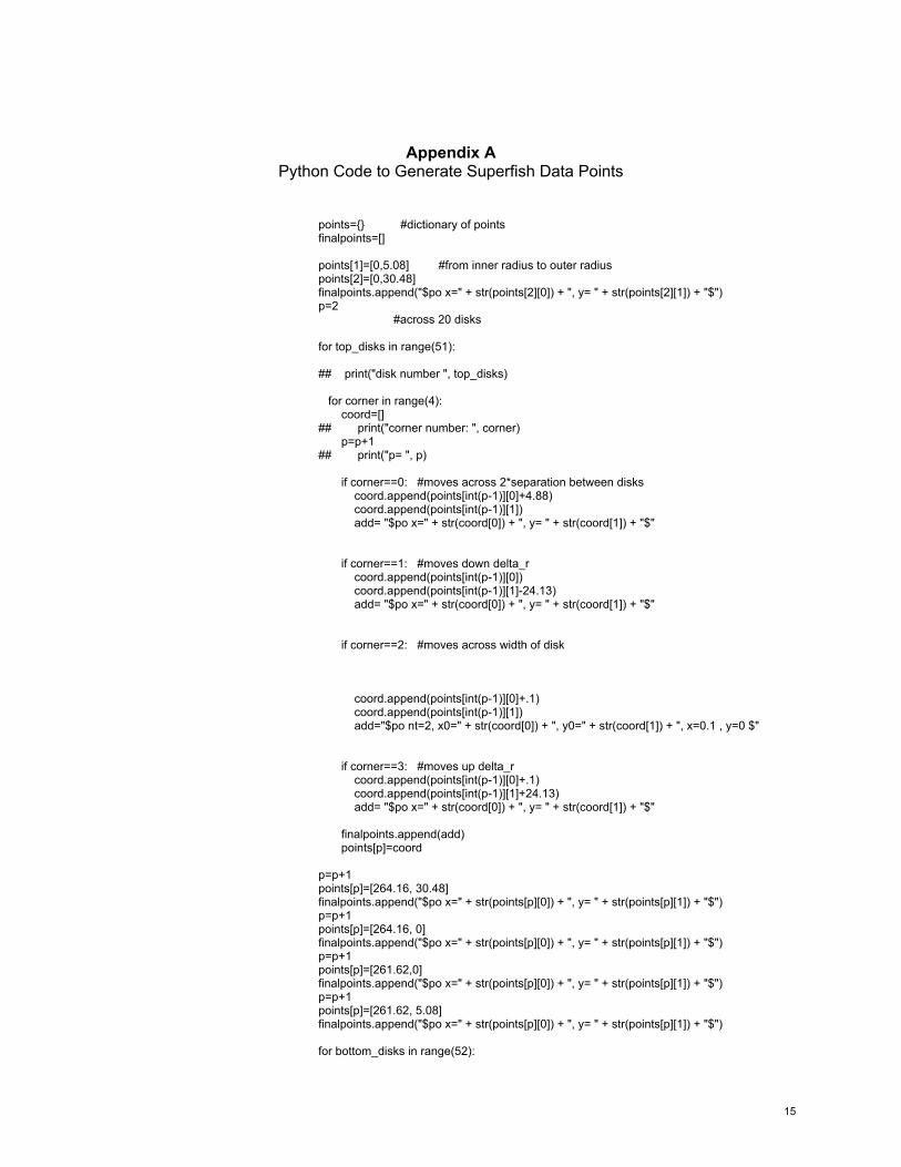
Appendix APython Code to Generate Superfish Data Points

points={} #dictionary of pointsfinalpoints=[] points[1]=[0,5.08] #from inner radius to outer radiuspoints[2]=[0,30.48]finalpoints.append("$po x=" + str(points[2][0]) + ", y= " + str(points[2][1]) + "$")p=2 #across 20 disks for top_disks in range(51): ## print("disk number ", top_disks) for corner in range(4): coord=[]## print("corner number: ", corner) p=p+1## print("p= ", p) if corner==0: #moves across 2*separation between disks coord.append(points[int(p-1)][0]+4.88) coord.append(points[int(p-1)][1]) add= "$po x=" + str(coord[0]) + ", y= " + str(coord[1]) + "$" if corner==1: #moves down delta_r coord.append(points[int(p-1)][0]) coord.append(points[int(p-1)][1]-24.13) add= "$po x=" + str(coord[0]) + ", y= " + str(coord[1]) + "$" if corner==2: #moves across width of disk

coord.append(points[int(p-1)][0]+.1) coord.append(points[int(p-1)][1]) add="$po nt=2, x0=" + str(coord[0]) + ", y0=" + str(coord[1]) + ", x=0.1 , y=0 $" if corner==3: #moves up delta_r coord.append(points[int(p-1)][0]+.1) coord.append(points[int(p-1)][1]+24.13) add= "$po x=" + str(coord[0]) + ", y= " + str(coord[1]) + "$" finalpoints.append(add) points[p]=coord p=p+1points[p]=[264.16, 30.48]finalpoints.append("$po x=" + str(points[p][0]) + ", y= " + str(points[p][1]) + "$")p=p+1points[p]=[264.16, 0]finalpoints.append("$po x=" + str(points[p][0]) + ", y= " + str(points[p][1]) + "$")p=p+1points[p]=[261.62,0]finalpoints.append("$po x=" + str(points[p][0]) + ", y= " + str(points[p][1]) + "$")p=p+1points[p]=[261.62, 5.08]finalpoints.append("$po x=" + str(points[p][0]) + ", y= " + str(points[p][1]) + "$") for bottom_disks in range(52):

15

## print("disk number: ", bottom_disks) for corner in range(4):## print("corner number: ", corner) p=p+1## print("p= ", p) morecoord=[] if corner==3: #moves to the left 2*separation of disk if bottom_disks==51: morecoord.append(points[(p-1)][0]-2.34) morecoord.append(points[(p-1)][1]) add= "$po x=" + str(morecoord[0]) + ", y=" + str(morecoord[1]) + "$" else: morecoord.append(points[(p-1)][0]-4.88) morecoord.append(points[(p-1)][1]) add= "$po x=" + str(morecoord[0]) + ", y=" + str(morecoord[1]) + "$" if corner==0: #moves up delta_r morecoord.append(points[(p-1)][0]) morecoord.append(points[(p-1)][1]+24.13) add= "$po x=" + str(morecoord[0]) + ", y=" + str(morecoord[1]) + "$" if corner==1: #moves left width of disk morecoord.append(points[(p-1)][0]-.1) morecoord.append(points[(p-1)][1]) add= "$po nt=2, x0=" + str(morecoord[0]) + ", y0=" + str(morecoord[1]) + ", x=-0.1 , y=0 $" if corner==2: #moves down delta_r morecoord.append(points[(p-1)][0]-.1) morecoord.append(points[(p-1)][1]-24.13) add= "$po x=" + str(morecoord[0]) + ", y=" + str(morecoord[1]) + "$" finalpoints.append(add) points[p]=morecoord p=p+1points[p]=[0,5.08]finalpoints.append("$po x=" +str(points[p][0]) + ", y=" + str(points[p][1]) + "$") keys=points.keys()for i in range(len(keys)): print(finalpoints[i-1])

16

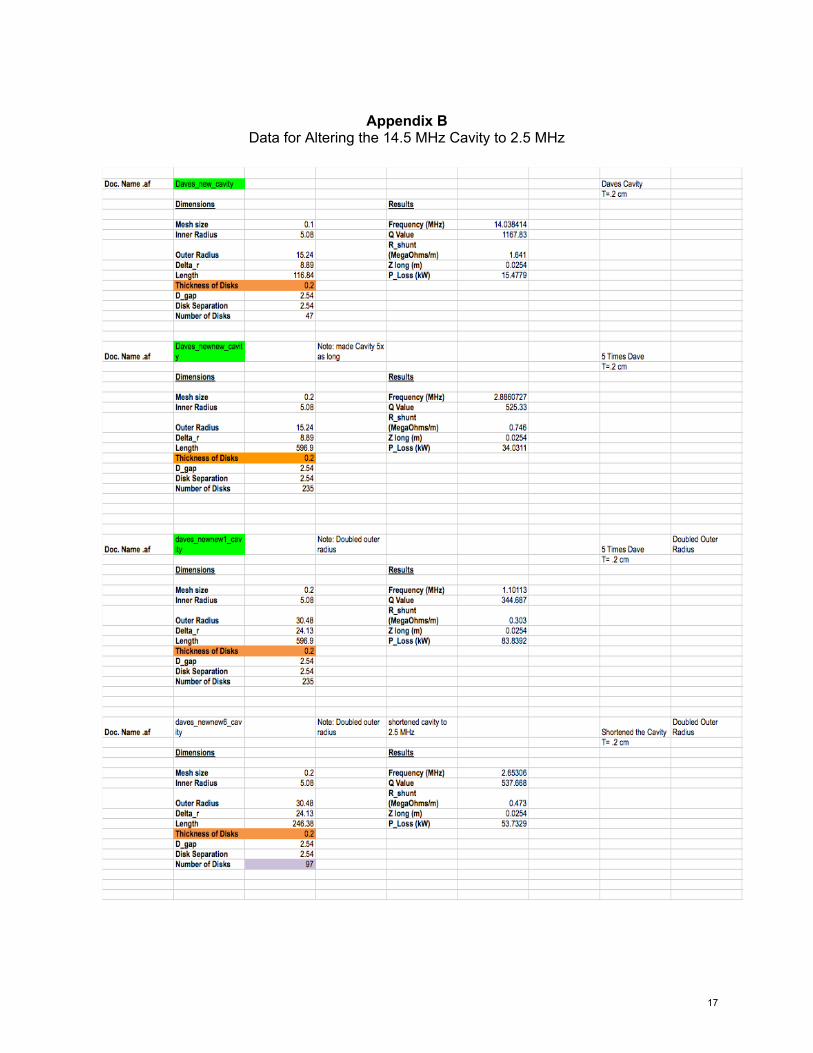
Appendix B

Data for Altering the 14.5 MHz Cavity to 2.5 MHz

17

18

19

Appendix CPrint Out of Resonant Frequencies from Network Analyzer

Frequency=14.325 MHz

20

Frequency=43.555 MHz

21

Frequency=72.553 MHz

22