Artifact Analysis and Removal of Electroencephalographic ... · PDF fileArtifact Analysis and...

Artifact Analysis and Removal ofElectroencephalographic (EEG) Recordings

Yi Dou

A Thesis

in

The Department

of

Concordia Institute for Information Systems Engineering

Presented in Partial Fulfillment of the Requirements

for the Degree of

Master of Applied Science (Quality System Engineering) at

Concordia University

Montreal, Quebec, Canada

March 2017

c© Yi Dou, 2017

CONCORDIA UNIVERSITY

School of Graduate Studies

This is to certify that the thesis prepared

By: Yi Dou

Entitled: Artifact Analysis and Removal of Electroencephalographic

(EEG) Recordings

and submitted in partial fulfillment of the requirements for the degree of

Master of Applied Science (Quality System Engineering)

complies with the regulations of this University and meets the accepted standards with re-

spect to originality and quality.

Signed by the Final Examining Committee:

ChairDr. Jia Yuan Yu

External ExaminerDr. Zhi Chen (BCEE)

ExaminerDr. Jia Yuan Yu

SupervisorDr. Yong Zeng

Co-supervisorDr. Wei-Ping Zhu (ECE)

Approved byRachida Dssouli, ChairDepartment of Concordia Institute for Information SystemsEngineering

2017Amir Asif, DeanFaculty of Engineering and Computer Science

Abstract

Artifact Analysis and Removal of Electroencephalographic (EEG)Recordings

Yi Dou

Electroencephalography (EEG) technique has been widely used in continuous mon-

itoring the brain activities in academic research and clinical applications. In cognitive

neuroscience research, the electrical brain signals can be used to measure mental effort of

subjects. However, the presence of artifacts is a constant problem when recording brain

activities, which will obscure the underlying neural dynamics and therefore make it diffi-

cult to interpret EEG signals accurately. These unwanted signals or artifacts have different

effects depending on their sources of generation. Among them, the motion of the subject

is one of the major contributors to physiological artifacts that causes most of the contam-

inations to the underlying brain activities. It is quite challenging to correct the myogenic

activity from EEG background potentials due to its wide spectral distribution overlapped

with typical bands of brain waves related to cognitive activities, and the spatial distribution

over the entire scalp of human. As such, this thesis focuses on the analysis and removal of

motion artifacts from EEG signals.

The preliminary investigations include the movement-triggered artifact identification

and the analysis of the characteristics of the motion artifact. According to the recorded

video, the contaminated epochs are extracted from the original EEG signals. A set of fea-

tures of the movement-triggered artifacts are proposed based on power spectral density

and wavelet transform. Statistical analysis is performed to distinguish the segments that

iv

contain motions. Two typical methods of artifact removal are then studied, and the effi-

ciency to correct this type of artifact is validated by comparing the extracted features of

non-movement segments and the contaminated segments. The result shows that the tested

artifact removal methods cannot completely remove movement artifacts, which also infers

the potential relation between motion and mental activities.

v

Acknowledgments

First and foremost, I would like to express my profound appreciation to my supervisors

Dr. Yong Zeng and Dr. Wei-Ping Zhu, for their constant guidance and support throughout

the course of my graduate study and research. It would not be possible to complete this

thesis without their insightful advice and inspiration. It is a great fortune to have the oppor-

tunity to work with two such outstanding professors. I am impressed and motivated by their

enthusiasm for the research, and I benefited greatly from their knowledge and wisdom.

I would also like to thank all my colleagues in the Design Lab. It is very fortunate to

be in this friendly research environment and collaborate with all the past and present group

members. Special thanks to Dr. Thanh An Nguyen, for her help and valuable advice in

EEG research. I gratefully acknowledge all the friends that made my time at Concordia

enjoyable.

Last but not the least, I would like to thank my beloved parents, for providing me with

the continuous encouragement and unconditional love in my life. Thank you.

vi

Contents

List of Figures ix

List of Tables xi

1 Introduction 1

1.1 Background and Motivation . . . . . . . . . . . . . . . . . . . . . . . . . 1

1.2 Objective . . . . . . . . . . . . . . . . . . . . . . . . . . . . . . . . . . . 4

1.3 Contribution . . . . . . . . . . . . . . . . . . . . . . . . . . . . . . . . . . 4

1.4 Thesis organization . . . . . . . . . . . . . . . . . . . . . . . . . . . . . . 5

2 Background Material 6

2.1 Electroencephalography (EEG) . . . . . . . . . . . . . . . . . . . . . . . . 6

2.1.1 Lobes of the brain . . . . . . . . . . . . . . . . . . . . . . . . . . 7

2.1.2 Brain waves . . . . . . . . . . . . . . . . . . . . . . . . . . . . . . 9

2.1.3 Event-related potentials (ERPs) . . . . . . . . . . . . . . . . . . . 10

2.2 Artifacts . . . . . . . . . . . . . . . . . . . . . . . . . . . . . . . . . . . . 12

2.2.1 Typical artifacts . . . . . . . . . . . . . . . . . . . . . . . . . . . . 13

2.2.2 Movement-triggered artifact . . . . . . . . . . . . . . . . . . . . . 16

3 Signal Collection and Experimental Setup 18

3.1 Selection of participants . . . . . . . . . . . . . . . . . . . . . . . . . . . 18

vii

3.2 EEG signal recording . . . . . . . . . . . . . . . . . . . . . . . . . . . . . 19

3.3 Movement recording . . . . . . . . . . . . . . . . . . . . . . . . . . . . . 21

3.4 Experiment procedure . . . . . . . . . . . . . . . . . . . . . . . . . . . . . 22

3.5 Data pre-processing . . . . . . . . . . . . . . . . . . . . . . . . . . . . . . 24

4 Movement-triggered Artifact Analysis 26

4.1 EEG data segmentation . . . . . . . . . . . . . . . . . . . . . . . . . . . . 27

4.2 Feature extraction in artifact analysis . . . . . . . . . . . . . . . . . . . . . 31

4.2.1 Power spectral analysis . . . . . . . . . . . . . . . . . . . . . . . . 32

4.2.2 Wavelet analysis . . . . . . . . . . . . . . . . . . . . . . . . . . . 36

4.3 Experimental results . . . . . . . . . . . . . . . . . . . . . . . . . . . . . 40

4.3.1 Results using relative Beta2 power . . . . . . . . . . . . . . . . . . 40

4.3.2 Results using wavelet entropy . . . . . . . . . . . . . . . . . . . . 46

5 Artifact Removal 49

5.1 Canonical correlation analysis (CCA) . . . . . . . . . . . . . . . . . . . . 50

5.2 Independent component analysis (ICA) . . . . . . . . . . . . . . . . . . . 54

5.3 Expermental results . . . . . . . . . . . . . . . . . . . . . . . . . . . . . . 57

5.3.1 CCA . . . . . . . . . . . . . . . . . . . . . . . . . . . . . . . . . 57

5.3.2 ICA . . . . . . . . . . . . . . . . . . . . . . . . . . . . . . . . . . 63

5.4 Discussion . . . . . . . . . . . . . . . . . . . . . . . . . . . . . . . . . . . 68

6 Conclusion and Future Work 69

6.1 Conclusion . . . . . . . . . . . . . . . . . . . . . . . . . . . . . . . . . . 69

6.2 Future Work . . . . . . . . . . . . . . . . . . . . . . . . . . . . . . . . . . 71

Bibliography 73

viii

List of Figures

Figure 2.1 EEG signals from an adult with twenty-one electrodes at various

sites on the brain scalp. . . . . . . . . . . . . . . . . . . . . . . . . . . . . 7

Figure 2.2 Brain lobes. . . . . . . . . . . . . . . . . . . . . . . . . . . . . . . 8

Figure 3.1 64-Ch standard electrode layout. . . . . . . . . . . . . . . . . . . . 20

Figure 3.2 Video recording from the experiment. . . . . . . . . . . . . . . . . 22

Figure 3.3 The location of three web cameras. . . . . . . . . . . . . . . . . . . 23

Figure 3.4 Four stages of the experiment. . . . . . . . . . . . . . . . . . . . . 23

Figure 4.1 The overview of movement-triggered artifact analysis. . . . . . . . . 27

Figure 4.2 Segmentation process and relation between video and EEG. . . . . . 28

Figure 4.3 Three types of segments in the time domain. . . . . . . . . . . . . . 31

Figure 4.4 Power spectral density (PSD) of one subject in a specific movement. 35

Figure 4.5 EEG signal decomposition based on DWT. . . . . . . . . . . . . . . 38

Figure 4.6 A graphical user interface (GUI) for data analysis. . . . . . . . . . . 41

Figure 4.7 An example of PSD in graphical user interface (GUI). . . . . . . . . 42

Figure 4.8 Comparison of means (a) and variances (b) of relative Beta2 power

for each channel. . . . . . . . . . . . . . . . . . . . . . . . . . . . . . . . 43

Figure 4.9 Statistical analysis of relative Beta2 power for all channels. . . . . . 44

Figure 4.10 Statistical analysis of spectral edge frequency (SEF) for all channels

in test period. . . . . . . . . . . . . . . . . . . . . . . . . . . . . . . . . . 45

Figure 4.11 Grand mean of relative Beta2 power in four types of movements. . . 47

ix

Figure 4.12 Comparison of means (a) and variances (b) of wavelet entropy for

three types of segments. . . . . . . . . . . . . . . . . . . . . . . . . . . . . 47

Figure 4.13 Statistical analysis of relative wavelet entropy (RWE) for all channels. 48

Figure 5.1 General framework of signal combination. . . . . . . . . . . . . . . 50

Figure 5.2 Experimental procedure of movement-triggered artifact removal. . . 51


for each channel after applying CCA. . . . . . . . . . . . . . . . . . . . . 58

Figure 5.4 Statistical analysis of relative Beta2 power for all channels after

applying CCA. . . . . . . . . . . . . . . . . . . . . . . . . . . . . . . . . 59


in reconstructed period after applying CCA. . . . . . . . . . . . . . . . . . 60


each channel after applying CCA. . . . . . . . . . . . . . . . . . . . . . . 61

Figure 5.7 Statistical analysis of relative wavelet entropy (RWE) for all chan-

nels after applying CCA. . . . . . . . . . . . . . . . . . . . . . . . . . . . 62


for each channel after applying ICA. . . . . . . . . . . . . . . . . . . . . . 63

Figure 5.9 Statistical analysis of relative Beta2 power for all channels after

applying ICA. . . . . . . . . . . . . . . . . . . . . . . . . . . . . . . . . . 64


in context period (a) and test period (b) after applying ICA. . . . . . . . . . 65


each channel after applying ICA. . . . . . . . . . . . . . . . . . . . . . . . 66

Figure 5.12 Statistical analysis of relative wavelet entropy (RWE) for all chan-

nels after applying ICA. . . . . . . . . . . . . . . . . . . . . . . . . . . . . 67

x

List of Tables

Table 3.1 Number of segments for each subject. . . . . . . . . . . . . . . . . . 24

Table 4.1 Time table of physical movements for segmentation . . . . . . . . . . 30

Table 4.2 P value for colored channels in test period (Beta2). . . . . . . . . . . 45

Table 4.3 P-value for colored channels in test period (SEF). . . . . . . . . . . . 46

Table 4.4 P value for colored channels in test period (RWE). . . . . . . . . . . 48

xi

Chapter 1

Introduction

1.1 Background and Motivation

Electroencephalography is a non-invasive measurement of brain activity, which could

be used to record the electrical activity of brain from the scalp related to cortical activ-

ity. Early in 1920s, Hans Berger first measured the brain activity on human scalp, and

defined the word electroencephalogram for describing brain electric potentials. Also, it is

conjectured that periodic fluctuation of EEG might be related with general cognitive states

of subjects, including arousal and consciousness. Over the past several years, researchers

have actively studied EEG to understand the cognitive process.

Recently, a variety of imaging techniques have been applied for studying brain func-

tions of human, such as magnetic resonance imaging (MRI), positron emission tomography

(PET) and single photon emission computed tomography (SPECT). These measurements

can provide good spatial resolution of two or three dimensional images. However, EEG is

still a powerful and frequently-used tool in modern medicine field and academia to mea-

sure brain activity with its own advantages. Above all, EEG has a relative high temporal

resolution for data processing compared with above-mentioned imaging techniques, which

1

is essential for real-time monitoring. Besides that, the total cost of EEG recording instru-

mentation is extremely lower than others, with the use of electrodes, conductive media and

computer software for signal storage and analysis (Teplan, 2002).

To trace the bioelectric potentials in brain, electrodes are used to place directly on

human skin. When the nerve or muscle cells are activated, ionic potentials are produced.

The effect of electrodes is to convert these ionic potentials into electrical potentials which

can be measured. Since EEG is obtained directly from the scalp surface, this procedure

can be applied repeatedly to normal adults, children and patients nearly without risk and

limitation.

EEG signal has a wide range of applications in modern medicine. Since EEG contains a

lot of information reflecting the state of body health and different physiological states of the

brain, it is one of the most commonly-used tools for monitoring the neurological disorders,

such as epileptic seizures (McGrogan et al., 1999). In order to detect the time when the

epileptic activity occurs, long-term monitoring is always employed. Apart from that, other

applications include the evaluation of brain activity during human sleep and severity of

sleep disorders (Carskadon & Rechtschaffen, 2000) (Berka et al., 2005), the assessment

of mental workload (Gevins et al., 1998) (Gevins & Smith, 2003) (Berka et al., 2007) and

brain-computer interfaces (BCI) (Wolpaw & McFarland, 2004).

No matter which fields the EEG signals are applied to, it is critical to ensure the high

quality of the recorded signals. Normally, the neural EEG signals are in the range of micro

volts, and it can be masked by undesired potentials mostly generated from non-cerebral ori-

gin, which are called artifacts. In academic studies and clinical applications, the presence of

artifact is a constant problem during the recording of brain activity. These unwanted signals

always have different forms of effects depending on the sources of the artifacts. Among

all types of artifacts, electrooculography (EOG) and electromyography (EMG) artifacts are

two major contributors of physiological artifacts that cause most of contaminations to the

2

underlying brain activity.

As reviewed in (Fatourechi, Bashashati, Ward, & Birch, 2007), the consideration of

EMG and/or EOG artifacts are not reported in most BCI papers published until 2006, and

the number of studies that did not report EMG artifacts is higher than that of EOG.

With the help of a series of electrodes settled close to the eyes as reference channels,

the electrooculogram (EOG) can be recorded for dealing with eye-movement artifacts. The

most common technique for ocular artifact removal is based on linear combination and

regression (Croft & Barry, 2000). Furthermore, it is argued that the error in the subtraction

phase is small relative to the main EOG correction (Croft & Barry, 2002).

However, since there is no reference channel for EMG artifact, it is particularly chal-

lenging to correct muscle artifact, which has high amplitude, broad frequency distribu-

tion and variable topographical distribution, as investigated in (Goncharova, McFarland,

Vaughan, & Wolpaw, 2003). In clinical practice, the entire affected segments of data would

be rejected in most circumstances, while it will definitely lead to a considerable information

loss.

There exists a variety of methods for artifact separation and removal. By using simple

filtering techniques, such as band pass filters, the separation could be accomplished in

frequency domain. However, since the frequency of artifact and the desired signal are

always overlapped in actual situations, alternative techniques should be applied.

Methods of blind source separation (BSS) are currently utilized in signal processing for

removing artifact. Based on the assumption that the neural activity and artefactual signal

are not systematically co-activated, the separation is performed after the transformation of

the recorded EEG signals into a set of source components. There are several algorithms to

perform BSS, including canonical correlation analysis (CCA) (Clercq, Vergult, Vanrumste,

Paesschen, & Huffel, 2006) and independent component analysis (ICA) (Jung et al., 2000),

which are employed in this thesis for artifact removal.

3

1.2 Objective

The objective of this thesis is two-fold. The first objective is to analyze the artifacts

generated from the voluntary motions of subjects during a cognitive task, and investigate

the characteristics of artefactual segments through feature extraction, which is performed

by the Fast Fourier Transform (FFT) method in the frequency domain and the Wavelet

Transform (WT) in the time-frequency domain. The second objective is to remove this

type of artifacts in EEG recordings by two existing artifact removal techniques, and validate

their performances.

1.3 Contribution

The contributions of this thesis are described below.

• A comprehensive literature review of the artifacts in EEG signals and the state of the

art in artifact removal techniques are presented.

• A guideline is provided to extract the EEG segments contaminated by movement-

triggered artifacts based on the video recording of the experiments of subjects.

• A graphic user interface is developed to extract the features for movement-related

signal analysis, and distinguish the statistical differences when movement occurs in

scalp map.

• Two typical techniques of artifact removal are attempted, and the performances are

evaluated according to feature extraction results.

4

1.4 Thesis organization

The rest of this thesis consists of the following five chapters. The content of each

chapter is described below:

Chapter 2 introduces the basic background of the physiological signal in human brain,

which is called electroencephalography (EEG). The relevant signal waves and artifacts are

also described with the commonly used classification.

Chapter 3 provides a brief introduction of the cognitive experiment in 2015, which mea-

sures the physiological signals concerning mental effort during design activities. With the

help of video recording, all the useful information was collected for movement-triggered

artifact analysis.

Chapter 4 analyzes the movement-triggered EEG signals generated from the cognitive

experiment, as presented in segmentation section and feature extraction section. For manual

screening and marking of artifacts, a set of criteria are proposed, which will be used to

extract the affected segments from the EEG recording. At the same time, the comparison

of different features is also presented.

Chapter 5 focuses on the study of various methods for artifact removal. Among these

techniques, two of them are described in detail, namely canonical correlation analysis

(CCA) and independent component analysis (ICA). Furthermore, the selection of artifact

components is studied in this chapter. A comparison of results is also presented.

Chapter 6 summarizes the research results of this thesis and suggests some topics for

future work.

5

Chapter 2

Background Material

2.1 Electroencephalography (EEG)

In cognitive neuroscience research, it is generally known that there exists a modular

organization in the brain. These discrete units of modules are functionally constructed,

and they are interact to the generation of mental activities. The aim of this research is

to investigate the neural basis of cognition and figure out how the different areas of brain

support cognitive functions (Gazzaniga, 1989). To this end, the anterior cingulate cortex

(ACC) has been discussed, and it is suggested that ACC has a relationship with mental

effort by using event-related potentials (Mulert, Menzinger, Leicht, Pogarell, & Hegerl,

2005). Apart from that, the dynamic of ACC activity can be investigated by functional

imaging techniques.

Design can usually be considered as a high level cognitive ability. The design activity

can be studied by measuring physiological signals as well, such as functional magnetic res-

onance imaging(fMRI) (Alexiou, Zamenopoulos, Johnson, & Gilbert, 2009) and electroen-

cephalography (EEG). During cognitive processes, electrical brain signals can be applied

to identify mental design activities (Nguyen & Zeng, 2012) and measure mental effort of

subjects (Nguyen & Zeng, 2014). Various EEG features are introduced to reflect mental

6

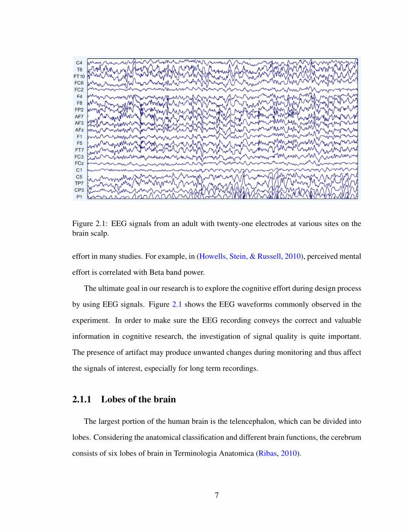
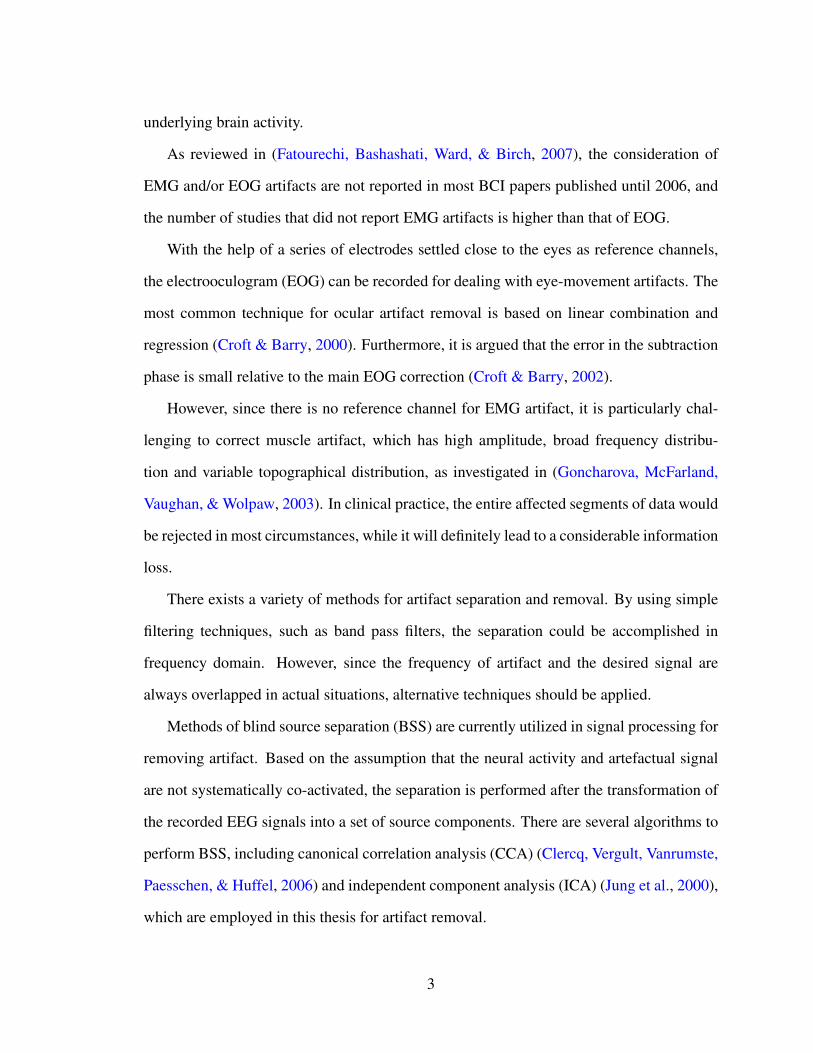
Figure 2.1: EEG signals from an adult with twenty-one electrodes at various sites on thebrain scalp.

effort in many studies. For example, in (Howells, Stein, & Russell, 2010), perceived mental

effort is correlated with Beta band power.

The ultimate goal in our research is to explore the cognitive effort during design process

by using EEG signals. Figure 2.1 shows the EEG waveforms commonly observed in the

experiment. In order to make sure the EEG recording conveys the correct and valuable

information in cognitive research, the investigation of signal quality is quite important.

The presence of artifact may produce unwanted changes during monitoring and thus affect

the signals of interest, especially for long term recordings.

2.1.1 Lobes of the brain

The largest portion of the human brain is the telencephalon, which can be divided into

lobes. Considering the anatomical classification and different brain functions, the cerebrum

consists of six lobes of brain in Terminologia Anatomica (Ribas, 2010).

7

Figure 2.2: Brain lobes.

There are four major lobes of the cerebral cortex in human brain, frontal, parietal, tem-

poral and occipital lobe, as shown in Figure 2.2. The locations and functions are introduced

as follows:

• Frontal lobe:

The space at the front of cerebral hemisphere is called frontal lobe, which usually

contains dopamine-delicate neurons, and it is involved in attention, short-time mem-

ory tasks, planning and motivation.

• Parietal lobe:

The parietal lobe is located above the occipital lobe and behind the frontal lobe. The

sensory information in different modalities is collected in this area, including spatial

sense and sensory input for the skin. In addition, several regions in parietal lobe play

an important role in language processing.

• Temporal lobe:

8

The region beneath the lateral fissure on two sides of cerebral hemispheres is called

temporal lobe. It is associated with visual memories, language comprehension, and

emotion association.

• Occipital lobe:

Since the occipital lobe contains most of the anatomical region of visual cortex, it

is considered as the visual processing center of the brain. Extrastriate regions are

related to different tasks, such as visuospatial processing, motion perception and

color differentiation.

2.1.2 Brain waves

In order to provide a constant recording of electrical activity of the brain for brain

researchers and clinical experts, two basic parameters: amplitude and frequency are used

to describe EEG. Some of the EEG patterns are quite reliable for visual inspection. In

general, there are five typical brain waves classified by different frequency ranges, and

these rhythms are identified by Greek letters respectively as δ (delta), θ (theta), α (alpha),

β (beta) and γ (gamma). Berger introduced the alpha and beta waves in 1929. Jasper and

Andrews named the gamma wave in 1938. Delta and theta rhythms were introduced by

Walter (1953).

Delta activity refers to EEG activity in the 0.5-4 Hz. It is mostly associated with EEG-

synchronized sleep in humans. In the first years of life for human infants, the predominant

frequency is also delta rhythm.

Theta activity can be seen with a low frequency range of 4-8 Hz. Schacter (1977)

indicates that theta activity is related to two psychological events. The first one is a low

level of alertness in hypnagogic and sleep deprivation states. On the other hand, in problem-

solving and perceptual processing, theta is associated with active and efficient processing.

Alpha activity occurs over the posterior regions of the head, and in most of individuals

9

when they are awake and relaxed. The alpha rhythm consists of relative high voltage,

which is normally less than 50 V, over the occipital areas within the range of 8 to 13 Hz.

The presence is related to physical relaxation with eye closed and relative mental inactivity

(Niedermeyer & da Silva, 2005).

The usual waking rhythm of the brain is beta wave, which is related to active thinking,

active attention and solving concrete problems in normal adults. Normally, beta wave has

low-voltage variations with the range of 13 to 30 Hz.

A higher frequency range from 30 to 70 Hz or more with lower voltage variations is

gamma rhythm.

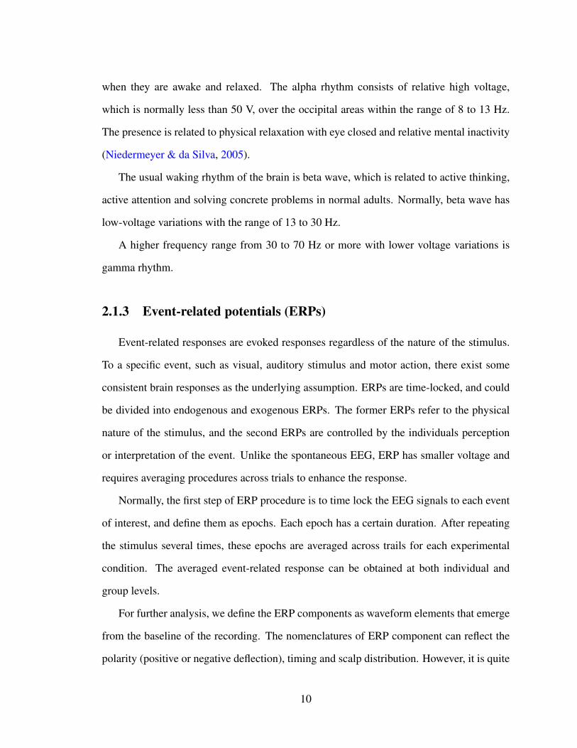
2.1.3 Event-related potentials (ERPs)

Event-related responses are evoked responses regardless of the nature of the stimulus.

To a specific event, such as visual, auditory stimulus and motor action, there exist some

consistent brain responses as the underlying assumption. ERPs are time-locked, and could

be divided into endogenous and exogenous ERPs. The former ERPs refer to the physical

nature of the stimulus, and the second ERPs are controlled by the individuals perception

or interpretation of the event. Unlike the spontaneous EEG, ERP has smaller voltage and

requires averaging procedures across trials to enhance the response.

Normally, the first step of ERP procedure is to time lock the EEG signals to each event

of interest, and define them as epochs. Each epoch has a certain duration. After repeating

the stimulus several times, these epochs are averaged across trails for each experimental

condition. The averaged event-related response can be obtained at both individual and

group levels.

For further analysis, we define the ERP components as waveform elements that emerge

from the baseline of the recording. The nomenclatures of ERP component can reflect the

polarity (positive or negative deflection), timing and scalp distribution. However, it is quite

10

difficult to get ERP component, because the voltage deflections of the resulting ERP reflect

the sum of several relatively independent underlying to latent components, and it is difficult

to isolate the latent components. Thus, a set of rules were proposed by Luck (2005) to

avoid misinterpreting the relationship between the observable peaks and the underlying

components.

Event-related potential (ERP) technique has a better performance for studying percep-

tion and attention than other techniques, such as fMRI and PET. Since ERPs have a precise

temporal resolution based on the sample rate, the brain activity can be measured on a scale

of tens of milliseconds, as well as many aspects of attention and perception in operation

(Woodman, 2010).

Early in 1951, Bates recorded cerebral potentials associated with voluntary muscular

movements by superimposing EEG tracing. With the EMG signals recorded by surface

electrodes to obtain the onset of motor contraction, he found a small potential change

after the onset of electromyogram. Later, by repeating movements and averaging EEG

segments off-line, Kornhuber and Deecke (1965) found the Bereitschaftspotential (BP) or

readiness potential (RP) preceding the EMG onset. Two more components were then iden-

tified as pre-motion positivity and motor potential, just before the onset of EMG in (Deecke,

Scheid, & Kornhuber, 1969). Since then, the interest for movement-related cortical poten-

tials (MRCP) has widely increased.

Pre-movement activity refers to the time of movement preparation when the subject is

going to perform afterwards, but no muscle movement is detectable. Study shows that BP

usually starts around 2 s before the movement onset in (Shibasaki & Hallett, 2006). The

changes before movements and brain status could provide useful information in practical

applications. For example, in brain computer interfaces (BCIs), BP can predict the intention

and direction of the upcoming movement, and even determine the future moving limb, as

reviewed in (Ahmadian, Cagnoni, & Ascari, 2013).

11

However, movement-triggered artifact analysis is not a typical ERP problem in this

thesis, since the movements generated by the subjects is not repeatable. In addition, the

magnitude of muscle movement artifact is greater than the ERP.

2.2 Artifacts

According to the International Federation of Clinical Neurophysiology (IFCN), artifact

is defined as any potential difference due to an extra-cerebral source, recorded in EEG

tracing. Contamination of the EEG signals by artifact is a well-recognized problem for

clinical and experimental electroencephalography. Since EEG activity would be obscured

by artifact, which will lead to misinterpretation and false conclusions (Klass, 1995).

It is always a challenge to deal with artifact for the academic studies, both excellent

training and considerable experience are required. The first thing is to recognize the exis-

tence of artifacts, and then, identify the type and determine the source. After that, eliminate

the artifact if possible. However, artifacts may have similar parameters in rhythmicity, fre-

quency and recurrence compared to the recorded potentials of cerebral origin. So it would

become quite difficult to figure out the distinction between artefactual and cerebral electri-

cal activity (Brittenham, 1974).

Since the neural EEG signals are always in the range of micro volts, it can be easily cov-

ered with unwanted artifacts. Typically, based on their origin, the artifact can be divided

into two categories, physiological and non-physiological artifacts. The sources of physi-

ological artifacts are the non-neural activities of the subjects, such as eye movement and

muscle activities, which can hardly be avoided during monitoring. While the non-neural

artifact arises from outside of the body, such as equipment and environment. This technical

artifact can be reduced by proper attachment of the electrodes in a controlled environment

(Anderer et al., 1999). Therefore, most of the algorithms of EEG artifact removal are de-

veloped to reduce the physiological artifacts.

12

In the brain computer interface (BCI) research, electrooculography (EOG) and elec-

tromyography (EMG) artifact are the most commonly detected sources of physiological

artifacts.

Many studies have reported that EMG activities could affect the neurological phenom-

ena used in a BCI system. For example, in (McFarland, Sarnacki, Vaughan, & Wolpaw,

2005), early target-related EMG artifact is presented during initial BCI training, which

would be associated with unsuccessful EEG control. It is suggested that the EMG contam-

ination should be considered in the studies using EEG rhythms. Indeed, the characteristic

of frontalis and temporalis muscle EMG is described in (Goncharova et al., 2003).

2.2.1 Typical artifacts

In this section, some common types of artifacts are briefly reviewed.

Electroculogram (EOG)

Electroculogram is the electrical activity produced by eye movement, which has a large

effect on EEG recording. The potential difference between the cornea and retina can be

altered by eye movement, which exists not only in the wake state, but also during sleep.

The strength of EOG mostly relies on the electrode close to eyes and the direction of eye

movement (horizontal or vertical). In addition, the potential difference could be influenced

by blinking, which is generated by the muscle movement of eye lid. This type of ocular

activity produces a different waveform, and it may only occur during the wake periods. The

blinking artifact has a high frequency and the amplitude is significantly larger in the frontal

electrodes.

For artifact processing, EOG signals can be measured by using reference electrodes

placed near the eye in practice. As a common type of artifact, EOG can present serious

complication in EEG analysis due to the close proximity to the brain (Sornmo & Laguna,

13

2005).

Electromyogram (EMG)

Different parts of the body can be moved by the contraction of muscle tissue. These

muscles are categorized as skeletal, smooth and cardiac muscles. Electromyogram (EMG)

reflects the electrical activities of skeletal muscles, where the action potentials propagate

between the nervous systems and the muscles. Normally, a needle electrode or non-

invasively electrode could be used to measure myoelectric signals. In research practice,

with the help of surface electrodes on the skin, the surface EMG is mostly investigated.

The recording of surface EMG can be contaminated by different types of noise, such as

electrode motion artifact, which will hinder signal quality (Sornmo & Laguna, 2005).

Cranial EMG have several properties which are responsible for the pernicious effects on

the EEG background activity. First of all, it was shown that the EMG has a broad frequency

distribution from 0 to >200 Hz (Goncharova et al., 2003), which means that EMG activity

affects all classic EEG bands, including alpha, beta and delta bands. For topographical

distribution of EMG, as the strength of muscle contraction increases, EMG effect comes to

widespread and involves the entire scalp. Moreover, EMG obscures experimental manip-

ulations in time domain, such as facial EMG, which is sensitive to cognitive and affective

processes (Cohen, Davidson, Senulis, Saron, & Weisman, 1992).

The timing of muscle contraction is normally identified by using surface electromyo-

graphic (EMG) signals. Research from Conforto, D’Alessio, and Pignatelli (1999) indi-

cated that the information acquired from this type of signal is always influenced by motion

artifacts, and this disturbing effect of artifacts obstructs the correct detection and further

analysis. During the non-invasive myoelectric signal recording, muscular contractions lead

to the movements of electrodes, which allocate most of the artifact contribution.

14

Electrocardiogram (ECG)

The electrical activity of the heart is measured by electrocardiogram (ECG). Compared

to the EEG signals, the amplitude of cardiac activity is lower on the scalp. The ECG inter-

ference depends on the electrode positions for certain body shapes. The normal heartbeats

can usually be characterized in a repetitive, regularly occurring waveform pattern, which is

helpful to reveal the presence of ECG artifact. However, when ECG is barely visible in the

background EEG signals, this type of artifact may sometimes be mistaken for epileptiform

activity.

Like the eye-related artifacts as we mentioned above, the ECG can be measured in-

dependently by setting several reference electrodes aside cerebral activity, which is much

easier to correct EEG signals.

Technologic artifacts

As an uncontrolled/unwanted variation in the experimental setup, technologic artifacts

can be generated in the data acquisition system connecting subjects to the EEG instrument,

which includes the electrode, the lead, the electrode-scalp interface, the jack plug and the

input cable. This type of experimental artifact could be reduced by proper procedure and

planning, but it is nearly impossible to avoid or eliminate completely.

One possible source of artifact is the electrode wire which connects the electrode to the

acquisition equipment. Owing to the insufficient shielding in practice, the currents flowing

from nearby powerlines or electrical devices generate electromagnetic fields. Thus, 50/60

Hz powerline interference contaminates the EEG signals.

The movement of electrodes could change the DC contact potential and produce an arti-

fact named as electrode-pop artifact. This technical artifact may occur not only in the EEG

signals, but also in any bioelectric signals measured on the body surface. The electrode-pop

artifact is mostly behaved as an abrupt change in the baseline level.

15

Motion by subjects could alter the position of the electrode on the scalp. There exists

a variation of distance between the recording electrode and the skin, then a corresponding

change in the electrical coupling is created and results in signal distortion. At the same

time, the conduction volume between electrodes would be changed by the movement of the

recording devices with respected to the underlying skin (K. Sweeney, McLoone, & Ward,

2010). It was shown that the artifact caused by electrode-scalp interface highly depends

on the skin condition of subjects, as well as the type of conductive gel used. This type

of artifact can be reduced through correct preparation and strong adhesion of electrodes

(Huigen, Peper, & Grimbergen, 2002). Apart from that, reduction of overall movements

during monitoring is an effective option. However, electrode artifact relating to motion

is particularly difficult to eliminate as it does not have a predetermined narrow frequency

band, and its spectrum usually overlaps with the desired signals.

2.2.2 Movement-triggered artifact

Based on the main purpose of a specific research, the actual signal of interest could be

any type of the ones we described before. If the objective is to study background brain

activity, then other types of signals will be regarded as unwanted interferences.

There are several kinds of movements generated by the subject during the experiment.

In the past research from Tang and Zeng (2009), the body movements are divided into two

groups according to the design context: design-related movements and design-stimulated

movements. Design related movements are corresponding to the purpose of accomplishing

the design, such as sketching, reading, typing and writing. However, the stimulated move-

ments are aroused under the mental workload during the design process, such as scratching,

moving leg, touching face and other small physical movements.

In this thesis, the artifact which we investigated includes the movement of head, leg,

and the whole body. These movements involve a wide range of non-cerebral electrical

16

activities, and it results in the contamination of several types of artifact, such as EMG,

electrode pop, electrode movement and ocular artifacts (Reis, Hebenstreit, Gabsteiger, von

Tscharner, & Lochmann, 2014). As we described before, these component artifact signals

have their own temporal, frequency and structural characteristics. As it is discussed in

(Regan, Faul, & Marnane, 2010), which grouped artifact from head movement together

for automatic artifact detection, in the similar way, the artifacts corresponding to design-

stimulated movement are treated as a single class for analysis. It is assumed that this type

of artifact could be differentiated from normal EEG activity.

17

Chapter 3

Signal Collection and Experimental

Setup

In this chapter, a brief introduction of experiment is presented, from which all the EEG

data are collected for analysis and further processing. The cognitive design experiment

was conducted by Design Lab in 2015, and it is approved by Human Research Ethics

Committee in Concordia University. The whole procedure of the cognitive experiment is

designed by Thanh An Nguyen, a PhD student in our research group. The main objective of

the experiment is to find out the relationship of mental effort and mental stress. To estimate

cognitive effort and stress, several types of physiological signals are measured by using

recording devices. Besides the EEG signals, skin conductance, heart rate and respiration

were also recorded from the human body for further analysis.

3.1 Selection of participants

The participation in this experiment is voluntary. All participants with different cultural

background are chosen from the Faculty of Engineering and Computer Science in Concor-

dia University. Prior to starting the design experiment, all subjects are asked to sign the

18

consent form. The data used in this thesis were collected from eight healthy adults, includ-

ing five males and three females with the age ranging from 20 to 35 years. All participants

are right-handed and have normal eye-sight with or without glasses.

3.2 EEG signal recording

In 1947, the first international EEG congress was held in London. A placement of 10-

20 electrodes system in EEG was defined by Jasper (1958). Since then, the 10-20 system is

a traditional and widely accepted method in clinic application, thereby building a standard

for comparison between subjects. The number 10 illustrates that the actual distance of

adjacent electrodes in this system is 10% of the total front-back, and 20 means that the

interval distance is 20% of right to left of the skull. Moreover, the name of each channel

also contains necessary information. The first letter of the channel name refers to the area

of the brain, and the number indicates the displacement from the midline and laterality.

The central channel at the top of the scalp is named as Cz. The same definition is applied

for the extended 10-10 system of electrode layout, which was accepted and endorsed as the

standard of the America Electroencephalographic Society (Committee, 1994).

For EEG studies of brain activity in laboratories, a greater number of channels are used

for recording and analysis. Measurement of 64 channels becomes common according to

10-10 system, and it is also what we actually used in this experiment. Nowadays, EEG

helmets with up to 256 electrodes could be selected for all recording procedures. Based on

the main purpose of the recording, the electrodes are placed and the number of electrodes

is decided.

In this experiment, a 64-channel cap (actiCAP) is used, according to the 10-10 stan-

dard system of electrode layout. The collection of EEG signals is based on its high-quality

Ag/AgCl sensors, with an easy-to-use amplifier. An open source acquisition software (Py-

Corder) is applied to store and display data during the experiment. Apart from EEG, other

19

Figure 3.1: 64-Ch standard electrode layout.

sensors are applied for collecting heart rate, respiration rate and skin conductance from

subjects.

To reduce the time of experiment preparation, electrodes can be plugged into the cap

by experimenters in advance. Subjects are asked to wear the cap during the whole design

process. There is a silt for each electrode which can inject a small amount of gel inside

when the electrodes and cap are settled in place. In this way, the impedances of the EEG

electrodes would be minimized. Moreover, the proper electrode paste help to stick the

electrodes to the scalp.

The 64-Ch standard electrode layout is shown in Figure 3.1:

20

3.3 Movement recording

Since the requirement of recording method depends on the intended use, a screen-

recording system is used to record the designers performance. The main purpose of record-

ing system is to determine the occurrence of motion during design activities, and generate

a time table for segmentation.

To synchronize all the video data, a digital video recorder with six cameras was chosen,

as illustrated in Figure 3.2. For monitoring movements, we placed three cameras around

subjects in experiment room. These three cameras were positioned at different locations

to capture hand gesture, facial expression and body movements. Apart from that, another

three cameras were placed in the control room, to record the designers screen display. We

use a CAPTIV system to integrate electrocardiography with other physiological signals,

such as skin conductance, respiration rate and heart rate, and synchronize these recording

devices in time domain by sending triggers.

To keep all the physiological information associated with creativity and design process,

the involvement of experimental setting and control are minimized. Participants would be

positioned comfortably, and instructed to relax facial muscles. Subjects are not restricted

to refrain from any physical movements, no matter the movement is necessary or not.

In order to capture body language and facial expressions of the subject, web cameras

are deployed in three specific locations. The location setup of web cameras is displayed in

Figure 3.3.

• Camera 1(CH3)

The first camera is placed at the left side of the subject, and it captures the sideway

body, including legs and feet movements throughout the experiment.

• Camera 2(CH4)

The second camera is located at the top of computer screen to capture the facial

21

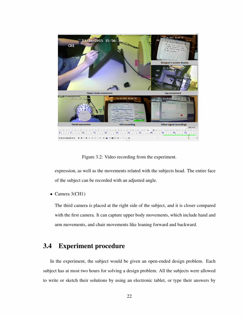
Figure 3.2: Video recording from the experiment.

expression, as well as the movements related with the subjects head. The entire face

of the subject can be recorded with an adjusted angle.

• Camera 3(CH1)

The third camera is placed at the right side of the subject, and it is closer compared

with the first camera. It can capture upper body movements, which include hand and

arm movements, and chair movements like leaning forward and backward.

3.4 Experiment procedure

In the experiment, the subject would be given an open-ended design problem. Each

subject has at most two hours for solving a design problem. All the subjects were allowed

to write or sketch their solutions by using an electronic tablet, or type their answers by

22

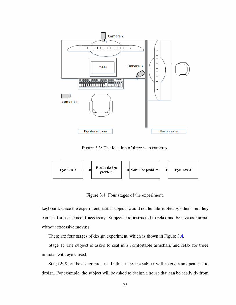
Figure 3.3: The location of three web cameras.

Figure 3.4: Four stages of the experiment.

keyboard. Once the experiment starts, subjects would not be interrupted by others, but they

can ask for assistance if necessary. Subjects are instructed to relax and behave as normal

without excessive moving.

There are four stages of design experiment, which is shown in Figure 3.4.

Stage 1: The subject is asked to seat in a comfortable armchair, and relax for three

minutes with eye closed.

Stage 2: Start the design process. In this stage, the subject will be given an open task to

design. For example, the subject will be asked to design a house that can be easily fly from

23

one place to another place.

Stage 3: After reading the information of the given problem, the subject is required to

write or draw answers by using the tablet. This session is continued for a maximum period

of 120 min with video monitoring. The subject is instructed to relax and behave as normal

without excessive moving. Only the minimal talking is permitted.

Stage 4: After the subject completes the design problem, the subject is asked to relax

for three minutes with eye closed.

The personal information of subjects and the number of segments are presented in Table

3.1.

Table 3.1: Number of segments for each subject.

Subject Gender Duration Number Total DesignID of segments seconds problem1 Male 0:14:01.216 6 18 Backpack2 Female 1:07:36.044 18 66 House3 Male 0:59:34.342 30 121 House4 Male 0:33:05.098 7 21 House5 Female 0:41:49.51 5 45 house6 Male 1:40:56.346 22 100 Shoes7 Male 0:17:36.39 4 11 House8 Female 0:51:24.548 19 49 House

3.5 Data pre-processing

The raw EEG data is collected during the completion of the experiment, and each

recording contains 64 EEG channels. The central electrode Cz was used as a common

reference. Moreover, these required bio-electrical signals are sampled with a frequency of

500 Hz.

In the pre-processing unit, filtering as a simple and traditional treatment is adopted

24

for the raw EEG data. As described in Chapter 2.2, the non-neural artifacts usually arise

from outside of the body, such as equipment and environment. In the experimental setup,

an uncontrolled variation exists due to the experimental error. It is nearly impossible to

completely eliminate this type of noise. While the environmental induced noises surround

the human body in daily living, such as mains power leads and white noise, can be prop-

erly filtered in frequency domain by using a band-pass filter. Filtering the unwanted com-

ponents will help to eliminate the majority of noises and improve signal-to-noise ratio

(K. T. Sweeney, Ward, & McLoone, 2012).

In this research, to eliminate the environment noises and keep maximum information

from the raw EEG data at the same time, the EEG signals were passed through a pre-defined

band-pass filter, and the setting of filter is from 0.3 Hz (forward, 6 dB/oct) to 70 Hz (zero

phase, 24 dB/oct). All the above preprocessing procedure has been performed in BESA

software.

25

Chapter 4

Movement-triggered Artifact Analysis

The entire procedure for movement-triggered artifact analysis can be divided into four

processing steps: preprocessing, segmentation, feature extraction/selection and compari-

son, as shown in Figure 4.1.

Following the pre-processing stage as described in Chapter 3, the next step is segmen-

tation. Since the original data contains a large amount of information, and processing the

whole dataset is difficult, a time period of interest needs to be selected for artifact analysis.

According to the video recording of the cognitive experiment process, the segments could

be created by setting boundaries at time instants corresponding to the changes of body

movements. With the help of a guideline predefined for segmentation, the contaminated

periods are identified by marking the exact beginning and end time of the movements.

In the next step, these extracted signals would be transformed in to a set of features

as reduced representation. From the previous studies, researchers analyze the EEG signals

based on their features to differentiate between normal and abnormal EEG signals. Thus,

the second block in this chapter named feature extraction is performed. To facilitate the

interpretation of EEG signals, the characteristics of the signals is supposed to be detected

and quantified through this section. The selection of features is based on the application.

In this situation, the power in the beta band may be relevant to muscle artifact.

26

Figure 4.1: The overview of movement-triggered artifact analysis.

During artifact analysis section, we mainly present a guideline to segment the raw EEG

signals. After that, the calculation of several parameters are presented for feature extraction.

In this way, EEG on the basis of its features in frequency domain is investigated.

4.1 EEG data segmentation

In the visual inspection of segmentation process, one observer is involved to mark the

movement-triggered segment accurately, who processes the same data twice to make sure

the beginning and the end of marking is reliable. All the video recording were displayed

in a computer software named Playback, and the EEG recording is performed in PyCorder

software showing all the channels page-by-page, each lasting 10 seconds.

27

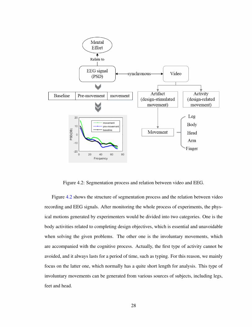
Figure 4.2: Segmentation process and relation between video and EEG.

Figure 4.2 shows the structure of segmentation process and the relation between video

recording and EEG signals. After monitoring the whole process of experiments, the phys-

ical motions generated by experimenters would be divided into two categories. One is the

body activities related to completing design objectives, which is essential and unavoidable

when solving the given problems. The other one is the involuntary movements, which

are accompanied with the cognitive process. Actually, the first type of activity cannot be

avoided, and it always lasts for a period of time, such as typing. For this reason, we mainly

focus on the latter one, which normally has a quite short length for analysis. This type of

involuntary movements can be generated from various sources of subjects, including legs,

feet and head.

28

To extract the segments of movement-triggered EEG signals, we define a set of criteria

as following:

• Subjects should be in any stage of design process as defined in Chapter 3. There

should be a minimum of ten continuous seconds before a movement-triggered signal

could be segmented.

• The movement generated by the subject should have a duration of at least 2 seconds

or greater to be marked as movement-triggered EEG signals.

• A minimum of ten continuous seconds of interval is required to segment a second

movement-triggered epoch.

• The occurrence of movements should be considered only if the movement is sig-

nificant in the video and unrelated with output of the design process. As we dis-

cussed in section 2.2.3, where we define the movements for analysis, several typical

movements would be recorded, including leg movement, head movement and body

movement.

In general, this segmentation guideline is not a strictly defined procedure, and it also

allows subjectivity in capturing movement artifacts. In this research, we use large-scale

physical movements which can be identified by the video recording. The start time and end

time are recorded in the time table along with a brief behavior description. Table 4.1 shows

part of the time table of body movements, which is used to extract movement-triggered

segments for further analysis.

After marking the segments when movements occur, we extract two more segments

as well, in order to investigate the transition from non-movement state to movement one.

When we compare the differences of these two states, inter-subject variability is supposed

to be reduced by using reference. Therefore, we define three types of segments for inves-

tigating the impact of body movement on EEG signals. Figure 4.3 illustrates how these

29

Table 4.1: Time table of physical movements for segmentation

Movement EEG recording Duration DescriptionNo. Start time End time (seconds) of movements1 0:07:44 0:07:50 6 move body2 0:09:16 0:09:21 5 move body3 0:10:04 0:10:08 4 move body4 0:11:55 0:11:58 3 move leg5 0:12:51 0:12:56 5 move leg, body slightly6 0:13:35 0:13:38 3 move body7 0:19:34 0:19:36 2 move leg (a little)8 0:20:59 0:21:02 3 move body (swivel in the

chair)9 0:22:35 0:22:37 2 move body (swivel in the

chair)10 0:25:59 0:26:02 3 move leg, then move body by

swiveling the chair11 0:26:32 0:26:37 5 move body (swivel in the



chair)14 0:39:47 0:39:49 2 move leg (a little)15 0:53:29 0:53:31 2 move body (swivel in the

chair) slightly16 1:00:29 1:00:38 9 move body (swivel in the

chair) largely, move leg17 1:03:15 1:03:20 5 move body (swivel in the

chair) slightly18 1:04:35 1:04:38 3 move leg

30

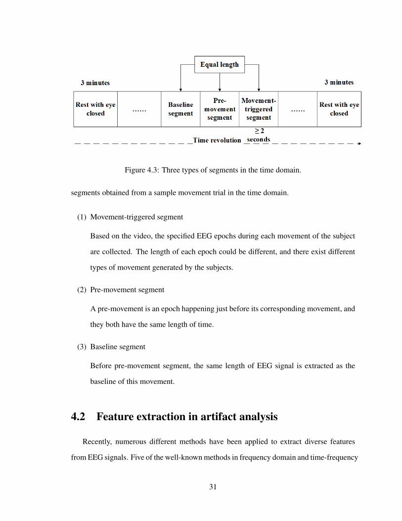
Figure 4.3: Three types of segments in the time domain.

segments obtained from a sample movement trial in the time domain.

(1) Movement-triggered segment

Based on the video, the specified EEG epochs during each movement of the subject

are collected. The length of each epoch could be different, and there exist different

types of movement generated by the subjects.

(2) Pre-movement segment

A pre-movement is an epoch happening just before its corresponding movement, and

they both have the same length of time.

(3) Baseline segment

Before pre-movement segment, the same length of EEG signal is extracted as the

baseline of this movement.

4.2 Feature extraction in artifact analysis

Recently, numerous different methods have been applied to extract diverse features

from EEG signals. Five of the well-known methods in frequency domain and time-frequency

31

domain have been discussed (Al-Fahoum & Al-Fraihat, 2014), which are time frequency

distributions (TFD), fast Fourier transform (FFT), eigenvector methods (EM), wavelet trans-

form (WT) and auto-regressive method (ARM). After comparing their performances, it is

indicated that there does not exist an optimum method for all applications.

To increase the computational efficiency and get some basic information in artifact

analysis, we narrow down the number of channels in the first step. According to the 64-Ch

standard electrode layout for actiCHamp, the six channels C3, C4, P3, P4, P7, P8 which are

usually used for detecting muscle artifact are selected for data comparison (Van de Velde,

van Erp, & Cluitmans, 1998). For each channel, the absolute power of different frequency

bands can be obtained in each type of segment. After that, the same procedure will be

repeated for all other 57 channels except the reference channel Cz for statistical analysis.

4.2.1 Power spectral analysis

In frequency domain, the power spectral density is a widely-used method to describe

the power intensity of the signal. Power spectral analysis transforms a signal from time

domain to frequency domain, and characterizes the relationship between amplitude and

frequency. Almost all the available spectral analysis techniques are based on the Fourier

transform, whose inverse also allows the signal to be recovered from the transformed one.

The discrete Fourier transform (DFT) decomposes a signal into its frequency components,

as expressed by Eq. (1):

DFTx(n) = X(k) =N−1∑n=0

x(n)e(−j2πNnk)(0 ≤ k ≤ N − 1) (1)

The inverse discrete Fourier transform is given by Eq. (2):

IDFT{x(k)} = X(n) =1

N

N−1∑k=0

X(k)e(j2πNnk)(0 ≤ n ≤ N − 1) (2)

32

In practice, the Fast Fourier transform (FFT) is oftern used for fast computation of the

DFT. When the data is deterministic with no random effects, a Fourier transform is directly

performed to decompose the signal into a sum of sinusoids of difference frequencies. How-

ever, the real signal is always obscured by unwanted noise. To obtain the desired features

while suppressing the noise, the PSD estimation is often calculated through efficient meth-

ods, such as averaging or smoothing. In general, there are two main methods for power

spectral density estimation, non-parametric and parametric.

Parametric methods typically set signal models with assumption to calculate power

spectral density estimate. Based on linear prediction, the autoregressive (AR) method is

frequently used in practice for the ease of computing PSD through AR coefficients. The

autoregressive method performs well in moderate-to-high SNR ranges, for narrowband

signals, the performance of this method highly depends on the model order selector. If

the model order is too small, the spectrum will lack resolution and have a highly smoothed

effect. If the order selected is too high, false peaks would then occur.

For a wide-sense stationary process, the power spectral density cannot be consistently

estimated from periodogram. Therefore, Welchs technique (Welch, 1967) is introduced as

a non-parametric method to estimate PSD. To reduce the variance of the periodogram, this

method breaks the time series into segments, each segment being multiplied by a window

function, such as Hamming window. Then, a modified periodogram is computed for each

segment, and all the resulting periodograms from different segments are averaged to es-

timate the power spectral density. The segments usually overlap to avoid the information

loss caused by windowing (Solomon Jr, 1991). This method is briefly explained as follows.

We assume x(0), x(1), · · · , x(N − 1) as a signal in time domain, and partition the data

sequence in to K segments of length M. The k-th segment can be denoted as xk(i), i =

S, · · · ,M + S − 1 where S is the shift points between segments. The windowed discrete

33

Fourier transform (DFT) is computed as:

Xk(f) =∑m

xk(m)W (m)e(−2πj)(mf) (3)

where m = S(k − 1), · · · ,M + S(k − 1) and W(m) is the window function.

The modified periodogram for each segment Pk(f) is then calculated as:

Pk(f) =1

W|Xk(f)|2

W =M∑m=0

[W (m)]2(4)

At last, we obtain Welchs estimate of PSD by averaging the periodogram values:

PSD(f) =1

K

K∑k=1

Pk(f) (5)

In this thesis, Welchs method is applied to estimate the power spectra with a Ham-

ming window of 1-second duration with 50% overlap since EEG signal is non-stationary.

Figure 4.4 shows the PSD of one channel, computed for movement-triggered segment,

pre-movement segment and baseline segment.

In order to distinguish the movement-triggered segments and no-movement segments,

several parameters in the frequency domain are chosen:

(1) Total power in 4-30 Hz

In this thesis, the total power is defined as the band power in frequency interval of 4

to 30 Hz. The frequency below 4 Hz is not included in the calculation of total power.

(2) Relative power in Beta2 band

The relative power is defined as the percentage of the total power in this specified fre-

quency interval. It is reported that Beta activity mostly occurs during active thinking.

34

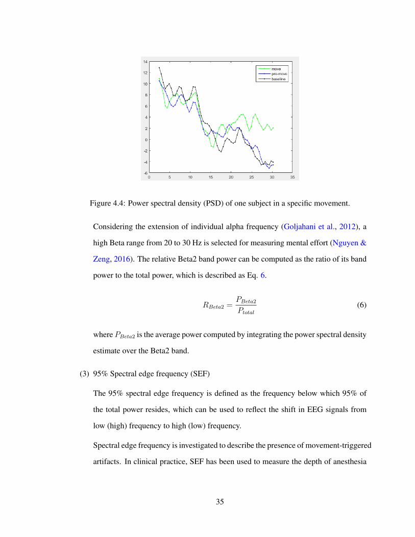
Figure 4.4: Power spectral density (PSD) of one subject in a specific movement.

Considering the extension of individual alpha frequency (Goljahani et al., 2012), a

high Beta range from 20 to 30 Hz is selected for measuring mental effort (Nguyen &

Zeng, 2016). The relative Beta2 band power can be computed as the ratio of its band

power to the total power, which is described as Eq. 6.

RBeta2 =PBeta2Ptotal

(6)

where PBeta2 is the average power computed by integrating the power spectral density

estimate over the Beta2 band.

(3) 95% Spectral edge frequency (SEF)

The 95% spectral edge frequency is defined as the frequency below which 95% of

the total power resides, which can be used to reflect the shift in EEG signals from

low (high) frequency to high (low) frequency.

Spectral edge frequency is investigated to describe the presence of movement-triggered

artifacts. In clinical practice, SEF has been used to measure the depth of anesthesia

35

and indicate intra-operative movements (Schwender et al., 1996). Besides, as a fre-

quency domain parameter, SEF is applied to detect short periods muscle artifacts

automatically in normal awake EEG signals (Van de Velde et al., 1998).

4.2.2 Wavelet analysis

Based on the uncertainty principle, when the window size gets narrow, the frequency

solution becomes poor, and vice versa. As the signals we applied are localized with quite

short length in time series, similar with ERP components, their power spectral analysis

based on short-time Fourier transform has limited performance. For this reason, wavelet

is proposed as an effective technique dealing with transient signals, which exploits the in-

formation from both time and frequency domains. Also, there is no assumption for the

stationarity of the recorded signals. Moreover, wavelet transform can be used in many

domains of bio-signal processing, such as the seizure epileptic diagnosis (Adeli, Zhou, &

Dadmehr, 2003) (Guo, Rivero, Seoane, & Pazos, 2009) (Kumar, Dewal, & Anand, 2012)

and the classification of movement-related cortical potentials (MRCPs) (Farina, do Nasci-

mento, Lucas, & Doncarli, 2007).

The wavelet transform decomposes a signal into a set of basic functions called wavelets.

A signal in general can be considered as a superposition of different structures occurring

on different time scales at different times or spatial scales at different locations. A set

of elementary functions can be applied as mother wavelets for decomposition of original

signals. Examples of traditional wavelets are Haar and Daubechies wavelets. As the main

base of wavelet transform, the selection of mother wavelet function will affect the precision

for identifying the desired signals.

In general, two types of wavelet analysis exist in data processing, namely continuous

wavelet transform (CWT) and discrete wavelet transform (DWT). The continuous wavelet

36

transform (CWT) of a signal x(t) is defined as Eq.7:

CWT (a, b) =

∫ ∞−∞

1√|a|x(t)Ψ(

t− ba

)dt (7)

where a and b are the scale and shifting parameters, respectively. The wavelet becomes

narrower when the value of a increases.

When a = 2j and b = 2jk, we have

CWT (a, b) =

∫ ∞−∞

1√|2j|

x(t)Ψ(t− 2jk

2j)dt (8)

According to Nyquist rule, the raw signal is down-sampled by two and the output signal

has maximum one-half of the frequency bandwidth.

Multi-resolution representation provides an effective way of implementing DWT (Mal-

lat, 1989). This decomposition is computed with a pyramidal algorithm based on convo-

lutions by quadrature mirror filters, which contain a series of high-pass (HP) and low-pass

(LP) filter pairs. In DWT filter implementation, the output signal of high-pass filter corre-

sponds to the detailed wavelet coefficients, and low-pass filter produces the approximation

coefficients of each level. The whole process of decomposition is illustrated in Figure 4.5.

The frequency bands of signal component Dj(k) and Aj(k) can be obtained as:

Dj(k) : [fs

2j+1,fs2j

]

Aj(k) : [0,fs

2j+1]

(9)

where j = 1, 2, · · · , J

The approximation and detailed coefficients could provide information of the signal in

different frequency bands. Each band is defined according to the level of decomposition

and the sample rate of the original EEG signals.

37

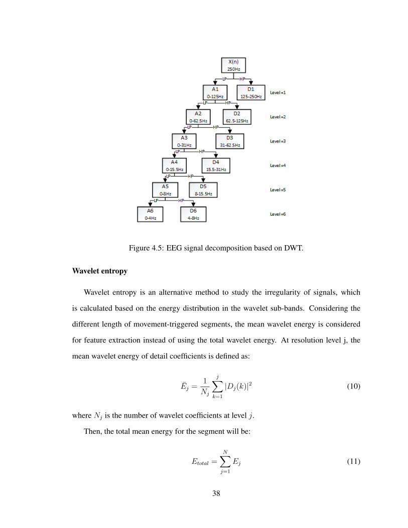
Figure 4.5: EEG signal decomposition based on DWT.

Wavelet entropy

Wavelet entropy is an alternative method to study the irregularity of signals, which

is calculated based on the energy distribution in the wavelet sub-bands. Considering the

different length of movement-triggered segments, the mean wavelet energy is considered

for feature extraction instead of using the total wavelet energy. At resolution level j, the

mean wavelet energy of detail coefficients is defined as:

Ej =1

Nj

j∑k=1

|Dj(k)|2 (10)

where Nj is the number of wavelet coefficients at level j.

Then, the total mean energy for the segment will be:

Etotal =N∑j=1

Ej (11)

38

The relative wavelet energy in time evolution is calculated by:

pj =EjEtotal

(12)

The wavelet entropy for each channel r can be obtained by:

WEr = −N∑j=1

pj ln (pj) (13)

The wavelet transform-based entropy not only measures the degree of order (disor-

der) of signal segments, but also reflects the underlying dynamical process in consequence

(Rosso, Blanco, & Figliola, 2004).

Relative wavelet entropy

As described before, the wavelet entropy of each segment can be calculated straightfor-

wardly. To measure the degree of similarity between two segments on the other hand, the

so-called relative wavelet entropy was introduced in (Rosso et al., 2001) as well.

The probability distribution of the wavelet energy for two EEG segments could be rep-

resented as {pj} and{qj}, with∑

j pj =∑

j qj = 1. The relative wavelet entropy is then

calculated as

RWT (p|q) =N∑j=1

pj ln (pjqj

) (14)

where the distribution {qj} is taken as a reference distribution. If pj ≡ qj , the RWE

vanishes.

39

4.3 Experimental results

EEG recording is a mixture of underlying brain potentials and additional waveforms.

Considering the main purpose of this research, the actual signal of interest is movement-

triggered artifact during cognitive tasks. In most circumstances, this type of artifacts are

identified from raw data after the contaminated channels or epochs are rejected through

visual inspection, and characterized for further detection and removal. In recent studies,

some efforts have also been made to separate artifacts from scalp EEG. For example, a

non-conductive layer (a silicone swim cap) is placed over the scalp of subjects, in order to

block electro-physiological signals from electrodes, and thus directly record the movement

artifact signals during walking (Kline, Huang, Snyder, & Ferris, 2015). During design ac-

tivities, however, the movements generated by subjects are unpredictable in advance and

hardly repeatable, and therefore we cannot isolate and record the movement-triggered ar-

tifact for further analysis. For this consideration, we examine the following two types of

consecutive periods from raw data to perform the variability tracking, named as test period

and context period, respectively. In the test period, the statistical significance is examined

by comparing the variances of movement-triggered and pre-movement segments. In the

context period, the variances of pre-movement and baseline segments are compared for

statistical analysis.

A graphical user interface (GUI) is developed in Matlab to analyze EEG signals from

eight subjects, as shown in Figure 4.6. Figure 4.7 indicates the power spectral density of

movement 5 (Subject 3) in frontal lobe.

4.3.1 Results using relative Beta2 power

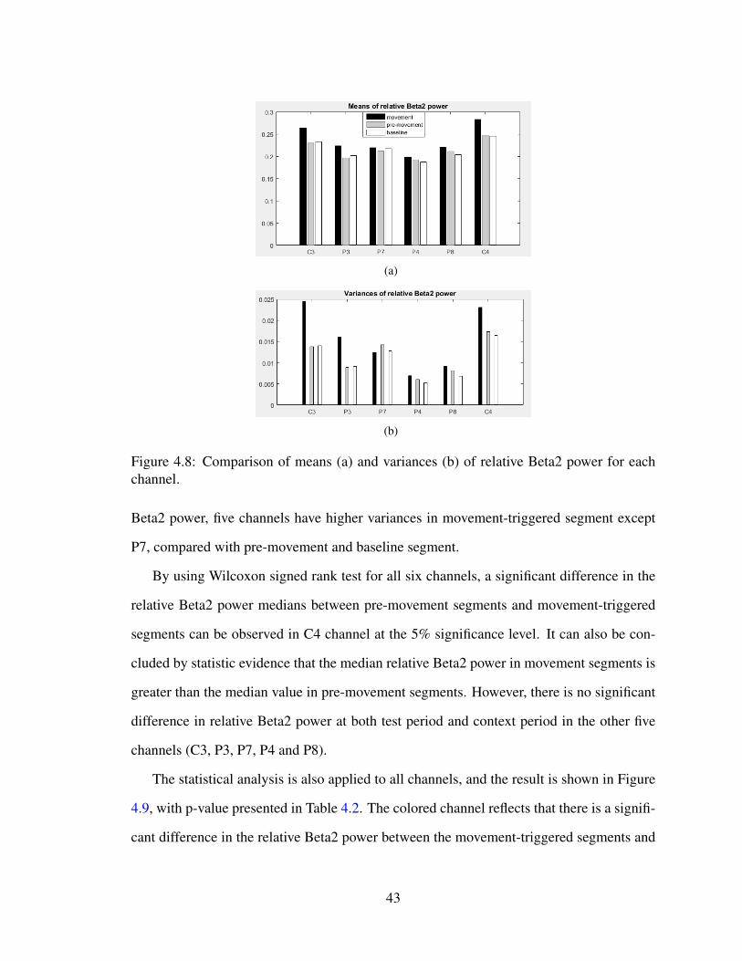
Figure 4.8 shows that the average relative Beta2 power for six channels in three types

of segments. For all subjects, it can be observed the mean value in movement-triggered

segment is always greater than the other two types of segments. For the variance of relative

40

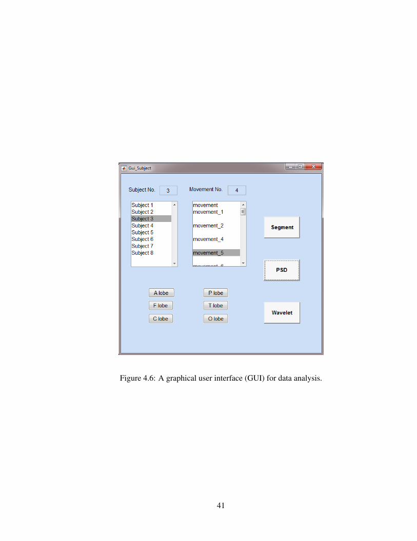
Figure 4.6: A graphical user interface (GUI) for data analysis.

41

Figu

re4.

7:A

nex

ampl

eof

PSD

ingr

aphi

calu

seri

nter

face

(GU

I).

42

(a)

(b)

Figure 4.8: Comparison of means (a) and variances (b) of relative Beta2 power for eachchannel.

Beta2 power, five channels have higher variances in movement-triggered segment except

P7, compared with pre-movement and baseline segment.

By using Wilcoxon signed rank test for all six channels, a significant difference in the

relative Beta2 power medians between pre-movement segments and movement-triggered

segments can be observed in C4 channel at the 5% significance level. It can also be con-

cluded by statistic evidence that the median relative Beta2 power in movement segments is

greater than the median value in pre-movement segments. However, there is no significant

difference in relative Beta2 power at both test period and context period in the other five

channels (C3, P3, P7, P4 and P8).

The statistical analysis is also applied to all channels, and the result is shown in Figure

4.9, with p-value presented in Table 4.2. The colored channel reflects that there is a signifi-

cant difference in the relative Beta2 power between the movement-triggered segments and

43

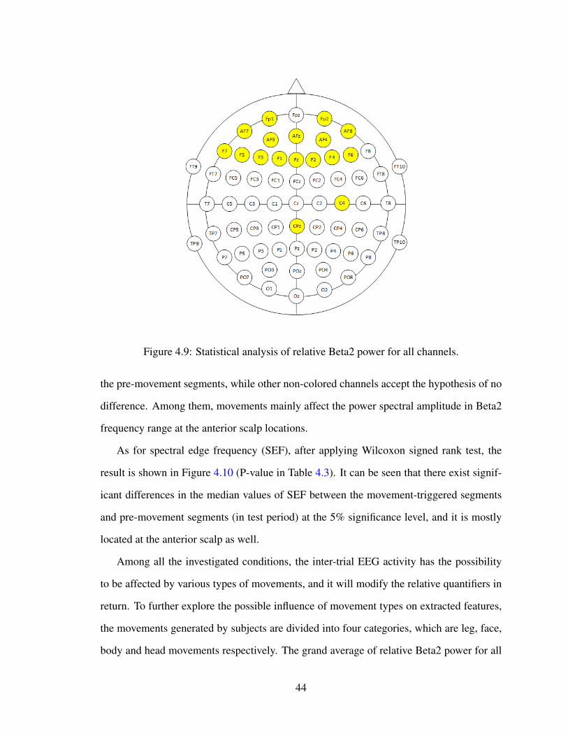
Figure 4.9: Statistical analysis of relative Beta2 power for all channels.

the pre-movement segments, while other non-colored channels accept the hypothesis of no

difference. Among them, movements mainly affect the power spectral amplitude in Beta2

frequency range at the anterior scalp locations.

As for spectral edge frequency (SEF), after applying Wilcoxon signed rank test, the

result is shown in Figure 4.10 (P-value in Table 4.3). It can be seen that there exist signif-

icant differences in the median values of SEF between the movement-triggered segments

and pre-movement segments (in test period) at the 5% significance level, and it is mostly

located at the anterior scalp as well.

Among all the investigated conditions, the inter-trial EEG activity has the possibility

to be affected by various types of movements, and it will modify the relative quantifiers in

return. To further explore the possible influence of movement types on extracted features,

the movements generated by subjects are divided into four categories, which are leg, face,

body and head movements respectively. The grand average of relative Beta2 power for all

44

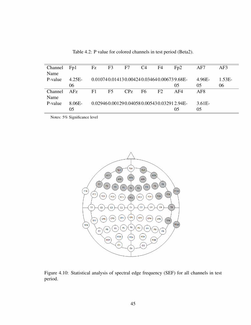
Table 4.2: P value for colored channels in test period (Beta2).

ChannelName

Fp1 Fz F3 F7 C4 F4 Fp2 AF7 AF3

P-value 4.25E-06

0.010740.014130.004240.034640.006739.68E-05

4.96E-05

1.53E-06

ChannelName

AFz F1 F5 CPz F6 F2 AF4 AF8

P-value 8.06E-05

0.029460.001290.040580.005430.032912.94E-05

3.61E-05

Notes: 5% Significance level

Figure 4.10: Statistical analysis of spectral edge frequency (SEF) for all channels in testperiod.

45

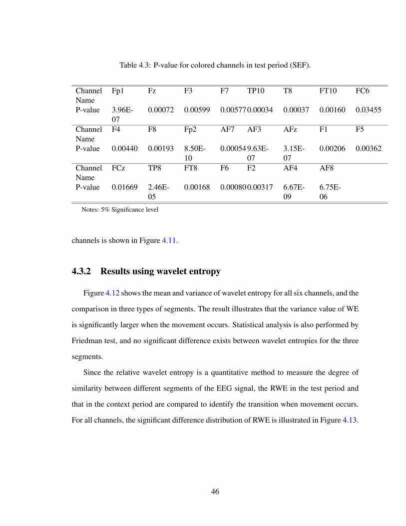
Table 4.3: P-value for colored channels in test period (SEF).

ChannelName

Fp1 Fz F3 F7 TP10 T8 FT10 FC6

P-value 3.96E-07

0.00072 0.00599 0.005770.00034 0.00037 0.00160 0.03455

ChannelName

F4 F8 Fp2 AF7 AF3 AFz F1 F5

P-value 0.00440 0.00193 8.50E-10

0.000549.63E-07

3.15E-07

0.00206 0.00362

ChannelName

FCz TP8 FT8 F6 F2 AF4 AF8

P-value 0.01669 2.46E-05

0.00168 0.000800.00317 6.67E-09

6.75E-06


channels is shown in Figure 4.11.

4.3.2 Results using wavelet entropy

Figure 4.12 shows the mean and variance of wavelet entropy for all six channels, and the

comparison in three types of segments. The result illustrates that the variance value of WE

is significantly larger when the movement occurs. Statistical analysis is also performed by

Friedman test, and no significant difference exists between wavelet entropies for the three

segments.

Since the relative wavelet entropy is a quantitative method to measure the degree of

similarity between different segments of the EEG signal, the RWE in the test period and

that in the context period are compared to identify the transition when movement occurs.

For all channels, the significant difference distribution of RWE is illustrated in Figure 4.13.

46

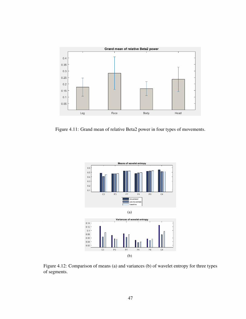
Figure 4.11: Grand mean of relative Beta2 power in four types of movements.

(a)

(b)

Figure 4.12: Comparison of means (a) and variances (b) of wavelet entropy for three typesof segments.

47

Figure 4.13: Statistical analysis of relative wavelet entropy (RWE) for all channels.

Table 4.4: P value for colored channels in test period (RWE).

ChannelName

Fp1 Fz Pz O1 Oz TP10 CP6 T8 FT10 Fp2

P-value 0.008310.025540.004240.004820.011785.91E-05

0.041160.000400.006550.03592

ChannelName

AFz PO7 PO3 POz CPz TP8 FT8 F2 AF4

P-value 0.046060.014840.027330.016220.011110.02946 0.022940.036440.04145


48

Chapter 5

Artifact Removal

Actually, it is nearly impossible to avoid the occurrence of ocular and muscle activity

in monitoring brain signals. In clinical practice, the most direct approach is the rejection of

entire contaminated data segments. Based on the expertise of experts, the trials are checked

visually and removed from the analysis. This method mostly relies on human experts or

well-trained experimenters who can identify all types of artifact epochs from the original

recording, so as to make sure the data applied in analyses represent real brain activity.

However, there exist many disadvantages with rejection of contaminated EEG segments.

The first one is that the selection of artifact may be subjective, thus, it is usually affected

by the expert performance. At the same time, it is a time consuming task, especially for

a large amount of recorded data. Moreover, the biggest problem of manual rejection is a

substantial information loss, which could cause a huge drawback on the analysis section

and consequently reduce the quality of desired data. To overcome these drawbacks, several

automatic artifact removal approaches have been proposed in recent studies.

The raw signal recorded from the experiment is X(n), which is a combination of the

underlying brain activity R(n) and the unwanted noise N(n), as illustrated in Figure 5.1. The

function f describes how the artifact modifies the desired signal, which contains additive

or multiplicative artifacts. While additive artifact is predominantly considered because it

49

Figure 5.1: General framework of signal combination.

is easy to handle in practice. Also, the majority of artifact removal techniques assume that

the number of sources should be equal or smaller than the recorded channels, especially for

blind source separation techniques.

In this chapter, two commonly used algorithms are reviewed for artifact removal, namely,

canonical correlation analysis (CCA) and independent component analysis (ICA). The ex-

perimental procedure of movement-triggered artifact removal is shown in Figure 5.2.

5.1 Canonical correlation analysis (CCA)

In blind source separation by canonical correlation analysis (BSS-CCA) for artifact re-

moval, the contaminated EEG signal is generated by both brain source and muscle activity.

It assumes these sources are uncorrelated and maximally auto-correlated. Compared with

brain activity, muscle artifact always has relative low autocorrelation. Therefore, BSS-CCA

can separate the muscle and brain activity sources and remove the movement-triggered ar-

tifact (Clercq et al., 2006).

Let X(t) be the raw data in time domain, which is represented as:

X(t) = [x1(t), x2(t), · · · , xR(t)]T (t = 1, · · · , N) (15)

with N being the number of sample points and R the number of channels. We assume the

50

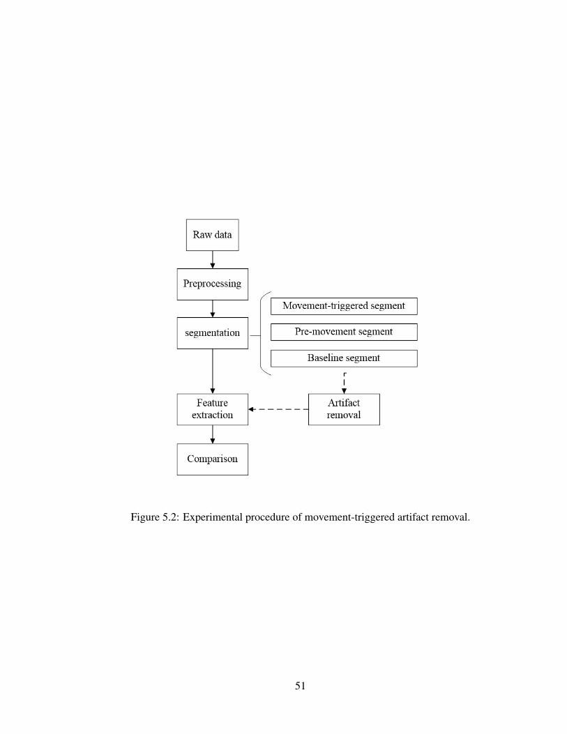
Figure 5.2: Experimental procedure of movement-triggered artifact removal.

51

EEG raw signal recorded from the experiment is an unknown mixture of a set of source

signals S(t) = [s1(t), s2(t), · · · , sR(t)]T , with equality number of sources and channels,

and linear mixing. The raw data can be obtained by a matrix multiplication:

X(t) = MS(t) (16)

where M is an unknown mixing matrix. To recover the source signals S(t), the mixing

matrix should be estimated beforehand. It can be obtained by introducing de-mixing matrix

A as:

S(t) = AX(t) (17)

Normally, A is the inverse of the mixing matrix M from the previous equation.

Let Y (t) be a temporal delayed matrix of the raw data X(t) with one sample lag, repre-

sented as Y (t) = X(t− 1). Considering the linear combination of the source components

forX(t) and Y (t), the variates are defined as:

u = ax1x1 + · · ·+ axRxR = aTxX

v = ay1y1 + · · ·+ ayRyR = aTy Y

(18)

where ax = [ax1 , · · · , axR ]T and ay = [ay1 , · · · , ayR ]T are the weight vectors.

Since the sources are supposed to be maximally auto-correlated, the correlation ρ be-

tween u and v also need to be maximized as below to meet the assumption:

maxax,ay

ρ(u, v) =E[uv]√E[u2]E[v2]

=aTxCxyay√

(aTxCxxax)(aTyCyyay)

(19)

where Cxx and Cyy are the autocovariance matrix of X and that of Y , respectively, and Cxy

52

is the cross-covariance matrix of X and Y . After some manipulations, we obtain

{Cxx−1CxyCyy−1Cyxax = ρ2ax

Cyy−1CyxC

−1xx Cxyay = ρ2ay

(20)

The square root of the eigenvalue is the canonical correlation coefficient ρ, and the

eigenvectors are ax and ay. Actually, X and Y contain almost the same data, so the same

data is also contained in ax and ay. Therefore, solving ax is sufficient. The first variates are

constructed and the relation between u1(t) and v1(t) is:

v1(t) = aTy Y (t) = aTxX(t− 1) = u1(t− 1) (21)

Consequently, the transformation given by ax produces the source u1(t), which has

the maximal autocorrelation. The next variates yield ui(t) that has maximal autocorrela-

tion among all possible linear combination, but they are uncorrelated with the previously

ui−1(t). The sources are obtained as Si(t) = ui(t). These source signals are uncorrelated

with each other, but maximally auto-correlated and in a decrease of autocorrelation index

order.

The aim of this section is to remove muscle artifact by using canonical correlation

analysis (CCA). According to the visual inspection by experienced experts, the movement-

triggered segments are obtained, which contain not only muscle activity but also the activity

from the brain. When applying BSS-CCA in the extracted movement-triggered segment,

the muscle artifact is supposed to be removed through setting artefactual sources equal to

zero. For the reconstructed segment

Xdenoised(t) = MS(t) (22)

withM being the mixing matrix with the zero value of muscle artifact sources, and S(t) the

53

sources calculated by BSSCCA. The investigation in (Goncharova et al., 2003)has identi-

fied the common noise-like pattern of EMG contamination that comprises irregular spikes.

Thus, a low autocorrelation is expected for muscle artifact, and we assume it is present in

the lowest auto-correlated BSSCCA source.

The pre-movement segment is selected as underlying brain signal for comparison, and

in the selected EEG signals, we assume that no muscle artifact exists.

5.2 Independent component analysis (ICA)

In the beginning, Independent component analysis (ICA) was proposed for separating

source signals from the mixtures by statistical properties, which is widely known as the

cocktail-party problem (Hyvrinen & Oja, 2000). With the increasing interest of ICA, there

are a variety of practical real-life applications which includes for example biomedical sig-

nal analysis and processing. As for EEG signal, it measures the electrical potentials in

different locations over the scalp. The brain activity can be regarded as a mixture of the

underlying components. Based on the assumption that the source components are statisti-

cally independent, the source signals of the brain can be separated from the mixture EEG

potentials.

In the ICA model, assuming that we obtain the raw EEG data X(t) in time domain,

which is represented as X(t) = [x1(t), x2(t), · · · , xR(t)]T (t = 1, · · · , N), with N being

the number of sample points and R the number of channels. While the underlying indepen-

dent components are represented by S(t) = [s1(t), s2(t), · · · , sR(t)]T . The mixing model

can be written as:

X(t) = MS(t) (23)

where M is the mixing matrix. The independent components and the mixing matrix cannot

54

be observed directly, however, both of them are estimated from the mixture X(t) with gen-

eral assumptions. Apart from the assumption of spatial statistical independence of sources,

we also assume that the independent component should follow non-Gaussian distribution.

Moreover, the unknown mixing matrix is always assumed to be square. After obtaining the

matrix M , its inverse, which is represented as A, can be used to compute the independent

component by:

S(t) = AX(t) (24)

For artifact removal, EEG data recorded from the scalp can be considered as summa-

tions of EEG data and artifact, and the contaminating noise can be assumed to be indepen-

dent of the underlying brain sources. Based on ICA which is also a blind source separation

(BSS) problem, this method transforms the input vector into a signal space in which the sig-

nals are statistically independent. After the transformation of the EEG signals, non-artifact

neural sources should be selected and reconstructed without the artefactual components.

The subjective and time-consuming selection of ICA components is a typical problem

for researchers. To reduce the user dependent factor, in this thesis, we have applied an au-

tomatic method named Multiple Artifact Rejection Algorithm (MARA) for classification

of general artefactual source components. This method is proposed in (Winkler, Haufe,

& Tangermann, 2011) and it proves to be an efficient and reliable to detect all classes of

artifacts, such as eye and muscle artifacts. Based on six constructed features, MARA in-

corporates the information from temporal, spectral and spatial domain of the components.

This classifier was trained by brain experts based on a large amount of data. It provides an

open-source plug-in for a widely-used graphic user interface named EEGLAB (Delorme

& Makeig, 2004), in order to automatize the process of hand-labeling independent compo-

nents. Since ICA is sensitive to slow drifts, band-pass filtering the data can improve the

quality of the decomposition. The EEG data are filtered offline before segmentation and

artifact removal process, by using an FIR filter in advance. The power spectrum between 2

55

Hz and 39 Hz is recommended for feature calculation in MARA.

For an automatic classification method, substantial information need to be provided

in feature extraction process. Based on the characteristic of independent component, an

initial feature set with the collection of 38 features as candidates is constructed, which

contains 13 features derived from a component’s time series, 9 features from spectrum and

16 from component’s pattern. These six features were selected out of 38 features by a

feature selection procedure in (Winkler et al., 2011).

• Current density norm

The information of source locations cannot be provided by independent component

itself, however, it can be estimated by EEG potentials in ICA scalp map.

• Range within pattern

In a scaly map, the logarithm of the difference between the minimal and the max-

imal activation is calculated. A high range within pattern always indicates that the

spatially located scalp map is generated from muscle artifact or loose electrodes.

• Mean local skewness

This feature is derived from a components time series, and it is obtained by the mean

absolute local skewness of time intervals with a duration of 15s, with the purpose of

detecting outliers in time domain.

• λ and fit error

The deviation of one component’s spectrum from a 1/frequency curve and its shape

can be described by two features. For each component, the prototypical curve can

be shaped by six points of the log spectrum, including 1) the log power at 2 Hz, 2)

the log power at 3 Hz, 3) local minimum point in the band 5 -13 Hz, 4) the point 1

Hz below the third point, 5) local minimum point in the band 33-39 Hz, 6) the point

56

1Hz below the fifth point. The logarithm of λ and the mean squared error of the

approximation of f to the real spectrum in 8 to 15 Hz range are applied as features.

• 8-13 Hz

This feature indicates the average log band power of alpha band from 8 to 13 Hz,

with the purpose of detecting the alpha peak in the component of neural origin.

After the automatic classification of artefactual components by MARA, EEGLAB pro-

vides the interface to help the experimenters visualize all the independent components and

calibrate the components for rejection. Moreover, for each independent components, the

scalp map and spectrum are provided for visualization, as well as the probability of being

an artifact computed by MARA.

5.3 Expermental results

In this section, we define two consecutive EEG periods to perform the variability track-

ing, named as reconstructed period and context period, respectively. In reconstructed pe-

riod, the statistical significance is examined by comparing the parameter difference of re-

constructed segments and pre-movement segments. In context period, the parameter differ-

ence of pre-movement and baseline segments are compared for statistical analysis.

5.3.1 CCA

Relative Beta2 power

Wilcoxon signed rank test shows that there is no significant difference for all six chan-

nels between the reconstructed segment after CCA and pre-movement segment. Compared

with the result of original data, the difference changes in C4 channel.

57

(a)

(b)

Figure 5.3: Comparison of means (a) and variances (b) of relative Beta2 power for eachchannel after applying CCA.

Figure 5.3 gives the mean and variance comparison for all the six channels. As shown,

the mean value of the reconstructed segments decreases after applying CCA, and the same

trend exists in variance as well.

For all channels, the EEG signal is characterized with relative Beta2 power dominating

over anterior areas, as shown in Figure 5.4. Compared with the colored channels identified

in Figure 4.9 (Section 4.3.1), significant differences still exist in almost all these colored

channels except C4.

Spectral edge frequency (SEF)

After removing artifact by using BSS-CCA algorithm, the statistical differences in SEF

medians between pre-movement segments and movement-triggered segments (in test pe-

riod) are shown in Figure 5.5. This result suggests that there are more channels in central

area which change the power distribution in the frequency domain.

58

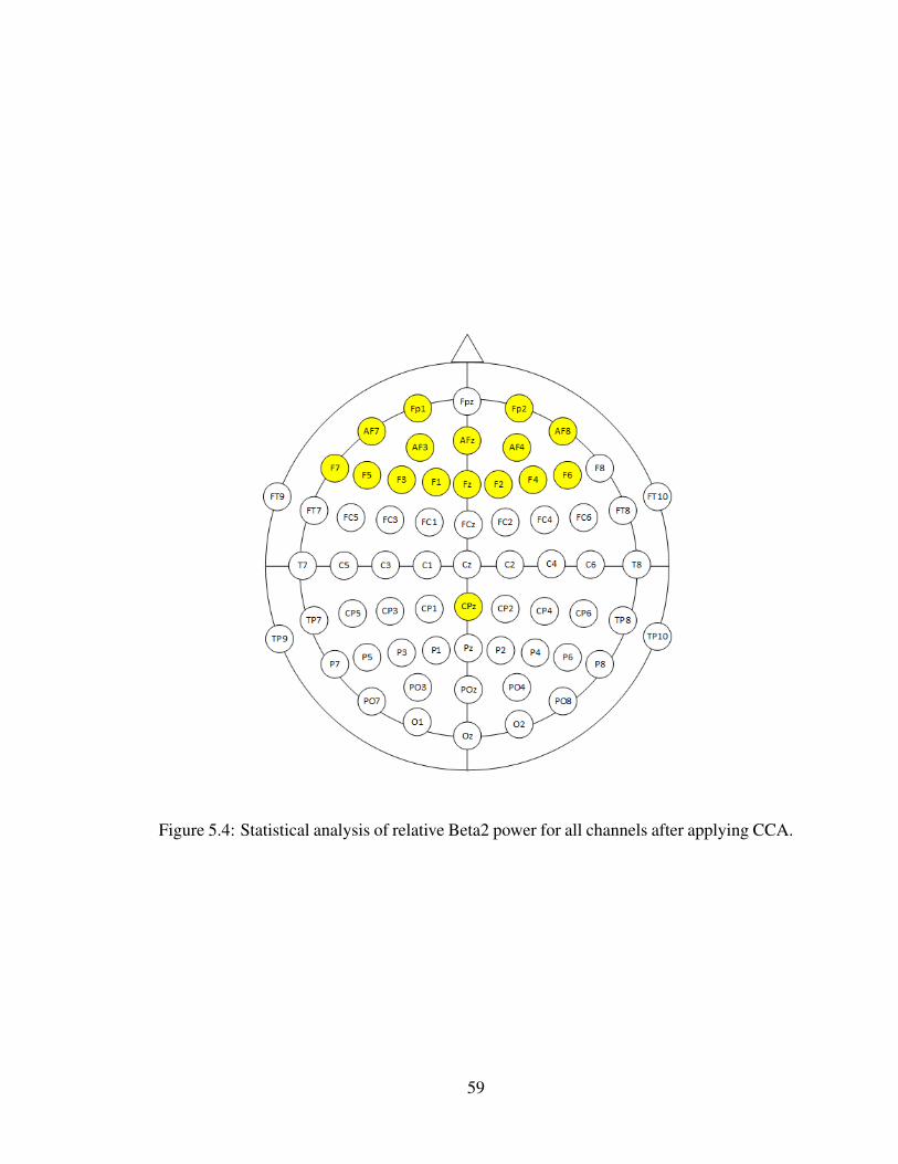
Figure 5.4: Statistical analysis of relative Beta2 power for all channels after applying CCA.

59

Figure 5.5: Statistical analysis of spectral edge frequency (SEF) for all channels in recon-structed period after applying CCA.

60

(a)

(b)

Figure 5.6: Comparison of means (a) and variances (b) of wavelet entropy for each channelafter applying CCA.

Wavelet entropy

Figure 5.6 shows the mean and variance of wavelet entropy for all six channels, and

the comparison in four types of segments. After applying CCA for movement-triggered

segments, both the mean and the variance values of WE reduce for all six channels. Statis-

tical analysis illustrates that no significant difference exists between wavelet entropies by

Friedman test.

For investigating the transition of wavelet entropy, statistical analysis is applied in rel-

ative wavelet entropy for all channels. Figure 5.7 presents the result of the relative wavelet

entropy difference when employed on the EEG data for all channels using CCA technique.

Compared with the result shown in Figure 4.13 (Section 4.3.2), the degree of similarity

between context period and test period changes in more channels after artifact removal.

61

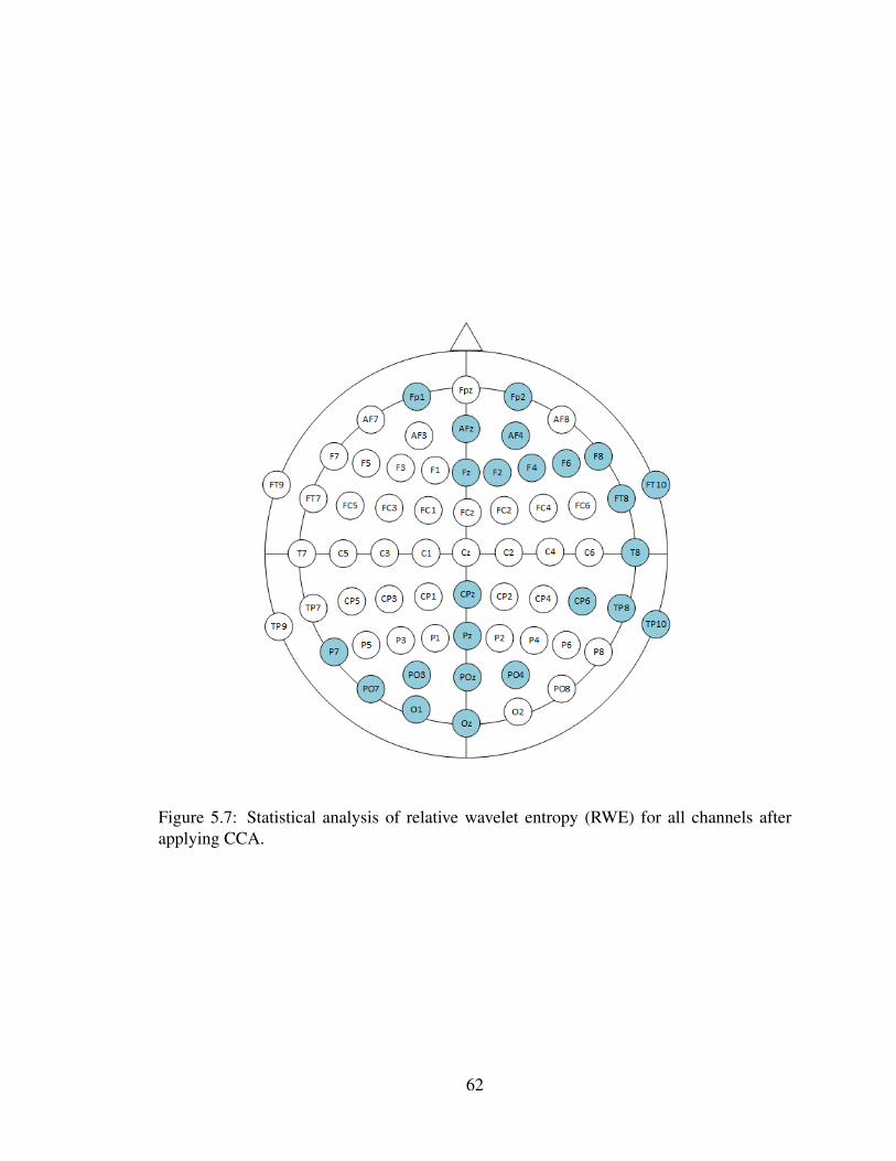
Figure 5.7: Statistical analysis of relative wavelet entropy (RWE) for all channels afterapplying CCA.

62

(a)

(b)

Figure 5.8: Comparison of means (a) and variances (b) of relative Beta2 power for eachchannel after applying ICA.

5.3.2 ICA

After applying ICA method in EEG data, Wilcoxon signed rank test shows that there

is significant difference in test period for P3, P4 and P8 channels. From the right-tailed

hypothesis test, the median beta2 relative power is greater than the median value before the

movement (in P3, P4, P8 and C4 channels).

For all the six channels, Figure 5.8 shows the mean value of relative Beta2 power in

three types of segments. Based on the data we obtained from all eight subjects, it can be

observed that even though ICA method has applied to the original EEG signals, the mean

value in movement-triggered segment is still greater than the other two types of segments.

As for the variance of relative Beta2 power, five channels have the highest variances in

movement-triggered segment except P7, compared with pre-movement and baseline seg-

ment.

63

Figure 5.9: Statistical analysis of relative Beta2 power for all channels after applying ICA.

We also applied the statistical analysis for relative Beta2 power on all channels, the

result is shown in Figure 5.9.

Spectral edge frequency (SEF)

After applying ICA-MARA, Figure 5.10 shows the statistical result of SEF for all chan-

nels in both context period and test period. The significant differences of two channels

(T7 and PO4), which exist in SEF medians between pre-movement segments and baseline

segments, disappear in test period. While there are many other channels which show the

statistical differences.

64

(a)

(b)

Figure 5.10: Statistical analysis of spectral edge frequency (SEF) for all channels in contextperiod (a) and test period (b) after applying ICA.

65

(a)

(b)

Figure 5.11: Comparison of means (a) and variances (b) of wavelet entropy for each chan-nel after applying ICA.

Wavelet entropy

After removing artifact components by using ICA-MARA, the reconstructed signals

are applied for feature extraction.

Figure 5.11 illustrates the mean and variance of wavelet entropy after using ICA for all

six channels, and the comparison in three types of segments. From the result, we could

conclude that when the movement occurs, the variance of WE is significantly larger than

the pre-movement and baseline segments. We have also conducted statistical analysis for

all channels, and the result illustrates that no significant difference exists in wavelet entropy

by Wilcoxon signed rank test.

For further comparison of wavelet entropy, relative wavelet entropy is also applied, in

order to measure the degree of similarity in the reconstructed period and context period.

66

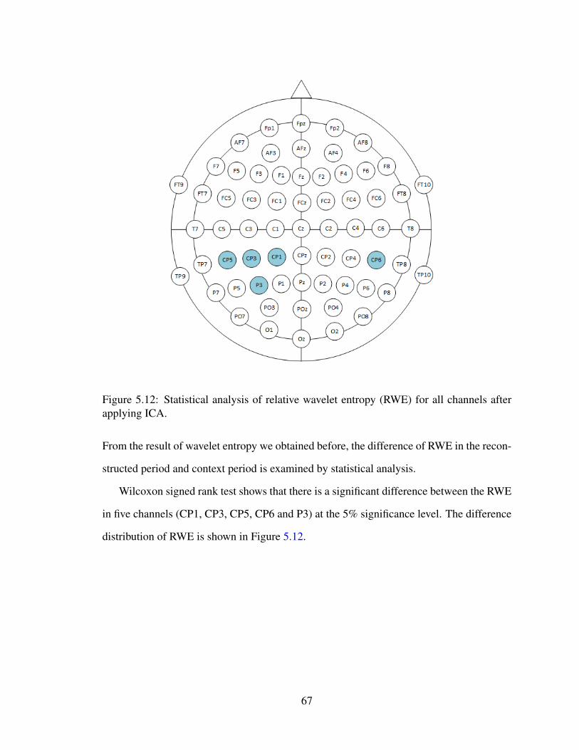
Figure 5.12: Statistical analysis of relative wavelet entropy (RWE) for all channels afterapplying ICA.

From the result of wavelet entropy we obtained before, the difference of RWE in the recon-

structed period and context period is examined by statistical analysis.

Wilcoxon signed rank test shows that there is a significant difference between the RWE

in five channels (CP1, CP3, CP5, CP6 and P3) at the 5% significance level. The difference

distribution of RWE is shown in Figure 5.12.

67

5.4 Discussion

In this chapter, we applied two typical blind source separation (BSS) approaches, namely

canonical correlation analysis (CCA) and independent component analysis (ICA), to re-

move the movement artifacts from EEG signals. However, based on the experimental re-

sults and comparison study, these two methods have not well performed for removing the

movement-triggered artifacts.

After applying CCA method, significant statistical difference of the relative Beta2

power still exist between pre-movement and movement-triggered epochs of all the marked

channels (except C4) in frontal lobe of the scalp. While after ICA, the spatial distribution

of the marked channels changes. Furthermore, according to the RWE feature which is a

way of measuring the degree of similarity, the number of marked channels is reduced. And

the marked channels are obtained by comparing the RWE of a context period and the RWE

of a test period.

Actually, there exist some limitations with the two typical methods for artifact removal.

As for canonical correlation analysis (CCA), it assumes that the autocorrelation of the

sources influenced by movements is lower than the autocorrelation of brain sources. How-

ever, the problem remaining to be discussed is how many sources need to be rejected.

For ICA method, MARA classifier is trained by experts on large dataset, however,

the performance is somehow uncertain in cognitive design process for other movements

in which the classifier was not trained. To discriminate artefactual and neuronal source

components, the problem of which features are suited is essential to deal with. Therefore,

another thing to be argued is the six features used in the classifier construction, which are

probably not the overall optimal choice.

68

Chapter 6

Conclusion and Future Work

6.1 Conclusion

During the course of performing a design task, a variety of movements of the subject

can be generated with or without awareness. The main focus in this research is to analyze

the design-stimulated movements, which are the voluntary short-time movements accom-

panied with the cognitive process, rather than the essential and unavoidable body motions

that are related to answering question and for giving solutions, named as design-related

movements. Based on the video recording, this type of movements is extracted through a

predefined guideline proposed in this thesis.

In the present study, a graphic user interface has been developed, and the effects of un-

specific body motion have been investigated based on statistical differences between signal

features while subjects are working on the cognitive design tasks. Our research results re-

vealed that the relative Beta2 power (20-30Hz) and relative wavelet entropy (RWE) can be

applied to differentiate specific physiological brain states under the background brain ac-

tivities and movement conditions. For the most of channels in the front region of the scalp,

a significant decrease in relative Beta2 power is observed in movement-triggered segments.

Besides, the statistical analysis result of RWE in some channels indicates that the degree

69

of similarity changes when movement occurs. Furthermore, two commonly used meth-

ods, canonical correlation analysis (CCA) and independent component analysis (ICA), are

performed to remove the movement-triggered artifacts, whose performances are evaluated

according to the features in both time and frequency domains. The results indicate that

these two techniques are insufficient to remove these movement artifacts.

As demonstrated by the experimental results, the significant differences between pre-

movement and movement-triggered epochs usually exist in front region of the scalp, which

has, in neuro-physiological field, two main sections in the frontal lobe of primates like

human: prefrontal cortex that is related to cognitive functions, and caudal cortex which is

associated with movement control. The distinction between these two sectors is that the

latter lacks granular cells. This agranular frontal cortex can be further divided into several

anatomically and functionally distinct areas, each of which represents one independent

body movement as reviewed in (Rizzolatti, Luppino, & Matelli, 1998). Recent studies

have shown that motor and premotor cortical regions not only control the preparation and

execution of voluntary movements, but also are engaged in the high level perceptual and

cognitive functions (Rizzolatti & Luppino, 2001) (Mendoza & Merchant, 2014). On the

other hand, body movements can affect the thought in problem solving (Thomas & Lleras,

2009).

Since the two artifact removal techniques have not well performed as we expected, the

feasibility of eliminating the movement-triggered artifacts should be reconsidered. The

definition of artifacts is the potential differences caused by extra-cerebral sources during

EEG tracing, more precisely, either by non-neural physiological activities of human or by

external technical sources. However, when the body movements have an effect on mental

activities, whether the movement-triggered artifacts can still be regarded as non-neural

artifacts or not remains to be discussed and explored.

70

6.2 Future Work

Artifact removal of EEG signal has always been an open and challenging research prob-

lem. In the past few decades, a number of approaches have been developed for achieving

artifact removal in EEG signals. However, it is still difficult to find out a single best method

which is efficient for a wide range of conditions, as it is illustrated in (K. T. Sweeney et al.,

2012). Besides classical techniques in signal processing, such as filtering and blind source

separation, several algorithms which combine two or more currently available methods

have been proposed in recent years. For example, Inuso, Foresta, Mammone, and Mora-

bito (2007) presented a new technique based on the joint use of Wavelet transform and

Independent Component Analysis (WICA), and showed that WICA performs very well

and allows for minimum information loss. After that, ensemble EMD-ICA (EEMD-ICA)

was introduced in (Mijovic, Vos, Gligorijevic, Taelman, & Huffel, 2010), which combines

empirical-mode decomposition with independent component analysis. The performance of

this method is slightly better than WICA in artifact removal simulations.

For future work, the collection of a bigger database with more subjects would be recom-

mended. Since the sources of movements generated by subjects are usually random for the

existing experiments, these body movements of subjects could be divided into several types

for a more detailed analysis. In order to obtain the characteristics of movement-triggered

artifacts, the applicability of more features, apart from the proposed ones, could be in-

vestigated. Moreover, several preliminary experiments for the learning of artifacts could

be conducted before cognitive experiments, for the purpose of investigating the individual

pattern associated with different types of muscle contractions.

Furthermore, the availability of reference signals should be considered when recording

physiological signals. For example, to remove muscle artifact, EMG surface electrodes

could be placed at certain positions during design process. Thus, the recorded EMG sig-

nals will reflect intervals of specific muscle activation, and obtain the delineation of the

71

onset and end time of each movement more precisely. Instead of using video recording

for manual segmentation, which is really time-consuming, EMG signals can provide addi-

tional information and improve the accuracy in time domain. After specifying the epochs

of data samples in the prolonged EEG recordings, methods of signal processing and arti-

fact removal can be applied to these epochs where artifacts are most likely present, with the

consideration of a low computational cost. At the same time, it is also suggested to include

additional electromyographic electrodes as references, especially located over main mus-

cle groups. The collection of EOG signal is also beneficial for the EEG artifact removal

process, and it is extremely important for frontal and temporal lobes of brain.

72

References

Adeli, H., Zhou, Z., & Dadmehr, N. (2003). Analysis of {EEG} records in an epilep-

tic patient using wavelet transform. Journal of Neuroscience Methods, 123(1),

69 - 87. Retrieved from http://www.sciencedirect.com/science/

article/pii/S0165027002003400 doi: http://dx.doi.org/10.1016/S0165

-0270(02)00340-0

Ahmadian, P., Cagnoni, S., & Ascari, L. (2013). How capable is non-invasive eeg data

of predicting the next movement? a mini review. Front Hum Neurosci, 7. (Ah-

madian, Pouya Cagnoni, Stefano Ascari, Luca Front Hum Neurosci. 2013;7:124.

doi:10.3389/fnhum.2013.00124.)

Alexiou, K., Zamenopoulos, T., Johnson, J. H., & Gilbert, S. J. (2009). Exploring the

neurological basis of design cognition using brain imaging: some preliminary results.

Design Studies, 30(6), 623-647. Retrieved from http://www.sciencedirect

.com/science/article/pii/S0142694X09000313

Al-Fahoum, A. S., & Al-Fraihat, A. A. (2014). Methods of eeg signal features extrac-

tion using linear analysis in frequency and time-frequency domains. ISRN Neuro-

science, 2014, 730218. Retrieved from http://www.ncbi.nlm.nih.gov/

pmc/articles/PMC4045570/

Anderer, P., Roberts, S., Schlgl, A., Gruber, G., Klsch, G., Herrmann, W., . . . Saletu, B.

(1999). Artifact processing in computerized analysis of sleep eeg a review. Neu-

ropsychobiology, 40(3), 150-157. Retrieved from http://www.karger.com/

73

http://www.sciencedirect.com/science/article/pii/S0165027002003400


http://www.sciencedirect.com/science/article/pii/S0142694X09000313

http://www.sciencedirect.com/science/article/pii/S0142694X09000313

http://www.ncbi.nlm.nih.gov/pmc/articles/PMC4045570/


http://www.karger.com/DOI/10.1159/000026613


DOI/10.1159/000026613

Berka, C., Levendowski, D. J., Lumicao, M. N., Yau, A., Davis, G., Zivkovic, V. T., . . .

Craven, P. L. (2007). Eeg correlates of task engagement and mental workload in vig-

ilance, learning, and memory tasks. Aviation, Space, and Environmental Medicine,

78(5), B231-B244.

Berka, C., Levendowski, D. J., Westbrook, P., Davis, G., Lumicao, M. N., Olmstead, R. E.,

. . . Ramsey, C. K. (2005). Eeg quantification of alertness: methods for early identifi-

cation of individuals most susceptible to sleep deprivation. , 5797, 78-89. Retrieved

from http://dx.doi.org/10.1117/12.597503

Brittenham, D. (1974). Recognition and reduction of physiological artifacts. American

Journal of EEG Technology, 14(2-3), 158-165.

Carskadon, M. A., & Rechtschaffen, A. (2000). Monitoring and staging human sleep.

Principles and practice of sleep medicine, 3, 1197-1215.

Clercq, W. D., Vergult, A., Vanrumste, B., Paesschen, W. V., & Huffel, S. V. (2006).

Canonical correlation analysis applied to remove muscle artifacts from the electroen-

cephalogram. IEEE Transactions on Biomedical Engineering, 53(12), 2583-2587.

Cohen, B. H., Davidson, R. J., Senulis, J. A., Saron, C. D., & Weisman, D. R. (1992).

Muscle tension patterns during auditory attention. Biological Psychology, 33(23),

133-156. Retrieved from http://www.sciencedirect.com/science/

article/pii/030105119290028S

Committee, E. P. N. (1994). Guideline thirteen: guidelines for standard electrode position

nomenclature. J Clin Neurophysiol, 11, 111-3.

Conforto, S., D’Alessio, T., & Pignatelli, S. (1999). Optimal rejection of

movement artefacts from myoelectric signals by means of a wavelet filter-

ing procedure. Journal of Electromyography and Kinesiology, 9(1), 47 - 57.

Retrieved from http://www.sciencedirect.com/science/article/

74



http://dx.doi.org/10.1117/12.597503

http://www.sciencedirect.com/science/article/pii/030105119290028S

http://www.sciencedirect.com/science/article/pii/030105119290028S



pii/S1050641198000236 doi: http://dx.doi.org/10.1016/S1050-6411(98)

00023-6

Croft, R. J., & Barry, R. J. (2000). Removal of ocular artifact from the eeg: a review.

Neurophysiologie Clinique/Clinical Neurophysiology, 30(1), 5-19. doi: http://dx.doi

.org/10.1016/S0987-7053(00)00055-1

Croft, R. J., & Barry, R. J. (2002). Issues relating to the subtraction phase in eog artefact

correction of the eeg. International Journal of Psychophysiology, 44(3), 187-195.


pii/S016787600100201X

Deecke, L., Scheid, P., & Kornhuber, H. H. (1969). Distribution of readiness potential, pre-

motion positivity, and motor potential of the human cerebral cortex preceding volun-

tary finger movements. Experimental Brain Research, 7(2), 158–168. Retrieved from

http://dx.doi.org/10.1007/BF00235441 doi: 10.1007/BF00235441

Delorme, A., & Makeig, S. (2004). Eeglab: an open source toolbox for analysis of single-

trial {EEG} dynamics including independent component analysis. Journal of Neuro-

science Methods, 134(1), 9 - 21. Retrieved from //www.sciencedirect.com/

science/article/pii/S0165027003003479 doi: http://dx.doi.org/10

.1016/j.jneumeth.2003.10.009

Farina, D., do Nascimento, O. F., Lucas, M.-F., & Doncarli, C. (2007). Optimiza-

tion of wavelets for classification of movement-related cortical potentials gener-

ated by variation of force-related parameters. Journal of Neuroscience Methods,

162(12), 357 - 363. Retrieved from http://www.sciencedirect.com/

science/article/pii/S0165027007000362 doi: http://dx.doi.org/10

.1016/j.jneumeth.2007.01.011

Fatourechi, M., Bashashati, A., Ward, R. K., & Birch, G. E. (2007). Emg and eog

75



http://www.sciencedirect.com/science/article/pii/S016787600100201X


http://dx.doi.org/10.1007/BF00235441

//www.sciencedirect.com/science/article/pii/S0165027003003479




artifacts in brain computer interface systems: A survey. Clinical Neurophysiol-

ogy, 118(3), 480-494. Retrieved from http://www.sciencedirect.com/

science/article/pii/S1388245706015124

Gazzaniga, M. S. (1989). Organization of the human brain. Science, 245(4921), 947-952.

Gevins, A., & Smith, M. E. (2003). Neurophysiological measures of cognitive

workload during human-computer interaction. Theoretical Issues in Ergonomics

Science, 4(1-2), 113-131. Retrieved from http://dx.doi.org/10.1080/

14639220210159717

Gevins, A., Smith, M. E., Leong, H., McEvoy, L., Whitfield, S., Du, R., & Rush, G.

(1998). Monitoring working memory load during computer-based tasks with eeg

pattern recognition methods. Human Factors: The Journal of the Human Factors

and Ergonomics Society, 40(1), 79-91.

Goljahani, A., D’Avanzo, C., Schiff, S., Amodio, P., Bisiacchi, P., & Sparacino, G.

(2012). A novel method for the determination of the eeg individual alpha frequency.

NeuroImage, 60(1), 774-786. Retrieved from http://www.sciencedirect

.com/science/article/pii/S105381191101398X

Goncharova, I., McFarland, D., Vaughan, T., & Wolpaw, J. (2003). {EMG} contamination

of eeg: spectral and topographical characteristics. Clinical Neurophysiology, 114(9),

1580 - 1593. Retrieved from http://www.sciencedirect.com/science/


-2457(03)00093-2

Guo, L., Rivero, D., Seoane, J. A., & Pazos, A. (2009). Classification of eeg signals us-

ing relative wavelet energy and artificial neural networks. In Proceedings of the first

acm/sigevo summit on genetic and evolutionary computation (pp. 177–184). New

York, NY, USA: ACM. Retrieved from http://doi.acm.org/10.1145/

1543834.1543860 doi: 10.1145/1543834.1543860

76



http://dx.doi.org/10.1080/14639220210159717

http://dx.doi.org/10.1080/14639220210159717





http://doi.acm.org/10.1145/1543834.1543860

http://doi.acm.org/10.1145/1543834.1543860

Howells, F. M., Stein, D. J., & Russell, V. A. (2010). Perceived mental effort cor-

relates with changes in tonic arousal during attentional tasks. Behavioral and

Brain Functions, 6(1), 39. Retrieved from http://dx.doi.org/10.1186/

1744-9081-6-39

Huigen, E., Peper, A., & Grimbergen, C. A. (2002). Investigation into the origin of the noise

of surface electrodes. Medical and Biological Engineering and Computing, 40(3),

332-338. Retrieved from http://dx.doi.org/10.1007/BF02344216

Hyvrinen, A., & Oja, E. (2000). Independent component analysis: algo-

rithms and applications. Neural Networks, 13(45), 411 - 430. Retrieved

from http://www.sciencedirect.com/science/article/pii/

S0893608000000265 doi: http://dx.doi.org/10.1016/S0893-6080(00)00026-5

Inuso, G., Foresta, F. L., Mammone, N., & Morabito, F. C. (2007, Aug). Wavelet-ica

methodology for efficient artifact removal from electroencephalographic recordings.

In 2007 international joint conference on neural networks (p. 1524-1529). doi: 10

.1109/IJCNN.2007.4371184

Jasper, H. H. (1958). The ten twenty electrode system of the international federation.

Electroencephalography and Clinical Neurophysiology, 10, 371-375. Retrieved from

http://ci.nii.ac.jp/naid/10020218106/en/

Jung, T.-P., Makeig, S., Humphries, C., Lee, T.-W., McKeown, M. J., Iragui, V., & Se-

jnowski, T. J. (2000). Removing electroencephalographic artifacts by blind source

separation. Psychophysiology, 37(2), 163–178. Retrieved from http://dx.doi

.org/10.1111/1469-8986.3720163 doi: 10.1111/1469-8986.3720163

Klass, D. W. (1995). The continuing challenge of artifacts in the eeg. American Journal of

EEG Technology, 35(4), 239-269. Retrieved from http://www.tandfonline

.com/doi/abs/10.1080/00029238.1995.11080524

Kline, J. E., Huang, H. J., Snyder, K. L., & Ferris, D. P. (2015). Isolating gait-related

77

http://dx.doi.org/10.1186/1744-9081-6-39

http://dx.doi.org/10.1186/1744-9081-6-39

http://dx.doi.org/10.1007/BF02344216



http://ci.nii.ac.jp/naid/10020218106/en/

http://dx.doi.org/10.1111/1469-8986.3720163

http://dx.doi.org/10.1111/1469-8986.3720163

http://www.tandfonline.com/doi/abs/10.1080/00029238.1995.11080524

http://www.tandfonline.com/doi/abs/10.1080/00029238.1995.11080524

movement artifacts in electroencephalography during human walking. Journal of

neural engineering, 12(4), 046022-046022. (26083595[pmid] J Neural Eng)

Kornhuber, H. H., & Deecke, L. (1965). Hirnpotentialanderungen bei willkurbewegungen

und passiven bewegungen des menschen: Bereitschaftspotential und reafferente po-

tentiale. Pfluger’s Archiv fur die gesamte Physiologie des Menschen und der Tiere,

284(1), 1–17. Retrieved from http://dx.doi.org/10.1007/BF00412364

doi: 10.1007/BF00412364

Kumar, Y., Dewal, M. L., & Anand, R. S. (2012). Relative wavelet energy and wavelet

entropy based epileptic brain signals classification. Biomedical Engineering Let-

ters, 2(3), 147–157. Retrieved from http://dx.doi.org/10.1007/s13534

-012-0066-7 doi: 10.1007/s13534-012-0066-7

Luck, S. J. (2005). Ten simple rules for designing erp experiments. Event-related poten-

tials: A methods handbook, 262083337.

Mallat, S. G. (1989). A theory for multiresolution signal decomposition: the wavelet

representation. IEEE Transactions on Pattern Analysis and Machine Intelligence,

11(7), 674-693.

McFarland, D. J., Sarnacki, W. A., Vaughan, T. M., & Wolpaw, J. R.

(2005). Brain-computer interface (bci) operation: signal and noise dur-

ing early training sessions. Clinical Neurophysiology, 116(1), 56-62.


pii/S1388245704002664

McGrogan, N., et al. (1999). Neural network detection of epileptic seizures in the elec-

troencephalogram.

Mendoza, G., & Merchant, H. (2014). Motor system evolution and the emer-

gence of high cognitive functions. Progress in Neurobiology, 122, 73 -

93. Retrieved from //www.sciencedirect.com/science/article/

78

http://dx.doi.org/10.1007/BF00412364

http://dx.doi.org/10.1007/s13534-012-0066-7

http://dx.doi.org/10.1007/s13534-012-0066-7





pii/S0301008214000999 doi: http://dx.doi.org/10.1016/j.pneurobio.2014.09

.001

Mijovic, B., Vos, M. D., Gligorijevic, I., Taelman, J., & Huffel, S. V. (2010, Sept). Source

separation from single-channel recordings by combining empirical-mode decompo-

sition and independent component analysis. IEEE Transactions on Biomedical En-

gineering, 57(9), 2188-2196. doi: 10.1109/TBME.2010.2051440

Mulert, C., Menzinger, E., Leicht, G., Pogarell, O., & Hegerl, U. (2005). Evidence for

a close relationship between conscious effort and anterior cingulate cortex activity.

International Journal of Psychophysiology, 56(1), 65-80.

Nguyen, T. A., & Zeng, Y. (2012). Clustering designers mental activities based on eeg

power. Tools and methods of competitive engineering, Karlsruhe, Germany.

Nguyen, T. A., & Zeng, Y. (2014). A physiological study of relationship between designers

mental effort and mental stress during conceptual design. Computer-Aided Design,

54, 3-18. Retrieved from http://www.sciencedirect.com/science/

article/pii/S0010448513002005

Nguyen, T. A., & Zeng, Y. (2016). Effects of stress and effort on self-rated reports in

experimental study of design activities. Journal of Intelligent Manufacturing, 1-14.

Retrieved from http://dx.doi.org/10.1007/s10845-016-1196-z

Niedermeyer, E., & da Silva, F. L. (2005). Electroencephalography: basic principles,

clinical applications, and related fields. Lippincott Williams and Wilkins.

Regan, S. O., Faul, S., & Marnane, W. (2010). Automatic detection of eeg artefacts

arising from head movements. In 2010 annual international conference of the ieee

engineering in medicine and biology (p. 6353-6356).

Reis, P. M. R., Hebenstreit, F., Gabsteiger, F., von Tscharner, V., & Lochmann, M. (2014).

Methodological aspects of eeg and body dynamics measurements during motion.

79





http://dx.doi.org/10.1007/s10845-016-1196-z

Front Hum Neurosci, 8. (Reis, Pedro M R Hebenstreit, Felix Gabsteiger, Flo-

rian von Tscharner, Vinzenz Lochmann, Matthias Front Hum Neurosci. 2014;8:156.

doi:10.3389/fnhum.2014.00156.)

Ribas, G. C. (2010). The cerebral sulci and gyri. Neurosurgical focus, 28(2), E2.

Rizzolatti, G., & Luppino, G. (2001). The cortical motor system. Neuron, 31(6), 889

- 901. Retrieved from //www.sciencedirect.com/science/article/

pii/S0896627301004238 doi: http://dx.doi.org/10.1016/S0896-6273(01)

00423-8

Rizzolatti, G., Luppino, G., & Matelli, M. (1998). The organization of the cortical mo-

tor system: new concepts. Electroencephalography and Clinical Neurophysiology,

106(4), 283 - 296. Retrieved from //www.sciencedirect.com/science/


-4694(98)00022-4

Rosso, O. A., Blanco, S., & Figliola, A. (2004). Characterization of the dynami-

cal evolution of electroencephalogram time series. In O. Descalzi, J. Martınez, &

E. Tirapegui (Eds.), Instabilities and nonequilibrium structures vii & viii (pp. 333–

338). Dordrecht: Springer Netherlands. Retrieved from http://dx.doi.org/

10.1007/978-1-4020-2149-7 24 doi: 10.1007/978-1-4020-2149-7 24

Rosso, O. A., Blanco, S., Yordanova, J., Kolev, V., Figliola, A., Schrmann, M., & Baar, E.

(2001). Wavelet entropy: a new tool for analysis of short duration brain electrical

signals. Journal of Neuroscience Methods, 105(1), 65-75.

Schacter, D. L. (1977). Eeg theta waves and psychological phenomena: A review

and analysis. Biological Psychology, 5(1), 47-82. Retrieved from http://www

.sciencedirect.com/science/article/pii/030105117790028X

Schwender, D., Daunderer, M., Mulzer, S., Klasing, S., Finsterer, U., & Peter, K. (1996).

80





http://dx.doi.org/10.1007/978-1-4020-2149-7_24

http://dx.doi.org/10.1007/978-1-4020-2149-7_24

http://www.sciencedirect.com/science/article/pii/030105117790028X

http://www.sciencedirect.com/science/article/pii/030105117790028X

Spectral edge frequency of the electroencephalogram to monitor” depth” of anaes-

thesia with isoflurane or propofol. British journal of anaesthesia, 77(2), 179-184.

Shibasaki, H., & Hallett, M. (2006). What is the bereitschaftspotential? Clinical Neu-

rophysiology, 117(11), 2341 - 2356. Retrieved from //www.sciencedirect

.com/science/article/pii/S138824570600229X doi: http://dx.doi

.org/10.1016/j.clinph.2006.04.025

Solomon Jr, O. M. (1991). Psd computations using welch’s method.[power spectral density

(psd)] (Tech. Rep.). Sandia National Labs., Albuquerque, NM (United States).

Sornmo, L., & Laguna, P. (2005). Chapter 3 - eeg signal processing. In Bioelectrical signal

processing in cardiac and neurological applications (p. 55-179). Burlington: Aca-

demic Press. Retrieved from http://www.sciencedirect.com/science/

article/pii/B9780124375529500039

Sweeney, K., McLoone, S., & Ward, T. (2010). A simple bio-signals quality measure for

in-home monitoring.

Sweeney, K. T., Ward, T. E., & McLoone, S. F. (2012, May). Artifact removal in physio-

logical signals: Practices and possibilities. IEEE Transactions on Information Tech-

nology in Biomedicine, 16(3), 488-500. doi: 10.1109/TITB.2012.2188536

Tang, Y., & Zeng, Y. (2009). Quantifying designers mental stress in the conceptual design

process using kinesics study. In Ds 58-9: Proceedings of iced 09, the 17th interna-

tional conference on engineering design, vol. 9, human behavior in design, palo alto,

ca, usa, 24.-27.08. 2009.

Teplan, M. (2002). Fundamentals of eeg measurement. Measurement science review, 2(2),

1-11.

Thomas, L. E., & Lleras, A. (2009). Swinging into thought: Directed movement

guides insight in problem solving. Psychonomic Bulletin & Review, 16(4), 719–

723. Retrieved from http://dx.doi.org/10.3758/PBR.16.4.719 doi:

81

//www.sciencedirect.com/science/article/pii/S138824570600229X

//www.sciencedirect.com/science/article/pii/S138824570600229X

http://www.sciencedirect.com/science/article/pii/B9780124375529500039

http://www.sciencedirect.com/science/article/pii/B9780124375529500039

http://dx.doi.org/10.3758/PBR.16.4.719

10.3758/PBR.16.4.719

Van de Velde, M., van Erp, G., & Cluitmans, P. J. M. (1998). Detection of muscle artefact

in the normal human awake eeg. Electroencephalography and Clinical Neurophysi-

ology, 107(2), 149-158. Retrieved from http://www.sciencedirect.com/

science/article/pii/S0013469498000522

Walter, W. (1953). The living brain.

Welch, P. D. (1967). The use of fast fourier transform for the estimation of power spec-

tra: A method based on time averaging over short, modied periodograms. IEEE

Transactions on audio and electroacoustics, 15(2), 70-73.

Winkler, I., Haufe, S., & Tangermann, M. (2011). Automatic classification of artifactual

ica-components for artifact removal in eeg signals. Behavioral and Brain Functions,

7(1), 1-15. Retrieved from http://dx.doi.org/10.1186/1744-9081-7

-30

Wolpaw, J. R., & McFarland, D. J. (2004). Control of a two-dimensional move-

ment signal by a noninvasive brain-computer interface in humans. Proceed-

ings of the National Academy of Sciences of the United States of America,

101(51), 17849-17854. Retrieved from http://www.ncbi.nlm.nih.gov/

pmc/articles/PMC535103/

Woodman, G. F. (2010). A brief introduction to the use of event-related potentials (erps) in

studies of perception and attention. Attention, perception and psychophysics, 72(8),

10.3758/APP.72.8.2031. Retrieved from http://www.ncbi.nlm.nih.gov/

pmc/articles/PMC3816929

82



http://dx.doi.org/10.1186/1744-9081-7-30

http://dx.doi.org/10.1186/1744-9081-7-30



http://www.ncbi.nlm.nih.gov/pmc/articles/PMC3816929

http://www.ncbi.nlm.nih.gov/pmc/articles/PMC3816929

Artifact Analysis and Removal of Electroencephalographic ... · PDF fileArtifact Analysis and...

Documents

Transcript of Artifact Analysis and Removal of Electroencephalographic ... · PDF fileArtifact Analysis and...