Articol-conferinta Brasov Nov 2014

PROCEEDINGS OF THE INTERNATIONAL

SCIENTIFIC CONFERENCE

CIBv 2014

7th-8th of NOVEMBER

TRANSILVANIA UNIVERSITY PUBLISHING HOUSE

BRAŞOV

3

TRANSILVANIA UNIVERSITY OF BRAŞOV

CIVIL ENGINEERING FACULTY

and

ROMANIAN ASSOCIATION OF BUILDING SERVICES ENGINEERS (AIIR)

under the high patronage of the

ROMANIAN ACADEMY OF TECHNICAL SCIENCES

Section of

CIVIL ENGINEERING AND URBANISM

CIBv 2014

Proceedings of the

INTERNATIONAL SCIENTIFIC CONFERENCE

7th-8th of NOVEMBER 2014

Braşov

TRANSILVANIA UNIVERSITY PUBLISHING HOUSE

2014

4

©2013 EDITURA UNIVERSITĂŢII TRANSILVANIA BRAŞOV

Adress: 500091 Braşov, B-dul Iuliu Maniu 41A Tel. 0268-476050 Fax 0268-476051 E-mail: [email protected]

Published at: Transilvania University publishing house from Brasov B-dul Eroilor 9 tel/fax 0268-475348 All rights are rezerved Editură acreditată CNCSIS Adress nr. 1615 din 29 mai 2002

EDITORS: Prof.univ.dr.ing. Ioan TUNS [email protected] Conf.dr.ing. Valentin-Vasile UNGUREANU [email protected] Şef lucr.dr.ing. Florin-Lucian TĂMAŞ,

[email protected]

ISSN 2285-7656 ISSN-L 2248-7648

5

INTERNATIONAL ACADEMIC SCIENTIFIC COMMITTEE

Prof. PhD. Eng. Ioan TUNS – Chairman – U. Transilvania Braşov, Romania Prof. Dr. Eng. Gheorghe BADEA Prof. Dr. Eng. Radu BĂNCILĂ Prof. Dr. Eng. Miroslav BEŠEVIĆ Dr. Eng. Peter BLOOMFIELD Prof. Dr. Eng. Ioan BOIAN Prof. Dr. Eng. Ioan BORZA Ass. Prof. Dr. Eng. Marius Florin BOTIŞ Prof. Dr. Eng. Mihai BUDESCU Prof. Dr. Eng. Jan BUJNAK Prof. Dr. Eng. Sorin BURCHIU Ass. Prof. Dr. Eng. Mircea Ion BUZDUGAN Prof. Dr. Eng. Sorin CALUIANU Ass. Prof. Dr. Eng. Vasilică CIOCAN Ass. Prof. Dr. Eng. Lucian CÎRSTOLOVEAN Prof. Dr. Eng. Fulvio CHIMISSO Ass. Prof. Dr. Eng. Nicolae CHIRA Prof. Dr. Eng. Florea CHIRIAC Prof. Dr. Eng. Vasile CIOFOAIA Prof. Dr. Eng. Ioan CURTU Prof. Dr. Eng. Mircea Radu DAMIAN Ass. Prof. Dr. Eng. Nicolae DĂSCĂLESCU Prof. Dr. Eng. Mihai DICU Dr. Eng. Ioan Silviu DOBOŞI Prof. Dr. Eng. Victor DOGARU Ass. Prof. Dr. Eng. Gheorghe Viorel DRAGOŞ Prof. Dr. Eng. Liviu DRUGHEAN Prof. Dr. Eng. Liviu DUMITRESCU Prof. Dr. Eng. Josef FINK Prof. Dr. Eng. Nicolae FLOREA Prof. Dr. Eng. Radomir FOLIC Prof. Dr. Eng. Wolfgang FRANCKE Prof. Dr. Eng. Rodica FRUNZULICĂ Ass. Prof. Dr. Eng. Ionel GOSAV Prof. Dr. Eng. Liviu GROLL Ass. Prof. Dr. Eng. Mircea HORNEŢ Prof. Dr. Eng. Jan IGNAT Prof. Dr. Eng. Mihai ILIESCU Prof. Dr. Eng. Miklós IVÁNYI

Ass. Prof. Dr. Eng. Eva KORMANÍKOVÁ Ass. Prof. Dr. Eng. Kamila KOTRASOVÁ Prof. Dr. Eng. Danijel KUKARAS Prof. Dr. Eng. Gheorghe LUCACI Ass. Prof. Dr. Eng. Cătălin LUNGU Prof. Dr. Eng. Aurora-Carmen MANCIA Prof. Dr. Eng. James R. MARTIN, II Prof. Dr. Eng. Teodor MATEESCU Ass. Prof. Dr. Eng. Carmen MÎRZA Ass. Prof. Dr. Eng. Gavrilă MUNTEAN Ass. Prof. Dr. Eng. Guney OLGUN Ass. Prof. Dr. Eng. Eduard PETZEK Dr. Eng. Victor POPA Prof. Dr. Eng. Augustin POPĂESCU Ass. Prof. Dr. Eng. Marcela PRADA Prof. Dr. Eng. Dan PRECUPANU Prof. Dr. Eng. Daniela PREDA Prof. Dr. Eng. Vlastimir RADONJANIN Prof. Dr. Eng. Constantin RADU Dr. Eng. Andrei RÂMNICEANU Prof. Dr. Eng. Wolfgang REITMEIER Prof. Dr. Eng. Adrian RETEZAN Prof. Dr. Eng. Horea SANDI Prof. Dr. Eng. Aleksandar SEDMAK Prof. Dr. Eng. Mike SIEDER Prof. Dr. Eng. Dan STEMATIU Prof. Dr. Eng. Bratislav STIPANICI Prof. Dr. Eng. Alexandru ŞERBAN Prof. Dr. Eng. Nicolae ŢĂRANU Prof. Dr. Eng. Kostadin Hristev TOPUROV Ass. Prof. Dr. Eng. Valentin-Vasile UNGUREANU Prof. Dr. Eng. Marina VERDEȘ Prof. Dr. Eng. Horst WERKLE Prof. Dr. Eng. Thomas WUNDERLICH Prof. Dr. Eng. Nesrin YARDIMCI Prof. Dr. Eng. Eberhard ZOLLER Prof. Dr. Eng. Miroslav ŽIVKOVIC

HONORARY COMMITTEE:

Prof. Dr. Eng. Ioan Vasile ABRUDAN Rector of Transilvania University Braşov

Prof. Dr. Eng. Dan STEMATIU President of Civil Engineering and Urbanism section of the

Romanian Academy of Technical Sciences and Professor of Technical University of Civil Engineering of Bucharest

Prof. Dr. Eng. Horea SANDI Honorary professor and

Doctor Honoris Causa of Technical University of Civil Engineering of Bucharest

Eng. Michel COUILLARD

ORGANIZING COMMITTEE:

Chairman: Prof. Dr. Eng. Ioan TUNS

Dean of Civil Engineering Faculty of Braşov

Members: Prof. Dr. Eng. Ioan BOIAN Prof. Dr. Eng. Math. Vasile CIOFOAIA Prof. Dr. Eng. Alexandru ŞERBAN Ass. Prof. Dr. Eng. Marius Florin BOTIŞ Ass. Prof. Dr. Lucian CÎRSTOLOVEAN Ass. Prof. Dr. Eng. Nicolae DĂSCĂLESCU Ass. Prof. Dr. Eng. Adam DÓSA Ass. Prof. Dr. Eng. Mircea HORNEŢ Ass. Prof. Dr. Eng. Marius MĂNTULESCU Ass. Prof. Dr. Eng. Gavril MUNTEAN Ass Prof. Dr. Eng. Valentin-Vasile UNGUREANU Lecturer Dr. Eng. Lucia BOERIU Lecturer Dr. Eng. Christiana-Emilia CAZACU Lecturer Dr. Eng. Dumitru CHISALIŢĂ Lecturer Dr. Arh. Cristina CHIŢONU Lecturer Eng. Marius COMĂNICI Lecturer Dr. Eng. Ovidiu DEACONU

Lecturer Dr. Eng. Mariana FRATU Lecturer Dr. Eng. Teofil-Florin GĂLĂŢANU Lecturer Dr. Eng. Nicolae IORDAN Lecturer Dr. Eng. Sorin LEOVEANU Lecturer Dr. Eng. Paraschiva MIZGAN Lecturer Dr. Eng. Radu MUNTEAN Lecturer Dr. Eng. Florin-Lucian TĂMAŞ Assist. Eng. Ciprian CISMAŞ Assist. Eng. George DRAGOMIR Assist. Eng. Petre IOSUB Assist. Eng. Cristian NĂSTAC Assist. Eng. Lucian POPA Assist. Eng. Dorin RADU Assist. Dr. Eng. Daniel TAUS Tutor Eng. Sorin BOLOCAN Tutor Dr. Eng. Gabriel NĂSTASE

TOPICS

1. Structural analysis and optimization 2. Reinforced concrete structures 3. Steel structures 4. Wood structures 5. Computer aided design of structures 6. Railways, roads and bridges 7. Geotechnics and foundations 8. Consolidation of buildings 9. Experimental methods in investigation of structures 10. Advanced energy design for HVAC installations 11. Energy performance of buildings and installations 12. Efficient buildings based on renewable energy 13. High performance lighting systems for buildings 14. New materials and technologies in building industry

INTERNATIONAL SCIENTIFIC CONFERENCE CIBv 2014 7-8 November 2014, Braşov

SUMMARY

BUILDING SERVICES

S. BOLOCAN, A. SERBAN, F. CHIRIAC, I. BOIAN, V. CIOFOAIA -

Performance evaluation of a small capacity solar cooling ARS..............................1

B. BRĂNIȘTEANU, D. M. ȘERBAN, D. D. SOLOMON - Analisys of

predicted sprinkler activation time in automated car parkings ................................9

M. BUZDUGAN, H. BĂLAN - On electrical energy efficiency in buildings .....15

T. V. CHIRA - Faults found in sewer pipes, causes and remedies.......................23

G. CORSIUC, C. MÂRZA, R. FELSEGHI, T. ŞOIMOŞAN,

M. ROMAN - Analysis of using stand-alone solar-wind power

system in rural areas ..............................................................................................31

G. DRAGOMIR, A. BREZEANU, V. CIOFOAIA - Experimental research

on the temperature distribution of thermally activated building systems (tabs)....39

G. DRAGOMIR, G. NASTASE, V. CIOFOAIA, I. BOIAN,

A. SERBAN, A. BREZEANU - The impact of design parameters on

the cooling performance of TABS.........................................................................45

G. DRAGOȘ, R. MOLDOVAN - Efficient ways of providing thermal

energy to passive houses........................................................................................53

V. S. HUDISTEANU, A. I. BARAN, M. BALAN, N. C. CHERECHES,

T. MATEESCU, M. VERDES, V. CIOCAN - Improvement of the indoor

climate conditions inside orthodox churches.........................................................61

V. IACOB - The impact of the site organization on the environment ..................67

C. MÂRZA, G. CORSIUC, D. ILUŢIU-VARVARA - Consideration

on biomass valorization .........................................................................................73

R. MOLDOVAN, G. DRAGOŞ - The influence of enveloping on

energetic and ecological efficiency of passive houses...........................................81 G. NĂSTASE, A. ŞERBAN - Comsol Multiphysicstm as an educational

resource for students ..............................................................................................89

M. PROFIRE, A. BURLACU - Efficient management of the drinking

water distribution system in the city of Iasi ...........................................................93

M. PROFIRE, A. BURLACU - Water loss reduction through on-line

monitoring of physical and chemical parameters ..................................................99

A. RETEZAN, S. Z. GEYER EHRENBERG, C. PĂCURAR - Solutions

of energy optimisation in industrial plants ..........................................................103 D.S. RUSU - Prediction of energy consumption in residential buildings

before and after retrofiting using artificial neural networks ................................111 G. TARLEA, M. VINCERIUC, A. TARLEA - Theoretical ecological

study -refrigerant comparison-.............................................................................117

CIVIL ENGINEERING,

RAILWAYS, ROADS AND BRIDGES

I. BADEA, D. BADEA - Infrastructure behavior of existing steel

bridges in operation .............................................................................................121

R. BĂNCILĂ, D. BOLDUȘ, A. FEIER, S. HERNEA, M. MALIȚA -

Deflection and precambering of steel beams .................................................... 127

R. BĂNCILĂ, A. FEIER, D. RADU - Rehabilitation of existing

steel structures, an integral part of the sustainable development....................... 137

A.D. BERINDEAN, C.A. BERINDEAN - Experimental study regarding

the behavior of glue laminated beams double reinforced with rectangular

metal pipes (RMP) ...............................................................................................143

V. BOBOC, A. BOBOC - Modernization solutions for local roads ..................149

A.C. BOJAN, A. CHIRA - Numerical and experimental investigations

on the behavior of thermosystem subjected to wind loads .................................155

C. CAZACU - A few aspects about the national building code .........................161

D. M. COSTEA, M. N. GĂMAN, G. DUMITRU - On the structure

of molded steel thermic........................................................................................167

D. M. COSTEA, M. N. GĂMAN, G. DUMITRU - The weld

aluminothermic optimization of rail track by microalloyed ................................173

D. COVATARIU, R.G. ŢARAN, D. COVATARIU - The influence to

the impact strength of the recycled rubber granules addition on the

concrete structural elements.................................................................................177

D. COVATARIU, D.T. BABOR, R.G. ŢARAN - Multicriteria

comparative analysis on the effectiveness use of various materials

for thermal insulation in romanian residential buildings .....................................185

G. DAE, M. CARABINEANU, G. DUMITRU - The stages of

authorization for placing in service .....................................................................195

O. DEACONU - Conditions of the constructions sustainability in

natural environments............................................................................................205

G. DIMA, V. V. UNGUREANU - Design and verification of a testing

interface for axial and bending loading of the structural T joints........................209

C. F. DOBRESCU, E. A. CALARASU, V.V. UNGUREANU - Similarity

topics of soils with sensitivity to wetting based upon data gathered from

laboratory tests .....................................................................................................217

G. DUMITRU, V. ŞTEFAN, M. LITRĂ, E. CRĂCIUN BOJE,

C. N. BADEA, G. M. DRAGNE - Dynamic study on safety against the

derailment to the six axle locomotives ................................................................223

G. DUMITRU, L. BLAGA, G. A. BADEA, E. CRĂCIUN BOJE,

C. N. BADEA, G. M. DRAGNE, V. ŞTEFAN - The vertical loads

variations study and the guidance capacity of six axle locomotives

at curves circulation .............................................................................................231

N. ĐURIĆ - Analysis of geotechnical conditions for construction of

desulphurization of thermal power plant Ugljevik 1 ...........................................247

M. FETEA - Application of the Galerkin-Vlasov variational method

in the study of free vibrations of the square plate C-C-SF-F...............................255

A. FIRUS, H. WERKLE, W. FRANCKE, C. CLAUSNER - Evaluation

of footfall-induced vibrations and their importance in a biomechanics

laboratory .............................................................................................................263

Z. C. GRIGORAŞ - Analysing the human behavior in a fire drill.

comparison between two evacuation software: FDS+EVAC and Pathfinder .....273

Z. C. GRIGORAŞ, D. DIACONU-ŞOTROPA - Fire resistance assessment

according to the thermal insulation criterion – an engineering approach............281

E. KORMANÍKOVÁ, K. KOTRASOVÁ - Dynamic response of

a composite beam.................................................................................................289

D. KUKARAS, M. BEŠEVIĆ, A. PROKIĆ, D. NADAŠKI - Testing

and numerical modeling - steel truss of the sports hall........................................295

A. LANDOVIĆ, M. BEŠEVIĆ - Analysis of ultimate load capacity

of short RC and composite columns ....................................................................301

D.F. LIŞMAN - Wireless sensor network used for structural health

monitoring of civil infrastructure.........................................................................307

M. MĂNTULESCU, I. TUNS, F-L. TĂMAŞ - Correlation of some

parameters “in situ” determined during executions of

Ghimbav-Braşov runway airport .........................................................................317

T. MILCHIȘ, I. BORŞ - Behaviour of elevated concrete water tower

under dynamic loads ............................................................................................323

R. NERIŞANU, D. DRĂGAN, M. SUCIU - Study of effects of

vibrations caused by railway traffic to buildings.................................................329

D. OANEA (FEDIUC), M. BUDESCU, V. M. VENGHIAC - Conditions

regarding the use of elastomeric bearings in base isolation.................................337

E-L. PLESCAN, C. PLESCAN - Implementation of mechanistic empirical

pavement design guide Me-Pdg in Romania .......................................................345

C. POPA - Integrated design, the solution for saving time, energy,

resources and CO2................................................................................................351

G. POPA, C.N. BADEA, A. BADEA - Pneumatic air springs for

railway vehicles ...................................................................................................359

D. PREDA, S.I. MINEA - Bolted connections on circular end plates ...............365

A. PROKIC, M. VOJNIC PURCAR, D. LUKIC - A new finite element

considering shear lag ...........................................................................................371

D. RADU, A. SEDMAK - Failure modes and designing procedures

of the tubular truss beams welded joints according with en 1993-1-8 ................379

B. ROSCA, Z. KISS, V. COROBCEANU - Adherence study between

anchoring mortar and concrete for post-installed rebars in hardened concrete ...385

B. ROSCA, Z. KISS, P. MIHAI - Portland limestone cement-based

mortar for post-installed rebars in hardened concrete .........................................393

M. RUJANU, M. BARBUTA - Influence of fly ash addition on the

compressive strength of concrete.........................................................................401

H. SANDI, I. S. BORCIA - Some implications of strong motion

accelerograms obtained in Romania ....................................................................405

M. SOLONARU, M. BUDESCU, I. LUNGU, D. OANEA (FEDIUC) - Case

study regarding evaluation and consolidation of buildings infrastructure...........413

D. STOICA - Towards the influence of the local collapse of structural

elements to generate progressive collapse ...........................................................419

R.G. ŢARAN, M. BUDESCU, D. COVATARIU - A concept for

using recycled rubber granules in noise reduction concrete’s panels ..................431

C. TODUT, V. STOIAN, D. DAN, T. NAGY-GYORGY - Seismic

strengthening of a precast reinforced concrete wall panel using NSM-CFRP ....437

I. TUNS, T.F. GALATANU, M. MANTULESCU, V. ASUENCEI - The

settlement of a building on a slope soil susceptible to slide ................................443

S. ZVENIGORODSCHI - Some particularities of standard grooved

rail turnout used on Romanian tramway networks ..............................................449

D. ALUPOAE, V. AŞUENCEI, I. TUNS - Landslides, a direct result of human

activities and environmental factors ....................................................................457

INTERNATIONAL SCIENTIFIC CONFERENCE CIBV 2014 7-8 November 2014, Braşov

PERFORMANCE EVALUATION OF A

SMALL CAPACITY SOLAR COOLING ARS

SI

. BOLOCAN1 A. SERBAN1 F. CHIRIAC1 . BOIAN1 V. CIOFOAIA2

Abstract: Air conditioning systems has known a steady grow in recent decades which has a major impact on energy demand and environment. Systems using solar energy as fuel have been developed more than 100 years ago. The paper present such an alternative system, ammonia-water absorption refrigeration system (ARS) powered by low temperature energy, using renewable sources for cooling. A short numerical calculation is made for determine the performance of the machine. The results obtained using EES program are also presented and first measurements on prototype machine. Key words: absorption, cooling, performance.

1 Building Services Department, Faculty of Civil Engineering, Transilvania University of Braşov. 2 Civil Engineering Department, Faculty of Civil Engineering, Transilvania University of Braşov.

1. Introduction Currently, space heating and cooling

together with water heating are estimated to account for nearly 60% of global energy consumption in buildings. They therefore represent the largest opportunity to reduce buildings energy consumption, improve energy security and reduce CO2 emissions, particularly due to the fact that space and water heating provision in some countries is dominated by fossil fuels. Meanwhile, cooling demand is growing rapidly in countries with highly carbon-intensive electricity systems such as Association of Southeast Asian Nations, China and the United States [8].

Due to the negative impact on the environment as a result of the intensive use

of fossil fuels, effects felt across the planet through global warming, the scientific community has shifted research towards a clean energy source and accessible all over the world, solar energy. Solar refrigeration systems has been evolved over 100 years and become more efficient. However, they still have to be improved in order to become competitive.

In Figure 1 are reviewed and classified the most popular and advanced processes for obtaining artificial cold that can use solar renewable energy. We will elaborate more on the use of one, namely the ammonia-water absorption system.

In Figure 2 many of the technologies reviewed are compared in terms of performance and initial cost based on ideal assumptions by Kim and Ferreira 2008.

Proceedings of The International Scientific Conference CIBv 2014 2

Fig.1. Classification of the main processes that use solar energy for obtaining artificial cold

[1, 2, 9, 12, 15].

Fig. 2. Cost-efficiency for different solar cooling systems. [9]

Artificial cooling with solar energy involves the use of solar radiation converted by thermal solar panels or using solar photovoltaic panels and different thermodynamic cycles or electric process.

As can be see absorption and adsorption are comparable in terms of performance but an adsorption chiller is more expensive because of the bigger components required for the same capacity. The biggest

S.BOLOCAN et al.: Performance evaluation of a small capacity solar cooling ARS 3

disadvantage for absorption refrigeration system is high initial investment at about 1000€/kW [9] of which the biggest portion is for solar collectors. The developments in cooling systems programs show a growing interest in the application of absorption systems. The first important European project SACE (Solar Air Conditioning in Europe) with more than 60 case studies, was initiated in 2002 and was supported by the European Commission. Then followed programs from IEA (International Energy Agency) Task series (25, 30, 32, 38 and 48), IEA-SHC, Solair, Solera, SolarCombi+, Medisco, Climasol. Together, Green Chiller and Tecsol projects reached at almost 1000 absorption systems documented in 2012. Now days probably the number is higher as can be seen the trend line in Figure 3.

Fig.3. Market development of solar cooling small capacity machine

(Green Chiller, Tecsol, IEA SHC Task 38)

Optimization of energy conversion

systems becomes more important due to limitations of fossil fuels and the environmental impact during their use. Opportunities for improving solar ARS

can came from cheaper solar collector, chiller COP increased, lower driving temperature to work with actual solar heating systems, use of air for dissipation of heat instead of cooling towers. Two types of absorption air-conditioning systems are widely used, LiBr-H20 and H2O-NH3. New working pairs have also been developed [5, 10, 14, 16] and their performance studied but there seems not to be a choice that supersedes the characteristics of the already mentioned common two [13].

Both LiBr and NH3 systems have their advantages and disadvantages. NH3 systems can work at low temperatures and air cooled condenser and absorber make them suitable for heat pump operation. NH3 is accessible and inexpensive not like LiBr which is more expensive. NH3 have high latent heat of vaporization but they have to work at high pressure and have a high grade of toxicity but have no environmental impact such as global warming potential and greenhouse effect. It is lighter than air and the leak of ammonia can easily detect smell at a concentration below a dangerous level. NH3 is corrosive to Cu and its alloys but not to steel. LiBr systems are limited to work over 5˚C, can be used as heat pumps. Also most operate in vacuum condition and at high concentrations may cristalize if are not used substance for solubility like ZnBr2. The biggest advantage of LiBr is that it does not need rectifier like NH3 system but it must be kept leak free that can affect the capacity of the machine and can became corrosive in presence of O2.

Theoretical and experimental works have been done on different systems with single, half, double, triple effect cycles and have been extensive reported [Gosney, Herold, Henning, Kim, Grossman, Ziegler, Jakob, Chiriac, Serban, Boian, Gomri, Kaynakly, Sencan, Sosen, etc] but for low temperature grade the single effect was find to be best suitable.


2. Solar powered single effect solar ammonia - water absorption refrigeration system prototype.

An absorption chiller uses heat as driving energy, as compared to vapour compression chiller (VCC) that use electricity. For a solar absorption cooling system, this heat is taken from sun energy. The absorption cooling system (single effect) has a coefficient of performance, COP, somewhere between 0.6 - 0.8 according to literature. The solar-powered cooling system, Figure 4, generally comprises three main parts: the solar energy conversion equipment, the refrigeration system, and the consumer.

Fig. 4. Solar cooling [10]

G – generator; C – condenser; VL1, VL2 – control valves 1,2; V – evaporator; E1 – economizer; A – absorber; LS – liquid separator; CS – solar collectors; Ps –

solution pump; Co – consumer. The main components of a single effect absorption cooling system are the generator (G), the absorber (A), the condenser (C), the evaporator (E=0), the pump (Ps), the expansion valve (VL1), the reducing valve (VL2) and the solution heat exchanger (E1). The generator is a plate heat exchanger with 2.5 mm minichanels. After boiling, is resulting a biphasic solution, constituted by poor solution and ammonia vapors, which are separated in the liquid separator LS, from where they go to the condenser, consisting in 2 mm minichanels, fined heat exchanger, and

air cooled with a fan. Ammonia condenses in the condenser by removing the heat from the refrigerant vapor and the resulting liquid is laminated by the control valve VL2 where its pressure is reduced to the low pressure, after which the liquid enters the evaporator which is also a plate heat exchanger with 2.5 mm minichanels. Here, the liquid ammonia vaporizes, by taking the heat from the cooled water, which comes with 12oC. Vapors are then being absorbed in the absorber, by weak ammonia solution come from liquid separator. The absorber is an original construction, consisting of mini/micro channels, arranged in two vertical rows and have efficient finned outer surface, with superior distributor for the poor solution and lower collector for the strong solution; ammonia vapor injection, to be absorbed is done through the median distributor, connected to the mini/micro channels by individual connections [4]. The result is a strong ammonia solution, which is heated in the economizer then being pumped into the generator by the solution pump. The solution pump is a pulse pump having a reciprocating motion. It discharges strong solution to the generator by means of a flexible sealing diaphragm The weak solution, poor in ammonia resulting in the generator, is separated in liquid separator is cooled in the economizer E1, then laminated by the control valve VL1 and finally absorbed in absorber, where a strong ammonia-water solution is formed. With the preheated strong solution returning to the generator the cycle is completed.[4] The absorber is the most important component of absorption machines, in general, its performance impacts directly in the size and energy supply of all absorption devices. Absorption cooling and heating cycles have different absorber design requirements: in absorption cooling systems, the absorber works near to ambient temperature, therefore, the mass transfer is the most important phenomenon in order to reduce the generator size and power of


pumps; in the other hand, in heating absorption systems, it is important to recover the heat delivery by the exothermic reactions produced in the absorber, for this reason, the absorber heat transfer coefficient is an important parameter.[7] 3. Energy analysis A mathematical model is developed to analyze the performance of the experimental system ARS based on the mass and energy balances [6]. Temperatures and pressures of working fluid are based on designed values. Water and ammonia properties are obtained from standard properties of pure substances table in the ASHRAE [18], Refrigerating Plants [3] and Dühring plot. Figure 6 represent the schematic components and cycle for better state point identification in EES simulation.

Fig. 6. EES schematic

The theoretical model use input data, main assumptions and operating conditions that are presented below. The input data (operating conditions) are: - The cooling power of the evaporator, which

is fixed in all calculations ][0,50 kWQ

- The inlet and outlet temperatures of the external fluids, air, water: hot water = 90˚C, cold water = 7-12˚C, air = 35˚C.

- The minimum temperature difference in the heat and mass exchangers = 3-5˚C - Concentration of vapors leaving G-LS = 0.998. The output data are: - The pressures (p), temperatures (T), mass flows ( ), concentrations (m ), enthalpies (h), of each state point. - The thermal or, in the case of the solution pump, mechanical power of the main omponents. c

- The pg

o

WQ

Q

COP where Q is the

thermal power (kW), W

p the pump power (kW), 0 the evaporator, G the generator and P the pump.

Assumptions: It is a steady state cycle There are no heat and pressure losses The refrigerant leaving the

condenser is saturated liquid The refrigerant leaving the

evaporator is evaporated completely as saturated vapor.

The strong solution leaves the absorber at the absorbent temperature as saturated liquid.

The solution and refrigerant valves are adiabatic.

Pump is isentropic.

Fig. 5. Thermodynamic cycle of the installation processes in p-θ-ζ diagram

First the pressures are determined:


p0=f(T0)= pA (1)

p

circulation factor f will be larger thaa bigger mass flow of sol

C=f(TC)= pG

(2)

Then we must check the degassing breath which is the difference between the strong and weak concentrations. This must be bigger than 5% otherwise

n 13 which means ution. ),( 33 TTpf GGss (3)

),( 77 TTpf AAsb (4)

Circulation coefficient f, evaporator specific capacity n

refrigerant are oq a

sta

d mass flow of

0m

ted below:

sssbssf /2 (5)

]kg/[56 kJhhqo (6)

]/[000 skgqQm

ity is:

And finally the solution pump:

nt of performance COP which is desired output (Q0) divided by require(Qg + Wp).

(7) Mass balance is:

]/[0 skgmmm sbss (8) A thermal balance exists:

capog QQWQQ (9) Where generator capac

][])1([ 0132 kWmhfhfhQg (10)

Absorber capacity is:

][])1([ 07106 kWmhfhfhQa (11) Condenser capacity is:

] (12) [])1([ 0132 kWmhfhfhQc Economizer capacity is:

][kWm (13) ])1([ 0132 hfhfhQc

][]([ 078 kWmhhfp (14) Efficiency of ARS is described in the term

of coefficie

W

d input

pg

o

WQ

Q

COP

(15)

To be more precise same equations were used to EES which contains procedures for thermodynamic properties of ammonia-water solution.

In Table 1 characteristics of every state point are presented and in Table 2 heat transfer of components and performance parameters of the system. Also the the roperties for all stap

amtes points, COP for the

m the Engin [11], Table 3 a

mi op o system - CU IO

onia–water ARS are obtained usingeering Equation Solver (EES)

nd 4.

Thermodyna c pr erties f the absorption Table 1

CAL LAT N

State point T[

h [kj/kg]

x [

p [bar]

°C] kg/kg]

1 13.5 68 90 0.53

2 13.5 80 1410 0.998

3 13.5 85 150 0.44

4 13.5 35 95 0.998

5 4.97 4 95 0.998

6 4.97 7 1200 0.998

7 4.97 -90 0.53 35

8 13.5 36 -85 0.53

9 13.5 46 -58.65 0.44

10 4 .65 0.44 .97 43 -58

nsfer of com

performance parameters - Table 2 CULATION

Heat tra ponents and

CAL

CompoHeat t r rate(knent

ransfeW)

Evaporator 5

Absorber 6.57

Generator 7.38

Condenser 5.95

Solution pump 0.14

Solution heat exchanger 4.91

Performance p

arameters of ARS

Circulation ratio 6.20

Coeficient of perform 0.66 ance


Thermodynamic properties of the n m T

E

absorptio syste - able 3 ES

State point T[

h x [k

p [bar]

°C]

[kj/kg] g/kg]

1 13.51 71.1 84.39 0.53

2 13.51 80 1433 0.99

3 13.51 85 146.3 0.44

4 13.51 35 158.9 0.99

5 4,97 4.4 158.9 0.99

6 4,97 7.4 1176 0.99

7 4,97 35 -81.39 0.53

8 13.51 36 -76.18 0.53

9 13.51 42.5 -45.66 0.44

10 4,97 42.7 -45.66 0.44

ansfer of comp

EES

Heat trperformance parameters

onents and- Table 4

ComponHeat t r rate(kWent

ransfe)

Evaporator 5

Absorber 7.08

Generator 8.19

Condenser 6.26

Solution pump 0.15

Solution heat exchanger 4.80

Performance parameters of ARS

Circulation ratio 6.11

Coeficient of performance 0.59

the chiller is still the most im ortant parameter in the design and

ratures measured versus EES

calculated for all state points

Conclu

the future because of the risin

ayback will be shorter along with ma

h h

l solar collectors, lar-powered integrated energy systems are

uxiliary heat sources to supplement solar-

4. Measurements.

A data acquisition system and a set of transducers have been used to monitor the operation of this prototype plant. Errors between 10 to 20% have been noticed. Figure 9 shows the temperatures recorded for every state point compared with the results from EES. The first result are not satisfactory but new adjustment will be made until we get closer to the calculations. In order to improve the system design of the solar powered absorption air-conditioning system, a parametric study must be carried out to investigate the influence of

key parameters on the overall system performance. Experiments will be used to perform the parametric study, effects of one key parameter on the overall system performance will be monitored. Generator inlet temperature of

pfabrication of a solar powered air-conditioning system.

Fig.9. Tempe

sion

There are many benefits of ARS: • Can be driven by low grade

thermal energy, as waste heat, biomass, solar thermal energy or heat from cogeneration so they will be a better solution for cooling in

g prices announces for fossil fuels and the return p

ss production. • Absorption chillers are silent and

vibration free. •High protection of the

environment is done due to the energy used and the refrigerants, NH3-H2O, whicave zero ODP and GWP thus protecting

the ozone layer and does not contribute to global warming as chloro- fluorocarbons

Owing to the fact that there is always enough roof area to instalsoa


ing systems.

olar a

–690

rence on Thermophysical

nitrate a

236.

sorption He

tunities to 2050

.: Solar

O,

: EES-Engineering Equation

lar oning systems,

nce in

uid combinations for a

in a vapor-absorption f

l. Energy. 2005

ed: 15-05-2013 18. *** “Thermo Physical Properties of

Refrigerants,” ASHRAE Handbook, 2005.

powered cool

References

1. Balaras, C. A. et. al.: S ir

r

conditioning in Europe - an overview, Renewable and Sustainable Energy Reviews 11 (2007) 299–314.

2. Best, R. and Ortega, N.: Solar

2

an

refrigeration and cooling, Renewable Energy Volume 16, Issues 1–4, January–April 1999, Pages 685

3. Chiriac, F.: Instalaţii frigorifice, (Refrigeration Plants) Editura didactică şi pedagogică, Bucureşti, 1981

4. Chiriac, F., et. al.: Heat exchanger with micro-channel for absorption chillers, with ammonia-water solution, for small cooling power, 4th IIR ConfeProperties and Transfer Processes of Refrigerants, Delft, The Netherlands, 2013

5. Ferreira, C.A.I.: Thermodynamic and physical property data equations for ammonia–lithium nd

R

ammonia–sodium thiocyanate solutions. Solar Energy. 1984; 32(2):231–

6. Herold, K. E. et. al.: Absorption Chillers and Heat Pumps, CRC Press, Inc., 1996

7. Ibarra-Bahena, J., Romero, R. J.: Performance of Different Experimental Absorber Designs in Ab at

1

Pump Cycle Technologies: A Review, Energies 2014, 7, 751-766; doi:10.3390/en7020751

8. International Energy Agency: Transition to sustainable buildings, Strategies and Oppor

16.

, ;Executive Summary, at http://www.iea.org/Textbase/npsum/building2013SUM.pdf

9. Kim, D. S., Infante Ferreira, C. Aefrigeration options – a state-of-the-

art review, International Journal of Refrigeration 31 (2008) 3 -15

10. Kim, J.S., Park, Y., Lee, H.: Performance evaluation of absorption chiller using LiBr + H2N (CH2)2OH + H2O, LiBr + HO (CH2)3OH + H

d LiBr + (HOCH2CH2)2NH + H2O as working fluids, Applied Thermal Engineering. 1999; 19(2):217–225

11. Klein S.A.Solver. Educational Version Distributed by McGraw Hill, F-Chart Software.

12. Mittal, V et. al.: The study of soabsorption air-conditiAvailable at: http://www.erc.uct.ac.za/ jesa/volume16/16-4jesa-mittal.pdf Accesed: 20-05-2013.

13. Muhumuza, R.: Modelling, Implementation and Simulation of a Single-Effect Absorption Chiller in MERIT, A thesis submitted in partial fulfilment for the requirement of degree in Master of Scie

enewable Energy Systems and the Environment, 2010, University of Strathclyde, United Kingdom

14. Saravanan, R., Maiya, M.P.: Thermodynamic comparison of water-based working flvapour absorption refrigeration system, Thermal Engineering. 1998; 18(7):553–568.

5. Serban, A., Chiriac, F.: Instalatii frigorifice, (Refrigeration Plants) Editura Agir, Bucuresti, 2010

Yokozeki, A.: Theoretical performances of various refrigerant-absorbent pairs refrigeration cycle by the use oequations of state, App80(4):383–399

17. *** http://www.dralexandruserban.ro Access


ANALISYS OF PREDICTED SPRINKLER

ACTIVATION TIME IN AUTOMATED CAR PARKINGS

B. BRĂNIȘTEANU1 D. M. ȘERBAN D. D. SOLOMON2 2

Abstract: In the past few years car parking has developed different technologies. Protection against fire must to develop properly to ensure the minimum level of security and protection. Many studies regarding fire behavior on an enclosed car parking were made. Fire suppression and smoke control it’s a commonly issue of this studies. This paper is focused on the calculation methods and computational fluid dynamics models that can predict the activation time of sprinkler systems mounted on an enclosed automated car parking. Key words: sprinkler, car stacker, standard response, test plunge

1 General Inspectorate of Emergency Situations 2 Police Academy “Al. Ioan Cuza” – Firefighters Faculty

1. Introduction In car parking fire can spread easily

because of the smaller distance between the cars and the higher quantity of flammable liquids and combustible materials such plastics. A particular case of car parking is represented by multiparking car stackers.

Serious concerns were expressed regarding the fire safety of stackers. These are automated car parking devices of various types were cars are located above one another with no fire resisting floor or

ceiling between them.

2. Fire behavior on car stackers

Automated car parks like stackers are becoming increasingly common and there are a variety of different automated car parks types, some involving a hollow,

other using simple jack ramps to double capacity.

This equipment allows two or more cars to be parked on the place of a single car. Such innovations have implications for fire fighters due to the very rapid development of fire in the second car. Studies [1] demonstrated that the fire growing faster in the lower car on stacker and spread very rapidly to the car above in about 5 or 6 minutes. The complexity of stacker structures may also cause difficulties in the application of water.

Potential benefits of installing sprinkler systems on car parks have been demonstrated by many studies [2], but design fire engineering codes don’t take into account the activation time.

Because the distance between cars is very small fire can spread rapidly from a car to another and the activation time of

Proceedings of The International Scientific Conference CIBv 2014

10

sprinkler system become an essential parameter in this case.

Fig. 1. Automated car parking

During the growth stage of a fire, the smoke environment in an enclosed car parking can be represented by two layers, a hot upper layer and a cool lower layer. In early stages of fire development, the temperature of the lower layer is close to ambient.

The temperature of the upper layer rises as the plume above the fire transports smoke and hot gases into the upper layer along with a significant volume of entrained air.

Once the plume reaches the ceiling in a radial direction away from the plume. This hot gas flow is known as the ceiling jet, the properties of which strongly influence the operation of sprinkler systems.

The activation time of the sprinkler is the time at which the temperature of the sprinkler link reaches the nominal activation temperature.

Convective heat transfer from the flowing gases in the ceiling jet to the sprinkler link is the primary heat transfer mechanism.

However, for an enclosure where the ceiling jet is immersed in a hot layer,

additional heat transfer from the hot layer to the sprinkler occurs.

The operation of a sprinkler depends on several factors other than the given activation temperature, Nash and Young [3] describe the factors as:

- actual operating temperature of sprinkler.

- thermal capacity of those parts of the sprinkler which affect operation is quantified by RTI and c-factor.

- ease of transfer of heat from the air to the affected parts of the sprinkler (RTI/c-factor).

- rate of growth of the fire in terms of its convective heat output.

- height of the ceiling below which the sprinkler is mounted.

- ceiling configuration below which the sprinkler is mounted.

- thermal qualities of the ceiling assembly.

- distance between sprinkler and ceiling. - horizontal distance of sprinkler from

fire. - extraneous factors affecting the pattern

of flow of the gases from the fire to the sprinkler. - rate of rise of air temperature

surrounding the sprinkler. The sensitivity of a sprinkler head

depends on the RTI and conduction factor. Basically the more sensitive the sprinkler

head, the quicker it will activate at given fire. 3. Response Time Index (RTI)

The RTI is a measure of thermal

sensitivity, which indicates how fast the sprinkler can absorb heat from its surroundings sufficient to cause activation. The RTI is calculated taking account of the actual function time of a link mounted in a sprinkler or other devices in given standard conditions and its usually determined by

B. BRĂNIȘTEANU et al.: Analisys of predicted sprinkler activation time in automated car parkings

11

plunging into a heated laminar airflow within a test oven.

It is calculated using the following: - operating time of the sprinkler; - operating temperature of the

sprinkler’s heat responsive element which is determined in a bath test;

- air temperature of the test oven; - air velocity of the test oven; - sprinkler’s conductivity (c) factor,

which is the measure of conductance between the sprinkler’s heat responsive element and the sprinkler mounted oven;

A classification of sprinkler heads regarding RTI and conductivity “c” - factor it’s been presented in SR EN 12259-1+A1:2002, Fixed firefighting systems – Components for sprinkler and water spray systems – Part 1: Sprinklers.

Sprinklers defined as fast response have a thermal element with an RTI of 50 m1/2s1/2 or less, defined as special response have a thermal element with an RTI between 50 m1/2s1/2 and 80 m1/2s1/2, defined as standard response

A have a thermal element with an RTI between 80 m1/2s1/2 and 200 m1/2s1/2 and defined as standard response B have a thermal element with an RTI of 200 m1/2s1/2 or more.

Factory Mutual Research Institute developed a test apparatus to determine the RTI of sprinkler heads.

In the test, called plunge test, the sprinkler head is plunged into the flow of heated air.

The temperature and velocity of the gas are known and are constant during the test. The equation for the change in the link temperature is

dgd TT

dt

dT

1 (1)

Since the gas temperature is constant during the test, the solution to this equation is

tTTTT adad exp1 (2)

Rearranging the equation gives

dgag TTTT

t

ln (3)

In therms of the response time index, equation becomes

rg

ag

r

TTTT

utRTI

ln

2/10 (4)

Sprinkler data sheets presents RTI value for every sprinkler head. Knowing the RTI, the change in temperature of similar units can be calculated for any history of fire gases flowing past it. The form of the heat transfer equation is:

RTI

TTu

dt

dT dgd

2/1

(5)

This equation is used to calculate the temperature of a sprinkler head exposed to fire gases. It can be used to determine the time at which the sprinkler bulb or link reaches its operating temperature.

Alpert [4] present a fire model with ceiling jets having a near constant gas temperature and velocity wich can be modeled using the following series of equations


12

FH

rQ

CoH

rQ

aTgT 0

3/2

74.4

3/2

38.5

(6)

Where r/H > 0.18, and

FoH

Q

CoH

Q

aTgT3/5

3/2.

3/5

3/2.

9.149.16

(7)

Where r/H 0.18, and

sftr

HQ

smr

HQ

u /

25.0

/

20.0

6/5

2/13/1

6/5

2/13/1

(8)

dgd

TT

dt

dT (9) Where r/H 0.15.

This model assumes that the temperature and velocity of the fire gases at a point away form the source are related to the instantaneous heat release rate of the fire.

1

0

1dtTTdT dgd

(10) For a constant gas temperature and constant gas velocity, the basic heat transfer equation can be

Ct

TTTTT agadd0exp1

(11)

or, substituting the equation for RTI

CRTI

tuTTTTT agadd

02/1

exp1

(12)

The RTI is the product of the thermal time constant of the heat responsive

element and the square root of the associated gas velocity.

B. BRĂNIȘTEANU et al.: Analisys of predicted sprinkler activation time in automated car parkings

13

2/1uRTI (13)

Ah

cm

c

(14)

The conductivity c - factor is a measure

of how much of the heat picked up from

the surrounding gas is conducted into the sprinkler frame from the glass bulb.

Computational programs such as Fire Dynamics Simulator or BranzFire that can predict the activation time of a sprinkler head uses a model based on a differential equation including convective heating of the sensing element and conductive losses to the sprinkler frame.

uRTI

CTT

RTI

cTT

RTI

u

dt

dTmddg

d 2 . (15)

4. Experimental condition and

procedures

For the experiments two standard response sprinkler heads with same characteristics were placed in a 5,5 x 3,1 x 2,3 m fire compartment made form concrete of 10 mm thickness. There was no open vents in the experimental construction and to bring oxygen during the fire tests a door with 1,4x2,0 m dimensions was open 20 cm from the closed position. Sprinkler heads were mounted at 35 cm bellow the ceiling at 1 m distance from each other. For the first test a 10 l ethanol pan was placed into the

corner of the room to simulate a single car fire and then the same pan with ethanol was covered with a 5 mm steel flange at 90 cm above the floor to simulate a simple two cars stacker.

To record temperatures inside the fire compartment three thermocouples type K were placed into the wall at 30, 60 and 90 cm above the floor.

5. Conclusions and results

The aim of this study was to investigate the sprinkler activation time in automated car parking and to identify all critical parameters that can influence it.

Fig. 2 Temperature evolution inside the fire compartment


14

The results as shown in the table 1, led to the following observations regarding to the activation time:

- the steel flange influenced the movement of the hot gases inside the fire compartment;

- sprinkler activation time was bigger in the stacker case;

- fire safety engineers should carefully calculate the activation time of sprinkler systems especially in automated car parks because the activation delay in

such fire compartments can cause a rapid development of fire and extinguish process can failed;

- in rack sprinkler system must be installed to decrease the activation time;

- fast response sprinkler heads would be more efficiently than other sprinkler head types;

- when people presence is not necessary to park the cars an appropriate fire prevention system should be take into account at fire safety designing.

Experimental results Table 1

Activation time [sec]

Car stackers Regular car park FDS Car stackers

FDS Regular car park

Sprinkler no. 1 125 92 137 108 Sprinkler no. 2 143 92 152 117

After the experimental work the results

show that the difference between Fire Dynamics Simulator and fire compartment test is not bigger than 25 %. Fire Dynamics Simulator activation times is reasonably well, being within 25 % of the actual times and it tend to be conservative.

Nomenclature A – area of the sprinkler body (m2) c – conductivity factor (m/s)1/2

C2 – Di Marzo constant empirically determined to be 6 x 106 k/(m/s)1/2

H – compartment height (m) hc – convective heat transfer (kW/m2 0C) M – mass of sprinkler body (kg)

Q - total heat release rate (kW) r – radial distance from the axis of the fire plume (m) RTI – response time index (m s) 1/2

T – time (s) Ta – ambient temperature (0C) Td - link temperature (0C) Tg – gas temperature (0C)

Tm – temperature of the sprinkler mount (0C) u – gas velocity (m/s) u0 – gas test velocity (m/s) - volume fraction of water in the gas stream - time constant References 1. SP Technical Research Institute of

Sweden: Report 2008:41, Bus Fire, 2008.

2. Li, Y.: Assessment of Vehicle Fires in New Zealand Parking Buildings. Fire Engineering Research Report 04/2, University of Canterbury, New Zealand, May 2004.

3. Nash, P., Young, R.: Automatic Sprinkler Systems for Fire Protection. 3rd Ed., Paramount Publishing Limited, England, 1991.

4. Alpert, R.L.: Calculation of Response Time of Ceiling-Mounted Fire Detectors. In: Fire Technology, 1972.


ON ELECTRICAL ENERGY EFFICIENCY IN

BUILDINGS

M. BUZDUGAN1 H. BĂLAN2

Abstract: The paper deals with electrical energy efficiency in buildings. In the introductory section the main aspects of auditing electrical energy systems in buildings is addressed. In the second section the main sources of power losses in induction motors along with some features of the modern efficient inductor motors are briefly presented. The third one is devoted to the main topologies of variable speed electrical drives in buildings equipment (i.e. square wave and phase width modulation inverters). The final section deals with power quality issues determined by the variable speed drives in buildings (especially in air handling units, pumping and lighting). Concluding it can be noticed that even if variable speed electric drives contribute to improve energy efficiency, the power quality issues lower energy efficiency and consequently these problems must be cancelled or at least mitigated. Key words: voltage source inverters, square wave inverters, phase width modulation inverters, harmonic content.

1Faculty of Building Engineering, Technical University of Cluj-Napoca. 2Faculty of Electrical Engineering, Technical University of Cluj-Napoca.

1. Introduction Due to economic and environmental

reasons, humanity is constantly under pressure to reduce energy consumption.

One of the main issues relating to energy consumption is the emission of carbon dioxide, a “greenhouse gas” determining global warming.

Another concern is the ever-increasing demand for fossil fuels, nonrenewable energy sources, to support economic development.

Reduction in energy consumption can be achieved in several ways, but also through energy efficiency programs, involving a systematic approach in promoting an efficient use of energy containing

objectives and priorities. More often it is not only the management team of the companies concern, but of the national and international organizations that are held to draw energy policies.

2. Efficient Motors in Electric Drives

Pumps, fans, compressors, are mostly powered by induction motors, widely used in these applications and therefore being essential to the operation of most modern buildings. At the same time, they are quite often costly items.

All induction motors have inherent inefficiencies, energy losses including: iron losses, associated with the magnetic field created by the motor (voltage related


16

and therefore constant for any given motor and independent of load). copper losses (or I2R losses), determined by the resistance of the copper wires in the motor; the greater the resistance of the coil, the more heat is generated and the greater the power loss. friction losses, constant for a given speed and independent of load.

Iron losses predominate and since they result from the consumption of reactive current, the power factor is correspondingly low, even at full load (typically around 0.8).

Correct sizing of electric motors is critical to their efficient operation, since oversized motors tend to exhibit poor power factors and lower efficiencies. Depending on size and speed, a typical standard motor may have full load efficiency between 55% and 95%.

Generally, the lower the speed, the lower the efficiency and the lower the power factor are.

Typically motors exhibit efficiencies which are reasonably constant down to approximately 75% full load. Thereafter they may lose approximately 5% down to 50% of full load, after which the efficiency falls rapidly (see Fig. 2) [1].

At the same time the power factor tends to fall off more rapidly than the efficiency under part load conditions.

Consequently, if motors are oversized, the need for power factor correction becomes greater.

Fig. 1. Induction motor efficiency

Oversizing of motors also increases the capital cost of the switchgear and wiring which serves the motor.

In addition to these standard motors, some motor manufacturers also produce premium efficiency motors, which operate at efficiencies about 3 to 7 percent higher than the standard designs. In these energy efficient motors, losses are reduced by [2]: use of wire with lower resistance improved design of the rotor electric circuit higher permeability in the magnetic circuits of the stator and rotor use of thinner steel laminations in the magnetic circuits improved shape of the steel stator core and rotor magnetic circuits smaller gap between stator and rotor internal fan, cooling fins, and cooling air passages designed to reduce the cooling power requirement use of bearings with lower friction

Apart from these, a very effective way to increase energy efficiency consists in the use of variable speed drives.

3. Variable Speed Drives in Buildings

Equipment Most induction motors used in buildings

are fitted to fans or pumps. The traditional approach to pipework and ductwork systems has been to oversize pumps and fans at the design stage, and then to use commissioning valves and dampers to control the flow rate by increasing the system resistance. While mechanical constrictions are able to control the flow rate delivered by fans and pumps, the constriction itself increases the system resistance and results in increased energy loss. This situation is highly undesirable and is one of the main reasons why the energy consumption associated with fans and pumps is fairly high in so many buildings [3].

M. BUZDUGAN et al.: On electrical energy efficiency in buildings 17

An alternative approach to the use of valves and dampers is to control the flow rate by reducing the speed of the fan or pump motor, strategy which results in considerable energy savings.

Variable speed drives are nowadays used in conjunction with supply and return fans, centrifugal chillers, as well as with virtually any type of centrifugal pump. Speed control is considered primarily for its energy savings benefits.

The main advantage of the adjustable frequency drive is that the standard AC motors may be used.

Basically, induction motors are constant -speed devices, their speed depending on the number of poles provided in the stator, when the voltage and frequency of the supply remain constant.

One of the traditional methods of varying induction motor’s speed is to connect the stator to change the number of poles. This method is still in use (e.g. for the driving motor of the ventilo converters). The main drawback of this method, beyond the higher manufacturing cost, is that speed change is not continuous, but a discreet one, having a certain number of steps (usually three, tripling the base speed).

The slip (and accordingly the speed) can be modified for a given load by varying the line voltage. The shaft torque is proportional to the square of the voltage, so reducing the line voltage rapidly reduces the available torque. Consequently only very limited speed control is possible by this method.

An excellent way to vary the speed of a squirrel-cage induction motor is to vary the frequency of the applied voltage. To maintain a constant torque, the ratio of voltage to frequency must be kept constant, so the voltage must be varied simultaneously with the frequency. Adjustable frequency controls perform this function [4].

At constant torque, the horsepower output increases directly as the speed increases.

For a 50-Hz motor, increasing the supply frequency above 50 Hz will cause the motor to be loaded in excess of its rating, which must be done only for brief periods.

For a supply frequency of less than 50 Hz, the speed will be less than the rated speed of the motor. As the frequency is reduced, the voltage should also be reduced, to maintain a constant torque.

Sometimes it is desirable to have a constant output horsepower over a given speed range. These and other modifications can be obtained by varying the ratio of voltage to frequency as required. Some controllers are designed to provide constant torque up to 50 Hz and constant horsepower above 50 Hz, to permit higher speeds without overloading the motor.

The speed of an AC induction motor can be changed over a very wide range from 10% to 20% of 50-Hz-rated speed up to several times rated speed. At higher speeds, care must be taken to not exceed the horsepower rating of the motor.

At low speeds, roughly 20% of rated speed or less, care must be taken to not exceed the permitted motor’s temperature rise. If speed gets too low, the motor may “cog”— the rotor jumping from one position to the next, instead of rotating smoothly — or it may stall completely.

Variable frequency drives (VFD), acting as an interface between the AC power supply and the induction motor, must perform the following requirements:

Ability to adjust the frequency according to the desired output speed.

Ability to adjust the output voltage so as to maintain a constant air-gap flux in the constant torque region.

Ability to supply a rated current on a continuous basis at any frequency.


18

Fig. 2 illustrates general principle of variable (adjustable) speed drives. The block schematics of the conversion consists in converting the AC power input into DC by means of either a controlled or an uncontrolled rectifier.

Fig. 2. Block schematics of a VSD

The intermediate circuit (the DC link)

filters the ripple at the output of the rectifier, and the combination of the controlled rectifier and filter provides a variable DC voltage to the inverter.

The filter of the intermediate circuit is a passive one consisting in a bulky capacitor, a mH inductance or a combination of these elements of circuitry.

The inverter converts DC to variable frequency AC. An inverter belongs to the voltage source. Similarly, an inverter which behaves as a current source at its terminal is called a current source inverter.

Because of the low internal impedance, the terminal voltage of a voltage source inverter remains substantially constant with variations in load.

The control circuit of the variable speed drive (VSD) enables exchanges of data between VSD and peripherals, gathers and reports fault messages and carries out protective functions of the VSD.

The inverter of the VSD (Fig. 3) operates in a square-wave mode, which results in phase to neutral voltage as shown in Fig. 4.

Fig. 3. Square-wave mode inverter

Fig. 4. Waveforms at the output of the

inverter

In a square-wave inverter, each input is connected alternatively to the positive and negative power-supply outputs to give a square-wave approximation to an AC waveform at a frequency that is determined by the gating of the switches [5].

The voltage in each output line is phase shifted by 120○ to provide a three-phase source.

The switches produce a stair-step voltage for each motor phase. At frequencies below the rated frequency of the motor, the applied voltage must be reduced. Otherwise, the current to the motor will be excessive and cause magnetic saturation.

A decreasing voltage level to keep the peak flux constant can be done with the square-wave inverter decreasing the DC voltage as motor speed is reduced below rated speed. This can be done by a controlled rectifier, but this produces problems with harmonics in the power system supplying the controller.

Theoretically, voltage harmonics magnitude in the inverter output decreases with the harmonic order with respect to the fundamental frequency phase-to-neutral voltage. Because of substantial magnitudes of low-order harmonics, these currents result in large torque ripple, which can produce troublesome speed ripple at low operating speeds. The standard three-phase VSI topology of a pulse-width-modulated PWM drive is


shown in Fig. 5.

Fig. 5. Standard PWM of voltage source

inverter

Assuming a three-phase utility input, a PWM inverter controls both the frequency and the magnitude of the voltage output. Therefore, at the input, an uncontrolled diode bridge rectifier is generally used.

In a PWM inverter, the harmonics in the output voltage appear as sidebands of the switching frequency and its multiples.

Fig. 6. Waveform of the output voltage of

PWMVSI Therefore, a high switching frequency

results in an essentially sinusoidal current in the motor (Fig. 6).

Since the ripple current through the DC-bus capacitor is at the switching frequency, the “input DC source” impedance seen by the inverter would be smaller at higher switching frequencies. Therefore, a small value of capacitance suffices in PWM inverters, but this capacitor must be able to carry the ripple current.

A small capacitance across the diode rectifier also results in a better input current waveform drawn from the utility

source. However, care should be taken to avoid letting the voltage ripple in the dc-bus voltage become too large, which would cause additional harmonics in the voltage applied to the motor.

Figure 4 shows the ideal waveforms of three-phase VSI SPWM. All phase voltages are identical, but 120◦ out-of-phase without even harmonics; moreover, harmonics at frequencies, a multiple of 3, are identical in amplitude and phase in all phases [5]. 4. Power Quality in Building

Equipments

Power electronics circuits used in motor controls can be susceptible to power quality related problems, as transient overvoltages, voltage sags and harmonic distortion. These problems may determine control anomalies, nuisance tripping and in some cases circuitry damage [6].

Capacitors, used in the electrical system to provide power factor correction and voltage stability during periods of heavy loading determine transient overvoltages when they are energized.

Circuits may be also sensitive to temporary reductions in voltage (sags), usually caused by faults on either the customer’s or the utilities electrical system.

Lighting systems and other electric devices can also cause distortion in the electrical current, affecting power quality.

Fluorescent, HID and low-voltage systems, which use ballasts or transformers, can have distorted current waveforms.

Devices with heavily distorted current waveforms use current in short bursts, instead of following the voltage waveform and affecting in their turn the voltage waveform. The load current waveform will be out of phase with the voltage waveform creating a phase displacement that reduces the efficiency because of the reactive


20

power drawn from the system. It is well known that reactive power places an extra load on the distribution system. This extra virtual load represents a supplementary burden for utilities.

Highly distorted waveforms have a high harmonic content. Even harmonics (second-order on up) tend to cancel each other effects, but odd harmonics tend to add in a way that increases the distortion because the peaks and troughs of their waveforms are coincident.

The value indicating the harmonic content is the total harmonic distortion of the current THDi and of the voltage THDv.

In literature, power quality associated with variable speed drives means mainly voltage dips, supply interruptions and harmonic distortion that have negative effects on almost all the components of the electrical system, by causing new dielectric, thermal and mechanical stresses.

Harmonics in the square-wave inverter have two sources. At the input, the controlled rectifier generates harmonics that produce electrical noise in the power system. These can be filtered, but this reduces efficiency and the power factor, which is already low in a controlled rectifier. The output waveforms also produce serious harmonics. The stairstep output waveforms have only odd harmonics. The third and ninth harmonics cause no problems, since they are in phase and cancel at the input of the wye-connected motor. Higher harmonics, mainly the fifth and seventh, cause currents that increase losses in the motor but produce no torque. These harmonics are filtered some by the inductance of the motor.

Power electronics circuits used in motor controls can be susceptible to power quality related problems, as transient overvoltages, voltages sags and harmonic distortion. These problems may determine

control anomalies, nuisance tripping and in some cases circuitry damage.

Capacitors, used in the electrical system to provide power factor correction and voltage stability during periods of heavy loading determine transient overvoltages when they are energized.

Circuits may be also sensitive to temporary reductions in voltage (sags), usually caused by faults on either the customer’s or the utilities electrical system.

Lighting systems and other electric devices can cause distortion in the electrical current, which can affect power quality. Fluorescent, HID and low-voltage systems, which use ballasts or transformers, can have distorted current waveforms.

Devices with heavily distorted current waveforms use current in short bursts, instead of following the voltage waveform and affecting in their turn the voltage waveform. The load current waveform will be out of phase with the voltage waveform creating a phase displacement that reduces the efficiency because of the reactive power drawn from the system. Reactive power places an extra load on the distribution system.

Highly distorted waveforms have a high harmonic content.

Even harmonics (second-order on up) tend to cancel each other effects, but odd harmonics tend to add in a way that increases the distortion because the peaks and troughs of their waveforms coincide.

The value which indicates the harmonic content is the total harmonic distortion of the current THDi and of the voltage THDv.

In literature, power quality associated with variable speed drives means mainly voltage dips, supply interruptions and harmonic distortion that have negative effects on almost all the components of the electrical system, by causing new dielectric, thermal and mechanical stresses.


Harmonics in the square-wave inverter have two sources. At the input, the controlled rectifier generates harmonics that produce electrical noise in the power system. These can be filtered, but this reduces efficiency and the power factor, which is already low in a controlled rectifier. The output waveforms also produce serious harmonics. The stair-step output waveforms have only odd harmonics. The third and ninth harmonics cause no problems, since they are in phase and cancel at the input of the wye-connected motor. Higher harmonics, mainly the fifth and seventh, cause currents that increase losses in the motor but produce no torque. These harmonics are filtered some by the inductance of the motor.

Fig. 7. Supply voltage and current drawn by a rectifier

Fig. 7 depicts the waveforms of the supply voltage and of the current drawn by a mono-phase rectifier. A highly distorted waveform of the current is revealed. Measurements were carried out using a programmable power source (i.e. a clean power source). In Fig. 8 the real power drawn by a PWMVSI is depicted. The waveform is discontinuous tracking somehow the current waveform. At the same time, total power factor recorded in Fig. 8 is dramatically low,

having a value of only 0.5, since the European regulations indicate for the neutral power factor a value of 0.93.

Fig. 8. Real power drawn by the AHU The harmonic content is shown in Fig. 9. One can see from the FFT (Fast Fourier Transform) chart that only odd harmonics are present and their amplitude is decreasing in hyperbolic way. However, the fifth, seventh and ninth order harmonic components are quite significant, which leads to a reduced energy efficiency, considering that these harmonic components have no useful effects.

Fig. 9. FFT chart of the harmonic limits of the AHU

It can be noted in the left side of the chart from Fig. 8 that the THD of the input


22

voltage is quite insignificant, the system being supplied by a clean power source (manufactured by California Instruments), while the THD of the current drawn by the rectifier is rather high, having a magnitude of 86%, revealing a very significant harmonic content. 5. Conclusions and further work

Power electronics embedded in modern buildings equipment, like fans, pumps, air handling units or chillers have plenty of advantages, but at the same time several drawbacks which have to be cancelled or at least mitigated.

The power factor issue an along with the undesired harmonic content are very serious matters in lowering the overall energy efficiency.

It is compulsory to deal with these drawbacks in terms of modern total power factor correction (the classical method of inserting capacities in order to compensate the displacement factor, the old cosφ, being more satisfactory) and of filtering the harmonic content retrofitting harmonic, active filters and/or EMI filters.

It should be noted that total power factor TPF and displacement power factor DPF differ in any circuit with nonlinear electrical loads because these types of load generate harmonics. Several harmonic computer programs have been developed to perform a steady-state analysis of the facility’s electrical system for each frequency at which a harmonic source is present. The programs will calculate the harmonic voltages and

currents in the system. In these harmonic simulations, TPF corrections can be provided to check for system operation and possible undesired resonances. As an overall conclusion, it can be said that the boom of the power electronics devices should be treated with utmost care since they may lead to significant power quality issues, greatly affecting the electrical energy efficiency. References

1. Thumann, A., Franz H.: Efficient

electrical systems design handbook. Taylor & Francis Ltd., 2009.

2. Buzdugan, M. I., Bălan H.: Power Quality versus Electromagnetic Compatibility in Adjustable Speed Drives. In: Proceedings of the International Conference on Renewable Energies and Power Quality (ICREPQ’13), Bilbao (Spain), 2013.

3. Jayamaha, L.: Energy-Efficient Building Systems - Green Strategies for Operation and Maintenance, The McGraw-Hill Companies, Inc., 2007.

4. Beggs, C.: Energy-Management, supply and conservation. Butterworth-Heinemann, 2002, Taylor & Francis, 2012.

5. Rashid, M.H.: Power Electronics Handbook - Devices, Circuits and Applications. Elsevier Inc., 2007.

6. Hordeski, M.F.: New technologies for energy efficiency. Marcel Dekker, Inc., 2003.


FAULTS FOUND IN SEWER PIPES,

CAUSES AND REMEDIES

T. V. CHIRA1

Abstract: In the contents of the paper, the author presents several photos extracted from footage obtained during CCTV (closed circuit television) sewer inspection activities in sewer mains. In these photos several types of faults found in sewer pipes can be observed. After a thorough analysis of the photos and additional data obtained during inspections the leading factors for the faults are identified. The analysis revealed that some of the faults are related to pipe material and others are due to disregard of pipe laying techniques. In the final of the paper some remedies are suggested for the presented cases of faults. Key words: sewer pipes, faults, CCTV inspection, pipe rehabilitation.

1 Technical University of Cluj-Napoca, Faculty of Building Services, Department of Building Services

1. Introduction The anthropic action on the environment

is damaging because of the pollution it generates and it should be a permanent concern for society and most of all for specialists to minimise it. One of the pollution sources is the sewer network if the sewer sections are not perfectly sealed and exfiltration of waste water occurs in the adjacent soil and ground water [1]. Neither the infiltration of ground water in the sewer network is not a good thing because the waste water processing plant will be forced to process a bigger volume of water thus increasing the processing cost. A good way of assessing the technical condition of a sewer sections is by CCTV survey with specialised mobile inspection laboratories and this should be the first step in choosing the rehabilitation method for the sewer sections.

2. Preliminary data

During a research activity the author had access to the CCTV inspection footage archive of the local sewer service operator. The archive contains movies, photos and inspection reports generated during CCTV inspection activities conducted in sewer sections. The materials were produced with the two mobile CCTV inspection laboratories of the local sewer service operator. Both of these laboratories make use of remote controlled robots carrying CCTV cameras along the sewer section between two manholes. The first mobile laboratory is an older generation, the footage being recorded on VHS videotape and after that converted to digital format and recorded to DVD media for archiving purposes. The second mobile laboratory is a newer generation, uses greater resolution digital camera and the obtained footage is


24

stored on hard disks or DVD media. The sewer sections were made from different pipe materials. Not only has the pipe material varied but also the age of the sewer sections, soil conditions and natural slope of the terrain. In regard of pipe material the surveyed pipe sections were made of PVC (polyvinyl chloride), reinforced concrete, GRP (glass reinforced polyester), vitrified clay and asbestos cement. The vitrified clay and asbestos cement sections were in small number while the most numerous sections were made from PVC followed by reinforced concrete and GRP. 3. Sewer pipe faults

In the studied materials were found

several types of pipe faults commonly found in sewer networks. These were classified in several categories: cracks or breaches in the pipe wall, pipe collapses, faulty joints on the main sewer collector, faulty lateral joints, roots penetrations through the pipe wall, sediments and cross section deformations.

3.1. Cracks or breaches in the pipe wall

Cracks in the pipe wall occur more

often in reinforced concrete and GRP pipes but are not totally absent in PVC pipes. There are several scenarios for appearance of the cracks. One possible cause, especially in the case of concrete pipes is the erosion of the pipe wall from inside by the waste water carrying sand and gravel.

As result of erosion the pipe wall is weakened and cannot withstand the loads exerted on it. In this case is highly probable to observe longitudinal cracks found usually in the lower part of the cross section of the sewer pipe. Chemical corrosion is another potential cause of weakening of the pipe wall. Another

scenario for the occurrence of the cracks is the failure to follow the pipe laying technique especially the bedding conditions.

It is known that pipes should be laid on a sand bed and covered with sand in order to distribute loads as evenly as possible. If the pipe is laid on rocks the weight of the pipe combined with the weight of soil layers above it and other loads may cause the cracks to appear at the the contact point with the rock. Same thing is possible if the rock is above the pipe and is pressed against the pipe wall. In either case the cracks could be in any direction. A third possible scenario is to have different degrees of soil compaction along the pipe section.

This may lead to cross sectional shearing of the pipe when big loads are applied on the less compacted portion of the soil. Shearing is possible also in case of landslides. In other circumstances it’s possible to have less compacted soil on the sides of the sewer main and when the laterals are loaded heavily they could break the mains wall at the joint. Figure 1 presents such a case. Cracks or breaches could also be caused accidentally during interventions on other networks adjacent to sewer by digging machinery and equipment, especially when the sewer section is older and less well documented. By implementing modern tools for network mapping and documenting like GIS (geographic information system) we should be able to avoid in the future these incidents. Sometimes the cracks are caused by increasing loads combined with aging of sewer infrastructure. In most cases the sewer lines are underneath roads circulated by heavier and numerous vehicles. In these cases longitudinal cracks appear on the upper side of the pipe and if the reinforcing is exposed the pipe will collapse when it corrodes.

T.V. CHIRA: Faults found in sewer pipes, causes and remedies 25

Fig. 1. Cracks in the wall of a PVC sewer main at a lateral joint due to uneven soil compaction and the lateral acting as a lever

3.3. Faulty joints 3.2. Pipe collapses

Pipe collapses are very dangerous

because not only contaminate the soil and the ground water but render the use of the sewer impossible. Collapses occur when cracks evolves into breaches and parts of the pipe wall are missing and thus the structural integrity of the pipe section is affected. In other cases the collapses are the result of landslides. Another mechanism for collapses is forming of cavities in the soil underneath or along the sewer pipe. Usually this cavities are the result of soil being washed away by underground water. Sometimes soil particles get inside the sewer pipe if wall breaches are present or faulty joints exist. Figure 2 exemplifies this kind of fault. Since the effects of these faults are very disturbing measures should be taken to prevent them.

There are several types of faulty joints. In some cases, when the sealing is done with rubber gaskets the sealing is lost because when the pipes are connected they are not properly aligned and the gasket is expulsed from its groove. This mainly occurs in PVC and GRP sewer sections. Another reason for gasket expulsion is the lack of a proper lubricant on the entire length of the gasket. In other cases when the sealing is done with mortars or other compounds in time they fall from the joint and the sealing is lost. Obviously, these faulty joints are big sources of infiltration of ground water or exfiltration of waste water. In Figure 2 a faulty joint in a concrete pipe allows soil to get inside the pipe and in Figure 3 a

.


26

Fig. 2. Faulty joint in a concrete sewer section allowing soil to enter inside the pipe (in the right side of the image)

Fig. 3. Rubber gasket expulsed from groove in a PVC pipe joint


joint has the

oblems may occur also at la

ing.

3.4. Root penetrations

oot penetrations occur when trees exist in

gasket expulsed and sealing other manhole and this is time consumcompromised

The same prteral joints but here there is one more

situation worth mentioning, namely laterals protruding excessively inside the sewer main. In this particular case is not an issue of compromised sealing but an issue of creating an obstacle in the way of floating debris that may lead to creation of dams inside the sewer section. For example a wooden plank stuck against such a protruding lateral will quickly agglomerate sand and gravel thus creating a sediment deposit and diminish the usable cross section of the pipe. Another issue related to protruding laterals is the impediment of continuing the CCTV inspection when such a situation arises because it acts like a barrier in the way of the inspection robot, the only solution being to try to insert the robot from the

This situation is exemplified in Figure 4. Even more, if we have two protruding laterals between two consecutive manholes the distance between them cannot be inspected.

R the vicinity of the pipe section.

Sometimes the trees were planted after execution of sewer pipeline disregarding the minimum distance required by norms. In any case root penetrations inside the sewer pipe may lead even to the collapse of the pipe or complete obstruction of the cross section thus incapacitating the functioning of the sewer. Figure 5 shows a case of root penetrations at an early stage, the sewer section being still in function.

Fig. 4. Protruding lateral inside sewer main prevents the camera robot to advance along the pipe [2]


28

Fig. 5. Early stage of roots penetrating inside concrete sewer pipe [2]

3.5. Deposits of sediments

his type of fault has mainly two c

and performing a wash of the sewer

n deformations

countered m st often in PVC sewer pipes because of th

ng as th

T

auses. The first and the most frequent is the lack of a proper pipe slope that leads to a waste water velocity lower than the self-cleaning velocity stipulated by norms. The second cause is the creation of artificial dams inside sewer pipe due to debris stuck across the section. The most problematic is the first case because it can be corrected only by remaking the sewer section and laying the pipe at the correct slope. The alternative, would be to make frequent washes of the sewer section which can be very costly in terms of money and resources. The second situation can be solved comparatively easy by removing the dam inside the pipe

section. In cases of counter slope the deposits of sediments ca reach such heights that render de sewer section unusable.

3.6. Cross sectio

Cross section deformation is enoe plasticity of the material. It is the effect

of unequal forces or loads exerted on the cross section of the pipe. Frequently section deformations are observed as ovalities of the usually round cross section pipes.

While small ovalities do not affect the functioning of de sewer section as lo

e sealing is still maintained severe deformation can go beyond ovality and the cross section of the pipe gets a U shape. In


this case it is obvious that the good functioning of the sewer is prevented and the sealing is lost. Figure 6 shows a case of

sediment deposit and Figure 7 presents a case of severe cross section deformation in a PVC pipe.

Fig. 6. Deposits of sediments – 50% of the pipe cross sections is unusable due to sediments

Fig. 7. Severe deformation of the pipe cr d

. Conclusions

he first and most important conclusion

is that keeping a sewer network in top co

oss section – the sealing is compromise

4 T

ndition is a great way of reducing ground water and soil pollution because


30

Acknowledgements

All im per are courtesy of S

References

1. Chira, T.V.: Diagnosticarea stării

firescu, C., Moldovan,

. Pedrick, M.,

the sewer pipeline route goes across the entire city and may be even passing through agricultural fields before reaching the waste water treatment facility. Sewer service operators should schedule CCTV surveys on the entire network in order to assess as clearly as possible the technical condition of sewer sections. CCTV robots are a very useful way for this purpose but other means should be considered, for example SSET (sewer scanner and evaluation technology) or ultrasonic scanning [3]. SSET gives image of greater resolution and ultrasonic scanning gives information about the pipe wall condition beyond its inner surface being able to detect faults invisible from the inside of the pipe. It must be mentioned though that is not usable on all pipe materials. In regard of repairing the faults presented in this paper we have nowadays several technologies at our disposal. Some of the faults can be repaired only by replacing the affected section, like in case of pipe collapses. This implies excavating trenches, pretty often on roadways and streets, disturbing the traffic and necessitating remaking of the roadway surfaces which is costly. Clearly is better to prevent such faults than to confront them. In the case of cracks and faulty joints we have at our disposal several trenchless technologies for waterproofing the sewer section as long as it is statically stable. For example there are robotic grouting techniques and lining techniques. For lateral junctions sealing there is a robotic technique for applying top hat liners. Both for longitudinal liners and top hat liners after impregnation and insertion in place follows a polymerisation step that gives rigidity to the lining. Root penetrations should be removed as soon

as possible because thickening of the roots may lead to pipe collapse. There are special cutting heads for removing roots inside the pipe but the tree should also be removed from the vicinity of the pipe line. Protruding laterals can be removed by remote controlled robots equipped with special cutting heads. Minor cross sectional deformation should be inspected on regular bases to see if the deformation is getting worse, in which case the pipe must be replaced. Sever deformation implies immediate replacement of the pipe.

ages in this pa

omes Water Company (Compania de Apă Someş) and the author uses this opportunity to show his appreciation for the help given in research activity.

tehnice a conductelor de canalizare (Technical Condition Diagnosis of Sewer Systems), PhD Thesis, Cluj-Napoca, 2012.

2. Chira, T.V., SaE.: Câteva aspecte privind defecţiunile conductelor de canalizare (Several aspects regarding faults in sewer pipes), In Proceedings of Conference Modern Science and energy SME2013, Cluj-N., p. 225-234.

3 Iyer, S., Sinha, STittmann, B.: Evaluation of ultrasonic inspection and imaging system for concrete pipes, in journal: Automation in Construction, 22, 2012, Elsevier, p. 149-164.


ANALYSIS OF USING STAND-ALONE

SOLAR-WIND POWER SYSTEM IN RURAL AREAS

G. CORSIUC1 C. MÂRZA R. FELSEGHI 1 1

T. ŞOIMOŞAN M. ROMAN1 1

Abstract: The use of renewable can be a solution for the power supply of remote rural villages in Romania, where grid connection is impossible or very expensive to achieve. Stand-alone power systems generate power onsite with no need for a complex transportation system, while offering consumers energy independence. In this paper are analyzed and compared three types of stand-alone systems based on solar and wind power. A series of simulations were conducted in order to obtain the optimal solutions in terms of energy production, investment cost and CO2 emissions. The first system studied is composed only of photovoltaic panels and it is feasible if there is enough space for the installation of the panels needed to cover the energy demand. The hybrid solar wind appears to be a good solution for this specific location, both in terms of energy production as well as of the cost. Key words: renewable energy, rural electrification, stand-alone power system, hybrid system.

1 Technical University of Cluj-Napoca, Faculty of Building Services

1. Introduction In the context of durable development, a

special stress is put on the use of non-conventional and unpolluting sources of energy and also on the decrease of gas pollution, which contributes to the greenhouse effect. Thus, the strategic objectives established by the European Union are to provide 20% of the total amount of energy needed from renewable sources of energy until 2020 and to decrease the CO2 emissions by 20%.

In Romania, the rural area is a mixt space in which very small human communities, some isolated with few inhabitants, coexist with relatively large

communities, with a population approaching 10,000 people. For Romania, the rural areas have an important socio-economic value, because here lies 45% of the population, 47% of the number of residential houses and 46% of the residence designed area. In the administration of communes are found 87% of the total area of the country and 91% of the agricultural area, while the average density of population is under 48 people per km2.

Nowadays, in Romania there are some isolated villages, placed far away from communal centers and scattered throughout the country, undeveloped economically and beyond the pale of

http://ro-en.gsp.ro/index.php?d=e&q=undeveloped


32

civilization (some are small villages of 5-10 households) that are still not benefiting from electricity. Connection to the distribution grid of these isolated areas is a basic requirement to ensure normal living conditions today. Considering that Romania is a European Union Country is necessary to provide economic and social development in this isolated regions. Electrification is one of the biggest blessings of social life, that can not be conceived without the use of electricity.

Electrification of isolated communities can be done in three ways: by extending the existing electrical

network - that involves issues of cost due to the low density of population and low energy consumption; by using the conventional diesel

generators, causing environmental problems, operating costs, not guaranteeing a continuous supply, maintenance; or the implementation of hybrid systems

using renewable energy sources. Although the cost of electricity supplied

through the grid is now inferior to that produced from renewable sources, must be emphasized the high cost of connection to the network mainly due to the relatively large distances (and often difficult) from the network, territorial spreading, small number of isolated households located in areas of interest, as well as the lower power consumption in rural areas. It should also be noted that the population in these areas have generally lower solvency. As a result, it is difficult to bear the right price for energy supplied through the network correspondig to the real value of the investment. Thus, some technical and economic studies indicate that for many punctual situations, the cases of renewable electrification can be competitive or even more advantageous than other conventional solutions such as network connection or generators.

In this paper the authors are presenting the results of the research regarding the design and sizing of some renewable sources energy systems , that supply an isolated house in the countryside. Three types of stand-alone energy systems will be presented and analyzed.

2. Renewable energy sources

In rural areas there are various forms of renewable energy that can be used in the power supply of these areas: biomass - which is the main fuel in rural areas being mainly used for space and water heating as well as for cooking; geothermal energy - which can be used for space heating and hot water; small hydropower - can be a basic option for supplying energy to rural areas which are not connected to the electricity network, only that is dependent upon the existence of a constant flow water source; solar energy - used for water heating and electricity production; wind power - also can cover the electricity needs of hard to reach rural areas.

Choosing a solutions one must take into account the following criteria: the location of the consumer compared to the existing conventional sources, namely the distribution network; the existence in the area of some non-conventional energy resources; dynamics of the area development respecting the declared energy consumption; the existing technology, materials, switchgear and equipment; the size and shape of the geographical area occupied by isolated consumers which can decide if the solution is either the conection to the distribution network or from local unconventional sources; the shape and geomorphology of the land determines if is favorable or not the use of

http://ro-en.gsp.ro/verb.php?t=pc&d=e&r=beneficia&e=benefit

http://ro-en.gsp.ro/index.php?d=e&q=adequate

http://ro-en.gsp.ro/index.php?d=e&q=development

G. CORSIUC et al.: Analysis of using stand-alone solar-wind power system in rural areas 33

renewable energy resources. For the simulations presented in this

paper was considered that the energy system uses renewable energy sources as solar and wind power and is located in a village in the county of Cluj, having the coordinates: latitude 46o25'N, longitude 23o38'E, at an altitude of 609m. For this area we used the official meteorological data of solar radiation intensity and wind speed according to the months of a year [7].

Simulations were performed during a year of the operating system, and the weather conditions are considered constant for the remaining years of the system functioning. Thus, in Table 1 are given the average values of solar irradiation and wind speed during a year while in Figure 1 and Figure 2 are shown the corresponding output graphics.

Monthly averaged insolation and wind speed Table 1

Insolation Wind

speed at 10m

Month

[kWh/m2/day] [m/s] January 1,35 3,99 February 2,16 3,82 March 3,18 3,26 April 4,01 3,18 May 4,87 2,92 June 5,32 3,22 July 5,35 3,10

August 4,93 3,56 September 3,47 3,25

October 2,37 3,36 November 1,42 3,89 December 1,08 3,38

The values of the solar irradiation on

horizontal surface are considered to be : - daily average irradiation 3,28 kWh/m2 ; - total annual irradiation 1197,26 kWh/m2 .

The values of the solar irradiation on the plane of the photovoltaic pannels are : - daily average irradiation 3,35 kWh/m2 ;

- total annual irradiation 1225,4 kWh/m2 . The average wind speed for a year, measured at 10 meters altitude is considered to be 3,4 m/s.

0

1

2

3

4

5

6

Janu

ary

Febru

ary

Mar

chApr

ilM

ayJu

ne July

Augus

t

Septe

mbe

r

Octo

ber

Novem

ber

Decem

ber

Inso

latio

n [k

Wh

/m2

/da

y]

Fig.1. Output graphic for solar radiation profile

0

0,5

1

1,5

2

2,5

3

3,5

4

4,5

Janu

ary

Febru

ary

Marc

hApr

ilM

ayJu

ne July

Augus

t

Septem

ber

Octobe

r

Novem

ber

Decem

ber

Win

d sp

eed

[m/s

]

Fig.2. Output graphic for wind speed profile

3. Household energy load

Considering the needs of an isolated

household farm but also the requirements of ensuring a typical regime of electrification for stand-alone systems, was established the energy load, considering the following consumers: indoor lighting, outdoor lighting, radio, TV, power tools and a fridge.

Based on the energy consumers, and considering the normal way of life in the countryside the following loads was considered: - maximum load : 350 W ; - average hourly load : 241,67W.


34

Further on simulations for three configurations of energy systems were performed, having as objectives reducing total system cost and optimizing the values of carbon and excess energy. The first system is based on the energy produced by photovoltaic panels, the second system produces energy using wind turbines and the last type is a solar-wind hybrid system. All three systems are equipped with batteries to store the excess energy. If the power produced by renewable sources is higher than the energy demand, the batteries will charge, the stored energy will be used when the system does not cover the energy demand of the consumers.

4. Simulations for stand-alone energy systems

In order to determine the optimal renewable energy system design that can cover the load using solar and wind power, the authors used the software HOGA (Hybrid Optimization by Genetic Algorithms), which is a simulation and optimization program based on genetic algorithms [4]. 4.1. Simulation results for a solar

photovoltaic system

Performing the simulations for a solar-photovoltaic energy system, the algorithms have determined the optimal configuration of the system according to the energy load required, havind the following components: 2 PV panels serial x 19 panels parallel of

175Wp each, with a total power of 6,65 kWp ; 4 batteries serial x 3 batteries parallel,

having a capacity of 80Ah each ; inverter, 500VA ; battery charge regulator.

Considering that the minimum state of charge allowed for the batteries is 40%, the

energy balance of the system for a year is shown in Table 2. For comparison, the results are graphically represented in Figure 3. Balance of system energies for one year

Table 2 Overall Load Energy [kWh/year]

2117

Excess Energy [kWh/year]

2369

Energy delivered by PV [kWh/year]

5122

Battery Charge Regulator [A]

135,8

Energy charged by Batteries [kWh/year]

1511

Energy discharged by Batteries [kWh/year]

1513

Total CO2 emissions [kg CO2/year]

298

Figure 4 shows that from the total cost of

the system, the largest share is held by the price of the photovoltaic panels 46.12%, followed by the batteries price 39.81% and auxiliary equipments 14.07%.

0

1000

2000

3000

4000

5000

6000

TotalLoad

Exc. PV C.Batteries

D.Batteries

Fig.3. Electrical energy production of the solar photovoltaic system

4.2. Simulation results for a wind

turbine system

Performing the simulations for a wind


PV 46,12%

BATTERIES 39,81%

INV.+AUX. 14,07%

Fig.4. Percentage cost of the proposed system equipments

turbine energy system, the algorithms have determined the optimal configuration of the system according to the energy load required having the following components: 1 DC wind turbine, 6500 W ; 4 batteries serial x 2 batteries parallel, Cn = 444 Ah; inverter, 500 VA; battery charge regulator.

In Table 3 is shown the energy balance of the wind power system for a year. The results are graphically represented in Figure 5. Balance of system energies for one year


2117


4165

Energy delivered by Wind Turbines [kWh/year]

6767


107,6


841


845


439

Figure 6 shows that from the total cost of the system, the largest share is held by the price of the batteries 51,55%, followed by the price of the wind turbine 41,51% and

0

1000

2000

3000

4000

5000

6000

7000

8000

TotalLoad

Exc. Wind C.Batteries

D.Batteries

Fig.5. Electrical energy production

of the wind energy system

the price of the auxiliary equipments 6,95%.

WIND 41,51%

BATTERIES 51,55%

INV.+AUX. 6,95%


4.3. Simulation results for a hybrid solar-wind system

After performing simulations for solar-wind hybrid stand-alone energy system has resulted the following design - as in Figure 7: 2 PV Panels serial x 9 Panels parallel,

175 Wp; 4 Batteries serial x 4 Batteries parallel, Cn = 80 Ah each, Etotal = 15,3 kWh; 1 DC Wind Turbines, 1760 W; Inverter, 500 VA; Battery Charge Regulator.


36

Fig.7. Solar-wind hybrid energy system

The energy balance of the solar-wind

hybrid system for a year is shown in Table 4. For a better comparison, the results are graphically represented in Figure 8.

The percentage values for the proposed solar-wind hybrid system equipments cost are shown in Figure 9. It is noted that in this case too the highest percentage is held by the cost of batteries. Balance of system energies for one year


2117


1603

Energy delivered by PV generator [kWh/year]

2426

Energy delivered by Wind Turbines [kWh/year]

1779


64,3


839


839


255

5. Results and discussions

Comparing the values obtained from the

simulations of the three types of systems we note that in terms of investment cost (Figure 10) solar photovoltaic system has the lowest price, but has a large number of

0

500

1000

1500

2000

2500

3000

Total L

oad

Exc.

PVW

ind

C. Batt

eries

D. Batt

eries

Fig.8. Electrical energy production of the solar-wind hybrid system

WIND 33,18%

PV 21,18%

BATTERIES 35,63%

INV.+AUX. 10,01%


panels which implies a large area required for their installation. It seems a good solution if the necessary space is available.

Analyzing the results it is observed that every time from the total cost of the system the highest percentage is held by the cost of the batteries. This demonstrates the importance of energy storage in dimensioning a stand-alone system and also the need to solve the storage problem.

Even if the cost (Figure 10) of the solar-wind hybrid system is 3% higher then the solar photovoltaic system we note that is composed of a much lower number of photovoltaic panels, resulting the need for a smaller area for installation. Also, in


Figure 12 is noted that it is the energy system with the lowest CO2 emissions. The calculated CO2 emissions are resulting both from the operation of the equipments in the lifetime of the system as well as from the process of manufacturing them.

Figure 11 shows that the wind turbine system produces the greatest amount of energy, 60% more than the solar-wind hybrid system.

0 10000 20000 30000 40000 50000 60000

Solarphotovoltaic

system

Wind turbinesystem

Hybrid solar-wind system

[Euro]

Initial Investment Total System Costs

Fig.10. Economic comparison of simulation results

0 2000 4000 6000 8000 10000

Solarphotovoltaic

system

Wind turbinesystem


[kWh/year]

Total Load Energy production Fig.11. Annual energy production by

different systems

In terms of reducing the excess energy is shown in Figure 13 that also the solar-wind hybrid system has the lowest values.

The results presented above demonstrate that when solar and wind power are combined in a hybrid system, we obtain a much more reliable system, with a stable

performance, lower CO2 emissions and also the lowest level of excess energy.

0 100 200 300 400 500

Solarphotovoltaic

system

Wind turbinesystem


[KgCO2/year]

Fig.12. Annual CO2 emissions for the studied systems

0 1000 2000 3000 4000 5000

Solarphotovoltaic

system

Wind turbinesystem


[kWh/year]

Fig.13. Annual energy excess 6. Conclusions

In the context of sustainable development,

renewable energy resources are the optimal alternative to solve energy issues and protection against environmental degradation.

The problem of ensuring energy in isolated rural areas presents certain peculiarities caused in principle by the lack of networks or by the existence of some damaged national systems of energy distribution. In this context, to obtain energy on a local level using unconventional and clean energy sources represents a reliable solution, which is in agreement with the sustainable development policy.


38

Renewable energy resources, particularly solar and wind power, are considered as the basic components in the sustainable development of human communities whose energy demand continues to grow. The development of the renewable industry is considered to be a possible answer for both consumers connected to national electricity grids as well as for those isolated ones.

Unfortunately, solar power and wind power are, in most cases, intermittent sources (solar radiation, wind speed), which is their main disadvantage. For this reason, renewable energies are generally highly dependent on energy storage systems or be supported by continuous energy generation technologies like hydro, biomass or diesel/biogas generators. Thus, a solution would be the combination of solar and wind energy, this way contributing to alleviate the deficit in power supply and, at the same time helping to reduce the amount of energy that needs to be stored.

Stand-alone energy systems, unlike grid-connected systems, are much more complex and expensive because it must ensure the independence of the consumers operations, for which an important role is occupied by the storage of excess energy in batteries. Acknowledgements

This paper was supported by the project „Inter-University Partnership for Excellence in Engineering - PARTING - project coordinated by the Technical University of Cluj-Napoca” contract no. POSDRU/159/1.5/S/137516, project cofounded by the European Social Fund

through the Sectorial Operational Program Human Resources 2007-2013. References

1. Azurza O., Arranbide I., Zubia I.: Rural

electrification based on renewable energies. A rewiw, International Conference on Renewable Energies and Power Quality, Santiago de Compostela, Spain, 2012.

2. Bernal-Agustín JL, Dufo-López R.: Simulation and optimization of stand-alone hybrid renewable energy systems, Renewable and Sustainable Energy Reviews, Volume 13, Issue 8, 2009, p. 2111–2118.

3. Díaz P., Peña R., Muñoz J., Arias CA., Sandoval D.: Field analysis of solar PV-based collective systems for rural electrification, Energy. The International Journal, Volume 36, Issue 5, 2011, p. 2509–2516.

4. Dufo-López R., Bernal-Agustín J.: Software and HOGA User Manual, Faculty of Engineering, University of Saragossa, Spain.

5. Huang R., Low S., Topcu U., Chandy M.: Optimal design of hybrid energy system with PV/wind turbine/storage: a case study, Smart Grid Communications, 2011 IEEE International Conference , Brussels, p. 511 – 516.

6. Vani N., Khare V.: Rural electrification system based on hybrid energy system model optimization using HOMER, Canadian Journal of Basic and Applied Sciences, Vol. 01, Issue 01, 2013, p. 19-25.

7. https://eosweb.larc.nasa.gov 8. http://www.lpelectric.ro 9. http://www.minind.ro/

http://www.sciencedirect.com/science/journal/13640321/13/8

http://www.sciencedirect.com/science/journal/03605442



http://www.lpelectric.ro/

http://www.minind.ro/


EXPERIMENTAL RESEARCH ON THE

TEMPERATURE DISTRIBUTION OF THERMALLY ACTIVATED BUILDING

SYSTEMS (TABS)

G. DRAGOMIR1 A. BREZEANU V. CIOFOAIA 1 1

Abstract: The ussage of the cooling systems that use earth’s natural enery potential has increased over the last years dn with it the need for radiant systems.The efficiency of the radiant surfaces , expecially the TABS systems is influenced by the temperature variation over their surface This article studies the effects of the thermal agent velocity in ducts and ventilation system present on the temperature field of the radiating surfaces TABS system. Key words: TABS, temperature vaiation,radiant surface.

1 Building Services Department, Faculty of Civil Engineering, Transilvania University of Brasov

1. Introduction Cooling buildings during warm seasons

increases significantly the electricity bill. To guarantee thermal comfort in residential and tertiary buildings during summer, the most common method spread worldwide is the ussage of air-conditioning systems [4].

Lately, a particular emphasis, worldwide spread, is the energy consumption of ventilation and air conditioning systems. An efficient alternative to the energy used by the air conditioning systems is the mixed systems: cooling/heating that use radiation and ventilation [2].

In the early 1990s, Swiss engineer Robert Meierhans realised two successful projects: thermal baths at Vals in Switzerland (1996) and Kunsthaus Bregenz in Bregenz, Austria (1997) which represent the foundation for modern

thermal activated building systems (TABS) [3]. Structural elements such as walls, floors, ceilings, can be thermaly actviated by means of electric, water or air circuits. TABS systems are specifically designed to be an integrate part of the overall building structure and its energy strategy The main parameters that influence the functionality and thermal comfort provided by the radiant surfaces are: cooling/heating capacity, uniform temperature distribution, minimum and average temperature of the radiant surface.

2. Research objectives

In order to be able to operate optimally a

radiant cooling system and in particular TABS it is important to determine the average temperature of the radiating surface, used to determine the heat flow,


40

and in particular the lowest temperature value on the radiating surface.

The temperature of the radiant surface is influenced by several factors such as the diameter and configuration of the pipe, the mounting distance, the thermal carachteristics of the surface’s top layer ventilation of the surface, the flow rate of the heating and convection type on the surface. Research aimes to highlight the influence of the velocity of circulation inside the tubes , the convection type of the themperature field distribution on the radiant surface and indirect heat flow recived from the ambient environment.

3.Experimental conditions

Experiments were performed in the

radiating surface laboratory of the Building Services Faculty in Brasov, fig. 1.

Fig. 1. TABS radiant surface in the

faculty laboratory The TABS system in the laboratory has

an area of 6 m2 having a pipe coil made of PEXA 20×2,2 mm diameter and 28 m length.

The laying pipe is in the form of double coil assembly having a 20 cm mounting pitch.

The concrete slab that containes the pipe has a thickness of 20 cm and the following thermotehnic properties

Km

W

200,2 , 32600m

kg

The schematic of the slab is presented in figure 2.

The thermal agent is supplied to TABS from a manifold, type HKV-D, witch also feeds the othe radiant surfaces in the

boratory. la

Fig. 2. Schematics of the TABS in the

radiant surface laboratory The source for the thermal agent is a heat

pump and an absorption chiller mounted near the faculty building of the Faculty.

Measurement and processing system for the TABS is embedded in a complex system that monitors all radiant surfaces and also the entire laboratory envelope .

The sensors used in the laboratory are described below:

- Sensors used to measure the temperature on the pipe surface both for system flow and return, type ALTF_PT1000_PVC1, 5, THERMASGARD according to DIN EN 60751, Class B , measurement range -30 ÷ 180 ° C;

- Sensors used to measure relative inside air humidity RPFF-I, HYGRASGARD according to DIN EN 60751, class B, range 0 ÷ 100%;-

- Sensors used to measure indoor air temperature, type RTF1_PT1000 FRIJA I THERMASGARD, range -30 ÷ + 70 ° C;

G. DRAGOMIR et al.: Experimental research on the temperaure distribution of thermally activated building systems

41

- Mean radiant temperature measurement sensor, pendulum type RPTM2-I PT1000, THERMASGARD, adjustable measuring range from -50 to + 150 ° C, figure 3;

Energy meter, type microCLIMA MI1429.0-00_00, Precision Class EN 1434-1: 2007, class3; Mechanical Class M1; Electromagnetic Class E1; Protection class IP54; Hydraulic disorder class U0; Temperature range +1 to + 150 ° C; Temperature difference 3 ... 100 K.

Fig.3 Sensors for measuring the relative

humidity and radiant mean temperature. For temperature measurement on the

TABS, there were mounted eighteen temperature sensors, type OFTF_Pt 1000_PVC1,5, THERMASGARD according to DIN EN 60751, Class B + range -30 ÷ 105 ° C. The Position of TABS in the radiant surface laboratory and the position of the sensors on the TABS are shown in figure 4.

Fig.4. Temperature sensors location on

the TABS.

4. Results The research were performed on the

TABS for a period of two summer months, from the 1st of july to 31st august. During this period were monitored both radiant surfaces temperatures and the heat gained by the TABS from the environment, for different operating conditions of the system. The measurements were carried out under various operating conditions of the system to highlight the influence of external factors on the performance of TABS.

In Figure 5 are shown the temperatures on TABS surface and indoor air temperature, inside radiating surface laboratory. There is a correlation between the radiant surface temperatures and the indoor air temperature, wich is similar to the existing radiant surface literature. Indoor air temperature inside radiant surface laboratory, during the monitoring and operation of the cooling system was maintained,most of the time, within standard acceptable comfort, EN ISO 7730 [5].

The only time when indoor air temperature exceeded the temperature recommended by the standard was the system boot time, this fact was largely due to the building’s thermal inrtia.

Fig.5. Mean temperature variation on the TABS surface during monitoring

period. An important parameter which has been

monitored during the research time was in


42

wich way the thermal agent speed rate inside the pipes, influences the radiant surface temperature. Measurements were performed for a speed of 0,5 l/s, characterized as a turbulent flow regime, and 0.08 m/s, characterized as laminar flow regime. The design of radiant cooling systems, wich also include TABS is performed for turbulent flow regime. The laminar flow is achieved only if the system isn’t hydraulically balanced or has assembly errors.

The values measured for TABS in the same caonditions (interior air temperature and thermal agent temperaure) are presented in figure 6

Fig.6. Temperature variation for TABS

surfaces, both for laminar and turbulent flow regime.

The data revealed a insignificant

influence of flow speed on the radiant surface temperature, the maximum temperature difference was only 0.16 ° C. The only notable difference resulting from the measurements was the increased temperature difference between flow and return for laminar flow. The different values indicated by the sensors on the same TABS surface is explained by the different distance between them pipeline inside the radiant surface.

The main conclusion that can be drawn from the above is that TABS can also be operated using a laminar flow regime without significant influence system performance, but would significantly

decrease the energy required to circulate heat through the pipes.

Similar results obtained and Can [1] for capilar type radiant surfaces.

The heat is gained by TABS both by convection and radiation, usually consider that 40% by convection and the rest by radiation. The convection on the radiant surface can be natural or mixed (mixed convection is considered if the system is provided with mechanical ventilation).

In order to study the effects of the mixt convection, a ventilation system was mounted inside the laboratory, and the obtained data is shown in figure 7

Fig.7. TABS Surface temperature

variation both for natural and mixed convection.

Radiant surface temperature is

significantly influenced by the type of heat transfer on it. The temperature difference between the two cases is about 0.9°C for the upper surface of the slab and a little bit higher, approximately 1°C for the lower part of the slab. Radiant surface temperature directly influences and heat flux gained by the TABS, therefore the system design must take into consideration the type of convection heat transfer and think the design differently for rooms with mechanical ventilation or without.

During the day, the temperatures on the TABS radiant surfaces change, influenced by indoor air temperature and indirectly by the required cooling load.

G. DRAGOMIR et al.: Experimental research on the temperaure distribution of thermally activated building systems

43

The chart for the average temperature for the radiant surface and indoor air over 24 hours is shown in figure 8.

The temperature increase rate on the TABS surface is much slower than the increase of indoor air temperature. During the day the thermal agent temperature provided to the system was constant, about 20-21°C. The radiant cooling system was able to maintain the temperature into thermal comfort limits using high temperature heat.

Fig.8. The temperature variation on the TABS surface for a period of 24 hours.

This highlights that TABS systems can be used with high efficiency with renewable energy sources such as heat pumps and systems using "natural cooling".

The increase of the TABS system temperature leads to an heat accumulation inside it, during the peak load and a decrease of the cooling equipment power.

To highlight the TABS heat accumulation during the day, it was calculated using the measured values and thermotehnic properties of the TABS materials.

TABS system is made of reinforced concrete witch has the following properties:

- Weight 3120 kg. - Specific heat 963 J / kgK - Density of 2600 kg / m3 - TABS volume 1.2 m3.

Maximum heat gained in TABS was at 17 o’clock and had a value of about 3700 kJ as shown in figure 9., this value being limited by high enough temperature in TABS in the morning. This temperature was 23.11°C because the device producing cooling agent (absorption heat pump with absorption chiller) has the main function spaces cooling by using fancoil units.

Fig.9. Variation of heat accumulated by

TABS for 24h. The heat pump and the chiller shut down

after the working schedjule. For the same reason the system did not returned in the morning to its original state, the accumulated heat loss was achieved by releasing it to the indoor air during night. The large heat storage capacity of the TABS and the low temperatures during summer nights for Romania’s fourth climate zone lead to a conclusion that these systems can be used with special advantages with natural night cooling or cooling towers.

5. Conclusions Decreased circulation velocity in inside

the system does not influence performance TABS but by reducing pressure losses inside the hydronic circuit, leads to a significant reduction of energy needed for the circulation pumps.

Currently, TABS design is identical and for ussage with or without a ventilation system.


44

Due to different performance and to difficulty in automation of theese systems enegy waste will result from their malefunction.

Therefore TABS must be sized differently for each case or be placed in different areas of automation. TABS heat accumulation during peak load leads to a decrease of power of the energy source.

Because, the acumulated heat transfer is performed during nights these systems can be s used profitable in a natural cooling systems during night.

Unlocking the potential of renewable soil for space cooling can be done in an efficient manner using TABS because they use high heat temperatures. Acknowledgement:

This paper is supported by the Sectoral Operational Programme Human Resources Development (SOP HRD), ID134378 financed from the European Social Fund and by the Romanian Government

References

1. Can A., Buyruk E., Kucuk M., Thermally activated building elements for cooling, Int. J. Environmental Technology and Management, Vol. 5, No. 1, 2005, Pp.42-59.

2. Gwerder M, Lehmann B, Tödtli1 J, Dorer V, Renggli F., Control of thermally-activated building systems (TABS), Applied Energy 85 (2008)

3. Meierhans R.A. Slab cooling and earth coupling. ASHRAE Trans 1993;99(2):P511–8 [DE-93-02-4]

4. Olesena B. W.,. Using Building MassTo Heat and Cool, Thermo active building systems ASHRAE Journal, February 2012.

5. ***ISO 7730 Moderate thermal environments - determination of the PMV and PPD indices and specification of the conditions for thermal confort. September 2014.


THE IMPACT OF DESIGN PARAMETERS ON THE COOLING PERFORMANCE OF

TABS

G. DRAGOMIR1 G. NASTASE V. CIOFOAIA 1 1

I. BOIAN A. SERBAN A. BREZEANU1 1 1

Abstract: The paper highlights the influence of design parameters, such as pipe spacing, pipe diameter, type of floor covering, fluid flow regime and fluid flow temperature on the cooling performance of thermally activated building system (TABS). Considering the existing TABS developed in the Radiant Surface Laboratory of Civil Engineering Faculty of Brasov as a model a study based on a commercial simulation program (Comsol Multiphysics) was carried out. COMSOL Multiphysics® is a general-purpose software platform, based on advanced numerical methods, for modeling and simulating physics-based problems. With COMSOL Multiphysics, you will be able to account for coupled or multiphysics phenomena. The COMSOL Desktop® is a powerful integrated environment designed for cross-disciplinary product development with a unified workflow, regardless of the application area [7]. Results of the simulation and the conclusions are presented. Key words: design parameters, cooling, TABS, simulations.

1 Building Services Department, Faculty of Civil Engineering, Transilvania University of Braşov.

1. Introduction Reducing energy consumption in the

residential and tertiary buildings is a matter of national interest being present all over the world. Today’s energy consumption in buildings in developed countries accounts for approximately 30-50% of total energy consumption [3]. Significant problems of environmental pollution result from the burning of fossil fuels as the main source of energy needs. Energy-efficient cooling systems design is important from an environmental reason but for the lowering of the operating cost of buildings too.

Air-conditioning is the most common method worldwide used for summer comfort for residential and tertiary sector buildings. An energy efficient alternative is the mixed system based on radiation and on ventilation too, used for heating but also for cooling.

According to REHVA Guide [1] radiant surfaces used for low temperature heating and for high temperature cooling were divided into three categories:

- Radiant Cooling Panels (RCP), - Water-based embedded cooling

systems (ESCS), - Thermally Activated Building

Systems (TABS).


46

The modern concept of TABS was developed by the Swiss engineer - Robert Meierhans in 1990 together with the architect Peter Zumthor, when designing two successful projects: the thermal bath at Vals in Switzerland (1996) and the Kunsthaus Bregenz in Bregenz, Austria (1997).

Energy consumption for cooling during peak load drops up to 42% in case of buildings equipped with TABS. In fact, this reduction varies between 17% and 42% depending on the climate in which it stands, cold and wet or hot and arid areas [26]. Currently there are several studies on the influence of design parameters on the performance of radiant systems. Sattari and Farhanieh [4] studied the effects of design parameters on the performance of a water-based embedded cooling system type ESCS using finite element method. Following studies showed that the main factor affecting the performance of the system is the type and the thickness of the coating.

Xing [6] studied the effects of thermal resistance of the pipe and that of the speed of the cooling agent on the performance of radiant floor, used for cooling. The thermal resistance of the pipe affects the performance of radiant floor only in case of vary low values, and the speed of the cooling agent does not significantly influence it even for laminar flow. Can et al. [2] studied the thermal flux of a capillary radiant floor for different values of the flow and of the cooling agent temperature. Studies have been conducted in particular on the ESCS-type radiating surface using the finite volume- and the finite element-method.

2. TABS simulation

Simulation was carried out on a TABS

model identical to that existing in the experimental laboratory for radiating

surface of the Civil Engineering Faculty from Brasov.

This model has the following constructive features: 6 sq.m area, thickness of 20 cm; the hydronic system having a length of 28 m is realized from a 20x2,2 mm pipe.

The heat is supplied to the hydronic system by a compression heat pump located in a Laboratory on the first level of the building. The same hydronic system is used during the summer for cooling the radiant laboratory, being fed by two absorption equipments, a chiller and a reversible heat pump.

Designing TABS is related to a selection of parameters:

- Constructive, like pipe spacing, type of floor covering and pipe diameter

- Operational, like flow rate and the temperature of the cooling agent.

The efficient operation of TABS is the result of their correct sizing.

Radiant surfaces used for cooling must comply for the necessary heat flux to be removed, but additionally their temperature should be over the dew point in order to avoid condensate.

The most important parameters which influence the temperature distribution on the radiant surface and the unitary radiant heat flux are: - Pipe spacing, - Fluid flow temperature, - Fluid flow velocity (flow regime), - Thermal properties of the covering

surface, - Pipe size.

The study of their influence was realized using the Comsol Multiphysics simulation software.

The PEXA pipe was considered in the middle of the TABS and the conductivities used for simulation were 2 W/mK for the

G. DRAGOMIR et al.: The impact of design parameters on the cooling performance of TABS 47

concrete slab and 0.35 W/mK for the PEXA pipe. The heat transfer superficial coefficient for the TABS was 6 W/m2K on its upper face, and 11 W/m2K on its lower face respectively.

The indoor air temperature was considered constant at 26ºC for both spaces in contact with the upper and the lower faces of the TABS. This temperature lies within the comfort limits specified by the EN ISO 7730 standard [7].

Table 1 presents the parameters taken into account for each simulation case. 3. Results and discussion

The radiant heat flow and temperature distribution on the two faces of the radiant surface are the main parameters that influence its efficiency.

3.1. Pipe spacing

The most common method used to

increase the radiant heat flow over TABS is the pipe spacing. Values of 15, 20, 25 30 cm for the pipe spacing have been used for simulating their influence on the radiant surface performance. Figure 1 shows the significant influence of the pipe spacing on the surface temperature on the upper and on the lower face of the TABS and on its uniform distribution.

The amplitude of the surface temperature rises with the pipe spacing. A difference of 1.8 C exists between a 30 cm pipe spacing and that of 15 cm.

However the influence of the pipe spacing is more significant for the heat flux over the radiating surface.

Obviously a smaller pipe spacing increase the value of the heat flux over the TABS. According to Figure 2 this increase is almost 40% in case of a 15 cm pipe spacing compared with the 30 cm pipe spacing.

(a)

(b)

Fig. 1. Surface temperature distribution on the upper (a) and on the lower face (b) of the TABS

for different pipe spacing.

Fig.2. Heat flux magnitude over the upper surface of the TABS for different pipe spacing.

3.2. Pipe size

Two elements count when sizing the pipe

for a TABS i.e. the diameter and the conductivity. Considering the fact that PEXA is the main material used for TABS only the pipe diameter is the selectable element.

In practice the size of the pipe is selected to correspond for a required flow of the cooling agent.


48

Figure 3 (a) and (b) show the influence of the pipe diameter on the temperature field and on the heat flux, respectively. As can be seen the size of the pipe affect to a lesser extent the temperature field of the radiant surface and the heat flux removed from the TABS.

3.3. Flow regime

Usually heating and cooling by radiant surfaces is done using a turbulent flow resulting from the speed of the thermal agent, the hydraulic balancing elements playing an important role too.

To simulate the influence of turbulent versus laminar flow the Comsol Multiphysics software need the superficial heat transfer coefficient from fluid to the pipe wall. The following expressions [6] have been used:

(a)

(b)

Fig. 3. Surface temperature (a) and Heat flux magnitude (b) over the TABS for

different pipe size.

Specific parameters for the investigated situations Table 1

Case Pipe size Fitting step Fluid flow regime

Fluid flow temperature

Finished surface

coverage Influence of the fitting step

Ø 20X2,2 mm 0,15; 0,20; 0,25

and 0,30 mm turbulent 16ºC tiles

Pipe size Ø 20X2,2 and Ø 17X2,0 mm

0,15 turbulent 16ºC tiles

Fluid flow regime Ø 20X2,2 mm 0,15

laminar and turbulent

16ºC tiles

Fluid flow temperature Ø 20X2,2 mm 0,15 turbulent 14, 16, 18, 20 ºC tiles

Finished surface coverage

Ø 20X2,2 mm 0,15 turbulent 16ºC

tiles parquet

PVC carpet and linoleum

- for turbulent flow:

13,0

87,0

.

.

273015,012040i

taturb D

vT

ta

(1)

i

tailam Dl

D .

33,0

PrRe173.449028

(2)

- for transitory flow - for laminar flow:


140

140

1

11

11

tran

tran

v

vlam

v

vturbtran

e

e

(3)

itran D

v610003,1

2300

(4)

where Ta.t - fluid flow temperature, [K] νa.t - cinematic viscosity of fluid flow, [m2/s] Re - Reynolds criterion Pr - Prandtl criterion λa.t - thermal conductivity, [w/(m.K)] L - pipe length [m]. Di -.internal diameter[m] To determine the thermal flux taken by

the TABS, it is mandatory to know the convective heat transfer coefficient.

Using numerical methods for determining the convective heat transfer coefficient of the heat inside the pipe is a cumbersome method.

To simplify the calculation, was created a chart that is based on the above equations for the most common types of pipe used in TABS. As can be observed in Figure 4, in the laminar flow heat transfer coefficient from fluid to the pipe wall is approximately constant, varying significantly in the transitional and turbulent flow.

Figure 5 (a) and (b) shows the specific heat flux removed by the lower face of the TABS in case of laminar and turbulent flow.

The difference between the two situations is about 10% meaning that changing from laminar to turbulent flow

Fig. 4. Convection coefficient variation

based on fluid flow regime

has a low influence on the heat flux transferred by TABS.

(a)

(b)

Fig.5. The specific heat flux transferred by the lower face of the TABS (a) and temeprature

distribution (b) in case of laminar and turbulent flow.

The temperature field in a cross section of the TABS for laminar flow is similar


50

with that for turbulent flow, as can be seen in Figure 6. 3.4. Covering surface

Thermal properties of the material

covering the TABS have in significant impact on the temperature of the radiant surface and on the heat flux transferred by it. Four covering materials for the upper face of TABS have been studied – ceramic tiles, PVC-carpet, textiles and parquet. The performance of the TABS is in direct relation with the conductivity of the covering material. Figure 6 (a) and (b) shows the heat flux transferred by the TABS for the above mentioned types of covering materials. Ceramic tiles is the best covering material and PVC-carpet the worst-one when the heat flux transferred is considered.

Fig.6. Unitary heat flux transferred by the upper (a) and lower (b) face of the TABS for

different covering materials. Figure 7 (a) presents the temperature

distribution on the upper face of the radiant

surface in case of the four covering materials considered for study. Ceramic tiles give the lowest surface temperature, and PVC-carpet the highest-one.

(a)

(b)

(a) Fig. 7. Temperature distribution on the upper (a) and on the lower (b) face of the TABS for

different covering materials. The lower face of TABS is usually

covered with a plaster layer. Figure 9 shows the impact of different covering materials used for the upper face of TABS on the heat transfer from its lower face.

As can be noticed the impact of the upper face covering material on the heat transfer is less than 5%, considering the best situation-PVC-carpet and worst-one i.e. ceramic tiles.

(b)

But the heat flux transferred in cooling mode by the lower face of TABS and 1.5 to 2 times higher than that transferred by the upper face.


Figure 7 (b) shows the temperature distribution on the lower face of TABS considering different types of covering materials for the upper face of the radiant surface.

Ceramic tiles as covering for the upper face present the highest temperatures for the lower face of TABS, and PVC-carpet gives the lowest temperatures for the lower face. 3.5. Cooling agent temperature

The best way to control the TABS

operation is the temperature of the cooling agent. The heat flux removed by the TABS significantly rises when the cooling agent temperature is lowered i.e. the heat flux is twice if the cooling agent temperature is lessen from 20 to 14 oC, as Figure 8 shows.

Fig.8. The unitary heat flux taken over the upper (a) and lower (b) face of TABS for

different values of the cooling agent temperature.

Even if lowering of the cooling agent

temperature is a very attractive issue from the point of view of the heat transferred by

the radiant surface but its value is limited by the dew point.

Condensate on the surface of TABS must be avoided and comfort temperature is limited to 19 ºC in case of floors, European Standard EN 15377-2005 [7] recommending a lower limit of 17 ºC.

Figure 9 presents the impact of cooling agent temperature on the upper face temperature of the radiant surface.

For the temperature range considered in this case the cooling agent temperature tcool.ag could be correlated with the required upper face of TABS tup.surf with the expression

02,218,1. surfupagcool tt [oC] (5)

(a)

Fig.9. Temperature distribution on the upper of TABS for different values of the cooling agent

temperature. 4. Conclusions

This study realized through simulation has shown the impact of different constructive and operational parameter on the performance of TABS indicating the issues to be selected for a better efficiency of this new technology.

(b)

Using larger pipes for the radiant surface does not improve significantly the performance of TABS, but rises the cost of the investment.

Lowering the speed of the cooling agent through the pipes do not affect


52

substantially the performance of TABS, but the pressure losses lessen and a significant reducing of energy needed by circulators is possible.

Pipe spacing is the most important element to be used when designing a TABS in order to fit the cooling load of the system with the cooling requirements of the space

The covering surface of the upper face of TABS must be considered during the design phase as a result of its impact on the system operation.

The most important parameter for the performance and efficiency of TABS is the cooling agent temperature, but it must conform to recommended values in order to avoid condensate on the radiant surface. These simulations, performed in stationary regime are intended to be a starting point for a more complex and time dependent future study. The results will be compared to the values from the laboratory’s monitoring system. Acknowledgement:

This paper is supported by the Sectoral Operational Programme Human Resources Development (SOP HRD), ID134378 financed from the European Social Fund and by the Romanian Government References 1. J. Babiak, B. Olesen, D. Petras, Low

temperature heating and high

temperature cooling_REHVA Guidebook, Federation of European Heating ahd Air-Conditioning Associations, 2007.

2. Can A., Buyruk E., Kucuk M., Thermally activated building elements for cooling, Int. J. Environmental Technology and Management, Vol. 5, No. 1, 2005, Pp.42-59.

3. M.W. Liddament, M. Orme, Energy ventilation, Applied Thermal Engineering 18 (1998) 1101–1109.

4. Sattari S, Farhanieh B. A parametric study on radiant floor heating systemperformance. Renewable Energy 2006;31:1617e26.

5. Stetiu C, VAV and radiant cooling systems comparison, Lawrence Berkeley National Laboratory, 2002.

6. Xing J, Xiaosong Z, Yajun L, Rongquan C,. Numerical simulation of radiant floor cooling system: The effects of thermal resistance of pipe and water velocity on the performance, Building and Environment 45 (2010) pp2545-2552

7. ***ISO 7730 Moderate thermal environments - determination of the PMV and PPD indices and specification of the conditions for thermal confort.

8. http://www.comsol.com/comsol-multyphisics; Accessed in 3 September 2014.

http://www.comsol.com/comsol-multyphisics

http://www.comsol.com/comsol-multyphisics


EFFICIENT WAYS OF PROVIDING

THERMAL ENERGY TO PASSIVE HOUSES

G. DRAGOȘ1 R. MOLDOVAN1

Abstract: Under the circumstances heat energy covers most of the energetic balance of a building, in view of limiting energetic and ecological consumptions in passive houses, an essential role will be incumbent on finding the most efficient methods of providing heat. In this respect, the paper develops, in dynamic regime, some energy supply systems, using solar and geothermal sources of energy. Key words: passive house, thermal energy, heat pump, double flow controlled mechanical ventilation.

1 Faculty of Building Services, Technical University of Cluj-Napoca.

1. Introduction Within the present energetic and

ecological context, the energy efficiency represents one of the most remarkable energy resources of Europe, being an essential element for securing an economy based on low energy consumption and low greenhouse effect emissions and at the same time, efficient from the point of view of employing energy resources [4].

Considering that buildings have got the greatest potential of energy savings, measures have been taken for improving energetic performances of buildings at both enveloping levels and energy supply systems.

The highest contribution to the energetic balance of a building comes with thermal energy, consequently, the greatest energy savings will be obtained by improving the performance of enveloping, of heat energy production and turning to better account the renewable sources of energy in view of covering energy consumptions at a percentage as high as possible, even 100%

in some cases. Within these measures, a most

remarkable role comes with the passive houses, with most restrictive standards concerning [7]: limitation of energy consumption:

- heating/cooling: 15 kWh/m2year; - primary energy: 120 kWh/m2year; providing quality requirements and

internal comfort – maximum tightness 0.6h-1,

and which, due to optimization of their components, minimizing losses and turning to value the renewable sources of energy decisively contribute to diminishing energy consumption and protection of environment. 2. Efficient systems of producing and

supplying heat energy to passive houses

In the case of passive houses,

characterized by high standards of thermal insulation and tightness, to provide comfortable conditions and air quality (a


54

minimum rate of 36 m3/h per person) is required to some mechanical ventilation systems.

These secure both evacuation of exhaust air (toxic substances, humidity, dust, odours) and admission of fresh air and reduction of CO2 concentration.

In order to reduce energy losses through ventilation with provision of air quality and internal comfort, one recommends the use of some double flow controlled mechanical ventilation systems with heat recovery which would meet the following requirements [1]: provision of two air filters; electricity consumption for ventilators ≤0.45 Wh/m3; efficiency of heat exchanger ≥75%; balancing input output air flow; noise level<35 dB.

As a result of heat recovery from the evacuated exhaust air and from the transfer to the fresh air input preheating air is provided which contributes to heating the passive houses. Consequently, these systems will be connected to heating/ cooling and domestic hot water (DHW) preparation systems. The first version consists in associating ventilation systems with Canadian wells systems. These represent earth-to-air heat exchangers serving the preheating/cooling of air before entering the house [2], leading this way to energy savings. Figure 1 schematically represents a passive house equipped with double flow controlled mechanical ventilation system and Canadian well. As domestic hot water preparation is concerned a solar heating system in combination with electric resistance is employed. A second variant of turning into account the earth energy is given by brine/water heat pumps. These can be used for preparing domestic hot water and heating passive houses, coupled with mechanical

Fig. 1. Mechanical ventilation system in a passive house, with Canadian well [7]

ventilation systems; the hot water obtained serves for heating the air through the agency of a heating battery. The brine/water heat pumps can also provide the cooling of the house, either by an active system, by reversing the operational cycle, or by a passive system. In the case of passive cooling, the thermal agent gives up a heat flux through a heat exchanger to the soil thus, causing both to cooling the house and significant diminishing of energy consumption for cooling. In Figure 2, the scheme of a brine/water heat pump is presented, having the function of heating, domestic hot water preparation and passive cooling. Beside the earth, another important source of heat is represented by the air that can contribute to both heating/cooling of passive houses and the preparation of domestic hot water through the agency of air/water heat pumps. Figure 3 presents a mechanical ventilation system to which an air/water heat pump is coupled (with recuperation from evacuated exhaust air) in view of heating and domestic hot water preparation, being accompanied by a solar system and electric resistance, while in Figure 4 an air/water heat pump is provided for heating, domestic hot water preparation and cooling.

G.DRAGOȘ et al.: Efficient ways of providing thermal energy to passive houses 55

Fig. 2. Brine/water heat pump for heating, DHW preparation and passive cooling [8]

1/2-brine outlet/inlet;3/4-return/flow heating;5/6-DHW/cold water;7,22-diverter

valve;8-electric booster heater;9-condenser;10-heat exchanger;11,23-

circulation pump;12,19-pressure limiter;13-compressor,14-indirect coils DHW;15-DHW cylinder;16-expansion valve;17-sight glass,18-filter dryer;20-

condensate tray;21-evaporator

3. Case study. Implementing the model and simulation results

Improving energetic performances of

buildings is owed both to enveloping (shape, orientation, windows surface, shading, building materials) and energy supply systems.

In order to set into evidence the role of energy supply system in diminishing primary energy consumption and negative impact on environment, a survey, based on numerical simulations, was carried out, for analyzing various methods for devising a functional-structural system of energy supply.

Fig. 3. Thermal energy supply system for heating and DHW preparation [3]

Fig. 4. Thermal energy supply system for heating/cooling and DHW preparation [9] 1-outside air;2-extract air;3-fresh air;4-

exhaust air;5-double-flow heat exchanger;6-evaporator;7-compresor;8-

solar heat exchanger;9- indirect coils DHW;10- DHW cylinder;11-cold

water;12-DHW

A residential house in Cluj-Napoca was chosen as model, aiming, primarily the improvement of energetic and ecological performances, starting from strategies of passive designing. In this respect, a


56

compact form was adopted with a height regime ground floor+first floor+platform roof, most of the windows south oriented, mobile external shading systems and a high degree of tightness and thermal insulation.

An energetic and ecological analysis was effected concerning thermal and electrical energy consumption, deciding upon efficient solutions of energy supply and the contribution of renewable sources in diminishing energy consumption and polluting emissions.

The house has a useful area of 170 m2 and is made of concrete and porotherm bricks, rockwool insulation (30cm-walls, 40cm-platform roof, 40cm-floor slab), three layer glass windows of low emissivity, PVC frames, warm edge spacers and interspaces filled with Krypton. Consequently, the heat transfer coefficients at envelope level lay within limits imposed to passive houses:

Uexterior wall=0.092 W/m2K; Uroof=0.081 W/m2K; Ufloor slab=0.083 W/m2K; Uwindow=0.7÷0.76 W/m2K.

Determining both heat transfer coefficients and the energy consumption along with polluting emissions have been effected by means of Lesosai soft, on the basis of the Meteonorm climatic data for Cluj-Napoca.

Starting from considerations related to internal comfort and air quality in passive houses, the heat energy supply is provided with a double flow controlled mechanical ventilation system with heat recovery (88% efficiency) and a supplementary source.

In order to counteract the negative effects of a very good tightness and insulation – overheating and need for cooling – both external shading mobile systems were mounted at windows and natural ventilation during nights (an open window in each room for ventilation).

For energetic analysis, limit temperatures 20 0C were imposed for heating and 26 0C for cooling.

The calculation of energy needs for heating and cooling was effected in conformity with EN 13790 standards (hourly calculation), by determining the heat losses through transmission and ventilation and solar heat contribution.

The air flow rates were determined in conformity with Norms I5/2010, observing the rates extracted from bathrooms and kitchen (Table 1) and of minimum flow rates (Table 2). A flow rate of 75 m3/h was chosen for the kitchen and 30 m3/h for bathrooms, a total flow rate of 165 m3/h resulted for 4 persons.

Determining the energetic needs for domestic hot water preparation was effected in conformity with SIA 380/1 standards (considering a specific medium consumption of 50 l/person/day at 550C), and the needs for illumination, ventilation and electric appliances, in conformity with SIA 380/4 standards.

For limiting electric energy consumption, led type illumination devices and efficient electric appliances have been provided.

The survey started with a reference case (case 1): double flow controlled mechanical ventilation system with air/air heat exchanger ( =88%), analyzing

different variants of energy supply systems of model house: case 2: solar and photovoltaic panels; case 3: solar panels and brine/water

heat pump; case 4: solar panels, brine/water heat

pump and photovoltaic panels. For covering the electric energy needs

for preparing domestic hot water, two solar panels (S=4.26 m2) were provided

The text with the explanation of the table For covering the needs of electric energy,


3

Air flow rate for ventilation [5] Table 1

Extracted flow rates [m /h]

Toilets Number of main rooms Kitchen

Bathrooms or communal shower and toilets

Another shower room unitary multiple

1 75 15 - - -

2 90 15 15 15 15

3 105 30 15 15 15

4 120 30 15 30 15

>5 135 30 15 30 15

Minimum air flow rates for ventilation [5] Table 2

Number of main rooms

1 2 3 4 5 6 7

Total [m /h] 3 35 60 75 90 1 05 1 20 1 35

In ] kitchen [m3/h 20 30 45 45 45 45 45

10 polycrystalline photovoltaic panels were provided (dimensions: 1.65x0.986 m).

For preparing heating agent, cooling and DHW preparation, a brine/water heat pump was provided with depth collectors and high coefficients of performance: 3.8 for heating and 3 for DHW preparation.

Cooling was passively achieved by a heat exchanger connected to the water-air cooling battery.

After simulations the annual energy consumptions were determined alongside with polluting emissions.

The monthly variation of heating and cooling energy needs is given in Figure 5, specifying the duration of heating and cooling periods. In the months of January-April and November-December the heating of the house will be needed, the highest values will be recorded in December (743.02 kWh) and January (594.62 kWh), and the lowest values in April (29.46 kWh). As concerning the need for cooling, the months with highest values will be June-September (in June

335.66 kWh), but cooling will also be needed in May (38.9 kWh) and October (46.32 kWh).

The annual energy consumptions and polluting emissions for the reference case are given in Figure 6. Due to the application of passive designing principles for the house under consideration a specific annual need for heating was obtained of 11.9 kWh/m year and a specific annual need for cooling of 6.6 kWh/m year, thus observing one of the principal limit conditions imposed to passive houses (maximum 15kWh/ m year).

But for

2

2

2

limiting the primary energy consumption in conformity with the passive standards at 120 kWh/m year (calculated with a conversion factor of electric energy of 2.97) the implementation of renewable sources technologies will be required, with the cases under consideration they are:. solar panels, photovoltaic panels a

2

nd brine/water heat pump


58

Fig. 5. Monthly values of heating and cooling energy demand [6]

Fig. 6. Energy consumptions and CO2 emissions (case 1) [6]


Comparatively analyzing the proposed

cases with reference case (controlled mechanical ventilation with heat recovery), one observes the following: recuperating energy from earth and

using high coefficients of performance, the heat pump contributes 74% to diminishing energy consumption for heating the house (Figure 7);

26%

74%

Heat pump brine-water Electric

Fig. 7. The contribution of renewable

sources to covering the energy needs for heating the house

accomplishing the cooling in passive

regime, the heat pump reduces energy consumption to a minimum for cooling, excepting the circulation pumps (Figure 8); turning to good account the solar

energy through the agency of solar panels as well as well as the energy of the earth (geothermal energy) by means of heat pump, the need for covering the DHW preparation at a proportion of 84% is assured (Figure 9); using solar energy (solar and

photovoltaic panels) and geothermal energy (brine/water heat pump) low annual primary energy consumptions of 120 kWh/m2year were obtained, for all cases studied (Figure 10); through turning to account of solar

energy by implementation of solar and geothermal systems, alongside with

7%

94%

Heat pump brine-water Electric

Fig. 8. The contribution of renewable sources to covering the energy needs for

cooling the house

51%

16%

32%

Heat pump brine-waterElectricSolar panels

Fig. 9. The contribution of renewable sources to accomplish the energy needed

for DHW preparation

diminishing energy consumption emissions of polluting gases were also reduced (Figure 11).

Case1

Case2

Case3

Case4

0

50

100

150

200

Pri

mar

y en

ergy

co

nsum

ptio

n

[kW

h/m

2 year

]

Fig. 10. Total primary energy consumption for the house


60

Case1 Case

2 Case3 Case

4

0

2

4

6

8

10

CO

2 em

issi

ons

[kg/

m2 ]

Fig. 11. Total CO2 emissions for the house

4. Conclusions

As a result of high performances at

envelope level to meet the quality needs and internal comfort in passive houses, the implementation of a controlled mechanical ventilation system with heat recovery is required.

Improving energetic and ecological performances of thermal energy supply systems may be achieved by connecting systems of turning to value of solar energy – solar panels (for DHW preparation) and geothermal energy – brine/water heat pump (for heating, cooling and DHW preparation) to mechanical ventilation system. For covering the electric energy needs in increasing energetic independence the provision of photovoltaic systems are recommended.

References

1. Grobe, C.: Construire une maison

passive. Conception physique de la construction. Details de construction.

Rentabilite (Building a pssive house. Physical design of construction. Details of construction. Profitability). Paris. L’inedite, 2002.

2. Herzog, B.: Le puits canadien. (Canadian wells). Eyrolles, 2010.

3. *** Directory passive houses. Available at: http://www.passivhaustagung.de/ Passive_House_E/PassiveHouse_directory.html. Accessed: 26.09.2014.

4. *** Energy Efficiency Plan 2011. Available at: http://europa.eu/ legislation_summaries/energy/energy_efficiency/en0029_en.htm . Accessed: 01.10.2014.

5. *** I5-2010: Normativ pentru proiectarea, executarea și exploatarea instalațiilor de ventilare și climatizare (Norms for design, execution and utilization of ventilation and climatization equipment). Accessed: 01.10.2014.

6. *** Lesosai Software. Accessed: 18.09.2014.

7. *** Passivhaus primer:Introduction. An aid to understanding the key principles of the Passivhaus Standard. Available at: http://www.passivhaus.org.uk. Accessed: 01.10.2014.

8. *** Stiebel Eltron. Brine/water heat pump. Operating and installation instructions. Available at: http://www. sollaris.cz/media/download/manualy/wpc_5-13_en_06-07.pdf. Accessed: 01.10.2014.

9. *** Stiebel Eltron. Le chauffage qui fait respire votre maison (The heating that facilitates your house to breath). Available at: http://www.stiebel-eltron.fr. Accessed: 01.10.2014.

http://www.passivhaustagung.de/

http://europa.eu/%20legislation_summaries/energy/energy_efficiency/en0029_en.htm



http://www.passivhaus.org.uk/


IMPROVEMENT OF THE INDOOR

CLIMATE CONDITIONS INSIDE ORTHODOX CHURCHES

V. S. HUDISTEANU1 A. I. BARAN2 M. BALAN 3

N. C. CHERECHES3 T. MATEESCU3 M. VERDES3 V. CIOCAN3

Abstract: In this paper is presented a numerical approach of the improvement of indoor climate conditions inside Orthodox churches. First step was to propose a solution to reduce the risk of condensation for an implemented hot air heating system at Three Holy Hierarchs Monastery in Iasi. The improved case consisted in introducing local ventilation at towers level that activates air circulation in these zones. This configuration was a good one and the numerical results are highlighting this effect. The proposed local ventilation was also studied for two other heating solutions that are largely used in this type of buildings, under floor heating and static heaters. The comparative results showed that the local ventilation is the most appropriate combined with the hot air heating. Key words: place of worship, indoor climate, heating strategies, numerical modeling

1 PhD student, eng. “Gheorghe Asachi” Technical University of Iasi 2 M.Sc. student, eng., “Gheorghe Asachi” Technical University of Iasi 3 “Gheorghe Asachi” Technical University of Iasi

1. Introduction Churches constitute an inestimable

wealth, consisting of sacred and liturgical items as well as the patrimony preserved in museums and historical buildings. They also preserve many kinds of valuable artworks, each of them with a specific vulnerability: paintings on canvas and wooden panels are subject to cracking, swelling, blistering, and soiling; frescoes mostly to efflorescence and blackening; wooden artifacts to cracking; metals to corrosion; textiles to fading and soiling [1]. Therefore, the HVAC system has an

important role in order to preserve these values.

The thermal indoor climate is defined by: • Air temperature • Surface temperatures • Relative humidity • Air movements In order to control the indoor climate we

need a physical and quantitative understanding of the complex interaction in the building between air, the building structure, objects and interiors and people.

The proper indoor climate is determined with respect to:

• Comfort is a subjective parameter that


62

describes to what extent humans find the indoor climate acceptable. People are very sensitive to temperatures, but not so sensitive to relative humidity. The comfort temperature range depends mainly on clothing, activity and duration of stay in the building; a typical range is 18–22ºC. Relative humidity matters for humans only when it is very high, over 80%, or very low, fewer than 30% [2].

• Conservation of materials in the building requires an indoor climate that minimizes ageing and degradation of the materials that are to be preserved. This depends on the materials and the type of degradation processes that are prevalent in the building. For materials, relative humidity is often the most important climate parameter [2].

• Costs are always a limiting factor and we must consider this from the beginning. A solution that is too expensive is useless [2].

Ulf Christensen from Norway said that after developing some theories he and his team got some experiences with the following types of heating systems and products:

• Direct electrical heating with traditional pipe-heaters under benches, low temperature electrical sheets or cables built in ceilings and floors and panel-heaters at walls or newer types of bench-heaters and mobile radiant heaters

• Gas radiant heating in older and in newer churches

• Water-based heating with some different types of heating centrals and distributions [3].

Also, Diana Piksriene from Lithuania presented the peculiarities of heating-ventilation systems installed in 4 Lithuanian churches and their impacts.

The principle of blowing out warm air with gas heat has been applied for heating-ventilation process at the Cathedral of Sts. Apostles Peter and Paul. A gas boiler-

room, ventilation pipes and other equipment for air intake, warming and warm air sending have been installed in the unemployed space of the cathedral’s attic. The automatic control of the system allows warming up the Cathedral premises objectively to the temperature desired before the service or other ceremony, and later to keep it to a minimum and to maintain the standard relative air humidity as well. Thus the economic effect has been achieved and the damages in this church were minimally [4].

Electrical under-floor heating has been installed at the church of St. Virgin Mary’s Visit Convent and the church of St. Trinity. On the first case the maintenance of this heating system was extremely expensive and has not been used for several years, until they have found some sponsors. They intend to use the heating system the following winter adjusting the intensity of heating accordingly to the rites and ordinary periods of time. On the second case the church was heated during the cold season continuously and the economical effectiveness has been achieved controlling heating intensity during events and by heating separate floor areas according to the demand. In both cases the electrical under-floor heating system has not damaged the space of interiors of the churches [4].

Radiant heating using gas has been installed at the church of St. Virgin Mary. The glass pipe of the heating device, which has been fitted in a pad of curve of arch in central nave, gives warmth while the gas is burning. This heating system has damaged the space of the interior of the church and did not produce the desired thermal effect in local places of people’s presence. For these reasons this heating system has not been used in the church [4].

The present paper presents a Romanian place of worship: “Sfinţii Trei Ierarhi” (Three Holy Hierarchs) Monastery from

V.S. HUDISTEANU et al.: Improvement of the indoor climate conditions inside orthodox churches

63

Iasi – demonstrates the concerns in this regard since the 1880s when, during the capital restoration was equipped with hot air central heating system, which is partially functional in present.

The solution has been designed in the Engineering Office of F.R. Richnowski of Lemberg, between 1885 and 1886. Indoor premises heating was made with air heated in a central station powered by wood, located in a specially designated place in the church basement. The fresh air intake and the flue were located outside the building. Air circulation is achieved gravitationally, through channels of stone and brick masonry laid under the floor to which air intake and discharge ports are connected, arranged on a perimeter basis at the floor level and distributed evenly in the middle of the church (“pronaos”), in front

(“naos”) and inside the altar. The importance of ventilation and heating system, from an operational point of view and especially for the conservation of unique ceremonial objects and works of art housed inside the cathedral, is such as to justify the technical interest in the cutting-edge solution proposed by the restorer as well as for its efficiency.

Unfortunately, the lack of written documents does not allow us to obtain further information on the subsequent operation of the installation

2. Case Description

The problem studied in the base case is taking into account the present HVAC system of the Three Hierarchs Monastery. This situation is presented in Figure 1.

Fig. 1. Networks existing air channels under the floor: 1-fresh air intake channel; 2-basement of porch; 3- air handling unit; 4-flexible pipe connected to the suction grid; 5- flexible pipe connected to the outlet grid; 6- suction chamber;7- exhaust air collector;

8- pressure side chamber; 9- treated air collector; 10-outlet grid; 11-suction grid

The second one is obtained by improving the actual situation. The third and fourth cases are created in order to compare another two largely used heating systems for this type of building.

Fig. 2. Base case: air heating system - without tower ventilation


64

Fig. 3. Improved case: air heating system - with tower ventilation

Fig.4. Under floor heating

Fig.5. Static heaters

3. Numerical modeling The numerical model is realized using

ANSYS-Fluent software, in steady state regime. The type of flowing is the turbulent one: - k- RNG model.

A 2D model was created for the longitudinal section of the building. The geometrical dimensions used were those of the real building. The external conditions imposed to the walls and windows in simulations were the temperature of air of -18

°C and the convective heat transfer coefficient of 24 W/m2K.

4. Results The numerical results were obtained as temperature and velocity spectra and profiles. The qualitative information on the flowing can be observed in the following images - Figures 6-10. For obtaining the quantitative data in figure 10 are concentrated the values of velocity at 1 m height from the floor in the studied cases.

Fig. 6. Velocity spectrum – base case

Fig. 7. Velocity spectrum – proposed case

Fig. 8. Velocity spectrum – under floor heating

V.S. HUDISTEANU et al.: Improvement of the indoor climate conditions inside orthodox churches

65

Fig. 9. Velocity spectrum – static heaters

. tly

the mogenous

temperature.

Analyzing the velocities in the studied cases some particularities can be remarkedIn the base case is presented the currenimplemented solution that consists of heating and ventilation of the church by air. In this case the air recirculation atinferior zone leads to a ho

Fig. 10. Profiles of velocities at 1 m height

leads to a homogenous

hat zone,

d evacuate the excess of

, the two solutions are almost the same.

ig. 11. Temperature spectrum – base case

Fig. 12. Temperature spectrum – proposed case

Fig. 13. Tem um – under floor heating

Fig. 14. Temperature spectrum – static heaters

Analyzing the velocities in the studied cases some particularities can be remarked. In the base case is presented the currently implemented solution that consists of heating and ventilation of the church by air. In this case the air recirculation at the inferior zonetemperature. The 4 air inlets can be observed with velocities of 0.5 m/s and the two outflows with velocities of maximum 1.4 m/s. In the same time, the poor circulation of the air inside the two towers is affecting twith a high risk of condensation. Therefore, a local ventilation of the towers is proposed in order to evacuate humidity and eliminate condensation. This configuration is presented in Figure 7 of

the presented study. Under the effect of ventilation the velocities rise inside the towers anhumidity. The other two cases studied are taking into account two heating solutions that are largely used in churches: Figure 8 – Under floor heating and Figure 9 – Static Heaters, combined with the solution of ventilation the towers. With respect to the air circulation

F

perature spectr


66

Fig. 15. Profiles of temperatures at 1 m height from the floor

The distribution of temperatures underlines the effect of air flow for each configuration. In this way, the main problem is detected for the base case, where is recorded a low temperature of the air in the towers and their walls. For the second case, the effect of using the local ventilation can be seen in the raise of temperatures in these zones. In case of using under floor heating the low velocities at both extremities of the church determine the decrease of the temperature near the walls. When static heaters are used it can observed a non-uniform distribution of temperatures, especially in the occupation zone. In the first three cases – Figure 15, the temperature at 1 m height has similar values of approximate 15 °C. The chart of temperatures in case of static heater is influenced by their presence, but as average value, the temperature in the occupation zone is almost 15 °C. 5. Conclusions

The solution of local ventilation in towers enhanced the evacuation of humidity and reduces the risk of condensation.

In the occupational zone, the use of ventilation in towers does not affect the

distribution of temperatures and velocities; With under floor heating system and

static heaters, the use of ventilation in towers generates two recirculation of air below them which creates a gradient of temperatures rising towards the sides of the church;

The second case, with hot air heating, is the most appropriate for keeping the comfort parameters in the occupational zone. References 1. Dario Camuffo and Antonio della

Valle: “Church heating: A balance between Conservation and Thermal Comfort”, Experts Roundtable on Sustainable Climate Management Strategies held in Tenerife, Spain in April 2007

2. Tor Bronström (Sweden): “Fundamentals of indoor climate” at the seminar in Riga regarding “Indoor Climate in Churches – Problems and solutions”, November 2004

3. Ulf Chriestensen (Norway): “Heatin strategies in Norway” at the seminar in Riga regarding “Indoor Climate in Churches – Problems and solutions”, November 2004

4. Diana Piksriene (Lithuania): “Heating devices and their influence on the interiors of cold churches” at the seminar in Riga regarding “Indoor Climate in Churches – Problems and solutions”, November 2004

5. Theodor Mateescu: “Ensuring the microclimate in religious buildings – Historical testimonies-“, XXIVth National Conference Building Services and Energy Economy, Iaşi, 3-4 July 2014, vol. I


THE IMPACT OF THE SITE

ORGANIZATION ON THE ENVIRONMENT

V. IACOB1

Abstract: The organizing a construction site asks each time solving issues related to creating the conditions for basic activities. Frequently these activities lead to environmental protection violations. To ensure sustainable development, laws are implemented based on the principles like: caution in making decisions, prevention of environmental risks and damage occurrence, biodiversity and ecosystems conservation, removing the pollutants that seriously affects human health. In this paper the authors will present the main factors of pollution from a construction site, and the measures who shall take for environmental protection. Key words: construction site environment, pollution, construction site organization, biodiversity, ecosystems.

1 "Gheorghe Asachi" Technical University of Iasi, Faculty of Civil Engineering and Building Services

1. Introduction

In the decade in which the cities face a chaotic urban development, by building residential houses and the demolition of the old buildings, the development of main streets, the construction and demolition waste are growing and must come up with a plan to reintegrate them.

Environment, built environment, natural environment are concepts that define the intervention to protect the environment on a global scale in construction and urban development.

2. Type and volume of waste deposited

In the Construction activity, the waste are divided into two categories: construction waste and demolition waste.

These wastes come from:

- materials resulting from construction and demolition of buildings - cement, bricks, tiles, ceramics, stone, plaster, plastic, metal, iron, wood, glass, scrap carpentry, building materials that are expired; - materials resulting from maintenance and from construction of the access roads and associated structures, tar, sand, gravel, bitumen, tarred substances, substances with bituminous binders or hydraulic; - material excavated during construction activities, decommissioning, dredging, remediation - soil, gravel, clay, sand, rocks, plant debris.

Also, waste resulting from natural

disasters are considered construction and demolition waste. The objects or materials


68

easily removed from a structure (furniture, electrical appliances and other equipment) are not considered construction and demolition waste.

The waste from construction sites can be divided into two other categories, like dangerous waste and very dangerous waste:

- hazardous material: asbestos, tar and paint, heavy metals (chromium, lead, mercury), varnishes, adhesives, polyvinyl chloride, solvents, polychlorinated biphenyl compounds, different types of resins used for conservation, fireproofing, waterproofing;

- non-hazardous materials that were contaminated by mixing with hazardous materials, such as building materials mixed with hazardous substances, mixed materials resulting from indiscriminate demolition work;

- soils and gravel contaminated with hazardous substances.

The Regional Waste Management Plan,

construction and demolition waste, including excavated soil from contaminated land are composed of three individual components: construction waste, demolition waste and earth excavated from contaminated land.

Construction and demolition waste represent 25% of the total waste. These wastes come mostly from renovation or demolition of old buildings.

Currently only a small part of construction and demolition waste is reported, especially those that are coming from people seeking building permits for renovation, demolition and construction.

The largest quantities (waste concrete, brick, brick and mortar) are coming from the construction companies, which usually do not declare these quantities. These wastes are crushed and reused at road access to construction sites or at filling the holes in asphalt. Also, the waste may be

stored in places authorized by the Environment Agency, but supported by local administrative authorities.

Regarding other components, such as the timber of replacement windows and door frames, doors, floors or floor coverings, repairs to roofs, it recovered to 95% by poor people, who use it as fuel.

The reinforcements of concrete are removed and taken to melting and reuse.

Glass is a component that is very brittle and often is eliminated with household waste when it come at the population or when mixed waste come from construction companies.

Construction and demolition waste, who coming the European Union countries, represent about 25% of waste. They include different materials, many of which can be recycled.

3. Environmental protection measures

On the whole period operation of a construction and demolition site, can be contaminated the environment element, like:

- air (fig. 1); - water (direct or indirect); - noise; - soil (fig. 2).

Measures for protection against air

pollution. Demolition work are an uncontrolled

source of particulate emissions in the atmosphere, both during the application of methods proposed for demolition, as well at handling the waste and the waste heaps. Since emissions are uncontrolled, can not establish a monitoring program.

Measures for protection against water pollution. The main categories of wastewater collected on the demolition site are the pluvial waters. Collected rainwater should not be discharged directly into the environment. If in the construction site or

V. IACOB: The impact of the site organization on the environment 69

Fig. 1. Measures for protection against air pollution

in its vicinity there is a centralized sewer system, it will take over and will collect rainwater. Otherwise, ensure rainwater harvesting in a pool, these will be treated either on construction site or in a treatment plant. Water quality will be monitored as required by the regulatory authority in water management with order to track indicators: pH, conductivity, total dissolved substances, suspended matter, metals.

- control and daily cleaning of the work area;

- selective collection of waste; - waste transport for recovery or

disposal; - final issuance of the construction site

after demolition; - greening the construction site after

demolition; - control and daily cleaning of the work

area. Noise emissions.

4. Ecological construction sites The noise from the demolition sites are caused by handling of heavy machinery, by the broken concrete with different cars, by demolition with controlled explosion, by the waste handling and transport.

Besides dust, the noise is one of the most important factors of environmental pollution from a demolition site. Noise emission monitoring shall be made annually near the construction site or demolition site.

A convenient way to waste reduction may be ecological construction sites experimenting. This demonstrated that economic balances and materials of construction site waste management can be positives for the following reasons: - source reduction and sorting waste for recovery a materials can be benefical, both for waste management as well as for construction site productivity: less waste, Measures for protection against soil

pollution (Fig. 2).


70

Fig. 2. Measures for protection against soil pollution

good training, staff informing, greater safety the workplace and reducing costs.

- knowledge the quantities and types of waste, real costs associated with them, allows companies to define new sources of savings and productivity;

- planning early for the organization sites is essential, despite the difficulty of estimating for the quantities and types of waste generated (underestimated in most experimental sites).

This may be easier, with the needed experience, especially as sorting and waste management will become a necessity. On the other hand, stands out the need to organize local branches waste, so sorted waste not to be transported long distances, resulting additional transport costs, additional costs related to environmental protection.

Conclusions of economic evaluation, qualitative and quantitative have proved that ecological sites are only one element of local politics and regional waste management.

- the waste evolution and profitability will depend to the local officials wishes

that are responsible with the waste management;

- the plans for waste disposal by introducing them into the building sites are major elements that will help improve waste management;

- the business mobilizing is fundamental to creating and supporting the implementation of local branches for waste recovery.

Ecological construction site or traditional site - cost differences.

A comparative economic simulation between a traditional site and ecological site for a new building emphasize the following:

For a traditional construction site: - volume of waste is higher, hence a greater number of tippers for transport;

- waste is not sorted or recovered; - the waste is stored in class III sites,

without sorting, in a way similar to household waste, not complying with european regulations in force;

For ecological construction site: - reduction of waste at source by 20%

and no extra cost, a higher loading factor

V. IACOB: The impact of the site organization on the environment 71

for dumpers and more dumpers for transportation;

- the ordinary industrial waste are recovered: 15% (wood, plastic, cardboard), 35% are exploited;

- 50% of waste is stored in class II sites, debris and embankments of the site.

The final conclusion is that for an ecological site the cost represent 66% of the cost of a traditional site.

The difference between costs is explained by:

- sorting iron and of remaining debris (with the opportunity to use debris at embankments to the nearby construction site) - 20%;

- reduce the volume of waste at source - 25%;

- other factors such as material recovery have a small influence (about 5%), because there is local recovery centers.

The data from the various studies - audit, the data from recovery center - have proved that the total cost of selective demolition is 2,5 times higher than the cost of a classical demolition. This difference is due to labor cost (2150 hours from 265 hours), but is explained by the experimental nature of this study. The selective demolition demonstrate economic attractiveness in particular the recovery of waste. Instead, remains comparable in terms of waste transport from the classical demolition.

We can say that transformation and recycling of construction sites waste remains an evolving process, because a market economy without waste is an ideal of human development.

5. Conclusions The organizing a construction site

involves some work phases and elaboration of lists of activities. These lists include processes that take place before project execution, during project execution and after project completion.

Thus, for good protection of ecological environment and prevent environmental risks, some measures are taken in the construction site, depending on the type of project to be executed, by its location, neighborhood, physical condition of the objective (if it's a demolition project), so the environmental factors like water, air, soil to be affected the least.

Apart from specific documentation for a project construction or demolition should be presented documentation on the types of materials, work methods used, the amount of waste, type of waste and their impact to the environment.

For demolition of a building should be data on:

- amount and type of waste; - the main environmental factors that

may be contaminated; - methods of waste sorting and recovery; - the place where the waste is

transported and stored.

References

1. Iacob, V.: Management dezavectării construcților și recuperarea materialelor (The management of construction decommissioning and materials recovery) „Matei-Teiu Botez”, Iasi, 2011;

2. Iacob,V., Şerbănoiu I., Ungureanu, L.: Deşeurile din activitatea de execuţie a


72

construcţiilor, din demolarea acestora şi impactul lor asupra mediului înconjurător, Conferinţa Ştiinţa Modernă şi Energia, Ediţia 28, Cluj-Napoca, mai 2009;

3. Gheorghe, M., Turning waste and industrial by-products in building construction, Matrixrom, 2007;

4. Ghecef, I., Recovery technologies of concrete from demolition, an inevitable need for future, SINUC, Bucharest, 2005;

5. Queensland Government

Environmental Protection Agency, Construction and Demolition Waste. Waste management and resource use opportunities, july 2002;

6. Departament of Environmental & Climate Change NSW, Report into the Construction and Demolition Waste Stream Audit 2000-2005;

7. EUROPEAN COMMISSION, Management of Construction and Demolition Waste. Accessed: 26.12.1996.


CONSIDERATION ON BIOMASS

VALORIZATION

C. MÂRZA1 G. CORSIUC1 D. ILUŢIU-VARVARA1

Abstract: With the development of technologies the energy consumption is constantly increasing, including in rural areas. The use of renewable sources in order to cover the energy demand would be, at the same time, a solution for reducing CO2 and methane emissions. One of the renewable sources which we can consider is biomass, which can be found in the highest proportion in rural areas, in the form of residues and waste from agriculture, livestock or wood processing. Currently is most commonly used in households for heating and domestic hot water. Through mechanical, biological or thermal processes biomass can produce thermal energy but also electricity and other fuels. Each process differs depending on the type of biomass available and the desired final product. Key words: biomass, energy, renewable, gazification, anaerobic digestion.


1. Introduction The biomass energy potential of

Romania is up most important, representing approximately 65% of the total renewable energy resources [6]. The biomass includes the following components: cellulose, hemicelluloses, lignin, lipids, proteins, simple sugars, starches, water, hydrocarbons, ash etc. The concentrations of each compound vary one species to another. Biomass is carbon based and is composed of a mixture of organic molecules containing hydrogen, usually including atoms of oxygen, often nitrogen and also small quantities of other atoms, including alkali, alkaline earth and heavy metals. Generally, biomass is composed of cellulose, hemicelluloses and lignin.

Celluloses consist of many sugar molecules linked together in long chains or polymers. The lignin fraction consists of non-sugar type molecules that act as a glue holding together the cellulose fibers, and contributes to structural rigidity of plant tissues. It has very high energy content structure and difficult to decompose. These are present in the complex macroscopic polymeric forms as [10,13]:

cellulose (C6H10O5)x;

hemicellulose (C5H8O4)y and

lignin (C9H10O3(CH3O)0.9-1.7)z,

where x, y and z represent parameters of large magnitudes which define the composition of a given biomass material. The relative proportions of cellulose and lignin is one of the determining factors in identifying the suitability of plant species for subsequent processing as energy crops.


74

Biomass is used for facility heating, electric power generation, and combined heat and power. The term biomass encompasses a wide range of materials, including [3, 6]: wood from forestry, arboricultural activities or from wood processing; agricultural residues, from agriculture harvesting or processing; energy crops (high yield crops grown specifically for energy applications); food waste, from food and drink manufacture, preparation and processing, and post-consumer waste; industrial waste and co-products from manufacturing and industrial processes. animal and human waste.

Biomass production is not only a renewable energy resource but also a significant opportunity for sustainable rural development.

The paper presents two different ways of exploiting biomass for energy generation in rural area and describes some installations that produce heat and electricity from biomass, based on gasification respectively anaerobic digestion processes.

2.Conversion technologies and plants

Briefly are presented the main processes of biomass conversion into energy: Thermochemical processes Direct combustion with heat generation; the oldest method is the heat produced from biomass obtained from the burning of wood or forest residues (heat required for heating homes and cooking, especially in rural areas, is the result of consumption of vegetal waste); Advanced thermal conversion; this category includes gasification with air or oxygen - producing a poor gas, syngas or ethanol, respectively pyrolysis which produces a medium gas and tar.

Pyrolysis yields bio-oil by rapidly heating the biomass in the absence of oxygen.

There are several ways to convert biomass into synthetic fuels. Thermal pyrolysis and a series of catalytic reactions can convert the hydrocarbons in wood and municipal waste into a synthetic gasoline. Biological conversion, which mainly produces biogas (having variable methane content, depending on the raw material used) through anaerobic digestion; Chemical conversion - such as acid hydrolysis that produces ethanol; Biochemical conversion - alcoholic fermentation respectively aerobic and anaerobic fermentation of organic materials into hydrogen, methanol, ethanol or diesel fuel.

There is a wide range of conversion technologies to make optimum use of biomass. Depending on the type [15] of biomass, the technologies are different for dry (Figure 1) or wet (Figure 2) biomass. 2.1 Gasification

Combustion technologies, including raw materials and the resulting products are summarized in Figure 3.

Gasification is a process about 200 years old, which has its origins in the so-called dry distillation of materials containing carbon and had first engineering applications in 1812 at Gas Company in London. The first commercial plant was built in 1839, after which the production from coal and biomass was used on an industrial scale. In 1881 the process was used on internal combustion engines and then, in 1920, was implemented to operate of trucks and tractors. In the Second World War, due to the lack of oil, gasification of biomass for energy production has been extended so that more than a million of gasifier-powered vehicles were in operation during that time in Europe.

C. MÂRZA et al.: Consideration on biomass valorization 75

Fig. 1 Dry biomass conversion technologies

Fig. 2 Wet biomass conversion technologies

Fig. 3 Combustion processes diagram

Finally, with the trigger of the energy

crisis of the 1970s, the gasification method, as well as all technologies that do not rely on fossil fuels, returned to the attention of technicians. Their goal was to

obtain as high as possible efficiency processes.

The gasification process may be regarded as a burning conversion, but involving less oxygen than combustion.


76

Depending on the ratio between the amount of oxygen in the reaction and that necessary to the complete combustion (the equivalent ratio) can be calculated the composition of the resulting gas.

For a ratio less than 0.1, the process is known as pyrolysis and only a small portion of the chemical energy of biomass is found in the resulting gas, the rest being found in the carbon and in the produced bio-oil. If the ratio is between 0.2 and 0.4, the process is called gasification. Here occurs the maximum power transfer from biomass to the produced gas [8].

Gasification may be applied to the biomass that has the moisture content less than 35%.

The process usually takes place at about 850ºC. Because the injected air prevents the ash from melting, steam injection is not always required. A biomass gasifier can operate under atmospheric pressure or elevated pressure.

An important feature of gasification is that the system is autothermic. It creates sensible heat necessary to complete gasification from its own internal resources.

In following, prevailing chemical reactions are presented, respectively the main three gasification stages are described [7]: o in the first stage the oxidation and

other exothermic reactions take place: o partial oxidation: C + ½ O2 → CO (1) o CO oxidation: CO + ½ O2 → CO2 (2) o total oxidation: C6H10O5 → xCO2 + yH2O (3) o hydrogen oxidation: H2 + ½ O2→H2O (4) o water-gas shift: CO + H2O → CO2 + H2 (5) o methnation: CO + 3H3 → CH4 + H2O (6) in the second stage the combustion gases are pyrolyzed by being passed through a

bed of fuel at high temperature, producing tar and char: C6H10O5 → CxHZ + CO (7) C6H10O5 → CnHmOy (8) in the third stage the initial products of combustion are reconverted by reduction reaction to carbon monoxide, hydrogen and methane, which are the main combustible components of syngas: o steam gasification: C + H2O → CO + H2 (9)

o boudouard reaction: C + CO2 → 2CO (10) o reverse water shift: CO2 + H2 → CO + H2O (11) o hydrogenation: C + 2H2 → CH4 (12)

Depending on the origin and quality of biomassas well as the way in which it is brought into contact with the oxidant gasification products may have applications that can be grouped into two categories: heat production - used for fuelling external burners in boilers or dryers; electricity production; coupled to gas turbine or internal combustion engine for power generation.

Further in Figure 4 is presented the schematic diagram of the catalytic gasification process, having as a result the syngas [11].

2.2 Anaerobic digestion

Anaerobic digestion produces a renewable natural gas when organic matter is decomposed by bacteria in the absence of oxygen. In the Figure 5 are shown schematically the stages of biomass conversion in various energy forms. Fermentation is a process that uses microorganisms to convert fresh biological material into simple hydrocarbons or hydrogen. We illustrate fermentation processes by describing the anaerobic digestion process, a process that is well


Fig. 4 The scheme of catalytic gasification process

Fig. 5 Diagram of anaerobic digestion process suited for producing methane from biomass [3, 5, 14].

The anaerobic digestion process proceeds in three stages: in the first stage, the complex biomass is decomposed by the first set of microorganisms. The decomposition of

cellulosic material (C6H10O5)n into sugar glucose (C6H12O6) occurs in the presence of enzymes provided by the microorganisms. The reaction is: (C6H10O5)n + nH2O → nC6H12O6 (13) in the second stage, hydrogen atoms are removed in a dehydrogenation process that


78

requires acidophilic (acid-forming) bacteria. The net reaction is:

nC6H12O6 → 3nCH3COOH (14) in the third stage, a mixture of carbon dioxide and methane called biogas is produced from the acetic acid produced in stage two. The third stage requires the presence of anaerobic bacteria known as methanogenic bacteria in an oxygen-free environment. The reaction is: 3nCH3COOH → 3nCO2 + 3nCH4 (15) In this case, biomass appears to be a source of methane. The valorisation potential for renewable energy in rural areas, will have the following consequences: improving the quality of life through: creating optimal living conditions, increase of attractiveness for the area, increase the birth rate, reduce the depopulation, reduced unemployment by attracting further investors etc.; realising of independent autonomous applications of electrification for isolated villages, for tourist locations; depreciation, in the relatively small, of investment for equipment producing green energy because the produced energy is free; increasing the number of homes from sustainable building materials [1] etc.

Biogas production is very well suited in rural areas, to ensure the needs of households (individual or farms) and also of a community through the centralization of various forms of biomass specific to the region. It also can be used in close proximity to urban areas, like annexes to the wastewater treatment plants.

2.2.1. Biogas production for individual

households

In rural areas or in remote areas, these types of installations are used in a relatively large scale. The biogas obtained in digesters is used for household needs,

mainly for heating and lighting. The most common types are the underground reactors, namely:

- the chinese type (Fig. 6.a) [12]; in which new substrates are added once a day and with the same frequency an equal amount of the decanted liquid mixture is being evacuated. This type of reactor is without stirring, so that the sedimentated suspended solids should be removed 2-3 times per year, during which most of the substrate is removed and only a small portion (about one-fifth of the reactor contents) is left for the recirculation.

- the indian type (Fig. 6.b) [12]; are similar to the chinese type except that the effluent is collected at the bottom of the reactor, and a floating gas bell also functions as a biogas tank.

There is also mobile unit version, which consists of a horizontal cylindrical reactor fueled with wet biomass at one end, while the digestate is collected at the opposite end. The substrate moves through the reactor as a plug flow, a part of the outlet is re-circulated to dilute the new input, achieving in this way the inoculation. 2.2.2. Centralized biogas production

This method is also known as the centralized co-digestion and consists in collecting wet biomass from a community consumers and its centralized processing in order to reduce costs, time and labor. This method is specific to countries having a developed zootechnical sector, such as Germany, Denmark etc. The digestion process takes place either mesophilic (about 35 ° C) or thermophilic (around 50 °C to accelerate the decomposition process). The two processes involve the participation of various types of microorganisms. The time assigned to decomposition is between 12 and 25 days.


a. The chinese type b. The indian type

Fig. 6 Types of rural biogas reactors

2. Conclusions On our planet are produced annually large amounts of dry and wet biomass. Biomass is the only renewable form of energy, which if is not properly used, produces a negative effect on the environment. As a result of microbial activities the biomass is subjected to natural anaerobic degradation and generates different gases, primarily methane. Thus, emitted directly into the atmosphere, methane is a major greenhouse gas, but recovered and used is a renewable source of energy.

The gasification plants present a series of advantages, such as: • can be adapted to any type of organic solid fuel; • a high energy efficiency; high electrical performance compared to other processes (for gasification efficiency is 32% compared to 22% for direct combustion using Rankine cycle); • reduce emissions of greenhouse gases, namely up to 40% CO2 and 100% CH4; • the values of emission that affect human health, such as dioxins and furans, are much lower than in combustion;

• allow the construction of smaller plants (from 0.5 MW) ; • waste resulting from gasification can be eliminated or recycled; • resulting synthesis gas are clean and usable as such; • possibility for energy suply in remote areas. Anaerobic digestion is an integrated system of renewable energy production, organic waste treatment and recycling of nutrients. It creates benefits to the agricultural, environmental and economic level for farmers, biogas plant operator personnel and also for society as a whole, ensuring: •recycling cheap and safe environment animal manure and organic waste; •production of renewable energy; • decrease of greenhouse gas emissions; •an enhanced animal safety by sterilizing digestate; •an improved fertilization efficiency; •less inconvenience caused by odors and insects; • economic benefits for farmers. The price of biomass itself is low (ie fuel), but power plants based on such fuel are expensive. Among the disadvantages of energy production plants using the so-


80

called green energy, is mentioned: low conversion efficiency, the need of land, seasonal variations in productions (of crops), high volume in fresh form - raising questions of transport, storage and usage according to the needs. Acknowledgements

This paper was supported by the project „Inter-University Partnership for Excellence in Engineering - PARTING - project coordinated by the Technical University of Cluj-Napoca” contract no. POSDRU/159/1.5/S/137516, project cofounded by the European Social Fund through the Sectorial Operational Program Human Resources 2007-2013. References 1. Aciu, C.: The "ECCOMAT" method

for the selection of sustainable building materials. Journal Of Applied Engineering Sciences (JAES) 2013, 3(16), p. 7–14.

2. Boyle, G., et al: Renewable Energy, Power for a Sustainable Future, Oxford University Press, 2012.

3. Cioabla, A. E., Ionel, I., Popescu, F.: Study connected with wood residues behaviour during anaerobic fermentation process. In: Environmental Engineering and Management Journal (2010) Vol. 9 (10), p. 1411-1416.

4. Ciubota-Rosie, C., Gavrilescu, M., Macoveanu M.: Biomass – an important renewable source of energy in Romania. In: Environmental Engineering and Management Journal (2008) Vol. 7 (5), p. 559-568.

5. Fanchi, J. R.: Energy: technology and directions for the future. 2004, Elsevier.

6. Iluţiu – Varvara, D. A., Fiţiu, A., Vladu, D. E., Şandor, A.: Research

Regarding the Biomass Energy Potential of Romania. In: Bulletin UASVM - Agriculture (2009) Vol. 1-2 (66), p. 100 – 105.

7. Jones, J.B., Hawkins, C.A., Engineering Thermodynamics, 1986

8. Mârza, C., Hoţupan, A., Moldovan, R., Corsiuc, G: Surse neconvenţionale de energie, Cluj- Napoca, Utpress, 2013.

9. Morar F., Peterlicean A.: Research Regarding the Importance Growing Canola in Mureş County as an Alternative in Obtaining Biofuel. In Procedia Technology (2014) Vol. 12, p. 604–608.

10. Plumb, I., Zamfir A.: Management of renewable energy and regional development - Case study: Braşov County". In Review of General Management (2011), (1) p. 50-59.

11. Sorensen, B., Renewable energy. Its phyisics, engineering, use, environmental impacts, economy and planning aspects, Third Ed., Elsevier Science, 2004.

12. ***Al Seadi, T, et. al.: Biogazul. Ghid practic, Biogas for Easten Europe, 2008

13. *** Improved Solid Biomass Burning Cookstoves: A Development Manual. Field Document No.44, FAO Regional Wood Energy Development Programme in Asia., In Collaboration with Asia Regional Cookstove Programme and Energy Research Centre of Panjab University Chandigarh. September 1993.

14. *** Technologies for Converting Waste Agricultural Biomass to Energy. United Nations Environmental Programme, Division of Technology, Industry and Economics International Environmental Technology Centre, Osaka, 2013.

15. http://cicia.ro/old_version/res/3_prezentare_uti_roman.pdf


THE INFLUENCE OF ENVELOPING ON

ENERGETIC AND ECOLOGICAL EFFICIENCY OF PASSIVE HOUSES

R. MOLDOVAN1 G. DRAGOȘ1

Abstract: Within the European energetic and ecological context of reducing energy consumption and polluting emissions, a major role will be played by designing energetically efficient buildings, such as passive houses. In view of improving energetic and ecological performances of these buildings, the emphasis will primarily be laid on improvement at the level of envelope elements aiming at both diminishing energy losses – limiting heat transfer coefficients in conformity with passive standards – by using some highly efficient insulating materials and reducing the negative impact on surroundings by using ecological materials. Key words: energy efficiency, passive house, building enveloping, global heat transfer coefficient.


1. Introduction Within the present context of increasing

energetic needs implying an increase of toxic emissions, the energetic policies of EU will aim at providing a long lasting, competitive and secure development of energy supply. In this respect, the energetic and climatic objectives of the EU, contained in “the Europe 2020 strategy” will pursue the following targets for 2020 [6]: improving energetic efficiency by 20%; diminishing greenhouse effect

emissions by at least 20% as compared with 1990 level; increase in the proportion of renewable

sorts within the total energy consumption to 20%.

Taking into account that the construction area registers the highest consumptions of

energy and greenhouse effect emissions, emphasis will be placed on promoting energetic efficiency in buildings by [5]: stimulating restoration processes with

the existent building; improving energetic performances at

the enveloping elements level; improving energetic performances at

the level of energy supply. The energetically efficient buildings, part

of which are the passive houses, too, aim at reducing energy consumption, diminishing greenhouse effect emissions and improving the degree of using renewable sources of energy.

To get to these objectives along with providing the quality requirements of internal comfort, an essential role will be played by the envelope of the building.


82

2. Measures to improve energetic performances of enveloping

One of the basic principles in building

passive houses consists in applying passive designing strategies [1], [3]: compact forms, in view of minimizing

building surfaces as compared with its volume in order to reduce heat losses to the exterior; a proper orientation of the building in

view of maximizing solar heat contribution in cold seasons and minimizing it in hot seasons, along with providing some schemes of solar control; a good thermal insulation capable to

reduce heat losses to the exterior in cold seasons by using some innovative solutions and some performant materials from insulating property point of view; a proper insulation against penetration

of cold air and diminishing heat losses to the exterior.

The energy losses through envelope elements are given by the global heat transfer coefficients (U) whose values, in accordance with the climatic zone should lie between limits [8]: 0.15 W/m2K for opaque components of

the envelope; 0.8 W/m2K for vitrified components.

2.1. Opaque components Opaque components of envelope (external

walls, slabs, floor slabs, roofs, terrace slabs) offer various constructive possibilities that can be made of massive masonry walls and insulating layers, prefab elements, walls with high thermal inertia, dynamic insulation systems or dynamically adaptive systems.

The main method of improving energetic performances of opaque elements of envelope consists in diminishing global heat transfer

coefficient. This represents the heat flux transmitted to 1 m2 of wall surface, at a temperature difference of one degree and is calculated as follows [2]:

NS

i ei

i

i hh

U

1

11

1 (1)

where:

ih is surface coefficient of heat transfer to interior, [W/m2K];

NS

1i i

i – amount of conductive thermal

resistance for all NS-layer wall, [m K/W]; 2

i – thickness of each layer of the wall, [m];

i – thermal conductivity coefficient of each layer of wall, [W/mK]

eh – surface coefficient of heat transfer to exterior, [W/ m K]. 2

In order to fulfil the passive house standards, the opaque elements of the envelope should provide a global heat transfer coefficient U≤0.15 W/m2K. In this respect, one recommends the use of some thermo insulating materials of thermal conductivity (λ) as low as possible and with a poor impact upon environment (kg CO2 equivalent) such as: expanded polystyrene (EPS): λ =0.033-0.04 W/mK, 7.36 kg CO2 equivalent; extruded polystyrene (XPS):

λ =0.032-0.038 W/mK, 14.26 kg CO2 equivalent;

styropor/neopor: λ =0.035-0.031 W/mK, 7.36 kg CO2 equivalent;

rockwool: λ =0.034-0.04 W/mK, 1.04 kg CO2 equivalent;

transparent insulation - aerogel: λ =0.013-0.014 W/mK, 4.2 kg CO2 equivalent.

R. MOLDOVAN et al.: The influence of enveloping on energetic and ecological efficiency of passive houses

83

To reduce losses, measures of improving energetic performances of windows are to be taken by reducing the global heat transfer coefficients Uw.

2.2. Windows The vitreous component of building

envelope – the windows – should play a double role: to reduce energy losses and improve sun contributions.

The calculation of coefficient Uw is carried out as follows [9]:

fg

instinstggffggw AA

llUAUAU

(2)

where: Uw is global heat transfer coefficient of the window, [W/m K]; 2

Ag – area of the glazing, [m ]; 2

Ug – heat transfer coefficient of the glazing, [W/m K]; 2

Af – area of the frame, [m ]; 2

Uf – heat transfer coefficient of the frame, [W/m K]; 2

lg – glass edge length, [m];

g – linear heat transfer coefficient

(determined by the spacer profile), [W/mK];

instl – frame edge length, [m];

inst – linear heat transfer coefficient (due to installation), [W/mK].

In view of limiting coefficient Uw in accordance with requirements imposed to passive buildings - Uw ≤0.8 W/m2K – one aims at reducing heat transfer coefficients at glass, frame and spacing device level.

The reduction of heat transfer coefficient for glass (Ug) may be achieved through the following methods: increasing the number of glasses and

the spaces in between and replacing the air between glass panes with noble gases - argon (Ar), krypton (Kr); use of low emissivity glass.

In order to secure a positive energetic balance in the cold season (the solar contribution given by the sun factor g should be greater than the energy losses given by coefficient Ug), the windows of

the passive buildings should meet the condition [1]:

0)/(6.1 2 gKmWU g (3)

a fact leading to the following limitations: Ug≤0.8W/m2K and g≥0.5. Consequently, the windows made of triple glass panes with two low emissivity layers and the spaces between window panes filled with noble gases are proper for building passive houses, an example in this respect is represented in Figure 1. For diminishing heat transfer coefficient for frames (Uf) some very good insulating materials are recommended, and for reducing linear heat transfer coefficient ( g ), given by frame-spacer profile

ensemble the use of warm edge spacers are recommended instead of aluminium spacers. 3. Case study. Implementing the model and simulation results

Considering that a primary role in

improving energetic and ecological performances of passive houses is played by envelope, a case study was carried out, based on dynamic simulations starting from a model house situated in the III climatic zone (Cluj-Napoca).


84

Fig. 1. Triple glazing with 2 low emissivity and argon filled space [4] The study pursues the energetic and

ecological analysis of various solutions of making the envelope, in correlation with the climatic zone, orientation, building materials, proportion of glass surfaces, degree of shaded zones, so meeting the standards of passive houses.

The simulation was achieved with Lesosai soft, in conformity with the European CEN EN 13790 (hourly calculation), aiming at both the determination of thermal transfer coefficient and the impact of envelope upon the environment.

Starting from one of the major characteristic of passive houses, namely providing a high standard of thermal insulation – a first analysis aimed at the influence of various solutions of making envelopes taking into account the following material and technologies for

the opaque elements of envelope: case 1a: brick masonry walls and

rockwool thermal insulation at wall, roof, floor slab level 30/40/40 cm; case 1b: brick massive walls and

polystyrene (EPS, XPS) 30/40/40 cm thermal insulation; case 1c: prefab elements – neopor

concrete filled casings 29/30/30 cm. Determining heat transfer coefficients U

was carried out on the basis of Lesosai program using the materials Library. A detail concerning an external brick wall structure and rockwool insulation (case 1a) is shown in Figure 2.

For each of the three cases both at external walls level and at floor slab and roof level, heat transfer coefficients U below limits imposed to passive houses have been obtained, as can be seen in Figure 3.


85

Fig. 2. Detail of the structure of an outside wall (case 1a) [7]

0

0,05

0,1

0,15

0,2

U [

W/m

2K

]

case 1a case 1b Case 1c

Exterior wall Roof Floor slab Limit

Fig. 3. Values of heat transfer coefficient

Further on, heat transfer coefficients U were, in conformity with climatic zone III limited, so that the model house should meet the condition of passive houses (with annual energy consumption for heating/ cooling ≤15kWh/m2year). In conformity with the results obtained for climatic zone III the limitation of heat transfer coefficients U at wall/roof/floor slab levels have been recommended to

0.11/0.10/0.10 W/m2K. Comparing the variants studied one observes that the best coefficients at the external walls level were obtained in case 1b, as a result of low conductivity of EPS (λ=0.033 W/mK), and at roof and floor slab level, in case 1c, as a result of using neopor (λ=0.033 W/mK).

The impact of passive houses on environment is given by two indicators: global warming potential (GWP); cumulative energy demand (CED). Figure 4 shows the variation of the two

impact indicators for each case analyzed, setting into evidence materials with highest energetic consumptions and green house effect emissions.

For each building material one has considered their production, replacing and elimination, the variation of impact indicators being shown in Figure 5.

Case 1a


86

Case 1b

Case 1c

Fig. 4. The influence of building materials on CED and GWP indicators [7]

Case1a

Case1b

Case1c

0

12000

24000

36000

CE

D

[MJ/

year

]

Manufacturing Replacement End of life

Cas

e 1a

Cas

e 1b

Cas

e 1c

0

1000

2000

3000

GW

P [

kgC

O2

eq/y

ear]

Manufacturing Replacement End of life

Fig. 5. Variation of CED and GWP for building materials Making a comparison between the three

cases one notices the followings: as a result of large insulating

thicknesses, the highest energetic consumptions come with EPS insulation (8173 MJ/year), followed by neopor (7643 MJ/year) and rockwool (5208,9 MJ/year); as GWP is concerned, the highest

emissions come with EPS insulation (565,9 kg CO2-eq/year), neopor (529,2 kg CO2-eq/year), XPS (509,9 kg CO2-eq/year) and concrete (406,3 kg CO2-

eq/year – as a result of high quantities used with casings) while the impact of rockwool is 319,7 kg CO2-eq/year; the highest energy consumptions for

manufacturing and replacing materials were recorded with EPS and XPS insulation, their elimination in case of using rockwool, and the lowest values were obtained with neopor casings (1904,73 MJ/year); the largest polluting emissions were

obtained in the case of EPS and XPS insulation (2856,96 kg CO2-eq/year),


87

and the lowest emissions for the manufacturing, replacement of materials in case of neopor casings and their elimination in case of rockwool insulation.

Another remarkable role in providing a high standard of thermal insulation comes with windows. So, starting from the initial parameters of the house, a second analysis has in view various solutions of making windows considering the following cases of windows with three glass panes with 2 low emissivity layers and warm edge spacers: case 2a: PVC frames with Ar

interspaces;

case 2b: wooden frames with Ar interspaces; case 2c: PVC frames with Kr

interspaces; case 2d: wooden frames with Kr

interspaces. Determining heat transfer coefficients U

at the window level was carried out on Lesosai computer program, using the data base for frame and Glazing Library. A detail concerning the characteristics of a window (case 2a) is given in Figure 6 and the variation of heat transfer coefficients in Figure 7.

0

0,2

0,4

0,6

0,8

1

U [W

/m2 K

]

case 2a case 2b Case 2c Case 2d

Min Limit Max

Fig. 6. Detail of the characteristics of Fig. 7. Values of heat transfer coefficient a window (case 2a) [7]

One notices that the lowest heat transfer

coefficient was obtained in the case of using the PVC frames, as a result of a better coefficient (Uf=0.7 W/m2K) and filling the interspaces with Kr (Ug=0.5 W/m2K) (case 2c).

For the model house under consideration, both in case 2a and 2c (PVC frames with interspaces filled with Ar and Kr) heat transfer coefficients U≤0.8 W/m2K were obtained for all windows, in conformity with limits imposed to passive houses.

Performing an ecological analysis (Figure 8) from the point of view of the impact of windows upon energy consumption and toxic emissions it

followed that the highest weight on the two impact indicators comes with the materials from which the frames are made, namely PVC (2547 MJ/year and 146.92 kg CO2-eq/year), while the contribution of the window glazing to energetic consumption and polluting emissions is minimum (253.8 MJ/year and 16.23 kg CO2-eq/year). 4. Conclusions

Considering that energetic and ecological performances of buildings primarily depend on the designing solutions of envelope, in order to build a passive house in a certain climatic zone, its envelope should be so designed that it


88

complies with the climatic variations by providing the energy needs imposed. For climatic zone III one recommends the use of some very good heat insulating materials - for opaque elements with an impact as low as possible upon environment, the U coefficients at

wall/roof/floor slab level should be limited to 0.11/0.10/0.10 W/m2K; for windows - the use of triple glass panes window of low emissivity, interspaces filled with Ar and Kr, warm edge spacers and PVC or wood frames.

PVC frame

Wood frame

Glazing

06001200180024003000

CE

D

[MJ/

year

]

PVC frame

Wood frame

Glazing

04080120160

GW

P

[kgC

O2

eq/y

ear]

Fig. 8. Influence of window frames upon CED and GWP indicators

References

1. Grobe, C.: Construire une maison passive. Conception physique de la construction. Details de construction. Rentabilite (Building a passive house. Physical design of construction. Details of construction. Profitability). Paris. L’inedite, 2002.

2. Ilina, M., Dumitrescu L., et al.: Enciclopedia tehnică de instalații. Manualul de instalații. Instalații de încălzire (Technical Encyclopedia of installations. Handbook of installations. Heating). București. Artecno, 2010.

3. Tymkow, P., Tassou S., et al.: Building services design for energy efficient buildings. London. Routledge, 2013.

4. *** Calumen Software. Accessed: 18.09.2014

5. *** Directive 2012/27/EU on energy

efficiency. Available at: http://eur-lex.europa.eu/legal-content/EN/TXT/? qid=1399375464230&uri=CELEX:32012L0027. Accessed: 15.09.2014.

6. *** Energy 2020 – A strategy for competitive, sustainable and secure energy. Available at: http://ec.europa.eu/ energy/publications/doc/2011_energy2020_en.pdf. Accessed: 15.09.2014.

7. *** Lesosai Software. Accessed: 18.09.2014.

8. *** Passive house requirements. Available at: http://www.passiv.de/ en/02_informations/02_passive-house-requirements/02_passive-house-requirements.htm. Accessed: 16-09-2014.

9. *** Window-heat transfer coefficient Uw and glazing-heat transfer coefficient Ug. Available at: http://www.passivhaustagung.de/ Passive_House_E/window_U.htm. Accessed: 16-09-2014.

http://eur-lex.europa.eu/legal-content/EN/TXT/

http://eur-lex.europa.eu/legal-content/EN/TXT/

http://www.passiv.de/

http://www.passivhaustagung.de/


COMSOL MULTIPHYSICS™ AS AN EDUCATIONAL RESOURCE FOR

STUDENTS

G. NĂSTASE1 A. ŞERBAN1

Abstract: Studies points out that interactive teaching methods create a deeper learning, students develop better thinking skills by presenting concrete examples and students demonstrate better memory and are more appreciated. This paper presents a new method of teaching and learning basic phenomena and also complex studies for students enrolled in Technical Faculties. The method consists in using a commercial simulation program for creating applications that match the various issues raised in the seminar and lab hours. Finally an application example is given in order to present the advantages. Key words: new teaching method, simulation software, applications.

1 Building Services Department, Faculty of Civil Engineering, Transilvania University of Braşov.

1. Introduction Over time, it was found that teaching on

blackboard with chalk and implement a written course are a minimum mandatory but not sufficient, as proven by many of today's courses are made using digital presentations. This paper proposes a new method of learning by using simulations software based applications. The software that has the capabilities to create simulations based applications is Comsol Mutiphysics version 5. The idea is simple. You create a simulation model and based on it you can create an application with a much simpler and intuitive GUI (Graphical User Interface) for students. Using the new interface the students from undergraduate years can understand different physics or phenomena without knowing how to use a complex simulation software.

2. The proposed simulation

The real life situation considered in this paper is shown in Figure 1.

Fig. 1. Automotive fuse 60 A, made from

copper


90

The application proposed in this paper was created after a simulation of a Joule-Lenz effect on a 60 Amps fuse used in automotive applications. The simulation is created in steady state, which means the field variables do not change over time.

For the initial study the voltage for the simulation was considered 32 V, the current intensity was considered 40 A, in terms of electric currents and in terms of heat transfer in solids was considered a convective heat flux of 5 W/m2K and an ambient temperature of 20 oC, as can be seen in Figure 2.

Fig. 2. Boundary conditions for the convective heat flux

For the mesh it was used a fine element

size, and the result can be seen in Figure 3.

Fig. 3. The fine mesh for the copper fuse, used in the simulation

Using these input data the computer simulation software Comsol Multiphysics 5 solves the problem and the user can chose what result are important to be shown and can plot under different forms. For example in this simulation it is considered important to show the electric potential and the surface temperature over the fuse. These results can be observed in Figure 4 and 5.

Fig. 4. Multislice electric potential results

Fig. 5. Surface temperature over the fuse

In order to conclude to create this simulation the user has to follow five basic steps:

1. To create a geometry 2D or 3D; 2. To mesh it; 3. To setup the boundary conditions

of the study; 4. Wait for software to compute the

study; 5. Finally, to plot the results.

Following those five steps require CAD

knowledge, in order to create more complex 3D models, requires that the phenomenon being studied already to be

G. NASTASE et al.: Box window double skin façade. Heat transfer validation through inner envelope

91

known and understood in order to setup the correct boundary conditions, require to know how to use a complex simulation software, require a workstation PC depending on the complexity of the geometry or phenomena studied and in the end if the penultimate condition is fulfilled only partially a lot of waiting time is needed.

3. The Application Builder

To eliminate all these inconvenient wouldn’t be easier for the users to have access to a database of ready-made applications, where they can change key parameters to see the system or the component behaviour? With the new version 5 of Comsol Multiphysics this is possible, by using the Application Builder.

A COMSOL application is a COMSOL Multiphysics® model with a user interface.

With a license of COMSOL Multiphysics, applications can be run from the COMSOL Desktop in Windows® in

this new launched version 5, but in future versions the Application Builder will be available also for OS X an Linux.

With a COMSOL Server license, a web implementation of an application can be run in many popular web browsers on platforms such as Windows®, OS X, iOS, Linux®, and Android™. In Windows®, you can also run COMSOL applications by connecting to a COMSOL Server with an easy-to-install COMSOL client, available for download from www.comsol.com, as for example Amazon.com.

Files extension for Comsol Application Builder is *.mphapp.

The Application Builder includes a comprehensive set of tools for creating and deploying applications based on COMSOL models. The main tools and desktops that you use to create applications are shown in figure 6 and are the following:

• The Application Wizard: A wizard that guides you through the steps to set up an application from an existing COMSOL Model.

Fig. 6. The Main Window Branch in Comsol Multiphysics 5 Application Builder

• The main COMSOL Desktop with the

Application Builder window, which contains a tree with the model nodes and the nodes that define the application, and

http://www.comsol.com/


92

an Application ribbon toolbar with tools for creating applications.

• The Form Editor for creating and designing forms (user interfaces) with various form components (user interface controls) that are adapted for the application in mind.

• The Method Editor for creating and editing methods and classed for including custom code that can be connected to user interface events, for example. Based on the simulation proposed and using Comsol Multiphycs 5 Application Builder interface we created a simple user friendly application example. 4. A simple application example In this simple example students can change the electrical current intensity and the voltage and see quickly the effects in terms of thermal heating. This way it becomes easier for them to understand the theoretical aspects of the problem and used also with some aspects of simulations, but without creating one. The application created for the simulation described in this paper is shown in Figure 7, bellow.

Fig. 7. The Joule-Lenz application created

using the simulation described After the application is created it can be

run by students from the COMSOL client for Windows® or through a web browser. To get the most out of the Application Builder, consider these six logical steps: • Consider what the application should include: parameters are of interest, outputs that a user would like to see, plots are useful, specific numerical results are important; • Make a sketch of the user interface and its controls and objects, outlining what type of inputs, menus, buttons, plots, and so on that the application should include and making a layout of the form or forms in the application; • Create a COMSOL model of the application, including the parameters that you want to use as inputs in the applications and the derived values and plots that you want to use as the outputs and results when running the application; • Use descriptions for all the parameters that you want to include in the application. • Solve the COMSOL model, and consider what studies you want to include that the application should then run to produce the output that is of interest to the users; • Save the COMSOL model as a Model MPH-file that you will then use as a starting point for the application. 5. Conclusions

In our current society, there is a dynamic

process which requires all walks of life to keep up with the evolution of society and therefore education. The application of new learning methods require time, diversity of ideas, commitment to action, discovery of new values, teaching responsibility, confidence in personal ability to apply them creatively to streamline the educational process. References

***Comsol Multiphysics version 5 Help


EFFICIENT MANAGEMENT OF THE DRINKING WATER DISTRIBUTION

SYSTEM IN THE CITY OF IASI

M.PROFIRE1 A. BURLACU1

Abstract: From the design stage, the lifetime distribution network must ensure an optimal balance between costs and revenues. In the context of the potential water sources have limited potential, their effective use is a major goal for which is important to allocate resources and set clear directions for action. Considering the current structure and distribution network based on information that we have, we have identified three major steps have to be taken: STEP 1: Creating database in GIS application framework, and highlighting the concept of effective management of drinking water distribution system in the city of Iasi. STEP 2: Identifying opportunities and establishing DMA-s in the drinking water distribution network of Iasi municipality. STEP 3: Interpreting data base and managing DMA-s. Key words: Water Distribution Network, Costs, Revenues, GIS application

1Technical University “Gheroghe Asachi” of Iasi, Faculty of Civil Engineering and Building Services, Romania

1. Introduction

The sound management of a drinking water distribution network is a complex and continuous process which must ensure an effective operational regime within the system, and involves an accurate structuring of information and the conversion of these data into reports on basis of which decisions can be made.

Starting with its design stage, and all along the lifetime of a distribution network, an optimal balance between costs and revenues must be provided. Considering that water sources are limited, an efficient use of these resources is a major goal. In order to reach this goal sufficient resources must be allotted and

clear action directions must be defined. Taking into account the current structure

of the distribution network and based on data that we possess now, we have identified three major steps that have to be covered:

STEP 1: Creating a GIS database and highlighting the main elements that constitute the concept of effective management of the drinking water distribution system within city of Iasi.

STEP 2: Identifying opportunities and establishing microsectors within the drinking water distribution network.

STEP 3: Interpreting the main data and ensuring the microsectors’ management. 2. STEP 1 - Creating a GIS database


94

and highlighting of the main elements that constitute the concept of effective

The Iasi City water distribution network

includes all pipelines, fittings, measuring instruments and accessories that allow the conveying of water from storage tanks to the consumers’ taps.

The distribution network ensures the maximum hourly flow at the necessary service supply pressure and is ring-shaped (this bringing the advantage that water can reach any location from at least two directions).

The annular configuration of a water distribution network is optimal because it provides maximum operational safety (both at normal consumption flow and at firefighting special flows).

Moreover, in case of pipe failure on a network sector, only the consumers that are strictly connected to that sector shall suffer due to water cutoffs. Within a branched network, a failure on a pipe shall stop the water distribution towards the entire town sectors or industries that are located downstream of the failure point. Plus, a ring shaped network is significantly reducing the effects of water hammering.

As of 25.02.2011 the situation of the Iasi distribution network was the one shown below:

Features of the water distribution

network in Iasi city Table 1.

It is crucial to define a set of standard maneuvers, enabling the company to precisely know which tank/pumping station is supplying the distribution network at one moment. Also, there is need to define the coverage areas of tanks/pumping stations: � Storage tanks: Păcurari, Aurora, Mijlociu, Breazu, Şorogari, Ciric, CUG, Miroslava, Galata, Bucium IVV; � Pumping stations: Păcurari, Aurora, Mijlociu, Bucium CUG, Chirita. Each pipeline must have assigned a code corresponding to the tank/pumping station which supplies it with drinking water: � adduction pipes; � main pipes; � service pipes; � connections. The geodesic level is defined in absolute coordinates hereinafter referred to as "C.T." � storage tanks; � pumping stations; � adduction pipelines in knots; � main pipelines in knots; � service pipe towards connections. In case we do not have information (GIS, topographic map, etc..) or if these do not meet the system’s requirements, the land’s level will be determined by direct measurement. The potential of each tank must be computed, that is the lower and upper limits between of which water can be used (in terms of geodesy). The consumed and stored energy will be used to cover pre-set areas. The minimum and maximum pressures that is to be provided in compliance to contract and to norms must be taken into account. Must be provided also the allotment for each pipeline of areas according to the buildings height regime, and depending on flow and pressure mentioned in the technical permit and, subsequently, the determining of pressure zones. These zones must be graphically delimited. Each pressure zone

M. PROFIRE et al.: Efficient management of the drinking water distribution system in the city of Iasi

95

will have a color code allotted; hence, all the elements within that pressure zone (pipes, connections, taps, valves) shall bear the same color code. � The superior zone: has a potential CT (160 ÷ 120) m, delivers water to districts Copou, Agronomie, Crucea Rosie, Munteni and is supplied from Timisesti source via the Mijlociu pumping station and Breazu storage tank; � The middle zone 1: has a potential CT (120 ÷ 75) m and supplies water to districts Toma Cozma, Codrescu, Lascar Catargi, Universitate, Sararie, Ticau and is supplied from the 2x4.000 m³ tanks located in 6 Costachescu Street ; � The middle zone 2: has a potential CT (120 ÷ 75) m and supplies water to districts Toma Cozma, Codrescu, Lascar Catargi, Universitate, Sararie, Ticau and is supplied from the Aurora 2x4.000 m³ tanks; � The inferior zone: has a potential CT (80 ÷ 35) m and supplies water to districts Pacurari, Canta, Dacia, Alexandru cel Bun, Mircea cel Baran, Cantemir, Nicolina, CUG, Podu Rosu, Bularga, Tudor Vladimirescu, Centru and is supplied with water from: - Prut river / lake Chirita via the 4x5.000 m³ tanks from Sorogari Plant; - Prut river / lake Chirita Chirita through the Chirita pumping station; - Timisesti source via the Aurora 2x10.000 m³ tanks. This area includes both enterprises from the former industrial zone and also some residential neighborhoods located on the lowest plateau of Iasi City; In this zone, considering the terrain features, the next subzones are identified:

� The Galata-Miroslava high subzone – supplied via the Galata pumping station, Galata booster pump and Galata tank; � The Bucium high subzone - supplied by Bucium pumping station, boosting pump located at Bucium IVV tank and the Bucium IVV tank; � The Moara de Vant high subzone, the Ciric recreational area, supplied by the Sorogari and the Ciric tanks/Sorogari water tower; � A subzone with P+8/P+10 appartment blocks within Dacia and Pacurari districts, supplied by the “Octav Bancila” high-pressure pumping station (Q = 285 l / s, H = 55 mwc); � A subzone with P+8/P+10 appartment blocks within Alexandru cel Bun and Mircea cel Batran districts, supplied by the Cerna high-pressure pumping station (Q = 263 l / s, H = 55 mwc); Piezometric lines are to be drawn, by starting from storage tanks, for all adduction and main pipelines. In each node available pressures and characteristic sections are to be established. � pressure and flow measurements must be carried in all relevant nodes and points; � for each pressure zone the most unfavorable points shall be identified (that is those with the minimum pressure that can be provided); � data supplied by operational monitoring systems are to be used;


96

3. STEP 2 - Identifying opportunities and establishing microsectors within the drinking water distribution network

There is need to reconfigure the

architecture of the drinking water distribution system according to the principle of an unique supply, hereinafter named “the main supply”, for a standard operation that offers also the possibility of to start-up a second supply in case of emergency.

On the second supply, hereinafter named "the secondary supply" the valve must be left in “normally closed” position.

The dual supply and the possibility to feed the microsector from two main networks ensures the microsystem’s independence and, hence, the water cutoffs durations will decrease (in case of failure interventions or planned works on network).

The measuring device (water meter or flowmeter) will be installed on the main supply and the following types are identified:

� permanent measuring on all pipe

diameters, with electromagnetic flowmeter equipped with totalizer and local reading, or with remote transmission;

� permanent measuring on pipes having

diameters of (50 ÷ 200) mm (Syble system water meter);

� measurings at preset time (temporary installation) for all pipe diameters, with an UDM 100/UDM 200 portable flowmeter;

In order to create a microsector the

distribution network’s technical characteristics must be assessed and known and the next goals must be achieved:

� the existence of only one main

pipeline (as much as possible to avoid the duplication of networks having the same pressure regime);

� all service pipelines must be

connected to the main pipe; � Connection identification (maneuvers,

tracking with route locator, etc.) � Entering the information in the

graphic database � all valves to be checked in order to

ensure their correct operation in positions full closed/full open;

� will be taken into account the

completion of new links, installation of valves, suppression of some connections;

� on network, ports will be created for

mounting the noise listening and measuring devices (correlators), used to detect failures and leaks.

.

M. PROFIRE et al.: Efficient management of the drinking water distribution system in the city of Iasi

97

Fig. 1

Consumers must be identified on each

microsector. Consumption shall be allotted to them, on basis of water meter indexes (the basis of water billing). Consumers may be:

� Domestic customers; � Housing associations; � Businesses. A software will be developed, that is a

software which automatically shall collect data on clients’ water consumption and transcribe them in Excel format in order to allow a comparative analysis

4. STEP 3 -Interpretation of main data and the management of microsectors

Taking into account the technical

possibilities of the company two ways of data recording and interpretation are identified:

� Readings carried at night, when, theoretically, the water consumption is minimal; the meter readings at different moments will lead to the figure for the leakages on this section and the volume of lost water.

� The water balance method in accordance with IWA (figure 1). 5. The authorized consumption Billed authorized consumption:

- The measured billed consumption: � water billed on basis of water meter

readings (devices installed on customers’ connections)

� water billed and conveyed by tanker on customer request

- Unmeasured billed consumption: � water billed in Pauschal system (lump

sum billing); � water supplied during summertime to

unmetered public fountains; � water used for firefighting (only

Emergency personnel only), water drawn from street hydrants;

� activation for short periods (firefighting, etc.) of connections that bypass the water meter (at enterprises/businesses);

� washings of septic pits (commercial); � capital works completed on own site.


98

Un-billed authorized consumption: - Measured unbilled consumption � water consumption of own facilities (in-doors consumption) - Unmeasured unbilled consumption: a. Works performed by the Distribution Department: � water within the isolated pipe section of pipe by closing of line valves and drained to sewers, in accordance with the standard method statement for failure repairs; � water used for washings of isolated pipe section, after completion of works, in accordance with the standard method statement for failure repairs; � water used for the washing of the tanks managed by the Distribution Department (cleaning up of residues and contaminants, in compliance to the "tanks washings” planning); � authorized pipe washing works (authorized by "pipe washing" planning); � pipe washing works carried ahead of schedule, and instructed on basis of quality tests conducted by the Quality-Environment-Laboratories Dept. b. Works performed by the Sewers Department: � water used for current maintenance/intervention works performed with the sewage trucks (water from distribution system, drawn from fire hydrants, via mobile systems with the aim to flush / declogg /clean-up the sewers); 6. The water losses Apparent losses - water theft: illegal connections, meter bypassing pipes, illegal use of fire hydrants, illegal use of ventilation ports, various discharges;

- commercial losses due to different readings on customers’ water meters - reading / billing errors. Real Losses - losses in distribution pipelines; - accidental losses and spills from tanks; - losses (leakages) on connections up to the water meter point. Developing a "micro-sector data sheet" model which shall contain essential information, structured by category, as it follows: - pipe material, lengths, diameters - pipeline commissioning year - number of customers / connections, by categories - method of flow computing - interventions performed: failure repairs, pipe washings, connection of new customers, suppressions of existing connections, replacement of connections / networks, etc. - amount of unbilled metered water - objectives/activities of the companies that use a drinking water connection. 7. Conclusions

The decreasing of amounts of water lost through seepage from distribution pipes is a major goal for the safe operation of water distribution system. In this regard, a priority is to identify the areas where water losses of water are detected.

In distribution systems having high network lengths (over 400 km), different pipe materials and ages of more than 40 years, the micro-sectorization is the main tool by which a company may intervene in order to provide an efficient management and control of resources and water losses..


WATER LOSS REDUCTION THROUGH

ON-LINE MONITORING OF PHYSICAL AND CHEMICAL

PARAMETERS

M.PROFIRE1 A. BURLACU1

Abstract: The water distribution network is the most expensive water supply system of populated centers (50-70% of the total cost of installation), due both to its large length (1-2 m / inhabitant) and the fact that currently, the networks have been made largely of steel tubes and azbo-cement. Intermittent operation is not recommended in drinking water system due to the danger of water contamination, due to lower atmospheric pressure in the pipes under pressure during their discharge with the entrance of the dirt from outside the pipe. The cabinets are installed in distribution network nodes. The devices supervise continuously and transmit to the central dispatch, on-line the following parameters: pressure, pH, conductivity, temperature, turbidity, water flow. All information is stored and generates reports and charts with the evolution of the parameters registered. Key words: Water Distribution Network, Network Nodes, Physical and chemical parameters

1Technical University “Gheroghe Asachi” of Iasi, Faculty of Civil Engineering and Building Services, Romania

1. Introduction The format of the bulletin will be A4.

The article, inclusively the tables and the figures, should be of 6-8 pages, an even number of pages being compulsorily. The last page will be filled at least 70%.

A water distribution network, that operates for populated centres or for industries, includes all the pipes, fittings, measuring instruments and accessories constructions needed for the conveying of water from the storage tanks (or from the pumping facilities) towards the consumers’

taps. The distribution network must provide the required maximum delivery service pressure.

The water distribution network is the most expensive element that constitutes a water supply system (50-70% of the systems’ total cost). This is due both to its large length (1-2 m/capita) and to the fact that currently, networks are made largely of steel and asbestos-cement pipes. The distribution network must operate in a safe manner and without interruptions.

Intermittent operation of a drinking water system is not recommended, due to the


100

danger of water contamination in cases when pressure within pipes decreases below atmospheric pressure (during their draining), event that absorbs inside polluting substances from outside the pipes.

In networks where the dominant materials are steel and gray cast, and pipes are joined by lead sealed connectors, there is the risk that when pipes are drained, contaminants from soil might enter the pipes through cracks or joining connectors.

The physico-chemical tests performed by our laboratory, in accordance with the laws in force and operating license, are conducted at well-established intervals, the samples being taken from the same locations. Thus, given the fact that tests are performed in laboratory, in case when non-compliances are discovered, the reaction time is reduced, and the implementation of measures are delayed. In this regard, a monitoring system for the chemical and physical parameters which are crucial for the water system’s operation, and the transmission of information towards the central dispatch centre, shall offer the possibility of swift and effective interventions.

2. Description of equipment

The installed on-line analysis equipment is manufactured by Endress-Hauser and delivers the water’s parameters as real-time data.

The sampling devices, the sensors and the electromagnetic flow meters are installed in the distribution network’s nodes, via special mounting parts, installed on pipes, and transmit data to the analysers. For these devices special manholes have been built (figure 1). These manholes are protected against groundwater infiltrations and are fitted with water tight frames and lids (equipped with special rubber gaskets).

Fig. 1.

In order to obtain accurate results the

analysers have been calibrated by means of precise measurements in parallel with the laboratory tests which have been conducted on basis of standard methods. After the units’ calibration and after comparing the results with those from the laboratory, it has been seen that the gap between values has reached ± 3%, this degree of accuracy being sufficient for the purpose of the project.

The analysers are grouped by test and parameters classes and are mounted in metal cabinets connected to the power grid and equipped with local heating (Figure 2 and Figure 3).

2. Operating mode

The cabinets are installed in protected locations, inside fenced sites belonging to certain institutions with which the company has signed cooperation agreements. The data received from the measuring probes are stored in a memory buffer type electronic block. From the memory buffer data are sent to a data compressing device (logger type), which is able to create data packs that are sent via a GPRS communication transponder towards a dispatch point.

The monitored parameters are: - turbidity; -conductivity,

M. PROFIRE.et al.: Water loss reduction through on-line monitoring of physical and chemical parameters

101

Fig. 2.

- concentration of free residual chlorine; - temperature; - ammonium ion concentration. Apart from these parameters are also sent

data related to: - Pressure; - Flow. Depending on the location of the network’s

node three types of cabinets (Figure 4) have been mounted:

- Type I: ammonia, chlorine, pressure, turbidity, conductivity;

- Type II: flow, pressure, chlorine, conductivity;

- Type III: pressure, chlorine, conductivity - Type III: pressure, chlorine, conductivity; Given the nature of information and their

Fig. 3.

Fig. 4.

use, the transmission rate is a submittal at every 5 minutes. The dispatch service decodes the data packs and convert them into graphs that indicate the evolution in time of the analyzed parameters (Figures 5, 6 and 7).

.

Fig. 5. Evolution of water turbidity (green).

All information is stored on a dedicated

server with the possibility of data archiving


102

3. Conclusions

In areas with permeable terrain, which are actually draining the water lost through seepage from drinking water distribution

networks and are also featuring a high groundwater level, it is very important to continuously know the evolution of studied parameters, along all the path: from storage tanks until the final consumer.

Fig. 6.

Fig. 7.

The water distribution systems in which the water losses are higher than 40% and in which more than half of pipelines have an expired normal lifetime, should be monitored by taking into account two elements:

- the physical losses; - the quality of supplied water. The data delivered by the monitoring

cabinets allows an integrated approach for

these two elements and allows the company to take all the optimal decisions in relation to a safe operation of the water system. The data are processed by a specialized personnel and, hence, a data base is established. Thus, the historical data collected from a measurement point will subsequently govern all the needed intervention procedures.


SOLUTIONS OF ENERGY OPTIMISATION

IN INDUSTRIAL PLANTS

A. RETEZAN1 S. Z. GEYER EHRENBERG1 C. PĂCURAR1

Abstract: This paper is a short study on the potential of Heat Recovery (HR) systems advantages in industrial applications. By using the recovered heat from different waste streams, global efficiency can be improved. In mean time the running costs are set back together with a significant CO2 reduction. The Heating-Ventilation-Air Conditioning system will keep the same comfort level by combining in innovative way the existing “traditional” systems with the HR opportunities. All these will be coordinated by a master control system which needs to think global about building & production demands. Key words: heat recovery, energy, cost estimation.

1 Civil engineering and building services, „Politehnica” University of Timișoara.

1. Introduction We live in a modern world and we spend

most of the time inside a building and use energy to ensure productivity and wellbeing. Optimized energy use is widely discussed since many years, but the increasing primary energy costs and the continuous industrial expansion is putting more and more pressure on these topics.

There are many new technologies available meant to reduce the consumption of energy. There are also a lot of political decisions, directives and laws which push us to be more and more economic. Probably the biggest pressure on people was and will always be the costs and the profit margins by means of capital key figures.

According to BP issued Energy Outlook 2030 report, in the last 20 years world faced an energy consumption grew of 45% and an approximately 39% additional grow

is forecasted for the next 20 years. These figures shows that by 2030 we will use the double of the energy we used in 1990.

EU norms by means of Energy Labeling, EuP directives and other design guidelines try to put in practice the 2020 project of 3x20. These means 20% less greenhouse gas emission, 20% higher energy efficiency and 20% renewable energies.

Beside of the new technologies available we should not forget that these technological features must work in a perfect harmony and never the less the continuous improvement analyses must have basis on optimal and rational use of the resources.

The study spots on how to use residual energy resources by combination of existing basic technologies with optimum control management of automation systems.

2. Theory & Facts


Industrial facilities often use different technologies, where by means of technology there are lot of wastes that could be reused.

Typical applications might come from moulding processes, compressed air, food industry, etc.

Any industrial application that involves thermal processes like heating and cooling could be potentially generator of waste energy. However, not always the waste energy can be usefully recovered. For this reason we should say that any waste heat stream shall be considered by means of its quantity (approximate energy content), quality (typical temperatures) and recovery systems availability for certain application.

The three main items of the heat recovery of waste energy shall be considered as follows:

Quantity: It is important to consider this is a function of mass flow rate, temperature and composition, which is defined on the energy consumption of the process. Nevertheless, in case of quantity we should consider the timeline availability (all the time or maybe couple of hours a day).

Quality: it refers to the typical temperature. Some of the waste heat streams might have low temperatures, which make them available for limited applications, others could have higher temperatures which shall be used for wider

application range of reuse or conversion. This component is an important one in the feasibility of the heat recovery calculation.

Recovery system availability: This chapter is the component which makes the recovery process itself to happen. For various streams we have different recovery processes available with different efficiencies.

An important remark upon heat recovery processes of waste energy is that most of the recovery systems frequently used is for recovering high temperatures heat streams, just like from electric plants or metal molding processes. Commonly these are used for district heating (Heat & Power Plant) or maybe also for cooling.

But, what happens with low temperature heat streams – typically below 100˚C? The low temperature streams were mainly avoided because of high investment costs. In the following pages some of these applications will be discussed. There are many waste energy streams we could use with low temperatures. Within these we can put the ventilation air inside buildings, compressed air-, cooling systems-, exhausted hot gas heat recovery.

A basic theory which could apply to these low temperatures heat energy recovery is the heat pump theory, explained in equation (1).

umpSystemrgyoftheThermalEnepedEnergyprimaryPumergyHeatPumpEn (1)

Lookup for the processes that needs

residual heat to be exhausted. Some typical applications are widely spread just like:

Industrial cooling processes – with chilled water loop or Direct Expansion solutions.

Hot Gas exhaust – like drying ovens, compressed air stations.

These two typical applications are general available (at least one of them) in mainly all production facilities. Moreover,

these applications are low temperature waste streams, which could be, depending on case, used on the heating system as addition.

To define the feasibility of the reuse of these energies we need to know the following: ‐ Temperatures - texh [C], ‐ Mass Flow rate – m [m3/h], ‐ Timeline – nr. of hours used – T [h]. As soon as is indicated the total waste

A. RETEZAN et. al.: Solutions of energy optimisation in industrial plants. 105

heat stream capacity and its timeframe we must calculate against the energy demand of the building it will feed. Seasonal energy demand vs. heat recovery energy gain will define the efficiency ratio, and it will give an overall picture of the add value. The energy gain of HR system could be considered for given periods of time, just like on a daily/monthly or seasonal use.

Heat recovery systems must have a backup solution of the base system, so we have 100% coverage for any circumstances. On other hand, HR system shall never be the single solution to dissipate the waste heat.

The reason of the statement above is that not always the entire waste heat stream can be used inside the heating system as well as sometimes it can’t cover the losses of the building. A certain example will be shown later.

Studying the saving potential of the waste energy certain analyze of the building heat loss profile is a must. On the heat loss profile we need to consider the following: ‐ Heating season – as average period for

calculations; ‐ Minimum/Maximum/Average Outdoor

temperature – frequency of this. (number of days/heating season);

‐ Load profile of above mentioned days – to compare with the heat recovery capacity;

‐ Monthly loading profile based on multi annual average temperatures.

With all these data we can simulate the saving potential of the system and spot where heat recovery gives more energy than the demand.

Basic calculation of full season load divided by sum of full period waste energy stream might result in errors in calculation. Shorter periods need to be considered to get more accurate data.

As mentioned, the calculations give only

empiric calculation on saving potential. For this reason on implementation period a proper management must be done to follow the system and improve if needed.

This type of application must be done during a multi-annual contract together with customer. After implementing waste heat energy recovery system, it is easy to do the calculations based on degree days method, which might give a reference base to see if there were improvements on the system.

Degree days method will help the customer to compare more or less on same base the different periods. For example one of the winters might be harder, where more heat is required. The next year could be easier, but the less energy cost doesn’t necessarily mean, the system was better in efficiency. This follow-up procedure might be used on bases of standard 15˚C or 18.5˚C base temperature calculation of degree days.

As long as the HVAC system will have multiple heat source feeders after-optimization is the most important to avoid wrong functionality.

The reason, why low temperature waste heat sources (the biggest amount of this waste energy sources) are not often reused or implemented is because of the costs against benefits. Even if from engineering point of view the system works well, by the end of the day the decision is taken on financing point of view.

In any cases, the most important ratio of reusing the waste heat energy will be defined by Return Of Investment (ROI) point. Any system like this will be feasible only if this ROI will point to a period less than 4-5 years.

Usually the target is around 3 years of ROI, which can be easily calculated and handled. This sort of investments with ROI > 7 years could be named Never Return Investments.

In these perspectives the calculations of


the system shall be carefully considered and maybe additional benefits must be also pointed. (e.g. safety issues, new investments plan, old systems functionality, etc)

The following basic steps must be considered:

Heat Recovery systems of waste heat energy are potential energy savers, which shall be defined inside the facility.

Heat Recovery Capacity = Efficiency x Waste Energy - expressed at base exhaust temperature.

Existing System must be able to receive the waste energy partly or fully

Building Dynamics must be considered to define whether the waste energy could be used or not.

Define schematic of system. Implement with the proper control

system. The control system is the heart of the designed optimized system. If the automation and control system is not properly done we could rather waste energy than saving it!

3. Example of Energy Optimisation by means of Heat Recovery:

The following example shows the heat

recovery potential calculation of an existing production facility.

The facility is located in Arad County and its activity is juice bag (package) production.

Basic input data: Year of construction: 2007 - 2012. Type of building: Industrial production

hall made of concrete structure with insulated concrete panel walls, sandwich panel roof structure.

Climate zone: II (tmin winter = -15˚C D.B, tmax summer = +35˚C D.B.)

Internal Temperature: Offices: 22˚C ±2K in winter, 26˚C±2K in summer

Production hall & storage: 24˚C ±1K all round year.

Temperature setback is done by BMS system during night time – 3K from setpoint.

Heat losses (including Fresh Air heat losses) = 800 kW – 285 kW internal gain = 515 kW

Cooling load = 850 kW (including internal gains). No technological cooling considered. Technological equipments cooling need 1 x Extruder machine 1x12 kW= 12 kW 9 x Bag machines 9x18 kW= 162 kW 1x Bag machine(2015) 1x18 kW= 18 kW Total gain on techn. cooling 192 kW Production working time: 2 shifts/day – 8 hours/shift.

Recorded working hours of equipments (supplied by client): 12h/day (4 hours for maintenance, row material load, etc)

Number of working days/year: 285 Days (6 days/week, 2 breaks of 2 weeks for Holiday)

Technological cooling is short in capacity in winter time, due to fact that air cooled chillers has got no glycol loop at this stage, therefore, they are drained before freezing temperature occurs.

The sum of existing Water cooled chiller capacity = 96kW. This will be supplied by one additional unit with 90kW nominal capacity and one master controller. Total cooling capacity will be 186kW at 7/12˚C

Total condensing energy of the water cooled chillers: 220kW at 42/37˚C

Compressed Air system: Three Units are working at 70% load

each. Group control is supplied by manufacturer of compressors. The 2 shifts sum 16hrs of working/day.

Capacity = 260kW. Plate heat exchanger recovering capacity

at real working conditions: HR eff. x El.Load x Thermal energy percent = 90% x 208 x 80% = 149,76kW. – at 50/45°C

Compressors has got double heat exchanger solution – inverter driven fan for air cooled mode and Plate heat


exchanger for water cooling. Working criteria is given by outside control. If no need for LPHW production – fan is switched to higher speed.

According to the listed sources above we have got available capacities of waste energy stream as follows:

Technological cooling: Q=220kWh; texh=42˚C; T=12 hrs/day – from recorded data.

Total heat stream: 2640kWh/day at 42˚C Compressed air LPHW recovery =

150kW texh=45˚C; T=16 hrs/day Total heat stream: 2400kWh/day at 45˚C These resources could lead to savings on

the Heating system of the building. User of Waste Energy: Total Heat Losses: 515kW at -15˚C Heating Season : 166 days, from 22.10 to

06.04.(according to Table 2.2.3 Appendix III – “Manualul de Instalatii - Incălzire”)

Calculation Base: For easier calculations period will be considered 15.10-15.04 – 182 days

Temperature statistic data for 5 year timeline 2009-2013:

Average winter temperatures (2013-2009 – Oct.-Apr.): 4.34˚C

Average number of lowest temperature days/season (-15˚C or less): 3 days (0.02% of winter season)

Average number of highest temperature days/season(+15˚C): 10 days (0.06% of winter season)

Average number of days with temp around reference temp: (4.34˚C±0.5K): 14 days (0.85% of winter season)

The monthly energy demand on the calculation base. Table 1

OCT NOV DEC JAN FEB MAR APR

External Average Temp [˚C] 11,7 7,6 1,2 -0,5 0,0 6, 12,6

Total En. Demand [kWh] 58526 156309 224168 240768 213023 175190 54078

Nr. Of days 16 30 31 31 28 31 15

Energy recovery from the waste energy stream Table 2

OCT NOV DEC JAN FEB MAR APR

Recov. En. from Cooling [kWh] 34320 68640 55440 66000 63360 71280 34320

Recov. En. from Compres.[kWh] 31200 62400 50400 60000 57600 64800 31200

Total Recov. Energy [kWh] 65520 131040 105840 126000 120960 136080 65520

On table 2 it is quantified the energy recovered from the waste energy stream – during work time. Calculation refers to working days only.

We can see clearly on based on table 1 and table 2, that we have got an extra energy on recovery system which cannot be fully used on October and April, but all the other months does need additional heat energy from the Boiler Plant room.

The graphical presentation of the data is presented on figure 1 According to the

calculations the total estimated energy need is 1.122.062 kWh, from which the Waste Energy by means of recovery system can cover 65%, 732.524 kWh . This means a big potential of savings.

For Safety measurement 3 points simulation is made as verification.

Loads are simulated at random dates where outside temperature is at lowest point (-15˚C), than at highest maximum temperature for heating season (+15˚C) and on average yearly temperature as daily


maximum (+4˚C). These results can be seen on figure 2 , 3 and 4.

Fig. 1. Monthly energy demand estimation of building vs. recovered waste energy amount

Fig. 2. Daily load profile waste heat recovery - hourly load (ref. date 02.02.12, Text min=-15C,

Heat losses 10666kWh, Heat Gain 5040 kWh, Coverage 47,25 %)

The HVAC system consist about fancoils, AHU’s and floor heating system. According to Manufacturers data sheet, the AHU units coils have been designed to 50/45C heating water temperature, while the fan-coil units can work on the same low temperature, since the capacity can cover the losses.

Furthermore, extra capacity might be stored in a buffer tank.

Since the waste energy from compressed air system is many time excessive heat, we might consider a buffer tank and a

modulating changeover valve to load tank with hot energy in case of available extra energy from compressed air.

Nevertheless, considering the temperature differences and enthalpies when load is pumped to buffer, we could increase the capacity of the recovered system. In these conditions, we can have an extra percent on efficiency, but this needs further investigations on the implementation field.


Fig. 3. Daily load profile waste heat recovery - hourly load (ref. date 01.03.10, Text min=+15C, Heat losses 4646 kWh, Heat Gain 5040 kWh, Coverage 108,47 % - Excesive energy on cooling

recovery - critical time 14:00 - 16:00 and 17:00 - 19:00)

As figure 3 shows, there are situations, when the heat loss is less than the recovered heat from technological cooling. In these conditions if it is necessary an external cooler shall switch on by the control board. In case of isolated situations, the external cooler might not be needed, since there are time gaps with

almost 0 heat recovery from cooling (switch changes and row material preparations or even coffee & snack brake). These issues must be checked on real conditions and the control system to be properly modified/set.

Fig. 4. Daily load profile waste heat recovery - hourly load (ref. date 07.12.13, Text min=+4C,

Heat losses 7339 kWh, Heat Gain 5040 kWh, Coverage 68,67 %) The control system must follow with

priority the cooling processes. For safety measure, one air cooled chiller, next to Old Plant room shall be converted to glycol solutions. This needs a buffer tank, a plate heat exchanger one extra pump and fixing materials, piping, approx. 750l of ethylene-glycol. In this case, we can have double safety factor by means of 100% redundancy on technological cooling 365 days and possibility to switch anytime to

outdoor system, if there is no possibility to dissipate the heat from condensing into the heating loop.

A little cheaper alternative could be the usage of a dry cooler, but the cost difference would be about 10%, since air cooled chiller is already available on customer’s site.

Cost of the new investment. Total cost of the new investment is

69.000 EUR, including all the hydraulic


changes, the new chiller, controllers and one existing chiller glycol conversionReturn of investment calculation:

Natural Gas rate: 155,99 RON/MWh – type B.3 according to DistriGaz Vest public price list, ANRE 58/27.06.2014 – annex. Nr.9 . Natural Gas price = 34,66 EUR/MWh Gas fired boiler efficiency: 95% Annual savings on Heating Energy: 732.524 kWh Total Energy Demand= 732.524kWh/ 95% = 771.077kWh = 771 MWh Annual savings of Gas = 26.722,86 EUR Interest rate: 5%/year Gas Cost savings at 5 year = 147.661EUR Return of investment = 2.5 years – 3 years

Benefits & Environmental Protection: The above presented solution proposal

gives benefits in many ways as follows: After the return of new investment around 30.000 EUR annual savings can be expected. The environment protection is improved. While EU-27 average CO2 emission for 2013 is specified to be 352g/kWh in case of electricity production, some countries from Europe have got less than 30 g/kWh. In the case of our example the amount of CO2 saved equals to 257 tons of CO2 emission reduction yearly. An amount of 73.715 m3 of gas can be saved based on average calorie rate of Natural Gas = 10.46kWh/m3. People satisfaction factor is increased. According to Human Resource statistics, employees working for environment friend companies are more optimistic and happier than others. This could results in better approach and higher productivity.

3. Conclusions:

The recovery of low temperature waste

heat streams, especially from industrial cooling processes and compressed air could be useful. It can be used generally in

new or existing buildings as well, but this needs a lot of attention pay on system inside the building. It won’t be used as long as it is designed on high ongoing temperatures.When a new building is considered this solution could be included to keep costs at minimum. Non return financing can be obtained for these apps (EU financing on renewable energies, 2020 directives, LEED certificates, etc)

The heat recovery systems could be applied in best way in case of new buildings, but retrofitting is also possible depending on the available system.

In ultimate case of 70˚C+ temperatures on waste energy, depending on application, beside of heating, absorption cooling system could be also considered. This would keep electricity use at bottom as well.However, not every system is suitable for this sort of implementation, therefore overall view must be considered and none of the projects shall stop at turnkey execution, but further optimization shall be considered. References

1. BP Energy Outlook 2030, London,

2011, British Petroleum Statistics 2. Waste Heat Recovery: Technology and

Oportunities in U.S. Industry, 2008, U.S. Department of Industry

3. Manual de Instalatii Incalzire, Bucuresti, 2010, ARTECNO

4. Fűtés és Klíma-Technika 2000 – Recknagel-Sprenger-Schramek, Pécs, 2000, Dialóg Campus

5. www.clivet.com – technical documentation of equipment

6. www.wunderground.com – weather statistics information

7. Improving Compressed Air System Performance, Washington, 2003, U.S. Department of Energy

http://www.clivet.com/

http://www.wunderground.com/


PREDICTION OF ENERGY CONSUMPTION

IN RESIDENTIAL BUILDINGS BEFORE AND AFTER RETROFITING USING ARTIFICIAL NEURAL NETWORKS

D.S. RUSU1

Abstract: This paper presents the development of a new method of energy consumption prediction in residential buildings taking into consideration the great differences between the standard modelling simulations and the real conditions. The novelty of this method is that energy consumption is determined based on real data collected from numerous real cases instead of standard old norms, leading to a more accurate prediction. This method takes into consideration the nonlinearity relations between all the measurable variables and the final energy consumption, without being restricted to standards and norms. To this end, several artificial neural networks were built, trained and tested, generating a computer software that can be used for verifying and proving the accuracy of the new method in predicting the energy consumption in retrofitting residential buildings. Key words: energy consumption, residential, buildings, neural networks

1 “Faculty of Building Services”, Technical University of Cluj-Napoca

1. Introduction The energy consumption in residential

buildings is predicted today by a series of calculations methods that start with some physical data of the building itself and a lot of normated values extracted from standards (ex. the specific hot water consumption per capita per day). What we get out of these methods is how much energy it should be consumed and not how much it will. The two values can sometimes vary significantly because there are a lot of factors that are not taken into consideration (the human factor for ex.) just because there are no standards for them, we don’t know the impact that they have (the rate of unemployment for ex.) or

we don’t have a linear mathematical relation between them and the final energy consumption value.If we have to predict the future energy consumption for a residential area we are forced to repeat the same inexact calculations for each building without taking into consideration the previously obtained data as well.

Solving some of these problems by using artificial neural networks will allow to accurately determine the results almost instantly, without the need to use mathematical modeling of the process and repeating these calculations for new situations [1].

Of course we do still need most physical parameters of the building but the results do no longer depend on norms and


112

standards which may not be suitable for our class of buildings [6].

2. Theoretical considerations on

Artificial Neural Networks (ANN)

An artificial neural network is defined as an evenly distributed information processor with the ability of experimental data storage and prediction on new input cases. The information processing module mimics the human brain activity forming patterns by studying the existing situations and applying the knowledge in order to generate predictions about new situations.

ANN's are used in the engineering field as an alternative method of analysis and prediction. Neural networks operate successfully in most cases where conventional methods fail, data analysis being applied at present to solve a variety of nonlinear problems such as pattern recognition. [3]

Instead of using complex rules and mathematical routines, ANN's are able to learn the key information patterns within a multidimensional information domain. In addition, neural networks successfully eliminate data entry errors and supplementary information irrelevant to the processes, becoming robust tools for data modeling and prediction [4]. 3. The database construction for the ANN’s training

The database that will be used to train

the neural network must contain a sufficient number of cases in order for the method to have a general application. Also, the cases should be evenly distributed over the length of analyzed interval, in order for the level of accuracy in predicting future cases to be as high as possible. In this regard 70 cases were chosen as the main references, 35 of them have poor thermic characteristics and 35 buildings are

retrofitted. 3.1 Initial hypothesis The first step in building the neural network is to establish the most important physical and thermal characteristics and to build a data base for each of the 70 cases. 3.2 Selecting the input and output

parameters

Given the available data, the following variables are chosen to represent the input parameters of neural network, being the input neurons of the network as well: Sh representing the total heated area [m2]; V representing the volume [m3]; Sanvelopă representing the total outside surface [m2]; Spereți representing the outside wall surface [m2]; Sterasă representing the terrase surface [m2]; Sfe.usi representing the total outside windows and doors [m2]; Rpereți being the thermal resistance of the walls [m²K/W] ; Rterasă being the thermal resistance of the terrace [m²K/W]; Rfe.uși being the thermal resistance of

the windows and doors, obtained as the ponderate mean in regard to the surface [m²K/W]. The variable chosen to represent the

output parameter of the neural network and also the output neuron is:

Qh being the annual energy consumption for heating [kWh/year] .

3.3 Construction of the ANN’s training file The set of data used for the ANN’s

D.S. RUSU: Prediction of energy consumption in residential buildings before and after retrofiting using artificial neural networks

113

training is comprised of 9 values for each building, numbering a total of 630 input values and 70 output values. These values were measured on different residential buildings from Brad town, in Hunedoara County over a period of two years (before and after thermal insulation). The file is actually a spread sheet with 11 columns (one for each parameter and the number of the building) and 70 lines (one for each case).

Out of this training file, 15 cases were selected for the verifying file that will be used for the validation of the ANN.

4. The construction and the training of the ANN

The program Tiberius Data Mining,

version 7.0.4, was used for the construction of the neural networks, for which an academic license was obtained.

In order to determine the right architecture of the network, a series of trials were made. The final architecture is composed of 10 neurons on the input layer (9 corresponding to the input parameters and one to the Bias), and one neuron on the output layer corresponding to the output parameter. Regarding the neurons on the hidden layer a series of configurations were examined in order to reduce the errors, arriving at a number of 9 neurons.

The final architecture of the artificial neural network created is being presented in Fig.2.

Fig

. 2. The architecture of the neural network used to determine the annual energy consumption for the heating of a residential building

The training process was conducted at

different rates starting with 0.7 and ending with 0.1 in the interest of decreasing the error. The number of epochs was originally established at 5000. The last adjustment for the synaptic weights occurred after 1952 epochs.

The annual energy consumption targeted values for the network’s testing; the modeled values and the errors between the two of them for 15 of the 70 test cases contained in the test file are shown in Table 1. Differences between the targeted values introduced and the model output of


114

T

the neural network do not exceed 5 [%] which allows for the next step to occur,

which is the validation of the method for determining the specific heat loss.

he testing results of the ANN for determining Qh Table 1

Case

number 1 2 3 4 5 6 7 8 9 10 11 12 13 14 15

Targeted

Qh

value 8124

13,3

1

9916

21,7

1

1068

491,

07

7781

35,9

3

3787

65,5

7

2560

45,3

6

2688

47,1

6

2165

96,6

7

2741

13,4

1

2560

45,3

6

2741

13,4

1

7311

23,3

6

5293

79,1

0

9180

45,8

8

7521

20,4

6

Modeled

Qh

value 8122

84,7

1

9902

54,4

6

1069

104,

99

7790

28,3

3

3826

85,0

9

2518

80,2

9

2739

57,8

4

2171

61,5

4

2751

25,9

2

2559

65,8

2

2751

25,9

2

7303

20,4

7

5276

88,3

5

9180

82,5

0

7521

45,0

4

Error

128,

60

1367

,25

-613

,92

-892

,39

-391

9,51

4165

,07

-511

0,68

-564

,87

-101

2,51

79,5

4

-101

2,51

802,

88

1690

,75

-36,

62

-24,

58

The chart for the targeted values and

the modeled values of the specific heat loss and the error between them for 70 cases on which the neural network get’s validated are shown in Fig. 3. It can be seen an

almost perfect overlap between the two graphs, which demonstrates the networks capability to determine the required value with sufficient accuracy.

Fig. 3. The chart for the targeted, the modeled values and the error for the ANN Once trained for these cases, the neural

network can predict the annual energy consumption for heating for new cases, by modifying any of the input neurons values.

D.S. RUSU: Prediction of energy consumption in residential buildings before and after retrofiting using artificial neural networks

115

The new values must not exceed the trained interval by a large amount; otherwise the possibility of error will increase.

Table 2 contains the relative contribution of the neurons in the hidden layer which help to determine the final result for the 70 cases used. It can be seen that each neuron

of the hidden layer contributes at some point to the correct solving of the non-linearity between the input parameters and the output result. This insight demonstrates the importance of the wall structure on the final energy consumption, giving good references on the actions that need to be taken in optimization strategies.

The testing results of the ANN for determining the specific heat loss Table 2

Neuron

Number

Neuron’s Name Relative

Importance

Level of Importance

1 R pereți 1,000 |||||||||||||||||||||||||||||||||||||||||||||||||||

2 R terasă 0,497 ||||||||||||||||||||||||||

3 R ferestre uși 0,179 ||||||||||

4 Sh 0,142 ||||||||

5 V 0,110 |||||||

6 S ferestre uși 0,102 ||||||

7 S terasă 0,063 ||||

8 S anvelopă 0,021 ||

9 S pereți 0,009 |

In the end a software program was generated by the network that can determine the annual energy consumption for heating residential buildings in the conditions mentioned above. The last two columns of the program are showing the minimum and maximum values experimented by the neural network in the training process. The software’s interface generated with the neural networks is shown in Fig. 4. This program was used afterwards in the prediction of the total annual energy consumption for heating of the entire town of Brad, summing 120 residential buildings with 3989 apartments.

Even though only 5% of the buildings were rehabilitated thermally, the software helped to predict the total energy consumption before and after the

process of rehabilitation. Knowing this information is crucial in establishing the strategies to reduce energy consumption and redesigning the new thermal energy production, transport and distribution plans for the town. After analyzing the data there was an estimated 6.041.611,21 [Gcal/year] drop in energy consumption after the rehabilitation process, making this a priority before other measures.

Having this prediction helps a lot in the establishment of the energy policy of the town also, knowing in advance the quantity of thermal energy needs in the near future.

5. Conclusions

The application of the neural network in

order to determine the energy consumption


116

in residential buildings can be done successfully due to their ability to overcome the problems of non-linearity between the input parameters and the values to be calculated.

This method can be used for all kind of predictions in energy consumption areas, thermal energy being the first to be experimented in this case.

Fig. 4. The interface of the software program created with the neural network The software program generated by

using neural networks allows the determination of accurate values in a very short period of time for any input values that don’t exceed the intervals that the networks experienced during training. And so it can be a powerful tool for the establishment of energy policies for town administrations.

References 1. Gouda, M. M., Danaher, S.,

Underwood,C. P.: Application of artificial neural network for modelling the thermal dynamics of a building’s space and its heating system, Mathematical and Computer Modelling of Dynamical Systems, Vol 8., Nr.3, p333-344 , United Kingdom, 2002.

2. Haykin, S.,O.: Neural Networks and Learning Machines, Prentice Hall, United States of America, 2008

3. Heaton, J.: Introduction to the Math of Neural Networks, Heaton Research INC., United States of America, 2011

4. Kalogirou, S. A.: Application of artificial neural networks for energy systems, Applied Energy, vol 67,p.17–35, United Kingdom, 2000

5. Kalogirou,S.A.: Artificial Neural Networks and Genetic Algorithms in Energy Applications in Buildings, Advances in Building Energy Research Vol. 3,p.83–120., Earthscan, United Kingdom,2009

6. Wentzel, E.,L.: Annual Heat Loss of a Building with Different Wall Types. A Study of the Influence of the Shape of the Weighting Functions.The 7th symposium on Building Physics in the Nordic Countries, Iceland, 2005

7. Rusu,D.,S.: Optimization of energy consumption in household buildings, Phd. Thesis, Cluj-Napoca, Romania 2012


THEORETICAL ECOLOGICAL STUDY

-REFRIGERANT COMPARISON-

G. TARLEA M.VINCERIUC 1 A. TARLEA2

Abstract: The present paper is about the refrigerant R32 as an alternative solution for R134a. The thermodynamic properties were determined using the program Refprop. The comparative analysis regarding the TEWI factor was made for an air-water heat pump that currently works on R134a. Key words: refrigerant, GWP, TEWI factor.

1 Technical University of Civil Engineering Bucharest. 2 Romanian General Association of Refrigeration.

1. Introduction

Because of the more and more severe measures undertaken in order to eliminate HFC and HCFC type refrigerants, synthetic substances which nature cannot rapidly dissociate and which, by accumulating could contribute to global warming and ozone depletion, extensive

research is done, in which various ecological refrigerants are analized [1],[2],[3]. The paper presents a comparative study for an air-water heat pump in terms of the contribution of refrigerants to global warming.

Fig. 1: Pressure refrigerants vs. temperature

Thermodynamic properties of these simulations were determined using RefProp software [8]. From Table 1, it can

be observed that the pressure of R32 is higher, in comparison to R134a's. Figure 1


118

ture ariation of the proposed refrigerant.

and Figure 2 show the vapour pressure and density differences on the tempera

v

Fig. 2: Vapour Density vs. temperature

Fig. 3: Heat of vaporization vs. temperature

2. The theoretical study

The study case is for a refrigeration capacity of 0.4 kW. The vaporisation temperature of the refrigeration system is -10°C and the condensation temperature is +55°C.

The TEWI factor was calculated according to UE legislation. The total

global warming potential method calculation (GWP) of the Ecological Alternative was done according to REGULATION (EC) No 842/2006 (from 1 January 2015 REGULATION (EC) No 517/2014) [1], [4], [5], [6], and [7].

The TEWI factor was determined respecting the Standard SR EN 378-1:

G. TARLEA et al.: Theoretical ecological study -refrigerant comparison 119

The following assumptions were made in order to calculate the TEWI factor: mass of

Alternative R32 - 0,646kg and 0,780 kg for R134a.:

Comparison between the ecological alternative and R134a Table 1

Refrigerant

R32 R-134a

Critical temperature [oC]

78,105 101,06

Critical pressure [bar]

57,82 40,593

Critical density [kg/m3]

424 511,9

Molar mass [kg/kmol]

52,024 102,03

The theoretical results Table 2

Refrigerant R32 R-134a

Refrigerant charge [kg] 0,646 0,780

ODP 0 0

GWP 650 1300

TEWI Tons of CO2 43,37 41,01

39,00

40,00

41,00

42,00

43,00

44,00

R134a R32

43,37 41,01

TEWI ( tons of CO 2)

Fig. 4: TEWI Factor

The refrigeration system operated 20

hours per day, 200 days per year. The leakage of refrigerant was 8% from charge

with a usual recovery factor. The total operating time of the system was 15 years and CO2 emissions were 0.6 kg / kWh.


120

3. Conclusions

The paper shows the advantages and disadvantages of the refrigerant R32, which could replace R134a and could be used in air conditioning equipment.

By comparing the alternatives in Figure 4, Table 2 it is clear that the global warming impact (TEWI) of refrigerant R32 is the lowest and of R134a is the highest.

As a consequence to the determination of the thermodynamic properties, one could observe (Table 1) that the critical temperature is decreasing and the critical pressure is increasing for alternative R32 in comparison with refrigerant R134a.

More information can be required through the following e-mail address: [email protected].

References 1. Ţârlea G. M.: Codes of Practice (1,2).

Domain refrigerating and air conditioning Bucharest, Publisher AGIR, 2008, 2009.

2. Târlea G., Vinceriuc M.: - Studiul comparativ al pompei de caldura aer-apa utilizand agentii frigorifici R134a si

R152a, in Conferinta nationala de Instalatii, 13-15 octombrie Sinaia 2010.

3. Tarlea G. M.,Vinceriuc M - Agenti frigorifici ecologici – Înlocuitori ai R134a , In A 47-a conferinta nationala de Instalatii, 17-19 octombrie Sinaia 2012,

4. Ţârlea G. M., Vinceriuc M., Tarlea A., Popescu G - Theoretical Comparative Study Case, Hydrocarbons and HFC Mixture Alternatives Retrofit,.published in The 10 th IIF/IIR Gustav Lorentzen Conference on Natural Refrigerants, Delft, The Netherlands, June 25-27, 2012

5. Ţârlea G. M., Vinceriuc M. - Alternative ecologice de agenti frigorifici pentru o pompa de caldura aer-apa, in Volumul Conferintei Tehnico- Stiitifica cu participare internationala, ,,Instalatii pentru constructii si economia de energie”, Editia XXII, 5-6 iulie Iasi 2012, Editura Societatii Academice ’’MATEI-TEIU BOTEZ”;

6. ***Regulation (EC) No 842/2006 of the European Parliament and of the council on certain fluorinated greenhouse gases

7. ***Regulation (EC) No 517/2014 of the European Parliament and of the council on certain fluorinated greenhouse gases

8. ***The National Institute of Standards and Technology (NIST) - REFPROP V 8.0, Reference Fluid Thermodynamic and Transport Properties.

mailto:[email protected]


INFRASTRUCTURE BEHAVIOR OF

EXISTING STEEL BRIDGES IN OPERATION

I. BADEA1 D. BADEA1

Abstract: Estimating the carrying capacity of old steel bridges in mining, you need to take in consideration two things: the infrastructure and the superstructure. On the superstructure you can make some investigations, but the problem becomes more difficult when inspecting the infrastructure. This paper presents some typical solutions for the infrastructure of old metal bridges in operation

Keywords: bridges, infrastructure, old bridges in operation;

1 University Politehnica Timişoara – Faculty of Civil Engineering

1. Introduction Estimating the carrying capacity of the

existing metal structures is an important problem for the idea of the construction’s sustainability.

Rehabilitation of existing steel structures is a way of sustainable development and also an act of culture. Generally we can say that the main aspects are:

- Positive socio-economic impact for the region which would be able to obtain the maximum benefit from the rehabilitation of the structures

- The rehabilitation program will be conceived to achieve safety at all construction stages and to allow no compromises during the different construction stages.

- Exemplary work sites from an environmental perspective have to be conceived.

- The current problem is the safety of the construction. It needs to be safe for further

exploitation. We need to keep in mind that the traffic and the loads on axles have increased and also the material fatigues.

Fig. 1. Correlation schema for

rehabilitation of existing structures


122

The determination of the carrying capacity of the structure is performed usually after specific regulations. [2], [3], [4]. European standards – EUROCODES – do not relate to existing constructions, but to new ones.

A separate chapter is assessing the technical condition and carrying capacity of the infrastructure.

These were made with the specific technology existing at the end of the nineteenth century and early twentieth century.

In this paper we present several typical solutions for the foundations of railway bridges and existing old road in operation.

Currently in Europe, it is used to extend the life span of old structures in order to maintain the historical value.

In that period, the bridges were calculated using much easier loads. Therefore each element of the structure must be reinforced with ingenious solutions in order to meet the current traffic conditions.

The rehabilitation is a difficult and complex process. 2. Typical infrastructure solutions for

existing steel bridges.

In general, you cannot find a lot of information regarding to the infrastructure of bridges built between XIX and XX centuries.

A list of instructions could be obtained from the railway administration. Also an on-site inspection of the infrastructure is rather difficult and it’s based on good knowledge of the expert, as well as observations on the behavior of the construction in time.

A first solution is the direct foundation.

Fig.2 Direct Foundation - pier

Direct foundations were built on good

soil for foundations, at reduced water levels or where there was the possibility of deviating the river course in order to realize it onshore. This solution was used for building light bridges with light loads (highway bridges). In general the bridge’s piles were covered with stone masonry and inside they were filled with crushed stone or “ciclopian” concrete.

Fig.3 Wooden grillage

The same solution could also have a

wooden beading material (grillage) in order to have a better repartition of the foundation ground.

I. BADEA et al: Infrastructure behavior of existing steel bridges in operation 123

With increasing loads from year to year and where to soil was not good for direct foundation, the solution with timber piles was adopted.

Fig.4 Wooden piles

The wooden piles were fitted in the

ground at the right level with pile drivers. The top of the piles were covered with stones. Over the wooden piles, the structure was fitted with a surface made out of timber beams on which they continued building the stone masonry.

Fig. 5 Sunken wooden piles

A step forward was the solution with

built-up wooden caissons, that was fitted

on top of the wooden beading material. The casing was set in the right position and then it was sunk. Afterwards, inside the caisson, the pile was built. After the work, the caisson was removed and used to build the next pile.

Fig.6 Wooden caisson

A step forward was to provide a double

wooden sheet pile wall, in order to protect the pier.

Fig.7 Double wooden sheet pile wall

Between timber walls, clay was put up

in order to protect the pier. With the help of steam machineries, they dried the work-space in order to work on dry land.

Another way of building piles was with a


124

compressed air caisson. With this solution, the bridge “Regel Carol” over the Danube was built in Cernavoda .

3. In time behaviour of existing bridges

infrastructure Generally maintenance of these

structures is poor. In time producing a series of degradation. Below we describe some typical defects:

Settlements and inclined piers An important aspect concerns to scoring of foundations. By placing the infrastructure in the river bed, increases the water flow rate. On reaching a critical speed, it can produce scoring. The following considerations will describe some possible situations of scoring. Wear (Stone masonry). Water has the effect of abrasion on natural stone. Wear may be more pronounced at the stone’s masonry soft rock (sandstone).

Displacements. Their occurrence indicates subsidence structure, which can lead to destruction of infrastructure.

Discovered joints. Absence of stone masonry. Absence of mortar and lack of stone masonry indicates subsidence structure, which can lead to destruction of infrastructure.

Defects of stone masonry. This defect may occur by crafting the infrastructure with floats and boats.

Fig.8 Scoring next to a pile

In the figure is presented the consequences of scoring next to a pile that is protected with embankment.(scoring next to a pile)

Another situation can occur to pile founded directly where scoring reduce the carrying surface of the foundation on the Foundation soil; in consequence cracks and settling may occur.

Fig.9 Scoring under the foundation

At foundations on piles scoring can lead

to reducing their carrying capacity by reducing friction on the mantle, danger of buckling and pilots destroyed by the rot.

I. BADEA et al: Infrastructure behavior of existing steel bridges in operation 125

Fig.10 Sections

It emphasizes that on-site inspection of

these structures is complicated and can be done by: execution of an enclosure of piling and removal of water. This method is expensive and difficult.

Another method consists in verifying the structure under water by a diver. It must be specially trained.

Today there are modern methods using underwater cameras.

4. Case Study: Bridge from Săvârșin.

The general disposition and description of bridge

4 x 39,80 m; Ltot = 159,2 m

Fig. 11 Savarsin Bridge elevation

The bridge was rehabilitated in 2008. To

the infrastructure were found a number of defects and was prepared a consolidation project.

Bridge over the river Mures at Săvârşin is situated on the county road DJ 707 A (km 1 + 271 m) and is a remarkable structure with four spans L = 4 x 39.80 m = 159.20, built in 1897. (Fig.).

The bridge has a classical form for the period when it was built: the main truss girders with parabolic shape, with descending diagonal (tensionned) and verticals (compressed).

At the top, on four central panels wind braces are disposed. Resistance structure of the path is formed by a network of beams disposed orthogonally – stringers and cross girders who supported the Zores profiles.

Over the profiles Zores was placed a layer of ballast non- aggregated, approx. 20 cm thick and a layer of asphaltic concrete with a thickness of approx. 5 cm.

With a ratio L / H = 39.6 / 6.22 = 1 / 6.4 (Fig.), the main beams have an elegant look, bridge fits perfectly into the surrounding landscape.

Pointed out that the bridge is located near the summer residence of King Michael I of Romania.

The maintenance of the bridge was neglected; the technical condition of the bridge was bed.

The rehabilitation of the structure was realized with adequate solution without changing the general appearance of the structure. This project received the first European ECCS prize in 2010 [ R.Băncilă, E.Petzek, D. Bolduș ” New life for an old historical steel bridge over the Mureș river” European Convention for Constructional Steelwork AWARD - First European prize, 2010 Sept. [www.steelconstruct.com].

A special problem was the rehabilitation of the infrastructure. Taking into account the general behavior of the structure, and carefully in situ observations (no

http://www.steelconstruct.com/


126

settlements or inclination were observed), only minor works to the abutments and piers were provided.

With the help of an old expertise the pressure on the soil was calculated; the result is lower than the allowable ground pressure. Nevertheless the structure (superstructure and infrastructure) is under surveillance. In present the traffic is normal on the bridge.

There was made an approximate calculation of the effective pressure on the sole of foundation using a geotechnical study IPTANA - 1998 In this regard were considered all of its own weight loads plus

convoy A30 loads on two adjacent openings. Resulted a pressure less than the the admissible pressure. This corroborated with the good behavior of the foundation over time leads to the conclusion of good behavior of the foundation by strengthening the superstructure.

Conclusion: The appreciation of carrying capacity of

the existing bridges infrastructure is generally difficult. It can be based on a good knowledge of foundation solutions.

Fig.12 Savarsin Bridge after rehabilitation

4. SBB “Empfehlung fur die Uberwachung und Hinweise fur den Neubau” 1998 [4]

References

1. German Norms [1] 5. G. Mehlhorn – “Der Ingenieurbau”,

Ernst&Sohn, 1995 2. Swiss Norms [2] 3. Austrain Norms [3]


DEFLECTION AND PRECAMBERING OF

STEEL BEAMS

R. BĂNCILĂ1 D. BOLDUȘ1 A. FEIER2 S. HERNEA1 M. MALIȚA1

1 Universitatea Politehnica Timisoara, Facultatea de Constructii 2 Urban INCD INCERC-Sucursala Timisoara

Summary: Steel beams are used in the construction of industrial, commercial buildings, bridges and other structures. Deflection in a steel beam describes the amount of deformation the beam will incur under load. Precambering reduce the deflection under load being one of the requirements of deflection checking. The present paper describes the calculus of the deflection and the necessity of precambering in different structural elements.

Key words: Deflection, Precambering, Plate girders, Truss girders.

1. Introduction Serviceability Limit State (SLS) is

the design state such, that the structure remains functional for its intended use, subject to the different everyday loadings. SLS is the point where a structure can no longer be used for it’s intended purpose, but would still be structurally robust (for example a beam deflect by more than the SLS limit, will not necessarily fail structurally). The occupants may feel uncomfortable, if there are unacceptable deformations, drifts or vibrations. In the case of SLS, the judgements are usual non-technical, involving perceptions and expectations

of building owners and occupants.

Sometimes it is part of the contractual agreement with the owner, than life-safety related.

It is important to mention that, serviceability problems cost more money to correct than would be spent preventing the problem in the design phase [1].

Generally, the serviceability limit state includes [2] the verification of:

the functioning of the structure or structural members under normal use (including the adjacent machines or services)

the comfort of the people the appearance of the construction

works


128

It is mention that appearance refers to deflection and extensive cracking, rather than aesthetics.

Serviceability requirements are established for each structure.

Generally it shall be verified that: Ed≤Cd (1) where Ed – is the design value of the effects

of actions specified in the serviceability criterion determined on the base

of the relevant combination. Cd – limiting value for the relevant

serviceability criterion. For buildings structures the

simplified combinations of actions are the followings:

considering only the most unfavorable variable action:

1,, kj

jk QG (2)

considering all unfavorable actions:

1

,, 9,0i

ikj

jk QG (3)

It must be underlined that, M for the SLS verification shall be taken as 1,0 (characteristic values of the loads). The limiting values for vertical deflections are presented in Figure 1.

L

d1d2

d0d

max

Fig. 1. Vertical deflections of a simple supported beam

021max (4) where:

max – is the maximum deflection (sagging) in the final state, relative to the straight line joining the supports;

0 – is the precamber of the beam in the unloaded (state 0)

1 – is the variation of the deflection of the beam due to the permanent loads, immediately after loading (state 1)

2 – is the variation of the deflection of the beam due to the variable loads, increased with the deflection of the beam due to the permanent loads (state 2).

The recommended limits for vertical deflection are given in the Eurocodes standards for different structures and are generally between

1000/150/ LL , where L is the span of the beam.

Excessive deflections can produce distortion in connections and lead to high secondary stresses.

They are indicators of the lack of rigidity which might result in vibration and overstress under dynamic load and discomfort for the human uses of the structure. For the usual structures some values for the ratio maximum

deflection/span ( Lf / ) according to [3], are presented:

roofs and purlins 250/200/ LL Large deflections have as result a

poor drainage of the roof and the increasing of the loads due to “ponding”.

floors ceilings 300/250/ LL

R. BANCILA et al.: Deflection And Precambering Of Steel Beams 129

floors supporting other structures 500/L

Excessive deflections may produce cracks in ceilings, floors or partition.

highway bridge main girders and cross girders 500/L

railway bridge main girders and cross girders 800/L

crane girders, light use 500/L crane girders, heavy use (service

class) 1000/800/ LL Where the appearance of the structure

can be affected, a maximum deflection of 250/L is recommended. For crane girders the limitation of the deflection avoids the “up and down” rolling, respectively the inclination of the crane. [4]

The deformations of crane girders are calculated without the dynamic coefficient [5].

A special attention must be paid for bridges. By railway bridges the limitation of the deformations avoids the derailment (especially by high speed), respectively the increasing of the dynamic effect (the trajectory is curved – centrifugal force). In the case of underpasses the limitation of the structure deformation assures the clearance gauge.

For bridges the European Standard SREN 1990:2004/A1:2006 [6], prescribes:

for highway bridges the SLS verification is needed only in special cases. The frequent loading combination is recommended (p. A.2.4.2.)

for railway bridges, the maximum deflection is 600/L (p. A.2.4.4.2.3.).

For bridges the dynamic coefficient Φ are taken in consideration (UIC, SW0 and SW2 convoys).

The German Standard for railway

bridges [7], are more severe and conservative, especially for high speeds.

Speed 160<v<200 km/h

Number of spans Span ≤ 2 ≥ 3

≤ 25 m 500/L 1000/L ≥ 30 m 800/L 1700/L

Tab. 1. Deformations according to the German Standard DS 805

2. Classical calculus of the deflection

For a simple supported girder the

value of the maximum deflection at midspan is

max

2max

48

5f

IE

lMf

(5)

EI – is the flexural rigidity of the beam

Fig.2 Analysed load cases For a double symmetrical cross

section with

RhI

RWM

2

max

where R represents the design value of the resistance results:


130

max

2

248

5f

IE

lR

h

If

EI – is the flexural rigidity of the beam

max

2

24

5f

hE

lRf

(6)

h

lRkf

2

where E

k24

5

(7)

The necessary height of the girder results:

max

2

24

5

f

l

E

Rhnec

and

lMEf

lI nec max

1

48

5

(8) A first interesting conclusion: The

deflection do not depend on the moment of inertia but only on the span l and the height of the beam. The designer can reduce deflections by increasing the depth of the element, reducing the span or providing greater restraints.

With the usual values 500/ fl and a steel grade S235 with R=235 N/mm2 results:

6,8500

2100000

2350

24

5 llhnec

(9) For a steel grade S355 with R=355

N/mm2 results:

7,5

lhnec

(10)

Fig. 3. Predimensioning a railway

bridge The deflection calculus and control

assumes a particular significance with the development of the higher strength steels and the tendency to large spans in beams structures. For a simple supported girder with l=13 m, limiting the deflections results:

- for S235

15006,8

13000h

- for S355

2300

7,5

13000h

From equation (5) the value of the

inertia moment for 500/max lf is:

lMlMInec max6

max 10252100000

500

48

5

[cm] (11) Relation (11) can be used for the

initial determination of the cross section. If the cross section varies along the length of the beam (for example additional plates are provided), the deflection can be calculated by


Fig.4 Load concentrated at l / 2

The calculus above can be repeated

also for others loadings. For a single load at midspan, results: (fig. 4)

As a general observation, these conditions are very severe. Often the steel beams have to be designed from the rigidity condition, that means that the maximum stresses in the structure are lower than the design value of the resistance.

In a similar way can be calculated the deflection for a continous girder. More complicated is the situation in composite girders, where the construction sequence is essential.

3. Precambering necessity in steel

plate girders From the above considerations results

the necessity of precambering. Deflections are counterbalanced by camber in beams. “Camber” (bent) comes from old French, respectively from Latin “camurum” (arched). Precamber is efficient even if the fabrication costs are higher. [3]

Generally for precambering (fcs) it is recommended [3]:

fugcs ff

where

gf – deflection produced by the

permanent loads

uf – deflection produced by live

loads As a guide value, for , it can be

taken 0,25 – 0,30 in Civil Engineering and 0,5 in bridges.

Fig.5 Precambering at steel plate

girders To induce a camber in a beam cold

bending is the usual method and it involves brute force.

Hot bending is more labor intensive, time consuming and increasing the costs. The beam is heated in wedge-shape segments along the member at uniformly (not necessarily equally) spaced points, symmetric about the member centerline. A wedge is heated, the steel expands and bends the beam in a direction opposite to the intended camber (due to the longitudinal restraint of the cold steel around, which resists the expansion). Hot bending is used extensively in the repair of structural damaged elements. In modern steel shops, there are additional methods to induce camber [9].

Maximum camber is also limited in order to avoid serious over-stressing during the cambering operations (Recommendation – AISC Manual).

Fig.6 Maximum camber for welded

plate steel girders


132

For welded plate steel girders the web will be composed by rhomboidal and not by rectangular elements. (Fig. 6)

In this situation the execution of the but welds requires a quality NDT control [10]. For truss girders, due to the height of the structure, the deflections are usually not important. Nevertheless, for crane girders and bridges a camber is recommended. The precambering has the parabola or a circle form (Fig. 7). In this situation the geometrical system of the girder is different.

Fig. 7. The precambering to the parabola or a circle form.

More complicated is the precambering problem by continuous girders especially for bridges, where different positions of the convoy have to be considered. In this case the precambering form is a S.

Case study In the city of Oradea a private

company started the construction of a new bridge over the river “Crisul Repede”. The designer, an Italian design office, has chosen the solution of a continuous girder with variable height over three spans with the following sequence

L = 15, 875 + 49,70 + 17,875 = 85 m

Fig.8. General view and cross section

of the bridge. It is a composite solution with two

steel box girders and a deck composed of prefabricated slabs.

A first observation: the ratio between the central and the side spans is only 32% (outside of the usual recommendations), which has as result, the presence of ascending reaction forces in the end bearings on the abutments with following consequences:

complications in the design of abutment with the need of anchoring the structure and to provide a superior end bearing.

214l

fxxy

bxRy 21

2

R

lf

8

2

fRb


difficulties in the erection of the structure.

The height of girder is close to the recommended values of L/25 on the bearing and L/40-L/50 in the middle of the span. The structure composed by a steel grade of S355K2W is over dimensioned (the actual stress are lower than the allowable ones) resulting an important self weight of approximately 2,5 tones/m for one girder. During the launching of the steel structure some rigidity problems appeared.

The structure is supported only on two piers, the abutments and the final bearings are not finished yet; in this situation the deformations are free without any restraint.

At the end a deflection of 81 mm and in the middle 69 mm were registered, which represents almost the half of the recommended value of L/350=143 mm (Fig.9).

Fig.9 Deflection of bridge structure

In the situation if the concrete slabs –

aprox 3,75 tones/m, are disposed on the steel structure, the final deflection will have a value of 100 mm, which is visible, having an unaesthetic aspect and consuming 75% of the

recommended value of the maximal deflection.

This example underlines the importance of the initial precambering avoiding many problems. For continuous girders bridges the precambering problem is more complicated. In this situation the deflections are positive (sagging) or negative (hogging) depending on the position of the convoy. A possible solution is the superposition of the resulted deflections from the successive positions of the convoy. A case study was performed on a continuous plate girder railway bridge, having the following spans: L= 30+40+30 m, loaded by the dead load and the UIC-71 convoy according to EC1-2 (Fig.10).

Fig.10. Railway bridge load

The deflections in an interval of 10 m from the dead load fg0, and the UIC-71 convoy in the most unfavorable position in the marginal fcm and the central field fcc were determined. (fig.11)


134

Fig.11 UIC-71 convoy in the most unfavorable position in the marginal and in the central field

Taking into account that the deflections are positive and negative, a combined value fc are resulting from the superposition of fcm and fcc. In the next step a precambering was applied with the following value: (fg0+αfc,cum). With α=0,2; 0,3;0,4;0,5;0,6;0,7;0,8;0,9;1 eight cases (A-H) were analyzed: Table 2.

Tabelul 2

X= fG 0 fcm fcc fccum fcs-A fcs-B fcs-C fcs-D fG -A fG -B fG -C fG -D L cm -A L cc-A L cm -BL cc-BL cm -C L cc-CL cm -D L cc-D(m ) (cm +cc) fg+0.2u fg+0.3u fg+0.4u fg+0.5u

0 0 0 0 0 0 0 0 0 0 0 0 0 0 0 0 0 0 0 0 010 -5.7 -33.9 8.4 -25.5 11 13 16 18 5 8 10 13 -29 14 -26 16 -24 19 -21 2120 -3.5 -29.9 14.2 -15.7 7 8 10 11 3 5 6 8 -27 17 -25 19 -24 20 -22 2230 0 0 0 0 0 0 0 0 0 0 0 0 0 0 0 0 0 0 0 040 -7.7 11.9 -45.5 -33.6 14 18 21 25 7 10 13 17 19 -39 22 -35 25 -32 29 -2950 -12.9 12.3 -70 -57.7 24 30 36 42 12 17 23 29 24 -58 30 -53 35 -47 41 -4160 -7.7 10.5 -45.5 -35 15 18 22 25 7 11 14 18 18 -39 21 -35 25 -32 28 -2870 0 0 0 0 0 0 0 0 0 0 0 0 0 0 0 0 0 0 0 080 -3.5 -24.9 14.2 -10.7 6 7 8 9 2 3 4 5 -23 16 -22 17 -21 18 -20 2090 -5.7 -19.8 8.4 -11.4 8 9 10 11 2 3 5 6 -18 11 -16 12 -15 13 -14 14

100 0 0 0 0 0 0 0 0 0 0 0 0 0 0 0 0 0 0 0 0

F UIC contrasageata sageata finala d in G sageti fina le pe ipoteze de incarcare

X= fG 0 fcm fcc fccum fcs-E fcs-F fcs-G fcs-H fG-E fG-F fG-G fG-H Lcm-E Lcc-E Lcm-FLcc-FLcm-GLcc-GLcm-H Lcc-H(m) (cm+cc) fg+0.6u fg+0.7u fg+0.8u fg+u

0 0 0 0 0 0 0 0 0 0 0 0 0 0 0 0 0 0 0 0 010 -5.7 -33.9 8.4 -25.5 21 24 26 31 15 18 20 26 -19 24 -16 26 -14 29 -8 3420 -3.5 -29.9 14.2 -15.7 13 14 16 19 9 11 13 16 -20 24 -19 25 -17 27 -14 3030 0 0 0 0 0 0 0 0 0 0 0 0 0 0 0 0 0 0 0 040 -7.7 11.9 -45.5 -33.6 28 31 35 41 20 24 27 34 32 -25 35 -22 39 -19 46 -1250 -12.9 12.3 -70 -57.7 48 53 59 71 35 40 46 58 47 -35 53 -30 58 -24 70 -1260 -7.7 10.5 -45.5 -35 29 32 36 43 21 25 28 35 32 -25 35 -21 39 -18 46 -1170 0 0 0 0 0 0 0 0 0 0 0 0 0 0 0 0 0 0 0 080 -3.5 -24.9 14.2 -10.7 10 11 12 14 6 7 9 11 -18 21 -17 22 -16 23 -14 2590 -5.7 -19.8 8.4 -11.4 13 14 15 17 7 8 9 11 -13 15 -12 16 -11 18 -8 20

100 0 0 0 0 0 0 0 0 0 0 0 0 0 0 0 0 0 0 0 0

FUIC contrasageata sageata finala din G sageti finale pe ipoteze de incarcare

In figure 12( precambering and the final deflections), the calculated values are represented.

Grinda continua cu 3 deschideri L=30.0+40.0+30.0 mCONTRASAGEATA SI EVOLUTIA SAGETILOR

0 -5,7 -3,5 0-7,7 -12,9 -7,7

0 -3,5 -5,7 0

-70-50-30-1010305070

0 10 20 30 40 50 60 70 80 90 100

sectiunea din deschidere (m)

po

zit

ia p

e v

ert

ica

la

(m

m)

fG0fcm

fcc

fccum (cm+cc) fcs-A fg+0.2u

fcs-B fg+0.3u fcs-C fg+0.4u

fcs-D fg+0.5u

fG-AfG-B

fG-C

fG-DLcm-A

Lcc-ALcm-B

Lcc B

a)


Grinda continua cu 3 deschideri L=30.0+40.0+30.0 mCONTRASAGEATA SI EVOLUTIA SAGETILOR

08,4

14,2

0

-45,5

-70

-45,5

0

14,28,4

00

3430

0

-12 -12 -11

0

2520

0

-70-50-30-1010305070

0 10 20 30 40 50 60 70 80 90 100

sectiunea din deschidere (m)

pozi

tia p

e ve

rtic

ala

(m

m)

fG0fcmfcc fccum (cm+cc) fcs-E fg+0.6u fcs-F fg+0.7u fcs-G fg+0.8u fcs-H fg+ufG-EfG-FfG-GfG-HLcm-ELcc-ELcm-F

Lcc-FLcm-GLcc-GLcm-HLcc-H

Figura 12. Precambering and the final deflections: a) situation A-D ; b)

situation E-H In table 3, the allowable values for deflections in different situation are

given. Tabelul 3

In conclusion, the proposal is to apply a precambering of (fg0+0,5fc,cum) and to make a final verification of the structure loaded by the dead load and convoy.

Conclusion: Precambering is always necessary in plate girders and especially in plate girder bridges. Even if the fabrication is more complicated (there are different technologies in this direction), precambering must be introduced in the initial design of the structure.

References 1. Ch. J. Carter, “Serviceability

Design Considerations for Steel Buildings”, Modern Steel Construction, November 2004;

2. *** EN 1990:2012+A1 (December 2005) “Eurocode – Basis of Structural Design”;

3. Christian Petersen, “Stahlbau” 4. Auflage, Springer Verlag 2013, ISBN 987-3-528-38837-9;

4. Christoph Sesselberg, “Kranbahnen”, Bauwerk Verlag 2009, ISBN 987-3-89932-218-7;

5. *** SR EN 1993-6 “Proiectarea structurilor de oțel – Căi de rulare”, ASRO – iulie 2008;

b)

L=(m ) 350 500 1000 1200 1500 200040 11.4 8 4 3.33 2.66 230 8.57 6 3 2.5 2 1.5

sagetii adm isibile la rapoarte L/n [cm ]


136

6. *** SR EN 1990:2004/A1:2006 “Bazele proiectării structurilor”, ASRO – decembrie 2006;

7. *** “Vorschrift fur Eisenbahnbrucken und sonstige Ingenieurbauwerke” DS-804, Deutsche Bundesbahn;

8. Edward Petzek, Radu Băncilă, “Alcătuirea și calculul podurilor cu grinzi metalice înglobate în beton”,

Editura Orizonturi Universitare, Timispara, 2006, ISBN (10) 973-638-283-4

9. B. Bresler, T. Lin, J. Scalzi, “Design of Steel Structures”, John Wiley, 1968, Catalogue Card Number 67-29012;

10. *** SR EN 1090 “Execuția structurilor de oțel și structurilor de aluminiu”


REHABILITATION OF EXISTING STEEL STRUCTURES, AN INTEGRAL PART OF

THE SUSTAINABLE DEVELOPMENT

R. BĂNCILĂ 1 A. FEIER 2 D.RADU3

Abstract: Sustainable development is a fundamental objective of the European Union and it aims to meet the needs of the present without compromising the ability of future generations to fulfill their own needs. Its goal is the continuous improvement of quality of life and well-being of present and future generations, through an integrated approach between economic development and environmental protection. Rehabilitation of steel structures and historic steel bridges with long life service, is an integral part of maintaining and preserving existing heritage and can be also considered an act of culture. The paper describes the main steps needed to undertake the rehabilitation of existing steel structures and possibility and necessity of a Life-Cycle Costing (LCC) analysis in order to estimate the total cost and the Importance of the rehabilitation works Key words: Sustainable development, Rehabilitation of steel structures

1 University Politehnica Timişoara – Faculty of Civil Engineering 2 URBAN INCD INCERC – Timişoara Branch 3 University of Transylvania Brasov – Faculty of Civil Engineering

1. Introduction The concept of Sustainability and

Sustainable Development appeared in the last 2 – 3 decades. According to the Brundtland Report: "Sustainable development is development that meets the needs of the present without compromising the ability of future generations to meet their own needs”.

In the 1970s, the concept of "sustainability" was employed to describe an economy "in equilibrium with basic ecological support systems". The United Nations Millennium Declaration identified principles and treaties on sustainable development, including economic

development, social development and environmental protection.

Sustainable development and sustainability derive from the older forestry term "sustained yield", which, in turn, is a translation of the German term "nachhaltiger Ertrag" dating from 1713. Sustainability science is the study of the concepts of sustainable development and environmental science. There is an additional focus on the present generations' responsibility to regenerate, maintain and improve planetary resources for use by future generations.

The preparation of the revised National Sustainable Development Strategy (NSDS) [1], is an obligation that Romania has undertaken as an EU Member State in


138

conformity with agreed Community objectives and the methodological guidelines of the European Commission.

Sustainable development has developed as a concept through several decades of active international scientific debate and has acquired distinct political connotations in the context of globalization. In the Romanian language , the concept is described by two equivalent terms ― „dezvoltare durabilă” and „dezvoltare sustenabilă”, that have emerged as synonymous borrowings from different linguistic sources. Existing structures are subjected to processes of degradation with time, which leads to a situation in which in which they became not able to fulfill the purpose for which they have been built.

Sometimes, there is also the need to improve the conditions offered by the existing buildings or to adapt them to new functions.

The rehabilitation of existing steel structures and steel bridges is an integral part of the sustainable development. In the developed societies, as they progress, the feeling grows that it is necessary to maintain the existing architectural heritage. Rehabilitation of heritage buildings is a way of sustainable development and also an act of culture [2]. Other aspects are: - Positive socio – economic impact for the region which would be able to obtain the maximum benefit from the rehabilitation of the structures. - safety a top priority; the rehabilitation program will be conceived to achieve safety and at all construction stages and to allow no compromises during the different construction stages. - exemplary work sites from an environmental perspective have to be conceived.

The present paper presents the principal steps in the rehabilitation of existing steel

structures, with some examples in this direction.

2. Main steps in the rehabilitation of

existing steel structures

The estimation of the carrying capacity of existing structures is a complex matter. One of the most important aspects is the experience of the expert. In a first step the expert have to inspect carefully the structure and to make some simple estimations based on simplified analysis methods and a statement about the technical condition of the structure. In figure 1 are presented the main steps in the evaluation of the existing structures.

The expert must see and inspect obligatory the structure; he can ask for some NDT (Non Destructive Tests) tests or even destructive ones in order to establish the material characteristics.

In present in the technical literature, there are – in generally – sufficient data regarding the material qualities, in function of the data when the structure was put in function. In these direction the railway Administrations from Germany, Switzerland, Austria and Hungary, have performed 667 tests [3] on the material collected from existing structures.

For wrought iron (puddle steel) and steel produced before 1900, the following values can be accepted: - Ultimate tensile strength fu = 320 … 380

N/mm² - Yielding stress fy = 220 N/mm² (survival

probability of 95%) - Young modulus E = 200 000 N/mm²

For the partial safety factor the following values are prescribed: 1,2 for wrought iron γR = 1,2 and γR = 1,1 for the old steels produced before 1900.

For steel grades after 1925 the following values are recommended: - Ultimate tensile strength fu = 370 … 460 N/mm²

R. BANCILA et al.: Rehabilitation Of Existing Steel Structures, An Integral Part Of The Sustainable Development

139

- Yielding stress fy = 240 N/mm² (survival probability of 95%) - Young modulus E = 200 000 N/mm².

It is interesting to mention that, the Romanian Standard for the Design of Railway Steel Bridges [4], recommends for

existing structures produced after 1900,still in a satisfactory technical condition, the following values for the allowable stress:

- σaI =1,5 kN/mm² → mild steel

- σaI =1,4 kN/mm² → wrought iron.

Fig. 1 Flowchart regarding the rehabilitation of existing structures

Existing steel structures can be evaluated

using the safety concept existing to the time of the structures erection [5], [6] – generally the safety concept of allowable stress.

Nevertheless a checking according to Eurocodes is strongly recommended. For the majority of existing steel structures the documentation is missing. (exception are Railways, they have generally complete archives). In consequence the expert have to do some in situ measurements mapping the structure, which is not always easy, taking into account the accessibility of the structure.

The next step is to perform simple stress verification based on usual calculus methods. These results corroborated the technical condition of the structure, allows to take a decision; the structure can be used in continuation (even with some

restrictions), the next evaluation step is necessary, or the structure must be disaffected immediately.

In the second stage a complete verification based on a spatial calculus model are usually performed: In function of the results some reinforcements can be done. It is important to mention that the majority of the structures are riveted; the reinforcement is not simple.

Generally the reinforcement of the structures are not recommended if : - the additional material is more than 40 %

from the weight of the existing structure or 30 % of a new one;

- the cost of the rehabilitation is higher than the cost of a new structure.

Exceptions are the historical structures, monuments of the engineering art; in this situation every situation must be analysed separately.


140

Reinforcement can be done directly by adding of material (complex by riveted structures), or indirectly by changing the statically scheme (if it’s possible), which is more efficient. For usual steel constructions which change their destination (e.g. industrial buildings becoming exhibitions, theatre halls or commercial buildings) the last solution combined with an architectural conception can have as result spectacular end emblematic buildings.

In situ tests of the structure are very relevant, especially for important structure and complicated statically schemes, but there is expensive and time consuming. In situ tests measuring stresses and deformations are used often for existing steel bridges (Fig. 2).

(a)

(b)

Fig. 2 In situ tests on bridges (a)highway bridge,(b) railway bridge

Important data about the technical condition of the structure can be obtained and the calculus model can be calibrated (validated). The existence of a Romanian Standard – in this direction – can be mentioned [9].

A special problem in the refurbishment of steel railway and highway bridges is the establishment of the remaining fatigue life. This can be obtained by using simplified methods based on the Miner principle. For example for the Săvârșin bridge, erected in 1897, a total damage of approx.

D = n / N 1,0 was calculated. This result gives the possibility to strengthen the structure.

Taking into account the present and future traffic on the bridge, the remaining fatigue life of the structure can be appreciated.

The general affirmation: ” ...the bridge is old, consequently the structure is fatigued ” is not correct.

3. Case studies 3.1. Aqueduct Reșița

The Siderurgical Group of enterprises

Reşita (founded in 1775) is supplied with cooling water from a distance of 20 km , with open channels excavate in the mountains which surrounds the region, The trace of the channel transverse a valley by open steel aqueduct Reșița erected in 1911 (Fig.3).

Fig. 3 Aqueduct Reșița, general view

R. BANCILA et al.: Rehabilitation Of Existing Steel Structures, An Integral Part Of The Sustainable Development

141

It appeared the necessity of the increasing the debit of the cooling water. The solution consisted in raising of the lateral walls with 30 cm (Fig.4); the water debit increased with 15 %. Some strengthening works of the structure where disposed.

3.2. Săvârșin bridge The highway bridge in Săvârșin was erected in 1897 (Fig. 5).

In conclusion it was done a sustainable rehabilitation of the structure with a reduced impact on the environment.

The maintenance of the bridge was neglected and the technical condition of the bridge was bad.

Some general principles were taken in consideration: guarantee of structural safety; respect for the cultural value of the structure, minimum intervention, compatibility of the materials and minimum costs.

The rehabilitation of the structure was done with adequate solution without changing the general appearance of the structure. This project received the first European ECCS prize in 2010 [10]. The total reinforcement costs were under 30 % from the costs of a new structure. Fig. 4 Aqueduct Reșița, cross section

4 x 39,80 m; Ltot = 159,2 m

Fig. 5 General view of the bridge in Săvârșin

Fig. 6 Highway bridge in Săvârşin erected in 1897 and rehabilitated after 110 years in

2007


142

4. Conclusion

Nowadays the sustainability of steel structures is accepted as a key issue and is essential that the construction industry recognizes the important role it has to play in the environment.

Following the presented cases, the rehabilitation of the steel bridges is a necessity and obligation to be consider, prior to a rebuilding solution.

References

1. „National Sustainable Development

Strategy – Romania 2013 – 2020 – 2030“ Government of Romania, Ministry of Environment and Sustainable Development, United Nations development Program, National Centre for Sustainable Development, Bucharest 2008.

2. Guide for the Structural Rehabilitation of Heritage Buildings, CIB Publication 335 ISBN: 978-90-6363-066-9, June, 2010

3. SBB „Richtlinie für die Beurteilung von genieteten Eisenbahnbrücken“ I-AM 08.02 – 2012

4. „Proiectarea podurilor de cale ferată“ - STAS 1911/75.

5. Deutsche Bundesbahn. Bewertung der Tragfähigkeit bestehender Eisenbahnbrücken. DS8051991 / 2002

6. „Bewertung der Tragfähigkeit bestehender Eisenbahn – und Strassenbrücken” ONR 24008, 2006.

7. “European Steel Design Education Program” ESDEP – 1995,

8. V. Bondariuc, R.Băncilă „ Probleme speciale de poduri metalice” Lito UPT 1992.

9. „ASRO Încercarea suprastructurilor cu acțiuni de probă“ STAS 12504 / 86

10. R.Băncilă, E.Petzek, D. Bolduș ”New life for an old historical steel bridge over the Mureș river” European Convention for Constructional Steelwork AWARD - First European prize, 2010 Sept.


EXPERIMENTAL STUDY REGARDING

THE BEHAVIOR OF GLUE LAMINATED BEAMS DOUBLE REINFORCED WITH RECTANGULAR METAL PIPES (RMP)

A.D. BERINDEAN1 C.A. BERINDEAN1

Abstract: Improvement of the load carrying capacity of glulam beams by the addition of reinforcement is now common practice. The possibility of using RMP as reinforcement for glulam timber elements in place of FRPs is of interest, due to the improved durability of the system, low cost manufacturing and to the easier and faster application guaranteed by the traditional square steel bars. The aim of this paper is to determine the supporting capacity on bending and flexural properties of reinforced (RMP) compared with unreinforced glued laminated beam. The size of each beam is: 115x320x6400mm. The results indicate that the behavior of reinforced beams is totally different from that of unreinforced one.. Key words: glue laminated timber, rectangular metal pipes reinforcement.

1 Faculty of Constructions, Technical University of Cluj-Napoca.

1. Introduction As we know, glulam beams loaded by

bending moments fail first at the compression side then tension side at the position of defects, in generally knots. Due to this failure mode glulam beams are mainly reinforced at the compression and tension side to strengthen the weak cross-sections.

The reinforcement for glulam beams should have a high modulus of elasticity (MOE) and a large tensile strain at failure. Materials considered in the past were steel, glass fiber reinforced plastic (GFRP) and since a few years carbon fiber reinforced plastic (CFRP) and aramid fibre reinforced plastic (AFRP). Fiber reinforced plastic (FRP) has the advantage of a high MOE – although generally lower than steel (RMP)

– and a high tensile strength. An effective reinforcement leads to a plastic behaviour on the timber compression side. In unreinforced glulam beams this effect hardly occurs and design models therefore do not take into account this effect.

1.1. Possible applications of RMP in

timber structures [1]

Possible combinations of FRP and other high strength materials with timber are basically presented in figure 1. 1.2. The main mechanical properties of

RMP Regarding the possibilities to apply and to

combine different materials, it's useful to compare their most important


144

characteristics. Figure 2 shows the orders of the tensile strength and the Young's

modulus of some materials often used for building tasks [2].

Fig. 1. Possibilities of using RMP in timber engineering

Fig. 2. Mechanical properties (tensile strength / Young’s modulus) for different materials

2. Structure of reinforced glulam beams

Figure 3 shows the types of reinforced glulam beams cross section. In practice, for reasons of fire safety or for esthetical reasons a facing consisting of a load

carrying timber lamination is applied below the reinforcement. RMP reinforcement was applied in the same manner (type 1) [3].

A.D. BERINDEAN et al: Experimental Study Regarding The Behavior Of Glue Laminated Beams Double Reinforced With Rectangular Metal Pipes (RMP)

145

Fig. 3. Type of reinforced glulam beams

cross section

Using a tensile reinforcement the compressive stress will exceed the timber tensile stress in beams loaded in bending. Therefore plastic deformations are more probable in beams with tensile reinforcement. Using both, compressive and tensile reinforcement the linear modes will mostly occur due to the reduction of the plastic area in the compressive zone.

3. Experimental study Non-reinforced glulam beam and double

reiforced RMP glulam beam have been tested under static bending for experimental study.

Cross section of 115x320 mm and length of 6400 mm were considered for both type elements. The beams have been manufactured based on SR EN 386 with strength classes of C24 given by SR EN 338 [4] respectively GL24c based on SR EN 14080 [5]. The adhesive used to manufacture the beams (Prefere 4535/5035) was the same type of adhesive applied on RMP used to reinforce the beam specimen [6].

The cross section of reinforced beam is presented in figure 4 included the dimensions of RMP.

Fig. 4. Cross section of double reinforced beam with RMP

Fig. 5. Cross section of double reinforced beam with RMP


146

Adhesive thickness around

reinforcement was 0.5mm, the same between lamellas. Both elements have been bent to failure applying loads as per SR EN 408 (the span was 6000 mm and the loads were applied 2000 mm away from each support).

An increment of 1.0KN has been used when applying the loads and the deflection in three different locations was recorded as follows: F2 and F4 at location of loads and F3 at mid span.

Also deformations of beam in 5 different locations have been recorded as follows:

F1 and F5 at supports, F6, F7and F8 at mid span over a length of 500mm for tensioned fiber, median fiber respectively compressed fiber (figure 5).

The test results are shown in table 1. The differences, quite large, between deflections can be observed for the same of load (Fmax = 48 kN).

Curves load-deflection are shown in figure 6 and figure 7 for the three locations (F1, F2 and F3).

Figure 8 shows RMP double reinforced glulam mode of failure.

Test results Table 1

Non-reinforced glulam RMP double reinforced glulam Maximum load „Fmax” [kN] 48 (48) 76 Bending moment „M” [kNm] 47.41 (47.41) 75.41 F2 Deflection „u” [mm] F3 F4

61.00 66.30 61.50

(37.90) (43.90) (36.60)

65.80 75.60 65.20

Bending strength „fm” [N/mm2] 24.15 38.42

Fig. 6. Load-deflection curve of non-reinforced beam

A.D. BERINDEAN et al: Experimental Study Regarding The Behavior Of Glue Laminated Beams Double Reinforced With Rectangular Metal Pipes (RMP)

147

Fig. 7. Load-deflection curve of RMP double reinforced glulam

a. c.

b. d.

Fig. 8. Type of failure


148

Conclusions Timber facing failure at tension side occured first (fig. 8a) because of knots. Second to fail was the adhesive around RMP (fig. 8b,c) followed by total collapse of beam (fig. 8d). RMP double reinforced glulam gained approximate 59% in strength and the values of deflection have been recorded lower with 33.8% then non-reinforced beam, for the same value of load. References

1. Steiger R., Widmann R., (2002): Fibre

reinforced plastics in timber structures. A survey of possible applications. Research Report of the EMPA Wood Department.

2. Meierhofer U.A., (1999): Bending and tension jointing of timber by use of highstrength fibre material. Schweizer

Ingenieur und Architekt SI+A 117 (1999), Nr. 43, p. 11 – 16.

3. M. Romani and H.J. Blaß, (2001) Design model for FRP reinforced glulam beams, International Council For Research And Innovation In Building And Construction, Working Commission W18 - Timber Structures, Meeting Thirty-Four, Venice, Italy.

4. ***SR EN 338:2010, Lemn pentru construcții. Clase de rezistență. (Structural timber - Strength classes).

5. ***SR EN 14080:2013, Structuri de lemn. Lemn lamelat încleiat şi lemn masiv încleiat. Cerinţe. (Timber structures - Glued laminated timber and glued solid timber - Requirements).

6. http://www.concept-smart.com/ certificate/Concept_35-35h_UBAtc .pdf.Accessed: 25.08.2014.


MODERNIZATION SOLUTIONS FOR

LOCAL ROADS

V

. BOBOC1 A. BOBOC

1

Abstract: The paper presents a solution to upgrade the local roads in the Moldavia region, using rigid road structures. For the cement concrete road it had been used local pit gravel partially crushed which replaced a part of the career aggregates. There are analyzed the characteristics of aggregates used in the preparation of cement concrete road and road structures behavior in time under the influence of the climatic factors and road traffic. Key words: cement concrete road, local materials, tensile flexure strength, tensile splitting strength, compression strength, concrete unit weight.

1 Department of Roads and Foundations, Civil Engineering and Building Services Faculty, ”Gheorghe Asachi” Technical University Iassy

1. Introduction Political and economic restructuring in

Eastern Europe in the last 25 years has led to substantial changes in the transportation system.

European transport policy objective is to establish a balance between economic development and quality requirements and traffic safety in order to develop a modern transport system.

In European Union, the balance tends towards a transport system centered on road transport.

In Romania, one of the specific objectives in road transport, besides rehabilitation and modernization of national transport infrastructure, is the integration of the local roads in the national infrastructure network [1].

In addition, considering that over 50% of the total length of Romanian roads are the local roads that are not upgraded, a solution that can be used in the Moldavia region is the rigid road structures.

2. Natural pit gravel partially crushed

The natural pit aggregates partially crushed used for the presented local roads are from a pit of Suceava River in Milişăuţi, jud.Suceava. These aggregates are siliceous aggregates that have the following mineralogical composition (determined by X-ray analysis): Quartz - 95%, feldspar plagioclase 3...5% and traces below 1% of serine, limonite, pyrite, lodestone, and kaolinite.

Romanian norm [7] requires in the case of a single layer of concrete cement road the using of minimum two varieties of 8-16 mm and 16-25 mm chippings. In the preparation and realization of cement concrete road with local materials both mandatory chipping varieties were replaced with partially crushed pit gravel 8-16 mm and 16-25 mm.

The characteristics of the aggregates used in the preparation of cement concrete for road are shown in Table 1. Also, Fig. 1 shows the grain size distribution curves of

http://www.ce.tuiasi.ro/english/departments/foundations.html


150

the aggregates used, the granulometric distribution and the range size of the

aggregate mixture used to prepare the BcR 4.0 cement concrete for road.

Characteristics of the Milişăuţi pit aggregates Table 1

Obtain values Natural

sand Pit aggregates partially

crushed Nr. Characteristics

UM

0-4 0-4 4-8 8-16 16-25

Admissible limits [7]

1. Sand equivalent % 98 96 - - - Min.85 2. Activity coefficient % - 1 - - - Max.1.5 3. Degree of chipping % - - 89 85 91 Min. 65 4. Shape coefficient % - - 24 16 16 Max. 25

5. Crushing resistance

of aggregates in saturated state

% - - 61 76 70 Min. 60

6. Freeze-thaw

resistance / weight loss

% - - 1,2 1,0 0,9 Max. 10

21 - - Max. 35 - 19 - Max. 30 7.

Wear with car Los Angeles

% - - - 15 Max. 25

Fig. 1. Grain-zise distribution curve for the aggregates and for the aggregates mixture

V. BOBOC et al.: Modernization Solutions For Local Roads 151

.

3. Cement concrete for roads made with pit aggregates

In Romanian norms [7] the Cement

Concrete Road notation is BcR 4.0. The dosage of cement type I 42.5 R was

350 kg/m, the ratio A/C = 0.45, additive dosage of CEMENTOL SPA 94 was 3 ml/kg of cement, resulting a density of the designed concrete of 2358 kg/m³.

The presented road is a municipal two-traffic lane road in town Voitinel located in Suceava County and it was conducted in autumn 2011 with the following composition of the road structure:

Layer form - the existing pavement with a thickness of 15 cm;

Foundation layer ballast 0-63 cm - thickness 25cm;

Stabilized sand + Kraft paper - 2 cm; Cement Concrete BcR 4.0 - 20 cm

thick. The physic-mechanical properties of

hardened concrete at the age 28 days, RC (compression strength on cubes 150x150x150 mm), Rti (tensile flexure strength on prisms 150x150x600 mm and at the age of 3 years (1,095 days)), RC (compression strength on cores with diameter of 100 mm) and Rtd (tensile splitting strength on cores with a diameter of 100 mm), are shown in table 2.

Physico-mechanical properties of cement concrete BcR 4.0 Table 2

RC(N/mm2) Rti(N/mm2) Age 28 days 1095 days 28 days

Rtd(N/mm2) 1095 days

Admisible limits

[7] Number of

samples 72 4 32 4 -

γbet (kg/m3) 2358 2376 2358 2319 2390±30 Obtain values 35,38 34,88 4,10 3,26 *S(N/mm2) 0,96 1,89 0,107 0,175 **CV(%) 2,71 5,42 2,61 5,38

RC=35 Rti=4,0

*S – standard deviation ** CV – coefficient of variation

Figure 2 shows the variation in time of RC (N/mm2) and the variation of Rt (N/mm2). The ratio RTD / Rti = 0.795 is

between the values Walker and Bloem (0.62 ... 0.90) and Efsen and Glarbo (0.67 ... 0.91) as [3].

Fig. 2. Variation in time of the mechanical resistance


152

6

4. Cement concrete road degradation status

The status of degradation is

characterized by the degradation index: (ID) as in [6] and determined with the relation (1).

1 2 30,5 0,5 / 0,3

number of damaged road panelID

D D D N S

4D (1)

Where: N- number of road panel per lane; S - measured surface on a lane (m2); D1 - number of settled road panels; D2- number of the patching and cracking

road panels; D3- the surface of the affected area:

cracks, corner cracks and longitudinal irregular shape cracks;

D4 - exfoliated surface. Degradation index was determined on

three homogeneous sectors and the results are shown in Table 3.

The resulting degradation index as presented in [6] is very good, and the only problems on the entire length of the road are:

Exfoliation of the surface (fig.3) Transverse cracks (fig.4).

Degradation Index Table 3

Homogeneous sectors ID

Km 0+150-0+230 dr. 0,94

Km 1+400-1+490 stg. 0,83

Km 2+000-2+080 dr. 1,04

Mean value 0,94

S 0,085

Cv (%) 9,15

Fig. 3. Exfoliation of the surface

V. BOBOC et al.: Modernization Solutions For Local Roads 153

Fig. 4. Transverse cracks

4. Conclusions

The use of the rigid cement concrete made of pit partially crushed aggregate for road structures is a viable and economical solution, cheaper by approx. 30% than concrete made with cement road chippings as presented in [7] for upgrading the local roads. The structures made of cement concrete road have an appropriate behavior after 3 years from commissioning.

Road structures with cement concrete made of pit aggregates partially crushed will be monitored annually. It will be analyzed the behavior over time, and if it will be appropriate will be arranged to introduce in the design norms these types of structures.

Other information may be obtained from the addresses: [email protected]

References

1. Bota, I.: Drumuri locale din Romania, Simpozionul drumuri locale prezent si viitor, Cluj – Napoca, Ed. V.T. Press Cluj – Napoca, 2007.

2. Lucaci, Gh., Costescu, I., Belc, Fl.: Constructia drumurilor, Ed.Tehnică, Bucuresti, 2000.

3. Sandor Popovics: Strength snd Related Properties of Concrete: A. Quantitative Approach - John Wiley & Sons, INL – New York 1998.

4. Yoder, J. Witczak, M.M.: Principles of Pavement Design, Second Edition John Wiley & Sons, INL – New York 1975.

5. *** C54 - 81: Instructiuni tehnice pentru incercarea betonului cu ajutorul carotelor.

6. *** CD 155 - 2000: Normativ privind


154

determinarea starii tehnice a drumurilor moderne, BTR nr.2/2001.

7. *** NE 014 - 2002: Normativ pentru executarea imbracamintilor din beton de ciment rutier .

8. *** Normativ pentru dimensionarea ranforsarilor din beton de ciment rutier ale sistemelor rutiere rigide, suple si semirigide, BTR 16/2002

9. *** NP 116/2002: Normativ privind

alcatuirea structurilor rutiere rigide si suple pentru strazi, BTR 2-3/2005.

10. *** NP 081 – 2002: Normativ de dimensionare a structurilor rutiere rigide, BTR 8/2005

11. *** Normativ pentru prevenirea si remedierea defectiunilor la imbracaminti rutiere moderne, BTR 8/2013.


NUMERICAL AND EXPERIMENTAL

INVESTIGATIONS ON THE BEHAVIOR OF THERMOSYSTEM SUBJECTED TO WIND

LOADS

A.C. BOJAN1 A. CHIRA2

Abstract: The main objective of this paper is to study the behavior of the polystyrene EPS 80 subjected to wind loads in different areas. The properties of the material were determined experimental and an appropriate material law was used in order to model the material. The tested polystyrene samples were cubes having 100x100x100 mm and they have been cut from slabs of 1000x500x100mm. Numerical investigations considering suctionwind load for façade’s thermosystems have been done and conclusions were drawn based on the results. Finite element code Abaqus was used in order to conduct the nonlinear analysis.

Key words: crushable foam, nonlinear analysis, wind loads, Abaqus.

1 Department of Management and Building Structures, Faculty of Civil Engineering, Technical University of Cluj-Napoca 2 Department of Building Structures, Faculty of Civil Engineering, Czech Technical University in Prague

1. Introduction The behaviour of the building’s façade

thermosystem have been very little or at all analysed regarding possible failures when subjected to wind loads. Polystyrene as a material has been analysed in experimental tests and numerical simulations by many authors [1-6]. In order to get results related to real life behaviour a proper material law should be assigned when conducting an analysis using a finite element model. For this reason as depicted in the available literature the ,, Crushable foam plasticity’’ [7] material model was chosen for modelling the polystyrene using the finite element method software Abaqus [8].

After experimental test to determine the

compressive curve of the polystyrene a finite element model was developed and calibrated with the experimental results. Other numerical models were analysed to study the wind effect on panels that are fixed with 6 or 8 anchors and adhesive on the building facade.

2. Compression test and calibration of

FEM model

The stress-strain curve of EPS80 polystyrene was experimentally determined in the laboratory ,,Actions in constructions and Structures’’ from the department of Mechanics of structures at the Technical University of Cluj-Napoca, Faculty of Civil Engineering. The


156

polystyrene samples had the dimensions of 100x100x100 mm and they have been cut from 1000x500x100 mm panels. The experimental testing was done using a Loyd LS 100 plus pressing machine. The results of the testing led to the results presented in figure 1.

Fig. 1. Compressive Stress-Strain The finite element model of the

compressive test was done using C3D8R tridimensional solid elements with 8 nodes and reduced integration. The boundary conditions and pressure loads were introduced accordingly to experimental ones. After a mesh convergence study a mesh size of 15 mm was adopted. The results are in good agreement with the experimental ones as showed in figure 2.

Fig. 2 FEM model vs Experimental

3. Numerical investigations on thermoystem

3.1. Introduction For the study of façade panels behaviour

under wind loads a model consisting of 7 panels with 500x1000 mm was analysed. The panels thickness was 15 cm a value usually used in the retroffiting of façade panels regarding the thermal behaviour. The geometry configuration is described in figures 3 and 4.

Fig. 3 Panels configuration

Fig. 4 Numerical model assembly

The interaction between the panels has been done using a general contact with a coefficient of friction of 0.5 and with hard normal behaviour. For the boundary conditions the panels have been considered to be fixed with no degree freedom on the exterior part. On the exterior parts the surface has been considered to be glued together with adhesive. This surface has been considered to be 40% of the surface

A.C. BOJAN et al.: Numerical and experimental investigations of the behavior of thermosystem subjected to wind loads

157

d suction loads have been

of panels taking into account the recommendation of SR EN 13499:2004 for the fixing of thermosystems. Regarding the anchors the fixing has been considered to be the equivalent area of the upper part of an anchor. The winuniformly distributed on polystyrene panels. The introduce d values have been obtained using CR 1-1-4/2012 standard for wind loads and the worst case scenario was

adopted. The building is a block of flats, with GF

+ 4F, with the following geometrical characteristics: length d = 19.90 m, width b = 12.20 m and height from ground level to the highest point Htotal = 16.70 m.

The location of the building was considered to be the reference value of the dynamic wind pressure qb = 0.5 KPa, with mean recurrence interval of 50 years.

Suction loads Table 1

Dynamic wind pressure qb=0,5KPa Terrain

0 I II III IV Wind suction -2,024 -1,882 -1,665 -1,178 -0,798 Wind suction according to (CR 0-2012)

-3,036 -2,823 -2,498 -1,764 -1,197

In figure 5 the boundary conditions are showed and the loads applied in figure 6.

Fig. 5 Boundary conditions

In order to maintain the accuracy of

result the data that was analysed are for the central panel. This is also the only panel which has interactions on every lateral surface with other panels so that the transmission of normal and tangential stress is for every one of these 4 surfaces.

Fig. 6 Loads and boundary conditions

3.2. The analysis of panels fixed with

anchors

s of the panels fixed with dhesion and supplementary with 6

an

For the analysia

chors per square meter uniform distributed loads have been used that represent the wind suction. The loads were obtained using the type of building, the


158

reference dynamic pressure of the field and field category. All the values are corresponding to A zone of suction from the maximum suction value based on CR 1-1-4/2012 standard.

In figures 7 and 8 are presented the possible ways of fixing for panels

Fig. 7 Adhesive fixing

2Fig. 8 Anchors fixing (6/m )

In the ca esive nd 8 anchors per square meter the

se of the panel fixed with adhaanalysis conditions are the same with the panel presented before (figure 9).

Fig. 9 Anchors fixing (8/m2)

In figure 10 the plastic strain values are

showed that were obtained from the analysis of a wind suction equal to 3,036 KPa for fixing with adhesive and 6 or 8 anchors. Considering the nule values it means that for this value the results are still in the elastic region.

Fig. 10 Plastic equivalent strains for 6

or 8 anchors plus 40% adhesive

The displacements values for the load value of 3,036 KPa wind suction are shown in figure 11. From the appearance evolution of the displacements it can be seen that for the panel with 8 anchors they concentrate more on the middle of the panel. Regarding their value for both cases they are pretty low around 0.34 mm.

A.C. BOJAN et al.: Numerical and experimental investigations of the behavior of thermosystem subjected to wind loads

159

Fig.13 Displacements for wA=-3,036

KPa (8 anchors/m2) Fig. 11 Displacements for wA=-3.036

KPa (6 anchors/m2)

Fig.14 von Mises stress for wA=-3.036 KPa (8 anchors/m2)

Fig. 12 von Mises stress for wA=-3.036 KPa (6 anchors/m2)

The distributions of loads from wind

suction for anchors and adhesive is presented in table 2 as it follows.

Loads distribution Table 2

Force distribution [%]

Wind suction [KPa]

Anchors force [KN]

Force/anchor [KN]

Adhesive tension [KPa] Anchors Adhesive

6 anchors 3,036 0,1358 0,0453 6,692 9 91 8 anchors 3,035 0,1906 0,0476 6,347 13 87


160

Fig. 15 Suction-displacements for 6 and

8 anchors

Conclusions Based on the centralised results in the

case of thermosystem with adhesive and 6 anchors per square meter it has been noticed that the suction wind loads are distributed approximately 91% for the adhesive and a rest of 9% for anchors.

In the other case with adhesive and 8 anchors per square meter a redistribution of loads it appears wich is caused by the supplementary fixing with one plus anchor on the middle of the polystyrene panel. This redistribution is caused by the increase of area at the exterior of the panels. diblu.

For the pane with adhesive and 6 anchors the 40% of the applied area with adhesive it leads to a grow 2.2 of the attracted suction wind loads. Some modifications are appearing for the case of 8 anchors and

adhesive where a growth on only 2.1 was reported. References

1. Ozturk, U. E., & Anlas, G. (2011).

Finite element analysis of expanded polystyrene foam under multiple compressive loading and unloading. Materials & Design, 32(2), 773-780.

2. Seitzberger, Markus, et al. "Crushing of axially compressed steel tubes filled with aluminium foam." Acta Mechanica 125.1-4 (1997): 93-105.

3. Li, Q. M., Mines, R. A. W., & Birch, R. S. (2000). The crush behaviour of Rohacell-51WF structural foam. International Journal of Solids and Structures, 37(43), 6321-6341.

4. Rizov, V. I. (2006). Non-linear indentation behavior of foam core sandwich composite materials—A 2D approach. Computational Materials Science, 35(2), 107-115.

5. Rizov, V., Shipsha, A., & Zenkert, D. (2005). Indentation study of foam core sandwich composite panels. Composite structures, 69(1), 95-102.

6. ABAQUS, Finite element software, Hibbitt, Karlsson & Sorensen

7. ABAQUS, ABAQUS: User’s Manual. Crushable Foam Plasticity, Hibbitt, Karlsson & Sorensen


A FEW ASPECTS ABOUT

THE NATIONAL BUILDING CODE

C . CAZACU1

Abstract: The buildings are a result of the work done by engineers who know and comply with constructions' rules and regulations. Building codes are a set of rules that specify the minimum standards for constructed. The main purpose of building codes are to protect public health, safety and general welfare as they relate to the construction and occupancy of buildings and structures. Key words: Building codes, state laws, standards for construction, the code of HAMMURABI, accidents on construction, eurocodes

1 Department of Civil Engineering, Faculty of Constructions, University Transilvania of Braşov.

1. Introduction

Building codes, are municipal and state laws regulating the construction of buildings and prescribing all so the minimum requirements for fire protection, sanitation, and safety. Such laws are intended primarily to set standards for new construction but also to prevent the continued use of buildings.

The oldest collection of laws is dating from the Babylonian king, Hammurabi. The code was probably written around 1760 BC, contained a prologue with 282 law articles and an Epilogue. The text was carved on a diorite stele of 2.25 meters long. It was discovered in 1902 by researcher MJ Morgan during archaeological excavations at Susa. Supposedly it was war booty taken by a conqueror of the Babylonian city. Now it is located in the Louvre (Paris), and a copy of it, is in the Pergamon Museum from Berlin[4].

Fig. 1. The diorite stele contained the code of HAMMURABI[4]

The code stressed the point of that the safety of the occupants should be put into consideration during the construction of such building otherwise, heavy penalties


162

awaits the builder of such a building if the building eventually collapse. The code of

HAMMURABI states as follows[4]:

if a man builds for another and the building collapse and kills the owner, the builder will be put to death; if the building kills the son of the owner, the son of the builder will be put to death; if the building destroys the property of the owner, the builder will replace the damaged property;

All together we should mention that this set of rules called the Code of Hammurabi was not something extraordinary at that time: three hundred years earlier Sumerian king Ur-Nammu had taken a similar collection of lows, and 150 years before Hammurabi, king of Isin, named Ishtar, had ordered the inscription of a star similar. But the two Sumerian law codes were preserved only fragmentary.

2. Accidents on construction International Dictionary of Contemporary English present accidents like some happenings or events that happen unexpectedly, accidentally or inadvertently, unpleasant and harmful. Accidents on construction sites cannot be over emphasized, might happen as a result of a mistake or by natural disasters. 3. Health and safety on construction Health as defined by Long man’s Dictionary of Contemporary English is a state of being well in body and mind and free from disease while Safety is described by the same dictionary as a condition of being free from danger, harm or risk. Bokinni (2006) on the other hand describe Safety as a control of recognized hazards to attain an acceptable level of risk.

Naturally, the effect of construction on safety, health and the surrounding environment would vary from particular operations starting with extraction of building materials from quarries and methods by which the extraction is occurring, transportation, preparation of building materials at site and construction of works processes.[5] Health and safety in building construction projects should be a major concern for everybody in the construction industry, but it is a pity that it in some parts of the world (example in Africa-Nigeria), enough attention is not been given to the issue. In the civil and building construction works which involve excavation, demolition, concrete work, painting, roofing, operation of machines, plant and equipment, use of hand tools and many other operations call for attention from relevant authorities, regulatory bodies, societies, scientists, professionals and businessmen to establish safety and health management programs and laws governing construction works activities.[5] Health and safety is an inevitable aspect of construction and this is so because the only time an employee will perform his duties is when he is in good health and is sure of a safety working condition. One of the most important things that an employer should provide to his employees is safety even at a low risk site. At sites where heavy machinery is being used; it is certain that the level is higher because of the mechanical movement of parts of such machinery and therefore for the employee that will be monitoring or operating such machinery will be exposed to accidents. In a case like this, it should be known that the level of safety that will be provided will be much more than that of a site where ordinary hand tools are been used. Based on the above, we now understand that the level of Safety and Health protection will

Ch. CAZACU: A few aspects about the national building codes 163

be higher nowadays because of the rapid mechanization of the construction industry and the accidents that may occur will definitely be more fatal. [1] 3.1. The European building code

The idea of cooperation and then the

economic integration of Europe appeared first time in 1923, with the beginning of the pan-European movement, and evolved rapidly after the second world war through the creation of various organizations with different business objectives, like: Union of European Federalists (1946), European League for Economic Cooperation (1947), The Marshall Plan (1948-1952), the Organization for European Economic Cooperation (1948), the, NATO (1949), the Council of Europe (1949,Strasbourg), the Economic Community of Coal and Steel (1951). [1]

Conditions for establishment and operation principles of the European Economic Community, (EEC) or simply the European Union (EU), was established by the Treaty of Rome in 1957. The agreement became available starting in 1959. Activities of this organization are coordinated three units: The European Parliament; The European Union Council; The European Commission.

The main objectives of European Union are to promote a continuous development, harmonious and balanced the member countries, the creation of a common market, agreeing to legislation that would make possible the functioning of the common market, the elimination of customs duties, freedom of movement for goods, persons, services and capital, creating jobs, etc.

Since 1985 the EU's founding treaty was amended and supplemented by a series of decisions by the EU Council in order to create the European Single Market. On this

occasion, founded initiating the process of harmonization at community level of technical rules and standards that premise to eliminate existing restrictions on the free movement of goods and services.

The common market in the EU has officially appeared in 1993, on which occasion the harmonization of existing regulations in member countries and turning them in new European rules has become a priority.

Construction market as part of the EU internal market - where the competition to be able to express freely - has a significant share and hance the important regulatory system attributed to construction in order to the proper conduct of activities in this sector.

Harmonization of technical base for designing buildings but also for the range, quality and performance of materials, designers need to ensure the growth and preparation of projects, technical barriers and commercial building industry, treating in the same way allover European countries of different types of structures, materials and products. A state member or member of the common market must not only be able to create conditions for the production of construction products in according to EU standards, but must be able to ensure that all products placed on the market (projects, materials, equipment) are substandard. This means not only adapt by all states member of appropriate legislation but to and create the necessary structures, techniques, for implementation of the new legislation. These structures testing laboratories, research institutes, metrology institutes, must win the confidence of the european community in its entirety.

In terms of legal measures, the harmonize technical regulations system were ordered mainly by two acts of the Council of the European Union, namely: Public Works Directive 89/440 / EEC;


164

Construction Products Directive (CPD), 89/106 / EEC. [1] These acts establish the functioning

market principles in building area and the production of technical construction standards, and also how to relate and interpretation of laws, regulations and decrees of the European Union member states.

The importance of guidelines is the fact that are based on a new and modern approach of all the construction sector activities, which consists in providing for a product or a group of products (materials, components, structures and overall) a number of key or essential requirements. Those are the six essential requirements: strength and stability; safety in operation; fire safety; hygiene, human health, rehabilitation and

environmental protection; thermal insulation and waterproof,

energy economy and heat retention; protection against noise.

Corresponding to the six basic requirements European level have been developed six performing document name, Interpretative Documents,( ID), detailing requirements for design and construction products. In according to these documents, legislation must relate mainly to: technical regulations on building design; rules based on the quality of materials and products used in construction projects; specifications on technical approvals for new products, equipment, materials, processes.

European Union Council decided that the development of the european system of regulations and technical rules to deal with three of the most important standards organizations: European Committee for Standardi- zation (CEN); European Committee for Electro-

technical Standardization (CENELEC); European Telecommunications Stan- dards Institute (ETSI).

In present there are over 5.000 European standards and It is expected that the final of these project European standards entirely replace the national standards of each country.

The initiative for elaboration of international rules for the structural resistance design in constructions started in 1974 and it was is based on the good cooperation between technical and scientific organizations having the professional activity recognized on the European field. These organizations are[1]: IABSE = International Association for Bridge and Structural Engineering; CEB = International Committee for Concrete; RILEM = International Association of the Testing and Research Laboratories for Materials and Constructions; FIP = International Federation for Prestressed Concrete; ECCS European Convention for Constructional Steelworks; JCSS Joint Committee on Structural Safety; ISSMFE International Society for Soil Mechanics and Foundation Engineering;

The basic rules for structures design were developed in the Joint Committee on Structural Safety (JCSS). With these basic rules were made the safety and operating conditions based on the concept of risk but also taken into account the criteria of reliability of structures. All these conditions ensured the common basis of design and calculation rules, creating all the necessary requirements for drafting the structural eurocodes. All these conditions ensured the common basis of design rules, creating also the necessary prerequisites to elaborate the structural Eurocodes. In this

Ch. CAZACU: A few aspects about the national building codes 165

way EU aimed to harmonize the principles rules of all participating States with respect at construction materials, methods of construction, types of buildings and civil engineering.

Eurocode program provides, in a coherent and comprehensive system of rules, various design methods and other specific design elements very important in construction practice, including all types of buildings and civil engineering constructions, made from different materials. Generally all the eurocodes are based on reference standards of the International Organization for Standardization (ISO) and the provisions from a Eurocode are structured in articles or different paragraphs like: basic principles and application rules. These basic principles and application rules include: definitions and general statements for which there is no other alternative; requirements, models and analytical methods for which no alternative are allowed except as the one stipulated expressly[3].

Application rules represent special rules that are recognized by everyone, and these rules follow the principles and the requirements that every country agree.

3.2. The National building code

Recommendations on harmonization the

Romanian rules with the Eurocodes.[1] The responsibility for proper conduct of

the buildings principally rests to the state building. Therefore the responsible organism must be involved in the conception activities of design, construction and operation of buildings. State involvement is materialized by the fact that these activities must be conducted in accordance with legal and technical regulations that must be followed unconditionally.

In our country technical building rules have been unit treated by the Ministry of Public Works, Transport and Housing, MLPTL, coordinated by the General Directorate of Technical.

There were formed specialized committees, based on the Law no. 10/1995 (the quality of construction rules) that have the following obligations to meet the following requirements: elaborating the technical regulations for construction quality and components system; technical approval for products, processes and equipment; certification of conformity for the quality products used in construction. In November 1997 the Rumanian Ministry of Public Works launches the Romanian Codes (CR) for "elaborating the technical regulations for civil and industrial structures valid in the period 1997-2000 and the harmonization of all Rumanian technical rules with the European Union one".

CR program elements have been defined, in principle, in accordance with Eurocodes 1-9,and the basic idea being that they soon become National Application Documents (DAN), that content the entirely text of Eurocode with proper adjustments based on the Romanian version situation from our country. The document containing the proper adjustments based on the national version situation from every country it’s named the national annex. The national annex may only contain information on those parameters from Eurocode defined as parameters to be determined at national level. And these parameters can be: Values and / or classes where Eurocodes provides national alternatives; Values that can be used in case that Eurocode do not provide the value of the parameter indicating only it’s symbol; Country specific data (geographical, climatic), as zoning map for snow load;


166

The procedure that can be used when Eurocode submit other alternative procedures.

4. Conclusions

The construction build codes are of great

importance in construction of buildings and should be backed by an action of wide distribution and explain to the engineers who will apply them and must be tangent to other existing national building codes. Building code requirements generally apply to the: construction of new buildings; alterations or additions to existing

buildings;

changes in the use of buildings; the demolition of buildings or portions

of buildings at the ends of their useful or economic lives.

The building code also elaborates on the blueprint details with regards to access for the disabled, and stability of the structure to deal with tremors and violent external forces. When any constructor design adopts one eurocode, it automatically also adopts the sections of the other referenced codes like the plumbing, mechanical, and electric codes. Building codes are generally applied to new constructions, and

alterations or additions to existing structures. Many a time, changes in the use of a building expose the entire structure to adopt the code. [3]

The National Building Code, if are properly followed and implemented, will provide the construction of all forms of unsafe acts, unsafe working condition or unsafe process of construction. Reference 1. Ciongradi I., The harmonization of

Romanian structures codes with European standards (Eurocodes), Universitatea Tehnica Gh.Asachi, Iasi.

2. Trombly B., The international building code (IBC), CMGT 564- Term paper, 2 august 2006.

3. The National Conference in standardization, Romania Standards Association, internet article “Eurocodes”, seventh edition, 14.10. 2013.

4. Knowledge adventure, The Hamurabi code, (Aventura cunoasterii "Codul lui Hamurabi"), internet article, accesed 15.10. 2012.

5. National Building Code and Construction Health and Safety in Nigeria, internet article, accessed 15.09. 2014, at www.scrib.com


ON THE STRUCTURE OF MOLDED STEEL

THERMIC

D. M. COSTEA1 M. N. GĂMAN2 G. DUMITRU3

Abstract: The thermic welding steel used railway tracks and is obtained by burning thermiteon the basis of aluminothermic reaction between iron oxide and aluminum, which are conducted by the reactions shown in the relations 1-3. Through these specific redox reactions resulting iron slag (Al2O3 - formula hereinafter referred corundum) and a significant amount of heat quantity generated. The thermite is a mixture of metal powders that contains mainly iron oxides (FeO, Fe2O3, Fe3O4), aluminum powder, ferro-alloys and moderators of response. The reaction moderators are added to the slag separation in a short time and improve flowability of the molten metal. The exothermic-burning of thermite reaction is developed the temperatures between 2500 and 3000 ºC. [1] The reaction is very violent combustion and primed by firing a magnesium strip (the ignition temperature (the flash point) of the thermite is 1550 ºC) and does not need supplemental oxygen for further combustion reaction that once started the content in any kind of the environment

. Key words: ferrite, micro-alloying, micro-segregation, microstructures, thermite.

1 Polytechnic University of Bucharest 2 The Romanian Railway Notified Body - NoBo 3 The National Railway Safety Agency - NSA / ASFR

1. Introduction This paper presents the highlighting of

structural modifications that occur following a change in the chemical composition of steel thermic various alloying elements or modifying complex master alloys. The thermic steel analysis is made of French thermite and was obtained by the priming ignition of aluminothermic reaction and resulting the steel casting fully lined with a refractory crucible.

2. Microalloying Elements Influence

The micro-alloying elements were achieved with the chemical element like Ti, Cu, V, B, Mn, Mo in a ratio of 1% and the modifier complex consisting of FeSi34V25Ti12 and FeB15 in a percentage of 0,5%, 1% and 1,5%. In Fig. 1 it is shows the microstructure of steel thermic unchanged. In Figures 2 to 6 are shown microstructures of the steel alloy thermic with Ti, Cu, V, B, Mn, Mo in a percentage of 1% for each element.

The thermic steel resulting from unmodified thermite, is a pearlitic structure


168

which has a relatively non-uniform pearlitic grain size, morphology having slightly degenerate compared to the lamellar. In Figure 2 we see the effect of structural titanium finishing, the latter being materialized and the appearance of the titanium nitride (TiN).

After the micro-alloying the copper with

the thermite pearlitic effect is observed, which is manifested in meaning to one lamellar pearlite morphology change and the appearance of traces of secondary cementite.

At the micro-alloying the steel with the

vanadium it is observed the finishing and uniformity for grain size, while shorter distances interlaminate pearl, sees a "lacing" them and local the appearance of cementitious.

The microstructure of steel microalloyed

with boron has a tendency to "acicular needle form" of the ferrite in pearlite (Widmanstatten type structure) and finishing of grain size.

The micro-alloying with the manganese

has revealed an effect of increasing the grain size and its non-smoothing. It is noted the appearance of the cementitious and acicular needle phenomenon of ferrite. It is also observed a kind of patchy attack as a result of the micro-segregation.

At the micro-alloying with molybdenum

is observed that molybdenum has a finishing and smoothing of grain size. There was thus obtained a structure with ferrite, but there is a tendency Widmanstatten structure.

In Fig. 8 are presented by changing the

microstructure of steel thermic with different percentages of modifier complex pre-alloy consisting of FeSi34V25Ti12 and

FeB15. According to the microstructures in

Figure 8 is observed the following issues: The steel structure is being standardized

and is finishing with increasing proportion of the pre-alloys modifiers.

The pearlite is becoming increasingly finer, with a slight tendency to "lacing", remaining at the same time continuing on the pearlitic grain section.

A slight tendency to appearance of kind the insulartype of secondary cementitious.

The information acquired pursuant the

qualitative investigations are supported by the quantitative point of view through the measurements performed grain size according to ASTM E 112 (with specialized software, calibrated, Intercept Method). In the Figure 9 are shown the comparison of the average values of the measurements of the amount of grain (G).

It is observed from Figure 9 that all items

used refined grain structure, but not the same extent. The samples who is labeled on the histogram with 0,5% M, 1% M and 1,5%M are the samples that have the greatest influence on the grain size and are samples of steel thermic modified by adding 0,5% (FeSi34V25Ti12 + FeB15), 1% (FeSi34V25Ti12 + FeB15) and 1,5% (FeSi34V25Ti12 + FeB15). 3. Conclusions

In conclusion the most uniform and most finished structure is obtained by modifying the microstructure of the steel chemical composition with modifier complex (FeSi34V25Ti12 + FeB15), in a percentage by 1,5%. The steels with various chemical compositions have different properties.

According to research results that

D. M. COSTEA et al.: On the Structure of Molded Steel Thermic 169

microscopic steels have a finer grain structure and even more uniformity have a superior mechanical features and major grain steels and non-uniform structure.

Therefore we can say that by alloying the steel with thermic complex modifier

(FeSi34V25Ti12 + FeB15), in a percentage by 1,5%, it is provide a kind of steel with a best mechanical properties. In the future it will be modified mechanical tests on these steels year for certification information obtained by optical microscopy.

3Fe3O4 + 8Al → 4Al2O3 + 9Fe + (3009 KJ / 3088 ˚C) (1) 3FeO + 2Al → Al2O3 + 3Fe + (783 KJ / 2500 ˚C) (2) Fe2O3 + 1Al → Al2O3 + 2Fe + (850 KJ / 2960 ˚C) (3)

500x

Fig. 1. A sample microstructure without modifier

500x

Fig. 2. Sample microstructure microalloyed with Ti


170

500x

Fig. 3. Sample microstructure microalloyed with Cu

500x

Fig. 4. Sample microstructure microalloyed with V

500x

Fig. 5. Sample microstructure microalloyed with B

500x

Fig. 6. Sample microstructure microalloyed with Mn

D. M. COSTEA et al.: On the Structure of Molded Steel Thermic 171

500x

Fig. 7. Sample microstructure microalloyed with Mo

500x

Fig. 8. a. Modified with 0,5 % (FeSi34V25Ti12 + FeB15)

500x

Fig. 8. b. Modified with 1 % (FeSi34V25Ti12 + FeB15)

500x

Fig. 8. c. Modified with 1,5 % (FeSi34V25Ti12 + FeB15)


172

Fig. 9. ASTME E112 Average Grain Size correlation

Acknowledgements References 1. Rajanna, S, et al: Improvement in

Mechanical Behavior of Expulsion with Heat treated Thermite Welded Rail Steel, World Academy of Science, Engineering and Technology vol. 3 from 2009.

The present paper is part of the researches included in the European Project The Sectorial Operational Programme Human Resources Development POSDRU / 6 / 1.5 / S / 16 “PhD Candidates in Innovation and Competitiveness Support”, having regard the identification number of Contract - ID 5159.

2. Malţev, M. V.: Modificarea structurii metalelor și aliajelor, Editura Tehnică Bucureşti, 1966.

3. Gâdea, S., Petrescu, M., Metalurgie fizică şi studiul metalelor, Partea a II-a, Editura Didactică şi Pedagogică, Bucureşti, 1981.

4. http://www.railtech.fr/

http://www.railtech.fr/


THE WELD ALUMINOTHERMIC

OPTIMIZATION OF RAIL TRACK BY MICROALLOYED

D. M. COSTEA1 M. N. GĂMAN2 G. DUMITRU3

Abstract: The welding railway rails can be made by aluminothermic welding process. This process is used throughout the worldwide because of the low cost. As a result of the aluminothermic reaction results in a thermic the steel should have mechanical properties similar to those of the rails.This paper presents microalloying steel thermic effects with modifier complex of FeSi34V25Ti12 and FeB15, from the point of view of mechanical tests.

Key words: steel thermic microalloying, aluminothermic reaction, rails welded

1 Polytechnic University of Bucharest 2 The Romanian Railway Notified Body - NoBo 3 The National Railway Safety Agency - NSA / ASFR

1. Introduction The aluminothermic welding steel is cast

thermic over the ends of the rails which have to be welded, placed in a particular recess, the joining of two half dies made of refractory. The reaction which lies behind this method is the reaction of the aluminothermic welding. The thermic steel is a stainless made by reaction aluminothermic, using a mixture of metal powders, called thermite. The thermite mixture is granulated iron oxide, aluminum and ferro-alloys for alloying. The thermic steel, casting, has about 25000C, is fluid and fills the cavity available (molds). The thermite turned into steel by contact melting from the ends of the rails are welded into the cavity (between the molds), performed diffusion material contribution to the basic material and thus lead to the achievement of intimate contact

without separation plan between the rails subjected to splice assembled. [1]

2. The experimental part

This paper presents the effects of micro-alloying steel with thermic modifier complex of FeSi34V25Ti12 and FeB15 in a percentage of 1,5% and highlight the changes resulting from mechanical tests. The thermic steel analyzed, is obtained from French thermite. The railway rails welded are the type of 60E1 and the steel grade mark of R260.

The mechanical tests performed are hardness, static bending and bending shock. The strength tests tread rails welded and static bending tests were performed according SR EN 14730-1+A1:2011. In the Figure 1 and 2 are shown the location for strength stiffness testing and the bending test schematics.


174

3. Bending test shock (resilience)

The test specimens needed to achieve resilience test on welded samples were taken from the weld seam. The resilience values of welding samples are presented in Table 1 and have the following features which can be interpreted as:

The alloy that is resulting from melting thermite and the two ends of the track has a slightly modified structure of the French thermite unchanged, the direct effect of the means of: 5,38 J for the sample test without modifier and 8,32 J for the sample with complex modifier.

This growth increase can not be attributed only to realize synergistic effect modifier of the elements that make up the complex.

It is also remarkable often good uniformity values obtained on the five tests, which show a homogeneous hardware structure, as uniform.

4. Strength testings

The hard strength stiffness tests were

carried out on a valuable tread of rails welded to the weld seam in three points. The obtained values from these tests are passed in Table 2.

According to the values in Table 2 is an increase in weld hardness average value 279 for steel thermic without modifying the average value of the hardness of the steel 292 with modifier.

At the same time it is observed that the weld strength obtained by micro-alloying with modifier complex of FeSi34V25Ti12 and FeB15 in a proportion of 1,5%, does not exceed the hardness side rails, which are made of steel rails trademark R260, we can say that it has a hardness between 260 HBW and 300 HBW. Therefore we can say that by changing the hardness of steel thermic weld tends to reach the upper limit of the range of hardness of welded the

track rails.

5. The static bending tests

There have been two The static bending test aluminothermic welding in French thermic welding steel unchanged and French thermic welding steel as the modifier complex of FeSi34V25Ti12 and FeB15 in a proportion of 1,5%. The static bending tests on these two aluminothermic welds were performed according to the method described in Annex F of SR EN 14730-1+A1:2011 and in Fig. no. 3.

The results from static bending tests are shown in Figure 3 for the sample without modifier and in Figure 4 for sample modified steel. The coupon resulting from rail tracks with French thermite weld was snapped broken unchanged from static bending test 707 kN and the coupon resulting from rail thermite welding track rails modified with modifier complex of FeSi34V25Ti12 and FeB15 in a proportion of 1,5%, was broken in value 727 kN.

6. Conclusions

In conclusion, the thermic steel obtained by changing the chemical composition of thermite French with complex modifier (FeSi34V25Ti12 + FeB15), in a percentage of 1,5%, higher values were obtained from testing the weld Strength, toughness testing, and the static bending test in comparison with the values obtained for the same test carried out with unmodified thermite steel made from thermic.

We assert that thermite can be optimized by microalloying since we have been obtained improvements in all mechanical tests performed. Acknowledgements The present paper is part of the researches included in the European

D. M. COSTEA et al.: The Weld Aluminothermic Optimization of Rail Track by Microalloyed 175

Project The Sectorial Operational Programme Human Resources Development POSDRU/6/1.5/S/16 “PhD

Candidates in Innovation and Competitiveness Support”, having regard the identification number of Contract - ID 5159.

Fig. 1. The location for testing the strength slow

1 - the face longitudinal axis rolling; 2 - the transversal axis of the weld; 3 - the

running surface

Fig. 2. The slow bending test scheme 1 - Load charging; 2 - Welding.

The sample test no. 1 (707 kN)

A = 13,5 mm; Rp0,2 = 107 kN

Fig. 3. The slow bending test results without modifying the sample


176

The sample test no. 2 (726kN)

A = 8,2 mm; Rp0,2 = 125 kN

Fig. 4. The slow bending test results sample with modifier

Values obtained from test specimens taken from resilience weld Table 1

KCU [J] No.

The sample

test val.1 val.2 val.3 val.4 val.5 middle value

1 Welding without

modifying 4,8 4,6 6,4 5 6,1 5,38

2 Welding

with modifying

8,2 8,6 8,3 8,3 8,2 8,32

The Brinell strength hardness values Table 2

Strength hardness [HBW] No.

The sample test val. 1 val. 2 val. 3

middle value

1 Welding without

modifying 281 278 278 279

2 Welding

with modifying 296 289 291 292

References

1. M. Adithan et al: Manufacturing

Technology, New Delhi 2003 2. SR EN 14730-1+A1:2011:

Aplicații feroviare. Sudarea șinelor aluminotermic. Partea 1:

Aprobarea procedeelor de sudare (Railway applications. Aluminothermic welding of track rails. First Part. The approval welding processes) 3. http://www.railtech.fr/

http://www.railtech.fr/


THE INFLUENCE TO THE IMPACT

STRENGTH OF THE RECYCLED RUBBER GRANULES ADDITION ON THE

CONCRETE STRUCTURAL ELEMENTS

D. COVATARIU1 R.G. ŢARAN1 G. COVATARIU1

Abstract: Concrete buildings elements having modified mixes improved physic properties and mechanical characteristics (strength) of the material. However, the role of the rubber recycled granules addition should not be reduced only to this principle (strengths improvement), but also, to control the cracking’s process evolution and, thereby, to energy absorption properties and impact resistance, shock, temperature variations, to fire resistance. The present paper offered to specialists, a new approach to achieve a concrete mixes with the recycled rubber granules from waste tires, that could solve two major problems in this field: improving impact/shock resistance of concrete’s structural elements, as well as to the environmental pollution refinement (by non-biodegradable items) through its integration into construction materials. Key words: recycled rubber, impact strength, concrete with recycled rubber.

1 Faculty of Civil Engineering and Building Services, “Gheorghe Asachi” Technical University of Iaşi

1. Introduction

The choice of concrete for a certain engineering work, must be made taking into account its properties, such as permeability, resistance to repeated freeze-thaw cycles, corrosion resistance in aggressive chemical environments, etc; but remain determining in every case the mechanical strengths and deformation properties of concrete.

Global reuse of waste through their integration in the field of construction materials has become an issue of most importance that can help prevent environmental pollution and at the same time contributing to the development of

buildings with lower-cost and, why not, improve performance of the materials used.

Accordingly, the use of rubber aggregates in concrete has become more important and has become a topic of research since 20 years ago.

Used tyres can be used in two manners: material (recycling) and thermal (through co-incineration in cement factories). As a result of recovery materials, used tyres are turned into rubber powder of different sizes (pellets), steel and synthetic yarn.

This article proposes two targets: - the evaluation by comparison (static

tests) at the impact resistance of concrete with addition of recycled rubber granules;


- the influence of the rubber granules addition on the compression of prismatic concrete specimens.

2. Experimental procedure

For carrying out the test of impact

resistance to the concrete there was made 16 specimens having each side of the cube-shaped 150 mm (according to SR EN 12390-1:2013). 4 specimens for each mix (without the addition of rubber, 5%, 10% and 15% of the fine aggregate 0-4 mm replaced with rubber granules). The samples were kept in room air-conditioners for 28 days, within seven days they were submerged in water, after which they were tested.

Fig. 1. Cubic specimens in climatic room

Have been achieved a total of 16 cubes, 4 for each kind of mix:

-concrete C16/20 (no); -concrete having replaced the content of

sand percentage of 5%; -concrete having replaced the content of

sand in a percentage of 10%; -concrete having replaced the content of

sand in a percentage of 15%. Rubber quantity and the other materials

quantity for concrete mixes are presented in Table 1.

Materials quantities for every concrete’s mixes Table 1

Material (kg/m3) Rubber quantity [%] Water (l) Cement Sand Gravel Rubber 0% 190 355 945 987 0 5% 190 355 897.75 987 47.25

10% 190 355 850.5 987 94.5 15% 190 355 803.25 987 141.75

In the experiments, each sample was

subjected to dynamic shocks with Föppl hammer, to measure the hammer’s recoil. Whereas at the same time are known and the values of the height from which it is fall the hammer, measured its weight and dimensions of cubes sides, it can be calculated the total energy induced in the sample, and the energy absorbed by the pieces as a difference between the potential energy of the Föppl hammer in the release moment and the potential energy of his after hitting the sample and subsequently to reach maximum height due to the recession.

By hitting the sample undergoes a total global deformation response of elastic element deformation plus plastic element deformation. Plastic component of the

strains is more emphasis for the plain concrete (with natural stone aggregates) and through experimental results validating the theoretical conclusions which stated that the link’s destruction from inside and outside the matrix leads to a certain ductility of concrete, allowing it to dissipate significant quantities of energy before fracture. This property has a great importance especially if concrete elements are subjected to dynamic actions.

It also wants to be checked of an eventual increase in the ductility and the growth potential to shocks-proof and be impact-resistant concrete that contains a certain percentage of aggregated results from tyre recycling of used tires.

D. COVATARIU et al.: The Influence to the Impact Strength of the Recycled Rubber Granules Addition on the Concrete Structural Elements Zxczv

179

2.1. Instrument used Föppl Hammer (Fig. 1) is generally used

to determine the shock resistance of the natural and artificial stone aggregates. This instrument could be adapted also to test the cubic concrete specimens, in order to determine the impact resistance (Fig. 2).

2.1.1. Instrument’s description

Föppl hammer is composed by an anvil

(1), two columns (2) in which slid port-hammer (3) and the proper hammer (4).

From the column on the right there is a ruler with graduated sizes from 5 mm (5) to measure the height of fall.

The left column is fitted to a ruler (6), millimetre in size, used for measuring the recoil (rebound).

Lifting points up at the height of drop is done using manual winch (7) and through the hook (8) at the port-hammer, and triggering the fall of the hammer is done with the help of the handle (17).

Piling on is found two cursors fitted stoppers (9) which together with the claws (10) and levers (11) are designed to block the hammer, after recoil, into a particular position.

On the hammer is fitted to the lever (12), the recoil will move the cursor ruler (6).

Test specimens from natural or artificial stone sits in the plate for testing (13) over who is sited the superior plate (14).

2.1.2. Technical characteristics

Föppl hammer has the following

technical characteristics: a) hammer’s weight G = 50 0,5 kg b) hammer hardness RB = 200 c) hammer fall max height H = 1500 mm e) anvil’s weight G = 500 kg f) anvil’s hardness RN = 200 g) instrument’s total weight G=800 kg h) max dimensions 1080×450×2860 mm

Fig. 2. Föppl Hammer

2.2. Determination procedure

Determination of impact resistance of the concrete cubic test specimens is performed by following these steps:

a. lay down the port-hammer (3) using the hand winch (7) and using the hook (8) at the port-hammer, the hammer (4) is attached .

b. raise the hammer to a certain height so that the specimen can be placed in the middle of the testing plate (13).

c. sits on top of the specimen the upper plate (14).

d. allow the hammer to support over the upper plate.

e. the claws (10) snaps into locked position using the lever (11).

f. cursors stoppers (9) are fixed at a

Bulletin of the Transilvania University of Braşov • Vol. 7 (56) - 2014 • Series I 180

Fig. 3. Cubic specimen’s placing in order to determine the impact test

certain height, so that the fall of hammer, the recoil, it does not rely on the superior plate.

g. graduated Ruler (5) sits so that the indicator (18) to be placed in the right part zero.

h. the graduated ruler (6) so that the levers (12) (which must be based on slider ruler) to find the zero position.

i. rises up the hammer to the height indicated in the STAS 730-49, regarding to the determination of shock resistance.

j. to order the hammer’s release, by releasing the hook (8) helping by the handle (17).

k. read on the graduated ruler (6) the height of the hammer’s recoil.

2.3. Results and its interpretation (impact test)

As a result of tests carried out in

accordance with the procedure described in item 2.2, the following were noted:

- The impact of hammer with control specimens (no rubber) were produced without a rebound significantly (approx. 1-

2 mm), having local minor damage of the tested specimens (fig. 4 c);

- The results of the impact of the hammer with specimens with granular rubber have different recoil, strictly in accordance with the amount of aggregate replaced. Thus, for the specimens with the addition of rubber at the rate of 5% (Fig. 5 d) is found a rebound of approx. 4 cm and for those with the addition of rubber in the proportion of 15% (Fig. 6 d) shows a rebound of approx. 6-7 cm. The impact occurred without major implications on the status of test specimens, so without producing damage fracture occurs at the contact with the upper plate.

- So increasing the amount of rubber granules replaced in the concrete’s mixes brings an increase of elasticity and ductility of concrete specimens, but (as is indicated graphically in Fig. 9) with negative input resistance to compressive strengths.

D. COVATARIU et al.: The Influence to the Impact Strength of the Recycled Rubber Granules Addition on the Concrete Structural Elements

181

a) b) c) d)

Fig. 4. Test of the control specimen (without rubber granules) a) Initial moment b) Hammer falling moment

c) Hammer-plate impact moment (without rebound) d) Final moment

a) b) c) d) e)

Fig. 5. Test of the mix 1 specimen (with 5% rubber granules) a) Initial moment b) Hammer falling moment

c) Hammer-plate impact moment d) Rebound moment e) Final moment

a) b) c) d) e)

Fig. 6. Test of the mix 3 specimen (with 15% rubber granules) a) Initial moment b) Hammer falling moment

c) Hammer-plate impact moment d) Rebound moment e) Final moment


3. Determination test of the compressive strength

Cube-shaped test specimens were tested

in compression with Universal Testing Machine 300tf from the Faculty of Civil

Engineering and Building Services of Iasi, according to SR EN 12390-4: 2013.

Have been prepared in accordance with the conditions contained in the SR and tested 4 pieces for each concrete’s mixes designed.

Fig. 7. Determination test for compressive strength with 300tf UTM (300tf Universal Testing Machine)

0% 5% 10% 15%

Fig. 8. Collapsed specimens after test (different percent rubber granules)

The addition of recycled rubber granules in concrete’s mixes changed mechanical properties of specimens. The main disadvantage of the use of recycled rubber granules is that it reduces mechanical resistances. The addition of 15% of rubber granules into concrete results in a decrease in compressive strength with 48% (Table 2).

Compressive strength Table 2

Specimen type (rubber percentage)

Weight [kg]

Compression[MPa]

Control (0%) 6.648 36.93 Mix 1 (5%) 6.446 25.91

Mix 2 (10%) 6.175 22.70 Mix 3 (15%) 5.729 19.18

D. COVATARIU et al.: The Influence to the Impact Strength of the Recycled Rubber Granules Addition on the Concrete Structural Elements

183

Average value for each concrete’s mix

Fig. 9. Compressive strength variation for the concrete cubic specimens having different rubber quantity

4. Final remarks

The experimental programme which is

the subject of this article, aside of the field of research are less studied, taking into account the limited number of publications regarding the embedding recycled rubber waste in concrete composition.

Current research has shown that there are two areas where we can appreciate that the concrete with admixture of rubber aggregate versus normal concrete mixtures, can offer advantages in fine condition:

Firstly, where rubber aggregates decreases the specific weight of the mixture with a higher intake of air which makes pumping to be easier, and provides better thermal insulation and/or acoustic.

Secondly, rubberized concrete provides a large increase in impact absorption characteristics and vibration.

Concluding, it requires a clear definition of the concrete made with aggregates in rubber and enter it in the current standards and procedures.

Thus, one can opine that the use of coarse granular rubber (large aggregates) or rubber powder should be minimized or avoided in favour of granulated rubber that

has reduced the cost implications and the resistance. According to the results recorded in the numerical experimental it is observed that with the growth potential of picking up shocks (Figure 4, 5, 6) shows a decrease of compressive strength (expressed in Table 2 and graph from Figure 9).

So, the replacement rate of the aggregate shall not exceed 15 per cent of its volume, in order to maintain an acceptable level of strength and rigidity for the rubberized concrete is suitable. References

1. Ganjian E, Khorami M, Maghsoudi AA.

“Scrap-tyre-rubber replacement for aggregate and filler in concrete” Constr Build Mater, 2009; 23(5):1828–36;

2. Najim KB. “Modulus of elasticity and impact resistance of chopped worn-out tires concrete” Iraq J. Civil Eng 2005, 1(6):83–96;

3. Guoqiang L, Michael AS, Gregory G, John E, Christopher A, Baoshan H. “Development of waste tire modified concrete“ Cement Concrete Res 2004;34(12):2283–9;


4. Topçu IB, Bilir T. “Experimental investigation of some fresh and hardened properties of rubberized self-compacting concrete“ Mater Des 2009;30(8):3056–65;

5. Cairns R, Kew HY, Kenny MJ. “The use of recycled rubber tyres in concrete construction“ The University of Strathclyde, Glasgow; 2004;

6. http://www.linkedin.com/company/european-tyre-and-rubber-manufacturers%27-association-etrma

7. http://www.turbopump.ro/reteta_beton_B250.phpl;

8. SR EN 12390-1:2013, “Încercare pe beton întărit. Partea 1: Formă, dimensiuni şi alte condiţii pentru epruvete şi tipare;

9. Bignozzi MC, Sandrolini F. “Tyre rubber west recycling in self-compacting concrete” Cement Concrete Res, 2006, 36(4):735–9;

10. Sukontasukkul P. „Use of crumb rubber to improve thermal and sound properties of pre-cast concrete panel” Constr Build Mater 2009;23(2):1084–92;

11. K.B. Najim, M.R. Hall „A review of the fresh/hardened properties and applications for plain- (PRC) and self-compacting rubberised concrete (SCRC)” Construction and Building Materials 24 (2010) 2043–2051.

12. Y. Hao, H. Hao, G.P. Jiang, Y. Zhou “Experimental confirmation of some factors influencing dynamic concrete compressive strengths in high-speed impact tests” Cement and Concrete Research 52 (2013) 63–70

13. Fei Ren, Catherine H. Mattus, John Jy-An Wang, Beverly P. DiPaolo “Effect of projectile impact and penetration on the phase composition and microstructure of high performance concretes” Cement & Concrete Composites 41 (2013) 1–8

14. Muhammad Tariq A. Chaudhary “Effectiveness of Impact Echo testing in detecting flaws in prestressed concrete” Construction and Building Materials 47 (2013) 753–759


MULTICRITERIA COMPARATIVE

ANALYSIS ON THE EFFECTIVENESS USE OF VARIOUS MATERIALS FOR THERMAL

INSULATION IN ROMANIAN RESIDENTIAL BUILDINGS

D. COVATARIU1 D.T. BABOR R.G. ŢARAN1 1

Abstract: Today it can already erect buildings with low-energy and passive houses at reasonable prices. Nowadays is being discussed more often the issue of the energy performance of the buildings already built. Improving energy efficiency in existing buildings allows owners of buildings to keep energy costs under control in order to be less vulnerable in the event of future fluctuations of the energy prices and, also, to protect the environment by assimilating some wastes as building material cycle. This paper was carried out a multicriteria comparative analysis of efficiency of the use of various materials in Romania for buildings thermal insulation. The materials selected for this research are: polystyrene, glass fibre mineral wool, basaltic mineral wool, cellulose fibres and natural wool. It was analysed the thermal insulation behaviour (for which it was calculated the heat insulation’s global coefficient), the reaction to fire, the manufacture (the mounting technology criterion) and, obviously the economic criterion (price analysis for square meter). The objective was not to give a radical conclusion, but rather to present the advantages and disadvantages of materials according to the requirement of each criterion. Key words: expanded polystyrene, natural wool, glass wool, basaltic wool, cellulose fibers, thermal insulation.

1 Faculty of civil Engineering and Building Services, “Gheorghe Asachi” Technical University of Iaşi

1. Introduction The quality of interior climate is given

by a good insulation of the house and the automatic ventilation which changes the air frequency, assures enough quantity of fresh air in the interior of the house.

To prove pleasant indoor climate of passive houses, an agency from Germany conducted a study on 32 passive houses

from German region of Kronsberg nearby Hannover. The study proves that the majority (96%) of the owners from those houses consider the indoor air quality very good (46%) or good (50%) (Agentur für Umweltkonzept, 2001).

The indoor climate it’s useful to health and quality of living in that space.

Replacing only a part of the building (for example, woodwork) can generate into old


186

and bad insulation buildings, issues bound to condensation and excessive humidity and the development of mould and bacteria in time , due to poor thermal insulation of opaque surface.

The lifespan of building is usually between 50 - 100 years or even more. Because building lasts a lifetime is fine to give attention to maximum energy efficiency in the construction of the building. In the lasts years the energy prices raised into a dramatic way and probably will never return to the low level in past years.

Choosing a building with low energy consumption and improving energy efficiency in existing buildings allows owners of buildings to control energy costs and be less vulnerable to future fluctuations in energy prices.

1.1. Example of energy consumption for

a house

Fig. 1. Energy consumption for different manners of building insulation

For the owner of the house, the

insulation is more than one way to reduce CO2 emissions. According to the German Energy Agency, renovation of a house of 150 sqm initially poorly insulated (from 1970) and its transformation into a building with low energy consumption by installing better insulation and quality windows and making other energy-

efficient measures can reduce CO2 emissions by 11 tons per year.

The quantity of 3600 litres of liquid fuel saved is more than 3000 euro per year, at the prices in Germany by mid-2008. If the owner would like to save same quantity of CO2 moving bike instead of the car should travel every year about 70000 km or to surround the globe one and a half. Luckily not all buildings were built in 1970. However, it is proved that an ordinary building in the European Union every year can save up to five tons of CO2.

In this paperwork was performed a comparative analysis of five construction materials used in isolation to study their effectiveness in several ways. The materials selected for this study were: expanded polystyrene, fiber glass mineral wool, basaltic mineral wool, cellulose fiber insulation, natural wool. The objective is not to take a radical conclusion but rather will present the advantages and disadvantages of each criterion according to requirement.

Insulating materials were selected for this study based on the following criteria: best-selling insulation material in our country - expanded polystyrene; Fiber glass mineral wool being 2nd in products marketed in Romania; basaltic mineral wool manufacturers and retailers reveal phonic qualities and fire resistance of it, so we could not overlook this material in our study; insulation such as cellulose fiber and wool encourage environmental protection (by in waste disposal of natural circuit) to obtain funding for the economic development of our country.

The chosen criteria for the comparative analysis were the most often used building materials market to justify marketing Romanian one or other material: 1. Thermal insulation criteria - the most

important. It was examined the impact (coefficient of thermal conductivity - λ) in the overall thermal insulation

D. COVATARIU et al.: Multicriteria Comparative Analysis on the Effectiveness Use of Various Materials for Thermal Insulation in Romanian Residential Buildings

187

coefficient (G). It was taken for analysis an important building - kindergarten.

2. Fire behaviour criteria - analysis of this criterion is one relative, because nowadays many construction materials have since the manufacturing process applied fire protection.

3. Technological criteria - a criterion that has been analyzed which the materials selected will have the most advantageous procedure laying. Sometimes building materials will be highly desired by the beneficiaries if the execution time is short one.

4. Economic criteria - analysis on the cost price was made by following-up the bill quantities. The costs of insulation were calculated by adding material price per square meter, transport costs, labour and equipment.

Fig. 2. The analysis was prepared for 5 materials and 4 criteria

2. Insulating materials chosen for the

analysis 2.1. Expanded PolyStyrene

EPS stands for (Expanded Polystyrene)

is an organic material containing air, having from 3 to 6 billion closed cells every cubic meter, which gives environmental characteristics of this material. Polystyrene is a liquid hydrocarbon produced commercially from petroleum by the chemical industry.

Polystyrene insulation protects the environment, emissions of CO2, NOX and sulphur dioxide thus reduced. The material contains approx. 98% air and is tolerated by the skin.

We chose for the study this type of expanded polystyrene because in terms of quality and price the product is situated at an average level.

Fig. 3.a. Expanded PolyStyrene – plates form

Fig. 3.b. Expanded PolyStyrene – surface presentation form


188

2.2. Fiber glass wool isolates as well as cold and hot, because is a porous material made from substances that inhibit the heat transfer.

It is a material of high dimensional stability. This is extremely important for a building. In this way we guarantee that the insulation system retains original features

that do not appear as heat loss, for example the possible separation of the plates that appeared by mechanical contraction.

Very small diameter fibers cause a network of microscopic pores, which immobilizes the air and turns it into a real thermal blanket.

Fig. 4. Fiber glass wool – presentation form

2.3. Basaltic wool fire protection,

Basalt wool rigid plates of 2-layer

integrated with organic resin binder, waterproof mass. The top layer thickness up to 20 mm, has a larger density which gives superior resistance to mechanical action and impact. The lower layer has a density which gives an improved heat transfer coefficient. The plates are printed on the upper surface to ensure proper installation.

protection against flame propagation, noise protection; hydrophobic plates (vapour permeable) dimensionally stable; resistant to an alkaline medium.

resistant to pests not harmful to health.

2.4. Cellulose fibers

The physical properties of cellulose allow it to reach in spaces or narrow areas around installations in walls, such as pipes and electrical wires, leaving no open air areas that could reduce the effectiveness of the insulation. Also, the sealing wall and roof structures insulated with cellulose fibers system eliminate ingress of air, convection currents therefore effective to create a thermal barrier.

Fig. 5. Basaltic wool– presentation form

Additionally, the cellulose is acting in the uniform distribution of moisture of the cavities where is used, preventing the accumulation in an area and helps to a faster drying.

Mineral basaltic wool properties: Thermal conductivity of the cellulose fibers is 0.037kW/mK. good thermal insulation,


189

Fig. 6. Cellulose fibers – presentation form

2.5. Natural Wool Natural wool is an insulating material

which retains its shape. Is also an insulating material that eliminates formaldehyde from air. The coefficient of thermal conductivity as the data sheet: λ = 0.0356 W/mK. But it is also a product treated and fireproof and an insulating material easy to put in place.

Excellent thermal insulation properties of wool are kept even wet. The moisture absorption and rapid release, attenuates excellent the extreme temperature variations. Wool retains its shape due to

genetic fixation recurring wool fiber thickness and original density.

A property that is sometimes given too little attention: the wool has the ability to reduce noise. It proved to be a very good sound absorbing both walls and ceilings.

Fig. 7. Wool –presentation form 3. Multi-criteria analysis of the effectiveness of choice of different insulation materials 3.1. Analysis regarding thermal

insulation: Construction chosen for analysis is a

building for social and humanitarian activities (kindergarten) carried on 3 levels (ground floor and 2 floors), the 3rd level being part of the area it occupies about three quarters of the construction plan. The last will include both bedrooms and classrooms, ancillary areas and ensure all utilities - water, sewer, electricity and heating.

Calculations were performed as follows: a. Determination of specific

unidirectional thermal resistance

Rse/si – superficial thermal resistance on the exterior/interior surface of the element [m2.K/W] d – thickness of each layer from the element envelope [m]


190

– thermal conductivity’s coefficient [W/m.K] - for expanded polystyrene – 0.040 W/m.K

b. Correcting the specific thermal resistances corrected due to the influence of thermal bridges

- for fiber glass wool – 0.038 W/m.K - for mineral basaltic wool – 0.036 W/m.K

Final table concerning the corrected thermal resistances:

- for cellulose fiber – 0.037 W/m.K - for wool – 0.0356 W/m.K

Polystyrene Fiber glass wool

Mineral basaltic wool

Cellulose Wool

[W/m.K] 0.04 0.038 0.036 0.037 0.0356 Rpe [m

2.K/W] 3.689 3.82 3.966 3.889 3.989 Rplic[m

2.K/W] 3.15 3.28 3.427 3.35 3.45 Rplir [m

2.K/W] 3.197 3.328 3.474 3.397 3.497 Rplsc [m

2.K/W] 4.375 4.58 4.795 4.683 4.842 Rplsr [m

2.K/W] 4.41 4.61 4.826 4.714 4.873 1/Rpe [W/ m2.K] 0.271 0.262 0.252 0.257 0.251 1/Rpi [W/ m2.K] 0.315 0.302 0.289 0.296 0.288 1/Rps [W/ m2.K] 0.227 0.217 0.208 0.213 0.206 R`pe [m

2.K/W] 1.808 1.838 1.873 1.855 1.876 R`pi [m

2.K/W] 2.74 2.84 2.95 2.89 2.96 R`ps [m

2.K/W] 3.802 3.952 4.1 4.02 4.13 c. Determining the global thermal

insulation coefficient (G)

Nr of levels = 3 RatioA/V=0.473=>GN=0.4538 [m3K/W]

Vhea – heated interior volume of the

building n –natural ventilation speed of the

building, number of air changes per hour [h-1] =0.6

Conclusions of the calculations carried out to determine the efficiency of thermal insulation are summarized in the following table:

–correction factor of exterior temperatures =1

No Material Efficiency’s degree

1 Expanded polystyrene * 2 Fiber glass wool ** 3 Basaltic mineral wool **** 4 Cellulose fiber *** 5 Wool *****

Vhea=3304.98 m3 1. Polystyrene G = 0.4355 [m3K/W] 2. Fiber glass wool G = 0.431[m3K/W] 3. Mineral basaltic woolG=0.426 [m3K/W]

* - most inefficient material ***** - most efficient material

4. Cellulose fiber G = 0.429 [m3K/W] 5. Wool G = 0.425 [m3K/W]

Global thermal insulation coefficient

(GN), in buildings designed conforming to the norms after 1 January 2011; it is extracted from C107-1-2005 norm with changes from 2010, in terms of:

3.2. Analysis of the reaction to fire action:

Buildings fire safety measures must

fulfill the criteria and the levels of performance from P118 norm.

Depending on the reaction to fire,


191

materials and building elements can be incombustible C0 (CA1) or combustible. Combustible materials and buildings elements are classified into classes of combustion:

- C1 (CA2a) practical uninflammable; - C2 (CA2b) difficult inflammable; - C3 (CA2c) medium inflammable; - C4 (CA2d) easy inflammable.

Fig. 8. Reaction to fire – Comparison cellulose vs. Fiber glass wool

According to technical reports, of the

data from P118 norms and with experiments performed in specialized laboratories of the manufacturing companies of thermoinsulation materials we centralized all data in the following table to have a hierarchy of the analyzed products: No Material Efficiency’s

degree 1 Expanded polystyrene * 2 Fiber glass wool ** 3 Basaltic mineral wool ***** 4 Cellulose fiber *** 5 Wool ****


3.3. Analysis concerning technological criteria (workmanship):

Expanded polystyrene it is easily installed, follow-up we can observe some stages into installation of expanded

polystyrene on the facades of the buildings:

1. After preparing the support layer it will be prepared the mortar for fixing the plates

2. In the bottom of the insulation boards are fixed the profiles from the base

3.The mortar is applied around the plate in the form of a strip with a width of 3-4 cm in the plate’s centre in the form of bounces with a diameter of about 8 cm, so that after pressing to fill 40% of the plate.

4. The plates were applied side by side, beginning from the base, from one corner and going to the superior part of the walls, maintaining a straight line. In short, these would be the execution stages, therefore the polystyrene is easiest to mount and will have the best rating in this chapter.

Fig. 9. The manner to put in place the expanded polystyrene

Basaltic mineral wool, fiber glass

mineral wool and wool have the same mounting system. The costs and complexity of mounting are more disadvantageous than expanded polystyrene because a metal / wood structure on which to put in place the insulating material. In this case the exception would be the basaltic mineral


192

wool boards but their weight is greater than polystyrene, so the costs on the supporting and mounting are higher.

Fig. 10. The manner to mount the layers of mineral wool layers

Finally we discuss about the installation

of cellulose fiber insulation which can be resemblance with that of mineral wool mats and wool (the use of mattresses of waste cellulose). The cellulose is most often presented in the form of granules or fibers which are specially treated and with the particular binder will be sprayed (with a compressor) on the surface to be insulated. Then the insulating layer will be protected from the weather by a special treatment (coating, spraying, painting). Labour will be quite uncomfortable for the construction of a large number of levels,

but also because the material can be put into practice only by specialized institutions.

Fig. 11. Method to mount the cellulose fibers insulation

In the following table there where

evaluate the material concerning technology assessment:

No Materials Efficiency’s

degree 1 Expanded polystyrene ***** 2 Fiber glass wool *** 3 Basaltic mineral wool **** 4 Cellulose fiber ** 5 Wool ***


3.4. Analysis on economic criteria Economically plan and future,

construction will be evaluated, required by professionals, according to the energy certification, costs can be found in the balance monthly rents, own maintenance, in one total dependence of the value heating bills, warm water, electricity, natural gas. All of these calculation elements will express, clear and to the point, market price of the property subject to sale, rent, buying.

In the specialized literature, in presenting the information made by manufacturers


193

materials required thermal insulation and finishes, are defined and even known the price spread for the implementation of thermal insulation the building envelope. These prices are expressed per square meter insulated surface.

The comparative analysis on the economic point of view is made from the raw material costs, taking into account and expenditure on labour, transport and equipment (by drafting the bill of quantities).The results are revealed in the following table:

No Materials Efficiency’s

degree Cost

[€/m2]1 Expanded

polystyrene *****

7-8

2 Fiber glass wool *** 15-163 Mineral basaltic

wool **

17-18

4 Cellulose fibers *** 15-16

5 Wool * 21-22* - most inefficient material ***** - most efficient material

4. Conclusions regarding comparative analysis

In the table below we centralized all the

information in the previous chapter then I collected all the marks obtained (*) achieving a rating on the building materials proposed for study.

We discussed the position of each material and which were strengths and their weaknesses.

The first is located mineral basaltic wool, although is leading only to resistance to fire other comparison criteria, is under the leadership, except for the economic criteria which is the main disadvantage rigid plates ”Dual Density” their cost being very high compared to the other materials studied.

No Material Insulation

degree Fire

resistanceTechnologic Economic TOTAL

1 Expanded polystyrene * * ***** ***** 12* 2 Fiber glass wool ** ** *** *** 10* 3 Mineral basaltic wool **** ***** **** ** 15* 4 Cellulose fibers *** *** ** *** 11* 5 Wool ***** **** *** * 13*

Sheep wool it ranks 2st position and the

main criteria that rises to this level is a good global coefficient of thermal isolation (the best of the five the subjects followed) and fire resistance, the latter is due to special treatments that the manufacturer adds to the insulating material.

We can observe that there is not an advantageous material in economical and technological point of view.

In the middle place, 3rd position is the expanded polystyrene, the most efficient material economically and technology point of view and the most inefficient in terms of fire proofing and the degree of fire resistance. According to the study

never reaches the middle of a criterion although in reality has a good degree of thermal isolation (middle). Fact that is leading without no doubt in the 2 criteria (technological and economic) explains the use in most of cases in our country.

4th position is occupied by cellulose fibers. The fact that none of the criteria is not the strength of this insulation type, the product taken only middle notes or even inferior that explains and place occupied, but we must consider is just one step away of expanded polystyrene and the main advantage (raw material is a waste) has not been taken into account.

Last position is occupied by fiber glass


194

mineral wool although is a material with good properties in terms of thermal insulation, difference between the last 2 seats making by glass fiber lower fire resistance compared to cellulose fibers.

It is obvious that the present analysis can be improved by adding new criteria: durability over time of applied material, degree of environmental damage (over time and in the manufacturing), etc. Unfortunately, these criteria require a long analysis, stretched over a longer period of time, which can be achieved in the following years. References

1. Ordonanţa de urgenţă a Guvernului

nr. 69/2010 privind reabilitarea termică a clădirilor de locuit;

2. Legea 10 privind calitatea în Construcții 95 republicata în 2005;

3. Ordonanţa de urgenţă a Guvernului nr. 195/2005 - Având în vedere necesitatea îndeplinirii angajamentelor asumate de ţara noastră în procesul de integrare europeană;

4. C107/2005 , cu modificări în 2010 –Publicat in Monitorul Oficial 820 din 8.12.2010;

5. Normativ de siguranta la foc a constructiilor P118/98 – Republicat și modificat în 2010;

6. www.austrotherm.ro; 7. www.ursa.ro; 8. www.rockwool.ro; 9. www.termocel.ro; 10. www.alchimea.de;

http://legestart.ro/Monitorul-Oficial-820-din-08.12.2010-%28M.-Of.-820-2010-19512%29.htm

http://legestart.ro/Monitorul-Oficial-820-din-08.12.2010-%28M.-Of.-820-2010-19512%29.htm


THE STAGES OF AUTHORIZATION FOR

PLACING IN SERVICE

G. DAE1 M. CARABINEANU G. DUMITRU2 2

Abstract: The authorization to placing in service refers to the legal steps an applicant must take in order to obtain the latter authorization. The placing in service authorization is granted on request, a legal person in Romania or a group of legal entities registered in Romania, with state capital and / or private sector who wish to obtain a license of this nature. The placing in service authorization can be obtained for rolling stock (motor and / or towed) owned industrial railway lines, with or without access to railway infrastructure after execution of building, upgrading or renewal thereof, etc., to exploitation. Applicant for an authorization to place in service may be defined by legal persons or groups of legal entities registered in Romania, which may require the relevant authority, an authorization for placing in service are railway undertakings (RU) state owned or privately, public infrastructure managers and/or interoperable etc. In Romania, the competent authority may require that applicants authorizations commissioning is Romanian Railway Authority (AFER), which has in its structure four independent bodies namely the Romanian Railway Safety Authority (ASFR), Romanian Railway Notified Body (ONFR) Romanian Railway Licensing Body (OLFR) and the Romanian Railway Investigating Body (OIFR). At the European level the body designated to legislate entire business unit specific rail is the European Railway Agency (ERA), for the authorization to release the clerkship common to all Member States, introduced a form of a flowchart diagram summarizing over nine stages throughout the approval process for Placing in service. Key words: European Railway Agency (ERA), Romanian Railway Authority - AFER (NSA), National Rail Safety Authority (ASFR), National Vehicle Register (NVR), Common Safety Methods (CSM), Standards/National Regulations (NR,) Technical Specifications for Interoperability (TSI), Acts on Administrative Disputes (AAP).

1 Romanian Railway Authority - AFER 2 National Rail Safety Authority - ASFR

1. Identification of the rules, applicable requirements and the conditions of use and assessing evaluation

The first stage of the process also

contains intermediary stages as it is the preliminary stage 1-1 which presents the

means of identification respectively the choices in of the authorization cases. This step does not require a warrant under usual practice (common) referred to in Annex B. Subsequently it is requires to consulting the TSIs (Technical Specifications for Interoperability) applicable to registered


196

national database (NRD) including national legal framework (NCL) of the Member State (MS) is applied for authorization for placing in service which make arrangements for obtaining. In this context is required plan by preparing a few conditions whom must be met cumulatively namely whether "type approval is still valid? Yes / No" or "is intended to be authorized in another MS than the initial Member State?” Yes / No "or if" is a vehicle (vehicle type) new / has undergone changes its original design? Yes / No". Also a condition to be fulfilled refers to the fact that "it is a new base design? Yes / No". According to the answers provided, take notice decisions which take account of European legislation or other restrictions and legal options Slovak (Optional / usual practice), legal option, R: Recommendation 2011/217/EU, Directive interoperability ID-2008/57 / EC, common Safety methods (CSM) on risk evaluation and assessment under Regulation 352/2009, Annex B. If not, then we will make a decision on when authorizing a new model (upgrade / renewal). If yes, then will make a decision about where specific authorization first model. Also, decisions like this are the decision about where to authorize renewal decision on the authorization if the next (higher) or the next target, the decision about where additional of authorization (additional). It takes into account the identity according to TSI, including appropriate exemption and the requirements of NR, the condition of use, verification procedures (including alternative methods, if applicable) and for the necessary assessment bodies (ID: 5.1 , 5.2, 5.3, 5.6, 5.8, 9, 22.2. R 1, 3.1.3), if the first authorization (ID: 22, 24), if additional authorization (ID: 21.5, 23, 25),

if is renewed, future presentation or if there is a new upgrade (ID: 20). For identification, it is imperative to establish the project and the scope obviously taking into account the TSI and NR related change. Is also important to taken into account the conditions and verification procedures (both the user as well as the verification), including alternative methods (if applicable - ID: 20.1). Then submit your project description to the EU Member State (MS).

The specific methodology file describing

the project is the identification code ID: 20.1. and the examination of the file describing the project is the identification code ID: 20.1. The result of the examination of the file describing the project is also the ID: 20.1. if it is a new permit required for the project, all code (ID: 20.1). In this case, the prior authorization file examination first authorization must be apparent maintenance records, maintenance, operation, use and/or technical amendments (if any) under ID: 26.3; R: 5.5. From this stage is longer part also the process of identifying the vehicle type approved and request assessment bodies (ID: 26.3; R: 5.5). The result of the review and analysis prior of authorization file, records of maintenance and technical changes (ID: 23.3, 25.2) for vehicles must be made in accordance with TSI.

In order to identification the process take

into account also modified TSI Technical Specifications for Interoperability, including waivers (if applicable) requirements, as well as other NR verification procedures including alternative methods (if applicable). The critical error correction is also required before the authorization (s) in accordance

G. DAE et al.: The Stages of Authorisation for Placing in Service

197

with the code type identity - ID: 26.3. When submission of the dossier the MS project description, check if renewed authorization required? (ID: 26.3) and envisages notification "extension" type authorization and/or notification of the need for renewal of the authorization (s) type. If you need to update the verification procedures, the next step is going to identify the right type (B and C) according to national rules associated technical compatibility, according to the associated verification procedures (including alternative methods, if applicable). Also at this moment are taken into account the fact the terms of use and assessment bodies necessary to identify, take into account the appropriate category (B and C) according to national rules that relate to technical compatibility, including open points in the TSI and waivers (if applicable), the nature of specific cases are described in TSI's. Also be considered and necessary exemptions (if applicable).

Finally, associated verification

procedures (including alternative methods, if necessary) conditions and necessary assessment bodies (ID: 23.4-6) the entire amount norms underlying the preliminary stages of defining first (intermediate) stage I of the licensing process for commissioning. If there is a change in the structure of the vehicle or if it is possible to authorize the use conditions and / or restrictions on, the move to an intermediate step respectively follows the step 4 where, if the applicant does not meet all the conditions, or if a negative decision for application, or there is a refusal to permit, without request, the move to step 7 where it is necessary to update the procedure (s) for verification (ID: 20.2). Otherwise, follow the steps in the preliminary stage 1-2. At this stage, identification is also required assessment bodies (ID: 20.2), then

check out the requirements and procedures applicable technical and TSI's (ID:20). Also on this occasion is the identification conditions of use and verification procedures including alternative methods (if applicable) (ID:20). 2. First engagement

This stage begins with a preliminary stage 2-1 which is proposed for pre-recruitment and in parallel with this, a second intermediate step menu that preliminary stage 2-2, during which the assessment is made proposals for alternative methods to meet the requirements essential. Here is also taken into account the legal options Slovak binding nature or usual practice, the legal option and the European Commission recommendation R: 2011/217 / EU and the common safety method on risk evaluation and assessment in accordance with EU Regulation. 352/2009, Annex C. Subsequently makes selecting assessment body then makes the composition rules of the applicable TSIs and / or national regulations and associated verification procedures, including information to be provided. The risk analysis should be carried out in accordance with Article 6 (3) (a) of Directive 2004/49 / EC and must tests to be performed in the network to verify the criteria referred to in paragraph 4 of Article 23 of Directive 2008/57 / EC.

The submission of pre-assessment

project file (pre-engagement) assessment body will be accompanied by a file of pre-recruitment project sketch later will be made and review the project file with drawing pre-engagement. Where there is a proposal for an alternative, then make a proposal for an alternative way to answer the essential. The alternative method must follow (to fulfill) the essential


198

requirements, then performed the evaluation of safety. Then supply (ensure) the safety assessment / evaluation.

The presentation alternative methods

should be made with supporting evidence as safety evaluation report or other supporting evidence. If the alternative method is acceptable then completed the preliminary stage 2-2. If the alternative method is not supported and is filed refusal decision (rejection) for this method, when available, will submit alternative methods accepted by the assessment body. Subsequently, if one accepts the alternative method, ends midway 2-2. 3. Stage 3 – The assessment/evaluation

The beginning of phase 3, it is in the forefront of the applicant (candidate authorization commissioning), Notified Body, Body and body Designated Assessment. Within this stage vetting (including trials and tests on railway infrastructure when necessary) according to TSIs applicable national regulations, common safety methods of risk assessment (CSM). It also established and proof required under ID: 21. Also on this occasion type place compliance checks and establishing evidence of the completion of the relevant compliance checks on product type (ID:26.5). Then submit demand for assessment bodies to obtain access according to type (product / service reviewed / rated).

The appellant of the application must

provide proof (e.g. if he had / or did not have a Quality Management System, covering all parts (subassemblies and / or structural subsystems of the vehicle) as specified set identification code ID: 26.5). Note is the fact that Article 513 calls for the body designated to provide transparency or proof, regardless of

whether the applicant has a quality management system or not. The access to this information useful applicant should be facilitated in accordance with the appropriate type of NR (ID:26.5,b) and / or with the appropriate type TSI (ID: 26.5(a)). Also, the body must provide evidence of completion of the assessment of conformity to type (ID: 26.5 (b)), evidence of completion of the relevant checks (including the trials and tests made on railway infrastructure when necessary) according to the TSIs and the appropriate national regulations (ID:21).

The application made by the applicant

and the address of the assessment to make assessment in case of contradictions TSIs and / or with the appropriate NR (s), must also provide certificates or test reports. Should also be checked if they are covered by NR / TSI (cf. ID: 23, 25), all the requirements of technical compatibility and integration of safety. If it is an additional authorization, then the performance evaluation of the appropriate requirements of NR inconsistencies (ID: 17.3; R: 4.2.2; CSM: 7.3), will be provided and the evaluation of the appropriate requirements of NR by applicants (ID: 17.3; R: 4.2.2; CSM: 7.3). It also making its assessment report is made taking into account the appropriate requirements (effective) of TSIs (ID: 17.3; R: 4.2.2; CSM: 7.3).

At the delivery of the certificate or

certificates to assess inconsistencies with the appropriate requirements of TSIs to applicants (ID: 17.3; R: 4.2.2; CSM: 7.3), is taking into account the implementation of the Regulation on common safety methods for integrating safety risk assessment (ID: 15.1; CSM: 2.2; R: 5.3). Making the risk assessment (ID: 15.1; CSM: 2.2; R: 5.3), for assessment body.


199

he documentation concerning CSM should be the basis of preparation of the certificate or certificates drawn up after consideration of appropriate requirements TSIs (ID: 18; R: 4.2.1). A proof of this given example, you may copy certificates [TSIs or NR], which could cover several vehicles, checking on completion relevant to the type of vehicle (ID: 26.4-5).

The applicant must submit to the

Assessment Report Risk Assessment according to (CSM:6.1) and the certificate or certificates obtained from the evaluation of the appropriate requirements of TSIs are specified and identification code ID: 17.3; R: 4.2,2. If the designated body needs an assessment, common safety methods necessary for risk assessment, then proceed to the gathering and collection of documentation according to CSM: Annex I.5.

The purveyance documentation to assess

the safety assessment body (CSM) is given and no items CSM. 6.1 and 7.1. If the results of testing and evaluation are not appropriate when, according to (ID: 22.2(b); 23.3; 24.2; 25.2; 26.5), returns to the beginning of the second stage which must therefore be to drive the same.

If these results are appropriate

verification and evaluation, then end its the third stage and move to the next stage. 4. The nonconformities remediation

The main actors involved during this stage are the applicant, the Agency (IES) of the Member State National Security (MS) of the European Union (EU), the body designated (DeBo). During the stage no. 4 must also take into account the legal option (legal) in Slovakia, the usual practice that non-binding nature (common)

in Annex E, where references are made to an alternative method, and the decision on corrective actions to changing conditions use or other restrictions. However is longer have taken into account the assessment of technical and / or economic as well as possible conditions of use and / or other restrictions, the design change the design.

This change vehicle design, including

modification of that software platform to software - programming languages, will take into account the fact that if approval is based on results from the evaluation of operating conditions and / or restrictions possible, then proceed to preparation conditions of use. Otherwise, start stage 2 and if no conditions of use and / or other restrictions are not satisfied, again at step 1.

In the case of refused alternatives is

required submission of a request for access by rail to run on the test track (test site) when necessary (ID: 23.6; 25.4). After preparing the request for access to the infrastructure according to (ID: 23.6; 25.4), expects approval for testing in circulation (ID: 23.6; 25.4). Whether the test will be conducted within the legal time according to ID: 23.6 and 25.4, then this should be covered by the NSA to ensure that tests will be conducted on schedule (rotation interval time) regulated (ID: 23.6; 25.4).

Take measures to ensure that the tests

take place within the NSA on Infrastructure Manager to schedule - the legal time period, are also specified in ID: 23.6; 25.4. In this context must be made revisions to the provisions and review the provisions on access to infrastructure testing movement. Following the submission of pre-engagement, including these means alternative proposal, if the NSA of the Member State and the


200

assessment body.

The pre-engagement file must first be approved, but not before compiling the original references for Pre-Employment, otherwise it is necessary to return to step 1 to renew without checking or updating procedures only if subsequent authorization. 5. Establishing verification of certificates and declarations

The main entities responsible are involved in the step 5 are the applicant, the designated body (Debo) Notified Body (NoBo) CSM Assessment Body. The specific activities of this phase are governed by Recommendation R: 2011/217 / EU Directive Interoperability ID: 2008/57 / EC, the Regulation CSM: 352/2009. Worth mentioning is the fact that Article 26 of that regulation, it is found (no correlation) to legislation in Slovakia, (Appendix F). It also must have been taken into account throughout stage 5 and the legal option (legally) to establish the declaration of conformity with the type of authorization. If any additional authorization (ID: 23, 25) or according to the typology for opting applicant ID (ID code): Annex VI. R: 8.6, then pass to the method and composition of certification documentation according to with national regulations (ID: Annex VI. R: 8.6). In this context, it is imperative that developing and compiling documentation shall be certified by the European Council (EC).

Providing Community CE certificate as

developing, compiling documentation and not least, the CSM on risk assessment report is made in accordance with ID: Annex VI, R: 3.2; 5.3.1; 5.3.2; 8; 8.5; 8.9. Report CSM on risk assessment reports are prepared in accordance with ID: Annex VI,

R: 5.3.1; 5.3.2. Where only one vehicle type approval (ID: 26), then the set statements checking - EC and / or NR (ID: Annex V. R: respectively 1.2 and Annex VI-2.3.1;3; R: 4.2.3). It can move to this stage no. 5 and by the end of step 3 if for all other cases, when the result of the verification and assessment during phase 3 are ok (from eng. "Zero Killed / no victim” or from greek "Ola Kala / everything is in order"). The stage 5 is completed when the evaluation result is consistent verification and further authorizing. 6. The development and the compiling of the authorization file and submission of the application

The entities who participate in the deployment of Stage 6 is the applicant, the NSA in Annex G which includes the European Commission recommendation R 2011/217 / EU Directive Interoperability ID: 2008/57 / EC legal option (legal text) in Slovakia. If any additional authorization (ID: 23, 25) in the sense that it is operation on Railways (Railway specific) then is (prepare) a copy of the technical file initial prior authorization, gather (collect / collect) records of maintenance, operation and make a record of technical changes (ID: 23.3, 25.2). It then proceeds to identify the content of the technical file for that part of the body designated (R: 8.6, 4.2.2, ID: Annex: VI-3.3.) and that part of CSM assessment body on risk assessment (R: 5.3. 2, ID: Annex: VI-2.4). It should also be taken into account and file authorization (authorization) above, the existing records in the archives of maintenance (repairs and or inspections), operation and technical amendments (if any) according to ID: 23.3; 25.2.

Finally should be considered and taken

into account the technical file on the


201

National Regulations (R: 8.6, 4.2.2, ID: Annex: VI-3.3) and the report CSM assessment body on risk assessment) (A: 5.3.2, ID: Annex: VI-2.4). The compilling (writing that completion) authorization file (ID: 23.3, 25.2), should be made taking into account any previous authorization file (ID: 23.3, 25.2) or earlier notes from the archives (ID: Appendix VI-2.6). If the authorization file is archived (ID: Appendix VI-2.6), or if a typology (a particular specific) endorsed by the Member States (AR 513: * 20 (5)), then proceed to identify the format and documentation for type approval application. Then submit formal application for vehicle type approval and / or commissioning of vehicle (ID: 21.6, 23, Appendix VI-2.6, 25.2 R: 8.1). It should also be noted that the Slovak legislation is necessary type approval by the Member States before the application of an applicant (candidate) for authorization for placing in service. Filing the formal authorization for the operation (ID: 21.6, 23, Appendix VI-2.6, 25.2 R: 8.1) may be accompanied by an application for type approval (AR 513: *20(5)). The processing of the application for type approval are two possibilities that if the application is not approved and rejected, then refuse to grant type (AR 513: *20(5)).

If the request for approval shall be

approved and accepted as part file, then proceed to issue the type approval (AR 513: *20(5)). If changing the type approval, then resume from Step 1 (AR 513: *20(5)). The refusal of type-automatically lead to resumption describing step 4 (AR 513: *20(5)).

7. The processing of the request for authorization

During the stage 7 are involved entities such as the applicant authorization commissioning, NSA Certification Body.

The verification of the completeness

(completeness) of demand (request), supposedly responsible entity identify whether the request (application) itself is complete (R: 4.2.3; AAP: *29(1)) (AAP is an acronym that refers to the fact that it acts on administrative disputes). If the results of this verification process is positive, then proceed to identify any missing information. After confirming receipt of the request (demand) is drawn letter with observations must certify that the applicant's request (the application itself) is incomplete. The letter must also contain observations and missing information (AAP: *29(1)).

The letter or any other means of

confirmation of receipt of application (request) (ID: 20.1, 23.7.a; 25.5.a) may be subject to an approval decision on where additional (ID: 23;25). If there is a decision of the NSA in accordance with statutory time European (EU legal framework) - ID: 21.8, the refusal of authorization (ID: 21.7), then, necessarily, it must be accompanied by justification for refusal of authorization (ID: 22.2; R: 8.7). If authorization is not granted, then the vehicle is not considered deemed authorized (ID: 21.8). In this regard, the applicant may lodge an appeal (a request) to NSA (ID: 21.7) and then 7-1 midway through.


202

8. Preliminary Stage 7-1 – The processing of the request for authorization

This intermediate step involving entitie's menus and NSA, Certification Body, Agency (Authority) European Railway (ERA). Completion of this stage should be made taking into account the legal framework (legal option), the non-binding (as result of the usual practice), the legal framework in Slovakia, the European Commission's recommendation R 2011/217/EU, Directive for Interoperability ID: 2008/57 / EC, the Law AAR: 395/2002 on archives and records, the law AAP: 71/1967 on administrative and not least the longer have to take into account the timing of specific progression of the operations authorization commissioning. It should be noted that this timetable starts when the request was granted (Appendix H).

The justification the request is

addressed to the NSA that after review and reassessment leads to submission of the application to the applicant by the certification body. If is changing the NSA unfavorable decision and the request is approved, then move to the loading procedure / supply (ID: 21.7). If it keeps maintain the refusing authorization, then the applicant may appeal the ERA.

Whether the ERA opinion is positive

then the application is approved the applicant so accepted calls (positive decision of the appeal / call) - ID: 21.7. Whether the ERA rejects call the applicant, the applicant is informed of the decision to reject negative request a license renewal application and rejection and move on to further review and revision of opinion NSA (ID: 21.7). The timing starts (legal term derived) from the time the NSA

refused permission, so finally taking preliminary stage 7-1.

9. Preliminary Stage 7-2 – The checking the completeness of the application

Preliminary stage 7-2 Start checking the completeness of the request / demand begins with an actual letter to the applicant, the contents of which should focus on the formulation (application) incomplete, missing information (AAP *29 (1)), finding and identification of incomplete information.

If the request (application) is complete

(ID: 20.1), then you should expect confirmation of receipt of the request. In this letter or any other means of confirmation of receipt of application (ID: 20.1) to be indicated if additional authorization (ID: 23; 25).

If there is a decision of the NSA within

the legally regulated by the EU (ID: 21.8), then the decision may contain declaration vehicle considered authorized (ID: 21) or contain a rejection that the refusal of authorization (ID: 21.7), together with the reasons for refusal of authorization (ID: 21.7), the applicant may decide to make an appeal to the NSA (ID: 21.7). Otherwise, further efforts are necessary to grant authorization (ID: 22.2, R: 8.7) and thus ends step 7.

10. The final documentation and approval

During this stage will determine the

shape of authorization for the operation of the vehicle (s) railway and the establishment authorization form for the operation of the railway vehicle. In this regard, are representative the instructions no. 3/2012 and no. 4/2012. It is also important to determine if it's the type of


203

vehicle license (ID:26,1-2). In the case of an affirmative answer, then it will proceed to inform ERA in connection with the permit issued for the vehicle type in accordance with Directive European ID 2008/57/EC: 26,7.1. It should also be reiterated that Article 26.7 of the European Directive, has no counterpart in legislation in Slovakia, and any identification code is not in the Article 26 legislation in Slovakia. One must also consider the legal framework (legal), the non-mandatory character that the usual practice (common case) according to Annex 1. Moreover it should be noted that neither Article 34 is transposed (not found its correspondent) legislation in Slovakia.

Later proceed to registration in the

European register of authorized types of vehicles (ERATV) - ID: 34, after request made in advance by the applicant in this regard, necessary intermediate step (in the process of obtaining authorization to commissioning) which ending the step 8.

11. The vehicle Registration of the authorization in the National Vehicle Register

Browsing to the latter stages of the

licensing process for the operation must also take account of the legal framework (legal option). However, check that mandatory character of the common practice (usual) as matters stipulated in this European Interoperability Directive ID: 2008/57 / EC and NVR Commission Decision 2011/107 / EU of the European Union, amending Decision 2007/759 / EC of the European Council on adopting a common specification of the NVR. Last but not least must be taken into account and all other entities (actors) involved in the movement on the stage 9, the entity designated by updating NVR recording, the entity responsible for registering

additional the authorization or the European Centralised Virtual Vehicle Register (ECVVR) and last but not least, of course, the applicant for registration.

The next step is to identify the step 9

answer questions such as "is a recording and / or updated further authorization?", "Are concerned EU Member States have their own national vehicle registers connected to the European Centralised Virtual Vehicle Register?", "is modifying an additional authorizations?", "apply to other NVR update information on additional authorization" (ID: 33.1, 33.2, 33.3, 33.4, National Register of Vehicles: Appendix 3.2.5, Paragraph (supplement) 4). It is also appropriate to submit an application to update and other information NVR with additional authorization under ID: 33.4; NVR: Annex 3.2.5; Paragraph 4 and other updates other NVR ID: 33.4; NVR: Appendix 3.2.5. not least to be provided updated information for applicants NVR registration request for additional authorization and that enrollment in NVR. It is important to provide information and on the first authorization or subsequent authorization and providing information about registration (making out) for registration applicant NVR are steps to put an end to the last stage of the licensing process for commissioning.

References 1. Commission Decision NVR:

2011/107 / EU of the European Union amending Decision 2007/759 / EC of the European Commission adopting a common specification for the National Vehicle Register - NVR.

2. The European Commission Directive ID: 2004/49 / EC.

3. The European Commission Directive ID: 2008/57 / EC.


204

4. The Law AAR: 395/2002 concerning The Archives and The Registers.

5. The Law AAP: 71/1967 on administrative litigation.

6. The European Commission

Recommendation R: 2011/217 / EU. 7. The European Centralised Virtual

Vehicle Register - ECVVR. 8. EU Regulation No. 352/2009.


CONDITIONS OF THE CONSTRUCTIONS

SUSTAINABILITY IN NATURAL ENVIRONMENTS

O. DEACONU 1

Abstract: This paper has looked to respond to certain issues related to the sustainability of constructions in the natural environment and bringing of contributions in the understanding of the phenomenon as a whole. Natural environment influences the degradation of the concrete by action: freeze and defrosting repeatedly, temperature variations, rain, biological, wind and others. Key words: durability of precast, diagnosis, humidity, dust.

1 Department of Civil Engineering, Faculty of Constructions, University Transilvania of Braşov.

1. Introduction This paper follows some issues related to

durability of buildings in the natural environment and bring some contributions in the understanding of the phenomenon as a whole.

Natural environment influences the degradation of the concrete by action: freeze and defrosting repeatedly, temperature variations, rain, biological, dust, wind and others.

Natural environment with atmospheric humidity of 60%, can cause the corrosion of reinforcement in concrete elements under a porous or carbonated concrete until the reinforcement.

2. Freeze and defrosting repeatedly

Repeated freeze and defrosting action is a wet concrete problem located in a certain degree of saturation. Damage is manifested

visibly in the form of cracks that develop along parallel construction elements by exfoliation, from the outside. Usually mass damage had had occurred in the form of rounding of edges and corners and sections are reduced items. The steps near to the collapse occurs of massive concrete dislocations.

Compromising concrete occurs due to pressure that in its mass arises because the increase in water content in freeze frame. On some points or areas can be exceeded the tensile strength of the concrete, which results in weakening progressive internal structures due to reduced cohesion between concrete components and matrix-aggregate adherence.

Concrete frost is a phenomenon that develops gradually due to the heat transfer rate through the concrete from the progressive increase in the concentration of alkali dissolved in water still unfrozen. Water does not freezes in all pores simultaneously, first freezes in the large pores and continuous at decrease of


206

temperature with water freezes in a finer structural defects. When thaw occurs under conditions of high humidity, water gets in micro and macro cracks occurred by during previous frosts and goes the surfaces of the aggregate matrix adhesion where is weaker or has suffered. The next frost amplifies state of efforts, as well as effects, emphasizing the cumulative nature of freeze defrost cycles.

Under these conditions should be avoided as water to come in contact with the concrete by isolation measures waterproof. Rain water mixed with ice can drain concrete, or water and dissolved aggressive agents, such as chlorides, can penetrate into the concrete and thereby jeopardizing the concrete and even armature. In angular zones or at joints between elements, water can stagnate and therefore long term impermeability is not guaranteed. In these areas, it is necessary to use drainage slopes disposed on the upper surface of the elements or have special protection against water. Where defrost salts are used for example on bridges, in parking areas or on balconies, leaks on the joints can cause corrosion of supporting elements, which although they are usually really protected, can lead to a local degradation with serious consequences both economic and even of general stability.

3. Temperature variations

Temperature variations may cause in

reinforced concrete elements of a structure, additional internal tension by compression or stretching when growth occurs respectively decreasing temperature. If concrete element is prevented thermally expand, there is an increase in the stress with temperature difference. Internal tension is influenced by the thermal expansion coefficient and elastic modulus of the material.

For linear elements, temperature variations are important only if they are part of static structures undetermined, lengthening or shortening the bars, leading to the appearance of tensions in other elements of the structure. Effects of temperature variation are not negligible, either plate type elements where deformations occur between the two sides.

The behaviour of reinforced concrete elements to decreasing temperature has an adverse effect, especially when combined with the phenomenon of contraction. Thus, before applying load exploitation, construction executed in the autumn, crack, when the temperature is decreasing. Internal deformations which develop state of crazing increases the concrete structure. The effects are even more important, as the internal efforts are higher and temperature variations occur frequently. Repeated heating and cooling lead to alternating concrete efforts thus weakening more pronounced the structure and cracks in concrete, a phenomenon that will favour further deterioration processes through chemical corrosion.

Concrete structure degradation worsens when there are sudden temperature changes and when, between matrix and aggregate is not thermal compatibility.

If in the concrete structure are differences between the coefficients of thermal produces contraction uneven expansion may affect the internal continuity of the material.

Thermal expansion cracks produce well defined and rare, unlike those due to thermal contraction, which are more dense and fine. These differences can be explained by opposite trends of mechanical actions arising and the difference between the resistances of concrete in tension and compression.

O. DEACONU: Conditions Of The Constructions Sustainability In Natural Environments 207

4. Action of rain

Dustdensity

Hig

h bu

ildin

gZo

ne A

Zone

BZo

ne C

The water especially rainfalls can

influence both directly and indirectly degradation of concrete elements.

In areas with accumulations of dust usually develops and biological elements. A torrential rain is not enough to wash the dust and clean the wall.

Direct action occurs over time with the abrasion phenomenon and depends on: tilt raindrops hitting the surface, the density drops, the speed of fall and others.

5. Biological action and dust

Indirect action is manifested by the appearance of blackish spots on the surface elements. These spots are present on most high building facades occur because of the moisture and the effects of pollution. Contribution of the rain is transport of dust, in areas where it becomes increasingly more concentrated and darker. Horizontal or lightly inclined surfaces retain more water and thus even more dust. The areas most exposed to the smearing effect are facades oriented N, N-E and where rain is moderate or low.

Surfaces of concrete often provide proper conditions for the development of biological elements such as algae and lichens.

Algae green or dark colours grow on wet concrete. There are certain algae that can live alkali surfaces, causing reduction of the pH of the surface of the concrete and finally, the onset of corrosion.

Environmental factors that depend on biological elements for growth on building materials are still little known, for example some areas that seem dry may be more biologically contaminated than others permanently wet.

Fig. 1. Areas dust deposition on the height of buildings

Dust in the air is transported and

deposited by wind. Dust deposits on high facades can be represented as in fig. 1. In zone A wind speed is high and dust deposits are insignificant, even no existent, depending on the roof of that building. In region B of dust deposition is accelerated by the effect of turbulence or wind gusts, and the C deposition is greatest due to the increased density of dust especially from

traffic. Dust according to particle size may be

divided into: - fine powder (0.01 μm to 1μm) can

remain suspended in the air and adheres to rough surfaces. It has a high capacity for coverage due to a large surface area relative to mass;

- Coarse dust (1 μm to 1 mm) is of mineral origin and has a small capacity to


208

cover. The dust will not stick to dry surfaces and easier to surfaces that are wet for long periods (facades oriented N-E).

Dust deposition is influenced by air movement in two ways:

- Speed of movement of air masses increases with height, so that dust deposition will be higher the lower parts of the buildings. This effect is intensified by the dust from the street or from traffic;

- An obstacle near the air flow is deflected outwards, forming the air current, which in turn depends on the wind speed.

6. Conclusions Durability of reinforced concrete

buildings is not a problem only in aggressive environments but also in the current environment. In some constructions, which are found in common environments, there were also worrying phenomena of degradation.

Study of degradation of reinforced concrete is essential in addressing sustainability. Sustainability of reinforced concrete depends decisively the quality of execution and especially the compactness of concrete coatings.

Behaviour of materials, elements and concrete structures over time under certain environmental conditions can be established only in-situ research. Laboratory investigation cannot give a complete picture of the behaviour in time of construction.

In this regard should be given particular attention to assessing condition buildings, both in terms of means of investigation and evaluation criteria. For execution of sustainable construction must be taken measures protect the exposed reinforced concrete elements of the natural environment, which takes into account: freeze defrosting repeatedly, variations in

temperature, rainfall, biological action and dust, wind and others.

References

1. Deaconu, O. Study concerning the

behaviour to durability of the structures from reinforced concrete subdued of natural conditions of exploitation, PhD thesis, University of Transilvania Brasov, Romania, 2009.

2. ACI Committee 314 Guide for eva-luation of concrete structures prior to rehabilitation. ACI-Materials Journal, nr. 5, 1993.

3. CEB Bulletin No. 243 Strategies for Testing and Assessment of Concrete Structures Popăescu A. (co-author) Lausanne, 1998.

4. CEB Bulletin Nr. 183 Durable Concrete Structures. Design Guide, 1989.

5. Eurocode 2: Design of concrete structures.

6. NP 007-97: Code for design of reinforced concrete frame structures.

7. Popăescu A., DEACONU O.: Durabilitatea structurilor din beton, Sesiunea ştiinţifică aniversară Construcţii – Instalaţii Braşov CIB 30.10 Universitatea Transilvania Braşov 14-15 Nov. 2002 p. 121-128.

8. Popăescu, A., Georgescu, D. Ghid pentru inspectare şi diagnosticare privind durabilitatea construcţiilor din beton armat şi beton precomprimat, C244–93, Buletinul Construcţiilor 9/1993.

9. Popăescu A., Pachiţac M., Pepenar I. Observaţii privind durabilitatea elementelor din beton precomprimat în medii fără agresivitate chimică, a XIV-a Conferinţa de betoane, Cluj-Napoca, 1988, pag. 225-231, vol.3.

http://ro.scribd.com/doc/22223926/Cod-Proiectare-Structuri-Cadre-Ba-NP-007-97


DESIGN AND VERIFICATION OF A

TESTING INTERFACE FOR AXIAL AND BENDING LOADING OF THE

STRUCTURAL T JOINTS

G. DIMA 1 V. V. UNGUREANU2

Abstract: The plane welded T joints validation is made by axial and in plane bending loading, both of them requiring dedicated test rigs. The article presents the development of a device consisting in an interface that allows both types of loadings, on a common testing machine. The numerical calculations of stresses and displacements are presented. The behaviour of the testing interface within the experimental testing program is assessed, together with design recommendations and conclusions. Key words: welded steel structures, T joint, experimental testing, test rig

1 Mechanical Engineering Faculty, Transilvania University of Braşov 2 Civil Engineering Faculty, Transilvania University of Braşov

1. Introduction The experimental testing of structural

joints requires dedicated test rigs to provide apropriate fixture, rigidity, load introduction and specific measurements. Because every joint has specific load cases, most of the time, dedicated test rigs are needed for every load case or at least customised modules of the test rig.

Test rigs are fitted with axial or bending actuators, measurement data being collected with strain gauges or with alternate systems (like photogrammetry) [1], [2] and [3]. For complex joints, test rigs may be fitted with multiple loading systems as presented in [4], [5], [6] and [7]. For simple bending loads, a simpler solution is presented in reference [8], by inserting fittings in the junction’s tubes ends. This last application allows only bending testing.

Article presents a testing interface that permits two different kinds of fixture for the T joints within a bigger range of member’s dimensions. This interface allows the testing of joints using an universal testing machine. The interface consists in a welded subassembly, without needing actuators or bolted clamps.

Thus, using a single interface, dedicated test rigs are not needed any more, saving time and money for experimental testing.

2. The Tubular T Joints

The most usual structural hollow sections (HS) from civil and mining engineering are circular (CHS) and rectangular (RHS). The civil engineering (steel constructions) dedicated many studies and research programs to T, Y, K and X connections under different types of loading conditions [15], [22], [19], [21]


210

and [20]. The studied connections are planar or multiplanar, under axial loading, in plane bending or out of plane bending.

According reference [14], the use of circular section structures against open profiles is justified by higher overall buckling strength, higher radius of gyration depending of the cross sectional area and smaller effective buckling length than that of angle profiles. For the same compression capacity, the hollow structures (CHS & RHS) weight section is almost 60% from the H section [15]. Circular hollow structures present also the lowest aerodynamic drag, for this reason being extensively used in aircraft industry.

In civil steel constructions, offshore platforms and other heavy structures, gussets (longitudinal plates) are used for beam to column or column to ground plate connections [16], [13], [9]. They are used as well to facilitate bracing or other attachments to RHS [10], [15].

To improve the T joints fatigue behaviour, base plates (chord doublers) are employed according ref. [17], [19] and [18], or outer collar [9]. For lightweight structures, gussets are used to improve the dynamic and fatigue behaviour, being met in a big variety of shapes, placements and dimensions [11], [12].

In lightweight structures, the weight saving problem deals also with the type of gusset. An appropriate kind of gusset will decrease the stress level leading to a smaller tube section, thus the structure becoming lighter.

3. The Testing Interface Requirements

The interface has to allow testing of both

simple T joint samples (Fig. 1 a) and gusset reinforced joints (Fig. 1 b). Samples will have different wall thickness for tubes and gussets, in a range of 0.8 ÷ 2.0 mm. The gussets will have different dimensions and shapes. The experimental program was

planned to test 100 samples, most of them up to the limit of elasticity. Samples were manufactured from OL37, STAS 530/1, being welded with Tungsten Inert Gas method, according aircraft standard ASN 430.04.

a)

b)

c)

Fig. 1. a) T joint sample; b) T joint with gusset sample; c) T joint load cases

G. DIMA et al: Design and Verification of a Testing Interface for Axial and Bending Loading of the Structural T Joints

211

Joints will be subjected to axial load (AXL) and in plane bending (IPB) load cases (Fig. 1 c). Out of plane bending (OPB) was considered not mandatory for the T joint, being a planar joint.

The testing machine was Lloyd’s LS100 Plus, allowing static and cyclic loading for tensile, compression and bending testing, with the maximum load of 100 kN.

The design requirements were as follows: Safety and simplicity of operation; Allowing both AXL and IPB testing; Easy acces for inspection of cracks and

remanent deformation measurement; Easy to mount and to remove the

samples, even after deformation; The possibility to test the sample joints

up to the total failure; Robustness; Low - cost raw materials. 4. The Testing Interface Design

For the testing interface, an OL 37 steel

angle was used, having the dimensions of 40x40x5 mm, SR EN 10056-1:2000. The welds were executed according EN ISO 5817/2007. All dimensions are shown in figure 2.

Fig. 2. Dimensions of the testing interface

fitted with eyelets (Fig. 3 a). In order to have only symmetrical loading of the interface (to avoid eccentric loads), an improved design was elaborated. Thus, two triangles were joined with welded brackets, to provide room for sample mounting and also a robust fork attachment on the testing machine eyelets (Fig. 3 b). The sample is mounted inside the testing interface using two pins, with conical head. The vertical member of joint is fitted with a fork to allow the mounting in the mobile eyelet of the testing machine.

Within the initial design, the interface was

a)

b)

Fig. 3. Variants of the testing interface: a) initial design; b) improved design


212

In figure 4, one may see the installation of the testing interface on the universal testing machine for both load cases. The testing machine eyelet is moving only in vertical direction. By the different orientations and mounting points of the testing interface relative to the testing machine, the sample may be loaded in two different ways. Thus, with a single one capability, the samples can be tested both under AXL and IPB loading, using only an universal testing machine. 5. The FE Study of the Testing Interface

The two major conditions to be fulfilled by the testing interface are the maximum rigidity and the stress level below the material’s yield stress. Being and elastic structure, infinite rigidity is not attainable, therefore the acceptance criteria is the

thanT

nds to the fixed yelet of the testing machine. The load is

ample by attaching it to the mobile eyelet o

rigidity of the interface to be much bigger the rigidity of the sample.

he finite elements model (FEM) was meshed with 3D tetrahedral elements with median node (TET10), while the sample was modeled with 2D shell elements (Fig. 5). Between the interface and sample, RBE2 constraints were added to model the assembly with cylindrical pins.

The loads were introduced by the meaning of the sample. The boundary conditions and the loading diagram are shown in figure 6, for both load cases. The lower attachment correspoeapplied on the vertical member of the s

f the testing machine. In order to prevent rotation in bending loading, the load is applied through an intermediate fork fitting.

a) b)

Fig. 4. The testing interface mount: a) axial load; b) in plane bending


213

Fig. 5. The FE model for the interface and sample assembly

Fig. 6. The loading diagram and the boundary conditions of the interface/ sample assembly

Using the FE analysis, it was determined

the ultimate yield load of the samples of 2 kN of axial load and 1.5 kN for in plane bending load. For rigidity checking, some conservative values of 20 kN for AXL and 5 kN for IBP were considered.

For the axial loading, the maximum

displacements of the testing interface were of 0.04 mm for the sample yield limit and 0.37 mm for sample failure (Fig. 7). The von Misses stress level is 34 MPa for sample yield limit and below 200 MPa for the sample yield limit (Fig. 8).


214

Fig. 7. The testing interface displacements for the yield limit of the sample (AXL/ IPB)

Fig. 8. The von Misses stress of the interface for the yield limit of the sample (AXL/ IPB)

F S100Plus testing machine (AXL/ IPB) ig. 9. The testing interface installed on the L


215

6. Conclusions

Article presented the development and numerical testing of a testing interface for T joints experimental study. The following conclusions may be formulated: The testing interface allows testing of

joints with and without gussets in a range of 15 ÷ 40 mm diameters, with corresponding wall thickness;

The testing interface allows the testing

loading conditions, using a common testing machine, without any modifications or customisations;

The testing interface fulfilled all design requirements, the manufacturing costs being much lower than a dedicated test rig;

The FE analysis revealed deformations of the interface of 2% from the sample’s deformations; therefore the testing interface is robust enough to carry on the experimental testing loads.

The von Misses stresses are below the yield stress limit of the OL37 steel (240

will not suffer remanent deformations along the experimental testing.

The ergonomic analysis was confirmed by real tests, the interface being easy to use, allowing the inspection of areas of interest, saving also time for testing. The testing interface complied with operational requirements, after preliminary tests no adjustments being needed. The interface behaved well through the whole experimental program (100 samples), for this reason, a patent application being made.

Acknowledgements

For the author Gabriel Dima, this paper is

supported by the Sectorial Operationa

(SOP HRD), ID134378 financed from the European Social Fund and by the Romanian Government. References 1. Bao – Quan S., et al: Deformation

measurement method for spatial complex tubular joints based on photogrammetry, Optical Engineering, Nr 49 (12), 123604, 2010

Joints Reinforced with High Performance Grout, Engineering Research, Vol 28, Nr 3, 2013

3. Dong P., Hong J. K.: Fatigue of Tubular Joints: Hot Spot Stress Method Revisited, Journal of Offshore Mechanics and Arctic Engineering, Vol 134, Issue 3, 2012

4. Mayor Y. S., et al: Theoretical and experimental analysis of RHS/CHS K gap joints, Revista Escolas de Minas, Vol. 66, No. 3, 2013

5. Mooney P.: A Fix for Aluminum Overheads, Public Roads, Vol. 67, No

and Numerical Investigations on Unstiffened Tubular T-Joints of Offshore Platforms, Journal of Offshore Mechanics and Arctic Engineering, Vol 131, Issue 4, 2009

7. Vieira R. F., Requena J. A.: The effect of support springs in ends welded gap hollow YT-joint, Latin American Journal of Solids and Structures, vol. 8, No. 2, 2011

8. www.circletrack.com/chassistech/ 9. Blodgett O. W.: Design of Steel

Structures, The James F. Lincoln Arc Welding Foundation, 1976

10. Cao J. J., et al.: Design Guidelines for Longitudinal Plate to HSS Connections, Journal of Structural

of samples for both AXL and IPB 2. Choo Y. S.: Static Strength of Tubular

MPa), therefore the testing interface 3, 2003 6. Thandavamoorthy T. S.: Experimental

l Programme Human Resources Development Engineering, 1998

.


216

1. Dima, G.: Elastic Buckling Behaviour ce CHS Gusseted “T”

Connections, In: Transactions of

d Beams,

of Join

de f

tin L. H., Purkiss J. A.: Structural

for Better Design and Repair of

e, 2003 8. Nazari A., et al.: HSS Design with

rs equations for fatigue assessment of tubular welded

te of Steel

gular hollow

1of Aerospa

FAMENA, 2014, XXXVIII, pp. 67-76 12. Dima G., Rosca I. C., Balcu I.: The

Influence of Corner Gussets over the Lightweight Tubular LatticeIn: Interdisciplinarity in Engineering INTER ENG 2014 Proceedings, Tg Mures, 2014

13. Eurocode 3, Part 1.8. Design ts,

structure, Australian Mining Technology Conference, 2006

19. Packer J. A., Henderson J. E.: Hollow Structural Section – Connections and trusses, Canadian InstituCEN, 2002

14. Farkas J., Jarmai K.: Analysis and Optimal Design of Metal Structures, Balkema, Rotterdam, 1997

15. Kurobane Y., et al.: Design gui or

Corporation, 1997 20. Wardenier J., et al.: Design guide for

CHS joints under predominantly static loading, CIDECT, 2008

structural hollow section column connections, CIDECT/ TUV Verlag, 2004

16. Mar

21

Design of Steelwork, Butterworth-Heinemann, 2008

17. Nazari A., et al., Analytical Methods

Mechanical Welded Structures, CRC Mining Technology Conference, Fremantl

1paramete

. Wardenier J., et al.: Hollow Sections in Structural Applications, CIDECT, 2010

22. Zhao X. J., et al.: Design guide for circular and rectansection welded joints under fatigue loading, CIDECT/ TUV Verlag, 2001


SIMILARITY TOPICS OF SOILS WITH

SENSITIVITY TO WETTING BASED UPON DATA GATHERED FROM

LABORATORY TESTS

C. F. DOBRESCU1 E. A. CALARASU 2 V.V. UNGUREANU3

Abstract: Special problems are occurred in several areas of Romanian territory, where intensive urbanization process involves the building foundations on soils with high sensitivity to wetting. The paper includes the data gathered from geotechnical laboratory tests carried out on samples collected from different sites located along Danube river shore. The aspects regarding similarity of geotechnical properties for identification and behavior were analyzed. The results have allowed establishing the variation intervals of certain parameters depending on depth and soil class, which have led to a statistical processing of data of data input. The research direction in which is part the present paper consists in creating a comprehensive database required for difficult soil zoning at national level and providing basic information for urban planning. Also, in the present context of sustainable development, it is imposes for an estimation of real foundation conditions and therefore the widespread use of correlations between physical indices, which define the soil nature and state, and mechanical ones, involved in assessment of foundation settlement or in estimation of bearing capacity of soil foundation. Key words: behavior, wetting, sensitivity, correlation

1 National Institute for Research and Development in Construction, Urban Planning and Sustainable Spatial Development, Bucharest. 2 National Institute for Research and Development in Construction, Urban Planning and Sustainable Spatial Development, Bucharest. 3 Civil Engineering Faculty, Transilvania University of Braşov.

1. Introduction and objective The soils with sensitivity to wetting also

called “collapsible soils” can manifests additional settlements under a given load or weight, but in same cases, at intensive wetting, those settlements are suddenly increasing and gaining a collapse character

[1]. It is widely know that the most important feature of these soil types is very high sensitivity at water action, manifested by strong erosion and large settlements [2].

The soils with sensitivity to wetting cover large areas on approximately 40.000 km2, which represents 17% of the Romanian territory. It is generally admitted


218

that the soil origin is to be sought in the alternation of glacial and inter-glacial periods in Quaternary geologic age [3], characterized by a high percentage of silt grains, ranging from 50% up to 80%, with clay and sand fractions in approximately equal proportions. Due to their unstable structure, to high porosity and high permeability, under the influence of high moisture content, collapsible or loess soils passes from a very loose state to a dense one. As a result of the high suction of water from unsaturated loess pores, the wetting process and the air expulsion can produce linkage breaks in the existing structure, by producing collapse [4]. The building executions on soils with sensitivity to wetting represents an obvious problem at nationally and internationally level, due to the fact that sometimes are required complex constructions on soils which can influence their stability [5].

Taking into consideration the actual interest of building foundation on wetting sensitive soils, the present work is focused on the analysis of these types of soils from the point of view of similarity aspects regarding the their geotechnical parameters and behavior [6], [7].

2. Methods and results of laboratory

tests on soil with sensitivity to wetting For the study, there were selected two

areas from Romania (Calafat and Tulcea), where the territorial spread of soils with sensitivity to wetting has a significant proportion. The working plan is based on experimental laboratory tests using a numerous soil samples in order to obtain the variability of specific geotechnical properties.

Regarding the site from Calafat area, located on Danube river shore, on the southern part of Romania, the laboratory tests were conducted on silty and sandy samples collected from soils with

sensitivity to wetting. Following the available methods, the values for physical properties (moisture content, plasticity and consistency index, natural density, porosity, void ratio and saturation degree) and mechanical ones (specific settlement, friction angle and cohesion) were achieved. According to the requirements of geotechnical Romanian norms [8], it is mentioned that the determination of specific settlement index at wetting under 300 kPa loading step is required and represents one of the fundamental criteria related to the mechanical behavior.

Taking into consideration the predominant grain size fraction of samples collected from different depths up to 13 meters, there were established several soil categories. From the analysis of soil identification data, it is noticed that the predominant soil category for this site is represented by silty loess.

Based on statistical processing and interpretation of the results gathered from laboratory tests, there were established the limits intervals of geotechnical characteristics for Calafat area, as see in Table 1 for physical properties and Table 2 for mechanical ones.

The measured values can confirm that the soil samples belong to the category of soils with sensitivity to wetting, with the following specific parameters: low natural moisture content, low and medium plasticity in terms of plasticity state and stiff and hard in terms of consistency state, low natural density, high porosity exceeding 44 % and high void ratio, low saturation degree.

By analyzing the obtained mechanical properties, it is appears that these soils manifest an activity in relation to the water, with values of specific settlement at wetting under 300 kPa loading step higher that 2 cm/m and a relatively low cohesion.

DOBRESCU et al.: Similar topics of soil with sensitivity to wetting based upon data gathered from laboratory tests

219

Limits intervals of physical characteristics values for Calafat soils Table 1

Measured values

Water content

(%)

Plasticity index (%)

Consistency index

(-)

Density

(g/cm3)

Porosity (%)

Void ratio (-)

Saturation degree

(-) Average 11,68 10,69 1,03 1,52 47 0,89 0,35

Minimum 9,5 9 0,75 1,33 44 0,78 0,28 Maximum 16 12 1,14 1,71 49 0,98 0,53 Limits intervals of mechanical characteristics values for Calafat soils Table 2

Specific settlement (cm/m) Measured values im300 (*) i’

m300 (**)

Friction angle

(degree)

Cohesion

(kPa) Average 3,11 3,30 14,73 10,9

Minimum 2,2 2,1 9,5 5 Maximum 4,7 5 22,6 22 (*) im300 - specific settlement at wetting for the sample inundated at 300 kPa

(**) i’m300 – specific settlement at wetting for the initial inundated sample

The second investigated area is Tulcea, located at the end of the Danube River in Europe, in the south-eastern part of Romania. Concerning the spread of soils with sensitivity to wetting on the Romanian territory, these deposits indicate a significant thickness in Tulcea area.

During the laboratory testing program, there were examined 148 samples collected from 9 boreholes carried out on different sites in Tulcea. Taking into account the data obtained from grain size analyses, several significant soil categories have been established: silty clay (type 2), silt (type 5), clayey silt (type 6), sandy silt (type 7), clayey sand (type 9), silty sand (type 10) and sandy clayey silt (type 11). It should be noted that loess samples from Tulcea area are susceptible to wetting and the predominant granular fraction is silt. The soil categories are represented by clayey silt and sandy silt.

The experimental working plan consisted of determining the physical and mechanical characteristics of the samples studied. In the study it was considered useful the delimitation of samples in

different soil categories, illustrated in fig. 1 and fig. 2.

The results of laboratory determinations are presented as follows: in Table 3 for silty clay, in Table 4 for sandy silt and sandy clayey silt, in Table 5 and Table 6 for clayey silt category.

As an overall analysis of data obtained from laboratory testing, the predominant soil categories from Tulcea sites can be characterized by the following specific parameters: - for clayey silt (soil category no. 6), the

average value for moisture content is around 17%, porosity exceeding 42 %, medium plasticity and stiff consistency state, oedometric modulus around 9200 kPa, friction angle of 30 degrees and cohesion around 19 kPa;

- for sandy silt (soil category no. 7), the average value for moisture content is around 15%, porosity average around 44 %, low to medium plasticity and stiff to hard consistency state, oedometric modulus around 9400 kPa.


220

0

5

10

15

20

25

30

35

0 1 2 3 4 5 6 7 8 9 10 11 12

Soil category

Sam

ple

dep

th (

m) F1T

F2T

F3T

F4T

F5T

Fig.1 Variation of soil category with sample depths in Tulcea area (borehole F1T ÷ F5T)

0

5

10

15

20

25

30

35

0 1 2 3 4 5 6 7 8 9 10 11 12

Soil category

Sam

ple

dep

th (

m)

F6T

F7T

F8T

F9T

Fig.2 Variation of soil category with sample depths in Tulcea area (borehole F6T ÷ F9T)

The results gathered for all defined soil

categories in Tulcea area, but especially for the silty predominant types, are ranging

within the variation limits corresponding

to physical and mechanical characteristics for soils with sensitivity to wetting or collapsible in natural state [8].

DOBRESCU et al.: Similar topics of soil with sensitivity to wetting based upon data gathered from laboratory tests

221

Limits intervals of properties values for soil category 2, 5, 9 and 10 Table 3

Measured values

Water content

(%)


Consistency index

(-)

Density

(g/cm3)

Porosity

(%)

Void ratio (-)

Saturation degree

(-)

Oedometric modulus

(kPa) Silty clay - soil category 2 Average 21,78 17,77 0,82 1,96 39,00 0,64 0,89 7740

Minimum 19,60 15,10 0,72 1,89 36,00 0,56 0,79 6250 Maximum 24,20 19,20 0,95 2,05 41,00 0,69 0,98 10000 Silt- soil category 5 Average 17,75 12,64 0,72 1,85 41,50 0,71 0,73 10376

Minimum 14,20 9,70 0,57 1,62 38,00 0,61 0,33 7140 Maximum 22,00 15,80 0,85 2,02 45,00 0,82 1,01 14290 Clayey sand - soil category 9 Average 20,33 11,09 0,70 2,00 39,20 0,64 0,98 12068

Minimum 15,60 9,30 0,54 1,92 37,00 0,59 0,91 10000 Maximum 23,80 13,70 0,78 2,04 42,00 0,72 1,00 16667 Silty sand- soil category 10 Average 13,67 10,43 0,96 1,94 39,20 0,64 0,84 13475

Minimum 10,70 7,00 0,63 1,59 36,00 0,56 0,39 9090 Maximum 18,10 12,10 1,25 2,07 46,00 0,85 1,03 20000

Limits intervals of properties values for soil category 7 and 11 Table 4

Measured values

Water content

(%)


Consistency index

(-)

Density

(g/cm3)

Porosity

(%)

Void ratio (-)

Saturation degree

(-)

Oedometric modulus

(kPa) Sandy silt - soil category 7 Average 14,58 10,50 0,91 1,78 44,50 0,82 0,72 9464

Minimum 10,20 7,20 0,55 1,33 37,00 0,59 0,11 3030 Maximum 19,30 16,00 1,46 2,04 53,00 1,13 1,03 20000 Sandy clayey silt- soil category 11 Average 16,57 12,52 0,79 1,82 43,36 0,78 0,74 7995

Minimum 11,60 10,10 0,58 1,44 37,00 0,59 0,30 2560 Maximum 21,50 15,10 1,16 2,00 53,00 1,13 0,99 12500

Limits intervals of physical properties values for soil types 6 (clayey silt) Table 5

Measured values

Water content

(%)


Consistency index

(-)

Density

(g/cm3)

Porosity

(%)

Void ratio (-)

Saturation degree

(-) Clayey silt - soil category 6 Average 16,85 12,22 0,76 1,79 42,42 0,77 0,64

Minimum 12,10 7,80 0,38 1,46 37,00 0,59 0,24 Maximum 23,50 17,00 1,07 2,02 51,00 1,04 0,99


222

Limits intervals of mechanical properties values for soil types 6 (clayey silt) Table 6

Measured values

Oedometric modulus (kPa)

Friction angle (degree)

Cohesion (kPa)

Average 9251 30 19 Minimum 2560 10 0 Maximum 16670 59 50

3. Conclusion and discussions

The studies were aimed to analyze the similarity aspects of soils with sensitivity to wetting based upon gathered from laboratory tests on soil samples collected from Calafat and Tulcea sites. For each site there were delimited several specific soil categories and a statistical analysis of geotechnical parameters variation was conducted.

On the basis of results processing from several series of laboratory tests, it can be concluded that the limits intervals of geotechnical parameters for Tulcea soil samples are similar to those obtained for the soils located in Calafat. Both types of investigated deposits are included in the category of soils with sensitivity to wetting by taking into consideration the measured values and their variation.

The aim of this kind of research subject is to ensure that the construction built on soils with particular behavior presents a certain level of safety in exploitation. Also, in the present context of sustainable development, it is imposes for an estimation of real foundation conditions and therefore the widespread use of correlations between physical indices, which define the soil nature and state, and mechanical ones, involved in assessment of foundation settlement or in estimation of bearing capacity of soil foundation.

It should be mentioned that this type of study, based on comparative tests between soils with similar behavior, can be used in

geotechnical design and in creating a comprehensive database required for soil zoning at national level and providing basic information for urban planning, on the other side.

References 1. Bally R. J., Antonescu I. Loess soils in

constructions, Technical Publishing House, Bucharest, 1971.

2. Dobrescu C. F. Contributions to prognosis of soil behavior assisted by computer, PhD Thesis, Bucharest, 2005.

3. Botea E., Stanculescu I., Bally R. J., Antonescu I. Loessial collapsible soils as foundation base in Romania, Committee for Soil Mechanics and Foundation Engineering, Bucharest, pp. 1-69, 1969.

4. Antonescu I. Some features of Romanian loessial soils, Proc. Int. Conf. on Engineering Problems of Regional Soils, Beijing, China, pp. 195-200, 1988.

5. Derbyshire E. Geological hazards in loess terrain, with particular reference to the loess regions of China. Earth Science Reviews, 54: 231-260, 2001.

6. Andrei S. Behavior of unsaturated soils, Roads and Bridges Magazine, no. 30, pp. 22-25, Bucharest, 1995.

7. Dobrescu C. F. Prognosis of collapsible soils behavior, Bren Publishing House,Bucharest, 2011.

8. Romanian Norm (NP 126). Constructions with foundations on collapsible soils, Bucharest, 2010.


DYNAMIC STUDY ON SAFETY AGAINST THE DERAILEMENT TO THE SIX AXLE

LOCOMOTIVES

G. DUMITRU1 V. ŞTEFAN1 M. LITRĂ2 E. CRĂCIUN BOJE2 C. N. BADEA3 G. M. DRAGNE3

Abstract: This paper treats the problem of dynamic forces produced flow curves that there is a "discontinuous bend" mathematically represented as an angle where there are so-called" shock angle". It is a situation that can occur in curves with seamless lines, the vehicle being applied to a dynamic force shock that may affect traffic safety. Example of calculation was done in the case of a tank wagon which the center of mass due to high, maybe even topple under the effect of shock. Key words: frictional forces, derailment, landslides, longitudinal slides, guiding, attack angle

1 The Romanian Railway Authority - AFER 2 SNTFC „CFR Călători” SA 3 SNTFM „CFR Marfă” SA

1. Introduction Safety against derailment of a railway

vehicle is determined by the capacity of the axle driving guidance, which is the maximum force attack guidance wheel limit the derailment. The capacity of the axle driving guidance of the equilibrium conditions results in the vertical plane - the transverse forces acting on the axle. The spatial orientation of the normal force Ni is determined solely by geometric conditions. Because of the small angles, normal operating, the longitudinal component of the normal force can be neglected, the normal force is considered to act in the vertical plane - cross (YZ), where transfers occurr mostly load (Figure 1). The spatial orientation of the friction force Ti is determined first of all on the geometric

because it is contained in the plane of the tangent contact, but because according to the general laws of friction, has the same direction as the sliding speed and oriented in the opposite direction thereof, is driven by slip occurs the contact points on the kinematic that. The size who defines the spatial orientation in the tangent plane of contact the friction force Ti, due to the kinematic conditions is a slip angle ξi, which the contact points on the tread is approximately equal to the tangent of the ratio of longitudinal and cross slides.

Usually the cross slips are determined by the angle of attack α and as a result, the transverse components of the forces of friction will have the same effect on both wheels. The longitudinal sidings’, if the axle is free to run, are determined by differences in actual driving circles radii,


224

which depend on the gap yc, being generally opposite on two wheels. The value of the term cosξi in this case, regardless of the angle of attack α, is approximately uniform. In the drive or braking, increasing the velocity of longitudinal slip makes value cosξi to decrease well below the unit, which is influenced by decreasing the angle of attack α. The size the friction force Ti = τi .Ni is dependent on the coefficient of friction τi, which has a non-linear sliding speed, i.e. the pseudo-sliding. If driving axles, which also guide other axles in the same chassis, wheel attack no. 1 can run the rail bicontact contested situation that is proper bevel profiles new condition. In this

case, the next point of contact 1A , the

second point appears '1A , which become

points of guidance. In the contact wheel - rail, namely its central act of the rail normal force bearing Ni perpendicularly to the tangent plane of contact and contained in the plane normal to the two - wire path and friction Ti who is perpendicularly to the normal force and thus contained in the plane tangential contact. Spatial orientation of the contact forces as well as the slip velocity depends on the position of the axle in the way, which is characterized by the angle α and the gap offset delay yc to the middle position. The contact tangent inclination to the horizontal is given by the angle δi which is the angle between the lines of intersection of the vertical plane path with tangent plane wires the contact with the horizontal plane passing through the point of contact.

In the case of wheel with two-point, the

contact angle flank attack '1 is small, then

the driving force can be considered

P=N1sin 1 . On the unassailable wheel axle, all thanks to lower sidewall angle at the point of contact A2 , the driving force is negligible. The strength force size of the

guidance Yi is arising (results) on each wheel, the vertical summation of the horizontal component of the force normal to the horizontal component - cross friction. The maximum value of Yi occurs on the attack wheel of a driving axle, where intervenes the driving force P. 2. The limit of the derailment In the case of bi-attack wheel rail contact, employment growth guidance Y1 makes guidance point to increase A1 the reaction N1 and, therefore, increase the action of the unload component T1yz of the

friction force, so the reaction decreases '1N

the fulcrum of anchorage '1A . The situation

is reached '1N = 0, therefore when the

fulcrum anchorage of '1A is completely

discharged and the mass load Q1 attackers on the wheel goes full guide wheel lip to the point A1, derailment limit is reached. Whether that situation to force Y1 further increase lip driving wheel will climb the inner side of the rail, causing derailment. In the case of mono-switched contact, derailment limit is reached when the single point of contact A1 has reached the edge of the wing at an angle of maximum. Following the derailment process analysis, we noted that Nadal's formula was deduced only from the wheel contact forces attackers, without taking into account the dependence that exists between the load on a wheel and guiding force nor influence effect spin the contact point on the rim on the coefficient of friction. As a result of experiments conducted in the Committees ORE B 55 and B 136, recommended the adoption of the value of the friction coefficient μ = 0,36, considered when applying the calculations covering safety against derailment Nadal's formula, showing the influence of positive growth flank angle of

G. DUMITRU et al.: Dynamic Study on Safety Against the Derailment to the Six Axle Locomotives

225

the lip rim γ1 the ability guidance. However, it emerged from the calculations and experiments, the advantage flank angle 70° outer surface of guidance wheel lip to enhance the capacity of the axle guidance. Works Committee ORE B 55 showed that to avoid derailing current vehicle line report Y1/Q1 must be below the limit (Y1/Q1)lim = 1,2. At the circulation over switches, experiences made in the Committees C 9 and C 70 are allowed to conclude that the switches

8,0)/( lim QY and in contact with the frog tip lip of the crossings to be compared to provide a 4,0)/( lim QY .

3. The safety the derailment under the

influence of external forces The report (Y1/Q1)lim can not be a proper criterion for assessing the safety against derailment but only if the load on the wheel attackers Q1 is the actual vertical component of the reaction at the limit of derailment of the rail, in view of the fact that the guiding force is dependent on the Y1. The flank angle γ2 depends on the shape of the profile of the wheel and the rail and the track path (conical profiles tg γ2 = 0,05). In generally, the term tg (γ2 + δ2) is specific to each vehicle and those bodies running, influenced by the angle of attack α. At the limit of the derailment, according to Nadal's formula, Y1 must satisfy the condition )(.tg 1111 QY where tg (γ1 - δ1) has well-defined limit values depending on the angle of the flank rim lip. 4. The influence of shock attack on

security derailment In track curves may deviate from nominal dimensions occur in the form of continuous or discontinuous bends, the dynamic forces produced by interaction between the vehicle and the undercarriage

in a transverse direction, which damaged the ride quality, and may jeopardize the safety of vehicle guidance. Continuous the path bends are characterized by deviations of curvature continuous variable, overlapping any distortion pathway, leading to variation so cant deficiency and transverse acceleration of the vehicle. In Romania, the continuous bends are limited by the arrows tolerances measured. Whether the vehicle is traveling at constant speed in a curve without misconduct cant deficiency I, the box his mass mc will be subjected to quasi-static cross transversal accelerations γT0 , the centrifugal force respectively uncompensated Fn. Consequently as a result, each axle will act quasi-static driving force of the chassis H. Simultaneously with the appearance the strength force H the stretch resilient elastic compression occurs and track superstructure elements and the vehicle. Taking the view that their total stiffness is cy , their static deformation will be yc = H / cy. Therefore, the vehicle could be considered as a simple harmonic oscillator, i.e. a mass - spring, in which yc is the static deflection of the spring. When the vehicle reaches the outer wheel of the first axle top of a discontinuous bend, the track will be attacked with a speed of attack v.sinδ ≈ vδ, having a direction perpendicular to the rail attackers. It produces a dynamic force Hd = cy yd driving force chassis called shock or force attack, in which yd represents the dynamic deformation of the arc spring stiffness cumulative cy. The shock does not take part in the whole mass of the vehicle, only a portion of this mass that "low", denoted by mr and the maximum dynamic the force term expression Hdmax can be deduced by applying the theorem of the energy conservation. The attack speed component v.sin δ is perpendicular to the rail track and give


226

mass mr in this direction with a kinetic

energy value 2)sin (v. .).2/1( rm which is taken elastic spring stiffness cy between the mass ground and the track rails. Once the maximum compression of the arch spring is ydmax, the kinetic energy becomes zero, turning by converting itself entirely within of potential energy. When will associated of a discontinuously the elbow angled bend side, another side that is continuous, then because of the variation ΔI [mm] of cant deficiency through at the time of the attack, the vehicle will have an additional acceleration 0T and will conduct mechanical work (mechanical force couple) by the supplementary distance ydmax. The maximum force of impact occurs when the term sin.(ωt – φ) = 1, therefore the outer wire path after time reckoned from the moment of reaching the wire tip and inner elbow after the time period namely ti = 3te, where t is defined by the relation number two (2). The frictional effects damping system produces vibratory phenomenon until its complete disappearance, whether big forces driving this have caused the vehicle meanwhile derailment. It follows that the maximum forces transmitted path, asking her to displacements track due to vehicle lateral loads are maxmax dHHH the outer thread of the tread, and that

HHH d maxmax the inner thread. Vehicle derailment by overcoming report (H/Q0)lim, takes place usually on the inside of the wire path, which is discharged only at the outside. Since the coefficient of adhesion can be in the range (0,2...0,8) depending on the quality of wheel - rail contact will have values in Table 1. 5. Search results and experimental

measurements The existence of a continuous bend over base curve measurement his

highlighted by an arrow f1, which is lead results to a radius of curvature R1=C2/(8f1). Such an angled bend elbow in the path, the continuous variation of the radius of curvature of the R to R1, and keeping the cant superelevation h, result into an cant deficiency variation I , where

)]/1()/1.[(.8,11 12 RRVI [mm] and to

an a supplementary transverse acceleration Δ γto = ΔI /153 [m/s2]. In this paper we presented the example calculation made for a two-axle bogie vehicle without central suspension, running speed V [km/h] in a curve bend of radius R [m] with the cant superelevation h [mm]. That the curve, for the rope chord length C [m], it is corresponds with an arrow f = C2/(8R) [m]. We have also felt deemed thought that the curve radius R1 an angled bend elbow occurs discontinuously, which was revealed by measuring a difference in arrow fd – f1, the angle δ are given by the formula number (1) and computational study we considered that the pivot (bolster) is located in the center of mass of the bogie, subsequently causing this low value of the mass of the box mrc. The quasi-static force H which is acts on the axle, will be given by the formula number (3), where m0 is represents the adequate unsprung (unsuspended) mass of the bogie axle, 2Q0 is the axle load and I is the cant deficiency on the curve radius R. The safety of the vehicle derailment shall be checked for the two wires of the path imposing the condition Hmax /Q0 ≤ (H / Q0)lim, after previously determined the mass load transfer ΔQ0. For the freight wagon four-axle tank Z series for the oil tanker, we can use the next formula

maxY 17,65)3/200(10.[85,0 [kN],

where the axle load was thought considered 2Q0=200 [kN], the gravity acceleration of approximately 10 [m/s2]. The reduced mass rm of the entire vehicle


227

has been determined by the relation (1), where the mb terms are represents the sprung mass of the bogie and ibx and ibz are the rays of inertia of the bogie. Knowing the lateral stiffness of the suspension axle cy, with the formula number (2) shall be determined the maximum dynamic force Hdmax. The limitations for the protecting of the running gear of the vehicle are for the force who is acting by the axle axis (bogie wheelset) H, according to the relationship number three (3). As well (likewise),

maxH = 80 [kN] and medH = 50 [kN] and axial force H of the tank wagon who is analyzed 33,9H [kN], where, with the E term, the cant excess has been noted that the path was considered in accordance with [1], E=60 [mm]. For to make the verification by the lateral movement (sway - cross) of railway track path, must be taken into account that this is required so the force Hmax, who is given by the formula number (4), and the inertial force of the axle and the axle expression of inertia the force, which is given as the equation (5). Also, the car looked, we have considered the fact that the guiding force

17.65maxYY [kN] is attain achieve

the maximum possible value 65,0/ 0 QY . It is also observed that

0/ QY 2,1)/( lim0 QY that i.e., the vehicle is traveling safely in the current line and switches (turnouts point rods). At the crossing over the crossbreeds junctions of the inequality 4,0/ 0 QY ensure safety against derailment is concluded because in reality guiding force is less than maxY .

The latter amount is charged and discharged attackers wheel on the inside of the track thread. On the other hand there is the mass load transfer

kNerHQH 08.3).2/..( and thus

resulting axle loads 1Q and 2Q are given by the relations (6) and (7). Considering

that taking into account that there is a transfer 0Q uncompensated centrifugal

force and eQhH c 20 where with hc has been noted the height of the center of mass C of the wagon about the axis of the axle (Figure 3). For ch 2050 [mm],

kNehHQ c 13.16).2/.(0 . The values obtained resulting forces that guidance wheels, wheel attackers 1Y and 2Y the thread wheel on the inside of the track, whose values are found in expressions equations (8) and (9). When traveling with excess E the cant force H shown in Figure 3 will be directed towards the center of the curve thus causing a discharge to the outside the thread wheel on the wheel load and on the inner the thread of the tread. Therefore no danger analyzed wagon derailment except crossing peaks at crossings hearts when we are around the limit allowed. Neither in that situation we consider that there are no problems because the calculation is completely covering the value of failure I the cant adopted. Thus (therefore) for H = 9,33 kN, we have 0Q = 12,75 [kN]

respectively HQ = 2,43 [kN] and thereby

HQQQQ 001

82.8443.275.12100 [kN] respectively HQQQQ 002 = 115,18 [kN]. In this case, the guiding forces in this situation would be:

)( 1111 tgQY = 38,17 [kN] and

)( 1112 tgQHY = 5.47 [kN]. At the wheel of the inner the thread is consuming game between the wheels rim and railway track 22 / QY 2.1412.0 and so we have provided in this case safety guidance. 6. Conclusions and Summary

At the locomotives because of the traction force transmission to the chassis,


228

the practice large longitudinal stiffness of the suspension axles and therefore can be considered as axles fixed bogie frame. The formulas established to assess the safety against derailment can be applied to any running speed, provided that transfers the load to be determined properly taking into account the dynamic actions of the vehicle in the most adverse situations. When rotating the bogie (at the turning of bogies) in curves with radii opposing forces generate appreciable amounts of the force H, what compels a reduction transfers the load to avoid derailments. The flank angle of the wheel rim. The capacity guidance the axle load decreases with decreasing wheel attackers, so as the wheel load transfer from the unassailable attack is higher. The safety against derailment is influenced by load transfer as well as wheel radius and maximum. The limit situation (the deadline) for wheel unloading attack can occur at low speed going through curves with maximum cant and maximum twisting path. The negative charge transfers from the inside of the curve tilting of the box to the vehicle are increased by the flexibility and torsion coefficient of the path, which are taken up primarily by the wheels of the vehicle suspension and the small diameter greater danger of derailment. The increase maximum The flank angle of the lip is favorable safety against derailment, it leads to increase both capacity minimum guidance and maximum axle. The verifications to avoid complete discharge of the wheels are not challenged for the movement curve at its maximum authorized speed The driving (leading) forces of the chassis has a practical significance because determining safety path for displacements of rail due to vehicle loads , the request of the vehicle running and derailment safety. The maximum permissible mass transfers in this situation must not exceed ΔQ0/Q0 ≤ 0,6

for wheels rim flank angle of 70°, provided that the overhung H to be very close to zero. This is usually achieved only on vehicles with steerable axles. The situation is worst at quasi-static movement of the vehicle in low speed (up to 40 [km/h]) curve with a radius of 150 [m] and maximum permissible track any distortion. Acknowledgements This work was partially supported by the strategic grant POSDRU/159/1.5/S/ 137070 (2014) of the Ministry of National Education, Romania, co-financed by the European Social Fund - Investing in People, within the Sectorial Operational Programme Human Resources Development 2007-2013. References

1. DUMITRU, G. et al: Viewpoints on

Some Vibration Features of the Railway Traction Units - The Brachistocrona Problem, in Proceedings of the International Scientific Conference - CIBv 2010, 12 - 13 November, Braşov, Vol. 2., pp. 227 - 233.

2. DUMITRU, G. et al: Caracteristiques dinamiques specifique des locomotives seria BR 182 Siemens 64 U2 ES 1116 Taurus, in Proceedings of the International Scientific Conference - CIBv 2010, 12-13 November, Braşov, Vol. 2, pp. 269 - 275.

3. SEBEŞAN, I., Dinamica vehiculelor feroviare (The dynamics of railway vehicles), Editura MatrixRom, Bucureşti, 2011

4. SEBEŞAN, I., The study of the wheel diameter influence over the loading capacity of a railway vehicle, Harkov International Conference Academy of Ukraine, 2009.

5. UIC 515 Fische - Materiel pour le


229

transport de voyageurs, 2-e ed. 2001. 6. UIC 505-5 Fische.

The values of lim)/( QY versus coefficient of adhesion μ Table 1

μ 0,2 0,36 0,4 0,6 0,8

lim)/( QY 1,65 1,2 1,12 0,81 0,55

Fig. 1. The vehicle axle mass load transfers

Fig. 2. The contact forces between wheel and rail in the horizontal and vertical – transverse planes


230

Fig. 3. The mass loads on the wagon wheels

22 )/()/(1 bxbbzb

brcr

izix

mmm

(1)

22

00maxmax )sinv()( ryTrTrdyd mcmmycH (2)

1500)2(

200T00

0 IgmQm

g

QH

(3)

1500)2(

200T00

0 IgmQm

g

QH

(4)

maxmax dHHH , HHH d maxmax (the outer rail thread and the inner rail thread of the rolling track) (5)

kNQQQQ H 21.11908.313.16100001 (6)

kNQQQQ H 79.8008.313.16100002 (7)

kNtgQHY 16.4845.079.808.11)( 2221 (8)

kNtgQY 36.3645.079.80)( 2222 (9)


THE VERTICAL LOADS VARIATIONS

STUDY AND THE GUIDANCE CAPACITY OF SIX AXLE LOCOMOTIVES AT CURVES

CIRCULATION

G. DUMITRU1 L. BLAGA2 G. A. BADEA3 E. CRĂCIUN BOJE4 C. N. BADEA5 G. M. DRAGNE6

V. ŞTEFAN7

Abstract: The current trend of increasing power diesel locomotives require more efficient use of their weight especially during the startup, when does the hazard happen slip axles to be unloaded. Providing guidance in curves in complete safety and with minimum wear of wheels and rails is a basic requirement of railway vehicles. In this paper is made an analysis of the circulation conditions in curve of a bogie with elastic driven wheelsets, type Y 32, used by railways in Romania. The system of wheelsets elastic driving allows their quasi radial position in curves, leading to the reduction of friction between wheels and rails and to lower wear. The presented mathematical model is original, taking into account the wheel loads transfer and the creep coefficients evaluated according to Kalker theory. It is found that high elasticity causes a reduction of the hunting critical speed. Therefore the paper presents also an original study model of the hunting movement of a high speed bogie. Key words: wheel slip, starting, adherence, gallop, non pitching, stick-slip.

1 The Romanian Railway Authority - AFER 2 The Romanian Railway Authority - AFER 3 The Romanian Railway Authority - AFER 4 SNTFC „CFR Călători” SA 5 SNTFM „CFR Marfă” SA. 6 SNTFM „CFR Marfă” SA 7 The Romanian Railway Authority - AFER

1. Introduction

The format of the bulletin will be A4. The article, inclusively the tables and the figures, should be of 6-8 pages, an even number of pages being compulsorily. The last page will be filled at least 70%. The individual locomotive drive force of the

drive motor for each axle can be greater than the force of adhesion to the axle at more than discharged as excess adherence to one of axles would cause slippage, and the traction power needed would be broken down other axles that will slip and they. The study in curve movement of a railway vehicle aims to establish conditions which


232

ensure safe vehicle guidance. From the point of view of the guidance, the vehicle is an assembly consisting of a number of axles connected rigidly or resiliently on a frame. In the presence paper is presented the case of vehicles (bogie) with steerable axles that besides transverse displacement is possible to rotate the axle to the chassis due to their elastic binding, longitudinal and transverse chassis. This rotational movement allows the axle to orient themselves qvasi radial in curves, which has the effect of reducing contact forces and also tracks the wear of tread and wheel guide rails.

As the elasticity of the longitudinal axle guidance system is higher, also the driving axle of the vehicle will be closer to the radial position thus creating conditions for runs "pure" it if the wheels wear profile. A provides high elasticity in the longitudinal direction can lead to a movement of the axle hunting unstable at a speed of movement of the vehicle less than the stipulated. Taking into account the size of the elasticity of adversarial proceedings, the proper design of the vehicle must be chosen "middle way" that would be acceptable from both points of view were presented previously. 2. The loads variation static nature and

the elasticities influence of conduction system of the settlement axle bogie geometric in curves

The loads variation static nature occurs

due to rotation box locomotive bogie rotation and traction motors action. In equation (1) is shown the actual amount Q of load on the axle, where components are

static relationship per axle, of the axle

load variation due to factors such as

static of the axle load variation

0Q

sQ

dQ due to factors such as dynamically. This

depends on various factors such as mechanical, mainly on the type of connection between the box and the bogie of the locomotive slurry, suspension mode of the traction motor as well as any devices “non pitching”. The influence of these factors are considered a type of locomotive Co - Co, considering the bearing and alignment line, coupled bogie vertical tractive force equal to all axles.

Considering released locomotive box links with external forces and moments acting on it (figure 1), the conditions of equilibrium of moments, in relation to A and B support box bogies, bogie vertical reactions are obtained, presented in relation (2) where is the wheelbase of locomotive,

l2H is the height above the rail

the draw hook, is the height of point the traction force transmission from the locomotives box and the bogie

h

'M and ''M are moments reaction forces on the

box due to the device “non pitching”. Considering their longitudinal axes

represented bogies with low torque forces and moments at the points 'A and ' (that is, centres of rotation of the bogie, as schematically shown in figure 2), the conditions of static equilibrium and deformation will result reactions

B

6,...,1 iPi

21, aa cc

of the suspension of bogie, as shown in fact in the relationship (3) in which are the suspension of

the axles are rigidities (1,6), (2,5) and (3,4) while

3, ac

',' MF and '''F

',' M are the

torsion points reduction A and . Likewise, it represents the distance between the middle axle of the bogie and the centre of rotation of the bogie.

'Bc

Given the forces and moments acting on the bogie [5] will results the relations (4) where is the height of the point of transmission of the drive force from the bogie to the box while e is the distance of point of application of the vertical reaction.

1h

G. DUMITRU et al.: The Vertical Loads Variations Study and the Guidance Capacity of Six Axle Locomotives at Curves Circulation

233

Also, 0 F0 is the reaction engine to the

bogie ( 0 being a coefficient which depends on tion motor suspension [5]) while 11 '',' MM represent the reaction times on

the trac

d

the bogies of the “non pitching” evice. Betwe s variations on the

springs 6,...,1 iPi given by the system of equations (3) and the axle load variations 6,...,1 iQis is the relationship (5) where the positive sign (+) corresponding positioning electric engine the traction before the front axle of the running and the negative sign (-) is used when the engine is positioned after the axle. To note is the fact that variations in axle loads given by the relation (5) after solving the system of equations (6) leading to the system of equations (6) wherein the variables N’ and N’’ are defined as mathematical expressions by the form (7). The individual training axle reduces the possibilities to use the full weight of the adherence, so the use of appropriate means to minimize download axles (by the “non pitching” phenomenon), because of high traction effects have now become a necessity in modern locomotives construction type [5], [6]. For an elastic driving bogie axle shall be analyzed assuming inclusion curve established a regime of movement stationary quasi-static.. Under the action of external Fn and contact forces between wheel also rail bogie sits curve position in Figure 1 axles by the normal to the curve angles (attack) 1

en the load

and that respectively 2 . They also assume that there are no large sliding wheels (with profile wear) but pseudo slidings proportionate to contact forces and forces balance can ensure contactless running axles lips (of wheelsets). To the axis of the track, the axle centers are offset towards the outside with yc1 and, respectively, yc2 and the bogie chassis

lowered to its longitudinal axis, is offset with the right axle y1 and, respectively, y2. During the movement, the forces of fr

ex

us

n re

iction forces also the balance of guidance system, of each axle must be balanced.

Moreover, the forces acting on the steering system of the chassis of the bogie must be in balance with the ternal force applied to the bolster (Fig. 2). Towards chassis axles are rotated (equations

no. (1)). The longitudinal forces of the s pension springs will be 2,1F (equations

no. (2)) could be reduced to the moments

,1M (equations no. (3)) The overhung

transverse forces of the suspension springs are yF1 and, respectively F2 d a also

explained in relations (4). If it is noted in this case Qf xx .

2,1

.

y a

2

and Qf yy . the

pseudo-slip coefficients (units of force), the pseudo-sliding (dimensionless), being the load on the wheel then the forces of pseudo-slip will be yxyx TTTT 2211 ,,,

h are explained in relations (5). The forces of balance system of the two axles

2,1C are shown in the form of equations

(6), which, as noted with kg the elastic constant balance this with the expression (7), wherein the center position of the axle, Q is the wheel load;

Q

whic

- the effecti

connicity of the wheel profile; 0

ve

- the

flank angle of the wing tread; xc and yc

are the rays of curvature of the profile of the wheel and, respectively, of the rail. With such the forces established equilibrium equations can be written for the axle and bogie frame, which takes into account the small values of the angles involved (equations no. (8)), which, after substitution, becomes to the (9) form.

The equations no. (9) are enable for determining the position of a vehicle on a curve on two axles in the general case when the axles are connected to the chassis by resilient longitudinal and lateral. Taking


234

suspension e

when is be

the view in this case that the kg = 0, from the system of equations (6), we obtain equations (10). The first term in equation (10) highlights the deviation from the track centre line and the second is the radial displacement of the axle due to lateral force Fn.. If afbk xx ..2 2 the slurry

lasticity of the curve does not improve the vehicle registration. If

afbk xx ..2 2 , the deviation from the track centre line and will drop to a springy suspension deviation will be close to the m

. inimum (it possible for free axles)

01 cc kkThe deviation from the track centre line

eing reduced by increasing the valu of the term

afbk xx ..2 2

22 /.41./ akbcre yx that is by the

effective connicity hi transverse rigidity and decrease c

gh

y. The displacement of the rear axle to axle path 2ck is given by

relation (11). For Fthe n = 0, the angles that they make axles with normal path will be 2,1 (explained in equation (12)). The

maximum force of pseudo-slip will occur on the two front wheels. At this, for Fn = 0, the pseudo-slips are given in the equation (13) and the pseudo-slips force T, considering that fx = fy = f, is given by the equation (14). It follows therefore that an elastic driving bogie axle will slide on every curve whose radius is R (see equation (15)). As the suspension is elastic, a

than the front axle, this m

be self-guided bogie in way pseudo slidings forces between

3. The loads variation dynamically fluence

from conduction system of the axles

nd the radius of the curve R is a lower axle aiming at a radial position.

Comparing the displacements of lateral force Fn, is observed that the rear axle is shifted more

ovement being independent of the radius of the curve.

The displacement under the effect of force Fn is also independent of the deviation from the track centre line, which occurs even if the bogie side not exercise

any power and actually indicate the inherent ability to

wheels and rails.

nature and the elasticities in

on the bogie hunting stability

Variations dynamic axle loads occur due to fluctuations locomotive during the startup. Out of these the most influential have oscillations “gallop” of the locomotives box due to longitudinal forces [5]. Considering negligible oscillations of electric engines bogi and traction differential equation of oscillations will be of the form (8) while

es

is the angle of rotation of the vertical of the locomotives

cI is the moment of inertia of the locomotives box to the center of grav ,

dV '

box, ity

and ''dV are the vertical reactions

he bogies to the locomotives box, dsF the force on the coupling ho locomo

bdF is horizontal reaction locomotive

bogie over the box while dM ' and

of tok

ar

tive,

M '' d

e the moments given by the “non pitching” phenomenon devices.

To note is the fact that, in the equation (8) were only considered dynamically nature forces and moments, their expressions are given in relations (9), (10) and (11), where dtdV / is the acceleration of railway vehicle, is a coefficient that

es into account the mass inertia rotation, Lm is the mass of the locomotive,

bm is the mass of the bogie, LR locomotive is the resistance to progress while cc is the stiffness of the suspension locomotives box (on bogies). Also, taking into account the relationship (9), then the equation (8) can be written in the form (12) whose solution can be explicit as (13) expression of the factor can be deduced

tak in


235

that 0 defining in the form (14), The equilibrium position about which the oscilla

n takes place “gallop” whose own

ptio

ulsation is given in equation form (15). The variations in the maximum dynamic

axle load are obtained by replacing the factor max from the relationship (13) in the equation no. (9) where the negative sign (-) take the first three axles of the locomotive while the positive sign (+) for the next three. Because in general the locomotive drive system ith “sha t torsion” [5], [6] we have p

s w f , where p

is the angular frequency of the oscillations of stick - slip, we can neglect the influence of the “gallop” oscillations of the locomotives box over the stick - slip oscillations. The study of hunting motion for stability of an elastic driving bogie axle is based on relationships obtained after linearization phenomenon of hunting. Linearization of the phenomenon of hunting is realized: considering that the contact forces vary linearly with lateral movement of the axle; neglecting friction and games of various elements of the bearing structure of the vehicle; neglecting tread irregularities and discontinuities; considering equivalent connicity wheel profile as constant and proportional to the tangential force pseudo slidings point of contact of the wheel with the rail.

This study aims to determine the velocity at which the hunting stable movement of a vehicle equipped with elastic driving axle bogies will turn into an unstable motion, namely the establishment of critical speed, which when exceeded will result in a rapid deterioration walking. In other words, we aimed to determine the maximum speed that can be reached safely by vehicle. Consider the case of general motion of the bogie in hunting which the suspension consists of axle springs having spring constants kx, ky, and the linear characteristic of the shock absorbers (non-

cous), which damping constants xc and

yc (Fig.3). Center of mass of the bogie is

considered located in the axle axles. Determination of critical speed and critical pulse respectively when the sprung mass of the bogie neglect and depreciation can be based on the equations of motion of the bogie frame, respectively, axles, axle balance obtained neglecting the effect of spin and gyroscopic effect (equations (15)) where noted: k

vis

(r

x and ky - the elastic constants in the longitudinal and transverse, mo - the wheelset (axle) mass, Q - the wheel load, a - the wheelbase bogie, b - the transverse cross midway between the suspension springs, e - the midway between the nominal rolling circles, r - the wheel ray adius), v - the velocity running speed, - equivalent connicity, Ioz - the moment of inertia of the sprung mass above vertical axis which passing through the center of mass of the bogie, - pseudo sliding coefficient and

222* ./. bcakbkkk xyxyy which signifies

an equivalent elastic constant cross. With the change of variables in equations (16) are the equations of motion of the form (17). Neglecting the mass of the axle axis, mean while consider 2

0emoz and using the notation DCBA ,,, from the equations (18) yields equation own pulsation (19). Considering tha e stability limit was reached when cvv , and m e substitution in the equation (19) cjp

ing

g th

I

t th

akin. , resulting final form of the

equation own pulsationdefined the functions

s (20). Shall be cf and cg

made explicit relations (21) and (22) allowing the calculation of critical speed vc and critical pulsation c . Thus stroke critical pulsation value results as a root of the equation cf = 0 and critical velocity resulting from equation (21). For the coefficients of friction wheel - rail can


236

be considered the work of P. van Bommel [2] which had recommends some approximate values of the coefficients of pseudo slip. Thus based on the results of Kalker [3] it is found that (for Q expressed in tons), the parameter x has

approximately the same value with y as

shown in equation no. (23).

4.

drive axle lo es class 060 EA

0,1,05 m

m;

Numerical Application - The establishing the variation of tasks to starting and com

438 m0

134

,1

otiv

m;

10.

10.4

As noted above, slip axle locomotive tasks depends not and does not remain constant during walking. Knowing the variation of static and dynamic tasks axle is absolutely necessary because they depend only on the mechanical construction of the locomotive. For this case study was taken as an example such as electric locomotive type 060 EA, which have been carried out some experiments with the train and the power of the diesel type 060 Carpatia, electric traction with engines into alternating current - alternating, who performed a test sample train in October 2010 to the distance between Berlin East and Dresden. The parameters of these kind of diesel electrical type locomotive, are: l 5,15 m; a = 2,25 m; b = 2,1 m; c = 0,05 m; e = ; H =

; h = 0,59 m 484, m;

00 r

1 a cc N/m; ac

N/m; c N/m;

kg.m 6 310.5,24b

Kg; 135,0

;

3 Kg;

lh

625,

2

cI

m

3,2ch

3a

2;

410.228410.320c

10.12Lm

4

6

; 427,10 . Because locomotive traction is low moments due to the mode of transmission of the thrust will be to form the system of equations (17), where d = 3,23 m represents the points of articulation of drawbar on the locomotives

box, 21 d m is the distance between of ints on the bogie drawbars while

010 is the angle ofhing

inclination from

5)

is

e time of

e

e po

tion (1

- slip

th

fir

equa

stick

e horizontal drawbars. The values of static variations axle loads

calculated with relations (6) and (17) depending on tractive force 0F are summarized in Table 1 wherein positive sign (+)corresponding axle load while the negative sign (-)corresponds to its unloading. From this table it can be seen easily that the download of the locomotive axle is axle 1, it having so therefore the

st tendency to skate. The pulsation own oscillations "gallop"

of the box locomotive, calculated with will have the value

1.011,11 srad , this value is much lower pulsation due to the phenomenon of

generally the value 1.375,...,180 sradp . It thus follows

therefore that the axle load at th

which

slip can be considered constant. The unloading one axle maximum

dynamic nature becaus of tasks will be given by (16) where 0 depends on the

starting of Vehicle acceleration dtdv / who are made explained in the relations (10), (11) and (14) which is determined by the equ train motions (18), where

ation of the 1/g ; R is otal

resistance to the train progress; VL GG , are respectively the weight of the locomotive and the weight wagons. It also will consider and locomotive towing a train consisting of freight cars in alignment and

In case,

VVLL GrGrR ..

th

th

e t

landing tier. is , where VL rr ; represents

the specific resistance of the locomotive forward wagons respectively, are determined by the foll

owing relations

respectively daNdaN 10/V 2 2700/rV 6,1 3 and

VRGr LLL 10/068,7296. daN , 2


237

w

given by

herein V is expressed in km/h. The force of the axle 1 such are limited

by the adherence, most unloaded will be the relation no. (19), where

Vaa represents for varying the adherence coefficient depending on speed V [5]. It may reveal the influence of constructive parameters of th motive, and resistance to progress VL RR ; of the locomotive and wagon respectively adhesion coefficient Va

e loco

over dynamic

load lQ the axle downloaded if you take into account the dynamically nature of the loads variation of. For this system to be solved formed by equations (16), (18) and (19), thereby achieving the equation (20) in

load valength

the canonical form. Because the phenomenon of stick - slip

axle occurs with the most discharged after passing this axle and as the adhesion force of the drive motor for each axle can be greater than the adherence force to the axle at more than unload, the riations

was calculated for aFF 0 , where

is given by the relation (19) for

Va

VFa

determined by tius -

Kniffler relations and 310.1500VG daN. Comparing calculated and limited adherence strength, taking into account

variations of static axle loads 0 ldQ and

the Cur

ere only the

the results ta

re no.forces

ad

from the dia

calculated using the relationship (18

n

w shown in the ble no. 2. The locomotive force will be limited by

adherence and became aaLF and the

weight adherent will be la QG .6 , both of which are functions of the speed V by running of the train. To be able to observe the influence of train velocity on the emergence of the phenomenon of stick - slip, were represented (in figure no. 2 and in figu

FFaL '; and respectively LQ ,

sQ and dQ to overcoming the

F6

3), the variation curves of RaL ;

hesion for speeds between 0 and 50,4 km/h.

Considering also that the locomotive speed control is constant tensile force during the startup and since the adherence force decreases as walking speed, axle slippage will occur at the speed corresponding to the thrust intersection with adherence forces. The locomotive traction force value during the startup, determine the size of which will depend on vehicle acceleration directly proportional to the speed of movement of the train speed. This can be seen gram shown in Figure no. 4, in which, have been presented the curves 8,...,2iCi the variation of acceleration with walking speed V of the train and that have been

) for different values of constant traction force.

The boundary points 821 ;...; AAA of acceleration correspond to the velocity at which the train the locomotive slip curve C which linking them actually representing acceleration variation for adjustment after the limited adherence force whose experimentally determined values were summarized in table no. 3. In order to highlight the influence of the coefficient of adhesio a (to V=0) over the variation of the loads on the axles are calculated the forces aF and the loads, for values of the coefficient of adhesion between 0,340 and 0,486 such us the apparent fact of table no. 4. With th re no. 4 were represented the variation curves of functions

ese values, in Figu

aaF and alQ . For example ered a passenger car equipped

with bogies Y 32 R type at which 20000

we consid

m kg, Q = 59.65 kN and geometrical characteristics: a = 1,28 m, b = 1 m, e = 0, = 0.46 m. The pseudo slip coefficients calculated with (23) have the values 8,76

75 m, r

. A special importance for the stability of the bogie cross has


238

esy The

elastic characteristics of the axle driving system. R. Joly [4] indicates the speed bogies with elastic driving axles valu kx = 107 N/m and k = 5.107 N/m .

equivalent transverse stiffness is set *yk =

1,481 kN/mm. The profile of the wheel, the effective

conicity its influence on the stability of the vehicle. A reduced taper contributes generally to speed up critical observing that influence effective taper the critical speed is dependent on the values of rigidities kx and ky. For values of kx and ky greater than 107 N/m, the optimal effective conicity is between 0,10 and 0,15. It adopts effective conicity = 0,15. Critical and critical speed pulsation calculation, was based on equations (19) and (20)positive real square roots of the equation (20) and critical pulsations are: c

. The

=

20,79836 rad/s and c = 139,40631 rad/s. From (12e tion at the vehicle is tr

sidering the exam le calculatio =1600 m is obtained

qua ) thavelling without slipping in curves of

radius 1552R m. Con p

310.438,1 m and

also 3667,1A ;0439,0

n R

0 cy

; B

0179,1C . For 0nF , according to the

equation (7) gives 31 10.061,7 cy m,

3 he wheelsets angles according to equation (9) are

31

front wheel slippage, calculated with (10),

2 .044,4cy

2

10 m.

10.786,0

T

rad. The pseudo

movement curve and a f ed axlThus, considering

is: ;10.325,183 31

x 31 10.786,0 y .

For comparison we studied the ix e bogie.

kk

1c 2

yx and

it obtain: ;yy 2cyy and for 0gk

0nF

1

it lt:resu

a /21 R 310.8,0 rad;310.8

,0R21 yy / ay

2221 /./ eaffyyy xycc

310.626,5 m;

0 1.

xxx 21 xy ff / . 32 10.365,1./ Rea

There is a decrease in the angle of attack to the elastic drive axles fixed. The difference is small because the comparison was made for a relatively large radius curve. The movement of small radius curves becomes apparent advantage elastic management but also increases the risk of landslides unacceptable. The pulsations critical values determined above can be highlighted and a graphical representation of the function cf , by the form of Fig. 4. Since whereas the first value of transition from stability to instability hunting movement of the axle, it will be taken into account in calculating the critical speed. Therefore, accordin o this pulsg tritical to obtain the

e is c cv 69,4 km

. C

con

/h. 5 onclusions

By analyzing the characteristics shown schematically in the figures above it can be

cluded that the limited force adherence

aLF is less than the adherence force aLF ' calculation which was not taken into account the variation of the dynamic axle loads (shown schematically in Figure 3). Likewise, given the dependence of dynamic load train acceleration will result in a worsening of the locomotive the traction feature with increasing the train acceleration. Finally it should be mentioned the fact that slip axle and consequently, the emergence and manifestation of the phenomenon of stick-slip will occur especially in the case of "strength avulsion / pull-out" in place of locomotive train that occurs when starting with a jolt powerful practice that can be amplified by linking locomotive first railway vehicle car of the train without proper tightening torque (of the hook) the


239

dynamic nature of the omotive load

nt elastic axle vehicle guidance syst

endangering traffic safety. The maximum

traction, allowing a wider broad coupling between the buffers of the locomotive and the first car (vehicle) of the train. This effect can be enhanced also in the case in which load is the minimum up to the axle of the locomotive. In this context, it is important to note that the load lQ the axle locomotive downloaded directly proportional to speed at which the train, as shown in the diagram shown in Figure 2. This is due in particular to lower acceleration with decreasing walking speed according to the graph in Figure 4, and so consequently, and because of the variation of the loc

s. The circulation study results a

minimum curve radius that does not creep at the wheel - rail. In the case thought is a tendency by the first axle radial alignment. The equations presented indicates radial benefits management where small radius curves but with a corresponding adjustme

em. The results obtained from this study,

they concluded that, to overcome the speed of about 160 km / h, the vehicle movement becomes unstable hunting phenomenon which would lead to unacceptable shear load of the tread, and even from

safe movement of a vehicle will be lower with 10 - 15% from the critical velocity to hunting, if one takes into account the possible change in the elastic characteristics of the system for guiding axles. Relationships set allows to analyze the influence of various design parameters on the movement of the bogie hunting constructive arranges for the extension at higher speed drive system by hunting stability domain. Although the method applied is based on a number of simplifying assumptions, it can be used for fast performance evaluation of engineering bogies. The calculation vests belong to the author work, which is validated experimentally on a number of high-speed bogies analyzed in Railway Rolling Stock Department from the Polytechnic University of Bucharest.

Acknowledgements

This work was partially supported by the strategic grant POSDRU / 159 / 1.5 / S / 137070 (2014) of the Ministry of National Education, Romania, co-financed by the European Social Fund - Investing in People, within the Sectoral Operational Programme Human Resources Development 2007-2013.

;.2

2111 a

yy

R

a ;

.221

12 a

yy

R

a (1)

2211 ..;.. bkFbk xxxxF (2)

a

yy

R

abkbkFbM

a

yy

R

abkbkFbM

xxx

xxx

.2...2...2..2

.2...2...2..2

212

22

222

211

21

211

(3)

(4) 222111 .;. cyycxy yykFyykF


240

(5)

2211 .;. cgcg ykCykC (6)

sg QQk /.2./..2 0 (7)

;0.2.2

;0.2.2

;0.2.2

21

222

111

nyy

yy

yy

FFF

TFC

TFC

;0..2..2

;0..2

;0..2

2121

22

11

aFaFMM

MTe

MTe

yy

x

x

(8)

;0...2

...2.2

...2.2

...2

;0..2..2

;0.2

...2...2

;0..2..2.

;0.2

...2...2

;0..2..2.

22

1121

2221

12

2211

212

22

2222

211

21

1111

ayyk

ayyka

yy

R

abk

a

yy

R

abk

Fyykyyk

a

yy

R

abk

R

ey

rfe

fyykyk

a

yy

R

abk

R

ey

rfe

fyykyk

cy

cyyx

xcycy

xcx

ycycg

xcx

ycycg

(9)

;

.

.1.

..

.

..1

;1./.

;.

1..

..

.1

;..4

...1.

2

2

22

2

2

2

2

2

2

2

01

ak

bk

r

e

bk

affC

bkafB

ak

bk

r

e

bk

afA

C

B

f

Fa

C

A

e

a

f

fyy

y

x

x

yx

xy

y

x

x

x

y

n

x

ycc

(10)

C

B

fa

Fa

C

A

e

a

f

fyy

y

n

x

ycc

2.

..

2..1.

2

2

02

(11)


241

RaC /./121 (12)

RaC

C

A

Re

a

f

f

R

ey

C

A

e

a

f

f

r

y

x

yc

x

yx

/./1

..

....1.

1

2

02

2

1

(13)

QAe

a

CR

afffT yyxx ..1.

.

... 2

2

222 (14)

2

22 .1.

..

.

e

Aa

QC

afR

(15)

;0..../....2.

....../...2.

;0.../....2.

......./..2.

;0...2...../..2.

;0....2..../..2.

12*2

2*

1*

22*2

2

.2

2

..

0

2*

12*

22*2

12*2

1

.

1

..

0

2*

1*

1*

2*

2

.

2

..

0

2*

1*

2*

1*

1

.

1

..

0

akbkxyreQak

yakakbkveQI

yakyreQak

akbkakbkvQI

QakkykykvQm

kQakykykvQ

yy

yyxz

yy

yxyxz

yyyy

yyyy

m

(16)

(17)

;0..

...4...4....4

..2

;0...4..

...4...4....4

..2

;0..4...4..4...4

.2

;0...4...4

.2

*2

*2

2*

2

.2*

2

..

0

*2

**1

*1

**

1

.2*

1

..

0

*2

*1

**2

**

2

.*

2

..

0

*1

*

2

.*

1

..

0

yr

eQbk

v

eQI

yakyr

eQak

v

eQI

akykv

Qm

Qv

Qm

xz

yyz

yy

(18)


242

2

4

2

2*2

1

2

2

2

2*2

1

2

2

2

2

2*

1

2

2

2

2*

1

....4..4..4.

....4

..41..4..

...4

....4.21...4..4

;..41..4

reQ

e

bkk

reQD

e

bk

e

ak

reQC

reQ

e

a

e

bkkB

e

bk

e

akA

xy

xy

xy

xy

(19)

2

2

21

1

1

1

.

1

.

.

.2.

e

a

KKD

KKC

KKB

KKA

yx

yx

yx

yx

(20)

0..4

...2..4

...4..4

.

..4

...4..4

...6.4

...3.4

.2.

..4

..4...4

.3..8..4

..32..16

112

101

23

101

2

41

201

2

0

45

10

2

06

10

220

730

840

DpCv

fpCmB

v

fpBmA

v

f

v

fpBmA

v

fm

v

fpAm

v

f

v

fmpAm

v

fmp

v

fmpm

(21)

;0...2..4

...4..4

..6.4

..4

.3.8..16

12

101

2

41

201

2

0

4

610

2

20

840

DCmBv

fBmA

v

fm

v

f

Amv

fmm

cc

ccc

cc

c

(22)

21

20

1104

120

630

2

..8

2...4...12..32.4

cc

ccc

cc

Am

CBmAmm

v

fg

(23)

12

1014

12010

2

610

20

840

...2....4...6

...3..8..16

DCmBgBmAgmg

Amgmmf

ccccc

cccc

(24)


243

33

400...

300

QQyx (25)

Table 1

Axle 1 2 3 4 5 6

isQ -0,707. 0F +0,447. 0F -0,311. 0F +0,311. 0F -0,447. 0F +0,707. 0F

Table 2

V[km/h] R[daN] F [daN] a F’ [daN]a-Q ls

[daN]

-Q ld

[daN] Q l [daN] 2. sm

dt

dV

0 2696 5405 5639 3821 872 16307 0,158 7,2 2728 5098 5304 3604 816 16580 0,148

14,4 2826 4860 5045 3436 772 16792 0,140 21,6 2988 4671 4840 3302 733 16965 0,133 28,8 3215 4516 4672 3193 702 17105 0,127 36,0 3507 4388 4533 3102 673 17225 0,121 43,2 3864 4281 4416 3027 642 17331 0,116 50,4 4285 4183 4315 2962 616 17422 0,111

Table 3

V [km/h]

0 7,2 14,4 21,6 28,8 36,0 43,2 50,4

dt

dV

[ ] 2. sm

0,1581 0,1481 0,1400 0,1331 0,1269 0,1213 0,1160 0,1106

Table 4

a 0,340 0,360 0,380 0,400 0,420 0,440 0,460 0,480 0,486

aF

[daN] 5513 5759 5998 6232 6459 6681 6897 7108 7170

lQ

[daN] 16215 15996 15785 15580 15379 15184 14993 14807 14752

Fig. 1. The forces and the moments acting on the box locomotive to the circulation on a

portion of railway track curve with cant superelevation


244

Fig. 2. The forces and the moments acting on the bogie from attacking of a line portion

with an uphill declivity

Fig. 3. The curves of variation of axle loads to overcome adhesion

Fig. 4. Driving axle bogie spring curved movements


245

Fig. 5. Forces and moments acting on the axle and bogie frame

Fig. 6. Forces acting on an elastic driving bogie axle

Fig. 7. Establishing the graphic values of the critical pulsations


246

References

1. Dumitru, G. et al: The Measuring Of The Hunting Oscillations Amplitude For Electric Locomotive 060 EA Class To Speeds Between 120 And 210 km/h, The 11th Youth Symposium On Experimental Solid Mechanics, CNCSIS, ISSN: ISBN 978-606-19-0079-4, pp. 197 – 204, 30th of May 2012 ÷ 2nd of June 2012, Braşov, Romania.

2. Dumitru,, G.: Consideraţii asupra unor aspecte legate de dinamica vehiculelor motoare de cale ferată (Observations on some aspects related to dynamic of railway vehicle engine), Revista MID-CF Magazine, no. 1/2008.

3. Gilchrist, A.O.: The long road to Solution of the railway hunting and curving problem. Proceedings of the Conference "From Rocket to Eurostar and beyond", 5 nov.,1997

4. Joly, R. et al : Etude de la dynamique transversal d'un véhicule ferroviaire .Banc expérimental de Vitry, Rapport SNCF, division des essayes de materiel, 1974.

5. Kalker, J. J.: A strip theory for rolling with slip and spin, Proceedings Kom. Akad. Wet., Amsterdam, Section B. 70, 1967.

6. Nadal, M. J.: Locomotives a Vapeur, Collection Encyclopédie Scientifique, Bibliothèque de Mécanique Applique´ et Génie, Paris, 1908.

7. Newland, D. E.: Steering a Flexible Railway Track in Curved Track, Transaction of ASME, aug., 1969.

8. Prud’homme, M. A.: La Voie, Revue Générale des Chemins de Fer, ian., 1970.

9. Scheffel, H.: Conceptions nouvelles relatives aux dispositifs de suspension des véhicules ferroviare, Rail International, dec., 1974.

10. Sebeşan, I.: Dinamica vehiculelor de cale ferată (The Dynamics Of Railway Vehicles), Editura Matrix Rom, Bucureşti, 2010.

11. Sebeşan, I. et al: Vibraţiile vehiculelor feroviare (Vibrations of the railway vehicles), Editura Matrix Rom, Bucureşti, 2010.

12. Sebeşan, I. et al: Studiul influenţelor vibraţiilor rotorului motorului electric de tracţiune complet suspendat asupra fenomenului de hunting (The study the influences of electric traction motor rotor vibration completely suspended on the phenomenon of hunting), Revista Căilor Ferate Române (The Romanian Railway Magazine), nr. 2-4 / 2003.

13. Van BOMMEL, P.: Considerations lineares concernant le mouvement de lacet d’un vehicule ferroviare, UIC / ORE C9, nov., 1968.

14. UIC Code 513: Guidelines for Evaluating Passenger Comfort in Relation to Vibration in Railway Vehicles, 1st ed., 1.7. 1994, International Union of Railways, Paris 1995.

15. UIC Code 518: Testing and Approval of Railway Vehicles from the Point of View of their Dynamic Behaviour - Safety - Track Fatigue - Ride Quality, Paris, October 2005.


ANALYSIS OF GEOTECHNICAL

CONDITIONS FOR CONSTRUCTION OF DESULPHURIZATION OF

THERMAL POWER PLANT UGLJEVIK 1

N. ĐURIĆ1

Abstract: As part of the project environmental protection for

consequences of broadcasting polluting particles from previously constructed power plants, provides the construction of new plants, which are an integral part of the existing facilities. For existing Power plant Ugljevik 1, built in the eighties of the twentieth century, it is planned the construction of plants for flue gas desulphurisation, which in its complex has several significant buildings. Taking into account the complexity of geological settings, at the location of plant construction and the importance of the objects geomechanical field research and analysis of geotechnical conditions foundations of future facilities were performed

Key words: field exploration, geological environment, foundation objects

1 Faculty of Civil Enginering Subotica, University of Novi Sad

1. Introduction Construction of flue gas desulphu-

rization, is related to a project of purification of previously constructed power plants. The plant consists of a complex of different buildings in importance and dimensions. It will be located next to the existing power plant 1, and after its construction it will make a unique complex of thermal power plant Ugljevik 1.

Due to the complexity of the geological structure of the field, determined by earlier studies, geomechanical study of space were carried out. There is a possibility that at a later stage in the determination of the exact location of the facilities, research and

focus on specific micro-locations would expand.

The construction of desulphurization plant, will improve the environment in the region, given that TPP Ugljevik 1, has the greatest impact on the northeastern part of Republic of Sprpska and Bosnia and Herzegovina. It should be noted that in this region, in addition to these power plants, is registered the impact of power plant Tuzla and Obrenovac. But the biggest impact has TPP Ugljevik 1, which the project plant gives more importance.

2. Main geological characteristics of the

field


248

Natural terrain morphology is partially modified during the construction of the previous power plant. Relocated are the riverbeds of and Mezgrajica and depression are filled with a filled material. The whole area is a flat surface. The terrain is characterized by frequent changes in the lithological composition of the smaller space. Therefore, they needed a more detailed study, given the importance of the facilities to be constructed.

For a fuller consideration of the characteristics of the field, previous studies, which are at a high level were analyzed. For a fuller consideration of the characteristics of the field, analyzed previous studies, which were at a high level. Previously done basic geological map OGK Yugoslavia 1: 100000 with an interpreter [1] and geotechnical field explorations for an existing power plant, gave a clear picture of the natural morphology of the terrain, the lithological composition and structural-tectonic

relations. The current research is based on previous research, and the continuation of further research for a more detailed consideration of the characteristics of the field.

Engineering geological mapping of the terrain and the surrounding area is a precursor to the exploration activities. Registered offshoots rocks are present on the surface and placed typical geological profiles in which are made exploration wells. Coring was performed in its entirety, and on nucleus were observed lithological changes and correlated with data obtained by mapping the field. Experiments of SPT, and the results of laboratory tests on samples from individual lithological, completed a picture of the geological structure of the field and geomechanical properties of the individual layers. It is done totaly eight (8) boreholes to a depth 25.0 m, picture 1, from each lithological change, samples were taken for laboratory testing.

Picture 1. Position of exploratory boreholes in relation to the structures of plants

N. ĐURIĆ: Analysis Of Geotechnical Conditions For Construction Of Desulphurization Of Thermal Power Plant Ugljevik 1

249

On the ground are separate twotypes of relief, fluvio-storage as a plain type and erosion-denundation as mountain type.Of surface flows, which have an impact on researched location, there are natural and regulated river flows Janja and Mezgrajica. Former riverbed of Janja provided the central part of the plateau 2.

The structure of the ground from the surface to a depth of research part are of he Quaternary sediments and Tertiary age

2],[3. The order of sediments determined by

t

age is as follows: Paleocen – eocen sediments (Pc, E1),

build up the slope west of the existing thermal power facilities, while on micro-location of the studied field built the lower horizons of the substrate at depths of 8.0 to 18.0 m. They are presented with the sediments of marl, shale and sandstone, picture 2.

Picture 2. Geological profile of the te n

1 and 2. River alluvial sediments(al), 3. Neogene sediments (rrai

1M11

), 4. Peleocen-eocen sediments (Pc, E1)

Neogene sediments, the Lower

Miocenestarosti (1M11

), build a higher Horizont into the substrate, and are represented by conglomerates, sandstones, gravelly and sandy sediments and clayey-sandy marl with lenses of marl clay. Sediments form a complex that is often dismissed in horizontal and vertical direction, because they were created at the time of lake sedimentation. They are registered at depths 3,5 – 6,0 m.

River alluvial sediments (al), built the near surface parts of the field. Represented are with the typical development of river sediments in which the lower part of the deposit

consists of gravel and the sandy beach and the upper part of the fine-grained sediment flooded. The thickness of the ediments is from 1,5 - 4,2 m s

eotechnical conditions 3. Analysis of g

construction

For the analysis of geotechnical conditions of design and construction plant for flue gas desulphurisation of TPP Ugljevik 1, it is done a detailed structural analysis of the field in relation to the lithological types of soils, their position within the studied depth of field as well as their relative position, and their condition, composition, engineering and hydroge-ological characteristics and physical -


250

mechanical properties and resistance - deformable features 4. For the purposes of detailed insight into the structure, based on the results of field and laboratory research and testing it has been done more graphics, terrain modeling, depending on the importance and location of the object classes.

Ground plant for flue gas desulphurisation of TPP Ugljevik 1, up to depth, 25.0 m, build sediments - lithological members of various physical - mechanical and resistance - deformable characteristics. A detailed analysis of lithological parameters, identifies four (4) geological environment within which the conditions or load shedding, behave identical or similar. The choice of parameters within the geological environment, relevant for geostatic calculations is done on the basis of:

results of laboratory tests of samples of soil and rock solid, taking into account the level of representation and test conditions

data on the actual properties of the rock mass marl complex and complex sandstone (lithological heterogeneity, structural - textural properties, the degree of cracking and crack characteristics, the degree of surface degradation, as well as other important observed characteristics)

existing empirical correlations between the physical and mechanical properties, structural properties and rock mass rating (Analysis of Rock / Soil Strength using RocLab).

Geological environment 1, it is built in Quaternary sediments and alluvial deposits. The complex consists of alluvial sediments: clay (1a), sands (1b) and gravels (1c). Thickness goes up to 2.7 m,

and the area of the former river Janja to 4.2 m. Continuously spread out except in the western part of the field around the borehole IB – 6. Most are represented by gravel and sand in layers of varying thickness which rotate vertically and laterally, the water bearing.

The entire complex of alluvial sediments can be treated as an environment with characteristics of bars environment that is under load behaves elastically up to brittle plastic [5],[6]. The adopted parameters for geostatic calculations are as follows: Clay CL – CH – 1a Bulk density = 19,75 kN/m³ angle of internal friction φ = 180 cohesion c = 29 kPa compressibility module Ms (100– 200)

= 4 838 kPa Sand SW – SC – 1b Bulk density = 19,00 kN/m³ angle of internal friction φ = 26° cohesion c = 0 kPa compressibility module Mv = 13

000 kPa Gravel GW – 1c Bulk density = 18,36 kN/m³ angle of internal friction φ = 38° cohesion c = 0 kPa compressibility module Mv = 40

000 kPa Loose part of environment 1, is suitable

for shallow building foundations, if the groundwater is at a depth of 1.5 to 3.0 m.

Geological environment 2, is build of sediments of bark spending substrate field, represented as clay marl with debris (2a), clayey sand with debris (2b) and clayey gravel with debris (2c). It is formed by the process of degradation of the substrate surface paleorelief field. Continuously spread apart in the northwestern part of the area around the borehole IB – 7. The thickness of the sediments bark


251

spending is variable, and is usually from 0.8 to 1.4 m where clay marl with debris has the largest share.

Complex of sediments of bark spending can be treated as an environment with characteristics of loose environment that is under load behaves from elastically up to krtoplastično. The adopted parameters for geostatic calculations are as follows: Clay CL – CH – 2a Bulk density = 19,5 kN/m³

angle of internal friction φ = 200 cohesion c = 26 kPa compressibility module Ms (100–

200) = 4 228 kPa Sand SW – SC – 2b Bulk density = 19,3 kN/m³ angle of internal friction φ = 29° cohesion c = 0 kPa compressibility module Mv = 11

000 kPa Gravel GC – 2c Bulk density = 19,3 kN/m³ angle of internal friction φ = 39° cohesion c = 0 kPa compressibility module Mv = 40

000 kPa Loose part of the environment2 is

suitable for shallow building foundations, if the groundwater are at a greater depth. The computational part included the presence of groundwater, but the run-time object should adjust the time period when the groundwater level may be lower.

Geological environment 3, belongs to a higher complex rocks into the substrate. Build a soft fine clastic rocks

of marl-sandy-clayey and soft large clastic rocks: sandstone marl, marl conglomerate with sandstone with cm strips. In this environment have been included the complex-modified layers, decimeter dimensions, sandstone, conglomerate, marl and complex centimeter layer of clay marl, marl, clayey marl and sandstone.

Extent of environment 3, is characterized by different depth of occurrence and its mightiest, which ranges from 5.8 to 24.8 in the part of the borehole IB – 2. The highest representation in the bottom 3 have large clastic rocks sandstone of marl and marl conglomerates that alternate in the vertical column with an occasional side of removal. Within these two dominant members appear interbeds of limited spreading and lenses of fine clastic sediments of marl-clay-sandy soils within which occasionally observed smaller lenses marl clay.

Observed gradation of clastic sediments and relative rhythmic changes of layers gives the middle 3 characteristic of flysch in which they developed partial sequences with frequent lateral changes. Rocks of the area are quite broken, cracks usually rough and altered, usually filled with clayey-sandy material.

Dominantly environment 3 has properties of brittle environment. Subordinate layers of marl and shale rocks have the characteristics of quasi-plastic protection, which was adopted following parameters:

Bulk density = 24,25 kN/m³


252

Intact rock Converted into massiv

angle of internal friction φ = 29,33° φ = 29,33° cohesion c = 0,81 MPa c = 0,133 MPa compressive strength σ = 3,57 MPa σ = 0,225 MPa modul of elasticity E = 8212 MPa Poisson's ratio =0,210

Characteristics of this environment are such that generally make a favorable environment for building foundations. Geological environment 4, build rocks marl, marl with layers of sandstone thickness mm to cm. This community belonging and marly clay, which occur in the form of larger lenses. Cracking rocks in this environment is expressed. Prevail the cracks along the bedding plane, rough walls, mostly clenched. It is also observed and cracks whose corners falls ranging from 45 °

to the subvertical. The walls are rough to smooth, spaced. In the upper zone, closer to povlatnim conglomerates and sandstones, cracks are often filled with fine sand. The entire complex of marly rock of environment 4 has the characteristics of quasi-plastic environment, to a lesser extent of the plastic in which the most common marl are soft rocks of moderate strength and formability. The adopted parameters for geostatic calculations are as follows:

Bulk density = 24,29 kN/m³

I ntact rock Converted into massiv

angle of internal friction φ = 33,68° φ = 25,70° cohesion c = 1,19 MPa c = 0,182 MPa compressive strength σ = 4,42 MPa σ = 0,222 MPa modul of elasticity E = 11002 MPa Poisson's ratio =0,240

As an environment for foundations of buildings is a convenient medium. Due to its depth of occurrence, it is realistic to expect that they will be based deep - pile, where the facilities for larger loads permitted payload can solve the diameter and length of the pile. 4. Geostatic budgets for foundation of objects

Plant flue gas desulphurization TPP 1, consists of 14 buildings of different sizes and importance. For the purposes of shallow and deep foundations, calculations were made for geostatic capacity and settlement facility 7], [8. Shallow foundation of buildings


253

For facilities to be shallow substantiated, are proposed foundations with the shape of the continuous strips at a depth of 2.5 m from the ground surface, a width of 2.0 m. Shallow

foundations are shown through geological environments: 1a, 1b, 1c, 2a and 2b. The results are shown in table 1.

Results for shallow foundation of objects Table 1.

Label od the environment

Allowed burden(kPa)

Subsidence central point of the foundation in(cm)

1a 362,75 1,691 1b 244,58 0,887 1c 676,17 3,882 2a 321,03 1,418 2b 819,69 4,880

Maximum differential settlement, at allowable burden is: 4,880 – 0,887 = 3,93 cm It can be concluded that the differential settlement is not great and that the difference in subsidence reduced, because of the initial subsidence. Shallow foundations can be applied to objects that are on the ground or high up to one floor. Deep foundations of buildings Deep-founded grounds, is considered foundations on bored piles with lengths

AB 15.0 and 25.0 m. Diameter of the pile is 0.6 m. The analysis was performed for: 1 pile single length 15,00 m 4 piles in group length 15,00 m 1 pile single length 25,00 m 4 piles in group length 25,00 m Results for capacity calculation and settlement of piles of length 15.0 and 25.0 m, as well as for single pile and pile group 4 pieces, are given in table No. 2.

Results for deep foundation of objects Table 2.

Length of pile (m)

Single pile

Group of four piles

Load of pile (kN)

Subsidence (cm)

15 1 - 4355,78 1,489 15 - 4 17423.14 3,628 25 1 - 4282,30 0,038 25 4 17.129,20 0,108

Deep foundations can be applied to objects larger loads, which will define the design solution of the planned system.

5. Conclusion


254

In order to reduce environmental pollution,for the existing power plant Ugljevik 1, the construction of plants for flue gas desulphurisation is planned. The complexity of geological settings, demanded his preliminary examination to the construction of the plant. Conducted are field research and laboratory testing, and performed correlation of data from previously conducted research for the purpose of TE Ugljevik 1.

The analysis of geotechnical conditions of design and construction of buildings was found that land for the future power plants is built of four (4) environments in depth and horizontal, pointing in different field terraces - alluvial plains and the hillside part of the exploration space. Within each of them, all of the lithological members in conditions of load or relief behave the same as or similar. For each isolated community are adopted parameters for geostatic calculations.

For objects of plant flue gas desulphurisation Ugljevik 1, can be applied shallow and deep foundations. Shallow foundations refers to the single-storey building or the highest building with one floor. Deep foundations related to the AB piles, length of 15.00 and 25.00 m, diameter 0.6 m. References [1] Čičić, S., Mojičević, M.,

Jovanović, Č., Tokić, S., Dimitrov, P. (1980). Osnovna geološka karta, OGK list Tuzla 1:100000. Beograd. Savezni geološki zavod.

2 Đurić, N., Mitrović, P., Perišić M. Elaborat o geomehaničkim istraživanjima terena za projektovanje i izgradnju Postrojenja za odsumporavanje dimnih gasova u TE Ugljevik 1. Ugljevik. Bijeljina. Tehnički institut. (2013).

3 Đurić, N., Đujić, A., Babajić, A., Srkalović, D., Tadić, S., Perišić M. Geološke karakteristike terena na lokaciji Termoelektrane Ugljevik 3 u Ugljeviku. Jahorina Pale. V. savjetovanje geologa Bosne i Hercegovine sa međunarodnim učešćem. Jahorina Pale. Zbornik radova CD. (2013). str. 473-483.

4 Đurić, N., Đuran P., Miljanović J. Laboratory testing of samples at the location of the Thermal Power plant – Ugljevik 3. Bijeljina. Zbornik radova „Arhiv za tehničke nauke“ br. 9, Tehnički institut. (2013). pp. 15-23.

5 Santrač, P. “Interaction of Close Foundations”. Yearbook of the Faculty of Civil Engineering Subotica. (2000). No. 12. pp.106-114.

[6] Đurić, N. Hidrogeološka i inženjerskogeološka istraživanja. Subotica, Bijeljina. Građevinski fakultet, Tehnički institut. (2011).

7 Bowles, J.E. Foundation analysis and Desing. Fifth edition. Mc Grav-Hill. (1996).

8 Maksimović, M. (2005). Mehanika tla, treće izdanje. Beograd. Građevinska knjiga. (2005).


APPLICATION OF THE GALERKIN-

VLASOV VARIATIONAL METHOD IN THE STUDY OF FREE VIBRATIONS OF THE

SQUARE PLATE C-C-SF-F

M. FETEA1

Abstract: Initially, in the case of rectangular plate it was considered that is sufficient be taken into account only the resonance phenomenon. Later it being understood that vibration systems located away from the resonance can even modify and alter the structure of the materials. The literature reflected that the assessment respectively static dynamic response of flat plate is done taking into account the shape of the median surface, boundary conditions, loading mode and solving method adopted. Key words: plate, variational, free, vibrations.

1 Technical University of Cluj-Napoca.

1. Introduction Calculation of flat plate to solve the

problem of free and forced vibration is reflected in the literature with contributions by several authors such as: Warburton G. B, [19], [20], which presented a set of solutions for the six cases of rectangular plates, Janich R., resulted in [12] a complete set of solutions for 18 of the 21 possible combinations of boundary conditions, S. Iguchi [9], H. Fletcher [7], whose concerns were directed to solve free vibration using semianalytic methods, respectively M. Hamada [10], which has studied the plates by variational methods. 2. Objectives

It is known that most of the complications that appear in flat plates solving are related to the existence of free

sides [11], [12]. These difficulties are reflected by the impossibility of finding functions to describe the stress in the plate having rigorous static conditions on free side [4], [14]. Scope of this paper is represented by the study of free vibration for rectangular plate clamped on two opposite sides and simply supported and free on the other two (SS-F-C-C).

3. Materials and Methods

Flat plate analyzed is considered as being

thin, elastic, isotropic with bending stiffness and meets the conditions of validity of Kirchhoff's hypothesis [4], [5], [11], [18]. The proposed calculation method is an adaptation of variational method Galerkin-Vlasov [5], [16], [17], for static flat plates and was so elaborate that the calculations necessary to determine the characteristics of the plate are made on the


256

basis of programs prepared by the author [5]. The method can be regarded as a Bubnov-Galerkin method particularization, differing from it by the fact that the determination of stress and displacements are not considered the disturbance efforts resulting from imperfection functions chosen to approximate displacements. Is considered a rectangular plate presented in figure 1, with dimensions a andb clamped in the sides , simply supported

on the side and free on the

side

axx ,00y

.by

On the median surface is considered a network in which nodes are determined the natural vibration shapes function values [5].

Fig.2 Median surface network

The expressions of beams shapes

functions of vibration on the X and Y directions are [3]:

Fig. 1. Median surface of plate

a

x

a

xk

a

x

a

xxG iiiiii sinsinhcoscosh)(

b

yyF 3)(1

(1)

b

y

b

yk

b

y

b

yyF jjjjjj sinsinhsinsinh)(

The parameter values ,, ii k ,, jj k

were determined [3]. The expressions of shapes functions [1],

[2], [3] for the plate are

)()(),( yFxGyx jiij

(2)

Sturm-Liouville problem [3] associated

with flat square plate is:

),(),(4 yxyx ijijij

0),0(,0),0(

y

xy ij

ij

0),(,0),(

ya

xya ij

ij

M. FETEA: Application of the Galerkin-Vlasov variational method in the study of free vibrations of square plate C-C-SS-F

257

0)0,(,0)0,(2

2

x

yx ij

ij

0),(),(2

2

2

2

bxx

bxy

ijij

0),(2),(2

3

3

3

bx

yxbx

yijij

Substituting equation functions of normal modes through their functions of beams products, integrating relationships across the plate and using the method of separation of variables is obtain [6], [15], [16]

dyyFdxxGyFyFdxxGb

dyyFyFdxxGxGba

dyyFdxxGa

j

b

i

a

ijj

bIVj

a

i

j

j

b

ji

a

i

jib

j

aIVi

i

)()()()()(

)()()()(2)()((

2

0

2

000

2

4

00

22

0

2

0

4

(3)

The expression of the pulsations

parameters is [5]:

dyyFdxxG

yFyFdxxGb

dyyFyFdxxGxGba

dyyFdxxGa

j

b

i

a

j

bIVj

a

i

j

j

b

ji

a

i

jib

j

aIVi

i

ij

)()(

)()()(

)()()()(2)()((

2

0

2

0

00

2

4

00

22

0

2

0

4

(4) We adopt the notations [5], [16]:

IViiii

ai

a

x

a

xk

a

x

a

x

aI )]sin(sinh)cos[(cosh 1

0

4

1

dxa

x

a

xk

a

x

a

xiiiii

sinsinhcoscosh ,

dxa

x

a

xk

a

x

a

xdxxGI

b a

iiiiii

2

0 0

22 sinsinhcoscosh)(

,

dyb

y

b

yk

b

y

b

ydyyFI

b b

jjjjjj

2

0 0

23 sinsinhsinsinh)(

,


258

a

iii dxxGxG

aI

0

2

4 )()(

a

iiiiii

a

x

a

xk

a

x

a

x

a 0

2

sinsinhcoscosh

dxa

x

a

xk

a

x

a

xiiiii

sinsinhcoscosh ,

b

jjjjjj

b

y

b

yk

a

x

b

y

bI

0

2

5 sinsinhsinsinh

dyb

y

b

yk

a

x

b

yjjjjj

sinsinhsinsinh ,

b IV

jjjjjj

b

y

b

yk

a

x

b

y

bI

0

4

6 sinsinhsinsinh

dy

b

y

b

yk

a

x

b

yjjjjj sinsinhsinsinh

By entering the integrals in the parameter expression (4) are obtained their values.

4. Results and Discussions For the square plate corresponding to the

normal modes of vibration (1,1), (2,1), (3,1) is obtained pulsation parameter values, shown in table 1.

Pulsations Parameters Table 1

The values of the natural vibration shapes functions are shown in tables 2-4, and their shapes corresponding to the normal modes of vibration plate treated in figures3-5

Shapes functions for mode (1,1) Table 2


259



0

0.3

0.6

0.9

1.2

1.5

1.8

2.1

2.4

2.7 3

3.3

3.6

3.9

0

0.9

1.8

2.73.6

0

1

2

3

2-31-2

0-1

Fig. 3 Image of shape corresponding to mode (1,1)


260

0

0.3

0.6

0.9

1.2

1.5

1.8

2.1

2.4

2.7 3

3.3

3.6

3.9

0

0.9

1.8

2.73.6

-6-4-202

4

2-40-2-2-0-4--2-6--4

Fig.4 Image of shape corresponding to mode (2,1)

0

0.3

0.6

0.9

1.2

1.5

1.8

2.1

2.4

2.7 3

3.3

3.6

3.9

0

0.9

1.82.7

3.6

-3

-1

1

3

5

3-51-3-1-1-3--1

Fig. 5 Image of shape corresponding to mode (3,1)

5. Conclusions.

Solution of such problems by the classical methods is very difficult to find, or often impossible. Vlasov’s method uses linear combinations of the eigenfunctions of lateral beams vibrations, which are able to satisfy most boundary conditions. In the case of Galerkin-Vlasov

variational method adapted by the author are highlighted as follows [5]:

- The election of displacement function approximation as a linear combination between the natural vibration shapes products functions of the beams on both directions and time function which indicates that plate motion after a normal harmonic vibration which is a motion that is produce a specific pulsation;

- Calculation algorithm, which characterizes the method;

- Pulsations parameters considered for


261

normal modes of vibration; - The shapes funcions for three normal

modes of vibration. In the literatureare are not published results regarding normal modes of vibration of this type of plate, the only references that can be considered are those presented by Leissa [13], which states that for the case of antisymmetric-antisymmetric vibrational mode (2.1), the parameter values are close to those determined for the case of plate clamped on two opposite sides and free on the other two. Also, an approximate value of their fundamental parameter for the square plate is given by Janich [12]. Using the Rayleigh method, Janich [12], considered shapes functions of beams vibrations as given by simple trigonometric functions of the forms:

b

y

a

x

a

xyx

2cos1

2cos

2

3cos,

(5)

By applying the Rayleigh method, Janich, obtained for the fundamental pulse parameter the value [12]

64,2411

Considering the approximate percentage deviation of the parameter values determined by the method proposed, the fundamental parameter, compared to parameter value determined by Janich [12], is 9.22%. The parameter values determined for square plate, by the proposed method, and the fundamental parameter value obtained by Janich [12] are presented in Table 6. Content of the paper has been designed so as to emphasize the essential theoretical aspects with the subtleties of physico-mathematical and practical problems of dynamic analysis of rectangular flat plates.

The work proposed by the author is intended to be an attempt to validate the Vlasov-Galerkin variational method for flat plate considered. Variational analysis performed to determine the natural vibration forms function values was done using an Excel program and for determining the parameter values using Matlab software. The paper includes not only information from the Romanian and international literature of teachers and researchers dynamics schools, but also the values determined by the author on the characteristic dynamic determined.

Table 6

References

1. Bârsan, G: Dinamica şi stabilitatea

construcţiilor, Editura Didactică şi Pedagogică Bucureşti, 1979.

2. Bârsan, G., M. Vibraţiile şi stabilitatea plăcilor poligonale. In Ph.D. Thesis Cluj-Napoca, 1971.

3. Bia, C., Ille, V., Soare, M.: Rezistenţa materilalelor şi teoria elasticităţii, Editura Didactică şi Pedagogică., Bucureşti, 1983.

4. Borş, I.: Aplicaţii ale problemei de valori proprii în mecanica construcţiilor – Sisteme finit-dimensionale, Editura U.T. Pres, Cluj-Napoca, 2005.

5. Claassen, R., W., Thorne, C: Transverse Vibrations of Thin Rectangular Isotropic Plates, Nots. Tech. Pub. 2379, NAVWEPS Rept. 7016 U.S. Naval Ordnance Test Sta., China Lake, Calif., Aug. 1960.Dieter, G.: Engineering Design. Boston. McGraw Hill, 2000.


262

6. Fetea, M.: Vibratiile placilor plane cu diverse conditii de contur In: Ph.D. Thesis, Technical University of Cluj-Napoca, Cluj-Napoca, Romania, 2009.

7. Filimon, I., Soare, M.: Ecuaţii diferenţiale cu aplicaţii în mecanica construcţiilor, Editura Tehnică, Bucureşti, 1983.

8. Fletcher, H., J: The Frequency of Vibration of Rectangular Isotropic Plates, J. Appl. Mech., vol. 26, no. 2, June, 1959, p.290.

9. Hamada, M: Method of Solving Problems of Vibration, Deflection and Buckling of Rectangular Plates With Clamped or Supported Edges, Bull JSME, vol. 2, no. 5, 1959, pp. 92-97.

10. Iguchi, S: Die Eigenwertprobleme fur die elastische rechteckige Platte, Mem. Fac. Eng., Hokkaido Univ., 1938, pp. 305-372.

11. Hamada, M: Compressive or Shearing Buckling Load and Fundamental Frequency of a Rhomboidal Plate With All Edges Clamped. Bull. JSME, vol. 2, no. 8, Nov. 1959, pp. 520-526.

12. Ille, V., Bia, C., Borş, I.: Plăci plane dreptunghiulare având una, două sau trei laturi libere, Sesiunea ştiinţifică a Institutului Politehnic Iaşi, 1981, pag. 190-193.

13. Janich, R: Die naherungsweise Berechnung der Eigenfrequenzen von rechteckigen Platten bei verschiedenen Randbedingungen, Die Bautechnik, vol. 3, Mar. 1962, pp. 93-95.

14. Leissa, A., W: Vibration of plates,

NASA SP. 160, Washington, 1969. 15. Roşca, I., C: Vibraţiile sistemelor

elastice, Editura Infomarket, 2002. 16. Soare, M.: Ecuaţii diferenţiale cu

aplicaţii în mecanica construcţiilor, Editura Tehnică, Bucureşti, 1999.

17. Szilard, R., Theory and Analysis of Plates, Prentice-HallInc.,Englewood Cliffs, New Jersey, 1974.

18. Szilard, R., Hubka W. F.: Static and Dynamic Analysis of Forced Vibrations of Arbitrary Shape and Boundary Condition, Publ. Intern. Assoc. Bridge Struct. Eng., 25 (1965), 317-338.

19. Timoshenko, St., P: Strenght of Materials, Part I Elementary Theory and Problems, 3-rd Edition, 1962, Part II Advaced Theory and Problems, 3-rd Edition1962, D. Van Nostrand Company, Inc., Princeton, New Jersey.

20. Warburton, G., B: The Vibration of Rectangular Plates, Proc. Inst. Mech. Eng., ser. A, vol. 168, no. 12, 1954, papp. 371-384.

21. Warburton, G., B: The dynamical behaviour of structures,Pergamon Press, London, 1976.

22. Young, D.: Vibration of Rectangular Plates by the Ritz Method, J Appl. Mech., vol.17, no. 4, Dec. 1950, pp. 448-453.

23. Zienkiewicz C.: The Finite Element Method in Engineering. Science, Ed. Graw-Hill, 1971.


EVALUATION OF FOOTFALL-INDUCED VIBRATIONS AND THEIR IMPORTANCE

IN A BIOMECHANICS LABORATORY

A. FIRUS1 H. WERKLE W. FRANCKE C. CLAUSNER 1 1 1

Abstract: The ground reaction forces of the footfall are usually measured in biomechanics laboratories, using a force plate. The accelerations of the floor, in which the force plate is embedded, have to be limited, as they have a major influence on the accuracy of the force measurements. A floor designed to accommodate a force platform in a biomechanical laboratory of the University Hospital in Tübingen, Germany, has been investigated for footfall induced vibrations, in order to determine their influence on the precision of the force plate measurements. For that, field measurements as well as finite element analysis have been performed. As a result, the measuring error of the force plate can be computed for diverse scenarios. Key words: Floor vibrations; Force plate; Footfall induced vibrations

1 Faculty of Civil Engineering, University of Applied Sciences (HTWG) Konstanz, Germany

1. Introduction 1.1. Gait analysis

Gait laboratories serve in orthopaedic

hospitals for the study and analysis of the human gait with medical purposes. The investigation of the motion sequences of living beings is a topic of biomechanics. The biomechanical gait analyses have diverse possible applications in medicine, such as an exact analysis of motion restrictions in diagnosis, or the verification of rehabilitation measures by means of objective criteria in the field of orthopaedics rehabilitation [5, 11]. Biomechanical procedures are also used in the sport science for the motion analysis and the performance diagnostics of athletes.

The measurements in gait laboratories

can be performed employing different, complementary systems, such as video recordings with subsequent computer analysis, force measurements using force plates, or neurological methods of the electromyography (measurement of the electrical muscle activity). The measurements of the time dependent ground reaction forces of the footfall are carried out using force plates embedded in the laboratory floor. The measurement of the force can be done piezoelectric or by the use of strain gauges. In the case of piezometrical measuring technique, the piezoelectric effect (electrical charge of crystals during mechanical loads) is used for force measurements. The force platforms based on the piezometrical principle have a very high measuring accuracy and an extremely wide measuring range. They will be considered in the


264

following. The reaction force of the plate in response to the footfall load is measured as three-dimensional vector.

It should also be pointed out, that special insoles for shoes were developed, which measure the local pressure distribution at the bottom side of the foot. They have already been used in structural dynamics applications [13].

The force platforms have to be embedded vibration-free, as their accuracy is affected by the accelerations of the underfloor. The guidelines for vibrations in hospitals refer mainly to steel constructions and the negative impact on the comfort of the persons [3, 4]. Therefore separate research has been done in the present case.

1.2. Biomechanics Laboratory at the University Hospital in Tübingen

The biomechanics laboratory is located

in the new building of the Health Centre at the University Hospital in Tübingen, which has been built between 2011 and 2012 (Figure 1).

The gait laboratory is situated in an open space area, used for office as well as for therapeutical purposes. The paper describes the investigation of the influence of floor vibrations, induced by footfalls in the office section, on the accuracy of the simultaneous measurements with the force plate. For this, field measurements and finite element analysis have been done.

Fig. 1. Health Centre Tübingen: Building and Biomechanics Laboratory

2. Force plate 2.1. Construction

Force plates serve in biomechanics laboratories for the precise measurement of the ground reaction forces in response to the human footfall. They basically consist of a cover plate made from steel,

aluminium or glass and the underlying supports with the piezometrical sensors (Figure 2). Firmly fixed plates are usually embedded in a planned indentation of the floor, using an installation frame. In the present case, a Kistler force platform of the type 9287 CA [7], with a total mass of 25 kg, has been used. The cover plate has a mass 20,7 kg [8].

A. FIRUS et al.: Footfall-induced vibrations and their importance in a biomechanics laboratory 265

Fig. 2. Force plate and installation frame in the floor indentation

Besides the abovementioned stationary

force plates, which are embedded in the laboratory floor, there are also portable solutions available (Figure 3), which may facilitate methods of force measurements that can be applied out into the field, offering a comparable measurement performance to mounted force plates.

Fig. 3. Portable force plate

2.2. Force measurement

The force plates measure the ground reaction forces induced by the footfall of the subjects. All the three force components are determined, namely the vertical and the two horizontal, parallel to the plate edges. Usually, a walking and running path parallel to the plate edges is adopted, so that the force components are parallel, respectively perpendicular to the direction of movement. Figure 4 shows an example of a force measurement for a subject weighting G = 0.87 kN, walking with the step frequency fs = 2 Hz.

2.3. Measuring precision The acceleration of the floor, in which the force plate is embedded, respectively on

which the portable platform is deployed, alter the measuring signal. Therefore the floor acceleration has to be limited, in order to keep a low measuring error. The tolerable measuring error is usually assumed to 1% of the maximal measured force.

Fig. 4: Force time history measured with a force plate (G = 0.87 kN, fs = 2Hz)

The vertical eigenfrequency of the used force plate is very high, about 500 Hz, due to the very stiff bearing elements. Therefore the self-vibration of the plate can be excluded, assuming that it was installed properly. Hence the measuring error can be determined from the mass force of the cover plate.


266

1Pers

gPl

F

amp

where, p = measuring error;

Plm = mass of the cover plate;

ga = acceleration of the floor;

PersF = maximal measured force. The limit value of the underfloor acceleration for a given measuring accuracy is

2Pl

Persg m

pFa

Assuming a tolerable measuring error of

1% and a static load due to a subject with a weight force of 0.4 kN, a limit value of the acceleration of 0.1 m/s² is obtained for an assumed mass of the cover plate of 40 kg. For a cover plate weighting 20 kg, the maximal tolerated acceleration is 0.2 m/s².

The floor acceleration can be caused by self-excitation of the subject during the measurement or by external excitations. In both cases the force to be measured is proportional to the weight of the subjects,

GFPers . For the coefficient a lower limiting value is to be used. This can be chosen to 1.0 for static load (standing), 1.1-1.2 for walking [6], 1.8-2.2 for running and about 3.0 for jumping [12]. Hence the percental measuring error for an external excitation inducing the floor acceleration is 0ga

30

G

amp gPl

For a self-excitation, the maximal acceleration of the floor is proportional to the weight of the subject. Employing the acceleration normalized to the subject weight,

G

Gag

4

amp Pl

Equation 5 gives the measuring error for the case when both the external and the self-excitation occur at the same time. A random distribution of the maxima for both acceleration time histories is assumed.

52

20

aG

amp

gPl

3. Investigations in the University Hospital Tübingen 3.1. Generals

For the investigation of the measuring precision of the force platform, field measurements and numerical simulations have been carried out. 3.2. Loading scenarios

The chosen loading scenarios for this investigation describe typical situations during force measurements. For the case of vibrations caused by external excitation, the following scenario was considered:

People in the room: 5 people, weighting 0.8 kN each, are walking in the room.

Three scenarios for the self-excited vibrations have been investigated:

Walking: The subject is walking on a predefined path, including the force platform.

Running: The subject is running on predefined path, including the force platform.

Vertical Jump: The subject stands on the force plate, bends his knees and performs a jump.

a / , the percental error of

measurement is obtained to

The weight of a subject may vary between 0.45 kN (light female runner) and 1.20 kN (1.90m – male runner). However, typical


values are 0.70-0.80 kN. These scenarios underlie the numerical

simulations as well as the vibration field measurements. 4. Calculation procedure 4.1. Generals

Footfall induced vibrations can be computed using time integration methods. Simplified procedures, which assume only one eigenmode, are inapplicable here, because in the case of continuous slabs, many adjacent eigenfrequencies occur, whose eigenmodes are relevant for the vibration response. 4.2. Loading models The load generated by a single walking or running subject can be described by load functions for every step (as in Figure 4) or

simplified, using a continuous, time dependent, single load. Werkle [15], Butz [2] and Zivanovic [17] give overviews over various approaches for human-induced walking and running loads. In the following, the time dependent load is represented as a Fourier series:

62sin)( jsj fjtGGtF

Here is the step frequency. The subject weight was assumed to be 0.8 kN. The Fourier-coefficients

sf

and have been determined by different authors. Table 1 shows values for walking and running according to Bachmann [1].

Furthermore the heel-strike effect is relevant for the vibration response of high frequency floors [10]. However, this can be neglected in the present investigation.

Values of and coefficients for walking and running Table 1

Bachmann – Walking Bachmann – Running

j fs 1.5 – 2.5 [Hz] (Average value 2 Hz) 2.0 –3.0 [Hz]

1 α1 0.4 for fs ≤ 2 Hz

0.4 + 0.1 . (fs – 2) / 0.4 for 2.0 Hz ≤ fs ≤ 2.4 Hz

0.5 for fs ≥ 2.4 Hz

1.6

2 α2 0.1 0.7

3 α3 0.1 0.2

1 φ1 0 0

2 φ2 π / 2 π / 2

3 φ3 π / 2 π / 2

For the scenario “Vertical Jump”, the

following idealized force-time history,

developed by Werkle et. al. [16], has been used:

)7(34

3,

32

3,

32

3,

2sin

11)(

02

0

0

02

Ttwith

TtforG

Ttfort

tTe

eGtF t

t


= 8.7, = 2 and = 2.1 (Figure 5). The first peak corresponds to the take-off phase, while the second one corresponds to the landing phase.

0T

Fig. 5. Force time history for vertical jump All the load models are valid for a single person. For an excitation induced by multiple subjects, the acceleration obtained for “walking” of a single person may be

multiplied by the factor nm , where means the number of the persons.

n

4.3. Structural model

The floor of the biomechanics laboratory has been completely reproduced in a detailed finite element model and a subsequent computation with the FE-Program Sofistik (2010) has been performed. The finite element model consists of 6615 rectangular plate-

elements, containing 40725 degrees of freedom [9]. The integration of the modal equations has been made using a Mathcad worksheet [14]. The reinforced concrete floor has a thickness of 30 cm and is elastically clamped in the outer walls. The floor panels present spans between 8 and 11 m. The damping was assumed to be 1%. 4.4. Numerical computation of the

human-induced vibrations

The computations in time domain have been performed using a modal analysis. Table 2 shows the measured and computed eigenfrequencies of the floor and Figure 6 shows some relevant eigenmodes.

Eigenfrequencies of the floor Table 2

Eigenmode Measured

[Hz] FE-Analysis

[Hz]

1 7.27 7.32

2 7.63 7.68

3 8.07 8.21

4 11.55 11.62

5 12.78 12.87

6 13.68 13.52

7 13.93 13.96

8 16.30 16.19

9 17.32 17.17

10 18.90 18.58

11 19.62 19.50

Fig. 6. Eigenmodes


A walking and running path has been predefined for the human-induced vibrations. It corresponds approximately to the path used by the subjects in biomechanical measurements. The force plate is situated on this path. Figure 7 shows typical acceleration time

histories of the floor for the scenarios walking, running and vertical jumping. The plots correspond to the location point of the force plate. The maximal accelerations for various walking and running frequencies are shown in Figure 10.

Fig. 7: Time histories for walking, running and vertical jump of a subject (FEM)

5. Vibration measurements

Two stages of the construction have been investigated experimentally: the raw concrete floor and the final state of the finished floor, including a layer of sound insulation and a floating floor screed.

5.1. Eigenfrequencies

The eigenfrequencies of the floor for both stages have been determined through measurements of ambient vibrations and subsequent Fourier analyses. A good correlation between the eigenfrequencies of the two measured construction stages could be observed. The results are shown in Table 2.

5.2. Footfall induced vibrations

The vibrations caused by subjects performing the abovementioned loading scenarios have been measured using extremely sensitive seismic accelerometers. The subjects were wearing sport shoes, which are typical for the activities in the biomechanics laboratory. For each scenario, acceleration time histories at different relevant points were recorded. The results were normalized to a subject weight of 0.8 kN. Two typical time histories of a point corresponding to the force plate are plotted in the Figure 8 for the unfinished floor and in Figure 9 for the finished floor.

Fig. 8. Measured time histories for walking and running (raw concrete floor)


Fig. 9. Measured time histories for walking and running (finished floor)

Figure 10 shows the maximal

accelerations for walking and running at different step frequencies for both measured construction stages, as well as for the finite element analysis, which was conducted only for the unfinished floor. Excepting the resonant effects due to the higher Fourier terms in the computed accelerations for running, a good correlation between the measurements performed on the raw concrete floor and the corresponding computations can be observed. However the accelerations of 0.005 m/s2 for walking and

0.03-0.06 m/s2 for running are quite low. The highest accelerations in this stage of construction, of about 0.07 m/s2, occur as a response of the vertical jump. The measurements in the final stage of the finished floor revealed much higher accelerations than the ones of the raw concrete floor for the same investigated scenarios. Possible causes for this may be the local deformation of the soft sound insulation layer or resonant effects of the floating floor over the sound insulation. Research on these effects is in progress.

Fig. 10. Maximal Acceleration of the force plate – computation and measurements

6. Measurement precision of the force platform

The measuring error of the force plate can be determined according to Equation 5. As the plate used in the biomechanics

laboratory at the University Hospital in Tübingen is embedded directly in the concrete deck, the corresponding computed and measured accelerations for the first construction stage will be employed. The weight of the subject was conservatively


assumed to 0.5 kN, the mass of the cover plate to 20.7 kg while the values of the coefficient are considered to 1 for walking, 2 for running and 3 for vertical jumping. Furthermore, it was started from the premise that both self and external excitation occur at the same time.

According to Equation 5, the measuring error for all the considered scenarios is under 0.1%. Even when parameter variations due to model uncertainties (induced, for instance, by the shoe type) are considered, the measuring error remains in per mille domain and thereby very low.

If a portable force measuring plate (assumed to have the same mass as the fixed one) would be put into use in the investigated biomechanics laboratory, the measuring errors would be also lower than the tolerable error. However, special attention is required for the vibration analysis in this case, as the maximal accelerations usually occur in the form of single peaks, which are likely to be much higher than the average envelope of the time history (see Figure 9 left). 7. Conclusions

The measuring error of force platforms in biomechanics laboratories can be computed based on experimental and numerical investigations. Scenarios and formulas for determining the measuring error have been proposed. It was shown, that the measuring precision of the force plate from the biomechanical laboratory at the University Hospital in Tübingen, Germany, is not significantly influenced by the human induced vibrations of the floor.

Further researches in the numerical simulations of the human-induced vibrations of concrete floors are needed, in order to obtain an accurate method for assessing the effects of the floor finishing accurately.

Acknowledgements The authors would like to thank Mr.

Prof. Dr. Stefan Grau for supporting the experimental investigations as well as for providing measuring results of the force platform. References 1. Bachmann, H.:

Schwingungsprobleme bei Fußgängerbrücken. Bauingenieur 63, 1988, p. 67–75.

2. Butz, C.; Distl J.: Personen-induzierte Schwingungen von Fußgängerbrücken In: Baukalender 2008. Ernst&Sohn, Berlin, 2008.

3. Hicks, S.J.; Devine, P.J.: Design Guide on the Vibration of Floors in Hospitals. The Steel Construction Institute. Silwood Park, Ascot Berkshire, 2004.

4. HIVOSS: Schwingungsbemessung von Decken (Design of floor vibration). Leitfaden, Research Fund for Coal and Steel, 2007.

5. Jöllenbeck, T.: Die Stellung der Biomechanik in der orthopädisch-traumatologischen Rehabilitation. Deutsche Vereinigung für Sportwissenschaft. Dvs Informationen 18, 2003. Hamburg.

6. Kerr, S.C.: Human Induced Loading on Staircases. PhD Thesis. Mechanical Engineering Department. University College London, UK, 2008.

7. Kistler - Company: Personal communication. Kistler Instrumente GmbH. Ostfildern. Mail from 19.04.2013.

8. Kistler - Company: Betriebsanleitung - Installation und


272

Wartung aller Typen von Messplatformen (operating manual - installation and maintenance for all types of force measuring platforms). Kistler Instrumente AG Winterthur. Winterthur, Switzerland, 2012.

9. Koloszi, S.M.: Personeninduzierte Schwingungen von Stahlbetondecken mit schwingungsempfindlichen Geräten (Human-induced vibration of reinforced concrete floors with vibration-sensitive equipments). Master Thesis. HTWG Konstanz, 2012.

10. Pavic, A.; Prichard, S.; Reynolds, P.; Lovell M.: Evaluation of Mathematical Models for Predicting Walking-Induced Vibrations of High-Frequency Floors. International Journal of Structural Stability and Dynamics 03, 107, 2003.

11. Perry, J.: Ganganalyse (Gait analysis). Urban&Fischer / Elsevier, 2003.

12. Richter, A.: Aspekte der Sprungkraft und Sprungdiagnostik unter besonderer Berücksichtigung der Entwicklung im Kindes- und Jugendalter (Aspects of the jumping force and the jumping diagnostics under the consideration of the progress in childhood and adolescence). PhD Thesis. Karlsruhe Institute of Technology

(KIT), 2011. 13. Seiler, C.; Hüttner S.: Ein

einheitliches Model zur Beschreibung von Fußgängerlasten für verschiedene Bewegungsarten. Bauingenieur 79, 2009, p. 483–497.

14. Werkle, H.: Mathcad in der Tragwerksplanung (Mathcad in the structural design). Vieweg-Teubner, Springer Fachmedien. Wiesbaden, 2012.

15. Werkle, H.: Human induced vibrations of steel and aluminium bridges In: Traffic induced environmental vibrations and controls: Theory and application, Xia H.; Calçada R. (ed.). Nova Science Publishers, Inc. New York, United States of America, 2013, p. 187–216.

16. Werkle, H.; Francke, W.; Firus, A.; Clausner, C.: Einfluss von Deckenschwingungen auf die Messgenauigkeit in Ganglaboren In: Proceedings of the 13. D-A-CH Conference for Earthquake engineering and Structural Dynamics, Adam C.; Heuer R.; Lenhardt W.; Schranz C. (ed.), Vienna, Austria, 2013.

17. Zivanovic, S.; Pavic A.; Reynolds P.: Vibration Serviceability of footbridges under human-induced excitation: a literature review. Journal of Sound and Vibration 279, 2005, p. 1–74


ANALYSING THE HUMAN BEHAVIOR IN A FIRE DRILL. COMPARISON BETWEEN

TWO EVACUATION SOFTWARE: FDS+EVAC AND PATHFINDER

Z. C. GRIGORAŞ1

Abstract: The paper presents the numerical simulation of a fire drill on an educational building using two egress models implemented in different software products. The purpose of this case study is to establish if the computed travel times are comparable and to identify if the crowd movement is similar in both numerical simulations. An important issue is presenting the main concepts and methods used by the two evacuation models. Following the numerical analysis it was concluded that for the considered scenario the differences between the results are acceptable. Key words: FDS+Evac, Pathfinder, fire drill numerical simulation.

1 Faculty of Civil Engineering and Building Services, “Gheorghe Asachi” Tehnical University of Jassy, Romania, [email protected]

1. Introduction Fires are the natural disasters with the

greatest losses of human lives and material losses. Protecting people and goods in case of fire was a concern of society since ancient times.

Fire safety of buildings is the second essential requirement according to the European [1] and Romanian legislation [2].

The prescriptive approach to fire safety (used by many countries) do not sufficient use the full possibilities of a building for safe human evacuation in case of fire.

The engineering approach to fire safety engineering use mathematical models that describe human behaviour in fire situations with a high degree of reliability. The behavioural response of individuals in fire incidents has been examined for approximately 50 years by researchers [3] and the mathematical modelling of human

behaviour in case of fire has been developed with the use of computers in research and building design.

Numerical simulations of human behaviour in case of fire are useful tools for ensuring the safe design of evacuation routes from buildings.

Fire protection engineers often use one model the simulate the evacuation process and this could lead to mistakes caused by its weak points or the lack of experience. A comparative analysis performed with different egress models can provide a design with a high degree of reliability.

2. Objectives This study was motivated by the need to compare and verify the results obtained from the numerical simulation of the human evacuation process.


274

The aim of this study is to present that egress models having different approaches can compute similar results by modelling the most complex “phenomena”: human behaviour. This study may represent a starting point for engineers who want to improve the design of evacuation routes from buildings.

3. Material and Methods In this paper it is analyzed the 1st floor of an education building (the main house of Building Services - Faculty of Civil Engineering and Building Services from

Jassy, Romania) having approximately 35.00 x 37.00 m and 3.50 m height. The building has two exits (main and secondary) located on the ground floor near the two staircases (main and secondary). It was considered a number of 7 rooms with 219 people inside them. The floor plan is presented in Figure 1. As input data, besides the geometry of the analyzed space (which is the same in both programs) it was considered the following properties for building occupants (adult person) [4,5]:

Fig. 1. The analyzed floor of the building with the number of users per each room


- speed: uniform distribution 0.95 – 1.55 m/s and an 0.80 speed factor for ramps; - body dimension: uniform distribution Rd=0.44-0.58 m, Rs=0.19m, Rt=0.3m for FDS+Evac; Rs=0.44-0.58 m for Pathfinder (for more details see 3.1.2. and 3.2.2.). 3.1. FDS+Evac 2.5.0 FDS+Evac (Fire Dynamics Simulator with Evacuation) is the human evacuation module implemented in FDS. FDS (Fire Dynamics Simulator) is a Computational Fluid Dynamics (CFD) model of fire-driven fluid flow. FDS+Evac is a research tool used for studying human evacuation in buildings. It allows simultaneous simulation of fire and evacuation process but it can also be used to simulate only fire drills [5]. This software consider the analogy between large crowd movement and fluid dynamics [5]. FDS+Evac is developed by VTT Technical Research Centre of Finland and it is available for free (no charge). 3.1.1. Mesh FDS+Evac approximates the analyzed space geometry on a rectilinear mesh. The agents are moving only in two-dimensional horizontal planes representing the floors of the building [5]. Moving agents from one floor (mesh) to another floor (mesh) is done (“manually” by the user) using a internal door connection [5]. This method is time consuming and can easily generate errors. Using rectilinear grid is also due to the analogy agent-fluid particle where the Finite Volume Method is used in calculation. The rectilinear grid is suitable for buildings because their geometry is mainly rectangular. Figure 2 presents the computational mesh of the analyzed

geometry.

Fig. 2. FDS+Evac computational mesh 3.1.2. Agent Movement Model FDS+Evac treats each person as an individual agent whose movement is treated by an equation of motion; each agent have its own personal properties and escape strategies [5]. Each agent is represented by three circles which approximate the elliptical shape of the human body (Figure 3).

Fig. 3. The human body shape (left )and the visual representation (right) for agents

used by FDS+Evac [5] The agent movement algorithm is based on Helbing’s model modified by Langston. This model is also called the “social force model” because a force is used to keep reasonable distances to walls and other agents (Figure 4) [5].


276

Fig. 4. The social force concept [5] Cording to [5] (for a fire drill) the force acting on agent “i” is:

.i motive agent agent agent wallf F F F (2)

where:

0 .imotive i i

i

mF v

v (3)

motive force on the agent;

.soc c attagent agent ij ij ij

i j

F f f

f (4)

agent-agent interaction force;

- .soc cagent wall iw iw

w

F f f (5)

agent-wall interaction force; Parameters involved in equations (3), (4) and (5) are:

im - mass of agent “i”;

i - relaxation time parameter (strength of

the motive force); 0iv - walking speed of agent “i”;

socijf - social force for agent-agent

interaction; c

ijf - attraction/repulsion force for agent-

agent interaction; soc

iwf - psychological wall-agent force for

agent-wall interaction; c

iwf - physical wall-agent force for agent-

wall interaction; Due to agent-fluid particle analogy the movement of a crowd towards an exit, in FDS+Evac, is similar to the flow of a fluid caused by a fan. This method produces a

nice directional field for egress towards the chosen exit door [5] shown in Figure 5.

Fig. 5. Bi-dimensional flow field used to guide agents towards exit [5]

This method will guide more agents to the wider escape routes than on the narrower ones because the field is a solution to an incompressible flow. This analogy (an incompressible fluid flow) is a good starting point to find the movement directions of large crows [5]. FDS+Evac uses a Verlet algorithm to solve translation and rotational equations of motion [5]. Verlet integration are often used in molecular dynamics simulation to calculate trajectories of particles [6]. 3.1.3. Exit Selection According to [3] real life evacuations support the fact that people will prefer familiar routes even if shorter and faster unfamiliar routes are available and clearly visible. Another observation is that many occupants tend to select the exit where the majority of the others are heading. This behaviour is called herding. The exit selection algorithm implemented in FDS+Evac can take into account the herding behaviour and also the tendency to favour familiar routes. According to [5] the agents observe the actions of the other and select the exit through which the travel time is estimated to be the shortest. The travel time for an agent is calculated from the distance to the exits and the congestion in front of the exit.

Z. C. GRIGORAŞ: Analysing The Human Behavior In A Fire Drill. Comparison Between Two Evacuation Software: FDS+EVAC and Pathfinder

277

3.2. Pathfinder 2014.2.0806 Pathfinder is a human movement simulator used to studying human evacuation from buildings. This software can only simulate fire drills, no occupant-fire interaction can be considered [7]. Pathfinder provides two option for occupants movement: an SFPE mode and a steering mode [7]. This paper focuses only to the steering approach because it can generate more realistic results. Pathfinder is developed by Thunderhead Engineering USA and it is not available for free (payed access). 3.2.1. Mesh Pathfinder use a 3D triangular mesh to approximates the movement environment [7]. The mesh consist of continuous 2D triangulated surfaces which can be horizontal or inclined. The occupants can move from a floor to another floor by using ramps belonging to the same “general” mesh. Figure 6 presents the computational mesh of the analyzed geometry.

Fig. 6. Pathfinder computational mesh The 3D triangular mesh is very suitable for buildings with complex geometries

because it can easily approximate rounded surfaces and ramps/stairs. The obstacles (like walls) are represented as gaps in the mesh [7]. 3.2.2. Agent Movement Model In Pathfinder a behaviour is assigned to each occupant; this behaviour dictates the goals that be must achieved in the simulation by each occupant [7]. This goal, for example, can be reaching an exit. Each occupant is represented by a circle which approximates the shape of the human body (Figure 7) [8].

Fig. 7. The human body shape (left) and the visual representation (right) for agents

used by Pathfinder To reach a destination an person must follow a path taking into account collision avoidance with other persons. Pathfinder assumed that an occupant has a global knowledge of the building (distance to the doors) and calculate the “cost” of a specific door; a path is then generated to the targeted door and the occupant moves towards [7]. The resulting path is as a series of points on edges of the triangular mesh. To smooth out the path a special algorithm is used by the software [7].

Fig. 8. An occupant’s planned path [7]


278

An occupant will evaluate a set of discrete movement direction and choose the direction that minimizes a cost function. The cost function is evaluated by combining several types of steering behaviour to produce a cost. The implemented steering behaviour are [7]: - seek behaviour that steers the occupant to travel along a seek curve; - separation behaviour that steers occupants to maintain a desired distance away from other occupants; - avoid wall behaviour that detects walls and steers the occupant to avoid collisions with walls; - avoid occupants behaviour that steers an occupant to avoid collision with other occupants. 3.2.3. Exit Selection The occupants are selecting an exit by calculating the lowest cost for the targeted exit [7]. The criteria used to calculate the cost are [7]: - current room travel time (the time necessary for an occupant to reach the door at maximum speed ignoring all other occupants); - current room queue time (the time estimated for an occupant will have to wait in a room) - global travel time (the time necessary for an occupant to travel at maximum speed from the target to the current seek goal ignoring all other occupants); - distance travelled in room (the distance the occupant has travelled since entering the current room). 4. Results and Discussions At the start of both simulations the occupants begin to travel towards the main staircase, reach the ground floor of buildings and leave the computational model when they reach the main exit.

The occupants are moving towards the exit of the building that can minimize the travel time according the movement algorithm: - FDS+Evac: the social force model and the fluid flow - large crowd movement analogy; - Pathfinder – the steering behaviour and minimising the cost of an exit. Both movement algorithms identify that the evacuation through the main staircase and the main exit can provide the minimum travel time. Results of the numerical simulations are presented in Table 1: the time needed for the first occupant to leave the building (t1st), the time needed for all occupants to leave the building (ttrav) and the simulation running time (trun).

Results Table 1

Time FDS+Evac Pathfinder

t1st [s] 24 22 ttrav [s] 178 159 trun [s] 562 20 Figure 11 presents the number of occupants in the computational domain in both simulations.

Occ

upan

ts

Time [s]

Fig. 9. Number of occupants in the computational domain

Figures 10 and 11 presents the human

Z. C. GRIGORAŞ: Analysing The Human Behavior In A Fire Drill. Comparison Between Two Evacuation Software: FDS+EVAC and Pathfinder

279

evacuation process in both simulations.

Fig. 10. FDS+Evac evacuation

Fig. 11. Pathfinder evacuation

Following the performed numerical simulation it can be observed: - all occupants are using the same evacuation route; - the time for the first occupant to leave the building, t1st, is approximately the same;

- the different density of people on escape routes (Figure 10 and 11) can be explained due to the different approximations used for the human body shape;

- the travel time, ttrav, is approximately the same;

- the simulation time for FDS+Evac is much higher than Pathfinder because a Computational Fluid Dynamics software will use more hardware resources.


280

5. Conclusions The paper presented the numerical simulations of a fire drill on an educational building. The simulatiosn were done using two software products that have different approaches on modeling the human evacuation: FDS+Evac use the social force model and the analogy fluid flow - large crowd movement compared to Pathfinder that use steering behavior and minimizing the cost of an exit. The paper concludes that the travel times are comparable and the occupants are moving in similar ways in both of simulations. Acknowledgements

This paper is made and published under

the aegis of the Research Institute for Quality of Life, Romanian Academy as a part of programme co-funded by the European Union within the Operational Sectorial Programme for Human Resources Development through the project for Pluri and interdisciplinary in doctoral and post-doctoral programmes Project Code: POSDRU/159/1.5/S/141086

The author is grateful to Thunderhead

Engineering Consultants Inc. USA for providing the free educational license for PyroSim (graphical user interface for FDS+Evac) and Pathfinder.

References

1. ***, Council Directive 89/106/EEC of 21 December 1988 on the approximation of laws, regulations and administrative provisions of the Member States relating to construction products. Accessed: 03.10.2014.

2. ***, Legea Nr.10 din 18/01/1995 privind calitatea în construcţii (Low No. 10 from 18/01/1995 regarding quality in constructions). Accessed: 03.10.2014.

3. DiNenno, P.J., Drysdale, D. et al.: SFPE Handbook of Fire Protection Engineering, Third Edition, Published by the National Fire Protection Association, Massachusetts, 2002.

4. *** CFPA-E No 19:2009 Fire safety engineering concerning evacuation from buildings. Accessed 07.10.2014.

5. Korhonen, T.: Fire Dynamics Simulator with Evacuation: FDS+Evac, Technical Reference and User’s Guide (FDS 6.1.0, Evac 2.5.0, draft), VTT Technical Research Centre of Finland, 2014.

6. *** Verlet integration http://en. wikipedia.org/wiki/Verlet_integration Accessed: 06-10-2014

7. *** Pathfinder 2014 – Technical References http://www.thunderhead eng.com/wp-content/uploads/downloa ds/2014/08/Pathfinder_2014_tech_ref.pdf Accessed: 06-10-2014.

8. *** Pathfinder 2013 – User Manual http://www.thunderheadeng.com/wp-content/uploads/downloads/2013/10/users_guide.pdf Accessed: 06-10-2014.


FIRE RESISTANCE ASSESSMENT ACCORDING TO THE THERMAL INSULATION CRITERION – AN

ENGINEERING APPROACH

Z. C. GRIGORAŞ1 D. DIACONU-ŞOTROPA1

Abstract: The paper presents the numerical simulation of a fire in a conference hall and the analysis of temperatures on opposite sides of the walls and slab of the fire space. The purpose of this case study is to establish if a fire can develop in the adjacent rooms of the conference hall due to the heat transfer (verifying fire resistance of the enclosure elements for the thermal insulation criterion). Using CFD (Computational Fluid Dynamics) simulations it was concluded that for the considered fire scenario the materials in contact with the enclosing elements of the fire space cannot ignite. Key words: CFD, FDS, HRR, fire safety engineering, heat transfer.

1 Faculty of Civil Engineering and Building Services, “Gheorghe Asachi” Tehnical University of Jassy, Romania.

1. Introduction Numerical simulations of the various

phenomena in different fields has become and essential part of science and engineering. Due to high cost of real scale fire experiments the CFD analyzes are often used both by fire protection engineers and fire researchers to help predict and optimize product behaviour and validate designs.

This case study is based on the assumption of starting a fire in a conference hall of a building intended for teaching activities for higher education.

The analyzed building (Figure 1) is the main house of the Faculty of Civil Engineering and Building Services from Jassy, Romania, and the main futures of the building are presented in Table 1.

Fig. 1. Analyzed building

The ground floor plan of the building is

presented in Figure 2. The main futures of the building Table 1

Floor Description G 3 lecture halls + 1 conference hall 1st – 3rd 3 lecture halls + 1 laboratory 4th 1 lecture hall


282

Fig. 2. Ground floor plan of the building

The furniture from the conference hall

(Figure 3) is specific to the office type spaces and the combustible materials are mainly wood.

The dimensions of conference hall are 7.10 x 16.00 m and 3.80 m height.

Fig. 3. Conference hall

The conference hall has a 1.20 x 2.10 m door and 3 windows of 5.00 x 3.00 m.

2. Objectives

The objectives of this paper are: - - defining the HRR (Heat Release Rate)

according to the European legislation; - numerical simulation of the fire using a

CFD software; - temperature analysis on the walls and

slab which separates the fire space from the rest of the building;

- establishing if the combustible materials from the adjacent rooms can ignite due to heat transfer (radiation and convection throught the fired environment, conduction through and the walls and slab).

Z.C. GRIGORAŞ et al: Fire Resistance Assessment According To The Thermal Insulation Criterion – An engineering Approach

283

3. Material and Methods The research instruments used in this

case study are special software used both by fire protection engineers and fire researchers.

The development of fire from the conference hall is described using a wood fuel and the heat release rate according to the European legislation.

3.1. FDS 6.1.1

FDS (Fire Dynamics Simulator) is a

CFD model of fire-driven fluid flow. FDS solves numerically a form of the Navier-Stokes equations appropriate for low-speed (Ma < 0,3), thermally-driven flow with an emphasis on smoke and heat transport from fires [1].

The partial derivatives of the conservation equations of mass, momentum and energy are approximated as finite differences, and the solution is updated in time on a three-dimensional, rectilinear grid. Thermal radiation is computed using a finite volume technique on the same grid as the flow solver [2].

FDS was subjected to verification [3] (the equations are being solved correctly) and validation [4] (comparing model results with experimental measurement).

Heat Conduction for Solids

FDS assumes that solid surfaces consist of multiple layers (each layer composed of different materials), with each layer having its own thermal properties and thermal degradation reactions (each reaction can produce multiple gas and solid species) [2].

Heat conduction for a solid is assumed only in the direction normal to the surface (direction x pointing into the solid, 0x represents the surface). The temperature value of the surface at the “x” depth and at the “t” time is presented in [2]:

'''.s ss s s

T Tc k

t x t

sq (1)

where:

s sc - average volumetric heat capacity

value of the layered surface;

sk - average conductivity value of the

layered surface; '''sq - volumetric heat flux consisting of the

chemical reactions following the pyrolysis

process, ''',s cq , and radiative absorption and

emission in depth, ''',s rq , is [2]:

''' ''' '''

, , .s s c s rq q q (2)

In case of the present paper the component due to pyrolysis is not considered (no combustible materials are used) only the radiative absorption component is considered.

The boundary condition on the surface in contact with the fire is [2]:

'' '' .ss c r

Tk q

tq

(3)

where:

''cq - convective heat flux; ''rq - radiative heat flux;

On the opposite surface, two possible

boundary conditions may be declared: if the surface is open either to the computation domain (Equation 3); if the surface is perfectly insulated [2]:

0.ss

Tk

t

(4)


284

t

).

Radiation Heat Transfer to Solids If it is assumed that the thermal radiation from the gaseous environment is absorbed within an infinitely thin layer at the surface of the analyzed element, then

the radiative heat flux, , is [2]: ''rq

'' '' ''

, , .r r in r ouq q q (5)

where:

'',r inq - incoming radiative heat flux;

'',r outq - outgoing radiative heat flux (the

case of transparent materials).

Convective Heat Transfer to Solids In FDS the convective heat flux can be computed in two different ways: DNS (Direct Numerical Simulation); LES (Large Eddy Simulation); For the current study a LES was used to significantly reduce the simulation running time. For LES the Empirical Natural/Forced Convection Model is also available. The convective heat transfer coefficient, h, is based on a combination of natural and forced convection correlations [2]:

'' (c g wq h T T (6)

1

3max , .g w

kh C T T N

L

u

(7)

where:

''cq - convective heat flux;

h - convective heat transfer coefficient;

gT - gas temperature in the center of the

first gas phase cell;

wT - wall surface temperature;

k - thermal conductivity of the gas; L - characteristic length related to the size of the physical obstruction;

C - coefficient for natural convection (1.52 for horizontal plane and 1.31 for vertical plane); Nu - Nusselt number. For the present case (planar surfaces) the Nusselt number is [2]:

1 2 Re Pr .n mNu C C (8)

where: Re - Reynolds number; Pr - Prandtl number;

1 0,C 2 0.037,C 0.8,n 0.33.m

3.2. PyroSim 2014.2.0807 and Smokeview 6.1.11

FDS don’t have a user interface; all input

data is entered using command lines. PyroSim is a graphical user interface for FDS that helps to quickly create and manage the details of complex fire models [5].

Smokeview is a software tool designed to visualize numerical calculations generated by FDS. It can display contours of temperature, velocity and gas concentration in planar slices [6].

Smokeview was also subjected to verification [7] (verifying the various visualization capabilities).

3.3. Combustion using the Heat Release Rate

The fire load density was considered

according to the European legislation [8], 420 MJ/m2, corresponding to office occupancy (common objects can be found in the conference hall).

For this case study the design value of the fire load density was 951 MJ/m2 [9].

The total energy released by the combustible materials from the storage room is 108400 MJ and the maximum heat


285

release rate is 80,159 MW. According to [9] the heat release rate of

the design fire considered in this fire scenario is presented in Figure 4.

For this analysis a user-defined fuel was used. It is assumed that the burning objects from the storage room are predominantly cellulosic/wood. According to [10] a wood fuel has the proprieties presented in Table 2.

Fig. 4. Heat Release Rate

Fuel properties Table 2

User input data Value Carbon atoms 3,4 Hydrogen atoms 6,2 Oxygen atoms 2,5 Critical Flame Temperature 1427,0 °C Heat of combustion 17500 kJ/kg Soot Yield 0,015 kg/kg Hydrogen Fraction 0,1

3.4. Grid cell size and boundary conditions

For the fire simulation that involves

buoyant plumes, a measure of how well the flow field is resolved is given by the non-dimensional expression D*/δx, where D* is a characteristic fire diameter and δx is the nominal size of a mesh cell [1].

Generally the D*/δx values ranged from 4 to 16 [11].

In this analysis it was considered a 0,30 x 0,30 x 0,30 m cell size corresponding to a fine grid size:

* 5,538

18,4610,30

Q

x . (9)

The fire mesh is extended with 0,90 m

from conference hall (the red dashed rectangle from Figure 2) and its boundaries were declared “open” to better capture the spread of smoke through the windows. 3.5. Thermal properties

FDS can solve heat conduction in solids

only if the wall/slab is less than or equal to one mesh cell thick and if there is a non-zero volume of computation domain on the other side of the wall [1].

The component layers of the analyzed elements are presented in Table 3 and the thermal properties of the used materials are presented in Table 4 [12, 13].

Enclosure elements properties Table 3

Layer thickness Enclosure elements Plaster

Concrete/ Brick

Plaster

Concrete slab

2.5 cm 15 cm 2.5 cm

Concrete wall

2.5 cm 20 cm 2.5 cm

Brick wall

2.5 cm 20 cm 2.5

Thermal properties of materials considered in the analysis are [12, 13]: Materials thermal properties Table 4

Materials Properties

Plaster Concrete Brick Density [kg/m3]

1800 2500 2000

Specific Heat 0.84 0.84 0.87

TIME [min]

80,1

59

HRR [MW]

grow

th

0 45 46 59


286

[kJ/(kg·K)] Conductivity [W/(m·K)]

0.93 1.74 1.16

Emissivity [-]

0.88 0.95 0.94

The ignition temperatures [14, 15] of materials that can be in contact with the opposite surfaces of the walls and slab of the conference hall are presented in Table 5:

Ignition temperature Table 5

Material Ignition temperature

[ºC] Cardboard 300 ... 360 Celluloid 125 ... 190 Cellulose 160 ... 170 Paper 165 ... 363 Leather 400 ... 450 Polystyrene 340 ... 345 Polyurethane foam 310 Polyvinyl chloride 455 Wood > 250 4. Results and Discussions

The CFD analysis supports that the spread of smoke on conference hall facade is free (without accumulation in the computational domain) and the back wall temperature map support the fact that the temperature not evenly distributed on the

analyzed elements (Figure 5). Following the numerical analysis the

maximum temperatures of the analysed elements are presented in Table 6.

Fig. 5. The spread of smoke and the back

wall temperature

Maximum temperatures Table 6

Maximum temperature [°C] Enclosure

element Interior surface

Exterior surface

Concrete slab 707 22 Concrete wall 661 21 Brick wall 771 21 It can been seen that the exterior surface

temperature is well below the ignition temperatures from Table 5 and there is no danger for the fire to propagate to the adjacent rooms due to heat transfer.

Following the numerical analysis the temperature profiles in the thickness of the analysed elements (concrete wall, brick wall and concrete slab) are presented in Figure 6, 7 and 8.

Fig. 6. Temperature profile in the concrete slab

Ext

erio

r

Inte

rior

Tem

pera

ture

[°C

]

Depth [cm]


287

Fig. 6. Temperature profile in the concrete wall

Fig. 7. Temperature profile in the brick wall

5. Conclusions

The paper presented a case study about

verifying the thermal insulation criterion using a CFD software.

The results obtained from the numerical simulation show that common combustible materials, in contact with the exterior surface of the conference hall, can not ignite.

For the considered fire scenario there is no danger for the fire to propagate due to heat transfer through the fire environment (due to radiation and convection) and through the walls and slab (due to conduction).

Acknowledgements The authors are grateful to Thunderhead

Engineering Consultants Inc. USA for providing the free educational license for PyroSim.

This paper is made and published under

the aegis of the Research Institute for Quality of Life, Romanian Academy as a part of programme co-funded by the European Union within the Operational Sectorial Programme for Human Resources Development through the project for Pluri and interdisciplinary in doctoral and post-

Tem

pera

ture

[°C

]

Depth [cm]

Inte

rior

Ext

erio

r

Tem

pera

ture

[°C

]

Depth [cm]

Inte

rior

Ext

erio

r


288

doctoral programmes Project Code: POSDRU/159/1.5/S/141086

References

1. McGrattan, K., Hostikka, S.,

McDermott, R., et al.: Fire Dynamics Simulator – Use’s Guide, NIST Special Publication 1019 Sixth Edition, USA, 2013.

2. McGrattan, K., Hostikka, S., McDermott, R., et al.: Fire Dynamics Simulator – Technical Reference Guide – Volume 1: Mathematical Model, NIST Special Publication 1018 Sixth Edition, USA, 2013.

3. McGrattan, K., Hostikka, S., McDermott, R., et al.: Fire Dynamics Simulator – Technical Reference Guide – Volume 2: Verification, NIST Special Publication 1018 Sixth Edition, USA, 2013.

4. McGrattan, K., Hostikka, S., McDermott, R., et al.: Fire Dynamics Simulator – Technical Reference Guide – Volume 3: Validation, NIST Special Publication 1018 Sixth Edition, USA, 2013.

5. *** PyroSim 2014 User Manual, Avaible at: http://www.thunderheadeng.com/pyrosim/pyrosim-resources/ . Accessed: 11-08-2014.

6. Forney, G. P.: Smokeview (Version 6) – Atool for Visualizing Fire Dynamics Simaltion Data – Volume II: Technical Reference Guide, NIST Special Publication 1017-2, USA, 2013.

7. Forney, G. P.: Smokeview (Version 6) – Atool for Visualizing Fire Dynamics Simaltion Data – Volume III: Verification Guide, NIST Special Publication 1017-3, USA, 2013.

8. *** SR EN 1991-1-2: Eurocode 1 – Actions on Structures, Part 1-2: General Actions – Actions on structures exposed to fire, Annex E – Fire load densities. Accessed: 11.08.2014.

9. Grigoraş, Z.C., Diaconu-Şotropa, D.: Defining the design fire according to SR EN 1991-1-1-2 Annex E. In AICPS Review (2014), No. 1-2, p. 150-156.

10. Rinne, T., Hietaniemi, J., Hostikka, S.: Experimental Validation of the FDS Simulations of Smoke and Toxic Gas Concentrations, VTT Technical Research Centre of Finland, 2007.

11. Stroup, D., Lindeman, A.: Verification and Validation of Selected Fire Models for Nuclear Power Plant Applications. NUREG-1824, supplement 1, United States Nuclear Regulatory Commission, Washington, DC, 2013.

12. *** C107/1–2005: Normativ privind calculul coeficienţilor globali de izolare termică la clădiri de locuit. Accessed: 24.09.2014.

13. *** Emissivity Values for Common Materials. Available at: www.infrared-thermography.com/material-1.htm Accessed: 24-09-2014.

14. Diaconu-Şotropa, D: Bazele securităţii la incendiu în construcţii (Fundamentals of Fire Safety for Buildings). Iaşi. Politehnium Publishing House, “Gheorghe Asachi” Tehnical University of Iaşi, 2014.

15. *** PVC’s Physical Properties. Available at: www.pvc.org/en/p/pvc-physical-properties Accessed: 25-09-2014.

Bulletin of the Transilvania University of Braşov • Vol. 7 (56) - 2014 Series I: Engineering Sciences

DYNAMIC RESPONSE OF A COMPOSITE

BEAM

E. KORMANÍKOVÁ1 K. KOTRASOVÁ1

Abstract: Bridges and railroads made of composite laminates are affected by moving loads. Therefore, it is very important to analyze this effect which would find practical applications in engineering designs. This paper explains the theoretical formulation that governs the dynamic response of a composite beam subjected to a moving load. The Mori-Tanaka method for determination of effective material characteristics is used. The governing equations for the laminated composites are explained here. Key words: fibre reinforced composite, laminate, bridge deck, vibrations.

1 Institute of Structural Engineering, Civil Engineering Faculty, Technical University of Košice.

1. Introduction

The rapid growth in the use of composite materials in structures has required the development of the theory of mechanics of composite materials and the analysis of structural elements made of composite material. Composite materials have higher strength-to-weight and stiffness-to-weight ratios than metals and find many applications such as composite bridge decks. Therefore, it is very important to understand the response of composite bridges to vehicle-induced vibrations.

2. Modelling and analysis of composite

laminated beam

The analysis of structural elements can be performed by analytical and semianalytical approaches or by numerical methods. The advantage of analytical solutions is their generality allowing the designer to take into account various design parameters. Analytical solutions may be either closed form solutions or

infinite series and may be exact solutions of the governing equations or variational approaches. However, analytical solutions are restricted to the analysis of simple structural elements. Otherwise numerical methods have to be applied more general for structural analysis [7]. We consider composite laminated beam under lateral loading. The elementary or classical beam theory assumes that the transverse shear strains are negligible and plane cross-sections before bending remain plane and normal to the axis of the beam after bending (Bernoulli-Euler beam theory). The assumption of neglecting shear strains is valid if the thickness h is small relative to the length l (h/l <1/20). For thick beams (h/l >1/20) the shear deformation theory is used. The governing equations of the shear deformation theory for composite beams are considered. The differential equations will be developed in detail for bending only, the equations for vibration will be described.

Bulletin of the Transilvania University of Braşov • Vol. 7 (56) - 2014 • Series I

290

Laminate beams with simple or double symmetric cross-sections are most important in engineering applications. The derivations are therefore limited to straight beams with simple symmetric constant cross-sections which are predominantly rectangular. The bending moments act in a plane of symmetry. Also cross-sections consisting of partition walls in and orthogonal to the plane of bending. The analysis and results of the classical laminate theory are sufficiently accurate for thin beams. Such beams are often used in civil engineering. For moderately thick beams we have to take into account the shear deformation effects, at least approximately. The theory of laminate beams corresponds then with the Timoshenko's beam theory [1-3]. However, since Timoshenko's beam theory assumed constant shear strains through the thickness h a shear correction factor is required to correct the shear strain energy. In this section we study the influence of transverse shear deformation upon the bending of laminated beams. When it is applied to beams, the first order shear deformation theory is known as Timoshenko's beam theory. Based upon the kinematical assumption of the first order shear deformation theory the displacements of the beam have the form xzxuzxu , (1)

xwzxw , (2)with

strains

xzκxεzxε x xx , (3)

xwxzxxz ´, (4)

where

x

ux d

d (5) xε

x

xxκx d

d

When the transverse shear strain is neglected it follows with 0xz that the

relationship is wx x´ and that is the Bernoulli's kinematics. Consider a laminate beam element consists with N layers (Fig. 1). The layers are symmetrical sequence to the midplane.

nh

n

Fig. 1. Laminate N-layered element Constitutive equations are following form

xx DM 11 (7)

(8) xzs

xz AkV 55Substituting the constitutive equations for Mx, Vxz into the equilibrium equations of the moments and transverse force resultants results in the following set of governing differential equations for a laminated composite beam subjected to a lateral load p3 and including transverse shear deformation

0552

2

11

x

wAk

xD s (9)

032

2

55

px

w

xAk s

(10)

where ks is transverse shear deformation parameter.

N

n

nnn zzED

1

313

1111 3 (11)

(6)

(12)

N

n

ntn hA1

55 55E

D11 is bending stiffness coefficient,

E. KORMANÍKOVÁ, K. KOTRASOVÁ: Dynamic response of a composite beam 291

A55 is transverse shear stiffness coefficient, E11 is coefficient of elastic matrix, More often products and structures are subjected to vehicular dynamic loads. In the linear-elastic range, dynamic effects can be divided into two categories: free vibrations and forced vibrations, and the latter can be further subdivided into one-time events or receiving loads. Mathematically, natural vibration problems are called eigenvalue problems. They are represented by homogeneous equations, for which nontrivial solutions only occur at certain characteristic values of a parameter, from which the natural frequencies are determined. In a natural vibration the displacement field comprises a normal mode. The shear deformation theory can be used for modeling and analysis of forced vibrations of laminate beams. In the general case of forced vibrations the displacements w, the rotation and the transverse load p3 are functions of x and t. When in-plane loading is not considered but in-plane displacements, rotary and coupling inertia terms have to take into account for unsymmetrical laminate beam. The governing equations for the calculation of natural frequencies of especially orthotropic beams made of symmetric layers without coupling effect

02

2

2552

2

11

tI

x

wAk

xD s

(13)

02

2

2

2

55

t

whρ

x

w

xAk m

s (14)

N

n

nnnm

N

n

nnnm

zzhρ

I

zzρh

ρ

1

313

2

1

1

)(3

1

12

,)(1

(15)

where

mρ is mass density of the laminate

2I is rotational inertia term.

3. Transient dynamic analysis

This type of analysis is also known as time-history analysis. This method is generally used to determine response due to time varying loads. Through this analysis, we can find the time varying stresses, strains, and deflections produced when a system responds to the transient loads. A transient analysis is more complex and time consuming method compared to a static analysis, as it requires more engineering input data and better understanding of the system response. An analyst must have a good insight of the problem involved in the analysis. Solving of force vibration means to solve the equations of motion )()()()(. ttttD Fkvvbvm (16) The equations we can solve by numerical methods. The program MATLAB serves procedure for the solving the differential equations of the first order by the Runge-Kutta-Fehlberg method. Therefore the equations of motion are the second order we can transform them by the applicable substitution to the first order equations. From the equation (16) we get

Dtttt mkvvbFv /)()()()( (17) After substitution we have tt 1yv

tt 2yv

tt 2yv (18) Than we solve the system of equations the first order tt 21 yy

vvtftt ,,2 vy (19) Modeling of a beam made of composite materials is a more difficult task. Special attention has to be paid in defining the material properties, orientations of the


292

layers and the element coordinate systems. Boundary conditions are the constraints and loads that can simulate the effect of the environment surrounding a body. Loads are applied in the form of forces and temperatures. Since, improper application of boundary conditions can create problems such as increased stiffness, rigid body motion, and high local stresses. In the present paper, the simply supported beam is used for analysis. A symmetric cross-ply laminated beam, [0/90]

25s, made of

boron/epoxy is analyzed as a cross-section of the bridge. In this type of analysis a discrete beam model is presented. In the discrete beam model, the bridge is modeled as one lumped mass connected by massless beam elements. In this beam model, the effects of shear deformation and rotary inertia are neglected. The beam has a constant cross section and mass per unit length with damping. The vehicle is assumed to move from one end to the other with constant velocity. The model of vehicle consists of two masses with damping (Fig. 2).

Fig. 2. The model of vehicle made of two masses with damping

The equations of vehicle motion have the form

021121111 trtrktrtrbtrm

(19) 022211

2221122

tvtrktrtrk

tvtrbtrtrbtrm

x

x

(20) The equation of bridge motion has the form

tFtkytymtym b 2 (21)

The equations of the road profile are assumed thtytthtytv xxx (22)

thtytthtytv xxx (23)

The shape function of the deflection curve is

tl

cttx sinsin

(24)

where c is speed of the vehicle in [m/s]. There will be avoided the next substitution tystr 11 tystr 21

tystr 32 tystr 42

tysty 5 tysty 6 (25)

Then we can solve six differential equations of the first order

tystsy 21 trtsy 12 tystsy 43 trtsy 24

tystsy 65 tytsy 6 (26)

4. Solution, Discussion and Results

A symmetric cross-ply laminated beam,

[(0/90)25

]s, made of boron/epoxy is

analyzed next. The thickness of the laminate bridge deck is 120 mm. The geometric and material properties of this model are listed in Table 1. The simply supported beam is used for analysis (Fig. 3). Parameters of the vehicle T148: m1= 18000 kg, k1= 3145762 N/m, b1= 260197 kg/s, m2= 2120 kg, k2= 9600000 N/m, b2= 10987.2 kg/s, g= 9.81 m/s2, V= 20, 40, 60, 80, 100, 120 km/h. Parameters of the bridge: m= 6442 kg/m, I= 0.231099 m4, E= 1.15.1011 Pa, L= 37 m, ωb= 0.23321 rad/s. Boundary conditions:

E. KORMANÍKOVÁ, K. KOTRASOVÁ: Dynamic response of a composite beam 293

t=0, r1(0)= 0.02 m, r2(0)= 0.0033 m, y(0)=0.0 m, r 1(0)= 0.0 m/s.

Fig. 3. Model of bridge [4]

Material properties of composite laminate Table 1

Property Value Mass density of the composite, ρ 2100 kg/m

3

Longitudinal modulus, E

1 214 GPa

Transverse modulus, E2 18.7 GPa

Longitudinal shear modulus, G12

4 GPa

Major in-plane Poisson’s ratio, ν12

0.27

Fiber volume fraction, 0.55

Effective moduli of laminate [(0/90)25

]s ,

Ex = E

y 115 GPa

Effective shear modulus of laminate [(0/90)25

]s, G xy

4.8 GPa

Effective in-plane Poisson’s ratio of laminate, νxy

0.035

The natural frequencies of the vehicle 1.819 Hz, 12.386 Hz The first natural frequency of the bridge 2.334 Hz

Dynamic magnification factors for moving load on composite beam Table 2

Velocity (km/h)

tmax. (s)

t (s)

Dynamic deflection (m)

Dynamic magnification factor

20 3.3419 6.66 0.00782 1.00057 40 1.6985 3.33 0.00796 1.01846 60 0.8144 2.22 0.00816 1.04167 80 0.7973 1.665 0.00907 1.16115

100 0.7731 1.33 0.009 1.15153 120 0.3671 1.11 0.00895 1.14478


294

5. Conclusion The use of composite materials in the modern engineering applications has been increasing rapidly. Bridges, aerospace structures are few examples of their application. Steel bridges are replaced by composite materials due to their superior qualities like higher strength-to-weight ratio. Bridge structures are constantly being exposed to various types of loads. The major loads that influence the life of a bridge is dynamic moving loads. Effective material characteristics were established using the program HELP [8-10]. This program works under Mori-Tanaka method. The modal analysis and forced vibration analysis of laminated composite beams under the effect of moving loads using the program MATLAB [4-6] was investigated. The program MATLAB serves procedures for the solving the differential equations of the first order by the Runge-Kutta-Fehlberg methods. The dynamic magnification factors of composite beams were calculated (Table 2). The maximum dynamic magnification factor occurs at the velocity of 80km/h. Acknowledgement This research has been supported by the Projects No.: VEGA 1/0201/11. References

1. Altenbach, H., Altenbach, J., Kissing.

W. Structural analysis of laminate and sandwich beams and plates. Lublin: 2001.

2. Barbero, E., J. Finite element analysis of composite materials. USA: CRC Press 2007. ISBN-13: 978-1-4200-5433-0.

3. Dekýš, V., Sága, M., Žmindák, M. Some Aspects of Structural Optimization by Finite Element Method. Proceedings of the International Scientific Conference: Innovation and utility in the Visegrad Fours, Vol. 3, 2005, pp. 605-610, Nyíregyháza, Hungary.

4. Melcer J., Lajčáková G. Application of program system MATLAB by the solving of dynamical problems of Buildings (In Slovak), University of Žilina, 2011.

5. Melcer, J. Dynamical calculations of bridges at structural communications. (In Slovak), University of Žilina, 1997.

6. Melcer, J., Lajčáková, G. Comparison of finite element and classical computing models of reinforcement pavement, Advanced Materials Research, Volume 969, 85-88, 2014.

7. Sumec, J., Jendželovský, N. Stress-Strain Distribution in the Contact Surface of a Two-Layered RC Structural Element. Composite Construction - Conventional and Innovative. Inter. Conference Sept., 1997, Innsbruck, Austria.

8. Šejnoha, M. Initial failure of unidirectional fiber reinforced laminates subjected to bending. Building Research Journal, Vol. 48, No.1, 2000.

9. Sýkora J., Šejnoha M., Šejnoha J. Homogenization of coupled heat and moisture transport in masonry structures including interfaces, Applied Mathematics and Computation, 219 (13), 7275-7285, 2013.

10. Vorel J., Šejnoha M. Documentation for HELP program, Theoretical manual and User guide, Czech Technical University in Prague, Faculty of Civil Engineering, 2008.


TESTING AND NUMERICAL MODELING -

STEEL TRUSS OF THE SPORTS HALL

D. KUKARAS1 M. BEŠEVIĆ A. PROKIĆ1 1

D. NADAŠKI1

Abstract: The paper shows comparative analysis of data obtained by numerical simulation and by field testing of main girder of a gymnasium roof. Testing was conducted during construction as soon as the roof structure and the roof cover were erected. Total weight of applied load represented full design load of the truss. Obtained measurements were compared against three numerical models: classical plane model and two models in which the roof structure was modeled as a space frame and roof cover was represented by plate elements. Results obtained by numerical modeling verified findings from the field measurements in which thin corrugated roof cover significantly increased the stiffness of the main steel truss. Key words: field testing, numerical modeling, steel truss, roof, stiffness.

1 Faculty of Civil Engineering Subotica, University of Novi Sad, Serbia.

1. Introduction This paper deals with issues related to

the field testing of the sports hall (gymnasium) of the elementary school in town of Mol (Vojvodina, Serbia) [1]. Since the hall is to be used by school children and for public venues with greater number of spectators Serbian codes demand that main structural elements have to be subjected to tests by trial loads. Current domestic code that defines this procedure is SRPS_U.M1.047. Upon request made by the owner of the hall, the team of experts from the Faculty of Civil Engineering made a survey of the structure and prepared a testing program [2]. The program was aimed at testing of the main roof girder. At time of testing, Figure 1, major construction works at the hall were completed while works on the final surface finishing and installations were about to be

started. Foundation works, bottom concrete layer of the floor, masonry works, concrete columns walls, upper layer of the roof cover and roof structure were completed. At this stage the roof structure was ready for testing since it carried only its self weight and the weight of thin corrugated roof cover, [3].

The structure of the hall covers the area of approx. 2836 meters and it consists of reinforced concrete foundations, columns, beams, masonry walls and main roof girder - steel truss. RC columns have dimensions 4053 cm. The columns are connected by horizontal RC beams (4260 cm) within masonry walls. Steel trusses of main roof girders are positioned with spacing of 5.0 meters between every truss. The main span for all steel trusses is 27,88 m while the height of the truss in the middle of the span is 3,00 m. Roof cover is made by thin


296

corrugated steel plates that rest on longitudinal beams made from cold formed steel beams, box size 140/80/3 (height/width/thickness [mm]). These beams rest on top of the main steel truss and are designed as simple span or continuous beams, depending on the construction conditions. All members of the main steel truss are made from cold formed steel box profiles as follows: upper

members from two CFS110110 with thicknesses of 5, 4 and 3 mm, vertical members from one CFS6060 with thicknesses of 4 and 3 mm, diagonal members from one CFS6060 with thicknesses of 3 mm, bottom members from two CFS110110 with thicknesses of 5, 4 and 3 mm.

Fig. 1. Photos of the sports hall prior to testing under trial loads

2. Testing under trial loads Testing program was based on main

design project of the hall, control calculations and current state of the structure. The codes require that intensity of the trial load must amount to remaining design permanent and variable load of the structure excluding the load already placed on the structure prior to testing. In this case, remaining design load came from: installations, finishing surfaces, snow and wind load. In total the trial load was 16

tons. Since the contractor had enough cement bags on construction site it was decided that using these bags was the best and most precise way to apply the load, Figure 2. Testing/loading was conducted on one randomly chosen steel truss while neighboring trusses were monitored. Testing was divided into six stages of loading and five stages of unloading with three additional stages of measurements: initial stage prior to loading, four hours observation after maximum loading and final stage after unloading.

Fig. 2. Cement bags as the 16 tons trial load

D. KUKARAS et al.: Testing And Numerical Modeling - Steel Truss Of The Sports Hall 297

Total load was divided into eight parts, each weighing 2 tons. Sequence of the loading was predefined in order to induce maximum strains and stresses within critical sections of the steel truss. Strain and stress measurements were conducted on three members near the support region and three members within the mid-span region. Deflections were measured on five locations of the loaded truss and in the middle of the neighboring trusses.

3. Results of testing

Detailed description of the testing and obtained results are given in the reference [2], while for the purpose of this paper, measured deflections were chosen as the main representative of the structural behavior. Since the main topic of the paper is related to comparison of the numerical and measured data without inclusion of the time dependant phenomena, measured results given in the Table 1 are for the loading stages only and for the deflections of the middle of the truss span.

Measured deflections [mm] Table 1

Stage Left truss

Loaded truss

Right truss

1 0.95 4.34 0.98 2 1.35 8.76 1.52 3 2.45 13.64 2.57 4 3.38 18.58 3.42 5 4.83 26.29 5.03 6 6.11 33.45 6.28

Measured results revealed that, although only one truss was loaded and its connection to neighboring trusses was just by roof cover and rather soft joints with longitudinal roof beams, deflection of the neighboring trusses was noticeable. This showed that both loaded truss and neighboring trusses contribute to the load carrying capacity of the loaded truss.

Based on measured results the ratio of load distribution among three observed trusses was: 13.33% - 72.97% - 13.70%. 4. Numerical verification of the testing

results

Initial numerical verifications relied on numerical models used within the main design project [1], Figure 3.

Basic calculations Table 2

Stage Mid-span deflections

[mm] 1 8.93 2 17.86 3 27.18 4 36.50 5 52.95 6 67.36

Significant differences can be observed between measured and calculated results. There are number of reasons for these differences. This simulation is rather basic and it includes plane model for the truss where loads are defined by means of simple transfer from one element to the supporting elements without inclusion of possible composite actions of the two, e.g. roof cover transfers its load to longitudinal roof beams, the beams transfer the load to trusses... This model also could not account for the deflection of the neighboring trusses. These results motivated more precise numerical models to be developed that can give better prediction of structural behavior for this structure. For this purpose several additional numerical models were created. All models were defined as space frames with roof cover modeled with plate elements. Testing of the real structure confirmed linear elastic behavior of the trusses so numerical simulations took no nonlinearities into account.


Fig. 3. Model 1 -Basic numerical model - 2D plane truss

Fig. 4. Model 2 - 3D model with loads only on the middle truss

Fig. 5. Model 3 - 3D model with loads on all trusses

Out of number of 3D numerical models,

for the purpose of this paper two models were chosen. Both models are based on the same geometry and boundary conditions

while only the loads were different: one model has loads only on the middle truss, Figure 4; and one model has loads applied on all trusses, Figure 5. It is relatively easy

D. KUKARAS et al.: Testing And Numerical Modeling - Steel Truss Of The Sports Hall 299

to develop these 3D models from the basic one but still these two gave much better predictions of the structural behavior. First 3D model was used for verification of the testing results and for calibration. The second one represents possible situation in which full design load is applied on three trusses. The results of these simulations are given in Tables 3 and 4.

Model 2 - deflections [mm] Table 3

Stage Loaded/middle

truss Left/Right

truss 1 4.87 0.93 2 9.69 1.79 3 14.78 2.73 4 19.84 3.64 5 28.71 5.33 6 36.43 6.86

Model 3 - deflections [mm] Table 4

Stage Middle truss Left/Right

truss 1 6.66 6.28 2 13.32 12.56 3 20.25 19.58 4 27.17 25.59 5 39.50 37.22 6 50.34 47.45

Comparisons of results obtained from

testing and from the Model 2 show good agreement and point out to a conclusion that structural elements that were not taken into account by Model 1 significantly contribute to structural stiffness. Model 2 and similar models show composite action of the corrugated roof cover and the steel truss. This does not imply that practical design of similar strictures should be carried out by taking into account this joint action. It rather shows that evaluation of load bearing capacity based on significantly smaller stresses and deflections, when comparing testing results and results from Model 1, without

considering the effect of the roof cover could lead to unsafe evaluations when, for instance, additional load is to be approved.

Testing vs. Model 1 Table 1

Stage Testing Model 2 Difference

[%] 1 4.34 4.87 12.2 2 8.76 9.69 10.6 3 13.64 14.78 8.4 4 18.58 19.84 6.8 5 26.29 28.71 9.2 6 33.45 36.43 8.9

Comparison of results obtained from

testing, from Model 1 and from Model 3 show that results obtained from loading one truss and monitoring neighboring two could be used for evaluation of the load bearing capacity. In this case, numerical results should be compared to testing results in a way that testing results from the loaded truss are increased by the portion of the load that was distributed on neighboring trusses, as opposed to comparison with directly measured results from the loaded truss only.

5. Conclusions

This paper shows results obtained by

testing a 28 meters span steel truss roof girder of a sports hall (Figure 6) under trial testing loads. The total weight of the applied load was 16 tons and it was applied through six stages and then unloaded in five stages. Testing results showed that load is partially transferred from the loaded truss to neighboring trusses with distribution ratio of 13.3% - 73.0% - 13.7%. Initial numerical results, obtained from simple, plane, model of the structure that was used for the design purposes, showed significantly different behavior of the structure when compared to testing results. Measured results were approx. one


300

half of the results obtained by the Model 1. Slightly improved numerical models in 3D that included joint action form neighboring trusses, longitudinal beams and corrugated roof cover showed much better agreement with the measurement results. The differences between results obtained by testing and by Model 2 were approx. 9.4%. Results obtained from 3D models (Model 2 and Model 3) verified findings from the field measurements in which thin corrugated roof cover significantly increased the stiffness of the main steel truss. This observation has significant effect on the evaluation of the load bearing capacity of the tested structure. It shows that evaluation of load bearing capacity based on significantly smaller stresses and deflections, when comparing testing results and results from simple plane truss models, without considering the effect of the roof

cover could lead to unsafe evaluations when, for instance, additional load is to be approved. Since the design load can appear on all trusses at once, it can be concluded that either the measured results of the loaded truss have to be increased by the measure of load that was distributed on neighboring trusses or minimum three neighboring trusses have to be loaded by trial loads in order to asses the load bearing capacity of the roof structure. Application of the trial loads on three trusses at once can be, not only expensive but, very time consuming and difficult. Analysis given in this paper shows that it is possible to apply loads on one truss and, with slightly more sophisticated numerical models, obtain good insight into structural behavior and make good evaluation of the structural load carrying capacity.

Fig. 6. Tested sports hall after completion

References

1. E. Apro, E. Taši: Main architectural

and structural design of the gymnasium with an annex, Prostor Co., Ada, Serbia, 2007.

2. D. Kukaras: Report on testing of the roof

structure under static trial testing loads, Faculty of Civil Engineering Subotica University of Novi Sad, Subotica, 2012.

3. ***Construction site technical documentation, Javornik Co., Subotica/Mol, 2012.


ANALYSIS OF ULTIMATE LOAD CAPACITY OF SHORT RC AND

COMPOSITE COLUMNS

A. LANDOVIĆ1 M. BEŠEVIĆ 2

Abstract: This paper gives an overview of comparative experimental-theoretical analysis of ultimate load capacity for centrically compressed reinforced concrete columns and composite steel and concrete columns. The aim of this research was to experimentally determine ultimate load bearing capacities (failure forces) and to make subsequent comparisons with European standards. Analysis of obtained experimental results gave necessary guidelines for better understanding and application of Eurocodes. Key words: Short columns, reinforced concrete, composite section.

1 Aleksandar Landović, Ms, BsCE, Prof. Miroslav Bešević, Phd, BsCE 2 University of Novi Sad, Faculty of Civil Engineering Subotica, Kozaracka 2a, Serbia

1. Introduction This paper gives an overview of

comparative experimental – theoretical analysis of ultimate load capacity for centrically compressed reinforced short concrete columns and short composite steel and concrete columns.

Reinforced concrete columns with squared cross section represent one of the oldest types of structural elements. Aims of presented experiments were to provide better understanding of column behaviour under ultimate load state and to compare effects of different cross section size and reinforcement ratio on ultimate load capacity.

Composite columns made from steel tubes filled with concrete represent one of the first types of composite structures. Round steel pipes with concrete infill have many structural advantages compared to classical reinforced concrete columns. A

composite column shows great performance in terms of rigidity, strength, ductility and resistance to fire. The main advantage of steel tubes filled with concrete is better interaction between two materials [5],[6].

Outer shell or steel tube enables that, due to coupling effect with concrete, a hoop stress state forms what increases significantly the composite action and load bearing capacity. Hoop stress effects cause biaxial stress state within steel and triaxial stress state within concrete core, while the concrete core itself local buckling of steel tube inwards. Effect of increased load capacity in columns made of concrete filled steel pipes is more pronounced in short axially compressed columns. Ultimate load capacity of composite columns depends on mechanical properties of its materials, concrete compressive strength and steel tensile strength [7].

The dimensions of columns in conducted


302

experiments were selected so that they correspond to real structure with a ratio 1:3,3. Model represented a typical real RC structure with squared concrete columns with dimension 30÷40 cm, height of around 280 cm and reinforcements consisting of Ø19mm and stirrups of Ø10mm spaced 10cm and 20cm. Column with composite section correspond to steel tube with outer diameter of D=525mm and wall thickens of t=6.6mm with concrete infill. This experiment was prepared with respect to exact geometric similarity.

All experiments were conducted in hydraulical testing machine by direct application of force on column models. Columns were loaded in steps until ultimate load capacity was achieved and recorded.

2. Reinforced concrete columns

Experimental analysis was performed on a model of reinforced concrete column with square cross section. The testing was conducted with centrically applied load on columns constant cross section and hinges on both ends. Experimental research included eight short reinforced concrete columns divided into two groups. First group of three samples consisted of reinforced concrete columns that had square cross section with dimensions 10×10 cm and length of 85 cm. Columns were made of concrete with cube mean strength of fck=57.2MPa and module of elasticity Ecm=30Gpa.

Second group of five samples had square cross section with dimensions 12×12 cm, length of 90 cm and were made of concrete fck=50.7MPa, Ecm=30.7GPa.

Main reinforcements of first group were 4Ø5mm and second group were 8Ø6mm as it was shown on figure 1. Stirrups of both group of Ø4mm were spaced 3cm at the top and the bottom 20cm of the column length and spaced 6cm in the middle. Steel

tensile strength of reinforcement bars were fy=500MPa.

All RC columns were designed with slenderness ratio of approx. λ=25, in order to eliminate buckling effects.

12

12

1 3O6

1 2O6

1 3O6

2 UO4/6

10

Fig. 1. Cross sections with reinforcement bars and stirrups

For all 8 samples acquired and analyzed

results included: changes in the stress and strain state, ultimate load bearing capacity, shape of the global deformations at failure, load carrying engagement of each material within cross section. Local deformations (strains) were measured at the middle of the column's height with strain gauge on each model.

Fig. 2. Column samples of the first group before testing

Reinforcement ratio of the first group

was μ=1.0%, while second group had μ=1.6%.

A. LANDOVIC et al.: Analysis Of Ultimate Load Capacity Of Short Rc And Composite Columns 303

0

100

200

300

400

500

600

-2000-1500-1000-5000500

P [kN]

[10-6mm/mm]

VHV-12H-12

Fig. 4. Column samples of the first group after testing Fig. 3. Characteristic deformation

response of RC columns

Reinforced concrete columns of the both group showed linear behavior during whole loading process until failure (Figure 3). This behavior corresponds fully to one described in other literature, proving that

axially compressed columns and high grade concrete columns show that their stress/strain diagram does not deviate much from the straight line [3].

Fig. 5. Column samples of the second group after testing

Comparison of ultimate load forces for tested RC columns Table 1

Nu [kN] 10×10cm 12×12cm Experimental value 368 592

3. Composite steel and concrete columns

The composite columns were made from

circular welded steel tube with outer diameter of D=159mm and wall thickness of t=2mm with length of 850mm. Yield

strength of the steel taken from steel tube was experimentally determined to be fy=250Mpa with module of elasticity Es=207Gpa. Infill was made of concrete fck=60MPa and Ecm=34GPa.

Tubes were formed with cold forming


304

process and low-carbon welding process. Ratio of outer diameter and wall thickness was D/t=79.5 and it was chosen so that limit

conditions for circular tubes filled with concrete are met as defined by EC4, ACI 318-08 and AISC 360-08 [12-14].

Fig. 6. Column samples of the first group before testing

0

100

200

300

400

500

600

700

800

900

-6000-5000-4000-3000-2000-1000010002000

P [kN]

[10-6mm/mm]

VH

Fig. 7. Characteristic deformation response of the composite column

Experimental testing was conducted on three column models which were loaded across of all parts of the cross section. Measuring points for the registration of specific strains are located in the middle of the length of the column, and placed symmetrically relative to the longitudinal axis.

Mean value of ultimate load force for composite columns were Nu =876.0 kN.

Comparison of strains shows that

co

ch sample was comiddle height for the load which is

mposite columns had somewhat larger strains relative to RC column what is to expect regarding higher ductility of composite cross sections. Ration of main strains of the steel tube remained constant all the way up to failure and stresses within middle height cross section do not reach a steel yielding limit [8], [9].

Stress state analysis for eanducted for cross section positioned at

A. LANDOVIC et al.: Analysis Of Ultimate Load Capacity Of Short Rc And Composite Columns 305

equivalent to maximum exploitation load. For evaluation of stress state within steel tube plane stress state assumptions were used. Measured strains were used then to determine stress state. Compression stresses were registered for the longitudinal axes of the column, while tangential stresses were tension stresses. Obtained stressed yield a conclusion that certain load distribution appeared between the tube and the core column as well as hoop stress effect within the tube itself. Transfer of load between materials within the composite cross section was a result of friction forces at the adjacent surfaces of the cross section, i.e. steel and concrete

Ultimate bearing capacity of the column with composite steel-concrete section under regulations Eurocode 4 [14] was determined by the expression (1), taking into account the increase of the strength of concrete due to triaxial effect:

, 1a y c ck ypl Rd a c

a c ck

A f A f

ft

d f

(1)

N

Reduced capacity for the appropriate

buckling model is:

N

, 858.32pl RdN k

, 846.40pl RdN kN

Comparing ultimate bearing load of

c posite column obtained from e

parative presentation of experimental and numerical a

ptions made prior to design and fo

al

siderably more d

f cracking and cr

j., Landović A., Kukaras D.: Experimental and theoretical analysis

posite section columns of steel and

omxperiment and calculated value using EC4

it can be seen that difference is around 4%. This suggests that these regulations, with appropriate partial safety coefficients, provide very good approximation of the ultimate bearing capacity of the composite columns [11], [4].

4. Conclusion

This paper gives a short com

nalysis of ultimate limit failure forces of

centrically compressed RC and composite columns. The aim of this research was to experimentally determine the values of ultimate limit failure forces and to make comparisons. Detailed analysis of obtained results gave necessary guidelines for future, more extensive, research related to optimal and most efficient methodology for RC column strengthening [10],[1] and [2].

Experimental results largely depend on assum

rming of test samples what implies that conclusions refer to exactly defined boundaries. According to results obtained through experimental-theoretical analysis of samples following conclusion are made: ▪ RC columns from the control group

have almost linear stress/strain relationship l the way to the failure. ▪ Columns made from steel tubes filled

with concrete show conuctile behavior and are capable of

withstanding larger deformations relative to classical RC columns. ▪ Failure of the control RC columns

occurred as a result oushing of the concrete at the location of

load application, while failure of composite columns occurred as a result of the combination of concrete crushing and local buckling of the steel tube at the location of the load application at the top of the column.

References

1. Vlajić L

of the behaviour of the composite section columns of steel and concrete loaded with local compression force, Journal of Faculty of Civil Engineering vol.20, Subotica, Serbia, 2011., pp. 87-99.

2. Bilinc M.: Behavior analysis of com


306

tal limit b

the composite

oncrete-filled ste

ior of Centra

angular concrete-

-

ić, A.,

vić M., Landović A.,

18M-08 – Building Code

ification for

ode 4, EN 1994-1-1:2004:

concrete loaded by local centric compression force, Graduate work, Faculty of Civil Engineering Subotica, Serbia, 2010., pp. 74.

3. Vlajić Lj., Bešević M., Kukaras D., Ostojić M.: Experimen earing theoretical model analysis of posibility

for strengthening axialy compressed RC columns with steel tubes, Master’s Thesis, Faculty of civil engineering, Subotica, Serbia, 2010, pp. 110.

10. Vlajić, Lj., Bešević, M., Landov

capacity analysis of short columns made of steel and RC strengthened with prestressed bolts, FRP sheets and FRP laminates, Journal of Faculty of Civil Engineering vol.15, Subotica, Serbia, 2006.

4. Landović A., Bešević M.: Analysisof the bearing capacity ofcolumn as the function of the base material, Journal of Faculty of Civil Engineering vol.24, Subotica, Serbia, 2014., pp. 69-75.

5. Han Lin-Hai, Liu Wei, Yang You-Fu: Behaviour of c el

K

tubular stub columns subjected to axially local compression, Journal of Constructional Steel Research 64, 2008., pp. 377–387.

6. Sakino K.; Nakahara H., Morino S., Nishiyama I.: Behav lly

Requirements for Structural Concrete And Commentary, ACI Committee 318, USA, 2008, pp. 479.

13. ANSI/AISC 360-05 – SpecLoaded Concrete-Filled Steel-Tube Short Columns, Journal of Structural Engineering, Vol. 130, No. 2, February 2004., pp 180–188.

7. Yang You-Fu, Han Lin-Hai: Experiments on rectfilled steel tubes loaded axially on a partially stressed cross-sectional area, Journal of Constructional Steel Research 65, 2009., pp. 1617-1630.

8. Vlajić Lj., Landović A.: Analysis of methods for strengthening reinforc

14

ed

D

concrete columns coupled with steel tubes, 13th Congress of Serbian society of structural engineer, Zlatibor-Cigota, Serbia, 2010, pp. 433-438.

9. Landović A.: Experimental

Kukaras, D.: Experimental analysis of reinforced concrete columns strengthened with steel tubes. The 5th PSU-UNS International Conference on Engineering and Technology, Phuket, Thailand, 2011.

11. Vlajić Lj., Bešeukaras D.: Numerical analysis of

steel-concrete composite columns under axial load, Serbian journal Izgradnja 64 (9-10), 2010, pp. 513-520.

12. ACI-3

Structural Steel Buildings 2005, American Institute Of Steel Construction, Fifth Printing, 2009. pp. 537.

. Eurocesign of composite steel and concrete

structures Part 1-1, European Committee for Standardization, 2004, pp. 225.


WIRELESS SENSOR NETWORK USED FOR STRUCTURAL HEALTH MONITORING OF

CIVIL INFRASTRUCTURE

D

.F. LIŞMAN1

Abstract: With recent developments in the field of wireless sensor networks (WSN), the author presents in this paper a solution for complex monitoring systems, that can be used to perform structural health monitoring (SHM) of different categories of bearing structures. As an experimental part of the author’s research activity the author has developed a test system. The system under testing uses wireless sensors and the main contributions of the author to the research team’s efforts are customizing the hardware to deal with the time synchronisation of information received from several sensors, dissemination of sensor configuration information, storage of acquired data and the development of a software application able to interpret and present mandatory measures that have to be taken in order to maintain structural health. Key words: WSN, SHM, Infrastructure.

1 Structural Mechanics Department, Faculty of Civil Engineering, Technical University of Cluj-Napoca.

1. Introduction On a global scale, a significant part of

civil and commercial bearing structures are affected by certain degrees of deterioration. Due to the global crisis, it has become obvious to civil engineers the fact that there are insufficient funding solutions for immediate replacing or renovation of all affected structures. Thus, accurate information about the status of these structures is necessary in order to be able to optimize and prioritize the available resources. This information helps accurately classify which structures need replacement, which require immediate maintenance and which are in good condition and are normative compliant.

Integrating sensors into bearing

structures is the main solution for performing SHM. SHM can be performed periodically or continuously based on the decision of structural engineers and experts. Both types of monitoring imply several activities like mounting the sensors, installing power supplies or the connection of sensing devices to the mains of the structure or installing cable runs for the power supply and for the transmission of the data signals. On the long term, all the above mentioned activities can imply high installation and operation costs. Moreover, long bundles of wire cables or fiber optics are subject to periodic rupture or even connector failure. Wires also limit the number of sensors that can be mounted or there may be situations where cable runs cannot be mounted on certain parts or


308

sections of the structure due to the structure's shape or its purpose.

Nevertheless, the integration of sensors into bearing structures has many benefits to the owners and users of the structures, including prediction of damages or catastrophic failures, improved emergency response, increased homeland security or reduced operation costs in the long term.

As a result, in the previous decade several private research companies, universities and international standardization institutions have started the development of wireless sensor networks. These networks are composed of devices called nodes having in their composition a processing unit, a wireless communication device and one or several sensors for data acquisition.

The recommended features of a WSN node are low power consumption, fast data acquisition capabilities, reliability, long term accuracy, reduced acquisition costs, very little or no maintenance over time and the possibility for remote configuration and programming. These features are not easy to implement because real-life structural monitoring applications and problems have different requirements. Selecting the appropriate sensors and the wireless communication protocol have a strong impact on the overall performance of a node and the lifetime of the energy source.

Nowadays a single integrated circuit is able to encompass a radio communication device, a processing unit and additional digital electronics. Very good examples of such integrated circuits are produced by leading industry companies like Atmel, Texas Instruments or MicroChip [1], [2], [3].

According to the definition given in [4], a WSN is composed of a series of wireless nodes equipped with different types of sensors, placed in different locations on the structure, which communicate with one or

several gateways using one or several different wireless communication protocols. A gateway or a basestation is the main collection point for the data sensed by the nodes. The data sensed by the nodes is transmitted directly or via other nodes to the gateway. In order to obtain small communication periods and thus lower energy consumption of nodes, the transmitted data is usually compressed. The data collected by the gateway is then fed as input to different software applications for further processing and information interpretation is performed by expert systems in conjunction with human experts in the structural engineering domain.

2. WSN Principles

This section encompasses a brief description of the hardware components of a WSN node, the communication possibilities available, the energy supply options and power consumption related issues.

2.1. Node Components

The basic hardware components that make

up a WSN node are presented in Figure 1 and are compliant with the descriptions given in [4]. It can be observed that the components are modular and this architecture empowers the node's design with versatility and flexibility to requirements from different SHM applications.

The sensing devices are mounted on the prototyping board of the wireless node and can range from simple temperature, humidity, noise or dust sensors to more complex sensors able to detect cracks, crack propagation, linear displacements, accelerations or ultrasound sensors capable of distance measurement [5], [6]. The data acquired by the sensing devices is than fed into the conditioning module. This module is necessary because the sensed signal

D.F. LISMAN: Wireless sensor network used for structural health monitoring of civil Infrastructure

309

may be too weak or too noisy to be fed directly into the data storage devices. The most common circuits used for signal conditioning are conditional bridge circuits.

Fig.1. Structure of a WSN node

Multiplexing and amplifying circuitry is used in order to boost the conditioned signal which at the conditioning circuit's outputs can be as low as 10µV with corresponding temperature drifts of 0.1µV/ºC. The most common circuits used at this point are precision operational amplifiers. Multiplexers are used in order to combine the inputs from several sensing devices and then feed them as input to the analog digital (A/D) converters.

The A/D converters are responsible for performing the digitization of the analog signals. The input signals are converted from an analog voltage range into a sequence of binary digits using several output channels of the A/D converters. Common resolutions for the A/D converters are 12, 14 or 20 bits.

The majority of nodes currently available on the market use 8-bit AVR RISC-based microcontrollers with operating frequencies between 8 - 16 MHz, capable of running in temperature conditions between -40ºC and + 85ºC which fit the majority SHM scenarios. The micro-controller has the following main functions [7]: WSN protocol management, sensor data acquisition management, power supply management, transmission of data from the sensor interface to the physical

communication layer and read/write controller operations for the local storage media.

The microcontroller units are directly coupled with different types of wireless communication interfaces. These include the IEEE 802.15.4 compliant interface, GSM/GPRS interface, Bluetooth or IEEE 802.11 interfaces.

In addition, the nodes provide the possibility for local data storage by using a flash memory mounted on the board. In the majority of node implementations SD, miniSD or microSD cards are used. These cards have capacities ranging up to a few GBs but they also have some strict timing constraints [8]. Due to these constraints some of the sensor data can be stored to the flash memories if the timing constraints are not too strong for the flash memory write delay to comply to. For example, the flash storage is suitable for temperature sampling which is performed once every few minutes as opposed to acceleration sampling which may take place several times a second.

From the point of view of the energy supply, several options are available including: batteries (Li-Ion or Li-polymer rechargeable), fixed or flexible solar panels, auxiliary 3V no-rechargeable batteries or the possibility of connecting an AC/DC adapter to the mains, depending on the monitoring application.

2.2. Wireless Communication Options

A wireless sensor networks usually has no or very little infrastructure. It is composed of a given number of nodes ranging from a few to tens or even thousands working together in order to obtain information about the bearing structure under monitoring. Several standards and protocols have been developed to sustain the specific requirements of wireless sensor networks communication including: IEEE 802.15.4/ZigBee standard compliant [2], [9],


310

IEEE 802.11 b/g /Wifi standard compliant, GSM/GPRS, Bluetooth and RFID/NFC.

2.3. Energy Supply and Power

Consumption

One of the major concerns in designing feasible WSN deployments for bearing structure's SHM are the node power consumption and the available options for power supply of the node. According to studies performed in [4] and [11], from the total power consumption of a node, an average of around 80% is spent by the wireless transmitter/receiver, around 4-5% by the sensing devices and the rest is consumed by the processing unit and on board electronics.

Generally, SHM applications are conti-nuous or span over long periods of time (e.g. one or several years). Thus, it is desirable that the energy source is able to serve the node without servicing for the entire monitoring period. In addition, a proper operational scheme has to be designed for the hardware of the node and tuned algorithms have to be implemented at the operating system and application level in order to minimize power consumption.

The most important concerns are with the wireless transmission/reception part and the related algorithms, due to the fact that it is the most power consuming component of the node. The following actions must be considered during implementation [4]:

• Implementation of strict power management strategies and functioning modes (sleep mode, power-down mode, suspend mode);

• Reduction of transmitted/received data through the use of compression algorithms and through data reduction;

• Reducing the frequency of data transmissions;

• Reducing the wireless transceiver duty cycle;

• Transmission of data only when sensor events occur (e.g. transmit displacement data or temperature data only when an increase/decrease of the sampled data occurs);

• Reduce the administrative overhead of the transmitted data (reduce the amount of data that is not related to the sensed data).

Significant research has been performed on the topic of energy sources for wireless sensing nodes. In the typical scenario, when the energy source of a node is almost depleted, the node will shut down and will disconnect from the network. This can have a limited or significant impact on the SHM system depending on the node placement and the initial redundancy considered in the network design [12]. As a solution, researchers have sought energy harvesting solutions besides energy conservation techniques and algorithms.

The typical energy source for a wireless node is a rechargeable or non-rechargeable battery. The most common rechargeable batteries used in the nodes are Li-Ion or Li-polymer. The second category is preferred due to lower manufacturing cost, adaptability to a wide variety of packaging shapes, reliability, and ruggedness. In addition, the self-discharge rate is lower at around 5% per month as compared to 8% for classical Li-Ion batteries.

Even if rechargeable batteries are used in the design, they need servicing at certain time intervals by either replacing the batteries or recharging them. By using energy harvesting there exists a solution for online recharging. Energy harvesting involves the replenishing of the energy capacity of a nodes energy source. Research has been conducted on different methods like use of solar energy, vibration, thermal energy, acoustic noise or fuel cells [11], [13], [14].


311

The current mature energy harvesting technology is using solar cells and panels. There exist rigid solar panels capable of supplying 500mA at a voltage of around 7V and flexible solar panels capable of supplying 100mA at the same voltage. The acquisition cost is still high with prices starting from 20-25 Euros/pc. Even if it is a mature technology, solar energy harvesting has the main drawback that the results of the harvesting are proportional to the existing sunlight or to the existing artificial light.

3. WSN Architecture

The network architecture of a WSN

depends greatly on the type of structural health monitoring application to be implemented. Several factors influence the architecture chosen for in situ deployment including but not limited to the type of structure under monitoring, structural dimension, structural materials or expose of nodes to natural elements.

In the following subchapters first a presentation of the most commonly met topologies for wireless sensor networks is detailed, followed by a description of node roles and details about the software architecture and its main components.

3.1. WSN Topologies

One of the most common topologies used in civil engineering structural health monitoring applications is the star topology, where all the sensor nodes transmit information directly to a special station called gateway [15]. The gateway or the basestation acts a direct data sink which receives all the information from the wireless nodes and can be accessed using a variety of internet communication options including Wi-Fi, GSM/GPRS or broadband technologies. A star topology is presented in Figure 3.

Another topology used in case of monitoring applications that need strong connectivity between sensing nodes is the mesh topology, already presented on Figure 2(b). In this topology nodes are connected to one another, to the closest neighboring nodes as well as to one of several gateways (data sinks). Such a topology ensures that the redundancy criteria are met, but at a higher cost, due to additional hardware and energy cost in terms of wireless communication volume.

In all topologies the data sink nodes or the gateways require a computing device with enough processing power and enough storage space. In addition, they must act as a remote gateway for the users of the structural heath monitoring system in order to allow remote connectivity, retrieval of data and data analysis software tools to run interpretation algorithms on the data. Last but not least, they must allow the structural expert to perform custom queries on the sensed data according to the criteria that he or she considers fit for the purpose of the monitoring.

Mesh topologies are especially appropriate for monitoring bridges and tunnels due to the fact that in these applications the primary concerns are to acquire data about the long-term changes in performance in a number of different locations on the structure. This requires a wireless sensor network composed of closely positioned nodes that sample data at a low time frequency of the order of minutes or even hours [16]. Due to the fact that in such monitoring application, nodes are closely positioned, it is not feasible to use wireless transmitters that need the power to communicate directly to the gateway. It makes sense using multi-hop communication inside a mesh topology whose nodes can communicate with one another as well as to the gateway in order to minimize the requirements in terms of transmission distance and thus reducing


312

the overall energy consumption of the nodes.

3.2. Node Types

In bridge or tunnel monitoring, as well as for other types of applications for bearing structures health monitoring, typically the following types of nodes are used: environmental nodes, deformation nodes, accelerations nodes [16], crack and crack propagation nodes [6], [18] and inclinometer nodes [17].

3.2.1. Environmental Nodes

Usually the steel wires and strands that

compose the main cables of a bridge are exposed to the natural elements and it is important to have relative humidity information at the surface of the cables. This information can be obtained by directly mounting the sensors on the surface of the cables. In addition, environmental nodes are equipped with temperature sensors, particle and light sensors.

Humidity sensors can measure 0-100%RH with an accuracy of ±4%RH (at 25ºC, range 30 ~ 80%), <±6%RH (range 0 ~ 100) and a response time under 15s according to [18]. The temperature sensors can measure temperatures in the range between -40ºC and +125ºC with a stepping of 0.5ºC and an accuracy of ±2ºC (range 0ºC ~ +70ºC), ±4ºC (range -40 ~ +125ºC). These properties are sufficient to study temperature gradients across the cable length or at boundary regions. The light sensors have a spectral range between 400 - 700 nm and operate in environments with temperatures between -30ºC and +70ºC with a energy consumption closely to 0µA.

3.2.2. Deformation Nodes

Deformation nodes are nodes equipped with sensors able to measure the amount of deformation of the monitored structural element. In [17] the research team presents a fiber optics based sensor capable of performing the measurement. The idea behind this sensor is that it differentially measures the time required by a laser impulse to travel through a fiber optic wrapped around the monitored structural element. If the structural element suffers deformation, the time needed by the signal to travel becomes longer.

Some advantages of this type of deformation measurement device are the facts that it is a minimally invasive measurement method, it does not suffer from electromagnetic noise and it can be used to measure the deformations of a wide range of elements, for example from a single 1 foot element up to an entire structure [17].

Supplementary, this type of node contains a temperature sensor in order to measure the instantaneous temperature in order to perform coordination to the amount of deformation at the measurement point.

3.2.3. Acceleration Nodes

The majority of nodes can be equipped

with an acceleration sensor. Acceleration sensors are capable of measuring accelerations in the range: ±2g (1024 LSb/g) / ±6g (340LSb/g) at frequencies of 40Hz/160Hz/640Hz/2560Hz [6]. Acceleration data is high-volume data and has to be stored immediately after sampling. Acceleration nodes are able to sustain a 500Hz sampling rate while writing the data on the microSD card without loses. This requires nodes designed to support bursts of high-rate data having strict reliability requirements.

The acceleration sensor in the case of a wireless node is a MEMS device (micro-electro-mechanical system) with


313

dimensions in the scale of maximum 1 millimeter. These are low-power inexpensive alternatives to classical sensors very suitable for implementation in an energy-constrained wireless sensor node.

3.2.4. Crack and Crack-Propagation

Nodes These nodes are equipped with sensors capable of detecting the appearance of cracks and measure the magnitude and 2D orientation of these cracks. Crack detection gages have lengths between 15 and 56 mm and widths between 3 and 6 mm [18]. The operation temperature typical to this type of sensor is between -195ºC and 120ºC. The sensor consists of a small conductive strand with a very low resistance value embedded in a fiber-glass film. In the case of a crack development, the sensor shall break thus interrupting a closed electric circuit. This event will be signaled to the node's central processing unit. In order to mount such a sensor to a surface, it has be fixed using a special adhesive. The use of a protective coating is recommended in long term installations. The crack-propagation sensor that is mounted on this type of node has the same operation principle, with the difference that it is composed of a small conductive strand which contains several parallel grid lines that break progressively with the propagation and enlargement of a crack's width. Several options are available for the distribution of the grids. There are be sensors having: 10-grid lines with 0.25 mm between grids, 20-grid lines with 0.25 mm between grids, 20-grid lines with 0.51 mm between grids, 20-grid lines with 2.03 mm between grids, 20-grid lines with 1.27 mm between grids or other formats depending on the specifics of the structural health monitoring application in terms of crack propagation data [18].

3.2.5. Inclinometer Nodes These nodes are equipped with sensors

able to measure the inclination sustained by structural elements. These nodes are especially used in the case of bridge, tunnel or road structural elements with relatively high success in determining the changes that appear at the relative position of structural elements.

4. Software Running on WSN Nodes

On top of the hardware of wireless sensor

nodes runs a very compact operating system (OS). This is a distributed operating system and must be perceived as an operating system working on the entire network as a whole. Abstracting the capabilities of the hardware is a basic OS responsibility.

The majority of OSs are developed using the nesC programming language which makes them portable on many types of hardware platforms.

The basic services provided by the OS are:

hardware abstraction; timers/alarms; memory management; sensor primitives; communication primitives.

One of the main goals of a hardware abstraction is to provide programmers with the facility of easy traversing the software/hardware boundary by allowing some software components to be replaced by hardware components with real hardware modules and vice versa.

Timers and alarms are used by applications running on top of the OS in order to get an event or a piece of data when the timer expires. Alarms are used to signal the applications running on top of the operating system about events that have occurred and must be processed immediately by the monitoring software applications.


314

The memory management function is responsible for the allocation of memory to the structural health monitoring applications running on top of the operating system. It is also responsible for the efficient allocation of memory in order to reduce memory waste. The fact that the memory resources of the node are reduced as compared to smart phones for instance, has to be noted at this point.

The sensor primitives provide an abstract interface to the physical hardware sensors and the underlying node platform. At least five functions of this interface can be called by a monitoring application: sensor activation, sensor deactivation, get sensor value, configure sensor and get sensor status. In addition, when sensors are deactivated, the sensor API has support for turning off the power to the sensors, thus conserving energy of the sensor board.

Communication primitives are abstracted under the form of messages. Messages are preceded by a small identifier that is attached to each message, specifying the action that needs to be taken on the receiver's side when a given message has been received followed by sensed data, timestamps and other data fields. Usually the nodes transmitting the information are the sensing nodes and the receivers of information are the sink nodes. Nevertheless, communication can take place in the other direction too, for configuration and administrative related tasks.

In the test setup used in our research, the structural health monitoring applications are developed directly on top of the operating system by making use of the operating system's functions. Still, there exists in other implementations of monitoring application another layer between the OS and the user applications. This layer is called a middleware layer and performs further abstractions on top of the OS's abstractions [17].

5. Conclusions Intelligent monitoring of bearing

structures by using wireless sensor networks proves to be a cost-effective solution that can be deployed on a wide range of infrastructure projects including but not limited to water-supply and aerial sewage infrastructure, bridges, tunnels, towers or road segments. They can supply civil engineers with real-time critical data on the health status and the performance degree of the monitored structures.

In the test phase our research team is implementing a structural health monitoring application on a sewage-pipe in Cluj County. The pipe is suspended using wire ropes. Monitoring is performed on the health of the bearing cables by obtaining information about relative humidity, accelerations and deformations. This is done by using three types of wireless sensing nodes: environmental, acceleration and deformation nodes.

Environmental nodes sample humidity, temperature and dust readings. The purpose is to analyze the daily, weekly and seasonal temperature readings and match them to the contractions of the bearing cables. Humidity readings are performed in order to determine the exposure of sustaining and connection elements and braces to corrosion. Relative humidity values above 60% accelerate corrosion processes.

The acceleration nodes are recording information about the vibrations induced in the bearing cables by wind and nearby traffic. The analysis of acceleration records will be done by a custom application and will help understand the dynamic behavior of the suspended bearing structure. From the theoretical point of view, the vibration response of the test structure is not random, but it is situated along some frequencies known as natural frequencies.

Deformation nodes supply an average


315

value of the last 20 deformation readings. This average is performed due to irrelevant character of single samples. These tend to fluctuate. Elongation of the vertical sustaining cables is an indication of deterioration and will be automatically detected and signaled by a software application under development.

Using a combination of data supplied by environmental, acceleration and deformation nodes a monitoring application will be developed in the next research phase, which will, hopefully, be able to perform strain analysis on the bearing cables. Nevertheless, there is a wide research field left uncovered when discussing about structural heath monitoring applications based on intelligent networks composed of wireless sensing nodes.

An ongoing development of the test WSN, an image acquisition node is being tested. This node is responsible with gathering images of the wire cables. The images are then fed to a new software application embedded into the existing package. The application uses advanced object detection and recognition algorithms for processing the input images.

Currently a database of undamaged cables (wire ropes) is being populated followed by the implementation of machine learning algorithms that will be able to compare new images of cables to the existing models and decide with a high degree of certainty if the images contain damaged cables and the degree of the damage. References

1. ***,

http://www.atmel.com/devices/ATMEGA128RFA1.aspx, viewed on 04/19/2012.

2. ***, http://www.ti.com/lsds/ti/analog/zigbe

e.page, viewed on 04/18/2012. 3. ***,

http://www.microchip.com/stellent/idcplg?IdcService=SS_GET_PAGE&nodeId=2663, viewed on 04/17/2012.

4. Townsend, C. and Arms, S., Wireless Sensor Networks: Principles and Applications, Chapter 22, pp. 575-589, from Sensor Technology Handbook, Elsevier Newnes, Oxford, UK, 2005.

5. Basarna, C., Baydere, S., Bongiovanni G. and others, Research Integration: Platform Survey Critical Evaluation of platforms commonly used in embedded wisents research, Embedded WiSeNts - Project FP6-004400, 2006 available at: http://www.embedded-wisents.org/studies/wisents/download/survey.pdf, viewed on 02/15/2012.

6. ***, Libelium WaspMote technical guide (electronic version) available online at: http://www.libelium.com/documentation/waspmote/waspmote-datasheet_eng.pdf, viewed at 03/04/2012.

7. Arms, S.W., Newhard, A.T., Galbreath, J.H., Townsend, C.P., Remotely Reprogrammable Wireless Sensor Networks for Structural Health Monitoring Applications, ICCES International Conference on Computational and Experimental Engineering and Sciences, Medeira, Portugal, 2004.

8. ***, SD Association Homepage, https://www.sdcard.org/consumers/speed/, viewed on 03/03/2012

9. Jiang, X.D., Tang, Y-L, Lei, Y., Wireless Sensor Networks in Structural Health Monitoring Based on ZigBee Technology, Proceedings of the 3rd International Conference on Anti-Counterfeiting, Security and Identification in Communication (ASID'09), IEEE Press, Piscataway, NJ, USA, 2009, pp.


316

449 - 452. 10. Yick, J., Mukherjee, B., Ghosol, D.,

Wireless Sensor Network Survey, Elsevier B.V., Vol. 52, Issue 12, 2008, pp..2292 - 2330.

11. Lişman, D. F., Inter-Vehicle Communication Platform for Safety Applications - Communication Aspects, Diploma Thesis, Technical University of Cluj-Napoca, 2006.

12. Lişman, D.F. and Kopenetz, L.G., Advanced In Situ Monitoring Techniques for the Behaviour of Heritage Structures, Journal of Applied Engineering Sciences, University of Oradea Publishing House, Oradea, Romania, Vol. 2(15), Issue 1, 2012.

13. Kim, S., Pakzad, S., Culler, D. and others, Wireless Sensor Networks for Structural Health Monitoring, SenSys '06 Proceedings of the 4th International Conference on Embedded Networked Sensor Systems, ACM, New York, NY, USA, 2006, ISBN: 1-59593-343-3.

14. Seah, W.K.G., Eu, Z.A., Tan, H.P., Wireless sensor networks powered by ambient energy harvesting (WSN-HEAP) - Survey and challenges, 1st International Conference on Wireless Communications, Vehicular Technology, Information Theory and Aerospace & Electronic Systems,

Aalborg, Denmark, 2009, ISBN: 978-1-4244-4066-5

15. Fasl, J., Helwig, T., Wood, S., Samaras, V., Potter, D., Lindenberg, R., Frank, K., Evaluation of Wireless Devices for Monitoring Fracture - Critical Bridges, 7th International Bridge Engineering Conference, San Antonio, TX, USA, December 2010.

16. Hoult, N., Bennett, P.J., Stoianov, I., Fidler, P., Maskimovic, C., Middleton, C., Graham, N., Soga, K., Wireless sensor networks: creating 'smart infrastructure', Proceedings of ICE, Civil Engineering, 162, 2009, pp.136 - 143

17. Ceriotti, M., Mottola, L., Picco, G.P., Murphy, A.L., Guna, S., Corrà, M., Pozzi, M., Zonta, D., Zanon, P., Monitoring Heritage Buildings with Wireless Sensor Networks: The Torre Aquila Deployment, Proceedings of the 8th ACM/IEEE International Conference on Information Processing in Sensor Networks (IPSN/SPOTS), San Francisco, CA, USA, 2009.

18. ***, Libelium SmartCities technical guide (electronic version) available online at: http://www.libelium.com/documentation/waspmote/smart-cities-sensor-board_eng.pdf, viewed at 03/05/2012


CORRELATION OF SOME PARAMETERS

“IN SITU” DETERMINED DURING EXECUTIONS OF GHIMBAV – BRAŞOV

RUNWAY AIRPORT

M

. MĂNTULESCU1 I. TUNS1 F-L. TĂMAŞ1

Abstract: This paper aims is to establish a correlation between two test methods made for roads, which could lead to greater efficiency in economic terms. The road structure dimentions in the art of comunications routes can be made at least by two ways based on deflectometer test with Benkelman beam, or, analytical, involving the test by the plate bearing. The two types of tests that were performed on the Ghimbav –Brasov runway airport , in the same position, on the stabilized ballast layer by 10 to 10 meters alternately on both sides of the runway to 10 meters away from the center line. Each row of test points was evaluated separately because of the execution technolog, the different time period execution and runway gradient.The best value was achieved that the best standard deviation corresponding and was found as a second-degree polynom.

Key words: Benkelman beam, plate bearing test.

1 Civil Engineering Faculty, Transilvania University of Braşov.

1. Introduction Establishing the road structure

dimentions in the art of comunications routes can be made by ways . The first variant is given by reference to an admissible value of deflection, which involves making the deflectometer test with Benkelman beam. A second variant is based on the analytical calculation of a bilayer structure, respectively the ratio of the two deformation modules from two layers which involves the establish of the linear deformation module, respectively the bed coefficient with static test by plate bearing.

The deflectometer test with the Benkelman beam above aims to

determinate the bearing capacity of the structure to a specific level road and check the execution, in this case. The interpretation of results is based on empirical relations, that were based on some landmark allowable values established by a large number of test experiments.The Benkelman test was developed in the seventh decade, being currently used extensively in Europe. The method became imposed by low costs and high speed in the test execution..

An analytical dimensioning of the road structure is based on static test with bearing plate, with which can be establish the deformation of the land in relation of the applied pressure .The Reaction module, K0 is determined using this type


318

of test representing the ratio of deformation module and plate diameter. The value obtained is not an intrinsec characteristic of the land, being dependent by the diameter of the plate, respectively, by the dimensions of the foundation or the element that generates the overload.

This paper aims is to establish a correlation between the two methods, which could lead to greater efficiency in economic terms. Concerns in this regard are older, starting with the establishment of the deflection by the Benkelman test. The results of the correlation in this regard led to a quite severe limitations of their applicability. It was noted that a much better correlation is imposed by various factors such as: type of structure tried (spring, half-spring, plastic), seasonal variations of temperature, by humidity or by the layers thickness of road structure.

As a result result that we present have limited applicability to the specific conditions under which the tests were conducted.

2. Tests made during exeution on stabilised ballast layer

The runway for landing and takeoff of

International Airport Ghimbav-Brasov was designed as a rigid concrete structure due to good behavior on high stresses and to the increased durability compared to a semi-rigid or flexible road structure.

The runway structure consists of different structural layers as follows (from bottom up to):

- Stabilized soil (with Dorosol) - shape layer thickness of 30 cm; - ballast, foundation layer thickness

40cm; - ballast stabilized, thickness 25 cm; - concrete, thickness 41 cm During execution several tests were

performed on the runway for landing and takeoff, to determine and verify the

mechanical and physical characteristics of the layers forming the structure of airport consistent with the requirements in the specifications.

The Benkelman beam is a deflection-measuring device developed in 1953 by A.C. Benkelman of the Bureau of Public Roads [1]. In operation the load truck moves ahead at a creep speed and the total pavement deflection between the dual tires as they pass the probe foot is read from the indicating dial.The test was done according CD 31-2002 romanian norm, which refers to flexible and semi-rigid road structures, also applicable and rigid concrete structures. Deflection’s road are caused by a vehicle used for testing. This should be a truck which can be loaded to the prescribed axle weight on a single rear axle with dual tires.

It is suggested that a 9-ton axle load be used. The load should be equally distributed between the two wheels, and it shold be produced by one of the rear wheels 57.5 kN double standard vehicle with a rear axle load of 115 kN [3].

Fig. 1. Benkelman beam test

The characteristic value of defexion is calculated with the equation:

M. MANTULESCU et al.: Correlation Of Some Parameters “In Situ” Determined During Executions Of Ghimbav – Braşov Runway Airport

319

(1) 2020 stdd Mc

3. Interpretation of the results

(1)

Where:

20Md – is the normal medium deflexion

according to the measuring used technique;

20s – standard deviation;

tα – coefficient that depends on the probability of some deflexion values and to the technical class of the road

To the interpretation of results we selected data from the two types of tests that were performed in the same position on the stabilized ballast layer. The medium deflexion, tests were made by 10 to 10 meters alternately on both sides of the runway to 10 meters away from the center line.

The plate bearing test was performed according to NP 034-99 (romanian standard for rigid structures airport roads designing). The plate diameter is about 750 mm. It was applied two-stage loads of 10 KPa and 70KPa, each of them maintained until settelments plast was stable (<0.05 mm / min)

Fig. 2. Plate bearing test Subgrade modulus of was calculated according to the formula:

Results are presented on the below table :

75

50

0C

1C

70

0K

(2)

Test results on stabised balast Table 1

Position from the axis

distance Left – 10 meters Axis Right – 10 meters

m ks bkt ks Bkt ks bkt

[mm-2] [MPa] [mm-2] [MPa] [mm-2] [MPa]

0 136.36 97.73975 97.73975 - -

60 138.16 103.8898 137.705 94.66473 137.25 85.43964

120 143.84 83.38962 82.36461 145.83 81.3396

180 140.94 97.73975 141.415 93.63972 141.89 89.53968

240 139.07 99.78977 144.005 90.56469 148.94 81.3396

300 137.25 93.63972 91.5897 141.89 89.53968

360 140.94 95.68974 143.385 97.73975 145.83 99.78977

420 140 89.53968 86.46465 136.36 83.38962


320

480 141.89 95.68974 140.025 94.66473 138.16 93.63972

540 137.25 79.28959 86.46465 139.07 93.63972

600 141.89 97.73975 139.125 96.71475 136.36 95.68974

660 140.94 91.5897 142.39 96.71475 143.84 101.8398

720 136.36 87.48966 81.3396 139.07 75.18955

780 144.83 85.43964 140.155 92.61471 135.48 99.78977

840 146.85 95.68974 144.855 88.51467 142.86 81.3396

900 145.83 93.63972 144.835 89.53968 143.84 85.43964

960 143.84 91.5897 145.865 94.66473 147.89 97.73975

1020 142.86 89.53968 145.9 94.66473 148.94 99.78977

1080 145.83 105.9398 104.9148 146.85 103.8898

1140 144.83 87.48966 85.43964 147.89 83.38962

1200 138.16 99.78977 142.505 95.68974 146.85 91.5897

1260 141.89 83.38962 90.56469 136.36 97.73975

1320 147.89 83.38962 146.36 94.66473 144.83 105.9398

1380 139.07 87.48966 85.43964 148.94 83.38962

1440 144.83 101.8398 141.495 100.8148 138.16 99.78977

1500 145.83 89.53968 89.53968 142.86 89.53968

1560 136.36 99.78977 89.53968 148.94 79.28959

1620 138.16 97.73975 88.51467 148.94 79.28959

1680 139.07 81.3396 84.41463 137.25 87.48966

1740 140.94 87.48966 140.47 93.63972 140 99.78977

1800 138.16 93.63972 140.51 92.61471 142.86 91.5897

1860 143.84 89.53968 85.43964 141.89 81.3396

1920 142.86 95.68974 145.9 91.5897 148.94 87.48966

1980 154.41 81.3396 150.12 90.56469 145.83 99.78977

2040 151.08 93.63972 147.955 91.5897 144.83 89.53968

2100 141.89 97.73975 143.86 98.76476 145.83 99.78977

2160 143.84 97.73975 143.35 97.73975 142.86 97.73975

2220 144.83 97.73975 97.73975 145.83 97.73975

2280 145.83 89.53968 147.385 91.5897 148.94 93.63972

2340 151.08 87.48966 148.965 90.56469 146.85 93.63972

2400 147.89 95.68974 146.86 97.73975 145.83 99.78977

2460 146.85 99.78977 96.71475 150 93.63972

2520 152.17 89.53968 94.66473 151.08 99.78977

M. MANTULESCU et al.: Correlation Of Some Parameters “In Situ” Determined During Executions Of Ghimbav – Braşov Runway Airport

321

BKT-K0 left

40

50

60

70

80

90

100

110

120

130

134 136 138 140 142 144 146 148 150 152 154 156

K0 [ M pa]

Fig. 3. Left side results (delexions vs. subgrade modulus)

y = 0.0007x2 - 0.8596x + 203.5 R2 = 0.441

BKT-K0 right

40

50

60

70

80

90

100

110

120

130

130 135 140 145 150 155

K0 [ M pa]

Fig.4 . Right side results (delexions vs. subgrade modulus)

2323.0R

39.782x918.12x0474.0y2

2


322

BKT-K0 axis

40

50

60

70

80

90

100

110

120

130

136 138 140 142 144 146 148 150 152

K0 [ M pa]

Fig. 5. Axis results (deflexions vs. subgrade modulus)

169.0R

1.2941x345.42x1476.0y2

2

4 Conclusions

Values were statistically interepreted elimiating those values that are depassing 20% of the mean value, as being gross errors.

For each of the three sets of values were determined trendline equation separately. The best value was achieved that the best standard deviation corresponding and was found as a second-degree polynom. We was considered that each row of test points must be evaluated separately because of the execution technology, the different time period execution and runway gradient.

The average of the three equations is:

33.1173x1347.18x0648.0y 2 (4)

References

1. Kruse C. G., , Skok E.L.: Flexible

Pavement Evaluation with the Benkelman Beam, Investigation no 603, Summary report - 1968. Office of Materials, Minennesota Department of Highways.

2. *** NP 034-99: Normativ de proiectare pentru structurile rutiere rigide aeroportuare.

3. *** CD 31-2001: Normativ pentru determinarea prin deflectografie şi deflectometrie a capacităţii portante a drumurilor cu structuri rutiere suple şi semirigide cu deflectograful Lacroix şi deflectometru cu pârghie Benkelman..


BEHAVIOUR OF ELEVATED CONCRETE WATER TOWER

UNDER DYNAMIC LOADS

T. MILCHIȘ1 I. BORŞ1

Abstract: Loads on elevated water towers during an earthquake produce a complex stress field into structure. The mechanically differences properties of two principal materials, reinforced concrete and water are the main cause. Finite element method using coupled Eulerian-Lagrangian (CEL) model approach can provide the wanted answers. Two cases are considered in this paper. The water can freely move inside the water tower and in the other case without the movement on the water (the water is just a mass added to the structure). The conclusions are highlighted using the displacement values in the highest points of the structure. Key words: water tower, Eulerian-Lagrangian model, water sloshing, dynamic analysis.

1 Faculty of Civil Engineering, Technical University of Cluj-Napoca, Cluj-Napoca, Romania

1. Introduction Elevated water towers are structures that

generally are located in the critical points of an water-supply network, in highly populated areas in most of the cases. The main purpose is the water supply and fire safety regulations [1]. For that reason, the water towers should be fully operational during and after an major earthquake. The technical solutions for pipe joints and foundation dimension is not the main objective in this paper. Only the behaviour during a dynamic load is studied. To determine the values of maximum displacements of an water tower is the main goal.

Water towers can vary from different geometrically shapes or structural system design; truncated cone model is studied in present paper.

For soil-structure interaction problems and fluid-structure interaction a lot of mathematical models can be found in numerous papers accomplished by other researchers from various countries. A very interesting technological solution for the centre core of the tower is showed in [2], with interlocking panels. The numerical models are based on the mass adding approach with elastic resorts with different axial stiffness values that connect the added mass to the structure of the tower. A detailed analysis of an cylindrical water tower considering a free movement of the water volume (water sloshing) was done also in [3] recently in with the fluid-structure interaction is studied in detail. A more classical approach is done in [4] with the main aim to study metallic water storage where the buckling phenomenon is evaluated for that types of structures


324

during an earthquake action without the considerations of dynamic load effect of the moving water in the tank. Gareane et al. [5] has made a good approximation of water tank dynamic response to earthquakes with harmonic (sinusoidal) loads patterns (artificial ground motions accelerations). The numerical simulations were made considering the adding impulsive mass to the walls of the tower.

2. Method formulation

The approach using numerical models is

a highly computational time consuming for complex models. The analyses can take up to several days, even in our days, for very complex models.

In this paper we present a comparison of two numerical models using FEM with Abaqus CAE. The dynamic performance of the same water tower is analysed in hypothesis that the water has a free movement (free surface) during a lateral dynamic load; an earthquake for example, and another hypothesis in which the water volume is considered only a death load (gravity load only).

The reinforced concrete tower is considered a Lagragian numerical model and the water volume is Eulerian model. Coupling these two models in a FEM analysis is the main issue. Thus, an Arbitrary Lagrangian-Eulerian (ALE) formulation is used for mathematical model.

Lagrangian models are based on the assumptions the material moves coupled with the mesh – the mesh points are attached to material nodes. In an Eulerian model the material moves but the mesh remains fixed – the material passes through the mesh. Mesh distortion isn’t an issue for that, because the mesh never changes. For ALE the most important advantage is that an element can handle more than one material inside it [6]. A new coordinate

system is attached to the Lagrangian and Eulerian coordinates system. The material derivative relations is [7]:

,x

)t,x(fw

t

)t,x(f

x

)t,x(f)uv(

t

)t,x(f

t

)t,X(f

i

ii

i

i

iii

ii

(1)

where is the Lagrangian coordinate,

is the Eulerian coordinate and is the

relative velocity. And is the material

velocity and is the referential

coordinate velocity. The ALE formulation can be expressed by the following equations:

iX

ix iw

iv

iu

(1) The conservations mass equation:

,x

wx

v

t ii

i

i

(2)

(2) The momentum conservation equation:

,x

vwb

t

v

j

iiij,ii

i

(3)

Stress vector jii , in an Newtonian fluid

is:

,x

vwb

t

v

j

iiij,ii

i

(4)

Boundary conditions relations are:

.uu ii

jii

0

0

(5)

On free boundary 1 is the first condition

from Eq.(5) and the second one in

2 which represent the constrain boundary

T. MILCHIS et al.: Behaviour of Elevated Concrete Water Tower Under Dynamic Loads 325

on velocity 0iu . The normal vector on the

traction free undary 1 is represented by

.j

bo

(3) The total energy conservations equation:

,x

Ewvb

t jiii

(5)

here

Ej,ii

w is the ma al density, is teri ib

the body force and E is the energy. A numerical model was created

A with

(6)

here P, and ap

(7)

quentia tegrati

baqus/Explicit. Explicit dynamics is a mathematical technique for integration of the equations of motions through time. Abaqus explicit has the capability to solve a variety of problems: high speed dynamics for short period of time (drop test and crash), quasi-static analysis with high nonlinearities (deep drawing, assembly simulations), coupled temperature-displacement (heat transfer), structural acoustic. For wave propagation is the recommendable choice.

The dynamic equilibrium equations are simplified written:

u )t()t( ,I )t( P

u , pli

l in

M

ve

e

re

w M I are inertia force ctor, ed force vector and the

internal force vector from stress field. Nodal accelerations can be easily

obtained from relation (6):

)t()t()t( 1 I

on

PM .u

S of relation (7) turns the velocity and displacement

vector, )t(u and respectively )t(u . An obvious advantage of explicit procedures is that no iterations are required in the equation solver for the accelerations,

velocities and displacement vectors values. The solution becomes unstable (diverge) if the time increment is too big. An estimation of stable time value can be considered by:

,c

Lmint

d

e

(8)

here is the characteristic length of th

ri

w eLnt e eleme and dc is the dilatational wave

speed of the mate al:

.E

cd (9)

ecreasing values reduces the stable ti n

applied to any physical

3. Numerical models

eometry of reinforced concrete water to

D eLme increme t, thus the total time

necessary to complete the analysis decrees significantly.

Relation (6) ismodel with highly nonlinear behaviour. A set of nonlinear equilibrium equations are solved at each time (t) increment. Time incrementation can be done in two ways: automatic time incrementation – automatically adjustment of stable time increment during the analysis and fixed time incrementation – a constant time increment is used.

Gwer is: 41m total height. The shaft has

30m in height. Maximum diameter of the reservoir is 30 m. Thickness of the wall`s shaft is 40 cm and the reservoir wall is 30 cm. In Figure 1 the geometry of the model is presented.


326

Fig.1 Water tower geometry Two cases were considered. In the first

model, the water volume is considered to be a dead load. Thus, only a static pressure is considered to the walls of the tower reservoir.

In the second model, the water volume is considered to be able to move freely inside the reservoir.

In the first model only solid finite elements were used in Abaqus type C3D10M; a 10 node modified quadratic tetrahedron. The material is a reinforce concrete with mass density 2500kg/m3, Young modulus 3e10 N/m2, Poisson coefficient 0.3.

A dynamic load is considered trough an acceleration diagram inserted as a tabular values representing the ground accelerations, recorded in 1977 – Vrancea earthquake. The total time is 40.14 seconds. Thus, a time-history analysis type has been done. The amplitudes of the acceleration diagram are modelled as a boundary condition (displacements) at the base of the tower [8].

In the second model, where the ALE is used, the water volume is considered to be able to freely move inside the tower

recipient. An Eulerian domain it is defined to achieve this. The water volume occupies approximately three quarters of the total volume of the recipient. Volume that isn’t occupied by water is consider a void volume (no material definition). Suspended water reservoirs have a minimum volume of water inside then necessary for extinction of possible fires. Analysing an empty reservoir isn`t a plausible hypothesis. The most interested case is when the volume of water is at the maximum level of service.

For the mast and the reservoir of reinforce concrete the same finite element type was used, C3D10M – Lagrangian domain, which is the only type that can be coupled with an Eulerian domain.

The water volume was modelled using the linear US-UP Hugoniot form of the Mie-Gruneisen equation of state (EoS). Material parameters for the water are showed in Table 1 :

Parameters for water material Table 1 Parameter Value density 100 [kg/m3]

viscosity 1e-3 [Ns/m] c0 1483 [m/s] The coefficient c0 represent the speed of

sound of the material, in our case, water. The speed of sound of the fluid is inversely proportional to the fluid`s compressibility. For nearly incompressible fluids, using the physical compressibility is highly computational expensive. The speed of sound is infinite in an incompressible fluid. Decreasing the value of the speed of sound will increase the stable time increment value, but will increase the compressibility of the fluid, which is not recommendable.

A various physical experiments that involves fluids can be numerically simulated. The large domain in witch the Lagrangian-Eulerian coupled approach has been used confirm this.

T. MILCHIS et al.: Behaviour of Elevated Concrete Water Tower Under Dynamic Loads 327

4. Results and discussion Numerically studies have been done,

considering two models, described in the above paragraph. A time-history analysis type was done, considering the same accelerations values for the ground motion.

In the first numerical model, more simple, the water volume in the tower reservoir is considered a static load, thus, only a static pressure is take into consideration. In Figure 2 is shown the node`s location on the tower geometry.

Fig.2 Node displacement that is studied

The node is situated in the most right

side of the reservoir on de direction of the load vector.

The mesh density in the contact zones and the loss of material are the true problems in an numerical model. A highly dense mesh is very costly in computational terms. The ratio of deformation speed of material to wave speed is one of the most important parameters in solving the mathematical problem. Errors can appear during the analysis. Mesh refinement is a solution, but it doesn’t guaranty a successful finished job.

The results consisting in he values of

displacements values on direction x is showed in Figure 3.

Fig.3 Displacement values(Lagrangian) For the same geometrical and

mechanical proprieties, only that in the second case the water volume is modelled using an Eulerian numerical model, the values of displacements of the same node are revealed in Fig.4.

node of interest

Fig.4 Displacement values (Eulerian) It is easily to observe that the amplitudes

of horizontal displacements have lower values in case of model two confronted with model one. The different variation of displacement vectors are very different. The main cause for this is the eigenvectors of the dynamic proprieties from the tower.

The acceleration diagram is showed in Figure 5.


328

Fig.5 Accelerations values (Vrancea 77)

4. Acknowledgements

The authors grateful to prof. C. Chiorean and his research team for their support from the department of Structural Mechanics - Faculty of Civil Engineering from Cluj-Napoca.

5. Conclusions

For complex models, in witch

Lagrangian approach can easily fail, the coupled Lagrangian-Eulerian model is the key solution. For fluid flow problems is highly recommendable. The results accuracy using and Eulerian model is slightly less then a Lagrangian one, but we can say that the compensations can bypass those gaps. References

1. Pîslăraşu, I., Rotaru, N., Teodorescu,

M.: Alimentări cu apă (Water supply). Bucureşti. Editura Tehnică, 1981.

2. Gurkalo, F., Poutos, K.: Dynamic Properties of Watertowers Assembled

from Interlocked Panels under Different Loading Conditions. International Journal of Engineering and Technology, 4(5), 649–652, 2012.

3. Sarokolayi, K., Navayineya, B., Hosainalibegi, M., Amiri, V.: Dynamic Analysis of Water Tanks With Interaction Between Fluid And Structure. The 14th World Conference on Earthquake Engineering, Beijing, 2008.

4. Malhotra, P.,K., Wenk, T., Wieland, M.: Simple Procedure for Seismic Analysis of Liquid-Storage Tanks. Structural Engineering International, vol. 2, pp. 197-201, 2000.

5. Gareane,A.,I., Algreane, G., A., Osman, S.,A., Karim,O., and Kasa, A.: Study the Fluid Interaction due to Dynamic Response of Elevated Concrete Water Tank. Australian Journal of Basic and Applied Science, vol. 5, no. 9, pp.1084-1087, 2011.

6. Souli, M., Ouahsine, A., Lewin, L. : ALE formulation for fluid–structure interaction problems. Comput. Methods Appl. Mech. Eng. 190, 659–675, 2000.

7. Zhao, C., et al., FSI effects and seismic performance evaluation of water storage tank of AP1000 subjected to earthquake loading. Nucl. Eng. Des. (2014)

8. Chira, A., Buru, M.: Analiza neliniară a structurilor (Nonlinear analysis of structures). Cluj-Napoca. Editura U.T.Press, 2014.

Bulletin of the Transilvania University of Braşov • Vol. 7 (56) – 2014 Series I: Engineering Sciences

STUDY OF EFFECTS OF VIBRATIONS CAUSED BY RAILWAY TRAFFIC TO

BUILDINGS

R. NERIŞANU1 D. DRĂGAN2 M. SUCIU3

Abstract: The paper presents the manner in which railway traffic

affects the buildings in the vicinity of the railways. Railway vehicles in motion

produce high intensity vibrations. The way such vibrations affect the buildings

depends upon the distance at which constructions are placed, the traffic speed

of the rolling material, the axle load, the state of the railway, the kind of soil

and last but not least the type of the foundation. The paper is divided into two

parts, a theoretical part dealing with building dynamics, magnitudes

quantifying vibrations, characteristics of vibratory motion, and a practical

part where the results of the measurements are presented (regarding

acceleration, speed, displacement, frequency) to highlight the detrimental

effects of vibrations produced by the rolling stock in motion upon the buildings

in the neighbourhood of the railways. Relevant photos are also given.

Key words: vibrations, rolling stock, in depth waves, surface waves,

buildings

1. Introduction

The activity in contemporary society cannot be imagined today without

transportation which expanded in time

together with the increase of demands to

displace both people and goods.

Transports have an important weight in the

economy of states and are seen as integrant part of the environment. However, their

impact upon the environment and upon the

buildings in the neighbourhood of

communication ways is diverse and intense.

The paper highlights the negative effects that transport systems, especially railways,

produce upon constructions. There will be

shown: the calculation of the vibrations

produced by the rolling stock in motion, the

1 Faculty of Civil Engineering, Technical University of Cluj-Napoca. 2 Faculty of Civil Engineering, Technical University of Cluj-Napoca. 3 Faculty of Civil Engineering, Technical University of Cluj-Napoca.

propagation of the vibrations in the soil, the

results of the measurements performed with

the purpose of highlighting the detrimental effects as well as relevant pictures.

2. Theoretical notions

2.1. Characteristics of vibrations The vibratory motion or the vibration

represents a type of behaviour of the rolling

stock, appearing because of repetitive

relative motions around the position of

equilibrium and according to specific variation laws.

Vibrations are elastic waves transmitted

through solid environments, which brings

in their name as solidian waves.

Administrator

Sticky Note

Completed set by Administrator

Administrator

Sticky Note

Completed set by Administrator

Administrator

Typewritten Text

Administrator

Typewritten Text

Administrator

Cross-Out

Administrator

Inserted Text


Administrator

Comment on Text

Administrator

Text Box



Experimentally, vibrations can be measured with respect to displacements,

speeds and accelerations. The parameters

defining vibrations are:

� displacement (X), expressed in m, cm and

mm; � velocity (v), expressed in m/s, cm/s and

mm/s;

� acceleration (a), expressed in m/s2,cm/s2 and mm/s2;

� frequency (f), expressed in Hz.

In order to define the amplitude of these

vibrations, peak values can be used, such as,

Xmax, vmax, amax or effective values. Between the maximum and effective values, there

occurs the relationship:

Xef = Xrms = X = √2

2Xmax = 0,707 Xmax (1)

Mention should be made that the measuring instruments of vibration

measurement devices are gauged in

effective values.

The kinematic parameters (X, v, a) are

expressed through specific absolute values

or through values called levels, defined by relationships of the form below:

L = 20 lgm

m0 (2)

where:

m – is the measured value of the kinematic parameter in question;

m0 – is the reference value for the same

parameter..

In order to characterize the effects of

vibrations as influenced by frequency, one makes use of the concept of vibration

intensity level. This is expressed through

the magnitude called intensity of vibration,

which can be defined by the relationship:

A=amax

2

f=16π2v2Xmax

2 (3)

where A is expressed in cm2/s3, amax represents the maximum acceleration in

[cm/s2], and f, frequency is expressed in

[Hz];

or,

S = 10lgA

A0 [number of vibrations] (4)

where, A0=10-1 cm2/s3 represents the reference value.

Vibration intensity level can also be

calculated with respect to any kinematic

parameters measured at frequency f, with

the relationships:

S = 20 lgX

X0 + 30 lgf (5)

S = 20 lgv

v0 + 10 lgf (6)

S = 20 lga

a0 + 10 lgf (7)

where: X0 = 0,008cm; v0 = 0,05cm/s;

a0 = 0,316cm/s2. For the protection to vibrations effects,

one uses the concept of equivalent

vibration intensity level, Sech, which also

considers the duration of the vibrations,

through the number of cycles. The formula

for Sech is the following:

Sech=10lg1

N∑ ni10

Si10

mi=1 (8)

2.2. The vibrations of vehicles on rails

In order to keep the railway transportation

as a very important one, it is necessary to

reach higher and higher traffic speeds and to consistently improve the comfort of the

passengers.

As compared to the dislevelments of the

roads, those of railways are very small.

Administrator

Text Box


Administrator

Text Box

330

NERIȘANU et al.: Study of Effects of Vibrations caused by Railway Traffic to Buildings 3

However, because of the unsuspended large weights and because wheels and rails are

made from steel even these small

dislevelments can lead to relatively large

shocks.

Other sources of shock and vibrations can be:

� the variation of the displacement speed;

� rail joints play;

� dislevelments;

� curves; � excentricities and shape deviations of the

running surfaces of tires;

� the pulls during manoeuvres, breaks and

accelerations.

Horizontal and vertical vibrations in the

suspension vehicle gear box are given by the periodic horizontal and vertical

movements of the axles. As they are

periodical and permanent during running,

the vibrations form, in fact, the basic

vibrations of the vehicle box having a decisive importance for the running quality.

The vibrations present frequency ranges

between 8 and 20 Hz, much higher than

basic frequencies.

The own frequencies of the vibratory

systems of the vehicles depend upon their constructive features, size, weight and

inertia moments. They are not affected by

the travelling speed. At a certain speed, the

frequency of forced vibrations can be equal to own vibrations frequency, leading to the

resonance phenomenon.

In such a case, for the degree of freedom

in question, very high amplitude and

acceleration values are met. One cannot act upon the frequencies of

disturbing vibrations produced by the

rolling track. It is for this reason that are

searched solutions to intervene upon the

vehicle own vibrations frequencies.

2.2.1. Own vibrations of rail vehicles

In order to study the own vibrations of a

vehicles on the railway, we will take the

diagram from Figure 1, where the vehicle is considered to travel along a completely stiff

runway and the gravity centre of the

unsuspended part does not coincide with the

axis of symmetry of the car box, that is �� ≠ �� and �� ≠ ��.

The system under discussion has three degrees of freedom, with generalised

coordinates z, φ and θ, where z represents

the vertical displacement of the car box, φ

is the rotation angle (galloping, pitching) of

the box around the cross section axis

O1 - O1 and θ is the rotation angle (rolling)

around the longitudinal axis O3 - O3.

Fig. 1. Diagram for the calculus of the own vibrations of a railway vehicle

Administrator

Text Box

331


In Figure 1, we also noted: ��, ��, � și � – the displacements of the elastic elements

of the suspension, k – the elastic constant of

a spring; I1 și I2 – the moments of inertia of

the vehicle box with respect to axes O1 - O1,

respectively O3 - O3; M – vehicle weight.

The differential equations defining own

vibrations are of the form:

� Mz� = - k�z1 + z2 + z3 + z4�I1φ � = - �z1+ z2�kl2 + �z3+z4�kl1

I2θ� = �z2+z3�ka2-�z1+z4�ka1

(9)

The full calculus of the own vibrations of the rolling stock in motion is presented in

paper [1]. All the results of this calculus

depend upon displacements.

2.2.2. Forced vibrations of rail vehicles

We go on with the presentation of forced

vibrations in the case of a vehicle moving

along a railway with dislevelments and

whose values for the rolling wheels are zk1,

zk2, zk3, respectively zk4 (Figure 2). The differential equations defining the

forced vibrations of the system take the

form:

�z�+b1z+b2φ +b3θ = A1-B1cos�ωt-δ1�φ� +b4φ+b5z+b6θ = A2-B2cos�ωt-δ2�θ�+b7θ+b8φ+b

9z = A3-B3cos�ωt-δ1� (10)

Fig. 2. Calculus of forced vibrations of a railway vehicle

The values of the coefficients A1, A2, A3,

B1, B2, B3, b1, b2, …, b9, and the full calculus

of forced vibrations of the rolling stock are

given in detail in reference [1].

2.2.3. Propagation of vibrations in the foundation ground

Vibrations are produced by large forces

exerted between rails and wheels. These

forces fluctuate as a consequence of wheel and rail roughness, in a wide range of

frequencies. Moreover, the distribution of

the axis load, in the trains, produces an

additional excitation force because the axis

passes through a fixed point. This effect

leads to excitations that have frequencies

corresponding to vehicle in traffic

frequencies. Their effect is harmonic, when the forces corresponding to wheel and rail

roughness possess a period determined by

the vibration wavelength caused by

roughness and the vehicle rolling speed.

The mixed vehicle-rail system is quite complex and has many own frequencies.

When one of the frequencies of the

Administrator

Text Box


Administrator

Text Box

332


disturbing forces corresponds to one of the own system frequency, a very strong

vibration occurs. Strong vibrations appear

also when one of the frequencies of the

disturbing force or a natural frequency of

the system corresponds to the frequency which appears when vehicles pass over the

cross ties. Own frequencies are not

dependent upon the rolling speed, while the

frequency occurring when crossing the

cross ties increases proportionally to the rolling speed. When the rolling speed

increases, a coincidence of frequencies

takes place, the vibration reaches the

maximum value and then it diminishes.

Hence, vibrations do not constantly grow with speed and the reduction of the speed

can sometimes worsen the vibrations.

Vibrations propagate from the railway to

the ground as compression waves,

transverse waves and surface waves (Rayleigh waves). For every kind of wave,

the energy diminishes with the increase of

the distance to the source. This happens

because of the geometrical damping and of

the capacity to absorb energy of the ground. At least, low frequencies are damped. The

mechanism of the propagation of main

surface railway induced vibrations as

Rayleigh waves is drawn in Figure 3.

Fig. 3. Propagation of vibrations in surface railways

3. Case study

In order to show the effect of vibrations

upon constructions, measurements of

kinematic magnitudes were performed, in dwelling buildings placed in the vicinity of

the railways.

Measurements were performed with the

help of the PULSE Type 3560-C – Portable

Data Acquisition Unit, up to 17 Input

Channels and of the accelerometers Miniature DeltaTron Types 4507 and 4508.

The results of the measurements have

been processed with the software PULSE

Labshop. Measurements concerned

constructions situated at a distance between

10 and 30 meters from the railway. The measuring device mentioned earlier

measures the accelerations of the

vibrations. The values found and the

software PULSE Labshop were then used to

find the values for speeds, displacements

and frequencies. The effects of the vibrations upon dwelling buildings in the

Administrator

Text Box

333


neighbourhood of the railway are also presented in relevant pictures shot on the

ground.

3.1. Results

For the kinematic values measured, we

calculated vibration intensity level, when

N = 1 and N = 106 cycles.

� Apahida commune – slow train – 5 cars; distance to the source = 18m (figurile 4, a,

b, c, d).

Fig. 4, a. Accelerations diagram

Fig. 4, b. Velocities diagram

Fig. 4, c. Displacements diagram

Administrator

Text Box


Administrator

Text Box

334


Fig. 4, d. Values for amplitudes and frequencies

Calculus of the vibration intensity level, S [no. of vibrations] – for N=1 Table 1

a a2 f A A0 A A0⁄ lg A A0⁄⁄⁄⁄ S

v1 0,1462 0,02137 99,95 0,00021 0,10 0,00214 -2,6699 -26,699

v2 0,2166 0,04692 301,4 0,00016 0,10 0,00156 -2,8078 -28,078

Calculus of the vibration intensity level, S [no. of vibrations] – for N=106 Table 2

Si – a Si 10⁄ 10Si10 N 1/N � ni lg��…�� S

v1 0,1462 0,01462 1,034236832 106 1E-06 106 6,01462 60,1462

v2 0,2166 0,02166 1,051138637 106 1E-06 106 6,02166 60,2166

3.2. Relevant pictures

See Figure 5.

4. Conclusions

Following the measurements performed and the results, we found that the vibrations

intensity level as calculated exceeds the

admissible vibration intensity level.

Consequently, we propose the revision of

existing standards for the admissible values of

vibration intensity as well as the protection against vibrations of buildings, or, is

necessary, of the rolling way.

References

1. Darabonț, A., Iorga I., Văiteanu, D.,

Simaschevici, H.: Șocuri și vibrații:

aplicații în tehnică (Impacts and

Vibrations: Applications in Technics).

București. Editura Tehnică, 1988. 2. Esvelt, C.: Modern Railway Track, 2nd

Edition. Delft, University of

Technology, MRT Productions, 2001.

3. Nerișanu, R.: Studiul efectelor

dăunătoare ale sistemelor de transport

asupra construcțiilor (Study of harmfull

Effects of Transport Systems upon

Constructions) – teză de doctorat. 2014.

Administrator

Text Box

335


Fig. 5. Dwelling building – damage due to railway traffic

Administrator

Text Box


Administrator

Text Box

336


CONDITIONS REGARDING THE USE OF

ELASTOMERIC BEARINGS IN BASE ISOLATION

D. OANEA (FEDIUC)1 M. BUDESCU1

V. M. VENGHIAC1

Abstract: In recent years, base isolation has become one of the most used methods for the seismic protection of buildings and bridges. Base isolation systems are used in new structures as well as to secure old buildings. Base isolation consists of installing a system of mechanisms with the purpose of "bearings" which provides the separation of the structure from the infrastructure so that the seismic forces transmitted to the superstructure are reduced. There are many types of supports, such as: supports with balls, with rollers placed on two directions, springs, elastomers etc. The elastomeric bearings reinforced with metal plates are among the most common. Elastomeric bearings are characterized by high vertical stiffness and low horizontal stiffness which increase the fundamental period of the seismic isolated system. The use of elastomeric bearings requires a good knowledge of their characteristics in order to increase operational safety. This paper presents the research on some elastomeric bearings with different characteristics carried out in the laboratories of the Faculty of Civil Engineering and Building Services from “Gheorghe Asachi” Technical University of Iasi. Key words: structural safety, elastomer characteristics, experimental tests, seismic action.

1 Dept. of Structural Mechanics, Faculty of Civil Engineering and Building Services of Iasi.

1. Introduction Base isolation consists of installing a

system of bearings which provides the separation of the structure from the infrastructure so that the seismic forces transmitted to the superstructure are reduced.

The current interest for seismic base isolation system has greatly increased. The study of these systems behaviour is of major importance because this method provides safety and comfort.

There are many types of bearings used in base isolation, such as: supports with balls, with rollers placed on two directions, springs, elastomeric bearings etc. The elastomeric bearings reinforced with metal plates are among the most common. The idea of introducing metal plates as reinforcement in elastomeric bearings belongs to the French engineer Eugène Freyssinet [2].

This paper presents some conditions on the design of elastomeric bearings and a series of experimental tests on the


338

mechanical properties of elastomers and elastomeric bearings with different characteristics.

2. Observations on the design of

elastomeric bearings Specific requirements on the elastomeric

bearings are specified in design codes, such as: Romanian design code P100-1-2013 (Section 11), European codes SR EN 1998-1:2004 (Section 10), SR EN 1337-3:2005 (Section 3) and SR EN 15129:2010, Italian code Ordinanza 3274:2003 (Section 10), American codes UBC 1997 and FEMA 356:2000 (Section 9), etc.

The parameters which influence the size and behaviour of elastomeric bearings are: the load bearing capacity, the vertical stiffness and the horizontal stiffness.

The studies conducted so far have shown that a correlation between vertical and horizontal stiffness must be achieved to prevent the vertical oscillation discomfort and swinging phenomenon of the seismic isolation system.

The ratio between vertical and horizontal stiffness of the bearing is indicated to satisfy the condition [12]:

150.V

H

K

K (1)

where: KV is the vertical stiffness of the bearing, KH is the horizontal stiffness of the bearing. Usually, in base isolation design, the number of bearings required to take over the vertical loads is determined and the horizontal stiffness required by the system to obtain a high fundamental period, which is the key element to achieve the seismic base isolation, is taken into account [3].

The correlation between vertical and horizontal stiffness is sometimes difficult to implement in terms of relationship (1).

In addition, increasing the lateral flexibility can lead to high bearings that may cause stability loss. In such situations, multi-stage elastomeric bearings may be used, which provide a stable behaviour at la

tal thickness of el

ng d

earing. The diameter (bearing sides) m

he fulfilled co

d and checked with the ca

lo

rge lateral displacement compared with conventional bearings with an equal volume of elastomer.

The elastomeric bearings design involves determining the diameter (bearing sides), the number of layers, the to

astomeric layers from bearing, the shear modulus of elastomer, the area and the total height of the bearing.

The bearings design is performed starting from the limitation of compression normal stress, thus obtaining the required dimensions. Then, the shape factor of the bearing S2 (the ratio between the beariiameter and total height of elastomeric

layers from the bearing) is selected and the bearing height is obtained.

The values of bearing shape factor are selected greater than 4 to avoid buckling of the b

ust be three times larger than the total height of the bearing to prevent instability [1].

The isolation system design is achieved by an equivalent linear or simplified calculation depending on t

nditions provided in norms (P100, EC8). Under these conditions, the base isolation design is an iterative process.

Thus, based on the design spectrum, the required displacement from the bearings level is determine

pable displacement. If this is exceeded, the bearings are resized and the design process repeated.

The displacement must be restricted so that the bearing can carry the vertical

ads. The limit imposed for horizontal

D. OANEA (FEDIUC) et al.: Conditions regarding the use of elastomeric bearings in base isolation

339

displacement of the bearing is equal to 0.7 times the total height of elastomeric layers.

The failure of elastomeric bearings may be caused by the fatigue phenomenon of th

ng on the vertical load bearing capacity. The

e

l plates is 2-3 mm.

3

), natural rubber (NR), natural rubber/butadiene rubber/styrene butadiene rubber and polyamide/polyethylene fibres (NR/ BR/ SBR+ PA/ PE fibres), Figure 1.

e elastomer, breakage or failure of reinforcement plates, detachment between the outer metal plates and bearing or buckling of the bearing [8].

The diameters of the elastomeric bearings used in base isolation have values between 200 and 1200 mm dependi

thickness of the elastomeric layers isusually between 8 and 20 mm and ththickness of meta

. Experimental research to determine the mechanical characteristics of elastomers

The experimental tests, performed in the laboratories of the Faculty of Civil Engineering and Building Services of Iasi, were carried out on elastomeric specimens with different compositions and hardness: natural rubber/butadiene rubber (NR/ BR), chloroprene/neoprene rubber (CR

Fig. 1. The elastomer specimens [8] The materials were provided by S.C.

FREYROM S.A., which services in the fields of: civil engineering, roads, bridges and rehabilitation of historical monuments.

The laboratory tests on elastomers : hardness,

elastic moduli and their dynamic modulus.

he determination of hardness was performed with Zwick/Roell 3114..17 device, Figure 2, according to SR ISO 7619-1:2011 [13].

consisted in the determination of

3.1. The elastomers hardness T

Fig. 2. The Shore hardness tester [4] The measurement of elastomer hardness

depends on several factors, such as: the

and the pressure exerted on elastomer.

T four elastomer samples, are shown in Tab

The elastomers hardness Table 1

Elastomer

viscoelastic properties of the elastomer, the elastic modulus, the thickness of the test sample

he hardness values, obtained for the

le 1:

type CR NR BR SBR

Hardness 64

[Shore A] 65 63 65

3.2. The compression modulus of elastomers

The aim of this study was to define the relationship between the compression and shear modulus, shape factor and hardness of the elastomers analysing the difference between the compression modulus experimentally determined according


340

ASTM D 395-03 [9] and theoretically determined with the relationships proposed by Rocard (eq. 2), Gent and Lindand Derham (eq. 4), [4]:

ley (eq. 3)

2

211 2

2

13 2 .

1c

k SE G S

k S

(2)

22 0 (1 2 ).cE E kS (3)

1.9 2

23

1 9c

H SE

26700 1 4 S

2 ksi.S (4)

n modulus of

s, E0=3G for

g elastomers with c

h, 1 ksi = 1 psi ≈ 6.89475 MPa.

s pression m lus exp, close a s

Th mpre mo ab

Elastomer [ [ [ [

where: Ec is the compressio

the elastomer; G - the shear modulus of the elastomer; k1=4.8, k2=4 - their values depend on the variation of the shape factor; S - the shape factor;E0 - is Young’s moduluunfilled, low-damping elastomers and E0=4G for high-dampinarbon black filler;

H – the elastomer hardness ksi - the kilo pound per square inc

03

The results indicated experimental valueof the comto theoretic

odu (Table

, Ec,

2), [4]. l value

e co ssion dulus T le 2

type E c1

MPa] E c2

MPa]E c3

MPa] E c,exp

MPa] CR 6.82 7.40 6.35 7.55 NR 7.03 7.75 6.54 7.72 BR 6.60 7.04 6.16 6.53

SBR 7.03 7.75 6.54 7.72 In conclusion, many relationships were

developed to determine the compression m

samples have not been provided with plates and fourth, a thin layer of lubricant

as applied between the elastomeric layer and the test machine platens, Figure 3, [5].

odulus, however it is necessary to carry out experimental tests according to the test standards to verify the characteristics of the elastomers [4].

The compression test on elastomers was

carried out in four cases to analyse the influence of metal plates: first, the elastomeric samples were bonded with epoxy adhesive to metal plates, second, the elastomeric samples were fixed without adhesive on two metal plates, third, the

w

Fig. 3. The compression test of elastomers The stress-strain curves of the elastomer

samples are shown in Figures 4 up to 7 [5].

Fig. 4. The stress-strain curves of CR


341

Fig. 5. The stress-strain curves of NR

Fig. 6. The stress-strain curves of BR

Fig. 7. The stress-strain curves of SBR The compression modulus of elastomers

was determined according to SR EN 1337-2006 [14].

Following laboratory tests, it was found that the highest values of the compression modulus were obtained in the case when

the elasto

because those materials have different fillers (PA/PE fibres) [5].

3.3. The shear modulus of elastomers

The shear moduli of elastomers were

determined according to ASTM D 4014-2003, Annex A [11]. The shear test was carried out on four specimens bonded to metal plates, Figure 8.

the specimens were bonded to metal plates, thus the role of reinforcement of

mers used in base isolation bearings was highlighted. The NR and NR/BR/SBR+PA/PE fibres have the same hardness, but different values of the compression modulus were obtained

Fig. 8. The shear test of elastomer [7] The values of shear modulus are

presented in Table 3:

The shear modulus Table 3

Elastomer type

CR NR BR SBR

G [MPa] 0.9 0.87 1.1 0.96

The shear modulus depends on the elastomer composition and the amount of filler materials. In the case of elastomers with the same hardness, NR and

m duli have different values due to the d

e scientific literature, the v

NR/BR/SBR+ PA/PE fibres, the shear o

ifferent chemical composition [7]. In conclusion, the hardness is not a

sufficient indicator of elastomer quality or performance, although it is easy to measure. In thalues of elastomer moduli in compression

and shear are given only as information in terms of hardness [7].


342

D 945-92, the specimens made of two elastomer samples bonded between parallel metal plates were used to determine the dynamic shear modulus [10].

The method to determine the dynamic characteristics consists in compressing the elastomer specimen, allowing free vibrations and pursuing the material behaviour at different loads and frequencies, Figure 9 [6].

3.4. The dynamic modulus of elastomers According to ASTM

Fig. 9. The equipment for the dynamic test

The elastomers are viscoelastic materials and have a phase angle between the applied sinusoidal force and the resulting strain between 0 and 90°. The phase angle between the action and response occurs due to the damping characteristics of the

r astic materials

d

od for e

consisted in asuring the compression and shear

modulus and the vertical and horizontal stiffness of an elastomeric bearing.

The tested elastomeric bearings had 100x100 mm plane dimensions and consisted of 6 elastomer layers with 8 mm thickness interspersed with metal plates with 95x95 mm plane dimensions and 3 mm thickness. The outer metal plates have 8 mm

material. Considering that the dynamic sheaproperties of the viscoelepend on the excitation frequency, the

temperature of the material and environment, the amplitude of stress and strain, the most effective methstimating these parameters is to carry out

experimental tests [6].

4. Experimental research to determine the mechanical characteristics of elastomeric bearings

The experimental test me

thickness, Figure 10.

Fig. 10. The elastomeric bearing

The compression force applied on the elastomeric bearing had the value of 60 kN and the horizontal displacement was 0.7 times the elastomer layers thickness, Figure 11.

Fig. 11. The elastomeric bearing displacement

Th e m rv he

elast c b a n re 2. The elastic moduli values and the

e forc -displace ent cu es of tomeri earings re show in Figu

1


343

stiffness of the elastomeric bearing are presented in Table 4.

The elastic moduli and the stiffness of the

bearing Table 4

G [MPa]

KH [N/mm]

Ec [MPa]

KV [N/mm]

0.58 117.04 35.62 7186.95

curves of elastomeric bearings

The best compression and shear behaviour of the elastomers was obtained in the case of NR/BR/SBR+PA/PE fibres, due to the fillers which improve the mechanical properties of elastomers.

Fig. 12. The force-displacement

5. Conclusion

This paper presents some principles and observations on base isolation design, on elastomeric bearings, for structures located in seismic areas. These observations

s

ab

(NR/BRc

ion, as a protection method to seismic actions, in addition to an analysis

structure, the loss of

er Bearings for

in Base Isolation. In:

Base isolat

re

of elastomers, involves a careful study of the bearing location to avoid dysfunctions, uch as high flexibility of the bearing, with

effects on the sway of acked up by a series of experimental

researches carried out in the laboratories of the Faculty of Civil Engineering and Building Services from “Gheorghe Asachi” Technical University of Iasi.

The experimental tests were performed on elastomers made available by the S.C. FREYROM S.A. company. Therefore, four types of elastomers were tested: natural rubber/ butadiene rubber ),

References

1. Ahmed, M.S.: Buildings with Base Isolation Techniques. Canada. Civil Engineering Department - Ryerson University, 2012.

Kelly, J.M., Konstantinidis, D.A.: Mechanics of Rubb

lateral stability and the allowable maximum displacement which is very often neglected.

hloroprene/ neoprene rubber (CR), natural rubber (NR), natural rubber/ butadiene rubber/ styrene butadiene rubber and polyamide/ polyethylene fibres (NR/BR/SBR+PA/PE fibres).

2.

Seismic and Vibration Isolation. United Kingdom. Wiley, 2011.

3. Oanea (Fediuc), D., Budescu, M., Venghiac, V.M., et al.: Observations on the Design of Elastomeric Bearings Used Proceedings of the 11th International Symposium, Ed. Societăţii Academice


344

f Elastomers. In: Bulletin of

lytechnic Institute of Ia

of the C60 International

et al.: The Shear Modulus of elastomers used in base isolation. In: Proceedings of the 14th International Scientific Conference VSU’2014, Sofia, Bulgaria, June 2014, p. 240-246.

orea. In:

Methods for Rubber

earings for

entru clădiri.

ess, art 1: Durometer Method (Shore

Hardness). 14. *** SR EN 1337-2005: Aparate de

reazem pentru structure. Partea 3: Aparate de reazem din elastomeri.

”Matei-Teiu Botez”, Iaşi, România, May 2013, p. 75-82.

4. Oanea (Fediuc), D., Budescu, M., Fediuc, V., et al.: Compression Modulus o

Jou

the Polytechnic Institute of Iaşi (2013) Tomul LIX (LXIII), Fasc. 2, p. 157-166.

5. Oanea (Fediuc), D., Budescu, M., Venghiac, V.M.: The Behaviour under Compression of Elastomers Used in Base Isolation Bearings. In: Bulletin of the Po

1

şi (2013) Tomul LIX (LXIII), Fasc. 6, p. 119-125.

6. Oanea (Fediuc), D., Budescu, M., Venghiac, V.M.: The Determination of Dynamic Properties of Elastomers Used in Base Isolation. In: Proceedings Conference, Ed. U.T. PRESS, Cluj-Napoca, România, November 2013, p. 155-157.

7. Oanea (Fediuc), D., Budescu, M., Venghiac, V.M.,

8. Yoon, H., Kwahk, I.J., Kim, Y.J.: A Study on the Ultimate Performances of Elastomeric Bearings in K

rnal of Civil Engineering 17 (2013) No. 2, p. 438-449.

9. *** ASTM D 395-2003 (2008): Standard Test Property–Compression Set1.

0. *** ASTM D 945-92: Standard Test Methods for Rubber Properties in Compression or Shear (Mechanical Oscillograph).

11. *** ASTM D 4014-2003: Standard Specification for Plain and Steel-Laminated Elastomeric BBridges, Annex A1: Determination of Shear Modulus.

12. *** P100-1-2006: Cod de proiectare seismică – Partea I – Prevederi de proiectare p

13. *** SR ISO 7619-2011: Rubber, Vulcanized or Thermoplastic – Determination of Identation HardnP


IMPLEMENTATION OF MECHANISTIC

EMPIRICAL PAVEMENT DESIGN GUIDE ME-PDG IN ROMANIA

E-L. PLESCAN1 C. PLESCAN1

Abstract: This paper describes the most important aspects of the implementation of Mechanistic Empirical Pavement Design Guide – ME-PDG method, developed in United States. After a short presentation of the advantages of this method, in comparison with actual ones used in roads design practice, the main concepts and criteria of this method are described in detail. The specific climatic and traffic conditions of Romania public road network, characterized by sever winters and very hot summers, are tacked into consideration at creation of specific climatic and traffic database that is proposed. Finally specific recommendations for implementation of the methodology in Romania are considered. Key words: pavement structural design, concrete pavement, long lasting rigid pavements- LLR, traffic loading, climate conditions.

1 Department of “Civil engineering”, Transilvania University of Braşov.

1. Introduction

There is an attempt to harmonize the design method of pavement structures at the European level by taking into account the traffic loads and the climatic conditions existing in Europe, as well as the new types of pavement structures [1]. Pavement engineers are continually looking for an effective analytical tool to assist in analysing pavement structures, taking into consideration the in-service condition of the road. Such a tool will facilitate the establishment of a performance-based design, capable of extending the service life of roads. An ideal design tool consists of a structural model capable of predicting the state of stresses and strains within the pavement structure under the action of traffic and

environmental loading. To carry out such analysis effectively, the design tool should be equipped with material models capable of capturing the mechanistic response of the various materials used to construct the road structure. Such a model is considered a mechanistic model [2]. The concept of sensitivity can be defined function of various parameters that are taken into consideration at the structural design of pavements: traffic loads, climate conditions, failure criteria and design life. The objective of pavement design is to select pavement features, such as slab thickness, joint dimensions, and reinforcement and load transfer requirements, which will economically meet the needs and conditions of a specific paving project.


346

Our research activity is based on a comparative study, which aims to examine various structural design methods for rigid pavement, currently used in road practices, and to identify the parameters that significantly influence their sensitivity. In addition to the issues presented above, a study regarding the implementation and the development in the specific traffic and climatic conditions of Romania (severe winters and hot summers), and a new design method for rigid pavement is proposed.

Traditionally, concrete pavement design has focused on slab thickness. A more integrated approach to pavement design considers all components of the pavement system (Figure 1) that affect performance. Pavement performance is generally described in terms of structural and functional performance [2]: Structural performance of concrete pavements is influenced by many factors, including design-related variables for structural

Fig. 1. Components of the pavement system

Performance at a given level of traffic is slab thickness, reinforcement, concrete strength, elastic modulus, and support conditions.

Functional performance is thought to consist of ride quality and surface friction, although other factors such as noise and geometrics may also come into play. Functional distress is generally represented by a degradation of a pavement’s driving surface that reduces ride quality. Nowadays, the new structural design methods for pavements are adopting a more integrated approach, which considers key pavement features as well as durable concrete mixtures, constructability issues, and it is reflected in the long-life pavement concepts. This integrated approach can also be observed in the thickness determination concepts incorporated into the Guide for Mechanistic-Empirical Design of New and Rehabilitated Pavement Structures [3].

2. Mechanistic Empirical Pavement

Design Method The new design methodology, commonly termed the Mechanistic-Empirical

Pavement Design Guide (M-E PDG), is based on mechanistic-empirical principles. Structural responses (i.e., stresses, strains and deflections) are mechanistically calculated (using multilayer elastic theory or finite element methods) for given material properties, environmental

E-L. PLESCAN et al.: Implementation Of Mechanistic Empirical Pavement Design Guide Me-Pdg In Romania

347

conditions, and loading characteristics. Thermal and moisture distributions are also mechanistically determined. These responses are used as inputs to empirical models for predicting permanent deformation, fatigue cracking (bottom-up and top-down), thermal cracking, and roughness [4].

A benefit of M-E analysis is that it predicts specific distress types as a function of time or traffic. Cracking, faulting, and changes in smoothness are estimated. Threshold values for each distress type are input by the designer based on experience, policy, or risk tolerance.

Figure 2. Design chart for ME-PDG [3]

The major components of the mechanistic-empirical pavement design are as follows:

Inputs—Materials, traffic, climate, structure;

Structural response model – to compute critical responses;

Performance models or transfer functions – to predict pavement performance over the design life;

Performance criteria – to set objective goals by which the pavement performance will be judged;

Design reliability and variability. M-E design procedures typically start with a trial design with an initial set of inputs. The inputs are fed into structural models to predict pavement responses of interest to the design process. The choice of the critical responses to be

evaluated is directly related to the performance indicators of interest—pavement distresses, smoothness, and so on—to the design procedure being adopted [4].


348

3. The advantages of mechanistic-empirical pavement design procedure

The basic advantages of a

mechanistic-empirical pavement design procedure over empirical approaches are as follows [3]:

Direct consideration of axle types, tire types and pressure, axle weights, and changing traffic load types (also ability to consider “special” loadings);

A better utilization of available materials (often substandard materials);

The ability to accommodate new materials;

The improvement of reliability of design for design extrapolation;

More consideration of construction effects and variations;

Material properties that relate better to actual pavement behaviour and performance;

An improved definition of existing pavement layer properties;

Direct consideration of seasonal and aging effects on materials and designs;

More adequate consideration of rigid pavement joints, reinforcements, base course support, and thermal/moisture effects on slab curling;

Direct consideration of key distress types as primary performance indicators.

Based on the discussion presented, it is obvious that adopting a mechanistic approach for pavement design will help agencies adapt better to the ever-changing highway environment among other advantages.

The major components of the mechanistic-empirical pavement design are as follows:

Inputs—Materials, traffic, climate, structure;

Structural response model – to compute critical responses;

Performance models or transfer functions – to predict pavement performance over the design life;

Performance criteria – to set objective goals by which the pavement performance will be judged;

Design reliability and variability.

4. Implementation of ME-PDG in Romania

The Mechanistic Empirical Pavement Design Guide (MEPDG) is a significant advancement in pavement design, but requires significantly more inputs from designers. Many data sets need to be pre-processed before their use in the MEPDG procedure, such as Weigh-In-Motion (WIM) traffic data [6]. The adoption of the M-E PDG by Romanian will have significant ramifications for material testing and pavement design procedures. The mechanistic-empirical procedures upon which the ME- PDG is based will require greater quantity and quality of input data in four major categories: traffic; material characterization and properties; environmental influences; and pavement response and distress models. The new M-E PDG provides agencies the greatest possible flexibility for applying and calibrating the design procedures to local conditions and approaches. Local material properties and traffic characteristics in particular are expected to receive significant attention. Local calibration of distress prediction models is also being considered by many agencies. The Romanian agencies will need to evaluate the quality and quantity of existing historical data for use in the new procedures. This will undoubtedly require establishment of a data collection program to ensure that any gaps in current material,

E-L. PLESCAN et al.: Implementation Of Mechanistic Empirical Pavement Design Guide Me-Pdg In Romania

349

traffic, environmental, and other data are addressed during the implementation of the new M-E PDG [4].

In table 1 is presented a summary of proposed ME-PDG implementation activities.

Table 1. Summary of proposed ME-PDG implementation activities

No. Activity 1 Compile existing Romanian WIM

data 2 Collect supplementary traffic data 3 Develop catalogue of typical traffic

load spectra for the New M-E Pavement Design Guide

4 Romanian Climate Data for the New M-E Pavement Design Guide

5 Develop procedure for better reflecting benefits of M-E design procedure

6 Compile existing unbound MR data 7 Catalogue of Material Properties for

Mechanistic-Empirical Pavement Design1

8 Develop database of PCC design input data

9 Evaluate suitability of Romanian PMS data for local calibration of M-E PDG

10 Perform local calibration of M-E PDG

11 Develop M-E design criteria 12 Monitor/evaluate future M-E PDG

enhancements and software releases

The corresponding major components to implement this mechanistic-empirical pavement design methodology are [6]:

Inputs—traffic, climate, materials, others.

Pavement response models—to compute critical responses.

Performance models or transfer functions to predict pavement performance over the design life.

Design reliability and variability—to add a margin of safety for the design.

Performance criteria—to set objective goals by which the pavement performance will be judged.

Software—to implement the mechanistic-empirical models and calculations in a usable form.

Currently, the MEPDG includes empirical distress models that have to been calibrated using a national database. Most of the data used for the national calibration were obtained from the Long Term Pavement Performance (LTPP). It is therefore necessary that calibration of the MEPDG models be undertaken using local pavement condition data. In order to successfully calibrate and validate the MEPDG procedure to local conditions, pavement performance data are required. The process involves the replacement of the of the national calibration coefficients in the empirical distress prediction models with values more suited to local conditions. The calibration process usually requires the selection and identification of a set of experimental pavement sections; MEPDG inputs, such as traffic, environment, and material properties, can be well quantified and for which a history of pavement performance data, such as rutting, fatigue cracking, and roughness, are available. All of the above mentioned pavement distresses need to be calibrated to local conditions. Studies have shown that local calibration of the MEPDG procedures can be very beneficial in improving pavement performance predictions for local conditions [7].

Database tables proposed for the implementation of the new ME-PDG


350

method for pavement design are as follows:

General tables; Traffic tables; Climate data; Water table depth; Elevation; Material: asphalt concrete,

Portland cement concrete, stabilized base, unbound, subgrade and bedrock.

Conclusion

The Mechanistic-Empirical Pavement Design Guide (MEPDG) is an overwrought method for pavement distress, but it is computationally difficult to evaluate. Analyses requiring large numbers of MEPDG evaluations, such as sensitivity analysis and design optimization, become impractical due to the computational expense. These applications are important in achieving robust, reliable, and cost-effective pavement designs. The adoption of the M-E PDG for Romanian pavement design will have significant ramifications for material testing and pavement design procedures. The mechanistic-empirical procedures upon which the M-E PDG is based will require greater quantity and quality of input data in four major categories: traffic; material characterization and properties; environmental influences; and pavement response and distress models. The new M-E PDG provides agencies the greatest possible flexibility for applying and calibrating the design procedures to local conditions and approaches.

References

[1] Elena Loredana Puslau,

“Studies concerning the sensitivity of various structural

design methods of rigid pavements”, The Young European Arena of Research, 2010

[2] Peter C. Taylor, Steven H. Kosmatka, Gerald F. Voigt, et al.” Integrated Materials and Construction Practices for Concrete Pavement: A State-of-the-Practice Manual ” Federal Highway Administration, Washington, D.C., 2007, pp. 7-22

[3] ”Introduction To Mechanistic-Empirical Design of New and Rehabilitated Pavements”, National Highway Institute, March 2002

[4] Charles W. Schwartz, ” Implementation of the NCHRP 1-37A Design Guide”, Final Report, University of Maryland, 2007

[5] Andrei R., Boboc V., Puslau E., Boboc A., “Actual status and implementation of the risk management on roads in Romania”, International PIARC Seminar on Managing Operational Risk on Roads, 2009

[6] Osman Ali, ” Evaluation of the Mechanistic Empirical Pavement Design Guide (NCHRP 1-37A), 2005

[7] George Dzotepe, Khaled Ksaibati, “ Implementation of the Mechanistic-Empirical Pavement Design Guide (MEPDG)”, 2010


INTEGRATED DESIGN, THE SOLUTION

FOR SAVING TIME, ENERGY, RESOURCES AND CO2

C. POPA1

Abstract: The following article present the current problems a structural engineering office is facing, which are the short delivery time for the project and the required reduction of required material. The current practice is analysed, the modern approach is described and in the end the risks and costs of this change are analysed. Key words: BIM, Interoperability, CAD/CAE, Parameters, Optimization.

1 Mechanics of Structure, Tehnical University of Civil Engineering

1. Introduction The current market requires the delivery

of cost-efficient structures in very little time.

A structural engineer is judged by the efficiency of his design which is translated into the bill of material he actually has to provide before finishing the project.

In the traditional method a simplified calculating with the most safe and overestimating methods and interpolation between similar projects can result in large uncompetitive quantities.

This traditional approach can lead to losing the contract in case another designer can bid with lower quantities.

The reason for this rush from the investors comes from the fact that they need to do a loan from the bank in most situations and the more the construction process take, the more interest the banks apply to the loan, thus reducing the profitability of the investment.

Another problem of the traditional design methods are the site modifications

which appear due to the lack of cooperation between disciplines.

The average waste of materials on a traditional site sums up to 30% of the total of material ordered.

This problem affects more than just the investors and the final beneficiaries but also our planet.

The construction industry is responsible for creating more than 40% of the total CO2 production.

2. BIM, more than a concept?

Charles Eastman first used the term

Building Product Model in his papers and book in the late 1970s. [1]


352

Fig. 1. Eastman C., Building Product Models: Computer Environments

Supporting Design and Construction, CRC Press, Boca Raton FL (1999).

The term BIM, which stands for

Building Information Modelling, was first coined by Jerry Laiserin, an A/E/C industry analyst and editor of the Laiserin Letter. He defines BIM as “Building Information modelling is a process of representation, which creates and maintains multidimensional, data-rich views throughout project lifecycle”. [2] The objectives of BIM are the following:

in

Communication Collaboration Simulation Optimization

In order to apply this concept in 1995 a private alliance was created which implemented a standard for CAE and CAD

software in order to permit this workflow based on software operability. Thus open BIM was created along with the IFC file

or the data exchange (import nd export).

3. solution before

raction of those involved in the network”

was in

ad a few modules w

for heating/cooling, v

t quantities can be au

tomatically updated

sa

antities ca ulated and every detail created.

format. Software providers that intended to be part of this association had to obtain a certification fa

Nemetschek, a BIMBIM was invented

“The future of building lies in the

concerted inte

Prof. Georg Nemetschek Nemetschek Allplan used an integrated

working method before BIM troduced into the building industry. It came as a software program which

works on a single unique 3D model for which every discipline h

ith specific functions. For examples the architects used

architectural elements, the structural engineers provided the 3D reinforcement and the HVAC engineer introduced all the required elements entilation, electrical. After the 3D model is completed it can be

checked for collisions between elements and corrected, the exac

tomatically obtained. The execution plans are obtained by

generating associative views of the 3D model which can be au

case changes occur. All the correlations are done in 3D no

need for overlapping plans and doing the me modifications by every participant. When everything is approved by the

checkers and the investors the project will be ready for building, having all qu

lc

C. POPA: Integrated design, the solution for saving time, energy, resources and CO2 353

Fig. 2. Accessing information in different ways; BIM made by Allplan

3.1. Structural model to analysis model A major challenge for the structural

engineer is to be able to calculate the 3D model designed by architect and update in with the new information and modify it should changes occur.

The problem in this field is the fact that CAD programs work with volumes, while CAE programs work with analysis lines.

An operation of aligning this calculation axes is required to be able to do the conversion from Structural Model (Architectural Model) to Analysis Model (FEM Model).

This process is called “Round-trip Engineering” and can be done, for example, between Allplan and Scia Engineer via a set of tool that belong to a pecial module called “BIM ToolBox”.

Fig.3. Joining close axis in nodes s


354

Fig.4. Align elements to 2D elements

reference plains

Fig.5. Align elements to User Coordinate System

Fig.6. Align elements to beam local

coordinates system

Fig.7. Align to slab planes globally

Fig.8. Inputting the maximum angle between plates.

3.2. Advanced FEM calculation methods

Linear calculation – The calculation is

done on initial geometry and efforts and strains have an elastic distribution.

Non-Linear calculation – Here 3 types of non-linearity can be considered:

Geometric non-linearity – the calculation is done on the deformed shape, second order effects are taken into consideration.

Material non-linearity – the efforts and strain have plastic distribution, also plastic hinges can be inputted

Local non-linearity where certain


elements are design to have a special stiffness matrix. Good examples can be tensors, which are design to take only tension, or relaxation of cables, which can be model with a gap. Cables also require special FEM elements that take in account the changes in geometry in order to develop only pure tension.

Types of local non-linearity Table 1

3.3. Interpretation of results After running any of the described above

methods results obtain results which are reaction, nodal displacements, tensions, strains, efforts on 1D/2D elements.

With these results the traditional structural engineer has to peak up the combinations for each element and run his own design sheet to do the checks specific for each material with regard to the current design codes.

This traditional approach where the designer programs his own calculation forms in Excel/Mathcad/MatLab has the advantage that the designer has to have a

good comprehension of the design code and will always know where the input data has to be placed.

However, there is a major drawback to this method which is the required time and the large grouping of elements.

The designer has to do grouping according to mean efforts and has to choose a few sections on the mean element and check with a number of combination.

The alternative is using the design software full capability. This means using the implemented checks according to code for all elements and then takes some design decision based on unity checks diagram instead of analysing effort diagrams.

An example for this approach is the optimization of a steel hall beam.

In this situation we can select a profile for the span area and the for the beam endings we can choose a hunch based on the moment diagram. We can optimise to be close to a unity check and we know all the sectional and stability maximum unity check at a glance.

The drawback of this method is the fact that the user has to have a good comprehension of the design codes and also has to have professional training in using the software. Otherwise the output dimensions are as correct as his input data.

Another aspect might be the fact that the software producer may have his own priorities into developing checks for every country and we may not find a certain check implemented yet.

To solve this problem Scia Engineer adopted a strategy called Open Design. Basically the developed a software called Scia Design Forms which gives the engineer full programing power with all needed tools and without special programing skills. Also they bring databases of materials, bolts, user interface and most important direct integration with the FEM Analysis software.


356

Fig.8. Unity check for a hunched beam according to SR EN 1993-1

So the user can program a check that he

can find in a scientific study and obtain a graphical representation of unity checks.

II) Global Optimisation III) Engineering Optimization

Template: Advanced Parametric Optimization This custom check can also be available

in the final engineering report, and is automatically updated should changes occur in the model.

The basic level optimization is the cross-

section optimization. 3.4. Structure optimization There are 3 levels of optimization: [3]

I) Cross-section optimization of element

The second level of optimization can be applied to a group of elements (columns, beams, bracings) and becomes very useful when working with static undetermined structures where changing a member affects the moment distribution.

The second level of optimization can use all the available tools displayed for the first level optimization.

The third level of optimization implies using parameter that can define numerous attributes: it can define node geometry, force values, stiffness values, load position points and basically and information that is usually manually inputted can be replaced with parameters.

These parameters can be independent or dependent through user defined formulas. The user can define the variation range and the step of increment and the software will generate through its genetic algorithms random values that will converge on the solution. As result the software can modify the shape of a structure in order to minimise mass.

Fig.9. Cross-section optimization

according to material type


Fig.10. Advanced auto design, where a group elements can be optimised according to slenderness ratios inputted by the user.

Fig.11. Defining a model’s parameters


358

Fig.12. Defining a value generation strategy, an objective and additional

restrictions.

4. Conclusion

In conclusion, the developments in technology have to embrace with caution. Software will never be able to replace an engineer and the engineer has to see the software as only a tool that saves him time. The results are highly dependent on user input, and the user is the only one responsible for his own project.

However, if there is enough esponsibility and experience along with

proper training, these modern techniques an be applied with great success.

r

c

cknowledgments A Pictures from chapter 2 are taken from Nemetschek Internal Manual entitled: “BIM made by Allplan”. All pictures in chapter 3 are screenshots rom Scia Engineer software. f

eferences R

1. C., E. (1999). Eastman C. Building

Product Models: Computer Environments Supporting Design and Construction. Boca Raton: CRC Press. P. 1-2.

2. Nemetschek manual: BIM made by Allplan

3. Popa C., Advanced parametric optimization AICPS Review, Romania, May 2014, p.150-158.


PNEUMATIC AIR SPRINGS FOR

RAILWAY VEHICLES

G. POPA1 C. N. BADEA2 A. BADEA 3

Abstract: The pneumatic springs are used in different applications in order to eliminate vibrations and shocks (suspension vehicles and equipment) as actuators machinery, producing shocks and vibrations (presses, pneumatic hammers, looms, etc.). The pneumatic spring consists of a pliable rubber-reinforced metal elements fixed on or within the composite which is air which normally acts as a damping spring. In the generally the upper and lower steel elements are attached to the frame, so that not replaced. Besides comfort, has the advantage of allowing the vehicle to change the height depending on the dynamic stresses to which the material is subjected rolling stock. Diaphragm pneumatic actuators springs are easy to install and secure, thanks to their elasticity and flexibility, which allows a large vertical displacement. The metal plate fixation can be of two types: conical or crimped. When fixing the conical top plate is embedded in the membrane pressure; replacement of the latter can be reused. Attaching crimped arc prevents breakage from extreme stress; the upper plate is fixed through crimping on the edges of the membrane. The main advantages of Pneumatic springs are allowing internal pressure variation to provide a high level of comfort while driving. It also allows the vehicle height control box to the path, or keeping constant load variation or change it automatically by dynamic loads occurring during the movement. Thanks to the special conformation of the pneumatic spring type circumvolut (Figure 5) and the structure characteristic of the pneumatic spring with a reduced height to obtain a high run. Maintaining the operating conditions, reducing wear, achieving long operating period of the suspension system is determined by the operating conditions and the quality of the components which are included in the railway vehicle suspension. Key words: circumvolut, wear, stress tension, air suspension

1 Politehnica University Bucureşti. 2 Politehnica University Bucureşti. 3 Military Technical University Bucureşti.

1. Introduction A railway vehicle will travel easily

loaded with a reduced air pressure in the Pneumatic springs (Fig. 1), while a heavy loaded vehicle will require a high pressure. Changing Pneumatic pressure springs from a low level at high one is automatic

through special valve sensors. They are made of natural rubber or neoprene, with temperatures between - 40 and + 65 ° C, Pneumatic springs can function as actuators, at a pressure of max. 7 bar, racing with up to 225 mm, as well as vibration isolators.

Another detail concerns the stationary


360

periods, lower or higher depending on planned activities that negatively affect the suspension characteristics of the rolling stock (engine traction motor or trailer).

The suspension characteristics and proper functioning of this system can affect other parts of the railway vehicle reliability. A suspension spring, with good cushioning and shock and vibration attenuation significantly reduce tire wear and fatigue fracture decreases the number of parts of locomotives and wagons subassemblies.

It is necessary to make a comparative analysis of classical solutions and solutions to improve, on the one hand in terms of static behavior by studying the effects of loading on stress and strain states to establish the critical phenomena using finite element analysis and dynamic behavior by development of functional models. At the same time, the essence of stress analysis by finite element deformable body is the replacement or actual content through an articulated structure whose subregions are called finite elements which are actually parts of that body.

The direction application of force is the vertical value -6000 N on both surfaces. The same boundary conditions were applied to other constructive solutions analyzed. The analysis results are presented as 3D charts the colors represent the quantities studied. The quantities studied for structural analysis stresses (Tresca and von Mises criteria), displacements and deformations. In practice it is found that fracture critical areas correspond to those found in the analysis.

The trend of improvement in equipment that participate in the running is to increase traffic speed in maximum safety conditions, particularly the economic motivations as this will lead to more customers who want to move or to

transport goods quickly and safely and long distance. On the other side, by increasing the speed of movement of railway vehicles is a change of regime vibrations due to different speed bumps going through the same, that is a change of excitation in the contact wheel - rail, which is manifested by regime increase her level of vibration that favor such transfer of load between the two wheels of the same axle, thus amplifying the vibration of the vehicle emphasizing the negative safe running.

According to the Nadal's relationship guide relationship between force and axle load must not be shorter than certain values not permissible according to traffic data in the tread or more switches, values derived from measurements made in within the Committees ORE B 55 and B 136.

In order to reduce level of these vibrations at high speeds of movement, it is necessary to adopt appropriate constructive technical solutions to be able to maintain the acceptable limits of safety and comfort parameters in accordance with international standards mentioned above.

2. The pneumatic springs

The air suspension springs (Fig. 3) are used with force and energy absorber role due to thermodynamic transformations in air suspension air but also have a role to maintain the vehicle at a height desired box especially on the platform. The springs are also used rubber that rely on rubber hysteretic nature, thus having also an energy absorber. As a leading technology in countries with tradition in terms of railways have developed several variants based on the heating pad that uses electromagnetic characteristics of components running the MAGLEV solution, thus eliminating contact between the fixed and the mobile part of the dynamic system which was responsible for

G. POPA et al.: Pneumatic Air Springs For Railway Vehicles 361

generating vibration during runs. During the driving movement, the

vehicle is subjected to the action of vibrating pulses, with adverse effects on the quality of work. The vehicle responds to impulses generated in the process of running through the suspension, which is intended to mitigate the effect of acceptable values. A source of vibration in rail vehicles is the irregularity of the track vertical and transverse discontinuities and the joints (Fig. 2). By the fixing ride of both two wheels on the same axle and inverted taper of tread cause hunting of the axle movement that sprung mass of the vehicle forward. Wheel defects that eccentricity and flatness of the running surfaces are also important sources of vibration.

For provide the passenger comfort vibration and integrity of goods transported and vehicle construction depends crucially on the quality of the vehicle suspension. With the suspension depends on the ability to isolate the vehicle from disturbing impulses arising in the axle rolling about, in the vertical direction and transverse. The suspension of the railway vehicle must ensure a stable and dynamic behavior going straight and stable dynamics behavior with little guiding force when passing through curves.

The suspension should help to decrease the mutual forces between the vehicle and the path, keeping them within the limits determined by the traffic safety and the need to ensure protection of both the rolling and tread. Walking in curved centrifugal forces cleared box moving vehicle and bowed transverse spring suspension, there is a danger leaving the overall. On vehicles that do not have special devices cant deficiency compensation path, this function is performed by the vehicle suspension. This compensation is also required for limiting the transverse acceleration so as to ensure

comfort when running in curves, and the changes in wheel load.

The traction vehicles, axle load variations due to wheel vibration and mode of transmission of traction force and thus influence adhesion weight of vehicle traction performance. The suspension should help reduce these load variations through appropriate design solution, but that does not jeopardize the quality of the vehicle running. In addition to the suspension to dampen shocks and vibrations have longitudinal velocity variation caused by walking, to start braking and maneuvering. 3. The functional modeling constructive suspensions. Comparative analysis of conventional rolling stock suspension

This model allows the simulation of the

effects of elasticity and damping change oppress finding values for these quantities. It is also possible to test the system response to certain unevenness of the road surface. For this model was introduced for calculating block fuction force generated by a pneumatic cylinder used to the role of shock absorber.

The first measurement practice bench suspension incurred for the design of sheet springs and brackets, the second measurement was performed for the design of air springs. The last measurement was performed dynamic, bench suspended for the design classic.

On the vehicles with variable load suspension must provide an arrow in the task buffer height limits. However, if the suspension is not progressive type, then change the static arrow leads to diminishing opportunities for vibration isolation and thus worsening the quality of work. The suspension is made up of elastic elements and damping elements connected.

These elements are mounted, according to the construction of the vehicle, between


362

within bogie and the running gear, between the running gear and the vehicle box, between within bogie and the railway vehicle box.

The elastic suspension elements are metal (steel), rubber or pneumatic (Fig.4).

These are designed to accumulate some energy vibration and then play it in time, thereby reducing dynamic loads acting on the sprung mass and unsprung vehicle. The connecting elements consist of clocks, rings or straps carts, tee, etc. Links pendulum swing form, like rings or straps connecting the leaf springs with spring supports the stringers bogie or vehicle box, fulfill the role of elastic elements, taking transverse and longitudinal shocks. The longitudinal balancer arches or transverse suspensions are widely used in the construction of locomotives.

The conjugation of the springs by balancer arches makes load springs to maintain a constant ratio, and their result to be permanent at the same point, called fictitious point suspension. In the suspension study, the group of the tee joint springs may be replaced by an equivalent spring placed in the notional point of suspension. Suspended weight of the vehicle is considered supported by actual suspension points without rocking, and the points fictional suspension. The damper vibrations, the resistant forces that create, dissipates vibration energy and contribute to their depreciation. Rail vehicles used in general hydraulic and friction dampers.

Leaf springs, rubber and pneumatic fulfill his role of damping elements. The number of combinations of elastic elements working in series (stage suspension), suspension can be single, double, triple or even quadruple. 4. Conclusions

It was found that no matter how well-chosen dimensions, weight and other

features of the vehicle, can not completely remove the shocks. Thus, to protect passengers and cargo from shocks required several aspects to ensure smooth movement of rolling stock. Moreover, another aspect of which must be taken into account is the fact that the oscillations caused by the railway vehicle, both the longitudinal and angular would be even greater, should be as small wheelbase. Therefore, a longer wheelbase the springs reactions will be equal if the masses are distributed evenly.

It was also found that the length of the wheelbase of the vehicle does not result in smooth movement of the rail without the existence of an appropriate suspension and the suspension is best ensured by one of the following types of springs that sheet, coil, torsion bar (provided that the diameter of the wire that runs bow section rods, sheets the correct length, proper placement of the front wheel the springs and suspension joints to rolling stock). The property also have very soft springs is mainly related to their length and small cross section of the arch elements, deoarce bow should bend, to stretch, to compress, to twist due to shocks transmitted wheel and thus absorb some of the shock energy, sending him weak body or not to transmit at all. The features and suspension parameters largely determine the proper functioning of the systems and vehicle aggregates composition. Decrease its functional parameters can lead to vibration, oscillations in operation and could thus jeopardize road safety, busy about. Note is the fact that none of the types of suspension spring slats sheet, coil, air cushion can not simultaneously meet all the technical requirements. The air suspension provides a better stability of the vehicle on the road by changing pressure cushions by charging status. If the suspension is mixed is that besides

G. POPA et al.: Pneumatic Air Springs For Railway Vehicles 363

suspension leaf springs, a vehicle equipped with a second suspension system with air springs, the payload is intended to supplement, but chose to go into action

when original suspension is damaged seriously, allowing the vehicle in question to continue operating smoothly track and road safety.

5. Tables

The material properties of arc Table 1

The reaction forces of the pneumatic spring experimentally determined Table 2.

6. Figures

Fig. 1. The structure of the pneumatic spring

Fig. 2. The schematic representation the classic railway vehicle suspension


364

Fig. 3. The air springs without membrane

Fig. 4. The pneumatic spring diaphragm

with metal plate

Fig. 5. The circumvolute air springs

Acknowledgements

„This work was partially supported by the strategic grant POSDRU/159/1.5/S/ 137070 (2014) of the Ministry of National Education, Romania, co-financed by the European Social Fund - Investing in People, within the Sectoral Operational Programme Human Resources Development 2007-2013”. References 1. SEBEŞAN, I.: Dinamica vehiculelor feroviare (The Dynamics Of The Railway Vehicles), Editura MatrixRom, Bucureşti, 2011. 2. SEBEŞAN, I. & Hanganu, D.: Proiectarea suspensiilor pentru vehiculele pe şine (The Design Of The Suspension Of Rail Vehicles), Ed. Tehnică, Bucureşti, 1993. 3. SEBEŞAN, I: Cercetarea Experimentală a Vehiculelor de Cale Ferată (The Experimental Investigation Of Railway Vehicles), Editura Institutului Politehnic Bucureşti, 1992. 4. SEBEŞAN, I.: Teoria sistemelor elastice (The Theory Of Elastic Systems), Editura MatrixRom, 2011. 5. BURADA. C.: Elemente si structuri portante ale vehiculelor de cale ferată (The elements and load-bearing structures of railway vehicles), Ed. Tehnică 1980.


BOLTED CONNECTIONS ON CIRCULAR

END PLATES

D. PREDA1 S.I. MINEA2

Abstract: Bolted connections on circular end plate are used on column with circular pipe cross-section joints, ducts joints and other member joint. SR EN 1993-1-8:2006 and technical specialized literature do not contain reglementations in the case of circular end plate. This code develops in detail the rectangular end plate calculus, which presents conceptual deficiencies, with negative effects on the structural security (end plate plastification scenarios, plastic distribution of the bolt tensile forces). This paper presents the circular end plate constitution and calculus, as required in steel structural designing; the relations are based on the end plate elastic behaviour and on elastic distribution of the bolt tensile forces. Key words: steel, member, end plate joint, connection, bolt.

1 Professor, PhD, Technical University of Civil Engineering Bucharest, Faculty of Building Services 2 Professor, Technical College of Architecture and Public Works, I.N. Socolescu

1. Application Field

column with circular hollow section joints;

duct joints; other member joints.

2. Composition and Calculation

Principle Joints components: circular end plate, transmitting stresses

from structural member to bolts; bolts; member active area (compression

stresses zone balancing tension stresses in bolts.

Calculation parameters: active area length [z0];

resulting tension stresses in bolts [Na]; resulting compression stresses on active

area of structural member cross section [Nc];

rows number of active bolts. Equations system: plane sections hypothesis equation, in

elastic calculus of joint components; equivalence equation between strains and

stresses [My; N]; the equations system has no explicit

results; consequently an iterative solving is necessary, which is difficult for the designing practice.

a calculus solution, including the following stages is suggested in this work:

- member strength checking in joint


366

adjacent section; - rotation centre and active area length

determination; - stresses determination and checking in

joint section.

3. Member strength checking

The strength checking is performed in joint adjacent section, in composed [My; N];

The parameters [my; n; ] are to be used in the joint components calculus;

In the calculus relations [the algebric sign] is used as follows:

- [upper algebric sign] – when [N] is a tension stress;

- [lower algebric sign] – when [N] is a compressing stress.

My

N

Dd

t

Fig. 1

D – outer diameter t – thickness d – middle diameter d = D – t

0

2 t1

D

Elastic cross-section characteristics:

2

20

DA 1

4

3

4ey 0

DW 1

32

eyW

A

- represents central core radius

The design moment resistance and tension resistance:

ey eyM R

eN A R

Checking:

yy

ey

Mm 1

M ,0

e

Nn 1

N ,0

0

ym n 1,

4. Active area length evaluation

The active area means compression zone

of member cross-section, defined by the length [z0], (fig. 2a);

The active-area length [z0] is evaluated by considering the rotation center [0] on the middle diameter [d] of the hollow section (fig. 2a);

The [ds] circle diameter on which the bolts are located, ds = d + 2e where: [e] – represents the distance to the hollow section.

D. PREDA et al: Bolted Connections On Circular End Plates 367

My

d

eeds

z z1

2

3

4

0

z0

z1 = l0

a

N1

Na Nzn

0

0,5 d

zi

Ni

My

z1 = l0

c

b

Fig. 2.

Characteristics in [zi] coordinates

z1 = l0 z2 = 0,5d + 0,5ds cos z3 = 0,5d z4 = 0,5d – 0,5ds cos

iz = 1 2 3z 2 z z ...

2iz = 2 2 2

1 2 3z 2 z z ...

where: l0 – represents the distance between the rotation centre [0] and the maximum tension bolt;

– bolt angle; The calculus includes only the [zi] coordinates with positive algebric sign. Position of the resulting tensile forces

[Na] in bolts, 2i

ni

zz

z

eya y 1

n

MN m n

z

where:

1

0,5 d

[upper algebric sign] – when [N] is a tensile force; The resulting compression forces [Nc]

n2

z 0,5 d

eyc y 2

n

MN m n

z

where: [upper algebric sign] – when [N] is a

tensile force; Checking in [N],

Na – Nc = ±N The checking is implicitely performed if [Na; Nc] are right calculated

Checking in [M],

a n cN z 0,5 d N 0,5 d M y

The checking is implicitely performed if [Na; Nc] are right calculated

Maximum force [N1] (fig. 2b),

11 a

i

zN N

z

Bolts necessary diameter, 0,5

1

ib

1,25 Nd 1,3

R

where: [Rib] – represents the design value of resistance in [] stresses. Bolts checking,

e1 s ibN A R


368

11

e1

1,25 Nn 1

N

,0

Evaluation [z0],

ib s1

y b

R An0,75

m n R A

1z1

1 d

0z d where: [R] represents the design value of structural steel resistance; [Rib] – design value of bolt resistance; [As] – tensile stress area, of a bolt; [Ab] – nominal area of a bolt;

2

b

dA

4

5. Calculus characteristics of joint

section

The calculus characteristics are determined as per axe [1-1], which defines the member cross-section compression area (fig. 3a).

My

z z1

2

3

4

0

z0

l0

0,5 ds 0,5 d

1

1

z1

a

N1

Na e2

0

0,5 d

zi

z1

My

e1 e0

l0z0

zn zc

h0 e0

0,5 ds

Nc

b

Fig. 3.

Characteristics in [zi] coordinates z1 = [l0] – z0 z2 = [0,5d + 0,5ds cos] – z0 z3 = [0,5d] – z0 z4 = [0,5d – 0,5ds cos] – z0

iz = 1 2 3z 2 z z ...

2iz = 2 2 2

1 2 3z 2 z z ...

only the [zi] coordinates having positive algebric sign are introduced in calculus. [zn] position of the resultant [Na],

2i

ni

zz

z

[e0] position,

0e 0,010 0,240 d

[zc] position of the resultant [Nc], zc = z0 – e0

[h0] level arm, h0 = zn + zc

[A0] equivalent area of the compression surface of the member cross-section, - for [ 0,5],

0

arccos 1 2A A

2

D. PREDA et al: Bolted Connections On Circular End Plates 369

- for [ > 0,5],

0

arcsin 2 1A 0,250

2

A

where: [] – represents active zone coefficient; [A] – member cross-section area. 6. Efforts. Joints members resistance

checking.

[Na] resultant of tensile efforts in bolts. e1 = 0,5d – e0

11

e

eya y 1

0

MN m n

h

where: [upper algebric sign] – when [N] is a tensile force. [Nc] resultant of compression efforts on

the member cross-section active area, e2 = (h0 + e0) – 0,5d

22

e

eyc y 2

0

MN m n

h

where: [upper algebric sign] – when [N] is a tensile force. Checking in [N] axial force,

Na – Nc = ±N Checking in [M0] bending moment,

a n c c y 0N z N z M N 0,5 d z

Checking of the bolt with [N1] maxim effort,

11 a

i

zN N

z

e1 s ibN A R

11

e1

Nn 1

N ,0

R

Checking of the compressed zone of

cross-section member,

ec 0N A

cc

ec

Nn 1

N ,0

[z0] re-evaluation,

ib s1

c b

R An

n R A

1z1

1 d

0z d 7. Bolt location on the end plate.

The location of bolts defines the

determining way of the end plate thickness [t0] (fig. 4),

My

d

ee

s

z z

p

e1 e1

p

Fig. 4.

The dimension [e] measured between

bolts axis and the medium circle of hollow section,

mde 0,5 sin d

2 d

where: [d] – is the medium diameter of hollow section; [dm] – medium diameter of bolts head;


370

[] – angle between radius of two bolts consecutive;

; ; ; ; ;..2 4 6 8 10

..

The dimension [e1] measured between bolts axis and the end plate edge,

1 me 1,25 d

The distance [p] measured on [ds] circle,

mp 2 e d

p r (effective distance) It is recommended to provide end plate stiffness between bolts. 8. The thickness of the end plate.

The end plate thickness [t0],

0,5ib

0 0 0 1 s

Rt k n A

R

0m

1d

12 e

where: k0 – dimensioning coefficient

11

e1

Nn

N

In cases when the level arm effect is taken into account,

0

3k

2 , for dimensioning through

elastic calculus;

0k 1, 0 , for dimensioning through plastic calculus.

In cases when the level arm effect cannot be taken into account,

0k 3 , for dimensioning through elastic calculus;

0k 2 , for dimensioning through plastic calculus.

The level arm effect can be taken into

account under the following conditions: a) Bolts are located as per item 7; b) The end plate remains plane after

welding; c) The end plate fulfills the contact

conditions on erection. The end plate thickness [t0] may be

determined by plastic calculus only for secondary members, without imperative requirements on the members continuity in joint. It is recommended:

0

3k

2

Conclusions

The calculus proposed in the paper is necessary for practice design, because the codes and technical specialized literature do not contain reglementation in this cases. The calculus is based on principles entire necessary in calculus connections (elastic behaviour principle, plan sections principle, ....). Based on these principles we arrived in this paper to a correct calculus favourable for the structural security (active area, maximum efforts in bolts, end plate thickness. SR EN 1993-1-8:2006 contains in general provisions with negative effects on the structural security. References

1. SR EN 1993-1-8:2006:

Eurocode 3: Design of steel structures – Part 1-8: Design of joints.

2. SR EN 1993-1-1:2006: Eurocode 3: Design of steel structures – Part 1-1: General rules and rules for buildings.


A NEW FINITE ELEMENT CONSIDERING

SHEAR LAG

A. PROKIC1 M. VOJNIC PURCAR D. LUKIC1 1

Abstract: A new model of describing the shear lag phenomenon in composite thin-walled beams with arbitrary open or closed cross sections is defined. This phenomenon is unable to calculate using the classical theory of thin-walled beams based on the assumption that shear strains in the middle surface can be neglected. Therefore, this paper is based on facts presented in the papers of Prokic. He proposed the new warping function valid for both, open and closed cross sections and it does not require assumption of neglecting shearing strains. The general approach to the solution of the problem is based on the finite element method. The principle of virtual displacements has been used to give a new linear stiffness matrix. Key words: shear lag, finite element, thin-walled.

1 Faculty of Civil Engineering Subotica, University of Novi Sad.

1. Introduction Thin-walled composite structures are

widely used in many fields of aerospace, automotive, nautical and other industries. Over a past few decades they became broadly adopted in civil engineering due to many advantages of this material, like lightweight feature in relation of resistance, corrosion resistance, low thermal expansion, good mechanical characteristics, etc.

This significant increase in the use of thin-walled composite structures requests comprehensive analysis approach and many researchers work on this theme but, to the author’s knowledge, only few of them dealt with the phenomenon known as shear lag. Shear lag effect may bring a non-uniform distribution of normal stresses in the beams, different from that predicted by the Bernoulli hypothesis. Ignoring this effect in the analysis of the mechanical

behavior of thin-walled structures can lead to overestimated values of capacity, unacceptable from the standpoint of structural safety. This suggests that the effect of shear lag must be paid special attention.

The phenomenon of shear lag has been extensively studied in order to develop a reliable model for its analysis. The classical theory of thin-walled beams [1] is based on the assumption that the shear strains in the middle surface can be neglected. While this results offer a simple analytical solution, it is unable to reflect phenomenon such as shear lag.

Reissner [2] developed method based on the principle of minimum of potential energy to describe shear lag phenomenon. Moffat and Dowling [3] used finite element method to describe effective breadth concept, they first set up design rules for steel box girders, based on effective breath.


372

Papers dealt with investigation of shear lag in composite materials are much less represented. Some solutions to this issue are presented in the works of Takayanagi [4] and Lopez-Anido and GangPao's [5]. They examined the influence of shear lag on the I beams, and the thin-walled prismatic orthotropic composite beams. Recent paper was presented by Wu [6], he proposed solution of single-cell thin-walled composite-laminated box beams under bending loads with consideration of both shear lag and shear deformation. The lack of this solution is limited use. It is aplicable only on a symmetric composite single-cell box beams.

In this paper, the finite element describing the shear lag phenomenon is presented. It is defined on the basis of the warping function presented by Prokic [7,8]. This warping function is valid for open and close cross-sections. The assumption of neglecting the shear strain in the middle plane is not necessary, shear stresses can be directly determined from the relevant strains. The distribution of normal stresses caused by deplanation is not specified by warping function but the displacement parameters of nodal points. This allows analysis the influence of shear lag effect on girders.

2. Basic theory

A straight, thin-walled beam with an open or closed cross section is considered. The midline of cross-section is idealized by a number of straight lines connected by discrete points (nodal points of cross-section) i=1,2,...,n.

As usual, the two coordinate systems are used in the analysis of thin-walled beams. Descartes' coordinate system xyz, of the right orientation, where the z axis is parallel to the axis of the rod, and x and y axis lie in the cross section plane, and the

curvilinear coordinate system esz, also of the right orientation, with unit vectors n, t and , Fig.1. zi

Fig. 1. Thin-walled beam of arbitrary

cross section

The present theory is based on the

following assumptions: 1. the cross-section is perfectly rigid in its own plane, 2. the longitudinal displacements caused by warping vary linearly between any two adjacent nodal points 3. the relative warping in relation to the midline is qualitatively defined with the solution of Saint-Venant’s torque.

According to the first assumption the cross-sectional behavior can be described by only three displacement components, two translations u and v and an angle of twist of center of gravity (Fig. 2). From geometric considerations, normal and tangential displacements of an arbitrary point S with coordinates x and y on the contour, where the angle of twist is sufficiently small, are

*

*

sin cos

cos sin

nv u

v u

h

h

where

(1)

denotes the angle between the x

and n axes, represents the nh

A. PROKIC et al: A New Finite Element Considering Shear Lag 373

Fig.2. Displacement component perpendicular distance from normal at point S to the point C given by

s e

warp warp warpw w w (5)

sin cos nh x y (2)

where

and h represents the perpendicular distance from tangent at point S to the point C given by

,s iwarp i

i

w w z x y (6)

cos sinh x y

n and h are positive when normal n and tangent t respectively are rotating counterclockwise about the center of

(3)

represents warping along the midline of cross-section. Unknown parameters i are displacements of arbitrary points on the midline. Those points are nodes of the section and their number determines the number of unknown parameters of displacements.

w

h

gravity, when observed from positive z direction.

Function i depends on the mode of displacement change between the nodes of

Displacement of cross-section at z direction can be described in the following form:

* x y warw w y x w (4) p

The last term of (4) defines warping of the cross-section as suggested by Prokic [7,8].

polygonal cross-section. If this change is linear, according to the second assumption, which is in conformity with the classical theory of thin-walled beams, then the

function i has a simple geometrical meaning, as shown in Fig. 3. The function

i exists only along parts between the point i, where it takes the value 1, and adjacent nodes, where it takes the value 0.


374

Fig. 3. Warping function

The second term on the right side of (5)

determines the relative warping in relation to the midline of the cross-section, and, according to the third assumption, is equal to:

,edw x y z

(7)

where

, nx y h e

Now, for the total longitudinal

displacement we obtain:

(8)

*i

x y ii

w w y x w

(9)

3. Finite element

A typical thin-walled element is shown

in Fig.4. The element has 6+n degrees of freedom at each end node

1 2, , , , , , , , ... ,i i i i i i i i niu v w v u w w w Equation (1) and (9) can be converted to

matrix form

Fig.4. Finite element


*

*

1*

1

cos 0 sin 0 0 0 0 ... 0 ... 0

sin 0 cos 0 0 0 0 ... 0 ... 0

0 0 0 1 ... ...

n

i n

i

n

u

u

v

v

h

hw

w x yw

w

w

(10)

Let us denote the vector of generalized

nodal displacement (Fig. 4) in the following way

1, , , , , , ... ,

i n

T

u v w w w wq q q q q q q q (11)

Where

1 1 2 2

1 1 2 2

1 2

1 2

1 2

, , ,

, , ,

,

,

, 1,2,....,i

Tu

Tv

T

Tw

Tw i i

q u u u u

q v v v v

q

q w w

q w w i

n

(12)

Hermitt polinomials are adopted as a interpolation functions for displacements u and v, and a linear displacements function is adopted for 1, , , ... , nw w w

2 3 2 3 2 3 2 3

2 3 2 3 2 3 2 3

1 3 2 2 3 2

1 3 2 2 3 2

1

u

v

N L L

N L L

N

(13)


376

Then, we can write

1,2,....,i

u u

v v

w

i w

u N q

v N q

Nq

w Nq

w Nq i n

(14)

Substituting (14) into (10) displacement of an arbitrary point of cross-section could be obtained in terms of nodal parameters

*

1*

1*

cos sin 0 0 ... 0 0

sin cos 0 0 ... 0 0

...

u

v

wu v n

wu v

i nu v

wi

wn

q

q

q

qN N h NqN N hN A

w xN yN N N N N Nq

q

q (15)

where

2 2 2

2 2 2

16 6 1 4 3 6 6 2 3

16 6 1 4 3 6 6 2 3

11 1

u

v

N L LL

N L LL

NL

2

2

(16)

4. Stiffness matrix

Considering assumptions, strain components different from zero are:

Tz zs zn

(17)

where

*

*

* *

z

zs

zn

w

zw

z sw

z e

*

(18)

Substituting (16) into (18) we obtain

B q (19)


Where

1

1, , ,

0 0...

0 0 0 2 0 ...

0 0 0 0 0 ... 0 00

i nu v

i ns s

z

s

xN yN N N N N N

B A h e N N Nz s

z e

N

(20) where

2

2

16 12 4 6 6 12 2 6

16 12 4 6 6 12 2 6

0 0

u

v

N L LL

N L LL

N

(21)

We denote matrix of reduced stiffnesses with D

11 16

16 66

55

Q Q

D Q Q

Q

(22)

Linear stiffness matrix may be represented in the following form

41 2 4 4 1

10

5

3 5 5 111

616 6 1

7

66 1

7

16 7

1 38 9

xxx xy xe x

x

y

yy ye yy

eee e

e

I KI K I K I K S K

I K

I KI K I K S K

I K

I KI K S K

I KK

S Ksymm FK

S K

I K I K

I K I K

(23)


378

5. Numerical example

To test the accuracy of the proposed method a numerical example was analysed. A simply supported girder of cross-section shown in Fig.5 was subjected to a moment of torsion. Displacements of the centroid and shear center are shown in Table 1. Results show there is no need for leading in the shear centre because the displacements are close to zero.

Fig.4. Cros- section

Table 1 Displacements of the centroid and shear

center

Acknowledgements

Paper is part of the project ON174027 supported by Ministry of Education and Science of the Republic of Serbia References 1. Vlasov, V.,: Thin-walled elastic

beams. Jerusalem. Israel Program for Scientific Translation, 1961

2. Reissner, E.,: Analysis of shear lag in box beams by the principle of minimum potential energy. Q Appl Math 4(1946), p. 268–78.

3. Moffatt, KR., Dowling, PJ.,: Steel box girders. Engineering Structures Laboratories, 1972.

4. Takayanagi, H., Kemmochi, K., Sembokuya, H., Hojo, M., Maki, H., Shear lag effect in CFRP I-beams under three-point bending. ExpMech 34 (1994), p. 100-7.

5. Roberto, L-A., GangaRao, HVS.,: Warping solution for shear lag in thin-walled orthotropic composite beams. Journal of Engineering Mechanics, ASCE 122 (1996), p. 449-57

6. Yaping, W., Yuanming, L., Xuefu, Z., Yuanlin, Z.,: A finite beam element for

analyzing shear lag and shear deformation effects in composite-laminated box girders, Computers and Structures 82 (2004), p. 763–771

7. Prokic, A.,: New warping function for thin-walled beams. I: Theory. Journal of Structural Engineering, ASCE 122 (1996), p. 1437–42.

8. Prokic, A.,: New warping function for thin-walled beams. II: Finite element method and applications Journal of Structural Engineering, ASCE 122 (1996), p. 1443–52.

Displacement in x direction

Displacement in y direction

centroid 2.778 1.523

Shear center D

-0.115 0 -0.071 0


FAILURE MODES AND DESIGNING

PROCEDURES OF THE TUBULAR TRUSS BEAMS WELDED JOINTS ACCORDING

WITH EN 1993-1-8

D. RADU 1 A. SEDMAK2

Abstract: The paper presents the particularities of the truss elements welded joints failure modes and design for RHS or CHS diagonals and IPE or HEA chords. The design of these joints is regulated by Eurocode EN 1993-1-8 standard. Regarding the designing and manufacturing of the steel structures, the implementation of the European standards in Romania led to a design with complex checking possibilities, taking into account different failure modes. Also the implementation of EN 1090-2 standard for quality control, produced a better manufacturing control of the steel structure joints. The most economical solution to join tubular cross section truss elements is with direct welding – no additional steel plate. The joining type can vary from T or Y to K or N type with overlapping or with gap between the welded elements. Key words: Steel truss beams joints, welded joints, steel structures

1 Faculty of Civil Engineering, University of Transylvania Brasov 2 Faculty of Mechanical Engineering, University of Belgrade

1. Introduction From the global analysis point of view,

as for any truss beam type, it is considered that the truss elements are pinned end connected to the continuous upper and lower chords. The distribution of the axial forces is done taking into account this assumption.

The main problem that appear in the truss beams joints is the axiality of the forces. In case of eccentricities, these are producing additional bending moments in nodes and elements. The main concern in the designing of a joint is to identify the importance of these residual efforts which can lead to different types of joint failure.

The truss element joining technology plays a major role in the tubular cross sections structures performances. The most common and economic solution for rectangular hollow section profiles is directly through weld without any gusset or additional steel plate. This solution is the most efficient regarding the maintenance and anticorrosive protection. The joints can be easily manufactured, considering that the joining elements must be only cut in shape and welded together.

Following this procedure, can be made various types of joints – from T and Y for the in plane truss beams to double K and duple X for the reticular truss structures.


380

2. Design of the joints and failure modes

In design practice there are commonly met several types of tubular truss beams elements welded joints (Figure 1). Each type presents several failure modes which are the basis of the Eurocode checking procedures.

Fig. 1. Welded joints types for CHS or RHS truss elements with the I or H type

truss chord

In case of eccentricities which introduce secondary bending moments, these can be neglected for the design of the joints and for the truss elements if the geometrical conditions are satisfied [1]. Also the truss diagonals can be considered as pinned in the upper and lower chords and the chords can be considered as continuous beams pinned in the end joints.

In a truss beam with RHS/CHS diagonals and I or H type chords, failure modes under axial force of the joints (figure 2) can be classified as following: (a) Failure of the web of the chord under

compression effect of the diagonal (b) Failure due to share of the chord (c) Failure of the diagonal on an effective area (cracks in the welding or diagonal)

(d) Failure of the truss element (diagonal) through local yielding and buckling.

(a)

(b)

(c)

(d)

Fig. 2. Failure modes of the joints for truss beams with RHS/CHS diagonals and

I or H chord profile type.

D. RADU et al.: Failure Modes And Designing Procedures Of The Tubular Truss Beams Welded Joints According With En 1993-1-8

381

2.1. Failure of the web of the chord under compression effect of the diagonal

The diagonal axial force is transmitted

through an effective area toward the chords web in the position where the walls of the diagonals are connected to the flange of the chord (figure 3).

The failure mode is assessed through a dissemination of the stresses shown in figure 3, resulting the assimilation with beam to column joint.

Fig. 3. Model of the chord web failure

under compression effect of the diagonal

Thus the checking is:

50sin Mwwyii btfN , (1)

where rth

bi

iw 05

sin (2)

2.2. Failure due to share of the chord

The EN 1993-1-8 presents an interaction formula for the share and axial force combined effect. The share effect appear in the space between the diagonals joints. In case of small gaps between the diagonals joints, when the chords web is yielding, also the chords flange takes the share effect. Considering these effects, the European normative [1], conditions the gap dimension to g ≥ t1 + t2, where t1 and t2 represents the diagonals walls thickness. Also the eccentricity must be lower than 0,25�h0, where h0 represents the height of the truss beam chord profile.

Fig. 4. Model of the chord in share failure

The bending moment in the flange is:


382

2

gVM f

f

(3)

The interaction formula for the chord is:

0,1

2

,

2

,

fpl

f

fpl

f

V

V

M

M (4)

where:

0

200

, 4 yfpl ftb

M

(5)

and 30

00,y

fpl

ftbV (6)

Replacing the terms in the above equation, it results:

3

2

0,,

t

g

V

V

M

M

fpl

f

fpl

f (7)

The solution of the equation is:

20

2,

3

41

1

t

gV

V

fpl

f

(8)

Thus, for a I or H chords profile, the active area which is take into consideration is:

00 tb

where:

20

2

3

41

1

t

g

(9)

For high profiles, the effective area of the chords profile is narrowed to area of the web without taken into account the flanges of the chord.

The checking of the share failure is:

50

,sin3

M

i

vyRdi

AfN

(10)

2.3. Failure of the joint weld

In order to avoid the weld failure, is

recommended that the welds to be designed at a resistance force higher than the effective

element itself. For structur

element force – the capable force of the

al joints it is used the arc w

welding types are corner or

se of corner welding, the internal st

elding with filling material. There are some exceptions where the contact welding is used (e.g. Nelson bolts).

The most common V with preprocessing of the elements

edges. In caresses are decomposed in parallel and

normal stresses type in critical section of the welding strip (figure 5).

Fig. 5. Stresses of the corner welding

onsidering an uniform distribution of the

st

- Normal stress perpendicular to the

ction of the welding strip e welding

- Tangential stress in the critical cross

welding strip – perpendicular to

s in the critical cross

Cresses in the critical section of the welding

strip, the following tangential and normal stresses appear:

• σ

critical se• σ// - Normal stress parallel to thstrip axis

• τ

section of the the welding strip axis. • τ// - Tangential stressection of the welding strip – parallel to the welding strip axis.

D. RADU et al.: Failure Modes And Designing Procedures Of The Tubular Truss Beams Welded Joints According With En 1993-1-8

383

The design of the welding can be done with tw

method

rectional method, the

o methods: - directional - simplified method

According with distrength of the welding will be sufficient if there are fulfilled two conditions:

2

222 3 uf Mw

II

(11)

and 2

9,0

M

uf

(12)

where βw represents a correlation coefficient

fied

(13) Where

according to steel type (Table 4.1. – [1]), and fu is the nominal value of the tension resistance of the weakest part of the joint. The Eurocode [1] presents also a simpliprocedure in order to assess the welding resistance without considering the load direction (figure 6). Thus, irrespective of the welding designed area orientation toward the applied force, the resistance force Fw,Rd, can be determined with relation:

afF dvwRdw ,,

2

,3 Mw

udvw

ff

(14)

Fig. 6. Simplified method for corner

.4. Failure of the truss element

ing

can be applied the same procedure as for

th

welding design

2(diagonal) through local yieldand buckling

Ite beam to column joint. Thus:

52 Meffiyii btfN (15) where:

0072 t

f

frtb

yi

yweff (16)

In case of beff>bi, conservatively is taken also the perimeter of the joint (figure 7).

Fig. 7. Model for Failure of the truss

el g

. Conclusions

The increasing of the use of tubular cro

93-1-8 implementation

ement (diagonal) through local yieldinand buckling

3

ss section elements for structural purposes, lead to the development and implementation of general design rules for truss beams joints.

The Eurocode 19


384

in

eferences

. SR-EN 1993-1-8:2006 Proiectarea

the designing of the welded joints, have the advantage of a correct dimensioning / check for these type of connections and the possibility of large scale use of the in contact welded solution (without any gusset). R 1

structurilor de oţel. Partea 1-8: Proiectarea îmbinărilor, Editura ASRO

2. EN1090-2:2008 – Execution of steel structures and aluminum structures – Part2: Technical requirements for steel structures.

3. Calculul şi proiectarea îmbinărilor structurale din oţel în conformitate cu SR-EN 1993-1-8. Recomandări, comentarii şi exemple de aplicare – Redactarea II, Timişoara 2010

4. L. Wardenier, J.A.Packer, X.-L.Zhao and G.J.van der Vegte: „Hollow Sections in Structural Applications”, CIDECT, Geneva 2010


ADHERENCE STUDY BETWEEN

ANCHORING MORTAR AND CONCRETE FOR POST-INSTALLED

REBARS IN HARDENED CONCRETE

B. ROSCA1 Z. KISS2 V. COROBCEANU1

Abstract: This paper presents a study of performance evaluation of adherence between anchoring cement-based mortar and concrete for post-installed steel reinforcing bars. A series of nonstandard tests were performed with the objective of assess the adherence at the boundary between anchoring mortar and support concrete. Pull-out test were performed to determine the adherence resistance mortar-to-concrete. The bond strength at this interface is assessed. The results are useful at the design phase of the post-installed rebar connections between and old concrete member and a new one. Key words: adherence; cement mortar; anchoring;rebars; pull-out.

1 Faculty of Civil Engineering, Depart. of Concrete, Materials and Technology, Technical University of Iași. 2 Faculty of Civil Engineering, Department of Structures, Technical University of Cluj Napoca.

1. Introduction The adherence between the anchoring

material and concrete is very important for the post-installed grouted anchors and the post-installed rebars. The grouted anchors are post-installed anchors with special mortars in a hole with diameter at least 1.5 times greater than nominal diameter of the anchor. The anchor can be a threaded rod or a headed rod.

A post installed rebar is a steel reinforcing bar installed with a special mortar in a hole with the diameter greater or equal to one than the nominal diameter of rebar. There are special resin mortars which allow a ratio r between diameter of the hole ho and nominal diameter of the rebar ds smaller than 1.5. Nowadays in a doctoral study at UTCN and UTI the behaviour of the rebars, which are installed

into the hardened concrete with cement-based mortars, having maximum aggregate size between 2 and 4 mm respectively is under way. Within this study the ratio r is greater than 1.5, for all rebars connection.

There is a difference between anchor theory and the rebars design. The anchor theory is based on theory developed by Eligehausen [1], Cook [2], Rehm [3] and supposes shallow embedment lengths, in general smaller than 10ds and the pull-out of the concrete cone is allowed.

Unlike the anchor theory, the rebars design is based on classical bond theory developed by most concrete structures standard [4], [5].

Regardless for a grouted anchor or a rebar connection the bond stress between concrete and the anchoring mortar is important for the capacity of the created joint.


386

In both cases there is a failure mode which includes the failure by surpassing the bond strength between these two hardened materials. Therefore, in this study, the considered failure mode is by pulling-out of the mortar from concrete.

2. Objectives The main objective was to determine the

maximum bond stress at the boundary between concrete and the anchoring mortar using a head connector, so that the failure to occur at this interface. Besides, the hole cleaning effect on the bond stress at mortar-to-concrete interface was studied. 3. Materials and methods The anchoring mortars are Portland cement-based mortars, which were developed into laboratory within the doctoral study foregoing mentioned. The constituents of the mortar are the Portland blended cement, sand, water and chemical admixtures. The cements used was blended Portland cements. In this study mineral admixtures, as the limestone and fly ash, added at the manufacturing of the blended cement are involved.

There were two blended cement used in this study namely, Portland-composite cement CEM II/A-LL 42,5 which include 6-20% limestone grounded with the Portland clinker at manufacturing and CEM II/AV 42,5 with 6-20% fly ash, respectively.

The aggregate consist of sand and was divided into two categories coarse and fine sand. The natural river sand, which is considered round and less rough, was used. The maximum size of the coarse sand was 2 mm. A particular granular shape of the sand was developed in order to increase de fluidity of the mixture and the packing density of the aggregate.

The used chemical admixture is the

polycarboxylate superplasticizer (PCE). The properties of the anchoring mortars

are presented in Table 1 and Table 2.

Table 1 Properties of limestone cement mortar

7 days 43 MPa Compressive strength 28 days 52.5 MPa

7 days 3.75 MPa Tensile strength 28 days 4.05 MPa Elasticity modulus

37000 MPa

Dry shrinkage; max. strain 56 days

740 μm

Table 2 Properties of fly ash cement mortar

7 days 53.5 MPa Compressive strength 28 days 63.5 MPa

7 days 3.91 MPa Tensile strength 28 days 4.25 MPa Elasticity modulus

37000 MPa

Dry shrinkage; max. strain 56 days

670 μm

In Table 1 and 2 the average values of

strength was rounded to 0.5MP and 0.1MPa for the compressive strength and tensile strength, respectively. The average value of elasticity modulus was rounded to 500 MPa.

A head connector, which consist of a rod threaded at the both end and a circular nut of Φ28mm diameter screwed at one end, was embedded into a hole of Φ30mm diameter, see Fig.2. The embedment effective length was quite short equal to 45mm in order to avoid the yielding of the steel rod. The length of the hole was 55mm because the depth of the nut is 10mm. The plate nut assured the verticality of the connector.

3.1. Installation of the connectors

The operations involved into the

installation process are similar with the

B. ROSCA et al.: Adherence Study Between Anchoring Mortar and Concrete for Post-Installed Rebars in Hardened Concret

387

operations for bonded anchors. The involved operations into the process are:

- Hole drilling. There are many ways of drilling holes. For concrete, hammer drilling makes use of the hammer function of professional hammer drills and is best suited technology. Diamond core drilling is another method, but is less used for dry drilling, mostly for wet drilling. The hammer drill method was used.

- Hole cleaning. It is of critical importance to almost all adhesive anchor installations. If hole cleaning is not properly carried out in practice, then is frequently a major source of poor adhesive anchor performance. There are some cleaning procedures usually used to clean the drilled hole and the selection of it depends on the type of the bonding material used. Thus, for chemical adhesive anchors brushing with a stiff metal or nylon brush and blowing with sufficient compressed air is suitable, unlike the mortar grouted anchors where the brushing operations can be followed by water jet. In this study, for cleaning of the debris, a brushing operation followed by a water jet was used. After cleaning, in the case of mortar grouted anchors the hole must remain with water for 24 hours and the water must be evacuated a few hours before the installation. Thus, the mortar shall be placed in a damp hole. - Mortar preparing. A mixer of 5l capacity having manual/automat capabilities was used to prepare the anchoring mortar, see Fig.1. The construction of the mixer fulfils the requirement of the standard SREN 196-1. The superplasticizer was added after the 75% of water was previously mixed with the solid components. At the time of installation, standard mortar samples (prisms 40x40x160mm) were poured. The prove samples was tested at the same day with the test of the connectors, seven days age. The

compression and indirect tensile tests were performed according to standard SREN 196-1.

Fig. 1. Mortar mixer with manual/automat functions according to SREN 196-1 produced by ELE company

- Rebar installation. First, the connector

was inserted into the damp hole and second, the mortar was poured filling the empty space. The holes was drilled into 200mm concrete cubes of C20/25 class.

Fig. 2. Installation of the head connector into the Φ30mm damp hole.

- Curing conditions. The surrounded

area of embedded connector were protected with a double thin sheet of


388

plastic and the entire block of concrete was kept at the room temperature and humidity of (21±2)oC and (60±10)% RH, respectively. A number of six installations were carried out. The installations are presented in Table 3. Four type of mortars were involved. The mortar labelled ML is a limestone cement-based mortar and the mortar MV is a fly ash cement-based mortar. The composition of these two type of cement-based mortars are given in [6]. In this study each type of mortar was prepared with a water/cement ratio equal to 0.39 and 0.36 respectively. Two install conditions were considered, clean and damp hole and unclean hole.

- Table 3 Installation characteristics

Characteristic Mortar Diam. Embed

length

Inst

alla

tio

n

(mm) (mm)

Type W/C Install

conditions

1 ML1 0.39 2 0.36

Clean &Damp

3 ML2

0.36 Unclean 4 MV1 0.38 5

Clean &Damp

6

30 45

MV2 0.36 Unclean

3.5. Assess method of the bond The selected method to assess the maximum bond stress at the boundary between anchoring mortar and concrete was pull-out method. Because of this adherence study is done within a larger study about behaviour of post-installed rebars with cement-based mortars, the pull-out method was applied based on the information given in EOTA TR023 and SREN 1881. Both standards are limited to reinforcing steel bars designed in accordance with SREN 1992-1 The confined test is recommended by TR023 for pulling-out the rebars. In

confined tests concrete cone failure is eliminated by the transferring the reaction force close to the anchor into the concrete, see Fig.3.

Fig.3. Example of a tension test rig for

confined tests according to [8] Based on the indication furnished by Fig.3, a tension test rig, which can be fixed on a universal testing machine, was developed. The tension test rig used at tests is given in Fig.4. Considering the shallow embedment length in this study a confinement steel plate was added in order to avoid the influence on the failure mode of a small concrete cone, see Fig. 6. Series of five specimens were involved into the test. The confined pull-out test were performed according to ETAG001 Part5 recommendations. The test was performed in load control and the pull out load was increased progressively in such away that the peak load occurred after 1 to 3 minutes from start time. Two mechanical displacement devices was used to assess the displacement of the loaded end of the connector. The recording frequency of the displacement was 0.25Hz.


389

Fig.4. Developed tension test rig for

confined tests

SREN 1504-6 and SREN 1881 impose that the displacement of the loaded end to a characteristic load, called the load control, shall be less than 0.6mm. 4. Assessing of the post-installed head connector The test was developed so that the induced failure mode consist of pulling-out of the mortar with the connector, and thus to calculate the developed bond stress at the boundary between concrete and mortar. The embedment length of the mortar was set quite small to avoid the yielding of the steel rod and to calculate the maximum bond stress based on the uniform bond stress model, which is quite accurate for shallow embedment lengths. 4.1. Calculation of the bond strength The uniform bond stress is the most involved assessment model concerning the shear stress due to bond. The greater the embedment length the smaller the accuracy of the bond stress model. According to CEB-FIP [4], [5] , from the results of the tension tests the average bond strength is calculated according to Equation (1)

v

umtbm ld

Nf

(1)

with

tbmf

average bond strength in the test

series umN average value of the failure Nu(fc)

loads in the test series d

rebar diameter vl embedment length of the rebar in

concrete )fc(uN failure (peak) load of an

individual test The peak load was considered as that indicated by TR023 because the results of this study are applied to the behaviour and the design of the post-installed rebars connections. Therefore, according to TR023 the failure peak load of the test is set conventionally as follows: If peak load is reached at a displacement δ≤δ1, then use peak load as failure load. If peak load is reached at a displacement load at δ>δ1, then use load at δ1 as failure load. The limit δ1 is called maximum acceptable displacement and according to TR023 depends on the diameter of the rebar. In this adherence study, the considered δ1 limit was equal to 1.5 mm. Additionally according to SREN 1881 the displacement of connector to the load control Fc, was measured. Based on the bond stress level and the installation configuration emphasized by SREN 1881, the resulted control force for the installation configuration used in this study is equal to 20KN. 5. Results and discussions The unique recorded failure mode was at the boundary between concrete and mortar (C-M). In Fig. 5 the failure mode of the pull-out connectors is shown. In Fig. 6 the influence of the confinement steel plate on


390

the failure mode of the head connectors is shown. Without steel plate confinement a small concrete cone, which can influence the results, is developed.

In Table 4 and Table 5 the experimental results of the pull-out tests of the connectors installed in a clean and damp hole with limestone cement-based mortar and fly ash cement-based mortar, respectively, are given.

Fig.5. The pull-out connector and the

embedded mortar after the test

The bond resistance mechanism at the tension force consists in a strong adherence of the anchoring mortar to concrete and the friction between these two hardened materials. The friction starts where the adhesion is broken.

Fig.6. The pull-out connectors with (left)

and no (right) steel plate confinement.

Table 4 Pull-out results at 7days; limestone mortar

C20/25 hef 45mm

Diam 30mmMortar

Characteristic

ML1 ML2Average value of the failure loads Nu(fc)

Num 3.46 3.80

Average bond strength of the test

fbm 8.05 8.95

min. 0.51 0.35 Displacement at the control load

δc mm max 0.64 0.47

min. 1.50 1.5 Max. displacement at the failure loads Nu(fc)

δmax

mm max 1.50 1.5 Average maximum failure force

Fmax,failure (tf)

3.65 3.92

Failure mode through: C-M C-M Table 5 Pull-out results at 7 days; fly ash mortar

C20/25 hef 45mm

Diam 30mmMortar

Characteristic

MV1 MV2Average value of the failure loads Nu(fc)

Num 3.91 4.10


fbm 9.21 9.64

min. 0.31 0.20 Displacement at the control load

δc mm max 0.49 0.42


δmax


Fmax,failure (tf)

4.27 4.42

Failure mode through: C-M C-M

The displacement of the connector at the control load is smaller than 0.6mm for all clean and damp hole cases. The maximum recorded displacement is even less than 0.5 mm for mortar ML2 and MV2.

The maximum bond stress (bond strength) is greater for fly ash cement-based mortar than limestone cement-based mortar. The difference is approximate 1-2 MPa.

In both cases the maximum bond stress


391

is greater for mortar mixture prepared with a smaller water/cement ratio. However, the difference is less than 1 MPa.

In Fig.7 and Fig. 8 examples of bond-slip behaviour of the post-installed head connector with limestone mortar to tension are plotted. Thus according to TR023, see 4.1, in Fig. 7 is plotted a bond-slip behaviour where the failure load is equal to maximum failure force and in Fig. 8 the failure load is equal to the corresponding force of a maximum admissible displacement l equal to 1.5mm.

Fig.7. Bond-slip behaviour; mortar ML1

In Table 6 the experimental results of the pull-out tests of the connectors installed in the uncleaned hole with limestone cement-based mortar and fly ash cement-based mortar, respectively, are given. In the unclean hole case the bond strength is strongly reduced more than 50% and the failure load is smaller than control load.

Fig.8. Bond-slip behaviour; mortar ML2 Table 6 Pull-out results; uncleaned hole

C20/25 hef 45mm

Diam 30mmMortar

Characteristic

ML2 MV2Average value of the failure loads Nu(fc)

Num 1.46 1.98


fbm 3.44 4.66

min. - - Displacement at the control load

δc mm max - -


δmax


Fmax,failure (tf)

1.46 1.98

Failure mode through: C-M C-M 6. Conclusions

Within the behaviour of the post-installed rebars to tension force, the adherence between anchoring hardened mortar and the concrete is important, because in some circumstances the failure mode of the rebar connections could take place at the interface between the two


392

materials. The adherence study was carried out

with two types of mortar developed into laboratory. By designing of the mixture, special flowing and stability characteristics were established. Also, the mortars provide high strength and elasticity modulus.

The study is limited to one installation configuration concerning to the embedment length, the hole diameter and the concrete strength class. More studies with greater embedment lengths and with concrete of higher class should be performed.

The bond stress values provided by adherence of the two materials assure a good level of safety against the failure at the concrete-mortar interface for rebars to tension load where the ratio between hole and the rebar diameter is greater than 1.85. For smaller ratio r doesn’t have information, but based on the equation (1) the bond stress level at this interface increases very close the bond strength presented in Table 4 and 5.

It is strongly recommended to clean the hole before installation of the rebar. If the rebar is installed in a uncleaned hole, the capacity of the rebar connection is strongly reduced and the failure mode shifts from the rebar-mortar to the concrete-mortar interface.

References 1. Eligehausen, G.: Anchorage in

Concrete Construction. Ernst & Sohn GmbH & Co.KG, 2006.

2. Cook, R., Fagundo F.E., Biller M.H., și Richardson D.E.: Tensile behavior and design of single adhesive anchors. Report FL/DOT/RMC/0599-3668, Civil Engineering Department, University of Florida, SUA, Gainesville, 1991.

3. Eligehausen, R., Mallee R, and Rehm

G.:. Fixing formed with resin anchors. Betonwerk + Fertigteil-Technik, No. 10, No. 11, No,12, 1984.

4. CEB-FIP: Model code 2010, First complete draft, Volume No.1, Bulletin No. 55. March, 2010

5. CEB-FIP: Bond of Reinforcement in Concrete, State of the Art Report, Bulletin, No. 10 August, 2000.

6. Rosca, B., Experimental study on the behaviour of post-installed rebars with cement-based mortar in hardened concrete. Research Report No. 01, Concrete, Materials and Technology Departement, Technical University of Iasi, 2014

7. *** TR023: Assessment of post-installed rebar connections. European Organization for Technical Approvals EOTA, 2006.

8. *** EN 1881: Produse și sisteme pentru protecția și repararea structurilor de beton. Metode de încercare. Încercarea produselor pentru ancorare prin metoda smulgerii, ASRO, 2007.

9. *** SR EN 1992-1: Eurocod 2: Proiectarea structurilor de beton. Partea1-1: Reguli generale și reguli pentru clădiri, ASRO, 2006.

10. *** ETAG001-Part5: Guideline for European technical aproval of metal anchors for use in concrete. Part 5 Bonded anchors. EOTA, 2002

11. ***SR-EN1504-6. Produse și sisteme pentru protecția și repararea structurilor de beton - Definiții, condiții, controlul calității și evaluarea conformității. Partea 6 - Ancorarea barelor de oțel pentru armare. ASRO, 2008.

12. ***CEN/TS 1992-4-1: Design of fastenings for use in concrete. Part 4-1: General. CEN, 2009.


PORTLAND LIMESTONE CEMENT-BASED

MORTAR FOR POST-INSTALLED REBARS IN HARDENED CONCRETE

B. ROȘCA1 Z. KISS2 P. MIHAI1

Abstract: This paper presents a study of performance evaluation of fluid cement-based mortars containing limestone used as structural bonding material for fixing reinforcing steel bars in hardened concrete. A series of standardized tests were performed during the experimental setup with the objective of assessing the performance of the mortars in terms of fluidity, cohesiveness and early age strength. This experimental work also investigates the strength at 7 and 28 days of the fluid mortars used as bonding material. The bond strength of the rebars at 7 days is assessed. The study results were positive showing that it is feasible to anchor resistance steel rebars in concrete of low and medium strength with this mortar. Key words: limestone, cement mortar; anchoring; sand, admixture.

1 Faculty of Civil Engineering, Depart. of Concrete, Materials and Technology, Technical University of Iași. 2 Faculty of Civil Engineering, Department of Structures, Technical University of Cluj Napoca.

1. Introduction A cementitious mortar intended for use

in structural anchoring should meet several performance criteria concerning initial properties fluidity, cohesiveness, stability and final properties as strength, stiffness, deformation volume and durability.

Performance properties are made possible by reducing porosity, inhomogeneity and microcracks in the cement mortar and transition zone. This can be achieved using superplasticizers and admixtures materials such as silica fume, fly ash, superfine fly ash, natural puzzolan or even limestone fine granulated. Superior mortar properties obtained in systems in which silica fume is added in combination with superplasticizers is well known. However, the silica fume is an expensive material

and quite rare in the Romanian building materials market. There are cheaper alternative materials that can be included in the mixture to achieve a good flowability, cohesiveness and high strength. Mineral admixtures as limestone are cheap and available materials in many countries including Romania.

In plastic stage, the anchoring mortar should be fluid in order to be poured into a hole and to allow easily the insertion of the rebar up to the bottom of the hole. The mixture must be cohesive and resistant to segregation. To satisfy these requirements, the mixture qualitatively must be rich in paste, and from rheological considerations, the yield stress should be quite low and plastic viscosity quite high too.

In the hardened stage, the anchoring mortar must provide high strength, stiffness and low volume deformation. To


394

avoid great shrinkage strains the mixture should include as much as possible a small amount of mixing water, a greater amount of aggregate versus a smaller amount of cement, or must to include a low shrinkage admixture. Furthermore, the low water/cement ratio mixture provides in the first 24 hours a great amount of strain due to autogenous shrinkage [3].

2. Objectives The general objective is to develop

performance anchoring materials using ordinary blended cements available into the European market. Particularly in this study the limestone is the involved supplementary cementitious material. The study evaluated the workability and mechanical properties of the proposed cementitious mixes. The bond strength of the reinforcing bars (rebars) is evaluated. 3. Materials and methods The anchoring mortar is a mixture of Portland-composite cement, aggregate, water and chemical admixture.

The blended cement used in this study is the Portland-composite cement CEM II/A-LL 42,5 which include 6-20% limestone grounded with the Portland clinker at manufacturing.

The aggregate consist of sand, which is divided into two categories coarse and fine sand. The natural river sand, which is considered round and less rough, was used. The maximum size coarse aggregate was 2mm, and in Table 1 the particle size of coarse and fine aggregate is given.

Size of the coarse and fine sand Table 1

0,2 – 0,4 mm 0,4 – 0,63 mm 0,63 – 0,8 mm

Fine sand

0,8 – 1,0 mm Coarse sand 1,0 – 2,0 mm

The used chemical admixture is the polycarboxylate superplasticizer (PCE).

The used methods are concerning to design of the mixture, assessment of fresh properties and hardened properties. Besides, the appropriate method for bond strength was used.

3.1. Design of the mixture

Because of the required properties of the

anchoring mortar, see Table 2, which are similar with a concrete of strength class at least C45/55, the used design method of the mixture contains many elements from concrete design method. In fact this mixture can be seen as a micro-concrete mixture.

Both the Dreux-Gorisse and absolute volume method were used to design the mixture. The aimed properties of the anchoring mortar are given in Table 2. Table 2 Aimed properties of the anchoring mortar

Consistence ≥220 mm (flow table) Cohesivness Good

7 days ≥45 MPa Compressive strength 28 days ≥50 MPa Tensile

strength ≥4 MPa

Bond strength ≥16 MPa The known data about constituent materials are given in Table 3. The blended cement was delivered by Tașca Bicaz cement plant. Table 3 Properties of the constituent materials

CEM II/A-LL 42.5 Standard Strength 42.5 MPa

Cement

Absolute density 3.0kg/dm3 Maximum size MSA 2.0 mm Bulk loose density 1.43kg/dm3

Aggregate

Absolute density 2.65kg/dm3

Superplasticizer HWRA Chemical admixture 1% of composite cement

B. ROSCA et al.: Portland Limestone Cement-Based Mortar for Post-Installed Rebars in Hardened Concrete

395

The method Dreux-Gorrise, called also the French method, is basically of an empirical nature, unlike the previous Faury’s method, which was based upon Caquot’s optimum grading theory [1]. Dreux made an extensive enquiry to collect data about satisfactory concretes. More about Dreux-Gorisse method in [2].

The designing steps of the anchoring mortar mixture are:

- determination of the target compressive strength, see Table 2.

- selection of fresh concrete consistency (fluid).

- selection of the maximum size of aggregate, see Table 2.

- calculate the water/cement ratio using the Bolomey’s equation. This equation incorporates the cement strength, plus an adjustable aggregate factor.

- calculate the cement dosage using a nomograph, as a function of cement/water ratio and slump. At this step the nomograpf given by authors is useless since is limited to a cement dosage of 400 kg/m3. Therefore, a conversion chart, claimed by Cement Concrete Association was used [3]

The chart converts the cement/aggregate ratio into cement dosage based on water/cement ratio. In order to find out an estimated value of the cement/aggregate ratio, which provides a great workability to the mixture some trial tests were performed. It is known that the greater the volume of paste into the mixture the greater is the workability. Some trial test revealed that for cement/aggregate ratio smaller than 2.5 the workability significantly increases.

Based on this data the Cement Concrete Association’s chart reveals that for aggregate with specific gravity 2.6 kg/m3 and a cement/aggregate ratio between 2 and 2.5 the minimum cement dosage is 600 kg/m3.

- calculate the (total) water content. It is calculated from the knowledge of cement

content and cement/water ratio. At this step, a correction can be made concerning to maximum size of aggregate MSA (the water content increases when MSA decreases). Therefore, the amount of water was increased at least with 15% considering that MSA is 2.0mm based on information provided by Dreux [2]. - calculate of the aggregate dosage. The absolute volume method was used to calculate the dosage. Sand grading was carried out based on a specific discontinuous distribution shape developed by laborator studies. A discontinuous granular shape was adopted to increase the packing density of the aggregate by approaching the particle of coarse sand. Also the percent of coarse sand was increased to increase fluidity for the same amount of water. The negative effect induced by a discontinuous granular shape is compensated by a great dosage of cement resulted from the design of the mix To avoid the segregation due to an increased amount of chemical admixture, a constant 1% of superplasticizer HWRA of cement dosage was considered. Therefore, the required adjustments concerning the workability, see Table 2, were made, the cement dosage was adjusted for a constant water/cement ratio. In Table 4 the mix proportions, by weight of cement, are given. Table 4 Mortar mix proportion (weight of cement)

Mix Cement Aggregate Water HRWA1. 1 1.75 0.39 0.01 2. 1 2.18 0.36 0.01

3.2. Assess method of the fresh

properties The flow table method based on the

indication given by SREN 13395-1 and SREN 1015-3 was used to assess the workability.


396

Fig. 1. The flow table method emphasized by SREN 1015-3

3.3. Assess methods of the strength

properties The method emphasized by SREN

12190, which is based on the method used by SREN 196-1, was applied to assess the strength of the hardened mortar. The specimen involved into the experimental setup was the 40x40x160mm prism.

Hydraulic testing machines were used to perform the tests. A control force testing machine with maximum capacity of 0.1MN (100KN) and three scale of assessment of the force was used to perform the bending of the specimen. The used maximum force scale was 0.02MN (20KN). The precission on this scale is 10N.

A testing machine manufactured by Technotest, 2006 year of fabrication, with maximum capacity of 3MN was used to compress the specimens. The applied rate of loading was 0.75MPa/sec. The compressive strength of the mortars was measured using steel plates (40x40mm) applied on the end prism. Strength measurements for specimens cured in water were conducted to ages of 3, 7 and 28 days. The results are reported as an average of six specimens.

3.4. Assess methods of the deformation The elasticity modulus is an important

characteristic of the material. The method emphasised by SREN 13412 was used to assess the elasticity modulus of the hardened mortar. The test in compression was performed on mortar prism (40x40x160mm). The secant modulus according to directives given in the foregoing standard was determined.

Drying shrinkage is caused by loss of moisture during curing. Shrinkage can lead to the formation of cracks, which may affect the long-term performance of the mortar. The method emphasised by SREN 12617-4 was used to assess the linear dry shrinkage of the hardened mortar. The method involves preparing of mortar prism specimen, curing one day into the mold and afterwards measuring length changes during 55 days using a device of 0,001mm precission, see Fig.2. Length changes of the prism were determined daily.

Fig. 2. Device to assess the dry shrinkage according to SREN 12617-4

3.5. Assess method for rebar bond strength The bond strength of the rebars was determined based on the information given in EOTA TR023 and SREN 1881. Both


397

standards are limited to reinforcing steel bars designed in accordance with SREN 1992-1 (EC2). Many tests which are required for usual bonded anchors (ETAG 001, Part5) can be omitted because the tests will only prove that post-installed rebar connections have a comparable behaviour as cast-in-place rebar connections under different influences. Also, only tension load can be transferred to cast-in-place rebar connections according to EC2, shear loads on the rebars will not be considered [8]. The tests are done with deformed rebars with properties according to Annex C of EC2 with fyk ≥500 MPa and a related rib area fR between 0.05 and 0.10 in non-cracked concrete. The confined test is recommended by TR023 for pulling-out the rebars. In confined tests concrete cone failure is eliminated by the transferring the reaction force close to the anchor into the concrete.

Fig.3. Example of a tension test rig for

confined tests according to [11] The developed tension test rig used at tests is given in Fig.4. The concrete specimens consist of block of 300x300x250mm. Diameter bars (Φ14mm) of BST500 steel were embedded within the specimens a

length equal to 10Φ and 7Φ. Series of five specimens were involved into the test. The confined pull-out test were performed according to ETAG001 Part5 recommendations. The test was performed in load control and the pull out load was increased progressively in such away that the peak load occured after 1 to 3 minutes from start time [11].

Fig.4. Developed tension test rig for

confined tests 4. Assessing of the post-installed rebar Based on information provided by EOTA TR023, in general it shall be shown by the tests that the post-installed rebar system can develop the same design values of bond resistance with the same safety margin as cast-in-place rebars according to EC2 [8]. In the Table 5 the required bond strength for post-installed rebars in hardened concrete are given. It can be seen that the required bond strength for post-installed rebars is at least forth times greater than the design values provided by EC2 for pre-installed rebars.


398

Table 5 Concrete

strength class Required bond strength for

post-installed rebars according to TR023

MPa C12/15 7.1 C16/20 8.6 C20/25 10.0 C25/30 11.6 C30/37 13.1 C35/45 14.5 C40/50 15.9 C45/55 17.2 C50/60 18.4

4.1. Determination of the bond strength According to EOTA TR23 from the results of the tension tests the average bond strength is calculated according to Equation (1)

40080

.

Rv

umtbm f

.

ld

Nf

(1)

with

tbmf

average bond strength in the test

series umN average value of the failure Nu(fc)

loads in the test series d

embedment length of the rebar in

concrete

rebar diameter vl

Rf

failure (peak) load of an

individual test converted to concrete class C20/25 or C50/60.

relative rib area of the tested rebars

)fc(uN

The failure peak load of the test is set conventionally as follows: If peak load is reached at a displacement δ≤δ1, then use peak load as failure load. If peak load is reached at a displacement load at δ>δ1, then use load at δ1 as failure load. The limit δ1 is called maximum acceptable displacement and according to TR023 depends on the diameter of the rebar, see Table 6.

Values of the δ1 limit Table 6 ds (mm) δ1 (mm)

<25 1.5 25 to 40 2.0

>40 3.0 SREN 1881 impose requirements on the displacement of the loaded end of the rebar at a conventional load, called in this paper control load, for a certain anchorage configuration. SREN 1881 states that the maximum displacement of the loaded end shall be 0.6mm for a Φ16mm rebar embedded 150mm in concrete into a hole of 30mm diameter, which is tensioned by a force equal to 75KN. That means, according to the uniform stress bond model, the bond stress level for 75KN is approximate 9.94MPa. For an equal stress level, correspondent control forces of the others installation configurations can be calculated. 5. Results and discussions

In Table 7 the flow table test results of the two mixture mentioned in this paper are given. The spread mixtures on the flow table exhibit a well cohesiveness and no sign of segregation. It can be assert that the flow values of the mixtures assure a well embedment of the rebar into the hole. Flow table results Table 7

Mix Flow d (mm) 1. 270 2. 220

In Table 8, 9, 10 the strength properties of the two mixtures mentioned in this paper are given. Specific gravity is given too. Average compressive strength Table 8

Compressive strength in MPaMix Specific gravity 24h 7 day 28 day

1. 2230 18.5 43.0 52.5 2. 2300 22.5 48.5 57.5


399

The compressive strength of the hardened mortars fulfils the aimed requirements given in Table 2. Table 9 Average tensile strength by bending

Tensile strength by bending in MPa Mix 24h 7 day 28 day

1. 4.40 6.90 7.67 2. 4.89 7.80 8.61

Table 10 Average tensile strength by splitting

Tensile strength by splitting in MPa Mix 24h 7 day 28 day

1. 2.47 3.97 4.37 2. 2.78 4.16 4.50 Based on the conversion relationship

between the tensile strength by splitting and the axial tensile strength of concrete given by clause (8) of EC2, the calculated axial tensile strength is 3.93MPa for the mortar no.1 and 4,05 MPa for mortar no.2.

In Table 11, 12 the deformation properties for the two mixture mentioned in this paper are given.

Table 11 Average value of the elasticity modulus

Elasticity modulus in MPa Mix 7 day 28 day

1. 34000 36000 2. 35500 37000

Table 12 Value of dry shrinkage after 55 days

Value of the dry shrinkage after 55days Mix mm/m μm/m

1. 0.820 820 2. 0.740 740 In Table 13 and Table 14 the

experimental results of the pull-out test for rebars installed with the mixture no.2 are given. The test are carried out for a ratio r between the hole and the rebar diameter equal to 1,86. In the confined test the bond

failure occurs either at the boundary between rebar and the mortar (S-M) or at the boundary between the concrete and mortar (B-M) or through failure of the rebar.

Table 13 Pull-out experimental results at 7 days

C35/45 Embed 10ds

Diameter

Characteristic

Φ14 Average value of the failure loads Nu(fc)

Num 7.81


fbm 12.67

Average bond strength - TR023

ftbm 14.61

min. 0.61 Displacement at the control load

δc mm max 0.85

min. 1.50 Max. displacement at the failure loads Nu(fc)

δmax

mm max 1.50 Average yielding force

Fym (tf) 7.85

Average maximum failure force

Fmax,failure (tf)

9.23

Failure mode through: Rebar Table 14 Pull-out experimental results at 7 days

C35/45 Embed 7ds Diameter

Characteristics

Φ14 Average value of the failure loads Nu(fc)

Num 7.75


fbm 17.96

Average bond strength - TR023

ftbm 20.71

min. 0.31 Displacement at the control load

δc mm max 0.40

min. 1.50 Max. displacement at the failure loads Nu(fc)

δmax

mm max 1.50 Average yielding force

Fym (tf) 7.80

Average maximum failure force

Fmax,failure (tf)

8.98

Failure mode through: S-M


400

6. Conclusions

A performance Portland limestone cement-based mortar can provide a good balance between flowability, strength and deformability.

In the fresh stage the mortar exhibit no bleeding or segregation and good flowability. The viscosity of the mortar mixture allows introducing of the rebar without difficulties up to the bottom of the hole.

The hardened mortar exhibits high compression strength and satisfactory elasticity modulus.

The strain due to the dry shrinkage is comparable with the shrinkage strain of the ordinary concrete and much lower than the ordinary mortar. The autogenous shrinkage that had developed in the first 24h was not assessed. The bond strength recorded for an average value of failure load Num according to the TR023, provides a good anchoring of the steel rebars into the hardened concrete of any strength class between C12/15 up to C50/60. From this study and other study performed by author, the maximum bond strength at tests was recorded for an embedment length smaller or equal to 7Φ regardless of concrete class greater than C20/25. For greater embedment lengths the bond strength decreases because the failure load is defined conventionally i.e. is based on the maximum admissible displacement δ1. When the δ1 is surpassed, the failure force is equal to the steel yielding force. The failure modes recorded at tests are valid for a ratio r between the hole and the rebar diameter greater than 1.86. References 1. Dreux, G.: Nouveaux guide du beton et

de ses constituants. Paris, Eyrolles, Huitieme Ed., 1998.

2. de Larrard F.: Concrete Mixture Proportioning. London, Ed. E & FN Spon, 1999.

3. Neville, A.M.: Proprietățile betonului. Ed. a IV-a. București, Ed. Tehnică, 2003.

4. *** SR EN 13395-1: Produse și sisteme pentru protecția și repararea structurilor de beton. Metode de încercare. Determinarea lucrabilității. Partea 1 Curgerea mortarelor tixotropice. ASRO, 2003.

5. *** SR EN 12190: Metode de încercări - Determinarea rezistenței la compresiune a mortarului de reparații, ASRO, 2002.

6. *** SR EN 13412: Produse și sisteme pentru protecția și repararea structurilor de beton. Metode de încercări. Determinarea modulului de elasticitate la compresiune. ASRO, 2008.

7. *** SR EN 12617-4: Produse și sisteme pentru protecția și repararea structurilor de beton. Metode de încercare – Partea 4: Determinarea contracției și dilatării, ASRO, 2002.

8. *** TR023: Assessment of post-installed rebar connections. European Organization for Technical Approvals EOTA, 2006.

9. *** SR EN 1881: Produse și sisteme pentru protecția și repararea structurilor de beton. Metode de încercare. Încercarea produselor pentru ancorare prin metoda smulgerii, ASRO, 2007.

10. *** SR EN 1992-1: Eurocod 2: Proiectarea structurilor de beton. Partea1-1: Reguli generale și reguli pentru clădiri, ASRO, 2006.

11. *** ETAG001-Part5: Guideline for European technical aproval of metal anchors for use in concrete. Part 5 Bonded anchors. EOTA, 2002


INFLUENCE OF FLY ASH ADDITION ON

THE COMPRESSIVE STRENGTH OF CONCRETE

M. RUJANU1 M. BARBUTA1

Abstract: In the paper is analyzed the influence of fly ash dosage on the compressive strength of concrete. Five mixes were prepared, one witness without fly ash and the others with fly ash addition in dosages varying between 10% and 35% as replacement of cement. The cement type, water quantity, water/cement, water/cement+fly ash, aggregates dosages, type and dosage of superplasticizer were maintained the same for all mixes. The experimental results showed that the concrete mix with 10% fly ash had an increase in compressive strength of about 23.2%, in comparison with the witness. The mix with 35% fly ash replacement of cement had the compressive strength smaller than the witness with about 39%. Key words: fly ash; cement concrete; compressive strength.

1 Faculty of Civil Engineering and Building Services, Technical University Gh. Asachi Iasi.

1. Introduction During the last decades a lot of studies

had shown that different types of additions used in the concrete mix can improve some of their characteristics [1-5]. In the producing high strength concrete there is necessary to introduce an active addition such as silica fume, fly ash, etc., [6-7]. In other cases, the active addition can replace a part of cement, contributing to the environment protection and construction sustainability. In the case of geopolymer concrete, the active addition which can be a by-product material rich in silicon and aluminium, totally replaces the cement in the mix and it is chemically activated by a high-alkaline solution to form a paste that binds the coarse and fine aggregates [8-11].

It is known that in the construction

industry there are used different types of concretes, with ordinary or performing characteristics. A concrete of high strength can be obtained by using near cement some active additions, in combination or not, but taking into account that the modifying of the content of fine part suppose a changed process of shrinkage, so the changing of microcracking process of cement stone [12-13]. There is a strong connection between strength and structural characteristics of concrete: compactness, porosity [14].

In the paper is analyzed the influence of fly ash dosage as replacement of cement on the compressive strength of concrete having in view to obtain cheaper concrete and to develop environmentally friendly construction materials.


402

2. General aspects regarding the influence of fly ash addition on compressive strength of concrete

The cement influences the concrete

structure by its nature and by its dosage in the mix. The strength characteristic of a concrete can be obtained in different ways, but in conditions in which the economical aspect is predominant, it is important to analyze the concretes with active additions. In this way the cement proposed for the study is CEM I-42,5R. As active addition in the mix was used fly ash from CET Holboca Iasi. The fly ash is a material of siliceous-aluminous nature, which has fine granules and in the humidity presence reacts with calcium hydroxide forming compounds with binder properties. Hydrosilicates will contribute to an increase of volume of new gel formations which during hardening results in an intensive microcraking process. In this direction it is recommended to keep the concrete under water until complete hardening for preventing contractions and in the same time to contribute to a better compaction [8].

Previous studies had shown that even the mechanical strengths slowly increase; finally they present values near of that of cements without addition. The researches which were made had used cements with additions under 40% from clinker content and in these conditions, the following observations were done:

- Because of the high content of mixing water which was imposed by the fly ash with a great specific surface, there is the tendency of displacement of poses size of 0.5-1 mm to higher sizes;

- The volume of capillary pores increases by increasing the fly ash dosage.

These modifications are unfavourable to the structure formation of concrete and also to the structural characteristics that imposes a correlation between the cement

and addition dosages. This means that fly ash dosage is influenced by the cement dosage in such way that fine part does not exceed for both some limits and in the same time it must consider that the mix water quantity and the ratio between water and cementitious material to be kept in small limits by using tension-active additives.

3. Experiment Program

For the test experiment the actual norms

[15] are considered. For preparing the 5 mixes of concrete

were used the following materials: • River aggregates with maximum

granule size of 16 mm. • Cement type CEM I-42.5R produce in

Romania. • Fly ash from CET Holboca Iasi [16]. The dosages of components of concrete

are given in Table 1.

Table 1

Components

CementFly Ash

W W/C+F Consistence

Mix

Kg/m3 Kg/m3 Kg - cm A1 360 0 172 0,48 S2(1,5) A2 324 36 172 0,48 S2(1,5) A3 306 54 172 0,48 S2(1,0) A4 288 72 172 0,48 S2(1,0) A5 234 126 172 0,48 S2(1,0)

The test samples were cubes shape with

141 mm, 6 samples for each mix, which were kept in standard conditions 28 days before testing.

4. Experimental Results

The results of compression tests at 28

days are given in Table 2.

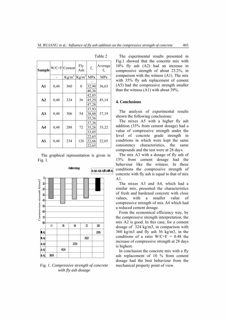
M. RUJANU et al.: Influence of fly ash addition on the compressive strength of concrete 403

Table 2

W/C+F Cement Fly Ash

fc Average

fc Sample

- Kg/m3 Kg/m3 MPa MPa -

32,90A1

0,48

360 0 40,36

36,63

42,8545,29A2 0,48 324 36 47,28

45,14

37,9338,08A3

0,48

306 54

35,5637,19

37,3635,26A4

0,48

288 72

33,0535,22

22,6522,66A5 0,48 234 126 22,65

22,65

The graphical representation is given in

Fig. 1.

Fig. 1. Compressive strength of concrete with fly ash dosage

The experimental results presented in Fig.1 showed that the concrete mix with 10% fly ash (A2) had an increase in compressive strength of about 23.2%, in comparison with the witness (A1). The mix with 35% fly ash replacement of cement (A5) had the compressive strength smaller than the witness (A1) with about 39%.

4. Conclusions

The analysis of experimental results

shown the following conclusions: The mixes A5 with a higher fly ash

addition (35% from cement dosage) had a value of compressive strength under the level of concrete grade strength in conditions in which were kept the same consistency characteristics, the same compounds and the test were at 28 days.

The mix A3 with a dosage of fly ash of 15% from cement dosage had the behaviour like the witness. In these conditions the compressive strength of concrete with fly ash is equal to that of mix A1.

The mixes A3 and A4, which had a similar mix, presented the characteristics of fresh and hardened concrete with close values, with a smaller value of compressive strength of mix A4 which had a reduced cement dosage.

From the economical efficiency way, by the compressive strength interpretation, the mix A2 is good. In this case, for a cement dosage of 324 kg/m3, in comparison with 360 kg/m3 and fly ash 36 kg/m3, in the conditions of a ratio W/C+F = 0.48 the increase of compressive strength at 28 days is highest.

In conclusion the concrete mix with a fly ash replacement of 10 % from cement dosage had the best behaviour from the mechanical property point of view.

0

10

20

30

40

50

60

70

80

Addition dosage

Com

pres

sive

stre

ngth

N/m

m2

A1 A2 A3 A4 A5

A5 22,65

A4 35,22

A3 37,19

A2 45,14

A1 36,63

0 36 54 72 126


404

References

1. Bolden J., Abu-Lebdeh T., Fini E., Utilization of recycled and waste materials in various construction applications, American Journal of Environmental Science, 9 (1) 2013, p:14-24.

2. Barbuta M, Harja M, Babor D., Concrete polymer with fly ash. Morphologic analysis based on scanning electron microscopic observations. Rev Rom Mat., 2010, 40:337–345.

3. Harja M, Barbuta M, Rusu L., Obtaining and Characterization of Polymer Concrete with Fly Ash. J Appl Sci., 2009, 9:88–91.

4. Harja M, Barbuta M., Influence of different additions on frost-thaw and chemical resistance of polymer concrete. Adv Sci Lett., 2013, 19:455–459.

5. Bărbuţă M, Harja M, Cretescu I, Soreanu G., Influence of wastes content on properties of polymer concrete. 7th International Symposium on Cement Based Materials for a Sustainable Agriculture, Canada, 2011,18-21 septembrie.

6. Magureanu C, Negrutiu C. Performance of concrete containing high volume coal fly ash - green concrete. 4th Int Conf Comp Methods Exp Mat Charact, Proc Paper 2009, 64, p: 373-79.

7. Barbuta M., Effect of different types of superplasticizer on the properties of high strength concrete incorporating large amounts of silica fume, Bullettin of the Polytechnic Institute of Iasi, construction and Architecture Section 51 (1-2), 2005, p: 69-74.

8. Sofi, J.S.J. van Deventer, P. A. Mendis, G.C. Luckey, Engineering properties of inorganic concretes, Cement and Concrete Research, 37, 2007,251-257

9. Hardjito D., Steenie E. Wallah S. E., Dody M. J. Sumajouw D. M .J., Rangan B. V. -On the Development of Fly Ash-Based Geopolymer Concrete, Materials Journal, 2004, 101,6, p: 467-472

10. Harja M, Barbuta M, Gavrilescu M., Utilization of coal fly ash from power plants II. Geopolymer obtaining. Env Eng Manag J., 2009, 8:513–520

11. Barbuta M, Harja M., Use of geopolymers for preparing concrete. Proceedings of IV-th National Conference The Academic Days of Academy of Technical Science in Romania, Iasi, 2009, 2:23-29.

12. Neville, A., H., Properties of Concrete, Longman Group Limited, London, 1997

13. Barbuta M, Harja M, Baran I., Comparison of Mechanical Properties for Polymer Concrete with Different Types of Filler. J Mater Civ Eng., 2010, 22:696–701.

14. Rujanu, M., PhD Thesis, Facultatea de Construcţii şi Arhitectură Iaşi, 1993

15. Cod de practica pentru executarea lucrarilor din beton, beton armat si beton precomprimat, Partea 1: Producerea betonului, Indicativ NE 012-1:2007, Elaborat de INCDCEC-Bucuresti

16. Bucur R. D., Cimpeanu C., Barbuta M, Ciobanu G., Paraschiv G., Harja M., A comprehensive characterization of ash from Romania thermal power plant, Journal: Food, Agriculture and Environment (JFAE),2014, Vol. 12, 2: 943-949.


SOME IMPLICATIONS OF STRONG

MOTION ACCELEROGRAMS OBTAINED IN ROMANIA

H. SANDI1 I. S. BORCIA2

Abstract: The regulatory literature concerning the earthquake protection reveals the fact that the design parameters are prescribed assuming implicitly a linear performance of the ground – structure interface. Thereafter, the upper part of the ground – structure system may be eventually designed recognizing explicitly the post-elastic performance of the upper part referred to. On the contrary, the scientific concern during recent decades has shown that non-linear interaction during strong earthquakes is frequently unavoidable and, perhaps, even beneficial for the capacity of structures to withstand strong seismic action. The data at hand reveal the fact that non-linear dynamic interaction had to occur in some cases, at least in terms of partial uplift of foundations. The implications of potential occurrence of non-linear performance of ground – structure systems lead logically to the need to revise the philosophy of regulatory documents. This requires at its turn an examination of the topology of transfer to ground of the seismic forces. Key words: soil – structure interaction, foundation uplift, transfer topology, code philosophy.

1 Romanian Academy of Technnical Sciences, e-mail: [email protected] 2 INCD URBAN-INCERC, Bucharest, Romania. e-mail: [email protected]

1. Introduction A look to the regulatory literature

concerning the earthquake protection of buildings and other structures reveals the fact that the parameters concerning the specification of design loading are routinely prescribed assuming implicitly a linear performance of the ground – structure interface (or contact system). Thereafter, the upper part of the ground – structure system may be eventually designed recognizing explicitly the post-elastic performance of the upper part referred to. In agreement with the scientific impact of the modern philosophy of the

New Zealand school on earthquake resistant design, the ground performance should be, implicitly, in a mandatory way, linear. On the contrary, the scientific concern during recent decades on ground – structure interaction (which has become feasible due to the progress of calculation capabilities), has shown that non-linear interaction during strong earthquakes is frequently unavoidable and, frequently, even beneficial for the capacity of structures to withstand strong seismic action. Note here some representative papers, [2], [3], as well as two early representative papers of Romania, [4], [1].

After some methodological




406

considerations, the data at hand on structural performance of some buildings, as revealed by simultaneous accelerograms obtained at ground and at top level, reveal the fact that non-linear dynamic interaction had to occur, at least in terms of partial uplift of foundations.

The implications of potential occurrence of non-linear performance of ground – structure systems lead logically to the need to revise the philosophy of regulatory documents. Prior to specifying the seismic loading parameters, the weak links of ground – structure systems are to be identified, and this requires at its turn an examination of the topology of transfer to ground of the seismic forces.

2. Some methodological references

The references to the case studies presented in next section make use of some methodological developments that are to be briefly recalled. They are related to:

1. Ways of characterizing the seismic motion of ground and/or structures.

2. Ways of dealing in a simplified manner with the kinematics of dynamic systems analysed.

Some brief data on these developments are presented subsequently.

2.1. Ground motion characteristics used

The basic full characterization of actual

ground motions is provided by the accelerograms recorded. Since we are interested in the spectral content as well as the destructive potential of ground motion, it is most useful to undertake some appropriate ways of processing referred to.

The most usual way to do that is to determine the response spectra for absolute or relative accelerations, velocities or displacements, depending upon the type of analysis performed. These functions refer usually to ground motions. They may be of

interest even for some locations on structures, in case one installs there some valuable and vulnerable components of equipment.

Another way of high interest to analyse the features of ground motion, as well as of motion of various objects, is represented by the Fourier spectra, (complex or absolute). This approach makes it possible to analyse in a comprehensive way the features of seismic motion of ground or other objects and to derive in a reversible way the motion characteristics of various objects of interest in one sense of passage or in the opposite sense. It is usable as far as the systems dealt with present a linear performance.

Besides the ways widely known and used referred to, it may be interesting to use also the intensity spectra [9]. This approach makes it possible to get a condensed and flexible characterization of the severity of ground motion, providing a synthetic view capable to generalize in terms that are of interest for engineering activities, of the destructive potential of ground motion, for various spectral bands and also for various directions. This approach is not used in this paper, due to overall length limitation. Details on this subject can be read in [5], [7].

2.2. Dealing with the kinematics of the

systems analysed

The systems analysed in this view are relatively tall residential buildings like those of Fig. 2. Some general data on their ambient oscillation were given in [10]. The structures dealt with are assumed to be dynamically symmetrical with respect to two (orthogonal) vertical planes (referred to as longitudinal and transversal main planes). The main components of their deformation analysed on the basis of full scale experimental results refer to the features of motion in a principal (longitudinal or transversal) vertical plane. The structures dealt with are considered vertical macro-cantilevers. The full scale

H. SANDI et al.: Some implications of strong motion accelerograms obtained in Romania

407

experimental data at hand were referred to this basic model. The types of macro-deformation of these systems are:

a) Rigid tilting (due to ground deformation);

b) Pure bending; c) Pure shear. The full scale experimental data have

shown that, for oscillations in the longitudinal plane, the pure shear contributes with around 50% of the amplitude of displacements at the top, while for oscillations in the transversal plane the contribution of tilting and or pure bending is usually more than 50%. In spite of accepting a quite crude idealization, the oscillations of these dynamic systems will be assumed to correspond purely to rigid tilting.

An exercise in dealing with the relationship between pure rigid tilting and vertical motions is presented for the simple case of a vertical macro-cantilever. The interface with the ground is a rectangle of dimensions a and b respectively and the height is h (from the centre of ground – structure interface to the top). The axes Ox and Oy have an origin located at the centre of the rectangle referred to, while the axis Oz with a coordinate (increasing upwards) corresponds to the intersection of the two main vertical planes mentioned. The (infinitesimal) rotations considered are φ (rotation from Ox to Oz) and ψ (rotation from Oy to Oz) respectively. The displacements along the axes Ox, Oy and Oz are u, v and w respectively. The angles of rotation are

φ = ∂w/∂x = - u / h (1.a) ψ = ∂w/∂ y= - v / h (1.b)

The vertical displacement at a current point of coordinates x and y (assuming no vertical displacement at the origin of axes) is

w (x, y) = φ x + ψ y (2)

The vertical displacements at the corners of the horizontal plane section are, under these assumptions,

w (± a /2, ± b / 2, t) =

= ± φ (t) a / 2 ± ψ (t) b / 2 (2’)

The equation (2’) may be used for displacements, velocities or accelerations. The time variable during the seismic event, t, was explicitly introduced just in the equation (2’), but it is self-understood that it may be introduced already in former equations. The functions characterizing the variable position of the ground structure interface during an earthquake are the vertical displacements at the four corners, w (± a /2, ± b / 2, t). Due to the dynamic symmetry assumed for the dynamic system dealt with, the order of the interface corners is not significant.

3. Some case studies

The data referred to subsequently rely on

the strong motion information at hand, obtained from the accelerographic network in operation during last decades. This network pertains to the Building Research Institute INCERC – Bucharest and consists of analog accelerographs (mainly SMA-1).

Romania was subjected during last decades to three strong Vrancea earthquakes, as shown in Table 1. While in 1977 the strong motion network of INCERC consisted of a very small number of accelerographs, the situation changed totally thereafter, mainly due to the generous aid provided in 1978 by the Agency of International Development of the State Department of USA.

Data on earthquakes referred to Table 1

No Earthquake h (km) Date 1 MGR = 7.2 109 1977.03.04 2 MGR = 7.0 133 1986.08.30 3 MGR = 6.7 91 1990.05.30


408

The strong motion network that provided records during the earthquakes referred to consists currently of analog instruments, most of them of SMA-1 type, produced by Kinemetrics (USA). The location of towns where instruments are installed is shown in Fig. 1. The results concerning the features of ground motion, obtained by the network referred to were presented and discussed in several papers, [6], etc., but less attention was paid to date to the performance of structures, as revealed by motion records obtained at the top level of several buildings. A recent publication on this subject was [8]. Since the main object of this paper is to identify some features of the non-linear performance of buildings, attention is paid to some cases concerning buildings like those of Fig. 2, subjected to some of the earthquakes mentioned in Table 1.

Fig. 1. Analogical strong motion network of Romania

The time histories of horizontal

accelerations recorded are given in Fig. 3. for some cases, if possible together for ground and top levels of a same building dealt with, for the two horizontal

directions. The Bucharest - INCERC and Bucharest – Balta Albă, data of 1977.03.04, are given together in Fig. 3.1, since accelerographic information at that date was available only for ground level at

Fig. 2.1. BUCHAREST, Balta Albă, E.5,

BLA

Fig. 2.2. BUCHAREST, Alexandria 114,

OD1 Bldg., RAH

Fig. 2.3. PLOIEȘTI – WEST, 149 C Bldg.,

PLS

Fig. 2. Buildings where non-linear performance apparently occurred during

recent earthquakes.

INCERC and top level at Balta Albă. This arbitrary latter combination was adopted because only these records were available for the event of 1977.003.03, while for other cases the accelerograms are given


409

Fig. 3.1. Accelerograms at top level of

building of Fig. 2.1. and at ground level, at INCERC, on 1977.03.04.

Fig. 3.2. Accelerograms at top and ground

levels of building of Fig. 2.3 on 1986.05.30.

Fig. 3.3. Accelerograms at top and ground

levels of building of Fig. 2.2. on 1990.05.30.

Fig. 3.4. Accelerograms at top level of building of Fig. 2.2. on 1990.05.30.

Fig. 3. Accelerogams referred to in the paper.

Fig. 4.1. Fourier spectra of accelerograms at

top level for building of Fig. 2.1, for both directions, for the event of 1977.03.04.

Fig. 4.2.a Fourier spectra of accelerograms at top level for building of Fig. 2.3, for the

longitudinal direction, for the event of 1986.08.30.

Fig. 4.2.b.Fourier spectra of accelerograms at top level for building of Fig. 2.3, for the

transversal direction, for the event of 1986.08.30.


410

Fig. 4.3. Fourier spectra of accelerograms at

top level for building of Fig. 2.2, for both directions, for the event of 1990.05.30.

Fig. 4. Fourier spectra for some buildings and events

Fig. 5.1. Vertical accelerograms derived for the corners of building of Fig. 2.1, for the

event of 1977.03.04.


event of 1986.


event of 1990.05.30.


event of 1990.05.30.

Fig. 5. Vertical accelerograms derived assuming rigid body motion for the

buildings and events referred to.

together for ground and top levels for the various cases. The accelerograms for the cases of Bucharest - INCERC and Bucharest – Balta Albă, on 1977.03.04, are given together, since accelerographic data and Fourier spectra were quite similar for other events [6].

The acceleration amplitude Fourier spectra are given in Fig. 4. It was estimated that, given the limited length of the paper, other characteristics of motion, like response spectra or intensity spectra, should not be presented here.

Some comments on the figures presented:

- The buildings dealt with are quite similar and are also representative for and important part of mass construction


411

achieved in Romania, during three decades, from about 1960 to 1990;

- Data provided by accelerograms, available and used, characterize some of the most severe cases of earthquake effects obtained to date in Romania during the strong earthquakes and locations for which recording instruments were installed. While the earthquake of 1977 was destructive, having a magnitude return period of around 50 years, the other two events referred to were severe too, but not destructive, and had return periods in the range of 10 to 30 years. This means that the Vrancea sesimogenic zone is able to generate also more severe earthquakes, during which non-linear performance of the soil and ground – structure interface should be characterized by higher uplift amplitudes and, perhaps, by severe local deformation of soil, generated by compressive stresses.

- The graphs of Fig. 3.2 reveal the well known fact that, for a given building, the amplitude of seismic accelerations at the top level are much more severe than those of ground level.

- The graphs of Fig. 4.2 reveal a similar fact, that amplitudes of oscillations at the top level of a building are much more severe than those of ground level. Moreover, they reveal the fact that the dominant periods (or frequencies) of motion at top level do not coincide with those of ground level, while a paramount influence of the dynamic characteristics may be remarked, especially for the plots of Fig. 4.2 (especially Fig. 4.2.b).

- A look at Figures 5 shows that partial, transient, uplift should have occurred during the earthquakes and at the locations considered. It is most likely that the phenomenon of non-linear soil performance should have occurred in several cases.

4. Final considerations 1. A look at literature shows that, while

about three to four decades ago, literature devoted to non-linear dynamic interaction was at its beginnings, by now the concern for non-linear dynamic ground – structure interaction during strong earthquakes has increasingly become a recognized, important, branch / component of earthquake engineering. In numerous cases, the concern for non-linear performance of ground – structure dynamic systems appears to be a key component of measures of earthquake protection of structures. Note here as representative the references [2] and [3].

2. The analysis of performance of structures in case of occurrence of phenomena of non-linear soil performance shows that there may be many situations for which the non-linearity of interaction turns out to be favorable. The non-linear performance of the interface of relatively tall buildings leads to a decrease of overturning stiffness as well as of overturning moments. A new problem is raised instead in case of relatively slender buildings: the risk of overturning of structures. This represents a problem of stability of position.

3. The concern for non-linear performance of ground – structure systems implies a need of methodological reconsiderations. In principle, the seismic design loading should no longer be prescribed assuming that it may be specified irrespective of possible non-linear ground – interaction. On the contrary, one should investigate the ground – structure interface, in order to determine weak links of the system.

4. It turns out that it would be correct and necessary to investigate the topology of ground – structure transfer of seismic effects. Moreover, in case the system dealt with includes also critical pieces of


412

equipment, the view on the topology referred to should be extended, by deciding which should be the most appropriate sequence of failure of parts of ground, structure, equipment etc. in case of overloading.

5. It is highest time to reconsider the philosophy of codes and, correspondingly, the procedures of design or of evaluation of vulnerability and risk of existing structures, adopting an appropriate methodology.

6. The problems raised by the methodological modifications required are quite complex and, in order to reach satisfactory solutions, research of analytical nature should be organized. Of course, in depth analysis of the actual performance of structures, paying special attention to instrumental information will be necessary. References

1. Constantinescu, D., Dimitriu, D.: Efecte

ale rotirii fundaţiei pe teren asupra răspunsului dinamic al structurii. Construcţii, 6, 1985.

2. Gazetas, G.: Apostolou, M.: „Nonlinear Soil–Structure Interaction: Foundation Uplifting and Soil Yielding”, Proceedings Third UJNR Workshop on Soil-Structure Interaction, March 29-30, 2004, Menlo Park, California, USA.

3. Pecker, A.: „Non-linear soil structure interaction: impact on the seismic response of structures”.Gėodynamique et structure. OECD / NEA IAGE IAEA ISCC Workshop on SSI, Ottawa, 2010.

4. Sandi, H.: “Interacţiunea dinamică dintre structură şi terenul de fundare” (Dynamic interaction between structure and soil). Construcţii, 4-5, 1985.

5. Sandi, H., Borcia, I. S.: “Intensity spectra versus response spectra. Basic concepts and applications.” Pure and Applied Geophysics, Springer, 2011, Volume 168, Numbers 1-2, Pages 261-287, ISSN 0033-4553.

6. Sandi, H., Borcia, I. S.: "A summary view of instrumental data on recent strong Vrancea earthquakes and implications for seismic hazard". Pure and Applied Geophysics, 2011, Volume 168, Numbers 3-4, Pages 659-694, ISSN 0033-4553.

7. Sandi, H., Borcia, I. S.: ”An attempt to recalibrate instrumental criteria for intensity assessmeent”. Proc. 15-th European Conference on Earthquake Engineering, Istanbul, 2014

8. Sandi, H., Borcia, I. S.: Some implications of full scale data obtained during recent strong Vrancea earthquakes on the assessment of seismic risk. Proc.Comportarea in situ a construcţiilor, Braşov, 2014

9. Sandi, H., Floricel, I.: “Some alternative instrumental measures of ground motion severity”. Proc. 11-th European Conf. on Earthquake Engineering, Paris, 1998

10. Sandi, H., Şerbănescu, Gh.: “Experimental results on the dynamic deformation of multi-story buildings”. Proc. 4-th World Conf. on Earthquake Engineering, Santiago, 1969.


CASE STUDY REGARDING EVALUATION

AND CONSOLIDATION OF BUILDINGS INFRASTRUCTURE

M. SOLONARU1 M. BUDESCU I. LUNGU 1 2

D. OANEA (FEDIUC)1

Abstract: Rehabilitation solutions in terms of increasing the footing dimensions and foundation depth can be established by correlating the present soil parameters with the new loading conditions. Following the Eurocodes provisions, the evaluation of the geotechnical conditions of the existing buildings, results in stronger restrictions than the ones of previous norms. The paper presents a case study on correlating increased footings with natural soil conditions while rehabilitation regards the entire building. Key words: geotechnical evaluation, infrastructure of buildings, soil parameters.

1 Department of Structural Mechanics, Faculty of Civil Engineering and Building Services of Iasi. 2 Department of Transportation Infrastructure and Foundations, Faculty of Civil Engineering and Building Services of Iasi.

1. Introduction The assessment of the technical

condition of existing buildings is performed when it presents a significant degree of damage due to external factors that endanger the safety of operation, when changing the beneficiary or if required by the builder structural changes, additions or disposal of storey, or changes of the destination of the building. In any of these cases, it may be necessary structural rehabilitation of the building, in order to meet the requirements of strength and stability of the existing structural assembly.

The present paper aims, through a case study, to evaluate the need for infrastructure interventions when changing the destination of the building, introducing

an additional level and retrofitting the superstructure. As a consequence of failure to fulfill resistance restrictions, strengthening solutions for shallow foundations are analyzed in order to increase the bearing capacity for taking over new loads, either by enhancing the width of the foundation, or the foundation depth or simultaneously by both.

2. Geotechnical assessment outcomes for

the building infrastructure

In this case study, the infrastructure of a building consisting of continuous foundations under the walls is subjected to analysis. In terms of original technical design, the existing infrastructure, has met safety threshold. Initial data used to assess the bearing capacity of the foundation is:


414

y checking relation [3], [

(1)

rom the most unfavorable group

/ design resistance of the foundation soil.

irement that must be fulfilled [2], [4] is:

d (2)

sign value of the resistance against a

;

d=565.194 kN – relation

Rd=565.194 kN – re

over the st

building

kN; Rd=1329 kN –

; R =866.011 kN –

R =866.011 kN – re

trengthening of the foundation is imposed.

rehabilitation of the foundation

- Permanent load, P=450 kN; - Variable load, Q=150 kN; - Width of foundation, B=3 m; - Depth of foundation, Df=1.40 m; - Characteristics for the first layer of soil

where the active zone is forming: bulk weight of the soil, γ1=18kN/m3, internal friction angle, Φ1=15˚, cohesion, c1=12kPa and the height of the layer, H1=2.90m. Thus, the bearing capacit

5] is as follows: Q m R

Where, Q – Design load on the foundation soil, derived factions; m – Coefficient for working conditions; R – Bearing capacity

( 700 .8 ) ( 72 3 .816 )k N m R k N Although safety is achieved at the level

of the footing, the superstructure presents degradations and therefore for comparison purposes, the geotechnical assessment is performed in current conditions, based on Eurocodes design rules, according to the design approach GEO as an ultimate limit state. Requ

Q

dV R Where, Vd – Design value of the vertical load or normal component of resultant of theactions applied to the base of foundation; Rd – Dection. Calculation at ultimate limit state GEO

[4] is performed based on the three design approaches that differ through applying of partial safety factors for actions, materials/ soil and resistances. Since the second design approach leads to intermediate values, for this case study, the values of the first (which has two combinations of calculation AC1C1 and AC1C2) and the

third design approaches (AC3) will be compared. The values involved for checking the relation of the bearing capacity for each design approach are: - First design approach, combination one, with the notation AC1C1: Vd=968.58 kNRd=820.774 kN – relation (2) unfulfilled. - First design approach, second combination, with the notation AC1C2: Vd=745.8 kN; R(2) unfulfilled. - Third design approach, with the notation AC3: Vd=968.58 kN;

lation (2) unfulfilled. By evaluating the infrastructure under

the current conditions, lack of safety is observed, as the criterion is not achieved in any of the design approaches. It is recommended to redo the geotechnical study, which reveals the effect in time of the compaction under load

rength parameters of the soil. The new values for the soil resistance

parameters are: Φ=18˚ and c=18kPa. The results after re-evaluating theinfrastructure are the following: AC1C1: Vd=968.58 relation (2) fulfilled; AC1C2: Vd=745.8 kN d

relation (2) fulfilled; AC3: Vd=968.58 kN; d

lation (2) unfulfilled. It is noted an increase of the resistance

design values, but not sufficient for the third design approach. Thus, taking into account the unfulfilled safety criterion under initial load conditions and the new loads that will follow from adding a storey, the change of the building destination and the rehabilitation of the superstructure, the s 3. Technical solutions for the geotechnical

Structural rehabilitation of the

M. SOLONARU et al.: A study case regarding evaluation and consolidation of buildings infrastructure 415

2kPa and the bulk

esign approach a

Figure 1 shows the effect of increasing

Fig. 1. Consolidation of the foundation by increasing the foundation width

infrastructure by increasing the width of footing is one of the most common technological methods for getting an intake of bearing capacity, although to a limited extent. The new data involved in the calculations in this phase is: the permanent load from strengthening the superstructure, Pc=200kN, permanent load by adding a storey, Ps=250kN, variable load from the change of the building destination, Qsd=50kN, and the characteristics of the second soil layer that will be included in the active area (internal friction angle, Φ2=18˚, cohesion, c2=1weight, γ2=20kN/m3). According to contribution brought through the variation of the foundation depth and the increased foundation dimensions, the ratios between the resistance values and the design values of the load transmitted to the foundation (Rd/Vd) are graphically represented for each the dccording to Eurocode 7.

the foundation width. The area above the horizontal line from the unit value level represents the safety area of the strengthened foundation fulfilled for each design approach.

It is noted that simultaneously, the three approaches only satisfy the condition of safety at a width of 5.60m, thus the use of this technical solutions in the geotechnical rehabilitation being irrational. Figure 2 shows the effect of increasing the depth of foundation. As in the previous case, the area above the horizontal line from the unit value level represents the safety area of reinforced foundation.

Looking at graph it can be observed that the safety threshold is attained simultaneously for all the three approaches for a value of 4.30m for the depth of foundation, a value that can only be justified only if the beneficiary requires that a basement should be added at the existing construction.


416

Fig. 2. Consolidation of the foundation by increasing the foundation depth

The rehabilitation solution of the foundation, both by increasing the width and depth of foundation, with the results deducted by calculation is presented below. Tables 1-3 summarize the results of the ratios between the design values of resistance and design values of the loads transmitted to the foundation per meter (Rd /Vd) for all possible combinations of the values of the foundation width (horizontal direction) and of the depth of foundation (vertical direction). The ranges for these values are of 3.20m-5.60m for the width of foundation and of 1.50m-3.60m for the foundation depth. The maximum extreme values of these structural dimensions (5.60m and 3.60m) are the first values that exceed the safety threshold in the most restrictive design approach.

In order of appearance, the tables correspond to the first design approach with the two possible combinations and to the third design approach.

The area in the tables with values fulfilling the safety criterion is separated from the ones not fulfilling it through a diagonally thicker line.

Values marked by yellow represents all the values that do not satisfy the condition of resistance for first approach, first combination; similarly, values marked with red do not satisfy the safety criterion for the second combination from the first design approach and values marked with blue do not verify the criterion for the third design approach.

The gray boxes of the tables with solid values include the first values that satisfy the condition of bearing capacity for all design approaches at the same time. The strengthening solution can be achieved by choosing any value below the thicker line, which separates the safety area and the uncertainty area, this value being corresponding to a pair of values for a width (B) and a depth of foundation (Df).

M. SOLONARU et al.: A study case regarding evaluation and consolidation of buildings infrastructure 417

DA1C1 3.2 3.4 3.6 3.8 4 4.2 4.4 4.6 4.8 5 5.2 5.4 5.6 B

Df Rd/Vd

Rd/

Vd

1.5 0.876 0.936 0.9959 1.2406 1.3025 1.3656 1.4289 1.492 1.557 1.621

1.6 0.889 0.949 1.192 1.2542 1.3166 1.3793 1.4425 1.505 1.569 1.6341.7 0.902 0.962 1.206 1.2681 1.3303 1.3929 1.4559 1.519 1.583 1.6471.8 0.914 0.974 1.219 1.2805 1.3432 1.4061 1.4687 1.532 1.596 1.6591.9 0.926 0.987 1.17 1.232 1.294 1.3565 1.4193 1.4816 1.545 1.609 1.672

2 0.938 0.999 1.183 1.245 1.3072 1.3696 1.4315 1.4943 1.56 1.62 1.6842.1 0.95 1.196 1.258 1.3197 1.3818 1.4441 1.5073 1.569 1.633 1.6962.2 0.962 1.208 1.27 1.3319 1.3945 1.4567 1.5195 1.581 1.644 1.7072.3 0.973 1.221 1.282 1.3445 1.4064 1.4688 1.5307 1.593 1.656 1.719

2.4 0.985 1.171 1.232 1.294 1.3565 1.4186 1.4809 1.543 1.606 1.667 1.732.5 0.996 1.182 1.244 1.307 1.3688 1.4301 1.4926 1.5547 1.617 1.679 1.742.6 1.194 1.256 1.318 1.3802 1.4419 1.5044 1.5661 1.628 1.69 1.7512.7 1.206 1.268 1.33 1.3916 1.4538 1.5152 1.5774 1.639 1.701 1.762

2.8 1.1542 1.217 1.279 1.341 1.4033 1.4653 1.527 1.5881 1.65 1.711 1.7732.9 1.1657 1.228 1.29 1.352 1.4144 1.4761 1.5376 1.599 1.66 1.722 1.783

3 1.465 1.555 1.645 1.73 1.822 1.91 2 2.089 2.1771 2.2659 2.354 2.442 2.53

3.1 1.479 1.57 1.6585 1.747 1.837 1.926 2.0148 2.1032 2.1918 2.2796 2.368 2.456 2.5433.2 1.493 1.583 1.6732 1.762 1.851 1.941 2.0289 2.117 2.2047 2.2932 2.381 2.467 2.5543.3 1.507 1.597 1.6868 1.777 1.865 1.954 2.0428 2.1305 2.2184 2.3054 2.393 2.48 2.5663.4 1.52 1.611 1.7003 1.79 1.879 1.968 2.056 2.1439 2.2314 2.3185 2.406 2.492 2.5783.5 1.534 1.624 1.7145 1.804 1.892 1.981 2.0695 2.1571 2.2448 2.3314 2.418 2.504 2.59

3.6 1.547 1.638 1.7276 1.818 1.906 1.995 2.0828 2.1696 2.2573 2.3441 2.43 2.516 2.601D A 1C 1

1.056 1.118 1.179

1.0088 1.07 1.1311.0222 1.083 1.1441.0348 1.096 1.1571.0472 1.109

1.0601 1.1221.011 1.0722 1.1341.023 1.0841 1.1461.035 1.0965 1.159

1.047 1.10861.058 1.1201

1.007 1.069 1.1321.018 1.081 1.1432

1.029 1.0921.04 1.103

The degree of meeting the ULS condition for the variation of B and Df according to

DA1C1 Table 1

DA1C2 3.2 3.4 3.6 3.8 4 4.2 4.4 4.6 4.8 5 5.2 5.4 5.6 B

Df Rd/Vd

Rd/

Vd

1.5 0.748 0.797 0.8465 1.047 1.0973 1.1485 1.2 1.252 1.303 1.354

1.6 0.76 0.81 1.011 1.0609 1.1114 1.1637 1.2145 1.265 1.317 1.3691.7 0.773 0.823 1.025 1.0746 1.1261 1.177 1.2287 1.28 1.332 1.3841.8 0.785 0.836 1.038 1.0889 1.1398 1.1917 1.2427 1.294 1.346 1.3971.9 0.797 0.848 1.001 1.051 1.1021 1.1533 1.2052 1.2565 1.308 1.36 1.411

2 0.809 0.86 1.013 1.065 1.116 1.1673 1.2187 1.27 1.32 1.373 1.4242.1 0.821 1.026 1.077 1.1288 1.1803 1.2318 1.2833 1.335 1.386 1.4382.2 0.832 1.039 1.09 1.1422 1.1932 1.2456 1.2963 1.347 1.399 1.452.3 0.844 1.051 1.103 1.1547 1.2065 1.2575 1.3092 1.361 1.412 1.464

2.4 0.856 1.012 1.064 1.116 1.1677 1.2189 1.2709 1.322 1.373 1.424 1.4752.5 0.867 1.024 1.076 1.128 1.1798 1.2312 1.2831 1.3342 1.386 1.437 1.4882.6 1.036 1.088 1.14 1.1916 1.244 1.2945 1.3465 1.398 1.449 1.52.7 1.048 1.1 1.152 1.2042 1.2558 1.3073 1.3585 1.41 1.461 1.511

2.8 1.0064 1.059 1.111 1.164 1.2157 1.2675 1.319 1.3703 1.422 1.473 1.5232.9 1.017 1.071 1.123 1.176 1.2278 1.2797 1.3313 1.382 1.433 1.484 1.5343 1.237 1.31 1.384 1.46 1.529 1.6 1.673 1.744 1.8154 1.8868 1.958 2.027 2.098

3.1 1.25 1.324 1.3978 1.471 1.543 1.616 1.688 1.759 1.8299 1.9008 1.971 2.041 2.1113.2 1.264 1.338 1.4123 1.485 1.558 1.629 1.7016 1.7733 1.8437 1.9145 1.985 2.055 2.1253.3 1.277 1.352 1.4256 1.498 1.571 1.643 1.7162 1.7874 1.8578 1.9287 1.998 2.068 2.1373.4 1.291 1.365 1.4388 1.512 1.585 1.657 1.7294 1.8013 1.8711 1.942 2.013 2.081 2.153.5 1.303 1.378 1.4521 1.526 1.598 1.671 1.7425 1.8144 1.8848 1.9551 2.025 2.094 2.164

3.6 1.316 1.391 1.465 1.539 1.612 1.684 1.7565 1.8279 1.8978 1.9686 2.039 2.106 2.176D A 1C 2

0.896 0.946 0.997

0.8598 0.91 0.960.873 0.923 0.9740.8853 0.937 0.9870.8988 0.95

0.9107 0.9630.872 0.9239 0.9750.884 0.9363 0.9880.896 0.9478 0.999

0.908 0.96050.919 0.9717

0.878 0.931 0.98340.889 0.942 0.995

0.9 0.9530.91 0.964


DA1C2 Table 2


418

DA3 3.2 3.4 3.6 3.8 4 4.2 4.4 4.6 4.8 5 5.2 5.4 5.6 B

Df Rd/Vd

Rd/

Vd

1.5 0.571 0.608 0.6462 0.7981 0.8367 0.8759 0.9147 0.954 0.993 1.032

1.6 0.58 0.619 0.77 0.809 0.8477 0.8866 0.9256 0.964 1.003 1.0431.7 0.59 0.628 0.781 0.8196 0.8586 0.8971 0.9363 0.975 1.014 1.0541.8 0.599 0.637 0.791 0.8296 0.8688 0.9075 0.9463 0.986 1.025 1.0641.9 0.608 0.647 0.763 0.801 0.8399 0.8788 0.9182 0.9567 0.996 1.035 1.074

2 0.617 0.656 0.772 0.811 0.85 0.8891 0.9277 0.9668 1.01 1.045 1.0842.1 0.626 0.782 0.821 0.86 0.8988 0.9376 0.9768 1.016 1.055 1.0932.2 0.635 0.792 0.831 0.8693 0.9083 0.9478 0.9866 1.025 1.064 1.1032.3 0.643 0.801 0.84 0.879 0.9182 0.9568 0.9958 1.035 1.074 1.113

2.4 0.652 0.771 0.81 0.849 0.8885 0.9274 0.9666 1.005 1.044 1.083 1.1222.5 0.661 0.779 0.819 0.859 0.8979 0.9364 0.9758 1.0146 1.054 1.092 1.1312.6 0.789 0.828 0.867 0.9067 0.9459 0.9849 1.0238 1.062 1.101 1.1392.7 0.798 0.837 0.877 0.9158 0.9551 0.9938 1.0328 1.072 1.11 1.148

2.8 0.766 0.806 0.846 0.886 0.9248 0.9638 1.003 1.0411 1.08 1.119 1.1572.9 0.7744 0.815 0.854 0.894 0.9336 0.9728 1.0117 1.0499 1.088 1.127 1.165

3 0.942 0.998 1.053 1.11 1.163 1.22 1.272 1.326 1.3794 1.4333 1.487 1.539 1.593

3.1 0.952 1.008 1.0634 1.119 1.174 1.228 1.2826 1.3364 1.3901 1.4437 1.497 1.55 1.6033.2 0.962 1.018 1.0742 1.129 1.184 1.239 1.2933 1.3469 1.4004 1.454 1.507 1.56 1.6123.3 0.972 1.028 1.0842 1.14 1.194 1.249 1.3038 1.3572 1.4107 1.4639 1.517 1.57 1.6223.4 0.982 1.038 1.0941 1.149 1.204 1.259 1.3135 1.3675 1.4207 1.4739 1.527 1.579 1.6313.5 0.991 1.048 1.104 1.16 1.214 1.27 1.3237 1.377 1.4308 1.4837 1.536 1.589 1.64

3.6 1.001 1.058 1.1137 1.17 1.225 1.279 1.3338 1.3869 1.4405 1.4938 1.546 1.598 1.65DA3

0.684 0.722 0.76

0.6557 0.694 0.7320.6661 0.704 0.7430.6754 0.714 0.7530.6851 0.724

0.6945 0.7340.665 0.704 0.7430.674 0.7133 0.7530.683 0.7224 0.761

0.692 0.73150.701 0.7399

0.669 0.709 0.74920.677 0.717 0.7574

0.685 0.7260.693 0.734


DA3 Table 3

References 4. Conclusions

The objective of this paper is to analyze the possibilities of intervention over the infrastructure of a building proposed for rehabilitation of the superstructure, the addition of a storey and the change of its destination, in order to obtain structural safety in operation and to satisfy the demands of the beneficiary.

1. Budescu, M., Țăranu, N., et al.: Building rehabilitation. Iași. Academic Publishing Society "Matei-Teiu Botez", 2003.

After the calculation analysis, increasing the width of foundation proves to be irrational through the excessive values resulted and enhancing the depth of foundation is justifiable only in case of adding a basement to the existing structure.

2. Lungu, I.: Asupra evaluării stării geotehnice a terenului de fundare de sub fundații în vederea reabilitării. In: The 12th National Conference of Geotechnical and Foundations, Stanciu et al., Politehnium Publishing House, 2012, p. 721-726.

3. Stanciu, A., Lungu, I.: Fundații (Foundations). București. Technical Publishing House, 2006.

The optimal solution recommends enhancing both the width and the depth of the foundation. The third design approach dictates the strengthening solution, being the most restrictive in the case study.

4. *** SR EN 1997-1-2004: Geotechnical design – Part 1: General rules. Accessed: 09.09.2014.

5. *** STAS 3300/2-1985: Geotechnical design – Part 1: General rules. Accessed: 09.09.2014.


TOWARDS THE INFLUENCE OF THE LOCAL COLLAPSE OF STRUCTURAL

ELEMENTS TO GENERATE PROGRESSIVE COLLAPSE

D. STOICA1

Abstract: After the total or partial collapse of several important buildings the specialists in civil engineering began to treat more seriously and accuracy the problem of completely avoiding progressive or general collapse or just in the first instance in order to ensure complete evacuation of people and / or important goods. Considering these aspects, in this paper I’ll present two parallel study cases for buildings with 5 and 10 levels, which is supposed to have a local collapse of one first floor column (corner, marginal or central) realizing simple or complex analysis in order to identify problems that ascend on the whole building. Key words: collapse; local; progressive; ductility; hinges

1 Buildings Department, UTCB – Technical University of Civil Engineering of Bucharest

1. Introduction The main objective of these studies was the assessment of influence of local/partial collapse to generate progressive collapse. In this consideration all the evaluations were performed according to the following parameters: The number of levels of structure: two

identical structures were selected with two different height levels: a low-rise structure (with 5 levels) and a medium high-rise structure (with 10 levels).

The structural damage cases: according to emergency scenarios from GSA (General Service Administration – October 24, 2013): were removed separately, one corner column, one marginal column closer to the midpoint of the structure and one of

the central columns located as close to the center of the structure.

Adopted analysis methods: usual static linear calculations were performed, followed by nonlinear static analysis (pushover) for a better interpretation of phenomena.

The secondary objective was to determine the worst damage scenario. The following steps have been completed in order to accomplish analysis: Evaluation of structural composition,

materials and loads to be taken into account;

A pre-design of all the structural elements;

Determining the status of sectional efforts and deformations using ETABS program;


420

Designing the stiffness through the lateral forces by checking the Serviceability Limit State (SLS) and Ultimate Limit State (ULS) according to Eurocode 8 (EC8);

Designing all the reinforcement types in beams and columns;

Choosing the scenarios generating local collapse under GSA recommendations in the field;

Checking the drifts for the damaged structures;

Beams behavior analysis after the columns collapse in agreement with the chosen scenarios;

Performing pushover nonlinear static analysis that followed the steps of: defining the potential plastic hinges for beams and columns; defining the load cases for nonlinear analysis; calculation of target movement according EC8.

Due to a better understanding of the structural behavior of materials and with increasing the computational power, the modern structures are better designed than in the past. This optimization resulted in the reduction of inherent safety margins, but still due to this the capacity to resist for unexpected events decreased. This increased vulnerability may be associated with modern construction methods targeting at reducing the costs and also because of the modern architectural design directions with lightweight construction and large spans. Lastly, the increased fear for terrorist threats highlighted the need to consider the design of unforeseen events such as: blasts, external impact, detonations, etc.

2. Computation Strategies The buildings studied have RC frame structure, occupying an area plan with dimensions 25x25 m2, with five spans and

five bays of 5 m. The height of 3m is set for all the levels. The building functionality were set as offices. Exterior curtain walls and interior drywall partitions were used. The concrete slabs have a thickness of 13 cm, ensuring the required strength and acoustic comfort. The buildings location were set in a region with a horizontal design acceleration (ag) of 0.30g, according to EC8. The importance and exposure class is II (γe,І = 1.0). The periods TB=0.16 sec, Tc=1.60 sec and the ductility class was set at high class (HD). The snow zone: = 2,0 kN/mkos ,

2.

Execution technology: monolithic RC (including floors).

Fig.1. Axes sketch

Used materials:

Concrete characteristics Table 1

Concrete N/mm2 N/mm2

N/mm2 N/mm2

GPa

C25/30 25 33 2.6 1.8 31 C35/45 35 43 3.2 2.2 34

Steel Characteristics Table 2

Steel N/mm2

N/mm2

N/mm2

S500 500 550 2.1E+8

D. STOICA: Towards The Influence Of The Local Collapse Of Structural Elements To Generate Progressive Collapse

421

Seismic load it was considered

defining the design spectrum:

(1)

and if (2)

As can be seen the design spectrum is obtained from the elastic spectrum by reducing the range of it with the behavior factor q for values of the period T> TB.

For periods T ≤ TB design spectrum is determined by a behavior factor q, q = 1 it reaching T = 0.

Fig.2. Comparison between elastic spectrum (red) and design spectrum

(dark blue) q= 4.73 and T= 1.6s

To determine the structural elements efforts of the building, the structural analysis program ETABS [15] were used. Dimensions obtained from the pre-design stage defined the structural elements in the program: beams and columns as linear FRAME finite elements and the slabs as planar SLAB finite elements. It was considered that concrete were cracked: for beams and for columns .

Fig. 3. Structural model in ETABS: a) 5 levels, b) ten levels

3. Scenarios That Generate Local

Collapse

The scenarios presented in this paper on the removal of the columns from the ground floor are confirmed with the recommendations of the GSA [5].

This design guide has the following structural failures: removal of a corner column; removal of a marginal column located at midpoint; removal of a central column.

Fig. 4. Structural damage types applied

to models


422

Fig. 5. Initial 5 stories structure drifts

Fig.6. 5 levels scenario cases SLS drifts

Fig.7. 5 levels scenario cases ULS drifts These cases are in accordance with the

below scenarios:

a)

b)

Fig. 8. ETABS model – removed: a) corner column; b) central/marginal

column

Fig. 9. Initial 10 stories structure drifts


423

Fig.10. 10 levels scenario cases SLS drifts

Fig.11. 10 levels scenario cases ULS drifts These cases are in accordance with the below scenarios:

Fig. 12. a) ETABS model – removed corner column

Fig. 12. b) ETABS model – removed central/marginal column

Joints deflection above the Table 3 removed columns

Joint deflection 5

levels 10 levels

Above the removal corner

column

1.25 cm

0.91 cm

Above the removal marginal column

1.13 cm

0.62 cm

Above the removal central

column

0.68 cm

0.32 cm

Beams deflection Table 4

5 levels 10 levels Deflection Removed corner column

f= 12.6mm 8.0mm

fadm= 12.5mm

f = fadm OK 12.5mm

f < fadm OK

Removed marginal column f= 12.9mm 7.2mm

fadm= 12.5mm

f > fadm Not OK

12.5mm

f < fadm OK

Removed central column f= 10.7mm 8.2mm

fadm

= 12.5mm

f < fadm OK 12.5mm

f < fadm OK


424

From all the analysis did, in the paper some synthetic and simple tables are presented in the followings: The 5 levels case:

Beams bending moments check Table 5 in case of corner column

M

Envelope Case of a corner column

failure

Levels MEd < MRd

Support 1

MEd < MRd

Support 2

MEd < MRd Mid field

1-3 OK Not OK Not OK

4-5 OK Not OK OK Gravitational

Case of a corner column failure

Levels MEd < MRd

Support 1

MEd < MRd

Support 2

MEd < MRd Mid field

1-3 Not OK Not OK OK

4-5 Not OK Not OK OK

Beams bending moments check Table 6 in case of marginal column

M

Envelope - Case of a marginal

column failure Level

s MEd < MRd

Support 1

MEd < MRd

Support 2

MEd < MRd Mid field

1-3 OK Not OK Not OK 4-5 Not OK Not OK Not OK

Gravitational - Case of a marginal column failure

Levels

MEd < MRd

Support 1

MEd < MRd

Support 2

MEd < MRd Mid field

1-3 Not OK Not OK Not OK 4-5 Not OK Not OK Not OK


M

Envelope - Case of a central

column failure Levels MEd <

MRd Support 1

MEd < MRd

Support 2

MEd < MRd

Mid field1-3 OK OK Not OK 4-5 OK Not OK OK


425

Gravitational - Case of a central column failure

Levels

MEd < MRd

Support 1

MEd < MRd

Support 2

MEd < MRd Mid field

1-3 Not OK Not OK Not OK 4-5 Not OK Not OK OK

The 10 levels case: Beams bending moments check Table 8 in case of corner column

M

Envelope - Case of a corner column failure

Levels MEd < MRd

Support1

MEd < MRd

Support2

MEd < MRd

Midfield

10 OK Not OK Not OK 8-9 OK Not OK Not OK 6-7 OK OK OK 2-5 OK OK OK 1 OK Not OK Not OK

Gravitational - Case of a corner column failure

Levels MEd < MRd

Support 1

MEd < MRd

Support 2

MEd < MRd Mid field

10 Not OK Not OK OK 8-9 OK OK OK 6-7 OK OK OK 2-5 OK OK OK 1 OK OK OK


M

Envelope - Case of a marginal column failure

Levels

MEd < MRd

Support1

MEd < MRd

Support2

MEd < MRd

Midfield

10 OK Not OK Not OK 8-9 OK Not OK Not OK 6-7 OK Not OK Not OK 2-5 OK Not OK Not OK 1 OK Not OK OK

Gravitational - Case of a marginal column failure

Levels

MEd < MRd

Support1

MEd < MRd

Support2

MEd < MRd

Midfield



426


M

Envelope - Case of a central column failure

Levels

MEd < MRd

Support1

MEd < MRd

Support2

MEd < MRd

Midfield

10 OK Not OK OK 8-9 OK Not OK OK 6-7 OK Not OK Not OK 2-5 OK Not OK OK 1 OK Not OK OK

Gravitational - Case of a central column failure

Levels

MEd < MRd

Support1

MEd < MRd

Support2

MEd < MRd

Midfield


Nonlinear static analysis (pushover)

was chosen to perform in good condition for RC frame structures in ETABS [15].

This analysis involves the gradual annoyance of displacements on the structure until it forms a plastic mechanism. As it grow the structural displacements as gradually develops plastic hinges. Plastic hinges used are of two types: beams plastic hinges (joints bending moment M3) and columns plastic hinges (joints M3 bending moment and axial force P), defined at both ends of elements. To define the performance ranges the plastic hinges rotations were definite based on the requirements of FEMA 273. For columns plastic hinges the moment-axial force interaction curve must be defined and will be introduced by points. The push-over analysis involves two assumptions: a situation where the structure is loaded by gravity load; a situation where the structure is progressively loaded horizontally. This hypothesis run after the first one. The maximum number of steps and the number of null steps are the parameters which control the run time. Reaching the maximum number of steps or null steps the analysis stops. The meaning of null steps is that a plastic hinge yield and determined the yielding of other plastic hinges. 4. Nonlinear Static Analysis Responses Interpretation The initial unaffected structures - Following the analysis it was found that: Structures were properly conformed

because the plastic hinges occurs first at the beams edges and then at the columns bases;

Until the target displacement is reach there are not occurred plastic hinges to compromise the safety of the buildings (the most requested items arrive to stage LS = Life Safety).

The structures develop plastic hinges for C – collapse stage for not much larger


427

displacement than the target displacements.

The analysis of the three scenarios for generating local collapse (removing the corner, marginal and central columns) is justified. Just several steps of each case are shown in this paper.

Plastic hinges occurrence for Table 11 the initial structures

5 levels 10 levels

Step 5

Step 7

Step 6

Step 8

Step 9 Step 7

The case of removed central column - Following the analysis it was found that: At the column base (the column above

the removed column) plastic hinge

occurs from the first step (step 2 d = 0.024 m);

At the beams above the removed column plastic hinges occurs corresponding to stage LS-CP (Life Safety-Collapse Prevention) before reaching the target displacement;

If the beams reach near the limit of CP or exceed, the structure is likely to have a progressive collapse;

Once reaching the target displacement in the beam above the removed column C plastic hinges occurs corresponding to collapse stage.

Plastic hinges occurrence for Table 12 removed central column case

5 levels 10 levels

Step 5

Step 6

Step 7

Step 8

Step 8


428

The case of removed corner column - Following the analysis it was found that: Structure behaves properly until the

target displacement, the most requested structural elements arrive to stage LS = Life Safety;

After exceeding the target displacement next item to be damaged is the marginal (central) column, as can be seen in step 9 where d = 0.175 m, at the column base and a C-collapse plastic hinge occur.

Plastic hinges occurrence for Table 13 removed corner column case

5 levels 10 levels

Step 6

Step 8

Step 6

Step 9

Step 8

The case of removed marginal column - Following the analysis it was found that: As well as the disposal of the center

column at the base of the column above the column removed the plastic hinge occurs (step 2 with d = 0.024 m);

In the beams above the removed column plastic hinges occurs corresponding to LS-CP stage (Life Safety-Collapse Prevention) before reaching the target displacement;

Plastic hinges occurrence for Table 14 removed marginal column case

5 levels 10 levels

Step 6

Step 7

collapse

Step 7

Step 8

Step 9


429

In step 7 d = 0.144 m <dt = 0.145 m, at the beam above the removed column plastic hinges occurs to C - collapse stage. Immediately in the next step, this beam and the one above it reaches point D (section suffered major irreversible degradation and retains only a residual strength);

Compared to the situations described above (removing the corner column and removing central column), the case where the marginal column is damaged is the worst.

5. Final Considerations The linear and nonlinear static analysis

found that higher structure (10 levels) has a better behavior in all three studied damage scenarios than the lower one (5 levels).

After removing the columns a redistribution of moments in the beams, adjacent to removed columns, were observed. The tensile fiber is reversed in these elements so that when the mid span bottom bending moments becomes larger and (in many cases) exceeds the bending moment capacity of the section. The mode of failure was characterized by splitting the bottom longitudinal reinforcement.

In the case of marginal removed column the level relative displacements are larger and are no longer in accordance within the allowable values prescribed by codes.

The joints above the removed columns have smaller displacement for 10 levels building than those with lower height (5 levels).

After removing the columns on the ground floor, the beams deflections

fall within acceptable limits (f≤ fadm=0.0125 m), aside from the case of marginal column removal at 5 levels building.

Nonlinear static analysis (pushover) allows to have a clearer picture of the behavior of structures.

Analyzing the damaged structures by comparison, for 5 levels building, it can be seen that when the corner column is removed, the structure has a behavior similar to the original (undamaged). The problems start to occur when eliminating marginal column because in the beams above it plastic hinges occurs suitable to stage C - Collapse before reaching the displacement target. In addition, in the column above the one removed several plastic hinges occurs which reach up to the stage LS = Life Safety.

Structures with 10 levels have a better behavior, but also removing the marginal column is the worst case (similar with the 5 levels structure).

References 1. Kokot, S and Solomos, G. Progressive

collapse risk analysis: literature survey, relevant construction standards and guidelines, European Laboratory for Structural Assessment, 2012. ISBN 978-92-79-27734-4.

2. Smith, M. Progressive Collapse Assessment-Non-linear behavior of concrete structures in damaged state, Master Thesis, 2007.

3. (NIST)., U.S. National Institute of Standards and Technology. Best Practices for Reducing the Potential for Progressive Collapse in Buildings,


430

Technology Administration, U.S. Department of Commerce, 2007.

4. EN 1990. Eurocode 0 - EN 1990: Basis of structural design. 2002.

5. Guidelines. GSA. GSA Progressive Collapse Analysis and Design Guidelines for New Federal Office Buildings and Major Modernizations Projects, General Services Administration (GSA), 2003.

6. ASCE. ASCE 7: Minimum design loads for buildings and other structures, American Society of Civil Engineers, 2005.

7. National Building Code of Canada. 8. Burnett, E.P. The avoidance of

progressive collapse: Regulatory approaches to the problem. 1975.

9. Elingwood, B.R and Dusenberry, D.O. Building Design for abnormal loads and progressive collapse, Computer Aided Civil and Infrastructure Engineering, 2005.

10. Starossek, U. Typology of progressive collapse, Engineering Structures, 2007, Vol. 29.

11. STO – 008 – 02495342 –2009 Prevention of progressive collapse of

reinforced concrete monolithic structures of buildings. 2009.

12. Kaewkulchai, G. and Williamson, E. B Beam Element Formulation and Solution Procedure for Dynamic Progressive Collapse Analysis, Computers & Structures, 2004, Vol. 82.

13. Sasani, M., Bazan, M., and Sagiroglu, S Experimental and Analytical. s.l.: Structural Journal, American Concrete Institute, 2007, Vol. 104.

14. Sadek, F., Main, J.A., Lew, H.S., Robert, S. D., Chiarito, V, El-Tawil, S. An experimental and analytical study of steel moment connections under a column removal scenario, NIST Technical Note 1669, 2010.

15. CSI. ETABS Nonlinear V 9.7.4-User manual.

16. Europe, Star Seismic. Design check of BRBF system according to Eurocode 8: Use of pushover analysis, www.starseismic.eu.

17. Sagiroglu, S. Analytical and experimental evaluation of progressive collapse resistance of reinforced concrete structures, Thessis, Northeastern University, 2012.

http://www.starseismic.eu/


A CONCEPT FOR USING RECYCLED

RUBBER GRANULES IN NOISE REDUCTION CONCRETE’S PANELS

R.G. ŢARAN1 M. BUDESCU D. COVATARIU1 1

Abstract: In traffic areas, from the outskirts of residences, systems for noise attenuation (induced by auto vehicles and trains) are necessary. Because these panels serve mostly the urban environment, its must have aesthetic aspect but in the same time must have to be easy to mount and to auto sustain themselves. Replacing the natural aggregates with recycled rubber granules it result a rubberized plain concrete used mostly in non-structural constructions. Reuse of rubber from used tyres can help prevent environmental pollution and, at the same time, contribute to building developments with lower costs. The concrete with recycled rubber has an energy absorption capacity proportionally increased. Deformation and energy absorption increases with the dimension of the rubber particle. This paper proposes manufacturing of new protective panels systems made only from concrete with recycled rubber particles. Key words: sound absorbent panels, recycled rubber, panels from concrete with recycled rubber.

1 Faculty of Civil Engineering and Building Services, “Gheorghe Asachi” Technical University of Iaşi

1. Introduction In general the construction materials

have low absorbent capacity. The curtains and other textiles, furniture even people have a contribution at the total quantity of absorption. Together they form the natural absorption, which is not enough. This manner it shows up the need to use special conceived performant absorbents.

The perceived sounds are made from two components:

1) the direct sound – the sound that propagates directly towards the ear from the origin point;

2) the indirect sound – the sound that arrives to the ear after it was reflected once or many times by certain surfaces.

When the sound collides on the surface of a material, a part of its energy is absorbed, a part is transmitted and the rest is reflected back. The surfaces with common tough finishes, like dry plaster, wet plaster, concrete and glass absorbs very little sound. Sound-absorbent materials are designed such that it absorbs a percentage of the incidence energy of the sound. Therefore, the function of a sound-absorbent material is to reduce the reflected sound, and the degree we want this depends, mainly, on the area.

Absorption mechanisms

The noise absorption represents the transformation of the kinetic energy of the


sound waves in thermic energy. A small part from a sound wave with high frequency is absorbed by the air.

The natural absorption is not enough to create an acoustic confort imposed by the norms. There are two manners to absorb the sound waves: Porous absorption and resonance.

1.1. The importance of materials for

insulation When it is considered to adopt a solution

for insulation, the choosing of the materials for insulation to be used has a very important role. Previously, it is necessary an evaluation of the noise generating source and, taking into account the results, it must be choosen those materials with the acoustic and technical properties which satisfy the insulation requirements for the source. Depending on the requirements, the insulation and sound-absorbing materials can be used as such but they can be used also as components for sandwich panels, panels that can be jointed to realise the noise barriers.

Soundproofing panels from the sound barrier structure are designed according to the characteristics of the noise sources and the characteristics of location of area, the traffic being an important element that must be considered when design a sound barrier.

Equally important as the insulation materials are the fixture. For the best results it is proper that at the assembling of

some soundproofing walls or of a floating floor, to use special vibration proof systems for each type of structure.

It is ideal that when the insulation materials are chosen, besides the acoustic performances, to give importance also to the following aspects:

- the durability of the material/of the panel in time;

- impact strength; - maintenance needs; - fireproof properties; - aggressive meteorological factors

proof; - mounting means. Due to these multiple properties, to the

importance and according to the destination area, the material gets different aspects. It has performing different functions, has the capacity to reflect the light, are resistant against fire propagation, is durable and easy maintenance.

Therefore, today there is a big range of sound-absorbent materials and structures, with multiple shapes, adequate to different requirements from an architectural project for zones with the most various destinations.

2. Acoustic and Soundabsorbing Panels

Acoustic and sound-absorbing panels can be mounted on the side of the roads, highways or railroads, near factories with noisy productive activity or in industrial areas.

Acoustic materials: Fibres (absorb high frequencies)

Panels (absorb average frequencies)

R.G. ȚARAN et al.: A Concept for using Recycled Rubber Granules in Noise Reduction Concrete’s Panels

433

Resonators (absorb adjustable frequencies)

Smooth surface (reflect sounds)

Sound-absorbing panels, besides

insulation, have high impact strength (extremely important in case of access routes delimitation for roads and railroads), no maintenance required and does not permit fire propagation (having fireproof properties), can be positioned on bridges and walkways.

Fig. 1. Model of a sound absorbent panel

Sound absorbing panels from concrete with rubber are highly resistant to extreme atmospheric conditions, both at very low temperatures, and very high temperatures, without damages.

At the moment there are a lot of areas affected by the noise pollution. Urban zones crossed by railways, areas close by depots have to be soundproofed, because the moving trains, especially at the passing over the switches, generate a very high noise pollution.

Also, the construction of some

underground or aboveground passages in cities and highways constructions makes it necessary to use some sound-absorbing panels to protect the population. 2.1. Shape optimization of acoustic

barriers

The conducted researches from all over the world leaded to the identification of numerous shapes of barriers that are much better than the usual barriers, made from a single panel with small thickness, flat and reflective. Due to the shape improvement, on a height of 2 m, it can be obtained a noise reduction, caused by the traffic, between 1.5 – 3.5 dB. We distinguish two different types of panels:

• acoustic barriers with a single reflecting edge of different shapes;

• acoustic barriers with multiple reflecting edges.

From acoustic barriers with a single reflecting edge we can remember the T or Y shape barriers, barriers with arrow-shape profile, feather, etc. In all these cases, the height of barrier and the type of the terrain on which they are placed must to be considered for the efficiency of the barriers. Also between the strong reflecting barriers, the ones with vertical faces offers better performances than the ones with slightly inclined sides.


Fig. 2. Models of enhanced acoustic barriers T profile barriers provides a substantially

improvement to the insertion loss coefficient compared to the plane reflective barriers. Nevertheless, a barrier with arrow-shape profile has a bigger

silencing coefficient than the T profile

barriers. Also, in the case of acoustic barriers with feather shape it is noticed that this silencing coefficient varies according to the tilt angle of the feather shape profile span.

Fig. 3. The diffraction phenomenon of sound waves

Fig. 4. Proposed models for acoustic barriers made from rubberized concrete

R.G. ȚARAN et al.: A Concept for using Recycled Rubber Granules in Noise Reduction Concrete’s Panels

435

Fig. 5. Acoustic barrier panels existent type

3. Soundabsorbent Panels made from

Concrete with Recycled Rubber Rubber aggregates, provided from

recycling and tyres soling, has granules of different dimensions or fibbers. Usually, the remaking is made mechanically at normal temperatures; there is another method, the remaking at very low temperatures. The remaking at normal temperatures is made by grinding the used tire or using granulation techniques. Processing at normal temperatures is done by used tires grinding or using granulation techniques.

Fig.6 Particles having different dimensions

3.1. Impact of using recycled rubber as partial replaced aggregate in concrete was well documented by compression tests, traction and bending

The maximum rubber aggregate quantity

that can be replaced must be determined, although previews studies shown that in fresh state as well as in harden state, the ideal quantity of aggregate with the dimension under 4 mm has to be maxim 180 kg/m3 (max 15%).

Rubber aggregate maximum quantity that can be replaced must be measured in such a way that the concrete have a homogeneous structure.

Maximum recycled rubber admixture from the concrete mix must not exceed 75 % so that the aggregate to be integrated into the mix.

Fig.7 Sound-absorbing panel from concrete with rubber particles

The deformation and energy absorbing

capacity increased with the increasing of rubber sizes when the rubber contents remained constant (increasing the granule’s dimensions tends to increase the energy’s adsorption). It results that the impact energy of the rubber based concrete panels is bigger comparing to energy impact from plain concrete panels, fact that


leads to survival chances increases in case of a collision of a vehicle with the panel.

Fig.8 Detail of the concrete’s structure with rubber particles

Main disadvantages as follows (shading, low light transmission, bad visibility of the drivers from streets, roads and highways) must be compared from the other aspects. The impact strength is also an extremely important characteristic, in case of a collision of a vehicle with the soundproofing wall, the panel being built

from concrete. 4. Final Remarks

Although the properties that are referring

to strength and durability of the concrete with recycled rubber aggregates are not favourable, this one could present some advantages. These advantages are resulted from favourable attenuation characteristics, good thermal and sound insulation of the concrete. Rubber aggregates decrease the specific weight of the mix having a larger quantity of entrapped air that makes the pumping easier.

So much more, there must be underlines the eccologically advantages brought by the recycling of the used tires that, is well known, have a low degree of natural neutralisation. Further studies are necesarry, to establish the optimum quantity of rubber aggregates in concrete and to introduce it in the actual standards and procedures. References

1. Feng Liu, Guixuan Chen, Lijuan Li,

Yongchan Guo., Study of impact performance of rubber reinforced concrete, Construction and Building Materials, China, 2012.

2. Țaran Rareș-George, Studiu referitor la proprietățile stucturilor din beton armat utilizand cauciuc reciclat, Creaţii universitare 2013, vol. 6, 2013.

3. Topçu IB, Bilir T., Experimental investigation of some fresh and hardened properties of rubberized self-compacting concrete, Mater Des 2009;30(8):3056–65

4. http://www.agir.ro/buletine/957.pdf 5. http://www.creeaza.com/tehnologie/ele

ctronica-electricitate/Realizarea-hartilor-de-zgomot515.php

7INTERNATIONAL SCIENTIFIC CONFERENCE CIBV 2014 7-8 November 2014, Braşov

SEISMIC STRENGTHENING OF A

PRECAST REINFORCED CONCRETE WALL PANEL USING NSM-CFRP

C. TODUT1 V. STOIAN D. DAN T. NAGY-GYORGY1 1 1

Abstract: The precast reinforced concrete wall panel (PRCWP) presented in this paper is part of an experimental program in which the seismic performance, weakening effects due to cut-outs, strengthening strategies and cost evaluations were investigated. The experimental specimens were 1:1.2 scaled RC as-built solid walls or as-built walls with window or door openings. The specimens were subjected to cyclic load reversals, displacement controlled. Most of the specimens were first tested unstrengthened, then after they were repaired, strengthened using FRPs and tested again. The wall panel presented here was post-damage strengthened using near surface mounted (NSM) carbon fibre reinforced polymers (CFRP). The repair and strengthening strategy steps will be presented together with the experimental results of both the unstrengthened and the post-damage strengthened specimen. Key words: seismic, strengthening strategy, RC wall, NSM-CFRP.

1 Politehnica University of Timisoara, 2nd T. Lalescu, 300223, Romania

1. Introduction The use of large panel structures was

widely used in seismic areas, because the system composed of precast reinforced concrete panels can provide an efficient performance under earthquake conditions. After 50 years of existence, which most of them have and interventions some of them were subjected to, detailed investigation is needed. The analysed specimens meet the requirements of Eurocode 8 for walls designed to medium ductility and are referred as large lightly reinforced walls.

The application of NSM-CFRP was investigated in this paper as a retrofitting strategy, in order to increase the load bearing capacity of the specimen first tested in the unstrengthened condition.

Research on NSM-FRPs studies were conducted by Sas [1], Konthesingha [2], Lee and Cheng [3], Sakar et al. [4], Stoian et al. [5], Florut et al. [6] and others.

2. Experimental Program

The experimental specimen was a 1:1.2 scaled element, namely precast reinforced concrete wall panel: PRCWP (12), designed and casted according to a Romanian Project Type 770-81 [7], [8]. PRCWP (12) specimen has an initial narrow door opening. Based on the two experimental tests performed in the unstrengthened condition and post-damage strengthened condition, important aspects related to the seismic efficiency of the strengthening system can be drawn out.


438

The experimental specimen was: 2150 mm height, 2750 mm width and 100 mm in thickness. The narrow door opening was 1800 mm height and 750 mm length. The experimental specimen was set between two reinforced steel concrete composite beams, namely a top - loading beam and a bottom - foundation beam. The web panel reinforcement of the PRCWP (12) consisted of horizontal rebars, vertical bars, welded wire mesh in the right pier, a spatial reinforcement cage on the entire height of the left pier, a spatial reinforcement cage in the coupling beam, vertical bars in the coupling beam, spatial reinforcement cage at the top right corner of the door opening, and two inclined bars at the top corners of the opening. The configuration of the experimental specimen selected for investigation is presented in Fig. 1 [11].

2.1. Material Considerations

The specimen’s concrete quality was

C25/30 class, while the reinforcement S255 was used for the spatial reinforcement cage, S355 for horizontal, vertical and inclined steel bars, and S490 for the steel wire mesh. The steel reinforcement properties obtained expe-

Fig. 1. Specimen outline and reinforcement rimentally were given in [9, 10]. Near surface

mounted CFRP plates were used for the retrofitting of the specimen. Also, carbon fibre (CF) fabric, applied externally bonded was used to improve the confinement capacity of the specimen. Table 1 summarizes the geometrical and mechanical properties of the CFRP plates and CF fabric used. The mentioned characteristics are based on manufacturer’s data. The mortar, used to replace the heavily damaged concrete was Mapegrout Easy Flow GF, having a compressive strength of 60 N/mm2 at 28 days according to the product data sheet.

2.2. Testing Methodology and Test Set-

up Detailed data related to the tests set up

and testing methodology of the precast reinforced concrete wall panel specimens were presented by Demeter [10]. A general view of the test set-up of the specimens is presented in Fig. 2.

The specimen was tested under quasi-static reversed cyclic lateral loads, displacement controlled (with two cycles per drift), of measure 0.1% drift ratio, namely 2.15 mm. Vertical loads were also applied in order to impose the gravity loading condition and to restrain the rotation of the element.

The experimental specimen was monitored during the experimental tests using pressure transducers (P), displacement transducers (D) and strain gauges applied on steel rebars, CFRP plates and CF fabric (G).

Fig. 2. General view of the test set-up CF fabric and plate properties

C. TODUT et al.: Seismic Strengthening Of A Precast Reinforced Concrete Wall Panel Using Nsm-Cfrp

439

Table1

carbon fibre fabric carbon fibre plate

0,166 1,4

300 225 g/ml4830 3100230 1702,0 2,0

Thickness [mm]

Areal weight [g/m2]Tensile strength [MPa]Tensile modulus [GPa]Elongation at break [%]

Component

Product name MapeWrap C UNI-AX

Carboplate E170/100/1.4

3. Repair and Strengthening of the Specimen

The retrofitting strategy adopted here

intended to increase the initial load bearing capacity of the element, the solution being qualitative and based on the behaviour of the reference specimen.

The damaged specimen was first repaired by removing the crushed concrete and replacing it with a high-strength repair mortar (Fig. 3a). The wall surface was then polished locally with a special grinder (Fig. 3b) to achieve a fully smooth surface for the externally bonding application, channels were cut for the CF plates (Fig. 3c), and the concrete edges of the element were rounded at a radius of approximately 20 mm to achieve the effectiveness of the confining solution. Local holes were drilled in the panel to provide the anchors for the confinement strengthening system (Fig. 3d), and the surface of the wall was vacuum-cleaned (Fig. 3e). The cracks were cleaned and filled superficially with epoxy resin.

According to the strengthening strategy, the NSM plates (Fig. 3f) (10 mm x 1.4 mm) were mounted horizontally in the piers and in the spandrel in each side of the wall at 200 mm centres (Fig. 3g). All CF plates were anchored in the wing element. CF confinement strips (Fig. 3h) were applied at the corners of the door opening and vertical, wrapping from one face to the other of the spandrel, and at the ends of the wing walls. The completed retrofitting is shown in Fig. 3i and 3j. Fig. (3k) shows the strain gauge position on FRP plates and fabric.

a)

b)

c)

d)


440

e) i)

f) j)

g) k)

h) l)

C. TODUT et al.: Seismic Strengthening Of A Precast Reinforced Concrete Wall Panel Using Nsm-Cfrp

441

Fig. 3. The strengthening strategy

The failure of the post-damage strengthened specimen is presented in Fig. 3l, 3m and 3n. 3. Experimental Results During the experimental test of the post-damage strengthened specimen, namely PRCWP (12-E1-T/R), diagonal cracks appeared in the piers (Fig. 3l). Unfortunately, due to the capacity of the available testing facility, the specimen could not be taken to failure. The behaviour of the tested wall panel is shown in Fig. 4 as load-drift ratio response. The load bearing capacity results show a variation of 46.5 % in the positive loading cycles and 154 % in the negative loading cycles. It is obvious that the retrofitted element, namely PRCWP (12-E1-T/R) behaved highly superior compared to the reference one, PRCWP (12-E1-T).

-1000

-800

-600

-400

-200

0

200

400

600

800

1000

-0,9 -0,7 -0,5 -0,3 -0,1 0,1 0,3 0,5 0,7 0,9

[kN]

PRCWP (12-E1-T)

[%]

m) - unstrengthened specimen

-1000

-800

-600

-400

-200

0

200

400

600

800

1000

-0,9 -0,7 -0,5 -0,3 -0,1 0,1 0,3 0,5 0,7 0,9

[kN]

PRCWP (12-E1-T/R)

[%]

- strengthened specimen n)

Fig. 4. Load-drift ratio response

3. Conclusions The load bearing capacity of the specimen was increased through the retrofitting strategy, as confirmed by the load-drift ratio response of them. NSM-CFRP system can be an effective solution for strengthening elements. Further studies focused on numerical analysis, strengthening systems, openings in walls are in progress. The studies aims to establish the seismic performance of PRCWP under different parameters. Acknowledgements

The authors acknowledge the following research grant for the support of this study:

1. Grant no. 3-002/2011, INSPIRE – Integrated Strategies and Policy Instruments for Retrofitting buildings to reduce primary energy use and GHG emissions, Project type


442

PN II ERA NET, financed by the Executive Agency for Higher Education, Research, Development and Innovation Funding (UEFISCDI), Romania.

2. Strategic grant POSDRU/159/1.5/S/ 137070 (2014) of the Ministry of National Education, Romania, co-financed by the European Social Fund – Investing in People, within the Sectoral Operational Programme Human Resources Development 2007-2013.

3. MAPEI (Romania) Corporation.

References

1. Sas, G.: FRP shear strengthening of reinforced concrete beams. In: PhD Thesis, Luleå University of Technology, 2011.

2. Konthesingha, K.M.C. , Masia, M.J. , Petersen, R.B. , Mojsilovic, N. , Simundic, G. , Page, A.W.: Static cyclic in-plane shear response of damaged masonry walls retrofitted with NSM FRP strips – An experimental evaluation. In Engineering Structures, 50, (2013), p. 126–136.

3. Dongkeun, L., Lijuan, C.: Bond of NSM systems in concrete strengthening – Examining design issues of strength, groove detailing and bond-dependent coefficient. In Construction and Building Materials, 47, (2013), p. 1512–1522.

4. Sakar, G., Hawileh, R.A., Naser, M.Z., Abdalla, J.A., Tanarslan, M.: Nonlinear Behavior of Shear Deficient RC Beams Strengthened with Near Surface Mounted Glass Fiber Reinforcement under Cyclic Loading. In Materials and Design (2014), doi: http://dx.doi.org/10.1016/ j.matdes.2014.04.064.

5. Stoian, V., Nagy-Gyorgy, T., Gergely, J., Daescu, C.: Materiale compozite pentru construcții. Editura Politehnica Timisoara, 2009.

6. Florut, S-C., Sas, G., Popescu, C., Stoian, V.: Tests on reinforced concrete slabs with cut-out openings strengthened with fibre-reinforced polymers. In Composites: Part B (2014), doi: http://dx.doi.org/10.1016/ j.compositesb.2014.06.008.

7. IPCT: Cladiri de locuit P+4 din panourimari. Proiect 770-81, Vol. C: Elemente prefabricate, Bucuresti, Romania, (1982). IPCT: Precast reinforced concrete large panel buildings P+4. Project type 770-81, Vol. C: Precast elements, Bucharest, Romania, (1982).

8. IPCT: Cladiri de locuit P+4 din panourimari. Proiect 770-81, Vol. D: Elemente prefabricate - Armari, Bucuresti, Romania, (1982). IPCT: Precast reinforced concrete large panel buildings P+4. Project type 770-81, Vol. D: Precast elements – Reinforcing, Bucharest, Romania, (1982).

9. Todut, C., Stoian, V., Dan, D.: Experimental Assessment of FRP Strengthening Strategies for Precast RC Wall Panels. In the 12th International Conference on Steel, Space and Composite Structures, 28-30 May 2014, Prague, Czech Republic. p. 379-386.

10. Demeter, I. : Seismic retrofit of precast RC walls by externally bonded CFRP composites. In: PhD Thesis, Politehnica University of Timisoara, 2011.

11. Todut, C., Stoian, V., Demeter, I., Nagy-György, T., Ungureanu, V.: Seismic performance of a precast RC wall panel retrofitted using CFRP composites. In Proceedings of the 12th International Scientific Conference on Planning, design, construction and building renewal, Novi Sad, Serbia, 2012.

http://dx.doi.org/10.1016/

http://dx.doi.org/10.1016/


THE SETTLEMENT OF A BUILDING ON A

SLOPE SOIL SUSCEPTIBLE TO SLIDE

I. TUNS1 T.F. GALATANU M. MANTULESCUV. ASUENCEI

1 1 2

Abstract: The slope soils susceptible to slide, make part of the difficult soils foundation category and in order to choose an adequate foundation system is necessary to know the real geotechnical condition of the settlement. For this, the geotechnical data obtained ago of the drills effected on the settlement of the future building are very important. In this paper, it is presented a case study concerning the factors which has determined the change foundation system after the diggings works have begun. Key words: soil foundation, geotechnical study, soil stratification, drill, dig.

1 Department of Civil Engineering, Transilvania University of Braşov. 2 Project Implementation Unit, Apa Company Braşov.

1. General data presentation of the settlement

The settlement considered in this article

is located in the slope area from the north of Dealul Melcilor (The Hill of Snails), a sub-unity of Brasov Depression.

Geographically speaking, Dealul Melcilor is situated within Brasov’s perimeter, being a small rocky hill, part of a chain of small limestone hills spread along the mountains’ base and tied to Tampa’s mountain.

The area considered is situated on deposits of Triasic age, being made of Anisian and Ladinian stages. The Anisian presents in its inferior part bituminous limestones in boards and ledgers with bedrock shale interpolations. Through the superior part lighter limestones are developing, in thick banks/slopes, locally with siliceous rocks.

The Ladinian, the last term of the Triasic

from Brasov’s series is presented by grayish-white massive limestones, with a rich fauna (Dealul Melcilor), inventoried by E. Jekelius and comprising spongiae, corals, sea slugs, lamellibranchiate, very numerous branchiopoda and echinoderms.

Topographically speaking, the slope, with a medium tilt of 17 degrees, presents in these area different inclinations, ranging from 7 to 25 degrees.

On the settlement studied, there follows to be built a block of flats with the height system of S+P+2E+3R. The overcharge given by the positioning of the construction on the slope is of approximately 150kN/m2.

From the point of view of the seismic hazard for construction/projection, the settlement is characterized by the peak value of the horizontal acceleration ag=0,2g, determined for the medium interval of recurrence IMR=225 years. The local conditions of the land are given


444

through the value of the period the upper limit of the period of the constant spectral

acceleration branch Tc=0,7s.

Fig. 1. Settlement view

2. The geotechnical investigation of the

settlement

The geotechnical investigation of the soil stratification has taken place in two stages: the initial situation on the basis of which a solution of direct foundation was designed, and the second variant where a solution of indirect foundation, on piles, embedded in the primary rock, has been recommended.

2.1. The initial situation

In the initial phase of the infrastructure’s

projection, the probings conducted on the studied settlement revealed the following lithological sequence: under a blanket of heterogeneous fillings, mildly compacted, whose thickness ranges from 0,50 to 1,10m, there were encountered adobe deposits made of a succession of powdery clays, sandy clays, sandy powders and loamy sands, being mostly in a stiff

condition. The passing from the adobe coat and the

primary rock is made through an area of alteration of the rock encompassed by blocks of different dimensions, of calcarous nature, and fragments of rock detritus with the interspace filled with argillaceous sands consistent and stiff, of a thickness of approximately 0,50-0,80m. The probings conducted have intercepted powerful water infiltrations on the east side of the studied perimeter, to depths comprised between 5,20m and 5,90m from the altitude of the natural soil.

According to the first study, the primary rock (greyish yellow limestone, massive or stratified, highly cracked) was encountered at depths ranging from 2,8m to 7,2m from the altitude of the natural soil.

In some probings (S1 and S7) the soil is very irregular, with depths ranging from 2,3m to 2,4m, comprising also in his components vegetable residues.

I. TUNS et. al: The settlement of a building on a slope soil susceptible to slide 445

Regarding the stability of the soil in the area, it has been observed that the slope on which the construction is to be built, it could be affected by possible landslides.

There was assumed the potential formation of some plans of subsidence that can be formed between 5,20 - 5,90m (probings S1 and S7) from the altitude of the natural soil at the moment of the drilling, primarily because of the water infiltrations that are leaking on the surface of a clay deposit whose inclination concurs with the slope’s inclination.

The recommended foundation conditions are that the foundations should be embedded 0,5m under the possible plans of subsidence, in the deposits formed of altered limestones or blocks of calcareous nature with their openings filled with argillaceous sands found in the probing made at depths comprised between 2,80m (S6) and 7,20m (S1).

In the given conditions, the conventional pressure for central loadings from the fundamental arrangement is pconv=425kPa. For the other cases, the multiplication coefficients will be respected according to the projection’s standard specifications. The level of foundation that is attained it is recommended not to be on deposits with net geotechnical different characteristics such as: the limestone cliff and earthy soils (sandy loam powder, powdery clays, argillaceous sands) to avoid the very brown differenced subsidence that do not align with the relative subsidence values admitted for the adopted structure.

Following this geotechnical study, the solution adopted in the infrastructure’s projection was the direct foundation through some continuous foundations of the type reinforced concrete base, situated on a block of plain concrete.

2.2. The situation after the works of

infrastructure digs have begun

The developments have been started based on the situation initially projected, but after the execution of the diggings for projected foundations, there was determined that the nature of the soil from the specified altitude it was not the correct one. The explorations extended into other areas as well, confirming the fact just mentioned. The signalled incongruities for all the foundations in progress, as well as the relative reduced depth of foundation, have determined the necessity of the execution a new geotechnical study, more detailed, with drillings of greater depth. The drillings executed have signalled the presence of diverse deposits, with pluvial character: argillaceous powders, argillaceous sands, powdery sands, breccia, shaly argillaceous sands and powders, limestone. There were also performed several geotechnical analyses: Atterberg limits, grading curve, volumetric loads and so on. The presence of the underground water was identified in drilling works of depths comprised between 6,00-6,20m on the basement area, and at 9,20m on the following platform. It is important to mention the fact that in the case of the first geotechnical study, the altitudes were measured related to the natural’s soil altitude, in the second case the altitudes are reported to the tonometry of the settlement after the general diggings proposed in the first version were realized.

Therefore, the settlement of the future construction is divided in three areas, starting from the bottom to the top: the downstream area (of garages), the intermediary area, and the upstream area. In the superior area, there where the F5 drilling operation was executed, the deposition was the following: polymictic breccia, argillaceous powder, intraformational breccia, reddish-yellow sandy powder, after which, at an altitude of +6,80m from the natural soil, it follows the deposit of limestone.


446

Fig. 2. Drilling S1- The first geotechnical survey

In the superior area, there where the F5

drilling operation was executed, the deposition was the following: polymictic breccia, argillaceous powder, intraformational breccia, reddish-yellow sandy powder, after which, at an altitude of +6,80m from the natural soil, it follows the deposit of limestone.

Due to the projected construction’s location on a hillside susceptible to sliding, there was effectuated a count verification of the earth massif’s stability with the help of a specialized count program. The results obtained have shown that the slope’s loading with the projected buildings, in the case of the direct foundation the slope becomes unstable, giving rise to a landslide. The initial plan of subsidence was identified as being situated in the deposit of sandy powder with a light consistency. In this case, it is

recommended the indirect foundation, on piles, embedded in the primary rock.

The preliminary bearing capacity of a piles, determined based on the resistance on the peak and of the lateral frictions is of 713 kN for 600mm for the embedding in the deposit of shaly argillaceous powders, and of 5002 kN for limestone, respectively of 1501 kN for 1000mm, embedded in the deposit of shaly argillaceous powders.

2.3. The comparative analysis of the

geotechnical investigation variants effectuated

The comparative analysis effectuated at

the depth of the soil good for foundation indicated in the first geotechnical survey, respectively from 2,80 m to 7,20m, in the two variants of the soil’s investigation, it was made on the following components:

I. TUNS et. al: The settlement of a building on a slope soil susceptible to slide 447

- the nature of the foundation soil -the corresponding conventional pressure - the sliding plans’ position - the recommended foundation solution

The comparative analysis of the conventional pressure effectuated at the depth of the soil good for foundation indicated in the first geotechnical survey is processed in Figures 3 and 4.

Fig. 3. Bering capacity at the depth of the soil good for foundation the downstream

area

The analysis of comparative data for the construction area situated downstream and the intermediary is presented in Table 1.

For the building block from upstream, the configuration of the soil is nearly identical at the same altitude in both situations, highlighting the possibility of direct foundation in both variants of the geotechnical study, according to the initial infrastructure project.

Fig. 4. Bering capacity at the depth of the soil good for foundation the intermediary

area

The analysis of comparative data Table 1

Benchmarking data

The initial situation The situation after excavation

Conclusion

1. The nature of the foundation soil

The primary rock: greyish yellow limestone, massive or stratified, highly cracked

The level of the initial situation: powder gouge, yellowish brown

The variation of bedding at greyish yellow limestone to powder gouge

2. The corresponding conventional pressure

pconv=425kPa

pconv=295kPa on the downstream area

Percentage difference 44%

3. The sliding plans position

Between 2,80m and 7,20m

Between 4,00m and 10,80m

Different positions of the planes of slip

4. The recommended foundation solution

Solution foundation shallow foundation

Solution foundation: depth foundation

Different foundation solution


448

The potential tendency of sliding is assured through the pillars associated with the building block from downstream embedded in the bearing deposit, made of calcareous cliff or shaly argillaceous powders.

Regarding the presence of the underground water result following aspects: if in the first geotechnical survey it was specified that is present at altitudes comprised between 5,20-5,90m, in the second study, the water was intercepted at higher depths 8,20-10,00m.

3. Conclusion

In case of soil susceptible to slide, the

number, the position and the drill depth represent key elements in settlement geotechnical investigation and the dates supplied, serve farther to the make choice and designed of foundation system.

In case study presented in this paper the defectively investigation of settlement has conducted to the change of foundation system after the digs works have begun with major implication of technological order, execution expenses and temporary interruption of infrastructural works. References

1. Jekelius, E.: Das Gebirge von Brasov,

Anuarul Institutului Geologic al Romaniei, vol. XIX, Bucharest, p. 379-408.

2. Mantulescu, M., Tuns, I.: Effective foundation of a industrial building on varied field conditions, Bulletin of the Transilvania University of Brasov; Series I: Engineering Sciences, 2012, 2065-2019.

3. Mantulescu, M., Tuns, I.: Environment Friendly Consolidation Solution for the National Road 1, Romania, from km 204+445 at 204+700 and between km 205+250, DAAAM International Vienna: Annals of DAAAM for 2010 & Proceedings of the International DAAAM Symposion, 20-23 October 2010, Zadar, Croatia, page 1489-1490.

4. Tuns, I.: Calculul si alcatuirea fundatiilor, Editura Universitatii Transilvania Brasov, 2004.

5. Tuns, I.: Calculul si alcatuirea fundatiilor pe piloti, Editura Matrix Rom, Bucuresti, 2007.

6. *** Studiu geotehnic privind natura terenului de fundare construire bloc locuinte ”S+P+2E+3R”. S.C. Geologic Don S.R.L. Ploiesti, August 2014.

7. *** Studiu geotehnic construire bloc locuinte ”S+P+2E+3R”. S.C. Geomont TA S.R.L. Brasov, Februarie 2014.

8. *** Proiect tehnic construire bloc de locuinte”S+P+2E+3R”, S.C. Cad Com S.R.L. Brasov, August 2014.

9. *** NP 112-2013: Normativ privind proiectarea fundatiilor de suprafata.

10. *** SR EN 1997-1: Geotechnical design- Part. 1: General rules, Romanian Standards Associations.


SOME PARTICULARITIES OF STANDARD

GROOVED RAIL TURNOUT USED ON ROMANIAN TRAMWAY NETWORKS

S. ZVENIGORODSCHI1

Abstract: The paper present particularities of a standard grooved rail turnout used by Romanian tramway networks. Describe construction and function of three major parts of turnout: set of switches (switch tongue), common crossing and closure rail. Highlight the phenomena of dragging bogie motor axle passing on the simple frog with shallow grooves. It calculate the highest crossing frog angle witch do not require shallow grooves, in concordance with wheel profile used by Bucharest tramway network. For actual tramway synchrony rotation both axles singlemotor bogie designed, use of shallow grooves on frogs conduct to rapid wear of flange height of wheels and grooves of running parts of common crossing. Key words: tramway, turnout, frog, dragging, wear, bogie .

1 Railways, Roads and Bridges Faculty, Technical University of Civil Engineering Bucureşti.

1. Introduction Turnout is used to divide a track into two

at the same level. It allows movement of traffic in a straight direction on the through

track or in a divergent direction [1], [2]. A picture of the left-hand turnout

designed by the author in 2004 is given in Figure 1 [3]. It was delivered to RATB for a tramway depot.

Fig. 1. Standard tramway turnout R = 20m [3]


450

2. Constructive and design description of turnout.

In figure 1 is a pictures of a standard left-hand turnout 1435 gauge made from grooved rail Ri-59. It consists of: set of switches with flexible tongs 30m radius, manual sealed point setting mechanism with hydraulic damper, curved common crossing radius 20m, closure rails, tie rods, wood sleepers, and fastenings K-49 adapted to rail profile. These parts will be discussed separately below.

2.1. Set of switches 2.1.1. Description constructive

Switch set from Figure 2 consist of: - Baseplate supports the entire

mechanical construction of the switch. All the parts are assembled by welding. Base plate allows to fix switch to the sleepers or on to the continuous slab track. Fastening is made with bolts or coach screws.

- Stock rail made from grooved Ri60 rail has two roles: make link between rail in front of the turnout and straight closure rail situated after heel of them, and role of lateral support and protection for curved flexible tongue.

- Flexible tongue made from tongue profile UIC 49 can be moved to determine the direction for movement of traffic, straight or diverging. It provides support and guidance of the wheels on diverging direction. To reduce noise and increase the reliability was chosen flexible tongue design. Lateral movement of the tongue is achieved by elastic deformation.

- Support, wedge and bolts, provide fastening of heel tongue. Support is welded on base plate. The system permit to installing and removing the tongue without removing the road paving.

- Inserting rail made from grooved Ri60 rail has role to connect tongue hell with closure rail. Mechanical joint which are formed between the heel of tongue and inserting rail forming an angle of 45o, to ensure smooth passage of the wheel.

- Sliding plate supports the tongue and permit lateral movement of it. It is made from thick steel shit welded to web of stock rail and through 6 nervures to the base plate and rail foot. The plate is milled after welding to ensure vertical gauge and flatness

- Check rail has structural role and to allowing to embed the switch in pavement. - Connecting tie rods are designed to ensure the correct gauge and allow

Fig. 2. Half set of switch [3]

S. ZVENIGORODSCHI: Some Particularities of Standard Grooved Rail Turnout Used on Romanian Tramway Networks 451

assembly and disassembly for transport of both switches.

- Drainage connector is designed to connect the switch to the drainage system areas. It is very important to ensure proper drainage, especially in winter, when it can produce ice.

- Heating box is an optional feature and is intended to defrost switch in winter.

2.1.2. Design description

a. Rigid box-type construction do not allows large relative movement due to temperature variation between the tongue and the stock rail. Thermal expansion can only occur on tongue free portion between the heel and the tip. Variation lengths tongue due to the difference in temperature between -30oC and + 70oC. is +/- 1.5 mm. being considered in designing the setting mechanism to avoid blocking operation.

b. To reduce operating force tongue has a weakened section over a length of 960 mm. after embedding. It was calculated that the driving force be less than 100 daN. The needle is stuck in the rails in free state. Driving rods passing through the two holes in the tip of the needle. Odds are designed for points machine H & K.

c. Hiding the tip of the tongue in stock rail is achieved by practicing a special form of milling in active edges of the stock rail. Moving to the tongue wheel running is done in the area where the tongue head width exceeding 20 mm (Fig. 3).

d. Straight tongue because of the way guiding bogie tram has two guide edges arranged one on each side to the tongue. Running edge disposed on the outer side face of the tongue must be crossed smoothly guiding the inner surface of the flange of the wheel, the tongue on the curved stock rail. For this purpose is made a milled recess to hide the side wall of the channel rail. The same milled recess is

provided on the curved tongue (Fig. 4).

Fig.3. Hiding of the tongue tip in stock rail

Fig. 4. Milled recess to hide the side wall of the channel rail

Figure 5 present milled recess to hide the

side wall of the channel rail, made by company Mari Vila SRL., for switch R = 30m tram lines.

Fig. 5. Milled recess made by company Mari Vila SRL


452

Frog

Fig.6. Common crossing R = 20m [3]

2.2. Common crossing.

The purpose of crossings is to allow two rails to intersect at the same level. The main part of crossing is the frog (Figure 6).

2.2.1. Construction of the frog.

` In Figure 7 is presented a simple frog

witch is utilized in this turnout. It consists of:

a. Frogs block is made from special profile rail 310 C (Figure 8).

Fig.8. Rail profile 310C


Fig.7. Simple frog [3]

b. Rail tails are made from special profile 76C1(Figure 9).

Fig.9. Grooved rail Profile 76C1 c. Base plate. All the parts are assembled with weld on

the base plate and welded joints between rails tails and frog block. Chanels from rails and from frog are processed on CNC milling machine; after welding frog assembly .(Fig.10). The variable channel depth is achieved by milling , no need welding wedges plates. In figure is

presented a machined frog ready for montage.

Fig.10. Tramway frog ready for montage 2.2.2. Particularities of tramway frogs.

For simple frogs with angles greater than 15 ° passing wheel loss vertical support on variable distance. When the angle is 90 ° the maximum distance is reached (width of rail channel). To reduce noise and the shock that occurs in these cases are now utilized wedge plates or rail channel with variable depth (Fig.6 Section AA). In the shallow channels wheels are supported on tip of wheels flanges (Figure 11).


454

Fig.11. Wheel rolling on tip of the flange

Fig.12. Dragging for motor axle in raised position

Running on flanges causes wear of

flanges from tyres especially on motor bogies. Where appear the phenomenon of dragging for motor axle in the raised position (Figure 12).

With notations in the figure we can write:

11 30R

nVt

(1)

22 30R

nVt

(2)

The speeds of the two axles are not identical results that:

2

121 R

RVV tt (3)

The new tyre profile for urban transport is characterised by tire

and , respectively, and result:

mmR 3641 mmR 3432 061.121 tt VV (4)

and for the axle dragging speed result:

21 ttd VVV (5) For 50 km / h speed the result is:

km/h 3.05 km/h 501)-(1.061 dV This move of dragging determines wear

on the wheel flange and channels in frogs. The axles from carrier bogies rotate freely, because of this dragging do not occur. Appear transient phenomenons due to sudden decrease of axis rotation that climbs the wedge plates.

Axis can move vertically with a speed of approx. 8.3 m / min for a bogie movement speed of 50 km / h. (I consider a slope of 1: 100 for ramps ascent - descent). It follows that when the tread of the first wheel comes in contact with the running surface of the rail normal collision speed is about 8.3 m / min.


Since rolling on the crown flange is disadvantageous must be avoided if possible. In Figure 13 is shown how to determine the maximum angle between the cross channels where no longer needed low depths.

In the figure is shown a simple frog with both channels located in alignment with

the crossing angle of 15 °. It can be seen that a bandage with RATB profile passing over do not loses vertical support due to the rail channel. In worst case, the width of vertical support of the tire is 25 mm (third position from left to right). Guidance is achieved by the other wheel of the wheelset (Figure 14).

Fig.13. Determination of the maximum crossing angles of passage that no needs shallow channels

Fig.14. Bogie guidance which passing over frog [1], [2]


456

3. Geometry of the turnout Turnout is indicated in two ways on

drawings from Figure 15. The design drawing gives all the necessary details for the design and construction. The double line drawing with the two rails of a track drawn separately is shown in Figure 15.a. There is also sketch in which only centre line and tangent are shown. The mathematical point is indicated by small circle. The most important details of the turnout are indicated in Figure 15.b.

4. Conclusion

The high technicality of tramway turnouts demands top-level design and industrial skill.

The phenomenon of dragging presented above is complex and need to be carefully studied. Specialists from tramway design and track design must work together.

The singlemotor bogies with synchronous axles are aggressive with track. Need to be found other solution for bogies.

Fig.15. Geometry of turnout: a.double line drawing, b. sketch [3]

References

1. Bihoi, G.: Calea de rulare a

tramvaielor, Ploieşti, 1998 2. Sadicov, O.N.: Tramvainii Putii

Stroistvo, Remont I Soderjanie, “Transport”, Moskva, 1976

3. Zvenigorodschi, S.: Simple tramway turnout. Project design, Bucharest, 2004


LANDSLIDES, A DIRECT RESULT OF

HUMAN ACTIVITIES AND ENVIRONMENTAL FACTORS

D. ALUPOAE1 V. AŞUENCEI2 I. TUNS3

Abstract: The expansion of constructed areas has revealed a major issue concerning soil – building interaction: a change in soil characteristics due to environmental and anthropogenic factors. The paper states the main effects of these factors over the foundation terrain and takes into consideration some methods used worldwide to counter their appearance. In order to better understand the risks of a chaotic built environment a case study from Iasi City, Romania is carried out. The paper presents a slope stability analysis using MIDAS GTS, a finite element program, to take into account different hypothesises that cause changes in soil behaviour under local loads. Finally, the paper presents the conclusions that necessarily follow the case study. Key words: landslides, soil erosion, hydrostatic level, finite element method, slope stability.

1 Faculty of Civil Engineering and Building Services, Technical University "Gheorghe Asachi" Iasi. 2 Project Implementation Unit, Apa Company Braşov. 3 Faculty of Civil Engineering, Transilvania University of Braşov.

1. Introduction Building a strong and sustainable

construction is closely related to the environment in which they are located, respectively the foundation soil. The interest shown by researchers in this field of expertise has revealed a variety of rocks that can be used as foundation soil. Unfortunately not all of them are considered to be proper ground for building structures that today are higher and heavier. Thus, the study of soil characteristics and the necessary measures needed to reinforce the foundation soil is a general concern.

According to Silion 1971, in order to determine the soil behaviour under load a series of factors have to be considered:

nature and genesis, physical and mechanical characteristics, the influence of natural and anthropogenic factors, mass efforts and deformations, and failure mode. This is as true today as it was then.

Also, global climate change caused significant modifications in local environmental conditions, a fact that negatively influenced the behaviour of the foundation soil under loads. A different precipitation level or temperature modifications meant moisture and hydrostatic level variation and finally soil structural changes, especially on difficult foundation soils.

Over time, in addition to natural factors, soil transformation processes were increasingly influenced by anthropogenic activity. At the moment, the changes


458

caused by human activity, through industrial revolution and a chaotic expansion of the constructions, are a major cause of imbalances that occur over the surrounding environment. Fortunately it is the only one that can be entirely managed through a series of measures and a good knowledge of the impact that these actions have on the site, such as: loss of general and local stability, changes in groundwater flow regime and, not least, in the natural environment.

Engineering works interact with the environment and can be said that they affect it, but that are also influenced by the environmental characteristics of the area. In conclusion, it can be stated that there is a bi-univocal correspondence between the building and the environment in which it is located, so that if one is impaired, the other will certainly be affected.

2. The effect of the environmental and

anthropic factors over the foundation soil

2.1. Specific phenomena

Both environmental and climatic factors play a crucial part over the foundation soil stability, mainly by moisture fluctuations. Bearing in mind the context of overcrowded areas and the presence of difficult terrains in the big cities, this aspect may prove to be decisive in the stability of the existing buildings.

In Romania, the risk factors that lead to instability phenomena are: lithological substratum; climatic conditions; anthropogenic activity; seismic activity.

Such an example is the Copou area of Iasi City where overcrowding caused by the lack of construction spaces, the existing foundation soil and human action led to a foundation settlement and thus to

tilting buildings. This phenomenon is a direct result of: a overload derived from the new

construction, which led to additional tensions in the foundation soil; the increased humidity in the foundation

soil and the filling layer above the soil cushion used as an improving method for the loess soil on the site; lack of systematization works, which

enabled water infiltrations as a result of rainfall and utilities network seepage.

Fig. 1. Tilt buildings

Water bags were formed in the filling layer which supplied the permanent moisture of the cushion. The humidity of the cushion increased 3.14% above the optimum compaction humidity (19.40%). Also the filling layer recorded higher values for humidity: 25.07% ÷ 27.52%. All of these causes led to a differential settlement.[3]

20

22

24

26

28

1 9 9 8 2 00 2 2 0 0 6 2 0 10

Moi

stur

e %

Tronson I Tronson II

Tronson III

Fig. 2. Variation of soil humidity

ALUPOAE, AŞUENCEI and TUNS: Phenomena that influence the built environment 459

Thus constructive measures have been imposed to stop the settlement: drainage network, horizontal and vertical systematization, execution of soil columns with lime and cement to reduce the moisture in the foundation soil.

After the measures were applied the settlement speed regressed from 0.213 mm/day after 9 days to 0.061 mm/day after 22 days and 0.006 mm after 83 days. [3]

Taking into account the risk factors, in Romania, the most common phenomena that threaten soil stability are: soil settlement; landslides; soil erosion; debris flow.

2.2. Measures to counteract the phenomena

In order to prevent these phenomenons, a series of measures need to be considered to improve the foundation ground: improving the characteristics of the soil

by replacing the difficult soil - surface methods (cushions), or by deep foundations that transmit the efforts to a proper foundation ground (piles, columns); erosion and water infiltration control

through: revegetation, revegetation and pre-stressed anchors, grids of reinforced concrete beams, precast concrete frames, gabions, geosynthetic materials, geotextile materials, soil-tire-vegetation method etc. The trend is to find solutions that can

stop all of these phenomena, but at the same time that protect the environment.

Fig. 3. Prevention of soil erosion and landslides

Studies carried out by Lee et al. 2007 revealed that the most efficient soil erosion control systems are precast concrete frames and soil-tire-vegetation method. From a total soil erosion of 27665 g/m2 in case of simple revegetation, it decreased to 419 ÷ 1292 g/m2 using STV method. It was also determined that a system of mats of vegetation and geotextile material led to values of 2933 ÷ 3553 g/m2 which are better than the values of a simple vegetation mat. [5]

Cheng et al., 2012 determined that the problems of soil loss and scour on the high gradient slope can be solved in STV, if the vegetation zone can be stabilized to have an effective growth of the vegetation. The test results on the 45° mudstone slope show that STV can work well on longer and steeper slopes.

3. Case study

The paper takes into consideration one of

the failure hypothesis to demonstrate the influence that local risk factors have over the ground characteristics and construction stability. In Romania, landslides are a common phenomenon due to lithological substratum, climatic conditions and anthropological activities. Landslides are frequent in Transylvanian Depression and the hilly areas from Oltenia, Muntenia and Moldova. In regards to the last region, 70% of the landslides are stabilized or stabilizing and only 30% are active.

The case study follows a landslide using a finite element method. Three hypotheses that follow the actual landslide are presented.

3.1. Algorithm description

The finite element method is a precise numerical analysis method which satisfies the force equilibrium, compatibility condition, constitutive equation and


460

boundary condition at each point of a slope. It simulates the actual slope failure mechanism and determines both the minimum factor of safety and the failure behavior. It can also reflect real in-situ conditions better than most methods. Moreover, it can determine the failure process without assuming any failure planes in advance.

Slope stability analysis evaluates the factor of safety using two types of methods: Strength Reduction Method (SRM) or Stress Analysis Method (SAM).

The SRM method seeks failure by reducing the (c, φ) material parameters simultaneously. Failure is governed using the force norm convergence criteria. The critical factor is the minimum factor of safety at which failure occurs. The method considers initial water level using a static value or user-defined function and robust contour features displaying actual deformation. [4]

The SAM method performs a stress analysis using finite element method, extracting the minimum/maximum values of the safety factor and a critical surface among the results of stress analysis obtained at the virtual sliding surface.

The Strength Reduction method is a finite element technique proposed by Zienkiewicz (1975). The method focuses on a point, A, of an element in a sloped ground structure in order to calculate the factor of safety of a slope as shown in figure 4. The stress state at this point is represented in a Mohr circle. To represent the sliding surface, the shear stress at the point is divided by a factor of safety, F, so that the Mohr circle for the stress state of the fictitious sliding surface becomes tangent to the failure criterion. Thus, the stress state of the point is corrected to the failure state. An increase in the number of points results in a global slope failure. As soon as a finite element solution diverges, the analysis stops and the limit value, F,

becomes the minimum factor of safety for the slope. This method requires stability in numerical analysis and evaluates the actual failure behaviour.

Fig. 4. Strenght Reduction Method

Principle In order to determine the minimum

factor of stability, the modulus of elasticity (E) and Poisson’s ratio (ν) are assumed to be constant. The cohesion (c) and friction angle (φ) are simultaneously reduced. The factor of safety for slope failure is determined on the basis of shear failure:

ss

F

(3.1)

where: τ – shear strength of slope material [kN/m2]; τf – shear strength on the sliding surface [kN/m2].

The value of τf can be found by using Coulomb criteria:

f f n fc tg (3.2)

where: cf și φf – shear resistance parameters divided by a strength reduction factor (SRF), as follows:

f

1f

cc

SRFtg

tgSRF

(3.3)

3.2. Hypothesis

The studied area is located in an excessive temperate-continental climate

ALUPOAE, AŞUENCEI and TUNS: Phenomena that influence the built environment 461

with heavy rainfalls during the summer and an average annual precipitation quantity per square meter 518 mm. Geomorphologically, the site presents a series of problems, being placed on a slope, with the gradient ranging from 14.7% to 21.5%. [1]

The stratification in that area can be summarized as follows: in high areas, topsoil clay followed by

dusty clay, clay and loam that extend to depths of –(13.50 m÷15.80 m) and a base layer of grey clay; slope base: yellow clay fillings up to a

depth of - 2.50 m followed by clays and loam with intercalations of adobe and dusty sand that stand on a layer of grey clay. Because of the irregular stratification,

permeable clays with fine sand films, the water moved chaotic in the slope affecting the structure of the layers.

The first hypothesis assumed a low hydrostatic level with no additional loads to determine the safety factor of the slope in the natural state. The only load that was considered in the first analysis was the self-load combined with a function for the hydrostatic level. As a result, the value for Fs in this case was 1.1875, confirming the equilibrium state.

Fig. 5. Plastic areas inside the analysed slope in the first hypothesis

After the analysis was carried out using Mohr Coulomb failure criteria, the plastic areas inside the slope formed mainly in the sandy clay regions where the shear coefficients have low values (c = 11…16 kN/m2, φ = 18°…23°). The failure tension cannot be observed in this analysis.

The second hypothesis assumes the situation when the landslide occurs: high hydrostatic level due to heavy rainfall, additional load coming from the buildings at the top of the slope and slope excavation executed at the bottom of the slope, as shown in figure 6.

All of these hypothesis were formed as a direct result of the actual site situation: tension failure points occurred as a result of torrential rains, soil nature and failure to respect the order of infrastructure works. These factors led to the development of a landslide and a settlement in the area.

Fig. 6. Plastic areas inside the analysed

slope in the second hypothesis

A concentration of plastic areas at the top of the slope can be observed and at the same time, a decrease of plastic zones due to a discharge caused by excavations at the bottom of the slope. Also there is a safety factor calculated value of 0.8534, which is equivalent to the loss of the equilibrium state on the slope.

In order to limit the phenomena a series of works were carried out in order to ensure the local stability of the area [2]: drainage works for the surrounding area

in order to evacuate the water excess into the local sewage network; this measure aims to decrease the hydrostatic level on site under -7.0 meters where the moisture does not cause significant changes in soil characteristics; for the upper part of the slope, where

cracks developed due to the settlement and the landslide, reinforcing works using drilled piles at a depth of 15 meters to reach the base layer of the slope were


462

carried; to ensure the piles at the top, a concrete beam was designed.

Fig. 7. Plastic areas inside the analysed slope in the third hypothesis

The third hypothesis follows the

necessary measures that were stated above, as it is shown in figure 7. As a result, the landslide stopped progressing. The finite element analysis is consistent with the situation on site: the plastic areas are limited by the pile foundation and the decrease of hydrostatic level. Thus, the value of the safety coefficient considering the new local conditions is 1.4125, significantly improved towards the previous assumption.

The interventions carried out on site fixed the situation and what is most important, avoided a problem that could have become catastrophic for both the constructions that were built in the area and the environment.

Slope stabilization works could have been avoided if during construction all the risk factors were taken into account. 4. Conclusions

Climatic conditions, lithological

substratum, anthropogenic and seismic activity are the main causes for soil failure.

In urban areas, with a high density of constructions on slopes, a change in the morpho-dynamic balance due to varying local conditions is often a cause for local stability loses. In such situations, a good knowledge of the area is required in order to prevent imbalances in the soil characteristics, which could affect the

structural integrity of buildings.

References 1. Alupoae D., Landslides - a result of

urban expansion in the metropolitan area of Iasi city, Romania, Ed. Buletinul Institutului Politehnic, Iasi, Building and Architecture, Fascicle 2, Iasi, Romania, 2013, pp. 79-87.

2. Alupoae D., Așuencei V., Răileanu P., The use of a deep foundation system, in order to prevent building degradations due to landslide, in a residential area of Iasi city, Romania, Proceedings of the 9th International Conference on New Trends in Statics and Dynamics of Buildings, Bratislava, Slovakia, 2011. 141-146.

3. Alupoae, D., Aşuencei, V., Răileanu, P., Time - dependent behaviour of foundations lying on an improved ground,”18th International Conference on Soil Mechanics and Geotechnical Engineering”, Paris, France, 2-6 September 2013.

4. MIDAS GTS, Advanced Webinar. General Use of MIDAS GTS, 2011.

5. Chen, P.Y., Lee, D.H., Wu, J.H., Yang, Y.E., Chen, H.L., Applying New Soil-Tire-Vegetation Method (STV) to Mitigate the Surface Erosion at the High-Gradient Mudstone Slopes, International Conference on Scour and Erosion ICSE-6, Paris, France, pp. 127-134, 27-31 august, 2012.

6. Silion, T., Geology, Geotechnics and Foundation, vol. I, vol. 2, Ed. Institutul Politehnic, Iasi, 1971.

Articol-conferinta Brasov Nov 2014

Documents

Transcript of Articol-conferinta Brasov Nov 2014