ISS (ZARYA)              1 25544U 98067A   12054.25487459  .00019326  00000‐0  24531‐3 0   660 2 25544  51.6451 338.4752 0020678  75.4762  60.9888 15.59199407760091 

Introduction:  This article describes a satellite ground station antenna rotor simulator that you can use 

to demonstrate tracking a satellite as it traverses across the horizon during its travel in orbit.  Accessing 

satellites (including the International Space Station) is a content rich activity that can enhance the 

classroom instruction of numerous content areas.  This resource is intended to be part of the portfolio 

of space related activities that would be used to prepare for, and continue exploring space after, an 

ARISS contact (Amateur Radio in the International Space Station). 

Background information.  Accessing a satellite in orbit is a great educational activity involving many 

aspects of physical science and the application of mathematics.  There are two major challenges to 

receiving signals transmitted by satellites: first, finding and then tracking the location of the satellite in 

orbit; second, pointing the satellite ground station antenna at the satellite to maximize the strength and 

quality of the signal being received from the satellite. 

Finding a satellite.  Seventeenth century mathematician and scientist Johannes Kepler, through careful 

and meticulous observation of the planets in motion in our solar system, discovered three laws that 

describe an object in orbit.  In concert with the laws of motion discovered by Issic Newton around the 

same time, Kepler’s discovery is the basis of the computer programs used today to track satellites in 

orbit.  Mathematical elements, called Keplerian data for each satellite in orbit, are used within fairly 

complicated differential and calculus equations that are solved in computer programs to predict the 

location of a satellite relative to a specific ground station location.  One such program that is used 

extensively in the Amateur Radio satellite community to locate and track ham radio satellites is SatPC32.  

SatPC32 is the software on the computer side of the antenna rotor simulator described here. 

 

 

 

 

 

 

 

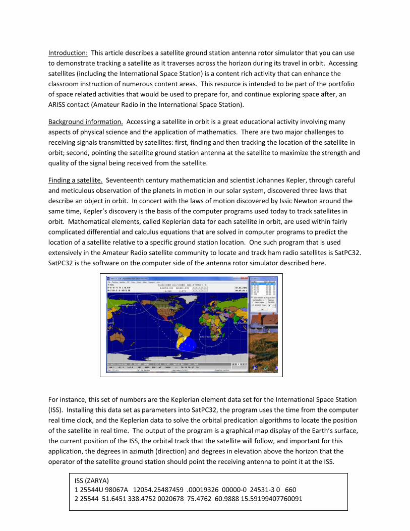
For instance, this set of numbers are the Keplerian element data set for the International Space Station 

(ISS).  Installing this data set as parameters into SatPC32, the program uses the time from the computer 

real time clock, and the Keplerian data to solve the orbital predication algorithms to locate the position 

of the satellite in real time.  The output of the program is a graphical map display of the Earth’s surface, 

the current position of the ISS, the orbital track that the satellite will follow, and important for this 

application, the degrees in azimuth (direction) and degrees in elevation above the horizon that the 

operator of the satellite ground station should point the receiving antenna to point it at the ISS.    

AZ180.0 EL045.0

 

SatPC32 is a multi‐function program in that it not only locates, tracks, and displays the real time position 

of the satellite of interest, but it also outputs commands that can be used to drive the positioning 

system of the ground station antenna (called an AZ/EL rotor, or azimuth/elevation rotor).  It also 

calculates the Doppler frequency shift correction to tune a radio to the proper frequency or channel to 

clearly receive the signal being transmitted by the satellite.  One of the more interesting things about 

using satellites in the classroom, with velocities on the order of 17,000 miles per hour, is that the 

velocity differences are significant when compared to the speed of light, and therefore Doppler shift is 

easy to detect (right between the eyes easy).  The antenna pointing information is very straight forward 

as illustrated by this sample of data from a satellite pass being tracked by SatPC32. 

 

 

Antenna Pointing.  There are a couple of components to the satellite ground station antenna system 

that need to be discussed.  First, let’s take a look at the antenna itself to understand the advantage of 

pointing the antenna at the satellite in the first place.  Then we will take a look at the motor (rotor) 

system that is used to point the antenna. 

Satellites have a limited amount of power to work with.  Generally power for a satellite’s systems are 

provided by solar panels with some rechargeable batteries in parallel with the solar panels to provide 

some backup power when the satellite is not in sunlight (eclipse)…which can happen frequently (but not 

for extended periods of time) depending on the type and orientation of the satellite orbit.  The amount 

of power that can be generated by a solar panel is a function of the angle of incidence of the light rays 

striking the panel surface (direct rays perpendicular to the solar panel surface provide the most 

potential to generate power) and the amount of panel surface area available (more surface area, more 

power can be generated).  Current satellite technology has reduced the size of satellites to cubes with 

10 centimeters on a side, and even smaller satellites, 5 cm sided cubes, are imminent for launch.  These 

small packages may be less expensive to get into space, but the amount of solar panel surface area 

available to generate power is limited…necessitating limited power for system operation, i.e., low power 

transmitters for data links.  Therefore, not only are the radio signals being transmitted attenuated 

significantly because of the long distances traveled between the satellite and the surface of the Earth, 

but also the transmitted signals start out with low power because of the available power budget is 

restricted by the small size of the satellite.  

 A standard technique to boost the apparent signal strength of a received (or transmitted) radio signal is 

to focus or direct the available radio frequency energy in the desired direction by the use of directional 

antennas (one common type of directional or “beam” antenna is called a Yagi, another common type 

that students will be familiar with are the “dish” antennas). The illustration below has a “crossed yagi” 

antenna in the background and a “helix” antenna with a dish reflector in the foreground, both antennas 

designed for satellite reception. 

 

 

 

 

 

 

 

 

The illustration below is of the radiation of radio energy from a typical yagi antenna.  The further the 

trace or plot is away from the center of the polar origin (where the antenna is located), the stronger the 

signal is in that compass direction.  Here the antenna is “pointing” toward 90 degrees or to the right.  

Therefore, you would point the yagi at the transmitter to achieve the best “gain” or signal from that 

transmitter.  Pointing off to one side or the other, or away from the transmitter, would actually 

attenuate or decrease the strength of the received signal. 

 

 

 

 

 

 

 

 

This is another picture of a typical satellite ground station antenna system.  There are actually three yagi 

antennas in this antenna system, one for the VHF band, one for the UHF band (both used for satellite 

communications), and the center yagi is a dedicated VHF band antenna for accessing NOAA weather 

satellites. 

 

 

 

 

 

 

 

 

  

 

 

 

 

Directional antennas use the physics of constructive and destructive wave interference to direct the 

radio energy in a desired direction (through conservation of energy).  Directional antennas, by necessity, 

are larger and more cumbersome than simple non‐directional antennas which makes them not practical 

for small satellites.  Consequently, satellites will use non‐directional antennas, putting the responsibility 

for “boosting” the weak transmissions from the satellite squarely on the ground station designer and 

operator. 

It is generally not practical to manually rotate and point the antenna (though it is very possible, 

particularly with small, hand‐held antennas) and some sort of motor system called a rotor is used.  The 

rotor system is actually two independent motors, one turns the antenna in azimuth (compass direction 

relative to True North), the other turns the antenna in elevation above the horizon.  There is a calibrated 

feedback system built in and attached to the motor shafts so that the controlling computer can sense 

the direction the antenna is pointed, and the computer can either command a change in direction, or it 

can command the motors to stop when the antennas achieve the desired pointing angles. 

In the simplest terms, the rotor control computer will: 

1. Receive the updated antenna pointing position from SatPC32 in degrees azimuth (AZ) and 

elevation (EL). 

2. Read the current AZ and EL position of the antennas. 

3. Determine the direction of travel, clock‐wise, counter clock‐wise; up, down, and close motor 

control relays or switches to cause the motors to turn the antenna in the desired direction. 

4. While the antenna is moving, the controller continuously monitors the progress of the antenna 

movement and compares the instantaneous position to the desired position. 

5. When the antenna is pointed in the desired direction, the controller turns off the motors and 

waits for the next command position from SatPC32. 

When you understand the technology involved, it is fascinating to watch the system at work.  The 

purpose of the antenna rotor simulator is to allow your students to experience an antenna rotor system 

in action within the comfort of the classroom. 

 

Satellite Antenna Rotor Simulator.  Just like the real rotor system, the simulator consists of four basic 

parts: the satellite tracking program SatPC32 that has already been described, an interface that 

translates the position updates from SatPC32 into switch manipulations to move the rotors (motors), 

the rotors, and of course the antenna.  The antenna is also a model to simulate the actual yagi antenna 

so that the system will fit on a table top. 

 

 

 

 

 

 

 

 

 

The main component of the simulator’s controller is a small, dedicated computer called a PIC 

(programmable interface controller).  The PIC has a computer program that simply does the steps 

described in the previous section.  This is the circuit diagram of the controller hardware and the circuit 

board of the interface. 

 

  

 

 

 

 

 

 

 

 

 

The other major components of the simulator are the servo motors that are used to rotate the antenna.  

Servos are another interesting bit of technology.  Servos are basically high ratio geared motors with 

position determining electronics integrated into the servo packages.  There are variety of servos 

available, the ones used in the simulator are standard 180 degree servos that are common in radio 

controlled hobby airplanes, boats, and cars.  Because the technology is used in so many robotic 

applications, it is worth spending a little time understanding what is going on inside those black boxes. 

The power supplied (5 volts DC) to the servo motor is parceled through a controlling feedback loop.  The 

servo motors are commanded to a specific “clock” position by using pulse width modulation (PWM). In 

other words, a stream of pulses are sent to the servo controlling electronics at 20 mS intervals, the 

width of the pulse determines the clock position the servo motor will turn to, and maintain, as long as 

the pulse “train” continues, or a new pulse width is sent to drive the motors to a new clock position.  In 

a 180 degree servo as used in the simulator, by convention, a pulse width of 1 mS will drive the servo 

motor to the 3 o’clock position (clockwise rotation), 1.5 mS pulse width will drive the servo to the 12 

o’clock position, and 2 mS pulse width will drive the servo to the 9 o’clock position (counter clockwise 

rotation).  Intermediate clock positions are determined by intermediate pulse widths between 1 mS and 

2 mS.   This illustration is of an oscilloscope screen shot that shows PWM signals being sent to two 

servos, the blue trace (wide pulse)  drives the attached servo to the 9 o’clock position, the red trace 

(narrow pulse) drives the attached servo to the 3 o’clock position (with 20 mS between pulses).   

 

 

 

 

 

 

 

 

 

 

 

 

 

 

 

Here is a little more detail on what is going on inside of a servo.  Physically, there are a number of gears 

that gear down a high speed, low torque motor and connect the motor shaft at lower speed and higher 

torque to an output shaft that drives outside mechanics.  

 

 

 

 

 

 

 

 

The central part of the servo electronics includes a specialized oscillator integrated circuit called a 555 

timer and a comparator operational amplifier.  The 555 timer is an oscillator that generates a stream of 

 

pulses, the width of the pulses is controlled by an internal variable resistor that is connected by gears to 

the servo motor shaft.  The comparator does what the device name implies, it compares two input 

signals and outputs one state if input A is greater than input B, and outputs the opposite state if input A 

is less than input B. 

Remember, the pulse widths produced by the 555 timer are determined by a variable resistor connected 

to the motor shaft.  The user (you) commands a position change for the servo by sending a stream of 

pulses of a specified width…for this example let’s say 1.5 mS.  These 1.5 mS pulses go to one input of the 

comparator.  The 555 timer is simultaneously sending pulses to the other channel of the comparator, 

the pulse widths determined by the motor shaft position.  If the two input channels are the same (same 

pulse widths) this indicates the servo shaft is at the desired position and power is turned off to the 

motor.  However, if the two input channels are not the same, this situation is detected by the 

comparator and the comparator will feed current to the servo motor of the correct polarity to drive the 

motor in the correct direction.  The output pulses of the 555 timer then are continuously compared to 

the user input pulses in a feedback loop.  When it is detected that the 555 timer pulses are the same 

width, the motor shaft is in the right position, and the current to the motor is turned off.  This schematic 

illustrates this feedback loop process. 

 

 

 

 

 

 

 

 

 

 

A 180 degree servo works fine for the elevation rotor of the simulator, but by itself, will not work for the 

360 degree rotation required for azimuth.  The simple solution in the simulator is to piggy‐back two 180 

degree servos for the azimuth rotor.  The bottom servo turns the whole system the first 180 degrees of 

azimuth rotation, the middle servo then takes over and turns the additional 180 degrees to achieve a full 

360 degrees azimuth rotation.  The software installed in the PIC takes care of keeping that all straight. 

 

 

 

 

 

 

 

 

 

 

 

There is another important teachable moment that can be addressed with the simulator, and that is the 

various number systems used by computers to communicate between the computer microprocessor 

and the input/output device, i.e., printed characters displayed on a computer monitor.  Computers deal 

with binary numbers, which is a number system based on 2 discrete values (on or off, 1 or 0) as opposed 

to the decimal system we are used to working with.  Additionally, since computers can only deal with 

binary numbers, any text characters, like you are reading right now, need to be translated into numbers 

that represent the individual characters so that the computer can deal with them appropriately. 

Significant care and attention must be given to what number system is being used or there may be 

catastrophic results.  The numbering system commonly used by a computer to communicate with the 

outside world (to a monitor, or even between computers) is called ASCII.  The following table is an 

extract of the ASCII data set (this extract contains the character set of the data sent by SatPC32 to 

control the antenna position). 

 

 

 

 

 

 

 

ASCII TABLE EXTRACT 

Character  ASCII Value Decimal  ASCII Value Hexadecimal  ASCII Value Binary 

A  65  0x41  0100 0001 

Z  90  0x5a  0101 1010 

E  69  0x45  0100 0101 

L  76  0x4c  0100 1100 

[] Space  32  0x20  0010 0000 

. Period  46  0x2e  0010 1110 

0  48  0x30  0011 0000 

1  49  0x31  0011 0001 

2  50  0x32  0011 0010 

3  51  0x33  0011 0011 

4  52  0x34  0011 0100 

5  53  0x35  0011 0101 

6  54  0x36  0011 0110 

7  55  0x37  0011 0111 

8  56  0x38  0011 1000 

9  57  0x39  0011 1001 

 

So when the computer wants to display the letter “A”, it will actually send the ASCII number that 

represents the letter A…65 in decimal or 01000001 in binary…to the monitor.  Or, in the case of SatPC32, 

if the program is commanding the antenna to point to the AZ of 180 degrees and EL of 45 degrees 

([AZ180.0 EL045.0]), the computer would actually send the following numbers (in decimal form here): 

65,90,49,56,48,46,32,69,76,48,53,53,46,48 

There is one more complicating factor that must be remembered and dealt with inside the rotor 

controller software, numbers are received as their ASCII representations of the number (the character 1, 

not the number 1).  Before any mathematics or comparisons of numbers can be performed, the ASCII 

representations must be converted into the actual numerical values…a simple matter of subtracting 48 

from the ASCII values does the trick…but important none the less. 

The serial communications between the computer and attached devices is also a teachable moment.  

You have already seen the PWM signal sent by a computer to control a servo, this is a screen shot of the 

serial stream being sent by the computer to send ASCII values to attached devices. 

 

 

 

 

 

 

 

 

 

 

 

 

 

 

 

 

In this oscilloscope digital pattern, when the trace is high, that represents binary 1, when it is low, that 

represents binary 0, and the individual bits are defined by a time interval width (defined as baud).  So 

looking at the trace from left to right, the first change from high to low is called the “start bit”, this 

signals the attached device that data transmission is about to commence.  The first time interval (bit) is 

also low, so a “0” bit is collected.  The rise to high is held for three time intervals, so “1 1 1” bits are 

collected.  The next time interval is low, “0”, the next is high, “1”, and finally low for two more time 

intervals for “0 0”.  The final accumulation of 8‐bits (1‐byte) that is transmitted is “01110100” which is 

116 decimal or the letter “t” in ASCII. 

Simulator setup and operation.  Now on to the fun stuff.  Install SatPC32 using the default settings.  Go 

to the Setup/Observer drop down menu and enter your location latitude and longitude (this is another 

teachable moment…converting between the different degrees/minute/second formats used for lat/long 

depending on the application).  This is the setup for the author’s location in Gales Ferry, Connecticut. 

 

 

 

 

 

 

Determine the comm. port number for your USB to serial converter.  Then go to the Setup/Rotor Setup 

drop down menu.  In the rotor interface/controller drop down select SAEBRTrackBox and then enter the 

comm. port and other parameters as illustrated here. 

 

 

 

 

 

 

 

 

You will need to update the Keplerian data and ensure your computer clock is accurate.  To update the 

Keps, go to the Satellite drop down menu, select the set of satellites you would like to track 

(amateur.txt is a good place to start), and click on the Update Keps button.  SatPC32 will connect you to 

the appropriate server for downloading the most current Kep data.  For the casual satellite user, 

updating the Keps once a week is adequate (the Keps change because of orbital drag…another teachable 

moment).   It will take some time to learn the intricacies of the SatPC32 program, I cannot cover them all 

here.     Numerous help files can be found under the "?" menu. 

To track a particular satellite, click on the letter for the desired satellite in the bottom right corner of the 

display, then click on the “R” in the top left of the display (it changes to R+), and when the satellite is 

within range of your location, the simulator will move the antenna to track the satellite.  You can test 

your system operation by clicking on Rotor in the menu bar, and manually entering different EL and AZ 

degrees into the appropriate boxes, and press Execute.  The rotor simulator will turn to that position. 

Rotor Simulator Construction.  If you would like to construct your own rotor simulator and do not want 

deal with the complexity of PIC programming in C code, a simpler (but more expensive) alternative is to 

use a Parallax BStamp Homework Board.  The homework board has plugs or jacks that accept the plugs 

on servo motors.  The BStamp uses PBasic language which is relatively more intuitive and easy to learn.  

PBasic with the BStamp is an excellent platform for learning microcontroller basics and programming.  

Exceptional instructional materials for the BStamp are available at www.parallax.com.  Sample code and 

a circuit diagram for the rotor simulator using the homework board can be located at link that 

accompanied this document. 

The rotor simulator that you see illustrated here is available through the ARRL Education and 

Technology Grant Program www.arrl.org/etp‐grants.  Interested teachers can obtain a copy for use in 

their classrooms.  For those more adventurous who would like to construct their own duplicate 

simulator, or would like to modify it to experiment on your own, the PIC “C” code software is available 

at this web at link that accompanied this document. 

In either case, you will have to construct your own antenna model for the simulator.  The one illustrated 

in this article is constructed out of a kebab skewer and hot glue.  More rigorous details on antenna 

construction are available through numerous web sources or contained in the ARRL Antenna Handbook. 

SUMMARY.  This article only scratches the surface and is intended to introduce the concept of the 

satellite antenna rotor simulator.  To truly take advantage of the educational opportunities afforded by 

accessing satellites in the classroom, more detailed study is required, but it is a well worth the effort.  

For assistance and more information contact the ARRL ETP at 860‐594‐0296, or 860‐381‐5335, or via e‐

mail to mspencer@arrl.org.  You can also find resources at AMSAT.org.