ARRL HANDBOOK - Antenna Project
114
Antennas & Projects 20. 1 ANTENNA BASICS very ham needs at least one antenna, and most hams have built one. This chapter, by Chuck Hutchinson, K8CH, covers theory and construction of antennas for most radio amateurs. Here you’ll find simple verticals and dipoles, as well as quad and Yagi projects and other antennas that you can build and use. The amount of available space should be high on the list of factors to consider when selecting an antenna. Those who live in urban areas often must accept a compromise antenna for the HF bands because a city lot won’t accommodate full-size wire dipoles, end-fed systems or high supporting struc- tures. Other limitations are imposed by the amount of money available for an antenna system (including supporting hardware), the number of amateur bands to be worked and local zoning ordinances. Operation objectives also come into play. Do you want to dedicate yourself to serious contesting and DXing? Are you looking for general-purpose operation that will yield short- and long-haul QSOs during periods of good propagation? Your answers should result in selecting an antenna that will meet your needs. You might want to erect the biggest and best collection of antennas that space and finances will allow. If a modest system is the order of the day, then use whatever is practical and accept the perfor- mance that follows. Practically any radiator works well under some propagation conditions, assuming the radiator is able to accept power and radiate it at some useful angle. Any antenna is a good one if it meets your needs! In general, the height of the antenna above ground is the most critical factor at the higher end of the HF spectrum, that is from roughly 14 through 30 MHz. This is because the antenna should be clear of conductive objects such as power lines, phone wires, gutters and the like, plus high enough to have a low radiation angle. Lower frequency antennas, operating between 2 and 10 MHz, should also be kept well away from conductive objects and as high above ground as possible if you want good performance. Antenna Polarization Most HF-band antennas are either vertically or horizontally polarized, although circular polarization is possible, just as it is at VHF and UHF. Polarization is determined by the position of the radiating element or wire with respect to the earth. Thus a radiator that is parallel to the earth radiates horizontally, while an antenna at a right angle to the earth (vertical) radiates a vertical wave. If a wire antenna is slanted above earth, it radiates waves that have both a vertical and a horizontal component. 20 Antennas & Projects E
Transcript of ARRL HANDBOOK - Antenna Project

Antennas & Projects 20.1
ANTENNA BASICS
very ham needs at least one antenna, and most hams have built one. This chapter, by ChuckHutchinson, K8CH, covers theory and construction of antennas for most radio amateurs. Hereyou’ll find simple verticals and dipoles, as well as quad and Yagi projects and other antennas that
you can build and use.The amount of available space should be high on the list of factors to consider when selecting an
antenna. Those who live in urban areas often must accept a compromise antenna for the HF bandsbecause a city lot won’t accommodate full-size wire dipoles, end-fed systems or high supporting struc-tures. Other limitations are imposed by the amount of money available for an antenna system (includingsupporting hardware), the number of amateur bands to be worked and local zoning ordinances.
Operation objectives also come into play. Do you want to dedicate yourself to serious contesting andDXing? Are you looking for general-purpose operation that will yield short- and long-haul QSOs duringperiods of good propagation? Your answers should result in selecting an antenna that will meet yourneeds. You might want to erect the biggest and best collection of antennas that space and finances willallow. If a modest system is the order of the day, then use whatever is practical and accept the perfor-mance that follows. Practically any radiator works well under some propagation conditions, assumingthe radiator is able to accept power and radiate it at some useful angle. Any antenna is a good one if itmeets your needs!
In general, the height of the antenna above ground is the most critical factor at the higher end of theHF spectrum, that is from roughly 14 through 30 MHz. This is because the antenna should be clear ofconductive objects such as power lines, phone wires, gutters and the like, plus high enough to have a lowradiation angle. Lower frequency antennas, operating between 2 and 10 MHz, should also be kept wellaway from conductive objects and as high above ground as possible if you want good performance.
Antenna Polarization
Most HF-band antennas are either vertically or horizontally polarized, although circular polarizationis possible, just as it is at VHF and UHF. Polarization is determined by the position of the radiatingelement or wire with respect to the earth. Thus a radiator that is parallel to the earth radiates horizontally,while an antenna at a right angle to the earth (vertical) radiates a vertical wave. If a wire antenna is slantedabove earth, it radiates waves that have both a vertical and a horizontal component.
20Antennas & Projects
E

20.2 Chapter 20
For best results in line-of-sight communications, antennas at both ends of the circuit should have thesame polarization; cross polarization results in many decibels of signal reduction. It is not essential forboth stations to use the same antenna polarity for ionospheric propagation (sky wave). This is becausethe radiated wave is bent and it tumbles considerably during its travel through the ionosphere. At the farend of the communications path the wave may be horizontal, vertical or somewhere in between at anygiven instant. On multihop transmissions, in which the signal is refracted more than once from theionosophere, and subsequently reflected from the Earth’s surface during its travel, considerable polar-ization shift will occur. For that reason, the main consideration for a good DX antenna is a low angleof radiation rather than the polarization.
Antenna Bandwidth
The bandwidth of an antenna refers generally to the range of frequencies over which the antenna canbe used to obtain good performance. The bandwidth is often referenced to some SWR value, such as,“The 2:1 SWR bandwidth is 3.5 to 3.8 MHz.” Popular amateur usage of the term “bandwidth” most oftenrefers to the 2:1 SWR bandwidth. Other specific bandwidth terms are also used, such as the gainbandwidth and the front-to-back ratio bandwidth.
For the most part, the lower the operating frequency of a given antenna design, the narrower is thebandwidth. This follows the rule that the bandwidth of a resonant circuit doubles as the frequency ofoperation is doubled, assuming the Q is the same for each case. Therefore, it is often difficult to coverall of the 160 or 80-m band for a particular level of SWR with a dipole antenna. It is important torecognize that SWR bandwidth does not always relate directly to gain bandwidth. Depending on theamount of feed-line loss, an 80-m dipole with a relatively narrow 2:1 SWR bandwidth can still radiatea good signal at each end of the band, provided that an antenna tuner is used to allow the transmitter toload properly. Broadbanding techniques, such as fanning the far ends of a dipole to simulate a conicaltype of dipole, can help broaden the SWR response curve.
Current and Voltage Distribution
When power is fed to an antenna, the current and voltage vary along its length. The current is nearlyzero (a current node) at the ends. The current does not actually reach zero at the current nodes, becauseof capacitance at the antenna ends. Insulators, loops at the antenna ends, and support wires all contributeto this capacitance, which is also called the “end effect.” In the case of a half-wave antenna there is acurrent maximum (a current loop) at the center.
The opposite is true of the RF voltage. That is, there is a voltage loop at the ends, and in the case ofa half-wave antenna there is a voltage minimum (node) at the center. The voltage is not zero at its nodebecause of the resistance of the antenna, which consists of both the RF resistance of the wire (ohmic lossresistance) and the radiation resistance. The radiation resistance is the equivalent resistance that woulddissipate the power the antenna radiates, with a current flowing in it equal to the antenna current at acurrent loop (maximum). The loss resistance of a half-wave antenna is ordinarily small, compared withthe radiation resistance, and can usually be neglected for practical purposes.
Impedance
The impedance at a given point in the antenna is determined by the ratio of the voltage to the currentat that point. For example, if there were 100 V and 1.4 A of RF current at a specified point in an antennaand if they were in phase, the impedance would be approximately 71 Ω.
Antenna impedance may be either resistive or complex (that is, containing resistance and reactance).This will depend on whether or not the antenna is resonant at the operating frequency. You need to knowthe impedance in order to match the feeder to the feedpoint. Some operators mistakenly believe that amismatch, however small, is a serious matter. This is not true. The importance of a matched line is

Antennas & Projects 20.3
described in detail in the Transmission Lines chapter of this book. The significance of a perfect matchbecomes more pronounced only at VHF and higher, where feed-line losses are a major factor.
Some antennas possess a theoretical input impedance at the feedpoint close to that of certain trans-mission lines. For example, a 0.5-λ (or half-wave) center-fed dipole, placed at a correct height aboveground, will have a feedpoint impedance of approximately 75 Ω. In such a case it is practical to use a75-Ω coaxial or balanced line to feed the antenna. But few amateur half-wave dipoles actually exhibita 75-Ω impedance. This is because at the lower end of the high-frequency spectrum the typical heightabove ground is rarely more than 1/4 λ. The 75-Ω feed-point impedance is most likely to be realized ina practical installation when the horizontal dipole is approximately 1/2, 3/4 or 1 wavelength aboveground. Coax cable having a 50-Ω characteristic impedance is the most common transmission line usedin amateur work.
Fig 20.1 shows the difference between the effects of perfectground and typical earth at low antenna heights. The effect ofheight on the radiation resistance of a horizontal half-wave an-tenna is not drastic so long as the height of the antenna is greaterthan 0.2 λ. Below this height, while decreasing rapidly to zeroover perfectly conducting ground, the resistance decreases lessrapidly with height over actual ground. At lower heights the resis-tance stops decreasing at around 0.15 λ, and thereafter increasesas height decreases further. The reason for the increasing resis-tance is that more and more of the induction field of the antennais absorbed by the earth as the height drops below 1/4 λ.
Conductor Size
The impedance of the antenna also depends on the diameter ofthe conductor in relation to the wavelength, as indicated inFig 20.2. If the diameter of the conductor is increased, the capaci-tance per unit length increases and the inductance per unit lengthdecreases. Since the radiation resistance is affected relativelylittle, the decreased L/C ratio causes the Q of the antenna to de-crease so that the resonance curve becomes less sharp with changein frequency. This effect is greater as the diameter is increased,and is a property of some importance at the very high frequencieswhere the wavelength is small.
Directivity and Gain
All antennas, even the simplest types, exhibit directive effectsin that the intensity of radiation is not the same in all directionsfrom the antenna. This property of radiating more strongly insome directions than in others is called the directivity of the an-tenna.
The gain of an antenna is closely related to its directivity. Be-cause directivity is based solely on the shape of the directive pat-tern, it does not take into account any power losses that may occurin an actual antenna system. Gain takes into account those losses.
Gain is usually expressed in decibels, and is based on a compari-son with a “standard” antenna—usually a dipole or an isotropicradiator. An isotropic radiator is a theoretical antenna that would,
Fig 20.1—Curves showing theradiation resistance of verticaland horizontal half-wavelengthdipoles at various heights aboveground. The broken-line portionof the curve for a horizontaldipole shows the resistance over“average” real earth, the solidline for perfectly conductingground.
Fig 20.2—Effect of antennadiameter on length for half-wavelength resonance, shown asa multiplying factor, K, to beapplied to the free-space, half-wavelength equation.

20.4 Chapter 20
if placed in the center of an imaginary sphere, evenly illuminate that sphere with radiation. The isotropicradiator is an unambiguous standard, and so is frequently used as the comparison for gain measurements.When the standard is the isotropic radiator in free space, gain is expressed in dBi. When the standard isa dipole, also located in free space, gain is expressed in dBd.
The more the directive pattern is compressed—or focused—the greater the power gain of the antenna.This is a result of power being concentrated in some directions at the expense of others. The directivepattern, and therefore the gain, of an antenna at a given frequency is determined by the size and shapeof the antenna, and on its position and orientation relative to the Earth.
Elevation Angle
For HF communication, thevertical (elevation) angle ofmaximum radiation is of consid-erable importance. You will wantto erect your antenna so that itradiates at desirable angles.Tables 20.1, 20.2 and 20.3 showoptimum elevation angles fromlocations in the continental US.These figures are based on statis-tical averages over all portions ofthe solar sunspot cycle.
Since low angles usually aremost effective, this generallymeans that horizontal antennasshould be high—higher is usuallybetter. Experience shows that sat-isfactory results can be attainedon the bands above 14 MHz withantenna heights between 40 and70 ft. Fig 20.3 shows this effectat work in horizontal dipole an-tennas.
Imperfect Ground
Earth conducts, but is far frombeing a perfect conductor. Thisinfluences the radiation patternof the antennas that we use. Theeffect is most pronounced at highvertical angles (the ones thatwe’re least interested in for long-distance communications) forhorizontal antennas. The conse-quences for vertical antennas aregreatest at low angles, and arequite dramatic as can be clearlyseen in Fig 20.4, where the eleva-
Table 20.1Optimum Elevation Angles to Europe
Upper Lower WestBand Northeast Southeast Midwest Midwest Coast10 m 5° 3° 3° 7° 3°12 m 5° 6° 4° 6° 5°15 m 5° 7° 8° 5° 6°17 m 4° 8° 7° 5° 5°20 m 11° 9° 8° 5° 6°30 m 11° 11° 11° 9° 8°40 m 15° 15° 14° 14° 12°75 m 20° 15° 15° 11° 11°
Table 20.2Optimum Elevation Angles to Far East
Upper Lower WestBand Northeast Southeast Midwest Midwest Coast10 m 4° 5° 5° 5° 6°12 m 4° 8° 5° 12° 6°15 m 7° 10° 10° 10° 8°17 m 7° 10° 9° 10° 5°20 m 4° 10° 9° 10° 9°30 m 7° 13° 11° 12° 9°40 m 11° 12° 12° 12° 13°75 m 12° 14° 14° 12° 15°
Table 20.3Optimum Elevation Angles to South America
Upper Lower WestBand Northeast Southeast Midwest Midwest Coast10 m 5° 4° 4° 4° 7°12 m 5° 5° 6° 3° 8°15 m 5° 5° 7° 4° 8°17 m 4° 5° 5° 3° 7°20 m 8° 8° 8° 6° 8°30 m 8° 11° 9° 9° 9°40 m 10° 11° 9° 9° 10°75 m 15° 15° 13° 14° 14°

Antennas & Projects 20.5
tion pattern for a 40-m verticalhalf-wave dipole located overaverage ground is compared toone located over saltwater. At10° elevation, the saltwater an-tenna has about 7 dB more gainthan its landlocked counterpart.
A vertical antenna may workwell at HF for a ham living in thearea between Dallas, Texas andLincoln, Nebraska. This area ispastoral, has low hills, and richsoil. Ground of this type has verygood conductivity. By contrast,a ham living in New Hampshire,where the soil is rocky and a poorconductor, may not be satisfiedwith the performance of a verti-cal HF antenna.
Fig 20.4—Elevation patterns fora vertical dipole over sea watercompared to average ground. Ineach case the center of thedipole is just over 1/4 λλλλλ high.The low-angle response isgreatly degraded over averageground compared to sea water,which is virtually a perfectground.
Fig 20.3—Elevation patterns fortwo 40-m dipoles over averageground (conductivity of 5 mS/mand dielectric constant of 13) at1/4 λλλλλ (33 ft) and 1/2 λλλλλ (66 ft)heights. The higher dipole hasa peak gain of 7.1 dBi at anelevation angle of about 26°,while the lower dipole has moreresponse at high elevationangles.

20.6 Chapter 20
Dipoles and the Half-Wave AntennaA fundamental form of antenna is a wire whose length is half the transmitting wavelength. It is the
unit from which many more complex forms of antennas are constructed and is known as a dipole antenna.The length of a half-wave in free space is
)MHz(f492)ft(Length = (1)
The actual length of a resonant 1/2-λ antenna will not be exactly equal to the half wavelength in space,but depends on the thickness of the conductor in relation to the wavelength. The relationship is shownin Fig 20.2, where K is a factor that must be multiplied by the half wavelength in free space to obtainthe resonant antenna length. An additional shortening effect occurs with wire antennas supported byinsulators at the ends because of the capacitance added to the system by the insulators (end effect). Thefollowing formula is sufficiently accurate for wire antennas for frequencies up to 30 MHz.
( ) ( ) ( )MHzf
468
MHzf
95.0492ftantennawave-halfofLength =×= (2)
Example: A half-wave antenna for 7150 kHz (7.15 MHz) is 468/7.15 = 65.45 ft, or 65 ft 5 inches.Above 30 MHz use the following formulas, particularly for antennas constructed from rod or tubing.
K is taken from Fig 20.2.
( ) ( )MHzf
K492ftantennawave-halfofLength
×= (3)
( ) ( )MHzf
K5904in.length
×= (4)
Example: Find the length of a half-wave antenna at 50.1 MHz, if the antenna is made of 1/2-inch-diametertubing. At 50.1 MHz, a half wavelength in space is
ft 82.91.50
492 =
From equation 1 the ratio of half wavelength to conductor diameter (changing wavelength to inches) is
( )7.235
inch5.0
1282.9 =×
From Fig 20.2, K = 0.965 for this ratio. The length of the antenna, from equation 3 is
ft 48.91.50965.0492 =×
or 9 ft 53/4 inches. The answer is obtained directly in inches by substitution in equation 4
inches 7.1131.50
965.05904 =×
The length of a half-wave antenna is also affected by the proximity of the dipole ends to nearbyconductive and semiconductive objects. In practice, it is often necessary to do some experimental“pruning” of the wire after cutting the antenna to the computed length, lengthening or shortening it inincrements to obtain a low SWR. When the lowest SWR is obtained for the desired part of an amateurband, the antenna is resonant at that frequency. The value of the SWR indicates the quality of the match

Antennas & Projects 20.7
between the antenna and the feed line. If the lowest SWR obtainable is too high for use with solid-staterigs, a Transmatch or line-input matching network may be used, as described in the Transmission Linesand Station Setup chapters.
Radiation Characteristics
The radiation pattern of a dipole antenna in free space is strongestat right angles to the wire (Fig 20.5). This figure-8 pattern appearsin the real world if the dipole is 1/2 λ or greater above earth and is notdegraded by nearby conductive objects. This assumption is basedalso on a symmetrical feed system. In practice, a coaxial feed linemay distort this pattern slightly, as shown in Fig 20.5. Minimumhorizontal radiation occurs off the ends of the dipole if the antennais parallel to the earth.
As an antenna is brought closer to ground, the elevation patternpeaks at a higher elevation angle as shown in Fig 20.3. Fig 20.6illustrates what happens to the directional pattern as antenna heightchanges. Fig 20.6C shows that there is significant radiation off theends of a low horizontal dipole. For the 1/2-λ height (solid line), theradiation off the ends is only 7.6 dB lower than that in the broadsidedirection.
Feed Methods
Most amateurs use either coax or open-wire transmission line.Coax is the common choice because it is readily available, its char-acteristic impedance is close to that of the antenna and it may beeasily routed through or alongwalls and among other cables.The disadvantages of coax are in-creased RF loss and low workingvoltage (compared to that ofopen-wire line). Both disadvan-tages make coax a poor choice forhigh-SWR systems.
Take care when choosing coax.Use 1/4-inch foam-dielectriccables only for low power (25 Wor less) HF transmissions. Solid-dielectric 1/4-inch cables are okayfor 300 W if the SWR is low. Forhigh-power installations, use1/2-inch or larger cables.
The most common two-wiretransmission lines are ladder lineand twin lead. Since the conduc-tors are not shielded, two-wirelines are affected by their envi-ronment. Use standoffs and insu-lators to keep the line several
Fig 20.5—Response of a dipoleantenna in free space, wherethe conductor is along 90° to270° axis, solid line. If thecurrents in the halves of thedipole are not in phase, slightdistortion of the pattern willoccur, broken line. This illus-trates case where balun is notused on a balanced antenna fedwith unbalanced line.
Fig 20.6—At A, elevation re-sponse pattern of a dipoleantenna placed 1/2 λλλλλ above aperfectly conducting ground. AtB, the pattern for the sameantenna when raised to onewavelength. For both A and B,the conductor is coming out ofthe paper at right angle. Cshows the azimuth patterns ofthe dipole for the two heights atthe most-favored elevationangle, the solid-line plot for the1/2-λλλλλ height at an elevation angleof 30°, and the broken-line plotfor the 1-λλλλλ height at an elevationangle of 15°. The conductor in Clies along 90° to 270° axis.

20.8 Chapter 20
inches from structures or other conductors. Ladder line has very low loss (twin lead has a little more),and it can stand very high voltages (SWR) as long as the insulators are clean.
Two-wire lines are usually used in balanced systems, so they should have a balun at the transition toan unbalanced transmitter or coax. A Transmatch will be needed to match the line input impedance tothe transmitter.
Baluns
A balun is a device for feeding a balanced load with an unbalanced line, or vice versa (see theTransmission Lines chapter of this book). Because dipoles are balanced (electrically symmetrical abouttheir feed-points), a balun should be used at the feed-point when a dipole is fed with coax. When coaxfeeds a dipole directly (as in Fig 20.7), current flows on the outsideof the cable shield. The shield can conduct RF onto the transmitterchassis and induce RF onto metal objects near the system. Shieldcurrents can impair the function of instruments connected to the line(such as SWR meters and SWR-protection circuits in the transmit-ter). The shield current also produces some feed-line radiation,which changes the antenna radiation pattern, and allows objectsnear the cable to affect the antenna-system performance.
The consequences may be negligible: A slight skewing of the an-tenna pattern usually goes unnoticed. Or, they may be significant: FalseSWR readings may cause the transmitter to shut down or destroy theoutput transistors; radiating coax near a TV feed line may cause stronglocal interference. Therefore, it is better to eliminate feed-line radia-tion whenever possible, and a balun should be used at any transitionbetween balanced and unbalanced systems. (The Transmission Lineschapter thoroughly describes baluns and their construction.) Even so,balanced or unbalanced systems without a balun often operate with noapparent problems. For temporary or emergency stations, do not let thelack of a balun deter you from operating.
Practical Dipole Antennas
A classic dipole antenna is 1/2-λ long and fed at the center. Thefeed-point impedance is low at the resonant frequency, f0, and oddharmonics thereof. The impedance is high near even harmonics.When fed with coax, a classic dipole provides a reasonably lowSWR at f0 and its odd harmonics.
When fed with ladder line (see Fig 20.8A) and a Transmatch, theclassic dipole should be usable near f0 and all harmonic frequencies.(With a wide-range Transmatch, it may work on all frequencies.) Ifthere are problems (such as extremely high SWR or evidence of RFon objects at the operating position), change the feed-line length byadding or subtracting 1/8 λ at the problem frequency. A few suchadjustments should yield a workable solution. Such a system is some-times called a “center-fed Zepp.” A true “Zepp” antenna is an end-feddipole that is matched by 1/4 λ of open-wire feed line (see Fig 20.8B).The antenna was originally used on zeppelins, with the dipole trailingfrom the feeder, which hung from the airship cabin. It is intended foruse on a single band, but should be usable near odd harmonics of f0.
Fig 20.7—Method of affixingfeed line to the center of adipole antenna. A plastic blockis used as a center insulator.The coax is held in place by aclamp. A balun is often used tofeed dipoles or other balancedantennas to ensure that theradiation pattern is not dis-torted. See text for explanation.
Fig 20.8—Center-fed multiband“Zepp” antenna (A) and an end-fed Zepp at (B).

Antennas & Projects 20.9
Most dipoles require a little pruning to reach the desired resonant frequency. Here’s a technique tospeed the adjustment.
How much to prune: When assembling the antenna, cut the wire 2 to 3% longer than the calculatedlength and record the length. When the antenna is complete, raise it to the working height and check theSWR at several frequencies. Multiply the frequency of the SWR minimum by the antenna length anddivide the result by the desired f0. The result is the finished length; trim both ends equally to reach thatlength and you’re done.
Loose ends: Here’s another trick, if you use nonconductive end support lines. When assembling theantenna, mount the end insulators in about 5% from the ends. Raise the antenna and let the ends hangfree. Figure how much to prune and cut it from the hanging ends. If the pruned ends are very long, wrapthem around the insulated line for support.
Dipole Orientation
Dipole antennas need not be installed in a horizontal straight line. They are generally tolerant ofbending, sloping or drooping as required by the antenna site. Remember, however, that dipole antennasare RF conductors. For safety’s sake, mount all antennas away from conductors (especially power lines),combustibles and well beyond the reach of passersby.
A sloping dipole is shown in Fig 20.9. This antenna is often usedto favor one direction (the “forward direction” in the figure). Witha nonconducting support and poor earth, signals off the back areweaker than those off the front. With a nonconducting mast and goodearth, the response is omnidirec-tional. There is no gain in anydirection with a nonconductingmast.
A conductive support such as atower acts as a parasitic element.(So does the coax shield, unless itis routed at 90° from the antenna.)The parasitic effects vary withearth quality, support height andother conductors on the support(such as a beam at the top). Withsuch variables, performance isvery difficult to predict.
Losses increase as the antennaends approach the support or theground. To prevent feed-line ra-diation, route the coax away fromthe feed-point at 90° from the an-tenna, and continue on that lineas far as possible.
An Inverted V antenna appearsin Fig 20.10. While “V” accu-rately describes the shape of thisantenna, this antenna should notbe confused with long-wire Vantennas, which are highly direc-
Fig 20.9—Example of a sloping1/2-λλλλλ dipole, or “full sloper.” Onthe lower HF bands, maximumradiation over poor to averageearth is off the sides and in the“forward direction” as indi-cated, if a nonconductivesupport is used. A metal sup-port will alter this pattern byacting as a parasitic element.How it alters the pattern is acomplex issue depending onthe electrical height of the mast,what other antennas are locatedon the mast, and on the con-figuration of guy wires.
Fig 20.10—At A, details for aninverted V fed with open-wireline for multiband HF operation.A Transmatch is shown at B,suitable for matching the an-tenna to the transmitter over awide frequency range. Theincluded angle between the twolegs should be greater than 90°for best performance.

20.10 Chapter 20
tive. The radiation pattern and dipole impedance depend on the apexangle, and it is very important that the ends do not come too close tolossy ground.
Bent dipoles may be used where antenna space is at a premium.Fig 20.11 shows several possibilities; there are many more. Bendingdistorts the radiation pattern somewhat and may affect the imped-ance as well, but compromises are acceptable when the situationdemands them. When an antenna bends back on itself (as inFig 20.11B) some of the signal is canceled; avoid this if possible.
Remember that current produces the radiated signal, and currentis maximum at the dipole center. Therefore, performance is bestwhen the central area of the antenna is straight, high and clear ofnearby objects. Be safe! Keep any bends, sags or hanging ends wellclear of conductors (especially power lines) and combustibles, andbeyond the reach of persons.
Multiband Dipoles
There are several ways to construct coax-fed multiband dipolesystems. These techniques apply to dipoles of all orientations. Eachmethod requires a little more work than a single dipole, but the ma-terials don’t cost much.
Parallel dipoles are a simple and convenient answer. See Fig 20.12.Center-fed dipoles present low-impedances near f0, or its odd har-monics, and high impedances elsewhere. This lets us construct simplemultiband systems that automatically select the appropriate antenna.Consider a 50-Ω resistor connected in parallel with a 5-kΩ resistor.A generator connected across the two resistors will see 49.5 Ω, and99% of the current will flow through the 50-Ω resistor. When reso-nant and nonresonant antennasare parallel connected, thenonresonant antenna takes littlepower and has little effect on thetotal feed-point impedance.Thus, we can connect severalantennas together at the feed-point, and power naturally flowsto the resonant antenna.
There are some limits, how-ever. Wires in close proximitytend to couple and produce mu-tual inductance. In parallel di-poles, this means that the reso-nant length of the shorter dipoleslengthens a few percent. Shorterantennas don’t affect longer onesmuch, so adjust for resonance inorder from longest to shortest.Mutual inductance also reduces
Fig 20.11—When limited spaceis available for a dipole an-tenna, the ends can be bentdownward as shown at A, orback on the radiator as shownat B. The inverted V at C can beerected with the ends bentparallel with the ground whenthe available supporting struc-ture is not high enough.
Fig 20.12—Multiband antenna using paralleled dipoles, all con-nected to a common 50 or 75-ΩΩΩΩΩ coax line. The half-wavedimensions may be either for the centers of the various bands orselected for favorite frequencies in each band. The length of a halfwave in feet is 468/frequency in MHz, but because of interactionamong the various elements, some pruning for resonance may beneeded on each band. See text.
Antennas & Projects 20.11
the bandwidth of shorter dipoles, so a Transmatch may be needed to achieve an acceptable SWR acrossall bands covered. These effects can be reduced by spreading the ends of the dipoles.
Also, the power-distribution mechanism requires that only one of the parallel dipoles is near resonanceon any amateur band. Separate dipoles for 80 and 30 m should not be parallel connected because thehigher band is near an odd harmonic of the lower band (80/3 ≈ 30) and center-fed dipoles have lowimpedance near odd harmonics. (The 40 and 15-m bands have a similar relationship.) This means thatyou must either accept the lower performance of the low-band antenna operating on a harmonic or erecta separate antenna for those odd-harmonic bands. For example, four parallel-connected dipoles cut for80, 40, 20 and 10 m (fed by a single Transmatch and coaxial cable) work reasonably on all HF bandsfrom 80 through 10 m.
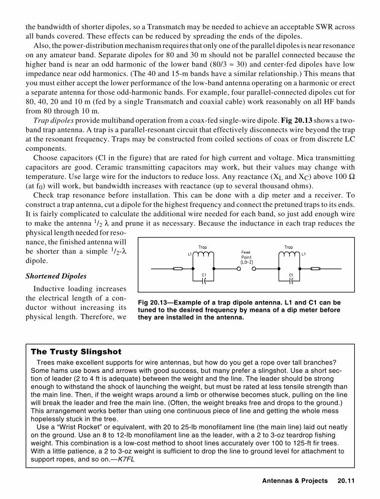
Trap dipoles provide multiband operation from a coax-fed single-wire dipole. Fig 20.13 shows a two-band trap antenna. A trap is a parallel-resonant circuit that effectively disconnects wire beyond the trapat the resonant frequency. Traps may be constructed from coiled sections of coax or from discrete LCcomponents.
Choose capacitors (Cl in the figure) that are rated for high current and voltage. Mica transmittingcapacitors are good. Ceramic transmitting capacitors may work, but their values may change withtemperature. Use large wire for the inductors to reduce loss. Any reactance (XL and XC) above 100 Ω(at f0) will work, but bandwidth increases with reactance (up to several thousand ohms).
Check trap resonance before installation. This can be done with a dip meter and a receiver. Toconstruct a trap antenna, cut a dipole for the highest frequency and connect the pretuned traps to its ends.It is fairly complicated to calculate the additional wire needed for each band, so just add enough wireto make the antenna 1/2 λ and prune it as necessary. Because the inductance in each trap reduces thephysical length needed for reso-nance, the finished antenna willbe shorter than a simple 1/2-λdipole.
Shortened Dipoles
Inductive loading increasesthe electrical length of a con-ductor without increasing itsphysical length. Therefore, we
Fig 20.13—Example of a trap dipole antenna. L1 and C1 can betuned to the desired frequency by means of a dip meter beforethey are installed in the antenna.
Trees make excellent supports for wire antennas, but how do you get a rope over tall branches?Some hams use bows and arrows with good success, but many prefer a slingshot. Use a short sec-tion of leader (2 to 4 ft is adequate) between the weight and the line. The leader should be strongenough to withstand the shock of launching the weight, but must be rated at less tensile strength thanthe main line. Then, if the weight wraps around a limb or otherwise becomes stuck, pulling on the linewill break the leader and free the main line. (Often, the weight breaks free and drops to the ground.)This arrangement works better than using one continuous piece of line and getting the whole messhopelessly stuck in the tree.
Use a “Wrist Rocket” or equivalent, with 20 to 25-lb monofilament line (the main line) laid out neatlyon the ground. Use an 8 to 12-lb monofilament line as the leader, with a 2 to 3-oz teardrop fishingweight. This combination is a low-cost method to shoot lines accurately over 100 to 125-ft fir trees.With a little patience, a 2 to 3-oz weight is sufficient to drop the line to ground level for attachment tosupport ropes, and so on.—K7FL

20.12 Chapter 20
can build physically short dipole antennas by placing inductors in the antenna. These are called “loadedantennas,” and The ARRL Antenna Book shows how to design them. There are some trade-offs involved:Inductively loaded antennas are less efficient and have narrower bandwidths than full-size antennas.Generally they should not be shortened more than 50%.
Building Dipole Antennas
The purpose of this section is to offer information on the actual physical construction of wire antennas.Because the dipole, in one of its configurations, is probably the most common amateur wire antenna, itis used in the following examples. The techniques described here, however, enhance the reliability andsafety of all wire antennas.
Wire
Choosing the right type of wire for the project at hand is the key to a successful antenna—the kind thatworks well and stays up through a winter ice storm or a gusty spring wind storm. What gauge of wireto use is the first question to settle, and the answer depends on strength, ease of handling, cost, avail-ability and visibility. Generally, antennas that are expected to support their own weight, plus the weightof the feed line should be made from #12 wire. Horizontal dipoles, Zepps, some long wires and the likefall into this category. Antennas supported in the center, such as inverted-V dipoles and delta loops, maybe made from lighter material, such as #14 wire—the minimum size called for in the National ElectricalCode.
The type of wire to be used is the next important decision. The wire specifications table in theComponent Data chapter shows popular wire styles and sizes. The strongest wire suitable for antennaservice is copperclad steel, also known as copperweld. The copper coating is necessary for RF servicebecause steel is a relatively poor conductor. Practically all of the RF current is confined to the coppercoating because of skin effect. Copper-clad steel is outstanding for permanent installations, but it canbe difficult to work with. Kinking, which severely weakens the wire, is a constant threat when handlingany solid conductor. Solid-copper wire, either hard drawn or soft drawn, is another popular material.Easier to handle than copper-clad steel, solid copper is available in a wide range of sizes. It is generallymore expensive however, because it is all copper. Soft drawn tends to stretch under tension, so periodicpruning of the antenna may be necessary in some cases. Enamel-coated magnet-wire is a good choicefor experimental antennas because it is easy to manage, and the coating protects the wire from theweather. Although it stretches under tension, the wire may be prestretched before final installation andadjustment. A local electric motor rebuilder might be a good source for magnet wire.
Hook-up wire, speaker wire or even ac lamp cord are suitable for temporary installations. Almost anycopper wire may be used, as long as it is strong enough for the demands of the installation. Steel wireis a poor conductor at RF; avoid it.
It matters not (in the HF region at least) whether the wire chosen is insulated or bare. If insulated wireis used, a 3 to 5% shortening beyond the standard 468/f length will be required to obtain resonance atthe desired frequency, because of the increased distributed capacitance resulting from the dielectricconstant of the plastic insulating material. The actual length for resonance must be determined experi-mentally by pruning and measuring because the dielectric constant of the insulating material varies fromwire to wire. Wires that might come into contact with humans or animals should be insulated to reducethe chance of shock or burns.
Insulators
Wire antennas must be insulated at the ends. Commercially available insulators are made from ce-ramic, glass or plastic. Insulators are available from many Amateur Radio dealers. Radio Shack and localhardware stores are other possible sources.

Antennas & Projects 20.13
Acceptable homemade insulators may be fashioned from a variety of material including (but notlimited to) acrylic sheet or rod, PVC tubing, wood, fiberglass rod or even stiff plastic from a discardedcontainer. Fig 20.14 shows some homemade insulators. Ceramic or glass insulators will usually outlastthe wire, so they are highly recommended for a safe, reliable, permanent installation. Other materialsmay tear under stress or break down in the presence of sunlight. Many types of plastic do not weatherwell.
Many wire antennas require an insulator at the feedpoint. Although there are many ways to connectthe feed line, there are a few things to keep in mind. If you feed your antenna with coaxial cable, youhave two choices. You can install an SO-239 connector on the center insulator and use a PL-259 on theend of your coax, or you can separate the center conductor from the braid and connect the feed linedirectly to the antenna wire. Although it costs less to connect direct, the use of connectors offers severaladvantages.
Coaxial cable braid soaks up water like a sponge. If you do not adequately seal the antenna end of thefeed line, water will find its way into the braid. Water in the feed line will lead to contamination,rendering the coax useless long before its normal lifetime is up. It is not uncommon for water to drip fromthe end of the coax inside the shack after a year or so of service if the antenna connection is not properlywaterproofed. Use of a PL-259/SO-239 combination (or connector of your choice) makes the task ofwaterproofing connections much easier. Another advantage to using the PL-259/SO-239 combinationis that feed line replacement is much easier, should that become necessary.
Whether you use coaxial cable, ladder line, or twin lead to feed your antenna, an often-overlookedconsideration is the mechanical strength of the connection. Wire antennas and feed lines tend to movea lot in the breeze, and unless the feed line is attached securely, the connection will weaken with time.The resulting failure can range from a frustrating intermittent electrical connection to a complete sepa-ration of feed line and antenna. Fig 20.15 illustrates several different ways of attaching the feed line tothe antenna. An idea for supporting ladder line is shown in Fig 20.16.
Putting It Together
Fig 20.17 shows details of antenna construction. Although a dipole is used for the examples, thetechniques illustrated here apply to any type of wire antenna. Table 20.5 shows dipole lengths for theamateur HF bands.
How well you put the pieces together is second only to the ultimate strength of the materials used in
Fig 20.14—Some ideas forhomemade antenna insulators.
Fig 20.15—Some homemade dipole center insulators. The one inthe center includes a built-in SO-239 connector. Others are de-signed for direct connection to the feed line. (See theTransmission Lines chapter for details on baluns.)

20.14 Chapter 20
Fig 20.16—A piece of cut Plexiglas can be used as a center insulator and to support a ladder-linefeeder. The Plexiglas acts to reduce the flexing of the wires where they connect to the antenna.
Fig 20.17—Details of dipole antenna construction. The end insulator connection is shown at A, whileB illustrates the completed antenna. This is a balanced antenna and is often fed with a balun.
Antenna Wire
Antenna Wire(Loop through holes)
Plexiglas
450-ohm Ladder Line
To Antenna Tuner
Secure to Plexiglas withElectrical Tape

Antennas & Projects 20.15
determining how well your antenna will work over the long term.Even the smallest details, such as how you connect the wire to theinsulators (Fig 20.17A), contribute significantly to antenna lon-gevity. By using plenty of wire at the insulator and wrapping ittightly, you will decrease the possibility of the wire pulling loosein the wind. There is no need to solder the wire once it is wrapped.There is no electrical connection here, only mechanical. The highheat needed for soldering can anneal the wire, significantly weak-ening it at the solder point.
Similarly, the feed-line connection at the center insulator shouldbe made to the antenna wires after they have been secured to theinsulator (Fig 20.17B). This way, you will be assured of a goodelectrical connection between the antenna and feed line withoutcompromising the mechanical strength. Do a good job of solder-
ing the antenna and feed-line connections. Use a heavy iron or a torch, and be sure to clean the materialsthoroughly before starting the job. Proper planning should allow you to solder indoors at a workbench,where the best possible joints may be made. Poorly soldered or unsoldered connections will becomeheadaches as the wire oxidizes and the electrical integrity degrades with time. Besides degrading yourantenna performance, poorly made joints can even be a cause of TVI because of rectification. Spray paintthe connections with acrylic for waterproofing.
If made from the right materials, the dipole should give a builder years of maintenance-free service—unless of course a tree falls on it. As you build your antenna, keep in mind that if you get it right the firsttime, you won’t have to do it again for a long time.
Table 20.5Dipole Dimensions forAmateur Bands
Freq Overall LegMHz Length Length28.4 16' 6" 8' 3"24.9 18' 91/2" 9' 43/4"21.1 22' 2" 11' 1"18.1 25' 10" 12' 11"14.1 33' 2" 16' 7"10.1 46' 4" 23' 2"7.1 65' 10" 32' 11"3.6 130' 0" 65' 0"

20.16 Chapter 20
!
An 80-m dipole fed with ladder line is a versatile antenna. If you add a wide-range matchingnetwork, you have a low-cost antenna system that works well across the entire HF spectrum. Countlesshams have used one of these in single-antenna stations and for FieldDay operations.
For best results place the antenna as high as you can, and keepthe antenna and ladder line clear of metal and other conductiveobjects. Despite significant SWR on some bands, system lossesare low. (See the TransmissionLines chapter.) You can makethe dipole horizontal, or youcan install in as an inverted V.ARRL staff analyzed a 135-ftdipole at 50 ft above typicalground and compared that to aninverted V with the center at50 ft, and the ends at 10 ft. Theresults show that on the 80-mband, it won’t make much dif-ference which configurationyou choose. (See Fig 20.18.)The inverted V exhibits addi-tional losses because of itsproximity to ground.
Fig 20.19 shows a comparisonbetween a 20-m flat-top dipoleand the 135-ft flat-top dipolewhen both are placed at 50 ftabove ground. At a 10° elevationangle, the 135-ft dipole has a gainadvantage. This advantage comesat the cost of two deep, but nar-row, nulls that are broadside tothe wire.
Fig 20.20 compares the 135-ftdipole to the inverted-V configu-ration of the same antenna on14.1 MHz. Notice that the in-verted-V pattern is essentiallyomnidirectional. That comes atthe cost of gain, which is less thanthat for a horizontal flat-top di-pole.
As expected, patterns becomemore complicated at 28.4 MHz.As you can see in Fig 20.21, theinverted V has the advantage of a
Fig 20.18—Patterns on 80 m for135-ft, center-fed dipole erectedas a horizontal dipole at 50 ft,and as an inverted V with thecenter at 50 ft and the ends at10 ft. The azimuth pattern isshown at A, where conductorlies in the 90° to 270° plane. Theelevation pattern is shown at B,where conductor comes out ofpaper at right angle. At thefundamental frequency thepatterns are not markedlydifferent.
Fig 20.19—Patterns on 20 mcomparing a standard 1/2-λλλλλdipole and a multiband 135-ftdipole. Both are mountedhorizontally at 50 ft. The azi-muth pattern is shown at A,where conductors lie in the 90°to 270° plane. The elevationpattern is shown at B. Thelonger antenna has four azi-muthal lobes, centered at 35°,145°, 215°, and 325°. Each isabout 2 dB stronger than themain lobes of the 1/2-λλλλλ dipole.The elevation pattern of the135-ft dipole is for one of thefour maximum-gain azimuthlobes, while the elevationpattern for the 1/2-λλλλλ dipole is forthe 0° azimuthal point.

Antennas & Projects 20.17
pattern with slight nulls, but withreduced gain compared to theflat-top configuration.
Installed horizontally, or as aninverted V, the 135-ft center-feddipole is a simple antenna thatworks well from 3.5 to 30 MHz.Bandswitching is handled by aTransmatch that is located nearyour operating position.
Fig 20.20—Patterns on 20 m fortwo 135-ft dipoles. One ismounted horizontally as a flat-top and the other as an invertedV with 120° included anglebetween the two legs. Theazimuth pattern is shown at A,and the elevation pattern isshown at B. The inverted V hasabout 6 dB less gain at the peakazimuths, but has a moreuniform, almost omnidirec-tional, azimuthal pattern. In theelevation plane, the inverted Vhas a fat lobe overhead, makingit a somewhat better antennafor local communication, butnot quite so good for DX con-tacts at low elevation angles.
Fig 20.21—Patterns on 10 m for135-ft dipole mounted horizon-tally and as an inverted V, as inFig 20.20. The azimuth patternis shown at A, and the elevationpattern is shown at B. Onceagain, the inverted-V configura-tion yields a more omni-directional pattern, but at theexpense of almost 8 dB lessgain than the flat-top configura-tion at its strongest lobes.

20.18 Chapter 20
"# $%&
Modern computer programs have made it a lot easier for a ham to evaluate antenna performance.The elevation plots for the 135-ft long center-fed dipole were generated using a sophisticated com-puter program known as NEC, short for “Numerical Electromagnetics Code.” NEC is a general-purpose antenna modeling program, capable of modeling almost any antenna type, from the simplestdipole to extremely complex antenna designs. Various mainframe versions of NEC have been undercontinuous development by US government researchers for several decades.
But because it is a general-purpose program, NEC can be very slow when modeling some anten-nas—such as long-boom, multi-element Yagis. There are other, specialized programs that work onYagis much faster than NEC. Indeed, NEC has developed a reputation for being accurate (if properlyapplied!), but decidedly difficult to learn and use. A number of commercial software developers haverisen to the challenge and created more “user-friendly” versions. Check the ads in QST.
NEC uses a “Method of Moments” algorithm. The mathematics behind this algorithm are prettyformidable to most hams, but the basic principle is simple. An antenna is broken down into a set ofstraight-line wire “segments.” The fields resulting from the current in each segment and from themutual interaction between segments are vector-summed in the far field to create azimuth and eleva-tion-plane patterns.
The most difficult part of using a NEC-type of modeling program is setting up the antenna’s geom-etry—you must condition yourself to think in three-dimensional coordinates. Each end point of a wireis represented by three numbers: an x, y and z coordinate. An example should help sort things out.See Fig A, showing a “model” for a 135-footcenter-fed dipole, made of #14 wire placed 50 ftabove flat ground. This antenna is modeled as asingle, straight wire.
For convenience, ground is located at theorigin of the coordinate system, at (0, 0, 0) feet,directly under the center of the dipole. Thedipole runs parallel to, and above, the y-axis.Above the origin, at a height of 50 feet, is thedipole’s feedpoint. The “wingspread” of thedipole goes toward the left (that is, in the “nega-tive y” direction) one-half the overall length, or–67.5 ft. Toward the right, it goes +67.5 ft. The“x” dimension of our dipole is zero. The dipole’sends are thus represented by two points, whosecoordinates are: (0, –67.5, 50) and (0, 67.5, 50)ft. The thickness of the antenna is the diameterof the wire, #14 gauge.
To run the program you must specify thenumber of segments into which the dipole is divided for the method-of-moments analysis. The guide-line for setting the number of segments is to use at least 10 segments per half-wavelength. In Fig A,our dipole has been divided into 11 segments for 80-m operation. The use of 11 segments, an oddrather than an even number such as 10, places the dipole’s feedpoint (the “source” in NEC-parlance)right at the antenna’s center and at the center of segment number six.
Since we intend to use our 135-foot long dipole on all HF amateur bands, the number of segmentsused actually should vary with frequency. The penalty for using more segments in a program likeNEC is that the program slows down roughly as the square of the segments—double the number andthe speed drops to a fourth. However, using too few segments will introduce inaccuracies, particularlyin computing the feed-point impedance. The commercial versions of NEC handle such nitty-grittydetails automatically.
Let’s get a little more complicated and specify the 135-ft dipole, configured as an inverted-V. Here,as shown in Fig B, you must specify two wires. The two wires join at the top, (0, 0, 50) ft. Now thespecification of the source becomes more complicated. The easiest way is to specify two sources,one on each end segment at the junction of the two wires. If you are using the “native” version of
Fig A

Antennas & Projects 20.19
NEC, you may have to go back to your high-school trigonometry book to figure out how tospecify the end points of our “droopy” dipole,with its 120° included angle. Fig B shows thedetails, along with the trig equations needed.
So, you see that antenna modeling isn’tentirely a cut-and-dried procedure. The com-mercial programs do their best to hide some ofthe more unwieldy parts of NEC, but there’s stillsome art mixed in with the science. And asalways, there are trade-offs to be made—segments versus speed, for example.
However, once you do figure out exactly howto use them, computer models are wonderfultools. They can help you while away a drearywinter’s day, designing antennas on-screen—without having to risk life and limb climbing an
ice-covered tower. And in a relatively short time a computer model can run hundreds, or even thou-sands, of simulations as you seek to optimize an antenna for a particular parameter. Doesn’t thatsound better than trying to optimally tweak an antenna by means of a thousand cut-and-try measure-ments, all the while hanging precariously from your tower by a climbing belt?!—R. Dean Straw,N6BV, Senior Assistant Technical Editor
Fig B

20.20 Chapter 20
%&"## '"###$ "
By Richard Ellers, K8JLK, 426 Central Pkwy, SE, Warren, OH 44483-6213I’ve devised a BASIC program1 you can use to design shortened doublet (dipole) antennas, using
loading coils of known inductance. The program uses common BASIC commands and should run as-is on any IBM PC-compatible or Apple II personal computer. This program is an offshoot and adapta-tion of previously published charts, a formula and a BASIC program. The charts and formula, pub-lished in QST,2 and the original BASIC program, published in CQ,3 were devised to calculate theinductances required to resonate a short doublet, given the overall antenna length, the coil spacingand the element diameter.
The development of my program began when I decided to build a 2-element phased array of shortdoublets, using four surplus mobile coils I’d bought at a hamfest. Checking through my ham maga-zines, I found Dick (K5QY) Sander’s ingenious BASIC version of Jerry Hall’s (then K1PLP, nowK1TD) comprehensive work on the design of off-center-loaded antennas. However, I was in theopposite position: I had the inductance values in hand and needed instead to figure where to place thecoils in an antenna of a certain size.
Not being very adept at higher math, I didn’t even attempt to rewrite Jerry’s formula or K5QY’sprogram. Instead, I revised K5QY’s program by adding a computer routine known as a binary search.Although more often used to seek data in large files, my program uses a binary search as a form ofcomputerized empirical determination (more commonly known as cut-and-try). The search is accu-rate— and rapid. In just seconds, the routine finds the coil spacing that matches the desired antennato the existing inductance.
I wrote the program to find the coil spacing for a single antenna (and for a series of 10 antennas)between two specified lengths. Incidentally, because the program actually calculates the center-to-coil distance (as did K5QY’s version), it can be used to design short vertical antennas, but you mustenter twice the desired overall length. As with K5QY’s program, mine handles antenna elements ofwire or tubing, the diameters being entered in decimal fractions of an inch where necessary. To keepthe program short and simple, I omitted K5QY’s optional wire table. (You can find such a wire table inChapter 24, Component Data, or use the following as a guide: 22-gauge wire has a diameter of0.025 inch; 10-gauge wire’s diameter is 0.101 inch.)
Program error traps catch (and explain) parameter combinations that don’t match the given induc-tor. One trap catches dimensions that would normally put the program in an endless loop. I’ve testedmy program for many configurations and frequencies using inductances first determined by K5QY’sprogram: The results matched every time.
Notes1 The software contains ASCII QBASIC files for both IBM-compatible and Mac computers in file
ELLERS.EXE. It is available at the ARRL Web site. See page vii.2 J. Hall, “Off-Center-Loaded Antennas,” QST, Sep 1974, pp 28-34 and 58.3 D. Sander, “A Computer Designed Loaded Dipole Antenna,” CQ, Dec 1981, p 44.

Antennas & Projects 20.21
!!()*+),)-
This antenna was designed for amateurs with limited space who also wanted to operate the low bands.It was first described in July 1992 QST by A. C. Buxton, W8NX, and features innovative coaxial-cabletraps.
Fig 20.25 shows the antenna layout; it is resonant at 1.865, 3.825, and 7.225 MHz. The antenna ismade of #14 stranded wire and two pairs of coaxial traps. Construction is conventional in most respects,except for the high inductance-to-capacitance (L/C) ratio that results from the unique trap construction.
The traps use two series-connected coil layers, wound in the same direction using RG-58 coaxialcable’s center conductor, together with the insulation over the center conductor. The black outerjacket from the cable is stripped and discarded. The shield braid is also removed from the cable(pushing is easier than pulling the shield off). No doubt you will want to save the braid for use in otherprojects. RG-58 with a stranded center conductor is best for this project. Fig 20.26 shows the traps.The 3.8-MHz trap is shown with the weatherproofing cover of electrical tape removed to showconstruction details.
Precautions and Trap Specifications
With this trap-winding configuration, there are two thicknesses of coax dielectric material between
Fig 20.25—The W8NX trap dipole resonates in the SSB portions of the 40, 80 and 160-m bands. Theantenna is 124 ft long.
(B)
Fig 20.26—The W8NX coaxial-cable traps use two layeredwindings in series to provide anunusually high inductance-to-capacitance ratio, higher Q, andtwice the breakdown voltage ofsingle-layer traps. At A isshown an inside view of aW8NX two-layer trap, showinghow the windings enter and exitthe form. Two holes at each endof the PVC form pass the wind-ings in and out of the form. AtB, an outside view of a partiallyassembled W8NX trap. Thebottom winding starts at hole “1” and reenters the form just below the “EXIT” hole. The wire thencomes back through the inside of the form to hole “2,” where it comes back out to make the secondwinding in the same direction, on top of the first. It reenters the form at the “EXIT” hole. The blackelectrical tape holds the bottom winding in place from spreading as you wind the top layer over it.Other holes drilled in the ends of the form provide convenient points for the antenna wires to con-nect mechanically to the traps.
(A)
12
EXIT

20.22 Chapter 20
adjacent turns, which doubles the breakdown voltage of the traps. The transformer action of the twowindings gives a second doubling of the trap-voltage rating, bringing it to 5.6 kV.
The 7-MHz traps have 33 µH of inductance and 15 pF of capacitance, and the 3.8-MHz traps have74 µH of inductance and 24 pF of capacitance. The trap Qs are over 170 at their design frequencies.
These traps are suitable for high-power operation. Do not use RG-8X or any other foam-dielectriccable for making the traps. Breakdown voltage is less for foam dielectric, and the center conductor tendsto migrate through the foam when there is a short turn radius.
Loading caused by the traps causes a reduced bandwidth for any trap dipole compared to a half-wavedipole. This antenna covers 65 kHz of 160 m, 75 kHz of 80 m, and the entire 40-m band with less2:1 SWR.
Construction
Although these traps are similar in many ways to other coaxial-cable traps, the shield winding of thecommon coax-cable trap has been replaced by a top winding that fits snugly into the grooves formed bythe bottom layer. Capacitance is reduced to 7.1 pF per ft, compared to 28.5 pF per ft with conventionalcoax traps made from RG-58. Trap reactance can be up to four times greater than that provided byconventional coax-cable traps.
The coil forms are cut from PVC pipe. The 7-MHz trap form is made from 2-inch-ID pipe with an outerdiameter of 2.375 inches. The 3.8-MHz trap form is made from 3-inch pipe with an outer diameter of3.5 inches. The 7-MHz trap uses a 12.3-turn bottom winding and an 11.4-turn top winding. The 3.8-MHztrap uses a 14.3-turn bottom winding and a 13.4-turn top winding. All turns are close wound. The40-m trap frequency is 7.17 MHz and the 80-m trap frequency is 3.85 MHz.
Use a #30 (0.128-inch) diameter drill for the feed-through holes in the PVC coil forms. The start andend holes of the 7-MHz traps are spaced 1.44 inches center to center, measured parallel to the trap centerline. The holes in the 3.8-MHz traps are 1.66 inches apart. Wind the traps with a single length of coaxcenter conductor. The lengths are 17.55 ft for the 7-MHz traps and 28.45 ft for the 3.8-MHz traps. Theselengths include the trap pigtails and a few inches for fine tuning.
Use electrical tape to keep the turns of the inner-layer winding closely spaced during the windingprocess. This counteracts the tendency of the tension in the outer-layer winding to spread the bottom-layer turns. Stick the tape strips directly to the coil form before winding and then tightly loop them overand around the bottom layer before winding the outer layer. Use six or more tape strips for each trap.Other smaller holes may be drilled in the ends of the traps to provide a place for the antenna wires to makesecure mechanical connections to the traps.

Antennas & Projects 20.23
+)! !./!0!!/
This material has been condensed from an article by Frank Witt, AI1H, that appeared in April 1989QST. A full technical description appears in The ARRL Antenna Compendium, Volume 2.
Fig 20.27 shows the detailed dimensions of the 3.5-MHz coaxial resonator match broadband dipole.Notice that the coax is an electrical quarter wavelength, has a short at one end, an open at the other end,a strategically placed crossover, and is fed at a tee junction. (The crossover is made by connecting theshield of one coax segment to the center conductor of the adjacent segment and by connecting theremaining center conductor and shield in a similar way.) At AI1H, the antenna is constructed as aninverted-V dipole with a 110° included angle and an apex at 60-ft. The measured SWR vs frequency isshown in Fig 20.28. Also in Fig 20.28 is the SWR characteristic for an uncompensated inverted-V dipolemade from the same materials and positioned exactly as was the broadband version.
The antenna is made from RG-8 coaxial cable and #14 AWG wire, and is fed with 50-W coax. Thecoax should be cut so that thestub lengths of Fig 20.27 arewithin 1/2 inch of the specifiedvalues. PVC plastic pipe cou-plings and SO-239 UHF chas-sis connectors can be used tomake the T and crossover con-nections, as shown in Fig 20.29at A and B. Alternatively, astandard UHF T connector andcoupler can be used for the T,and the crossover may be a sol-dered connection (Fig 20.29C).Witt used RG-8 because of itsready availability, physicalstrength, power handling capa-bility and moderate loss.
Cut the wire ends of the dipoleabout three ft longer than thelengths given in Fig 20.27. Ifthere is a tilt in the SWR-fre-quency curve when the antennais first built, it may be “flattened”to look like the shape given inFig 20.28 by increasing or de-creasing the wire length. Eachend should be lengthened orshortened by the same amount.
A word of caution: If the co-axial cable chosen is not RG-8or equivalent, the dimensionswill need to be modified. Thefollowing cable types haveabout the same characteristicimpedance, loss and velocity
Fig 20.27—Coaxial-resonator-match broadband dipole for 3.5 MHz.The coax segment lengths total 1/4 λλλλλ. The overall length is the sameas that of a conventional inverted-V dipole.
Fig 20.28—The measured SWR performance of the antenna ofFig 20.27, curve A. Also shown for comparison is the SWR of thesame dipole without compensation, curve B.

20.24 Chapter 20
factor as RG-8 and could besubstituted: RG-8A, RG-10,RG-10A, RG-213 and RG-215.If the Q of the dipole is particu-larly high or the radiation re-sistance is unusually low be-cause of different groundcharacteristics, antenna height,surrounding objects and so on,then different segment lengthswill be required. In fact, if thedipole Q is too high, broad-banding is possible, but anSWR under 2:1 over the wholeband cannot be achieved.
What is the performance ofthis broadband antenna relativeto that of a conventional in-verted-V dipole? Apart from theslight loss (about 1 dB at bandedges, less elsewhere) becauseof the nonideal matching net-work, the broadband versionwill behave essentially the sameas a dipole cut for the frequencyof interest. That is, the radiationpatterns for the two cases willbe virtually the same. In reality,the dipole itself is not “broad-band,” but the coaxial resonatormatch provides a broadbandmatch between the transmissionline and the dipole antenna. Thismatch is a remarkably simpleway to broaden the SWR re-sponse of a dipole.
The Coaxial ResonatorMatch
The coaxial resonator matchperforms the same function asthe T match and the gammamatch; that is, matching a
transmission line to a resonant dipole. These familiar matching devices as well as the coaxial resonatormatch are shown in Fig 20.30. The coaxial resonator match has some similarity to the gamma match inthat it allows connection of the shield of the coaxial feed line to the center of the dipole, and it feeds thedipole off center. The coaxial resonator match has a further advantage: It can be used to broadband theantenna system while it is providing an impedance match.
Fig 20.29—T and crossover construction. At A, a 2-inch PVC pipecoupling can be used for the T, and at B, a 1-inch coupling for thecrossover. These sizes are the nominal inside diameters of the PVCpipe which is normally used with the couplings. The T could bemade from standard UHF hardware (an M-358 T and a PL-258coupler). An alternative construction for the crossover is shown atC, where a direct solder connection is made.
Fig 20.30—Dipole matching methods. At A, the T match; at B, thegamma match; at C, the coaxial resonator match.

Antennas & Projects 20.25
The coaxial resonator match is a resonanttransformer made from a quarter-wave longpiece of coaxial cable. It is based on a techniqueused at VHF and UHF to realize a low-loss im-pedance transformation.
The Coaxial Resonator Match BroadbandDipole
Fig 20.31 shows the evolution of the broad-band dipole. Now it becomes clear why coaxialcable is used for the quarter-wave resonator/transformer; interaction between the dipole andthe matching network is minimized. The effec-tive dipole feedpoint is located at the crossover.In effect, the match is physically located “in-side” the dipole. Currents flowing on the insideof the shield of the coax are associated with theresonator; currents flowing on the outside of theshield of the coax are the usual dipole currents.Skin effect provides a degree of isolation andallows the coax to perform its dual function. Thewire extensions at each end make up the remain-der of the dipole, making the overall length equalto one half-wave.
A useful feature of an antenna using the co-axial resonator match is that the entire antenna isat the same dc potential as the feed line, therebyavoiding charge buildup on the antenna. Hence,noise and the potential of lightning damage arereduced.
A Model for DXers
The design of Fig 20.27 may be modified toyield a “3.5-MHz DX Special.” In this case theband extends from 3.5 MHz to 3.85 MHz. Overthat band the SWR is better than 1.6:1 and thematching network loss is less than 0.75 dB. SeeFig 20.32 for measured performance of a3.5-MHz DX Special built and used by Ed Par-sons, K1TR. Design dimensions for the DX Spe-cial are given in Fig 20.33.
Fig 20.31—Evolution of the coaxial-resonator-match broadband dipole. At A, the resonanttransformer is used to match the feed line to theoff-center-fed dipole. The match and dipole aremade collinear at B. At C, the balanced transmis-sion-line resonator/transformer of A and B isreplaced by a coaxial version. Because the shieldof the coax can serve as a part of the dipoleradiator, the wire adjacent to the coax match maybe eliminated, D.

20.26 Chapter 20
Fig 20.32—Measured SWR performance of the 3.5-MHz DX Special,curve A. Note the substantial broadbanding relative to a conven-tional uncompensated dipole, curve B.
Fig 20.33—Dimensions for the 3.5-MHz DX Special, an antennaoptimized for the phone and CW DX portions of the 3.5-MHz band.
Antennas & Projects 20.27
() !
Two popular ham bands, especially for Novice and Technician class operators, are those at 7 and21 MHz. As mentioned earlier, dipoles have harmonic resonances at odd multiples of their fundamentalresonances. Because 21 MHz is the third harmonic of 7 MHz, 7-MHz dipoles are harmonically resonantin the popular ham band at 21 MHz. This is attractive because it allows you to install a 40-m dipole, feedit with coax, and use it without an antenna tuner on both 40 and 15 m.
But there’s a catch: The third harmonic of the Novice 40-m allocation (7100-7150 kHz) begins at21,300 kHz; yet the Novice segment of 15 m is 21,100-21,200 kHz. As a result of this and other effects,a 40-m dipole does not provide a low SWR in the 40 and 15-m Novice segments without a tuner.
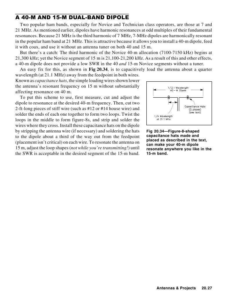
An easy fix for this, as shown in Fig 20.34, is to capacitively load the antenna about a quarterwavelength (at 21.1 MHz) away from the feedpoint in both wires.Known as capacitance hats, the simple loading wires shown lowerthe antenna’s resonant frequency on 15 m without substantiallyaffecting resonance on 40 m.
To put this scheme to use, first measure, cut and adjust thedipole to resonance at the desired 40-m frequency. Then, cut two2-ft-long pieces of stiff wire (such as #12 or #14 house wire) andsolder the ends of each one together to form two loops. Twist theloops in the middle to form figure-8s, and strip and solder thewires where they cross. Install these capacitance hats on the dipoleby stripping the antenna wire (if necessary) and soldering the hatsto the dipole about a third of the way out from the feedpoint(placement isn’t critical) on each wire. To resonate the antenna on15 m, adjust the loop shapes (not while you’re transmitting!) untilthe SWR is acceptable in the desired segment of the 15-m band.
Fig 20.34—Figure-8-shapedcapacitance hats made andplaced as described in the text,can make your 40-m dipoleresonate anywhere you like in the15-m band.

20.28 Chapter 20
! !
This antenna, first described by James Taylor, W2OZH in August 1991 QST, uses a section of the feedline as part of the antenna. Taylor’s design takes advantage of the fact that separate currents can flowon the inside and outside of the shield of a coaxial cable. Current flows from the feed- point back alongthe outside of the coax’s shield. At 1/4 λ from thefeedpoint, an RF choke effectively stops currentflow, and thus the dipole is formed.
The antenna, also known as an RFD, is shownin Fig 20.35. Dipole dimensions can be takenfrom Table 20.5. Length of coax and number ofturns for the choke are given in Table 20.7.
The RFD has the advantage of being end fed.That means no feed line supported by the an-tenna. This makes it easy to erect, and makes theRFD particularly handy for portable operation.Like any dipole, the RFD should be installed ashigh, and in the clear, as possible.
Table 20.7Choke Dimensions for RFD Antenna
Freq RG-213, RG-8 RG-583.5 22 ft, 8 turns 20 ft, 6-8 turns7 22 ft, 10 turns 15 ft, 6 turns
10 12 ft, 10 turns 10 ft, 7 turns14 10 ft, 4 turns 8 ft, 8 turns21 8 ft, 6-8 turns 6 ft, 8 turns28 6 ft, 6-8 turns 4 ft, 6-8 turns
Wind the indicated length of coaxial feed line into acoil (like a coil of rope) and secure with electrical tape.Lengths are not highly critical.
Fig 20.35—The RFD (resonant feed-line dipole) antenna for 80 m. Be sure to weatherproof thefeedpoint.

Antennas & Projects 20.29
A Simple Quad for 40 MetersMany amateurs yearn for a 40-meter antenna with more gain than a simple dipole. While two-element
rotary 40-meter beams are available commercially, they are costly and require fairly hefty rotators toturn them. This low-cost, single-direction quad is simple enough for a quick Field Day installation, butwill also make a home station very competitive on the 40-meter band.
This quad uses a 2-inch outside diameter, 18-foot boom, which should be mounted no less than 60 feethigh, preferably higher. (Performance tradeoffs with height above ground will be discussed later.) Thebasic design is derived from the N6BV 75/80-meter quad described in The ARRL Antenna Compendium,Vol 5. However, since this simplified 40-meter version is unidirectional and since it covers only oneportion of the band (CW or Phone, but not both), all the relay-switched components used in the largerdesign have been eliminated.
The layout of the simple 40-meter quad at a boom height of 70 feet is shown in Fig 20.36. The wiresfor each element are pulled out sideways from the boom with black 1/8-inch Dacron rope designedspecifically to withstand both abrasion and UV radiation. The use of the proper type of rope is veryimportant—using a cheap substitute is not a good idea. You will not enjoy trying to retrieve wires thathave become, like Charlie Brown’s kite, hopelessly entangled in nearby trees, all because a cheap rope
Fig 20.36—Layout of 40-meter quad with a boom height of 70 feet. The four stay ropes on each looppull out each loop into the desired shape. Note the 10-foot separator rope at the bottom of each loop,which helps it hold its shape. The feed line is attached to the driven element through a choke balun,consisting of 10 turns of coax in a 1-foot diameter loop. You could also use large ferrite beads overthe feed-line coax, as explained in Chapter 19. Both the driven element and reflector loops are termi-nated in SO-239 connectors tied back to (but insulated from) the tower. The reflector SO-239 has ashorted PL-259 normally installed in it. This is removed during fine-tuning of the quad, as explainedin the text.
20.30 Chapter 20
broke during a windstorm! At a boom height of 70 feet, the quad requires a “wingspread” of 140 feetfor the side ropes. This is the same wingspread needed by an inverted-V dipole at the same apex heightwith a 90° included angle between the two legs.
The shape of each loop is rather unusual, since the bottom ends of each element are brought back closeto the supporting tower. (These element ends are insulated from the tower and from each other). Havingthe elements near the tower makes fine-tuning adjustments much easier—after all, the ends of the loopwires are not 9 feet out, on the ends of the boom! The feed-point resistance with this loop configurationis close to 50 Ω, meaning that no matching network is necessary. By contrast, a more conventionaldiamond or square quad-loop configuration exhibits about a 100-Ω resistance.
Another bonus to this loop configuration is that the average height above ground is higher, leadingto a slightly lower angle of radiation for the array and less loss because the bottom of each element israised higher above lossy ground. The drawback to this unusual layout is that four more “tag-line” stayropes are necessary to pull the elements out sideways at the bottom, pulling against the 10-foot separatorropes shown in Fig 20.36.
CONSTRUCTION
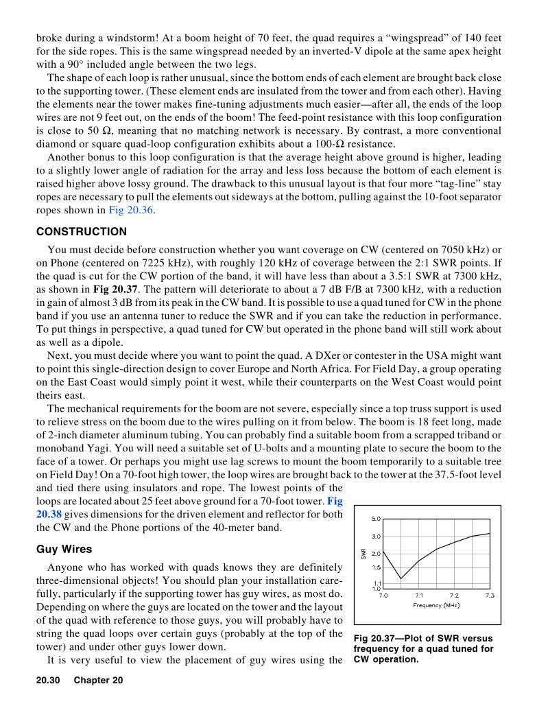
You must decide before construction whether you want coverage on CW (centered on 7050 kHz) oron Phone (centered on 7225 kHz), with roughly 120 kHz of coverage between the 2:1 SWR points. Ifthe quad is cut for the CW portion of the band, it will have less than about a 3.5:1 SWR at 7300 kHz,as shown in Fig 20.37. The pattern will deteriorate to about a 7 dB F/B at 7300 kHz, with a reductionin gain of almost 3 dB from its peak in the CW band. It is possible to use a quad tuned for CW in the phoneband if you use an antenna tuner to reduce the SWR and if you can take the reduction in performance.To put things in perspective, a quad tuned for CW but operated in the phone band will still work aboutas well as a dipole.
Next, you must decide where you want to point the quad. A DXer or contester in the USA might wantto point this single-direction design to cover Europe and North Africa. For Field Day, a group operatingon the East Coast would simply point it west, while their counterparts on the West Coast would pointtheirs east.
The mechanical requirements for the boom are not severe, especially since a top truss support is usedto relieve stress on the boom due to the wires pulling on it from below. The boom is 18 feet long, madeof 2-inch diameter aluminum tubing. You can probably find a suitable boom from a scrapped triband ormonoband Yagi. You will need a suitable set of U-bolts and a mounting plate to secure the boom to theface of a tower. Or perhaps you might use lag screws to mount the boom temporarily to a suitable treeon Field Day! On a 70-foot high tower, the loop wires are brought back to the tower at the 37.5-foot leveland tied there using insulators and rope. The lowest points of theloops are located about 25 feet above ground for a 70-foot tower. Fig20.38 gives dimensions for the driven element and reflector for boththe CW and the Phone portions of the 40-meter band.
Guy Wires
Anyone who has worked with quads knows they are definitelythree-dimensional objects! You should plan your installation care-fully, particularly if the supporting tower has guy wires, as most do.Depending on where the guys are located on the tower and the layoutof the quad with reference to those guys, you will probably have tostring the quad loops over certain guys (probably at the top of thetower) and under other guys lower down.
It is very useful to view the placement of guy wires using the
Fig 20.37—Plot of SWR versusfrequency for a quad tuned forCW operation.

Antennas & Projects 20.31
“View Antenna” function in theEZNEC modeling program.This allows you to visualize the3-D layout of an antenna. Youcan “rotate” yourself around thetower to view various aspects ofthe layout. EZNEC will com-plain about grounding wires di-rectly but will still allow you touse the View Antenna function.Note also that it is best toinsulate guy wires to prevent in-teraction between them and theantennas on a tower, but thismay not be necessary for all in-stallations.
FINE TUNING, IF NEEDED
We specify stranded #14 hard-drawn copper wire for the ele-ments. During the course of in-stallation, however, the loopwires could possibly be stretcheda small amount as you pull and
yank on them, trying to clear various obstacles. This may shift the frequency response and the performanceslightly, so it is useful to have a tuning procedure for the quad when it is finally up in the air.
The easiest way to fine-tune the quad while on the tower is to use a portable, battery-operated SWRindicator (such as the Autek RF-1 or the MFJ-259) to adjust the reflector and the driven element lengthsfor specific resonant frequencies. You can eliminate the influence of mutual coupling to the otherelement by open-circuiting the other element.
For convenience, each quad loop should be connected to an SO-239 UHF female connector that isinsulated from but tied close to the tower. You measure the driven element’s resonant frequency by firstremoving the shorted PL-259 normally inserted into the reflector connector. Similarly, the reflector’sresonant frequency can be determined by removing the feed line normally connected to the drivenelement’s feed point.
Obviously, it’s easiest if you start out with extra wire for each loop, perhaps 6 inches extra on eachside of the SO-239. You can then cut off wire in 1/2-inch segments equally on each side of the connector.This procedure is easier than trying to splice extra wire while up on the tower. Alligator clips are usefulduring this procedure, but just don’t lose your hold on the wires! You should tie safety strings from eachwire back to the tower. Prune the wire lengths to yield the resonant frequencies (±5 kHz) shown inFig 20.38 and then solder things securely. Don’t forget to reinsert the shorted PL-259 into the reflectorSO-239 connector to turn it back into a reflector.
HIGHER IS BETTER
This quad was designed to operate with the boom at least 60 feet high. However, it will workconsiderably better for DX work if you can put the boom up even higher. Fig 20.39 shows the elevationpatterns for four antennas: a reference inverted-V dipole at 70 feet (with a 90° included angle betweenthe two legs), and three quads, with boom height of 70, 90 and 100 feet respectively. At an elevation angle
Fig 20.38—Dimensions of each loop, for CW or Phone operation.
7050 kHz, 7200 kHz,
CW SSBLength A, Reflector 31'6'' 30'103/4''Length B, Reflector 28'21/4'' 27'7''Length C, Reflector 15'71/4'' 15'Total, Half Reflector 75'31/2'' 73'53/4''Resonant Frequency 7030 kHz 7205 kHzLength A, Driven 30'71/4'' 30'Length B, Driven 27'31/2'' 26'81/2''Length C, Driven 14'71/2'' 14'Length, Half Driven 72'61/4'' 70'81/2''Self-Resonant Frequency 7295 kHz 7480 kHz

20.32 Chapter 20
of 20°, typical for DX work on40 meters, the quad at 100 feethas about a 5 dB advantageover an inverted-V dipole at 70feet, and about a 3 dB advan-tage over a quad with a boomheight of 70 feet.
Fig 20.39—Comparisons of the elevation patterns for quads atboom heights of 70, 90 and 100 feet, referenced to an inverted-Vdipole at 70 feet.

Antennas & Projects 20.33
Vertical AntennasOne of the more popular amateur antennas is the vertical. Although amateurs often use the term
“vertical” somewhat loosely, it usually refers to a single radiating element placed vertically over theground. A vertical is usually 1/4-λ long electrically and constructed out of wire or tubing. Many amateurslive on city lots with zoning restrictions preventing them from putting up tall towers with large Yagiarrays. Amateurs are also creative and ingenious—a vertical disguised to look like a flagpole can be bothpatriotic and a good radiator of RF!
Vertical antennas are omnidirectional radiators. This can be beneficial or detrimental, depending onthe exact situation. On transmission there are no nulls in any direction, unlike most horizontal antennas.However, QRM on receive can’t be nulled out from the directions that are not of interest, unless multipleverticals are used in an array.
When compared to horizontal antennas, verticals also suffer more acutely from two main types oflosses—ground return losses for currents in the near field, and far-field ground losses. Ground lossesin the near field can be minimized by using many ground radials. This is covered in detail in the followingsection.
Far-field losses are highly dependent on the conductivity and dielectric constant of the earth around theantenna, extending out as far as 100 λ from the base of the antenna. There is very little that someone cando to change the character of the ground that far away—other than moving to a small island surroundedby saltwater! Far-field losses greatly affect low-angle radiation, causing the radiation patterns of practicalvertical antennas to fall far short of theoretical patterns over “perfect ground,” often seen in classical texts.Fig 20.41 shows the elevation pattern response for two different 40-m quarter-wave verticals. One isplaced over a theoretical infinitely large, infinitely conducting ground. The second is placed over anextensive radial system over average soil, having a conductivity of 5 mS/m and a dielectric constant of 13.This sort of soil is typical of heavy clay found in pastoral regions of the US mid-Atlantic states. At a 10°elevation angle, the real antenna losses are almost 6 dB compared to the theoretical one; at 20° the differ-ence is about 3 dB. See The ARRL Antenna Book chapter on the effects of the earth for further details.
While real verticals over real ground are not a magic method to achieve low-angle radiation, costversus performance and ease ofinstallation are incentives thatinspire many antenna builders.For use on the lower frequencyamateur bands—notably 160and 80 m—it is not always prac-tical to erect a full-size vertical.At 1.8 MHz, a full-sized quar-ter-wave vertical is 130 ft high.In such instances it is often nec-essary to accept a shorter radiat-ing element and use some formof loading.
Fig 20.42 provides curves forthe physical height of verticals inwavelength versus radiation re-sistance and reactance. Althoughthe plots are based on perfectlyconducting ground, they showgeneral trends for installations
Fig 20.41—Elevation patternsfor two quarter-wave verticalantennas over different ground.One vertical is placed over“perfect” ground, and the otheris placed over average ground.The far-field response at lowelevation angles is greatlyaffected by the quality of theground—as far as 100 λλλλλ awayfrom the vertical antenna.
Fig 20.42—Radiation resistance(solid curve) and reactance(dotted curve) of vertical anten-nas as a function of physicalheight.

20.34 Chapter 20
where many radials have been laid out to make a ground screen. As the radiator is made shorter, the radiationresistance decreases—with 6 Ω being typical for a 0.1-λ high antenna. The lower the radiation resistance, themore the antenna efficiency depends on ground conductivity and the effectiveness of the ground screen. Also,the bandwidth decreases markedly as the length is reduced toward the left of the scale in Fig 20.42. It can bedifficult to develop suitable matching networks when radiation resistance is very low.
Ground Systems
The importance of an effective ground system for vertical antennas cannot be emphasized too strongly.However, it is not always possible to install a radial network that approaches the ideal. The AM broadcastindustry uses 120 buried radials as a standard radial ground system for their antennas. This is rarelypractical for most amateurs, and a compromise ground is certainly better than no ground at all. Theamateur should experiment with whatever is physically possible when working with vertical antennas.Even modest radial systems can produce contacts, even if they don’t consistently crack big pileups!
Although the matter of less-than-optimum ground systems could be debated almost endlessly, somepractical rules of thumb are in order for those wishing to erect vertical antennas. Generally a largenumber of shorter radials offers a better ground system than a few longer ones. For example, 8 radialsof 1/8 λ are preferred over 4 radials of 1/4 λ. If the physical height of the vertical is an 1/8 λ, the radial wiresshould be of the same length and dispersed uniformly from the base.
The conductor size of the radials is not especially significant. Wire gauges from #4 to #20 have beenused successfully by amateurs. Copper wire is preferred, but where soil is low in acid (alkali), aluminumwire can be used. The wires may be bare or insulated, and they can be laid on the earth’s surface or burieda few inches below ground. Insulated wires will have greater longevity by virtue of reduced corrosionand dissolution from soil chemicals. The amateur should bury as much ground wire as time and budgetpermit. Some operators have literally miles of wire buried radially beneath their vertical antennas.
When property dimensions do not allow a classic installation of equally spaced radial wires, they canbe placed on the ground as space permits. They may run away from the antenna in only one or twocompass directions. They may be bent to fit on your property.
A single ground rod, or group of them bonded together, is seldom as effective as a collection ofrandom-length radial wires. In some instances a group of short radial wires can be used in combinationwith ground rods driven into the soil near the base of the antenna. Bear in mind, though, that RF currentsat MF and HF seldom penetrate the earth more than several inches. If a metal fence skirts the propertyit can be used as part of the ground system. Rolls of galvanized “chicken wire” fencing fanned out fromthe base of the vertical make good ground systems, especially when used in conjunction with longer wireradials. Six 30-ft long by 3-ft wide rolls of chicken wire make a good ground screen for a 160-m vertical,backed up with 6 or more 130-ft long radials. A good rule is to use anything that will serve as a groundwhen developing a radial ground system.
All radial wires should be connected together at the base of the vertical antenna. The electrical bondneeds to be of low resistance. Best results will be obtained when the wires (and chicken-wire screen, ifused) are soldered together at the junction point. When a grounded vertical is used, the ground wiresshould be affixed securely to the base of the driven element. A lawn edging tool is excellent for cuttingslits in grass sod or in soil when laying radial wires.
Ground return losses are lower when vertical antennas and their radials are elevated above ground,a point that is well-known by those using ground plane antennas on their roofs. Even on 160 or 80 m,effective vertical antenna systems can be made with as few as four quarter-wave long radials elevated10 to 20 ft off the ground.
Full-Size Vertical Antennas
When it is practical to erect a full-size l/4 λ vertical antenna, the forms shown in Fig 20.43 are worthy

Antennas & Projects 20.35
of consideration. The exampleat A is the well-known verticalground plane. The ground sys-tem consists of four above-ground radial wires. The lengthof the radials and the drivenelement is derived from thestandard equation
f(MHz)234
= (ft) L (6)
With four equidistant radialwires drooped at approxi-mately 45° (Fig 20.43A), thef e e d - p o i n t i m p e d a n c e i sroughly 50 Ω. When the radi-als are at right angles to theradiator (Fig 20.43B) the im-pedance approaches 36 Ω. Be-sides minimizing ground returnlosses, another major advan-tage in this type of vertical an-tenna over a ground-mountedtype is that the system can beelevated well above nearby
conductive objects (power lines, trees, buildings and so on). When drooping radials are used, they canalso serve as guy wires for the mast that supports the antenna. The coax shield braid is connected to theradials, and the center conductor to the driven element.
The Marconi vertical antenna shown in Fig 20.43C is the classic form taken by a ground-mountedvertical. It can be grounded at the base and shunt fed, or it can be isolated from ground, as shown, andseries fed. As always, this vertical antenna depends on an effective ground system for efficient perfor-mance. If a perfect ground were located below the antenna, the feed impedance would be near 36 Ω. Ina practical case, owing to imperfect ground, the impedance is more apt to be in the vicinity of 50 to 75 Ω.
A gamma feed system for a grounded 1/4-λ vertical is presented in Fig 20.43D. Some rules of thumbfor arriving at workable gamma-arm and capacitor dimensions are to make the rod length 0.04 to 0.05 λ,its diameter 1/3 to 1/2 that of the driven element and the center-to-center spacing between the gamma armand the driven element roughly 0.007 λ. The capacitance of C1 at a 50-Ω matched condition will be about7 pF per meter of wavelength. The absolute value of C1 will depend on whether the vertical is resonantand on the precise value of the radiation resistance. For best results, make the radiator approximately3% shorter than the resonant length.
Amateur antenna towers lend themselves to use as shunt-fed verticals, even though an HF-band beamantenna is usually mounted on the tower. The overall system should be close to resonance at the desiredoperating frequency if a gamma feed is used. The HF-band beam will contribute somewhat to top loadingof the tower. The natural resonance of such a system can be checked by dropping a #12 or #14 wire fromthe top of the tower (making it common to the tower top) to form a folded unipole (Fig 20.43E). A four-or five-turn link can be inserted between the lower end of the drop wire and the ground system. A dipmeter is then inserted in the link to determine the resonant frequency. If the tower is equipped with guywires, they should be broken up with strain insulators to prevent unwanted loading of the vertical. In such
Fig 20.43—Various types of vertical antennas.

20.36 Chapter 20
cases where the tower and beam antennas are not able to provide 1/4-λ resonance, portions of the top guywires can be used as top-loading capacitance. Experiment with the guy-wire lengths (using the dip-metertechnique) while determining the proper dimensions.
A folded-unipole is depicted at E of Fig 20.43. This system has the advantage of increased feed-pointimpedance. Furthermore, a Transmatch can be connected between the bottom of the drop wire and theground system to permit operation on more than one band. For example, if the tower is resonant on 80 m,it can be used as shown on 160 and 40 m with reasonable results, even though it is not electrically longenough on 160. The drop wire need not be a specific distance from the tower, but you might try spacingsbetween 12 and 30 inches.
The method of feed shown at Fig 20.43F is commonly referred to as “slant-wire feed.” The guy wiresand the tower combine to provide quarter-wave resonance. A matching network is placed between thelower end of one guy wire and ground and adjusted for an SWR of 1:1. It does not matter at which levelon the tower the guy wires are connected, assuming that the Transmatch is capable of effecting a matchto 50 Ω.
Physically Short Verticals
A group of short vertical radiators is presented in Fig 20.44. Illustrations A and B are for top and centerloading. A capacitance hat is shown in each example. The hat should be as large as practical to increasethe radiation resistance of the antenna and improve the bandwidth. The wire in the loading coil is chosenfor the largest gauge consistent with ease of winding and coil-form size. The larger wire diameters willreduce the resistive (I2R) losses in the system. The coil-form material should have a medium or highdielectric constant. Phenolic orfiberglass tubing is entirely ad-equate.
A base-loaded vertical isshown at C of Fig 20.44. Theprimary limitation is that thehigh current portion of the ver-tical exists in the coil ratherthan the driven element. Withcenter loading, the portion ofthe antenna below the coil car-ries high current, and in the top-loaded version the entire verti-cal element carries highcurrent. Since the high-currentpart of the antenna is respon-sible for most of the radiating,base loading is the least effec-tive of the three methods. Theradiation resistance of the coil-loaded antennas shown is usu-ally less than 16 Ω.
A method for using guywires to top load a short verti-cal is illustrated in Fig 20.44D.This system works well withgamma feed. The loading wires
Fig 20.44—Vertical antennas that are less than one-quarter wave-length in height.

Antennas & Projects 20.37
are trimmed to provide an electrical quarter wavelength for the overall system. This method of loadingwill result in a higher radiation resistance and greater bandwidth than the systems shown at A throughC. If an HF-band or VHF array is at the top the tower, it will simply contribute to the top loading.
A three-wire unipole is shown at E. Two #8 drop wires are connected to the top of the tower andbrought to ground level. The wires can be spaced any convenient distance from the tower—normally 12to 30 inches from one side. C1 is adjusted for best SWR. This type of vertical has a fairly narrowbandwidth, but because C1 can be motor driven and controlled from the operating position, frequencychanges can be accomplished easily. This technique will not be suitable for matching to 50-Ω line unlessthe tower is less than an electrical quarter wavelength high.
A different method for top loading is shown at F. Barry Boothe, W9UCW, described this method inDecember 1974 QST. An extension is used at the top of the tower to effect an electrical quarter-wavelength vertical. L1 is a loading coil with sufficient inductance to provide antenna resonance. Thistype of antenna lends itself nicely to operation on 160 m.
A method for constructing the top-loading shown in Fig 20.44F is illustrated in Fig 20.45. Pipesection D is mated with the mast above the HF-band beam antenna. A loading coil is wound on solidPlexiglas rod or phenolic rod (item C), then clamped inside the collet (B). An aluminum slug (part A)is clamped inside item B. The top part of A is bored and tapped for a 3/8 × 24 stud. This permits a standard8-ft stainless-steel mobile whip to be threaded into item A above the loading coil. The capacitance hat(Fig 20.45B) can be made from a 1/4-inch-thick brass or aluminum plate. It may be round or square.Lengths of 1/8-inch brazing rod can be threaded and screwed into the edge of the aluminum plate. Theplate contains a row of holes along its perimeter, each having been tapped for a 6-32 thread. Thecapacitance hat is affixed to item A by means of the 8-ft whip antenna. The whip will increase theeffective height of the verticalantenna.
Cables and Control Wires onTowers
Most vertical antennas of thetype shown in Fig 20.43 con-sist of towers, usually with HFor VHF beam antennas at thetop. The rotator control wiresand the coaxial feeders to thetop of the tower will not affectantenna performance ad-versely. In fact, they become apart of the composite antenna.To prevent unwanted RF cur-rents from following the wiresinto the shack, simply dressthem close to the tower legs andbring them to ground level.This decouples the wires at RF.The wires should then berouted along the earth surface(or buried underground) to theoperating position. It is not nec-essary to use bypass capacitors
Fig 20.45—At A are the details for the tubing section of the loadingassembly. Illustration B shows the top hat and its spokes. Thelonger the spokes, the better.

20.38 Chapter 20
or RF chokes in the rotator control leads if this is done, even whenmaximum legal power is employed.
Trap Verticals
The 2-band trap vertical antenna of Fig 20.46 operates in much thesame manner as a trap dipole or trap Yagi. The notable difference isthat the vertical is one half of a dipole. The radial system (in-groundor above-ground) functions as a ground plane for the antenna, andrepresents the missing half of the dipole. Once again, the more effec-tive the ground system, the better will be the antenna performance.
Trap verticals usually are adjusted as 1/4-λ radiators. The portion ofthe antenna below the trap is adjusted as a 1/4-λ radiator at the higherproposed operating frequency. That is, a 20/15-m trap vertical wouldbe a resonant quarter wavelength at 15 m from the feedpoint to thebottom of the trap. The trap and that portion of the antenna above thetrap (plus the 15-m section below the trap) constitute the completeantenna during 20-m operation. But because the trap is in the circuit,the overall physical length of the vertical antenna will be slightly lessthan that of a single-band, full-size 20-m vertical.
Traps
The trap functions as the name implies: It traps the 15-m energyand confines it to the part of the antenna below the trap. During 20-m operation it allows the RF energy to reach all of the antenna. Thetrap in this example is tuned as a parallel resonant circuit to 21 MHz.At this frequency it divorces the top section of the vertical from thelower section because it presents a high impedance (barrier) at21 MHz. Generally, the trap inductor and capacitor have a reactanceof 100 to 300 Ω. Within that range it is not critical.
The trap is built and adjusted separately from the antenna. Itshould be resonated at the center of the portion of the band to beoperated. Thus, if one’s favorite part of the 15-m band is between21.0 and 21.1 MHz, the trap should be tuned to 21.05 MHz.
Resonance is checked by using a dip meter and detecting the dipper signal in a calibrated receiver.Once the trap is adjusted it can be installed in the antenna, and no further adjustment will be required.It is easy, however, to be misled after the system is assembled: Attempts to check the trap with a dip meterwill suggest that the trap has moved much lower in frequency (approximately 5 MHz lower in a 20/15-m vertical). This is because the trap is part of the overall antenna, and the resultant resonance is that ofthe total antenna. Measure the trap separate from the rest of the antenna.
Multiband operation is quite practical by using the appropriate number of traps and tubing sections.The construction and adjustment procedure is the same, regardless of the number of bands covered. Thehighest frequency trap is always closest to the feed end of the antenna, and the next to lowest frequencytrap is always the farthest from the feedpoint. As the operating frequency is progressively lowered, moretraps and more tubing sections become a functional part of the antenna.
Traps should be weatherproofed to prevent moisture from detuning them. Several coatings of highdielectric compound, such as Polystyrene Q Dope, are effective. Alternatively, a protective sleeve ofheat-shrink tubing can be applied to the coil after completion. The coil form for the trap should be ofhigh dielectric quality and be rugged enough to sustain stress during periods of wind.
Fig 20.46—A two-band trapvertical antenna. The trapshould be resonated by itself asa parallel resonant circuit at thecenter of the operating range forthe higher frequency band. Thereactance of either the inductoror the capacitor range from 100to 300 ΩΩΩΩΩ. At the lower frequencythe trap will act as a loadinginductor, adding electricallength to the total antenna.

Antennas & Projects 20.39
&! " # 1 2 ##
Driving a ground rod 8 feet into the ground with a sledgehammer batters the rod end into an uglyflare. Some types of ground clamps can’t open far enough to slip over the enlarged rod. Of course,you can file, grind or saw off the flared end, but doing all of these things at ground level can bedifficult.
Alternatively, you could slip the clamp over the rod before driving it into the ground; or use a clampthat opens far enough to pass over the flare. In the case of1/2-inch ground rods, however, clamps wide enough to pass the flare may not tighten adequately.
After considering these problems, I attached my shack ground wire to a 1/2-inch ground rod asfollows. I drilled a tap-size hole, about 3/4 inch deep, into the rod top. I tapped this hole for a 1/4-inch,standard thread. Driving in a hex-head bolt permitted firm attachment of the wire to the rod end.
Although I did this by drilling only one hole, drilling a pilot hole—say, about 1/8 inch in diameter—before driving in the rod would assist. Doing so would allow you to put the rod in a vise for stabilityand accurate drilling. Your sledgehammer may obliterate this hole, but you should be able to relocateit by probing with a center punch.
In any such drilling and thread cutting, use a sharp drill and lubricate it and your tap often whilecutting. One more tip: If you have a welder friend, consider having him or her weld a 1/4-inch bolt tothe ground-rod top—after you’ve driven it in—to provide a stud for connections.—A. W. Edwards,K5CN, Corpus Christi, Texas

20.40 Chapter 20
3!45()!65)-
Thanks to the harmonic relationships between the HF ham bands, many antennas can be made to do“double duty.” The simple verticals described here cover two bands at once. Here’s how to turn a30-m 1/4-λ vertical into a 0.625-λ vertical for the 12-m band, and a 40-m 1/4-λ vertical into a 0.625-λvertical for the 17-m band. These verticals were designed and constructed by John J. Reh, K7KGP. Thewrite-up first appeared in April 1989 QST.
Construction Details
For the 30 and 12-m vertical, an old aluminum multiband vertical was cut to a length of 25 ft, 3 inches.This corresponds to a design frequency of 24.95 MHz. The length-to-diameter ratio is approximately460. The input impedance of a vertical that is substantially longer than a 1/4-λ (in this case 0.625 λ) isparticularly sensitive to the λ/D ratio of the radiating element. If this antenna is duplicated with materialshaving a significantly different λ/D ratio, the results may be different.
After installing a good ground system, the input impedance was measured and found to have aresistance of about 50 Ω, and a capacitance of about –155 Ω (at 24.95 MHz). At 10.125 MHz, the inputimpedance was just under 50 Ω, and purely resistive. To tune out the reactance at 24.95 MHz, a seriesinductor is installed (see Fig 20.47) and tapped to resonance at the design frequency. The easiest wayto find resonance is by measuring the antenna SWR. Use a good-quality coil for the series inductor. Therecommended coil has a diameter of 21/2 inches, and has 6 turns per inch (B&W stock no. 3029).Resonance on 12 m was established with 31/4 turns. The SWR on 12 m is 1.1:1, and on 30 m, 1:1. Tochange bands from 12 to 30 m, move the coil tap to the end of thecoil closest to the vertical element. Alternatively, a single-poleswitch or remotely operated relay can be installed at the base of thevertical for bandswitching.
The Ground System
Maximum RF current density—and therefore maximum groundlosses—for 1/4-λ verticals occurs in the immediate area of thebase of the antenna. Maximum return current ground loss for a0.625-λ vertical occurs about 1/2 λ away from the base of theantenna. It’s important to have the lowest possible losses in theimmediate area for both types of verticals. In addition to a groundradial system, 6×6-ft aluminum ground screen is used at the baseof the antenna. The screen makes a good tie point for the radialsand conducts ground currents efficiently. Seventeen wire radials,each about 33 ft long, are spaced evenly around the antenna. Moreradials would probably work better. Each radial is bolted to thescreen using corrosion-resistant #10-24 hardware. (Do not attemptto connect copper directly to aluminum. The electrical connectionbetween the two metals will quickly deteriorate.) The radials canbe made of bare or insulated wire. Make sure the ground screen isbolted to the ground side of the antenna with heavy-gauge wire.Current flow is fairly heavy at this point.
Table 20.8 gives specifications for the dual-band vertical. Ifyour existing 40-m vertical is a few inches longer than 32 ft,3 inches, try using it anyway—a few inches isn’t too critical toperformance on 17 m.
Fig 20.47—Dual-band vertical.Use a switch or relay to removethe loading coil from the circuitfor lower frequency operation.Adjust the coil tap for best SWRon the higher-frequency band.The radial system should be asextensive as possible. See TheARRL Antenna Book for moreinformation on ground systemsfor vertical antennas.

Antennas & Projects 20.41
Automatic Bandswitching
In October 1989 QST, James Johnson,W8EUI, presented this scheme for automaticbandswitching of the 40/17-m vertical. Johnsonshortened his 40-m vertical approximately12 inches and found an inductance that gave him40 and 17-m band operation with an SWR of lessthan 1.4:1 across each band. He used an inductor
made from B&W air-wound coil stock (no. 3033). This coil is 3 inches in diameter, and has 31/8 turnsof #12 wire wound at 6 turns per inch, providing an inductance of about 2.8 µH. Johnson experimentallydetermined the correct tap position.
For the 30/12-m version, start with the vertical radiator 9 inches shorter than the value given in thetable. In both cases, radiator height and inductance should be adjusted for optimum match on the twobands covered.
Table 20.8Specifications for Dual-Band Verticals
Required MatchingBands Height Inductance (µH)12 m & 30 m 23' 5" 0.9917 m & 40 m 32' 3" 1.36

20.42 Chapter 20
# 7"! 31" "
" %
A vertical antenna can induce current on the shield of its coax feeder. The antenna induces currenton the shield in the same manner that it induces current in the ground-system radials.
Since the shield is connected to station ground, RF current flowing on the feeder shield also flowson the outer surfaces of the equipment when the transmitter operates. This current can induce unde-sirable voltages in interconnecting cables, causing erratic operation of computer keyboards andpower supplies. RF feedback also can occur through the transmitter microphone circuit.
These problems occurred when I operated my kilowatt power amplifier and Kenwood TS-940Stransceiver. (RF feedback in the TS-940 microphone preamplifier has been recognized by others andcan be solved with bypass capacitors and RF chokes.) A better solution—one that will address allstation problems caused by coax-shield RF currents—is to prevent the RF from getting into thestation from the coax shield. Gary Peterson, K0CX, suggested that I do this by putting a ferrite-beadshield-current choke in my antenna feed line where it enters my station.
A good source of the required components is The Wireman, Inc (see Address List in References).The required components are a package of 50 type FB73-2401 ferrite beads (Wireman part #912B),15 inches of RG-303 coax, and two coax connectors (UHF connectors [PL-259s; the Wireman’s #702]with inserts [UG-175s; the Wireman’s #704] for installation on RG-58 coax, or N connectors intendedfor installation on RG-58 [UG-536B/Us, available as the Wireman’s #737). Although the Wiremansells these parts bundled as part of a W2DU Balun kit [#833], the coax in the kit is too short to accom-modate the connectors, so I recommend ordering the parts individually instead of buying them as TheWireman’s W2DU Balun kit.
To assemble the choke, install one connector on the cable. Because the UG-536B/U connector ismade for RG-58 (which has a larger diameter than RG-303), you must heat-shrink a piece of 1-inch-long, 3/16-inch-diameter plastic tubing on the end of the coax before you install the connector. This willmake the connector fit the cable tightly.
Next, put a 1/2-inch-long piece of heat-shrink tubing on the cable about 1 inch from the connector tohold the beads in place. Then place the 50 beads on the cable. Put on another 1/2-inch piece of tubingto anchor the other end of the beads, and then shrink a piece of 3/8-inch-diameter tubing over thebeads. Install the other connector on the cable. Install the choke on the transmission line where itleaves your station.
This should largely do away with problems related to stray RF traveling into your station on yourfeed line’s coax shield. An idea for clubs: Build one or more chokes that members can borrow to testthis fix’s effectiveness before building their own chokes.
If your station is not in the immediate vicinity of your antenna and you have problems with stray RFwith a dipole or inverted V, the problem may be due to lack of a balun or use of an ineffective balun. Ifthis is the case, install the choke at the antenna feedpoint as discussed in W2DU's book Reflectionsrather than using the choke at the station end of your feed line.—Bruce R. Palmer, K0WM, Edmond,Oklahoma

Antennas & Projects 20.43
!/2!
A tree-mounted, vertically polarized antenna may sound silly. But is it, really? Perhaps engineeringreferences do not recommend it, but such an antenna does not cost much, is inconspicuous, and it works.This idea was described by Chuck Hutchinson, K8CH, in QST for September 1984.
The antenna itself is simple, as shown in Fig 20.48. A piece of RG-58 cable runs to the feedpoint ofthe antenna, and is attached to a porcelain insulator. Two radial wires are soldered to the coax-line braidat this point. Another piece of wire forms the radiator. The top of the radiator section is suspended froma tree limb or other convenient support, and in turn supports the rest of the antenna.
The dimensions for the antenna are given in Fig 20.49. (You can use the values given for leg lengthsin Table 20.5.) All three wires of the antenna are 1/4-λ long. This generally limits the usefulness of theantenna for portable operation to 7 MHz and higher bands, as temporary supports higher than 35 or 40 ftare difficult to come by. Satisfactory operation can be accomplished on 3.5 MHz with an inverted-Lconfiguration of the radiator, if you can overcome the accompanying difficulty of erecting the antennaat the operating site. The tree-mounted vertical idea can also be used for fixed station installations tomake an “invisible” antenna. Shallow trenches can be slit for burying the coax feeder and the radialwires. The radiator itself is difficult to see unless you are standing right next to the tree.
Fig 20.48—The feedpoint of thetree-mounted groundplaneantenna. The opposite ends ofthe two radial wires may beconnected to stakes or otherconvenient anchor points. Makesure that the radials are highenough so that people cannotcome in contact with them.
Fig 20.49—Dimensions and construction of the tree-mountedgroundplane antenna.

20.44 Chapter 20
Inverted L and Sloper AntennasThis section covers varia-
tions on the vertical antenna.Fig 20.50A shows a flat-top Tvertical. Dimension H shouldbe as tall as possible for bestresults. The horizontal section,L, is adjusted to a length thatprovides resonance. Maximumradiation is polarized verticallydespite the horizontal top-load-ing wire. A variation of the Tantenna is depicted at B ofFig 20.50. This antenna is com-monly referred to as an invertedL. Vertical member H shouldbe as long as possible. L isadded to provide an electricalquarter wavelength overall.
Fig 20.50—Some variations in vertical antennas. D is the verticalradiation pattern in the plane of a half sloper, with the sloper to theright. E is the azimuthal pattern of the half sloper (90° azimuth isthe direction of the sloping wire). Both patterns apply to 160- and80-m antennas described in the text.

Antennas & Projects 20.45
//!
Many hams have had excellent results with half-sloper antennas, while others have not had such luck.Work by ARRL Technical Advisor John S. Belrose, VE2CV, has brought some insight to the situationthrough computer modeling with ELNEC and antenna-range tests. The following is taken from VE2CV’sTechnical Correspondence in Feb 1991 QST, pp 39 and 40. Essentially, the half sloper is a top-fedvertical antenna worked against a ground plane (such as a grounded Yagi antenna) at the top of the tower.The tower acts as a reflector.
For half slopers, the input impedance, the resonant length of the sloping wire and the antenna patternall depend on the tower height, the angle (between the sloper and tower) the type of Yagi and the Yagiorientation. Here are several configurations extracted from VE2CV’s work:
At 160 m—use a 40-m beam on top of a 95-ft tower with a 55° sloper apex angle. The radiation patternvaries little with Yagi type. The pattern is slightly cardioid with about 8 dB front-to-back ratio at a 25ºtakeoff angle (see Fig 20.50D and E). Input impedance is about 50 Ω.
At 80 m—use a 20-m beam on top of a 50-ft tower with a 55° sloper apex angle. The radiation patternand input impedance are similar to those of the 160-m half sloper.
At 40 m—use a 20-m beam on top of a 50-ft tower with a 55° sloper apex angle. The radiation patternand impedance depend strongly on the azimuth orientation of the Yagi. Impedance varies from 76 to127 Ω depending on Yagi direction.

20.46 Chapter 20
8+/93
The antenna shown in Fig20.51 is simple and easy to con-struct. It is a good antenna forthe beginner or the experienced1.8 MHz DXer. Because theoverall electrical length isgreater than 1/4 λ, the feed-point resistance is on the orderof 50 Ω, with an inductive re-actance. That reactance is can-celed by a series capacitor,which for power levels up tothe legal limit can be a air-vari-able capacitor with a voltagerating of 1500 V. Adjust an-tenna length and variable ca-pacitor for lowest SWR.
A yardarm or a length of lineattached to a tower can be usedto support the vertical sectionof the antenna. (Keep the in-verted L as far from the toweras is practical. Certain combinations of tower height and Yagi top loading can interact severely with theInverted-L antenna—a 70-ft tower and a 5-element Yagi, for example.) For best results the verticalsection should be as long as possible. A good ground system is necessary for good results.
Fig 20.51—The 1.8-MHz inverted L. Overall wire length is 165 to175 ft. The variable capacitor has a maximum capacitance of 500to 800 pF.

Antennas & Projects 20.47
/,3
In July 1991 QST, Dennis Monticelli, AE6C, described a dual-band inverted L. A drawing of hisinstallation is shown in Fig 20.52. Dimensions and values are given in Table 20.9. For ease ofexplanation, only the 80/40-mversion is described here. On80 m the antenna is 0.375 λlong, which raises theantenna’s radiation resistanceand feed-point impedance,and thus decreases the effectof ground losses. (The feed-point exhibits inductive reac-tance—which is canceled withseries capacitance.) For 40 mthe antenna is 0.75 λ long, andis therefore resonant on thatband. The pattern on 40 m, de-pending on how you install theantenna, resembles a combi-nation of a vertical and a lowdipole.
If you use a modest radial sys-tem with this antenna, the feed-point impedance is roughly100 Ω on both bands. Fig 20.53and Fig 20.54 show details ofthe matching system and the 1:2(50 to 100 Ω) broadband trans-former. The matching capaci-
Fig 20.52—Drawing of the Dual-Band Inverted-L antenna installedat AE6C.
Table 20.9Recommended Wire Lengths and Capacitor Values*
Bands Vertical Horizontal Total SeriesLength (ft) Length (ft) Length (ft) Capacitor
80/40 32 64 96 ≈ 100 pF160/80 64 128 192 ≈ 200 pF
* The total length is important, but the portions allocated to the verticaland horizontal members aren’t critical.
Fig 20.53—The resonating, impedance-matching,and band-switching circuitry required at thebase of the inverted L. Fig 20.54 shows detailsof T1.
Fig 20.54—Winding details for constructingbroadband bifilar transformer T1, which iswound on T-200-2 core. The primary is 16 turnsof #14 enameled wire, and the secondary is 10turns of #14 enameled wire tapped at about theeighth turn from the feed-line end.

20.48 Chapter 20
tor, C1, is not used on the higher frequency band,and so it is shorted out to operate there.
To tune the antenna, start with the dimensionsgiven in Table 20.9. With the series capacitorshorted, trim the wire length for best SWR atyour 40-m frequency of interest. Unshort thecapacitor and adjust it for best SWR at your fre-quency of interest on 80 m. You can further ad-just SWR by changing transformer taps. (Thiswill affect both bands.) As shown in Fig 20.55,a single capacitance value yields a 2:1 SWRbandwidth of approximately 225 kHz on 80 m.Different capacitance values can be used to coverother parts of the 80-m band.
You can make you own fixed-value, high-voltage, high-current capacitor from a piece ofcoax. For example, RG-8 (solid dielectric) ex-hibits 29.5 pF per ft and can withstand 4 kV atseveral amperes. Connect it by attaching one endof the inner conductor to the antenna and thebraid (at the same end) to the feed system; leavethe other end open. Start with about 4 ft of RG-8 and trim the coax for minimum SWR. (Makeyour cuts when you’re not transmitting!) Othersolid-dielectric cables are also suitable for thisapplication. The Transmission Lines chaptergives capacitance per unit length in its table ofcoaxial-cable characteristics. The ends of thecoaxial capacitors must be sealed to preventwater ingress.
7:!6; 1<
Those little red plastic caps (CAPLUGS) that are used to protectunused coax (SO-239) connectors from moisture, dirt and damageare expensive if you are lucky enough to find them. An alternativeis to use plastic caps from inexpensive champagne bottles (Fig A).These caps fit perfectly.—Roy Berkowitz, K3NFU, Monroeton,Pennsylvania
Fig A—Champagne corks maybe recycled into protectivecaps for SO-239 connectors.
Fig 20.55—At A, 40-m SWR curve. At B, measuredSWR curves for 80 m. Curves representing twodifferent series capacitor values are shown.

Antennas & Projects 20.49
*3*32!
This article describes a simple and effective means of using a grounded tower, with or without top-mounted antennas, as an elevated ground-plane antenna for 80 and 160 m. It first appeared in a June 1994QST article by Thomas Russell, N4KG.
FROM SLOPER TO VERTICAL
Recall the quarter-wavelength sloper, also known as the half-sloper. It consists of an isolated quarterwavelength of wire, sloping from an elevated feedpoint on a grounded tower. Best results were usuallyobtained when the feedpoint was somewhere below a top-mounted Yagi antenna. You feed a sloper byattaching the center conductor of a coaxial cable to the sloping wire and the braid of the cable to the towerleg. Now, imagine four (or more) slopers, but instead of feeding each individually, connect themtogether to the center conductor of a single feed line. Voilà! Instant elevated ground plane.
Now, all you need to do is determine how to tune the antenna to resonance. With no antennas on thetop of the tower, the tower can be thought of as a fat conductor and should be approximately 4% shorterthan a quarter wavelength in free space. Calculate this length and attach four insulated quarter-wave-length radials at this distance from the top of the tower. For 80 m, a feedpoint 65 ft below the top of anunloaded tower is called for. The tower guys must be broken up with insulators for all such installations.For 160 m, 130 ft of tower above the feedpoint is needed.
What can be done with a typical grounded-tower-and-Yagi installation? A top-mounted Yagi acts asa large capacitance hat, top loading the tower. Fortunately, top loading is the most efficient means ofloading a vertical antenna.
The examples in Fig 20.56 should give us an idea of how much top loading might be expected fromtypical amateur antennas. The values along the horizontal axis tell us the approximate vertical heightreplaced by the antennas listed in a top-loaded vertical antenna. To arrive at the remaining amount oftower needed for resonance, subtract these numbers from the nonloaded tower height needed for reso-nance. Note that for all but the 10-m antennas, the equivalent loading equals or exceeds a quarterwavelength on 40 m. For typical HF Yagis, this method is best used only on 80 and 160 m.
CONSTRUCTION EXAMPLES
Consider this example: A TH7 triband Yagi mounted on a 40-ft tower. The TH7 has approximatelythe same overall dimensions as a full-sized 3-element 20-m beam, but has more interlaced elements. Itsequivalent loading is estimated to be 40 ft. At 3.6 MHz, 65 ft of tower is needed without loading.Subtracting 40 ft of equivalent loading, the feedpoint should be 25 ft below the TH7 antenna.
Ten quarter-wavelength (65-ft) radials wererun from a nylon rope tied between tower legs atthe 15-ft level, to various supports 10 ft high.Nylon cord was tied to the insulated, stranded,#18 wire, without using insulators. The radialsare all connected together and to the center of anexact half wavelength (at 3.6 MHz) of RG-213coax, which will repeat the antenna feed imped-ance at the other end. Fig 20.57 is a drawing ofthe installation. The author used a Hewlett-Packard low-frequency impedance analyzer tomeasure the input impedance across the 80-mband.
An exact resonance (zero reactance) was seen
Antenna Boom Length Equivalent Loading(feet) (feet)
3L 20 24 395L 15 26 354L 15 20 313L 15 16 285L 10 24 284L 10 18 243L 10 12 20TH7 24 40 (estimated)TH3 14 27 (estimated)
Fig 20.56— Effective loading of common Yagiantennas.

20.50 Chapter 20
at 3.6 MHz, just as predicted. The radiation resistance was found to be 17 Ω. The next question is, howto feed and match the antenna.
One good approach to 80-m antennas is to tune them to the low end of the band, use a low-losstransmission line, and switch an antenna tuner in line for operation in the higher portions of the band.With a 50-Ω line, the 17-Ω radiation resistance represents a 3:1 SWR, meaning that an antenna tunershould be in-line for all frequencies. For short runs, it would be permissible to use RG-8 or RG-213directly to the tuner. If you have a plentiful supply of low-loss 75-Ω CATV rigid coax, you can takeanother approach.
Make a quarter-wave (70 feet × 0.66 velocity factor = 46 ft) 37-Ω matching line by paralleling two piecesof RG-59 and connecting them between the feedpoint and a run of the rigid coax to the transmitter. The magic
of quarter-wave matching trans-formers is that the input imped-ance (Ri) and output impedance(Ro) are related by:
Zo2 = Ri × Ro (Eq 1)
For Ri = 17 Ω and Zo = 37 Ω,Ro = 80 Ω, an almost perfectmatch for the 75-Ω CATV coax.The resulting 1.6:1 SWR at thetransmitter is good enough forCW operation without a tuner.
160-M OPERATION
On the 160-m band, a reso-nant quarter-wavelength re-quires 130 ft of tower above theradials. That’s a pretty tall or-der. Subtracting 40 ft of toploading for a 3-element 20-m orTH7 antenna brings us to a morereasonable 90 ft above the radi-als. Additional top loading inthe form of more antennas willreduce that even more.
Another installation, usingstacked TH6s on a 75-ft tower,is shown in Fig 20.58. The radi-als are 10 ft off the ground.
Fig 20.57—At A, an 80-m top-loaded, reverse-fed elevatedground plane, using a 40-fttower carrying a TH7 tribandYagi antenna. At B, dimensionsof the 3.6-MHz matching net-work, made from RG-59.
Fig 20.58—A 160-m antennausing a 75-ft tower carryingstacked triband Yagis.

Antennas & Projects 20.51
"#=
By Irvin L. McNally, K6WX, 26119 Fairlane Dr, Sun City, CA 92586Determining which way is north is essential for setting up a satellite dish or beam antenna. Articles
I’ve read have shown different ways of making this determination. One method covers the use of amagnetic compass and a knowledge of the local magnetic variation (the difference between true northand magnetic north). However, an accurate value of the local magnetic variation is not always avail-able. And with small hand-held compasses, it’s difficult to read the exact bearing because the scaleisn’t graduated in degrees.
Another method is to observe the north star, Polaris, and sight from the observer to a verticalplumb-bob line to the star. The latter step isn’t easy to do in the dark. Furthermore, unless a NauticalAlmanac is available to determine the exact time of Polaris’ meridian transit, there will be a maximumerror of about 1° .
Homeowners can try another source of information: the surveyor’s plot plan may have noted themagnetic or true bearing relative to the property line.
Mariners use the noon sight to determine their position at sea. With a sextant and chronometer, thealtitude and time of the sun’s meridian crossing is determined. Combining this data with the declina-tion of the sun, equation of time,2 sextant correction, refraction and dip, the position can readily becalculated.
I figured that this method could be used in a reverse calculation to find north. Knowing your exactlongitude and the equation of time, the local time of the sun’s meridian crossing can be determined.This is the time when the shadow of a vertical pole or tower points true north.
Because the equation of time varies from day to day, its value must be taken from the NauticalAlmanac or an appropriate table. This difference is shown in the Nautical Almanac for each day of theyear. World globes used to have an analema printed on a barren area of the Pacific Ocean. Theanalema is a figure-eight pattern that represents the year-long cycle of the sun’s declination and theequation of time. Most globe users fail to grasp its significance.
I’ve written an IBM BASIC computer program1 that determines the local time of the north shadow forany day of the year. The required information is: local longitude, month number, day number and localtime zone number. A Nautical Almanac isn’t needed because the equation of time, taken fromMixter’s Primer of Navigation,2 is in the program. The maximum error using this table is about 20seconds, with a possible error of 2 seconds or less, four times a year.
Notes1 The program NSHADOW.EXE is available at the ARRL Web site. See page vii.2 G. Mixter, Primer of Navigation (New York: Van Nostrand Reinhold Co., 5th ed.), 1967, Chapter 21,
Table 10, p 539. ISBN: 0-442-05443-2.

20.52 Chapter 20
Yagi and Quad Directive AntennasMost antennas described earlier in this chapter have unity gain compared to a dipole, or just slightly
more. For the purpose of obtaining gain and directivity it is convenient to use a Yagi-Uda or quad beamantenna. The former is commonly called a Yagi, and the latter is referred to as a quad.
Most operators prefer to erect these antennas for horizontal polarization, but they can be used asvertically polarized arrays merely by rotating the elements by 90°. In effect, the beam antenna is turnedon its side for vertical polarity. The number of elements used will depend on the gain desired and thelimits of the supporting structure. Many amateurs obtain satisfactory results with only two elements ina beam antenna, while others have four or five elements operating on a single amateur band.
Regardless of the number of elements used, the height-above-ground considerations discussed earlierfor dipole antennas remain valid with respect to the angle of radiation. This is demonstrated in Fig 20.60at A and B where a comparison of radiation characteristics is given for a 3-element Yagi at one-half andone wavelength above average ground. It can be seen that the higher antenna (Fig 20.60B) has a mainlobe that is more favorable for DX work (roughly 15°) than the lobe of the lower antenna in Fig 20.60A(approximately 30°). The pattern at B shows that some useful high-angle radiation exists also, and thehigher lobe is suitable for short-skip contacts when propagation conditions dictate the need.
The azimuth pattern for the same antenna is provided in Fig 20.61. Most of the power is concentratedin the main lobe at 0° azimuth. The lobe directly behind the main lobe at 180° is often called the backlobe.Note that there are small sidelobes at approximately 110° and 260° in azimuth. The peak power differ-ence, in decibels, between the “nose” of the main lobe at 0° and the strongest rearward lobe is called thefront-to-rear ratio (F/R). In this case the worst-case rearward lobe is at 180°, and the F/R is 12 dB. Itis infrequent that two 3-element Yagis with different element spacings and tuning will yield the samelobe patterns. The pattern of Fig 20.61 is shown only for illustrative purposes.
Parasitic Excitation
In most of these arrangements the additional elements receive power by induction or radiation fromthe driven element and reradiate it in the proper phase relationship to give the desired effect. Theseelements are called parasiticelements, as contrasted to drivenelements, which receive powerdirectly from the transmitterthrough the transmission line.
The parasitic element is calleda director when it reinforces ra-diation on a line pointing to itfrom the driven element, and areflector when the reverse is thecase. Whether the parasitic ele-ment is a director or reflectordepends on the parasitic elementtuning, which is usually adjustedby changing its length.
Gain, Front-to-Rear Ratioand SWR
The gain of an antenna withparasitic elements varies with
Fig 20.60—Elevation-planeresponse of a 3-element Yagiplaced 1/2 λλλλλ above perfectground at (A) and the sameantenna spaced 1 λλλλλ aboveground at (B).
Fig 20.61—Azimuth-planepattern of a typicalthree-element Yagi in freespace. The Yagi’s boom isalong the 0° to 180° axis.

Antennas & Projects 20.53
the spacing and tuning of the elements. Element tuning is a functionof length, diameter and taper schedule if the element is constructedwith telescoping tubing. For any given spacing, there is a tuningcondition that will give maximum gain at this spacing. However,the maximum front-to-rear ratio seldom, if ever, occurs at the samecondition that gives maximum forward gain. The impedance of thedriven element in a parasitic array, and thus the SWR, also varieswith the tuning and spacing.
It is important to remember that all these parameters change asthe operating frequency is varied. For example, if you operate boththe CW and phone portions of the 20-m band with a Yagi or quadantenna, you probably will want an antenna that “spreads out” theperformance over most of the band. Such designs typically mustsacrifice a little gain in order to achieve good F/R and SWR perfor-mance across the band. The longer the boom of a Yagi or a quad, andthe more elements that are placed on that boom, the better will bethe overall performance over a given amateur band. For the lowerHF bands, the size of the antenna quickly becomes impractical fortruly “optimal” designs, and compromise is necessary.
Two-Element Beams
A 2-element beam is useful where space or other considerationsprevent the use of a three element, or larger, beam. The generalpractice is to tune the parasitic element as a reflector and space itabout 0.15 λ from the driven element, although some successfulantennas have been built with 0. l-λ spacing and director tuning.Gain vs element spacing for a 2-element antenna is given inFig 20.62 for the special case where the parasitic element is reso-nant. It is indicative of the performance to be expected under maxi-mum-gain tuning conditions. Changing the tuning of the drivenelement in a Yagi or quad will not materially affect the gain orF/R. Thus, only the spacing and the tuning of the single parasiticelement have any effect on the performance of a 2-element Yagi orquad. Most 2-element Yagi designs achieve a compromise F/R ofabout 10 dB, together with acceptable SWR and gain across a fre-quency band with a percentage bandwidth less than about 4%. A 2-element quad can achieve better F/R, gain and SWR across a band,at the expense of greater mechanical complexity compared to aYagi.
Three-Element Beams
A theoretical investigation of the 3-element case (director, drivenelement and reflector) has indicated a maximum gain of about9.7 dBi. A number of experimental investigations have shown thatthe spacing between the driven element and reflector for maximumgain is in the region of 0.15 to .25 λ. With 0.2-λ reflector spacing,Fig 20.63 shows that the gain variation with director spacing is notespecially critical. Also, the overall length of the array (boom length
Fig 20.62—Gain vs elementspacing for a 2-element Yagi,having one driven and oneparasitic element. The referencepoint, 0 dB, is the field strengthfrom a half-wave antenna alone.The greatest gain is in thedirection A at spacings of lessthan 0.14 λλλλλ, and in direction Bat greater spacings. The front-to-rear ratio is the difference indecibels between curves A andB. Variation in radiation resis-tance of the driven element isalso shown. These curves arefor the special case of a self-resonant parasitic element, butare representative of how a 2-element Yagi works. At mostspacings the gain as a reflectorcan be increased by slightlengthening of the parasiticelement; the gain as a directorcan be increased by shortening.This also improves the front-to-rear ratio.
Fig 20.63—General relationshipof gain of 3-element Yagi vsdirector spacing, the reflectorbeing fixed at 0.2 λλλλλ. This antennais tuned for maximum forwardgain.

20.54 Chapter 20
in the case of a rotatable antenna) can be anywhere between 0.35 and 0.45 λ with no appreciabledifference in the maximum gain obtainable.
If maximum gain is desired, wide spacing of both elements is beneficial because adjustment of tuningor element length is less critical and the input resistance of the driven element is generally higher thanwith close spacing. A higher input resistance improves the efficiency of the antenna and makes a greaterbandwidth possible. However, a total antenna length, director to reflector, of more than 0.3 λ at frequen-cies of the order of 14 MHz introduces difficulty from a construction standpoint. Lengths of 0.25 to0.3 λ are therefore used frequently for this band, even though they are less than optimum from theviewpoint of maximum gain.
In general, Yagi antenna gain drops off less rapidly when the reflector length is increased beyondthe optimum value than it does for a corresponding decrease below the optimum value. The oppositeis true of a director. It is therefore advisable to err, if necessary, on the long side for a reflector andon the short side for a director. This also tends to make the antenna performance less dependent onthe exact frequency at which it is operated: An increase above the design frequency has the same effectas increasing the length of both parasitic elements, while a decrease in frequency has the same effectas shortening both elements. By making the director slightly short and the reflector slightly long, therewill be a greater spread between the upper and lower frequencies at which the gain starts to show arapid decrease.
We recommend “plumbers delight” construction, where all elements are mounted directly on, andgrounded to, the boom. This puts the entire array at dc ground potential, affording better lightningprotection. A gamma- or T-match section can be used for matching the feed line to the array.
Computer-Optimized Yagis
Yagi designers are now able to take advantage of powerful personal computers and software tooptimize their designs for theparameters of gain, F/R andSWR across frequency bands.ARRL Senior Assistant Tech-nical Editor Dean Straw,N6BV, has designed a familyof Yagis for HF bands. Thesecan be found in Tables 20.10,20.11, 20.12, 20.13 and 20.14,for the 10, 12, 15, 17 and 20-mamateur bands.
For 12 through 20 m, eachdesign has been optimized forbetter than 20 dB F/R, and anSWR of less than 2:1 across theentire amateur frequency band.For the 10-m band, the designswere optimized for the lower800 kHz of the band, from 28.0to 28.8 MHz. Each Yagi ele-ment is made of telescoping6061-T6 aluminum tubing,with 0.058 inch thick walls.This type of element can be
Table 20.1010-m Optimized Yagi Designs
SpacingBetween Seg 1 Seg 2 Seg 3 MidbandElements Length Length Length Gain(in.) (in.) (in.) (in.) F/R
310-08Refl 0 24 18 66.750 7.2 dBiDE 36 24 18 57.625 22.9 dBDir 1 54 24 18 53.125
410-14Refl 0 24 18 64.875 8.4 dBiDE 36 24 18 58.625 30.9 dBDir 1 36 24 18 57.000Dir 2 90 24 18 47.750
510-24Refl 0 24 18 65.625 10.3 dBiDE 36 24 18 58.000 25.9 dBDir 1 36 24 18 57.125Dir 2 99 24 18 55.000Dir 3 111 24 18 50.750
Note: For all antennas, the tube diameters are: Seg 1=0.750 inch,Seg 2=0.625 inch, Seg 3=0.500 inch.

Antennas & Projects 20.55
Table 20.1112-m Optimized Yagi Designs
Spacing MidbandBetween Seg 1 Seg 2 Seg 3 GainElements Length Length Length F/R(in.) (in.) (in.) (in.)
312-10Refl 0 36 18 69.000 7.5 dBiDE 40 36 18 59.125 24.8 dBDir 1 74 36 18 54.000
412-15Refl 0 36 18 66.875 8.5 dBiDE 46 36 18 60.625 27.8 dBDir 1 46 36 18 58.625Dir 2 82 36 18 50.875
512-20Refl 0 36 18 69.750 9.5 dBiDE 46 36 18 61.750 24.9 dBDir 1 46 36 18 60.500Dir 2 48 36 18 55.500Dir 3 94 36 18 54.625
Note: For all antennas, the tube diameters are: Seg 1 = 0.750 inch,Seg 2 = 0.625 inch, Seg 3 = 0.500 inch.
Table 20.1215-m Optimized Yagi Designs
Spacing MidbandBetween Seg 1 Seg 2 Seg 3 Seg 4 GainElements Length Length Length Length F/R (in.) (in.) (in.) (in.) (in.)
315-12Refl 0 30 36 18 61.375 7.6 dBiDE 48 30 36 18 49.625 25.5 dBDir 1 92 30 36 18 43.500
415-18Refl 0 30 36 18 59.750 8.3 dBiDE 56 30 36 18 50.875 31.2 dBDir 1 56 30 36 18 48.000Dir 2 98 30 36 18 36.625
515-24Refl 0 30 36 18 62.000 9.4 dBiDE 48 30 36 18 52.375 25.8 dBDir 1 48 30 36 18 47.875Dir 2 52 30 36 18 47.000Dir 3 134 30 36 18 41.000
Note: For all antennas, the tube diameters (in inches) are:Seg 1 = 0.875, Seg 2 = 0.750, Seg 3 = 0.625, Seg 4 = 0.500.

20.56 Chapter 20
Table 20.1317-m Optimized Yagi Designs
Spacing MidbandBetween Seg 1 Seg 2 Seg 3 Seg 4 Seg 5 GainElements Length Length Length Length Length F/R(in.) (in.) (in.) (in.) (in.) (in.)
317-14Refl 0 24 24 36 24 60.125 8.1 dBiDE 65 24 24 36 24 52.625 24.3 dBDir 1 97 24 24 36 24 48.500
417-20Refl 0 24 24 36 24 61.500 8.5 dBiDE 48 24 24 36 24 54.250 27.7 dBDir 1 48 24 24 36 24 52.625Dir 2 138 24 24 36 24 40.500
Note: For all antennas, tube diameters (inches) are: Seg 1=1.000, Seg 2=0.875, Seg 3=0.750, Seg 4=0.625,Seg 5=0.500.
Table 20.1420-m Optimized Yagi Designs
Spacing MidbandBetween Seg 1 Seg 2 Seg 3 Seg 4 Seg 5 Seg 6 GainElements Length Length Length Length Length Length F/R(in.) (in.) (in.) (in.) (in.) (in.) (in.)
320-16Refl 0 48 24 20 42 20 69.625 7.3 dBiDE 80 48 24 20 42 20 51.250 23.4 dBDir 1 106 48 24 20 42 20 42.625
420-26Refl 0 48 24 20 42 20 65.625 8.6 dBiDE 72 48 24 20 42 20 53.375 23.4 dBDir 1 60 48 24 20 42 20 51.750Dir 2 174 48 24 20 42 20 38.625
Note: For all antennas, tube diameters (inches) are: Seg 1=1.000, Seg 2=0.875, Seg 3=0.750, Seg 4=0.625,Seg 5=0.500.

Antennas & Projects 20.57
telescoped easily, using tech-niques shown in Fig 20.64.Measuring each element to anaccuracy of 1/8 inch results inperformance remarkably con-sistent with the computations,without any need for “tweak-ing” or fine-tuning when theYagi is on the tower.
Each element is mountedabove the boom with a heavyrectangular aluminum plate, bymeans of galvanized U-boltswith saddles, as shown inFig 20.65. This method of ele-ment mounting is rugged andstable, and because the elementis mounted away from theboom, the amount of elementdetuning due to the presence ofthe boom is minimal. The ele-ment dimensions given in eachtable already take into accountany element detuning due to theboom-to-element mountingplate. The element-to-boommounting plate for all the 10-mYagis is a 0.250-inch thick flataluminum plate, 4 inches wideby 4 inches long. For the 12 and15-m Yagis, a 0.375-inch thickflat aluminum plate, 5 incheswide by 6 inches long is used,and for the 17 and 20-m Yagis,a 0.375-inch thick flat alumi-num plate, 6 inches wide by8 inches long is used. Where theplate is rectangular, the longdimension is in line with the el-ement.
Each design table shows thedimensions for one-half of eachelement, mounted on one side of the boom. The other half of each element is the same, mounted on theother side of the boom. Use a tubing sleeve inside the center portion of the element so that the elementis not crushed by the mounting U-bolts. Each telescoping section is inserted 3 inches into the next sizeof tubing. For example, in the 310-08.YAG design (3 elements on an 8-ft boom), the reflector tip, madeout of 1/2-inch OD tubing, sticks out 66.75 inches from the 5/8-inch OD tubing. For each 10-m element,the overall length of each 5/8-inch OD piece of tubing is 21 inches, before insertion into the 3/4-inch
Fig 20.64—Some methods of connecting telescoping tubingsections to build beam elements. See text for a discussion of eachmethod.
Fig 20.65—The boom-to-element plate at A uses muffler-clamp-type U-bolts and saddles to secure the round tubing to the flatplate. The boom-to-mast plate at B is similar to the boom-to-element plate. The main difference is the size of materials used.

20.58 Chapter 20
piece. Since the 3/4-inch OD tubing is 24 inches long on each side of the boom, the center portion of eachelement is actually 48 inches of uncut 3/4-inch OD tubing.
The boom for all these antennas should be constructed with at least 2-inch-OD tubing, with 0.065-inchwall thickness. Because each boom has 3 inches extra space at each end, the reflector is actually placed3 inches from one end of the boom. For the 310-08.YAG, the driven element is placed 36 inches aheadof the reflector, and the director is placed 54 inches ahead of the driven element.
Each antenna is designed with a driven ele-ment length appropriate for a gamma or T match-ing network, as shown in Fig 20.66. The variablegamma or T capacitors can be housed in smallplastic cups for weatherproofing; receiving-typevariable capacitors with close plate spacing canbe used at powers up to a few hundred watts.Maximum capacitance required is usually140 pF at 14 MHz and proportionally less at thehigher frequencies.
The driven-element’s length may require slightreadjustment for best match, particularly if a dif-ferent matching network is used. Do not changeeither the lengths or the telescoping tubing sched-ule of the parasitic elements—they have beenoptimized for best performance and will not beaffected by tuning of the driven element.
Tuning Adjustments
Preliminary matching adjustments can be doneon the ground. The beam should be set up so thereflector element rests on the earth, with thebeam pointing upward. The matching system isthen adjusted for best SWR. When the antenna israised to its operating height, only slight touch-up of the matching network may be required.
Construction of Yagis
Most beams and verticals are made from sec-tions of aluminum tubing. Compromise beamshave been fashioned from less-expensive materi-als such as electrical conduit (steel) or bamboopoles wrapped with conductive tape or aluminumfoil. The steel conduit is heavy, is a poor conduc-tor and is subject to rust. Similarly, bamboo withconducting material attached to it will deterioraterapidly in the weather. The dimensions shown forthe Yagis in the preceding section are designedfor specific telescoping aluminum elements, butthe elements may be scaled to different sizes byusing the information about tapering and scalingin Chapter 2 of The ARRL Antenna Book, although
Fig 20.66—Illustrations of gamma and T matchingsystems. At A, the gamma rod is adjusted alongwith C until the lowest SWR is obtained. A Tmatch is shown at B. It is the same as two gamma-match rods. The rods and C1 and C2 are adjustedalternately for a best SWR. A coaxial 4:1 baluntransformer is shown at C. A toroidal balun can beused in place of the coax model shown. Thetoroidal version has a broader frequency rangethan the coaxial one. The T match is adjusted for200 ΩΩΩΩΩ and the balun steps this balanced valuedown to 50 ΩΩΩΩΩ, unbalanced. Or the T match can beset for 300 ΩΩΩΩΩ, and the balun used to step thisdown to 75 ΩΩΩΩΩ unbalanced. Dimensions for thegamma and T match rods will depend on thetubing size used, and the spacing of the parasiticelements of the beam. Capacitors C, C1 and C2can be 140 pF for 14-MHz beams. Somewhat lesscapacitance will be needed at 21 and 28 MHz.

Antennas & Projects 20.59
with a likelihood of deterioration in performance over the whole frequency band.For reference, Table 20.15 details the standard sizes of aluminum tubing, available in many met-
ropolitan areas. Dealers may be found in the Yellow Pages under “Aluminum.” Tubing usually comesin 12-ft lengths, although 20-ft lengths are available in some sizes. Your aluminum dealer will prob-ably also sell aluminum plate in various thicknesses needed for boom-to-mast and boom-to-elementconnections.
Aluminum is rated according to its hardness. The most common material used in antenna constructionis grade 6061-T6. This material is relatively strong and has good workability. In addition, it will bendwithout taking a “set,” an advantage in antenna applications where the pieces are constantly flexing inthe wind. The softer grades (5051, 3003 and so on) will bend much more easily, while harder grades(7075 and so on) are more brittle.
Wall thickness is of primary concern when selecting tubing. It is of utmost importance that the tubingfits snugly where the element sections join. Sloppy joints will make a mechanically unstable antenna.The “magic” wall thickness is 0.058 inch. For example (from Table 20.15), 1-inch outside diameter(OD) tubing with a 0.058-inch wall has an inside diameter (ID) of 0.884 inch. The next smaller size oftubing, 7/8 inch, has an OD of 0.875 inch. The 0.009-inch difference provides just the right amount ofclearance for a snug fit.
Fig 20.64 shows several methods of fastening antenna element sections together. The slot and hoseclamp method shown in Fig 20.64A is probably the best for joints where adjustments are needed.Generally, one adjustable joint per element half is sufficient to tune the antenna—usually the tips at each
Table 20.15Standard Sizes of Aluminum Tubing6061-T6 (61S-T6) Round Aluminum Tube in 12-ft Lengths
OD Wall Thickness ID Approx Weight (lb)(in.) (in.) stubs ga (in.) per ft per length3/16 0.035 no. 20 0.117 0.019 0.228
0.049 no. 18 0.089 0.025 0.3301/4 0.035 no. 20 0.180 0.027 0.324
0.049 no. 18 0.152 0.036 0.4320.058 no. 17 0.134 0.041 0.492
5/16 0.035 no. 20 0.242 0.036 0.4320.049 no. 18 0.214 0.047 0.5640.058 no. 17 0.196 0.055 0.660
3/8 0.035 no. 20 0.305 0.043 0.5160.049 no. 18 0.277 0.060 0.7200.058 no. 17 0.259 0.068 0.8160.065 no. 16 0.245 0.074 0.888
7/16 0.035 no. 20 0.367 0.051 0.6120.049 no. 18 0.339 0.070 0.8400.065 no. 16 0.307 0.089 1.068
1/2 0.028 no. 22 0.444 0.049 0.5880.035 no. 20 0.430 0.059 0.7080.049 no. 18 0.402 0.082 0.9480.058 no. 17 0.384 0.095 1.0400.065 no. 16 0.370 0.107 1.284
5/8 0.028 no. 22 0.569 0.061 0.7320.035 no. 20 0.555 0.075 0.9000.049 no. 18 0.527 0.106 1.2720.058 no. 17 0.509 0.121 1.4520.065 no. 16 0.495 0.137 1.644
Continued on next page.

20.60 Chapter 20
3/4 0.035 no. 20 0.680 0.091 1.0920.049 no. 18 0.652 0.125 1.5000.058 no. 17 0.634 0.148 1.7760.065 no. 16 0.620 0.160 1.9200.083 no. 14 0.584 0.204 2.448
7/8 0.035 no. 20 0.805 0.108 1.3080.049 no. 18 0.777 0.151 1.8100.058 no. 17 0.759 0.175 2.1000.065 no. 16 0.745 0.199 2.399
1 0.035 no. 20 0.930 0.123 1.4670.049 no. 18 0.902 0.170 2.0400.058 no. 17 0.884 0.202 2.4240.065 no. 16 0.870 0.220 2.6400.083 no. 14 0.834 0.281 3.372
11/8 0.035 no. 20 1.055 0.139 1.6680.058 no. 17 1.009 0.228 2.736
11/4 0.035 no. 20 1.180 0.155 1.8600.049 no. 18 1.152 0.210 2.5200.058 no. 17 1.134 0.256 3.0720.065 no. 16 1.120 0.284 3.4080.083 no. 14 1.084 0.357 4.284
13/8 0.035 no. 20 1.305 0.173 2.0760.058 no. 17 1.259 0.282 3.384
11/2 0.035 no. 20 1.430 0.180 2.1600.049 no. 18 1.402 0.260 3.1200.058 no. 17 1.384 0.309 3.7080.065 no. 16 1.370 0.344 4.1280.083 no. 14 1.334 0.434 5.208
*0.125 1/8" 1.250 0.630 7.416*0.250 1/4" 1.000 1.150 14.823
15/8 0.035 no. 20 1.555 0.206 2.4720.058 no. 17 1.509 0.336 4.032
13/4 0.058 no. 17 1.634 0.363 4.3560.083 no. 14 1.584 0.510 6.120
17/8 0.508 no. 17 1.759 0.389 4.6682 0.049 no. 18 1.902 0.350 4.200
0.065 no. 16 1.870 0.450 5.4000.083 no. 14 1.834 0.590 7.080
*0.125 1/8" 1.750 0.870 9.960*0.250 1/4" 1.500 1.620 19.920
21/4 0.049 no. 18 2.152 0.398 4.7760.065 no. 16 2.120 0.520 6.2400.083 no. 14 2.084 0.660 7.920
21/2 0.065 no. 16 2.370 0.587 7.0440.083 no. 14 2.334 0.740 8.880
*0.125 1/8" 2.250 1.100 12.720*0.250 1/4" 2.000 2.080 25.440
3 0.065 no. 16 2.870 0.710 8.520*0.125 1/8" 2.700 1.330 15.600*0.250 1/4" 2.500 2.540 31.200
*These sizes are extruded; all other sizes are drawn tubes.
Shown here are standard sizes of aluminum tubing that are stocked bymost aluminum suppliers or distributors in the United States andCanada.
Table 20.15Standard Sizes of Aluminum TubingContinued from previous page.
OD Wall Thickness ID Approx Weight (lb)(in.) (in.) stubs ga (in.) per ft per length

Antennas & Projects 20.61
end of an element are made adjustable. Stainless steel hose clamps (beware—some “stainless steel”models do not have a stainless screw and will rust) are recommended for longest antenna life.
Fig 20.64B, C and D show possible fastening methods for joints that are not adjustable. At B, machinescrews and nuts hold the elements in place. At C, sheet metal screws are used. At D, rivets secure thetubing. If the antenna is to be assembled permanently, rivets are the best choice. Once in place, they areperma-nent.They will never work free, regardless of vibration or wind. If aluminum rivets with alumi-num mandrels are employed, they will never rust. Also, being aluminum, there is no danger of corrosionfrom interaction between dissimilar metals. If the antenna is to be disassembled and moved periodically,either B or C will work. If machine screws are used, however, take precautions to keep the nuts fromvibrating free. Use of lock washers, lock nuts and flexible adhesive such as silicone bathtub sealant willkeep the hardware in place.
Use of a conductive grease at the element joints is essential for long life. Left untreated, the aluminumsurfaces will oxidize in the weather, resulting in a poor connection. Some trade names for this conductivegrease are Penetrox, Noalox and Dow Corning Molykote 41. Many electrical supply houses carry theseproducts.
Boom Material
The boom size for a rotatable Yagi or quad should be selected to provide stability to the entire system.The best diameter for the boom depends on several factors, but mostly the element weight, number ofelements and overall length. Two-inch-diameter booms should not be made any longer than 24 ft unlessadditional support is given to reduce both vertical and horizontal bending forces. Suitable reinforcementfor a long 2-inch boom can consist of a truss or a truss and lateral support, as shown in Fig 20.67.
A boom length of 24 ft is about the point where a 3-inch diameter begins to be very worthwhile. Thisdimension provides a considerable amount of improvement in overall mechanical stability as well asincreased clamping surface area for element hardware. The latter is extremely important to preventrotation of elements around the boom if heavy icing is commonplace. Pinning an element to the boomwith a large bolt helps in this regard. On smaller diameter booms, however, the elements sometimes workloose and tend to elongate the pinning holes in both the element and the boom. After some time theelements shift their positions slightly (sometimes from day to day) and give a ragged appearance to thesystem, even though this may not harm the electrical performance.
A 3-inch-diameter boom with a wall thickness of 0.065 inch is very satisfactory for antennas up toabout a 5-element, 20-m array that is spaced on a 40-ft boom. A truss is recommended for any boomlonger than 24 ft. One possible source for large boom material is irrigation tubing sold at farm supplyhouses.
Putting It Together
Once you assemble the boom and elements, the next step is tofasten the elements to the boom securely and then fasten the boomto the mast or supporting structure. Be sure to leave plenty ofmaterial on either side of the U-bolt holes on the element-to-boommounting plates. The U-bolts selected should be a snug fit for thetubing. If possible, buy muffler-clamp U-bolts that come withsaddles.
The boom-to-mast plate shown in Fig 20.65B is similar to theboom-to-element plate. The size of the plate and number of U-bolts used will depend on the size of the antenna. Generally, an-tennas for the bands up through 20 m require only two U-boltseach for the mast and boom. Longer antennas for 15 and 20 m
Fig 20.67—A long boom needsboth vertical and horizontalsupport. The crossbar mountedabove the boom can support adouble truss, which will helpkeep the antenna in position.

20.62 Chapter 20
(35-ft booms and up) and most 40-m beams should have four U-bolts each for the boom and mast becauseof the torque that the long booms and elements exert as the antennas move in the wind. When tighteningthe U-bolts, be careful not to crush the tubing. Once the wall begins to collapse, the connection beginsto weaken. Many aluminum suppliers sell 1/4-inch or 3/8-inch plates just right for this application. Oftenthey will shear pieces to the correct size on request. As with tubing, the relatively hard 6061-T6 gradeis a good choice for mounting plates.
The antenna should be put together with good-quality hardware. Stainless steel is best for long life.Rust will attack plated steel hardware after a short while, making nuts difficult, if not impossible, toremove. If stainless muffler clamps are not available, the next bestthing is to have them plated. If you can’t get them plated, then atleast paint them with a good zinc-chromate primer and a finishcoat or two. Good-quality hardware is more expensive initially,but if you do it right the first time, you won’t have to take theantenna down after a few years and replace the hardware. Also,when repairing or modifying an installation, nothing is more frus-trating than fighting rusty hardware at the top of a tower.
Quad Antennas
One of the more effective DX arrays is called a quad antenna.It consists of two or more loops of wire, each supported by abamboo or fiberglass cross-arm assembly. The loops are a quarterwavelength per side (full wavelength overall). One loop is drivenand the other serves as a parasitic element—usually a reflector. Avariation of the quad is called the delta loop. The electrical prop-erties of both antennas are the same. Both antennas are shown inFig 20.68. They differ mainly in their physical properties, onebeing of plumber’s delight construction, while the other uses in-sulating support members. One or more directors can be added toeither antenna if additional gain and directivity are desired, thoughmost operators use the 2-element arrangement.
It is possible to interlace quads or “deltas” for two or morebands, but if this is done the formulas given in Fig 20.68 may haveto be changed slightly to compensate for the proximity effect ofthe second antenna. For quads the length of the full-wave loop canbe computed from
f(MHz)
1005 = loop waveFull − (7)
If multiple arrays are used, each antenna should be tuned sepa-rately for maximum forward gain, or best front-to-rear ratio, asnoted on a field-strength meter. The reflector stub on the quadshould be adjusted for this condition. The gamma match should beadjusted for best SWR. The resonance of the antenna can be foundby checking the frequency at which the lowest SWR occurs. Theelement length (driven element) can be adjusted for resonance inthe most-used portion of the band by lengthening or shortening it.
Fig 20.68—Information on build-ing a quad or a delta-loopantenna. The antennas are elec-trically similar, but the delta-loopuses plumber’s delight construc-tion. The λλλλλ/4 length of 75-ΩΩΩΩΩ coaxacts as a Q-section transformerfrom approximate 100-ΩΩΩΩΩfeedpoint impedance of quad to50-ΩΩΩΩΩ feed line coax.

Antennas & Projects 20.63
Figure 2—Curtis, NT5E, simpli-fied his quad feed by connectingits elements’ feed points to-gether and feeding all threesimultaneously with open-wireline.
# >"#.!& .
After purchasing a GEM quad antenna, I determined that the best place for the antenna on myproperty was 375 feet from my operating position. Even low-loss coax could easily result in a 3-dBloss at 28 MHz.
At the encouragement of Jay Kolinsky, NE2Q, I looked at using open-wire transmission line. Usingreadily available 450-Ω line, the losses would be low and the line cost went down to only 10 cents perfoot. As we learned later, there were even bigger benefits.
# "
I’ve talked to a lot of people using quads, and I couldn’t find anyone who had fed their quad withopen-wire line. A call to the antenna manufacturer produced some suggestions, but not firm guidanceon how to do the job.
The antenna was set up for four bands: 20, 17, 15 and 10 m. Jay and I decided to take the easy wayout and tie all of its driven elements together, spacing theirterminals with a 11/2-inch porcelain insulator, and feed all fourdriven elements with the open-wire line as shown in Figure 2. Weignored the driven elements’ sum feed-point impedance, sinceusing open-wire line meant using an antenna tuner between thetransmitter and the line, anyway. We did not attempt to tune theantenna’s driven elements, deciding instead to carefully adjust thequad’s front-to-back ratio on each band and let the tuner takecare of the rest.
?&1#
Careful front-to-back ratio adjustments yielded results betterthan those claimed by the antenna manufacturer. NT5E went onthe air with a new antenna, and the performance proved wellworth the work. Using the tuner, I was able to operate anywherein the bands with a 1:1 SWR. The only drawback was that I stillneeded antennas for 7, 10 and 24 MHz—or did I?
A quick check proved that the system would load up at 10 and24 MHz. More careful adjustments were required for tuning up at7 MHz. We roughly measured its radiation pattern as similar tothat of a half-wave loop. My antenna had grown—at least in termsof frequency coverage! Further rough measurements at 7 MHzshowed that there was a slight front-to-back ratio, possibly be-cause of the reflectors present for 14, 18, 21 and 28 MHz.—CurtisRobb, NT5E, Boerne, Texas

20.64 Chapter 20
3*.!/>
Two quad designs are described in this article, both nearly identical. One was constructed by KC6Tfrom scratch, and the other was built by Al Doig, W6NBH, using modified commercial triband quadhardware. The principles of construction and adjustment are the same for both models, and theperformance results are also essentially identical. One of the main advantages of this design is the easeof (relatively) independent performance adjustments for each of the five bands. These quads weredescribed by William A. Stein, KC6T, in QST for April 1992. Both models use 8-ft-long, 2-inchdiameter booms, and conventional X-shaped spreaders (with two sides of each quad loop parallel tothe ground).
The Five-Band Quad as a System
Unless you are extraordinarily lucky, you should remember one general rule: Any quad must beadjusted for maximum performance after assembly. Simple quad designs can be tuned by pruning andrestringing the elements to control front-to-rear ratio and SWR at the desired operating frequency. Sinceeach element of this quad contains five concentric loops, this adjustment method could lead to a nervousbreakdown!
Fig 20.69 shows that the reflectors and driven elements are each independently adjustable. Afterassembly, adjustment is simple, and although gamma-match components on the driven element andcapacitors on the reflectorsadd to the antenna’s partscount, physical constructionis not difficult. The reflectorelements are purposely cutslightly long (except for the10-m reflector), and electri-cally shortened by means of atuning capacitor. The driven-element gamma matches setthe lowest SWR at the desiredoperating frequency.
As with most multiband di-rective antennas, the designercan optimize any two of thefollowing three attributes atthe expense of the third: for-ward gain, front-to-rear ratioand bandwidth (where theSWR is less than 2:1). Thesethree characteristics are re-lated, and changing onechanges the other two. Thebasic idea behind this quaddesign is to permit (withoutresorting to trimming looplengths, spacing or other grossmechanical adjustments):
Fig 20.69—Mechanical layout of the five-band quad. The boom is 8ft long; see Table 20.16 for all other dimensions.

Antennas & Projects 20.65
• The forward gain, bandwidth and front-to-rear ratio may be set by a simple adjustment after assembly.The adjustments can be made on a band-by-band basis, with little or no effect on previously madeadjustments on the other bands.
• Setting the minimum SWR in any portion of each band, with no interaction with previously madefront-to-back or SWR adjustments.
The first of the two antennas described, the KC6T model, uses aluminum spreaders with PVCinsulators at the element attachment points. (The author elected not to use fiberglass spreadersbecause of their high cost.) The second antenna, the W6NBH model, provides dimensions andadjustment values for the same antenna, but using standard triband-quad fiberglass spreaders andhardware. If you have a triband quad, you can easily adapt it to this design. When W6NBH builthis antenna, he had to shorten the 20-m reflector because the KC6T model uses a larger 20-mreflector than W6NBH’s fiberglass spreaders would allow. Performance is essentially identical forboth models.
Mechanical Considerations
Even the best electrical design has no value if its mechanical construction is lacking. Here are someof the things that contribute to mechanical strength: The gamma-match capacitor KC6T used was asmall, air-variable, chassis-mount capacitor mounted in a plastic box (see Fig 20.70). A male UHFconnector was mounted to the box, along with a screw terminal forconnection to the gamma rod. The terminal lug and wire are forlater connection to the driven element. The box came from a localhobby shop, and the box lid was replaced with a piece of l/32-inchABS plastic, glued in place after the capacitor, connector andwiring had been installed. The capacitor can be adjusted with ascrewdriver through an access hole. Small vent (drain) holes weredrilled near corresponding corners of each end.
Enclose the gamma-match capacitor in such a manner that youcan tape unwanted openings closed so that moisture can’t be di-rectly blown in during wind and rainstorms. Also, smaller boxesand sturdy mounts to the driven element ensure that you won’tpick up gamma capacitor assemblies along with the leaves after awind storm.
Plastic gamma-rod insulators/standoffs were made from 1/32-inchABS, cut l/2-inch wide with a hole at each end. Use a knife to cutfrom the hole to the side of each insulator so that one end can beslipped over the driven element and the other over the gamma rod.Use about four such insulators for each gamma rod, and mount thefirst insulator as close to the capacitor box as possible. Apply five-minute epoxy to the element and gammarod at the insulator hole to keep the insulators from sliding. If you intend to experiment with gamma-rodlength, perform this gluing operation after you have made the final gamma-rod adjustments.
Element Insulators
As shown in Fig 20.69, the quad uses insulators in the reflectors for each band to break the loopelectrically, and to allow reflector adjustments. Similar insulators were used to break up each drivenelement so that element impedance measurements could be made with a noise bridge. After theimpedance measurements, the driven-element loops are closed again. The insulators are made from1/4 × 2 × 3/4-inch phenolic stock. The holes are 1/2-inch apart. Two terminal lugs (shorted together at
Fig 20.70—Photo of one of thefeed-point gamma-matchcapacitors.

20.66 Chapter 20
the center hole) are used ineach driven element. They of-fer a convenient way to openthe loops by removing onescrew. Fig 20.71 shows theseinsulators and the gamma-match construction schemati-cally. Table 20.16 lists thecomponent values, elementlengths and gamma-match di-mensions.
Element-to-SpreaderAttachment
Probably the most commonproblem with quad antennas iswire breakage at the element-to-spreader attachment points.There are a number of func-tional attachment methods;Fig 20.72 shows one of them.The attachment method withboth KC6T and W6NBHspreaders is the same, eventhough the spreader construc-tions differ. The KC6T modeluses #14 AWG, 7-strand cop-per wire; W6NBH used #18,7-strand wire. At the point ofelement attachment (see Fig20.73), drill a hole throughboth walls of the spreader us-ing a #44 (0.086-inch) drill.Feed a 24-inch-long piece ofantenna wire through the hole and center it for use as an attachment wire.
After fabricating the spider/spreader assembly, lay the completed assembly on a flat surface and cutthe element to be installed to the correct length, starting with the 10-m element. Attach the element endsto the insulators to form a closed loop before attaching the elements to the spreaders. Center the insulatorbetween the spreaders on what will become the bottom side of the quad loop, then carefully measure andmark the element-mounting-points with fingernail polish (or a similar substance). Do not depend on theat-rest position of the spreaders to guarantee that the mounting points will all be correct.
Holding the mark at the centerline of the spreader, tightly loop the attachment wire around the elementand then gradually space out the attachment-wire turns as shown. The attachment wire need not besoldered to the element. The graduated turn spacing minimizes the likelihood that the element wire willflex in the same place with each gust of wind, thus reducing fatigue-induced wire breakage.
Feeding the Driven Elements
Each driven element is fed separately, but feeding five separate feed lines down the tower and into the shack
Table 20.16Element Lengths and Gamma-Match Specifications of theKC6T and W6NBH Five-Band Quads
KC6T Model
Gamma MatchBand Driven Length Spacing Cg(pF) Reflector CR(MHz) Element (in.) Length (in.) (pF)
14 851.2 33 2 125 902.4 6818 665.6 24 2 110 705.6 4721 568 24 1.5 90 604.8 4324.9 483.2 29.75 1 56 514.4 3328 421.6 26.5 1 52 448.8 (jumper)
W6NBH Model
Gamma MatchBand Driven Length Spacing Cg(pF) Reflector CR(MHz) Element (in.) Length (in.) (pF)
14 851.2 31 2 117 890.4 12018 665.6 21 2 114 705.6 5621 568 26 1.5 69 604.8 5824.9 483.2 15 1 75.5 514.4 5428 421.6 18 1 41 448.8 (jumper)
Fig 20.71—Gamma-match construction details (A) and reflector-tuning capacitor (CR) attachment schematic (B). The gammamatches consist of matching wires (one per band) with seriescapacitors (Cg). See Table 20.16 for lengths and component specifi-cations.

Antennas & Projects 20.67
Fig 20.73—Spreader-drillingdiagram and dimensions (in.)for the five-band quad. Thesedimensions apply to bothspreader designs described inthe text, except that mostcommercial spreaders are onlya bit over 13 ft (156 inches)long. This requires compensa-tion for the W6NBH model’sshorter 20-m reflector as de-scribed in the text.
Fig 20.72—Attaching quadwires to the spreaders mustminimize stress on the wires forbest reliability. This method(described in the text) cuts thechances of wind-induced wirebreakage by distributing stress.

20.68 Chapter 20
would be costly and mechanically difficult. The ends of each of these coax lines also require support otherthan the tension (or lack of thereof) provided by the driven element at the feed-point. It is best to use a remotecoax switch on the boom approximately 1 ft from the driven-element spider-assembly attachment point.
At installation, the cables connecting the gamma-match capacitors and the coax switch help supportthe driven elements and gamma capacitors. The support can be improved by taping the cables togetherin several places. A single coaxial feed line (and a control cable from the remote coax switch, if yoursrequires one) is the only required cabling from the antenna to the shack.
The KC6T Model's Composite Spreaders
If you live in an area with little or no wind, spreaders made from wood or PVC are practical but, ifyou live where winds can reach 60 to 80 mi/h, strong, lightweight spreaders are a must. Spreadersconstructed with electrical conductors (in this case, aluminum tubing) can cause a myriad of problemswith unwanted resonances, and the problem gets worse as the number of bands increases.
To avoid these problems, this version uses composite spreaders made from machined PVC insulatorsat the element-attachment points. Aluminum tubing is inserted into (or over) the insulators 2 inches oneach end. This spreader is designed to withstand 80 mi/h winds. The overall insulator length is designedto provide a 3-inch center insulator clear of the aluminum tubing. The aluminum tubing used for the10-m section (inside dimension “A” in Fig 20.73) is 11/8-inch diameter × 0.058-inch wall. The next threesections are 3/4-inch diameter × 0.035-inch wall, and the outer length is made from 1/2 inch diameter ×0.035-inch wall. The dimensions shown in Fig 20.73 are attachment point dimensions only.
Attach the insulators to the aluminum using #6 sheet metal screws. Mechanical strength is provided byDevcon no. S 220 Plastic Welder Glue (or equivalent) applied liberally as the aluminum and plastic partsare joined. Paint the PVC insulators before mounting the elements to them. Paint protects the PVC fromthe harmful effects of solar radiation. As you can see from Fig 20.73, an additional spreader insulatorlocated about halfway up the 10-m section (inside dimension “A”) removes one of the structure’s electricalresonances not eliminated by the attachment-point insulators. Because it mounts at a relatively high-stresspoint in the spreader, this insulator is fabricated from a length of heavy-wall fiberglass tubing.
Composite spreaders work as well as fiberglass spreaders, but require access to a well-equipped shop,including a lathe. The main objective of presenting the composite spreader is to show that fiberglassspreaders aren’t a basic requirement—there are many other ways to construct usable spreaders. If youcan lay your hands on a used multiband quad, even one that’s damaged, you can probably obtain enoughspreaders to reduce construction costs considerably.
Gamma Rod
The gamma rod is made from a length of #12 solid copper wire (W6NBH used #18, 7-strand wire).Dimensions and spacings are shown in Table 20.16. If you intend to experiment with gamma-rod lengthsand capacitor settings, cut the gamma-rod lengths about 12 inches longer than the length listed in thetable. Fabricate a sliding short by soldering two small alligator clips back-to-back such that they can beclipped to the rod and the antenna element and easily moved along the driven element. Note thatgamma-rod spacing varies from one band to another. When you find a suitable shorting-clip position,mark the gamma rod, remove the clip, bend the gamma rod at the mark and solder the end to the element.
The W6NBH Model
As previously mentioned, this model uses standard 13-ft fiberglass spreaders, which aren’t quite longenough to support the larger 20-m reflector specified for the KC6T model. The 20-m W6NBH reflectorloop is cut to the dimensions shown in Table 20.16, 12 inches shorter than that for the KC6T model. Totune the shorter reflector, a 6-inch-long stub of antenna wire (spaced 2 inches) hangs from the reflectorinsulator, and the reflector tuning capacitor mounts on another insulator at the end of this stub.

Antennas & Projects 20.69
Gamma-Match and Reflector-Tuning Capacitor
Use an air-variable capacitor of your choice for each gamma match. Approximately 300 V can appearacross this capacitor (at 1500 W), so choose plate spacing appropriately. If you want to adjust thecapacitor for best match and then replace it with a fixed capacitance, remember that several amperes ofRF will flow through the capacitance. If you choose disc-ceramic capacitors, use a parallel combinationof at least four l-kV units of equal value. Any temperature coefficient is acceptable. NP0 units are notrequired. Use similar components to tune the reflector elements.
Adjustments
Well, here you are with about 605 ft of wire. Your antenna will weigh about 45 pounds (the W6NBHversion is slightly lighter) and have about 9 square ft of wind area. If you chose to, you can use thedimensions and capacitance values given, and performance should be excellent. If you adjust the antennafor minimum SWR at the band centers, it should cover all of the lower four bands and 28 to 29 MHz withSWRs under 2:1; front-to-rear ratios are given in Table 20.17.
Instead of building the quad to the dimensions listed and hopingfor the best, you can adjust your antenna to account for most of theelectrical environment variables of your installation. The adjust-ments are conceptually simple: First adjust the reflector’s electri-cal length for maximum front-to-rear ratio (if you desire goodgain, but are willing to settle for a narrower than maximum SWRbandwidth), or accept some compromise in front-to-rear ratio thatresults in the widest SWR bandwidth. You can make this adjust-ment by placing an air-variable capacitor (about 100-pF maxi-mum) across the open reflector loop ends, one band at a time, andadjusting the capacitor for the desired front-to-rear ratio. The means of doing this will be discussed later.
During these reflector adjustments, the driven-element gamma-match capacitors may be set to anyvalue and the gamma rods may be any convenient length (but the sliding-short alligator clips should beinstalled somewhere near the lengths specified in Table 20.16). After completing the front-to-rearadjustments, the gamma capacitors and rods are adjusted for minimum SWR at the desired frequency.
Adjustment Specifics
Adjust each band by feeding it separately. You can make a calibrated variable capacitor (with a hand-drawn scale and wire pointer). Calibrate the capacitor using your receiver, a known-value inductor anda dip meter (plus a little calculation).
To adjust front-to-rear ratio, simply clip the (calibrated) air-variable capacitor across the open endsof the desired reflector loop. Connect the antenna to a portable receiver with an S meter. Point the backof the quad at a signal source, and slowly adjust the capacitor for a dip in the S-meter reading.
After completing the front-to-rear adjustments, replace the variable capacitor with an appropriatefixed capacitor sealed against the weather. Then move to the driven-element adjustments. Connect thecoax through the SWR bridge to the 10-m gamma-match capacitor box. Use an SWR bridge that requiresonly a watt or two (not more than 10 W) for full-scale deflection in the calibrate position on 10 m. Usingthe minimum necessary power, measure the SWR. Go back to receive and adjust the capacitor until (aftera number of transmit/receive cycles) you find the minimum SWR. If it is too high, lengthen or shortenthe gamma rod by means of the sliding alligator-clip short and make the measurements again.
Stand away from the antenna when making transmitter-on measurements. The adjustments have mini-mal effect on the previously made front-to-rear settings, and may be made in any band order. After makingall the adjustments and sealing the gamma capacitors, reconnect the coax harness to the remote coax switch.
Table 20.17Measured Front-to-Rear Ratios
Band KC6T W6NBHModel Model
14 25 dB 16 dB18 15 dB 10 dB21 25 dB >20 dB24.9 20 dB >20 dB28 20 dB >20 dB

20.70 Chapter 20
HF Mobile AntennasThis section is by Jack Kuecken, KE2QJ. Jack is an antenna engineer who has written a number of
articles for ARRL publications.An ideal HF mobile antenna is:
1. Sturdy. Stays upright at highway speeds.2. Mechanically stable. Sudden stops or sharp turns do not cause it to whip about, endangering other
vehicles.3. Flexibly mounted. Permits springing around branches and obstacles at slow speeds.4. Weatherproof. Handles the impact of wind, snow and ice at high speed.5. Tunable to all of the HF bands without stopping the vehicle.6. Mountable without altering the vehicle in ways which lower the resale value.7. Efficient as possible.8. Easily removed for sending the car through a car wash, etc.
For HF mobile operation, the ham must use an electrically small antenna. The possibility that theantenna might strike a fixed object places a limitation on its height. On Interstate highways, an antennatip at 11.5 feet above the pavement is usually no problem. However, on other roads you may encounterclearances of 9.5 or 10 feet. You should be able to easily tie down the antenna for a maximum height ofabout 7 feet to permit passage through low-clearance areas. The antenna should be usable while in thetied-down position.
If the base of an antenna is 1 foot above the pavement and the tip is at 11.5 feet, the length is 10.5 feetwhich is 0.1 λ at 9.37 MHz, and 0.25 λ at 23.4 MHz. That means that the antenna will require a matchingnetwork for all of the HF bands except 10 and 12 meters
The power radiated by the antenna is equal to the radiation resistance times the square of the antennacurrent. The radiation resistance of an electrically small antenna is given by:
Rr = 395 × (h/λ)2
whereh = radiator height in metersλ = wavelength in meters = 300/Freq in MHz
The capacitance in pF of an electrically small antenna is given approximately by:
C = (55.78 × h)/((den1) × (den2))
where(den1) = (ln(h/r)–1)(den2) = (1 – (F × h/75)2)ln = natural logarithmr = conductor radius in metersF = frequency in MHz
Characteristics of a 10.5-foot(3.2 meter) whip with a 0.003 mradius and, assuming a base load-ing coil with a Q of 200 and coilstray capacitance of 2 pF, aregiven in Table 20.19.
Table 20.19Characteristics of a 10.5-foot whip antenna
F (MHz) C (pF) Rr Impedance Efficiency L (µH)1.8 30.1 0.146 13.72 –j2716 0.01064 2403.5 30.6 0.55 7.43 –j1375 0.074 62.57 32.8 2.2 7.04 –j644 0.312 14.6
10 36.5 4.5 6.5 –j408 0.692 6.4914 46.5 8.8 10 –j232 0.88 2.64

Antennas & Projects 20.71
Radiation resistance rises in a nonlinear fashion and the capacitance drops just as dramatically withincrease in the ratio h/λ. Fig 20.82 shows the relationship of capacitance to height. This can be used forestimating antenna capacitance for other heights.
Fig 20.83 shows that capacitance is not very sensitive to frequency for h/λ less than 0.075, 8 MHz inthis case. However, the sensitivity increases rapidly thereafter.
Table 20.19 shows that at 3.5 MHz an inductance of 62.5 µH will cancel the capacitive reactance. Thisresults in an impedance of 7.43 Ω which means that additional matching is required. In this case theradiation efficiency of the system is only 0.074 or 7.4%. In other words, nearly 93% of energy at theterminals is wasted in heating the matching coil.
System Q is controlled by the Q of the coil. The bandwidth between 2:1 SWR points of the system= 0.36 × F/Q. In this case, bandwidth = 0.36 × 3.5/200 = 6.3 kHz
If we could double the Q of the coil, the efficiency would double and the bandwidth would be halved.The converse is also true. In the interest of efficiency, the highest possible Q should be used!
Another significant factor arises from the high Q. Let’s assume that we deliver 100 watts to the7.43 Ω at the antenna terminals. The current is 3.67 A and flows through the 1375-Ω reactance of thecoil giving rise to 1375 × 3.67= 5046 VRMS (7137 Vpeak) across the coil.
With only 30.6 pF of antenna capacitance, the presence of significant stray capacitance at theantennabase shunts currents away from the antenna. RG-58 has about 21 pF/foot. A 1.5-foot length would halvethe radiation efficiency of our example antenna. For cases like the whip at 3.5 MHz, the matchingnetwork has to be right at the antenna!
Fig 20.82—Relationship at 3.5 MHz betweenvertical radiator length and capacitance. The twocurves show that the capacitance is not verysensitive to radiator diameter.
Fig 20.83—Relationship between frequency andcapacitance for a 3.2-meter vertical whip.

20.72 Chapter 20
*!!2
There is no clear-cut advantage in terms of radiation performance for either base or center-loadedantennas for HF mobile. Antennas with distributed (or continuous) loading have appeared in recent use.How do they compare?
BASE LOADING
In the design procedure, one estimates the capacitance, capacitive reactance and radiation resistanceas shown previously. One then calculates the expected loss resistance of the loading coil required toresonate the antenna. There is generally additional resistance amounting to about half of the coil losswhich must be added in. As a practical matter, it is usually not possible to achieve a coil Q in excess of200 for such applications.
Using the radiation resistance plus 1.5 times the coil loss and the power rating desired for the antenna,one may select the wire size. For high efficiency coils, a current density of 1000 A/inch2 is a goodcompromise. For the 3.67 A of the example we need a wire 0.068-inch diameter, which roughlycorresponds to #14 AWG. Higher current densities can lead to a melted coil.
Design the coil with a pitch equal to twice the wire diameter and the coil diameter approximately equalto the coil length. These proportions lead to the highest Q in air core coils.
The circuit of Fig 20.84 will match essentially all practical HF antennas on a car or truck. The circuitactually matches the antenna to 12.5 Ω and the transformer boosts it up to 50 Ω. Actual losses alter therequired values of both the shunt inductor and the series capacitor.At a frequency of 3.5 MHz with an antenna impedance of 0.55–j1375 Ω and a base capacitance of 2 pF results in the values shownin Table 20.20. Inductor and capacitor values are highly sensitiveto coil Q. Furthermore, the inductor values are considerably belowthe 62.5 µH required to resonate the antenna.
This circuit has the advantage that the tuning elements are all atthe base of the antenna. The whip radiator itself has minimal massand wind resistance. In addition, the rig is protected by the fact thatthere is a dc ground on the radiator so any accidental discharge orelectrical contact is kept out of the cable and rig. Variable tuningelements allow the antenna to be tuned to other frequencies.
Connect the antenna, L and C. Start with less inductor thanrequired to resonate the antenna. Tune the capacitor to minimumSWR. Increase the inductance and tune for minimum SWR. Whenthe values of L and C are right, the SWR will be 1:1.
For remote or automatic tuning the drive motors for the coil andcapacitor and the limit switches can be operated at RF groundpotential. Mechanical connections to the RF components should bethrough insulated couplings.
CENTER LOADING
Center loading increases the current in thelower half of the whip as shown in Fig 20.85.One can start by calculating the capacitance forthe section above the coil just as done for thebase loaded antenna. This permits the calcula-tion of the loading inductance. The center loaded
Fig 20.84—The base-matchedmobile whip antenna.
Table 20.20Values of L and C for the Circuit of Fig 20.84on 3.5 MHz
Coil Q L (µH) C (pF) System Efficiency300 44 11.9 0.083200 29.14 35 0.0372100 22.2 58.1 0.014

Antennas & Projects 20.73
antenna is often operated with-out any base matching in whichcase the resistive componentcan be assumed to be 50 Ω forpurposes of calculating the cur-rent rating and selecting wiresize for the inductor.
The reduced size top sectionresults in reduced capacitancewhich requires a much largerloading inductor. Center load-ing requires twice as much in-ductive reactance as base load-ing. For equal coil Qs, lossresistance is twice as great forcenter loading. If the coil isabove the center, the induc-tance must be even larger, andthe loss resistance increasesaccordingly. These factors tendto negate the advantage of theimproved current distribution.
Because of the high value ofinductance required, optimum Q coils are very large. One manufacturer of this type coil does notrecommend their use in rain or inclement weather. The large wind resis-tance necessitates a very sturdymount for operation at highway speed. Owing to the Q of these large coils the use of a base matchingelement in the form of either a tapped inductor or a shunt capacitor is usually needed to match to 50 Ω.
Another manufacturer places the coil above the center and uses a small extendable wand for tuning.To minimize wind resistance, the coil lengths are several times their diameters. These antenna coils areusually close wound with enameled wire. The coils are covered with a heat-shrink sleeve. If used inheavy rain or snow for extended periods water may get under the sleeving and seriously detune and lowerthe Q of the coils. These antennas usually do not require a base matching element. The resistance seemsto come out close enough to 50 Ω.
It is possible to make a center-loaded antenna that is remotely tunable across the HF bands; however,this requires a certain amount of mechanical sophistication. The drive motor, limit switches and positionsensor can be located in a box at the antenna base and drive the coil tuning mechanism through anelectrically isolated shaft. Alternatively, the equipment could be placed adjacent to the loading coilrequiring all of the electrical leads to be choked off to permit RF feeding of the base. The latter choiceis probably the most difficult to realize.
CONTINUOUSLY LOADED ANTENNAS
Antennas consisting of a fiberglass sleeve with the radiator wound in a continuous spiral to shortena CB antenna from 8.65 feet to 5 or 6 feet have been on the market for many years. This modest shorteninghas little impact on the efficiency but does narrow the bandwidth.
One line of mobile antennas uses periodic loading on a relatively small diameter tube. A series of tapsalong the length are used to select among the HF bands. An adjustable tip allows one to move about asingle band. Because the length to diameter ratio is so large the loading coil Q is relatively low. Theantenna is most effective above 20 meters.
Fig 20.85—Relative current distribution on a base-loaded antennais shown at A and for a center-loaded antenna at B.
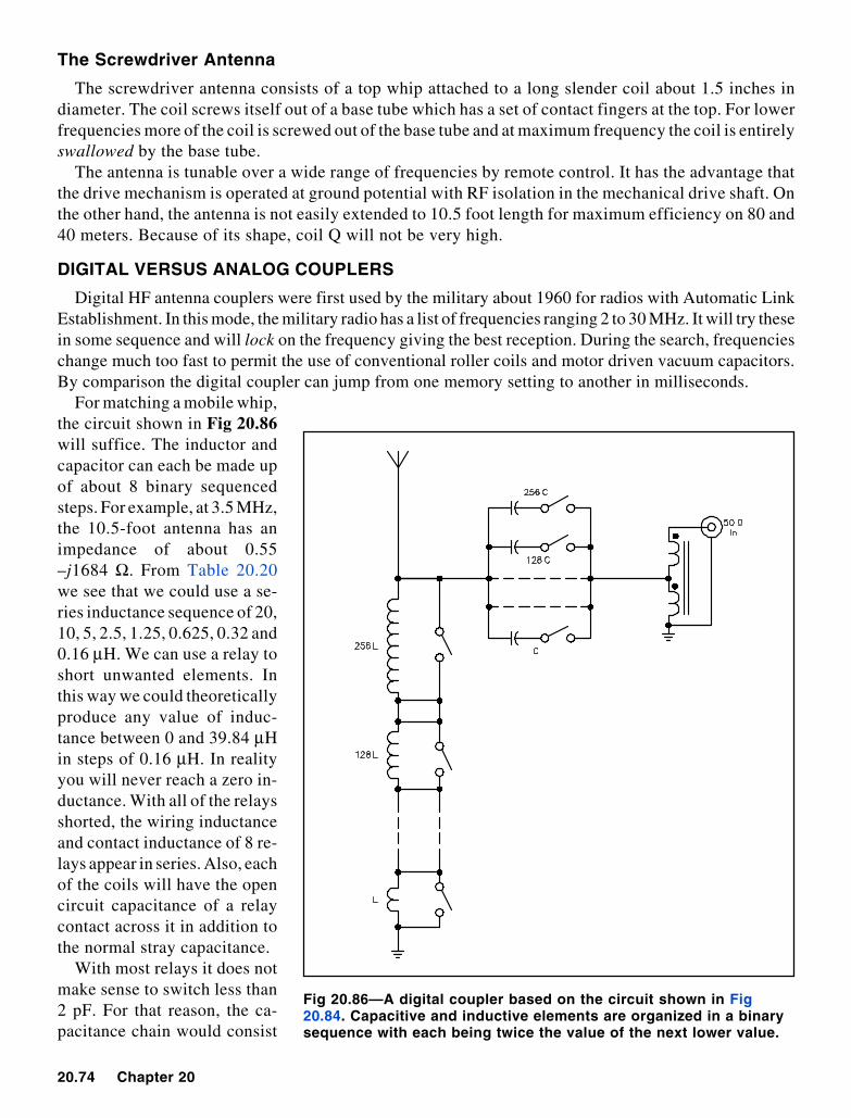
20.74 Chapter 20
The Screwdriver Antenna
The screwdriver antenna consists of a top whip attached to a long slender coil about 1.5 inches indiameter. The coil screws itself out of a base tube which has a set of contact fingers at the top. For lowerfrequencies more of the coil is screwed out of the base tube and at maximum frequency the coil is entirelyswallowed by the base tube.
The antenna is tunable over a wide range of frequencies by remote control. It has the advantage thatthe drive mechanism is operated at ground potential with RF isolation in the mechanical drive shaft. Onthe other hand, the antenna is not easily extended to 10.5 foot length for maximum efficiency on 80 and40 meters. Because of its shape, coil Q will not be very high.
DIGITAL VERSUS ANALOG COUPLERS
Digital HF antenna couplers were first used by the military about 1960 for radios with Automatic LinkEstablishment. In this mode, the military radio has a list of frequencies ranging 2 to 30 MHz. It will try thesein some sequence and will lock on the frequency giving the best reception. During the search, frequencieschange much too fast to permit the use of conventional roller coils and motor driven vacuum capacitors.By comparison the digital coupler can jump from one memory setting to another in milliseconds.
For matching a mobile whip,the circuit shown in Fig 20.86will suffice. The inductor andcapacitor can each be made upof about 8 binary sequencedsteps. For example, at 3.5 MHz,the 10.5-foot antenna has animpedance of about 0.55–j1684 Ω. From Table 20.20we see that we could use a se-ries inductance sequence of 20,10, 5, 2.5, 1.25, 0.625, 0.32 and0.16 µH. We can use a relay toshort unwanted elements. Inthis way we could theoreticallyproduce any value of induc-tance between 0 and 39.84 µHin steps of 0.16 µH. In realityyou will never reach a zero in-ductance. With all of the relaysshorted, the wiring inductanceand contact inductance of 8 re-lays appear in series. Also, eachof the coils will have the opencircuit capacitance of a relaycontact across it in addition tothe normal stray capacitance.
With most relays it does notmake sense to switch less than2 pF. For that reason, the ca-pacitance chain would consist
Fig 20.86—A digital coupler based on the circuit shown in Fig20.84. Capacitive and inductive elements are organized in a binarysequence with each being twice the value of the next lower value.

Antennas & Projects 20.75
of 2, 4, 8, 16, 32, 64, 128 and possibly 256 pF. This would give a maximum of 510 pF and a step sizeof 2 pF. Each relay has an open circuit capacitance of about 1 pF, and that gives a minimum capacitanceof 8 to 9 pF. As a practical matter, there is also the stray capacitance between the relay contacts and thecoil windings.
In a high Q matching circuit that handles 100 W, the individual relays must handle 4 or 5 kV withthe contacts open and several amperes of RF with the contacts closed. If we can unkey the transmitterso that the coupler will not have to switch under power, we’ll still need some sizeable relays. If theinductors have lower Q, the voltages and currents will be correspondingly lower. Some militarycouplers use Jennings vacuum latching relays. This is expensive, as each of the 16 or 17 relays costsmore than $100.
If coil and antenna Qs are kept or forced low, the voltages and currents become more reasonable.However, if the antenna size is restricted this reduction comes only at the cost of decreased efficiency.A commercially available ham/marine digital coupler employs RF reed relays rated for 5 kV and 1 A,and restricts the power at low frequencies if the antenna is small. Another ham/marine unit uses smallrelays in series where voltage requirements are great and in parallel where current requirements aregreat—not good engineering practice. A third offering is not too specific about the power rating withvery high Q loads.
There are no successful examples of 100 W plus couplers that use PIN diode switching. Their use ishighly problematic given the high-Q loads they would handle.
A REMOTELY TUNED ANALOG ANTENNA COUPLER
KE2QJ built an antenna coupler designed for 100-W continuous-duty operation that will tune anantenna 10 feet or longer to any frequency from 3.5 to 30 MHz. With longer antennas, the power ratingis higher and the lowest frequency is lower. The design requires only hand tools to build; however, accessto a drill press and a lathe could save labor.
The roller coils and air variable capacitors to be used are not widely manufactured these days. Tube-type linear amplifiers still use air variable capacitors but these are generally built on order for themanufacturer and are not readily available to consumers in small quantity.
Until the 1970s, E. F. Johnson manufactured roller coils and air variable capacitors that were suitablefor kilowatt amplifier finals and high power antenna couplers. On occasion one or more of these maybe found in the original box, but they tend to be expensive. Ten Tec and MFJ both manufacture antennacouplers and offer some components in small quantities.
The following data refer to generic motors, capacitors and inductors. The descriptions are intendedto aid the builder in selecting items from surplus, hamfest flea market offerings or salvage of oldequipment.
THE MOTORS
Two motors are required, one to drive the inductor and one to drive the capacitor. The design employspermanent magnet dc gearhead motors with a nominal 12-V rating. A permanent magnet (PM) motorcan be reversed by simply reversing the polarity of the drive voltage, and its speed can be controlled overa wide range by pulsing the power on and off with a variable duty cycle. The motor should have an outputshaft speed on the order of 60 to 180 r/min (1 to 3 r/s) although this is not critical. New, such motors,can cost as much as $65 to $150 in small quantities. However, they can be found surplus and in repairshops for a few dollars.
The motor you are looking for is 1 to 1.5 inches in diameter and perhaps 2.5 inches long. It might berated 12 or 24 V and have a 1/4-inch diameter output shaft. At 12 V it should have enough torque to makeit hard to stop the shaft with your fingers. Tape recorders, fax machines, film projectors, windshieldwipers and copiers often use this type of motor.

20.76 Chapter 20
LIMIT SWITCHES
On a remotely operated unit it is usually necessary to have limit switches to prevent the device fromcrashing into the ends. On an external roller coil these can be microswitches with paddles mounted oneach end of the coil. As the coil is wound to one end, the roller operates the paddle and opens the limitswitch which stops the motor.
Fig 20.87A illustrates a simple motor control circuit. Relay K1 is arranged as a DPDT polarityreversing switch. If switch CCW is pressed, the motor rotates CCW and the steering diode prevents therelay from operating. If CW is pressed, relay K1 operates reversing the polarity at the motor. The motoris energized through the steering diode.
Fig 20.87B shows how to add limit switches.The diodes across the switches are called anti-jamdiodes. When a switch opens, the diode permitscurrent to flow in the reverse direction and themotor to move the roller away from the openswitch.
The photograph of Fig 20.88 shows themounting of the switches on the coil. The diodeshould be a power rectifier type rated for severaltimes the motor current and at least 60 V.
POSITION READER
While not necessary, it is worthwhile to have away to determine inductor position. An easy way
Fig 20.87—At A, motor control circuit used by KE2QJ. This circuit uses pulse modulation for speedcontrol with good starting torque. Direction of rotation is controlled by the relay. At B, how to addlimit switches to the circuit. See text.
Fig 20.88—Photo of the inductor drive assemblyfrom KE2QJ’s antenna coupler.

Antennas & Projects 20.77
to do this is to couple a 10-turn potentiometer to the coil shaft or drive gears. Make sure that thepotentiometer turns less than 10 turns between limits. Don’t try to make it come out exact.
Because the potentiometer is a light mechanical load, a belt drive reduction works well and won’t slipif properly tensioned. Fig 20.87A shows the potentiometer and the gear drive.
You may be able to find suitable gears. However, a belt drive requires less precise shaft positioningthan fine tooth gears. With a lathe, pulleys can be made in almost any ratio. Vacuum cleaner belts andO rings make handy belts.
COUPLINGS
In this coupler circuit, both ends of the capacitor are hot with RF although the end adjacent to thetransformer is at relatively low voltage. Nevertheless, the capacitor shaft must be insulated from themotor shaft. The coil can be driven from the grounded end. Insulation is not necessary, but use a couplerbetween the motor shaft and the coil to compensate for any misalignment. Universal joints and insulatingcouplings are available from most electronics supply houses. You can make a coupling from a length offlexible plastic tubing which fits snugly over the shafts. Clamp the tubing to the shafts to avoid slippage.
THE CAPACITOR
The easiest capacitor to use is an air variable. It should have a range of approximately 10 to 250 pF.The plate spacing should be 2 mm (1/16 inch) or more, and the plate edges should be smooth and rounded.The capacitor should be capable of continuous 360° rotation, and it would be nice if it had ball bearings.The straight-line capacitance design is best for this application. Several capacitors of this type areavailable in military surplus ARC-5 series transmitters. These are approximately 2 × 2 × 3 inches.
The capacitor must be mounted on stand-off insulators although high voltage will not be present onthe frame. A cam that briefly operates a microswitch when the capacitor goes through minimum can beused to flash an LED on the remote control panel. This provides an indication that the capacitor isturning.
THE INDUCTOR
As calculated earlier, and assuming an inductor Q a bit under 300 is attainable, the roller inductor forthis coupler should have a maximum inductance on the order of 40 µH. The wire should be at least#14 AWG wound about 8 t/inch.
You can use Table 20.21 as a guide to buy a roller coil at a hamfest. The seller may not know theinductance of the coil. The antenna loading coil from an ARC-5 transmitter will work, but the wire isa bit small.
You could make the loading coil by threading 2, 2.5 or 3-inch diameter white, thick-wall PVC pipewith 8 t/inch. If the pipe is threaded in a lathe, the wire can be wound into the threads under considerabletension. This helps to prevent the wires from coming loose with wear or temperature.
THE TRANSFORMER
The transformer consists of a bifilar winding on an Amidon FT-114-61 core. Start with two 2-foot lengths of #18 insulated wire;Teflon insulation is preferable. Twist the wire with a hand drill untilthere are about 5 t/inch (not critical). Wind 12 turns onto the core.This should about fill it up. Attach the starting end of one wire to thefinish end of the other. This is the 12.5-Ω tap. One of the free ends isgrounded and the other is the 50-Ω tap. Mount the coil on a plastic orwooden post through the center of the coil. A metal screw can be usedas long as it does not make a complete turn around the core.
Table 20.21Data for 40 µµµµµH Coils
Diameter Length Turns2.3 inch 5.625 inch 45(58 mm) (143 mm)2.8 inch 4.25 inch 34(71 mm) (108 mm)3.3 inch 3.375 inch 27(84 mm) (86 mm)

20.78 Chapter 20
CONSTRUCTION
For ease of service, mount the inductor, its drive motor, position sensing potentiometer and limitswitch assembly on a single aluminum plate. A plug and socket assembly permits rapid disconnectionand removal. Make a similar assembly for the capacitor, its drive motor, transformer and the interrupter.Both assemblies should be made on 1/16 to 1/8-inch thick aluminum. These individual assemblies makeit easier to fix problems.
The chassis shown in Fig 20.89A is made of a single piece 1/16 to 3/32-inch aluminum bent in an Lshape. Two chassis-stiffening braces are riveted in place. Alternatively, the chassis can be made of flatsheets with aluminum angles riveted around the edge.
Mount the coil and capacitor assemblies parallel to the long leg of the L. Punch a 1-inch hole in the centerof the short end of the L. Cover the hole with an insulator made of PVC, Teflon or other suitable material.
The rest of the case is a 4-sided wooden assembly as shown in Fig 20.89B. The back wall of the boxis drilled to accept the two pivot pins. The box is slid over the chassis and the pivot pins engaged. Thetie-down screw secures the box. For service, remove the tie-down screw and slide off the cover. Theworks of the coupler are veryeasy to get at!
The box is made of 1/4-inchexterior grade plywood exceptfor the back plate, which is 3/8
or 1/2-inch plywood. The sides,top and back should overlap theflanges on the chassis by 1/2
inch. The inside corner seamsof the box should be reinforcedwith 1/2 or 3/4-inch squarestrips. Assembly can be withany water resistant glue.
Finish the box, inside andout, with several coats of clearurethane varnish, sandinglightly between coats. Thisleaves a smooth plastic finish.This can be sprayed with anexterior paint that matchesyour car’s color.
If the sides of the box fitclosely over the flanges, nofastening beside the tie-downscrew is required. A nearlyperfect seal will leak out hot airwhen the sun shines on it andwill draw in cold damp air inthe evening, trapping moistureinside. A moderate fit will keeprain and snow out and permitthe box to breathe freely,thereby keeping the inside dry.
Fig 20.89—At A, the chassis for the coupler mounting box. At B,the box cover.

Antennas & Projects 20.79
MOUNTING THE WHIP AND THE BOXPlastics in bumpers and bodies makes the mounting of a mobile whip antenna problematic. Modern
bumpers are covered with plastic and the bumper is attached to the car unibody through a 5-MPH shockabsorber. The latter item is an unreliable ground.
The arrangement of Fig 20.90 solves many of these problems. It uses a 1/4-inch aluminum plate 6 to8 inches wide and long enough to fit between a reasonably strong place on the unibody and the placebehind the bumper where the antenna wants to be. This plate is fitted with an angle bracket for the lowerbolt on the shock/bumper mounting. This plate is stiffened with a length of 1 × 1 × 1/4-inch aluminumangle bolted in several places.
Near the forward edge of the plate, two 1/2-inch diameter aluminum shear posts are fitted. Thebottom of each is tapped 10-32 and bolted through the mount plate with a stainless 10-32 screw. Atthe top of these shear posts another piece of 1 × 1 × 1/2-inch angle is attached which is screwed to theunibody with three or four #10 stainless sheet metal screws. A bracket attaches the mount plate to thebumper’s shock absorber. The angle bracket may either be welded to the plate or bolted with anglestock. In the event that the car is hit from behind or backs into an obstacle, the two 10-32 screws willshear off, thereby preventing the mount fromdefeating the 5 MPH crushable shock absorber.The part protruding behind the bumper may becut down in width to 3 inches and rounded forappearance and safety.
Any type of base insulator may be used, buttry to bring the base of the antenna to the heightof the coupler output terminal. You can make agood base insulator from thick-wall white PVC11/2 inch pipe. Reinforce each end. Start with a11/2 inch length of pipe. Remove a 5/8-inch widestrip so the remaining portion can be rolled andpressed into the open end of the insulator. ApplyPVC pipe glue just before pressing in the piece;this gives the insulator a double wall thickness ateach end. Aluminum plugs can be turned for asnug fit and tapped for 3/8-24 hardware. Theplugs can be held in place with 8-32 stainlessscrews.
The upper antenna brace has an aluminumplate at one end that goes under the trunk lid (seeFig 20.90). A length of 1/2-inch diameter heavy-wall white PVC pipe, which serves as an insula-tor, is screwed to this. At the other end of theinsulator, another aluminum piece is bent to forma saddle for the antenna which is clamped to thesaddle. This clamp should be as high as conve-nient above the mount plate, preferably not lessthan a foot. The mount plate should be sturdyenough for you to stand on and with the bracewill easily hold a whip upright at 70 MPH ormore.
Fig 20.90—Antenna mounting detail. At A, theoverall plan. At B, detail of the mount plate.

20.80 Chapter 20
The coupler box mounting is shown in Fig 20.91. Brackets canbe made of 1/8 × 2-inch aluminum with a brace going perhaps 2inches from the corner. The brackets bolt or rivet to the chassis.The bracket reaches through the gap between the trunk lid and theplastic top of the bumper. For reinforcement, a pair of reinforce-ment plates 1.5 × 2 × 1/4-inch thick are bolted to the plastic on theunder side of the bumper. Ground the rein-forcement plates to theunibody with some 3/4 or 1 inch ground braid.
Two 10-32 stainless screws hold each reinforcement plate to theplastic bumper and a central 1/4-20 tapped hole holds down thebox bracket. One need only remove two screws to get the box offthe car for car wash, etc. You have to open the trunk to remove theantenna coupler, and this provides a measure of security.
THE SPRING AND WHIP
A section of 1-inch diameter aluminum tubing extends from thetop of the insulator to the base of the spring. It’s usually best tohave the spring about 4 feet above the pavement. The type used forCB whips works well. A 7-foot whip brings the top to about 11.5feet above the pavement. The 7-foot whip can be a cut down CBunit. Don’t use the type with helical winding. When the antennais tied down, the bow of the whip should be about 7 feet above thepavement.
TUNING
It is best to initially tune the antenna using low power. A powerattenuator just after the transceiver will limit SWR, but your SWRindicator must be on the antenna side of the attenuator.
For a first tune-up set the capacitor control to SCAN and slowlyadvance the inductor from minimum inductance toward maxi-mum. As the inductor approaches the correct value the SWR willstart to kick down. At this point take the capacitor off of SCAN and JOG it to a best tune. Next, JOG theinductor and repeat; the SWR should go down. Continue until a 1:1 SWR is obtained. Record thepotentiometer setting. The next time you want to use this frequency run the coil directly to the loggedsetting.
In the SCAN position the capacitor motor runs at full voltage. When you JOG the capacitor for low SWRyou will find the speed far too fast for sharp tuning. The slow speed tuning is provided by using duty-factor modulation of the motor current. The circuit of Fig 20.87A supplies fixed width pulses withvariable timing. At the slowest speed, the unit will supply about one pulse per second and the motor shaftwill rotate one degree or so per pulse. The full voltage pulse provides good starting torque.
If the SWR cannot be brought to 1:1, examine the coil and capacitor to see whether either is atmaximum or minimum. At high frequencies above 24 MHz it may be necessary to place a capacitorbetween the coupler and the antenna base.
RADIATION PATTERNS
At the lower frequencies the pattern tends to be essentially round in azimuth. At 20 meters the patterntends to become more and more directive. The patterns in Fig 20.92 were calculated using EZNEC. Thefrequency is 18.13 MHz and the antenna is mounted at the left rear corner of a mid-size sedan. It may
Fig 20.91—Box mounting detail.At A, mounting-bracket design.At B, photo of KE2QJ’s installa-tion.
(B)

Antennas & Projects 20.81
be seen that the pattern has more than 10 dB maximum-to-minimum ratio with the broad maximum along the diagonal of thevehicle occupied by the antenna. If the antenna were mounted inthe center of the vehicle, the omnidirectional characteristics wouldbe improved. However, the antenna would have to be much shorterto stay under 11.5 feet. The shorter antenna would likely be weakerin its best direction than the taller antenna is in its worst.
References
J. S. Belrose, VE3BLW, “Short Antennas for Mobile Operation,”QST, Sept 1953, pp 30-35, 109.
J. Kuecken, KE2QJ, Antennas and Transmission Lines, MFJPublishing, Ch 25.
J. Kuecken, KE2QJ, “A High Efficiency Mobile Antenna Cou-pler,” The ARRL Antenna Compendium, Vol 5, pp 182-188.
J. Kuecken, KE2QJ, “Easy Homebrew Remote Controls,” TheARRL Antenna Compendium, Vol 5, pp 189-193.
J. Kuecken, KE2QJ, “A Remote Tunable Center Loaded An-tenna,” The ARRL Antenna Compendium, Vol 6.
Fig 20.92—At A, elevation patternof the KE2QJ mobile antenna.The pattern is in the plane thatruns diagonal through the car. AtB, azimuth pattern at 25° eleva-tion for the same antenna. Theoperating frequency is 18.130MHz.

20.82 Chapter 20
VHF/UHF AntennasINTRODUCTION
Improving an antenna system is one of the most productive moves open to the VHF enthusiast. It canincrease transmitting range, improve reception, reduce interference problems and bring other practicalbenefits. The work itself is by no means the least attractive part of the job. Even with high-gain antennas,experimentation is greatly simplified at VHF and UHF because an array is a workable size, and much canbe learned about the nature and adjustment of antennas. No large investment in test equipment is necessary.
Whether we buy or build our antennas,we soon find that there is no one “best” design for all purposes.Selecting the antenna best suited to our needs involves much more than scanning gain figures and pricesin a manufacturer’s catalog. The first step should be to establish priorities.
Gain
As has been discussed previously, shaping the pattern of an antenna to concentrate radiated energy,or received signal pickup, in some directions at the expense of others is the only possible way to developgain. Radiation patterns can be controlled in various ways. One is to use two or more driven elements,fed in phase. Such arrays provide gain without markedly sharpening the frequency response, comparedto that of a single element. More gain per element, but with some sacrifice in frequency coverage, isobtained by placing parasitic elements into a Yagi array.
Radiation Pattern
Antenna radiation can be made omnidirectional, bidirectional, practically unidirectional, or anythingbetween these conditions. A VHF net operator may find an omnidirectional system almost a necessitybut it may be a poor choice otherwise. Noise pickup and other interference problems tend to be greaterwith omnidirectional antennas. Maximum gain and low radiation angle are usually prime interests of theweak-signal DX aspirant. A clean pattern, with lowest possible pickup and radiation off the sides andback, may be important in high-activity areas, where the noise level is high, or when challenging modeslike EME (Earth-Moon-Earth) are employed.
Height Gain
In general, the higher a VHF antenna is installed, the better will be the results. If raising the antenna clearsits view over nearby obstructions, it may make dramatic improvements in coverage. Within reason, greaterheight is almost always worth its cost, but height gain must be balanced against increased transmission-lineloss. Line losses can be considerable at VHF, and they increase with frequency. The best available line maybe none too good, if the run is long in terms of wavelength. Consider line losses in any antenna planning.
Physical Size
A given antenna design for 432 MHz, say a 5-element Yagi on a 1-λ boom, will have the same gainas one for 144 MHz, but being only one-third the size it will intercept only one-ninth as much energyin receiving. Thus, to be equal in communication effectiveness, the 432-MHz array should be at leastequal in physical size to the 144-MHz one, requiring roughly three times the number of elements. Withall the extra difficulties involved in going higher in frequency, it is well to be on the big side in buildingan antenna for the UHF bands.
DESIGN FACTORS
Having sorted out objectives in a general way, we face decisions on specifics, such as polarization,type of transmission line, matching methods and mechanical design.

Antennas & Projects 20.83
Polarization
Whether to position the antenna elements vertically or horizontally has been a question since earlyVHF pioneering. Tests show little evidence on which to set up a uniform polarization policy. On longpaths there is no consistent advantage, either way. Shorter paths tend to yield higher signal levels withhorizontal in some kinds of terrain. Man-made noise, especially ignition interference, tends to be lowerwith horizontal. Verticals, however, are markedly simpler to use in omnidirectional systems and inmobile work.
Early VHF communication was largely vertical, but horizontal gained favor when directional arraysbecame widely used. The major trend to FM and repeaters, particularly in the 144-MHz band, has tippedthe balance in favor of verticals in mobile work and for repeaters. Horizontal predominates in othercommunication on 50 MHz and higher frequencies. It is well to check in advance in any new area inwhich you expect to operate, however, as some localities may use vertical polarization. A circuit lossof 20 dB or more can be expected with cross-polarization.
Transmission Lines
There are two main categories of transmission lines used at HF through UHF: balanced and unbal-anced. Balanced lines include open-wire lines separated by insulating spreaders, and twin-lead, in whichthe wires are embedded in solid or foamed insulation. Unbalanced lines are represented by the familyof coaxial cables, commonly called coax. Line losses in either types of line result from ohmic resistance,radiation from the line and deficiencies in the insulation.
Large conductors, closely spaced in terms of wavelength, and using a minimum of insulation, makethe best balanced lines. Characteristic impedances are between 300 to 500 Ω. Balanced lines work bestin straight runs, but if bends are unavoidable, the angles should be as gentle as possible. Care should alsobe taken to prevent one wire from coming closer to metal objects than the other.
Properly built open-wire line can operate with very low loss in VHF and even UHF installations. Atotal line loss under 2 dB per hundred ft at 432 MHz is readily obtained. A line made of #12 wire, spaced3/4 inch or less with Teflon spreaders, and running essentially straight from antenna to station, can bebetter than anything but the most expensive “Hardline” coax, at a fraction of the cost. This assumes theuse of high-quality baluns to match into and out of the balanced line, with a short length of low-loss coaxfor the rotating section from the top of the tower to the antenna. A similar 144-MHz setup could havea line loss under 1 dB.
Small coax such as RG-58 or RG-59 should never be used in VHF work if the run is more than a fewfeet. Half-inch lines (RG-8 or RG-11) work fairly well at 50 MHz, and are acceptable for 144-MHz runsof 50 ft or less. If these lines have foam rather than solid insulation they are about 30% better. Aluminum-jacket “Hardline” coaxial cables with large inner conductors and foam insulation are well worth theircost. Hardline can sometimes even be obtained for free from local Cable TV operators as “endruns”æpieces at the end of a roll. The most common CATV variety is 1/2-inch OD 75-Ω Hardline.Waterproof commercial connectors for Hardline are fairly expensive, but enterprising amateurs have“home-brewed” low-cost connectors. If they are properly waterproofed, connectors and Hardline canlast almost indefinitely. Of course, a disadvantage implied by their name is that Hardline must not bebent too sharply, because it will kink. See The ARRL Antenna Book for details on Hardline connectors.
Effects of weather on transmission lines should not be ignored. A well-constructed open-wire lineworks well in nearly any weather, and it stands up well. TV type twin-lead is almost useless in heavyrain, wet snow or icing. The best grades of coax are impervious to weather. They can be run underground,fastened to metal towers without insulation, or bent into almost any convenient position, with no adverseeffects on performance. However, beware of “bargain” coax. Lost transmitter power can be made up tosome extent by increasing power, but once lost, a weak signal can never be recovered in the receiver.

20.84 Chapter 20
Impedance Matching
Theory and practice in impedance matching are given in detail in the Transmission Lines chapter,and in theory, at least, is the same for frequencies above 50 MHz. Practice may be similar, but physicalsize can be a major modifying factor in choice of methods.
Delta Match
Probably the first impedance match was made when the ends of an open line were fanned out andtapped onto a half-wave antenna at the point of most efficient power transfer, as in Fig 20.93A. Boththe side length and the points of connection either side of the center of the element must be adjusted forminimum reflected power in the line, but the impedances need not be known. The delta makes noprovision for tuning out reactance, so the length of the dipole is pruned for best SWR.
Once thought to be inferior for VHF applications because of its tendency to radiate if adjustedimproperly, the delta has come back to favor now that we have good methods for measuring the effectsof matching. It is very handy for phasing multiple-bay arrays with low-loss open lines, and its dimensionsin this use are not particularly critical.
Gamma and T Matches
The gamma match is shown in Fig 20.93C,and the T match is shown in Fig 20.93D. Thesematches are covered in more detail in the chapteron Transmission Lines. There being no RFvoltage at the center of a half-wave dipole, theouter conductor of the coax is connected to theelement at this point, which may also be the junc-tion with a metallic or wooden boom. The innerconductor, carrying the RF current, is tapped outon the element at the matching point. Inductanceof the arm is canceled by means of C1. Both thepoint of contact with the element and the settingof the capacitor are adjusted for zero reflectedpower, with a bridge connected in the coaxialline.
The capacitor can be made variable tempo-rarily, then replaced with a suitable fixed unitwhen the required capacitance value is found, orC1 can be mounted in a waterproof box. Maxi-mum capacitance should be about 100 pF for50 MHz and 35 to 50 pF for 144 MHz. The ca-pacitor and arm can be combined with the armconnecting to the driven element by means of asliding clamp, and the inner end of the arm slid-ing inside a sleeve connected to the inner con-ductor of the coax. It can be constructed fromconcentric pieces of tubing, insulated by plasticsleeving or shrink tubing. RF voltage across thecapacitor is low, once the match is adjusted prop-erly, so with a good dielectric, insulation pre-
Fig 20.93—Matching methods commonly used inVHF antennas. In the delta match, A and B, theline is fanned out to tap on the dipole at the pointof best impedance match. The gamma match, C, isfor direct connection of coax. C1 tunes out induc-tance in the arm. Folded dipole of uniformconductor size, D, steps up antenna impedance bya factor of four. Using a larger conductor in theunbroken portion of the folded dipole, E, giveshigher orders of impedance transformation.
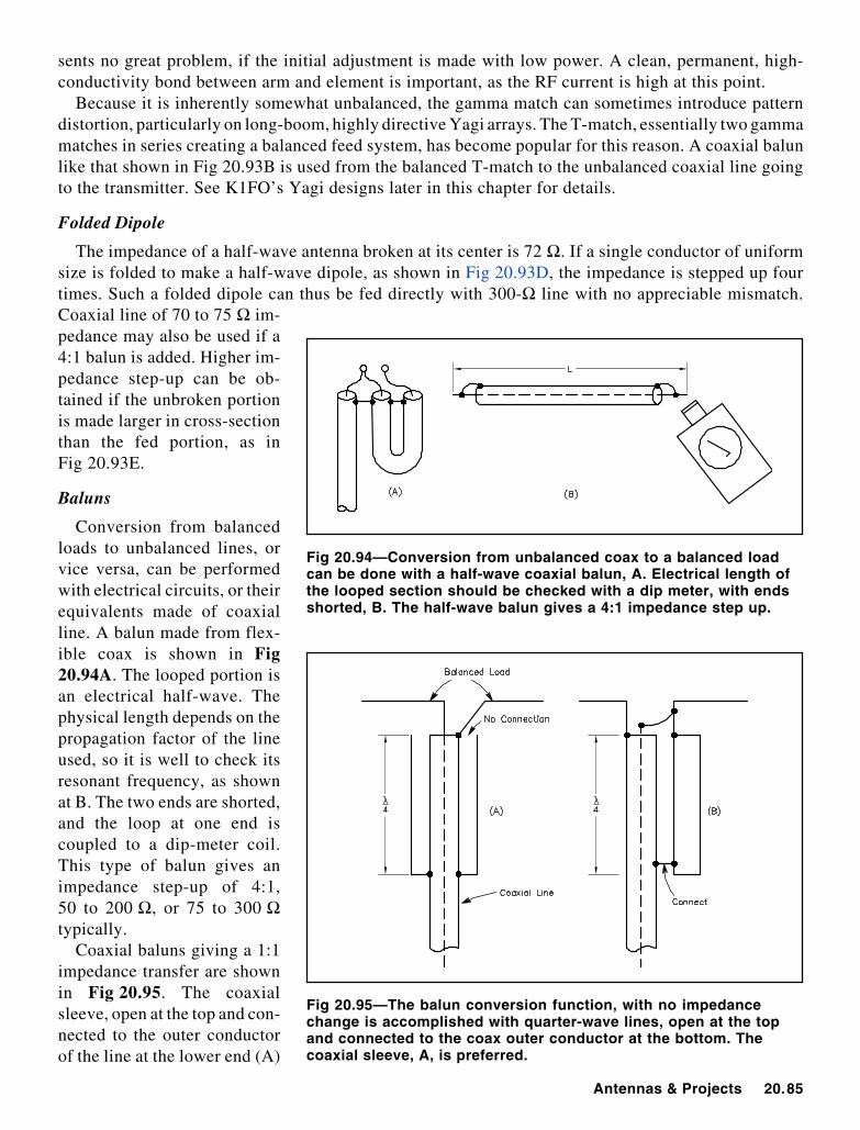
Antennas & Projects 20.85
sents no great problem, if the initial adjustment is made with low power. A clean, permanent, high-conductivity bond between arm and element is important, as the RF current is high at this point.
Because it is inherently somewhat unbalanced, the gamma match can sometimes introduce patterndistortion, particularly on long-boom, highly directive Yagi arrays. The T-match, essentially two gammamatches in series creating a balanced feed system, has become popular for this reason. A coaxial balunlike that shown in Fig 20.93B is used from the balanced T-match to the unbalanced coaxial line goingto the transmitter. See K1FO’s Yagi designs later in this chapter for details.
Folded Dipole
The impedance of a half-wave antenna broken at its center is 72 Ω. If a single conductor of uniformsize is folded to make a half-wave dipole, as shown in Fig 20.93D, the impedance is stepped up fourtimes. Such a folded dipole can thus be fed directly with 300-Ω line with no appreciable mismatch.Coaxial line of 70 to 75 Ω im-pedance may also be used if a4:1 balun is added. Higher im-pedance step-up can be ob-tained if the unbroken portionis made larger in cross-sectionthan the fed portion, as inFig 20.93E.
Baluns
Conversion from balancedloads to unbalanced lines, orvice versa, can be performedwith electrical circuits, or theirequivalents made of coaxialline. A balun made from flex-ible coax is shown in Fig20.94A. The looped portion isan electrical half-wave. Thephysical length depends on thepropagation factor of the lineused, so it is well to check itsresonant frequency, as shownat B. The two ends are shorted,and the loop at one end iscoupled to a dip-meter coil.This type of balun gives animpedance step-up of 4:1,50 to 200 Ω, or 75 to 300 Ωtypically.
Coaxial baluns giving a 1:1impedance transfer are shownin Fig 20.95. The coaxialsleeve, open at the top and con-nected to the outer conductorof the line at the lower end (A)
Fig 20.94—Conversion from unbalanced coax to a balanced loadcan be done with a half-wave coaxial balun, A. Electrical length ofthe looped section should be checked with a dip meter, with endsshorted, B. The half-wave balun gives a 4:1 impedance step up.
Fig 20.95—The balun conversion function, with no impedancechange is accomplished with quarter-wave lines, open at the topand connected to the coax outer conductor at the bottom. Thecoaxial sleeve, A, is preferred.

20.86 Chapter 20
is the preferred type. A conductor of approximately the same size as the line is used with the outerconductor to form a quarter-wave stub, in B. Another piece of coax, using only the outer conductor, willserve this purpose. Both baluns are intended to present an infinite impedance to any RF current that mightotherwise tend to flow on the outer conductor of the coax.
Stacking Yagis
Where suitable provision can be made for supporting them, two Yagis mounted one above the otherand fed in phase may be preferable to one long Yagi having the same theoretical or measured gain. Thepair will require a much smaller turning space for the same gain, and their lower radiation angle canprovide interesting results. On long ionospheric paths a stacked pair occasionally may show an apparentgain much greater than the 2 to 3 dB that can be measured locally as the gain from stacking.
Optimum spacing for Yagis with booms longer than 1 λ is one wavelength, but this may be too muchfor many builders of 50-MHz antennas to handle. Worthwhile results are possible with as little as 1/2 λ(10 ft), but 5/8 λ (12 ft) is markedly better. The difference between 12 and 20 ft may not be worth theadded structural problems involved in the wider spacing, at 50 MHz at least.
The closer spacings give lowered measured gain, but the antenna patterns are cleaner (less power in thehigh-angle elevation lobes) than with one-wavelength spacing. Extra gain with wider spacings is usually theobjective on 144 MHz and higher bands, where the structural problems are not quite as severe as on 50 MHz.
One method for feeding two 50-Ω antennas, as might be used ina stacked Yagi array, is shown in Fig 20.96. The transmissionlines from each antenna, with a balun feeding each antenna (notshown in the drawing for simplicity), to the common feedpointmust be equal in length and an odd multiple of a quarter wave-length. This line acts as an quarter-wave (Q-section) impedancetransformer and raises the feed impedance of each antenna to100 Ω. When the coaxes are connected in parallel at the coaxial Tfitting, the resulting impedance is close to 50 Ω.
Circular Polarization
Polarization is described as “horizontal” or “vertical,” but theseterms have no meaning once the reference of the Earth’s surface islost. Many propagation factors can cause polarization change—reflection or refraction and passage through magnetic fields (Faradayrotation), for example. Polarization of VHF waves is often random,so an antenna capable of accepting any polarization is useful. Circularpolarization, generated with helical antennas or with crossed ele-ments fed 90° out of phase, will respond to any linear polarization.
The circularly polarized wave in effect threads its way throughspace, and it can be left- or right-hand polarized. These polariza-tion senses are mutually exclusive, but either will respond to anyplane (horizontal or vertical) polarization. A wave generated withright-hand polarization, when reflected from the moon, comesback with left-hand plarization, a fact to be borne in mind insetting up EME circuits. Stations communicating on direct pathsshould have the same polarization sense.
Both senses can be generated with crossed dipoles, with the aidof a switchable phasing harness. With helical arrays, both sensesare provided with two antennas wound in opposite directions.
Fig 20.96—A method for feedinga stacked Yagi array. Note thatbaluns at each antenna are notspecifically shown. Modern-daypractice is to use current(“choke”) baluns made up offerrite beads slipped over theoutside of the coax and taped toprevent movement. See Trans-mission Lines chapter for details.

Antennas & Projects 20.87
/"#=#= "%
There is a very simple and inexpensive way to strengthen your beam antenna prior to hoisting it tothe top of the tower. Most well-stocked hardware stores stock assorted sizes of hardwood dowel.Select dowels that can be snugly inserted inside the boom and elements and placed where they areattached to each other. Carefully redrill any holes blocked by the dowels and assemble the beam asinstructed. You will then have a more solid attachment point and can really tighten the U-bolts andfittings without fear of deforming the tubing. Lightweight beams can be strengthened by inserting thedowel in the entire length of the boom. This method can be used to straighten elements that havebeen damaged. These dowels add very little weight to the antenna. I have done this for over 25 yearsand am completely satisfied with the results.—H. A. “Tony” Miller, W5BWA, Alexandria, Louisiana
" /"@&"$1" =
My antenna rotator manual says that the rotator’s lubricant should flow at temperatures below–20 °F, but during a –28° spell last winter, nothing moved. I attached a magnetically mounted carengine heater to the bottom of the rotator mounting plate, warmed up the rotator, and got it movingagain. —Richard Mollentine, WA0KKC, Overland Park, Kansas
>17 "66/A
Here is a functional antenna for 223 MHz that you can make inless than an hour (Fig A). To build it, you’ll need 9 feet of #10copper wire, 6 inches of small-diameter copper tubing, and a10-foot length of PVC pipe or some other physical support.
Bend the antenna from one piece of wire. Slide the coppertubing over the top end of the antenna, and adjust how far itextends beyond the wire to get the lowest SWR. (Don’t handle theantenna while transmitting—make adjustments only while receiv-ing.) For more precision, you can move the coaxial feed line’staps on the antenna’s matching stub (the 12-inch section at thebottom) about an eighth of an inch at a time. My antenna showsan SWR of 1.2 at 223 MHz.—William Bruce Cameron, WA4UZM,Temple Terrace, Florida
Fig A—WA4UZM’s quick 223-MHz antenna gets you goingon 11/4 meters in a hurry. (Thetext explains how to adjust itfor minimum SWR.) To supportthe antenna, lash it to a pieceof PVC pipe with nylon cableties.

20.88 Chapter 20
5(λλλλλ!/!* !Quarter-wave vertical antennas are useful for local communications when size, cost and ease of
construction are important. For theoretical information about quarter-wave vertical antennas see earlierparts of this chapter or The ARRL Antenna Book.
Construction Materials
The antennas shown in the following sections are built on a coaxial connector. Use UHF or N con-nectors for the fixed station antennas. BNC connectors are good for mobile and portable antennas. BNCand N connectors are better than PL-259 connectors for VHF/UHF outdoor use because: (1) they providea constant impedance over the frequencies of interest, and (2) they are weatherproof when the appro-priate connector or cap is attached. The ground-plane antennas require a panel-mount connector (it hasmounting holes to hold the radials).
If the antenna is sheltered from weather, copper wire is sufficiently rigid for the element and radials.Antennas exposed to the weather should be made from 1/16- to 1/8-inch brass or stainless-steel rod.
Radials may be made from3/16-inch aluminum rod or tub-ing and mounted on an alumi-num sheet. Do not use alumi-num for the antenna elementbecause it cannot be easily sol-dered to the coaxial-connectorcenter pin.
Where the figures call for#4-40 hardware, stainless steelor brass is best. Use cadmium-plated hardware if stainlesssteel or brass is not available.
Fixed-Station Antennas
The ground-plane antenna inFig 20.97 uses female chassis-mount connectors to supportthe element and four radials. Ifyou have chosen large-diam-eter wire or tubing for the radi-als refer to Fig 20.98. Cut ametal sheet as shown (size isnot critical, and the mountingtab is optional). Drill the sheetto accept the coaxial connectoron hand (usually 11/16 inch) andthe 4-40 hardware for the radi-als and connector. Bend theplate or radials as shown withthe aid of a bench vise. Mountthe coaxial connector and radi-als to the plate.
Fig 20.97—A simple groundplane antenna for the 144, 222 and440-MHz bands. The feed line and connector are inside the mast,and a hose clamp squeezes the slotted mast end to tightly grip theplug body. See Table 20.22 for element and radial measurements.

Antennas & Projects 20.89
Small diameter (1/16-inch) radials may be attached directly to the mounting lugs of the coaxial con-nector with 4-40 hardware. To install 3/32- or 1/8-inch radials, bend a hook at one end of each radial forinsertion through the connector lug. (You may need to enlarge the lug holes slightly for l/8-inch rod.)Solder the radials (and hardware, if used) to the connector using a large soldering iron or propane torch.
Solder the element to the center pin of the connector. If the element does not fit inside the solder cup,use a short section of brass tubing as a coupler (a slotted 1/8-inch-ID tube will fit over an SO-239 or N-receptacle center pin).
One mounting method for fixed-station antennas appears in Fig 20.97. The method shown is probablythe easiest and strongest. Alternatively, a tab (Fig 20.98D) or “L” bracket could be fastened to the side
Fig 20.98—Methods of mounting 3/16-inch aluminum-rod radials to a VHF/UHF groundplane antenna.At A and B the radials are made approximately 11/2 inches longer than , then bent (45°) and attachedto a flat aluminum sheet. At C and D, the radials are somewhat shorter than , and the corners of thealuminum sheet are bent to provide the 45° angle. In both cases, is measured from the radial tip tothe element. The size of the aluminum sheet is not critical. The mounting tab shown at D is optional;it could be added to the sheet in A and B if desired.

20.90 Chapter 20
of a mast with a hose clamp. Once the antenna is mounted and tested, thoroughly seal the open side ofthe coaxial connector with RTV sealant, and weatherproof the connections with rust-preventative paint.
Mobile Applications
In order to achieve a perfect omnidirectional radiation pattern, mobile vertical antennas should belocated in the center of the vehicle roof. Practically speaking however, vertical antennas work wellanywhere on a metal auto body (although the radiation pattern may not be omnidirectional). In theinterest of RF safety, antennas that are not mounted on the roof should be placed as far from the vehicleoccupants as is practical.
The mobile antenna shown here is based on a mating pair of BNC connectors. (You could use similartechniques with N connectors.) If you plan to remove the antenna element, obtain a matching connectorcap to protect the open jack from weather. The jack may be mounted directly through the vehicle bodyif you wish. If you do so, select a body panel with sufficient strength to support the antenna, and be surethat there is adequate access to both sides of the panel for connector and cable installation.
Most homemade VHF and UHF mobile antennas are mounted on an l/16-inch-thick aluminum Lbracket, which is fastened to the side of the hood or trunk opening (see Fig 20.99A and Fig 20.99B). Ifthe opening lip slopes at the antenna location, the lower edge of the L bracket should match that slope.Hold the sheet against the inside of the opening lip, orient the sheet so that its top edge is parallel withthe ground, and mark where the opening lip crosses the edges. Connect the marks with a straight line,and cut the sheet on that line.
Drill the sheet as required for the coaxial connector, and bend as indicated. Mount the coaxial con-nector, and install the cable. Hold the bracket against the side of the opening, drill and secure it with two#6 or #8 sheet-metal screws and lock washers.
The antenna shown here was made for the 2-m band. The element is about 191/4 inches of 1/8-inch brassrod (from a welding-supply store). Refer to Fig 20.99C and D and follow this procedure to install theelement in the male BNC connector:
1) Prepare a special insulator from a l-inchpiece of RG-58 cable by removing all of thejacket and shield. Also remove the center-con-ductor insulation as shown.
2) File or grind an angle on the end of the brassrod.
3) Place the special insulator against the endof the brass rod and lash them together with finebare wire.
4) Solder the wire, lashing and BNC center pinin place. (Use a light touch; too much heat causesthe insulation to swell and makes it difficult toassemble the connector.)
5) Apply heat-shrink tubing to cover the spe-
# '1 & # "
I have used a suction-cup-mounted Squalo antenna on my car for over 60,000 miles without thesuction cups coming loose—after I put silicone grease on the edge of the suction cups. (Apparently,the grease fills voids in the rubber.) The silicone grease has not damaged my car’s finish.—RogerGibson, K4KLK, Raleigh, North Carolina
Table 20.221/4-Wavelength Vertical Antenna Element andRadial Sizes
BandLengths 144 MHz 222 MHz 440 MHz† 191/4" 121/2" 65/16"DiametersBrass rod 1/8" 3/32" 1/16"Stainless-steel rod 3/32" 1/16" 1/16"
†f
234=where = length, in ftf = frequency, in MHz

Antennas & Projects 20.91
Fig 20.99—Details of the mo-bile vertical mount and BNCcenter-pin connection. Ashows a cross section of atypical vehicle hood openingwith the hood closed. B showsthe lower edge of the L brackettrimmed to match the slope ofthe hood (this ensures that theantenna is plumb). C showsthe BNC center pin, the specialinsulator made from RG-58 andthe end of the element shapedfor connection. At D, thespecial insulator has beenlashed to the element with finebare wire and the center pinpositioned. The center pin andlashing should be soldered,and the area indicated shouldbe covered with heat-shrinktubing to prevent contact withthe plug body when it is in-stalled. The brass nut servesas eye protection.
cial insulator and lashing. Placethe tubing so that at least 1/8 inchof the special insulator remainsexposed at the center pin.
6) Place the element in theconnector body and fill the backof the connector with epoxy tosupport the element. Install theBNC nut before the epoxy sets.(The BNC washer, clamp andgasket are discarded.)
7) Solder a #8 brass nut (orother rounded brass object) tothe end of the element to serve aseye protection.
This general procedure can beadapted to all of the element ma-terials recommended and to Nconnectors as well.

20.92 Chapter 20
! 6B !
Rigid copper tubing, fittings and assorted hardware can be used to make a really rugged J-pole antennafor 2 m. When copper tubing is used, the entire assembly can be soldered together, ensuring electricalintegrity, and making the whole antenna weatherproof. This material came from an article by MichaelHood, KD8JB, in The ARRL Antenna Compendium, Vol. 4.
No special hardware or machined parts are used in this antenna, nor are insulating materials needed,since the antenna is always at dc ground. Best of all, even if the parts aren’t on sale, the antenna can bebuilt for less than $15. If you only build one antenna, you’ll have enough tubing left over to make mostof a second antenna.
Construction
Copper and brass is used exclusively in this antenna. These metals get along together, so dissimilarmetal corrosion is eliminated. Both metals solder well, too. See Fig 20.100. Cut the copper tubing to thelengths indicated. Item 9 is a 11/4-inch nipple cut from the 20-inch length of 1/2-inch tubing. This leaves183/4 inches for the λ/4-matching stub. Item 10 is a 31/4-inch long nipple cut from the 60-inch length of3/4-inch tubing. The 3/4-wave element should measure 563/4 inches long. Remove burrs from the endsof the tubing after cutting, and clean the mating surfaces with sandpaper, steel wool, or emery cloth.
After cleaning, apply a very thin coat of flux to the mating elements and assemble the tubing, elbow,tee, endcaps and stubs. Solder the assembled parts with a propane torch and rosin-core solder. Wipe offexcess solder with a damp cloth, being careful not to burn yourself. The copper tubing will hold heat fora long time after you’ve finished soldering. After soldering, set the assembly aside to cool.
Flatten one each of the 1/2-inch and 3/4-inch pipe clamps. Drill a hole in the flattened clamp as shownin Fig 20.100B. Assemble the clamps and cut off the excess metal from the flattened clamp using theunmodified clamp as a template. Disassemble the clamps.
Assemble the 1/2-inch clamp around the 1/4-wave element and secure with two of the screws, washers,and nuts as shown in Fig 20.100B. Do the same with the 3/4-inch clamp around the 3/4-wave element.Set the clamps initially to a spot about 4 inches above the bottom of the “J” on their respective elements.Tighten the clamps only finger tight, since you’ll need to move them when tuning.
Tuning
The J-Pole can be fed directly from 50 Ω coax through a choke balun (3 turns of the feed coax rolledinto a coil about 8 inches in diameter and held together with electrical tape). Before tuning, mount theantenna vertically, about 5 to 10 ft from the ground. A short TV mast on a tripod works well for thispurpose. When tuning VHF antennas, keep in mind that they are sensitive to nearby objects—such asyour body. Attach the feed line to the clamps on the antenna, and make sure all the nuts and screws areat least finger tight. It really doesn’t matter to which element (3/4-wave element or stub) you attach thecoaxial center lead. The author has done it both ways with no variation in performance. Tune the antennaby moving the two feed-point clamps equal distances a small amount each time until the SWR isminimum at the desired frequency. The SWR will be close to 1:1.
Final Assembly
The final assembly of the antenna will determine its long-term survivability. Perform the followingsteps with care. After adjusting the clamps for minimum SWR, mark the clamp positions with a penciland then remove the feed line and clamps. Apply a very thin coating of flux to the inside of the clampand the corresponding surface of the antenna element where the clamp attaches. Install the clamps andtighten the clamp screws.
Solder the feed line clamps where they are attached to the antenna elements. Now, apply a small

Antennas & Projects 20.93
Fig 20.100—At A, exploded assembly diagram ofall-copper J-Pole antenna. At B, detail of clampassemblies. Both clamp assemblies are thesame.Item Qty Part or Material Name1 1 3/4 inch × 10 ft length of rigid
copper tubing (enough for 2antennas, 60 inches per antenna)
2 1 1/2 inch × 10 ft length of rigidcopper tubing (enough for 6antennas, 20 inches per antenna)
3 2 3/4 inch copper pipe clamps4 2 1/2 inch copper pipe clamps5 1 1/2 inch copper elbow6 1 3/4 × 1/2 inch copper tee7 1 3/4 inch copper end cap8 1 1/2 inch copper end cap9 1 1/2 × 11/4 inch copper nipple (Make
from item 2. See text)10 1 3/4 × 31/4 inch copper nipple (Make
from item 1. See text)11 1 Your choice of coupling to mast
fitting (3/4 × 1 inch NPT used atKD8JB)
12 6 # 8-32 × 1/2 inch brass machinescrews (round, pan, or binderhead)
13 6 # 8 brass flat washers14 6 # 8-32 brass hex nuts
amount of solder around the screw heads and nuts where they contact the clamps. Don’t get solder onthe screw threads! Clean away excess flux with a non-corrosive solvent.
After final assembly and erecting/mounting the antenna in the desired location, attach the feed lineand secure with the remaining washer and nut. Weather-seal this joint with RTV. Otherwise, you mayfind yourself repairing the feed line after a couple years.
On-Air Performance
Years ago, prior to building the first J-Pole antenna for this station, the author used a standard 1/4-waveground plane vertical antenna. While he had no problem working various repeaters around town witha 1/4-wave antenna, simplex operation left a lot to be desired. The J-Pole performs just as well as a RingoRanger, and significantly better than the 1/4-wave ground-plane vertical.

20.94 Chapter 20
VHF/UHF YagisWithout doubt, the Yagi is king of home-station antennas these days. Today’s best designs are com-
puter optimized. For years amateurs as well as professionals designed Yagi arrays experimentally. Nowwe have powerful (and inexpensive) personal computers and sophisticated software for antenna mod-eling. These have brought us antennas with improved performance, with little or no element pruningrequired.
A more complete discussion of Yagi design can be found earlier in this chapter. For more coverageon this topic and on stacking Yagis, see the most recent edition of The ARRL Antenna Book.
:2!,-
Boom length often proves to be the deciding factor when one selects a Yagi design. ARRL SeniorAssistant Technical Editor Dean Straw, N6BV, created the designs shown in Table 20.23. Straw gen-erated the designs in the table for convenient boom lengths (6 and 12 ft). The 3-element design has about8 dBi gain, and the 5-element version has about 10 dBi gain. Both antennas exhibit better than 22 dBfront-to-rear ratio, and both cover 50 to 51 MHz with better than 1.6:1 SWR.
Element lengths and spacings are given in the table. Elements can be mounted to the boom as shownin Fig 20.101. Two muffler clamps hold each aluminum plate to the boom, and two U bolts fasten eachelement to the plate, which is 0.25 inches thick and 4⋅4 inches square. Stainless steel is the best choicefor hardware, however, galvanized hardware can be substituted. Automotive muffler clamps do not workwell in this application, because they are not galvanized and quickly rust once exposed to the weather.
The driven element is mounted to the boom on a Bakelite plate of similar dimension to the othermounting plates. A 12-inch piece of Plexiglas rod is inserted into the driven element halves. ThePlexiglas allows the use of a single clamp on each side of the element and also seals the center of theelements against moisture. Self-tapping screws are used for electrical connection to the driven element.
Refer to Fig 20.102 for driven element and Hairpin match details. A bracket made from a piece ofaluminum is used to mount the three SO-239 connectors to the driven element plate. A 4:1 transmission-line balun connects the two element halves, transforming the 200-Ω resistance at the Hairpin match to
Table 20.23Optimized 6-m Yagi Designs (See page 20.34)
Spacing From Seg 1 Seg 2 Midband GainReflector (in.) Length (in.) Length (in.) F/R
306-06Refl 0 36 22.500 8.1 dBiDE 24 36 16.000 28.3 dBDir 1 66 36 15.500
506-12OD 0.750 0.625Refl 0 36 23.625 10.0 dBiDE 24 36 17.125 26.8 dBDir 1 36 36 19.375Dir 2 80 36 18.250Dir 3 138 36 15.375
Note: For all antennas, telescoping tube diameters (in inches) are:Seg1=0.750, Seg2=0.625. See page 20.34 for element details.
Fig 20.101—The element-to-boom clamp. Galvanized Ubolts are used to hold theelement to the plate, and 2-inchgalvanized muffler clamps holdthe plates to the boom.

Antennas & Projects 20.95
50 Ω at the center connector. Note that the electrical length of the balun is λ/2, but the physical lengthwill be shorter due to the velocity factor of the particular coaxial cable used. The Hairpin is connecteddirectly across the element halves. The exact center of the hairpin is electrically neutral and should befastened to the boom. This has the advantage of placing the driven element at dc ground potential.
The Hairpin match requires no adjustment as such. However, you may have to change the length ofthe driven element slightly to obtain the best match in your preferred portion of the band. Changing thedriven-element length will not adversely affect antenna performance. Do not adjust the lengths orspacings of the other elements—they are optimized already. If you decide to use a gamma match, add3 inches to each side of the driven element lengths given in the table for both antennas.
Fig 20.102—Detailed drawing of the feed system used with the 50-MHz Yagi. Balun lengths: For cablewith 0.80 velocity factor—7 ft, 103/8 in. For cable with 0.66 velocity factor—6 ft, 53/4 in.

20.96 Chapter 20
!6
In April 1993 QST, Nathan Loucks, WB0CMT, described the 2-m beam shown in Fig 20.103. Theboom and mast are made from 3/4-inch PVC plumber’s pipe. The three pieces of PVC pipe are heldtogether with a PVC T joint and secured by screws. Elements can be made from brass brazing or hobbyrods. (If you can’t find a 40-inch rod for the reflector, you can solder wire extensions to obtain the fulllength.)
Drill holes that provide a snug fit to the elements approximately 1/4 inch or so from the boom ends.Epoxy the director and reflector in place after centering them in these holes. A pair of holes spaced1/4 inch and centered 16 inches from the reflector hold the two-piece driven element. The short ends ofthe element halves should extend about 1/4 inch through the boom. Solder the 50-Ω feed line to the drivenelement as shown in Fig 20.104.
Loucks used a pair of 4-inch pieces held in place by #12 or #14 jam screws (electrical connectors) toextend and adjust the driven element to allow for operation in various parts of the 2-m band. You cantrim the driven element to length for operation in the desired portion of the band if you prefer.
The figures show the beam assembled for vertical polarization. You may want to turn the boom pieces90° for horizontal polarization for SSB or CW operation.
Fig 20.103—Construction diagram for the 2-m beam antenna. Seetext for details.
Fig 20.104—Solder the coaxialcable to the driven elementpieces as shown.

Antennas & Projects 20.97
High-Performance VHF/UHF YagisThis construction information is presented as an introduction to the three high-performance VHF/
UHF Yagis that follow. All were designed and built by Steve Powlishen, K1FO.For years the design of long Yagi antennas seemed to be a mystical black art. The problem of
simultaneously optimizing 20 or more element spacings and element lengths presented an almost unsolv-able set of simultaneous equations. With the unprecedented increase in computer power and widespreadavailability of antenna analysis software, we are now able to quickly examine many Yagi designs anddetermine which approaches work and which designs to avoid.
At 144 MHz and above, most operators desire Yagi antennas two or more wavelengths in length. Thislength (2 λ) is where most classical designs start to fall apart in terms of gain per boom length, bandwidthand pattern quality. Extensive computer and antenna range analysis has proven that the best possibledesign is a Yagi that has both varying element spacings and varying element lengths.
This logarithmic-design approach (pioneered by Gunter Hoch, DL6WU, and others) starts with closelyspaced directors. The director spacings gradually increase until a constant spacing of about 0.4 λ isreached. Conversely, the director lengths start out longest with the first director and decrease in lengthin a decreasing rate of change until they are virtually constant in length. This method of constructionresults in a wide gain bandwidth. A bandwidth of 7% of the center frequency at the –1 dB forward-gainpoints is typical for these Yagis even when they are longer than 10 λ. The log-taper design also reducesthe rate of change in driven-element impedance vs frequency. This allows the use of simple dipole drivenelements while still obtaining acceptable driven-element SWR over a wide frequency range. Anotherbenefit is that the resonant frequency of the Yagi changes very little as the boom length is increased. Thedriven-element impedance also changes moderately with boom length. The tapered approach creates aYagi with a very clean radiation pattern. Typically, first side lobe levels of ≈17 dB in the E plane, ≈15 dBin the H plane, and all other lobes at ≈20 dB or more are possible on designs from 2 λ to more than 14 λ.
The actual rate of change inelement lengths is determinedby the diameter of the elements(in wavelengths). The spacingscan be optimized for an indi-vidual boom length or chosenas a best compromise for mostboom lengths.
The gain of long Yagis hasbeen the subject of much de-bate. Recent measurements andcomputer analysis by bothamateurs and professionals in-dicates that given an optimumdesign, doubling a Yagi’sboom length will result in amaximum theoretical gain in-crease of about 2.6 dB. In prac-tice, the real gain increase maybe less because of escalatingresistive losses and the greaterpossibility of construction er-ror. Fig 20.105 shows the
Fig 20.105—This chart shows maximum gain per boom length foroptimally designed long Yagi antennas.

20.98 Chapter 20
maximum possible gain per boom length expressed in decibels, referenced to an isotropic radiator. Theactual number of directors does not play an important part in determining the gain vs boom length as longas a reasonable number of directors are used. The use of more directors per boom length will normallygive a wider gain bandwidth; however, a point exists where too many directors will adversely affect allperformance aspects.
While short antennas (< 1.5 λ) may show increased gain with the use of quad or loop elements, longYagis ( > 2 λ) will not exhibit measurably greater forward gain or pattern integrity with loop typeelements. Similarly, loops used as driven elements and reflectors will not significantly change theproperties of a long log-taper Yagi. Multiple-dipole driven-element assemblies will also not result in anysignificant gain increase per given boom length when compared to single-dipole feeds.
Once a long-Yagi director string is properly tuned, the reflector becomes relatively noncritical.Reflector spacings between 0.15 λ and 0.2 λ are preferred. The spacing can be chosen for best patternand driven-element impedance. Multiple-reflector arrangements will not significantly increase the for-ward gain of a Yagi that has its directors properly optimized for forward gain. Many multiple-reflectorschemes such as trireflectors and corner reflectors have the disadvantage of lowering the driven-elementimpedance compared to a single optimum-length reflector. The plane or grid reflector, shown inFig 20.106, may however reduce the intensity of unwanted rear lobes. This can be used to reduce noisepickup on EME or satellite arrays. This type of reflector will usually increase the driven-elementimpedance compared to a single reflector. This sometimes makes driven-element matching easier. Keepin mind that even for EME, a plane reflector will add considerable wind load and weight for only a fewtenths of a decibel of receive signal-to-noise improvement.
Yagi Construction
Normally, aluminum tubing or rod is used for Yagi elements. Hard-drawn enamel-covered copperwire can also be used on Yagis above 420 MHz. Resistive losses are inversely proportional to the squareof the element diameter and the square root of its conductivity.
Element diameters of less than 3/16 inch or 4 mm should not be used on any band. The size should bechosen for reasonable strength. Half-inch diameter is suitable for50 MHz, 3/16 to 3/8 inch for 144 MHz and 3/16 inch is recom-mended for the higher bands. Steel, including stainless steel andunprotected brass or copper wire, should not be used for elements.
Boom material may be aluminum tubing, either square or round.High-strength aluminum alloys such as 6061-T6 or 6063-T651offer the best strength-to-weight advantages. Fiberglass poleshave been used (where available as surplus). Wood is a popularlow-cost boom material. The wood should be well seasoned andfree from knots. Clear pine, spruce and Douglas fir are often used.The wood should be well treated to avoid water absorption andwarping.
Elements may be mounted insulated or uninsulated, above orthrough the boom. Mounting uninsulated elements through a metalboom is the least desirable method unless the elements are weldedin place. The Yagi elements will oscillate, even in moderate winds.Over several years this element oscillation will work open theboom holes. This will allow the elements to move in the boom andcreate noise (in your receiver) when the wind blows. Eventuallythe element-to-boom junction will corrode (aluminum oxide is agood insulator). This loss of electrical contact between the boom
Fig 20.106—Front and side viewsof a plane-reflector antenna.

Antennas & Projects 20.99
and element will reduce the boom’s effect and change the resonant frequency of the Yagi.Noninsulated elements mounted above the boom will perform fine as long as a good mechanical
connection is made. Insulating blocks mounted above the boom will also work, but they require addi-tional fabrication. One of the most popular construction methods is to mount the elements through theboom using insulating shoulderwashers. This method is light-weight and durable. Its maindisadvantage is difficult disas-sembly, making this method oflimited use for portable arrays.
If a conductive boom is used,element lengths must be cor-rected for the mounting methodused. The amount of correctionis dependent upon the boomdiameter in wavelengths. SeeFig 20.107. Elements mountedthrough the boom and not insu-lated require the greatest cor-rection. Mounting on top of theboom or through the boom oninsulated shoulder washersrequires about half of thethrough-the-boom correction.Insulated elements mounted atleast one element diameterabove the boom require no cor-rection over the free-spacelength.
The three following anten-nas have been optimized fortypical boom lengths on eachband.
Fig 20.107—Yagi element correction vs boom diameter. Curve Ais for elements mounted through a round or square conductiveboom, with the elements in mechanical contact with the boom.Curve B is for insulated elements mounted through a conductiveboom, and for elements mounted on top of a conductive boom(elements make electrical contact with the boom). The patternswere corrected to computer simulations to determine Yagi tuning.The amount of element correction is not affected by elementdiameter.

20.100 Chapter 20
/2/ !(6/9:2
This 22-element, 6.1-λ, 432-MHz Yagi was originally designed for use in a 12-Yagi EME array builtby K1FO. A lengthy evaluation and development process preceded its construction. Many designs wereconsidered and then analyzed on the computer. Next, test models were constructed and evaluated on ahome-made antenna range. The resulting design is based on WlEJ’s computer-optimized spacings.
The attention paid to the design process has been worth the effort. The 22-element Yagi not only hasexceptional forward gain (17.9 dBi), but has an unusually “clean” radiation pattern. The measuredE-plane pattern is shown in Fig 20.108. Note that a 1-dB-per-division axis is used to show pattern detail.A complete description of the design process and construction methods appears in December 1987 andJanuary 1988 QST.
Like other log-taper Yagi designs, this one can easily be adapted to other boom lengths. Versions ofthis Yagi have been built by many amateurs. Boom lengths ranged between 5.3 λ (20 elements) and12.2 λ (37 elements).
The size of the original Yagi (169 inches long, 6.1 λ) was chosen so the antenna could be built fromsmall-diameter boom material (7/8 inch and 1 inch round 6061-T6 aluminum) and still survive highwinds and ice loading. The 22-element Yagi weighs about 3.5 pounds and has a wind load of approxi-mately 0.8 square ft. This allows a high-gain EME array to be built with manageable wind load andweight. This same low wind load and weight lets the tropo operator add a high-performance 432-MHzarray to an existing tower with-out sacrificing antennas on otherbands.
Table 20.24 lists the gain andstacking specifications for thevarious length Yagis. The basicYagi dimensions are shown in
Fig 20.108—Measured E-planepattern for the 22-element Yagi.Note: This antenna pattern isdrawn on a linear dB grid,rather than on the standardARRL log-periodic grid, toemphasize low sidelobes.
Table 20.24Specifications for 432-MHz Yagi Family
FB DE Beamwidth StackingNo. Boom Gain Ratio Impd E / H E / Hof El Length (λ) (dBi)* (dB) (Ω) (°) (in.)15 3.4 15.67 21 23 30 / 32 53 / 4916 3.8 16.05 19 23 29 / 31 55 / 5117 4.2 16.45 20 27 28 / 30 56 / 5318 4.6 16.8 25 32 27 / 29 58 / 5519 4.9 17.1 25 30 26 / 28 61 / 5720 5.3 17.4 21 24 25.5 / 27 62 / 5921 5.7 17.65 20 22 25 / 26.5 63 / 6022 6.1 17.9 22 25 24 / 26 65 / 6223 6.5 18.15 27 30 23.5 / 25 67 / 6424 6.9 18.35 29 29 23 / 24 69 / 6625 7.3 18.55 23 25 22.5 / 23.5 71 / 6826 7.7 18.8 22 22 22 / 23 73 / 7027 8.1 19.0 22 21 21.5 / 22.5 75 / 7228 8.5 19.20 25 25 21 / 22 77 / 7529 8.9 19.4 25 25 20.5 / 21.5 79 / 7730 9.3 19.55 26 27 20 / 21 80 / 7831 9.7 19.7 24 25 19.6 / 20.5 81 / 7932 10.2 19.8 23 22 19.3 / 20 82 / 8033 10.6 19.9 23 23 19 / 19.5 83 / 8134 11.0 20.05 25 22 18.8 / 19.2 84 / 8235 11.4 20.2 27 25 18.5 / 19.0 85 / 8336 11.8 20.3 27 26 18.3 / 18.8 86 / 8437 12.2 20.4 26 26 18.1 / 18.6 87 / 8538 12.7 20.5 25 25 18.9 / 18.4 88 / 8639 13.1 20.6 25 23 18.7 / 18.2 89 / 8740 13.5 20.8 26 21 17.5 / 18 90 / 88
*Gain is approximate real gain based upon gain measurements madeon six different-length Yagis.

Antennas & Projects 20.101
Table 20.25. These are free-spaceelement lengths for 3/16-inch-diam-eter elements. Boom corrections forthe element mounting method mustbe added in. The element-lengthcorrection column gives the lengththat must be added to keep theYagi’s center frequency optimizedfor use at 432 MHz. This correctionis required to use the same spacingpattern over a wide range of boomlengths. Although any length Yagiwill work well, this design is at itsbest when made with 18 elements ormore (4.6 λ). Element material ofless than 3/16-inch diameter is notrecommended because resistivelosses will reduce the gain by about0.1 dB, and wet-weather perfor-mance will be worse.
Quarter-inch-diameter elementscould be used if all elements areshortened by 3 mm. The elementlengths are intended for use with aslight chamfer (0.5 mm) cut into theelement ends. The gain peak of thearray is centered at 437 MHz. Thisallows acceptable wet-weather per-formance, while reducing the gainat 432 MHz by only 0.05 dB.
The gain bandwidth of the 22-el-ement Yagi is 31 MHz (at the –1 dBpoints). The SWR of the Yagi is lessthan l.4: l between 420 and440 MHz. Fig 20.109 is a networkanalyzer plot of the driven-elementSWR vs frequency. These numbersindicate just how wide the frequencyresponse of a log-taper Yagi can be,even with a simple dipole drivenelement. In fact, at one antenna gaincontest, some ATV operators conducted gain vs frequency measurements from 420 to 440 MHz. The 22-element Yagi beat all entrants including those with so-called broadband feeds.
To peak the Yagi for use on 435 MHz (for satellite use), you may want to shorten all the elements by2 mm. To peak it for use on 438 MHz (for ATV applications), shorten all elements by 4 mm. If you wantto use the Yagi on FM between 440 MHz and 450 MHz, shorten all the elements by 10 mm. This willprovide 17.6 dBi gain at 440 MHz, and 18.0 dBi gain at 450 MHz. The driven element may have to beadjusted if the element lengths are shortened.
Table 20.25Free-Space Dimensions for 432-MHz Yagi FamilyElement lengths are for 3/16-inch-diameter material.
El Element Position Element ElementNo. (mm from rear Length Correction*
of boom) (mm)REF 0 340DE 104 334D1 146 315D2 224 306D3 332 299D4 466 295D5 622 291D6 798 289D7 990 287D8 1196 285D9 1414 283D10 1642 281 –2D11 1879 279 –2D12 2122 278 –2D13 2373 277 –2D14 2629 276 –2D15 2890 275 –1D16 3154 274 –1D17 3422 273 –1D18 3693 272 0D19 3967 271 0D20 4242 270 0D21 4520 269 0D22 4798 269 0D23 5079 268 0D24 5360 268 +1D25 5642 267 +1D26 5925 267 +1D27 6209 266 +1D28 6494 266 +1D29 6779 265 +2D30 7064 265 +2D31 7350 264 +2D32 7636 264 +2D33 7922 263 +2D34 8209 263 +2D35 8496 262 +2D36 8783 262 +2D37 9070 261 +3D38 9359 261 +3
*Element correction is the amount to shorten or lengthen all ele-ments when building a Yagi of that length.

20.102 Chapter 20
Although this Yagi design is relatively broadband,pay close attention to copying the design exactly.Metric dimensions are used because they are conve-nient for a Yagi sized for 432 MHz. Element holesshould be drilled within ±2 mm. Element lengthsshould be kept within ±0.5 mm. Elements can be accu-rately constructed if they are first rough cut with a hacksaw and then held in a vise and filed to the exact length.
Larger arrays require more attention to making allYagis identical. Elements are mounted on shoulderinsulators and run through the boom (see Fig20.110). The element retainers are stainless-steelpush nuts. These are made by several companies,including Industrial Retaining Ring Co in Irvington,New Jersey, and AuVeco in Ft Mitchell, Kentucky.Local industrial hardware distributors can usuallyorder them for you. The element insulators are notcritical. Teflon or black polyethylene are probablythe best materials. The Yagi in the photographs is
made with black Delryn insulators, available from Rutland Arrays in New Cumberland, Pennsylvania.The driven element uses a UG-58 connector mounted on a small bracket. The UG-58 should be the
type with the press-in center pin. UG-58s with center pins held in by “C” clips will usually leak water.Some connectors use steel retaining clips, which will rust and leave a conductive stripe across theinsulator. The T-match wires are supported by the UT-141 balun. RG-303 or RG-142 Teflon-insulatedcable could be used if UT-141 cannot be obtained. Fig 20.111 shows details of the driven-elementconstruction. Driven element dimensions aregiven in Fig 20.112.
Dimensions for the 22-element Yagi are listed inTable 20.26. Fig 20.113 details the Yagi’s boom
Fig 20.109—SWR performance of the 22-elementYagi in dry weather.
Fig 20.110—Element-mounting detail. Elementsare mounted through the boom using plasticinsulators. Stainless steel push-nut retainingrings hold the element in place.
Fig 20.111—Several views of the driven elementand T match.

Antennas & Projects 20.103
Fig 20.112—Details of the driven element and T match for the 22-element Yagi. Lengths are given in millimeters to allow preciseduplication of the antenna. See text. Use care soldering to connectorcenter pin to prevent damage.
Fig 20.113—Boom-construction information for the 22-element Yagi. Lengths are given in millimetersto allow precise duplication of the antenna. See text.

20.104 Chapter 20
layout. Element material can be either 3/16-inch 6061-T6 aluminum rod or hard aluminum welding rod.A 24-ft-long, 10.6-λ, 33-elementYagi was also built. The construction methods used were the same
as the 22-element Yagi. Telescoping round boom sections of 1, 11/8, and 11/4 inches in diameter wereused. A boom support is required to keep boom sag acceptable. At 432 MHz, if boom sag is much morethan two or three inches, H-plane pattern distortion will occur. Greater amounts of boom sag will reducethe gain of a Yagi. Table 20.27 lists the proper dimensions for the antenna when built with the previouslygiven boom diameters. The boom layout is shown in Fig 20.114, and the driven element is described inFig 20.115. The 33-element Yagi exhibits the same clean pattern traits as the 22-element Yagi (seeFig 20.116). Measured gain of the 33-element Yagi is 19.9 dBi at 432 MHz. A measured gain sweep ofthe 33-element Yagi gave a ≈1 dB gain bandwidth of 14 MHz with the ≈1 dB points at 424.5 MHz and438.5 MHz.
Table 20.26Dimensions for the 22-Element 432-MHzYagi
Element Element Position Element BoomNumber (mm from rear Length Diam
of boom) (mm) (in.)REF 30 346DE 134 340D1 176 321D2 254 311D3 362 305D4 496 301 7/8D5 652 297D6 828 295D7 1020 293D8 1226 291D9 1444 289D10 1672 288D11 1909 286D12 2152 285 1D13 2403 284D14 2659 283D15 2920 281D16 3184 280D17 3452 279D18 3723 278 7/8
D19 3997 277D20 4272 276
Table 20.27Dimensions for the 33-Element 432-MHzYagi
Element Element Position Element BoomNumber (mm from rear Length Diam
of boom) (mm) (in.)REF 30 348DE 134 342D1 176 323D2 254 313D3 362 307D4 496 303 1D5 652 299D6 828 297D7 1020 295D8 1226 293D9 1444 291
D10 1672 290D11 1909 288D12 2152 287D13 2403 286 11/8D14 2659 285D15 2920 284
D16 3184 284D17 3452 283D18 3723 282 11/4D19 3997 281D20 4272 280
D21 4550 278D22 4828 278D23 5109 277 11/8D24 5390 277D25 5672 276
D26 5956 275D27 6239 274D28 6524 274D29 6809 273
1
D30 7094 273D31 7380 272

Antennas & Projects 20.105
Fig 20.114—Boom-construction information for the 33-elementYagi. Lengths are given in millimeters to allow precise duplicationof the antenna.
Fig 20.115—Details of the driven element and T match for the 33-element Yagi. Lengths are given in millimeters to allow preciseduplication of the antenna.
Fig 20.116—E-plane pattern forthe 33-element Yagi. This patternis drawn on a linear dB gridscale, rather than the standardARRL log-periodic grid, to em-phasize low sidelobes.

20.106 Chapter 20
/2/ !((/9:2
This 144-MHz Yagi design uses the latest log-tapered element spacings and lengths. It offersnear-theoretical gain per boom length, an extremely clean pattern and wide bandwidth. The design isbased upon the spacings used in a 4.5-λ 432-MHz computer-developed design by W1EJ. It is quitesimilar to the 432-MHz Yagi described elsewhere in this chapter. Refer to that project for additionalconstruction diagrams and photographs.
Mathematical models do not always directly translate into real working examples. Although thecomputer design provided a good starting point, the author, Steve Powlishen, K1FO, built several testmodels before the final working Yagi was obtained. This hands-on tuning included changing theelement-taper rate in order to obtain the flexibility that allows the Yagi to be built with different boomlengths.
The design is suitable for use from 1.8 λ (10 elements) to 5.1 λ (19 elements). When elements are addedto a Yagi, the center frequency,feed impedance and front-to-back ratio will range up anddown. A modern tapered designwill minimize this effect andallow the builder to select anydesired boom length. ThisYagi’s design capabilities perboom length are listed in Table20.28.
The gain of any Yagi builtaround this design will be within0.1 to 0.2 dB of the maximumtheoretical gain at the designfrequency of 144.2 MHz. Thedesign is intentionally peakedhigh in frequency (calculatedgain peak is about 144.7 MHz).It has been found that by doingthis, the SWR bandwidth andpattern at 144.0 to 144.3 MHzwill be better, the Yagi will beless affected by weather and itsperformance in arrays will bemore predictable. This designstarts to drop off in performanceif built with fewer than 10 ele-ments. At less than 2 λ, more tra-ditional designs perform well.
Table 20.29 gives free-spaceelement lengths for 1/4-inch-di-ameter elements. The use ofmetric notation allows for mucheasier dimensional changes dur-ing the design stage. Once you
Table 20.28Specifications for the 144-MHz Yagi Family
No. of Boom Gain DE Impd FB Ratio Beamwidth StackingEl Length (λ) (dBd) (Ω) (dB) E / H (°) E / H (ft)10 1.8 11.4 27 17 39 / 42 10.2 / 9.511 2.2 12.0 38 19 36 / 40 11.0 / 10.012 2.5 12.5 28 23 34 / 37 11.7 / 10.813 2.9 13.0 23 20 32 / 35 12.5 / 11.414 3.2 13.4 27 18 31 / 33 12.8 / 12.015 3.6 13.8 35 20 30 / 32 13.2 / 12.416 4.0 14.2 32 24 29 / 30 13.7 / 13.217 4.4 14.5 25 23 28 / 29 14.1 / 13.618 4.8 14.8 25 21 27 / 28.5 14.6 / 13.919 5.2 15.0 30 22 26 / 27.5 15.2 / 14.4
Table 20.29Free-Space Dimensions for the 144-MHz Yagi FamilyElement Diameter is 1/4-inch.
El Element Position Element LengthNo. (mm from rear of boom) (mm)REF 0 1038DE 312 955D1 447 956D2 699 932D3 1050 916D4 1482 906D5 1986 897D6 2553 891D7 3168 887D8 3831 883D9 4527 879D10 5259 875D11 6015 870D12 6786 865D13 7566 861D14 8352 857D15 9144 853D16 9942 849D17 10744 845

Antennas & Projects 20.107
become familiar with the metric system, you’ll probably find that construction is easier without theburden of cumbersome English fractional units. For 3/16-inch-diameter elements, lengthen all parasiticelements by 3 mm. If 3/8-inch-diameter elements are used, shorten all of the directors and the reflectorby 6 mm. The driven element will have to be adjusted for the individual Yagi if the 12-element designis not adhered to.
For the 12-element Yagi, 1/4-inch-diameter elements were selected because smaller-diameter ele-ments become rather flimsy at 2 m. Other diameter elements can be used as described previously. The2.5-λ boom was chosen because it has an excellent size and wind load vs gain and pattern trade-off. Thesize is also convenient; three 6-ft-long pieces of aluminum tubing can be used without any waste. Therelatively large-diameter boom sizes (11/4 and 13/8 inches) were chosen, as they provide an extremelyrugged Yagi that does not require a boom support. The 12-element 17-ft-long design has a calculatedwind survival of close to 120 mi/h! The absence of a boom support also makes vertical polarizationpossible.
Longer versions could be made by telescoping smaller-size boom sections into the last section. Somesort of boom support will berequired on versions longer than22 ft. The elements are mountedon shoulder insulators andmounted through the boom.However, elements may bemounted, insulated or uninsu-lated, above or through theboom, as long as appropriateelement length corrections aremade. Proper tuning can be veri-fied by checking the depth of thenulls between the main lobe andfirst side lobes. The nulls shouldbe 5 to 10 dB below the firstside-lobe level at the primaryoperating frequency. The boomlayout for the 12-element modelis shown in Fig 20.117. Theactual corrected element dimen-sions for the 12-element 2.5-λYagi are shown in Table 20.30.
The design may also be cutfor use at 147 MHz. There is noneed to change element spac-ings. The element lengthsshould be shortened by 17 mmfor best operation between 146and 148 MHz. Again, the drivenelement will have to be adjustedas required.
The driven-element size(1/2-inch diameter) was chosento allow easy impedance match-
Fig 20.117—Boom layout for the 12-element 144-MHz Yagi.Lengths are given in millimeters to allow precise duplication.
Table 20.30Dimensions for the 12-Element 2.5-λ Yagi
Element Element Position Element BoomNumber (mm from rear Length Diam
of boom) (mm) (in.)REF 0 1044DE 312 955D1 447 962D2 699 938 11/4D3 1050 922D4 1482 912D5 1986 904D6 2553 898 13/8D7 3168 894D8 3831 889D9 4527 885 11/4D10 5259 882

20.108 Chapter 20
ing. Any reasonably sized driven element could be used, as long as appropriate length and T-matchadjustments are made. Different driven-element dimensions are required if you change the boom length.The calculated natural driven-element impedance is given as a guideline. A balanced T-match waschosen because it’s easy to adjust for best SWR and provides a balanced radiation pattern. A 4:1 half-wave coaxial balun is used, although impedance-transforming quarter-wave sleeve baluns could also beused. The calculated natural impedance will be useful in determining what impedance transformationwill be required at the 200-Ω balanced feedpoint. The ARRL Antenna Book contains information oncalculating folded-dipole and T-match driven-element parameters. A balanced feed is important for bestoperation on this antenna. Gamma matches can severely distort the pattern balance. Other useful driven-element arrangements are the Delta match and the folded dipole, if you’re willing to sacrifice someflexibility. Fig 20.118 details the driven-element dimensions.
A noninsulated driven element was chosen for mounting con-venience. An insulated driven element may also be used. Agrounded driven element may be less affected by static build-up.On the other hand, an insulated driven element allows the operatorto easily check his feed lines for water or other contamination bythe use of an ohmmeter from the shack.
Fig 20.119 shows computer-predicted E- and H-plane radia-tion patterns for the 12-element Yagi. The patterns are plotted ona 5-dB-per-division linear scale instead of the usual ARRL polar-plot graph. This expanded scale plot is used to show greater pat-tern detail. The pattern for the 12-element Yagi is so clean that aplot done in the standard ARRL format would be almost feature-less, except for the main lobe and first sidelobes.
The excellent performance of the 12-element Yagi is demon-strated by the reception of Moon echoes from several of the larger144-MHz EME stations with only one 12-element Yagi. Four ofthe 12-element Yagis will make an excellent starter EME array,capable of working many EME QSOs while being relatively smallin size. The advanced antenna builder can use the information inTable 20.28 to design a “dream” array of virtually any size.
Fig 20.119—H- and E-planepattern for the 12-element 144-MHz Yagi.

Antennas & Projects 20.109
Fig 20.118—Driven-element detail for the 12-element 144-MHz Yagi. Lengths are given in millimetersto allow precise duplication. Use care soldering to connector center to prevent pin damage.

20.110 Chapter 20
!! !,)-
For amateurs with limited space, a small loop antenna is ideal for 160 m. Because small loops havehigh Q, they exhibit very narrow bandwidth, suppress harmonics and give a significant receiving noisereduction compared to dipoles. This project by Charles J. Mozzochi, W1LYQ, appeared in the June 1993issue of QST. More information on theory and design considerations can be found in The ARRL AntennaBook.
Mozzochi found that for distances of 700 to 1000 miles, his loop performed the same as a full-sizeinverted-V antenna (62 ft high at the midpoint and fed with open-wire transmission line). Contacts withEurope report signals from the loop essentially the same as that from the inverted V. However, somereport signals from the loop slightly stronger than from the inverted V. Both antennas are oriented tofavor Europe. Also, the inverted V is more than 90% efficient, whereas the loop’s efficiency is close to50% (≈3 dB)
Radiation Pattern
Fig 20.120 compares the vertical radiation patterns of the loop with those of a vertical and a dipole.The inner-pattern axis is perpendicular to that of the outer patterns. Note that the loop performs betterat low angles, making it a good DX antenna. Fig 20.121 compares horizontal patterns at four elevationangles.
Physical Description
Fig 20.122 shows the an-tenna schematically and Fig20.123 shows the base sectionof the antenna. The outer loopis made in the form of a hexa-gon with eight 10-ft sections of1-inch copper pipe joined with45° couplers. The inner loopis a circle, 15 ft, 6 inches incircumference, made from5/8-inch copper pipe. Choosevalues and ratings for C1, C2and C3 as discussed later.
The antenna is mounted ver-tically, approximately a footoff the ground, although itwould be wise to mount ithigher or install a protectivewooden fence around the an-tenna to keep away people orpets. Very high voltages occuron small transmitting loops!Mozzochi installed 12 radials,1/4-λ long, under the loop.These radials are joined underthe loop, but are not electricallyconnected to it. The radials act
Fig 20.120—Relative comparisons of small loop elevation-planeradiation patterns to those of dipoles and verticals. At A, a vertical;B, a dipole; C, loop over radials; D, loop over short radials; E, loopover ground (no radials). In B, the inner pattern is that in the planeparallel to the antenna axis. In C through E, the inner patterns arethose in the plane perpendicular to the antenna axis.

Antennas & Projects 20.111
Fig 20.122—Schematic of theloop antenna.
Fig 20.123—Feed-point detail of the W1LYQ loop. C1, a vacuumvariable, is secured to the top of a wooden box. C2 is made of ten“doorknob” capacitors in parallel, and C3 is one large doorknob.The loops are tied off to nearby objects for support.
Fig 20.121—Electrically small loop antenna azimuth-plane radia-tion patterns at several wave angles.
as a reflective screen to help re-duce ground loss. The use of ra-dials is not absolutely necessary,but they can help reduce losses.
Construction
Because the outer loop’s radia-tion resistance is on the order of0.1 Ω, every effort must be madeto minimize losses. Antenna effi-ciency increases with the diam-eter of the pipe used in both loops.One-inch copper pipe is used as acompromise in the outer loop;larger pipe would provide betterefficiency, but would weigh con-siderably more. Mozzochi sup-ports the outer loop with nylonrope strung between two trees.Smaller nylon ropes guy the
lower section between trees and a fence. The inner loop is hung from the top of the outer loop with nylonrope, and nylon rope is used to guy and position the inner loop.
Solder all of the loop joints with rosin-core tin/lead or tin/lead/silver solder. Do not use acid-coresolder.
Capacitors
C1 is a 200-pF vacuum-variable unit. A split-stator capacitor would work in place of a vacuumvariable; however, under no circumstances should a conventional variable capacitor be used at C1because the loss in the wiper contacts is significant compared to the outer loop’s radiation resistance.

20.112 Chapter 20
C2 is composed of ten 100-pF “doorknob” capacitors connectedin parallel via copper straps, and C3 is a single 740-pF doorknob.
The outer loop radiates and the inner loop functions as a lowloss matching and coupling device. This antenna puts very highvoltages across C1 and C2 and passes unusually high currentsthrough them. The formulas in Table 20.31 give approximatecurrents and voltages for C1, C2 and C3, where P is the appliedpower, in watts.
The formulas in Table 20.31 are based on a steady-state analy-sis, under the assumption that the radiation resistance and the lossresistance in the outer loop are each 0.1 W. These resistances candiffer significantly from this value depending on how the loop isconstructed and located. Furthermore, substantial transient cur-rents and voltages can occur under certain situations. It is wise toincorporate a safety factor of two to three after calculating thecapacitor voltages and currents from these equations.
Tuning and Matching
To adjust the antenna to resonance at 1.85 MHz, follow this procedure:1) Place the inner loop in either lower corner area of the outer loop, but not touching it, in a plane
parallel to the outer loop and approximately 20 inches from the outer loop.2) Set the transmitter to 1.85 MHz.3) Adjust C1 for minimum SWR.By making minor adjustments in the loop position and C1’s setting, you should easily get the SWR
down to 1:1. Once a 1:1 SWR is achieved at 1.85 MHz, you need only adjust C1 for other frequenciesbetween 1.8 and 2 MHz. The achievable SWR will be 1:1 from 1.8 to 1.85 MHz, and beginning at1.85 MHz the SWR will climb slowly but steadily to 2:1 at 2 MHz. Changing frequency by more than2 to 3 kHz requires readjusting C1 for minimum SWR. Keep in mind that a change of 1 pF in C1 makesa change of 3 to 5 kHz in the antenna’s resonant frequency. Be sure that you use a motor drive withsufficient gear reduction.
For optimum performance, C1 should be mounted at the top of the loop. Also, it is possible to eliminateC2 and C3 by a suitable choice of the size and position of the inner loop. Consider this if you’re planningto use high power with the loop.
Warning
Operating a loop antenna indoors or close to dwellings can raise the risk of interference to consumerdevices and ham gear. Also, it’s prudent to minimize RF exposure to people who may be near the antennaby using the minimum necessary transmitter power to carry on the desired communications. Wheneverpossible, mount your antennas as far as possible from people and dwellings.
BIBLIOGRAPHY
A. Christman, “Elevated Vertical Antenna Systems,” QST, Aug 1988, pp 35-42.A. C. Doty, Jr, J. A. Frey and H. J. Mills, “Efficient Ground Systems for Vertical Antennas,” QST, Feb
1983, pp 20-25.A. C. Doty, Jr, J. A. Frey and H. J. Mills, “Vertical Antennas: New Design and Construction Data,” in
The ARRL Antenna Compendium, Volume 2 (Newington: ARRL, 1989), pp 2-9.R. Fosberg, “Some Notes on Ground Systems for 160 Meters,” QST, Apr 1965, pp 65-67.J. Sevick, “The Ground-Image Vertical Antenna,” QST, Jul 1971, pp 16-22.
Table 20.31Calculating Capacitor Ratings
VC1 = 1800 P
VC2 = 18 P
VC3 = 17 P
IC1 = 2.2 P
IC2 = 0.21 P
IC3 = 0.15 P
Example: if P = 1000 watts, thenVC1 = 18,000; VC2 = 180; VC3 = 170;IC1 = 22 A; IC2 = 2.1 A; andIC3 = 1.5 A.

Antennas & Projects 20.113
%&2" "'6+/A
With the large number of operators and wide availability of inexpensive, single-band radios, the10-m band could well become the hangout for local ragchewers that it was before the advent of 2-mFM, even at a low point in the solar cycle.
This simple antenna provides gain over a dipole or invertedV. It is a resonant loop with a particular shape. It provides 2.1dB gain over a dipole at low radiation angles when mountedwell above ground. The antenna is simple to feed— no match-ing network is necessary. When fed with 50-Ω coax, the SWRis close to 1:1 at the design frequency, and is less than 2:1from 28.0-28.8 MHz for an antenna resonant at 28.4 MHz.
The antenna is made from #12 AWG wire (see Fig 20.124)and is fed at the center of the bottom wire. Coil the coax into afew turns near the feedpoint to provide a simple balun. A coildiameter of about a foot will work fine. You can support theantenna on a mast with spreaders made of bamboo, fiberglass,wood, PVC or other nonconducting material. You can also usealuminum tubing both for support and conductors, but you’llhave to readjust the antenna dimensions for resonance.
This rectangular loop has two advantages over a resonantsquare loop. First, a square loop has just 1.1 dB gain over adipole. This is a power increase of only 29%. Second, the inputimpedance of a square loop is about 125 W. You must use amatching network to feed a square loop with 50-Ω coax. Therectangular loop achieves gain by compressing its radiationpattern in the elevation plane. The azimuth plane pattern isslightly wider than that of a dipole (it’s about the same as thatof an inverted V). A broad pattern is an advantage for a gen-eral-purpose, fixed antenna. The rectangular loop provides abidirectional gain over a broad azimuth region.
Mount the loop as high as possible. To provide 1.7 dB gain atlow angles over an inverted V, the top wire must be at least 30ft high. The loop will work at lower heights, but its gain advan-tage disappears. For example, at 20 ft the loop provides thesame gain at low angles as an inverted V.
Fig 20.124—Construction detailsof the 10-m rectangular loopantenna.
J. Sevick, “The W2FMI Ground-Mounted Short Vertical,” QST, Mar 1973, pp 13-18, 41.J. Sevick, “A High Performance 20-, 40- and 80-Meter Vertical System,” QST, Dec 1973, pp 14-18.J. Sevick, “Short Ground-Radial Systems for Short Verticals,” QST, Apr 1978, pp 30-33.J. Stanley, “Optimum Ground Systems for Vertical Antennas,” QST, Dec 1976, pp 13-15.
Textbooks on Antennas
C. A. Balanis, Antenna Theory, Analysis and Design (New York: Harper & Row, 1982).D. S. Bond, Radio Direction Finders, 1st ed. (New York: McGraw-Hill Book Co).W. N. Caron, Antenna Impedance Matching (Newington: ARRL, 1989).R. S. Elliott, Antenna Theory and Design (Englewood Cliffs, NJ: Prentice Hall, 1981).K. Henney, Principles of Radio (New York: John Wiley and Sons, 1938), p 462.H. Jasik, Antenna Engineering Handbook, 1st ed. (New York: McGraw-Hill, 1961).W. C. Johnson, Transmission Lines and Networks, 1st ed. (New York: McGraw-Hill Book Co, 1950).R. C. Johnson and H. Jasik, Antenna Engineering Handbook, 2nd ed. (New York: McGraw-Hill, 1984).

20.114 Chapter 20
E. C. Jordan and K. G. Balmain, Electromagnetic Waves and Radiating Systems, 2nd ed. (EnglewoodCliffs, NJ: Prentice-Hall, Inc, 1968).
R. W. P. King, Theory of Linear Antennas (Cambridge, MA: Harvard Univ. Press, 1956).R. W. P. King, H. R. Mimno and A. H. Wing, Transmission Lines, Antennas and Waveguides (New York:
Dover Publications, Inc, 1965).King, Mack and Sandler, Arrays of Cylindrical Dipoles (London: Cambridge Univ Press, 1968).J. D. Kraus, Electromagnetics (New York: McGraw-Hill Book Co).J. D. Kraus, Antennas, 2nd ed. (New York: McGraw-Hill Book Co, 1988).E. A. Laport, Radio Antenna Engineering (New York: McGraw-Hill Book Co, 1952).J. L. Lawson, Yagi-Antenna Design, 1st ed. (Newington: ARRL, 1986).M. W. Maxwell, Reflections—Transmission Lines and Antennas (Newington: ARRL, 1990).G. M. Miller, Modern Electronic Communication (Englewood Cliffs, NJ: Prentice Hall, 1983).V. A. Misek, The Beverage Antenna Handbook (Hudson, NH: V. A. Misek, 1977).More Wire Antenna Classics (Newington, CT: ARRL 1999).T. Moreno, Microwave Transmission Design Data (New York: McGraw-Hill, 1948).L. A. Moxon, HF Antennas for All Locations (Potters Bar, Herts: Radio Society of Great Britain, 1982),
pp 109-111.S. A. Schelkunoff, Advanced Antenna Theory (New York: John Wiley & Sons, Inc, 1952).S. A. Schelkunoff and H. T. Friis, Antennas Theory and Practice (New York: John Wiley & Sons, Inc, 1952).J. Sevick, Transmission Line Transformers, 3rd ed. (Atlanta: Noble Publishing, 1996).F. E. Terman, Radio Engineers’ Handbook, 1st ed. (New York, London: McGraw-Hill Book Co, 1943).F. E. Terman, Radio Engineering, 3rd ed. (New York: McGraw-Hill, 1947).The ARRL Antenna Book, 19th Ed. (Newington, CT: ARRL, 2000)Radio Communication Handbook, 5th ed. (London: RSGB, 1976).Vertical Antenna Classics (Newington, CT: ARRL, 1996)Wire Antenna Classics (Newington, CT: ARRL, 1999-2000).