
Array Signal Processing Robust to Pointing Errors · Array Signal Processing Robust to Pointing...
142
Array Signal Processing Robust to Pointing Errors Jie Zhuang A thesis submitted in fulfilment of requirements for the degree of Doctor of Philosophy of Imperial College London Communications and Signal Processing Research Group Department of Electrical and Electronic Engineering Imperial College London February 2011
Transcript of Array Signal Processing Robust to Pointing Errors · Array Signal Processing Robust to Pointing...
Array Signal Processing
Robust to Pointing Errors
Jie Zhuang
A thesis submitted in fulfilment of requirements for the degree of
Doctor of Philosophy of Imperial College London
Communications and Signal Processing Research Group
Department of Electrical and Electronic Engineering
Imperial College London
February 2011
2
Abstract
The objective of this thesis is to design computationally efficient DOA (direction-
of-arrival) estimation algorithms and beamformers robust to pointing errors, by
harnessing the antenna geometrical information and received signals. Initially,
two fast root-MUSIC-type DOA estimation algorithms are developed, which can
be applied in arbitrary arrays. Instead of computing all roots, the first proposed
iterative algorithm calculates the wanted roots only. The second IDFT-based
method obtains the DOAs by scanning a few circles in parallel and thus the
rooting is avoided. Both proposed algorithms, with less computational burden,
have the asymptotically similar performance to the extended root-MUSIC.
The second main contribution in this thesis is concerned with the matched
direction beamformer (MDB), without using the interference subspace. The man-
ifold vector of the desired signal is modeled as a vector lying in a known linear
subspace, but the associated linear combination vector is otherwise unknown due
to pointing errors. This vector can be found by computing the principal eigen-
vector of a certain rank-one matrix. Then a MDB is constructed which is robust
to both pointing errors and overestimation of the signal subspace dimension.
Finally, an interference cancellation beamformer robust to pointing errors
is considered. By means of vector space projections, much of the pointing error
can be eliminated. A one-step power estimation is derived by using the theory
of covariance fitting. Then an estimate-and-subtract interference canceller beam-
former is proposed, in which the power inversion problem is avoided and the
interferences can be cancelled completely.

3
Acknowledgments
My sincerest thanks go to my supervisor Prof. Athanassios Manikas, who led me
into this exciting area of array signal processing, and worked with me throughout
the last four years. I thank him for his guidance, assistance, patience, and interest
in my work.
For generous help and technical advice acknowledgement is due to my
colleagues in the communications and signal processing group: Wei (Victor) Li,
Kai Luo, Zhijie Chen, Tao Wang, Georgios Efstathopoulos, Azibananye Mengot,
Yousif Kamil, Marc Willerton and Harry Commin.
For funding my three and half years at Imperial College London, I am in-
debted to China Scholarship Council and the UK government that jointly offered
me the UK-China Scholarships for Excellence.
I wish to thank my parents who have always loved me, supported me, and
encouraged me throughout all stages of my life. Also, my parents-in-law have
provided me continuing support during those difficult periods.
Lastly but most importantly, I would like to express my eternal gratitude
to my loving wife Yi Chen, and our sweet son Cheng-Yu Zhuang. Over the past
four years they have many personal sacrifices due to my research abroad. My
wife’s unbounded love, infinite patience, and commendable encouragement have
always upheld me, particularly in those bad times. I also want to thank our son,
for making our lives as enjoyable as my work. To them I dedicate this thesis.

4
Contents
Abstract 2
Acknowledgments 3
Contents 4
Publications Related to this Thesis 7
List of Figures 10
List of Tables 13
Abbreviations 14
Chapter 1. Introduction 15
1.1 The Fundamentals of Array Signal Processing . . . . . . . . . . . 16
1.2 Pointing Errors . . . . . . . . . . . . . . . . . . . . . . . . . . . . 21
1.3 Research Objectives and Thesis Organization . . . . . . . . . . . 22
Chapter 2. Fast root-MUSIC for Arbitrary Arrays 25
2.1 Background of Subspace DOA Estimation . . . . . . . . . . . . . 27
2.1.1 Classical MUSIC . . . . . . . . . . . . . . . . . . . . . . . 30
2.1.2 Root-MUSIC . . . . . . . . . . . . . . . . . . . . . . . . . 31
2.2 Extended root-MUSIC for Arbitrary Arrays . . . . . . . . . . . . 33
2.2.1 Interpolated root-MUSIC . . . . . . . . . . . . . . . . . . 33
2.2.2 Manifold Separation Technique (MST) . . . . . . . . . . . 34
2.2.3 Fourier Domain (FD) root-MUSIC . . . . . . . . . . . . . 37
2.3 Iterative Fast root-MUSIC . . . . . . . . . . . . . . . . . . . . . . 40
2.4 IDFT-based root-MUSIC . . . . . . . . . . . . . . . . . . . . . . . 44

Contents 5
2.5 Computational Complexity Analysis . . . . . . . . . . . . . . . . 47
2.6 Simulation Studies . . . . . . . . . . . . . . . . . . . . . . . . . . 48
2.7 Summary . . . . . . . . . . . . . . . . . . . . . . . . . . . . . . . 60
2.8 Appendix 2.A Arnoldi Iteration . . . . . . . . . . . . . . . . . . . 62
Chapter 3. Matched Direction Beamforming based on Signal Sub-
space 64
3.1 Received Signal Model . . . . . . . . . . . . . . . . . . . . . . . . 65
3.2 Previous Work . . . . . . . . . . . . . . . . . . . . . . . . . . . . 69
3.2.1 MDB with the Knowledge of Interference Subspace . . . . 69
3.2.2 Multirank MVDR Beamformer . . . . . . . . . . . . . . . 70
3.3 Proposed Matched Direction Beamformer . . . . . . . . . . . . . . 73
3.3.1 Estimate using Signal Subspace . . . . . . . . . . . . . . . 73
3.3.2 Some Discussions . . . . . . . . . . . . . . . . . . . . . . . 77
3.4 Simulation Studies . . . . . . . . . . . . . . . . . . . . . . . . . . 78
3.5 Summary . . . . . . . . . . . . . . . . . . . . . . . . . . . . . . . 85
3.6 Appendix 3.A The first two derivatives of the manifold vector . . 87
Chapter 4. Interference Cancellation Beamforming Robust to
Pointing Errors 88
4.1 Introduction and Literature Review . . . . . . . . . . . . . . . . . 89
4.1.1 Wiener-Hopf and Capon Beamformers . . . . . . . . . . . 91
4.1.2 Modified Wiener-Hopf . . . . . . . . . . . . . . . . . . . . 93
4.1.3 Robust Techniques for Wiener-Hopf processors . . . . . . . 97
4.1.4 Blocking Matrix Approaches . . . . . . . . . . . . . . . . . 100
4.1.5 Problem Statement . . . . . . . . . . . . . . . . . . . . . . 104
4.2 Proposed Interference Cancellation Beamformer . . . . . . . . . . 105
4.2.1 Estimate Using Vector Subspace Projections (VSP) . . . . 106
4.2.2 Power Estimator . . . . . . . . . . . . . . . . . . . . . . . 108
4.2.3 Beamformer Construction . . . . . . . . . . . . . . . . . . 111
4.2.4 Proposed Algorithm . . . . . . . . . . . . . . . . . . . . . 113
4.3 Performance Analysis in the Presence of Pointing Errors . . . . . 113
4.4 Simulation Studies . . . . . . . . . . . . . . . . . . . . . . . . . . 116
4.5 Summary . . . . . . . . . . . . . . . . . . . . . . . . . . . . . . . 121
4.6 Appendix 4.A Revisit the power estimation . . . . . . . . . . . . . 123

Contents 6
Chapter 5. Conclusions 126
5.1 List of Contributions . . . . . . . . . . . . . . . . . . . . . . . . . 127
5.2 Suggestions for Further Work . . . . . . . . . . . . . . . . . . . . 129
Bibliography 132

7
Publications Related to this
Thesis
[J-2] Jie Zhuang and A. Manikas, “Interference Cancellation Beamforming Robust
to Pointing Errors”, submitted to IEEE Transactions on Signal Processing.
[J-1] J. Zhuang, W. Li and A. Manikas, “Fast root-MUSIC for arbitrary arrays”,
Electronics Letters, vol.46, no.2, pp.174-176, January 21 2010
[C-1] Jie Zhuang, Wei Li, and A. Manikas, “An IDFT-based root-MUSIC for
arbitrary arrays”, in IEEE International Conference on Acoustics Speech and
Signal Processing (ICASSP), pp.2614 -2617, , 14-19 March 2010

8
Mathematical Notations
A, a Scalar
A, a Vector
A, a Matrix
(·)T Transpose
(·)H Conjugate transpose
(·)∗ Complex conjugate
|a| Absolute value of scalar
∥a∥ Euclidian norm of vector
N Number of sensors
C Field of complex numbers
R Field of real numbers
θ Azimuth angle
ϕ Elevation angle
IN N ×N Identity matrix
O Matrix of zeros

Mathematical Notations 9
P Projection operator
P⊥ Complement projection operator
L[A] Linear subspace spanned by the columns of A
S Manifold vector
σ2d Powers of the desired signal
σ2i Powers of the ith interference
σ2n Powers of the noise
E· Expectation operator
eigi(A) The ith largest eigenvalue of A
eigmax(A) The maximum eigenvalue of A
dim· The dimension
PA The principal eigenvector of A
trA Trace of A
[A]m,n The (m,n)th entry of A
[A]n The nth entry of A
10
List of Figures
1.1 Plane wave propagation model . . . . . . . . . . . . . . . . . . . . 18
1.2 General block diagram of an array system . . . . . . . . . . . . . 20
1.3 Effects of pointing errors. The true DOA of the desired signal is 90 22
2.1 Effect of error on the root-MUSIC . . . . . . . . . . . . . . . . . . 33
2.2 The angular spectra of MUSIC and LS-root-MUSIC using theoret-
ical Rxx. The true DOAs are [90, 95]. The input SNR=20dB. . . 49
2.3 Roots for the extended root-MUSIC and the proposed iterative
fast root-MUSIC. The theoretical Rxx is used. The true DOAs are
[90, 95]. The input SNR=20dB. . . . . . . . . . . . . . . . . . . 51
2.4 The 2-D spectrum of the proposed IDFT-based method (and con-
tour diagram), where ρ ∈ [0.5, 1] and ∆ρ = 0.01. The theoretical
Rxx is used. The true DOAs are [90, 95]. The input SNR=20dB. 52
2.5 The angular spectra of MUSIC and LS-root-MUSIC. Rxx is formed
by using 100 snapshots of one realization. The true DOAs are
[90, 95]. The input SNR=20dB. . . . . . . . . . . . . . . . . . . 54
2.6 Roots for the extended root-MUSIC and the proposed iterative
fast root-MUSIC. Rxx is formed by using 100 snapshots of one
realization. The true DOAs are [90, 95]. The input SNR=20dB. 55
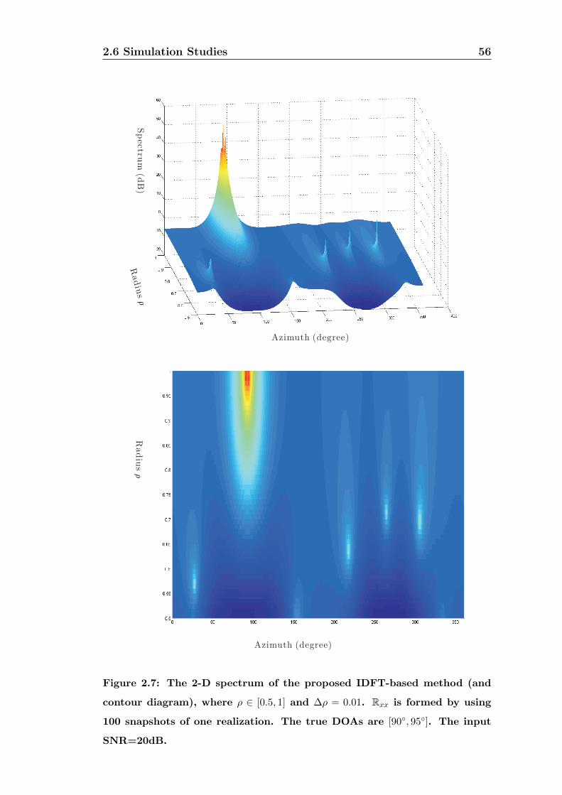
2.7 The 2-D spectrum of the proposed IDFT-based method (and con-
tour diagram), where ρ ∈ [0.5, 1] and ∆ρ = 0.01. Rxx is formed
by using 100 snapshots of one realization. The true DOAs are
[90, 95]. The input SNR=20dB. . . . . . . . . . . . . . . . . . . 56
List of Figures 11
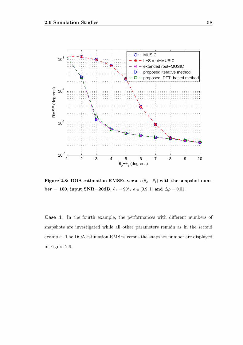
2.8 DOA estimation RMSEs versus (θ2−θ1) with the snapshot number
= 100, input SNR=20dB, θ1 = 90, ρ ∈ [0.9, 1] and ∆ρ = 0.01. . . 58
2.9 DOA estimation RMSEs versus the snapshot number with input
SNR=20dB, DOAs=[90, 95], ρ ∈ [0.9, 1] and ∆ρ = 0.01. . . . . . 59
2.10 DOA estimation RMSEs versus the input SNR with
DOAs=[90, 95], the snapshot number =100, ρ ∈ [0.9, 1]
and ∆ρ = 0.01. . . . . . . . . . . . . . . . . . . . . . . . . . . . . 60
3.1 The GSC structure of the multirank MVDR beamformer . . . . . 71
3.2 Array output SNIR versus the azimuth of the 2nd interference. The
1st interference remains at 100. The actual DOA of the desired
signal is 90 while the presumed DOA is 87. . . . . . . . . . . . . 80
3.3 Array output SNIR versus the azimuth of the 2nd interference.
The 1st interference remains at 97. The actual DOA of the desired
signal is 90 while the presumed DOA is 87. . . . . . . . . . . . . 82
3.4 Array output SNIR versus the input SNR. The two interference
DOAs are at [80, 100]. The actual DOA of the desired signal is
90 while the presumed DOA is 87. All signals are equally powered. 82
3.5 Array output SNIR versus the nominal signal subspace dimension.
The true dimension is 3. The actual DOA of the desired signal is
90 while the presumed DOA is 87. The DOAs of interferences
are [80, 100]. . . . . . . . . . . . . . . . . . . . . . . . . . . . . . 84
3.6 Array output SNIR versus the snapshot number. The actual DOA
of the desired signal is 90 while the presumed DOA is 87. The
DOAs of interferences are [80, 100]. . . . . . . . . . . . . . . . . 84
3.7 RMSE of the desired manifold versus the snapshot number. The
interference signals are from [80, 100]. The actual DOA of the
desired signal is 90 while the presumed DOA is 87. . . . . . . . 85

List of Figures 12
4.1 Decomposition of the space spanned by the columns of the data
covariance matrix when the desired signal is present . . . . . . . . 91
4.2 Decomposition of the space spanned by the columns of the data
covariance matrix when the desired signal is absent . . . . . . . . 95
4.3 The structure of the beamformer using blocking matrix . . . . . . 102
4.4 An example of spatial blocking filter with q = 1 . . . . . . . . . . 103
4.5 Illustration of the convergence of the VSP method. The point-A
represents the nominal manifold. The point-B represents the true
manifold. . . . . . . . . . . . . . . . . . . . . . . . . . . . . . . . 107
4.6 Decomposition of the space by the columns of Ri+n . . . . . . . . 114
4.7 Array pattern with two interferences close together (60 and 62).
The DOA of the desired signal is 90. . . . . . . . . . . . . . . . . 117
4.8 Effects of pointing errors with noise level at -10dB. The true di-
rection of the desired signal maintained at 90. . . . . . . . . . . 118
4.9 Effects of pointing errors. The true direction of the desired signal
maintained at 90. . . . . . . . . . . . . . . . . . . . . . . . . . . 120
4.10 The effect of finite snapshots. The true direction of the desired
signal maintained at 90. The pointing angle is 88. . . . . . . . . 121

13
List of Tables
2.1 The roots of the extended root-MUSIC and the proposed iterative
fast root-MUSIC when the theoretical covariance matrix Rxx is used. 53
2.2 (ρ, θ) pairs of the peaks of LS-root-MUSIC and the proposed IDFT-
based method when the theoretical covariance matrix Rxx is used. 53
2.3 The roots of the extended root-MUSIC and the proposed iterative
fast root-MUSIC when the covariance matrix Rxx is formed by
using 100 snapshots of one realization. . . . . . . . . . . . . . . . 57
2.4 (ρ, θ) pairs of the peaks of LS-root-MUSIC and the proposed IDFT-
based method when the covariance matrix Rxx is formed by using
100 snapshots of one realization. . . . . . . . . . . . . . . . . . . . 57
4.1 Estimated power of the desired signal . . . . . . . . . . . . . . . . 117
4.2 SNIRout (unit: dB) with noise level at -10dB . . . . . . . . . . . . 119
14
Abbreviations
AWGN additive white Gaussian noise
DL diagonal loading
DOA direction-of-arrival
FD Fourier domain
GSC generalized sidelobe canceller
IDFT inverse discrete Fourier transform
IS interference subspace
MDB matched direction beamformer
ML maximum likelihood
MST manifold separation technique
MUSIC multiple Signal Classification
MVDR minimum-variance-distionless-response
RCB robust Capon beamformer
SNIR signal-to-noise-plus-interference ratio
SNR signal-to-noise ratio
SSP signal-subspace projection
ULA uniform linear arrays
VSP vector space projections
15
Chapter 1
Introduction
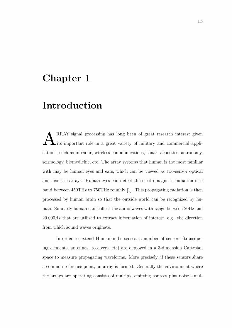
ARRAY signal processing has long been of great research interest given
its important role in a great variety of military and commercial appli-
cations, such as in radar, wireless communications, sonar, acoustics, astronomy,
seismology, biomedicine, etc. The array systems that human is the most familiar
with may be human eyes and ears, which can be viewed as two-sensor optical
and acoustic arrays. Human eyes can detect the electromagnetic radiation in a
band between 450THz to 750THz roughly [1]. This propagating radiation is then
processed by human brain so that the outside world can be recognized by hu-
man. Similarly human ears collect the audio waves with range between 20Hz and
20,000Hz that are utilized to extract information of interest, e.g., the direction
from which sound waves originate.
In order to extend Humankind’s senses, a number of sensors (transduc-
ing elements, antennas, receivers, etc) are deployed in a 3-dimension Cartesian
space to measure propagating waveforms. More precisely, if these sensors share
a common reference point, an array is formed. Generally the environment where
the arrays are operating consists of multiple emitting sources plus noise simul-

1.1 The Fundamentals of Array Signal Processing 16
taneously. Besides the desired signal(s), the other sources are referred to as
interference signals. Under certain circumstances there exist jammers that are
deliberately devised to elude the array system.
An array is utilized to sample the propagating waveforms spatially and
temporally. Then the information collected at different sensors is merged intelli-
gently so as to address the following inter-related general problems: [1, 2]
1. Parameter estimation problem — where the number and direction-of-arrival
(DOA) of the incident signals are of great interest. Essentially, the number
and DOAs are, respectively, the spatial analogues of model order selection
and frequency estimation in time-series analysis.
2. Interference cancellation — the reproduction of the desired signal from a
particular direction and the cancellation of the unwanted interferences (or
jammers), from all other directions, as much as possible.
3. Tracking — where the target sources are moving in space. The tracking
algorithms aim at determining the source location and motion over a long
period. Generally Kalman filter and its extended versions are useful to deal
with tracking problems.
In this thesis, the emphasis are placed on the DOA estimation and interference
cancellation.
1.1 The Fundamentals of Array Signal Process-
ing
The “core” of any array application is the structure of the array, which is com-
pletely characterized by the array manifold [2]. The array manifold is defined

1.1 The Fundamentals of Array Signal Processing 17
as the locus of the all response vectors, by means of which one or more real di-
rectional parameters are mapped to a (N × 1) complex vector (where N is the
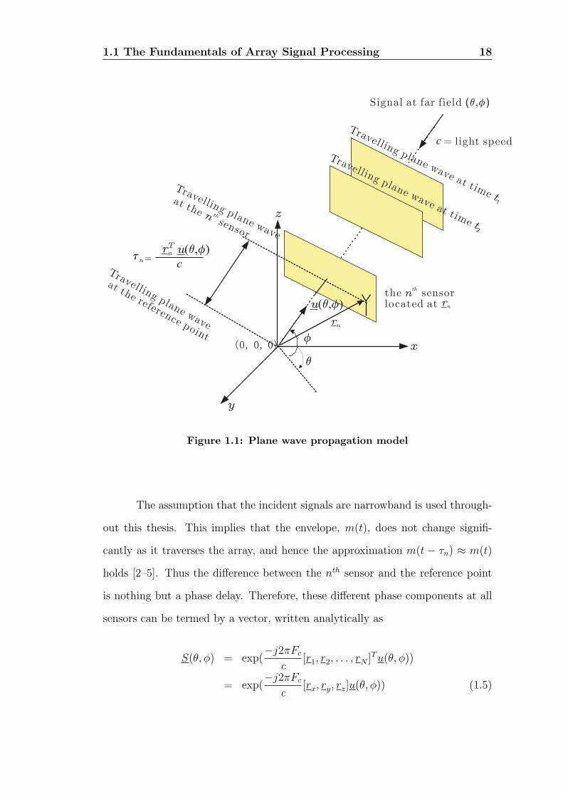
number of sensors). As shown in Figure 1.1, a signal source is located at the
far field of the array and the plane wave can be considered to model the wave
propagation. The directions of the propagating wave are termed as the azimuth
angle θ ∈ [0, 2π), measured anticlockwise from the x-axis, and the elevation angle
ϕ ∈ [0, π), measured anticlockwise from the x-y plane. Then the received signal
at the zero-phase reference point (or the original point) can be expressed as
signal at the reference point: m(t) exp(j2πFct) (1.1)
where m(t) denotes the complex envelope of the signal and exp(j2πFct) stands
for the carrier. Note that all the sensors are assumed to be isotropic, meaning
that the sensor gain is identical at all directions. The propagation delay between
the reference point and the nth sensor is given by [2]
τn =rTnu(θ, ϕ)
c(1.2)
where rn = [xn, yn, zn]T ∈ R3×1 represents the Cartesian coordinates associated
with the nth sensor, c is the wave propagation speed, say light speed, and u(θ, ϕ)
is a unit-norm vector pointing towards the propagation direction (θ, ϕ), i.e.,
u(θ, ϕ) = [cos θ cosϕ, sin θ cosϕ, sinϕ]T (1.3)
Based on the above, the signal received at the nth sensor can be expressed as
signal at the nth sensor: m(t− τn) exp(j2πFc(t− τn)) (1.4)
which is a delayed version of the signal collected at the reference point.
1.1 The Fundamentals of Array Signal Processing 18
c
u( )q f
c
(0, 0, 0)
q
Signal at far field ( )q f
Travelling plane wave at time t1
Travelling plane wave at time t2
= light speed
Travelling plane wave
at thesensor
n th
Travelling plane wave
at the reference point
the sensorlocated at
nth
fx
y
z
rn
u( )q frn
T
=tn
rn
Figure 1.1: Plane wave propagation model
The assumption that the incident signals are narrowband is used through-
out this thesis. This implies that the envelope, m(t), does not change signifi-
cantly as it traverses the array, and hence the approximation m(t − τn) ≈ m(t)
holds [2–5]. Thus the difference between the nth sensor and the reference point
is nothing but a phase delay. Therefore, these different phase components at all
sensors can be termed by a vector, written analytically as
S(θ, ϕ) = exp(−j2πFc
c[r1, r2, . . . , rN ]
Tu(θ, ϕ))
= exp(−j2πFc
c[rx, ry, rz]u(θ, ϕ)) (1.5)
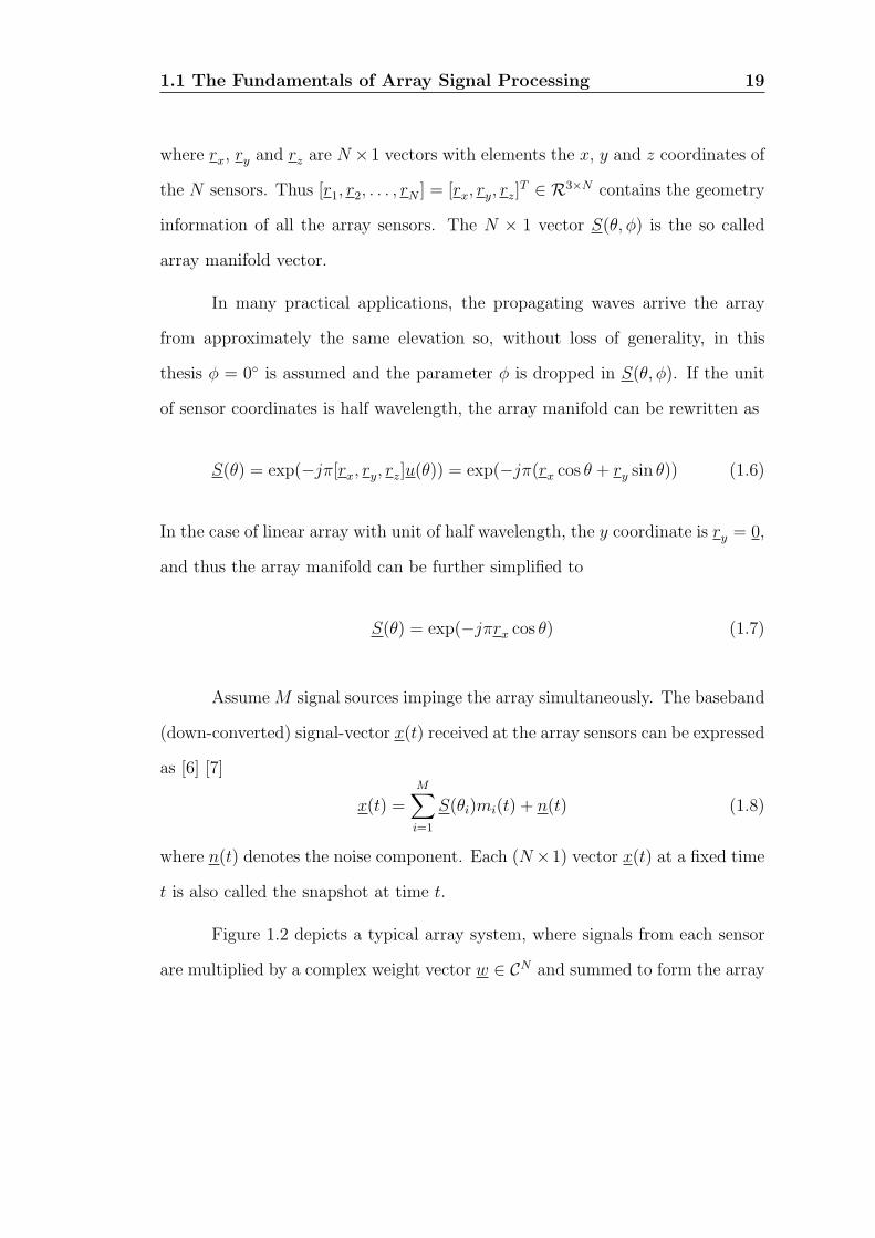
1.1 The Fundamentals of Array Signal Processing 19
where rx, ry and rz are N ×1 vectors with elements the x, y and z coordinates of
the N sensors. Thus [r1, r2, . . . , rN ] = [rx, ry, rz]T ∈ R3×N contains the geometry
information of all the array sensors. The N × 1 vector S(θ, ϕ) is the so called
array manifold vector.
In many practical applications, the propagating waves arrive the array
from approximately the same elevation so, without loss of generality, in this
thesis ϕ = 0 is assumed and the parameter ϕ is dropped in S(θ, ϕ). If the unit
of sensor coordinates is half wavelength, the array manifold can be rewritten as
S(θ) = exp(−jπ[rx, ry, rz]u(θ)) = exp(−jπ(rx cos θ + ry sin θ)) (1.6)
In the case of linear array with unit of half wavelength, the y coordinate is ry = 0,
and thus the array manifold can be further simplified to
S(θ) = exp(−jπrx cos θ) (1.7)
AssumeM signal sources impinge the array simultaneously. The baseband
(down-converted) signal-vector x(t) received at the array sensors can be expressed
as [6] [7]
x(t) =M∑i=1
S(θi)mi(t) + n(t) (1.8)
where n(t) denotes the noise component. Each (N×1) vector x(t) at a fixed time
t is also called the snapshot at time t.
Figure 1.2 depicts a typical array system, where signals from each sensor
are multiplied by a complex weight vector w ∈ CN and summed to form the array

1.1 The Fundamentals of Array Signal Processing 20
output y(t), i.e.,
y(t) = wHx(t)
=M∑i=1
wHS(θi)mi(t) + wHn(t) (1.9)
where the first term of the right hand side denotes the operation of the beam-
former on the manifold vectors, and the second term the operation on the noise.
Array ofsensors Array output
certain performance criterion
⊗N
x( )t xy t t( ) ( )=wH
w
WeightFormingAlgorithm
Figure 1.2: General block diagram of an array system
A number of strategies have been developed to form the weight vector
so as to fulfil the required criteria. For instance, maximization of the array
output signal-to-noise-plus-interference ratio (SNIR) may be the most popular
measurement for the weight design. The general idea is to let the desired signal,
at a particular direction (which is a known priori or can be estimated), pass
through unchanged, and the unwanted interference signals be suppressed as much
as possible, such that the output SNIR is as large as possible. Consequently, the
associated beam pattern presents a peak at the direction of the desired signal and
nulls at the directions of interferences. This process is also known as beamforming.

1.2 Pointing Errors 21
For processing wideband signals, a tapped-delay-line (TDL) structure is used in
the beamformer normally [7].
1.2 Pointing Errors
In practical applications, the actual DOA associated with the desired signal often
differs from the presumed (or nominal) one used by the array processor, which
leads to
S(θd) = S(θ0) with θd = θ0 (1.10)
where θd and θ0, respectively, denote the actual and nominal DOA of the desired
signal. This problem is known as the “pointing error” problem. It has been shown
in [8] that even a slight mismatch between θd and θ0 may result in substantial
performance degradation of the conventional adaptive array processor. Let us
look at an example. Assume a uniform linear array (ULA) with N = 10 sensors
and half-wavelength sensor spacing operates in the presence of three source signals
where one is the desired signal with DOA θd = 90 and two are interferences with
DOAs [60, 70]. All three signals have powers equal to one while the noise power
is 0.1. The output SNIR of the conventional adaptive array beamformer against
the pointing angle (or the presumed DOA) is plotted in Figure 1.3. It can be
seen that in this example the conventional adaptive beamformer fails even when
the pointing error is only 1.

1.3 Research Objectives and Thesis Organization 22
85 86 87 88 89 90 91 92 93 94 950
2
4
6
8
10
12
14
16
18
20
Azimuth of the presumed DOA of the desired signal
Arr
ay O
utpu
t SN
IR (
dB)
Figure 1.3: Effects of pointing errors. The true DOA of the desired signal
is 90
1.3 Research Objectives and Thesis Organiza-
tion
The primary objective of this thesis is to propose new DOA estimation algorithms
and beamformers, robust to pointing errors. The methods developed aim at
the applications at the receiver end. Throughout this thesis, it is assumed that
the incident signals are located at the far field of the array, and all signals are
uncorrelated to each other.
The rest of this thesis contains three technical chapters (Chapter 2, 3 and
4). In Chapter 2, two subspace based DOA estimation algorithms are briefly intro-
duced, in which the root-MUSIC is better than the MUltiple Signal Classification
(MUSIC) method because root-MUSIC does not suffer the grid error (and hence
1.3 Research Objectives and Thesis Organization 23
reduces point errors) while MUSIC does. In order to extend the root-MUSIC
designed for uniform linear arrays (ULA) to arbitrary arrays, however, the cost
of computational complexity is also increased. For the purpose of reducing the
complexity of the extended root-MUSIC, two computationally efficient algorithms
are proposed. In the first method, only a few largest eigenvalues corresponding
to the desired roots are needed to calculate. The second method transforms the
polynomial into a form of inverse discrete Fourier transform (IDFT) and thus
the rooting process is replaced with the operation of scanning multiple circles in
parallel. Both proposed methods achieve the same performance as the extended
root-MUSIC, but with less computational burden.
Due to a host of practical reasons, the exact knowledge of the manifold
of the desired signal is often unavailable. Chapter 3 introduces a model of the
desired signal, in which the manifold is assumed to lie in a known linear sub-
space whereas how the bases of this linear subspace are combined to form the
manifold is unknown. Two different linear subspaces are discussed which can
accommodate pointing errors. It proves that the associated linear combination
vector is able to be found by computing the principal eigenvector of a certain ma-
trix which is designed without recourse to the interference subspace. Then a so
called matched direction beamformer is constructed, which is robust to pointing
errors and overestimation of the signal subspace dimension.
In Chapter 4, the conventional Wiener-Hopf and the “modified” Wiener-
Hopf beamformers are analyzed from the standpoint view of subspace. It is
found that the Wiener-Hopf processors suffer from the problems of the power
inversion and lacking robustness to pointing errors. The “modified” Wiener-Hopf
beamformers overcome these two problems by removing the desired signal effects.
However both processors allow the interferences to pass through. The proposed

1.3 Research Objectives and Thesis Organization 24
method employs the technique of vector space projections to eliminate much of
the pointing errors. Then the power of the desired signal is estimated in a one-step
operation. The desired-signal-absent covariance matrix is formed by subtracting
the effects of the desired signal from the desired-signal-present covariance matrix.
Thus a weight vector orthogonal to the interferences can be formed. The proposed
beamformer provides a unified solution to the problems of the power inversion,
the robustness to pointing errors, and the complete interference cancellation.
Finally, in Chapter 5 the thesis is concluded and a list of the original
contributions as well as an outlook on future research are provided.

25
Chapter 2
Fast root-MUSIC for Arbitrary
Arrays
DIRECTION-OF-ARRIVAL (DOA) estimation is an ubiquitous task in
many array signal processing applications. Among the classic DOA esti-
mation techniques, maximum likelihood (ML) methods have the reputation of the
best estimation performance because they asymptotically approach the Cramer-
Rao lower bound [9]. However, their computational complexity is usually pro-
hibitive since a multi-dimensional search is needed to find the global maximum
of the likelihood function [10]. One solution to simplify the computational com-
plexity of ML methods while maintaining the high-resolution DOA estimation
ability is to use the methods called subspace methods. The MUltiple Signal
Classification (MUSIC) algorithm, invented by Schmidt [11, 12], is the first and
maybe the most popular subspace method. MUSIC searches a reduced parameter
space and in turn can be implemented with much less complexity as compared
to the ML methods [10]. However, MUSIC still requires a spectral search pro-
cess, the computational task of which may be unaffordable for some real-time
implementations [10, 13]. In order to further reduce the computational complex-
2. Fast root-MUSIC for Arbitrary Arrays 26
ity, the search-free DOA estimation methods have been developed, which aim
to avoid the spectral search step. The estimation of signal parameters via rota-
tional invariance techniques (ESPRIT), proposed in [14], employs two identical,
translationally invariant subarrays to estimate DOA, where the property that
the signal subspaces of the two subarrays are shift-invariant is used. However, it
has been shown in [15] that ESPRIT is statistically less efficient than MUSIC.
Additionally, ESPRIT seriously suffers from the calibration errors which results
in the discrepancy between the subarrays and in turn degrades the estimation
performance. Another search-free approach is the root-MUSIC, proposed in [16],
where the DOA estimation problem is reformulated as a polynomial rooting prob-
lem. In comparison with MUSIC, root-MUSIC not only substantially reduces the
computational complexity but also improves threshold performance [17]. Unfortu-
nately these search-free methods are applicable only to specific array geometries.
For instance, ESPRIT requires the subarrays with shift-invariant structure, and
root-MUSIC is designed for ULA or the non-uniform arrays whose sensors lie on
a uniform grid.
By using the manifold separation [18–20] or Fourier Domain root-MUSIC
techniques [13], root-MUSIC has been extended to arrays with arbitrary geome-
try but at the cost of increased computational complexity. In this chapter, two
fast algorithms are presented to reduce the computational cost. The first pro-
posed method is implemented in an iterative way where the Schur algorithm [21]
is conducted to factorize the Laurent structured polynomial. Then Arnoldi it-
eration [22] is employed to compute only a few of the largest eigenvalues. This
implies that a large number of the unwanted eigenvalues (or roots) are exempt
from the calculation and therefore the computational complexity is reduced sig-
nificantly. The second approach has a work-efficient parallel implementation, in
2.1 Background of Subspace DOA Estimation 27
which inverse discrete Fourier transform (IDFT) is used and polynomial rooting
is avoided. Both proposed methods, with less computational burden, asymptoti-
cally exhibit the same performance as the extended root-MUSIC, implying that
they outperform the conventional MUSIC in terms of resolution ability.
2.1 Background of Subspace DOA Estimation
Let an array with N omnidirectional sensors receive M narrowband signals lo-
cated in the far field. The N × 1 array snapshot vector at time t can be modeled
as
x(t) =M∑i=1
S(θi)mi(t) + n(t) (2.1)
where n(t) ∈ CN is a complex noise vector which corrupts the received sig-
nal. Here it assumes that the noise is zero-mean additive white Gaussian noise
(AWGN) and uncorrelated from sensor to sensor. It is also assumed that the sig-
nals are uncorrelated with each other and with the noise. Using matrix notation,
the received snapshot vector may be rewritten in a compact form
x(t) = Sm(t) + n(t) (2.2)
where m(t) = [m1(t), . . . ,mM(t)]T ∈ CM stands for the vector of M complex
narrowband signal envelopes. The N ×M matrix S has columns the manifold
vectors of the M signals, i.e.,
S = [S(θ1), . . . , S(θM)] (2.3)

2.1 Background of Subspace DOA Estimation 28
which is assumed to be of full column rank meaning that N > M . The second
order statistics of the vector-signal x(t) is represented by the covariance matrix
Rxx
Rxx = Ex(t)xH(t)
= SRmmSH + σ2
nIN (2.4)
where σ2n denotes the power of the AWGN noise. The covariance matrix of signals
is represented by Rmm which, under the assumption of uncorrelated signals, is
given by
Rmm = Em(t)mH(t)
=
σ21, 0, . . . , 0
0, σ22, . . . , 0
......
. . ....
0, 0, . . . , σ2M
(2.5)
where σ2i = Em2
i (t) is the power of the ith signals. Performing eigen-
decomposition on Rxx gives
Rxx =N∑i=1
λiEiEHi (2.6)
where the eigenvalues λi, i = 1, . . . , N are arranged in nonascending order (i.e.,
λ1 ≥ . . . ≥ λN), and Ei is the eigenvector corresponding to λi. Theoretically, the
smallest N −M eigenvalues are equal to the noise power, i.e.,
λM+1 = . . . = λN = σ2n (2.7)
Then Rxx may be partitioned into two parts as follows
Rxx = Es(Ds + σ2nIM)EH
s + σ2nEnEH
n (2.8)
2.1 Background of Subspace DOA Estimation 29
where the diagonal matrix Ds is defined as
Ds =
λ1 − σ2n, 0, . . . , 0
0, λ2 − σ2n, . . . , 0
......
. . ....
0, 0, . . . , λM − σ2n
(2.9)
Es and En contain, respectively, the eigenvectors associated with the largest M
eigenvalues (or the first M dominant eigenvectors) and the remaining eigenvec-
tors, i.e.,
Es= [E1, E2, . . . , EM ]
En= [EM+1, EM+2, . . . , EN ] (2.10)
Also, Es and En are referred to as signal- and noise-subspace eigenvectors.
It is well known that the subspace spanned by Es is equal to that spanned
by S [11,12]. Moreover, the signal subspace is orthogonal to the noise subspace. In
mathematics, the relationship among these three subspace is expressed as follows
L[Es] = L[S]⊥L[En] (2.11)
In practical applications, the exact covariance matrix Rxx is unavailable
and its sample estimate below is used.
Rxx =1
L
L∑l=1
x(tl)xH(tl) (2.12)
where x(tl) denotes the snapshot vector received at time tl and L is the number
of the snapshots. For this case, the mean of the N −M smallest eigenvalues is

2.1 Background of Subspace DOA Estimation 30
used to estimate σ2n, i.e.,
σ2n =
N∑i=M+1
λ2i
N −M(2.13)
2.1.1 Classical MUSIC
Due to the orthogonality between the signal and noise subspace, the angles where
the projection of the corresponding manifold onto the noise subspace are zero
should be the DOAs of signals. By exploiting this property, the MUSIC searches
the continuous array manifold vector S(θ) over the area of θ to find theM minima
of the following null-spectrum function
ξ(θ) = SH(θ)EnEHn S(θ) = ∥EH
n S(θ)∥2 (2.14)
The major drawbacks associated with MUSIC are:
1. The estimation error due to “grid” based search may occur. For instance, if
the array manifold is searched in the step of 1, the signal located at 10.5
may be not found. This grid error (or quantization error) definitely causes
pointing error of the manifold vector [23].
2. The computational complexity is high, particularly for the real-time appli-
cations, which can be explained by the following fact. For the purpose of
avoiding grid error, the required number of search points has to be signifi-
cantly large. In other words, the angular search grid has to be fine enough to
avoid the quantization problem [23]. To obtain each search point, moreover,
a matrix product of EHn and S(θ) and the associated norm (see Eq.(2.14))
have to be computed.

2.1 Background of Subspace DOA Estimation 31
2.1.2 Root-MUSIC
Suppose the array used is a ULA array, then the associated y and z coordinates
of array sensors become ry = rz = 0, and the x coordinate is expressed as
rx = [0,D, . . . ,DN−1]T (2.15)
where the first sensor is chosen as the reference point, and D stands for the
distance between the adjacent sensors which is usually half wavelength. Now the
corresponding manifold vector can be written as follows
S(θ) = exp(−jπrx cos θ) = [1, z, . . . , zN−1]T (2.16)
where z is defined as
z = exp(−jπD cos θ) (2.17)
Clearly the manifold in Eq.(2.16) is Vandermonde structured. Using the fact
that z∗ = 1/z (where (·)∗ denotes the complex conjugate operation), the MUSIC
null-spectrum function can be rewritten as follows
ξ(z) = SH(θ)EnEHn S(θ)
= [1,1
z, . . . ,
1
zN−1]EnEH
n [1, z, . . . , zN−1]T
=N−1∑
i=−N+1
biz−i (2.18)
where the coefficient bi is the sum of the elements of the matrix EnEHn along the
ith diagonal, i.e.,
bi =∑
∀m−n=i
[EnEHn ]m,n (2.19)
2.1 Background of Subspace DOA Estimation 32
where the notation [A]m,n denotes the (m,n)th entry of the matrix A. Clearly, ξ(z)
is a univariate polynomial with degree of (2N − 2). The DOAs of the M signals
are corresponding to the roots of ξ(z). Thus the DOA estimation is reduced to a
root finding problem, in which DOAs can be obtained as the phase angles of the
roots closest to the unit circle.
Instead of searching over θ, the root version MUSIC overcomes the quan-
tization problem and high computational complexity aforementioned in the MU-
SIC. Another favorable advantage of root-MUSIC over classical MUSIC is that
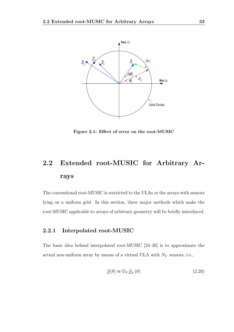
root-MUSIC is immune to radial errors [17]. As shown in Figure 2.1, if the er-
ror ∆zi is along the radial direction, there is no error in the DOA estimation
(i.e., ∆θi = 0). Nevertheless, such radial error affects the MUSIC because MU-
SIC searches the unit circle only. In Figure 2.1, it is illustrated that two closely
spaced roots z1 and z2 , due to radial error, may correspond to a common point
z3 on the unit circle. In such case, the resulting MUSIC angular spectrum has
only one peak which causes an apparent loss in resolution, and hence the point
error occurs, no matter how fine the search grid is.
2.2 Extended root-MUSIC for Arbitrary Arrays 33
Unit Circle
∆iz
iz
iθ
i∆θ
Im( )z
Re( )z
iz
1z
2z
3z
Figure 2.1: Effect of error on the root-MUSIC
2.2 Extended root-MUSIC for Arbitrary Ar-
rays
The conventional root-MUSIC is restricted to the ULAs or the arrays with sensors
lying on a uniform grid. In this section, three major methods which make the
root-MUSIC applicable to arrays of arbitrary geometry will be briefly introduced.
2.2.1 Interpolated root-MUSIC
The basic idea behind interpolated root-MUSIC [24–26] is to approximate the
actual non-uniform array by means of a virtual ULA with NV sensors, i.e.,
S(θ) ≈ GV SV (θ) (2.20)

2.2 Extended root-MUSIC for Arbitrary Arrays 34
where SV (θ) is the NV × 1 manifold vector of the virtual ULA. Note that the
dimension of the virtual array manifold is less than that of the actual manifold,
i.e., NV ≤ N . The “thin” matrix GV ∈ CN×NV is the interpolation matrix
designed to minimize the interpolation error. Using the above approximation,
the null-spectrum of interpolated root-MUSIC can be defined as
ξintp = SHV (θ)GH
V EnEHn GV SV (θ) (2.21)
Apparently, the above null-spectrum has similar form with the standard root-
MUSIC null-spectrum (see Eq.(2.18)) and thus the conventional root-MUSIC
algorithm can be applied on it.
The main problem of interpolation root-MUSIC is that the approximation
in Eq.(2.20) often introduces significant mapping errors which may cause DOA
estimation bias and excess variance [27]. Another problem is that the approxi-
mation is inaccurate for the whole angular field-of-view, which implies that the
mapping matrix GV is dependent on angular sector. Hence in the practical im-
plementation, the information that which sector the DOAs belong to has to be
given or estimated. The next two approaches avoid these two problems.
2.2.2 Manifold Separation Technique (MST)
The nth element of the manifold vector, denoted by [S(r, θ)]n, can be explicitly
written as a function of both array geometry and DOA as follows
[S(r, θ)]n = exp(−jπrTnu(θ)
)= exp (−jπ(xn cos θ + yn sin θ))
= exp (−jπ∥rn∥ cos(ψn − θ)) (2.22)

2.2 Extended root-MUSIC for Arbitrary Arrays 35
where (xn, yn) denotes the x-y coordinates of the nth sensor in units of half wave-
length, and (∥rn∥, ψn) represents the corresponding polar coordinates, which is
given by
∥rn∥ =√x2n + y2n
ψn = tan−1
(ynxn
)(2.23)
By using the Jacobi-Anger expansion [28], [S(r, θ)]n can be written as
[S(r, θ)]n =∞∑
q=−∞
jqJq(−π∥rn∥) exp(jq(ψn − θ))
=∞∑
q=−∞
jqJq(−π∥rn∥) exp(jqψn) exp(−jqθ) (2.24)
Thus the manifold vector S(r, θ) can be written as
S(r, θ) =∞∑
q=−∞
jq
Jq(−π∥r1∥)
Jq(−π∥r2∥)...
Jq(−π∥rN∥)
⊙
exp(jqψ1)
exp(jqψ2)
...
exp(jqψN)
︸ ︷︷ ︸
=Gq∈CN
exp(−jqθ) (2.25)
where ⊙ denotes the operation of Hadamard product (or elementwise product).
By ignoring the terms with q greater than ±Q (where Q= NV −1
2), the manifold
vector S(r, θ) may be rewritten as
S(r, θ) = G(r)d(θ) + ε (2.26)

2.2 Extended root-MUSIC for Arbitrary Arrays 36
where G(r) ∈ CN×NV , dependent on the array geometry only, is defined as
G(r) =
[G−Q, G−Q+1, · · · , GQ−1 GQ
]∈ CN×NV (2.27)
with Gq ∈ CN defined in Eq.(2.25). The Vandermonde structured vector d(θ) ∈
CNV is dependent on the azimuth only and has the following form
d(θ) =
[Z−Q, Z−Q+1, · · · , ZQ−1, ZQ
]T∈ CNV (2.28)
with
Z = exp(−jθ) (2.29)
ε represents the truncation error, which decays superexponentially as NV in-
creases and tends to zero as NV → ∞ [18]. This means that the vector ε can
be safely neglected without generating significant modeling errors, provided that
NV is sufficiently large (generally NV ≫ N). Note that only the azimuth angle
θ ∈ [0, 360) is considered in this thesis. For the 2-D case (azimuth and elevation
estimation problem), spherical harmonics is used to model d(θ, ϕ) [18].
Under the condition that NV is large enough such that ε can be safely
neglected, a polynomial is constructed as follows
ξ(Z) = SH(r, θ)EnEHn S(r, θ)
= dH(θ)GH(r)EnEHn G(r)d(θ)
=1
2π
NV −1∑i=−(NV −1)
biZ−i (2.30)
where the coefficient bi is the sum of entries of GH(r)EnEHn G(r) ∈ CNV ×NV along
2.2 Extended root-MUSIC for Arbitrary Arrays 37
the ith diagonal, i.e.,
bi =∑
∀m−n=i
[GH(r)EnEHn G(r)]m,n (2.31)
ξ(Z) is a polynomial with degree of (2NV − 2), meaning that there are (2NV − 2)
roots. M roots closest to the unit circle should be selected among the (2NV − 2)
roots and the phase angles of the M roots are utilized to estimate the DOAs.
2.2.3 Fourier Domain (FD) root-MUSIC
In [13], a competitive alternative to the MST, called Fourier Domain (FD) root-
MUSIC, has been proposed. The MUSIC null spectrum function Eq.(2.14) is
periodic in θ with period 2π, because S(θ) = S(θ + 2π). Therefore, the null
spectrum can be rewritten by Fourier series expansion as
ξ(θ) =∞∑
i=−∞
biejiθ =
∞∑i=−∞
biZ i (2.32)
with
Z =exp(jθ) (2.33)
The Fourier coefficients are obtained by
bi =1
2π
∫ π
−π
ξ(θ)Z−idθ (2.34)
Here the null spectrum function ξ(θ) over the angular domain may be analogous to
the conventional signal function over time domain. Similar to MST, the function
ξ(θ) can be truncated to finite dimension as
ξ(θ) ≈NV −1∑
i=−(NV −1)
biZ i (2.35)

2.2 Extended root-MUSIC for Arbitrary Arrays 38
where
bi ≈1
2π
NV −1∑k=−(NV −1)
ξ(k∆θ)e−jik∆θ
=1
2π
NV −1∑k=−(NV −1)
∥∥EHn S(k∆θ)
∥∥2 e−jik∆θ (2.36)
with
∆θ =2π
2NV − 1(2.37)
The coefficients bi can be expressed in a compact matrix form as follows
b =
[b−(NV −1), b−(NV −2), . . . , b(NV −1)
]T= FB (2.38)
where
F =1
2π
e−j(NV −1)(NV −1)∆θ, e−j(NV −1)(NV −2)∆θ, . . . ej(NV −1)(NV −1)∆θ
e−j(NV −2)(NV −1)∆θ, e−j(NV −2)(NV −2)∆θ, . . . ej(NV −2)(NV −1)∆θ
......
. . ....
ej(NV −1)(NV −1)∆θ, ej(NV −1)(NV −2)∆θ, . . . e−j(NV −1)(NV −1)∆θ
(2.39)
and
B =
∥∥EHn S(−(NV − 1)∆θ)
∥∥2∥∥EHn S(−(NV − 2)∆θ)
∥∥2...∥∥EH
n S((NV − 1)∆θ)∥∥2
∈ R2NV −1 (2.40)
Now the FD root-MUSIC may be implemented via the following steps:
1. Compute (2NV − 1) MUSIC spectral points ξ(k∆θ), k = −(NV −
1), . . . , NV − 1.
2. Calculate the (2NV − 1) Fourier coefficients bi using Eq.(2.36) where the

2.2 Extended root-MUSIC for Arbitrary Arrays 39
method of discrete Fourier transform (DFT) can be used.
3. Construct the polynomial of Eq.(2.35) whose degree is 2NV − 2, using bi.
4. Apply the root-MUSIC algorithm on this polynomial to estimate the DOAs.
Compared with MST technique, the FD root-MUSIC has achieved two
improvements. One is the computational complexity of finding the polynomial
coefficients is slightly smaller than that of MST. Another is that the DOA esti-
mation variance of the FD root-MUSIC is smaller than that of MST when the
polynomial degree is quite small. If the polynomial degree is relatively large, both
FD root-MUSIC and MST have the same estimation performance.
One common problem of the MST and FD root-MUSIC is that they need to
solve a polynomial with high degree, since the value of NV has to be sufficiently
large to restrict the truncation errors to a wanted level. The requirement of
computing all the (2NV −2) roots of (2.30) (or (2.35)), coupled with the fact that
NV is significantly large, may render the two methods computationally expensive,
particularly when the sensor number N is also very large. In [13] an IDFT-based
method, named line-search root-MUSIC, has been proposed. Nevertheless, the
resolution ability of this method is inferior to the root-based methods.
Next, two algorithms will be developed to reduce the complexity of rooting
the polynomial with high degree. It is important to point out that the proposed
algorithms are applicable to both MST and FD root-MUSIC. Moreover, the res-
olution ability of the proposed methods are asymptotically same as the extended
root-MUSIC.
2.3 Iterative Fast root-MUSIC 40
2.3 Iterative Fast root-MUSIC
Let us reexamine (2.30) and (2.35). Both of them are of Laurent polynomial [29].
Taking into account the Hermitian property of the matrix GH(r)EnEHn G(r), one
obtains the coefficients bi = b∗−i. Furthermore, the null spectrum is non-negative
because ξ(θ) = ∥EHn S(θ)∥2 ≥ 0. Since the polynomial resulted from MST is
similar with that from FD root-MUSIC, only the case of MST is discussed in the
rest of this chapter. The polynomial of (2.30) can be factorized into two parts,
which is supported by the following lemma.
Lemma 1.1 [21]: Consider a Laurent polynomial ξ(Z),
ξ(Z) =
NV −1∑i=−(NV −1)
biZ−i, with bi = b∗−i (2.41)
and such that it is non-negative on the unit circle, ξ(ejΩ) ≥ 0. Then the canonical
factorization of ξ(Z) is given by
ξ(Z) = c1ξ1(Z)ξ∗1(1/Z
∗) (2.42)
where c1 is a positive constant. The roots of ξ(Z) appear in conjugate reciprocal
pairs, i.e., if Z1 is a root of ξ(Z), then (Z−11 )∗ is also a root.
Proof: Also see [21]
Clearly the polynomial ξ(Z) in (2.30) meets the conditions of the above
lemma, which means that ξ(Z) can be factorized into two parts. Moreover,
computing half of the roots (i.e., roots of ξ1(Z)) is sufficient to find the roots of
interest. To this end, a spectral factorization method should be employed. An
excellent survey of spectral factorization methods has been provided in [21]. In
these methods, a sequence of banded Hermitian Toeplitz matrices is formed as

2.3 Iterative Fast root-MUSIC 41
follows
T0 = b0, T1 =
b0, b−1
b1, b0
, . . . ,Tk =
b0, b−1, . . . , b−k
b1, b0, . . . , b−k+1
......
. . ....
bk, bk−1, . . . , b0
(2.43)
Performing triangular factorization on Tk gives
Tk = LkDkLHk (2.44)
where Lk represents a lower triangular matrix with unit diagonal entries and Dk
is a positive diagonal matrix. As k → ∞, the last NV entries of the last row of
Lk tend exponentially fast to the coefficients of ξ1(Z) [21]. To accomplish the
triangular factorization, the computationally efficient Schur algorithm, in which
the Toeplitz structure is exploited, is employed in this thesis. The Schur method
can be implemented via the following steps:
1. Initialize a (NV × 2) matrix B0, using bi calculated from (2.31).
B0 =
b0, b−1
b−1, b−2
......
b−(NV −2), b−(NV −1)
b−(NV −1), 0
(2.45)
2. For k = 1, 2, · · · until convergence, iterate the following steps

2.3 Iterative Fast root-MUSIC 42
(a) Bk = Bk−1Uk, where Uk is a (2× 2) matrix defined as
Uk =1√
1− |γ|2
1 −γ
−γ∗ 1
(2.46)
with γ = [Bk−1]1,2/[Bk−1]1,1, i.e., the ratio of the two entries of the first
row of Bk−1.
(b) Shift up the second column of Bk by one element while keeping the
first column unaltered.
(c) Test for convergence∥∥b1,k − b1,k−1
∥∥ < threshold, where b1,k and b1,k−1
denote the first column of Bk and Bk−1 respectively. If converged, go
to (3), else return to (2.a).
3. The coefficients of ξ1(Z) are b∗1,k.
Now the polynomial factor ξ1(Z), which has all its roots on or inside the
unit circle, is split from ξ(Z). To find the roots, one can construct an unsymmetric
companion matrix M whose eigenvalues correspond to the roots of ξ1(Z). Let the
polynomial ξ1(Z) = C0+C1Z+C2Z2+. . .+CNV −1Z
NV −1. Then the corresponding
companion matrix is given by [22,30]
M =
0, 0, · · · , 0, − C0
CNV −1
1, 0, · · · , 0, − C1
CNV −1
0, 1, · · · , 0, − C2
CNV −1
......
. . ....
...
0, 0, · · · , 1, −CNV −2
CNV −1
(2.47)
The eigenvalues of interest, corresponding to the DOAs, must be the M largest
ones of M because all roots of ξ1(Z) are within the unit circle. This implies that

2.3 Iterative Fast root-MUSIC 43
only a few largest eigenvalues of M are necessary. Power method [22] is a classic
and the simplest algorithm to find the largest eigenvalue. However, the power
iteration suffers from the slow convergence when the gap between the first and
the second largest eigenvalues are not sufficiently wide [22, 31]. Also, only one
eigenvalue (the largest one) can be computed by the power method. To overcome
these two drawbacks, the methods of Lanczos iteration and Arnoldi iteration have
been proposed to find the large eigenvalues of symmetric and unsymmetric matri-
ces respectively. Here the Arnoldi iteration is employed because the companion
matrix M is an unsymmetric matrix. See Appendix 1.A for the introduction of
Arnoldi iteration. Note that the function eigs.m of MATLAB has implemented
Arnoldi iteration by using the ARPACK software package [32].
To summarize, the proposed fast iterative root-MUSIC algorithm for ar-
bitrary arrays can be accomplished via the following steps:
1. Compute the sampling matrix G(r). Note that this off-line process requires
to be done only once for a given array.
2. Form the received data covariance matrix and perform eigen-decomposition
to obtain the noise subspace vectors En. Then the coefficients of ξ(Z) can
be calculated using (2.31).
3. Perform fast spectral factorization on ξ(Z) via Schur Algorithm to obtain
the polynomial factor ξ1(Z) and the corresponding companion matrix M.
4. Apply Arnoldi iteration method to calculate the M largest eigenvalues of
M. Then DOAs can be estimated by the phase angles of these eigenvalues.

2.4 IDFT-based root-MUSIC 44
2.4 IDFT-based root-MUSIC
In practice, the roots of (2.30) (or (2.35)) are not exactly on the unit circle any
more in the presence of perturbation, e.g, the effects of finite snapshots (finite
observation interval). Even the slightest perturbation can result in the roots
moving away from the unit circle (pp.209 of [33]). Therefore, it is reasonable to
model the roots as
Z = ρe−jθ (2.48)
where ρ denotes the radius. Following the work of [34], one can rewrite the
polynomial in (2.30) explicitly dependent on θ and ρ by substituting (2.48) into
(2.30)
ξ(θ, ρ) =1
2π
NV −1∑i=−(NV −1)
biρ−iejiθ
=1
2π
NV −1∑i=−(NV −1)
Bi(ρ)ejiθ
=1
2πej(1−NV )θ
2NV −1∑k=1
Bk−NV(ρ)ej(k−1)θ
=1
2πej(1−NV )θ
K∑k=1
Bk(ρ)ej(k−1)θ (2.49)
where Bi(ρ) , biρ−i and k , i + NV . The number K, no less than (2NV − 1),
takes the value of a power of 2. The coefficient Bk(ρ) is defined as
Bk(ρ) =
Bk−NV
(ρ), if 1 ≤ k ≤ (2NV − 1)
0, if (2NV − 1) < k ≤ K
(2.50)

2.4 IDFT-based root-MUSIC 45
Then the magnitude of (2.49) is given by
|ξ(θ, ρ)| = 1
2π
∣∣∣∣∣K∑k=1
Bk(ρ)ej(k−1)θ
∣∣∣∣∣ (2.51)
and thus a 2-D spectrum is defined as
PIDFT(n, ρ) =1∣∣∣ξ(ρ, 2π(n−1)K
)∣∣∣
=2π/K∣∣∣∣ 1K K∑
k=1
Bk(ρ)ej 2πK
(k−1)(n−1)
∣∣∣∣ (2.52)
where n = 1, 2, . . . , K. Interestingly, the denominator of the above has a typical
K-point IDFT form, meaning that the 2-D spectrum can be computed directly by
using IDFT for a given ρ. Apparently the peaks of the 2-D spectrum correspond
to the true DOAs because the roots of (2.49) are associated with the true DOAs.
The DOAs can be estimated by the follows.
θm =2π(nm − 1)
K(2.53)
where nm corresponds to the index-n of the mth peak of the 2-D spectrum
PIDFT(n, ρ).
Also, Eq.(2.52) can be rewritten in a compact form as
PIDFT = F B ∈ CK×L (2.54)
where L is the total number of circles required to scan. F ∈ CK×K is an in-
verse Fourier transform matrix and B ∈ CK×L denotes a coefficient matrix. The

2.4 IDFT-based root-MUSIC 46
elements of the three matrices in Eq.(2.54) are defined as follows
[PIDFT]n,ℓ =2π
PIDFT(n, ρℓ)(2.55a)
[F]n,k = ej2πK
(k−1)(n−1) (2.55b)
[B]n,ℓ = Bn(ρℓ) (2.55c)
Thus, finding peaks in Eq.(2.52) is equivalent to finding minima in Eq.(2.54).
In summary, the proposed IDFT-based root-MUSIC algorithm can be ac-
complished via the following steps:
1. Compute the matrix G(r) (off-line process).
2. Form the covariance matrix Rxx by using the observed snapshots and per-
form eigen-decomposition to obtain the noise subspace vectors En. Then
the coefficients bi can be calculated using (2.31).
3. For ρ = 1, 1 − ∆ρ, · · · until ρ = 1 − (L − 1)∆ρ, do the following steps to
scan the spectra along L circles inside the unit circle. ∆ρ determines the
grid of the circles.
(a) Calculate the (2NV−1) coefficientsBi(ρ) = biρ−i. Then the coefficients
Bk(ρ) can be obtained by padding Bi(ρ) with (K − 2NV + 1) zeros.
(b) Perform K-point IDFT operation on Bk(ρ) and invert the results to
obtain the spectrum PIDFT(n, ρ) in (2.52) for the current radius ρ.
4. Identify theM peaks closest to the unit circle via 2-D search on the spectra.
5. Estimate DOAs by using (2.53).
If one scans the unit circle only, i.e., ρ is fixed at 1, then the proposed
algorithm reduces to line-search root-MUSIC (LS-root-MUSIC) [13,34] similar to

2.5 Computational Complexity Analysis 47
that proposed in [13, 34]. LS-root-MUSIC is essentially identical to the conven-
tional MUSIC, except that all spectral points of LS-root-MUSIC are calculated
by one K-point IDFT operation while in MUSIC each point is obtained by a
matrix multiplication. LS-root-MUSIC and MUSIC are under the assumption
that, corresponding to each true DOA, there is a peak in the spectrum along
the unit circle. This is a stronger assumption than distinct Z-plane roots be-
cause the root-based methods are insensitive to the radial errors [17]. Hence, the
proposed IDFT-based method is expected to have better resolution ability than
LS-root-MUSIC and MUSIC.
2.5 Computational Complexity Analysis
The complexity order of the rooting in the extended root-MUSIC isO((2NV−2)3),
when assuming that eigenvalue-based methods are used for rooting. That is the
roots are found by computing the eigenvalues of the corresponding (2NV − 2)×
(2NV − 2) companion matrix. In the proposed iterative algorithm, the Schur
algorithm requires O(2N2V ) operation for the spectral factorization [35–37]. The
complexity of an Arnoldi iteration is roughly O(M2NV ) [38, 39]. Considering
the fact that M is far less than NV , the complexity of Arnoldi iteration may
be ignored compared with the Schur algorithm. Thus the proposed iterative
algorithm reduces the complexity of rooting from O((2NV − 2)3) to O(2N2V ).
The complexity order of LS-root-MUSIC is O(K log2K). Each loop of
Step 3 of the proposed IDFT-based method takes O(2NV ) operations to compute
the coefficient Bk(ρ) and O(K log2K) operations for K-point IDFT. Thus the
overall complexity order of the second proposed method isO(L(2NV +K log2K)).
Therefore, the computational complexity of the two IDFT-based methods will not
2.6 Simulation Studies 48
essentially increase when NV becomes large (e.g., in the applications of large scale
arrays), whereas the complexity of the extended root-MUSIC will suffer because it
increases cubically with NV . Note the line search or 2-D search for the two IDFT-
based methods has different meaning than the search process in the conventional
MUSIC method. In the MUSIC method, each spectral point needs an operation
of matrix production. However, in both IDFT-based methods, all spectral points
are obtained simultaneously by one IDFT operation. Furthermore, the IDFT
operation dominates the computing time and hereby the complexity of search
process is not included in the analysis here.
It is important to point out that the spectra of the L circles can be com-
puted simultaneously in parallel time O(2NV +K log2K) if using L processors,
which is comparable to that of LS-root-MUSIC. Despite the possible increase in
computational complexity, the proposed algorithms generally offer greater esti-
mation accuracy than LS-root-MUSIC.
2.6 Simulation Studies
Assume M = 2 uncorrelated equally-powered signals impinge on a non-ULA
array of N = 5 sensors. A randomly generated x-y Cartesian coordinates of
array sensors, in units of half-wavelengths, is shown below
r =
0, 0.9, 1.7, 2.6, 2.5
0, 0.3, −0.1, 0.3, −0.5
This array geometry is fixed throughout all simulation runs. The column size
of G(r) is set to be NV = 99, which provides the modeling error ∥ε∥ ≤ 10−15.
The grid of the circles is ∆ρ = 0.01. The IDFT length is K = 213 and MUSIC

2.6 Simulation Studies 49
search grid is 0.01. In the following experiments, five methods are examined:
conventional MUSIC, LS-root-MUSIC, the extended root-MUSIC, the proposed
iterative fast root-MUSIC and the proposed IDFT-based root-MUSIC.
Case 1: In the first example, the true DOAs are [90, 95] and the input SNR
is 20dB. The theoretical covariance matrix Rxx (see Eq.(2.4)) is used. Figure 2.2
shows the angular spectra of the MUSIC and LS-root-MUSIC between 50 and
130. Note that the field-of-view of this 2-D array is [0, 360) despite only the
spectrum over [50, 130] being plotted.
50 60 70 80 90 100 110 120 130
0
20
40
60
80
100
120
140
160
Azimuth (degree)
Spe
ctru
m (
dB)
MUSICLS−root−MUSICTrue DOAs
Figure 2.2: The angular spectra of MUSIC and LS-root-MUSIC using the-
oretical Rxx. The true DOAs are [90, 95]. The input SNR=20dB.
It can be seen from Figure 2.2 that the two spectrum curves almost
2.6 Simulation Studies 50
overlap perfectly, which means that the two methods are essentially identi-
cal. The two peaks of the two methods are located, respectively, at (90, 95)
and (89.96, 94.97). The estimation errors of LS-root-MUSIC is due to the
quantization-error caused by limited angular grid step (here the grid is 360/213 =
0.0439).
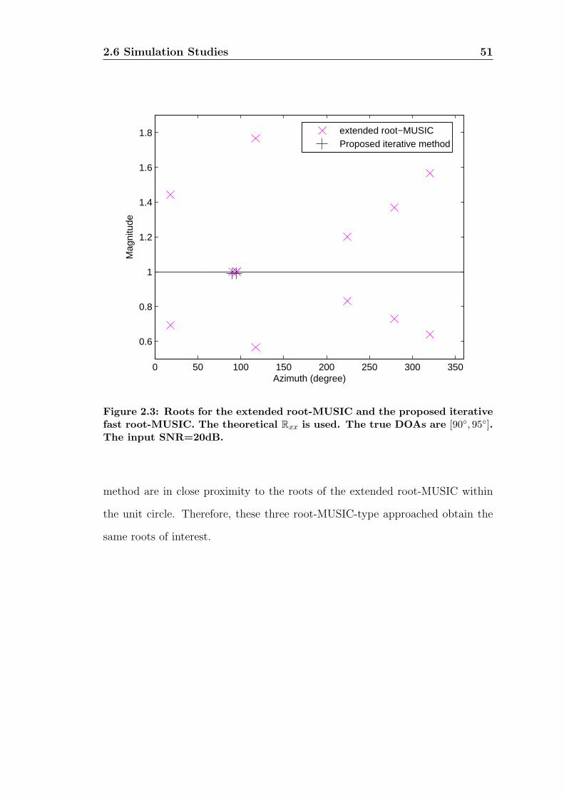
The theoretical covariance matrix is also processed by the three root-
MUSIC-type methods. In Figure 2.3, roots of the extended root-MUSIC are
plotted, along with the two roots obtained by the proposed iterative fast root-
MUSIC. Though only the roots with magnitude in the area [0.5, 2] are selected for
the extend root-MUSIC, it is enough to reveal the essence. The 2-D spectrum of
the proposed IDFT-based method is depicted in Figure 2.4 with ρ ∈ [0.5, 1] and
∆ρ = 0.01 (i.e., L=51). Note that in practice L is not required to be such a large
number because empirically ρ ∈ [0.9, 1] is sufficient to locate the true DOAs.
Our aim here is to give a more comprehensive view of the spectrum of the pro-
posed method. Figure 2.3 and 2.4 demonstrate that the three root-MUSIC-type
approaches can find the two DOAs as well.
In order to further examine the simulation results, the roots of the ex-
tended root-MUSIC and the proposed iterative method, in conjunction with the
(ρ, θ) pairs of the peaks of the two IDFT-based methods, are listed in Table 2.1
and 2.2 respectively. As shown in Table 2.1, the roots of the extended root-
MUSIC satisfy the conjugate reciprocity property. That is the roots outside and
inside the unit circle have the common phase angle but reciprocal magnitudes.
The roots computed by the proposed iterative method approximate ideally the
roots of interest by the extended root-MUSIC. In Table 2.2, it can be seen that the
peaks of LS-root-MUSIC are corresponding to the proposed IDFT-based method
with ρ = 1. Importantly, the (ρ, θ) pairs of peaks of the proposed IDFT-based
2.6 Simulation Studies 51
0 50 100 150 200 250 300 350
0.6
0.8
1
1.2
1.4
1.6
1.8
Azimuth (degree)
Mag
nitu
de
extended root−MUSICProposed iterative method
Figure 2.3: Roots for the extended root-MUSIC and the proposed iterativefast root-MUSIC. The theoretical Rxx is used. The true DOAs are [90, 95].The input SNR=20dB.
method are in close proximity to the roots of the extended root-MUSIC within
the unit circle. Therefore, these three root-MUSIC-type approached obtain the
same roots of interest.

2.6 Simulation Studies 52
Azimuth (degree)
Azimuth (degree)
Radiu
sr
Radiu
sr
Spectr
um
(dB
)
Figure 2.4: The 2-D spectrum of the proposed IDFT-based method (andcontour diagram), where ρ ∈ [0.5, 1] and ∆ρ = 0.01. The theoretical Rxx isused. The true DOAs are [90, 95]. The input SNR=20dB.

2.6 Simulation Studies 53
Table 2.1: The roots of the extended root-MUSIC and the proposed itera-tive fast root-MUSIC when the theoretical covariance matrix Rxx is used.
extended root-MUSIC proposed iterative fast root-MUSIC
−0.8098− 1.5692i = 1.77e−j117.30π/180
1.2076 + 0.9941i = 1.56e−j320.54π/180
1.3726− 0.4439i = 1.44e−j17.92π/180
0.2046 + 1.3545i = 1.37e−j278.59π/180
−0.8648 + 0.8359i = 1.20e−j224.03π/180
−0.0872− 0.9962i = 1.00e−j95π/180
0.0000− 1.0000i = 1.00e−j90π/180
0.0000− 1.0000i = 1.00e−j90π/180 0.0011− 0.9904i = 0.99e−j89.94π/180
−0.0872− 0.9962i = 1.00e−j95π/180 −0.0874− 0.9865i = 0.99e−j95.06π/180
−0.5978 + 0.5778i = 0.83e−j224.03π/180
0.1090 + 0.7218i = 0.73e−j278.59π/180
0.6596− 0.2133i = 0.69e−j17.92π/180
0.4936 + 0.4063i = 0.64e−j320.54π/180
−0.2597− 0.5033i = 0.57e−j117.30π/180
Table 2.2: (ρ, θ) pairs of the peaks of LS-root-MUSIC and the proposedIDFT-based method when the theoretical covariance matrix Rxx is used.
LS-root-MUSIC proposed IDFT-based method(1.00, 89.96) (1.00, 89.96)(1.00, 94.97) (1.00, 94.97)
(0.83, 223.99)(0.73, 278.53)(0.69, 17, 89)(0.64, 320.49)(0.57, 117.25)
2.6 Simulation Studies 54
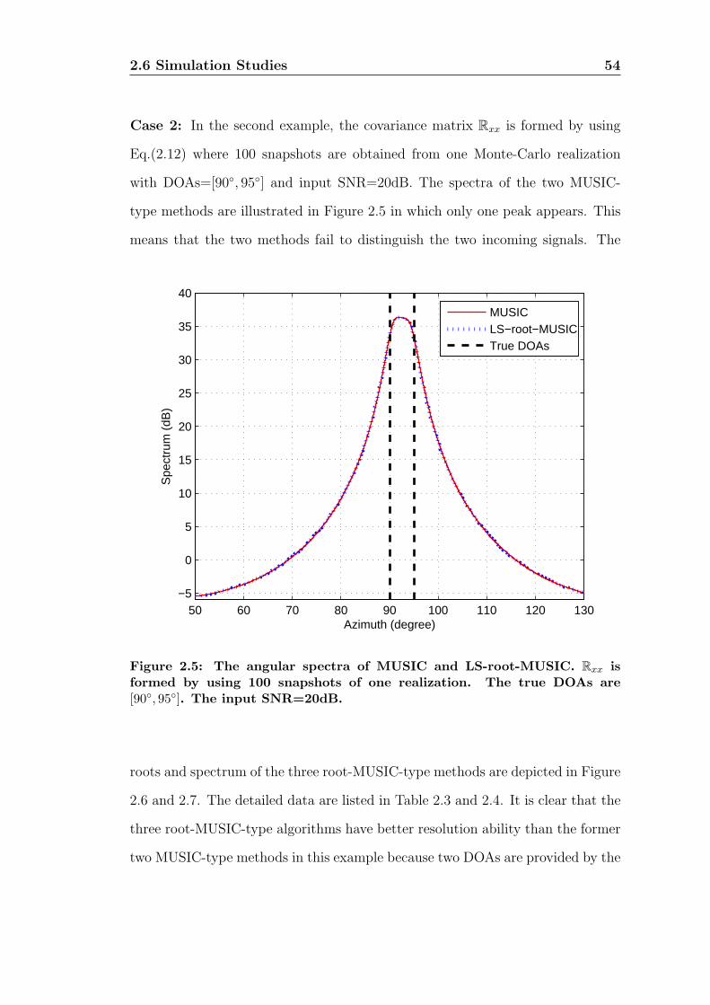
Case 2: In the second example, the covariance matrix Rxx is formed by using
Eq.(2.12) where 100 snapshots are obtained from one Monte-Carlo realization
with DOAs=[90, 95] and input SNR=20dB. The spectra of the two MUSIC-
type methods are illustrated in Figure 2.5 in which only one peak appears. This
means that the two methods fail to distinguish the two incoming signals. The
50 60 70 80 90 100 110 120 130−5
0
5
10
15
20
25
30
35
40
Azimuth (degree)
Spe
ctru
m (
dB)
MUSICLS−root−MUSICTrue DOAs
Figure 2.5: The angular spectra of MUSIC and LS-root-MUSIC. Rxx isformed by using 100 snapshots of one realization. The true DOAs are[90, 95]. The input SNR=20dB.
roots and spectrum of the three root-MUSIC-type methods are depicted in Figure
2.6 and 2.7. The detailed data are listed in Table 2.3 and 2.4. It is clear that the
three root-MUSIC-type algorithms have better resolution ability than the former
two MUSIC-type methods in this example because two DOAs are provided by the

2.6 Simulation Studies 55
latter three methods, which can be explained by the fact that the root-MUSIC-
type methods are insensitive to the radial errors [17]. Also, it can be found
in Table 2.3 and 2.4 that the three root-MUSIC-type approaches yield the same
roots of interest. One important observation is that the radii corresponding to the
true DOAs are not exactly equal to unit anymore. This is due to the perturbation
caused by the covariance matrix estimation using finite snapshots. In practice,
the perturbation is unavoidable. Therefore it is more sensible to find the DOAs
on the circles with radius rather than unit.
0 50 100 150 200 250 300 350
0.6
0.8
1
1.2
1.4
1.6
1.8
Azimuth (degree)
Mag
nitu
de (
dB)
extended root−MUSICProposed iterative method
Figure 2.6: Roots for the extended root-MUSIC and the proposed iterativefast root-MUSIC. Rxx is formed by using 100 snapshots of one realization.The true DOAs are [90, 95]. The input SNR=20dB.
2.6 Simulation Studies 56
Azimuth (degree)
Azimuth (degree)
Radiu
sr
Radiu
sr
Spectr
um
(dB
)
Figure 2.7: The 2-D spectrum of the proposed IDFT-based method (and
contour diagram), where ρ ∈ [0.5, 1] and ∆ρ = 0.01. Rxx is formed by using
100 snapshots of one realization. The true DOAs are [90, 95]. The input
SNR=20dB.

2.6 Simulation Studies 57
Table 2.3: The roots of the extended root-MUSIC and the proposed iter-ative fast root-MUSIC when the covariance matrix Rxx is formed by using100 snapshots of one realization.
extended root-MUSIC proposed iterative fast root-MUSIC
1.5987− 0.8297i = 1.80e−j27.43π/180
−1.2747 + 0.9778i = 1.61e−j217.49π/180
0.8488 + 1.1989i = 1.47e−j305.30π/180
−0.1479 + 1.4246i = 1.43e−j264.07π/180
−0.0784− 1.0296i = 1.03e−j94.35π/180
−0.0136− 1.0305i = 1.03e−j90.75π/180
−0.0128− 0.9702i = 0.97e−j90.75π/180 −0.0128− 0.9702i = 0.97e−j90.75π/180
−0.0735− 0.9657i = 0.97e−j94.35π/180 −0.0735− 0.9657i = 0.97e−j94.35π/180
−0.0721 + 0.6945i = 0.70e−j264.07π/180
0.3934 + 0.5556i = 0.68e−j305.30π/180
−0.4939 + 0.3788i = 0.62e−j217.49π/180
0.4928− 0.2557i = 0.56e−j27.43π/180
Table 2.4: (ρ, θ) pairs of the peaks of LS-root-MUSIC and the proposedIDFT-based method when the covariance matrix Rxx is formed by using 100snapshots of one realization.
LS-root-MUSIC proposed IDFT-based method(1.00, 91.76) (0.97, 90.70)
(0.97, 94.31)(0.70, 264.02)(0.68, 305.24)(0.62, 217.44)(0.56, 27.38)
In the following three examples, the root-mean-square-error (RMSE) per-
formance of DOA estimation is concerned. For each scenario, the average of 500
independent Monte-Carlo runs is used to obtain each simulated point.
Case 3: In the third example, the DOA of the second signal source varies from 91
to 100 whereas the DOA of the first signal is fixed at 90. All other parameters
are chosen as the same as that in the second example. In Figure 2.8, the DOA
estimation RMSEs versus the signal angular separation are presented.
2.6 Simulation Studies 58
1 2 3 4 5 6 7 8 9 1010
−1
100
101
102
θ2−θ
1 (degrees)
RM
SE
(de
gree
s)
MUSICL−S root−MUSICextended root−MUSICproposed iterative methodproposed IDFT−based method
Figure 2.8: DOA estimation RMSEs versus (θ2−θ1) with the snapshot num-
ber = 100, input SNR=20dB, θ1 = 90, ρ ∈ [0.9, 1] and ∆ρ = 0.01.
Case 4: In the fourth example, the performances with different numbers of
snapshots are investigated while all other parameters remain as in the second
example. The DOA estimation RMSEs versus the snapshot number are displayed
in Figure 2.9.

2.6 Simulation Studies 59
101
102
103
10−1
100
101
102
The number of snapshots
RM
SE
(de
gree
s)
MUSICL−S root−MUSICextended root−MUSICproposed iterative methodproposed IDFT−based method
Figure 2.9: DOA estimation RMSEs versus the snapshot number with input
SNR=20dB, DOAs=[90, 95], ρ ∈ [0.9, 1] and ∆ρ = 0.01.
Case 5: The last example studies the impact of input SNR on the five methods
tested. Also, all other parameters are the same as in the second example. The
DOA estimation RMSEs versus input SNR are plotted in Figure 2.10.
All the three figures demonstrate that the proposed two algorithms pro-
vide the asymptotically similar performance in DOA estimation to the extended
root-MUSIC. Furthermore, as expected, the proposed algorithms have superior
capability to MUSIC-type methods in the situations: when two signal sources are
closely spaced, when the snapshot number is quite small, or when input SNR is
low.

2.7 Summary 60
5 10 15 20 25 3010
−1
100
101
102
103
Input SNR (dB)
RM
SE
(de
gree
s)
MUSICL−S root−MUSICextended root−MUSICproposed iterative methodproposed IDFT−based method
Figure 2.10: DOA estimation RMSEs versus the input SNR with
DOAs=[90, 95], the snapshot number =100, ρ ∈ [0.9, 1] and ∆ρ = 0.01.
2.7 Summary
Two computationally efficient root-MUSIC algorithms for arbitrary arrays have
been presented in this chapter. The extended root-MUSIC has made it possi-
ble to apply the traditional root-MUSIC to the arrays with arbitrary geometry.
However, the problem that the extended root-MUSIC has to face is that a poly-
nomial with very high order is required to root, which may be computationally
expensive.

2.7 Summary 61
Considering the facts that the roots appear in conjugate reciprocal pairs
and the roots of interest are closest to the unit circle, the first proposed iterative
method suggests a framework in which, rather than computing all roots, only the
wanted roots need to be computed. It basically consists of a combination of the
spectral factorization and large eigenvalue finding. The polynomial is efficiently
split, via the Schur algorithm, into two factors with roots, respectively, inside
and outside the unit circle. The Schur algorithm exploits the Toeplitz structure
to complete triangular factorization. The desired roots are corresponding to a
few large roots of the new polynomial with roots inside the unit circle. Then
Arnoldi iteration is utilized to compute only the large eigenvalues of the associated
companion matrix.
The second proposed method is an IDFT-based root-MUSIC in which the
DOAs are obtained by scanning a range of circles. The essence behind is that due
to the inevitable perturbation the roots corresponding to the true DOAs are no
longer located on the unit circle and hence multiple circles need to be concerned.
The second proposed algorithm is computationally efficient as IDFT is adopted
and it is readily to scan all circles in parallel.
The analysis and simulation results verify that the proposed algorithms,
with less computational burden, have the asymptotically similar performance in
DOA estimation to the extended root-MUSIC. Also, the proposed algorithms have
superior resolution ability to LS-root-MUSIC (which is a MUSIC type algorithm)
and the conventional MUSIC, particularly when two signal sources are located
close to each other in space, the number of snapshots is relatively small, or the
input SNR is low.
2.8 Appendix 2.A Arnoldi Iteration 62
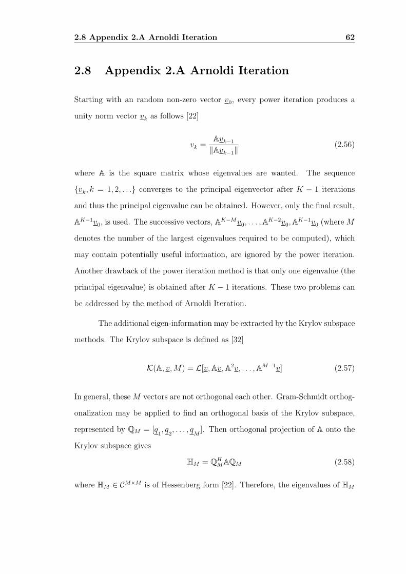
2.8 Appendix 2.A Arnoldi Iteration
Starting with an random non-zero vector v0, every power iteration produces a
unity norm vector vk as follows [22]
vk =Avk−1
∥Avk−1∥(2.56)
where A is the square matrix whose eigenvalues are wanted. The sequence
vk, k = 1, 2, . . . converges to the principal eigenvector after K − 1 iterations
and thus the principal eigenvalue can be obtained. However, only the final result,
AK−1v0, is used. The successive vectors, AK−Mv0, . . . ,AK−2v0,AK−1v0 (whereM
denotes the number of the largest eigenvalues required to be computed), which
may contain potentially useful information, are ignored by the power iteration.
Another drawback of the power iteration method is that only one eigenvalue (the
principal eigenvalue) is obtained after K − 1 iterations. These two problems can
be addressed by the method of Arnoldi Iteration.
The additional eigen-information may be extracted by the Krylov subspace
methods. The Krylov subspace is defined as [32]
K(A, v,M) = L[v,Av,A2v, . . . ,AM−1v] (2.57)
In general, theseM vectors are not orthogonal each other. Gram-Schmidt orthog-
onalization may be applied to find an orthogonal basis of the Krylov subspace,
represented by QM = [q1, q
2, . . . , q
M]. Then orthogonal projection of A onto the
Krylov subspace gives
HM = QHMAQM (2.58)
where HM ∈ CM×M is of Hessenberg form [22]. Therefore, the eigenvalues of HM

2.8 Appendix 2.A Arnoldi Iteration 63
can be computed efficiently. Also, the M eigenvalues are supposed to converge
to the M largest eigenvalues of A. Here only rudiments of Arnoldi Iteration are
presented. For further details, see [31, 32].
64
Chapter 3
Matched Direction Beamforming
based on Signal Subspace
IN this chapter, the problem of constructing the matched direction beamformer
(MDB) is studied, without using the interference subspace. MDB is referred
to as the beamformer resolving the desired signal that is drawn from an unknown
direction inside a known subspace [40, 41]. Due to many practical reasons, the
exact knowledge of the DOA of the desired signal is often unavailable, which
causes the mismatch between the actual and the nominal manifold vectors. For
instance, the DOA estimator may be lacking in accuracy. In this chapter, the
manifold vector of the desired signal in the presence of pointing errors is assumed
to lie in a known linear subspace, but it remains unknown. The main contribution
of this chapter is to propose a new MDB that can find the manifold associated
with the desired signal without the knowledge of the interference subspace. The
proposed approach is based on searching for the principal eigenvector of a certain
rank-one matrix consisting of the signal subspace and the subspace which the
desired signal belongs to. Furthermore, the proposed MDB is robust to both
pointing errors and the dimension overestimation of the signal subspace.
3.1 Received Signal Model 65
3.1 Received Signal Model
Consider an array with N sensors collects one desired signal and M interference
signals. The (M + 1) signals are assumed to be narrow-band, uncorrelated to
each other and located in the far field. The received signal vector is given by
x(t) = S(θd)md(t) +M∑i=1
S(θi)mi(t) + n(t) (3.1)
where the subscript (·)d stands for the desired signal. θi and mi(t) represent,
respectively, the DOA and complex envelope of the ith interference signal. The
DOA of the desired signal, θd, is often not perfectly known in practical appli-
cations. This “pointing” errors can result in the difference between the actual
manifold and the presumed (nominal) manifold. That is
if θd = θ0, then S(θd) = S(θ0) (3.2)
where θ0 is the presumed DOA used by the array processor.
The straightforward consequence of this mismatch in DOA is to cause a
substantial performance degradation of conventional adaptive beamformers (for
further details, see the next chapter or [8]). As θd is unknown, the corresponding
manifold vector S(θd) remains unknown. However, S(θd) lies in a known p-
dimension (where p > 1 ) linear subspace L[H] and thus can be written as a
linear combination of the bases of L[H] [40, 41]. This means that the manifold
vector S(θd) can be expressed as
S(θd) = Hb (3.3)
where the vector b is referred to as the linear combination vector. Note that b

3.1 Received Signal Model 66
and S(θd) are unknown in practical situation, while H is a known matrix. Next,
two examples will be presented to demonstrate how to obtain the matrix H.
In the first example, the actual manifold is expanded in Taylor series
around the presumed manifold S(θ0) as [40,42,43]
S(θd) = S(θ0 +∆θd) = S(θ0) +∞∑k=1
(∆θd)k
k!
∂kS(θ)
∂θk
∣∣∣∣θ=θ0
(3.4)
with
∆θd = θd − θ0 (3.5)
where the nominal DOA, θ0, is known. In practice the first two order derivatives
are enough to satisfy the wanted precision. For the details of the expressions for
the first two order derivatives, see Appendix 3.A. Hence a matrix can be defined
as
H1 = [S0, S(θ0),S(θ0)] (3.6)
where S(θ0) and S(θ0) denote the first and second derivatives with respect to θ0.
H1 can be computed prior to the beamformer processing if the presumed θ0 and
array geometry information are at hand. Therefore it is reasonable to assume
that H1 can be formed using the nominal direction. In the case when the array
reference point is chosen as the centroid point of the array, the columns of H1 are
orthogonal to each other [2]. Then the manifold of interest may be approximated
as
S(θd) ≈ H1
1
∆θd
(∆θd)2
2
︸ ︷︷ ︸
∆=b1
(3.7)
where b1 is unknown.

3.1 Received Signal Model 67
Alternatively, using the Taylor series expansion and retaining the terms
up to the second order, one has the following approximations
S(θ0) = S(θd −∆θd) (3.8a)
≈ S(θd)−∆θdS(θd) +(∆θd)
2
2S(θd)
S(θ0 ±∆θ) = S(θd ±∆θ −∆θd) (3.8b)
≈ S(θd) + (±∆θ −∆θd)S(θd) +(±∆θ −∆θd)
2
2S(θd)
where ∆θ is related to the expected range of the DOA of the desired signal and
can be a given value even if the true DOA is unavailable. This means that ∆θ is
known. Generally the value of ∆θ is set such that |∆θ ±∆θd| is insignificant so
that the above approximations are valid. Now S(θd) may be rewritten as
S(θd) ≈ (∆θ)2 − (∆θd)2
(∆θ)2S(θ0) +
(∆θd)2 +∆θ∆θd2(∆θ)2
S(θ0 +∆θ)
+(∆θd)
2 −∆θ∆θd2(∆θ)2
S(θ0 −∆θ)
= [S(θ0), S(θ0 +∆θ), S(θ0 −∆θ)]︸ ︷︷ ︸∆=H2
(∆θ)2−(∆θd)
2
(∆θ)2
(∆θd)2+∆θ∆θd
2(∆θ)2
(∆θd)2−∆θ∆θd
2(∆θ)2
︸ ︷︷ ︸
∆=b2
(3.9)
Hence S(θd) also belongs to the known linear subspace L[S(θ0), S(θ0−∆θ), S(θ0+
∆θ)] and the associated linear combination vector b2 is unknown.
In [44–46], an uncertainty model called flat ellipsoidal uncertainty set has
been discussed in which the true manifold vector is expressed as
S(θd) = S(θ0) + Bbfe , ∥bfe∥ ≤ 1 (3.10)

3.1 Received Signal Model 68
where B is a known N × (p− 1) matrix with full column rank, and the vector bfe
is unknown. Clearly the actual manifold can be rewritten as
S(θd) = H[1, bTfe]T (3.11)
where H = [S(θ0),B]. Therefore the flat ellipsoidal uncertainty set can be trans-
formed to the linear subspace model of (3.3).
In this thesis, the unknown vector b is assumed to stay unchanged during
the observation interval of L successive snapshots although it may vary in the next
L snapshots. The contribution of the desired signal to the covariance matrix Rxx
is given by
Rdd = E(md(t)S(θd)) (md(t)S(θd))H
= Emd(t)m∗d(t)S(θd)SH(θd)
= σ2dHb b
HHH (3.12)
which is a rank-1 matrix obviously. Under the assumption that theM interference
signals are uncorrelated with the desired signal, the second-order model for x(t)
can be written as
Rxx = σ2dHb b
HHH + Ri + σ2nI (3.13)
where the rank-M matrix Ri represents the interference effects and may have the
following form
Ri =M∑i=1
σ2i S(θi)S
H(θi) (3.14)
The so-called matched direction beamforming (MDB) is referred to as the
beamformer resolving the signal that are drawn from an unknown direction b
inside the known subspace L[H] [40, 41]. The main task of this chapter is to

3.2 Previous Work 69
design a MDB which is robust to pointing errors.
3.2 Previous Work
Two related existing approaches regarding MDB will be briefly introduced. These
are:
1. MDB with the knowledge of interference subspace
2. Multirank minimum-variance-distionless-response (MVDR) beamformer
3.2.1 MDB with the Knowledge of Interference Subspace
Let SI represent the matrix consisting of the interference manifold vectors. That
is
SI = [S(θ1), . . . , S(θM)] (3.15)
In [40], it assumes that SI is exactly known and the authors derive a maximum-
likelihood estimator of the vector b, given by
b = βP(UHU)−1UHRxxU (3.16)
where the notation P· stands for the principal eigenvector of the matrix argu-
ment between braces, and the matrix U is defined as
U = P⊥SIH (3.17)
with
P⊥SI = I− SI(SH
I SI)−1SH
I (3.18)

3.2 Previous Work 70
The coefficient β is a normalization constant. Note that the array beamformer
output SNIR is independent of β. Finally the weight vector of the MDB is
expressed as
w = βP⊥SIHb = βUb (3.19)
where the coefficient β can be determined such that ∥wHw∥ = 1. The above
beamformer intends to cancel the interferences completely while being matched
to the best direction in the interference-free signal subspace.
The problem in [40] is that the perfect knowledge of the interference sub-
space is required for its implementation. In many practical applications, unfor-
tunately, this assumption is not always valid or the interference subspace cannot
be estimated easily.
3.2.2 Multirank MVDR Beamformer
In [41], a multirank minimum-variance-distionless-response (MVDR) beamformer
is presented. This beamformer may be implemented by using a generalized side-
lobe canceller (GSC) [47], illustrated in Figure 3.1. In the GSC, the input array
signal vector x(t) ∈ CN is firstly decomposed into two parts: HHx(t) ∈ Cp and
QHx(t) ∈ C(N−p). Note that here the columns of H are required to be orthonor-
mal columns, i.e., HHH = Ip. For the general H the Gram-Schmidt algorithm [22]
may be employed to render the columns of H orthonormal. Q ∈ CN×(N−p) is a
left-orthogonal matrix that makes [H Q] unitary, i.e., [H Q][H Q]H = IN .

3.2 Previous Work 71
( )y t
⊗
⊗ ⊗
⊗( )x t
( )e t
Formee
⊗
Vector
Matrix
Scalar
k1N 1×
p 1×
(N -p) 1× p 1×
p 1×
k 1×
Figure 3.1: The GSC structure of the multirank MVDR beamformer
The middle branch of the GSC passes the desired signal and part of inter-
ferences and noise that lie in L[H]. The bottom branch is the sidelobe canceling
path where the desired signal is blocked. Then the residual signal e(t) ∈ Cp is
formed by
e(t) = HHx(t)− FHQHx(t) (3.20)
where FH = HHRxxQ(QHRxxQ)−1 is designed by using the criterion of the linear
minimum mean-squared error (LMMSE) so that the power of e(t) is minimized.
The second-order statistics of e(t) is represented by the matrix Ree
Ree = Ee(t)eH(t)
= HHRxxH−HHRxxQ(QHRxxQ)−1QHRxxH (3.21)
3.2 Previous Work 72
Alternatively, it is shown in [41] that Ree has a simplified form as
Ree =(HHR−1
xxH)−1
(3.22)
Finally, the desired signal is extracted from e(t) by a weight matrix W. The key
idea of the multirank MVDR beamformer is how to design the weight matrix W.
Let us start from the simple case where only one interference is present. Then
the matrix Ree may be expressed as
Ree = σ2db b
H + ηHHS(θ1)SH(θ1)H+ σ2
nI (3.23)
where S(θ1) is the manifold vector of the interference signal. η represents the
level how the interference is suppressed by the GSC beamformer, which is given
by [41]
η =σ21σ
2n
σ2n + σ2
1SH(θ1)P⊥
HS(θ1)(3.24)
It is clear that b may be approximated by the principal eigenvector of Ree up to
a scaling factor if the desired signal subspace L[H] and the interference subspace
L[S(θ1)] are well separated. However, when the interference subspace is relatively
close to L[H], the effects of interferences on Ree cannot be neglected any more.
The immediate consequence is that the principal eigenvector contains significant
contributions from the interference. On the other hand, the desired signal con-
tributes not only to the principal eigenvector but also the other eigenvectors. In
order to deal with this situation, [41] suggests that, instead of one eigenvector,
a set of dominant eigenvectors of Ree (i.e., the eigenvectors corresponding to a
few largest eigenvalues of Ree), say k dominant eigenvectors, should be utilized to
restore the desired signal. This is the so-called multirank MVDR beamforming.
Thus the weight matrix of the multirank MVDR for the general case may
3.3 Proposed Matched Direction Beamformer 73
be explicitly expressed as
W = R−1xxHReeJ (3.25)
where J is composed of k dominant eigenvectors of Ree. In addition, the inequa-
tions k 6M +1 6 p must hold for the multirank MVDR. Finally, these multiple
outputs are summed up by multiplication with the k× 1 unit vector 1k to obtain
the final output. The array output SNIR can be written as
SNIRout =trWHRddW
trWH(Ri + σ2nI)W
(3.26)
The major drawbacks associated with the multirank MVDR beamformer are:
1. each column of W is contaminated by the interferences, particularly when
the interferences are close to the desired signal, which results in the degra-
dation of array output SNIR;
2. the signal number is required to be not greater than the dimension of H,
i.e., M + 1 ≤ q; hence this method fails in the case where a large number
of interferences are present;
3. it is not clear how many dominant eigenvectors (i.e., the value of k) should
be selected to build J.
3.3 Proposed Matched Direction Beamformer
3.3.1 Estimate using Signal Subspace
Performing eigen-decomposition on Rxx yields:
Rxx =N∑i=1
λiEiEHi (3.27)

3.3 Proposed Matched Direction Beamformer 74
where the eigenvalues λi, i = 1, . . . , N are the eigenvalues arranged in decreas-
ing order (i.e., λ1 ≥ . . . ≥ λN). Ei is the eigenvector associated with λi.
Inspired by [40], here an algorithm is developed, which is able to esti-
mate the linear combination vector b without the knowledge of the interference
subspace. The key point of this algorithm is supported by the following lemma.
Lemma 3.1: The vector b is the principal eigenvector of a rank-1 matrix Zℓ
up to a scaling factor, where the matrix Zℓ is defined as
Zℓ = (UHℓ Uℓ)
−1UHℓ EℓE
Hℓ Uℓ (3.28)
with
Uℓ = P⊥AℓH (3.29)
The matrix Aℓ is composed of all the M + 1 signal eigenvectors except Eℓ, i.e.,
Aℓ = [E1, . . . , Eℓ−1, Eℓ+1, . . . , EM+1] (3.30)
Eℓ can be any M + 1 signal eigenvector.
Proof: Eℓ can be written as:
Eℓ = Eℓ(EHℓ Eℓ)
−1EHℓ S(θd)
EHℓ S(θd)
=Eℓ(E
Hℓ Eℓ)
−1EHℓ S(θd)
EHℓ S(θd)
=PEℓ
S(θd)
EHℓ S(θd)
(3.31)
where the fact (EHℓ Eℓ)
−1 = 1 is used in the above. Eℓ lies in the signal-subspace,
implying that Eℓ is the combinations of the manifolds of the desired signal and
all interferences. Hence EHℓ S(θd) = 0 holds. Inserting (3.31) into Zℓ defined in
3.3 Proposed Matched Direction Beamformer 75
(3.28) yields
Zℓ =1
EHℓ S(θd)
(UHℓ Uℓ)
−1UHℓ PEℓ
S(θd)︸ ︷︷ ︸∆=ζ
EHℓ Uℓ (3.32)
Let Pn denote the projection onto the noise subspace L[EM+2, . . . , EN ]. Then
one has the followings
PnS(θd) = 0
PEℓ+ PAℓ
+ Pn = I (3.33)
Consequently, the term ζ can be rewritten as
ζ = UHℓ (I− PAℓ
− Pn)S(θd)
= UHℓ S(θd)− UH
ℓ PAℓS(θd)− UH
ℓ PnS(θd)︸ ︷︷ ︸=0
= UHℓ S(θd)−HHP⊥
AℓPAℓ︸ ︷︷ ︸
=O
S(θd)
= UHℓ S(θd) (3.34)
where the Hermitian property of projection operator P⊥Aℓ
= (P⊥Aℓ)H is used. Re-
placing the term ζ in (3.32) by (3.34) gives
Zℓ =1
EHℓ S(θd)
(UHℓ Uℓ)
−1UHℓ S(θd)E
Hℓ Uℓ
=1
EHℓ S(θd)
(UHℓ Uℓ)
−1HHP⊥AℓHb EH
ℓ Uℓ
=1
EHℓ S(θd)
(UHℓ Uℓ)
−1HHP⊥AℓP⊥AℓHb EH
ℓ Uℓ
=1
EHℓ S(θd)
(UHℓ Uℓ)
−1UHℓ Uℓb E
Hℓ Uℓ
=1
EHℓ S(θd)
b EHℓ Uℓ (3.35)
where the idempotent property of projection operator P⊥Aℓ
= P⊥AℓP⊥Aℓ, the Hermi-

3.3 Proposed Matched Direction Beamformer 76
tian property of projection operator P⊥Aℓ
= (P⊥Aℓ)H , and the modelling S(θd) = Hb
(see Eq.(3.3)) are utilized. Finally multiplying both sides of (3.35) by b produces
Zℓb =
(EH
ℓ Uℓb
EHℓ S(θd)
)︸ ︷︷ ︸
scalar
b (3.36)
It is obvious that the vector b is the principal eigenvector of the rank-1 matrix
Zℓ up to a scaling factor.
In practice, the covariance matrix Rxx is estimated by Eq.(2.12). If the
number of snapshots acquired by the array is quite small, the orthogonality be-
tween Pn and S(θd) may be impaired due to the effect of finite snapshot, partic-
ularly when the magnitudes of eigenvalues corresponding to the noise subspace
are small. In such case, the term ζ becomes ζ = UHℓ S(θd) − UH
ℓ PnS(θd). Thus
the estimated principal eigenvector and the corresponding manifold become
b(ℓ)
= βb− β(UH
ℓ Uℓ
)−1 UHℓ PnS(θd)
S(ℓ)(θd) = Hb
(ℓ)= βS(θd)− βH
(UH
ℓ Uℓ
)−1 UHℓ PnS(θd) (3.37)
where β is determined such that ∥S(ℓ)(θd)∥2 = N . With the increasing of snapshot
number, PnS(θd) and the estimation error both tend to zero. Keeping in mind
that the estimates in (3.37) are obtained from the matrix Zℓ where the ℓth signal-
subspace eigenvector is excluded from Aℓ, one can find (M + 1) estimates of b if
Zℓ, ℓ = 1, 2, . . . ,M+1 are used. For the purpose of estimation error reduction,
the proposed method employs the average of these (M + 1) estimates instead of
3.3 Proposed Matched Direction Beamformer 77
one estimate, i.e.,
b =1
M + 1
M+1∑ℓ=1
b(ℓ)
S(θd) = Hb = H
(1
M + 1
M+1∑ℓ=1
b(ℓ)
)(3.38)
The weight vector of the proposed MDB can be constructed as
wprop = R−1xxHb =
R−1xxH
M + 1
M+1∑ℓ=1
b(ℓ)
(3.39)
In summary, the proposed MDB algorithm consists of the following steps.
1. Estimate the covariance matrix Rxx by using the received snapshots and
perform eigen-decomposition on Rxx to obtainM+1 signal-subspace eigen-
vectors Ei, i = 1, · · · ,M + 1.
2. For ℓ = 1, · · · ,M + 1, form the matrix Zℓ in (3.28) and compute the asso-
ciated principal eigenvector to obtain the vector b(ℓ).
3. Average theseM+1 vectors b(ℓ), ℓ = 1, · · · ,M+1 to obtain b (see (3.38)).
4. Use (3.39) to compute the weight vector of the proposed MDB beamformer.
3.3.2 Some Discussions
The assumption made in Lemma 3.1 is that signal subspace eigenvectors
[E1, . . . , EM+1] are available, which is a quite weak assumption compared with the
assumption in [40] where it assumes the interference subspace, L[SI ], is perfectly
known.
Consider the case when the signal subspace dimension M + 1 is overes-
3.4 Simulation Studies 78
timated. Then the dimensionality of the noise subspace is reduced. However,
the projector Pn with reduced dimensionality is still orthogonal to S(θd), which
implies that Lemma 3.1 is valid in this case as well. Therefore the proposed
method is robust to the overestimation of signal subspace. If the signal subspace
dimension is underestimated, the estimated noise subspace would contain signal
component which renders Pn not orthogonal with S(θd) any more. Thus the
proposed method fails in the case of dimension underestimation.
In [41, 48], the situation where the vector b is not constant but random
during the L snapshot observation time due to the fast varying environment has
been considered. In this case, the contribution due to the desired signal is given
by
Rdd = σ2dHRbbH (3.40)
where Rbb = Eb bH is a full rank matrix (rank-p). Therefore, Rdd becomes a
rank-p matrix. In [41] only the simplest case where the rank-p matrix Rbb is
assumed to be known is studied. Using Corollary VI.2 of [48] one can estimate
the rank-p matrix associated with the desired signal even if the structure of the
rank-p matrix is unknown. However, this approach cannot be employed in the
scenario of this thesis. This is because that when using Corollary VI.2 of [48],
Rbb is required to be full rank such that its inversion, R−1bb , exists. Nevertheless,
in the situation of this thesis the matrix Rbb = b bH is of rank-one and hereby
non-invertible.
3.4 Simulation Studies
In order to evaluate the effectiveness of the proposed MDB, a number of simula-
tion studies have been carried out using, without any loss of generality, a uniform
3.4 Simulation Studies 79
linear array with N = 10 sensors and half-wavelength sensor spacing. Note that
the proposed method is applicable to arrays with arbitrary geometries. The array
operates in the presence of three equally powered source signals where one is the
desired signal and two are interferences. It is assumed a 3 pointing error in the
desired signal direction with the actual DOA θd = 90 and the nominal DOA
θ0 = 87. The matrix H is obtained by using Eq.(3.6).
Case 1: In the first example, the powers of three signals are all unit and the
noise power is σ2n = 0.1. The first interference signal is fixed at 100 while the
DOA of the second interference varies from 67 to 86. The covariance matrix Rxx
has the theoretical form as Eq.(3.13). Four methods below have been simulated:
1. the multirank MVDR
2. the traditional Wiener-Hopf
3. the MDB proposed in [40] (see Eq.(3.19)) where the perfect knowledge of
the interference subspace (IS) is assumed to be known
4. the proposed method
The weight vector of the Wiener-Hopf processor is given by [5]
wWH = R−1xxS(θ0) (3.41)
The SNIR performances of these methods versus the DOA of the second
interference are displayed in Figure 3.2 where the legend ‘Multirank MVDR-k’
means that k dominant eigenvectors of Ree are used to form the weight matrix in
Eq.(3.25).

3.4 Simulation Studies 80
68 70 72 74 76 78 80 82 84 860
2
4
6
8
10
12
14
16
18
20
Azimuth of the 2nd Interference (degrees)
Arr
ay O
utpu
t SN
IR (
dB)
Multrank MVDR−1Multrank MVDR−2Multirank MVDR−3Wiener−HopfProposed MDBMDB with known IS
Figure 3.2: Array output SNIR versus the azimuth of the 2nd interference.
The 1st interference remains at 100. The actual DOA of the desired signal
is 90 while the presumed DOA is 87.
It can be seen from Figure 3.2 that the multirank MVDR with only the
principal eigenvector of Ree is better than that with two or three dominant eigen-
vectors. That is because the second and third dominant eigenvectors contain
significant effects of the interferences. When the second interference is far away
from the the desired signal (the DOA of the second interference is less than 79
in this example), MDB with perfect knowledge of the interference subspace, the
multirank MVDR-1 and the proposed MDB have similar performance. Compared
with the multirank MVDR, Figure 3.2 shows that the second interference has to
be closer to the direction of the desired signal before it leads to a SNIR deteri-
oration for the proposed method. The superiority of the MDB in [40] over the
proposed method is mainly due to the assumption used in [40] that the exact

3.4 Simulation Studies 81
knowledge of the interference subspace is available at all times. Note that this
assumption, however, is often impractical in many situations. The SNIR of the
proposed algorithm begins to degrade when the DOA of the second interference
is greater than 81. That is because the second interference, as well as the de-
sired signal, lies in the subspace L[H] if the DOA of the second interference is
very close to the nominal DOA. Figure 3.2 also illustrates that the conventional
Wiener-Hopf is quite susceptible to the pointing errors in this example.
Case 2: All the parameters in the second example are the same as that in the
first example, except that the DOA of the first interference moves closer to the
desired signal (which changes from 100 to 97). Figure 3.3 indicates that there
exists a big gap between the multirank MVDR and the proposed method as well
as the MDB in [40] even when the second interference is far away from the desired
signal. This is because the first interference and the desired signal are closer in
space than the first example, and thus the principal eigenvector of Ree contains
significant component of the first interference. However, the proposed method
maintains its performance.
Case 3: In this example, the scenario is identical to the first example, but the
DOA of the second interference is fixed at 80 and the input SNR varies between
-10dB and 10dB. Figure 3.4 demonstrates that proposed method achieves the
similar array output SNIR performance as that of the MDB using the exact
knowledge of interference subspace. Also, as depicted in Figure 3.4, the multirank
MVDR fails when input SNR is lower than -2dB because the noise dominates the
principal eigenvector of Ree if the noise power is too strong.

3.4 Simulation Studies 82
68 70 72 74 76 78 80 82 84 860
2
4
6
8
10
12
14
16
18
20
Azimuth of the 2nd Interference (degrees)
Arr
ay O
utpu
t SN
IR (
dB)
Multrank MVDR−1Multrank MVDR−2Multirank MVDR−3Wiener−HopfProposed MDBMDB with known IS
Figure 3.3: Array output SNIR versus the azimuth of the 2nd interference.The 1st interference remains at 97. The actual DOA of the desired signalis 90 while the presumed DOA is 87.
−10 −5 0 5 100
2
4
6
8
10
12
14
16
18
20
Input SNR (dB)
Arr
ay O
utpu
t SN
IR (
dB)
Multrank MVDR−1Multrank MVDR−2Multirank MVDR−3Proposed MDBMDB with known IS
Figure 3.4: Array output SNIR versus the input SNR. The two interference
DOAs are at [80, 100]. The actual DOA of the desired signal is 90 while
the presumed DOA is 87. All signals are equally powered.

3.4 Simulation Studies 83
Case 4: The robustness of the proposed algorithm to the overestimation or
underestimation of the signal subspace dimension is examined in the fourth ex-
ample, with the same simulation scenario as the first example except that the
second interference is fixed at 80. The nominal signal subspace dimension is
changed from 1 to 9, while the actual dimension is always 3 (i.e., M + 1 = 3).
Figure 3.5 illustrates that the SNIR performance of the proposed method main-
tains when the nominal dimension is between 3 and 8. The proposed approach
fails when the nominal dimension is underestimated (the nominal dimension is
1 or 2) because the estimated Pn contains the signal component which leads to
PnS(θd) = 0. When the nominal dimension is above 8, the proposed approach
also fails which can be explained by the following fact. If the rank of the matrix
Aℓ in Eq.(3.30) is over 8, then the rank of P⊥Aℓ
is N − 8 = 2. Thus the rank of
the matrix product Uℓ = P⊥AℓH is not greater than 2. Therefore the 3× 3 matrix
UHℓ Uℓ becomes rank deficient and non-invertible.
Case 5: The effect of finite snapshots is investigated in this example, where the
covariance matrix Rxx is estimated by using Eq.(2.12). All other parameters are
the same as the previous example but with the correct signal subspace dimension.
The average of 500 independent simulation runs is used to plot each simulation
point in Figure 3.6. Also, Figure 3.6 indicates that the proposed method is better
than the multirank MVDR.

3.4 Simulation Studies 84
1 2 3 4 5 6 7 8 90
5
10
15
20
The Nominal Signal Subspace Dimension
A
rra
y O
utp
ut
SN
IR (
dB
)
Figure 3.5: Array output SNIR versus the nominal signal subspace dimen-
sion. The true dimension is 3. The actual DOA of the desired signal is 90
while the presumed DOA is 87. The DOAs of interferences are [80, 100].
0 500 1000 1500 2000 25000
2
4
6
8
10
12
14
16
18
20
The Number of Snapshots
Arr
ay O
utpu
t SN
IR (
dB)
Multrank MVDR−1Multrank MVDR−2Multirank MVDR−3Proposed MDBMDB with known IS
Figure 3.6: Array output SNIR versus the snapshot number. The actual
DOA of the desired signal is 90 while the presumed DOA is 87. The DOAs
of interferences are [80, 100].
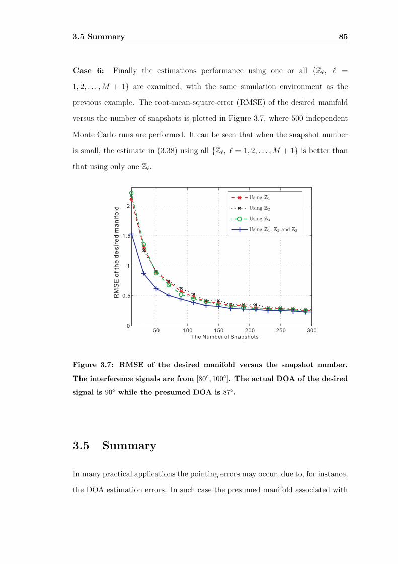
3.5 Summary 85
Case 6: Finally the estimations performance using one or all Zℓ, ℓ =
1, 2, . . . ,M + 1 are examined, with the same simulation environment as the
previous example. The root-mean-square-error (RMSE) of the desired manifold
versus the number of snapshots is plotted in Figure 3.7, where 500 independent
Monte Carlo runs are performed. It can be seen that when the snapshot number
is small, the estimate in (3.38) using all Zℓ, ℓ = 1, 2, . . . ,M + 1 is better than
that using only one Zℓ.
50 100 150 200 250 3000
0.5
1
1.5
2
The Number of Snapshots
RM
SE
of
the
de
sir
ed
ma
nif
old
Using 1
Using 2
Using 3
Using 1, 2 and 3
Figure 3.7: RMSE of the desired manifold versus the snapshot number.
The interference signals are from [80, 100]. The actual DOA of the desired
signal is 90 while the presumed DOA is 87.
3.5 Summary
In many practical applications the pointing errors may occur, due to, for instance,
the DOA estimation errors. In such case the presumed manifold associated with
3.5 Summary 86
the desired signal used by the array system is different than the actual one. The
consequence of this discrepancy is the substantial performance degradation for
the conventional adaptive array beamformers (e.g., the traditional Wiener-Hopf
beamformer), which can be seen in the first and second simulation examples.
In this chapter, the unknown actual manifold vector is modelled as a vec-
tor lying in a known subspace. Two different expressions of this subspace are
also discussed, in which the Taylor series expansion is employed. Thus the true
manifold can be approximated by a product of a known matrix and an unknown
vector. This vector is also called linear combination vector by means of which
the actual manifold can be obtained by linearly combining the subspace bases.
The main contribution of this chapter is that a novel algorithm is devel-
oped to estimate the linear combination vector without the knowledge of the
interference subspace. This means that the condition with the perfect knowledge
of interference subspace in [40] may be relaxed. Instead, the proposed estima-
tor takes use of the signal subspace which can be easily obtained by performing
eigen-decomposition on the covariance matrix. Then a Wiener-Hopf type MDB is
proposed. The theoretical analysis and simulations have proven that the proposed
method is robust to both pointing errors and the dimension overestimation of the
signal subspace. Simulations also reveal that the performance of the proposed
MDB outperforms the multirank MVDR in the case where the interferences are
relatively close to the desired signal or the noise power is quite strong.

3.6 Appendix 3.A The first two derivatives of the manifold vector 87
3.6 Appendix 3.A The first two derivatives of
the manifold vector
This appendix presents the expression of first two derivatives of the manifold
vector with respect to azimuth. The manifold vector may be expressed as follows
S(θ) = exp[−jπ(rx cos θ + ry sin θ)] (3.42)
The first derivative is readily obtained as
S(θ) =∂S(θ)
∂θ(3.43)
= diag(jπ(rx sin θ − ry cos θ))S(θ)
= jπ(rx sin θ − ry cos θ)⊙ S(θ)
where ⊙ denotes the operation of Hadamard product (or elementwise product).
The second derivative is written as
S(θ) =∂2S(θ)
∂θ2(3.44)
= diag(jπ(rx cos θ + ry sin θ))S(θ) +(diag(jπ(rx sin θ − ry cos θ))
)2S(θ)
= jπ((rx cos θ + ry sin θ) + jπ(rx sin θ − ry cos θ)⊙ (rx sin θ − ry cos θ)
)⊙ S(θ)

88
Chapter 4
Interference Cancellation
Beamforming Robust to Pointing
Errors
AN important topic concerned in array signal processing and wireless com-
munications is interference (jammers) rejection. This can be achieved us-
ing a beamformer which places relatively high gain in the direction of the desired
signal and nulls in the directions of the interferences.
The Wiener-Hopf processor suffers from the power inversion problem and
has substantial performance degradation in the presence of pointing errors [8].
By removing the effects of the desired signal, the “modified” Wiener-Hopf avoids
these two problems [49] but allows the interferences to pass through as well.
In this chapter, a novel array processor is presented which not only pre-
vents power inversion and reduces the effect of pointing error but also provides,
asymptotically, complete interference rejection. To eliminate much of the point-
ing error effects, the vector space projections (VSP) method is utilized to find a
new manifold vector. The power of the desired signal can be estimated in one
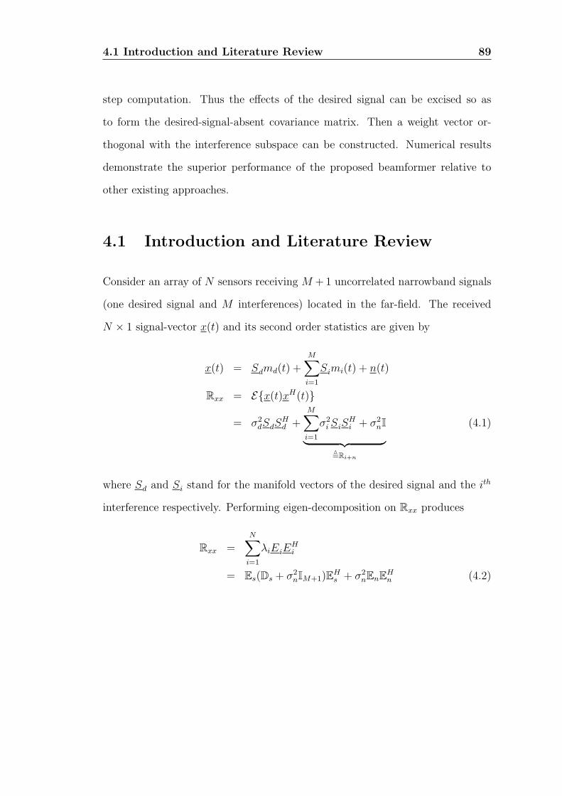
4.1 Introduction and Literature Review 89
step computation. Thus the effects of the desired signal can be excised so as
to form the desired-signal-absent covariance matrix. Then a weight vector or-
thogonal with the interference subspace can be constructed. Numerical results
demonstrate the superior performance of the proposed beamformer relative to
other existing approaches.
4.1 Introduction and Literature Review
Consider an array of N sensors receiving M +1 uncorrelated narrowband signals
(one desired signal and M interferences) located in the far-field. The received
N × 1 signal-vector x(t) and its second order statistics are given by
x(t) = Sdmd(t) +M∑i=1
Simi(t) + n(t)
Rxx = Ex(t)xH(t)
= σ2dSdS
Hd +
M∑i=1
σ2i SiS
Hi + σ2
nI︸ ︷︷ ︸=Ri+n
(4.1)
where Sd and Si stand for the manifold vectors of the desired signal and the ith
interference respectively. Performing eigen-decomposition on Rxx produces
Rxx =N∑i=1
λiEiEHi
= Es(Ds + σ2nIM+1)EH
s + σ2nEnEH
n (4.2)

4.1 Introduction and Literature Review 90
where the eigenvalues λi, i = 1, . . . , N are arranged in decreasing order, the
(M + 1)× (M + 1) diagonal matrix Ds is given by
Ds =
λ1 − σ2n, 0, · · · , 0
0, λ2 − σ2n, · · · , 0
......
. . ....
0, 0, · · · , λM+1 − σ2n
(4.3)
Es and En contain, respectively, the M + 1 dominant eigenvectors and the re-
maining eigenvectors, i.e.,
Es = [E1, · · · , EM+1]
En = [EM+2, · · · , EN ] (4.4)
Therefore the complex N -dimensional observation space H of the data covariance
matrix Rxx can be decomposed into two subspaces: the signal subspace Hs, with
dim [Hs] =M+1, and the noise subspaceHn with dim [Hn] = N−M−1, as shown
in Figure 4.1. The signal subspace Hs is spanned by either the manifold vectors
[Sd, S1, S2, . . . , SM ] or the M +1 dominant eigenvectors [E1, E2, . . . , EM+1], and
the noise subspace Hn by the eigenvectors [EM+2, . . . , EN ]. Also, it is demon-
strated in Figure 4.1 that the interference subspace L[S1, S2, . . . , SM ] is not equal
to the subspace L[E1, E2, . . . , EM ] in the presence of the desired signal.
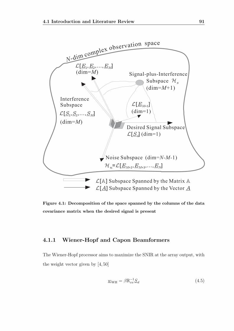
4.1 Introduction and Literature Review 91
H Ln= [ , ..., ]E
M+2E E
M N+3,
L[ ] (dim=1)Sd
L[ ]EM+1
L[ , ..., ]E1E E
2,
M
(dim= )M
(dim= )M
L[ , ..., ]S1S S
2,
M
Hs
(dim= +1)M
Subspace
Signal-plus-Interference
InterferenceSubspace
Desired Signal Subspace
Noise Subspace (dim= 1)N-M-
L[ ] Subspace Spanned by the Matrix
L[ ]A Subspace Spanned by the Vector A
-dim complex
N
observation space
(dim=1)
Figure 4.1: Decomposition of the space spanned by the columns of the data
covariance matrix when the desired signal is present
4.1.1 Wiener-Hopf and Capon Beamformers
The Wiener-Hopf processor aims to maximize the SNIR at the array output, with
the weight vector given by [4, 50]
wWH = βR−1xxSd (4.5)
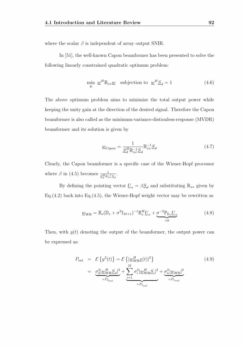
4.1 Introduction and Literature Review 92
where the scalar β is independent of array output SNIR.
In [51], the well-known Capon beamformer has been presented to solve the
following linearly constrained quadratic optimum problem:
minw
wHRxxw subjection to wHSd = 1 (4.6)
The above optimum problem aims to minimize the total output power while
keeping the unity gain at the direction of the desired signal. Therefore the Capon
beamformer is also called as the minimum-variance-distionless-response (MVDR)
beamformer and its solution is given by
wCapon =1
SHd R−1
xxSd
R−1xxSd (4.7)
Clearly, the Capon beamformer is a specific case of the Wiener-Hopf processor
where β in (4.5) becomes 1SHd R−1
xx Sd.
By defining the pointing vector U s = βSd and substituting Rxx given by
Eq.(4.2) back into Eq.(4.5), the Wiener-Hopf weight vector may be rewritten as
wWH = Es(Ds + σ2IM+1)−1EH
s U s + σ−2PEnU s︸ ︷︷ ︸=0
(4.8)
Then, with y(t) denoting the output of the beamformer, the output power can
be expressed as:
Pout = Ey2(t)
= E
|wH
WHx(t)|2
(4.9)
= σ2d|wH
WHSd|2︸ ︷︷ ︸=Pdout
+M∑i=1
σ2i |wH
WHSi|2︸ ︷︷ ︸=PIout
+ σ2n|wWH|2︸ ︷︷ ︸=Pnout

4.1 Introduction and Literature Review 93
where
Pdout = σ2d|UH
s Es (Ds + σ2nIM+1)
−1 EHs Sd|2
PIout =M∑i=1
σ2i |UH
s Es (Ds + σ2nIM+1)
−1 EHs Si|2
Pnout = σ2nU
Hs Es (Ds + σ2
nIM+1)−2 EH
s U s + σ−2n UH
s PEnU s︸ ︷︷ ︸=0
(4.10)
In the absence of any interference signals, PIout = 0 and both Ds and IM+1 become
scalars and equal to Nσ2d and 1 respectively. That is,
Pdout = σ2d|UH
s PEsSd|2
(Nσ2d+σ2
n)2 = σ2
d|UH
s Sd|2
(Nσ2d+σ2
n)2
PIout = 0
Pnout = σ2n
UHs PEsUs
(Nσ2d+σ2
n)2 = σ2
nUH
s Us
(Nσ2d+σ2
n)2
(4.11)
where the fact that PEsSd = Sd is used. From Eq.(4.11) it is clear that desired
output power Pdout is degraded with increasing desired signal power σ2d at the
input of the array, which is referred to as the power inversion problem [49]. For
the desired signal with a high power at the array input, the corresponding desired
signal power at the array output may suffer a sharp reduction which makes it
difficult to detect it.
4.1.2 Modified Wiener-Hopf
The “modified” Wiener-Hopf processor overcomes the power inversion problem
by filtering the desired signal from the array data and forming a covariance matrix
without the desired signal. The weight vector is given by [49]
wm-WH = R−1i+nU s (4.12)
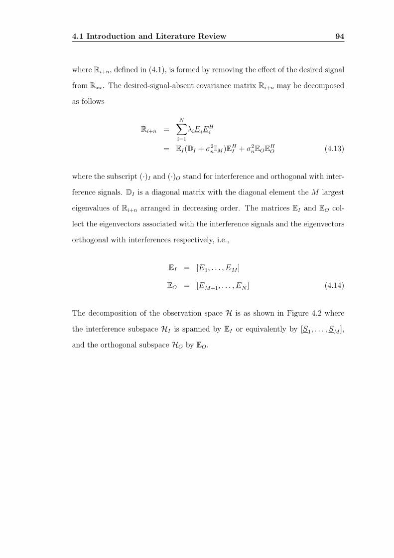
4.1 Introduction and Literature Review 94
where Ri+n, defined in (4.1), is formed by removing the effect of the desired signal
from Rxx. The desired-signal-absent covariance matrix Ri+n may be decomposed
as follows
Ri+n =N∑i=1
λiEiEHi
= EI(DI + σ2nIM)EH
I + σ2nEOEH
O (4.13)
where the subscript (·)I and (·)O stand for interference and orthogonal with inter-
ference signals. DI is a diagonal matrix with the diagonal element the M largest
eigenvalues of Ri+n arranged in decreasing order. The matrices EI and EO col-
lect the eigenvectors associated with the interference signals and the eigenvectors
orthogonal with interferences respectively, i.e.,
EI = [E1, . . . , EM ]
EO = [EM+1, . . . , EN ] (4.14)
The decomposition of the observation space H is as shown in Figure 4.2 where
the interference subspace HI is spanned by EI or equivalently by [S1, . . . , SM ],
and the orthogonal subspace HO by EO.

4.1 Introduction and Literature Review 95
Origin
Desired Signal Subspace
Interference Subspace (dim= )M
-dimN
observation space
complex
H LI= [ , ..., ]S1
L[ ]= ,I S S2 M
L[ ]Sd (dim=1)
Noise Subspace
HO=L[ ]O (dim= )N-M
ψ
Figure 4.2: Decomposition of the space spanned by the columns of the data
covariance matrix when the desired signal is absent
Following the same analysis as with Wiener-Hopf, the optimum weight will
be given by a similar equation to that of Eq.(4.8) but now the term σ−2n PEO
U s
is not zero, i.e., σ−2n PEO
U s = 0. Then it can be shown that, in the absence of
any interferences and taking into accounting that EO spans the whole observation
space, the projection operator applied to any vector belonging to that space leaves
it unchanged. That is
PEOSd = Sd and PEO
U s = U s (4.15)

4.1 Introduction and Literature Review 96
which implies that Pdout = σ2
d
(UH
s Sd
σ2n
)2PIout = 0
Pnout =|Us|
2
σ2n
(4.16)
It is obvious from Eq.(4.16) that now the desired output at the output of
the array is proportional to that at the input, so the power inversion problem is
avoided.
When the pointing errors are absent (U s = Sd) and the matrix inverse
lemma [22] is used, one has
wWH = R−1xxSd
=(Ri+n+σ
2dSdS
Hd
)−1Sd
=
(R−1
i+n−R−1
i+nσ2dSdS
Hd R−1
i+n
1 + σ2dS
Hd R−1
i+nSd
)Sd
=1
1 + σ2dS
Hd R−1
i+nSd︸ ︷︷ ︸scalar
R−1i+nSd (4.17)
The above shows that the weight vectors of the “full” and “modified”Wiener-Hopf
processors differ only by a scalar factor and therefore offer identical maximum
SNIR at the output if pointing errors are absent.
Now considering the presence of pointing errors, the output array SNIRs
of both full and modified Wiener-Hopf processors can be expressed as [52]
SNIRWH out =σ2dS
Hd R−1
i+nSd cos2 Ψ
1 +[2σ2
dSHd R−1
i+nSd + (σ2dS
Hd R−1
i+nSd)2]sin2Ψ
SNIRm-WH out = σ2dS
Hd R−1
i+nSd cos2 Ψ (4.18)

4.1 Introduction and Literature Review 97
with
cos2 Ψ∆=
∥∥UHs R−1
i+nSd
∥∥2∥∥UHs R−1
i+nU s
∥∥∥∥SHd R−1
i+nSd
∥∥sin2 Ψ
∆= 1− cos2 Ψ (4.19)
where Ψ can be viewed as the generalized angle between the vector U s and Sd.
In the presence of pointing errors, cos2Ψ < 1 and thus the output SNIRs of
the both processors degrade. However, it can be seen clearly from (4.18) that
the degradation of the modified Wiener-Hopf processor is much less than that
of the full Wiener-Hopf processor if the term σ2dS
Hd R−1
i+nSd is greater than unity.
Thus, the modified Wiener-Hopf outperforms the full Wiener-Hopf in terms of
the robustness to pointing errors.
However, both full and modified Wiener-Hopf always allow interference
to pass at the output of an array of sensors, thus contaminating the desired
signal. For this reason, the weight-vectors provided by these processors are not
appropriate for complete interference cancellation.
4.1.3 Robust Techniques for Wiener-Hopf processors
In order to enhance the robustness of Wiener-Hopf processors (or Capon Beam-
formers), the popular diagonal loading (DL) method has been presented in [53]
with the weight vector given by
wDL =(Rxx + µI)−1U s
UHs (Rxx + µI)−1U s
(4.20)
4.1 Introduction and Literature Review 98
where the pointing vector U s = Sd generally. Actually, the above is the solution
for the following optimum problem
minw
wHRxxw + µwHw subject to wHU s = 1 (4.21)
In comparison with standard Capon problem in (4.6), an additional penalty term
µwHw is imposed on the objective function of the above DL problem. Thus
the positive loading factor µ > 0 can penalize large values of w and detune
the beamformer response around the nominal U s [45]. However, there is no
systematic approach to choose the loading factor µ. Usually, µ is set in an ad hoc
way, typically 10σ2n. Another drawback of the conventional DL is that there exists
potential risk at over-penalizing the uncertainty of Rxx (because of the quadratic
term wHRxxw in (4.21)) [54].
In recent years, the generalized versions of the DL, or called robust Capon
beamformers (RCB), have been studied in [44, 45, 55–59], in which the diagonal
loading factor is related to the uncertainty level and can be related to the un-
certainty level. Among them, the RCB developed in [44] is the most influential,
which can be stated by the following problem
minS
SHR−1xxS subject to ∥S − U s∥
2 ≤ ϵ (4.22)
where the uncertainty level ϵ is a preselected constant satisfying
∥Sd − U s∥2 ≤ ϵ (4.23)
The objective function in the above optimum problem is designed to minimize
the output power of the Capon beamformer.
It is difficult to solve the above optimum problem directly because the

4.1 Introduction and Literature Review 99
spherical constraint set is infinite. However, the optimal solution S⋆ must occur on
the boundary of the constraint set, i.e., ∥S⋆ − U s∥2 = ϵ. This can be understood
by the following contradiction. Suppose that ∥S⋆ − U s∥2 = ϵ1 < ϵ, then there
exists a ν ∈ (0, 1) such that
∥νS⋆ − U s∥2 = ∥(S⋆ − U s) + (ν − 1)S⋆∥2
≤ (∥S⋆ − U s∥+ (1− ν) ∥S⋆∥)2
= (√ϵ1 + (1− ν) ∥S⋆∥)2 (4.24)
If ν is close to unity sufficiently, we can obtain ∥νS⋆ − U s∥2 ≤ ϵ, which means
νS⋆ also belongs to the spherical constraint. Then,
(νS⋆)HR−1xx (νS
⋆) = ν2S⋆HR−1xxS
⋆ < S⋆HR−1xxS
⋆ (4.25)
The above means that one can find a vector in the constraint set, νS⋆, which
makes the objective function in (4.22) less than that corresponding to S⋆. How-
ever, this is impossible because S⋆ is assumed to be the optimal solution and corre-
sponds to the minimum of the objective function. Thus S⋆ has to be a boundary
point of the spherical constraint. Therefore, the infinite number of inequality
constraints in (4.22) is transformed into a single constraint (i.e., ∥S − U s∥2 = ϵ).
Then the Lagrange multiplier methodology can be utilized to find the optimal
solution. The associated weight vector may be expressed as
wRCB =R−1
xxS⋆
S⋆HR−1xxS
⋆(4.26)
Interestingly, the RCB presented in [44] provides an equivalent solution to
that in [57] and [45] where the convex optimization techniques are utilized.
4.1 Introduction and Literature Review 100
It is evident that the solution S⋆ will no longer collinear to Sd, even when
the actual value of Sd is used in (4.22) instead of U s [60]. Moreover, if a point
is moved along the constraint boundary, the optimal solution S⋆ should be the
point closest to the principal eigenvector of Rxx. This implies that S⋆ is definitely
affected by the interference signals because the principal eigenvector is a linear
combination of all the manifold vectors (both the desired and the interferences).
This situation would become worse when the DOAs of some interferences are
close to the desired DOA, since the interference manifold vector may contribute
significantly to the principal vector. In [60], a method based on multi-dimensional
covariance fitting is presented to overcome the above problems. However, this
method requires the knowledge of all the manifold vectors (including both the
desired and the interference signals) and the associated uncertainty sets.
In [61–65] the method of signal-subspace projection (SSP) has been inves-
tigated for reducing the manifold mismatch, in which the presumed manifold is
replaced with its projection onto the signal subspace. That is
wSSP = R−1xxPEsU s (4.27)
Unfortunately this projection operation cannot eliminate the mismatch lying in
the signal subspace. Also, both RCB and SSP are not an interference cancellation
technique and hence the interferences can pass through the beamformers.
4.1.4 Blocking Matrix Approaches
Blocking matrix approaches [66–69] attempt to remove the effects of the desired
signals by using a spatial blocking filter, as illustrated in Figure 4.3. The spatial
4.1 Introduction and Literature Review 101
blocking matrix B ∈ CN×(N−q) has the following properties
BHSd = 0
BHSi = ciS(q)i i = 1, . . . ,M (4.28)
where ci is a complex constant, and S(q)i denotes the vector consisting of the first
(N − q) elements of Si. (4.28) means that the blocking matrix B is orthogo-
nal to the manifold of the desired signal and hence the desired signal is blocked
completely. In addition, the interferences can pass the spatial filter with dimen-
sionality reduction by q. Let xB ∈ C(N−q) denote the signal at the output of the
spatial filter, which is given by
xB = BHx(t)
=M∑i=1
cimi(t)S(q)i + BHn(t) (4.29)
Thus the interference subspace can be found by computing the M dominant
eigenvectors of the covariance matrix RB = ExB(t)xHB (t). The weight vector
w is obtained by projecting Sd onto the complement subspace of the interference
subspace, which aims to cancel the interferences totally. Finally the received
signal at the first N − q sensors, i.e., x(q)(t) = [x1(t), x2(t), . . . , xN−q(t)]T , is
weighted by w to reproduce the desired signal.

4.1 Introduction and Literature Review 102
( ) ∈Nx t C
( )( ) ( )H N q
Bx t x t −= ∈
( )−∈
N qw C
( )× −∈
N N qC
Spatial blocking Filter
Form and
perform eigen-decomposition
( ) ( )− × −∈
N q N q
blk C
Construct weight vector
by projecting the desired
manifold onto
the interference
complement subspace
×
( )( )
qx t
array output
1 2 −N q N
( )y t
( ) ( )( ) −∈
q N qx t C
( ) 1− ×N q
Figure 4.3: The structure of the beamformer using blocking matrix

4.1 Introduction and Literature Review 103
For the simple case where q = 1, the structure of the spatial blocking filter
is depicted in Figure 4.4, where D is the distance between two adjacent sensors
and the corresponding blocking matrix can be expressed as
B =
−1, 1, 0, · · · , 0, 0
0, −1, 1, · · · , 0, 0
......
.... . .
......
0, 0, 0, · · · , −1, 1
(4.30)
For the design details of B with general q, see [67, 68]. Note that all the designs
are derived strictly under the uniform linear array (ULA) assumption.
( ) ∈Nx t C
( )( 1)( ) ( ) ( )H N
B dx t S x tθ−
= ∈
Spatial Blocking Filter
×
1 2 N
cos dje
π θD
− − −
1N −3
×2 cos dj
eπ θD
×( 2) cos dj N
eπ θ− D
×( 1) cos dj N
eπ θ− D
Figure 4.4: An example of spatial blocking filter with q = 1
4.1 Introduction and Literature Review 104
By subtracting the received signals, the dimensionality of the observation
space is reduced. For instance, the dimensionality is reduced by q in Figure 4.3.
In turn, this implies a reduction in resolution and SNIRout. Furthermore, the ap-
proaches are strictly limited to ULA because the matrix B is derived on the basis
of ULAs. In the presence of pointing errors, the desired signal will leak into the
output of the blocking matrix, which may result in the severe performance degra-
dation since the desired signal would be contained in the interference subspace
and therefore be suppressed instead of being enhanced.
4.1.5 Problem Statement
On the basis of the above discussion, it is clear that the conventional Wiener-Hopf
(or the Capon) beamformers suffer from the power inversion problem and lack of
the robustness to the pointing errors. The existing robust Capon beamformers
cannot work efficiently in many cases and allow the interferences to pass as well.
Though the modified Wiener-Hopf overcome the power inversion problem and
has the robustness to the pointing errors, the optimum weights for maximization
of SNIR always allows interferences to pass to the output of the array. The block-
ing matrix methods achieve the complete cancellation of the interferences, but it
cannot be applied in arrays with non-ULA geometries and it has the potential
to cancel the desired signal in the presence of pointing errors. The problem to
be addressed, in this chapter, is to find a unified solution which not only pre-
vents power inversion and reduces the effect of pointing error but also provides,
asymptotically, complete interference rejection that is lack in conventional beam-
formers.
4.2 Proposed Interference Cancellation Beamformer 105
4.2 Proposed Interference Cancellation Beam-
former
In the previous chapter, it is demonstrated that in the presence of the pointing
errors the actual manifold of the desired signal can be expressed as
Sd = Hb (4.31)
where the p× 1 linear combination vector b is unknown because Sd is not exactly
known due to the pointing errors. The matrix H is known or can be found easily,
which is formed using one of the following expressions in this chapter
H1 = [S0, S(θ0), S(θ0)]
H2 = [S(θ0), S(θ0 −∆θ), S(θ0 +∆θ)] (4.32)
where S(θ0) and S(θ0) denote the first and second derivatives with respect to the
presumed DOA θ0. ∆θ is related to the expected range of the DOA of the desired
signal and can be set even if the actual DOA is unavailable.
It also assumes that [H S1, . . . , SM ] is full column rank, which implies that
the columns of [H S1, . . . , SM ] are linearly independent. Moreover, the rank of
[H S1, . . . , SM ] is less than N . The pointing vector is not equal to the actual
manifold, i.e., U s = S(θ0) = Sd (or written as U s = S0 = Sd).
Also, it is well known that the manifold vectors of all signals, including the
desired signal and the interference signals, should belong to the so-called signal
subspace L[Es] which can be obtained by performing eigen-decomposition on the
covariance matrix Rxx (see Eq.(4.4)).
Now two different subspaces associated with the desired signal are at hand
4.2 Proposed Interference Cancellation Beamformer 106
and thus it is intended to make the most of these information to remove the effects
of the pointing errors as much as possible.
4.2.1 Estimate Using Vector Subspace Projections (VSP)
The approach proposed to eliminate the pointing errors applies the theorem of
sequential VSP to find the intersection of the two constraint subspace. The
simplest form of VSP, suggested by von Neumann in [70], is the alternating
projection in which the iterative projections are performed to find the intersection
of two Hilbert subspace. This work has been generalized for more than two
closed subspaces and also for convex sets by Stark and Yang [71] so that the VSP
method has found applications to a wide range of practical engineering problems.
The applications of the projection methods to array signal processing have been
considered in [72–75]. A fundamental theorem of VSP states the following:
Theorem 4.1 [71]: Let C1, C2, . . . ,Cm represent m closed convex sets in a
Hilbert space H, and let PCi denote the projection onto Ci, i = 1, . . . ,m. If the
intersection C0=∩m
i=1 Ci is non-empty and the dimension of H is finite, then the
sequence (PC1PC2 . . .PCm)ka0 converges strongly to a point in the solution set C0,
PC0a0, for every non-zero point a0 ∈ H.
Proof: [71]
To place this theorem in the context of the pointing error elimination, the
key is how to define the appropriate constraint sets Ci to describe the available
information. Under the above assumptions, two constraints can now be imposed
on Sd.
C1 = S : S ∈ L[Es] (4.33a)
C2 = S : S ∈ L[H] (4.33b)
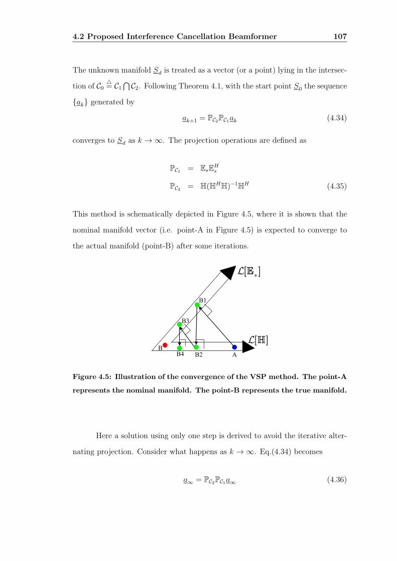
4.2 Proposed Interference Cancellation Beamformer 107
The unknown manifold Sd is treated as a vector (or a point) lying in the intersec-
tion of C0= C1
∩C2. Following Theorem 4.1, with the start point S0 the sequence
ak generated by
ak+1 = PC2PC1ak (4.34)
converges to Sd as k → ∞. The projection operations are defined as
PC1 = EsEHs
PC2 = H(HHH)−1HH (4.35)
This method is schematically depicted in Figure 4.5, where it is shown that the
nominal manifold vector (i.e. point-A in Figure 4.5) is expected to converge to
the actual manifold (point-B) after some iterations.
[ ]L
[ ]s
L
A
B
B1
B2
B3
B4
Figure 4.5: Illustration of the convergence of the VSP method. The point-A
represents the nominal manifold. The point-B represents the true manifold.
Here a solution using only one step is derived to avoid the iterative alter-
nating projection. Consider what happens as k → ∞. Eq.(4.34) becomes
a∞ = PC2PC1a∞ (4.36)

4.2 Proposed Interference Cancellation Beamformer 108
The above equation implies that the final converged estimate a∞ is given by the
eigenvector (up to a scaling factor) of matrix PC2PC1 which has a corresponding
eigenvalue equal to one. Also, the maximum eigenvalue of the matrix product
PC2PC1 is one. In accordance with Corollary 11 of [76], one obtains
eigmax(PC2PC1) ≤ eigmax(PC2) maxu
uHu=1
uHPC1u
= maxu
uHu=1
uHPC1u
uHu
= eigmax(PC1)
= 1 (4.37)
where the fact that the maximum eigenvalues of the PC1 and PC2 are one is used in
the above. The notation eigmax(A) denotes the maximum eigenvalue of A. Hence
if the nominal θ0 and Es are given, instead of S0, the steering vector used is given
by
U s = βPPC2PC1 (4.38)
where β is chosen such that ∥U s∥2 = N .
4.2.2 Power Estimator
In [77], the power of the desired signal is estimated by searching the minimum
of a cost function. The basic idea is that a temporary matrix R(α) is formed by
removing the noise effect and subtracting the effect of the desired signal with a
real variable factor α from Rxx, i.e.,
R(α) = Rxx − σ2nI− αSdS
Hd (4.39)
4.2 Proposed Interference Cancellation Beamformer 109
Then the estimated power is the largest possible value of α, which maintains R(α)
semipositive (for details, see Appendix 4.A). However, searching the minimum of
the cost function may involve expensive computations because a number of eigen-
decomposition operations are required.
In [55], the power estimation is solved by using covariance fitting theory,
which can be expressed as follows
σ2d =
1
SHd R−1
xxSd
(4.40)
Clearly the computation complexity is quite low because only one step is needed.
Nevertheless the effect of noise on the signal subspace is neglected. This can
be seen in the case where the interferences are absent. The covariance matrix
becomes Rxx = σ2dSdS
Hd + σ2
nIN and its inverse is readily obtained
R−1xx =
INσ2n
− σ2d
σ2n(σ
2n +Nσ2
d)SdS
Hd (4.41)
Then the power estimation using (4.40) is given by
σ2d = σ2
d +σ2n
N= σ2
d (4.42)
Here a single step power estimation is proposed in which the effect of noise
on the signal subspace is taken into account. The power of the desired signal σ2d

4.2 Proposed Interference Cancellation Beamformer 110
is equivalent to the largest possible value of σ2 which satisfies
eigi(Rxx − σ2SdS
Hd
)≥ σ2
n, ∀i
⇔ eigi(Rxx − σ2
nIN − σ2SdSHd
)≥ 0, ∀i
⇔ eigi(EH
s (Rxx − σ2nIN)Es − σ2EH
s SdSHd Es
)≥ 0, ∀i
⇔ eigi(Ds − σ2EH
s SdSHd Es
)≥ 0, ∀i
⇔ eigi
(IM+1 − σ2D− 1
2s EH
s SdSHd EsD
− 12
s
)≥ 0, ∀i
⇔ 1− σ2SHd EsDs
−1EHs Sd ≥ 0
⇔ σ2 ≤ 1
SHd EsD−1
s EHs Sd
(4.43)
where D−1/2s denotes Hermitian square root of D−1
s . The notation eigi(A)
represents the ith largest eigenvalue of A. In the above derivation, the fact
that D− 12
s EHs SdS
Hd E
−1/2s D− 1
2s is a rank-one matrix with the principal eigenvalue
SHd EsD−1
s EHs Sd is used. Hence the power of the desired signal is
σ2d =
1
SHd EsD−1
s EHs Sd
(4.44)
Let us examine the interference-absent case again. Ds becomes a scalar
equal to Nσ2d, and S
Hd EsEH
s Sd = N . Thus (4.44) offers the precise power estima-
tion.
The proposed method obtains the same power estimation as the approach
in [77] but with much less computational complexity. Interestingly, [78] (see
Lemma III.1 of [78]) proposed the equivalent power estimation method from the
viewpoint of the oblique projection.

4.2 Proposed Interference Cancellation Beamformer 111
4.2.3 Beamformer Construction
In the previous section, it has been seen that the modified Wiener-Hopf processor
solves the power inversion problem through removing the desired signal effect
from the covariance matrix. The proposed processor estimates and subtracts the
desired signal effects to form the desired-signal-absent covariance matrix given by
Ri+n = Rxx − σ2dU s(U s)
H (4.45)
where U s is obtained by Eq.(4.38) using the VSP method, the power σ2d is com-
puted by Eq.(4.44) using the modified one step power estimation method where
Sd is replaced by U s.
Performing eigen-decomposition on Ri+n yields
Ri+n =N∑i=1
λiEiEH
i
= EI(DI + σ2nIM)EH
I + σ2nEOEH
O (4.46)
Now the interference subspace HI spanned by [S1, . . . , SM ] is equivalent to the
subspace spanned by EI . Let P⊥I be the orthogonal projection operator of the
interference subspace. Then P⊥I can be estimated by
P⊥I = I− EIEH
I (4.47)
The proposed interference cancellation weight vector is expressed as
wic =P⊥I U s√
UH
s P⊥I U s
(4.48)
The jammer power at the array output, using the actual DOA of the desired
4.2 Proposed Interference Cancellation Beamformer 112
signal, will be zero because wic is orthogonal with the interference subspace. The
total output power of the array becomes
Pout = σ2dS
Hd P⊥
I Sd + σ2n (4.49)
where the first term in the right is proportional to the input power of the desired
signal. It is clear that the proposed method does not suffer from the power
inversion problem. The SNR at the array output will be:
SNRout =σ2d
σ2n
SHd P⊥
I Sd (4.50)
The angle between the Hd (the subspace spanned the desired signal) and
H⊥I subspaces, ψ, is defined as
ψ = arccos
√SHd P⊥
I Sd√SHd Sd
(4.51)
Therefore, Eq.(4.50) is equivalent to:
SNRout =σ2d
σ2n
(SHd Sd) cos
2 ψ =σ2d
σ2n
N cos2 ψ (4.52)
Eq.(4.52) shows that the ability of the proposed beamformer to completely cancel
the interferences is obtained at the cost of SNIR degradation or partial cancella-
tion of the desired signal. If there is an interference very close to the desired signal
direction then ψ → 90 and the output SNR deteriorates significantly, which may
result in an unacceptable tradeoff. However, this undesirable property is not re-
stricted to the proposed processor. The Wiener-Hopf processor (and all other
known processes) also suffers from this restriction when interferences are located
close to the desired signal direction.

4.3 Performance Analysis in the Presence of Pointing Errors 113
4.2.4 Proposed Algorithm
The proposed algorithm can be presented as a series of steps as follows:
1. Estimate the data covariance matrix Rxx. Find its signal subspace eigen-
vectors Es and compute the projection operator PC1 .
2. Calculate the H using the nominal DOA θ0 and form the projection operator
PC2 .
3. Estimate the steering vector U s using Eq.(4.38) and the power σ2d using
Eq.(4.44) with Sd replaced by U s.
4. Estimate the matrix Ri+n by Eq.(4.45).
5. Perform eigen-decomposition on the matrix Ri+n. Find the projection op-
erator P⊥I using Eq.(4.47).
6. Compute the weight vector wic using Eq.(4.48).
7. Weight the inputs of the array with wic.
4.3 Performance Analysis in the Presence of
Pointing Errors
Now consider the case U s = Sd, i.e., there is a mismatch between the steering
vector and the real manifold vector of the desired signal. Then the desired-signal-
absent covariance matrix contains some perturbations as depicted in Figure 4.6,

4.3 Performance Analysis in the Presence of Pointing Errors 114
i.e.,
Ri+n = Rxx − σ2dU s(U s)
H
= Ri+n + (σ2dSdS
Hd − σ2
dU s(U s)H)︸ ︷︷ ︸
=Ri+n
(4.53)
where the perturbation term Ri+n is a rank-2 matrix if U s = Sd.
[ ]dSL
ψ
[ ]s
UL
ψ
Origin
H H
H
H
Figure 4.6: Decomposition of the space by the columns of Ri+n
Using the first-order subspace perturbation theory [79], the perturbed sig-
nal eigenvectors is given by
EI = EI + EOEHO RH
i+nEID−1I︸ ︷︷ ︸
=EI
(4.54)
where EO and EI are the noise-subspace eigenvectors and signal-subspace eigen-
vectors of the actual desired-signal-absent covariance matrix Ri+n. Then the
4.3 Performance Analysis in the Presence of Pointing Errors 115
perturbed orthogonal projection operator can be expressed by
P⊥I = I− EIEH
I
= P⊥I + EIEH
I + EIEHI + EIEH
I︸ ︷︷ ︸=P⊥
I
(4.55)
Substituting the above into Eq.(4.48) yields
wic =P⊥I U s∣∣∣P⊥I U s
∣∣∣2 (4.56)
Now the output interference power, PIout , no longer equals zero due to pointing
errors, because the weight vector is not orthogonal with the interference manifold,
i.e., wHicSi = 0.
Consequently SNIRout in the presence of pointing errors can be given by
SNIRout =σ2d
∣∣wHicSd
∣∣2PIout + σ2
n
∣∣wHic wic
∣∣=
σ2d
∣∣∣UH
s P⊥I Sd
∣∣∣2M∑i=1
σ2i
∣∣∣UH
s P⊥I Si
∣∣∣2 + σ2n
∣∣∣UH
s P⊥I U s
∣∣∣=
σ2dN cos2 ψ
M∑i=1
σ2i
∣∣∣UH
s P⊥I Si
∣∣∣2∣∣∣UH
s P⊥I Us
∣∣∣ + σ2n
(4.57)
where ψ denotes the angle between Sd and P⊥I U s. When the pointing errors are
absent, the perturbation term P⊥I is a matrix of zeros and ψ equals to ψ, which
means the above equation reduces to Eq.(4.52).

4.4 Simulation Studies 116
4.4 Simulation Studies
Assume that one desired signal and three interferences impinge on a ULA with
N = 10 isotropic sensors and half-wavelength sensor spacing. Note that the pro-
posed algorithms is applicable to arbitrary array geometry although here ULA
array is used. The desired signal’s DOA is fixed at 90 in all the following exam-
ples. All signals have unit power. Noise power is σ2n = 0.1 (-10dB). The matrix
H is composed of three columns (the nominal manifold vector and its first two
derivatives with respect to the DOA. See Eq.(3.6)).
Case 1: In the first example, the DOAs of interference are at 60, 62 and 70.
The pointing angle is 90 (i.e., no pointing error in this example). The array pat-
terns of three methods (Wiener-Hopf, Lee-Lee [68] and the proposed) are shown
in Figure 4.7, where Lee-Lee’s method is one of the blocking matrix methods.
It can be seen in Figure 4.7 that by using the Wiener-Hopf processor it is not
possible to distinguish (resolve) the two closely spaced interfering sources (60
and 62) correctly whereas it is possible with the processor based on the pro-
posed wic or on Lee-Lee’s weight. Also, both Lee-Lee’s method and the proposed
method present very deep nulls at the locations of the unknown interferences
while they provide a free way to the desired signal. An added advantage is that
each deep null provides the location estimate of an unknown interference, because
these deep nulls are easily distinguishable from the rest of the array pattern. It
can also be seen in Figure 4.7 that Wiener-Hopf allows the interference to pass
through partially because the associated array pattern cannot place deep nulls at
the locations of interferences. The power estimations of the three methods are
listed in Table 4.1 which illustrates that the proposed method, with much less
computational complexity, provides the precise estimate as well as [77], whereas
there exists the estimation error in [55].

4.4 Simulation Studies 117
0 20 40 60 80 100 120 140 160 180−350
−300
−250
−200
−150
−100
−50
0
50
Azimuth (degrees)
Arr
ay P
atte
rn (
dB)
Wiener−Hopf
Lee−LeeProposedProcessor
Figure 4.7: Array pattern with two interferences close together (60 and
62). The DOA of the desired signal is 90.
Table 4.1: Estimated power of the desired signal
actual power Proposed Ref. [77] Ref. [55]1 1 1 1.0191
Case 2: Comparison is made with respect to pointing error effects in the Wiener-
Hopf (“modified” and “full” version), proposed processor and Lee-Lee processor in
the second example. The DOAs of interferences are 70, 80 and 100. Though
Figure 4.8 shows that the proposed processor is more susceptible to pointing
errors than the “modified” Wiener-Hopf solution, it performs much better than
the Lee-Lee and “full” Wiener-Hopf processors. The SNIR of Lee-Lee without

4.4 Simulation Studies 118
pointing error is below the optimum SNIR. This is because the dimensionality of
the observation space is reduced in the Lee-Lee processor to construct the blocking
matrix. In addition, Table 4.2 shows that the results computed by the analytical
equations in previous section are consistent with the simulation results when the
pointing errors are small. If the pointing error is over 4, the approximation
in Eq.(4.54) in the sense of the first-order subspace perturbation is invalid and
therefore there are significant mismatches between the simulation results and the
theoretical analysis.
−5 −4 −3 −2 −1 0 1 2 3 4 50
2
4
6
8
10
12
14
16
18
20
Point Error (degrees)
SN
IR (
dB)
mod−Wiener−HopfWiener−HopfLee−LeeProposed method
Figure 4.8: Effects of pointing errors with noise level at -10dB. The true
direction of the desired signal maintained at 90.

4.4 Simulation Studies 119
Table 4.2: SNIRout (unit: dB) with noise level at -10dB
pointing angle SNIRout by simulation SNIRout by Eq.(4.57)
850 0 8.12
860 9.64 10.10
870 17.44 16.86
880 19.46 19.41
890 19.55 19.55
900 19.55 19.55
910 19.55 19.55
920 19.51 19.49
930 18.89 18.59
940 14.68 13.90
950 5.86 7.74
Case 3: In the third example, three other existing robust beamformers are
also simulated in the same environment as the second example. The first robust
algorithm is the conventional DL [53] with the diagonal loading factor ξ = 10σ2n
(see Eq.(4.20)). The second method is the SSP method proposed in [61] and its
weight vector is given by
wssp = R−1xxPC1S(θ0) (4.58)
Two different RCBs (with the spherical constraint and with flat ellipsoidal con-
strain) presented in [44] are examined. The legend RCB-1 in Fig.4.9 stands
for the RCB with the spherical constraint. Here the spherical boundary ϵ
(∥S(θd) − S(θ0)∥2 ≤ ϵ) is equal to the larger of ∥S(θ0) − S(θ0 − ∆θ)∥2 and
∥S(θ0)−S(θ0+∆θ)∥2, where ∆θ = |θ0− θd|+0.5. The legend RCB-2 in Fig.4.9
means the RCB with flat ellipsoidal constrain. In previous chapter it has been
shown that the flat ellipsoidal uncertainty set in [44] can be viewed as an ex-

4.4 Simulation Studies 120
ample of the uncertainty model used in this thesis. Setting B = [S(θ0), S(θ0)],
the condition that SH(θ0)(B†)HB†S(θ0) > 1 (where † denotes the Moore-Penrose
pseudo-inverse) does not hold. This means that RCB with B = [S(θ0), S(θ0)] fails
(see (45) of [44]). In order to satisfy this condition and simulate the second RCB
method, B is set to be B = [S(θ0)−S(θ0−∆θ), S(θ0)−S(θ0+∆θ)] The legends
Proposed-1 and Proposed-2 in Figure 4.9 represent the proposed method using
H1 = [S(θ0), S(θ0), S(θ0)] andH2 = [S(θ0), S(θ0)−S(θ0−∆θ), S(θ0)−S(θ0+∆θ)]
respectively. Figure 4.9 shows that the proposed method outperforms the other
three methods when pointing errors happen. In addition, the proposed method
is applicable to more practical applications than the RCB with flat ellipsoidal
constraint because the condition SH(θ0)(B†)HB†S(θ0) > 1 is relaxed.
−5 −4 −3 −2 −1 0 1 2 3 4 50
2
4
6
8
10
12
14
16
18
20
Point Error (degrees)
SN
IR (
dB)
mod Wiener−HopfDLSSPRCB−1RCB−2Proposed−1Proposed−2
Figure 4.9: Effects of pointing errors. The true direction of the desired
signal maintained at 90.
Case 4: Finally, the effect of finite snapshots is tested. The simulation environ-
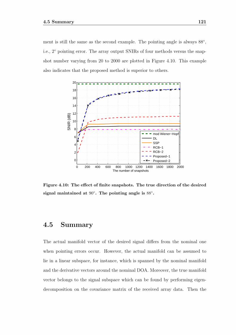
4.5 Summary 121
ment is still the same as the second example. The pointing angle is always 88,
i.e., 2 pointing error. The array output SNIRs of four methods versus the snap-
shot number varying from 20 to 2000 are plotted in Figure 4.10. This example
also indicates that the proposed method is superior to others.
0 200 400 600 800 1000 1200 1400 1600 1800 2000
0
2
4
6
8
10
12
14
16
18
20
The number of snapshots
SN
IR (
dB)
mod Wiener−HopfDLSSPRCB−1RCB−2Proposed−1Proposed−2
Figure 4.10: The effect of finite snapshots. The true direction of the desired
signal maintained at 90. The pointing angle is 88.
4.5 Summary
The actual manifold vector of the desired signal differs from the nominal one
when pointing errors occur. However, the actual manifold can be assumed to
lie in a linear subspace, for instance, which is spanned by the nominal manifold
and the derivative vectors around the nominal DOA. Moreover, the true manifold
vector belongs to the signal subspace which can be found by performing eigen-
decomposition on the covariance matrix of the received array data. Then the
4.5 Summary 122
estimate of the desired signal manifold can be obtained using VSP, by means of
which much of the pointing error is eliminated. The power of the desired signal
can be computed in one step operation using the theory of covariance fitting.
The estimates of manifold and power of the desired signal are then utilized to
construct the proposed estimate-and-subtract interference canceller beamformer
in which the power inversion problem is avoided. In the absence of pointing
errors, the proposed beamformer can completely cancel the interferences at the
cost of SNIR degradation or partial cancellation of the desired signal.
The tasks accomplished by the proposed algorithm are summarized as
follows
• provides complete interference cancellation with the output of the array
consisting only of desired signal and thermal noise;
• provides reduced susceptibility to pointing errors and noise level;
• does not suffer from the power inversion problem.

4.6 Appendix 4.A Revisit the power estimation 123
4.6 Appendix 4.A Revisit the power estimation
In this section, the power estimator proposed in [77] is revisited. A cost function
ξ(α) is defined in [77] as
ξ(α) =N∑i=1
eigi>0
(1 + eigi(R(α))) + 10 log10
N∑i=1
eigi<0
|eigi (R (α))|
(4.59)
where the matrix R(α) is formed from Rxx by excising the effects of the noise and
the desired signal, i.e.,
R(α) = Rxx − σ2nIN − αSdS
Hd (4.60)
[77] argues that the power can be found by searching the minima of ξ(α) over
α. That is
σ2d = argmin
α(ξ(α)) (4.61)
However, [77] has not elaborated why this method can work. Next, the essence
of this method will be revealed.
Substituting Rxx in (4.1) to (4.60) produces
R(α) =M∑i=1
σ2i SiS
Hi + (σ2
d − α)SdSHd
= Ri + (σ2d − α)SdS
Hd (4.62)
where the matrix Ri=
M∑i=1
σ2i SiS
Hi has the eigenvalues
eig1(Ri) ≥ eig2(Ri) ≥ . . . ≥ eigM(Ri) > eigM+1(Ri) = . . . = eigN(Ri) = 0
(4.63)
This means that Ri has M positive eigenvalues and (N −M) null eigenvalues,
4.6 Appendix 4.A Revisit the power estimation 124
if the theoretical covariance matrix Rxx is used. In the case of α ≤ σ2d, R(α) is
a semipositive matrix and thus has no negative eigenvalues. Therefore, only the
first term in the right side of (4.59) affects ξ(α), and thus ξ(α) may be simplified
as
ξ(α ≤ σ2d) =
N∑i=1
eigi>0
(1 + eigi(R(α)))
= (M + 1) + tr(R(α))
= (M + 1) +NM∑i=1
σ2i +N(σ2
d − α) (4.64)
Obviously, ξ(α) monotonically decreases in the area α ∈ [0, σ2d].
Now consider the case of α > σ2d. Then σ2
d − α < 0. It is reasonable to
assume that R(α) is of rank-(M +1) because [Sd, S1, . . . , SM ] is linearly indepen-
dent. Hence R(α) has (M +1) non-zero eigenvalues. According to the interlacing
eigenvalue theorem 8.1.8 in [22], it is found that
eigN(R(α)) ≤ · · · ≤ eigM+1(R(α)) ≤ eigM+1(Ri) = 0 ≤ eigM(R(α)) ≤ · · · ≤ eig1(R(α))
(4.65)
which implies that the smallest eigenvalue, eigN(R(α)), must be a negative value
and all the other non-zero eigenvalues of R(α) are positive. Then the cost function
can be rewritten as
ξ(α > σ2d) =
M∑i=1
(1 + eigi(R(α))) + 10 log10 |eigN(R(α)| (4.66)
Suppose δ = α − σ2d > 0 is a sufficiently small value, then the
value of |eigN(R(α)| is much less than unity. This implies that the term
10 log10 |eigN(R(α)| would result in a sharp decrease. Then with the increase
of α, the eigenvalue eigN(R(α) becomes more negative. However, the absolute

4.6 Appendix 4.A Revisit the power estimation 125
value |eigN(R(α)| becomes larger. In turn, the 10 log10(·) factor would cause a
sharp increase, when 10 log10 |eigN(R(α)| dominates ξ(α).
In sum, in the area α ∈ [0, σ2d), the cost function ξ(α) monotonically
decreases and R(α) has (M + 1) positive eigenvalues. At the point α = σ2d,
ξ(α) reaches the first minima and R(α) has M positive eigenvalues only. When
α > σ2d, ξ(α) monotonically increases and R(α) has M positive eigenvalues and
one negative eigenvalue.

126
Chapter 5
Conclusions
THIS thesis has been concerned with two fundamental problems in the array
signal processing. The first problem is DOA estimation. For the arbitrary
arrays, the extended root-MUSIC obtains the DOA information by rooting a
polynomial and thus is categorized as a search-free DOA estimate methods. In
Chapter 2, three major approaches of the extended root-MUSIC are revisited
firstly. The problem that they face is the high computational complexity due to
the high order of the polynomial. In order to reduce the computational burden,
two different solutions are proposed. One is implemented in an iterative way and
another can be realized by scanning multiple circles in parallel. Both proposed
methods are insensible to the radial errors and therefore outperform the MUSIC-
type methods.
Chapter 3 and 4 focus on the design of beamformers robust to pointing
errors. The pointing errors make the presumed manifold different than the actual
manifold. However, a linear subspace can be found by using the knowledge of
the presumed manifold, which contains the actual manifold. A matched direction
beamforming (MDB) is presented in Chapter 3, which is robust to

5.1 List of Contributions 127
1. pointing errors,
2. overestimation of the signal subspace dimension.
However, this MDB beamformer cannot cancel the interference completely be-
cause it is of Wiener-Hopf type. In Chapter 4, a novel interference cancellation
beamformer is proposed, which provides a unified solution to the problems of
1. power inversion,
2. the robustness to pointing errors,
3. complete interference cancellation.
Much of pointing errors is removed by using VSP projections. The power inver-
sion problem is avoided by excising all the effects of the desired signal from the
covariance matrix. The interference signals are completely cancelled at the array
output using a weight vector which is orthogonal with the interference subspace.
5.1 List of Contributions
The following list summarizes the main contributions of this thesis which are
supported by the publications given in page 7 of the thesis.
1. Proposal of a framework consisting of spectral factorization (using Schur
algorithm) and large eigenvalue finding (using Arnoldi iteration) to reduce
the computational complexity of the extended root-MUSIC. By exploiting
the properties that the roots appear in conjugate reciprocal pairs and the
roots of interest are closest to the unit circle, the proposed method computes
the desired roots only, implying a large number of the unwanted roots are
exempt from the calculation. (Chapter 2)

5.1 List of Contributions 128
2. Proposal of an IDFT-base root-MUSIC in which the root magnitude is ex-
plicitly modelled and the polynomial obtained by the extended root-MUSIC
is reformulated to a typical form of IDFT. The rooting process is avoided
by the implementation of multiple IDFT operations in parallel. (Chapter
2)
3. Development of a Wiener-Hopf type MDB beamformer which is robust to
pointing errors. The pointing errors result in the mismatch between the
nominal direction and the actual direction of the desired signal. This pro-
vides a mismatch between the corresponding manifold vectors (nominal
and true manifold vectors). However, a linear subspace containing the true
manifold vector can be found by using the knowledge of the nominal man-
ifold. Then the linear combination vector associated with true manifold
is equivalent to the principal eigenvector of a certain rank-1 matrix up to
scalar. Importantly, this rank-1 matrix is obtained without the recourse
to the knowledge of interference subspace. Moreover, it is found that the
proposed MDB is also robust to the overestimation of signal subspace di-
mension. (Chapter 3)
4. Development of a pointing error elimination method by using VSP projec-
tions. Two implementations are provided: the alternative iteration and a
single step solution. (Chapter 4)
5. Derivation of a single step subspace-type power estimator using the co-
variance fitting theory in which the noise effect is taken into account. It
enjoys both the high accuracy estimation and computational effectiveness.
(Chapter 4)
6. Proposal of a unified solution to the problems of power inversion, robust-

5.2 Suggestions for Further Work 129
ness to pointing errors, and complete interference cancellation. The desired-
signal-absent covariance matrix is formed by excising the effects of the de-
sired signal where the estimations of the power and manifold vector are
utilized. The proposed weight vector is found by projecting the manifold of
the desired signal onto the complement of the interference subspace (which
is spanned by the signal vectors of the desired-signal-absent covariance ma-
trix). Performance analysis of the proposed interference cancellation beam-
former in the presence of pointing errors is also presented, where the sub-
space perturbation theory is used. An analytic expression of output SNIR
is derived, which is verified by the simulation results. (Chapter 4)
5.2 Suggestions for Further Work
A number of different problems associated with DOA estimation for arbitrary
arrays and beamformers robust to pointing errors have been investigated in this
thesis, but the following topics are still opened for additional research effort.
1. Two dimension DOA estimation for arbitrary arrays using root-MUSIC.
Almost all extended root-MUSIC algorithms aim at finding the azimuth
angle only and leave the elevation angle untouched. By using the manifold
separation technique (MST), the array manifold, which is the function of
both azimuth and elevation angles, can be modelled using spherical har-
monics. Then the MUSIC spatial spectrum can be written in polynomial
form. Thus each peak in the MUSIC spectrum corresponds to one root of
this polynomial, meaning that the 2-dimension DOA angles can be found
by rooting the polynomial instead of searching minima over (θ, ϕ) sphere.
However, the problem needed to address is how to find the roots in the

5.2 Suggestions for Further Work 130
2-dimension complex space ((exp(−jθ), exp(−jϕ), which can be viewed as
a 4-dimension real space). An immediate consequence is that the roots
are not isolated points but rather 2-dimension surfaces in the 4-dimension
space [19].
2. Extension of IQML/MODE to arbitrary arrays. The classical MUSIC and
root-MUSIC are subspace-based DOA estimations which can achieve the
performance as ML estimators (MLE) when the snapshot number is suffi-
ciently large and the signal sources are uncorrelated. However, when the
sources are coherent or the snapshot number is relatively small, the perfor-
mance of subspace-type estimators will suffer a degradation in comparison
with MLE. As stated in Chapter 2, a major drawback of ML methods is the
their computational intensity due to the requirement of multi-dimension
search. In order to reduce the computational complexity, the iterative
quadratic maximum likelihood (IQML) [80, 81] and the method of direc-
tion estimation (MODE) [82, 83] reformulate the multi-dimension search
into a problem of polynomial rooting. These two MLEs have the computa-
tional complexity comparable to that of MUSIC but better performance in
the case of highly correlated sources. However, these two MLEs are derived
under the assumption of ULA arrays. Hence the extension of these MLEs
to arbitrary arrays is attractive. In [84], MODE has been extended to arbi-
trary arrays using the technique of interpolated array. The main problem
of [84] is that the significant mapping errors are introduced, which degrades
the estimation performance. The MST technique cannot directly be used
for the extension because the matrix G(r) is not of full column rank but
of full row rank. The future works should provide the similar estimation
performance to the MLEs using ULA but with rather low computational
5.2 Suggestions for Further Work 131
burden.
3. Robust transceiver design. The robust techniques developed in this thesis
are applied at the receiver end. The transceiver may have a variety of struc-
tures. For instance, both the transmitter and receiver are equipped with
an an antenna array, which is called vector-in-vector-out (VIVO) system.
Also, the feedback from the receiver to the transmitter may contain partial
or full channel information. The robust transceiver may place the emphasis
on how the cooperation among the transceiver is designed to combat differ-
ent uncertainty types (such as pointing errors, moving sources, uncalibrated
array) in different situations.
4. Robust wideband array beamformer. In wireless communications, the high
data rate benefits from a wideband system. Using wideband signals in a
radar system leads to higher resolution than the narrowband counterpart.
However, the wideband applications violate the assumption that baseband
signal amplitudes at different sensors are approximately identical, which
renders the array manifold model for narrowband invalid. Generally the
tapped-delay-line structure is used at the receiver or/and the transmitter.
Thus the array system needs to handle in two domains (space-time pro-
cessing). In such case, robust wideband array beamformer is required to
overcome different uncertainty problems.

132
Bibliography
[1] D. H. Johnson and D. E. Dudgeon, Array Signal Processing: Concepts and
Techniques, PTR Prentice Hall, 1993.
[2] A. Manikas, Differential geometry in array processing, Imperial College
Press, 2004.
[3] M. Zatman, “How narrow is narrowband”, IEE Proceedings -Radar, Sonar
and Navigation, vol. 145, no. 2, pp. 85–91, 1998.
[4] J.E. Hudson, Adaptive Array Principles, Peter Peregrinus, 1981.
[5] V. Trees and L. Harry, Detection, estimation, and modulation theory. Part
4: Optimum array processing, Wiley-Interscience, 2002.
[6] H. Krim and M. Viberg, “Two decades of array signal processing research:
the parametric approach”, IEEE Signal Processing Magazine, vol. 13, no. 4,
pp. 67–94, 1996.
[7] L. C. Godara, “Application of antenna arrays to mobile communications
part ii: Beam-forming and direction-of-arrival considerations”, Proceedings
of the IEEE, vol. 85, no. 8, pp. 1195–1245, 1997.
[8] H. Cox, “Resolving power and sensitivity to mismatch of optimum array
processors”, The Journal of the Acoustical Society of America, vol. 54, no.
3, pp. 771–785, 1973.

Bibliography 133
[9] I. Ziskind and M. Wax, “Maximum likelihood localization of multiple sources
by alternating projection”, IEEE Trans. Acoustics, Speech and Signal Pro-
cessing, vol. 36, no. 10, pp. 1553 –1560, oct 1988.
[10] A. B. Gershman, M. Rbsamen, and M. Pesavento, “One- and two-
dimensional direction-of-arrival estimation: An overview of search-free tech-
niques”, Signal Processing, vol. 90, no. 5, pp. 1338 – 1349, 2010, Special
Section on Statistical Signal & Array Processing.
[11] R. Schmidt, Multiple emitter location and signal parameter estimation, PhD
thesis, Stanford University, 1981.
[12] R. Schmidt, “Multiple emitter location and signal parameter estimation”,
IEEE Trans. Antennas and Propag., vol. 34, no. 3, pp. 276–280, 1986.
[13] M. Rubsamen and A.B. Gershman, “Direction-of-arrival estimation for
nonuniform sensor arrays: From manifold separation to fourier domain mu-
sic methods”, IEEE Trans. Signal Process., vol. 57, no. 2, pp. 588–599, Feb.
2009.
[14] A. Paulraj, R. Roy, and T. Kailath, “A subspace rotation approach to signal
parameter estimation”, Proceedings of the IEEE, vol. 74, no. 7, pp. 1044 –
1046, july 1986.
[15] P. Stoica and A. Nehorai, “Performance comparison of subspace rotation
and music methods for direction estimation”, in Fifth ASSP Workshop on
Spectrum Estimation and Modeling, 1990., 10-12 1990, pp. 357 –361.
[16] A. Barabell, “Improving the resolution performance of eigenstructure-based
direction-finding algorithms”, in Proc. Int. Conf. Acoustics, Speech, Signal
Processing (ICASSP), Apr 1983, vol. 8, pp. 336–339.
Bibliography 134
[17] B.D. Rao and K.V.S. Hari, “Performance analysis of root-music”, IEEE
Trans. Acoust., Speech Signal Process., vol. 37, no. 12, pp. 1939–1949, Dec
1989.
[18] M.A. Doron and E. Doron, “Wavefield modeling and array processing. i.
spatial sampling”, IEEE Trans. Signal Process., vol. 42, no. 10, pp. 2549–
2559, Oct 1994.
[19] M.A. Doron and E. Doron, “Wavefield modeling and array processing .ii.
algorithms”, IEEE Trans. Signal Process., vol. 42, no. 10, pp. 2560–2570,
Oct 1994.
[20] M.A. Doron and E. Doron, “Wavefield modeling and array processing. iii.
resolution capacity”, IEEE Trans. Signal Process., vol. 42, no. 10, pp. 2571–
2580, Oct 1994.
[21] A. H. Sayed and T. Kailath, “A survey of spectral factorization methods”,
Numerical linear algebra with applications, vol. 8, no. 6-7, pp. 467–496, 2001.
[22] G. H. Golub and C. F. Van Loan, Matrix Computations, The Johns Hopkins
University Press, October 1996.
[23] I. Dacos and A. Manikas, “Eliminating the quantization problem in signal
subspace techniques”, IEICE Transactions on Communications, vol. E78-B,
no. 11, pp. 1458 – 1467, Nov. 1995.
[24] B. Friedlander, “The root-music algorithm for direction finding with inter-
polated arrays”, Signal Process., vol. 30, no. 1, pp. 15–29, 1993.
[25] P. Hyberg, M. Jansson, and B. Ottersten, “Array interpolation and bias
reduction”, IEEE Trans. Signal Processing, vol. 52, no. 10, pp. 2711 – 2720,
oct. 2004.

Bibliography 135
[26] P. Hyberg, M. Jansson, and B. Ottersten, “Array interpolation and doa mse
reduction”, IEEE Trans. Signal Processing, vol. 53, no. 12, pp. 4464 – 4471,
dec. 2005.
[27] F. Belloni, A. Richter, and V. Koivunen, “Doa estimation via manifold
separation for arbitrary array structures”, IEEE Trans. Signal Process., vol.
55, no. 10, pp. 4800–4810, Oct. 2007.
[28] Weisstein, Eric W. “Jacobi-Anger Expansion.” From MathWorld–
A Wolfram Web Resource. http://mathworld.wolfram.com/Jacobi-
AngerExpansion.html.
[29] Weisstein, Eric W. “Laurent Polynomial.” From MathWorld–A Wolfram
Web Resource. http://mathworld.wolfram.com/LaurentPolynomial.html.
[30] B. Sturmfels, Solving systems of polynomial equations, American Mathe-
matical Society,, 2002.
[31] D. C. Sorensen, “Numerical methods for large eigenvalue problems”, Acta
Numerica, Cambridge University Press, vol. 11, pp. 519–584, 2002.
[32] R. B. Lehoucq, D. C. Sorensen, and C. Yang, ARPACK users’ guide :
solution of large-scale eigenvalue problems with implicitly restarted Arnoldi
methods, Philadelphia : SIAM, 1997.
[33] T. Kailath, A. H. Sayed, and B. Hassibi, Linear Estimation, Prentice Hall,
1 edition, April 2000.
[34] K.V.S. Babu, “A fast algorithm for adaptive estimation of root-music polyno-
mial coefficients”, in in Proc. Int. Conf. Acoustics, Speech, Signal Processing
(ICASSP), Apr 1991, pp. 2229–2232 vol.3.
Bibliography 136
[35] P. Lemmerling, N. Mastronardi, and S. V. Huffel, “Fast algorithm for solv-
ing the hankel/toeplitz structured total least squares problem”, Numerical
Algorithms, Springer U.S., vol. Vol. 23, No. 4, pp. 371–392, 2000.
[36] G. S. Ammar and W. B. Gragg, “The generalized schur algorithm for the
superfast solution of toeplitz systems”, in in Rational Approximation and
its Applications in Mathematics and Physics. 1987, pp. 315–330, Springer.
[37] T. Kailath and A. H. Sayed, Eds., Fast reliable algorithms for matrices with
structure, Society for Industrial and Applied Mathematics, Philadelphia,
PA, USA, 1999.
[38] P. Bradley, C. Brennan, and M. Condon, “Arnoldi model order reduction for
electromagnetic wave scattering computation”, in International Conference
on Electromagnetics in Advanced Applications, 2007. ICEAA 2007, 17-21
2007, pp. 932 –935.
[39] J. Lee, V. Balakrishnan, C.-K. Koh, and D. Jiao, “From O(k2n) to O(n)
: A fast and high-capacity eigenvalue solver for full-wave extraction of very
large scale on-chip interconnects”, IEEE Trans. Microwave Theory and Tech-
niques, vol. 57, no. 12, pp. 3219 –3228, dec. 2009.
[40] O. Besson, L.L. Scharf, and F. Vincent, “Matched direction detectors and
estimators for array processing with subspace steering vector uncertainties”,
IEEE Trans. Signal Processing, vol. 53, no. 12, pp. 4453 – 4463, dec. 2005.
[41] A. Pezeshki, B. D. Van Veen, Louis L. Scharf, H. Cox, and M. L. Nordenvaad,
“Eigenvalue beamforming using a multirank mvdr beamformer and subspace
selection”, IEEE Trans. Signal Processing, vol. 56, no. 5, pp. 1954–1967,
2008.

Bibliography 137
[42] J. Li and P. Stoica, Eds., Robust Adaptive Beamforming, John Wiley &
Sons, 2005.
[43] M.H. Er and B.C. Ng, “A self-steered array system for microwave com-
munications”, IEEE Trans. Antennas and Propagation, vol. 42, no. 8, pp.
1192–1195, Aug 1994.
[44] J. Li, P. Stoica, and Z. Wang, “On robust capon beamforming and diagonal
loading”, IEEE Trans. Signal Process., vol. 51, no. 7, pp. 1702–1715, July
2003.
[45] R.G. Lorenz and S.P. Boyd, “Robust minimum variance beamforming”,
IEEE Trans. Signal Process., vol. 53, no. 5, pp. 1684–1696, May 2005.
[46] S. P. Boyd and L. Vandenberghe, Convex Optimization, Cambridge Univer-
sity Press, 2004.
[47] L. Griffiths and C. Jim, “An alternative approach to linearly constrained
adaptive beamforming”, IEEE Trans. Antennas and Propagation, vol. 30,
no. 1, pp. 27–34, 1982.
[48] L.L. Scharf and M.L. McCloud, “Blind adaptation of zero forcing projections
and oblique pseudo-inverses for subspace detection and estimation when in-
terference dominates noise”, IEEE Trans. Signal Processing, vol. 50, no. 12,
pp. 2938 – 2946, dec 2002.
[49] I. J. Gupta, “Performance of a modified applebaum adaptive array”, IEEE
Trans. Aerospace and Electronic Systems, vol. 20, pp. 583–594, 1984.
[50] R. A. Monzinco and T. W. Miller, Introduction to Adaptive Arrays, John-
Wiley, 1980.

Bibliography 138
[51] J. Capon, “High-resolution frequency-wavenumber spectrum analysis”, Pro-
ceedings of the IEEE, vol. 57, no. 8, pp. 1408–1418, 1969.
[52] O. L. Frost, “An algorithm for linearly constrained adaptive array process-
ing”, Proceedings of the IEEE, vol. 60, no. 8, pp. 926–935, 1972.
[53] H. Cox, R. Zeskind, and M. Owen, “Robust adaptive beamforming”, IEEE
Trans. Acoustics, Speech and Signal Processing, vol. 35, no. 10, pp. 1365 –
1376, oct 1987.
[54] J. Gu and P.J. Wolfe, “Super-gaussian loading for robust beamforming”,
in Global Telecommunications Conference, 2009 (GLOBECOM 2009), Nov.
2009, pp. 1–6.
[55] P. Stoica, Z. Wang, and J. Li, “Robust capon beamforming”, IEEE Signal
Processing Letters, vol. 10, no. 6, pp. 172–175, June 2003.
[56] J. Li, P. Stoica, and Z. Wang, “Doubly constrained robust capon beam-
former”, IEEE Trans. Signal Process., vol. 52, no. 9, pp. 2407–2423, Sept.
2004.
[57] S.A. Vorobyov, A.B. Gershman, and Z.-Q. Luo, “Robust adaptive beam-
forming using worst-case performance optimization: a solution to the signal
mismatch problem”, IEEE Trans. Signal Process., vol. 51, no. 2, pp. 313–
324, Feb 2003.
[58] S. Shahbazpanahi, A.B. Gershman, Zhi-Quan Luo, and Kon Max Wong,
“Robust adaptive beamforming for general-rank signal models”, IEEE
Trans. Signal Process., vol. 51, no. 9, pp. 2257–2269, Sept. 2003.
Bibliography 139
[59] S.-J. Kim, A. Magnani, A. Mutapcic, S.P. Boyd, and Z.-Q. Luo, “Robust
beamforming via worst-case sinr maximization”, IEEE Trans. Signal Pro-
cessing, vol. 56, no. 4, pp. 1539 –1547, apr. 2008.
[60] M. Rubsamen and A. B. Gershman, “Robust adaptive beamforming based
on multi-dimensional covariance fitting”, in IEEE International Conference
on Acoustics, Speech and Signal Processing, 2010 (ICASSP 2010), March
2010, pp. 2538 –2541.
[61] D. D. Feldman and L. J. Griffiths, “A projection approach for robust adap-
tive beamforming”, IEEE Trans. Signal Processing,, vol. 42, no. 4, pp. 867–
876, 1994.
[62] D.D. Feldman, “An analysis of the projection method for robust adaptive
beamforming”, IEEE Trans. Antennas and Propagation, vol. 44, no. 7, pp.
1023 –1030, jul. 1996.
[63] W. S. Youn and C. K. Un, “Eigenstructure method for robust array pro-
cessing”, Electronics Letters, vol. 26, no. 10, pp. 678–680, 1990.
[64] L. Chang and C.-C. Yeh, “Effect of pointing errors on the performance of
the projection beamformer”, IEEE Trans. Antennas and Propagation, vol.
41, no. 8, pp. 1045 –1056, aug. 1993.
[65] J.W. Kim and C.K. Un, “A robust adaptive array based on signal subspace
approach”, IEEE Trans. Signal Processing, vol. 41, no. 11, pp. 3166 –3171,
nov. 1993.
[66] T. Citron and T. Kailath, “An improved eigenvector beamformer”, in
IEEE International Conference on Acoustics, Speech, and Signal Process-
ings (ICASSP), 1984, vol. 9, pp. 718–721.

Bibliography 140
[67] A.M. Haimovich and Y. Bar-Ness, “An eigenanalysis interference canceler”,
IEEE Trans. Signal Processing, vol. 39, no. 1, pp. 76–84, Jan 1991.
[68] J.-H. Lee and C.-C. Lee, “Analysis of the performance and sensitivity of an
eigenspace-based interference canceler”, IEEE Trans. Antennas and Propa-
gation, vol. 48, no. 5, pp. 826–835, May 2000.
[69] S.-J. Yu and J.-H. Lee, “The statistical performance of eigenspace-based
adaptive array beamformers”, IEEE Trans. Antennas and Propagation, vol.
44, no. 5, pp. 665, may. 1996.
[70] John Von Neumann, Functional operators II: the geometry of orthogonal
spaces, Princeton University Press, Princeton, 1950.
[71] H. Stark and Y. Yang, Vector Space Projections: A Numerical Approach to
Signal and Image Processing, Neural Nets, and Optics, John Wiley & Sons,
Inc., New York, NY, USA, 1998.
[72] L.-K. Huang, Space-time DS-CDMA communication systems, PhD thesis,
Imperial College London, 2003.
[73] D. J. Sadler, Antenna array systems for wireless communication using mul-
ticarrier DS-CDMA, PhD thesis, Imperial College London, 2004.
[74] Y. Yang and H. Stark, “Design of self-healing arrays using vector-space
projections”, IEEE Trans. Antennas and Propagation, vol. 49, no. 4, pp.
526 –534, apr. 2001.
[75] J. Gu, H. Stark, and Y. Yang, “Wide-band smart antenna design using
vector space projection methods”, IEEE Trans. Antennas and Propagation,
vol. 52, no. 12, pp. 3228 – 3236, dec. 2004.

Bibliography 141
[76] F. Zhang and Q. Zhang, “Eigenvalue inequalities for matrix product”, IEEE
Trans. Automatic Control, vol. 51, no. 9, pp. 1506 –1509, sept. 2006.
[77] P. D. Karaminas and A. Manikas, “Super-resolution broad null beamforming
for cochannel interference cancellation in mobile radio networks”, IEEE
Trans. Vehicular Technology, vol. 49, no. 3, pp. 689 –697, may 2000.
[78] M.L. McCloud and L.L. Scharf, “A new subspace identification algorithm for
high-resolution doa estimation”, IEEE Trans. Antennas and Propagation,
vol. 50, no. 10, pp. 1382 – 1390, oct 2002.
[79] F. Li and R. J. Vaccaro, “Unified analysis for doa estimation algorithms in
array signal processing”, Signal Process., vol. 25, no. 2, pp. 147–169, 1991.
[80] R. Kumaresan, L. Scharf, and A. Shaw, “An algorithm for pole-zero modeling
and spectral analysis”, IEEE Trans. Acoustics, Speech and Signal Processing,
vol. 34, no. 3, pp. 637 – 640, jun. 1986.
[81] Y. Bresler and A. Macovski, “Exact maximum likelihood parameter estima-
tion of superimposed exponential signals in noise”, IEEE Trans. Acoustics,
Speech and Signal Processing, vol. 34, no. 5, pp. 1081 – 1089, oct. 1986.
[82] P. Stoica and K.C. Sharman, “Maximum likelihood methods for direction-
of-arrival estimation”, IEEE Trans. Acoustics, Speech and Signal Processing,
vol. 38, no. 7, pp. 1132 –1143, jul. 1990.
[83] P. Stoica and K.C. Sharman, “Novel eigenanalysis method for direction
estimation”, IEE Proceedings F Radar and Signal Processing, vol. 137, no.
1, pp. 19 –26, feb. 1990.

Bibliography 142
[84] A.J. Weiss, B. Friedlander, and P. Stoica, “Direction-of-arrival estimation
using mode with interpolated arrays”, IEEE Trans. Signal Processing, vol.
43, no. 1, pp. 296 –300, jan. 1995.


![[Array, Array, Array, Array, Array, Array, Array, Array, Array, Array, Array, Array]](https://static.fdocuments.net/doc/165x107/56816460550346895dd63b8b/array-array-array-array-array-array-array-array-array-array-array.jpg)