ARKANSAS RIVER CORRIDOR STUDY MASTER...

ARKANSAS RIVER CORRIDOR STUDYMASTER PLAN

HYDROLOGIC & HYDRAULIC TECHNICAL MEMORANDUM

JULY 2009

i

Table of Contents Introduction ................................................................................................................................ 1

HYDROLOGIC MODELING ................................................................................................................ 5

Existing Corps of Engineers Hydrologic Models.......................................................................... 5

Existing City of Tulsa Hydrologic Models .................................................................................... 5

Previously Developed Meshek Models ....................................................................................... 5

Existing Swift Water Resources Models ..................................................................................... 8

New Meshek Models .................................................................................................................. 8

Hydrologic Studies Results .......................................................................................................... 8

Previous Arkansas River Hydrology ............................................................................................ 8

HYDRAULIC (BACKWATER) MODELING ......................................................................................... 11

Existing Corps of Engineers Arkansas River HEC-RAS Steady State Backwater Model ............ 11

Existing Corps of Engineers Arkansas River HEC-RAS Unsteady State Backwater Model ........ 11

Verification of Unsteady State Model ...................................................................................... 11

Tennessee Valley Authority (TVA) HEC-RAS Model .................................................................. 11

ALTERNATIVE SCENARIOS – UNSTEADY STATE HEC-RAS MODEL................................................. 13

SCENARIO – KEYS_900 .............................................................................................................. 14

SCENARIO – KEYS_3K ................................................................................................................ 14

SCENARIO – KEYS_6K ................................................................................................................ 14

SCENARIO – KEYS_12K_HYDPWR ............................................................................................. 14

SCENARIO – KEYS_12K_INTERNALS .......................................................................................... 15

SCENARIO – KEYS_12K_MOD_INTL .......................................................................................... 15

SCENARIO – KEYS_90K .............................................................................................................. 15

SCENARIO – KEYS_155K ............................................................................................................ 15

SCENARIO – KEYS_205K ............................................................................................................ 16

SCENARIO – KEYS_300K ............................................................................................................ 16

SCENARIO – KEYS_350K ............................................................................................................ 16

SCENARIO – KEYS_12K_HYDP1WR ........................................................................................... 16

ALTERNATIVE SCENARIOS –STEADY STATE HEC-RAS MODEL ....................................................... 17

River District Development ....................................................................................................... 19

ii

“NO RISE” ALTERNATIVE AND RECOMMENDED PLAN ................................................................. 21

No Rise Alternative ................................................................................................................... 21

Recommended Plan .................................................................................................................. 22

FLOW FREQUENCY AND DURATION ANALYSES ............................................................................ 27

RECOMMENDATIONS FOR ADDITIONAL....................................................................................... 30

HYDROLOGIC AND HYDRAULIC ANALYSES ................................................................................... 30

FIELD SURVEYS .......................................................................................................................... 30

HYDROLOGIC ANALYSES ........................................................................................................... 30

STEADY STATE BACKWATER ANALYSES .................................................................................... 30

UNSTEADY STATE BACKWATER ANALYSES WITH OPERATIONAL REQUIREMENTS .................. 30

APPENDIX A .......................................................................................................................... A-1

APPENDIX B .......................................................................................................................... B-1

APPENDIX C .......................................................................................................................... C-1

APPENDIX D .......................................................................................................................... D-1

1

ARKANSAS RIVER CORRIDOR MASTER PLAN HYDROLOGIC AND HYDRAULIC ANALYSES

TECHNICAL MEMORANDUM Meshek & Associates, PLC

Introduction

The Arkansas River begins near Leadville, Colorado and flows generally southeast to its confluence with the Mississippi River near Greenville, Mississippi. The Arkansas River drains approximately 75,700 square miles upstream of the Tulsa, Oklahoma vicinity, of which nearly 50,000 square miles actually contribute to flows at Tulsa. The basin upstream of Tulsa is about 650 miles long and averages 150 miles wide. An overview of the Arkansas River basin above Tulsa is illustrated in Figure 1. The Arkansas River Corridor Master Plan study includes the hydrologic and hydraulic analyses of the impacts of 2 proposed low water dams on the Arkansas River at Sand Springs and Jenks, Oklahoma, and modification to the existing Zink low water dam near 28th Street in Tulsa. The portion of the Arkansas River covered in this study includes approximately 81 river miles and flows through 3 counties. A map of the Arkansas River Corridor Master Plan study area is shown in Figure 2. The locations of the proposed and existing low water dams are shown in Figure 3. The proposed low water dam at Jenks would have a pool set for elevation 596.0 and would inundate an area of about 502 acres. The static pool would be nearly 4 miles long and would average 4-6 feet in depth. The existing Zink low water dam would be modified or re-constructed to have a pool raised from its existing elevation of 617.0 to an elevation of 620.0. The static pool would cover an area of around 580 acres, would be about 4.2 miles long, and would average 4 feet in depth. The proposed Sand Springs low water dam would have a pool that would vary from 634 to 638 and would be used as a temporary storage facility to modulate flows downstream of the dam. At elevation 638.0, the static pool would cover an area of close to 1,420 acres, would be about 8.7 miles long, and would average 4-7 feet in depth.

5

HYDROLOGIC MODELING

Existing Corps of Engineers Hydrologic Models

HEC-HMS and HEC-1 computer models were obtained from the Tulsa District, US Army Corps of Engineers for various tributary basins that flow into the Arkansas River in Tulsa County. Those models were developed and furnished by Scott Henderson, P.E. of the Hydrology-Hydraulics Branch as part of the Tulsa County Watershed Study prepared by the Corps in 2002. The basin models obtained from the Corps are listed in Table 1. Along with the HMS models, watershed outlines and stream centerline data were also obtained in GIS format. Since the flood of record occurred in October of 1986, the models were re-run with changes to the Control Specifications option so as to have starting and ending times of 04Oct86, 12:00 and 12Oct86, 22:00 respectively. Output hydrographs were created in the HEC-DSS (Data Storage System) and then added to the “master” DSS file Tul_Ark_2009.dss. Figure 4 shows the locations of the basins studied by the Corps and used in this study.

Existing City of Tulsa Hydrologic Models HEC-1 and HMS computer models were obtained from Mr. Bill Robison, P.E. of the City of Tulsa for several tributary basins that flow into the Arkansas River, but only 3 of those basin models were required for use in this study. The models (previously developed for flood insurance studies or master drainage plans) obtained from the City and used for the Arkansas River Corridor Study are listed in Table 1. The HEC-1 and HMS models were re-run with changes only to the starting and ending computation dates to correspond to the 4-12 October 1986 timeframe. Output DSS paths for the mouth of the streams were created and then added to the “master” DSS file Tul_Ark_2009.dss. The 3 City of Tulsa basin models used in this study are shown in Figure 4.

Previously Developed Meshek Models

Meshek & Associates, PLC had previously developed HMS watershed models for 11 streams that flow into the Arkansas River. The models were re-run with changes only to the Control Specifications to have starting and ending times of 04Oct86, 12:00 and 12Oct86, 22:00 respectively. Output DSS paths were added to the “master” DSS file Tul_Ark_2009.dss. The 11 Meshek basins used in this study are shown in Figure 4.

6

TABLE 1 INTERVENING STREAMS AND HYDROLOGIC MODELS

STREAM NAME SOURCE ARKANSAS RIVER STATON In feet above start of

study

MODEL TYPE

COMPUTATION INTERVAL (minutes)

Brush Creek Meshek (New) 427549 HMS 1

RB1a Meshek (New) 427545 HMS 1

RB1 Meshek (New) 425169 HMS 1

Little Sand Creek Corps of Engr 423127 HMS 1

Sand Creek Meshek 420000 HMS 1

LB1 Meshek (New) 413827 HMS 1

Mud Creek Meshek (New) 411589 HMS 1

LB2 Meshek (New) 410667 HMS 1

Shell Creek Corps of Engr 403112 HMS 1

Euchee Creek Corps of Engr 395476 HMS 1

Franklin Creek Corps of Engr 389855 HMS 1

Fisher-Anderson Creeks

Corps of Engr 386127 HMS 5

Main St. Meshek 383534 HMS 1

SAND SPRINGS DAM

382170

Pratt Creek Meshek 381842 HMS 1

RB2 Meshek (New) 381420 HMS 1

Squirrel Hollow Meshek 380047 HMS 1

Redfork Creek Meshek 377829 HMS 1

Pecan Woodland Meshek 375070 HMS 1

Big Heart Creek Corps of Engr 369362 HMS 1

Berryhill Creek Corps of Engr 365659 HMS 1

Parkview Creek City of Tulsa 352698 HEC-1 1

Oak Creek Meshek (New) 350779 HMS 1

Downtown Area Meshek (New) 346270 HMS 1

Elm Creek Swift 343801 HMS 1

Swan Creek City of Tulsa 341813 HMS 10

ZINK DAM 339440 Crow Creek City of Tulsa 337952 HMS 10

Cherry-Redfork Creeks

Corps and Meshek 330033 HMS 1

Mooser Creek Swift 326058 HEC-1 1

Perryman Ditch Swift 322620 HEC-1 1

Joe Creek Corps of Engr 311317 HEC-1 10

Fred Creek Swift 307811 HMS 1

RL Jones AP Meshek 306246 HMS 5

Vensel Creek Swift 300184 HEC-1 1

JENKS DAM 297318 Polecat Creek Meshek 295373 HMS 5

8

Existing Swift Water Resources Models

Swift Water Resources of Tulsa had previously developed HMS and HEC-1 models for 5 streams that flow into the Arkansas River. The models, developed as part of previous flood insurance studies or master drainage plan studies for the City of Tulsa, were re-run with changes only to the Control Specifications to have starting and ending times of 04Oct86, 12:00 and 12Oct86, 22:00,respectively. Output DSS paths for these models were added to the “master” DSS file Tul_Ark_2009.dss. Figure 4 shows the locations of the basin models developed by Swift Water Resources.

New Meshek Models

Meshek developed single basin HMS models for an additional 10 streams that flow into the

Arkansas River. Those models were developed using elevation data obtained from the National

Elevation Dataset (NED) and have 1 minute computation intervals. The models used the same

starting and ending dates and times as the previously described models. Output DSS paths for

these models were added to the “master” DSS file Tul_Ark_2009.dss. The locations of the

basins for the new Meshek HMS models are shown in Figure 4.

Hydrologic Studies Results The peak 100-year discharges for the tributary streams at their confluence with the Arkansas

River are shown in Table 2. The start date and time for the hydrologic models was set as 12:00,

October 4th. The 3 columns on the right side of the table will be explained later in this report.

Previous Arkansas River Hydrology The Tulsa District US Army Corps of Engineers developed discharge frequency relationships for

the Arkansas River in Tulsa as part of the 1980 Tulsa County Flood Insurance Study, prepared

for FEMA. The 1% chance (100-year) flood discharge developed in that study was 170,000 cubic

feet per second (cfs). Then, in 2002, the Tulsa District developed a discharge frequency

reservoir release curve for Keystone Dam outflows during the 2002 Tulsa County Watershed

Study. That curve is shown in Figure 5. The 100-year flood peak discharge developed in the

2002 study is now 205,000 cfs. The Corps states that the increase is due to an additional 27

years of record, in which 3 significant floods have occurred. Additionally, observed stage and

flow hydrographs were obtained from the Corps of Engineers for the October 1986 flood at the

Keystone Dam and the Tulsa, OK 11th Street stream gage.

9

TABLE 2 HYDROLOGIC ANALYSES RESULTS

TRIBUTARY STREAM NAME

ARKANSAS RIVER

STATION

TRIB 1% CHANCE (100-YR)

PEAK FLOW

DATE OF TRIB PEAK

TIME OF TRIB PEAK

ARK RIVER PEAK DATE

ARK RIVER PEAK TIME

ADJUSTMENT TO TRIB

HYDROGRAPH

Brush 427549 1865 5-Oct 0:45 5-Oct 1:00 NONE

RB1A 427545 1353 5-Oct 0:26 5-Oct 0:40 NONE

RB1 425169 2283 5-Oct 0:34 5-Oct 1:00 SHIFT +26 MIN

Little Sand 423127 2594 5-Oct 0:41 5-Oct 1:20 SHIFT +40 MIN

Sand 420000 2142 5-Oct 1:09 5-Oct 1:20 SHIFT +11 MIN

LB1 413827 1272 5-Oct 4:51 5-Oct 1:40 SHIFT -210 MIN

Mud 411859 6616 5-Oct 1:30 5-Oct 1:40 NONE

LB2 410667 1362 5-Oct 0:37 5-Oct 2:00 SHIFT +83 MIN

Shell 403112 7567 5-Oct 3:26 5-Oct 2:20 SHIFT - 60 MIN

Euchee 395476 7732 5-Oct 1:50 5-Oct 2:40 SHIFT + 50 MIN

Franklin 389855 4405 5-Oct 0:39 5-Oct 3:00 SHIFT + 141 MIN

Fisher Anderson 386127 15964 5-Oct 3:25 5-Oct 3:20 NONE

Main St. 383534 702 5-Oct 0:15 5-Oct 3:30 SHIFT +195 MIN

SAND SPRINGS DAM

382170

Pratt 381842 5958 5-Oct 1:18 5-Oct 3:40 SHIFT +142 MIN

RB2 381420 778 5-Oct 0:18 5-Oct 4:00 SHIFT +222 MIN

Squirrel Hollow 380047 1850 5-Oct 0:16 5-Oct 4:00 SHIFT +224 MIN

Redfork 377829 2231 5-Oct 0:52 5-Oct 4:00 SHIFT +188 MIN

Pecan Woodland 375070 805 5-Oct 0:08 5-Oct 4:10 SHIFT +242 MIN

Big Heart 369362 14514 5-Oct 1:45 5-Oct 4:20 SHIFT + 155MIN

Berryhill 365659 9657 5-Oct 1:31 5-Oct 4:40 SHIFT + 190 MIN

Parkview 352698 1286 5-Oct 0:24 5-Oct 5:00 SHIFT + 276 MIN

Oak 350779 2249 5-Oct 0:37 5-Oct 5:00 SHIFT + 263 MIN

Downtown 346270 4475 5-Oct 0:21 5-Oct 5:10 SHIFT + 289 MIN

Elm 343801 6111 5-Oct 0:30 5-Oct 5:20 SHIFT +290 MIN

Swan 341813 2025 5-Oct 0:30 5-Oct 5:20 SHIFT + 290 MIN

ZINK DAM 339414 5-Oct

Crow 337952 4753 4-Oct 16:10 5-Oct 5:40 SHIFT + 820 MIN

Cherry Red Fork 330033 7762 5-Oct 0:35 5-Oct 6:00 SHIFT + 325 MIN

Mooser 326058 9608 4-Oct 17:56 5-Oct 6:00 SHIFT + 716 MIN

Perryman 322620 3482 4-Oct 14:43 5-Oct 6:20 SHIFT + 937 MIN

Joe 311317 19086 5-Oct 1:30 5-Oct 6:40 SHIFT +310 MIN

Fred 307811 6807 5-Oct 0:53 5-Oct 6:40 SHIFT +347 MIN

RL Jones AP 306246 188 5-Oct 4:50 5-Oct 6:40 SHIFT +110 MIN

Vensel 300184 8766 4-Oct 17:31 5-Oct 7:00 SHIFT +811 MIN

JENKS DAM 297420

10

FIGURE 5. PEAK DISCHARGE FREQUENCY CURVE – ARKANSAS RIVER BELOW KEYSTONE DAM

11

HYDRAULIC (BACKWATER) MODELING

Existing Corps of Engineers Arkansas River HEC-RAS Steady State Backwater Model

Meshek obtained the Arkansas River HEC-RAS (version 3.1.3) steady state backwater computer model prepared by the Corps of Engineers for the Tulsa County Watershed Study of 2002. That models’ floodplain and channel geometric properties were developed from elevation data (2-foot contour interval) prepared by Aerial Data Service of Tulsa in 2002 and was supplemented by field surveyed channel cross section data. The steady state model produces backwater profiles based on a peak flow condition and does not vary with time. Backwater profiles for the 10-, 50-, 100- and 500-year frequency floods were developed during that study. Meshek reviewed the model and its results and has duplicated the backwater profiles. Those profiles are shown at the end of this report in Appendix C as Panels 01P and 02P.

Existing Corps of Engineers Arkansas River HEC-RAS Unsteady State Backwater Model

Meshek also obtained the Arkansas River HEC-RAS unsteady state computer model (version 4.0) prepared by the Corps of Engineers in 2007. The unsteady model is a dynamic model and uses flow hydrographs as upstream boundary conditions. The model was prepared by Russ Wyckoff, P.E. in order to analyze the downstream impacts for various release scenarios, including the October 1986 flood. The model was calibrated by the Corps to the October 1986 flood release and reconstitutes the observed flows and stages at the Tulsa 11th Street gage effectively. That model was slightly modified (additional cross sections inserted and Keystone outflow hydrographs developed) and used for the various scenarios discussed in the following sections.

Verification of Unsteady State Model The Corps of Engineers unsteady state HEC-RAS model was further verified by Meshek to 5 historical time periods for varying flow regimes. The models were verified using the flow and stage hydrographs at the USGS stream gage (Gage No. 07164500) located at the 11th St. Bridge in Tulsa (river station 349255.5). The periods used for the verification were: October 1-30, 1986 Peak Flow = 306,000 cfs August 19-21, 2008 Peak Flow = 12,200 cfs September 14-29, 2008 Peak Flow = 66,630 cfs October 15-25, 2008 Peak Flow = 23,000 cfs May 23-29, 2009 Peak Flow = 49,740 cfs Plots of the verification results are shown in Appendix A.

Tennessee Valley Authority (TVA) HEC-RAS Model

The TVA developed a backwater model using the existing Corps of Engineers HEC-RAS Steady State model. Several scenarios were developed to analyze the impacts of seven proposed low

12

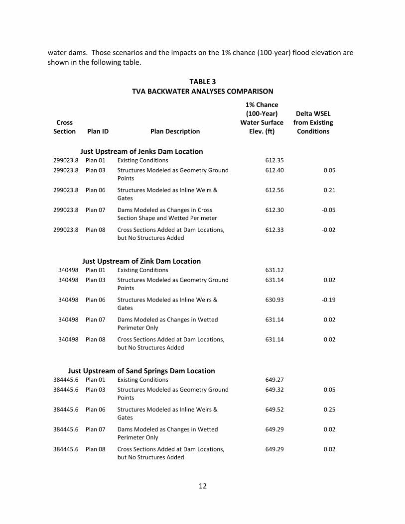
water dams. Those scenarios and the impacts on the 1% chance (100-year) flood elevation are shown in the following table.

TABLE 3 TVA BACKWATER ANALYSES COMPARISON

Cross Section Plan ID Plan Description

1% Chance (100-Year)

Water Surface Elev. (ft)

Delta WSEL from Existing

Conditions

Just Upstream of Jenks Dam Location 299023.8 Plan 01 Existing Conditions 612.35

299023.8 Plan 03 Structures Modeled as Geometry Ground Points

612.40 0.05

299023.8 Plan 06 Structures Modeled as Inline Weirs & Gates

612.56 0.21

299023.8 Plan 07 Dams Modeled as Changes in Cross Section Shape and Wetted Perimeter

612.30 -0.05

299023.8 Plan 08 Cross Sections Added at Dam Locations, but No Structures Added

612.33 -0.02

Just Upstream of Zink Dam Location 340498 Plan 01 Existing Conditions 631.12

340498 Plan 03 Structures Modeled as Geometry Ground Points

631.14 0.02

340498 Plan 06 Structures Modeled as Inline Weirs & Gates

630.93 -0.19

340498 Plan 07 Dams Modeled as Changes in Wetted Perimeter Only

631.14 0.02

340498 Plan 08 Cross Sections Added at Dam Locations, but No Structures Added

631.14 0.02

Just Upstream of Sand Springs Dam Location 384445.6 Plan 01 Existing Conditions 649.27

384445.6 Plan 03 Structures Modeled as Geometry Ground Points

649.32 0.05

384445.6 Plan 06 Structures Modeled as Inline Weirs & Gates

649.52 0.25

384445.6 Plan 07 Dams Modeled as Changes in Wetted Perimeter Only

649.29 0.02

384445.6 Plan 08 Cross Sections Added at Dam Locations, but No Structures Added

649.29 0.02

13

ALTERNATIVE SCENARIOS – UNSTEADY STATE HEC-RAS MODEL Several flow scenarios were analyzed using the HEC-RAS unsteady state backwater model furnished by the Corps of Engineers and further modified by Meshek. Table 4 lists those scenarios and their pertinent information. A full description of the various scenarios and the results are given in the following sections.

TABLE 4 UNSTEADY RAS MODELING SCENERIOS

SCENARIO NAME ARKANSAS RIVER FLOW (CFS)

COMMENTS

KEYS_900 900 cfs constant release made for Low Flow Requirements

No lateral inflow hydrographs added. Pilot Channel of 2’wide x 10’deep added for model stability. Channel “n” values modified to account for shallow flow depth

KEYS_3K 3,000 cfs constant release (one hydropower unit online at one half capacity)


KEYS_6K 6,000 cfs constant release (one hydropower unit online)


KEYS_12K_HYDPWR Hydropower releases of 12,000 cfs made at 2 specified intervals

No lateral inflow hydrographs added. Simulation of hydropower releases: One in the morning for 4 hours and one in the evening for 3 hours.

KEYS_12K_HYDP1WR Single 4 hour Hydropower releases of 12,000 cfs

No lateral inflow hydrographs added. Simulation of hydropower releases: One in the morning for 4 hours

KEYS_12K_INTERNALS 12, 000 constant release Hydropower Generation

Lateral tributary inflows added with no shift in hydrograph timing.

KEYS_12K_MOD_INTL 12, 000 constant release Hydropower Generation

Lateral tributary inflows added with a shift in hydrograph timing to coincide with river peaks.

KEYS_90K 90,000 peak release 10% Chance (10-year) flood

Peak flow of 90,000 cfs release from Keystone Dam using shape of Oct86 flood hydrograph – no lateral inflows added

KEYS_155K 155,000 peak release 2% Chance (50-year) flood


KEYS_205K 205,000 peak 1% Chance (100-year) flood


KEYS_300K 300,000 Keystone Dam release of Oct 86 flood


KEYS_350K 350,000 peak Levee design flood


14

SCENARIO – KEYS_900

A low flow simulation was made to simulate low flow conditions (minimum releases) from Keystone Dam to just below the proposed site of the Jenks low water dam. A constant release of 900 cfs from Keystone Dam was assumed and no lateral inflows from the intervening tributaries were added. Because the unsteady state backwater model tends to become unstable for very shallow flow conditions, a virtual pilot channel of 2’ wide by 10’ deep was added to the channel geometry. The additional 20 square feet of flow area at each cross section would not alter the conveyance capacity of the river to any significant degree. In addition to the pilot channel, additional cross sections were added at the proposed Sand Springs and Jenks low water dam locations that would better depict the change in hydraulic grade once the dams were actually designed. Finally, Manning’s “n” values were adjusted in the channel to reflect the shallow flow conditions and interpolated cross sections were added at two locations several miles downstream of the Jenks low water dam location where channel streambed grade changes were significant. The 900 cfs maximum water surface profile is shown on Panel 03P of Appendix C.

SCENARIO – KEYS_3K

A scenario of one hydropower unit running at one half capacity was evaluated, producing a constant flow of 3,000 cfs from Keystone Dam. No lateral inflows from the intervening tributaries were added. The same changes to the channel geometry as used in the KEYS_900 scenario were used in this analysis. The 3,000 cfs maximum water surface profile is shown on Panel 03P of Appendix C.


A scenario of one hydropower unit running at full capacity was evaluated, producing a constant flow of 6,000 cfs from Keystone Dam. No lateral inflows from the intervening tributaries were added. The same changes to the channel geometry as used in the KEYS-900a scenario were used in this analysis. The 6,000 cfs maximum water surface profile is shown on Panel 03P of Appendix C.

SCENARIO – KEYS_12K_HYDPWR

This alternative simulated a hydropower generation of 2 units generating for 4 hours in the morning and for 3 hours in the evening, a typical generation schedule. The same changes to the channel geometry as used in the KEYS_900 scenario were used in this analysis. The 12,000 cfs maximum water surface profile for this scenario is shown on Panel 03P of Appendix C.

15

SCENARIO – KEYS_12K_INTERNALS

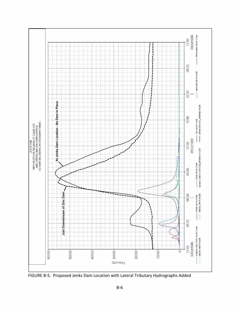
Between Keystone Dam and the proposed Jenks Dam location, 30 streams flow into the Arkansas River and drain approximately 140 square miles. Because of the significant intervening drainage area above the proposed and existing low water dam locations, analyses were performed to evaluate the effects of the lateral inflows coupled with a constant Keystone Dam release of 12,000 cfs (full hydropower generation release). Hydrographs developed in the previously mentioned HMS and HEC-1 models for a 1% chance (100-year frequency) flood event on each of the 30 tributary streams were added as lateral inflow hydrographs. No adjustments to the timing of the lateral inflow hydrographs were made. The hydrographs for the Arkansas River and the intervening tributaries at the 3 low water dam locations is shown on Figures B-1, B-3 and B-5 in Appendix B. The maximum water surface profile for this scenario is shown on Panel 03P of Appendix C.

SCENARIO – KEYS_12K_MOD_INTL This scenario is similar to the KEYS_12K_INTERNALS alternative, except that the lateral inflow hydrographs for the tributary basins have been shifted in time so that the tributary peak flows coincide with the Arkansas River hydrograph flood peak at the confluence with the tributaries. This would depict a “worst case scenario” for a normal hydropower release from Keystone Dam and a 100-year frequency flood occurring over the intervening basins down to the Jenks low water dam. The amount of time that each lateral tributary hydrograph was shifted is shown in Table 2. The resultant hydrographs for the Arkansas River and the intervening tributaries at the 3 low water dam locations are shown on Figures B-2, B-4 and B-6 in Appendix B. The maximum water surface profile for this scenario is shown on Panel 03P of Appendix C.


This scenario uses a 10% chance (10-year frequency) flood peak of 90,000 cfs established by the Corps of Engineers in the Tulsa County Watershed Study of 2002. The discharges developed in the 2002 study are for instantaneous flood peaks and no hydrographs for those floods were developed. Since the unsteady state model uses flood flow hydrographs as upstream boundary conditions, the October 1986 flood hydrograph was used to form the shape of the hydrograph. Values in the October 1986 hydrograph were multiplied by a factor of 0.3 to develop the 90,000 peak hydrograph. The maximum water surface profile for this scenario is shown on Panel 03P of Appendix C.



16




This scenario uses the releases from Keystone Dam that occurred during the October 1986 flood as the upstream boundary condition. The maximum water surface profile for this scenario is shown on Panel 03P of Appendix C.


This scenario uses a flood peak of 350,000 cfs (levee design flood for the Tulsa-West Tulsa and Jenks levees). The October 1986 flood hydrograph was used to form the shape of the 350,000 cfs hydrograph. Values in the October 1986 hydrograph were multiplied by a factor of 1.1667 to develop the 350,000 peak hydrograph. The maximum water surface profile for this scenario is shown on Panel 03P of Appendix C.

SCENARIO – KEYS_12K_HYDP1WR This scenario was developed to illustrate the travel time and attenuation of a typical hydrograph for a single hydropower generation of 12,000 cfs for 4 hours. It should be noted that the hydrograph peak takes around 5 hours to travel from Keystone Dam to the Sand Springs proposed dam location, about 4 hours to travel from the Sand Springs dam location to the Zink Dam location, and another 4.5 hours to travel from the Zink Dam to the proposed Jenks Dam location. The peak flow attenuates from 12, 000 just below Keystone Dam to 10,450 cfs at the Sand Springs Dam, to 8,690 cfs at the Zink Dam, and then to 7,730 cfs at the Jenks Dam location. The travel times and attenuations do not consider the proposed Sand Springs and Jenks low water dams being in place with their proposed operational procedures. Figure B-7 in Appendix B illustrates the hydrograph travel and attenuation for the 12,000 cfs hydropower release.

17

ALTERNATIVE SCENARIOS –STEADY STATE HEC-RAS MODEL Several different scenarios were evaluated using the modified Corps of Engineers’ steady state

backwater model for the Arkansas River. The primary focus of the evaluations was to

determine the amount of rise in water surface elevations for various flows, including the 1%

chance (100-year frequency) flood of 205,000 cfs and the levee design flood of 350,000 cfs.

Each scenario was compared to the existing conditions backwater model at each cross section.

Since no final design exists for any of the proposed or modified low water dams, the structures

were evaluated using simplified designs. There were 4 basic ways of evaluating the low water

dams: 1) Existing Conditions with the existing Zink Dam in place and no low water dams at the

Sand Springs or Jenks locations. 2) Model each low water dam as a bridge using piers to

simulate the structure as if all gages are open. This technique would give the least amount of

rise in water surface elevations. 3) Model the low water dams with a combination of bridge

piers and blocked obstructions. The blocked obstructions would represent the area block by

the weir at the low water dams. 4) Model each structure using the Inline Structure Option in

the HEC-RAS program. This option allows the input of actual weirs and gates and gives the

option to have different gate opening scenarios. Table 5 gives the amounts of rise at key

locations for the 4 different scenarios evaluated. Profiles of the 4 scenarios are shown in

Appendix C on Panel 04P. It should be noted that the calculated water surface elevations for

the final designs could be higher by 0.1 to 0.5 feet based on using a stepped overflow structure

instead of an Ogee Weir and adding roughened channel sluices for fish passage and

recreational venues. An examination of the changes in floodplain areas for the various plans

indicates the 1% chance (100-year) floodplain will increase in area by about 200 acres (1%) over

the entire length of the project area.

18

TABLE 5

COMPUTED WATER SURFACE ELEVATIONS PLAN COMPARISONS1

LOCATION AND CROSS SECTION NUMBER

EXISTING CONDITIONS – EXISTING ZINK DAM IN, NO DAMS AT JENKS OR SAND SPRINGS ELEV

EXISTING CONDITIONS WITH JENKS RIVER DISTRICT IN AS PLANNED ELEV/RISE FT.

PLAN A – LOW WATER DAMS MODELED ONLY AS BRIDGE PIERS ELEV/ RISE FT.2

PLAN A1 - LOW WATER DAMS MODELED AS BRIDGE PIERS WITH BLOCKED AREAS AS WEIRS ELEV/ RISE FT.2

PLAN A1-2 - LOW WATER DAMS MODELED AS INLINE STRUCTURES ELEV/ RISE FT.2

1% Chance (100-year) flood (205,000 cfs)

Above Jenks LWD – 298676.5

612.23 612.67 / 0.44 612.69 / 0.02 612.78 / 0.11 612.78 / 0.11

Above Zink LWD – 340498.0

631.11 631.12 / 0.01 630.78 / -0.34 630.79 / -0.33 630.74 / -0.38

Above Sand Springs LWD – 384445.6

649.29 649.29 / 0.00 649.31 / 0.02 649.65 / 0.36 649.44 / 0.15

Levee Design Flood (350,000 cfs)


618.11 619.5 / 1.39 618.77 / -0.73 619.62 / 0.12 618.88 / -0.62


638.00 638.11 / 0.11 637.95 / -0.16 638.03 / -0.08 637.89 / -0.22


657.44 657.44 / 0.00 657.52 / 0.08 657.76 / 0.32 657.49 / 0.05

1 Plans A, A1, and A1-2 all assume the Jenks River District development is in as planned by Jenks.

2 For Jenks Dam Area, Rise is the increase above the “Existing Conditions plus Jenks River District Development In

Place as Proposed” condition.

19

River District Development

The proposed River District development is a 424-acre, multi-use project planned for the west bank of the Arkansas River south of the Creek Turnpike near Jenks, Oklahoma . This development consists of “moving” the existing right bank of the Arkansas River eastward and filling in the existing floodplain to elevation 617.0 feet, N.G.V.D. The proposed Jenks low water dam would tie into the River District development near cross section 295373.8. Figure 5 shows the approximate location of the proposed River District development, and Figures 6 and 7 show the extent of the proposed River District fill for 2 cross section locations.

20

FIGURE 6. RIVER DISTRICT DEVELOPMENT AT CROSS SECTION 295373.8

FIGURE 7. RIVER DISTRICT DEVELOPMENT AT CROSS SECTION 297137.5

21

“NO RISE” ALTERNATIVE AND RECOMMENDED PLAN

No Rise Alternative

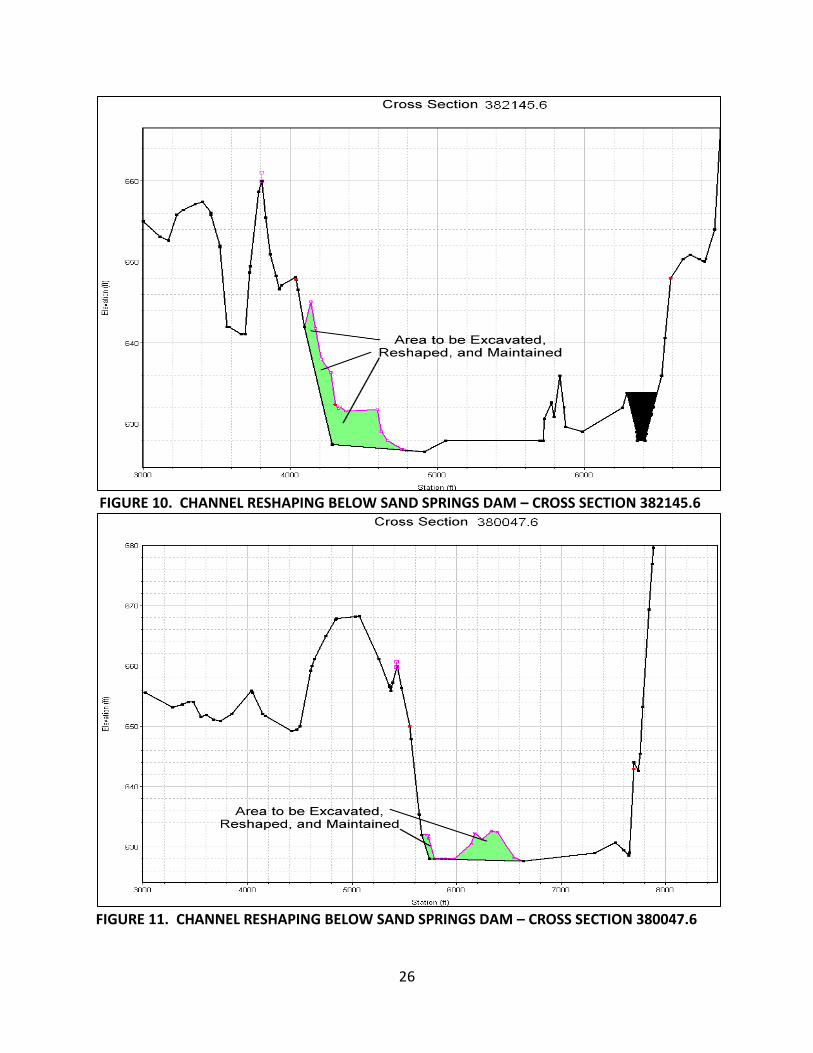
Since all of the alternatives presented in Table 5 produce a rise above the 1% chance (100-year) flood at the Jenks and Sand Springs locations, an additional alternative was included for analysis that would minimize or eliminate the water surface rise. In this scenario, the proposed Jenks low water dam would moved about 2,000 feet north and placed along an alignment near cross section 297137.5 as depicted in Figure 8. This alignment could tie into either the existing high ground on the west end or to the proposed Jenks River District development fill, if constructed. The Jenks low water dam would consist of weirs located on either side of a gated structure. The weirs would be 500-600 feet in length with crests at elevation 598.0. With a weir crest elevation of 598 instead of the previous 596, the static pool would be 2 foot deeper and would extend closer to development located on the east side of the river north of the 96th Street bridge. The gated structure would consist of 7 - 100’ wide gates able to drop to streambed level. This alignment and configuration would produce a net decrease in the 1% chance and Levee Design Floods upstream of the Jenks low water dam. Table 6 gives elevation information regarding this alternative. For the Zink low water dam, no additional revisions are necessary since adding gates to the existing low water dam where none now exist will produce a net decrease in the 1% chance (100-year) and Levee Design Floods. The dam would consist of weirs located on either side of a gated structure at crest elevation 620.0. The gated structure would be comprised of 6 – 100’ wide gates able to be dropped to streambed level. Refer to Table 6 for elevation information. At the Sand Springs low water dam location, it was discovered that reshaping and maintaining the left (north) portion of the existing river channel downstream of the proposed dam alignment and for a distance of about 2,400 feet will result in lower tailwater conditions and thus an overall decrease in the 1% chance (100-year) and Levee Design Floods for all scenarios. The dam would consist of weirs located on either side of a gated structure at crest elevation 638.0. The gated structure would be comprised of 9 – 100’ wide gates able to be dropped to streambed level. Figures 9 through 11 illustrate this configuration. Table 6 gives the elevation data for this scenario. Since there is not yet a specific design proposed for the actual weir construction, a weir coefficient for the overflow sections of the 3 low water dams was not available. Therefore, a weir coefficient of 3.1 was used in the weir flow equations. Any decrease in the selected weir flow coefficients will ultimately cause an increase in computed water surface elevations without offsetting geometry or structural changes.

22

Recommended Plan

The plan recommended in this report consists of the No Rise scenarios for the Jenks and Zink Dams, but no channel shaping below the Sand Springs Dam due to the sensitive environmental nature of that option. In addition, the weir sections at each dam would consist of a stepped weir deck below each structure to prevent any roller effect typical of an Ogee type weir. All gates would be Obermeyer gates. The Jenks low water dam would be located near section 297137.5, but could be shifted slightly further north or south to accommodate construction requirements and needs. The weir crest would be at elevation 596 and the gated structure would consist of 7 – 100’ wide x 6’ high gates with sills placed at elevation 590.0. The existing Zink low water dam would modified at its current location. The weir crest would be raised from it current elevation of 617.0 to an elevation of 620.0 to increase depth. The gated structure would consist of 6 – 100’ wide x 8.5’ high gates with sills placed at elevation 611.5. The Sand Springs low water dam would have a weir crest at elevation 638.0 and would consist of a gated structure with 8 – 100’ wide x 10’ high gates. Gate sills would be at elevation 628.0. No channel shaping would be required.

24

TABLE 6 COMPUTED WATER SURFACE ELEVATIONS

“NO RISE” ALTERNATIVE & RECOMMENDED PLAN LOCATION AND CROSS SECTION NUMBER

EXISTING CONDITIONS – EXISTING ZINK DAM IN, NO DAMS AT JENKS OR SAND SPRINGS ELEV

“No Rise” ALTERNATIVE - JENKS DAM RELOCATED, ZINK DAM MODIFIED, CHANNEL SHAPING DOWNSTREAM OFSAND SPRINGS DAM ELEV/ RISE FT.

RECOMMENDED PLAN – JENKS DAM RELOCATED, ZINK DAM MODIFIED, NO

CHANNEL SHAPING DOWNSTREAM OF SAND

SPRINGS DAM ELEV / RISE FT.

1% Chance (100-year) flood (205,000 cfs)


612.23 611.77 /- 0.46 611.86 / -0.37


631.11 630.84 / -0.27 631.00 / -0.11


649.29 649.27 / -0.02 649.48 / 0.19

Levee Design Flood (350,000 cfs)


618.11 617.61 / -0.50 617.74 / -0.37


638.00 637.92 / -0.08 638.24 / 0.24


657.44 657.47 / 0.03 657.64 / 0.20

26

FIGURE 10. CHANNEL RESHAPING BELOW SAND SPRINGS DAM – CROSS SECTION 382145.6

FIGURE 11. CHANNEL RESHAPING BELOW SAND SPRINGS DAM – CROSS SECTION 380047.6

27

FLOW FREQUENCY AND DURATION ANALYSES

One of the most important factors in the design and operational evaluation of the existing and

proposed low water dams is the duration and frequency of Arkansas River flows for various

discharge values and for varying operational scenarios. Critical factors such as seasonal fish

migrations, recreational venues and scheduled times, seasonal fish spawning, and water quality

requirements all play an important role in the design and operation of the dams. It should be

noted that Keystone Dam is equipped with two hydropower generating units, each of which

discharges approximately 6,000 cfs at full operation for a total discharge of 12,000 cfs from the

dam. The electricity generated from these units is part of the Southwestern Power

Administration’s (SWPA) electrical grid system and are for peak loads only. During the summer

a typical schedule for operation of the hydropower units involves peak generation for a period

of 4-5 hours in the evening (1 p.m. through 6 p.m.) on a Monday through Friday basis. During

the winter months, the operation involves peak generation for 2 periods during the day: 5 a.m.

through 10 a.m. and 5 p.m. through 10 p.m., also on a Monday through Friday basis. These

times and schedules are variable depending on SWPA’s customers’ needs and demands.

A peak discharge frequency curve for the Keystone Dam releases was previously developed by

the Tulsa District Corps of Engineers and has been presented in this report as Figure 5.

However, of equal importance to the design and operation of the project are the daily and

hourly flow durations for flows in the range of 100 to 12,000 cfs. Mean daily flow records are

available from the US Geological Survey for the Arkansas River at the 11th Street gage for the

period June 24, 1964 through the current date. Hourly flow data is also available from the

USGS for the period October 11th, 1987 through September 30th, 2008.

Table 7 presents mean monthly flow values determined from daily averages as recorded at the

11th Street stream gage on the Arkansas River for the period October 1964 through September

2008. The values highlighted in blue represent months where the monthly mean is above a

flow of 15,000 cfs, which represents those values in the upper flow range. The values

highlighted in pink represent months where the flows average below 1,000 cfs and represent

flows occurring in the lower range. The months with no color highlighting are for those flows in

the intermediate range. As illustrated in the table, the fall and winter months are more likely to

experience periods of low flows while the spring and summer months are more likely to

experience periods of flows exceeding 15,000 cfs.

28

TABLE 7 ARKANSAS RIVER AT 11TH ST. GAGE

MEAN MONTHLY FLOWS

Jan Feb Mar Apr May Jun Jul Aug Sep Oct Nov Dec

1964 490.6 19,340 8,100

1965 4,043 674.2 1,790 7,130 5,824 22,450 10,710 2,443 18,680 3,498 2,484 2,985

1966 2,056 4,571 2,860 1,775 2,733 2,595 1,740 1,821 2,313 2,331 1,318 738.6

1967 483.3 494.1 1,400 692.9 880.9 5,350 16,470 5,712 4,847 5,795 1,614 1,148

1968 1,760 2,214 3,896 7,101 8,653 8,686 3,049 6,070 4,574 5,541 5,314 6,085

1969 3,336 3,696 8,355 10,960 25,950 20,770 7,345 3,404 8,011 4,599 3,002 2,740

1970 2,598 2,331 1,399 19,470 9,448 7,498 6,968 1,332 1,219 2,432 2,589 1,611

1971 1,466 1,597 4,045 2,034 2,441 6,714 3,463 2,979 4,326 3,154 4,816 5,955

1972 3,711 1,924 1,517 1,522 2,858 2,664 2,884 1,949 2,163 1,644 3,423 3,013

1973 12,260 13,640 37,350 44,460 26,890 7,660 3,361 4,569 4,793 48,920 11,640 12,260

1974 9,822 10,380 24,530 10,960 17,490 19,630 6,789 4,912 11,390 5,113 39,390 8,569

1975 11,010 18,550 17,520 11,450 21,090 38,930 8,808 4,364 3,546 1,745 2,052 1,661

1976 2,009 1,940 2,083 3,700 8,413 6,908 9,242 3,275 1,301 1,203 1,391 1,124

1977 1,155 518.2 490.2 700.6 8,881 15,550 8,789 6,778 12,920 4,393 4,990 1,894

1978 2,833 4,359 8,392 6,273 8,191 13,230 4,691 2,088 1,866 765.8 1,548 1,891

1979 1,409 2,301 13,870 15,180 11,900 8,542 6,822 6,856 7,401 1,388 18,940 7,211

1980 5,333 4,897 6,335 18,770 19,190 14,420 7,728 1,129 1,697 517.2 567.5 659.2

1981 780.2 712.5 668.4 556.6 2,583 5,712 3,867 2,534 3,082 1,755 11,490 3,935

1982 1,597 4,992 7,302 2,601 24,560 31,810 16,000 5,232 1,577 836.4 457.4 582

1983 2,254 3,853 6,566 29,190 18,610 13,410 12,270 1,409 1,293 5,571 3,977 2,108

1984 1,417 3,160 16,350 35,800 12,880 8,744 5,059 2,631 1,988 836 867.7 5,182

1985 8,464 6,252 21,000 10,630 14,500 13,180 7,063 4,282 6,695 26,600 10,460 11,690

1986 7,029 3,773 3,947 5,115 11,520 10,560 7,912 3,612 3,464 72,720 23,230 11,270

1987 9,578 19,450 42,890 18,970 14,000 28,880 19,450 6,210 6,684 7,070 2,067 5,335

1988 14,940 7,628 19,520 29,190 7,841 3,135 2,920 1,665 3,228 2,089 1,770 2,141

1989 2,747 2,308 3,736 5,791 4,485 16,750 11,080 10,750 23,280 7,313 3,510 1,818

1990 5,262 5,234 21,040 22,550 12,380 7,085 4,690 2,102 1,577 739.1 922 659.5

1991 1,279 1,460 662.3 2,179 4,302 4,572 1,314 1,150 2,585 2,165 3,112 6,805

1992 5,767 2,931 2,925 3,151 3,110 13,470 13,150 16,190 7,384 989.6 9,114 16,830

1993 19,630 22,500 18,110 16,640 81,400 32,010 24,800 16,690 7,753 2,771 2,731 1,985

1994 2,779 3,598 4,704 12,510 23,970 6,138 2,820 3,208 1,156 858 6,489 6,596

1995 3,646 2,132 13,540 5,994 25,960 69,820 27,790 32,970 5,573 3,024 2,206 2,730

1996 2,953 4,236 2,011 1,141 1,871 4,726 2,712 9,620 10,410 11,720 17,080 11,950

1997 5,191 9,221 11,390 25,360 12,580 11,250 24,650 17,630 12,590 11,730 4,093 6,554

1998 19,850 9,726 25,000 28,580 17,390 6,306 4,549 1,726 892.8 18,270 54,540 10,430

1999 5,245 15,920 20,520 22,650 34,310 42,850 37,630 8,196 4,955 3,649 1,353 13,380

2000 6,298 4,274 26,650 18,840 10,680 8,933 14,810 4,073 2,429 2,048 6,672 3,036

2001 4,225 10,400 24,620 7,247 9,956 17,730 5,194 783 1,078 1,765 1,340 545.1

2002 869.5 3,283 1,388 2,365 4,273 12,520 8,209 5,166 4,026 15,010 7,116 3,122

2003 3,482 3,807 15,970 10,090 11,700 10,990 4,527 2,677 5,513 11,360 2,429 1,914

2004 2,821 7,036 29,200 9,540 15,310 10,370 18,210 8,966 2,010 1,661 6,984 4,924

2005 12,220 10,730 8,418 5,793 3,554 27,240 8,908 11,900 7,013 3,065 2,196 955

2006 1,124 1,884 840.9 872.7 8,300 1,633 2,802 2,085 1,300 305 58.8 84.8

2007 163.4 1,314 5,749 25,440 30,470 44,040 52,540 20,280 7,636 6,372 2,329 3,023

2008 4,189 9,498 9,664 17,020 29,400 40,010 21,960 4,623 21,110

Mean

YEAR

Monthly mean in cfs (Calculation Period: 1964-10-01 -> 2008-09-30)

Period-of-record for statistical calculation restricted by user

4,710

** No Incomplete data have been used for statistical calculation

16,000 10,800 6,090 5,670 7,180 7,1105,020 5,800 11,400 12,200 14,400

29

To gain a more detailed picture of the periods of high and low discharges, flow duration curves

were developed. Figures D-1 and D-2 in Appendix D show plots of the mean monthly and mean

daily flows on the Arkansas River at the 11th Street gage, respectively. Additionally, mean

monthly and mean hourly flow duration curves have been developed and are shown in Figures

D-3 and D-4 in Appendix D. The information show in the hourly flow duration curve is

summarized in Table 8.

TABLE 8 ARKANSAS RIVER AT 11TH ST. GAGE

HOURLY FLOW EXCEEDENCE

MONTH OR TIMEFRAME FLOW, C.F.S. PERCENT OF TIME FLOW IS EQUALED OR EXCEDDED

Yearly 1,000 78%

March through May 1,000 85%

May through September 1,000 81%

May 1,000 87%

June 1,000 88%

July 1,000 85%

August 1,000 76%

September 1,000 68%

30

RECOMMENDATIONS FOR ADDITIONAL

HYDROLOGIC AND HYDRAULIC ANALYSES The information provided in this Technical Memorandum (excluding the existing conditions

Arkansas River backwater analyses) should be considered exploratory and conceptual in nature.

Additional detailed hydrologic and hydraulic analyses will be required to develop the final

design, placement, and operation of the proposed low water dams. The following is a

discussion of the required analyses.

FIELD SURVEYS To ensure adequate levee freeboard is maintained, surveys along the crown of the levees

should be performed at the beginning of the next phase of work. Additionally, detailed surveys

of the channel and overbanks along the alignment of the proposed dam locations will be

required for design of the structures.

HYDROLOGIC ANALYSES

The frequency peak flow information previously developed for the Arkansas River by the Corps

of Engineers in 2002 will continue to be used for the backwater impact analyses of the low

water dams. However, since that data is for instantaneous discharges only and the future

hydraulic analyses will be unsteady state in nature, a hydrograph depicting the flow of the river

will be required. One possible scenario is to use the October 1986 flood hydrograph occurring

just below Keystone Dam as a general shape and configuration for the frequency releases, just

altering the magnitude of the hydrograph.

In addition to the Arkansas River hydrology, the hydrology information developed in this

Technical Memorandum for the intervening drainage basins should be reviewed and confirmed

for use in the operational requirements of the low water dams.

STEADY STATE BACKWATER ANALYSES

A final “With Project Conditions” backwater profile and floodway model that includes the final

plan for the proposed and modified low water dams will be required for submittal to FEMA.

The final selected low water dam gate and weir structure configuration will need to be input

into the final models.

UNSTEADY STATE BACKWATER ANALYSES WITH OPERATIONAL REQUIREMENTS

In order to properly design the low water dam structures and their operational requirements,

an unsteady state backwater model, such as HEC-RAS version 4.0 or MIKE21 will be needed.

Either of these models will allow the modeling of river flows over time. The modeling will allow

31

the determination of the actual number of gates to be installed at each structure and the

number and amount of gate openings at each structure for given operational scenarios.

A-1

APPENDIX A

ARKANSAS RIVER CORRIDOR STUDY MASTER PLAN H&H ANALYSES VERIFICATION PLOTS

A-2

FIGURE A-1 OCT 1986 FLOW HYDROGRAPH VERIFICATION

FIGURE A-2 OCT 1986 STAGE HYDROGRAPH VERIFICATION

A-3

FIGURE A-3 AUG 2008 FLOW HYDROGRAPH VERIFICATION

FIGURE A-4 AUG 2008 STAGE HYDROGRAPH VERIFICATION

A-4

FIGURE A-5 SEP 2008 FLOW HYDROGRAPH VERIFICATION

FIGURE A-6 SEP 2008 STAGE HYDROGRAPH VERIFICATION

A-5

FIGURE A-7 OCT 2008 FLOW HYDROGRAPH VERIFICATION

FIGURE A-8 OCT 2008 STAGE HYDROGRAPH VERIFICATION

A-6

FIGURE A-9 MAY 2009 FLOW HYDROGRAPH VERIFICATION

FIGURE A-10 MAY 2009 FLOW HYDROGRAPH VERIFICATION

B-1

APPENDIX B

ARKANSAS RIVER CORRIDOR STUDY MASTER PLAN H&H ANALYSES FLOW HYDROGRAPHS FOR STUDY SCENARIOS

B-2

FIGURE B-1. Proposed Sand Springs Dam Location with Lateral Tributary Hydrographs Added

B-3

FIGURE B-2. Proposed Sand Springs Dam Location with Lateral Tributary Hydrographs Shifted

B-4

FIGURE B-3. Existing Zink Dam Location with Lateral Tributary Hydrographs Added

B-5

FIGURE B-4. Existing Zink Dam Location with Lateral Tributary Hydrographs Shifted

B-6

FIGURE B-5. Proposed Jenks Dam Location with Lateral Tributary Hydrographs Added

B-7

FIGURE B-6. Proposed Jenks Dam Location with Lateral Tributary Hydrographs Shifted

B-8

FIGURE B-7. Hydrograph Travel Time and Attenuation

C-1

APPENDIX C

ARKANSAS RIVER CORRIDOR STUDY MASTER PLAN H&H ANALYSES STEADY STATE AND UNSTEADY STATE BACKWATER PROFILES

01P

ARKA

NSAS

RIVE

R CO

RRID

ORMA

STER

PLAN

(TULS

A CO.

)

FLOO

D PR

OFILE

S - D

UPLIC

ATE E

FFEC

TIVE M

ODEL

ARKA

NSAS

RIVE

R

Old H

wy 10

4St

ate H

wy 10

4

State

Hwy

72

US H

wy 64

(Mem

orial

Rd)

02P

ARKA

NSAS

RIVE

R CO

RRID

ORMA

STER

PLAN

(TULS

A CO.

)

FLOO

D PR

OFILE

S - D

UPLIC

ATE E

FFEC

TIVE M

ODEL

ARKA

NSAS

RIVE

R

Railro

ad B

ridge

Hwy 9

7

11th

St. B

ridge

s23

rd St

. Brid

ge

I - 24

4 Brid

ge

Pede

strian

Brid

ge

Keys

tone

Dam

I - 44

Brid

ge

71st

St. B

ridge

96th

St. B

ridge

Cree

k Tpk

03P

ARKA

NSAS

RIVE

R CO

RRID

ORMA

STER

PLAN

(TULS

A CO.

)

FLOO

D PR

OFILE

S - U

NSTE

ADY F

LOW

MODE

L

ARKA

NSAS

RIVE

R

Railro

ad B

ridge

Hwy 9

7

11th

St. B

ridge

s23

rd St

. Brid

ge

I - 24

4 Brid

ge

Pede

strian

Brid

geEx

isting

Zinc

Dam

Prop

osed

Sand

Spr

ings D

am

Keys

tone

Dam

I - 44

Brid

ge

71st

St. B

ridge

96th

St. B

ridge

Cree

k Tpk

Prop

osed

Jenk

s Dam

04P

ARKA

NSAS

RIVE

R CO

RRID

ORMA

STER

PLAN

(TULS

A CO.

)

FLOO

D PR

OFILE

S - C

OMPA

RISO

N OF

PLAN

S

ARKA

NSAS

RIVE

R

Railro

ad B

ridge

Hwy 9

7

11th

St. B

ridge

s23

rd St

. Brid

ge

I - 24

4 Brid

ge

Pede

strian

Brid

ge

Keys

tone

Dam

I - 44

Brid

ge

71st

St. B

ridge

96th

St. B

ridge

Cree

k Tpk

Sand

Spr

ings

Low

Water

Dam

Zink L

ow

Water

Dam

Jenk

s-Sou

th Tu

lsaLo

w Wa

ter D

am

APPENDIX D

ARKANSAS RIVER CORRIDOR STUDY MASTER PLAN H&H ANALYSES FLOW FREQUENCY AND DURATION

FIGURE D-1. Arkansas River, 11th Street Gage, Mean Monthly Flows

FIGURE D-2. Arkansas River, 11th Street Gage, Mean Daily flows

FIGURE D-3. Arkansas River, 11th Street Gage, Mean Monthly Flow Duration Curve

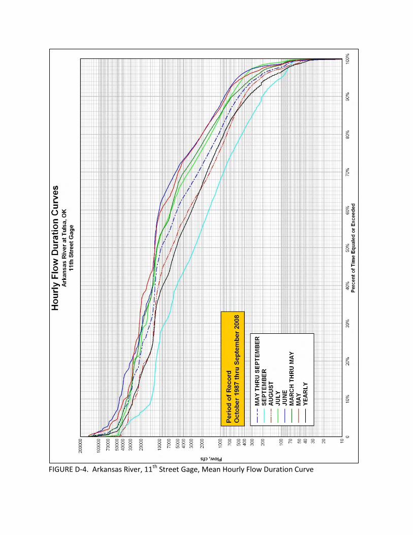
FIGURE D-4. Arkansas River, 11th Street Gage, Mean Hourly Flow Duration Curve

ARKANSAS RIVER CORRIDOR STUDY MASTER...

Documents

Transcript of ARKANSAS RIVER CORRIDOR STUDY MASTER...