Arithmetic of del Pezzo surfaces of degree 1 - Rice...

Arithmetic of del Pezzo surfaces of degree 1

by

Anthony Varilly-Alvarado

A.B. (Harvard University) 2003

A dissertation submitted in partial satisfaction of the

requirements for the degree of

Doctor of Philosophy

in

Mathematics

in the

GRADUATE DIVISION

of the

UNIVERSITY OF CALIFORNIA, BERKELEY

Committee in charge:Professor Bjorn Poonen, Chair

Professor Paul VojtaProfessor Robert Littlejohn

Spring 2009

The dissertation of Anthony Varilly-Alvarado is approved:

Chair Date

Date

Date

University of California, Berkeley

Spring 2009


Copyright 2009

by


1

Abstract


by


Doctor of Philosophy in Mathematics

University of California, Berkeley

Professor Bjorn Poonen, Chair

We study the density of rational points on del Pezzo surfaces of degree 1 for the Zariski

topology and the adelic topology. For a large class of these surfaces over Q, we show that the

set of rational points is dense for the Zariski topology. We achieve our results by carefully

studying variations of root numbers among the fibers of elliptic surfaces associated to del

Pezzo surfaces of degree 1. Our results in this direction are conditional on the finiteness of

Tate-Shafarevich groups for elliptic curves over Q.

We also explicitly study the Galois action on the geometric Picard group of del

Pezzo surfaces of degree 1 of the form

w2 = z3 +Ax6 +By6

in the weighted projective space Pk(1, 1, 2, 3), where k is a global field of characteristic

not 2 or 3 and A,B ∈ k∗. Over a number field, we exhibit an infinite family of minimal

surfaces for which the rational points are not dense for the adelic topology; i.e., minimal

surfaces that fail to satisfy weak approximation. These counterexamples are explained by

a Brauer-Manin obstruction.

Professor Bjorn PoonenDissertation Committee Chair

i

To my father

ii

Contents

1 Motivation and main results 11.1 Guiding questions in diophantine geometry . . . . . . . . . . . . . . . . . . 11.2 Birational invariance and a theorem of Iskovskikh . . . . . . . . . . . . . . . 31.3 Del Pezzo surfaces and rational conic bundles . . . . . . . . . . . . . . . . . 41.4 Survey of arithmetic results . . . . . . . . . . . . . . . . . . . . . . . . . . . 61.5 Del Pezzo surfaces of degree 1: Main results . . . . . . . . . . . . . . . . . . 10

1.5.1 Zariski density of rational points . . . . . . . . . . . . . . . . . . . . 111.5.2 Weak approximation . . . . . . . . . . . . . . . . . . . . . . . . . . . 13

2 Background material 162.1 Del Pezzo surfaces are separably split . . . . . . . . . . . . . . . . . . . . . 162.2 Further properties of del Pezzo surfaces . . . . . . . . . . . . . . . . . . . . 18

2.2.1 The Picard group . . . . . . . . . . . . . . . . . . . . . . . . . . . . . 182.2.2 Galois action on the Picard group . . . . . . . . . . . . . . . . . . . 192.2.3 Anticanonical models . . . . . . . . . . . . . . . . . . . . . . . . . . 192.2.4 Del Pezzo surfaces of degree 1 and elliptic surfaces . . . . . . . . . . 21

2.3 Brauer-Manin obstructions . . . . . . . . . . . . . . . . . . . . . . . . . . . 222.3.1 The Brauer group of a scheme . . . . . . . . . . . . . . . . . . . . . 232.3.2 The Brauer-Manin set . . . . . . . . . . . . . . . . . . . . . . . . . . 242.3.3 Conjectures of Colliot-Thelene and Sansuc . . . . . . . . . . . . . . . 252.3.4 The Hochschild-Serre spectral sequence in etale cohomology . . . . . 262.3.5 Galois descent of line bundles . . . . . . . . . . . . . . . . . . . . . . 28

3 Zariski density of rational points on del Pezzo surfaces of degree 1 303.1 Root numbers and flipping . . . . . . . . . . . . . . . . . . . . . . . . . . . . 31

3.1.1 The root number of Eα/Q : y2 = x3 + α . . . . . . . . . . . . . . . . 323.1.2 The root number of Eα/Q : y2 = x3 + αx . . . . . . . . . . . . . . . 36

3.2 The Modified Square-free Sieve . . . . . . . . . . . . . . . . . . . . . . . . . 383.2.1 Making sure that C does not vanish . . . . . . . . . . . . . . . . . . 423.2.2 An application of the modified sieve . . . . . . . . . . . . . . . . . . 42

3.3 Proof of Theorems 1.5.3 and 1.5.4 . . . . . . . . . . . . . . . . . . . . . . . 443.4 Diagonal del Pezzo surfaces of degree 1 . . . . . . . . . . . . . . . . . . . . . 483.5 Towards weak-weak approximation . . . . . . . . . . . . . . . . . . . . . . . 52

iii

4 Weak approximation on del Pezzo surfaces of degree 1 564.1 Exceptional curves on del Pezzo surfaces of degree 1 . . . . . . . . . . . . . 56

4.1.1 The Bertini involution . . . . . . . . . . . . . . . . . . . . . . . . . . 564.1.2 The bianticanonical map . . . . . . . . . . . . . . . . . . . . . . . . . 574.1.3 Proof of Theorem 1.5.9 . . . . . . . . . . . . . . . . . . . . . . . . . 58

4.2 Exceptional curves on diagonal surfaces . . . . . . . . . . . . . . . . . . . . 604.3 Galois action on PicXK . . . . . . . . . . . . . . . . . . . . . . . . . . . . . 64

4.3.1 An observation . . . . . . . . . . . . . . . . . . . . . . . . . . . . . . 664.4 Finding cyclic algebras in BrX . . . . . . . . . . . . . . . . . . . . . . . . . 68

4.4.1 Review of cyclic algebras . . . . . . . . . . . . . . . . . . . . . . . . 684.4.2 Cyclic Azumaya algebras . . . . . . . . . . . . . . . . . . . . . . . . 694.4.3 Cyclic algebras on rational surfaces . . . . . . . . . . . . . . . . . . . 70

4.5 Counterexamples to Weak Approximation . . . . . . . . . . . . . . . . . . . 714.5.1 A warm-up example . . . . . . . . . . . . . . . . . . . . . . . . . . . 714.5.2 Main Counterexamples . . . . . . . . . . . . . . . . . . . . . . . . . . 73

iv

Acknowledgments

It is a pleasure to thank the people whose support throughout my years in graduate school

made this thesis possible. First, I thank Bjorn Poonen. He has profoundly influenced my

development as a mathematician; his passion, intuition, creativity, patience, work ethic and

generosity are constant sources of inspiration for me. His careful reading of earlier drafts

of this thesis made it a genuinely better document. I also thank Paul Vojta for his careful

reading of this thesis.

During my graduate education, I benefitted greatly from the insights, questions,

lectures, advice and help of Jean-Louis Colliot-Thelene, David Harari, Andrew Kresch,

Ronald van Luijk, Martin Olsson, Ken Ribet, Bernd Sturmfels, and Peter Teichner.

Jean-Louis Colliot-Thelene, Samir Siksek, Michael Stoll and especially Ronald van

Luijk afforded me wonderful opportunities to disseminate the contents of this thesis.

Pat Barrow, David Brown, Dan Erman and Bianca Viray made my years in Evans

Hall tremendously enjoyable. Their friendship and support through the journey of graduate

school have greatly shaped me and my views of mathematics. In this vein, I also want to

thank my fellow graduate students Anton Geraschenko, Radu Mihaescu, David Penneys,

Cecilia Salgado, Chris Schommer-Pries, David Smyth, and David Zywina. I thank my fellow

housemates at Fulton Manor for an ideal atmosphere at home.

I learnt a great deal of mathematics from my collaborators Dan Erman, Damiano

Testa, Mauricio Velasco and David Zywina. Working together was a real pleasure.

Part of the research of this thesis was carried out while I enjoyed the hospitality

of the Equipe de Geometrie Algebrique at the Universite de Rennes 1 in 2007. I thank

Laurent Moret-Bailly and Rob de Jeu for all their help during my stay there, as well as

Sylvain Brochard and Jerome Poineau for making the experience memorable.

The staff in the Evans Hall, particularly Barbara Peavy, Marsha Snow and Barb

Waller, created a superb working environment. Thank you.

Finally, I thank my family. To my father, who first showed me beauty in Mathe-

matics, I owe my passion for the subject. I continually endeavor to mirror my late mother’s

strong spirit and selflessness (I miss you every day). I have learned much from my younger

brother Patrick, whose example in many ways I try to follow. I also thank Paola and Mima

for their love and support. Finally, I thank Sarah, my partner in life, from the bottom of

my heart, for her love and encouragement in our continuing journey.

1

Chapter 1

Motivation and main results

1.1 Guiding questions in diophantine geometry

Let k be a global field, i.e., a finite extension of Q or Fp(t) for some prime p, let

Ak denote its ring of adeles, and let X be a smooth projective geometrically integral variety

over k. Generally speaking, diophantine geometers seek to “describe” the set X(k) of k-

rational points of X. For example, we are interested in determining whether X(k) is empty

or not. If X(k) 6= ∅, then we may further want to know something about the qualitative

nature of X(k): is it dense for the Zariski topology of X? Is the image of the natural

embedding X(k) → X(Ak) dense for the adelic topology? If not, can we account for the

paucity of k-rational points? We may also pursue a more quantitative study of X(k). For

instance, we might try to prove asymptotic formulas for the number of k-points of bounded

height on some special Zariski-open subset of X.

On the other hand, if X(k) = ∅, then we might try to account for the absence

of k-rational points. For example, the existence of embeddings X(k) → X(kv) for every

completion kv of k shows that a necessary condition for X to have a k-rational point is

X(kv) 6= ∅ for all completions kv of k. (1.1)

To illustrate this, note that the projective plane conic x2+y2 = 3z2 over Q has no Q3-points,

and hence it contains no Q-points.

We say that X is locally soluble whenever (1.1) is satisfied, and we note that local

solubility makes sense for any variety over a global field. Whenever checking (1.1) suffices

to show that X(k) 6= ∅, we say that X satisfies the Hasse principle. Many classes of varieties,

2

such as plane quadrics, satisfy the Hasse principle.

Perhaps the first known counterexample to the Hasse principle is due to Lind

and Reichardt, who show that the genus 1 plane curve over Q with affine model given by

2y2 = x4 − 17 is locally soluble, but lacks Q-rational points; see [Lin40, Rei42]. Failures of

the Hasse principle are often explained by the presence of cohomologically flavored obstruc-

tions, such as the Brauer-Manin obstruction. These kinds of obstructions may also produce

examples of varieties X as above, with X(k) 6= ∅, for which the embedding X(k) → X(Ak)

is not dense.

In this thesis, we study the above circle of questions for the class of del Pezzo

surfaces of degree 1. We think of these surfaces as smooth sextics in the weighted projective

space Pk(1, 1, 2, 3). Among other things, we show that many such surfaces over Q have

a Zariski dense set of rational points, provided that Tate-Shafarevich groups of elliptic

curves are finite. By systematically studying the Galois action on the set of exceptional

curves on these surfaces, we also produce the first explicit (minimal) examples for which the

embedding X(k) → X(Ak) is not dense. For detailed statements of our principal results,

see §1.5.

To appreciate how our results fit in the literature, we explain in §1.2 how the

answers to the guiding questions we have outlined depend only on the birational class of a

variety. We then use a birational classification theorem of Iskovskikh to focus our efforts

del Pezzo surfaces and rational conic bundles (§1.3), and we present a synopsis of known

answers to our guiding questions in §1.4. Our knowledge gaps on the the arithmetic of del

Pezzo surfaces of degree 1 will become transparent. To the author’s knowledge, the results

in this thesis represent the first progress on the arithmetic of del Pezzo surfaces of degree 1

since [Man74].

Notation. The following notation will remain in force throughout this thesis. First, k

denotes a field, k is a fixed algebraic closure of k, and ks ⊆ k is the separable closure of k

in k. If k is a global field then we write Ak for the adele ring of k, Ωk for the set of places of

k, and kv for the completion of k at v ∈ Ωk. By a k-variety X we mean a separated scheme

of finite type over k (we will omit the reference to k when it can cause no confusion). If

X and Y are S-schemes then we write XY := X ×S Y . However, if Y = SpecA then we

write XA instead of XSpecA. A k-variety X is said to be nice if it is smooth, projective

3

and geometrically integral. If T is a k-scheme, then we write X(T ) for the set of T -valued

points of X. If, however, T = SpecA is affine, then we write X(A) instead of X(SpecA).

1.2 Birational invariance and a theorem of Iskovskikh

Let X be a nice k-variety. Many properties of X(k), such as “being nonempty,”

depend only on X up to birational equivalence, as follows.

Existence of a smooth k-point. The Lang-Nishimura lemma guarantees that if X ′ 99K X

is a birational map between proper integral k-varieties then X ′ has a smooth k-point if and

only if X has a smooth k-point; see [Lan54,Nis55].

Zariski density of k-rational points. If X, X ′ are two nice birationally equivalent k-

varieties, then X(k) is Zariski dense in X if and only if X ′(k) is Zariski dense in X ′: the

key point to keep in mind is that any two nonempty open sets in the Zariski topology have

nonempty intersection.

Weak approximation. Let X be a geometrically integral variety over a global field k.

We say that X satisfies weak approximation if the diagonal embedding

X(k) →∏v∈Ωk

X(kv)

is dense for the product of the v-adic topologies. If X is a nice k-variety then X(Ak) =∏vX(kv), the latter considered with the product topology of the v-adic topologies; see

[Sko01, pp. 98–99]. In this case X satisfies weak approximation if the image of the natural

map X(k) → X(Ak) is dense for the adelic topology. Note also that if X does not satisfy

the Hasse principle, then automatically X does not satisfy weak approximation.

Lemma 1.2.1. If X and X ′ are smooth, geometrically integral and birationally equivalent

varieties over a global field k, then X ′ satisfies weak approximation if and only if X satisfies

weak approximation.

Sketch of proof. It is enough to prove the lemma in the case X ′ = X \W , where W is a

proper closed subvariety of X, i.e., X ′ is a dense open subset of X. Then, if X satisfies

weak approximation, then clearly so does X ′. On the other hand, by the v-adic implicit

function theorem, the set X ′(kv) is dense in X(kv); see [CTCS80, Lemme 3.1.2]. Suppose

that X ′ satisfies weak approximation and let (xv) ∈∏vX(kv) be given. Choose (yv) ∈

4

∏vX′(kv) ⊆

∏vX(kv) as close as desired to (xv) for the product topology. By hypothesis,

there is a rational point y ∈ X ′(k) whose image in∏vX′(kv) is arbitrarily close to (yv);

then y is also close to (xv), and X satisfies weak approximation.

Remark 1.2.2. There is a useful variant of weak approximation, as follows. Let X be a geo-

metrically integral variety over a global field k. We say X satisfies weak-weak approximation

if there exists a finite set T ⊆ Ωk such that for every other finite set S ⊆ Ωk with S∩T = ∅,the image of the embedding

X(k) →∏v∈S

X(kv)

is dense for the product topology of the v-adic topologies. Note that X satisfies weak

approximation if we can take T = ∅. If X is smooth then weak-weak approximation

depends only on a birational model of X.

It is thus natural to ask the qualitative questions of §1.1 in the context of a fixed

birational class for X. In particular, we will fix the dimension of X. In this thesis, we

will consider these questions only for nice surfaces. In addition, we require that X be

geometrically rational, i.e., X ×k k is birational to P2k. The reason for this last restriction

is the existence of the following beautiful classification theorem due to Iskovskikh, which

describes the possible birational classes for X.

Theorem 1.2.3 ([Isk79, Theorem 1]). Let k be a field, and let X be a smooth projective

geometrically rational surface over k. Then X is k-birational to either a del Pezzo surface

of degree 1 ≤ d ≤ 9 or a rational conic bundle.

1.3 Del Pezzo surfaces and rational conic bundles

In light of Theorem 1.2.3, we take a moment to review the definition and some

basic properties of del Pezzo surfaces and rational conic bundles. The reader is referred to

Chapter 2 for further particulars on del Pezzo surfaces. In this section, we work over an

arbitrary field k.

We begin by recalling some basic facts and setting some notation. If X is a nice

surface, then there is an intersection pairing on the Picard group ( · , · )X : PicX×PicX →Z; see [Kle05, Appendix B] We omit the subscript on the pairing if no confusion can arise.

For such an X, we identify Pic(X) with the Weil divisor class group (see [Har77, Corollary

5

II.6.16]); in particular, we will use additive notation for the group law on PicX. If X is

a nice k-variety, then we write KX for the class of the canonical sheaf ωX in PicX; the

anticanonical sheaf of X is ω⊗−1X . An exceptional curve on a smooth projective k-surface

X is an irreducible curve C ⊆ Xk such that (C,C) = (KX , C) = −1. By the adjunction

formula, an exceptional curve on X has arithmetic genus 0, and hence it is isomorphic to

P1k; see [Ser88, IV.8, Proposition 5].

Definition 1.3.1. A del Pezzo surface X is a nice k-surface with ample anticanonical sheaf.

The degree of X is the intersection number d := (KX ,KX).

If X is a del Pezzo surface then the Riemann-Roch theorem for surfaces and

Castelnuovo’s rationality criterion show that X is geometrically rational. Moreover, Xks is

isomorphic to either P1ks ×P1

ks (in which case d = 8), or the blow-up of P2ks at r ≤ 8 distinct

closed points (in which case d = 9− r); this is the content of Theorem 2.1.1 below. In the

latter case, the points must be in general position: this means no 3 of them on a line, no

6 of them on a conic and no 8 of them on a cubic with a singularity at one of the points.

General position of the blown-up points is equivalent to ampleness of the anticanonical class

on the blown-up surface; see [Dem80, Theoreme 1, p. 27].

Definition 1.3.2. We say a nice surface X over a field k is k-minimal (or just minimal) if

there is no nonempty Gal(ks/k)-stable set S of pairwise nonintersecting exceptional curves.

When a nice surface X is not k-minimal, there is a Gal(ks/k)-stable set S of

pairwise nonintersecting exceptional curves which can be simultaneously ‘blown-down’. This

process can be iterated on the ‘blown-down’ surface until there are no more Gal(ks/k)-stable

sets of pairwise nonintersecting exceptional curves. This is a finite process since the Picard

number of the surface decreases at each stage; the final surface is k-minimal. In fact, when

k is perfect, X is minimal if and only if any birational k-morphism to a nice surface Y is

an isomorphism; see [Has09, Theorem 3.2].

Definition 1.3.3. A rational conic bundle X over a field k is a minimal smooth projective

geometrically rational surface together with a dominant k-morphism π : X → C for which

the base curve and the generic fiber are smooth curves of genus 0. The degree of X is the

intersection number d := (KX ,KX).

If f : X → C is a rational conic bundle, then each smooth fiber of f is a geomet-

rically reduced plane conic split by a quadratic extension of k. Moreover, the non-smooth

6

fibers of fks : Xks → Cks consist of pairs of exceptional curves intersecting transversely at

one point; see [Has09, Theorem 3.6].

Remark 1.3.4. It is possible for X as in Theorem 1.2.3 to be k-birational to both a del Pezzo

surface and a rational conic bundle. More precisely, a rational conic bundle is birational

to a minimal del Pezzo surface if and only if d = 1, 2 or 4 and there are two distinct

representations of X as a rational conic bundle; see [Isk79, Theorems 4 and 5].

Examples of rational conic bundles are certain smooth projective models of affine

surfaces defined by an equation of the form

y2 − az2 = P (x), (1.2)

where a ∈ k∗, and P (x) is a nonzero polynomial. We may assume (by making suitable

rational changes of variables) that P (x) is a separable polynomial of even degree. For an

explicit construction of the smooth projective model of these surfaces, see [Poo08, §4].

The geometry of rational conic bundles has been extensively studied; see [MT86,

§2.2] and [Has09, §3.2] for a survey of geometric results.

1.4 Survey of arithmetic results

We survey known answers to the questions we raised in §1.1 for smooth projective

geometrically rational surfaces over a field k, in light of Theorem 1.2.3.

Existence of a smooth k-point. Del Pezzo surfaces of degrees 1, 5 and 7 are known to

carry k-rational points. If X is such a surface of degree 1, then the linear system |−KX | has a

single basepoint ([Dem80, Proposition 2, p. 40]), which is necessarily defined over the ground

field. The case of degree 5 surfaces is a theorem formulated by Enriques in [Enr97] and

proved independently by Swinnerton-Dyer, Shepherd-Barron and Skorobogatov; see [SD72,

SB92, Sko93], respectively. If X is a del Pezzo surface of degree 7, then Xks is isomorphic

to a blow-up of P2ks at two distinct points, and the strict transform of the line on P2

ks

passing through the two blow-up points is an exceptional curve that is Gal(ks/k)-stable.

Contracting this curve yields a surface of degree 8 with a k-rational point, and we conclude

by using the Lang-Nishimura lemma.

Del Pezzo surfaces of other degrees need not have k-rational points. Surfaces of

degree at least 5, however, are known to satisfy the Hasse principle. For example, del Pezzo

7

surfaces of degree 9 are forms of P2k, i.e., Severi-Brauer surfaces, and thus satisfy the Hasse

principle; see [Cha44]. If X is a del Pezzo surface of degree 8, then Xks is isomorphic

either to a blow-up of P2ks at a closed point or to P1

ks × P1ks . In the former case, the

unique exceptional curve is fixed by the action of Gal(ks/k); contracting this curve yields a

Severi-Brauer surface with a k-rational point, and we conclude by using the Lang-Nishimura

lemma. For the latter case, see [CT72b, p. 19]. The case of surfaces of degree 6 is a theorem

of Manin, though we refer the reader to a beautiful and elementary proof by Colliot-Thelene

in [CT72a].

Del Pezzo surfaces of degrees 2, 3 and 4 can fail to satisfy the Hasse principle, as

the following examples show.

Example 1.4.1 ([KT04, Example 1]). The hypersurface given by

w2 = −6x4 − 3y4 + 2z4

in the weighted projective space PQ(1, 1, 1, 2) is a del Pezzo surface of degree 2 which is

locally soluble, but which lacks Q-points.

Example 1.4.2 ([CG66]). The cubic surface in P3Q given by

5x3 + 9y3 + 10z3 + 12w3 = 0

is a del Pezzo surface of degree 3 which is locally soluble, but which lacks Q-points.

Example 1.4.3 ([BSD75, Theorem 3]). The variety in P4Q defined by the equations

uv = x2 − 5y2

(u+ v)(u+ 2v) = x2 − 5z2

is a del Pezzo surface of degree 4 which is locally soluble, but which lacks Q-points.

All such known counterexamples can be explained by a Brauer-Manin obstruction;

see §2.3.

The state of affairs for rational conic bundles is not a good one. The strongest

known result is due to Salberger. In [Sal88], he shows that if X → P1k is a rational conic

bundle over a global field k, such that H1(

Gal(ks/k),PicXks)

= 0, then X has a zero-cycle

of degree 1 if and only if Xkv has a zero-cycle of degree 1 for all v ∈ Ωk. A similar claim

for k-rational points is unknown as of this writing.

8

There is a smattering of (hard-to-prove) results for surfaces X of the form (1.2).

For example, if deg(P (x)) = 2 then the conic bundles satisfy the Hasse principle by the

Hasse-Minkowski theorem on quadratic forms. If P (x) is a monic polynomial of degree 4,

then we call X a Chatelet surface. Such surfaces need not satisfy the Hasse principle.

Example 1.4.4 ([Isk71]). The Chatelet surface over Q given by a smooth projective model

of

y2 + z2 = (3− x2)(x2 − 2)

does not satisfy the Hasse principle. A proof of this of fact, phrased in terms of Brauer-

Manin obstructions, can be found in [Sko01, p. 145].

By generalizing Example 1.4.4, Poonen recently constructed Chatelet surfaces over

any global field of characteristic not 2 which violate the Hasse principle; see [Poo07, Propo-

sition 5.1 and §11]. Viray extended the construction to global fields of characteristic 2

in [Vir09].

In the landmark two-part paper [CTSSD87a,CTSSD87b], Colliot-Thelene, Sansuc

and Swinnerton-Dyer show that the Brauer-Manin obstruction to the Hasse principle and

to weak approximation on Chatelet surfaces is the only obstruction; see Chapter 2 for the

necessary background material. In [SD99], Swinnerton-Dyer proves an analogous result for

surfaces such that P (x) is the product of polynomials of degrees 2 and 4. A streamlined,

concise proof of these results is written up in [Sko01, Chapter 7].

Zariski density of k-rational points. A k-variety X is said to be unirational if there

exists a dominant rational map Pmk 99K X for some positive integer m. The following

theorem, a proof of which can be found in [Man74, Theorems 29.4 and 30.1], shows that

k-points are Zariski dense for a large class of del Pezzo surfaces.

Theorem 1.4.5 (Segre-Manin). Let X be a del Pezzo surface of degree d over a field k of

characteristic zero. Assume that X(k) 6= ∅, and if d = 2 then assume further that X has

a k-rational point that does not lie on any exceptional curve of X. Then X is unirational;

in particular, X(k) is Zariski dense in X. Furthermore, if d ≥ 5 then X is k-birational to

P2k.

Remark 1.4.6. If k has positive characteristic then X is still unirational provided that either

1. k contains more than 22 elements and X has degree at least 4, or that

9

2. k contains more than 34 elements and X has degree at least 3.

See [Man74, Theorem 30.1].

There is no proven analogous result to Theorem 1.4.5 for rational conic bundles

over general fields. However, over a local field k, a rational conic bundle with a k-point is

unirational, whence k-rational points are Zariski dense; see [Isk67] for a proof in the case

when k = R and [Yan85] for nonarchimedean k.

The problem of unirationality for low degree nice geometrically rational surfaces

remains wide open, and according to Manin and Tsfasman, it is “extremely difficult”

([MT86, p. 64])

Weak approximation. By Lemma 1.2.1 and Theorem 1.4.5, it follows that a locally

soluble del Pezzo surface X of degree at least 5 satisfies weak approximation (note that

X(k) 6= ∅ because X(Ak) 6= ∅ and X satisfies the Hasse principle). On the other hand,

there are examples of del Pezzo surfaces of degrees 2, 3 and 4, for which weak approximation

fails, even when k-rational points are Zariski dense, as follows.

Example 1.4.7 ([KT08, Example 2]). The surface X given by

w2 = −2x4 − y4 + 18z4

in the weighted projective space PQ(1, 1, 1, 2) is a del Pezzo surface of degree 2. The Q-point

[x : y : z : w] = [1/2 : 0 : 1/2 : 1] on X is not on any exceptional curve; by Theorem 1.4.5,

X(Q) is Zariski dense. However, X does not satisfy weak approximation.

Example 1.4.8 ([SD62]). The cubic surface X in P3Q given by

w(x2 + y2) = (4z − 7w)(z2 − 2w2)

is a del Pezzo surface of degree 3 that does not satisfy weak approximation. Theorem 1.4.5,

however, shows X(Q) is Zariski dense (note that X(Q) 6= ∅; for example, [x : y : z : w] =

[1 : 1 : 0 : 0] ∈ X(Q)).

Example 1.4.9 ([CTSSD87b, Example 15.5]). The variety in P4Q defined by the equations

uv = x2 + y2

(4u− 3v)(4u− v) = x2 + z2

10

is a del Pezzo surface of degree 4 that does not satisfy weak approximation. Theorem 1.4.5,

however, shows X(Q) is Zariski dense (note that X(Q) 6= ∅; for example, [u : v : x : y : z] =

[1 : 4 : 0 : 2 : 0] ∈ X(Q)).

The state of the art results regarding weak approximation on rational conic bundles

were already mentioned in our survey on “Existence of a smooth k-point” above. Exam-

ple 1.4.8 can be used to construct a Chatelet surface with a rational point that does not

satisfy weak approximation, namely, the Chatelet surface over Q given by

y2 + z2 = (4x− 7)(x2 − 2).

Table 1.1 encapsulates the results we have hitherto presented for del Pezzo surfaces

over number fields. A check mark (X) in the first two rows indicates that the relevant

arithmetic phenomenon holds for the indicated class of surfaces. A check mark in the

Zariski density row means that if there is a rational point, then rational points are Zariski

dense; the dagger (†) in the degree 2 case is there to remind the reader of the (presumably

extraneous) hypothesis of Theorem 1.4.5 on these surfaces. An entry with a reference

indicates the existence of a counterexample to the arithmetic phenomenon which can be

found in the paper cited.

Phenomenon d ≥ 5 d = 4 d = 3 d = 2 d = 1Hasse principle X [BSD75] [CG66] [KT04] X

Weal approximation X [CTSSD87b] [SD62] [KT08] ?Zariski density X X X X† ?

Table 1.1: Arithmetic phenomena on del Pezzo surfaces over number fields.

1.5 Del Pezzo surfaces of degree 1: Main results

Let X be a del Pezzo surface of degree 1 over a number field k. Bearing in mind

the results of §1.4, especially Table 1.1, we ask the following natural questions:

1. Are k-rational points dense in X for the Zariski topology?

2. Is there an X which is a (minimal) counterexample to weak approximation? If so,

can we write down an explicit example?

11

There are, of course, “artificial” examples of del Pezzo surfaces of degree 1 that do not

satisfy weak approximation. Take, for instance, the surface in Example 1.4.7, and blow up

the point [1/2 : 0 : 1/2 : 1] on it. By Lemma 1.2.1, the resulting surface is a del Pezzo

surface of degree 1 that does not satisfy weak approximation. To avoid such examples,

we will insist that our surfaces be k-minimal. Del Pezzo surfaces X with PicX ∼= Z are

minimal. The converse is true if d /∈ 1, 2, 4; see [Man74, Rem. 28.1.1].

To state the main results contained in this thesis we fix the following notation. Let

k[x, y, z, w] be the weighted graded ring where the variables x, y, z, w have weights 1, 1, 2, 3,

respectively. Set Pk(1, 1, 2, 3) := Proj k[x, y, z, w]. Let I ⊆ k[x, y, z, w] be a homogeneous

ideal. Then V (I) := Proj k[x, y, z, w]/I. If I = (f1, · · · fn) we write V (f1, . . . , fn) instead of

V ((f1, . . . , fn)).

Every del Pezzo surface of degree 1 over k is isomorphic to a smooth sextic hyper-

surface in Pk(1, 1, 2, 3). Conversely, any smooth sextic in Pk(1, 1, 2, 3) is a del Pezzo surface

of degree 1 over k; see §2.2.3.

1.5.1 Zariski density of rational points

Definition 1.5.1. Let F (x, y) ∈ Z[x, y] be a homogeneous binary form, not divisible by a

square of a nonunit in Z[x, y]. We say that F has a fixed prime divisor if there is a prime

number p such that F (x, y) ∈ pZ for all x, y ∈ Z.

Remark 1.5.2. If F (x, y) ∈ Z[x, y] is a homogeneous binary form with content 1, then

F mod p has at most degF zeroes in P1(Fp). Hence, if p is a fixed prime divisor of F , then

p+ 1 ≤ deg(F ).

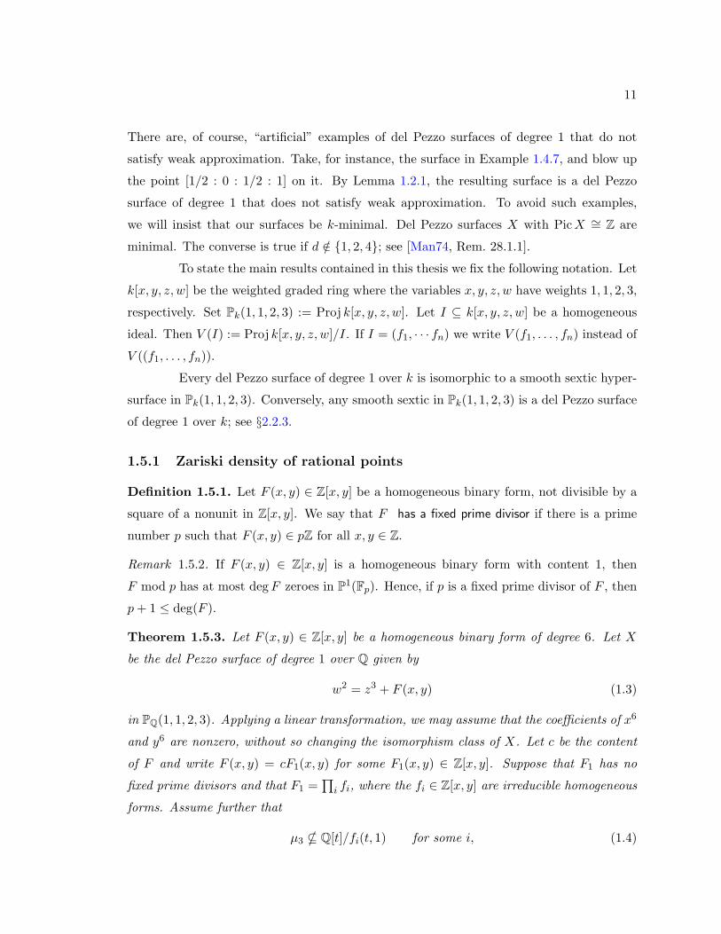
Theorem 1.5.3. Let F (x, y) ∈ Z[x, y] be a homogeneous binary form of degree 6. Let X

be the del Pezzo surface of degree 1 over Q given by

w2 = z3 + F (x, y) (1.3)

in PQ(1, 1, 2, 3). Applying a linear transformation, we may assume that the coefficients of x6

and y6 are nonzero, without so changing the isomorphism class of X. Let c be the content

of F and write F (x, y) = cF1(x, y) for some F1(x, y) ∈ Z[x, y]. Suppose that F1 has no

fixed prime divisors and that F1 =∏i fi, where the fi ∈ Z[x, y] are irreducible homogeneous

forms. Assume further that

µ3 * Q[t]/fi(t, 1) for some i, (1.4)

12

where µ3 is the group of third roots of unity. Finally, assume that Tate-Shafarevich groups

of elliptic curves over Q with j-invariant 0 are finite. Then the rational points of X are

dense for the Zariski topology.

Theorem 1.5.4. Let G[x, y] ∈ Z[x, y] be a homogeneous binary form of degree 4. Let X be

the del Pezzo surface of degree 1 over Q given by

w2 = z3 +G(x, y)z (1.5)

in PQ(1, 1, 2, 3). Applying a linear transformation, we may assume that the coefficients of

x4 and y4 are nonzero, without so changing the isomorphism class of X. Let c be the content

of G and write G(x, y) = cG1(x, y) for some G1(x, y) ∈ Z[x, y]. Suppose that G1 has no

fixed prime divisors and that G1 =∏i gi, where the gi ∈ Z[x, y] are irreducible homogeneous

forms. Assume further that

µ4 * Q[t]/gi(t, 1) for some i, (1.6)

where µ4 is the group of fourth roots of unity. Finally, assume that Tate-Shafarevich groups

of elliptic curves over Q with j-invariant 1728 are finite. Then the rational points of X are

dense for the Zariski topology.

The idea of the proof of Theorems 1.5.3 and 1.5.4 is as follows. Blowing-up the

canonical point of a del Pezzo surface of degree 1 gives an elliptic surface f : E → P1Q.

Assuming finiteness of Tate-Shafarevich groups, Nekovar, Dokchitser and Dokchitser have

shown that the root number of an elliptic curve E/Q is (−1)rank(E) (the parity conjecture;

see [Nek01, DD07]). It thus suffices to show that there are infinitely many fibers of f over

Q with negative root number (i.e., odd Mordell-Weil rank). In [Roh93], Rohrlich pioneered

the study of variations of root numbers on algebraic families of elliptic curves. We use his

formulas for local root numbers, together with those of Halberstadt and Rizzo [Hal98,Riz03]

to compute root numbers of elliptic curves associated to the del Pezzo surfaces of degree 1 of

Theorems 1.5.3 and 1.5.4. We then modify a sieve of Gouvea, Mazur, and Greaves [GM91,

Gre92] to search for infinitely many pairs of fibers with opposite root numbers. This gives

infinitely many fibers with odd rank, which proves the theorem.

The idea of studying density of rational points on an elliptic surface by looking

at variations in the root numbers of fibers is not new; the novelty in our approach lies in

the combination of sieving techniques from analytic number theory with explicit formulas

13

for root numbers. The reader is especially invited to look at [GM97] where the question of

potential density of rational points, i.e., Zariski density after a finite extension of the ground

field, is studied for elliptic surfaces with non-constant j-invariant. In contrast, the elliptic

surfaces we study in this thesis are all isotrivial.

We obtain the following corollary to Theorem 1.5.3, which addresses the question

of Zariski density of rational points for “diagonal” del Pezzo surface of degree 1 over Q.

Corollary 1.5.5. Let X be the del Pezzo surface of degree 1 over Q given as a sextic in

the weighted projective space PQ(1, 1, 2, 3) by

w2 = z3 +Ax6 +By6, (1.7)

where A and B are nonzero integers. Assume that Tate-Shafarevich groups of elliptic curves

over Q with j-invariant 0 are finite. If 3A/B is not a rational square, or if A and B are

relatively prime and 9 - AB, then the rational points of X are Zariski dense.

Remark 1.5.6. The restriction in (1.7) that A and B are integers is not severe. If A and B

are rational numbers, then one can clear denominators and rescale the variables to obtain

an equation of the the form (1.7). A similar comment applies for the restriction that

F (x, y) ∈ Z[x, y] in Theorem 1.5.3 and that G(x, y) ∈ Z[x, y] in Theorem 1.5.4.

Using our sieving technique, we will also show that the surfaces of Theorems 1.5.3

and 1.5.4 satisfy a variant of weak-weak approximation. We refer the reader to §3.5 for

details.

1.5.2 Weak approximation

We construct the following counterexamples to weak approximation.

Theorem 1.5.7. Let p ≥ 5 be a rational prime number such that p 6≡ 1 mod 12. Let X be

the del Pezzo surface of degree 1 over Q given by

w2 = z3 + p3x6 + p3y6

in PQ(1, 1, 2, 3). Then X is Q-minimal and there is a Brauer-Manin obstruction to weak ap-

proximation on X. Moreover, the obstruction arises from a cyclic algebra class in BrX/BrQ.

Remark 1.5.8. By Corollary 1.5.5, the above counterexamples to weak approximation have

a Zariski dense set of points, at least under the assumption that Tate-Shafarevich groups

of elliptic curves are finite.

14

To prove Theorem 1.5.7, we begin with an explicit study of the geometry of “di-

agonal” del Pezzo surfaces of degree 1 over an arbitrary field k with char k 6= 2, 3. These

are sextic surfaces of the form

w2 = z3 +Ax6 +By6 (1.8)

in the weighted projective space Pk(1, 1, 2, 3), where A,B ∈ k∗. The conditions A, B ∈ k∗

and char k 6= 2, 3, taken together, are equivalent to the smoothness of these surfaces. We

start by finding an explicit description of generators for the geometric Picard group for the

surfaces (1.8). More generally, we find explicit equations for all 240 exceptional curves on

any del Pezzo surface of degree 1 over any field.

Theorem 1.5.9. Let X be a del Pezzo surface of degree 1 over a field k, given as a smooth

sextic hypersurface V (f(x, y, z, w)) in Pk(1, 1, 2, 3). Let

Γ = V (z −Q(x, y), w − C(x, y)) ⊆ Pks(1, 1, 2, 3),

where Q(x, y) and C(x, y) are homogenous forms of degrees 2 and 3, respectively, in ks[x, y].

If Γ is a divisor on Xks, then it is an exceptional curve of X. Conversely, every exceptional

curve on X is a divisor of this form.

With explicit generators for PicXks , we may compute the cohomology group

H1(

Gal(ks/k),PicXks), which is a k-birational invariant of X; see [Man74, Theorem 23.3].

We derive the following theorem, analogous to [KT04, Thm. 1].

Theorem 1.5.10. Let k be a field with char k 6= 2, 3. Let X be a minimal del Pezzo surface

of degree 1 over k of the form (1.8). Then H1(

Gal(ks/k),Pic(Xks))

is isomorphic to one

of the following fourteen groups:

1; (Z/2Z)i, i ∈ 1, 2, 3, 4, 6, 8; (Z/3Z)j , j ∈ 1, 2, 3, 4;

(Z/6Z)k k ∈ 1, 2; Z/2Z× Z/6Z.

Each group occurs for some field k. When k = Q only the following seven groups occur:

1, Z/2Z, Z/2Z× Z/2Z, Z/2Z× Z/2Z× Z/2Z,

Z/3Z, Z/3Z× Z/3Z, Z/6Z.

15

Remark 1.5.11. In [Cor07, Theorem 4.1], Patrick Corn determines all the possible groups

that H1(

Gal ks/k,PicXks)

can be isomorphic to, for del Pezzo surfaces of degree 1. The

advantage of our work is that we can compute this cohomological invariant as a function of

A and B for surfaces of the form (1.8).

If, furthermore, k is a global field, then we may compute the group BrX/Br k, of

arithmetic interest, via the isomorphism

BrX/Br k ∼−→ H1(

Gal(ks/k),PicXks), (1.9)

obtained from the Hochschild-Serre spectral sequence; see §2.3.1 for the definition of BrX

and §2.3.4 for details on the Hochschild-Serre spectral sequence and the isomorphism (1.9).

To prove a statement like Theorem 1.5.7, we have to identify elements of BrX/Br k

explicitly. Given a cohomology class in H1(

Gal(ks/k),PicXks), it can be difficult to iden-

tify the corresponding element in BrX/Br k guaranteed by the isomorphism (1.9). We

present a simple strategy to search for cohomology classes in H1(

Gal(ks/k),PicXks)

which

correspond to cyclic algebras in the image of the natural map

BrX/Br k → Br k(X)/Br k,

where X is a locally soluble smooth geometrically integral variety over a global field k.

We hope that Theorem 4.4.3 will be of use to others wishing to calculate Brauer-Manin

obstructions to the Hasse principle and weak approximation via cyclic algebras on this wide

class of varieties.

16

Chapter 2

Background material

In this chapter we review some standard material from the theory of del Pezzo

surfaces and Brauer-Manin obstructions. We begin by outlining results of Coombes which

allow us to work with imperfect base fields.

The reader who is mainly interested in Chapter 3 is encouraged to skip §2.3; the

material in that section is relevant only for the results of Chapter 4.

2.1 Del Pezzo surfaces are separably split

Throughout this section, k denotes a separably closed field and k a fixed algebraic

closure of k. Recall that a collection of closed points in P2(k) is said to be in general position

if no 3 points lie on a line, no 6 points lie on a conic, and no 8 points lie on a singular cubic,

with one of the points at the singularity. Our goal is to prove the following strengthening

of [Man74, Theorem 24.4].

Theorem 2.1.1. Let X be a del Pezzo surface of degree d over k. Then either X is

isomorphic to the blow-up of P2k at 9 − d points in general position in P2(k), or d = 8 and

X is isomorphic to P1k × P1

k.

We need two results of Coombes, as follows.

Proposition 2.1.2 ([Coo88, Proposition 5]). Let f : X → Y be a birational morphism of

smooth projective surfaces over k. Then f factors as

X = X0 → X1 → · · · → Xr = Y,

17

where each map Xi → Xi+1 is a blow-up at a closed k-point of Xi+1.

The above proposition is well-known if we replace k with k. The main step in

the proof of Proposition 2.1.2 is to show that the blow-up at a closed point whose residue

field is a nontrivial purely inseparable extension of k cannot give rise to a smooth surface.

Using Iskovskikh’s classification theorem (Theorem 1.2.3), Coombes deduces the following

proposition.

Proposition 2.1.3 ([Coo88, Proposition 7]). The minimal smooth projective rational sur-

faces over k are P2k and the Hirzebruch surfaces Fn := P

(OP1

k⊕OP1

k(n)), where either n = 0

or n ≥ 2.

Finally, we need the following lemma.

Lemma 2.1.4 ([Man74, Theorem 24.3(ii)]). Let X be a del Pezzo surface over an alge-

braically closed field. Then every irreducible curve with negative self-intersection in excep-

tional.

Proof of Theorem 2.1.1. Let f : X → Y be a birational k-morphism with Y minimal, and

write

X = X0 → X1 → · · · → Xr = Y (2.1)

for a factorization of f as in Proposition 2.1.2. By Proposition 2.1.3 we need only consider

the following cases:

1. Y = P2k. We claim that no point that is blown-up in one step of the factorization (2.1)

may lie on the exceptional divisor of a previous blow-up: otherwise Xk would contain

a curve with self-intersection less than −1, contradicting Lemma 2.1.4. Hence X is

the blow-up of P2k at r distinct closed k-points. We conclude that d = K2

X = 9− r, as

claimed. Suppose that 3 of these points lie on a line L. Let f−1kLk denote the strict

transform of Lk for the base-extension fk : Xk → Yk. Then (f−1kLk, f

−1kLk) < −1, but

this is impossible by Lemma 2.1.4. Similarly, if 6 of the blown-up points lie on a conic

Q, or if 8 points lie on a singular cubic C with one of the points at the singularity, then

(f−1kQk, f

−1kQk) < −1, or (f−1

kCk, f

−1kCk) < −1, respectively, which is not possible.

Hence the blown-up points are in general position.

2. Y = P1k × P1

k. If X = Y then X is a del Pezzo surface of degree 8. Otherwise, we

may contract the two nonintersecting (−1)-curves of Xr−1 and obtain a birational

18

morphism φ : Xr−1 → P2k. We may use the map φ to construct a new birational

morphism X → P2k, given by

X = X0 → X1 → · · · → Xr−1φ−→ P2

k,

and thus we may reduce this case to the previous case.

3. Y = Fn, n ≥ 2. There is a curve C ⊆ (Fn)k whose divisor class satisfies (C,C) < −1.

Let f−1k

(C) denote the strict transform of C in Xk for the base-extension fk : Xk →(Fn)k. Then (f−1

kC, f−1

kC) < −1, but this is impossible by Lemma 2.1.4.

2.2 Further properties of del Pezzo surfaces

We review some well known facts about del Pezzo surfaces over a field k, be-

yond those stated in §1.3 and in the previous section. The basic references on the subject

are [Man74], [Dem80] and [Kol96, III.3].

2.2.1 The Picard group

Let X be a del Pezzo surface over a field k of degree d. Recall that an exceptional

curve on X is an irreducible curve C on Xk such that (C,C) = (C,KX) = −1. Theo-

rem 2.1.1 shows that exceptional curves on X are already defined over ks. The number of

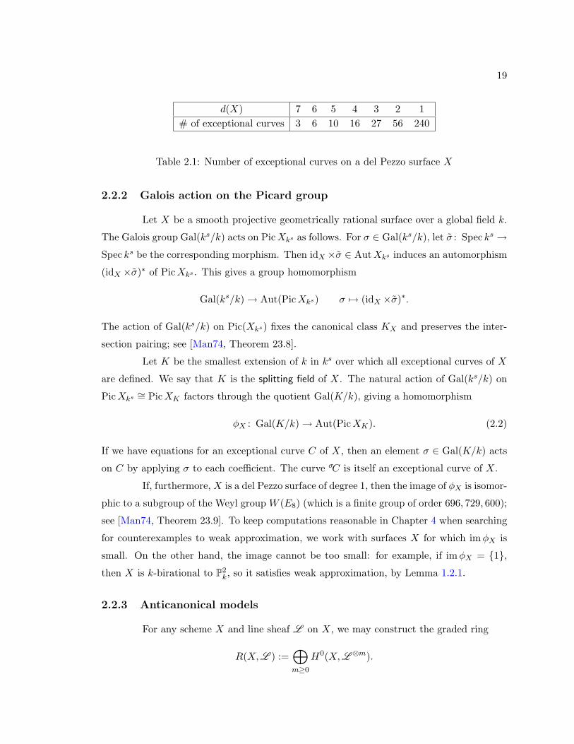
exceptional curves on X varies with d as shown in Table 2.1.

We have seen that if Xks P1ks × P1

ks then Xks is isomorphic to a blow-up of P2ks

at r := 9−d closed points P1 . . . , Pr in general position. It follows that the group PicXks

is isomorphic to Z10−d (see [Har77, Proposition V.3.2]); if d ≤ 7 then it is generated by the

classes of exceptional curves. Let ei be the class of an exceptional curve corresponding to

Pi under the blow-up map, and let ` be the class of the pullback of a line in P2ks not passing

through any of the Pi. Then e1, . . . , er, ` is a basis for PicXks . Note that

(ei, ej) = −δij , (ei, `) = 0, (`, `) = 1,

where δij is the usual Kronecker delta function. With respect to this basis, the anticanonical

class is given by −KX = 3`−∑ei.

19

d(X) 7 6 5 4 3 2 1# of exceptional curves 3 6 10 16 27 56 240

Table 2.1: Number of exceptional curves on a del Pezzo surface X

2.2.2 Galois action on the Picard group

Let X be a smooth projective geometrically rational surface over a global field k.

The Galois group Gal(ks/k) acts on PicXks as follows. For σ ∈ Gal(ks/k), let σ : Spec ks →Spec ks be the corresponding morphism. Then idX ×σ ∈ AutXks induces an automorphism

(idX ×σ)∗ of PicXks . This gives a group homomorphism

Gal(ks/k)→ Aut(PicXks) σ 7→ (idX ×σ)∗.

The action of Gal(ks/k) on Pic(Xks) fixes the canonical class KX and preserves the inter-

section pairing; see [Man74, Theorem 23.8].

Let K be the smallest extension of k in ks over which all exceptional curves of X

are defined. We say that K is the splitting field of X. The natural action of Gal(ks/k) on

PicXks∼= PicXK factors through the quotient Gal(K/k), giving a homomorphism

φX : Gal(K/k)→ Aut(PicXK). (2.2)

If we have equations for an exceptional curve C of X, then an element σ ∈ Gal(K/k) acts

on C by applying σ to each coefficient. The curve σC is itself an exceptional curve of X.

If, furthermore, X is a del Pezzo surface of degree 1, then the image of φX is isomor-

phic to a subgroup of the Weyl group W (E8) (which is a finite group of order 696, 729, 600);

see [Man74, Theorem 23.9]. To keep computations reasonable in Chapter 4 when searching

for counterexamples to weak approximation, we work with surfaces X for which imφX is

small. On the other hand, the image cannot be too small: for example, if imφX = 1,then X is k-birational to P2

k, so it satisfies weak approximation, by Lemma 1.2.1.

2.2.3 Anticanonical models

For any scheme X and line sheaf L on X, we may construct the graded ring

R(X,L ) :=⊕m≥0

H0(X,L ⊗m).

20

When L = ω⊗−1X , we call R(X,ω⊗−1

X ) the anticanonical ring of X. If X is a del Pezzo

surface then X is isomorphic to the scheme ProjR(X,ω⊗−1X ) [Kol96, Theorem III.3.5]. This

scheme is known as the anticanonical model of the del Pezzo surface.

The construction of anticanonical models is reminiscent of the procedure that

yields a Weierstrass model of an elliptic curve. In fact, we can use the Riemann-Roch

theorem for surfaces to prove the following dimension formula for a del Pezzo surface X

over k of degree d:

h0(X,−mKX

)=m(m+ 1)

2d+ 1; (2.3)

see [Kol96, Corollary III.3.2.5] or [CO99]. If X has degree 1, then the anticanonical model

for X is a smooth sextic hypersurface in Pk(1, 1, 2, 3), and we may compute such a model,

up to isomorphism, as follows:

1. Choose a basis x, y for the 2-dimensional k-vector space H0(X,−KX

).

2. The elements x2, xy, y2 of H0(X,−2KX

)are linearly independent. However,

h0(X,−2KX

)= 4; choose an element z to get a basis x2, xy, y2, z for this k-vector

space.

3. The elements x3, x2y, xy2, y3, xz, yz of H0(X,−3KX

)are linearly independent, but

h0(X,−3KX

)= 7. Choose an element w to get a basis x3, x2y, xy2, y3, xz, yz, w for

this k-vector space.

4. The vector space H0(X,−6KX

)is 22-dimensional, so the 23 elements

x6, x5y, x4y2, x3y3, x2y4, xy5, y6, x4z, x3yz, x2y2z, xy3z,

y4z, x2z2, xyz2, y2z2, z3, x3w, x2yw, xy2w, y3w, xzw, yzw,w2

must be k-linearly dependent. Let f(x, y, z, w) = 0 be a linear dependence relation

among these elements. Then an anticanonical model of X is Proj k[x, y, z, w]/(f),

where x, y, z, w are variables with weights 1, 1, 2 and 3 respectively. This way X may

be described as the (smooth) sextic hypersurface V (f) in Pk(1, 1, 2, 3).

For more details on this construction, see [CO99, pp.1199–1201].

Remark 2.2.1. If k is a field of characteristic not equal to 2 or 3, then in step (4) above we

may complete the square with respect to the variable w and the cube with respect to the

21

variable z to obtain an equation f(x, y, z, w) = 0 involving only the monomials

x6, x5y, x4y2, x3y3, x2y4, xy5, y6, x4z, x3yz, x2y2z, xy3z, y4z, z3, w2.

Moreover, we may also rescale the variables so that the coefficients of w2 and z3 are ±1.

Remark 2.2.2. If X has degree d ≥ 3, then the anticanonical model recovers the usual

description of X as a smooth degree d surface in Pdk. In particular, when d = 3 we get a

smooth cubic surface in P3k. If X has degree 2 then the anticanonical model is a quartic

hypersurface in the weighted projective space Pk(1, 1, 1, 2); such a surface can then be

thought of as a double cover of a P2k ramified along a quartic curve.

Remark 2.2.3. If we write a del Pezzo surface X of degree 1 over a field k as the smooth

sextic hypersurface V (f(x, y, z, w)) in Pk(1, 1, 2, 3), then x, y is a basis for H0(X,−KX

)and x2, xy, y2, z is a basis for H0

(X,−2KX

). In particular, the base point of |−KX | is

[0 : 0 : 1 : 1].

2.2.4 Del Pezzo surfaces of degree 1 and elliptic surfaces

Let X be a del Pezzo surface of degree 1 over a field k. Recall that the anticanonical

linear system |−KX | contains a single (k-rational) base-point (see §1.4); we call this point

the anticanonical point of X. By (2.3) we have h0(X,−KX) = 2, and thus the linear system

|−KX | gives rise to a rational map f : X 99K P1k; this map is regular everywhere except

at the anticanonical point O. Blowing-up O to resolve the indeterminacy of f we obtain a

commutative diagram

E

~~~~

~~~~

ρ

Xf //___ P1

k

Almost all of the fibers of ρ are nonsingular genus 1 curves. The morphism ρ restricts to

an isomorphism between the exceptional divisor of E and P1k. This gives a distinguished

section O : P1k → E of ρ, making (ρ,O) into an elliptic surface.

Concretely, if X is given by a smooth sextic

w2 = z3 + F (x, y)z2 +G(x, y)z +H(x, y)

in Pk(1, 1, 2, 3), then O = [0 : 0 : 1 : 1]; see Remark 2.2.3. In this case, E is the subscheme

of Pk(1, 1, 2, 3)× P1k = Proj(k[x, y, z, w])× Proj(k[m,n]) cut out by the equations

w2 = z3 + F (x, y)z2 +G(x, y)z +H(x, y) and nx−my = 0. (2.4)

22

The map ρ : E → P1k is then given by ([x : y : z : w], [m : n]) 7→ [m : n]. Note that for points

away from the exceptional divisor we have [m : n] = [x : y].

Let t be the rational function m/n, so that x = ty on E . The generic fiber E/k(t)

of ρ is the curve

E : w2 = z3 + y2F (t, 1)z2 + y4G(t, 1)z + y6H(t, 1) (2.5)

in Proj(k(t)[y, z, w]). On the affine chart Spec(k(t)[z/y2, w/y3]) of this weighted ambient

space, the curve (2.5) is isomorphic to the affine curve

(w/y3)2 = (z/y2)3 + F (t, 1)(z/y2)2 +G(t, 1)(z/y2) +H(t, 1).

Relabelling the variables, we find that the elliptic curve E/k(t) is given by the Weierstrass

model

y2 = x3 + F (t, 1)x2 +G(t, 1)x+H(t, 1).

Similarly, we can also check that the fiber of ρ above [m : n] ∈ P2k(k) is isomorphic to the

curve in P2k with affine equation given by

y2 = x3 + F (m,n)x2 +G(m,n)x+H(m,n).

2.3 Brauer-Manin obstructions

Let X be a nice variety over a global field k. We have seen that the inclusion

X(k) ⊆ X(Ak) gives a necessary condition for the existence of a k-rational point on X,

namely, X(Ak) 6= ∅. This condition is relatively easy to check in practice. For example, the

Lang-Weil bounds, together with Hensel’s lemma ensure the existence of kv-points for all but

finitely many v ∈ Ωk. We have also seen that the condition X(Ak) 6= ∅ need not guarantee

the existence of a k-rational point on X. To explain some counterexamples to the Hasse

principle, in [Man71] Manin introduced an obstruction based on a set X(Ak)Br ⊆ X(Ak)

containing the closure for the adelic topology of X(k) in X(Ak):

X(k) ⊆ X(Ak)Br ⊆ X(Ak). (2.6)

Definition 2.3.1. Let X be a nice variety over a global field k. We say there is a

• Brauer-Manin obstruction to the Hasse principle if X(Ak) 6= ∅ but X(Ak)Br = ∅;

• Brauer-Manin obstruction to weak approximation if X(Ak) \X(Ak)Br 6= ∅.

23

2.3.1 The Brauer group of a scheme

The set X(Ak)Br is defined using the Brauer group of X, which is in turn defined

using either Azumaya algebras or etale cohomology, as follows.

Definition 2.3.2. An Azumaya algebra on a scheme X is an OX -algebra A that is coherent

and locally free as an OX -module, such that the fiber A(x) := A ⊗OX,x k(x) is a central

simple algebra over the residue field k(x) for each x ∈ X.

Two Azumaya algebras A and B on X are similar if there exist locally free coherent

OX -modules E and F such that

A⊗OX EndOX (E) ∼= B ⊗OX EndOX (F).

Definition 2.3.3. The Azumaya Brauer group of a scheme X is the set of similarity classes

of Azumaya algebras on X, with multiplication induced by tensor product of sheaves. We

denote this group by BrAzX.

The inverse of [A] ∈ BrAzX is the class [Aop] of the opposite algebra of A; the

identity element is [OX ] (see [Gro68a, p. 47]).

Definition 2.3.4. The Brauer group of a scheme X is BrX := H2et

(X,Gm

).

Remark 2.3.5. If F is a field, then Br SpecF = BrF , the usual Brauer group of a field. The

Brauer group is a contravariant functor on schemes, with values in the category of abelian

groups.

For any scheme X there is a natural inclusion

BrAzX → BrX;

see [Mil80, Theorem IV.2.5]. The following result of Gabber, a proof of which can be found

in [dJ], determines the image of this injection for a scheme with some kind of polarization.

Theorem 2.3.6 (Gabber, de Jong). If X is a scheme endowed with an ample invertible

sheaf then the natural map BrAzX → BrX induces an isomorphism

BrAzX∼−→ (BrX)tors.

24

If X is an integral scheme with function field k(X), then the inclusion Spec k(X)→X gives rise to a map BrX → Br k(X) via functoriality of etale cohomology. If further X is

regular and quasi-compact then this induced map is injective; see [Mil80, Example III.2.22].

On the other hand, the group Br k(X) is torsion, because it is a Galois cohomology group.

These two facts imply the following corollary of Theorem 2.3.6.

Corollary 2.3.7. Let X be a regular quasiprojective variety over a field. Then

BrAzX ∼= BrX.

Finally, we note that the Brauer group of well-behaved low dimensional schemes

over a field is a birational invariant.

Theorem 2.3.8 ([Gro68b, Corollaire III.7.5]). Let X be a nice k-variety of dimension at

most 2. Then BrX depends only on the birational class of X.

Corollary 2.3.9. Let X be a nice geometrically rational surface over a field k. Then

BrXks = 0.

Proof. This follows directly from Theorem 2.3.8 and the fact that BrP2ks = 0; see [Mil70, p.

305].

2.3.2 The Brauer-Manin set

Let X be a nice variety over a global field k. For each A ∈ BrX and each field

extension K/k there is a specialization map

evA : X(K)→ BrK, x 7→ Ax ⊗OX,x K.

These specialization maps may be put together to construct a pairing

φ : BrX ×X(Ak)→ Q/Z, (A, (xv)) 7→∑v∈Ωk

invv(evA(xv)), (2.7)

where invv : Br kv → Q/Z is the usual invariant map from local class field theory. The sum

in (2.7) is in fact finite because for (xv) ∈ X(Ak) we have evA(xv) = 0 ∈ Br kv for all but

finitely many v; see [Sko01, p. 101]. For A ∈ BrX we obtain a commutative diagram

X(k) //

evA

X(Ak)

evA

φ(A,−)

((QQQQQQQQQQQQQQ

0 // Br k //⊕

v Br kvPv invv // Q/Z // 0

(2.8)

25

where the bottom row is the usual exact sequence from class field theory.

We are now ready to define the intermediate set in (2.6).

Definition 2.3.10. Let X be a nice variety over a global field k, and let A ∈ BrX. Let

X(Ak)A :=

(xv) ∈ X(Ak) : φ(A, (xv)) = 0.

We call

X(Ak)Br :=⋂

A∈BrX

X(A)A

the Brauer-Manin set of X.

Remark 2.3.11. The commutativity of the diagram (2.8), together with the fact that the

bottom row is a complex, implies that X(k) ⊆ X(Ak)Br. Moreover, if Q/Z is given the

discrete topology, then the map φ(A,−) : X(Ak) → Q/Z is continuous, so X(Ak)A is a

closed subset of X(Ak); see [Har04, §3.1]. This shows that X(k) ⊆ X(Ak)Br.

Remark 2.3.12. The structure map X → Spec k gives rise to a map Br k → BrX which is

injective if X(Ak) 6= ∅; see §2.3.4 below. The exactness of the bottom row of (2.8) then

implies that to compute⋂A∈BrX X(Ak)A it is enough to calculate the intersection over a

set of representatives for the group BrX/Br k.

2.3.3 Conjectures of Colliot-Thelene and Sansuc

Hasse principle and weak approximation. All the counterexamples to the Hasse princi-

ple and weak approximation in Chapter 1 can be explained by a Brauer-Manin obstruction.

In [CTS80, question k1], Colliot-Thelene and Sansuc ask whether for a smooth projective

geometrically rational surface X over a global field k, the Brauer-Manin obstruction to the

Hasse principle is the “only one,” i.e.,

does the implication X(Ak)Br 6= ∅ =⇒ X(k) 6= ∅ hold? (2.9)

One may ask a similar question for weak approximation:

does the equality X(k) = X(Ak)Br hold? (2.10)

Colliot-Thelene and Sansuc had affirmative answers to these questions in mind, based on

evidence eventually published in the papers [CTCS80, CTS82]. In the case of weak ap-

proximation, equality (2.10) is known to be true for del Pezzo surfaces of degree at least 4

26

(the case of degree 4 is a hard theorem of Salberger and Skorobogatov [SS91]). Numerical

evidence for the case of the Hasse principle on surfaces of degrees 3 and 2 has been gathered

in [CTKS87,Cor05].

In [CT03], these questions about the uniqueness of the Brauer-Manin obstruction

are generalized and the following far-reaching conjecture is proposed.

Conjecture 2.3.13 (Colliot-Thelene). Let X be a smooth proper geometrically integral

variety over a global field k. Suppose that X is geometrically rationally connected. Then

the Brauer-Manin obstruction to the Hasse principle and weak approximation for X is the

only one.

Not all counterexamples to the Hasse-principle and weak approximation can be

explained by a Brauer-Manin obstruction. Skorobogatov gave the first unconditional ex-

amples of the insufficiency of this obstruction: he produced a bi-elliptic surface that has

no rational points and which nonetheless has a nonempty Brauer-Manin set; see [Sko99].

Harari and Skorobogatov have constructed examples of Enriques surfaces that fail to satisfy

weak approximation, but for which the containment X(k) ⊆ X(Ak)Br is strict; see [Har00,

HS05]. Recently, Poonen constructed certain Chatelet surface bundles whose lack of rational

points cannot be explained directly by any known cohomologically constructed obstruction;

see [Poo08].

Weak-weak approximation. Unirational varieties are expected to satisfy weak-weak

approximation.

Conjecture 2.3.14 (Colliot-Thelene [Ser08, p. 30]). Let X be a smooth proper geometri-

cally integral variety over a number field k. If X is unirational then it satisfies weak-weak

approximation.

Colliot-Thelene and Ekedahl have shown that if Conjecture 2.3.14 holds then the

inverse Galois problem could be solved over Q, i.e., every finite group is a Galois group over

Q; see [Ser08, Theorem 3.5.9].

2.3.4 The Hochschild-Serre spectral sequence in etale cohomology

Let X be a nice locally soluble variety over a global field k. By Remark 2.3.12, to

compute X(Ak)Br it suffices to compute the intersection of X(A)A over a set of representa-

27

tives for the group BrX/Br k. If BrXks = 0, then the Hochschild-Serre spectral sequence

in etale cohomology provides a tool for computing the group BrX/Br k.

Let K be a finite Galois extension of k, with Galois group G. The Hochschild-Serre

spectral sequence

Ep,q2 := Hp(G,Hq

et

(XK ,Gm

))=⇒ Hp+q

et

(X,Gm

)=: Lp+q

gives rise to the usual “low-degree” long exact sequence

0→ E1,02 → L1 → E0,1

2 → E2,02 → ker

(L2 → E0,2

2

)→ E1,1

2 → E3,02

which in our case is

0→ PicX → (PicXK)G → H2(G,K∗

)→ ker(BrX → BrXK)

→ H1(G,PicXK

)→ H3

(G,K∗

).

(2.11)

Taking the direct limit over all finite Galois extensions of k gives the exact sequence

0→ PicX → (PicXks)Gal(ks/k) → Br k → ker(BrX → BrXks)

→ H1(

Gal(ks/k),PicXks)→ H3

(Gal(ks/k), ks∗

).

(2.12)

Furthermore, if k is a global field, then H3(

Gal(ks/k), ks∗)

= 0; this fact is due to Tate—

see [NSW08, 8.3.11(iv), 8.3.17].

For each v ∈ Ωk, local solubility of X gives a morphism Spec kv → X that splits

the base extension πv : Xkv → Spec kv of the structure map of X. Thus, by functoriality

of the Brauer group, the natural maps π∗v : Br kv → BrXkv split for every v ∈ Ωk. The

exactness of the bottom row of (2.8) then shows that the natural map Br k → BrX coming

from the structure morphism of X is injective. Moreover, if X is a del Pezzo surface, then

BrXks = 0 by Corollary 2.3.9 and thus (2.12) gives rise the to short exact sequence

0→ Br k → BrX → H1(

Gal(ks/k),PicXks)→ 0.

If K is a splitting field for X then the inflation map

H1(

Gal(K/k),PicXK

)→ H1

(Gal(ks/k),PicXks

)is an isomorphism, because the cokernel maps into the first cohomology group of a free

Z-module with trivial action by a profinite group, which is trivial. Hence

BrX/Br k ∼= H1(

Gal(K/k),PicXK

). (2.13)

28

Finally, we note that since X(Ak) 6= ∅, if H is a subgroup of G, then by (2.11) and

the injectivity of the map Br k → BrX, we know that

PicXKH∼−→ (PicXK)H , (2.14)

where KH is the fixed field of K by H. It will be important for us in Chapter 4 to make

this isomorphism explicit. This is the subject of the next section.

2.3.5 Galois descent of line bundles

To make the isomorphism (2.14) explicit we need the theory of Galois descent

of line sheaves, which is a special case of the theory of descent of quasi-coherent sheaves

over faithfully flat and quasi-compact morphisms. Good references for Galois descent are

[BLR90] and [KT06]. For the general theory of descent see [Gro03].

Let K/k be a finite Galois extension of global fields. For every element σ ∈Gal(K/k) let σ : SpecK → SpecK denote the corresponding morphism. Let X be a k-

scheme, and suppose we are given a line bundle F on the K-scheme XK , together with a

collection of isomorphisms1 fσ : F → σ∗F such that

fτσ = σfτ fσ for all σ, τ ∈ Gal(K/k), (2.15)

where σfτ := σ∗fτ . Then there exists a sheaf F on X, and an isomorphism λ : FK → F

such that fσ = σλ λ−1 for all σ. Together, the equalities (2.15) are referred to as the

cocycle condition.

If X is a geometrically integral k-scheme, then F = OXK (D) for some divisor

D ∈ DivXK , and fσ can be regarded as a function (up to multiplication by a scalar) whose

associated divisor is D−σD. If X(k) 6= ∅ then one may use a point in P ∈ X(k) to normalize

the functions so that fσ acts as the identity in the fiber of F at P . We usually do not know

if X(k) is empty or not, but in the case of del Pezzo surfaces of degree 1 over k we have the

anticanonical point.

To obtain a divisor for the descended line bundle, we take a rational section ξ of

F and we “average it” over the Galois group G to obtain a rational section of F

s :=∑σ∈G

σ−1(fσ(ξ)).

1Here we use a slight abuse of notation: we write σ∗ for the automorphism of XK induced by theautomorphism σ∗ of SpecK.

29

Note that it may be necessary to change the choice of ξ to make s nonzero. The divisor

of zeroes of s, with respect to local trivializations for F , gives a line bundle isomorphic to

the descended line bundle. We often use the rational section ξ = 1, and since fσ acts by

multiplication, we obtain s =∑

σ∈Gσ−1

(fσ) in this case.

30

Chapter 3

Zariski density of rational points

on del Pezzo surfaces of degree 1

In this chapter we study the question of Zariski density of Q-rational points for

del Pezzo surfaces of degree 1 of the form

w2 = z3 + F (x, y) or w2 = z3 +G(x, y)z

in PQ(1, 1, 2, 3), where F and G are homogeneous integral forms of degree 6 and 4, respec-

tively. Our goal is to prove Theorems 1.5.3 and 1.5.4, as well as Corollary 1.5.5. Blowing

up the anticanonical point [0 : 0 : 1 : 1] on these surfaces gives elliptic surfaces E → P1Q,

where the fiber above the point [m : n] ∈ P1Q(Q) is isomorphic to the plane cubic curve

y2 = x3 + F (m,n) or y2 = x3 +G(m,n)x, (3.1)

respectively; see §2.2.4. This cubic curve is an elliptic curve for all but finitely many [m : n].

We investigate the parity of the Mordell-Weil rank of these elliptic curves in an effort to

produce many rational points on the original del Pezzo surfaces. Our main tools are a

detailed study of the root numbers of the elliptic curves

y2 = x3 + α and y2 = x3 + αx (α 6= 0), (3.2)

and a “pseudo squarefree” sieve that allows us to produce infinite families of elliptic curves

of the form (3.1) with opposite Mordell-Weil parity ; see Remarks 3.1.7 and 3.1.11.

Following a suggestion of Colliot-Thelene, we prove in §3.5 that the surfaces of

Theorems 1.5.3 and 1.5.4 satisfy a variant of weak-weak approximation.

31

Throughout, for a prime p ∈ Z we denote the corresponding p-adic valuation by

vp. If a is a nonzero integer then(a

p

)will denote the usual Legendre symbol; if m is an

odd positive integer then(a

m

)will denote the usual Jacobi symbol.

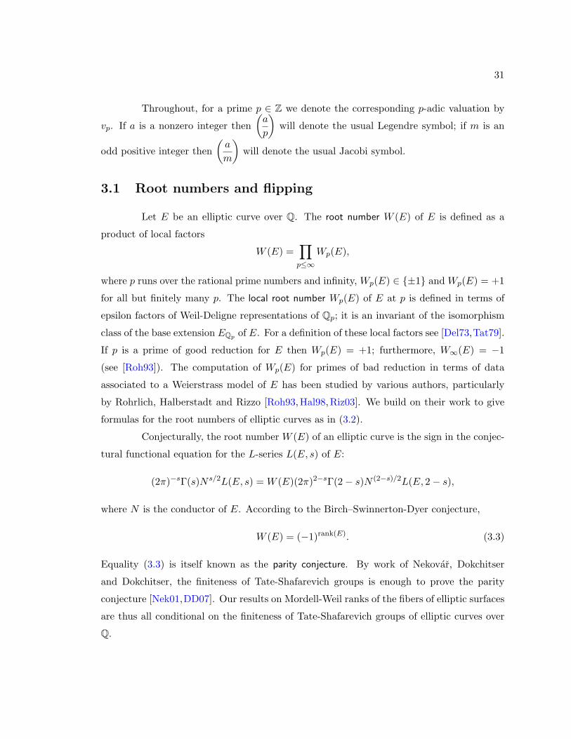
3.1 Root numbers and flipping

Let E be an elliptic curve over Q. The root number W (E) of E is defined as a

product of local factors

W (E) =∏p≤∞

Wp(E),

where p runs over the rational prime numbers and infinity, Wp(E) ∈ ±1 and Wp(E) = +1

for all but finitely many p. The local root number Wp(E) of E at p is defined in terms of

epsilon factors of Weil-Deligne representations of Qp; it is an invariant of the isomorphism

class of the base extension EQp of E. For a definition of these local factors see [Del73,Tat79].

If p is a prime of good reduction for E then Wp(E) = +1; furthermore, W∞(E) = −1

(see [Roh93]). The computation of Wp(E) for primes of bad reduction in terms of data

associated to a Weierstrass model of E has been studied by various authors, particularly

by Rohrlich, Halberstadt and Rizzo [Roh93, Hal98, Riz03]. We build on their work to give

formulas for the root numbers of elliptic curves as in (3.2).

Conjecturally, the root number W (E) of an elliptic curve is the sign in the conjec-

tural functional equation for the L-series L(E, s) of E:

(2π)−sΓ(s)N s/2L(E, s) = W (E)(2π)2−sΓ(2− s)N (2−s)/2L(E, 2− s),

where N is the conductor of E. According to the Birch–Swinnerton-Dyer conjecture,

W (E) = (−1)rank(E). (3.3)

Equality (3.3) is itself known as the parity conjecture. By work of Nekovar, Dokchitser

and Dokchitser, the finiteness of Tate-Shafarevich groups is enough to prove the parity

conjecture [Nek01,DD07]. Our results on Mordell-Weil ranks of the fibers of elliptic surfaces

are thus all conditional on the finiteness of Tate-Shafarevich groups of elliptic curves over

Q.

32

3.1.1 The root number of Eα/Q : y2 = x3 + α

Let α be a nonzero integer. We give a closed formula for the root number of the

elliptic curve Eα/Q : y2 = x3 + α, in terms of α. Throughout, we write W (α) for this root

number and Wp(α) for the local root number of Eα at p. We begin by determining W2(α)

and W3(α).

Lemma 3.1.1. Let α be a nonzero integer. Define α2 and α3 by α = 2v2(α)α2 = 3v3(α)α3.

Then

W2(α) =

−1 if v2(α) ≡ 0 or 2 mod 6;

or if v2(α) ≡ 1, 3, 4 or 5 mod 6 and α2 ≡ 3 mod 4;

+1 otherwise,

W3(α) =

−1 if v3(α) ≡ 1 or 2 mod 6 and α3 ≡ 1 mod 3;

or if v3(α) ≡ 4 or 5 mod 6 and α3 ≡ 2 mod 3;

or if v3(α) ≡ 0 mod 6 and α3 ≡ 5 or 7 mod 9;

or if v3(α) ≡ 3 mod 6 and α3 ≡ 2 or 4 mod 9,

+1 otherwise.

Proof. According to [Riz03, §1.1], to determine the local root number at p of an elliptic

curve given in Weierstrass form, we must find the smallest vector with nonnegative entries

(a, b, c) := (vp(c4), vp(c6), vp(∆)) + k(4, 6, 12) (3.4)

for k ∈ Z, where c4, c6 and ∆ are the usual quantities associated to a Weierstrass equation

(see [Sil92, Ch. III]). For the curves in question we have

c4 = 0, c6 = −25 · 33 · α, and ∆ = −24 · 33 · α2,

whence

(vp(c4), vp(c6), vp(∆)) = (∞, vp(α), 2vp(α)) +

(0, 5, 4) if p = 2,

(0, 3, 3) if p = 3,

Now it is a simple matter of using the tables in [Riz03, §1.1] to compute local root numbers.

We illustrate the computation of W2(α) in one example. Suppose that v2(α) ≡ 4 mod

6. Then (a, b, c) = (∞, 3, 0), and according to the entries under (≥ 4, 3, 0) in Table III

33

of [Riz03], we have W2(α) = −1 if and only if c′6 := c6/2v2(c6) ≡ 3 mod 4, i.e., if and only

if α2 ≡ 3 mod 4. All other local root number computations are similar and we omit the

details.

Remark 3.1.2. We take the opportunity to note that the entry (≥5, 6, 9) in Table II of [Riz03]

has a typo. The “special condition” should read c′6 6≡ ±4 mod 9.

Remark 3.1.3. In [Liv95], Liverance gives a closed formula for the global root number of

curves of the form y2 = x3 + α, where α is a sixth-power free integer. However, what he

calls w2 and w3 in his formula are not the local root numbers at 2 and 3, respectively, for

these curves.

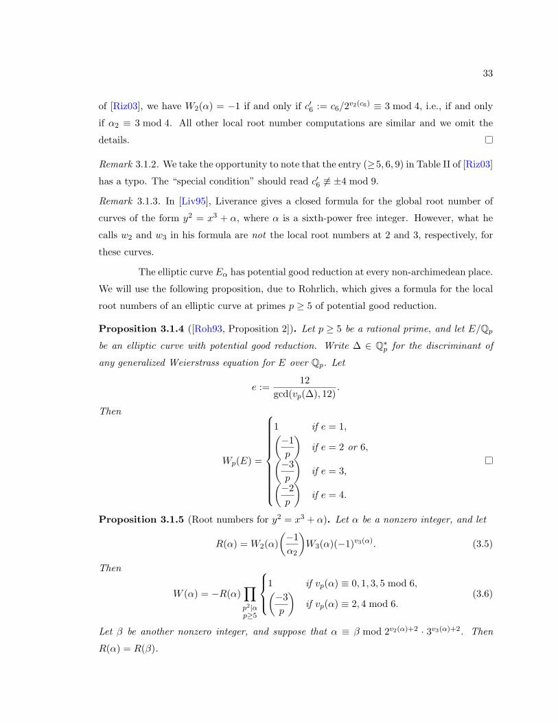
The elliptic curve Eα has potential good reduction at every non-archimedean place.

We will use the following proposition, due to Rohrlich, which gives a formula for the local

root numbers of an elliptic curve at primes p ≥ 5 of potential good reduction.

Proposition 3.1.4 ([Roh93, Proposition 2]). Let p ≥ 5 be a rational prime, and let E/Qpbe an elliptic curve with potential good reduction. Write ∆ ∈ Q∗p for the discriminant of

any generalized Weierstrass equation for E over Qp. Let

e :=12

gcd(vp(∆), 12).

Then

Wp(E) =

1 if e = 1,(−1p

)if e = 2 or 6,(

−3p

)if e = 3,(

−2p

)if e = 4.

Proposition 3.1.5 (Root numbers for y2 = x3 + α). Let α be a nonzero integer, and let

R(α) = W2(α)(−1α2

)W3(α)(−1)v3(α). (3.5)

Then

W (α) = −R(α)∏p2|αp≥5

1 if vp(α) ≡ 0, 1, 3, 5 mod 6,(−3p

)if vp(α) ≡ 2, 4 mod 6.

(3.6)

Let β be another nonzero integer, and suppose that α ≡ β mod 2v2(α)+2 · 3v3(α)+2. Then

R(α) = R(β).

34

Proof. Since ∆(Eα) = −2433α2, applying Proposition 3.1.4 we obtain

W (α) = −W2(α)W3(α)∏p |αp≥5

1 if vp(α) ≡ 0 mod 6,(−1p

)if vp(α) ≡ 1, 3, 5 mod 6,(

−3p

)if vp(α) ≡ 2, 4 mod 6.

(3.7)

Let r be the product of the primes p ≥ 5 such that vp(α) = 1, let b = α/r and set

α2 :=α

2v2(α), b2 :=

b

2v2(b).

Note that r = α2/b2 = α/b. We may rewrite (3.7) as

W (α) = −W2(α)W3(α)(−1r

)∏p | bp≥5

1 if vp(α) ≡ 0 mod 6,(−1p

)if vp(α) ≡ 1, 3, 5 mod 6,(

−3p

)if vp(α) ≡ 2, 4 mod 6.

(3.8)

On the other hand, we have(−1r

)=(−1α2/b2

)=(−1α2

)·(−1b2

)=(−1α2

)·(−13

)v3(α)

·∏p | bp≥5

(−1p

)vp(α)

,

so we can write (3.8) as

W (α) = −[W2(α)

(−1α2

)W3(α)(−1)v3(α)

]∏p | bp≥5

(−1p

)vp(α)

if vp(α) ≡ 0 mod 6,(−1p

)1+vp(α)

if vp(α) ≡ 1, 3, 5 mod 6,(−3p

)·(−1p

)vp(α)

if vp(α) ≡ 2, 4 mod 6,

= −R(α)∏p2 |αp≥5

1 if vp(α) ≡ 0, 1, 3, 5 mod 6,(−3p

)if vp(α) ≡ 2, 4 mod 6.

as desired, because p | b, p ≥ 5 ⇐⇒ p2 |α, p ≥ 5.

To prove the last claim of the theorem, note that if α ≡ β mod 2v2(α)+2 · 3v3(α)+2

then v2(α) = v2(β), v3(α) = v3(β) and we have

α

2v2(α)≡ β

2v2(β)mod 4 and

α

3v3(α)≡ β

3v3(β)mod 9.

The claim now follows from Lemma 3.1.1

35

The following corollary describes conditions on two nonzero integers α and β which

guarantee that the elliptic curves y2 = x3 +α and y2 = x3 + β have opposite root numbers.

This is one of the key inputs to the proof of Theorem 1.5.3.

Corollary 3.1.6 (Flipping I). Let α, β be nonzero integers such that

1. α ≡ β mod 2v2(α)+2 · 3v3(α)+2,

2. α = c`, where ` is squarefree and gcd(c, `) = 1,

3. β = cq2+6kη, where η is square free, gcd(c, η) = gcd(q, cη) = 1, k ≥ 0, q ≥ 5 is prime

and q ≡ 2 mod 3.

Then W (α) = −W (β).

Proof. The first condition ensures that R(α) = R(β). Since ` is squarefree and gcd(c, `) = 1,

the only primes greater than 3 contributing to W (α) are those whose square divides c.

Similarly, since η is squarefree and gcd(c, η) = gcd(q, η) = 1, the only primes greater than

3 contributing to W (β) are those whose square divides c, and q. Since gcd(q, c) = 1, q ≥ 5

and q ≡ 2 mod 3, we have

W (β) =(−3q

)W (α) = −W (α)

Remark 3.1.7. To prove Zariski density of rational points on the elliptic surface E → P1Q

associated to a del Pezzo of degree 1 as in Theorem 1.5.3, it is enough to do the following.

First, prove that there exist infinite sets F1 and F2 of coprime pairs of integers such that

whenever (m1, n1) ∈ F1 and (m2, n2) ∈ F2 then

1. α := F (m1, n1) and β := F (m2, n2) are nonzero integers.

2. α ≡ β mod 2v2(α)+2 · 3v3(α)+2,



and q ≡ 2 mod 3.

Then, by Corollary 3.1.6, we know that either

W (F (m,n)) = −1 for all (m,n) ∈ F1,

36

or

W (F (m,n)) = −1 for all (m,n) ∈ F2.

Hence, there are infinitely many closed fibers of E → P1Q with negative root number. As-

suming the parity conjecture, this gives an infinite number of closed fibers with infinitely

many points, and hence a Zariski dense set of rational points on E .

3.1.2 The root number of Eα/Q : y2 = x3 + αx

Next, we give a closed formula for the root number of the elliptic curve Eα/Q :

y2 = x3 + αx, in terms of the nonzero integer α. The proofs mirror those of §3.1.1, and

thus we provide only a few details for them. Throughout this section, we write W (α) for

the root number of Eα and Wp(α) for the local root number at p of Eα.

Lemma 3.1.8. Let α be a nonzero integer. Define α2 and α3 by α = 2v2(α)α2 = 3v3(α)α3.

Then

W2(α) =

−1 if v2(α) ≡ 1 or 3 mod 4 and α2 ≡ 1 or 3 mod 8;

or if v2(α) ≡ 0 mod 4 and α2 ≡ 1, 5, 9, 11, 13 or 15 mod 16;

or if v2(α) ≡ 2 mod 4 and α2 ≡ 1, 3, 5, 7, 11 or 15 mod 16;

+1 otherwise,

W3(α) =

−1 if v3(α) ≡ 2 mod 4,

+1 otherwise.

Proof. We proceed as in the proof of Lemma 3.1.1, this time using the quantities

c4 = −24 · 3 · α, c6 = 0, and ∆ = −26 · α3,

together with the tables in [Riz03, §1.1].

Proposition 3.1.9 (Root numbers for y2 = x3 + αx). Let α be a nonzero integer, and let

R(α) = W2(α)(−1α2

)W3(α)(−1)v3(α). (3.9)

Then

W (α) = −R(α)∏p2|αp≥5

(−1p

)if vp(α) ≡ 2 mod 4,(

2p

)if vp(α) ≡ 3 mod 4.

37

Let β be another nonzero free integer, and suppose that α ≡ β mod 2v2(α)+4 · 3v3(α). Then

R(α) = R(β).

Proof. Since ∆(Eα) = −26 · α3, applying Proposition 3.1.4 we obtain

W (α) = −W2(α)W3(α)∏p |αp≥5

1 if vp(α) ≡ 0 mod 4,(−2p

)if vp(α) ≡ 1, 3 mod 4,(

−1p

)if vp(α) ≡ 2 mod 4.

(3.10)

Now proceed as in the proof of Proposition 3.1.5.

The following corollary, which parallels Corollary 3.1.6, describes conditions on

two nonzero integers α and β that guarantee that the elliptic curves y2 = x3 + αx and

y2 = x3 + βx have opposite root numbers. This is one of the key inputs to the proof of

Theorem 1.5.4.

Corollary 3.1.10 (Flipping II). Let α, β be nonzero integers such that

1. α ≡ β mod 2v2(α)+4 · 3v3(α),



and q ≡ 3 mod 4; or β = cp3+4kη, where η is square free, gcd(c, η) = gcd(q, cη) = 1,

k ≥ 0, q ≥ 5 is prime and q ≡ 3 or 5 mod 8.

Then W (α) = −W (β).

Remark 3.1.11. To prove Zariski density of rational points on the elliptic surface E → P1Q

associated to a del Pezzo of degree 1 as in Theorem 1.5.4, it is enough to do the following.

First, prove that there exist infinite sets F1 and F2 of coprime pairs of integers such that

whenever (m1, n1) ∈ F1 and (m2, n2) ∈ F2 then

1. α := G(m1, n1) and β := G(m2, n2) are nonzero integers.

2. α ≡ β mod 2v2(α)+4 · 3v3(α),


38

4. β = cq2+4k · η, where η is square free, gcd(c, η) = gcd(q, cη) = 1, k ≥ 0, q ≥ 5 is prime

and q ≡ 3 mod 4; or β = cq3+4kη, where η is square free, gcd(c, η) = gcd(q, cη) = 1,

k ≥ 0, q ≥ 5 is prime and q ≡ 3 or 5 mod 8.

Then, arguing as in Remark 3.1.7 (using Corollary 3.1.10) we find infinitely many closed

fibers of E → P1Q with negative root number. This gives a Zariski dense set of rational point

for E , assuming the parity conjecture.

3.2 The Modified Square-free Sieve

In this section we present a variation of a sieve by Gouvea, Mazur and Greaves

[GM91,Gre92]. It is the tool that allows us to identify families of fibers with negative root

numbers on certain elliptic surfaces.

Let F (m,n) ∈ Z[m,n] be a binary homogeneous form of degree d, not divisible by

the square of a nonunit in Z[m,n]. Write F =∏ti=1 fi, where the fi(m,n) ∈ Z[m,n] are

irreducible, and assume that deg fi ≤ 6 for all i. Applying a unimodular transformation

we may (and do) assume that the coefficients of md and nd in F (m,n) are nonzero. Call

their respective coefficients ad and a0. Write F (m,n) = ad∏

(m − θin), where the θi are

algebraic numbers and 1 ≤ i ≤ d. Let

∆(F ) =∣∣∣∣a0a

2d−1d

∏i 6=j

(θi − θj)∣∣∣∣;

this is essentially the discriminant of the form F . It is nonzero if and only if F contains no

square factors.

Fix a positive integer M , as well as a subset S of (Z/mZ)2. Our goal is to count

pairs of integers (m,n) such that (m mod M,n mod M) ∈ S and F (m,n) is not divisible

by p2 for any prime number p such that p - M . This will allow us to give an asymptotic

formula for the number of pairs of integers (m,n) with 0 ≤ m,n ≤ x such that

F (m,n) = ν · `,

where ν is a fixed integer and ` is a squarefree integer such that gcd(ν, `) = 1. The case

ν = 1 is handled by Gouvea and Mazur in [GM91] under the additional assumption that

deg fi ≤ 3, and extended by Greaves in [Gre92] to the case deg fi ≤ 6. We build upon their

work to prove an asymptotic formula when ν > 1.

39

We make use of the following (mild variation of an) arithmetic function studied

by Gouvea and Mazur: put ρ(1) = 1, and for k ≥ 2 let

ρ(k) = #(m,n) ∈ Z2 : 0 ≤ m,n ≤ k − 1, F (m,n) ≡ 0 mod k.

By the Chinese remainder theorem, the function ρ is multiplicative; i.e., if k1 and k2 are

relatively prime positive integers then ρ(k1k2) = ρ(k1)ρ(k2).

Lemma 3.2.1 ([GM91, Lemma 3(2)]). For fixed F as above and squarefree `, we have

ρ(`2) = O(`2 · dk(`)) as ` → ∞, where k = deg(F ) + 1 and dk(`) denotes the number of

ways in which ` can be expressed as a product of k factors. In particular, ρ(p2) = O(p2) as

p→∞.

We can now state the main result of this section.

Theorem 3.2.2 (Modified squarefree sieve). Let F (m,n) ∈ Z[m,n] be a homogeneous

binary form of degree d. Assume that no square of a nonunit in Z[m,n] divides F (m,n),

and that no irreducible factor of F has degree greater than 6. Fix a positive integer M , as

well as a subset S of (Z/mZ)2. Let N(x) be the number of pairs of integers (m,n) with

0 ≤ m,n ≤ x such that (m mod M,n mod M) ∈ S and F (m,n) is not divisible by p2 for

any prime p such that p -M . Then, as x→∞, we have

N(x) = Cx2 +O

(x2

(log x)1/3

),

where

C =|S|M2

∏p -M

(1− ρ(p2)

p4

).

Remark 3.2.3. By Lemma 3.2.1, ρ(p2) = O(p2) as p → ∞ for a fixed F , so the infinite

product defining C converges.

Heuristically, the condition that F (m,n) be squarefree outside a prescribed integer

is well approximated by the condition that F (m,n) not be divisible by the square of a prime

that is “small relative to x.” More precisely, let ξ = (1/3) log x and define the principal

term

N ′(x) = (m,n) ∈ Z2 : 0 ≤ m,n ≤ x, F (m,n) 6≡ 0 mod p2 for all p ≤ ξ, p - M

and (m mod M,n mod M) ∈ S.

40

Let F =∏ti=1 fi be a factorization of F into irreducible binary forms. Define the partial

i-th error term Ei(x) as follows:

E0(x) = #(m,n) ∈ Z2 : 0 ≤ m,n ≤ x, p |m and p |n for some p > ξ,

and

Ei(x) = #(m,n) ∈ Z2 : 0 ≤ m,n ≤ x, p2 | fi(m,n) for some p > ξ.

The total error term is E(x) :=∑t

i=0Ei(x). The proof of [GM91, Prop. 2], essentially

unchanged, shows the following.

Proposition 3.2.4. If ξ > max∆(F ),M then

N ′(x)− E(x) ≤ N(x) ≤ N ′(x).

The proposition implies that

N(x) = N ′(x) +O(E(x)).

For this reason that we think of ξ as giving us the notion of “small prime relative to x.”

The choice of (1/3) log x is somewhat flexible (see [GM91, §4]); what is important is that

when ` is a squarefree integer divisible only by primes smaller than ξ then

` ≤∏p<ξ

p = exp

(∑p<ξ

log p

)≤ e2ξ = x2/3, (3.11)

where the last inequality follows from the estimate∑p<ξ

log p ≤∑p<ξ

log ξ = π(ξ) log ξ < 2ξ,

and π(x) = #p prime : p < x; see [Sto03, p. 105].

In [Gre92], Greaves shows that as x→∞

E(x) = O

(x2

(log x)1/3

)Greaves’ proof requires the hypothesis that no irreducible factor of F have degree greater

than 6, which explains the presence of this hypothesis in Theorem 3.2.2. Theorem 3.2.2

thus follows from the next lemma.

41

Lemma 3.2.5. With notation as above, as x→∞ we have

N ′(x) = Cx2 +O

(x2

log x

)Proof. Let ` be a squarefree integer divisible only by primes smaller than ξ, and such that

gcd(`,M) = 1. Let N`(M,S;x) be the number of pairs of integers (m,n) such that

0 ≤ m,n ≤ x, (m mod M,n mod M) ∈ S, and F (m,n) ≡ 0 mod `2.

For a fixed congruence class modulo `2 of solutions F (m0, n0) ≡ 0 mod `2, satisfying

(m0 mod M,n0 mod M) ∈ S, we count the number of representatives in the box 0 ≤ m,n,≤x, and obtain

N`(M,S;x) =x2 · |S|M2

· ρ(`2)`4

+O

(x · ρ(`2)

`2

),

where the implied constant depends on F,M and S, but not on ` or x. By the inclusion-

exclusion principle we have

N ′(x) =∑`

µ(`)N`(M,S;x),

where µ denotes the usual Mobius function and the sum runs over squarefree integers that

are divisible only by primes smaller than ξ and that are relatively prime to M . Thus,

by (3.11),

N ′(x) =x2 · |S|M2

∑`

µ(`)ρ(`2)`4

+O

(x ·

∑`≤x2/3

ρ(`2)`2

)

=x2 · |S|M2

∏p<ξ, p -M

(1− ρ(p2)

p4

)+O

(x ·

∑`≤x2/3

ρ(`2)`2

)

Assume that x is large enough so that ξ > M . Then, by Lemma 3.2.1, we have∏p≥ξ

(1− ρ(p2)

p4

)=∏p≥ξ

(1−O

(1p2

))= 1−

∑p≥ξ

O

(1p2

)

= 1−O(∫

t≥ξ

1t2dt

)= 1−O

(1ξ

)Hence

N ′(x) =x2 · |S|M2

∏p -M

(1− ρ(p2)

p4

)+O

(x2

ξ

)+O

(x ·

∑`≤x2/3

ρ(`2)`2

)

42

By Lemma 3.2.1, we have

O

(x ·

∑`≤x2/3

ρ(`2)`2

)= O

(x ·

∑`≤x2/3

dk(`)

)= O(x · x2/3 logk−1 x),

where we have used the well-known fact that∑n≤x

dk(n) = O(x logk−1 x);

see, for example, [IK04, (1.80)]. Since ξ = (1/3) log x, it follows that

N ′(x) =x2 · |S|M2

∏p -M

(1− ρ(p2)

p4

)+O

(x2

ξ

)+O(x · x2/3 logk−1 x)

=x2 · |S|M2

∏p -M

(1− ρ(p2)

p4

)+O

(x2

log x

).

3.2.1 Making sure that C does not vanish

In this section we explore the possibility that the constant C for the principal term

of N(x) is zero. This will depend on the particular binary form F (m,n), the integer M and

the set S. For any prime p -M , let

Cp =(

1− ρ(p2)p4

),

so that C = |S|M2

∏p-M Cp. For p -M we know that ρ(p2) = O(p2) (see Lemma 3.2.1); hence

C vanishes if and only if either S = ∅, or one of the factors Cp vanishes.

Lemma 3.2.6. With notation as above, if p -M and p ≥ degF , then Cp 6= 0.

Proof. If p -M then Cp = 0 if and only if ρ(p2) = p4, which happens if and only if all pairs

of integers (m,n) modulo Z/p2Z are solutions to F (m,n) ≡ 0 mod p2. But then all pairs

of integers (m,n) give solutions to the given congruence equation. By Remark 1.5.2, this

can happen only if p < deg(F ).

3.2.2 An application of the modified sieve

Corollary 3.2.7 (Pseudo-squarefree sieve). Let F (m,n) ∈ Z[m,n] be a homogeneous binary

form of degree d. Assume that no square of a nonunit in Z[m,n] divides F (m,n), and that

no irreducible factor of F has degree greater than 6. Fix

43

• a sequence S = (p1, . . . , pr) of distinct prime numbers and

• a sequence T = (t1, . . . , tr) of nonnegative integers.

Let M be an integer such that p2 |M for all primes p < degF and pt1+11 · · · ptr+1

r |M .

Suppose that there exist integers a, b such that

F (a, b) 6≡ 0 mod p2 whenever p |M and p 6= pi for any i, (3.12)

and such that

vpi(F (a, b)) = ti for all i. (3.13)

Then there are infinitely many pairs of integers (m,n) such that

m ≡ a mod M, n ≡ b mod M, (3.14)

and

F (m,n) = pt11 · · · ptrr · `,

where ` is squarefree and vpi(`) = 0 for all i.

Proof. Let S = (a, b). By Theorem 3.2.2, there are infinitely many pairs of integers (m,n)

such that

m ≡ a mod M, n ≡ b mod M, and F (m,n) 6≡ 0 mod p2 whenever p -M,

(Note that |S| = 1 and C 6= 0 by Lemma 3.2.6.) The condition (3.12) then guarantees that

F (m,n) is not divisible by the square of any prime outside the sequence S. We also have

m ≡ a mod pti+1i , n ≡ b mod pti+1

i , for all i,

because pti+1i |M for all i, and hence

F (m,n) = F (a, b) mod pti+1i for all i.

Using condition (3.13), we conclude that

vpi(F (m,n)) = ti.

44

3.3 Proof of Theorems 1.5.3 and 1.5.4

For a finite extension L/k of number fields, we let S(L/k) denote the set of un-

ramified prime ideals of k that have a degree 1 prime over k in L. Given two sets A and B,

we write A .= B if A and B differ by finitely many elements and A v B if x ∈ A =⇒ x ∈ Bwith finitely many exceptions.

Proposition 3.3.1 (Bauer, [Neu99, p. 548]). Let k be a number field, N/k a Galois exten-

sion of k and M/k an arbitrary finite extension of k. Then

S(M/k) v S(N/k) ⇐⇒ M ⊇ N.

Lemma 3.3.2. Let f(t) ∈ Z[t] be an irreducible nonconstant polynomial, and let N =

Q[t]/f(t). Let µ3 denote the group of third roots of unity, and suppose that Q(µ3) * N .

Then there are infinitely many rational primes p such that p ≡ 2 (mod 3) and there exists

a degree 1 prime p ⊆ N over p lying over it.

Proof. Since F×p contains an element of order 3 if and only if 3|(p− 1), it follows that

S(Q(µ3)/Q) .= p ∈ Z : p prime and p ≡ 1 mod 3.

Suppose that the following implication holds (with possibly finitely many exceptions):

p ∈ Z has a degree 1 prime in N =⇒ p ≡ 1 mod 3.

Then

S(N/Q) v S(Q(µ3)/Q).

It follows from Proposition 3.3.1 that Q(µ3) ⊆ N , a contradiction.

A similar argument proves the following entirely analogous lemma.

Lemma 3.3.3. Let g(t) ∈ Z[t] be an irreducible nonconstant polynomial, and let N =

Q[t]/g(t). Let µ4 denote the group of fourth roots of unity, and suppose that Q(µ4) * N .

Then there are infinitely rational primes p such that p ≡ 2 (mod 3) and there exists a degree

1 prime p ⊆ N over p lying over it.

Proof of Theorem 1.5.3. First, one checks that a surface in PQ(1, 1, 2, 3) given by an equa-

tion of the form (1.3) is smooth if and only if F1 is a squarefree binary form of degree

45

6. Blowing up the anticanonical point [0 : 0 : 1 : 1] of X we obtain an elliptic surface

ρ : E → P1Q whose fiber above [m : n] ∈ P1

Q(Q) is isomorphic to a curve in P2Q whose affine

equation is given by

y2 = x3 + F (m,n) (3.15)

(see §2.2.4). This is an elliptic curve for almost all [m : n] ∈ P1Q(Q).

Write c = pα11 · · · pαrr , where the pi are distinct primes. Let S = (p1, . . . , pr),

T = (0, . . . , 0) and let

M = (2 · 3 · 5)3 · (p1 · · · pr).

Since F1(m,n) has no fixed prime divisors, we know that for each prime p |M with p 6= pi

for all i there exist congruence classes ap, bp modulo p2 such that

F1(ap, bp) 6≡ 0 mod p2.

Similarly, for a prime pi in the sequence S there exist congruence classes api , bpi modulo pi

such that

F1(api , bpi) 6≡ 0 mod pi;

in other words, vpi(F1(api , bpi)) = 0. By the Chinese remainder theorem there exist congru-

ence classes a, b modulo M such thata ≡ ap mod p2 for all primes p such that p |M , p 6= pi for any i,

a ≡ api mod pi for all primes pi in the sequence S,(3.16)

and b ≡ bp mod p2 for all primes p such that p |M , p 6= pi for all i,

b ≡ bpi mod pi for all primes pi in the sequence S,(3.17)

By Corollary 3.2.7, applied to F1, S, T,M, a and b as above, there is an infinite set F1 of

pairs (m,n) ∈ Z2 such that

F1(m,n) = `,

where ` is a squarefree integer with gcd(c, `) = 1, by our choice of S and T . Note that the

elements m, n of each pair must be coprime since F1(m,n) is squarefree. Furthermore, the

congruence class of ` modulo 23 · 33 is fixed (by our choice of M) and nonzero (because ` is

squarefree). Thus, for (m,n) ∈ F1 we have

F (m,n) = c` gcd(c, `) = 1,

46

and the congruence class of c`/2v2(c`)3v3(c`) modulo 22 · 32 is fixed and nonzero.

By Lemma 3.3.2, applied to a number field N := Q[t]/fi(t, 1) such that (1.4) holds,

there is a rational prime q ≡ 2 mod 3 and a prime q in N lying over q of degree 1. In fact,

we may choose q so that q > 5, gcd(q, c) = 1, and so that it does not divide the discriminant

of fi(t, 1).

We apply Corollary 3.2.7 again to F1(m,n). This time we let S = (p1, . . . , pr, q)

and T = (0, . . . , 0, 2 + 6k), where k is a large positive integer1. Let

M = (2 · 3 · 5)3 · (p1 · · · pr) · q3+6k.

We claim that there exist integers mq, nq such that

vq(F1(mq, nq)) = 2 + 6k.

Indeed, since q has a prime q of degree 1 in N and it does not divide the discriminant of

fi(t, 1), the equation

fi(t, 1) = 0

has a simple root in Fq. By Hensel’s lemma, this solution lifts to a root in Qq. Hence

F1(t, 1) = 0 has a root in Qq. Approximating this solution by a rational number rq = mq/nq

we can control vq(F1(rq, 1)) modulo 6; i.e., there exists a pair (mq, nq) ∈ Z2 of coprime

integers such that vq(F1(mq, nq)) = 2 + 6k for some (possibly very large) positive integer

k. By the Chinese remainder theorem, there exists a pair of integers (a, b) simultaneously

satisfying (3.16), (3.17) and

a ≡ mq mod q3+6k, and b ≡ nq mod q3+6k. (3.18)

By Corollary 3.2.7, applied to F1, S, T,M, a and b as above, there is an infinite set F2 of

pairs (m,n) ∈ Z2 such that

F1(m,n) = q2+6kη,

for some squarefree integer η with gcd(c, qη) = gcd(q, η) = 1, by our choice of S and T .

Suppose that (m,n) ∈ F2. Then

F (m,n) = cq2+6kη gcd(c, η) = gcd(q, cη) = 1.1We will pick k large enough to ensure that C 6= 0 upon application of the pseudo squarefree sieve.

47

Furthermore, we claim that gcd(m,n) = 1. To see this, note that since η is squarefree

and F1 is homogeneous of degree 6, then gcd(m,n) is some power of q; by (3.14), (3.18),

and because gcd(mq, nq) = 1, this power of q must be 1. As before, the congruence class

of cq2+6kη/2v2(cη)3v3(cη) mod 22 · 32 is fixed, nonzero, and equal to that of F1(m,n) for

(m,n) ∈ F1 (by our choice of a and b).

Whenever (3.15) is smooth, we write W (F (m,n)) for its root number. By Corol-

lary 3.1.6, if (m1, n1) ∈ F1 and (m2, n2) ∈ F2 then

W (F (m1, n1)) = −W (F (m2, n2)).

Zariski density of rational points on X now follows by arguing as in Remark 3.1.7.

The proof of Theorem 1.5.4 is quite similar; we give enough details so that the

interested reader can reconstruct it from the proof of Theorem 1.5.3.

Proof of Theorem 1.5.4. The surface in PQ(1, 1, 2, 3) given by an equation of the form (1.5)

is smooth if and only if G1 is a squarefree binary form of degree 4. Blowing up the anti-

canonical point [0 : 0 : 1 : 1] of X we obtain an elliptic surface ρ : E → P1Q whose fiber above

[m : n] ∈ P1Q(Q) is isomorphic to a curve in P2

Q whose affine equation is given by

y2 = x3 +G(m,n)x (3.19)

(see §2.2.4). This is an elliptic curve for almost all [m : n] ∈ P1Q(Q).

We apply Corollary 3.2.7 twice, as in the proof of Theorem 1.5.3. First, we apply

it to G1(m,n) by taking S = (p1, . . . , pr), T = (0, . . . , 0), where c = pα11 · · · pαrr , and the pi

are distinct primes. We use

M =(22 · 3

)3 · (p1 · · · pr).

This way we obtain an infinite set F1 of coprime pairs of integers (m,n) such that

G(m,n) = c` gcd(c, `) = 1,


By Lemma 3.3.3, applied to a number field N := Q[t]/gi(t, 1) such that (1.6) holds,

there is a rational prime q ≡ 3 mod 4 and a prime q in N lying over q of degree 1. In fact,

we may choose q so that q > 5, gcd(q, c) = 1, and so that it does not divide the discriminant

of gi(t, 1).

48

We apply Corollary 3.2.7 again to G1(m,n) with S = (p1, . . . , pr, q) and T =

(0, . . . , 0, 2 + 4k), where k is a large positive integer, and

M = (22 · 3)3 · (p1 · · · pr) · q3+4k

Using Hensel’s lemma as in the proof of Theorem 1.5.3, we obtain a different infinite set

F2 of coprime pairs integers (m,n) such that

G(m,n) = cq2+4kη gcd(c, η) = gcd(q, cη) = 1,

where η is a squarefree integer. As before, the congruence class of cq2+4kη/2v2(cη)3v3(cη)

modulo 24 · 32 is fixed, nonzero, and equal to that of G1(m,n) for (m,n) ∈ F1 (by our

choice of a and b).

Whenever (3.19) is smooth, we write W (G(m,n)) for its root number. By Corol-

lary 3.1.10, if (m1, n1) ∈ F1 and (m2, n2) ∈ F2 then

W (G(m1, n1)) = −W (G(m2, n2)).

Zariski density of rational points on X now follows by arguing as in Remark 3.1.11.

3.4 Diagonal del Pezzo surfaces of degree 1

We begin this section with two examples of del Pezzo surfaces of degree 1 that

show how the sieving technique used in the proof of Theorems 1.5.3 and 1.5.4 can fail. In

one case, however, we can show that rational points are Zariski dense, by exhibiting explicit

nontorsion sections of the associated elliptic surfaces.

Example 3.4.1. Consider the del Pezzo surface of degree 1 given by

w2 = z3 + 27x6 + 16y6

in PQ(1, 1, 2, 3) Let ρ : E → P1Q be its associated elliptic fibration and let U ⊆ P1

Q(Q) be

the set of points whose fibers are elliptic curves. The elliptic curve Em,n above the point

[m : n] ∈ U is given by

Em,n : y2 = x3 + 27m6 + 16n6.

We claim that W (Em,n) = +1 for all [m : n] ∈ U . We may assume that gcd(m,n) = 1. Let

α = 27m6 + 16n6. Suppose that p ≥ 5 divides α (in particular, p - m). Then

−3 ≡ (4n3/3m3)2 mod p,

49

and thus(−3p

)= 1; hence the product over p2 |α in (3.6) is equal to 1. Using the notation

of Proposition 3.1.5, it remains to see that R(α) = −1. Since gcd(m,n) = 1, we have

v2(α) = 4 or 0, according to whether 2 |m or not. In either case, using Lemma 3.1.1, we

see that

W2(α) ·(−1α2

)= 1 for all α.

Similarly, v3(α) = 0 or 3 according to whether 3 - n or not. By Lemma 3.1.1 it also follows

that

W3(α) · (−1)v3(α) = −1 for all α,

and hence R(α) = −1, as desired.

The flipping technique of Corollary 3.1.6 thus cannot possibly work! Furthermore,

assuming the parity conjecture, it follows that Em,n has even Mordell-Weil rank for all

[m : n] ∈ U . In fact, we claim that all but finitely many fibers have even rank ≥ 2. To see

this note the family contains the points

(−3m2, 4n3) and(

9m4

4n2,27m6

8n3+ 4n3

).

We can check that these points are independent on the fiber [m : n] = [1 : 1], and thus

they are independent as points on the generic fiber of E . Then Silverman’s Specialization

Theorem [Sil94, Theorem 11.4] shows that the points are independent for all but finitely

many pairs (m,n). Hence, rational points are Zariski dense on the original del Pezzo

surface2.

One might naively hope that whenever the sieving/flipping technique fails to reveal

an infinite family of elliptic curves with negative root number one can find sections as in

Example 3.4.1, which show that rational points are nevertheless Zariski dense on a diagonal

del Pezzo surface of degree 1. We offer the following example as a challenge to that hope.

Example 3.4.2. Consider the del Pezzo surface of degree 1 given by

w2 = z3 + 6(27x6 + y6)

in PQ(1, 1, 2, 3). The elliptic curve Em,n above a point [m : n] ⊆ P1Q(Q) of the associated

elliptic surface E → P1Q is given by

Em,n : y2 = x3 + 6(27m6 + n6).2In fact, this surface is not minimal. The two non-torsion sections of E → P1

Q correspond to exceptionalcurves on X that are defined over Q. Contracting these curves gives a del Pezzo surface of degree 3 with arational point. This surface is unirational by the Segre-Manin Theorem.

50

As in Example 3.4.1 we can show that whenever Em,n is smooth, W (Em,n) = +1. However,

we cannot find readily available sections.

The key point behind both of examples above is that condition (1.4) on the form

F1(m,n) fails. The following lemma gives a necessary condition for the failure of (1.4) to

occur, and suggests how to find the above examples.

Lemma 3.4.3. Let F1(m,n) = Am6 + Bn6 ∈ Z[m,n], and assume that gcd(A,B) = 1.

Write F1 =∏i fi, where the fi ∈ Z[m,n] are irreducible homogeneous forms. Let µ3 denote

the group of third roots of unity. Then

µ3 ⊆ Q[t]/fi(t, 1) for all i =⇒ 3A/B is a rational square. (3.20)

Proof. The proof is an exercise in Galois theory. We will prove the case where F1 is ir-

reducible to illustrate the method. Choose a sixth root ξ of −B/A and an isomorphism

Q[t]/(At6 +B) ∼−→ Q(ξ). Suppose that Q(µ3) ⊆ Q(ξ), so that Q(ξ)/Q is a Galois extension

of degree 6. Its unique quadratic subextension is Q(µ3) = Q(√−3), hence

ξ3 = a+ b√−3 for some a, b ∈ Q.

Squaring both sides of the above equation and rearranging we obtain

−B/A− a2 + 3b2 = 2ab√−3

so that ab = 0. Since ξ3 /∈ Q, it follows that a = 0 and B/A = 3b2.

If 3A/B is a rational square, it is often the case that not all fibers of the associated

elliptic surface have positive root number: the 2-adic and 3-adic part of Am6+Bn6 may vary

enough to guarantee the existence of infinitely many fibers with root number −1. This idea,

together with Theorem 1.5.3, are the necessary ingredients in the proof of Corollary 1.5.5.

Proof of Corollary 1.5.5. Let F (x, y) = Ax6+By6 and put c = gcd(A,B). Write F1(x, y) =

A1x6 + B1y

6, where cA1 = A and cB1 = B. One easily checks that F1 has no fixed prime

factors. Write F1 =∏i fi, where the fi ∈ Z[x, y] are irreducible homogeneous forms. If

3A/B is not a rational square then it follows from Lemma 3.4.3 that

µ3 * Q[t]/fi(t, 1) for some i,

so by Theorem 1.5.3, X(Q) is Zariski dense in X.

51

If, on the other hand, 3A/B is a rational square, then by assumption c = 1 and

9 - AB. After possibly interchanging A and B, we may write A = 3a2 and B = b2 for some

relatively prime a, b ∈ Z not divisible by 3. A smooth fiber above [m : n] ∈ P1Q(Q) of the

elliptic surface E → P1Q associated to X is the plane curve

Eα : y2 = x3 + α,

where α = 3a2m6 + b2n6. Arguing as in Example 3.4.1 we see that the product over p2 |αin (3.6) is equal to 1.

To conclude the proof, it suffices to show that there are infinitely many pairs (m,n)

of relatively prime integers such that R(α) = 1 (see Proposition 3.1.5 for the definition of

R(α)). Indeed, if there are infinitely many such pairs, then (subject to the hypothesis that

Tate-Shafarevich groups are finite) it follows that for such pairs (m,n), the curve Eα has

odd Mordell-Weil rank and hence rational points on X are Zariski dense. To construct such

pairs (m,n), first suppose that 3 | n (whence 3 - m). Then v3(α) = 1 and α3 ≡ 1 mod 3, so

by Lemma 3.1.1

W3(α) · (−1)v3(α) = (−1) · (−1) = 1.

Next, we compute the product

w2 := W2(α)(−1α2

).

We proceed by analyzing two cases, according to the 2-adic valuation of b, which we may

assume is either 0, 1 or 2. We use Lemma 3.1.1 to compute the local root number at 2:

1. v2(b) = 0: choose n even. Then, regardless of the value of v2(a) (which we may also

assume is 0, 1 or 2), we obtain v2(α) even and α2 ≡ 3 mod 4, whence w2 = 1.

2. v2(b) = 1 or 2: choose m odd, so that v2(α) = 0 and α2 ≡ 3 mod 4, whence w2 = 1.

In any case, there are infinitely many pairs (m,n) ∈ Z2 such that R(3a2m6 + b2n6) = 1, as

desired.

Remark 3.4.4. If 3A/B is a rational square, and either gcd(A,B) 6= 1 or if 9 |AB then it

can happen that all the elliptic curves which are fibers of the rational surface associated

to X have root number +1 (see Examples 3.4.1 and 3.4.2). Even when 9 |AB there are

examples of surfaces, such as

w2 = z3 + 35x6 + 24y6,

where we were not able to find nontorsion sections.

52

3.5 Towards weak-weak approximation

It is currently not known whether del Pezzo surfaces of degree 1 are unirational.

Theorem 1.4.5 gives us some hope that this might be the case. If so, then Conjecture 2.3.14

predicts that these surfaces (over global fields) satisfy weak-weak approximation. Following

a suggestion of Colliot-Thelene, we use our sieving method to show that the surfaces of

Theorems 1.5.3 and 1.5.4 satisfy a property that would be implied by weak-weak approxi-

mation.

Let X be a del Pezzo surface of degree 1 over a number field k. Let ρ : E → P1k

be the elliptic surface obtained by blowing up the anticanonical point. Let R be the set of

points x ∈ P1k(k) such that the fiber Ex = ρ−1(x) is an elliptic curve of positive Mordell-

Weil rank. As a surrogate for weak-weak approximation of X we might ask if there exists

a finite set P0 ⊆ Ωk such that for every finite set P ⊆ Ωk with P ∩ P0 = ∅ the image of the

embedding

R →∏v∈P

P1(kv)

is dense for the product topology of the v-adic topologies. Problems of this nature are

considered for general elliptic surfaces in [CTSSD98].

Theorem 3.5.1. Let X be a del Pezzo surface of degree 1 over Q of the kind considered in

either Theorem 1.5.3 or 1.5.4. Let ρ : E → P1Q be the elliptic surface obtained by blowing up

the anticanonical point of X, and let R be the set of points x ∈ P1Q(Q) such that the fiber

Ex = ρ−1(x) an elliptic curve of positive Mordell-Weil rank. Finally, assume that Tate-

Shafarevich groups of elliptic curves over Q with j-invariant 0 or 1728 are finite. Then

there exists a finite set of primes P0, containing the infinite prime, such that for every finite

set of primes P with P ∩ P0 = ∅, the image of the embedding

R →∏p∈P

P1(Qp)

is dense for the product topology of the p-adic topologies.

Proof. We carry out the details for the case of a surface X as in Theorem 1.5.3, the other

case being similar. The fiber of ρ above [m : n] ∈ P1Q(Q) is isomorphic to the plane curve

y2 = x3 + F (m,n) (3.21)

53

which is an elliptic curve for almost all [m : n]. As in Theorem 1.5.3, we write c for the

content of F and F1(m,n) := (1/c)F (m,n). By Lemma 3.3.2, applied to a number field

N := Q[t]/fi(t, 1) such that (1.4) holds, there is a rational prime q ≡ 2 mod 3 and a prime

q in N lying over q of degree 1 over Q. We may assume that q > 5, gcd(c, q) = 1, and that q

does not divide the discriminant of fi(t, 1). Write c = pα11 · · · pαrr , where the pi are distinct

primes. Let P0 = 2, 3, 5, p1, · · · , pr, q,∞.Fix a finite set of distinct primes P = q1 . . . , qs such that P ∩ P0 = ∅, as well as

a point [mp : np] ∈ P1(Qp) for each p ∈ P . We may assume that mp, np ∈ Zp, and without

loss of generality3 we will further assume that np ∈ Z×p for every p ∈ P . Let ε > 0 be given

and choose an integer N large so that

1/pN < ε and vp(F1(mp, np)) < N for every p ∈ P . (3.22)

Let

S = (p1, . . . , pr, q1, . . . , qs), T =(0, . . . , 0, vq1(F1(mq1 , nq1)), . . . , vqs(F1(mqs , nqs))

),

and let

M = (2 · 3 · 5)3 · (p1 · · · pr) · (q1 · · · qs)N .

Since F1(m,n) has no fixed prime factors, for any prime p |M such that p 6= pi for all i and

p /∈ P , there exist congruence classes ap, bp modulo p2 such that

F1(ap, bp) 6≡ 0 mod p2.

Similarly, for a prime pi with 1 ≤ i ≤ r, there exist congruence classes api , bpi modulo pi

such that

F1(api , bpi) 6≡ 0 mod pi.

By the Chinese remainder theorem there exist congruence classes a, b modulo M such thata ≡ ap mod p2 for primes p such that p |M , p 6= pi for all i and p /∈ P ,

a ≡ api mod pi for primes pi with 1 ≤ i ≤ r,

a ≡ mp mod pN for primes p ∈ P .

(3.23)

3In fact, we may only really assume that either mp ∈ Z×p or np ∈ Z×p . We can interchange the roles of mp

and np in any one step of the proof without much difficulty, so the assumption that np ∈ Z×p is an artifactto clean up the details of the proof.

54

and b ≡ bp mod p2 for primes p such that p |M , p 6= pi for all i and p /∈ P ,

b ≡ bpi mod pi for primes pi with 1 ≤ i ≤ r,

b ≡ np mod pN for primes p ∈ P .

(3.24)

By construction,

F1(a, b) ≡ F1(mp, np) mod pN for all p ∈ P .

It follows from (3.22) that

vp(F1(a, b)) = vp(F1(mp, np)) for all p ∈ P .

By Corollary 3.2.7, applied to F1, S, T,M, a, b as above, there is an infinite set F1 of pairs

(m,n) ∈ Z2 such that

F1(m,n) = `,

where ` is a squarefree integer with gcd(c, `) = 1, by our choice of S and T . Furthermore,

the congruence class of ` modulo 23 · 33 is fixed (by our choice of M) and nonzero (because

` is squarefree). Thus, for (m,n) ∈ F1 we have

F (m,n) = c` gcd(c, `) = 1,


We apply Corollary 3.2.7 again to F1(m,n). This time we let

S = (p1, . . . , pr, q1, . . . , qs, q), T =(0, . . . , 0, vq1(F1(mq1 , nq1)), . . . , vqs(F1(mqs , nqs)), 2+6k

),

where k is a large positive integer (large enough to ensure that C 6= 0 upon application of

the sieve), and we let

M = (2 · 3 · 5)3 · (p1 · · · pr) · (q1 · · · qs)N · q3+6k.

Arguing as in the proof of Theorem 1.5.3, using Hensel’s lemma and Lemma 3.3.2, we can

show that there exist integers aq, bq such that

vq(F1(aq, bq)) = 2 + 6k

for some large positive integer k. By the Chinese remainder theorem, there exist congruence

classes a, b modulo M such that (3.23), (3.24) hold, and in addition

a ≡ aq mod q3+6k, and b ≡ bq mod q3+6k.

55

By Corollary 3.2.7 there is an infinite set F2 of pairs (m,n) ∈ Z2 such that

F1(m,n) = q2+6kη, (3.25)

where η is a squarefree integer such that gcd(c, η) = gcd(q, cη) = 1 (by the choice of S and

T ). In summary, for (m,n) ∈ F2, we have

F (m,n) = cq2+6kη gcd(c, η) = gcd(q, cη) = 1,

and the congruence class of cq2+6kη/2v2(cη) mod 22 · 32 is fixed, nonzero, and equal to that

of F1(m,n) for (m,n) ∈ F1.

Whenever (3.21) is smooth, we write W (F (m,n)) for its root number. By Corol-

lary 3.1.6, if (m1, n1) ∈ F1 and (m2, n2) ∈ F2, then

W (F (m1, n1)) = −W (F (m2, n2)).

Hence, there exists a pair (m0, n0) ∈ F1 ∪ F2 such that W (F (m0, n0)) = −1. By the

assumption that Tate-Shafarevich groups are finite we conclude that the fiber of ρ above

[m0 : n0] has positive Mordell-Weil rank, i.e., [m0 : n0] ∈ R. By construction, n0 6= 0, and

m0 ≡ mp mod pN , and n0 ≡ np mod pN for all p ∈ P.

Hence ∣∣∣∣mp

np− m0

n0

∣∣∣∣p

= |mpn0 −m0np|p ≤1pN

< ε for all p ∈ P,

and [m0 : n0] is arbitrarily close to [mp : np] for all p ∈ P . This concludes the proof of the

theorem.

56

Chapter 4

Weak approximation on del Pezzo

surfaces of degree 1

In this chapter we study the question of weak approximation on diagonal del Pezzo

surfaces of degree 1 over global fields. Our goal is to prove Theorem 1.5.7. In order to do

this, we must understand the geometry of these del Pezzo surfaces in an explicit way. More

precisely, we need equations for the 240 exceptional curves on a del Pezzo surface X of

degree 1, and a concrete description of the Galois action on these curves. This is the

subject matter of the first three sections. In §4.4, we explain how to use this knowledge to

track down Azumaya algebras in BrX/Br k that are amenable to computation, and we use

these algebras to construct the counterexamples given in §4.5.

All computer calculations in this chapter were carried out using Magma; see [BCP97].

4.1 Exceptional curves on del Pezzo surfaces of degree 1

4.1.1 The Bertini involution

Let X be a del Pezzo surface of degree 1 given as a smooth sextic V (f) in

Pk(1, 1, 2, 3). Write f(x, y, z, w) = w2 − aw − b, where a, b ∈ k[x, y, z] have degrees 3

and 6, respectively. If char k 6= 2, then we may (and do) assume that a = 0 by making the

change of variables w 7→ w + a/2. The map

ψ : Pk(1, 1, 2, 3)→ Pk(1, 1, 2, 3), [x : y : z : w] 7→ [x : y : z : −w + a]

restricts to an automorphism of X called the Bertini involution; see [Dem80, p. 68].

57

Assume that k is algebraically closed, and let

Γ := V (z −Q(x, y), w − C(x, y)) ⊆ Pk(1, 1, 2, 3) = Proj k[x, y, z, w],

where Q(x, y) and C(x, y) are homogeneous forms of degrees 2 and 3, respectively, in k[x, y].

Define Γ′ as the image of Γ under ψ.

Lemma 4.1.1. Let X be a del Pezzo surface of degree 1, given as a sextic hypersurface

in Pk(1, 1, 2, 3). If Γ is a divisor on X then so is Γ′; in this case Γ ∩ Γ′ is finite, and

(Γ,Γ′)X = 3.

Proof. Assume that Γ is a divisor on X, in which case it is clear that Γ′ is also a divisor on

X. Assume first that char k 6= 2. The defining ideal of the scheme Γ ∩ Γ′ is

(z −Q(x, y), w − C(x, y), w + C(x, y)) = (z −Q(x, y), w, C(x, y));

it is now easy to see that Γ ∩ Γ′ is finite. Now note that (Γ,Γ′)X is equal to the degree of

Γ ∩ Γ′. We compute

deg(Proj k[x, y, z, w]/(z −Q,w,C)) = deg(Proj k[x, y]/(C)) = 3.

When char k = 2, the ideal of Γ ∩ Γ′ is (z + Q(x, y), w + C(x, y), a). A calculation similar

to the one above shows that (Γ,Γ′)X = 3.

4.1.2 The bianticanonical map

Let X be a del Pezzo surface of degree 1 over k. The map

φ2 : X → P(H0(X,−2KX

)∗) = P3k

is known as the bianticanonical map. If X = V (f(x, y, z, w)) ⊆ Pk(1, 1, 2, 3), then the basis

elements x2, xy, y2, z for H0(X,−2KX

)are homogeneous coordinates for φ2 (see §2.2.3).

Let T0, . . . , T3 be coordinates for P3k. The map φ2 is 2-to-1 onto the quadric cone Q =

V (T0T2 − T 21 ). This cone is in turn isomorphic to the space Pk(1, 1, 2) via the map

j : Pk(1, 1, 2)→ Q, [x : y : z] 7→ [x2 : xy : y2 : z]. (4.1)

The composition j−1 φ2 : X → Pk(1, 1, 2) is just the restriction to X of the natural pro-

jection Pk(1, 1, 2, 3) 99K Pk(1, 1, 2). We fix the notation π2 := j−1 φ2 for future reference.

58

Lemma 4.1.2 ([CO99, Proposition 2.6(ii)]). Let V denote the vertex of the cone Q, and

let Γ be an exceptional curve on X. Then φ2|Γ : Γ→ φ2(Γ) is 1-to-1 and φ2(Γ) is a smooth

conic, the intersection of Q with a hyperplane H that misses V .

Remark 4.1.3. The image of the anticanonical point under φ2 is V ∈ Q. By Lemma 4.1.2,

the anticanonical point does not lie on any exceptional curve of X.

4.1.3 Proof of Theorem 1.5.9

We may assume k is separably closed, since the exceptional curves of X are defined

over ks, by the results of §2.1. First, we show that any Γ as in the theorem is an exceptional

curve by proving that it is irreducible and that (Γ,KX)X = (Γ,Γ)X = −1 (the adjunction

formula then shows that Γ has arithmetic genus 0; see [Ser88, IV.8, Proposition 5]). Note

that V (x) ∈ |−KX |. Hence

(Γ,−KX)X = deg(Proj k[x, y, z, w]/(z −Q,w − C, x)) = deg(Proj k[y]) = 1,

so Γ is irreducible, because −KX is ample. Let D = V (z −Q(x, y)) ⊆ Pk(1, 1, 2). Since D

is isomorphic under (4.1) to a hyperplane section of the cone Q, we have π∗2(D) ∈ |−2KX |,so (π∗2(D), π∗2(D))X = 4. Define Γ′ as the image of Γ under the Bertini involution.

By Lemma 4.1.1, Γ′ is a divisor on X and Γ ∩ Γ′ is finite; thus Γ 6= Γ′, and the

divisor π∗2(D)− Γ− Γ′ is effective. As above, we may show that (Γ′,−KX) = 1. Thus

(π∗2(D)− Γ− Γ′,−KX)X = (−2KX − Γ− Γ′,−KX)X = 2− 1− 1 = 0,

from which it follows that Γ + Γ′ = π∗2(D), because −KX is ample; see [Deb01, Theorem

1.27]. By Lemma 4.1.1 and symmetry of the intersection form on X we know that (Γ,Γ′)X =

(Γ′,Γ)X = 3. Thus

4 = (π∗2(D), π∗2(D))X = (Γ + Γ′,Γ + Γ′)X

= (Γ,Γ)X + 2(Γ,Γ′)X + (Γ′,Γ′)X

= (Γ,Γ)X + (Γ′,Γ′)X + 6.

Since the Bertini involution preserves the intersection form on X (see §2.2.2) and inter-

changes Γ and Γ′, we conclude that (Γ,Γ)X = −1, and thus that Γ is an exceptional curve.

Now we prove the converse. Let Γ be an exceptional curve on X. By Lemma 4.1.2

we know that φ2(Γ) is a smooth conic. It is isomorphic under the map j to the curve π2(Γ)

59

in Pk(1, 1, 2). The equation for the conic in Pk(1, 1, 2) can be written as z = Q(x, y), where

Q(x, y) is homogenous of degree 2 in k[x, y] (the coefficient of z is nonzero because φ2(Γ)

misses the vertex V of the cone Q).

Let D = V (z −Q(x, y)) ⊆ Pk(1, 1, 2), as before. We have shown that Γ ⊆ π∗2(D).

Since π∗2(D) ∈ |−2KX | as above, we have (π∗2(D),Γ)X = 2. If π∗2(D) = mΓ for some m ≥ 1

then

2 = (π∗2(D),Γ)X = m(Γ,Γ)X = −m,

a contradiction. Hence π∗2(D) is reducible, and π∗2(D) = Γ + Γ1 for some divisor Γ1 6= Γ.

Note that

(Γ1,Γ1)X = (π∗2(D)− Γ, π∗2(D)− Γ)X = (−2KX − Γ,−2KX − Γ)X

= 4(KX ,KX)X + 4(KX ,Γ)X + (Γ,Γ)X = 4− 4− 1 = −1.

and similarly

(Γ1,−KX)X = (π∗2(D)− Γ,−KX)X = (−2KX − Γ,−KX)X

= 2(KX ,KX)X + (Γ,KX)X = 2− 1 = 1,

so Γ1 is an exceptional curve of X. We have

π∗2(D) = V (f(x, y, z, w), z −Q(x, y)).

On the affine open subset where x 6= 0, the coordinate ring of π∗2(D) is

k[y, z, w]/(f(1, y, z, w), z −Q(1, y)) ∼= k[y, w]/(f(1, y,Q(1, y), w)).

Since π∗2(D) is reducible, the polynomial f(1, y,Q(1, y), w) must factor, and degree consid-

erations force a factorization of the following form:

(w − C(1, y))(w − C ′(1, y)),

where C(x, y) and C ′(x, y) are homogeneous forms of degree 3. Hence Γ has the form we

claimed. This concludes the proof of Theorem 1.5.9.

Remark 4.1.4. The divisor Γ1 in the proof above is the image of Γ under the Bertini invo-

lution.

60

Remark 4.1.5. We have used several ideas from the proof of [CO99, Key-lemma 2.7] to

prove Theorem 1.5.9. The theorem can also be deduced from the work of Shioda on rational

elliptic surfaces S → P1 (see [Shi90, Theorem 10.10]). Shioda shows that rational elliptic

surfaces have at most 240 sections P1 → S of a particular form, whose description bears a

striking resemblance to the divisors of the form Γ above. A rational elliptic surface (over an

algebraically closed field) with exactly 240 of these special sections corresponds to the blow

up of a del Pezzo surface X of degree 1 with center at the anticanonical point; the special

sections of the elliptic surface are in one to one correspondence with the exceptional curves

of X. Under this correspondence, Shioda’s explicit description of the 240 sections becomes

the explicit description of the exceptional curves of Theorem 1.5.9. Cragnolini and Oliverio

have a somewhat different description of the exceptional curves on a del Pezzo surface of

degree 1 [CO99, Key-lemma 2.7] (see also [Dem80, p. 68]).

Remark 4.1.6. Suppose that k is not separably closed. The Bertini involution interchanges

Γ and Γ′; since it is defined over k we conclude that

σ(Γ′) = (σΓ)′ for all σ ∈ Gal(ks/k).

We will therefore use the unambiguous notation σΓ′ for this divisor.

4.2 Exceptional curves on diagonal surfaces

We begin by studying the particular surface Y given by the sextic w2 = z3+x6+y6

in Pk(1, 1, 2, 3). Suppose first that k = Q. By Theorem 1.5.9, the exceptional curves on Y

are given as V (w − C(x, y), z −Q(x, y)), where

C(x, y)2 = Q(x, y)3 + x6 + y6. (4.2)

To compute the curves explicitly, let

Q(x, y) = ax2 + bxy + cy2,

C(x, y) = rx3 + sx2y + txy2 + uy3,

but consider a, b, c, r, s, t and u as indeterminates. Substituting into (4.2) and comparing

coefficients of the monomials xiyj we find that a, b, c, r, s, t and u satisfy the system of

61

equations:

u2 − c3 − 1 = 0

2tu− 3c2b = 0

2su+ t2 − 3ac2 − 3cb2 = 0

2ru+ 2st− 6acb− b3 = 0

2rt+ s2 − 3a2c− 3ab2 = 0

2rs− 3a2b = 0

r2 − a3 − 1 = 0

Let I be the ideal over the polynomial ring Q[a, b, c, r, s, t, u] corresponding to the above

system of equations. Fix the lexicographic order r > s > t > u > a > b > c. Then, using

the computer software package Magma, we find a Grobner basis for I. The last element of

this basis is the polynomial

c(c−2)(c+1)(c2−c+1)(c2+2c+4)(c3+4)(c3+6c2+4)(c6−6c5+36c4+8c3−24c2+16) (4.3)

The roots of this polynomial are the possible values for c as a coefficient of y2 in Q(x, y).

Each value of c can be substituted into the elements of the Grobner basis for I to determine

the corresponding possible values of b, a, u, t, s and r. An easy way to do this is to append

one of the factors of (4.3) to I and recalculate the Grobner basis for the appended ideal.

For example, appending c3 + 4 to I we obtain the Grobner basis

6r + ub3, 2s+ uac2, 2t+ ubc2, u2 + 3, 12a3 + b6 + 12, 6ab+ b3c2, b7 + 108b, c3 + 4

This gives us a few of the possible values for r, s, t, u, a, b and c. After repeating for all the

factors of (4.3) we count exactly 240 tuples (r, s, t, u, a, b, c), as predicted by Theorem 1.5.9.

To do arithmetic on the surface Y we need to know the subfield of Q over which the

240 exceptional curves are defined. The splitting field of the polynomial (4.3) is Q(ζ, 3√

2),

where ζ is a primitive cube root of unity. It is somewhat surprising that every root to every

expression in the ideal I is in fact contained in Q(ζ, 3√

2), This is easily checked using Magma.

Consequently the image of the homomorphism φX of §2.2.2 is isomorphic to a subgroup of

order 6 of W (E8). This will keep many subsequent computations reasonable.

If k is algebraically closed of characteristic 0 then the equations for the exceptional

curves we calculated over Q give exceptional curves over k via an embedding ι : Q → k.

62

Now suppose that k is algebraically closed of characteristic p > 3. Let W (k) be

the ring of Witt vectors of k, and let F be its field of fractions. Let X be the del Pezzo

surface over W (k) given by the equation w2 = z3 + x6 + y6 in PW (k)(1, 1, 2, 3). The generic

fiber of X is a del Pezzo surface over F . We may write down its 240 exceptional curves as

above: even though F is not algebraically closed, we may embed Q(ζ, 3√

2) in it, and this is

enough to write down equations for all the exceptional curves.

The usual specialization map θ : PicXF → PicXk is a homomorphism, and it

preserves the intersection pairings on PicXF and PicXk; see [Ful98, §20.3]. It is injec-

tive because the pairing on PicXF is nondegenerate. A standard computation shows that

θ(KXF ) = KXk ; see [Ful98, §20.3.1]. Hence θ maps exceptional curves to exceptional curves.

The injectivity of θ, together with the fact that distinct exceptional curves have distinct

classes in PicXF , shows that the 240 exceptional curves on XF specialize to 240 distinct

exceptional curves.

Let us drop the assumption that k is separably closed. We turn to the general

diagonal surface X over k, given by w2 = z3 +Ax6 +By6. Fix a sixth root α of A, a sixth

root β of B in ks, and let s = 3√

2. If Γ = V (z − Q(x, y), w − C(x, y)) is an exceptional

curve on w2 = z3 + x6 + y6, then V (z −Q(αx, βy), w − C(αx, βy)) is an exceptional curve

on X, and vice versa. We deduce that the splitting field of X is contained in k(ζ, 3√

2, α, β).

Proposition 4.2.1. Let k be a field with char p 6= 2, 3. Let X be the del Pezzo surface of

degree 1 given by

w2 = z3 +Ax6 +By6,

in Pk(1, 1, 2, 3). Then the splitting field of X is K := k(ζ, 3√

2, α, β), and therefore [K : K]

divides 216.

Proof. Let L denote the splitting field of X. The above discussion shows that L ⊆ K. By

Theorem 1.5.9, the subschemes of PK(1, 1, 2, 3) given by

V (z − sαβxy,w − α3x3 − β3y3),

V (z + sζαβxy,w − α3x3 − β3y3),

V (z + α2x2 − s2ζβ2y2, w − s(ζ + 1)α2βx2y + (2ζ − 1)β3y3) and

V (z − s2ζα2x2 + β2y2, w − (2ζ − 1)α3x3 + s(ζ + 1)αβ2xy2)

63

are exceptional curves on X. By definition of L, we find that

S := sαβ, sζαβ, s(ζ + 1)αβ2, s(ζ + 1)α2β ⊆ L.

Taking the quotient of the second element of S by the first shows that ζ ∈ L. Adding the first

two elements of S we see that s(ζ + 1)αβ ∈ L, which shows that s(ζ + 1)αβ2/s(ζ + 1)αβ =

β ∈ L. Similarly s(ζ + 1)α2β/s(ζ + 1)αβ = α ∈ L. Finally, we deduce that s ∈ L. This

shows that K ⊆ L.

To end our discussion on exceptional curves on diagonal surfaces, we give gener-

ators for PicXks in terms of these curves. Consider the following exceptional curves on

X:

Γ1 = V (z + α2x2, w − β3y3),

Γ2 = V (z − (−ζ + 1)α2x2, w + β3y3),

Γ3 = V (z − ζα2x2 + s2β2y2, w − (sζ − 2s)α2βx2y − (−2ζ + 1)β3y3),

Γ4 = V (z + 2ζα2x2 − (2sζ − s)αβxy − (−s2ζ + s2)β2y2,

w − 3α3x3 − (−2sζ − 2s)α2βx2y − 3s2ζαβ2xy2 − (−2ζ + 1)β3y3),

Γ5 = V (z + 2ζα2x2 − (sζ − 2s)αβxy − s2ζβ2y2

w + 3α3x3 − (4sζ − 2s)α2βx2y − 3s2αβ2xy2 − (−2ζ + 1)β3y3),

Γ6 = V (z − (−s2ζ + s2 − 2s+ 2ζ)α2x2 − (2s2ζ − 2s2 + 3s− 4ζ)αβxy

− (−s2ζ + s2 − 2s+ 2ζ)β2y2,

w − (2s2ζ − 4s2 + 2sζ + 2s− 6ζ + 3)α3x3

− (−5s2ζ + 10s2 − 6sζ − 6s+ 16ζ − 8)α2βx2y

− (5s2ζ − 10s2 + 6sζ + 6s− 16ζ + 8)αβ2xy2

− (−2s2ζ + 4s2 − 2sζ − 2s+ 6ζ − 3)β3y3),

Γ7 = V (z − (−s2 − 2sζ + 2s+ 2ζ)α2x2 − (−2s2ζ + 3s+ 4ζ − 4)αβxy

− (−s2ζ + s2 + 2sζ − 2)β2y2,

w − (2s2ζ + 2s2 + 2sζ − 4s− 6ζ + 3)α3x3

− (10s2ζ − 5s2 − 6sζ − 6s− 8ζ + 16)α2βx2y

− (5s2ζ − 10s2 − 12sζ + 6s+ 8ζ + 8)αβxy2

− (−2s2ζ − 2s2 − 2sζ + 4s+ 6ζ − 3)β3y3),

64

Γ8 = V (z − (s2ζ + 2sζ + 2ζ)α2x2 − (2s2 + 3s+ 4)αβxy

− (−s2ζ + s2 − 2sζ + 2s− 2ζ + 2)β2y2,

w − (−4s2ζ + 2s2 − 4sζ + 2s− 6ζ + 3)α3x3

− (−5s2ζ − 5s2 − 6sζ − 6s− 8ζ − 8)α2βx2y

− (5s2ζ − 10s2 + 6sζ − 12s+ 8ζ − 16)αβ2xy2

− (4s2ζ − 2s2 + 4sζ − 2s+ 6ζ − 3)β3y3).

A calculation shows that the above exceptional curves are all skew, that is, (Γi,Γj)X = 0

for i 6= j; note that it is enough to do this calculation for A = B = 1. We will also need the

exceptional curve

Γ9 = V (z − stαβxy,w − α3x3 + β3y3).

The curve Γ9 intersects each of Γ1 and Γ2 at exactly one point and is skew to all the other

Γi.

Proposition 4.2.2. Let X be the del Pezzo surface over k defined by

w2 = z3 +Ax6 +By6,

in Pk(1, 1, 2, 3), and let K = k( 3√

2, ζ, α, β). Then PicXks = PicXK is the free abelian

group with the classes of Γi for 1 ≤ i ≤ 8 and Γ9 + Γ1 + Γ2 as a basis.

Proof. By Proposition 4.2.1 we know K is the splitting field of X. The classes of Γi for

1 ≤ i ≤ 8 and Γ9 + Γ1 + Γ2 generate a unimodular sublattice of PicXK of rank 9. Hence

they span the whole lattice.

4.3 Galois action on PicXK

Suppose that 3√

2, ζ /∈ k; let K = k(ζ, 3√

2, α, β), as above, and assume that [K :

k] = 216. The action of Gal(ks/k) on PicXks factors through the finite quotient Gal(K/k),

which acts on the coefficients of the equations defining generators of PicXK (cf. §2.2.2).

The group Gal(K/k) has 4 generators, which we will denote σ, τ, ιA, ιB, whose action on

the elements ζ, 3√

2, α and β is recorded in Table 4.1. If [K : k] < 216 and if 3√

2 ∈ k (resp.

ζ ∈ k), then we do not need the generator σ (resp. τ).

Using the basis for PicXK of Proposition 4.2.2 we can write σ, τ, ιA and ιB as

9 × 9 matrices with integer entries. This 9-dimensional faithful representation is useful

65

σ τ ιA ιB3√

2 −ζ 3√

2 3√

2 3√

2 3√

2ζ ζ ζ−1 ζ ζ

α α α ζα α

β β β β ζβ

Table 4.1: Action of the generators of Gal(K/k), assuming 3√

2, ζ /∈ k.

because the action of Gal(K/k) on PicXK becomes right matrix multiplication on the

space of row vectors Z9. This description allows us to calculate the birational invariant

H1(

Gal(ks/k),PicXks), as follows.

Proof of Theorem 1.5.10. Assume first that 3√

2, ζ /∈ k. Then G0 := 〈σ, τ, ιA, ιB〉 ⊆ GL9(Z)

is isomorphic to the generic image of Gal(ks/k) in Aut(PicXks) for a diagonal del Pezzo

surface of degree 1. For a particular surface, a choice of sixth roots α and β of A and B,

respectively, and a primitive third root of unity ζ gives a realization of G := Gal(K/k) as

a subgroup of G0, where K = k(ζ, 3√

2, α, β).

We turn this idea around by focusing on the subgroup lattice of G0. We use Magma

to compute the first group cohomology (with coefficients in PicXK) of subgroups in this

lattice. We note there is no need to compute this cohomology group for every subgroup

in the lattice. For example, any two subgroups of G0 conjugate in W (E8) give rise to

isomorphic cohomology groups. There are 448 conjugacy classes of subgroups of G0 in

W (E8).

We also note that in order for a subgroup G ⊆ G0 to correspond to at least one

diagonal del Pezzo surface of degree 1, it is necessary that the natural map G→ G0/〈ιA, ιB〉be surjective because k(ζ, 3

√2) ⊆ K. This cuts the number of conjugacy classes for which

we need to compute group cohomology to 242.

Fix a subgroup G ⊆ G0. For each exceptional curve Γ (given as a row vector in

Z9, using Proposition 4.2.2) we may compute the orbit of Γ under the action of G. If there

is a G-stable set of skew exceptional curves, then any surface X that has G for its image of

Gal(ks/k) in Aut(PicXks) is not minimal. Hence, we discard any such G. This way we get

rid of 58 conjugacy classes of subgroups of G0 and guarantee that surfaces we deal with in

the rest of this chapter are minimal.

The above reductions cut the number of candidate groups for G to 184. The results

66

of our computations are summarized in Table 4.2. For each abstract group BrX/Br k we list

the number C(G) of conjugacy classes of subgroups of G0 that give the listed cohomology

group. We also give an example of a subgroup G ⊆ G0 that has the given cohomology

group, and a pair of elements A,B ∈ k∗ such that the surface X of the form (1.8) realizes

G as a Galois group acting on PicXk. The elements A,B are defined in terms of any a, b, c

and d ∈ k∗ satisfying the restrictions in the last column of the table. This shows all the

possible cohomology groups do occur.

If 3√

2 ∈ k but ζ /∈ k then we may repeat the above process starting with G0 =

〈τ, ιA, ιB〉. If ζ ∈ k but 3√

2 /∈ k then we use G0 = 〈σ, ιA, ιB〉. Finally, if ζ, 3√

2 ∈ k then we

use G0 = 〈ιA, ιB〉. The results in these three cases are summarized in Table 4.2.

Remark 4.3.1. In [Cor07, Theorem 4.1] Corn determines the possible groups

BrX/Br k ∼= H1(

Gal(k/k),PicXk

)for all del Pezzo surfaces X over a number field k. In particular, Corn shows that the

only primes that divide the order of this group are 2, 3 and 5, and the latter can occur

only when X is of degree 1. Unfortunately, diagonal surfaces of degree 1 cannot be used

to give examples of 5-torsion in BrX/Br k. This follows either from Theorem 1.5.10 or,

more easily, from the isomorphism (4.6): the group H1(

Gal(K/k),PicXK

)is annihilated

by [K : k], which divides 216, by Proposition 4.2.1.

4.3.1 An observation

Looking through our computations we observe that H1(G0,PicXK

)= 0, regard-

less of whether the elements 3√

2 and ζ belong to k or not. This means that generically there

is no Brauer–Manin obstruction to weak approximation on diagonal del Pezzo surfaces of

degree 1 over a number field. If Conjecture 2.3.13 holds (even in some of the milder for-

mulations discussed in §2.3.3), then our observation shows that, generically, diagonal del

Pezzo surfaces of degree 1 over a number field satisfy weak approximation.

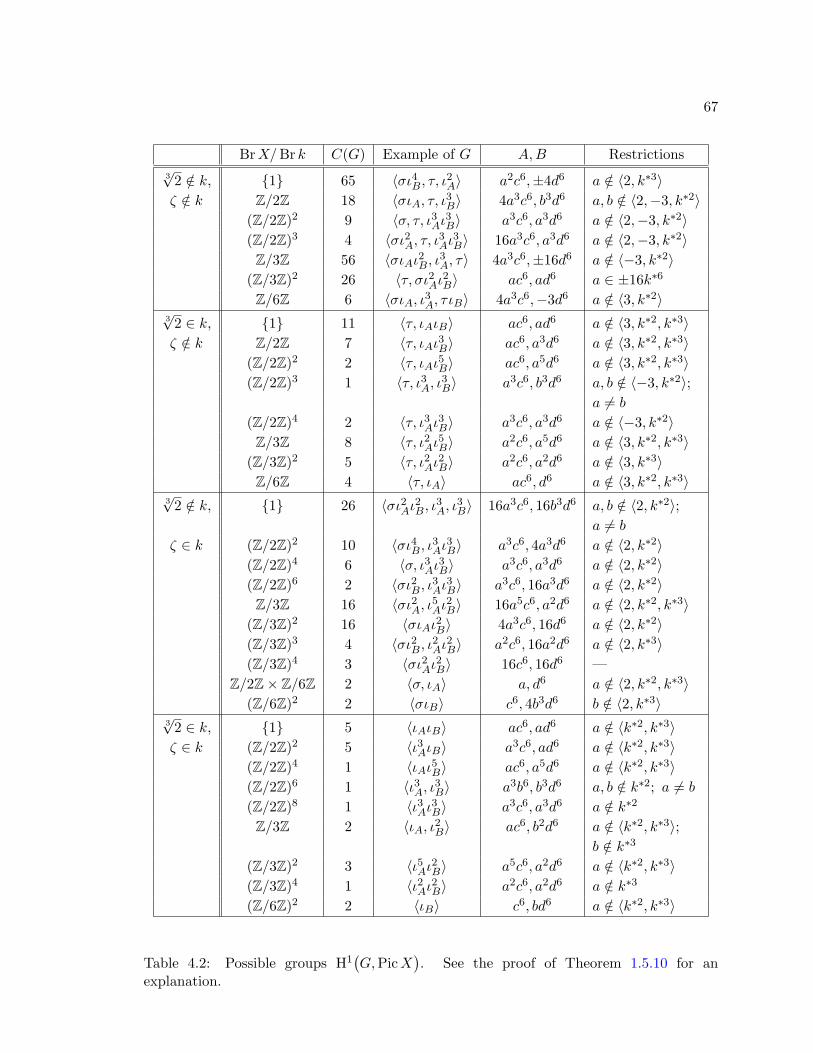
67

BrX/Br k C(G) Example of G A,B Restrictions3√

2 /∈ k, 1 65 〈σι4B, τ, ι2A〉 a2c6,±4d6 a /∈ 〈2, k∗3〉ζ /∈ k Z/2Z 18 〈σιA, τ, ι3B〉 4a3c6, b3d6 a, b /∈ 〈2,−3, k∗2〉

(Z/2Z)2 9 〈σ, τ, ι3Aι3B〉 a3c6, a3d6 a /∈ 〈2,−3, k∗2〉(Z/2Z)3 4 〈σι2A, τ, ι3Aι3B〉 16a3c6, a3d6 a /∈ 〈2,−3, k∗2〉Z/3Z 56 〈σιAι2B, ι3A, τ〉 4a3c6,±16d6 a /∈ 〈−3, k∗2〉

(Z/3Z)2 26 〈τ, σι2Aι2B〉 ac6, ad6 a ∈ ±16k∗6

Z/6Z 6 〈σιA, ι3A, τ ιB〉 4a3c6,−3d6 a /∈ 〈3, k∗2〉3√

2 ∈ k, 1 11 〈τ, ιAιB〉 ac6, ad6 a /∈ 〈3, k∗2, k∗3〉ζ /∈ k Z/2Z 7 〈τ, ιAι3B〉 ac6, a3d6 a /∈ 〈3, k∗2, k∗3〉

(Z/2Z)2 2 〈τ, ιAι5B〉 ac6, a5d6 a /∈ 〈3, k∗2, k∗3〉(Z/2Z)3 1 〈τ, ι3A, ι3B〉 a3c6, b3d6 a, b /∈ 〈−3, k∗2〉;

a 6= b

(Z/2Z)4 2 〈τ, ι3Aι3B〉 a3c6, a3d6 a /∈ 〈−3, k∗2〉Z/3Z 8 〈τ, ι2Aι5B〉 a2c6, a5d6 a /∈ 〈3, k∗2, k∗3〉

(Z/3Z)2 5 〈τ, ι2Aι2B〉 a2c6, a2d6 a /∈ 〈3, k∗3〉Z/6Z 4 〈τ, ιA〉 ac6, d6 a /∈ 〈3, k∗2, k∗3〉

3√

2 /∈ k, 1 26 〈σι2Aι2B, ι3A, ι3B〉 16a3c6, 16b3d6 a, b /∈ 〈2, k∗2〉;a 6= b

ζ ∈ k (Z/2Z)2 10 〈σι4B, ι3Aι3B〉 a3c6, 4a3d6 a /∈ 〈2, k∗2〉(Z/2Z)4 6 〈σ, ι3Aι3B〉 a3c6, a3d6 a /∈ 〈2, k∗2〉(Z/2Z)6 2 〈σι2B, ι3Aι3B〉 a3c6, 16a3d6 a /∈ 〈2, k∗2〉Z/3Z 16 〈σι2A, ι5Aι2B〉 16a5c6, a2d6 a /∈ 〈2, k∗2, k∗3〉

(Z/3Z)2 16 〈σιAι2B〉 4a3c6, 16d6 a /∈ 〈2, k∗2〉(Z/3Z)3 4 〈σι2B, ι2Aι2B〉 a2c6, 16a2d6 a /∈ 〈2, k∗3〉(Z/3Z)4 3 〈σι2Aι2B〉 16c6, 16d6 —

Z/2Z× Z/6Z 2 〈σ, ιA〉 a, d6 a /∈ 〈2, k∗2, k∗3〉(Z/6Z)2 2 〈σιB〉 c6, 4b3d6 b /∈ 〈2, k∗3〉

3√

2 ∈ k, 1 5 〈ιAιB〉 ac6, ad6 a /∈ 〈k∗2, k∗3〉ζ ∈ k (Z/2Z)2 5 〈ι3AιB〉 a3c6, ad6 a /∈ 〈k∗2, k∗3〉

(Z/2Z)4 1 〈ιAι5B〉 ac6, a5d6 a /∈ 〈k∗2, k∗3〉(Z/2Z)6 1 〈ι3A, ι3B〉 a3b6, b3d6 a, b /∈ k∗2; a 6= b

(Z/2Z)8 1 〈ι3Aι3B〉 a3c6, a3d6 a /∈ k∗2

Z/3Z 2 〈ιA, ι2B〉 ac6, b2d6 a /∈ 〈k∗2, k∗3〉;b /∈ k∗3

(Z/3Z)2 3 〈ι5Aι2B〉 a5c6, a2d6 a /∈ 〈k∗2, k∗3〉(Z/3Z)4 1 〈ι2Aι2B〉 a2c6, a2d6 a /∈ k∗3

(Z/6Z)2 2 〈ιB〉 c6, bd6 a /∈ 〈k∗2, k∗3〉

Table 4.2: Possible groups H1(G,PicX

). See the proof of Theorem 1.5.10 for an

explanation.

68

4.4 Finding cyclic algebras in BrX

Having computed the group H1(

Gal(ks/k,PicXks))

for diagonal del Pezzo sur-

faces of degree 1, it will be important for us to invert, as best we can, the isomorphism

BrX/Br k ∼−→ H1(

Gal(ks/k),PicXks)

furnished by the Hochschild-Serre spectral sequence; see §2.3.4. This problem is quite

hard in general. Instead, we present a simple strategy to search for cohomology classes

in H1(

Gal(ks/k),PicXks)

which correspond to cyclic algebras in the image of the natural

map

BrX/Br k → Br k(X)/Br k, (4.4)

where X is a locally soluble smooth geometrically integral variety over a number field k.

We are interested in cyclic algebras because their local invariants are relatively easy to

compute. We note that the map 4.4 is injective whenever X is a regular, integral, quasi-

compact scheme and X(Ak) 6= ∅; see [Mil80, III.2.22].

4.4.1 Review of cyclic algebras

Let L/k be a finite cyclic degree-n extension of fields. Fix a generator σ of

Gal(L/k). Let L[x]σ be the “twisted” polynomial ring, where `x = xσ(`) for all ` ∈ L.

Given b ∈ k∗, we construct the central simple k-algebra L[x]σ/(xn− b). This algebra is usu-

ally denoted (L/k, b); it depends on the choice of σ, though the notation does not show this.

If X is a geometrically integral k-variety, then the cyclic algebra (k(XL)/k(X), f) is also

denoted (L/k, f); this should not cause confusion because Gal(k(XL)/k(X)) ∼= Gal(L/k).

For a smooth variety X over a global field k, and a Galois extension L/k, we

write NL/k : DivXL → DivXk and NL/k : PicXL → PicXk for the usual norm maps,

respectively. The following is a criterion for testing whether or not a cyclic algebra is in the

image of the map BrX → Br k(X). For a proof, see [Cor05, Prop. 2.2.3] or [Bri02, Prop.

4.17].

Proposition 4.4.1. Let X be a smooth, geometrically integral variety over a field k. Let

L/k a finite cyclic extension and f ∈ k(X)∗. Then the cyclic algebra (L/k, f) is in the image

of the natural map Br(X)→ Br k(X) if and only if (f) = NL/k(D), for some D ∈ DivXL.

If, furthermore, X is locally soluble, then (L/k, f) comes from Br k if and only if we can

take D to be principal.

69

4.4.2 Cyclic Azumaya algebras

Let X be a smooth geometrically integral variety over a global field k. Assume

that X is locally soluble, and let L/k be a cyclic extension. Define the set

Brcyc(X,L) :=

classes [(L/k, f)] in the image of themap BrX/Br k → Br k(X)/Br k

Lemma 4.4.2. Viewing ∆ := 1 − σ as an endomorphism of DivXL, we have kerNL/k =

im ∆.

Proof. By Tate cohomology we know that H1(

Gal(L/k),DivXL

) ∼= kerNL/k/ im ∆. On

the other hand, this cohomology group is trivial: DivXL is a permutation module, so the

result follows from Shapiro’s Lemma.

The seeds behind the following theorem can already be found in [Bri02, §4.3.2,

especially Lemma 4.18].

Theorem 4.4.3. Let X be a k-variety as above. Let L/k be a cyclic degree-n extension,

generated by σ, and view ∆ = 1− σ as an endomorphism of PicXL. The map

ψ : kerNL/k/ im ∆→ Brcyc(X,L) [D] 7→ [(L/k, f)],

where f ∈ k(X)∗ is any function such that NL/k(D) = (f), is a group isomorphism.

Proof. First we check that ψ is well-defined by showing that

(i) the class [(L/k, f)] is independent of the choice of f : if NL/k(D) = (f) = (g), then

g = af for some a ∈ k∗. Since (L/k, a) ∈ Br k, we obtain [(L/k, f)] = [(L/k, g)].

(ii) if D and D′ are linearly equivalent divisors in kerNL/k, with NL/k(D) = (f) and

NL/k(D′) = (f ′), then [(L/k, f)] = [(L/k, f ′)]: Suppose that D = D′ + (h). Then

(f/f ′) = NL/k((h)), and by Proposition 4.4.1, we have (L/k, f/f ′) ∈ Br(k).

(iii) an element in im ∆ maps to zero: by (ii) it suffices to assume that D is of the form

E − σE. Then NL/k(D) = 0, so we can take f ∈ k∗ in the definition of ψ, in which

case (L/k, f) ∈ Br(k).

If NL/k(D) = (f) and NL/k(D′) = (g) then

ψ([D] + [D′]) = ψ([D +D′]) = [(L/k, fg)]

= [(L/k, f)] + [(L/k, g)] = ψ([D]) + ψ([D′]),(4.5)

70

so ψ is a homomorphism. The map ψ is injective: if ψ([D]) = [(L/k, f)] is 0 in Br k(X)/Br k,

then by Proposition 4.4.1 there exists an h ∈ k(XL)∗ such that (f) = NL/k((h)). Hence D−(h) ∈ kerNL/k = im ∆ (see Lemma 4.4.2). Surjectivity also follows from Proposition 4.4.1:

given a class [(L/k, f)], take any divisor D such that NL/k(D) = (f); then ψ([D]) =

[(L/k, f)].

4.4.3 Cyclic algebras on rational surfaces

Let X be a nice locally soluble rational surface over a global field k, and let K be

the splitting field of X. We saw in §2.3.4 that there exist isomorphisms

H1(

Gal(K/k),PicXK

) inf−→ H1(Gal(ks/k),PicXks

) ∼←− BrX/Br k, (4.6)

where the map on the right comes from the Hochschild-Serre spectral sequence.

Let G = Gal(K/k) and suppose that H is a normal subgroup of G such that G/H

is cyclic. Let L be the fixed field of H. Since (PicXK)H ∼= PicXL (by (2.14)), we obtain

an injection

H1(

Gal(L/k),PicXL

) inf−→ H1(G,PicXK

) ∼= BrX/Br k. (4.7)

On the other hand, by Tate cohomology we know that

H1(

Gal(L/k),PicXL

) ∼= kerNL/k/ im ∆.

We can thus use Theorem 4.4.3 to write down cyclic algebras (L/k, f) in the image of the

injection BrX/Br k → Br k(X)/Br k. Indeed, since G is finite, we may search through its

subgroup lattice to find subgroups H as above, and hence write down all cyclic algebras

coming from cyclic extensions of k (contained in K) in BrX/Br k. In summary, for each

H we consider the diagram

BrX/Br k ∼ //_

H1(

Gal(ks/k),PicXks)

Br k(X)/Br k H1(

Gal(K/k),PicXK

)inf ∼OO

H1(

Gal(L/k),PicXL

)?inf

OO

∼

Brcyc(X,L)?

OO

kerNL/k/ im ∆ψ

∼oo

71

and we construct elements of BrX/Br k by making the map ψ explicit. We believe the

above diagram commutes (perhaps up to sign), but have not checked this, and we do not

require to know this.

Remark 4.4.4. Finding Brauer-Manin obstructions to the Hasse principle on del Pezzo

surfaces of degree greater than 1 may require the injection (4.7) to be an isomorphism.

(This will be the case, for example, if H1(H,PicXK

)= 0). We may need representative

Azumaya algebras for every class in BrX/Br k to detect a Brauer-Manin obstruction (for

example, see [Cor07, 9.4]). Obstructions to weak approximation require only one Azumaya

algebra.

Remark 4.4.5. LetX be a diagonal del Pezzo surface of degree 1 overQ such that the order of

BrX/BrQ is divisible by 3. Let K be the splitting field of X. Then an exhaustive computer

search reveals that there does not exist a normal subgroup H of G := Gal(K/Q) such that

|G/H| is divisible by 3. This means that any counterexamples to weak approximation over

Q we find using the above strategy will always arise from 2-torsion Azumaya algebras.

Remark 4.4.6. Not all Brauer-Manin obstructions on del Pezzo surfaces arise from cyclic

algebras: for example, see [KT04, Example 8].

4.5 Counterexamples to Weak Approximation

4.5.1 A warm-up example

Let ζ be a primitive third root of unity. We begin with an counterexample to

weak approximation over k = Q(ζ) for which we do not need to use the descent procedure

described in §2.3.5, and for which Gal(K/k) is small. The presence of an obstruction to

weak approximation on it cannot be explained by a standard conic bundle structure (see

Remark 4.5.2).

Proposition 4.5.1. Let X be the del Pezzo surface of degree 1 over k = Q(ζ) given by

w2 = z3 + 16x6 + 16y6

in Pk(1, 1, 2, 3). Then X is k-minimal and there is a Brauer-Manin obstruction to weak

approximation on X. The obstruction arises from a cyclic algebra class in BrX/Br k.

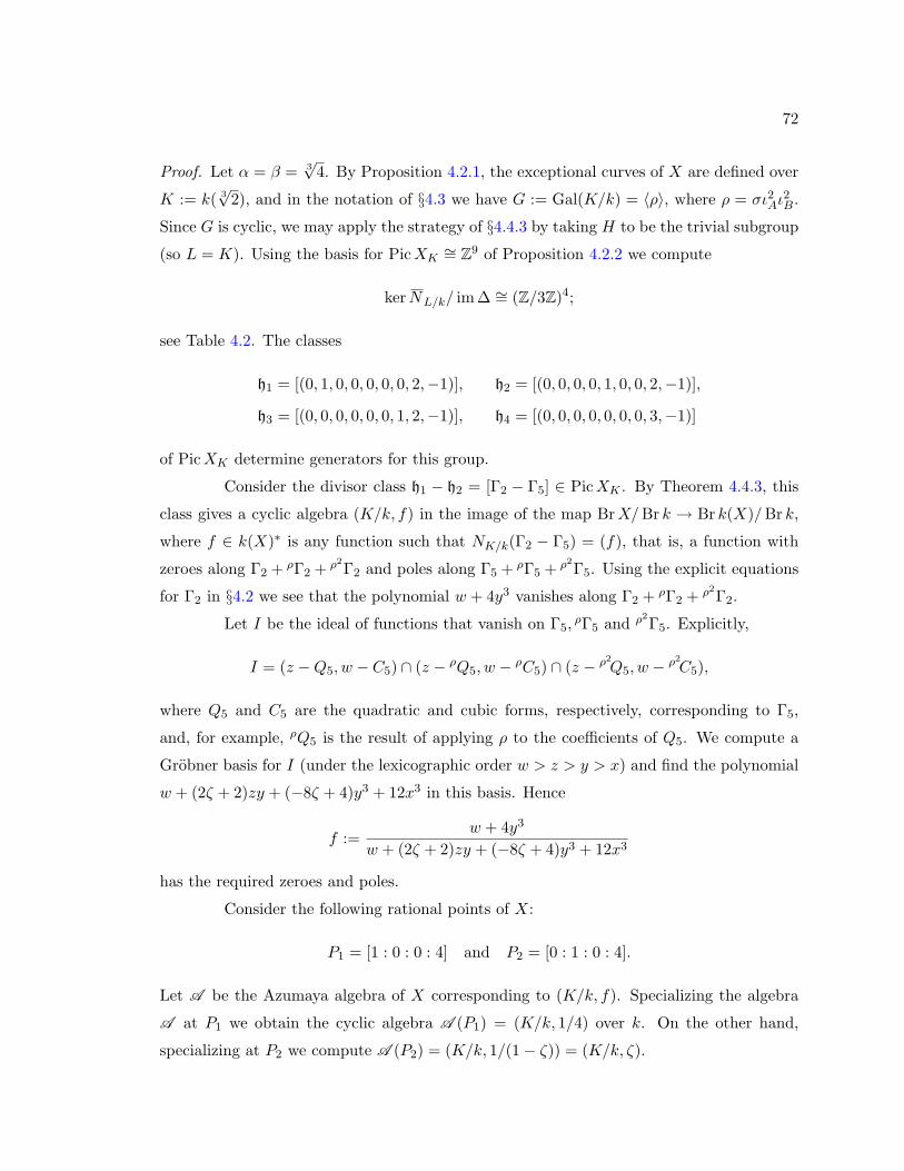
72

Proof. Let α = β = 3√

4. By Proposition 4.2.1, the exceptional curves of X are defined over

K := k( 3√

2), and in the notation of §4.3 we have G := Gal(K/k) = 〈ρ〉, where ρ = σι2Aι2B.

Since G is cyclic, we may apply the strategy of §4.4.3 by taking H to be the trivial subgroup

(so L = K). Using the basis for PicXK∼= Z9 of Proposition 4.2.2 we compute

kerNL/k/ im ∆ ∼= (Z/3Z)4;

see Table 4.2. The classes

h1 = [(0, 1, 0, 0, 0, 0, 0, 2,−1)], h2 = [(0, 0, 0, 0, 1, 0, 0, 2,−1)],

h3 = [(0, 0, 0, 0, 0, 0, 1, 2,−1)], h4 = [(0, 0, 0, 0, 0, 0, 0, 3,−1)]

of PicXK determine generators for this group.

Consider the divisor class h1 − h2 = [Γ2 − Γ5] ∈ PicXK . By Theorem 4.4.3, this

class gives a cyclic algebra (K/k, f) in the image of the map BrX/Br k → Br k(X)/Br k,

where f ∈ k(X)∗ is any function such that NK/k(Γ2 − Γ5) = (f), that is, a function with

zeroes along Γ2 + ρΓ2 + ρ2Γ2 and poles along Γ5 + ρΓ5 + ρ2Γ5. Using the explicit equations

for Γ2 in §4.2 we see that the polynomial w + 4y3 vanishes along Γ2 + ρΓ2 + ρ2Γ2.

Let I be the ideal of functions that vanish on Γ5,ρΓ5 and ρ2Γ5. Explicitly,

I = (z −Q5, w − C5) ∩ (z − ρQ5, w − ρC5) ∩ (z − ρ2Q5, w − ρ2C5),

where Q5 and C5 are the quadratic and cubic forms, respectively, corresponding to Γ5,

and, for example, ρQ5 is the result of applying ρ to the coefficients of Q5. We compute a

Grobner basis for I (under the lexicographic order w > z > y > x) and find the polynomial

w + (2ζ + 2)zy + (−8ζ + 4)y3 + 12x3 in this basis. Hence

f :=w + 4y3

w + (2ζ + 2)zy + (−8ζ + 4)y3 + 12x3

has the required zeroes and poles.

Consider the following rational points of X:

P1 = [1 : 0 : 0 : 4] and P2 = [0 : 1 : 0 : 4].

Let A be the Azumaya algebra of X corresponding to (K/k, f). Specializing the algebra

A at P1 we obtain the cyclic algebra A (P1) = (K/k, 1/4) over k. On the other hand,

specializing at P2 we compute A (P2) = (K/k, 1/(1− ζ)) = (K/k, ζ).

73

Let p be the unique prime above 3 in k. To compute the invariants we observe

that

invp(A (Pi)) =13

[f(Pi), 2]p ∈ Q/Z,

where [f(Pi)p, 2]p ∈ Z/3Z is the (additive) norm residue symbol. We compute [1/4, 2]p ≡0 mod 3 (using [CTKS87, (77)]) and [ζ, 2]p ≡ 1 mod 3 (using biadditivity of the norm residue

symbol and [CTKS87, (75)] with θ = −ζ, a = 1). Let P ∈ X(Ak) be the point that is equal

to P1 at all places except p, and is P2 at p. Then∑v

invv(A (Pv)) = 1/3,

so P ∈ X(Ak) \X(Ak)Br and X is a counterexample to weak approximation.

To see that X is k-minimal, see the proof of Theorem 1.5.10: the surface X appears

as the example in the twelfth line from the bottom of Table 4.2.

Remark 4.5.2. The surface X of Proposition 4.5.1 is not birational to a conic bundle C,

since the birational invariant BrX/Br k is isomorphic to (Z/3Z)4, while BrC/Br k is always

2-torsion. In particular, the failure of weak approximation cannot be accounted for by the

presence of a rational conic bundle structure.

4.5.2 Main Counterexamples

Proof of Theorem 1.5.7. Let α = β =√p. By Proposition 4.2.1, the exceptional curves ofX

are defined over K := Q(ζ, 3√

2,√p), and in the notation of §4.3 we have G := Gal(K/Q) =

〈σ, τ, ι3Aι3B〉. One easily checks that the element ρ := ι3Aι3B acts on exceptional curves as the

Bertini involution of the surface (see §4.1.1).

The subgroup H := 〈σ, τ〉 of G has index 2; hence it is normal and G/H is cyclic.

Thus, we are in the situation described in §4.4.3, that is,

H1(Gal(L/Q),PicXL) → BrX/BrQ,

where L = KH is Q(√p) in this case. The injection is in fact an isomorphism because

H1(H,PicXK) = 0, though we will not use this fact1. Using the basis for PicXK∼= Z9 of

Proposition 4.2.2 we compute

kerNL/k/ im ∆ ∼= Z/2Z× Z/2Z.1The isomorphism follows from the inflation-restriction exact sequence and (4.7).

74

The classes

h1 = [(2, 1, 1, 1, 1, 0, 1, 2,−3)] and h2 = [(0, 0, 0, 0, 0, 1, 0,−1, 0)] (4.8)

of PicXL generate this group. In fact, PicXL∼= Z3, generated by the classes (4.8) and the

anticanonical class, and ρ interchanges the classes (4.8). It follows that (PicXL)Gal(L/Q) =

Z, generated by the anticanonical class. By (2.14), we obtain PicX ∼= Z, and thus X is

minimal.

Next, we apply the procedure of §2.3.5 to descend the line bundle OXK (Γ6 − Γ8)

in the class of h2 to a line bundle defined over Q(√p). We must give isomorphisms

fh : OXK (Γ6 − Γ8)→ OXK (hΓ6 − hΓ8),

one for each h ∈ H, satisfying the cocycle condition. In this case H is isomorphic to the

symmetric group on 3 elements, with presentation

H = 〈σ, τ |σ3 = τ2 = 1, στ = τσ2〉,

so it is enough to find isomorphisms fσ and fτ as above such that

σ2fσ σfσ fσ = id,

τfτ fτ = id,

σfτ fσ = τσfσ τfσ fτ .

For example, the map fσ is just multiplication by a function having zeroes at Γ6 and σΓ8

and poles at Γ8 and σΓ6. We also denote this function fσ, and find it as follows. First, take

a function that vanishes on Γ8, σΓ6, and possibly some extra lines. For example, recall that

Γ6 = V (z −Q6(x, y), w − C6(x, y)), and Γ8 = V (z −Q8(x, y), w − C8(x, y)),

where Q6 and Q8 (resp C6 and C8) are the quadratic (resp. cubic) forms in x and y,

corresponding to Γ6 and Γ8 given in §4.2. Let σQ6 denote the result of applying σ to the

coefficients of Q6, and similarly for the other binary and cubic forms. The function

g1 = (z − σQ6(x, y))(z −Q8(x, y))

vanishes on the exceptional curves2 σΓ6, σΓ′6, Γ8 and Γ′8. Let I be the ideal of functions

that vanish on Γ6, σΓ8, σΓ′6 and Γ′8. Explicitly,

I = (z −Q6, w − C6) ∩ (z − σQ8, w − σC8) ∩ (z − σQ6, w + σC6) ∩ (z −Q8, w + C8).2The notation σΓ′6 is unambiguous (cf. Remark 4.1.6).

75

We compute a Grobner basis for I (under the lexicographic order w > z > y > x) and find

the following degree 4 polynomial in the basis:

f1 = 6√pwy + 3

√p(ζ − 1)(s2 + 2)wx+ (−2ζ + 1)sz2 + 2p(2ζ − 1)(s2 + s+ 1)zy2

+ p(−ζ − 1)(3s2 + 2s+ 2)zyx+ 2p(−ζ + 2)(s2 + s+ 1)zx2 + 2p2(2ζ − 1)(s2 + 1)y4

+ p2(−ζ − 1)(3s2 + 2s+ 2)y3x+ 2p2(−ζ + 2)(s2 + s+ 1)y2x2

+ 2p2(2ζ − 1)(s+ 1)yx3 + p2(ζ + 1)(s2 − 2)x4.

The function f1/g1 has the right zeroes and poles to be fσ. We set

fσ :=1

(−2ζ + 1)s· f1

g1.

The constant in front of f1/g1 is a normalization factor, making fσ([0 : 0 : 1 : 1]) = 1.

Similarly, fτ denotes a function with zeroes at Γ6 and τΓ8 and poles at Γ8 andτΓ6. Let

g2 = (z − τQ6(x, y))(z −Q8(x, y)),

f2 = 6√pwy −√pwx+ (−2ζ + 1)kz2 + 2p(2ζ − 1)(k2 + k + 1)zy2

+ 2p(2ζ − 1)(k + 1)zyx+ 2p(2ζ − 1)(k2 + k + 1)zx2 + 2p2(2ζ − 1)(k2 + 1)y4

+ 2p2(2ζ − 1)(k + 1)y3x+ 2p2(2ζ − 1)(k2 + k + 1)y2x2 + 2p2(2ζ − 1)(k + 1)yx3

+ 2p2(2ζ − 1)(k2 + 1)x4.

Then the function

fτ :=1

(−2ζ + 1)k· f2

g2

has zeroes at Γ6 and τΓ8 and poles at Γ8 and τΓ6. Because of the normalization, fτ and fσ

satisfy the cocycle condition. Thus OXK (Γ6 − Γ8) descends to a line bundle F over L, as

we expected. It remains to find a divisor over L in the class of F . To this end, we average

the rational section 1 of OXK (Γ6 − Γ8) over the group H to obtain a rational section

s =∑h∈H

h−1(fh) = 1 + σ2

fσ + τfτ + σ2fσ · σfσ + σ2

fσ · σfσ · στfτ + σ2fσ · τσfτ

of F . The common denominator of s is

σ2g1 · τg2 · σg1 · στg2 · τσg2.

76

By definition of g1 and g2 this denominator vanishes along the divisor

2Γ6 + 2Γ′6 + σ2Γ8 + σ2

Γ′8 + τΓ8 + τΓ′8 + 2(σ2

Γ6

)+ 2(σ2

Γ′6)

+ σΓ8 + σΓ′8 + στΓ8 + στΓ′8 + σΓ6 + σΓ′6 + τσΓ8 + τσΓ′8.

Here 2Γ6 means, for example, that the denominator vanishes on this curve to order 2. The

numerator of s vanishes along the divisor

Γ6 + 2Γ′6 + σ2Γ′8 + τΓ′8 + 2

(σ2

Γ6

)+ 2(σ2

Γ′6)

+ σΓ′8 + στΓ′8 + σΓ6 + σΓ′6 + τσΓ′8 + Z,

where Z is some curve on XL. Thus, the divisor of s as a rational function is Z −P , where

P := Γ6 + σ2Γ8 + τΓ8 + στΓ8 + σΓ8 + τσΓ8

The divisor of s as a rational section of OXK (Γ6 − Γ8), is (Z − P )− (Γ6 − Γ8). Let

P ′ := Γ8 + σ2Γ8 + τΓ8 + στΓ8 + σΓ8 + τσΓ8 =

∑h∈H

hΓ8;

the divisor Z − P ′ ∈ DivXL represents the class of Γ6 − Γ8.

Let ρ be the image of ρ in Gal(L/Q). By Theorem 4.4.3, the class [Z − P ′] gives

a cyclic algebra (Q(√p)/Q, f) in BrX/BrQ, where f ∈ Q(X)∗ is any function such that

NQ(√p)/Q(Z − P ′) = Z + ρZ − (P ′ + ρP ′) = (f).

We find an explicit f . The numerator of s (after cancelling out common divisors)

is a polynomial of degree 12 in Q( 3√

2, ζ,√p)[x, y, z, w]. We may express it as

p1 + 3√

2p2 + 3√

4p3 + ζp4 + ζ3√

2p5 + ζ3√

4p6,

where pi ∈ Q(√p)[x, y, z, w] for i = 1, . . . , 6. Then Z = V (p1, . . . , p6). We find constants

bi ∈ Q(√p) such that the polynomial q =

∑i bipi belongs to Q[x, y, z, w]; then the polyno-

mial q vanishes on Z ∪ ρZ and is a suitable numerator for f . A little linear algebra reveals

77

that

q = 12z6 − 72pz5y2 − 192pz5yx− 48pz5x2 + 300p2z4y4 + 600p2z4y3x+ 576p2z4y2x2

+ 408p2z4yx3 + 156p2z4x4 − 288p3z3y6 − 720p3z3y5x− 888p3z3y4x2 − 768p3z3y3x3

− 756p3z3y2x4 − 264p3z3yx5 − 204p3z3x6 + 144p4z2y8 + 456p4z2y7x

+ 1032p4z2y6x2 + 1080p4z2y5x3 + 756p4z2y4x4 + 864p4z2y3x5 + 684p4z2y2x6

+ 456p4z2yx7 − 48p4z2x8 + 192p5zy10 − 48p5zy9x− 720p5zy8x2 − 1104p5zy7x3

− 600p5zy6x4 − 216p5zy5x5 − 240p5zy4x6 − 480p5zy3x7 − 504p5zy2x8 − 24p5zyx9

+ 48p5zx10 − 192p6y12 − 288p6y11x+ 192p6y10x2 + 528p6y9x3 + 432p6y8x4

+ 168p6y7x5 − 192p6y6x6 − 288p6y5x7 + 192p6y4x8 + 312p6y3x9 − 48p6yx11

works. Now we look for a polynomial r of the same degree as q vanishing on P ′+ ρP ′. Since

ρ acts as the Bertini involution Γ 7→ Γ′ on exceptional curves, we have

P ′ + ρP ′ =∑h∈H

h(Γ8 + Γ′8).

The polynomial z −Q8(x, y) vanishes on Γ8 + Γ′8. Hence we may take

r =∏h∈H

(z − hQ8(x, y)),

and obtain

r = z6 − 6pz5y2 − 24pz5yx− 6pz5x2 + 36p2z4y4 + 78p2z4y3x+ 132p2z4y2x2

+ 78p2z4yx3 + 36p2z4x4 + 8p3z3y6 − 60p3z3y5x− 168p3z3y4x2 − 276p3z3y3x3

− 168p3z3y2x4 − 60p3z3yx5 + 8p3z3x6 − 24p4z2y8 − 24p4z2y7x+ 156p4z2y6x2

+ 396p4z2y5x3 + 540p4z2y4x4 + 396p4z2y3x5 + 156p4z2y2x6 − 24p4z2yx7

− 24p4z2x8 + 24p5zy9x+ 24p5zy8x2 − 120p5zy7x3 − 324p5zy6x4 − 432p5zy5x5

− 324p5zy4x6 − 120p5zy3x7 + 24p5zy2x8 + 24p5zyx9 + 16p6y12 + 48p6y11x

+ 48p6y10x2 + 48p6y9x3 + 120p6y8x4 + 192p6y7x5 + 212p6y6x6 + 192p6y5x7

+ 120p6y4x8 + 48p6y3x9 + 48p6y2x10 + 48p6yx11 + 16p6x12.

Let f = q/r and let A denote the Azumaya algebra on X corresponding to (L/Q, f). There

are two obvious rational points on the surface X other than the anticanonical point, namely,

P1 = [1 : 0 : −p : 0] and P2 = [0 : 1 : −p : 0].

78

Specializing the algebra A at P1 we obtain the quaternion algebra (p, 12) ∼= (p, 3) over Q.

The invariant of this algebra at a prime q is calculated using the Hilbert symbol [ · , · ]q ∈±1 of the quaternion algebra: the invariant is 0 if the Hilbert symbol is +1 and 1/2 if the

Hilbert symbol is −1. Using the formulas for the Hilbert symbol in [Ser73], we find that

[p, 3]q =

(−1)(p−1)/2 if q = 2,(p

3

)if q = 3,(

3p

)if q = p,

1 otherwise,

where(p

q

)is the usual Legendre symbol. On the other hand, specializing A at P2 we

obtain the quaternion algebra (p, 16) ∼= (p, 1) over Q. We find that [p, 1]q = 1 for all primes

q. Hence

inv3(p, 3) 6= inv3(p, 1) if p ≡ 5 mod 6 and inv2(p, 3) 6= inv2(p, 1) if p ≡ 3 mod 4. (4.9)

Let P ∈ X(AQ) be the point that is equal to P1 at all places except p, and is P2 at p. Then

by (4.9) it follows that if p ≡ 5 mod 6 then∑v

invv(A (Pv)) = 1/2.

Similarly, if P ′ ∈ X(AQ) is the point that is equal to P1 at all places except 2, and is P2 at

2, then by (4.9) we find that the sum of invariants is again 1/2 when p ≡ 3 mod 4.

If p > 3 is a prime such that p 6≡ 1 mod 12, then either p ≡ 3 mod 4 or p ≡ 5 mod 6,

and by our computations above it follows that X(AQ) 6= X(AQ)Br. We conclude that X

does not satisfy weak approximation.

79

Bibliography

[BSD75] B. J. Birch and H. P. F. Swinnerton-Dyer, The Hasse problem for rational surfaces, J. Reine

Angew. Math. 274/275 (1975), 164–174. ↑1.4.3, 1.4

[BLR90] S. Bosch, W. Lutkebohmert, and M. Raynaud, Neron models, Ergebnisse der Mathematik und

ihrer Grenzgebiete (3), vol. 21, Springer, Berlin, 1990. ↑2.3.5

[BCP97] W. Bosma, J. Cannon, and C. Playoust, The Magma algebra system. I. The user language, J.

Symbolic Comput. 24 (1997), no. 3-4, 235–265. ↑4

[Bri02] M. Bright, Computations on diagonal quartic surfaces, Cambridge University, 2002. Ph. D.

Thesis. ↑4.4.1, 4.4.2

[CG66] J. W. S. Cassels and M. J. T. Guy, On the Hasse principle for cubic surfaces, Mathematika

13 (1966), 111–120. ↑1.4.2, 1.4

[Cha44] F. Chatelet, Variations sur un theme de H. Poincare, Ann. Sci. Ecole Norm. Sup. (3) 61

(1944), 249–300 (French). ↑1.4

[CT72a] J.-L. Colliot-Thelene, Surfaces de Del Pezzo de degre 6, C. R. Acad. Sci. Paris Ser. A-B 275

(1972), A109–A111 (French). ↑1.4

[CT72b] , Quelques proprietes arithmetiques des surfaces rationnelles, Seminaire de Theorie des

Nombres, 1971–1972 (Univ. Bordeaux I, Talence), Exp. No. 13, Lab. Theorie des Nombres,

Centre Nat. Recherche Sci., Talence, 1972, pp. 22. ↑1.4

[CT03] , Points rationnels sur les fibrations, Higher dimensional varieties and rational points

(Budapest, 2001), Bolyai Soc. Math. Stud., vol. 12, Springer, Berlin, 2003, pp. 171–221

(French). ↑2.3.3

[CTCS80] J.-L. Colliot-Thelene, D. Coray, and J.-J. Sansuc, Descente et principe de Hasse pour certaines

varietes rationnelles, J. Reine Angew. Math. 320 (1980), 150–191 (French). ↑1.2, 2.3.3

[CTKS87] J.-L. Colliot-Thelene, D. Kanevsky, and J.-J. Sansuc, Arithmetique des surfaces cubiques di-

agonales, Diophantine approximation and transcendence theory, 1987, pp. 1–108. ↑2.3.3, 4.5.1

[CTS80] J.-L. Colliot-Thelene and J.-J. Sansuc, La descente sur les varietes rationnelles, Journees de

Geometrie Algebrique d’Angers, Juillet 1979, Sijthoff & Noordhoff, Alphen aan den Rijn, 1980,

pp. 223–237. ↑2.3.3

80

[CTS82] , Sur le principe de Hasse et l’approximation faible, et sur une hypothese de Schinzel,

Acta Arith. 41 (1982), no. 1, 33–53. ↑2.3.3

[CTSSD87a] J.-L. Colliot-Thelene, J.-J. Sansuc, and H. P. F. Swinnerton-Dyer, Intersections of two quadrics

and Chatelet surfaces. I, J. Reine Angew. Math. 373 (1987), 37–107. ↑1.4

[CTSSD87b] , Intersections of two quadrics and Chatelet surfaces, J. Reine Angew. Math. 374 (1987),

72–168. ↑1.4, 1.4.9, 1.4

[CTSSD98] J.-L. Colliot-Thelene, A. N. Skorobogatov, and H. P. F. Swinnerton-Dyer, Hasse principle for

pencils of curves of genus one whose Jacobians have rational 2-division points, Invent. Math.

134 (1998), no. 3, 579–650. ↑3.5

[Coo88] K. R. Coombes, Every rational surface is separably split, Comment. Math. Helv. 63 (1988),

no. 2, 305–311. ↑2.1.2, 2.1.3

[Cor05] P. Corn, Del Pezzo surfaces and the Brauer-Manin obstruction, University of California, Berke-

ley, 2005. Ph. D. Thesis. ↑2.3.3, 4.4.1

[Cor07] , The Brauer-Manin obstruction on del Pezzo surfaces of degree 2, Proc. London Math.

Soc. (3) 95 (2007), no. 3, 735–777. ↑1.5.11, 4.3.1, 4.4.4

[CO99] P. Cragnolini and P. A. Oliverio, Lines on del Pezzo surfaces with K2S = 1 in characteristic

6= 2, Comm. Algebra 27 (1999), no. 3, 1197–1206. ↑2.2.3, 2.2.3, 4.1.2, 4.1.5

[Deb01] Olivier Debarre, Higher-dimensional algebraic geometry, Universitext, Springer-Verlag, New

York, 2001. MR 1841091 (2002g:14001) ↑4.1.3

[dJ] A. J. de Jong, A result of Gabber. Preprint http://www.math.columbia.edu/˜dejong/ papers/2-

gabber.pdf. ↑2.3.1

[Del73] P. Deligne, Les constantes des equations fonctionnelles des fonctions L, Modular functions of

one variable, II (Proc. Internat. Summer School, Univ. Antwerp, Antwerp, 1972), Springer,

Berlin, 1973, pp. 501–597. Lecture Notes in Math., Vol. 349 (French). ↑3.1

[Dem80] M. Demazure, Surfaces de Del Pezzo II, III, IV, V, Seminaire sur les Singularites des Surfaces,

Lecture Notes in Mathematics, vol. 777, Springer, Berlin, 1980, pp. 23–69. ↑1.3, 1.4, 2.2, 4.1.1,

4.1.5

[DD07] T. Dokchitser and V. Dokchitser, On the Birch–Swinnerton-Dyer quotients modulo squares

(April 9, 2007). Preprint arxiv:math/0610290. ↑1.5.1, 3.1

[Enr97] F. Enriques, Sulle irrazionalita da cui puo farsi dipendere la risoluzione d’un’ equazione alge-

brica f(xyz) = 0 con funzioni razionali di due parametri, Math. Ann. 49 (1897), no. 1, 1–23

(Italian). ↑1.4

[Ful98] W. Fulton, Intersection theory, 2nd ed., Ergebnisse der Mathematik und ihrer Grenzgebiete.,

vol. 2, Springer-Verlag, Berlin, 1998. ↑4.2

[GM91] F. Gouvea and B. Mazur, The square-free sieve and the rank of elliptic curves, J. Amer. Math.

Soc. 4 (1991), no. 1, 1–23. ↑1.5.1, 3.2, 3.2.1, 3.2, 3.2

81

[GM97] G. R. Grant and E. Manduchi, Root numbers and algebraic points on elliptic surfaces with base

P1, Duke Math. J. 89 (1997), no. 3, 413–422. ↑1.5.1

[Gre92] G. Greaves, Power-free values of binary forms, Quart. J. Math. Oxford Ser. (2) 43 (1992),

no. 169, 45–65. ↑1.5.1, 3.2, 3.2

[Gro03] A. Grothendieck, Revetements etales et groupe fondamental (SGA 1), Documents

Mathematiques, 3, Societe Mathematique de France, Paris, 2003. ↑2.3.5

[Gro68a] , Le groupe de Brauer. I. Algebres d’Azumaya et interpretations diverses, Dix Exposes

sur la Cohomologie des Schemas, North-Holland, Amsterdam, 1968, pp. 46–66 (French). MR

0244269 (39 #5586a) ↑2.3.1

[Gro68b] , Le groupe de Brauer. III. Exemples et complements, Dix Exposes sur la Cohomologie

des Schemas, North-Holland, Amsterdam, 1968, pp. 88–188 (French). ↑2.3.8

[Hal98] E. Halberstadt, Signes locaux des courbes elliptiques en 2 et 3, C. R. Acad. Sci. Paris Ser. I

Math. 326 (1998), no. 9, 1047–1052 (French, with English and French summaries). ↑1.5.1, 3.1

[Har00] D. Harari, Weak approximation and non-abelian fundamental groups, Ann. Sci. Ecole Norm.

Sup. (4) 33 (2000), no. 4, 467–484 (English, with English and French summaries). ↑2.3.3

[Har04] , Weak approximation on algebraic varieties, Arithmetic of higher-dimensional algebraic

varieties (Palo Alto, CA, 2002), 2004, pp. 43–60. ↑2.3.11

[HS05] D. Harari and A. Skorobogatov, Non-abelian descent and the arithmetic of Enriques surfaces,

Int. Math. Res. Not. (2005), no. 52, 3203–3228. ↑2.3.3

[Har77] R. Hartshorne, Algebraic geometry, Springer-Verlag, New York, 1977. Graduate Texts in Math-

ematics, No. 52. ↑1.3, 2.2.1

[Has09] B. Hassett, Rational surfaces over nonclosed fields, to appear in the Proceedings of the 2006

Clay Summer School (2009). ↑1.3, 1.3, 1.3

[Isk67] V. A. Iskovskikh, Rational surfaces with a pencil of rational curves, Mat. Sb. (N.S.) 74 (116)

(1967), 608–638 (Russian). MR 0220734 (36 #3786) ↑1.4

[Isk71] , A counterexample to the Hasse principle for systems of two quadratic forms in five

variables, Mat. Zametki 10 (1971), 253–257 (Russian). MR 0286743 (44 #3952) ↑1.4.4

[Isk79] , Minimal models of rational surfaces over arbitrary fields, Izv. Akad. Nauk SSSR Ser.

Mat. 43 (1979), no. 1, 19–43, 237 (Russian). ↑1.2.3, 1.3.4

[IK04] Henryk Iwaniec and Emmanuel Kowalski, Analytic number theory, American Mathematical

Society Colloquium Publications, vol. 53, American Mathematical Society, Providence, RI,

2004. ↑3.2

[Kle05] Steven L. Kleiman, The Picard scheme, Fundamental algebraic geometry, Math. Surveys

Monogr., vol. 123, Amer. Math. Soc., Providence, RI, 2005, pp. 235–321. ↑1.3

[Kol96] J. Kollar, Rational curves on algebraic varieties, Ergebnisse der Mathematik und ihrer Gren-

zgebiete (3), vol. 32, Springer, Berlin, 1996. ↑2.2, 2.2.3, 2.2.3

82

[KT04] A. Kresch and Y. Tschinkel, On the arithmetic of del Pezzo surfaces of degree 2, Proc. London

Math. Soc. (3) 89 (2004), no. 3, 545–569. ↑1.4.1, 1.4, 1.5.2, 4.4.6

[KT06] , Effectivity of Brauer-Manin obstructions (December 21, 2006). Preprint

math/0612665. ↑2.3.5

[KT08] , Two examples of BrauerManin obstruction to integral points, Bull. London Math. Soc.

(May 21, 2008). To appear; doi:10.1112/blms/bdn081. ↑1.4.7, 1.4

[Lan54] S. Lang, Some applications of the local uniformization theorem, Amer. J. Math. 76 (1954),

362–374. ↑1.2

[Lin40] C.-E. Lind, Untersuchungen uber die rationalen Punkte der ebenen kubischen Kurven vom

Geschlecht Eins, Thesis, University of Uppsala, 1940 (1940), 97 (German). ↑1.1

[Liv95] E. Liverance, A formula for the root number of a family of elliptic curves, J. Number Theory

51 (1995), no. 2, 288–305. ↑3.1.3

[Man71] Y. I. Manin, Le groupe de Brauer-Grothendieck en geometrie diophantienne, Actes du Congres

International des Mathematiciens (Nice, 1970), Gauthier-Villars, Paris, 1971, pp. 401–411. ↑2.3

[Man74] Yu. I. Manin, Cubic forms: algebra, geometry, arithmetic, North-Holland Publishing Co., Am-

sterdam, 1974. ↑1.1, 1.4, 1.4.6, 1.5, 1.5.2, 2.1, 2.1.4, 2.2, 2.2.2, 2.2.2

[MT86] Yu. I. Manin and M. A. Tsfasman, Rational varieties: algebra, geometry, arithmetic, Uspekhi

Mat. Nauk 41 (1986), no. 2(248), 43–94 (Russian). English translation: Russian Math. Surveys

41 (1986), no. 2, 51–116. ↑1.3, 1.4

[Mil70] J. S. Milne, The Brauer group of a rational surface, Invent. Math. 11 (1970), 304–307. ↑2.3.1

[Mil80] , Etale cohomology, Princeton Mathematical Series, vol. 33, Princeton University Press,

Princeton, N.J., 1980. ↑2.3.1, 2.3.1, 4.4

[Nek01] J. Nekovar, On the parity of ranks of Selmer groups. II, C. R. Acad. Sci. Paris Ser. I Math.

332 (2001), no. 2, 99–104. ↑1.5.1, 3.1

[Neu99] J. Neukirch, Algebraic number theory, Grundlehren der Mathematischen Wissenschaften,

vol. 322, Springer-Verlag, Berlin, 1999. ↑3.3.1

[NSW08] J. Neukirch, A. Schmidt, and K. Wingberg, Cohomology of number fields, 2nd ed., Grundlehren

der Mathematischen Wissenschaften, vol. 323, Springer-Verlag, Berlin, 2008. ↑2.3.4

[Nis55] H. Nishimura, Some remarks on rational points, Mem. Coll. Sci. Univ. Kyoto. Ser. A. Math.

29 (1955), 189–192. ↑1.2

[Poo07] B. Poonen, Existence of rational points on smooth projective varieties (2007). to appear in J.

Europ. Math. Soc. ↑1.4

[Poo08] , Insufficiency of the Brauer-Manin obstruction applied to etale covers (August 10,

2008). Preprint math/0612665. ↑1.3, 2.3.3

[Rei42] H. Reichardt, Einige im Kleinen uberall losbare, im Grossen unlosbare diophantische Gleichun-

gen, J. Reine Angew. Math. 184 (1942), 12–18 (German). ↑1.1

83

[Riz03] O. G. Rizzo, Average root numbers for a nonconstant family of elliptic curves, Compositio

Math. 136 (2003), no. 1, 1–23. ↑1.5.1, 3.1, 3.1.1, 3.1.1, 3.1.2, 3.1.2

[Roh93] D. E. Rohrlich, Variation of the root number in families of elliptic curves, Compositio Math.

87 (1993), no. 2, 119–151. ↑1.5.1, 3.1, 3.1.4

[Sal88] P. Salberger, Zero-cycles on rational surfaces over number fields, Invent. Math. 91 (1988),

no. 3, 505–524. ↑1.4

[SS91] P. Salberger and A. N. Skorobogatov, Weak approximation for surfaces defined by two quadratic

forms, Duke Math. J. 63 (1991), no. 2, 517–536. ↑2.3.3

[Ser73] J.-P. Serre, A course in arithmetic, Graduate Texts in Mathematics, vol. 7, Springer, New

York, 1973. ↑4.5.2

[Ser88] Jean-Pierre Serre, Algebraic groups and class fields, Graduate Texts in Mathematics, vol. 117,

Springer-Verlag, New York, 1988. Translated from the French. MR 918564 (88i:14041) ↑1.3,

4.1.3

[Ser08] , Topics in Galois theory, 2nd ed., Research Notes in Mathematics, vol. 1, A K Peters

Ltd., Wellesley, MA, 2008. With notes by Henri Darmon. ↑2.3.14, 2.3.3

[SB92] N. I. Shepherd-Barron, The rationality of quintic Del Pezzo surfaces—a short proof, Bull.

London Math. Soc. 24 (1992), no. 3, 249–250. ↑1.4

[Shi90] T. Shioda, On the Mordell-Weil lattices, Comment. Math. Univ. St. Paul. 39 (1990), no. 2,

211–240. ↑4.1.5

[Sil92] J. H. Silverman, The arithmetic of elliptic curves, Graduate Texts in Mathematics, vol. 106,

Springer-Verlag, New York, 1992. ↑3.1.1

[Sil94] , Advanced topics in the arithmetic of elliptic curves, Graduate Texts in Mathematics,

vol. 151, Springer-Verlag, New York, 1994. ↑3.4.1

[Sko93] Alexei N. Skorobogatov, On a theorem of Enriques-Swinnerton-Dyer, Ann. Fac. Sci. Toulouse

Math. (6) 2 (1993), no. 3, 429–440 (English, with English and French summaries). MR

1260765 (95b:14018) ↑1.4

[Sko99] A. N. Skorobogatov, Beyond the Manin obstruction, Invent. Math. 135 (1999), no. 2, 399–424.

↑2.3.3

[Sko01] , Torsors and rational points, Cambridge Tracts in Mathematics, vol. 144, Cambridge

University Press, Cambridge, 2001. ↑1.2, 1.4.4, 1.4, 2.3.2

[Sto03] Jeffrey Stopple, A primer of analytic number theory, Cambridge University Press, Cambridge,

2003. From Pythagoras to Riemann. ↑3.2

[SD62] H. P. F. Swinnerton-Dyer, Two special cubic surfaces, Mathematika 9 (1962), 54–56. ↑1.4.8,

1.4

[SD72] , Rational points on del Pezzo surfaces of degree 5, Algebraic geometry, Oslo 1970 (Proc.

Fifth Nordic Summer School in Math.), Wolters-Noordhoff, Groningen, 1972, pp. 287–290. ↑1.4

84

[SD99] , Rational points on some pencils of conics with 6 singular fibres, Ann. Fac. Sci. Toulouse

Math. (6) 8 (1999), no. 2, 331–341 (English, with English and French summaries). ↑1.4

[Tat79] J. Tate, Number theoretic background, Automorphic forms, representations and L-functions

(Proc. Sympos. Pure Math., Oregon State Univ., Corvallis, Ore., 1977), Part 2, Proc. Sympos.

Pure Math., XXXIII, Amer. Math. Soc., Providence, R.I., 1979, pp. 3–26. ↑3.1

[Vir09] B. Viray, Hasse principle for Chatelet surfaces in characteristic 2 (February 20, 2009). Preprint

math/0902.3644v1. ↑1.4

[Yan85] V. I. Yanchevskiı, K-unirationality of conic bundles and splitting fields of simple central al-

gebras, Dokl. Akad. Nauk BSSR 29 (1985), no. 12, 1061–1064, 1148 (Russian, with English

summary). ↑1.4

Arithmetic of del Pezzo surfaces of degree 1 - Rice...

Documents

Transcript of Arithmetic of del Pezzo surfaces of degree 1 - Rice...