Ariel Yadin - BGU Mathyadina/HFs_notes.pdf · Harmonic functions on groups DRAFT - updated June 19,...

-40

-30

-20

-10

0

10

20

403040 2030 1020

-100

10

-20 -30-20

-100

Harmonic functions on groups

DRAFT - updated June 19, 2018

Ariel Yadin

Disclaimer: These notes are preliminary, and may contain errors. Please send me any comments or corrections.

Contents

1 Introduction 7

(0 exercises) . . . . . . . . . . . . . . . . . . . . . . . . . . . .

2 Background 9

2.1 Spaces of sequences . . . . . . . . . . . . . . . . . . . . . . . . 9

2.2 Group actions . . . . . . . . . . . . . . . . . . . . . . . . . . . 11

2.3 Discrete group convolutions . . . . . . . . . . . . . . . . . . . 12

2.4 Measured groups, harmonic functions . . . . . . . . . . . . . . 15

2.5 Bounded, Lipschitz and polynomial growth functions . . . . . 20

(35 exercises) . . . . . . . . . . . . . . . . . . . . . . . . . . .

3 Martingales 23

3.1 Conditional expectation . . . . . . . . . . . . . . . . . . . . . 23

3.2 Conditional expectation: more generality . . . . . . . . . . . 25

3.3 Martingales: definition, examples . . . . . . . . . . . . . . . . 30

3.4 Optional stopping theorem . . . . . . . . . . . . . . . . . . . 34

3.5 Applications of optional stopping . . . . . . . . . . . . . . . . 37

3

4 CONTENTS

3.6 Martingale convergence . . . . . . . . . . . . . . . . . . . . . 39

3.7 Bounded harmonic functions . . . . . . . . . . . . . . . . . . 42

(32 exercises) . . . . . . . . . . . . . . . . . . . . . . . . . . .

4 Random walks on groups 45

4.1 Markov chains . . . . . . . . . . . . . . . . . . . . . . . . . . 45

4.2 Irreducibility . . . . . . . . . . . . . . . . . . . . . . . . . . . 48

4.3 Random walks on groups . . . . . . . . . . . . . . . . . . . . 51

4.4 Stopping Times . . . . . . . . . . . . . . . . . . . . . . . . . . 52

4.5 Excursion Decomposition . . . . . . . . . . . . . . . . . . . . 55

4.6 Recurrence and transience . . . . . . . . . . . . . . . . . . . . 57

4.7 Null recurrence . . . . . . . . . . . . . . . . . . . . . . . . . . 60

4.8 Summary so far . . . . . . . . . . . . . . . . . . . . . . . . . . 68

4.9 Finite index subgroups . . . . . . . . . . . . . . . . . . . . . . 69

(14 exercises) . . . . . . . . . . . . . . . . . . . . . . . . . . .

5 The Poisson-Furstenberg boundary 77

5.1 The tail and invariant σ-algebras . . . . . . . . . . . . . . . . 77

5.2 Parabolic and harmonic functions . . . . . . . . . . . . . . . . 78

5.3 Entropic criterion . . . . . . . . . . . . . . . . . . . . . . . . . 82

5.4 Triviality of I and T . . . . . . . . . . . . . . . . . . . . . . . 87

5.5 An entropy inequality . . . . . . . . . . . . . . . . . . . . . . 90

5.6 Coupling and Liouville . . . . . . . . . . . . . . . . . . . . . . 94

5.7 Speed and entropy . . . . . . . . . . . . . . . . . . . . . . . . 97

CONTENTS 5

5.8 Amenability and speed . . . . . . . . . . . . . . . . . . . . . . 100

5.9 Lamplighter groups . . . . . . . . . . . . . . . . . . . . . . . . 107

5.10 Open problems . . . . . . . . . . . . . . . . . . . . . . . . . . 112

(58 exercises) . . . . . . . . . . . . . . . . . . . . . . . . . . .

6 The Milnor-Wolf Theorem 117

6.1 Growth . . . . . . . . . . . . . . . . . . . . . . . . . . . . . . 117

6.2 The Milnor trick . . . . . . . . . . . . . . . . . . . . . . . . . 119

6.3 Nilpotent groups . . . . . . . . . . . . . . . . . . . . . . . . . 122

6.4 Nilpotent groups and Z-extensions . . . . . . . . . . . . . . . 125

6.5 Proof of the Milnor-Wolf Theorem . . . . . . . . . . . . . . . 129

(27 exercises) . . . . . . . . . . . . . . . . . . . . . . . . . . .

7 Gromov’s Theorem 131

7.1 Classical reductions . . . . . . . . . . . . . . . . . . . . . . . . 131

7.2 Isometric actions . . . . . . . . . . . . . . . . . . . . . . . . . 133

7.3 Harmonic cocycles . . . . . . . . . . . . . . . . . . . . . . . . 138

7.4 Diffusivitiy . . . . . . . . . . . . . . . . . . . . . . . . . . . . 145

7.5 Ozawa’s Theorem . . . . . . . . . . . . . . . . . . . . . . . . . 146

7.6 Kleiner’s Theorem . . . . . . . . . . . . . . . . . . . . . . . . 155

7.7 Proof of Gromov’s Theorem . . . . . . . . . . . . . . . . . . . 163

(30 exercises) . . . . . . . . . . . . . . . . . . . . . . . . . . .

A Entropy 167

A.1 Shannon entropy axioms . . . . . . . . . . . . . . . . . . . . . 167

6 CONTENTS

A.2 A different perspective on entropy . . . . . . . . . . . . . . . 170

(0 exercises) . . . . . . . . . . . . . . . . . . . . . . . . . . . .

B Hilbert spaces 173

B.1 Completion . . . . . . . . . . . . . . . . . . . . . . . . . . . . 173

B.2 Ultraproduct . . . . . . . . . . . . . . . . . . . . . . . . . . . 174

(11 exercises) . . . . . . . . . . . . . . . . . . . . . . . . . . .

Chapter 1

Introduction

Number of exercises in lecture: 0Total number of exercises until here: 0

7

8 CHAPTER 1. INTRODUCTION

Chapter 2

Background

2.1 Spaces of sequences

Let G be a countable set. Let us briefly review the formal setup of thecanonical probability spaces on GN. This is the space of sequences (ωn)∞n=0

where ωn ∈ G for all n ∈ N. A cylinder set is a set of the form

C(J, ω) = η ∈ GN | ∀ j ∈ J , ηj = ωj J ⊂ N , 0 < |J | <∞ ω ∈ GN.

Note that η ∈ C(J, ω) if and only if C(J, ω) = C(J, η).

DefineF = σ(X0, X1, X2, . . .) = σ(X−1

n (g) | n ∈ N , g ∈ G).

Exercise 2.1 Show that

F = σ(X0, X1, X2, . . .) = σ(C(J, ω) | 0 < |J | <∞ , J ⊂ N ω ∈ GN)

= σ(C(0, . . . , n, ω) | n ∈ N ω ∈ GN)

where Xj : GN → G is the map Xj(ω) = ωj projecting onto the j-thcoordinate.

For times t > s we also use the notation X[s, t] = (Xs, Xs+1, . . . , Xt).

For t ≥ 0 we denoteFt = σ(X0, . . . , Xt).

9

10 CHAPTER 2. BACKGROUND

Exercise 2.2 Show that Ft ⊂ Ft+1 ⊂ F . (A sequence of σ-algebras withthis property is called a filtration.)

Conclude thatF = σ(

⋃t

Ft)

Theorems of Caratheodory and Kolmogorov tell us that the probability mea-sure P on (GN,F) is completely determined by knowing the marginal proba-bilities P[X0 = g0, . . . , Xn = gn] for all n ∈ N, g0, . . . , gn ∈ G. That is, whenG is countable, then Kolmogorov’s extension theorem implies the following:

Theorem 2.1.1 Let (Pt)t be a sequence of probability measures, each Ptdefined on Ft. Assume that these measures are consistent in the sensethat for all t,

Pt+1

((X0, . . . , Xt) = (g0, . . . , gt)

)= Pt

((X0, . . . , Xt) = (g0, . . . , gt)

)(2.1)

for any g0, . . . , gt ∈ G. Then, there exists a unique probability measure Pon (GN,F) such that for any A ∈ Ft we have P(A) = Pt(A).

Exercise 2.3 Let (Pt)t be a sequence of probability measures, each Ptdefined on Ft. Show that (2.1) holds if and only if for any t < s and anyA ∈ Ft we have Ps(A) = Pt(A).

Exercise 2.4 Define an equivalence relation on GN by ω ∼t ω′ if ωj = ω′jfor all j = 0, 1, . . . , t.

Show that this is indeed an equivalence relation.

We say that en event A respects ∼t if for any equivalent ω ∼t ω′ we havethat ω ∈ A if and only if ω′ ∈ A.

Show that σ(X0, X1, . . . , Xt) = A : A respects ∼t.

2.2. GROUP ACTIONS 11

2.2 Group actions

A (left) group action Gy X is a function from G×X to X, (γ, x) 7→ γ.x,that is compatible in the sense that (γη, x) = (γ, (η, x)), and such that(1, x) = 1.x = x for all x ∈ X. We usually denote γ.x or γx for the actionof γ ∈ G on x ∈ X.

A right action is the analogous for (x, γ) 7→ x.γ and compatibility is (x, γη) =((x, γ), η).

Exercise 2.5 Show that any group acts on itself by left multiplication; i.e.Gy G by x.y := xy.

Exercise 2.6 Let CG be the set of all functions from G → C. Show thatGy CG by (x.f)(y) := f(x−1y).

(*) Show that fx(y) := f(yx−1) defines a right action.

Exercise 2.7 Generalise the previous exercise as follows:

Suppose that G y X. Consider CX , all functions from X → C. Showthat Gy CX by g.f(x) := f(g−1x), for all f ∈ CX , g ∈ G, x ∈ X.

(*) What about a right action of G on CX?

Exercise 2.8 Let G y X. Let M1(X) be the set of all probability mea-sures on (X,F), where F is some σ-algebra on X. Suppose that for anyg ∈ G the map g : X → X given by g(x) = g.x is a measurable map. (Inthis case we say that G acts on X by measurable maps.)

Show that GyM1(X) by

∀ A ∈ F g.µ(A) := µ(g−1A),

where g−1A :=g−1x : x ∈ A

.

Exercise 2.9 Let X = f : G→ C : f(1) = 0. Show that (x.f)(y) :=f(x−1y)− f(x−1) defines a left action of G on X.


2.3 Discrete group convolutions

Throughout this book we will mostly deal with discrete groups, and specifi-cally countable groups. Given a group G, one may define the convolutionof functions f, g : G→ C by

(f ∗ g)(x) :=∑y

f(y)g(y−1x) =∑y

f(y)(y.g)(x).

This is the analogue of the usual convolution of function on the group R:

(f ∗ g)(x) =

∫f(y)g(x− y)dy.

However, the convolution is not necessarily commutative, as is the case forAbelian groups.


(f ∗ g)(x) =∑y

f(xy−1)g(y).

Give an example for which f ∗ g 6= g ∗ f .

Exercise 2.11 (left action and convolutions) Show that x.(f ∗g) = (x.f ∗g).

Exercise 2.12 Let µ be a probability measure on G, and let X be a randomelement of G with law µ. Show that

E[f(x ·X−1)] = (f ∗ µ)(x).

Exercise 2.13 Show that for any p ≥ 1 we have ||x.f ||p = ||f ||p. (Here||f ||pp =

∑x |f(x)|p and ||f ||∞ = supx |f(x)|.) Show that ||f ||p = ||f ||p.

Exercise 2.14 Prove Young’s inequality for products: For all a, b ≥ 0 andany α, β > 0 such that α+ β = 1 we have ab ≤ αa1/α + βb1/β.

2.3. DISCRETE GROUP CONVOLUTIONS 13

Solution to ex:14. :(If a = 0 or b = 0 there is nothing to prove. So assume that a, b > 0. Consider the randomvariable X that satisfies P[X = a1/α] = α,P[X = b1/β ] = β. Then, E[logX] = log a + log b.Also, E[X] = αa1/α+βb1/β Jensen’s inequality tells us that E[logX] ≤ logE[X] which resultsin log(ab) = log a+ log b ≤ log(αa1/α + βb1/β). :) X

∗ Exercise 2.15 Prove the generalized Holder inequality: for all p1, . . . , pn ∈[1,∞] such that

∑nj=1

1pj

= 1 we have

||f1 · · · fn||1 ≤n∏j=1

||fj ||pj .

Solution to ex:15. :(The proof is by induction on n. For n = 1 there is nothing to prove. For n = 2 ,this is the“usual” Holder inequality, which is proved as follows: denote f = f1, g = f2, p = p1, q = p2

and f = f||f ||p

, g = g||g||q

. Then,

||fg||1 = ||f ||p · ||g||q ·∑x

|f(x)| · |g(x)|

≤ ||f ||p · ||g||q ·∑x

1p|f(x)|p + 1

q|g(x)|q

= ||f ||p · ||g||q ·(

1p||f ||pp + 1

q||g||qq

)= ||f ||p · ||g||q ,

where the inequality is just Young’s inequality for products: ab ≤ αa1/α + βb1/β , valid forall positive a, b, α, β and α+ β = 1.

Now for the induction step, n > 2, let qn = pnpn−1

and qj = pj · (1− 1pn

) =pjqn

for 1 ≤ j < n.

Then, 1pn

+ 1qn

= 1 and

n−1∑j=1

1qj

= (1− 1pn

)−1 ·n−1∑j=1

1pj

= 1.

By the induction hypothesis (for n = 2 and n− 1),

||f1 · · · fn||1 ≤ ||fn||pn · ||f1 · · · fn−1||qn

= ||fn||pn ·(|||f1|qn · · · |fn−1|qn ||1

)1/qn≤ ||fn||pn ·

( n−1∏j=1

|||fj |qn ||qj)1/qn

= ||fn||pn ·n−1∏j=1

||fj ||pj

:) X


∗ Exercise 2.16 Prove Young’s inequality for convolutions: For any p, q ≥1 and 1 ≤ r ≤ ∞ such that 1

p + 1q = 1

r + 1 we have

||f ∗ g||r ≤ ||f ||p · ||g||q.

(One may wish to use the generalized Holder inequality.)

Solution to ex:16. :(

For any x, since 1r

+ r−ppr

+ r−qqr

= 1p

+ 1q− 1r

= 1,

|f ∗ g(x)| ≤∑y

|f(y)g(y−1x)| =∑y

(|f(y)|p|g(y−1x)|q

)1/r · |f(y)|(r−p)/r|g(y−1x)|(r−q)/r

= ||f1 · f2 · f3||1 ≤ ||f1||r · ||f2||pr/(r−p) · ||f3||qr/(r−q),

where the second inequality is the generalized Holder inequality with

f1(y) =(|f(y)|p|g(y−1x)|q

)1/rf2(y) = |f(y)|(r−p)/r

f3(y) = |g(y−1x)|(r−q)/r.

Now,

||f1||r =(∑

y

|f(y)|p|g(y−1x)|q)1/r

,

||f2||pr/(r−p) =(∑

y

|f(y)|p)(r−p)/pr

= ||f ||(r−p)/rp ,

||f3||qr/(r−q) =(∑

y

|g(y−1x)|q)(r−q)/qr

= ||x.g||(r−q)/rq = ||g||(r−q)/rq .

Combining all the above,

||f ∗ g||rr =∑x

|f ∗ g(x)|r ≤∑x,y

|f(y)|p|g(y−1x)|q · ||f ||r−pp · ||g||r−qq

= ||f ||r−pp · ||g||r−qq ·∑y

|f(y)|p · ||y.g||qq

= ||g||rq · ||f ||r−pp ·∑y

|f(y)|p = ||g||rq · ||f ||rp.

:) X

2.4. MEASURED GROUPS, HARMONIC FUNCTIONS 15

2.4 Measured groups, harmonic functions

2.4.1 Metric and measure structures on a group

Let G = 〈S〉 be a finitely generated group, for |S| < ∞, S = S−1. Thisinduces a metric on G: distS(x, y) is the graph distance in the Cayleygraph with respect to S; that is the graph whose vertex set is G and edgesare defined by the relations x ∼ y ⇐⇒ x−1y ∈ S.

Exercise 2.17 Show that distS(x, y) is invariant under the diagonal G-action. That is, distS(γx, γy) = distS(x, y).

Due to this fact, we may denote |x| = |x|S := distS(1, x). So that distS(x, y) =|x−1y|. Balls of radius r in this metric are denoted

B(x, r) = BS(x, r) = y : distS(x, y) ≤ r.

SAS measureDefinition 2.4.1 Let µ be a probability measure on G.

• We say that µ is adapted (to G) if the support of µ generates Gas a semi-group; that is, if any element x ∈ G can be written as aproduct x = s1 · · · sk where s1, . . . , sk ∈ supp(µ).

• µ is symmetric if µ(x) = µ(x−1) for all x ∈ G.

• µ is smooth if for some ε > 0,

Eµ[eε|X|] =∑x

µ(x)eε|x| <∞.

• µ is SAS if µ is symmetric, adapted and smooth.

Exercise 2.18 Show that if µ is smooth with respect to a finite symmetricgenerating set S, then it is smooth with respect to any finite symmetricgenerating set.

add figures

For a probability measure µ on G we call the pair (G,µ) a measured group.If µ is SAS, we also say that the pair (G,µ) is a SAS.

Example 2.4.2 Some examples:


• Z = 〈−1, 1〉. Z = 〈−1, 1,−2, 2〉. µ = uniform measure on generatingset.

• Zd with standard basis.

• Free groups.

• Heisenberg group:

H3 =⟨[

1 a 00 1 b0 0 1

] ∣∣ a, b ∈ 0,±1 , |a|+ |b| = 1⟩

454

Exercise 2.19 Show that [1 a 00 1 b0 0 1

]= BbAa,

whereA =

[1 1 00 1 00 0 1

]B =

[1 0 00 1 10 0 1

].

Compute: [A±1, B±1].

Show that [1 a c0 1 b0 0 1

]= CcBbAa,

whereC =

[1 0 10 1 00 0 1

].

Conclude thatH3 =

[1 a c0 1 b0 0 1

] ∣∣ a, b, c ∈ Z.

Exercise 2.20 Show that H3 is not Abelian.

Compute [H3,H3] and show that [H3,H3] ∼= Z.

(Reminder: in a group G the commutator of x, y is defined as [x, y] =x−1y−1xy. The commutator of two subsets H,K ⊂ G is defined [H,K] =〈[h, k] : h ∈ H, k ∈ K〉.)


2.4.2 Random walks

Given a group G with a probability measure µ define the µ-random walkon G started at x ∈ G as the sequence

Xt = xs1s2 · · · st,

where (sj)j are i.i.d. with law µ.

The probability measure and expectation onGN (with the canonical cylinder-set σ-algebra) are denoted Px,Ex. When we omit the subscript x we referto P = P1,E = E1. Note that the law of (Xt)t under Px is the same asthe law of (xXt)t under P. For a probability measure ν on G we denotePν =

∑x ν(x)Px and similarly for Eν =

∑x ν(x)Ex. More precisely, given

some probability measure ν on G, we define Pν to be the measure obtainedby Kolmogorov’s extension theorem, via the sequence of measures

Pt((X0, . . . , Xt) = (g0, . . . , gt)

)= ν(g0) ·

t∏j=1

µ(g−1j−1gj).

Exercise 2.21 Show that Pt above indeed defines a probability measureon Ft = σ(X0, . . . , Xt).

Exercise 2.22 Show that the µ-random walk on G is a Markov processwith transition matrix P (x, y) = µ(x−1y).

Show that the corresponding Laplacian operator, usually defined ∆ :=I − P and the averaging operator P are given by

Pf(x) = f ∗ µ(x) ∆f(x) = f ∗ (δ1 − µ)(x),

where µ(y) = µ(y−1).

Exercise 2.23 Show that if P t is the t-th matrix power of P then

Ex[f(Xt)] = (P tf)(x).


Exercise 2.24 Let µ be a probability measure on G, and let P (x, y) =µ(x−1y).

• Show that P t(1, x) = µ∗t(x), where µ∗t is convolution of µ with itselft times. (µ(y) = µ(y−1)).

• Show that µ is adapted if and only if for every x, y ∈ G there ex-ists t ≥ 0 such that P t(x, y) > 0. (This property is also calledirreducible.)

• Show that µ is symmetric if and only if P is a symmetric matrix (ifand only if µ = µ).

We will come back to random walks in Chapter 4.

2.4.3 Harmonic functions

Recall that in classical analysis, a function f is harmonic at x if for asmall enough ball around x, B(x, ε), it satisfies the mean value property:

1|∂B(x,r)|

∫∂B(x,r) f(y)dy = f(x). Another definition is that ∆f(x) = 0 where

∆ =∑

j∂2

∂x2j

is the Laplace operator.

harmonic function Definition 2.4.3 Let (G,µ) be a finitely generated group with SAS mea-sure. A function f : G → C is µ-harmonic (or simply, harmonic) atx ∈ G if ∑

y

µ(y)f(xy) = f(x),

and the above sum converges absolutely.

A function is harmonic if it is harmonic for every x ∈ G.

Exercise 2.25 Show that f is harmonic at x if and only if Eµ[f(xX)] =f(x), if and only if ∆f(x) = 0.


Exercise 2.26 Prove the maximum principle for harmonic functions:

If f is harmonic, and there exists x such that f(x) = supy f(y), then f isconstant.

Exercise 2.27 (L2 harmonic functions) Let f ∈ `2(G). That is,∑

y |f(y)|2 <∞.

Prove the following “integration by parts” identity: for any f, g ∈ `2(G),∑x,y

P (x, y)(f(x)− f(y))(g(x)− g(y)) = 2 〈∆f, g〉 .

(The left-hand-side above is 〈∇f,∇g〉, appropriately interpreted, hencethe name “integration by parts”. This is also sometimes understood asGreen’s identity.) Here as usual, P (x, y) = µ(x−1y) for a symmetric mea-sure µ.

Show that any f ∈ `2(G) that is harmonic must be constant.

Solution to ex:27. :(Compute using the symmetry of P :

2 〈∆f, g〉 = 2∑x

∆f(x)g(x) = 2∑x

∑y

P (x, y)(f(x)− f(y))g(x)

=∑x,y

P (x, y)(f(x)− f(y))g(x) +∑y,x

P (y, x)(f(y)− f(x))g(y)

=∑x,y

P (x, y)(f(x)− f(y))(g(x)− g(y)).

We have used that f, g ∈ `2, so that the above sums converge absolutely, and so can besummed together.

Thus, if f is `2 and harmonic we have that∑x,y

P (x, y)|f(x)− f(y)|2 = 2 〈∆f, f〉 = 0.

Thus, |f(x) − f(y)|2 = 0 for all x, y such that P (x, y) > 0. Since P is irreducible (i.e. µ isadapted) this implies that f is constant. :) X


2.5 Bounded, Lipschitz and polynomial growth functions

2.5.1 Bounded functions

Recall for f ∈ CG and p > 0 we have

||f ||pp =∑x

|f(x)|p

||f ||∞ = supx|f(x)|

Exercise 2.28 Show that for any f ∈ CG we have that ||x.f ||∞ = ||f ||∞and ||x.f ||p = ||f ||p. Show that ||f ||∞ ≤ ||f ||p for any p > 0.

We use BHF(G,µ) to denote the set of bounded µ-harmonic functions on G;that is,

BHF(G,µ) = f : G→ C : ||f ||∞ <∞ , ∆f ≡ 0.

The above exercise tells us that the set is a G-invariant set; i.e. GBHF ⊂BHF.

Exercise 2.29 Show that BHF(G,µ) is a vector space over C.

Any constant function is in BHF(G,µ), so dimBHF(G,µ) ≥ 1. The ques-tion whether BHF(G,µ) consists of more than just constant functions is animportant one, and we will dedicate Chapter 5 to this investigation.

2.5.2 Lipschitz functions

For a group G and a function f ∈ CG, define the right-derivative at y

∂yfG→ C by ∂yf(x) = f(xy−1)− f(x).

Given a finite symmetric generating set S, define the gradient ∇f = ∇Sf :G→ CS by (∇f(x))s = ∂sf(x). We define the Lipschitz semi-norm by

||∇Sf ||∞ := sups∈S

supx∈G|∂sf(x)|.

Lipschitz function

2.5. BOUNDED, LIPSCHITZ AND POLYNOMIAL GROWTH FUNCTIONS21

Definition 2.5.1 A function f : G→ C is called Lipschitz if ||∇Sf ||∞ <∞.

Exercise 2.30 Show that for any two symmetric generating sets S1, S2,there exists C > 0 such that

||∇S1f ||∞ ≤ C · ||∇S2f ||∞.

Conclude that the definition of Lipschitz does not depend on the choiceof specific generating set.

Exercise 2.31 What is the setf ∈ CG : ||∇Sf ||∞ = 0

?

We use LHF(G,µ) to denote the set of Lipschitz µ-harmonic functions.

Exercise 2.32 Show that LHF(G,µ) is a G-invariant vector space, by show-ing that

∀ x ∈ G ||∇Sx.f ||∞ = ||∇Sf ||∞.

horofunctionsExercise 2.33 Let G be a finitely generated group with a metric given bysome fixed finite symmetric generating set S.

Consider the space

L = h : G→ C : ||∇Sh||∞ = 1 , h(1) = 0.

Show that L is compact under the topology of pointwise convergence.

Show that x.h(y) = h(x−1y)− h(x−1) defines a left action of G on L.

Show that if h is fixed under the G-action (i.e. x.h = h for all x ∈ G) thenh is a homomorphism from G into the group (C,+).

Show that if h is a homomorphism from G into (C,+), then there existsa unique α > 0 such that αh ∈ L.

For every x ∈ G let bx(y) = distS(x, y)− distS(x, 1) = |x−1y| − |x|. Showthat bx ∈ L for any x ∈ G. Prove that the map x 7→ bx from G into L isan injective map.


2.5.3 Polynomially growing functions

For f ∈ CG define the k-th degree polynomial semi-norm by

||f ||k = ||f ||S,k := limr→∞

r−k · sup|x|≤r

|f(x)|.

LetHFk(G,µ) =

f ∈ CG : f is µ-harmonic , ||f ||k <∞

.

Exercise 2.34 Show that || · ||k is indeed a semi-norm.

Show that ||x.f ||k = ||f ||k.

Show that HFk is a G-invariant vector space.


C ≤ BHF ≤ LHF ≤ HF1 ≤ HFk ≤ HFk+1,

for all k ≥ 1.


Chapter 3

Martingales

Martingales are a central object in probability. To define them properly wewould need to develop the notion of conditional expectation. Since this isnot the main purpose of this book, we will start with the more elementarypath, working only with random variables that take values in a countableset. Section 3.2 contains a more general treatment, for those interested.

3.1 Conditional expectation

Definition 3.1.1 Let X be a discrete but not necessarily real-valued ran-dom variable. Let Y be a real-valued random variable with E |Y | < ∞.The conditional expectation of Y conditional on X is defined as therandom variable

E[Y | X] :=∑x∈R

1X=x ·E[Y 1X=x]

P[X = x],

where R = x : P[X = x] > 0.

Exercise 3.1 Show that:

• E[aY + Z | X] = aE[Y | X] + E[Z | X].

• If X = X ′ a.s. then E[Y | X] = E[Y | X ′].

23

24 CHAPTER 3. MARTINGALES

• If X = c is a.s. constant then E[Y | X] = E[Y ].

• If Y ≤ Z then E[Y | X] ≤ E[Z | X].

Proposition 3.1.2 Let X be a discrete but not necessarily real-valued randomvariable. Suppose that Y,Z are real-valued random variables such thatE |Y |,E |Y Z| <∞. Suppose that Z is discrete and σ(X)-measurable. Then,

E[Y Z | X] = Z · E[Y | X].

Proof. Let R = x : P[X = x] > 0. Then we want to show that a.s.∑x∈R

1X=xE[Y Z1X=x]

P[X = x]= Z ·

∑x∈R

1X=xE[Y 1X=x]

P[X = x].

So it suffices to prove that for all x ∈ R, a.s.

E[Y Z1X=x] · 1X=x = E[Y 1X=x] · 1X=x · Z.

If Z = 1X=z for some z ∈ R then this is obvious. If Z =∑k

j=1 aj1X=xjfor some xj ∈ R and positive aj , then this follows by linearity of expectation.

Let z be such that P[Z = z] > 0. Since Z = z ∈ σ(X) we have thatZ = z = X ∈ Az for some Az ⊂ R. That is, 1Z=z =

∑x∈Az 1X=x,

soE[Y 1Z=z1X=x] · 1X=x = E[Y 1X=x] · 1X=x · 1Z=z.

Now, if Z ≥ 0 and Y ≥ 0, then we have

E[Y Z1X=x]·1X=x =∑z

E[Y 1Z=z1X=x]·1X=x·z = E[Y 1X=x]·1X=x·Z,

where the possibly infinite sums converge by monotone convergence.

For the general case,

E[Y Z1X=x] · 1X=x = E[(Y + − Y −)(Z+ − Z−)1X=x] · 1X=x

=(E[Y +Z+1X=x] + E[Y −Z−1X=x]− E[Y +Z−1X=x]− E[Y −Z+1X=x]

)· 1X=x

=(E[Y +1X=x]Z

+ + E[Y −1X=x]Z− − E[Y +1X=x]Z

− − E[Y −1X=x]Z+)· 1X=x

= E[Y 1X=x] · 1X=x · Z.

ut

3.2. CONDITIONAL EXPECTATION: MORE GENERALITY 25

Proposition 3.1.3 Let X be a discrete but not necessarily real-valued randomvariable. Suppose that Y is a real-valued random variable such that E |Y | <∞. Then,

EE[Y |X] = E[Y ].

Proof. If Y ≥ 0 then

EE[Y |X] =∑x

E[1X=x] ·E[Y 1X=x]

P[X = x]=∑x

E[Y 1X=x] = E[Y ].

For general Y ,

EE[Y |X] = EE[Y +|X]− EE[Y −|X] = E[Y +]− E[Y −] = E[Y ].

ut

3.2 Conditional expectation: more generality

Proposition 3.2.1 (Existence of conditional expectation) Let (Ω,F ,P) be aprobability space. Let G ⊂ F be a sub-σ-algebra. Let X : Ω → R bean integrable random variable (i.e. E |X| < ∞). Then, there exists an a.s.unique G-measurable random variable Y such that for all A ∈ G we haveE[X1A] = E[Y 1A].

We denote Y from Proposition 3.2.1 above by E[X | G]. It is important tonote that this is a random variable and not a number. One may think ofthis as the “best guess” for X given the information G.

Exercise 3.2 Show that if Y satisfies the conditions from Proposition 3.2.1then Y is integrable.

Show that such Y must be a.s. unique.

Solution to ex:2. :(Let A = Y > 0 and B = Y ≤ 0. Note that A,B ∈ G. Thus, E[|Y |1A] = E[Y 1A] =E[X1A] ≤ E[|X|1A], and similarly E[|Y |1B ] = −E[Y 1B ] = −E[X1B ] ≤ E[|X|1B ]. Thus,E |Y | ≤ E |X| <∞. So Y is integrable.

If Y ′ is another random variable satisfying that Y ′ is G-measurable and E[Y ′1A] = E[X1A]for all A ∈ G, then E[Y ′1A] = E[Y 1A] for all A ∈ G. This is easily shown to be equivalent toY = Y ′ a.s. :) X


Proof of Proposition 3.2.1. The existence of conditional expectation utilizesa powerful theorem from measure theory: the Radon-Nykodim Theorem.

Basically, it states that if µ, ν are σ-finite measures on a measurable space(M,Σ), and if ν µ (that is, for any A ∈ Σ, if µ(A) = 0 then ν(A) = 0),then there exists a measurable function dν

dµ such that for any ν-integrable

function f we have that f dνdµ is µ-integrable and∫fdν =

∫f dνdµdµ.

This is a deep theorem, but from it the existence of conditional expectationis straightforward.

We start with the case where X ≥ 0. Let µ = P on (Ω,F) and defineν(A) = E[X1A] for all A ∈ G. One may easily check that ν is a measureon (Ω,G) and that ν P

∣∣G . Thus, there exists a G-measurable function dν

dµ

such that for any A ∈ G we have E[X1A] = ν(A) =∫

1Adν =∫

1Adνdµdµ. A

G-measurable function is just a random variable measurable with respect toG. So we may take Y = dν

dµ and we have E[X1A] = E[Y 1A] for all A ∈ G.

For a general X (not necessarily non-negative) we may write X = X+−X−for X± non-negative. One may check that Y := E[X+ | G]− E[X− | G] hasthe required properties. ut

Exercise 3.3 Complete the details of the proof of Proposition 3.2.1.

The uniqueness property above (Exercise 3.2) is a good tool for computingthe conditional expectation in many cases; usually one “guesses” the correctrandom variable and verifies it by showing that it admits the propertiesguarantying it is equal to the conditional expectation a.s.

Let us summarize some of the most basic properties of conditional expecta-tion with the following exercises.

Exercise 3.4 Let (Ω,F ,P) be a probability space, X an integrable randomvariable and G ⊂ F a sub-σ-algebra.

Show that if X is G-measurable then E[X | G] = X a.s.

Show that if X is independent of G then E[X | G] = E[X] a.s.

Show that if P[X = c] = 1 then E[X | G] = c a.s.


Solution to ex:4. :(When X is G-measurable, since for any A ∈ G we have E[X1A] = E[X1A] trivially, we havethat E[X | G] = X a.s.

If X is independent of G then for any A ∈ G we have E[X1A] = E[X] · E[1A] = E[E[X] · 1A].Since a constant random variable is measurable with respect to any σ-algebra (and specificallyE[X] is G-measurable), we have the second assertion.

The third assertion is a direct consequence, since a constant is always independent of G. :)X


Show that E[E[X | G]] = E[X].

Solution to ex:5. :(Since Ω ∈ G we have

E[X] = E[X1Ω] = E[E[X | G]1Ω] = E[E[X | G]].

:) X

Exercise 3.6 Prove Bayes’ formula for conditional probabilities:

Let (Ω,F ,P) be a probability space, and G ⊂ F a sub-σ-algebra. ForA ∈ F define P[A | G] := E[1A | G].

Show that for any B ∈ G and A ∈ F with P[A] > 0, we have

P[B | A] =E[1B P[A | G]]

E[P[A | G]].

Exercise 3.7 Show that conditional expectation is linear; that is,

E[aX + Y | G] = aE[X | G] + E[Y | G] a.s.

Show that if X ≤ Y a.s. then E[X | G] ≤ E[Y | G] a.s.

Show that if Xn X a.s., Xn ≥ 0 for all n a.s., and X is integrable, thenE[Xn | G] E[X | G].


Solution to ex:7. :(Linearity: let Z = aE[X | G] + E[Y | G]. So Z is G-measurable. Also, for any A ∈ G,

E[(aX + Y )1A] = aE[X1A] + E[Y 1A] = aE[E[X | G]1A] + E[E[Y | G]1A] = E[Z1A].

Monotonicity: By linearity it suffices to show that if X ≥ 0 a.s. then E[X | G] ≥ 0 a.s. Indeed,for X ≥ 0 a.s., let Y = E[X | G]. Then we may ocnsider Y < 0 ∈ G, and we have that0 ≤ E[X1A] = E[Y 1Y <0] ≤ 0, so Y 1Y <0 = 0 a.s. So if we set Z = Y 1Y≥0 we havethat Y = Z a.s. Now, for any A ∈ G we have E[X1A] = E[Y 1A] = E[Z1A] and also, Z isG-measurable, so E[X | G] = Y = Z ≥ 0 a.s.

Monotone convergence: Write Yn = E[Xn | G], Y = E[X | G]. By monotonicity above,Yn ≤ Yn+1 ≤ Y a.s. Let Z = limn Yn which exists a.s. because the sequence is monotone. Zis G-measurable as a limit of G-measurable random variables. Also, for any A ∈ G we haveXn1A X1A and Yn1A Z1A a.s. So by monotone convergence, E[Z1A] E[Yn1A] =E[Xn1A] E[X1A]. Hence Z = E[X | G] a.s. :) X


Show that if Y is G-measurable and E |XY | < ∞, then E[XY | G] =Y E[X | G] a.s.

Solution to ex:8. :(Note that Y E[X | G] is a G-measurable random variable, as a product of two such randomvariables. Se we need to show that for any A ∈ G we have

E[XY 1A | G] = E[E[X | G]Y 1A] a.s.

If Y = 1B then this is immediate. If Y is a simple random variable this follows by linearity.For a non-negative Y we may approximate by simple random variables and use the monotoneconvergence theorem. For general Y , we may write Y = Y +−Y − where Y ± are non-negative,and use linearity. :) X

Exercise 3.9 Let (Ω,F ,P) be a probability space, X an integrable randomvariable. Suppose that Ω = A ]

⊎nAn, where (An)n, A are pairwise

disjoint events, P[A] = 0 and P[An] > 0 for all n (that is, (An)n form analmost-partition of Ω). Let G = σ((An)n). Show that for all n, a.s.

E[X | G]1An =E[X1An ]

P[An]1An .


Conclude the formula:

E[X | G] =∑n

E[X1An ]

P[An]· 1An a.s.

Solution to ex:9. :(Start with the assumption that X ≥ 0.

Let Y =∑n

E[X1An ]

P[An]· 1An . It is immediate to verify that Y is G-measurable.

Also, E[Y ] = E[X], so Q(B) := E[X]−1 · E[Y 1B ] defines a probability measure on (Ω,F).Similarly, P (B) := E[X]−1 · E[X1B ] defines a probability measure on (Ω,F). The system∅, An : n ∈ N is a π-system. For any n we have

E[X] · P (An) = E[X1An ] = E[Y 1An ] = E[X] ·Q(An).

Since P,Q are equal on a π-system generating G, they must be equal on all of G by Dynkin’sLemma. That is, for any B ∈ G we have

E[X1An1B ] = E[X]P (An ∩B) = E[X]Q(An ∩B) = E[Y 1An1B ],

which implies, since An ∈ G, that a.s.

E[X | G] · 1An = E[X1An | G] = Y 1An =E[X1An ]

P[An]· 1An .

For general integrable X, decompose X = X+ −X−. :) X

Exercise 3.10 Show that if Y is a discrete random variable then E[X | Y ] =E[X | σ(Y )] a.s.

In light of this exercise we define E[X | Y ] := E[X | σ(Y )] for any randomvariable Y .

Exercise 3.11 Prove Chebychev’s inequality for conditional expectation:Show that a.s.

P[|X| ≥ a | G] ≤ a−2 · E[X2 | G].

Exercise 3.12 Prove Cauchy-Schwarz for conditional expectation: Showthat a.s. (

E[XY | G])2 ≤ E[X2 | G] · E[Y 2 | G].


Proposition 3.2.2 (Jensen’s inequality) If ϕ is a convex function such thatX,ϕ(X) are integrable, then a.s.

E[ϕ(X) | G] ≥ ϕ(E[X | G]).

Proof. As in the usual proof of Jensen’s inequality, we know that ϕ(x) =sup(a,b)∈S(ax+b) where S =

(a, b) ∈ Q2 : ay + b ≤ ϕ(y)∀ y

. If (a, b) ∈ S

then monotonicity of conditional expectation gives

E[ϕ(X) | G] ≥ aE[X | G] + b a.s.

Taking supremum over (a, b) ∈ S, since S is countable, we have that

E[ϕ(X) | G] ≥ ϕ(E[X | G]) a.s.

ut

Proposition 3.2.3 (Tower property) Let (Ω,F ,P) be a probability space, Xan integrable random variable and H ⊂ G ⊂ F sub-σ-algebras.

Then, E[E[X | G] | H] = E[E[X | H] | G] = E[X | H] a.s.

Proof. Note that E[X | H] is H-measurable and thus G-measurable. SoE[E[X | H] | G] = E[1 | G] · E[X | H] = E[X | H] a.s.

For the other assertion, since E[X | H] is H-measurable, we only need toshow the second property. That is, for any A ∈ H, since A ∈ G as well,

E[E[X | H]1A] = E[E[X1A | H]] = E[X1A]

= E[E[X1A | G]] = E[E[X | G]1A].

ut

3.3 Martingales: definition, examples

martingale

Definition 3.3.1 Let (Mt)t be a sequence of random variables with discretedistributions. We say that (Mt)t is a martingale if for every t,

E |Mt| <∞ and E[Mt+1 | M0, . . . ,Mt] = Mt.

3.3. MARTINGALES: DEFINITION, EXAMPLES 31

Exercise 3.13 Show that if (Mt)t is a martingale then E[Mt] = E[M0].

A stopping time is a random variable T with values in N∪∞, such thatT ≤ t ∈ σ(M0, . . . ,Mt).

Example 3.3.2 Some examples:

• Simple random walk on Z is a martingale.

• T = inf t : Xt ∈ A is a stopping time.

• E = sup t : Xt ∈ A is typically not a stopping time.

454

Exercise 3.14 Let (Ω,F ,P) be a probability space. Let (Ft)t be a filtration;that is, Ft ⊂ Ft+1 is a nested sequence of sub-σ-algebras of F . Let (Mt)tbe a sequence of real-valued random variables such that for all t,

• Mt is measurable with respect to Ft,

• E |Mt| <∞, and

• E[Mt+1 | Ft] = Mt.

Show that (Mt)t is a martingale.

Solution to ex:14. :(Note that σ(M0, . . . ,Mt) ⊂ Ft. By the tower property, a.s.

E[Mt+1 | M0, . . . ,Mt] = E[E[Mt+1 | Ft] | M0, . . . ,Mt

]= Mt.

:) X

A slight modification of the original definition of a martingale is:

Definition 3.3.3 Let (Ω,F ,P) be a probability space. Let (Ft)t be afiltration; that is, Ft ⊂ Ft+1 is a nested sequence of sub-σ-algebras of F .Let (Mt)t be a sequence of real-valued random variables.


The sequence (Mt)t is said to be a martingale with respect to thefiltration Ft if the following conditions hold: For all t,

• Mt is measurable with respect to Ft,

• E |Mt| <∞, and

• E[Mt+1 | Ft] = Mt.

Exercise 3.15 Let (Xt)t be the simple random walk on Zd. That is,Xt =

∑tj=1 Uj where Uj are i.i.d. uniform on the standard basis of Zd

and the inverses.

Show that Mt = 〈Xt, v〉 is a martingale, where v ∈ Rd.

Show that Mt = ||Xt||2 − t is a martingale.

Solution to ex:15. :(Indeed, note that in both cases Mt is measurable with respect to σ(Xt) ⊂ σ(X0, . . . , Xt).

In the first case, if e1, . . . , ed are the standard basis of Zd, then

E[Mt+1 | X0, . . . , Xt] =1

2d

d∑j=1

〈Xt + ej , v〉+ 〈Xt − ej , v〉 =1

2d

d∑j=1

2 〈Xt, v〉 = Mt.

In the second case,

E[||Xt+1||2 | X0, . . . , Xt] =1

2d

d∑j=1

||Xt + ej ||2 + ||Xt − ej ||2 =1

2d

d∑j=1

2(||Xt||2 + 1) = ||Xt||2 + 1.

Thus,E[Mt+1 | X0, . . . , Xt] = ||Xt||2 + 1− (t+ 1) = Mt.

:) X

Exercise 3.16 Show that if (Mt)t is a martingale and T is a stopping timethen (MT∧t)t is also a martingale.

Solution to ex:16. :(Because T ≤ t ∈ σ(M0, . . . ,Mt) and T > t = T ≤ tc ∈ σ(M0, . . . ,Mt), we get that

3.3. MARTINGALES: DEFINITION, EXAMPLES 33

MT∧t = Mt1T>t +∑tj=0 Mj1T=j is measurable with respect to σ(M0, . . . ,Mt). Also,

E |MT∧t| = Et−1∑j=0

1T>j · (|Mj+1| − |Mj |) + E |M0| <∞.

It now suffices to show that

E[MT∧(t+1) | M0, . . . ,Mt] = MT∧t.

Indeed, since T = t = T ≤ t \ T ≤ t− 1 ∈ σ(M0, . . . ,Mt), we have that

E[MT∧(t+1) | M0, . . . ,Mt]

= E[Mt+11T>t | M0, . . . ,Mt] +t∑j=0

E[Mj1T=j | M0, . . . ,Mt]

= E[Mt+1 | M0, . . . ,Mt] · 1T>t +

t∑j=0

Mj1T=j = MT∧t.

:) X

Exercise 3.17 Show that if T, T ′ are both stopping times then so is T ∧T ′.

The relation of probability and harmonic functions is via martingales as thefollowing exercise shows.

Exercise 3.18 Show that f : G→ C is µ-harmonic if and only if (f(Xt))tis a martingale (with respect to the filtration Ft = σ(X0, . . . , Xt)), where(Xt)t is the random walk on G induced by µ.

Solution to ex:18. :(If f is µ-harmonic then the Markov property tells us that

E[f(Xt+1) | Xt = x] =∑y

µ(y)f(xy) = f(x),

so E[f(Xt+1) | X0, . . . , Xt] = f(Xt), which is the definition of a martingale.

Now assume that f is such that (f(Xt))t is a martingale. Since µ is adapted, for any x ∈ G,there exists t > 0 such that P[Xt = x] > 0. So,

f(x) = E[f(Xt+1) | Xt = x] =∑y

µ(y)f(xy),

which implies that f is harmonic at x. :) X


3.4 Optional stopping theorem

We have already seen that E[Mt] = E[M0] for a martingale (Mt)t. We wouldlike to conclude that this also holds for random times. However, this is nottrue in general.

Exercise 3.19 Give an example of a martingale (Mt)t and a random timeT such that E[MT ] 6= E[M0]. Can you show such an example when T is astopping time?

Solution to ex:19. :(Let Mt =

∑tj=1Xj where (Xj)j are all i.i.d. with distribution P[Xj = 1] = P[Xj = −1] = 1

2.

Let T = inf t : Mt = 1.

It is simple that (Mt)t is a martingale and T is a stopping time.

However, E[MT ] = 1 by definition and M0 = 0. :) X

In contrast to the general case, uniform integrability is a condition underwhich E[MT ] = E[M0] for stopping times.

Definition 3.4.1 (Uniform integrability) Let (Xα)α∈I be a collection ofrandom variables. We say that the collection (Xα)α is uniformly inte-grable if

limK→∞

supα

E[|Xα|1|Xα|>K] = 0.

Exercise 3.20 Show that if E |X| < ∞ then the collection Xα := X isuniformly integrable.

Exercise 3.21 Show that if (Xα)α is uniformly integrable then supα E |Xα| <∞.

Exercise 3.22 Show that if for some ε > 0 we have supα E |Xα|1+ε < ∞then (Xα)α is uniformly integrable.

The following is not the strongest form of optional stopping theorems thatare possible to prove.

OST Theorem 3.4.2 (optional stopping theorem) Let (Mt)t be a martingale

3.4. OPTIONAL STOPPING THEOREM 35

and T a stopping time. We have that E |MT | <∞ and E[MT ] = E[M0] ifone of the following holds:

• The stopping time T is a.s. bounded; i.e. there exists t ≥ 0 suchthat T ≤ t a.s.

• T <∞ a.s. and (Mt)t is a.s. uniformly bounded; i.e. there exists msuch that for all t we have |Mt| ≤ m a.s.

• T <∞ a.s. and (Mt)t is uniformly integrable and E |MT | <∞.

Proof. For the first case, if T ≤ t a.s. then

E[MT ] = Et−1∑j=0

1T>j · (Mj+1 −Mj) + E[M0]

Since T > j = T ≤ jc ∈ σ(M0, . . . ,Mj), we get that

E[(Mj+1 −Mj)1T>j] = EE[(Mj+1 −Mj)1T>j | M0, . . . ,Mj ]

= E[1T>j E[Mj+1 −Mj | M0, . . . ,Mj ]

]= 0.

So E[MT ] = E[M0] in this case.

In the final case, since E |MT | <∞ then E[|MT |1|MT |>K]→ 0 as K →∞.

Now, (Mt)t is uniformly integrable so supt E[|Mt|1|Mt|>K]→ 0 as K →∞.Thus,

E[|MT∧t|1|MT∧t|>K] ≤ E[|MT |1|MT |>K1T≤t] + E[|Mt|1|Mt|>K1T>t]

≤ E[|MT |1|MT |>K] + E[|Mt|1|Mt|>K],

so supt E[|MT∧t|1|MT∧t|>K]→ 0 as K →∞.

Let

ϕK(x) =

K if x > K,

x if |x| ≤ K,−K if x < −K.

Note that |ϕK(x)− x| ≤ |x|1|x|>K.

Since MT∧t → MT a.s. as t → ∞ (because we assumed that T < ∞ a.s.),also ϕK(MT∧t) → ϕK(MT ) a.s. as t → ∞. Since ϕK(MT∧t), ϕK(MT ) are


uniformly bounded by K, we can apply dominated convergence to obtainthat

limt→∞

E |ϕK(MT∧t)− ϕK(MT )| = 0.

Thus,

E|MT −MT∧t|≤ E |ϕK(MT )−MT |+ E |ϕK(MT∧t)−MT∧t|+ E |ϕK(MT∧t)− ϕK(MT )|≤ E[|MT |1|MT |>K] + sup

tE[|MT∧t|1|MT∧t|>K] + E |ϕK(MT∧t)− ϕK(MT )|.

Taking t→∞ and then K →∞ we get that E |MT −MT∧t| → 0.

Since T∧t is an a.s. bounded stopping time, E[MT∧t] = E[M0]. In conclusion,

|E[MT −M0]| = |E[MT −MT∧t]| → 0.

The second case is left as an exercise. ut

Exercise 3.23 Show that if a stopping time T is a.s. finite and a martingale(Mt)t is a.s. uniformly bounded then E[MT ] = E[M0].

Exercise 3.24 Show that for a martingale (Mt)t and for any a.s. finitestopping time T , we have E |MT∧t| ≤ E |Mt|.


Set Xt := |Mt| − |MT∧t|. Using Jensen’s inequality we have that a.s.

E[|Mt+1|∣∣ Mt, . . . ,M0] ≥

∣∣E[Mt+1

∣∣ Mt, . . . ,M0]∣∣ = |Mt|.

(That is, (|Mt|)t is a sub-martingale.) Note that

|MT∧(t+1)| − |MT∧t| = (|Mt+1| − |Mt|)1T>t,

soXt+1 −Xt = (|Mt+1| − |Mt|)1T≤t.

Thus,

E[Xt+1 −Xt | M0, . . . ,Mt] = E[1T≤t · E[|Mt+1| − |Mt|

∣∣ M0, . . . ,Mt]]≥ 0.

(That is, (Xt)t is also a sub-martingale.) Taking expectation we get that E[Xt] ≥ E[Xt−1] ≥· · · ≥ E[X0] = E[M0 −MT∧0] = 0. Hence, E |Mt| ≥ E |MT∧t| as required. :) X

3.5. APPLICATIONS OF OPTIONAL STOPPING 37

Exercise 3.25 A specific case of the Martingale Convergence Theoremstates that of (Mt)t is a martingale with supt E |Mt| < ∞ then thereexists a random variable M∞ such that Mt →M∞ a.s., and E |M∞| <∞.

Use this to show that if (Mt)t is a uniformly integrable martingale and Tis an a.s. finite stopping time then E |MT | < ∞ (so this last condition isredundant in the OST).

Solution to ex:25. :(Since supt E |MT∧t| ≤ supt E |Mt| <∞, we have that MT∧t →M∞ a.s., for some integrableM∞. But MT∧t →MT a.s. as well, which implies that MT = M∞ a.s., so MT is integrable.:) X

3.5 Applications of optional stopping

Let us give some applications of the optional stopping theorem to the studyof random walks on Z.

We consider Z = 〈−1, 1〉. This is the usual graph on Z, with neighborsgiven by adjacent integers. We take the measure µ = 1

2(δ1 + δ−1). That is,uniform on −1, 1.

Thus, the µ-random walk (Xt)t can be represented as Xt =∑t

j=1 sj where

(sj)j are i.i.d. and P[sj = 1] = P[sj = −1] = 12 .

First, it is simple to see that (Xt)t is a martingale. Now, let Tz := inf t : Xt = z.Note that Tz is a stopping time. Also, for a < 0 < b we have the stoppingtime Ta,b := Ta ∧ Tb, which is the first exit time of (a, b).

Now, the martingale (Mt = XTa,b∧t)t is a.s. uniformly bounded (by |a|∨ |b|).

As an exercise to the reader it is left to show that Ta,b <∞ P0-a.s. Thus,

0 = E[MTa,b ] = P[Ta < Tb] · a+ P[Tb < Ta] · b= P[Ta < Tb](a− b) + b.

We deduce that

P0[Ta < Tb] =b

b− a.

Now, note that (x + Xt)t has the distribution of a random walk started at


x. Thus, for all n > x > 0,

Px[T0 < Tn] = P0[T−x < Tn−x] =n− xn

= 1− x

n.

This is the probability of a gambler starting with x dollars to go bankruptbefore reaching n dollars in wealth.

One of the extraordinary facts (albeit classical) about the random walk onZ is now obtained by taking n→∞:

Px[T0 =∞] = limn→∞

Px[T0 > Tn] = 0.

That is, no matter how much money you have entering the casino - youalways eventually reach 0! (And this is in the case of a fair game...)

In other words, the random walk on Z is recurrent: it reaches 0 a.s. Buthow long does it take to reach 0?

Note that since the random walk takes steps of size 1, we have that forn > x > 0, under Px, the event T0 > Tn implies that T0 ≥ 2n− x. Thus,

Ex[T0] =

∞∑n=0

Px[T0 > n] ≥∑n>x

Px[T0 ≥ 2n− x]

≥∑n>x

Px[T0 > Tn] =∑n>x

x

n=∞.

So Ex[T0] = ∞. Indeed the walker reaches 0 a.s., but the time it takes isinfinite in expectation. (The random walk on Z is null-recurrent.)

Let us consider a different martingale.

E[X2t+1 | Xt] = 1

2(Xt + 1)2 + 12(Xt − 1)2 = X2

t + 1.

So (Mt := X2t − t)t is a martingale.

If we apply the OST we get

−1 = E−1[MT0 ] = E−1[X2T0

]− E−1[T0] = −E−1[T0].

So E−1[T0] = 1, a contradiction!

The reason is that we applied the OST in the case where we could not, since(Mt)t is not necessarily bounded.

3.6. MARTINGALE CONVERGENCE 39

Exercise 3.26 Show that for a < 0 < b, we have that P0[Ta,b <∞] = 1.

In fact, strengthen this to show that for all a < 0 < b there exists aconstant c = c(a, b) > 0 such that for all t, and any a < x < b,

Px[Ta,b > t] ≤ e−ct.

Conclude that Ex[Ta,b] <∞ for all a < x < b.

One may note that for 0 < x < n, under Px, the martingale (Mt∧T0,n)tadmits

|Mt∧T−n,n | ≤ |X2T−n,n−T−n,n|+|X

2t −t|1T−n,n>t ≤ 2n2+T−n,n+t1T−n,n>t.

Thus, (using (a+ b)2 ≤ 2a2 + 2b2)

E[|Mt∧T−n,n |2] ≤ 2E[|2n2+T−n,n|2]+2t2 P[T−n,n > t] ≤ 2E[|2n2+T−n,n|2]+2t2·e−ct,

for some c = c(n) > 0. This implies that supt E[|Mt∧T−n,n |2] < ∞, so(Mt∧T−n,n)t is a uniformly integrable martingale.

Given this, we may apply the OST to get that for any 0 < x < n,

0 = E0[MT−n,n ] = E0[X2T−n,n ]− E0[T−n,n],

so E0[T−n,n] = n2. (This means that the random walk on Z is diffusive.)

Finally, we can understand even more. If 0 < x < n, then

Ex[X2T0,n

] = Px[T0 > Tn] · n2 + Px[T0 < Tn] · 02 =x

n· n2.

Again by applying the OST,

x2 = Ex[X2T0,n

]− Ex[T0,n] = xn− Ex[T0,n].

So Ex[T0,n] = x(n− x).

3.6 Martingale convergence

One amazing property of martingales is that they converge under appropri-ate conditions.


Definition 3.6.1 A sub-martingale is a process (Mt)t such that E |Mt| <∞ and E[Mt+1 | M0, . . . ,Mt] ≥Mt for all t.

A super-martingale is a process (Mt)t such that E |Mt| < ∞ andE[Mt+1 | M0, . . . ,Mt] ≤Mt for all t.

A process (Ht)t is called predictable (with respect to (Mt)t) if Ht ∈σ(M0, . . . ,Mt−1) for all t.

Of course any martingale is a sub-martingale and a super-martingale.

Exercise 3.27 Show that if (Mt)t is a sub-martingale then also Xt :=(Mt − a)1Mt>a is a sub-martingale.

Solution to ex:27. :(The function ϕ(x) = x1x>0 is convex and non-decreasing, so by Jensen’s inequalityE[ϕ(Mt+1 − a) | M0, . . . ,Mt] ≥ ϕ(E[Mt+1 − a | M0, . . . ,Mt]) ≥ ϕ(Mt − a). :) X

Exercise 3.28 Show that if (Mt)t is a sub-martingale (respectively, super-martingale) and (Ht)t is a non-negative predictable process, then (H ·M)t :=

∑ts=1Hs(Ms − Ms−1) is a sub-martingale (respectively, super-

martingale).

Show that when (Mt)t is a martingale and (Ht)t is predictable but notnecessarily non-negative, then (H ·M)t is a martingale.

Solution to ex:28. :(We write a solution only for the sub-martingale case, since all are very similar.

E[(H ·M)t+1 − (H ·M)t | M0, . . . ,Mt] = Ht+1 E[(Mt+1 −Mt) | M0, . . . ,Mt] ≥ 0.

We have used the fact that Ht+1 ∈ σ(M0, . . . ,Mt). :) X

Exercise 3.29 Show that if (Mt)t is a sub-martingale and T is a stoppingtime then (MT∧t)t is a sub-martingale.

Solution to ex:29. :(Let Ht = 1T≥t which is a predictable process. Then, MT∧t =

∑ts=1 Hs(Ms −Ms−1)

which is a sub-martingale by the previous exercise. :) X

Lemma 3.6.2 (Upcrossing Lemma) Let (Mt)t be a sub-martingale. Fixa < b ∈ R and let Ut be the number of upcrossings of the interval (a, b) up

3.6. MARTINGALE CONVERGENCE 41

to time t; Precisely, define: N0 = −1 and inductively

N2k−1 = inf t > N2k−2 : Mt ≤ a and N2k = inf t > N2k−1 : Mt ≥ b .

Set Ut = sup k : N2k ≤ t. Then,

(b− a) · E[Ut] ≤ E[(Mt − a)1Mt>a]− E[(M0 − a)1M0>a].

Proof. Define Xt = a + (Mt − a)1Mt>a. Set Ht = 1∃ k : N2k−1<t≤N2k.Note that Ht ∈ σ(X0, . . . , Xt−1) since Ht = 1 if and only if N2k−1 ≤ t − 1and N2k > t− 1.

Now, the number of upcrossings of (a, b) by (Xt)t is equal to Ut. Also,

(b− a)Ut ≤t∑

s=1

Hs · (Xs −Xs−1).

(Xt)t is a sub-martingale by the exercises. By another exercise, since Hs ∈[0, 1], also At :=

∑ts=1Hs ·(Xs−Xs−1) and Bt :=

∑ts=1(1−Hs)·(Xs−Xs−1)

are sub-martingales. Specifically, E[Bt] ≥ E[B0] = 0. We have that

(b− a)E[Ut] ≤ E[At] ≤ E[At +Bt] = E[Xt −X0].

This is the required form. ut

martingale con-vergence

Theorem 3.6.3 (Martingale Convergence Theorem) Let (Mt)t be a sub-martingale such that supt E[Mt1Mt>0] <∞. Then there exists a randomvariable M∞ such that Mt →M∞ a.s. and E |M∞| <∞.

Proof. Since (Mt−a)1Mt>a ≤Mt1Mt>0+ |a|, we have by the UpcrossingLemma that (b− a)E[Ut] ≤ E[Mt1Mt>0] + |a|, where Ut is the number ofupcrossings of the interval (a, b). Let U = U(a,b) = limt→∞ Ut be the totalnumber of upcrossings of (a, b). By Fatou’s Lemma,

E[U ] ≤ lim inft→∞

E[Ut] ≤|a|+ supt E[Mt1Mt>0]

b− a<∞.

Specifically, U < ∞ a.s. Since this holds for all a < b ∈ R, taking a unionbound over all a < b ∈ Q, we have that

P[∃ a < b ∈ Q : lim inft→∞

Mt ≤ a < b ≤ lim supt→∞

Mt] ≤∑a<b∈Q

P[U(a,b) =∞] = 0.


But then, a.s. we have that lim supMt ≤ lim inf Mt, which implies that ana.s. limit Mt →M∞ exists.

By Fatou’s Lemma again,

E[M∞1M∞>0] ≤ lim inft→∞

E[Mt1Mt>0] ≤ supt

E[Mt1Mt>0] <∞.

Another application of Fatou’s Lemma gives

E[−M∞1M∞<0] ≤ lim inft→∞

(E[Mt1Mt>0]− E[Mt])

≤ lim inft→∞

(E[Mt1Mt>0]− E[M0]) ≤ supt

E[Mt1Mt>0]− E[M0] <∞.

Thus,E |M∞| = E[M∞1M∞>0]− E[M∞1M∞<0] <∞.

ut

Exercise 3.30 Show that if (Mt)t is a super-martingale and Mt ≥ 0 for allt a.s., then Mt →M∞ a.s., for some random variable M∞ with E |M∞| <∞.

Solution to ex:30. :(The process Xt := −Mt is a sub-martingale and supt E[Xt1Xt>0] ≤ 0 < ∞. So Xtconverges a.s., which implies the a.s. convergence of Mt. :) X

Exercise 3.31 Show that if (Mt)t is a bounded martingale then Mt →M∞for an integrable M∞.

3.7 Bounded harmonic functions

We will now use the martingale convergence theorem to study the space ofthe bounded harmonic functions, BHF.

Theorem 3.7.1 Let G be a finitely generated group, and µ a SAS mea-sure on G. Then, dimBHF(G,µ) ∈ 1,∞. That is, there are eitherinfinitely many linearly independent bounded harmonic functions or theonly bounded harmonic functions are the constants.

Proof. Let h be a bounded harmonic function. Let (Xt)t be the µ-randomwalk on G. Then, for any x ∈ G, (h(Xt))t is a bounded martingale. Thus,

3.7. BOUNDED HARMONIC FUNCTIONS 43

h(Xt) → L a.s. for some integrable random variable L. Hence, h(Xt+k) −h(Xt)→ 0 a.s. for any k.

Fix x ∈ G. Let k > 0 be such that P[Xk = x] = α > 0. The Markovproperty ensures that P[Xt+k = Xtx | Xt] = α a.s. for all t. Thus, for anyε > 0,

P[|h(Xtx)− h(Xt)| > ε] ≤ α−1 P[|h(Xt+k)− h(Xt)| > ε]→ 0.

Now assume that dimBHF(G,µ) <∞. Then, there exists a ball B = B(1, r)such that for all f, f ′ ∈ BHF(G,µ), if f

∣∣B

= f ′∣∣B

then f = f ′. Define anorm on BHF(G,µ) by ||f ||B = maxx∈B |f(x)|. Since all norms on finitedimensional spaces are equivalent, there exists a constant K > 0 such that||f ||B ≤ ||f ||∞ ≤ K · ||f ||B for all f ∈ BHF(G,µ).

Now, since ||y.h||∞ = ||h||∞, for any t we have

infc∈C||h− c||∞ = inf

c∈C||X−1

t .h− c||∞ ≤ K · infc∈C||X−1

t .h− c||B

≤ K · infc∈C

maxx∈B|h(Xtx)− c| ≤ K ·max

x∈B|h(Xtx)− h(Xt)|.

Since this last term converges to 0 in probability, it must be that infc∈C ||h−c||∞ = 0. Thus, h is constant. ut

Conjecture 3.7.2 Let µ, ν be two SAS measures on a finitely generatedgroup G. Then dimBHF(G,µ) = dimBHF(G, ν).

∗ Exercise 3.32 Show that if there exists a non-constant positive h ∈LHF(G,µ) then dim LHF(G,µ) = ∞. (Hint: consider LHF modulo theconstant functions.)

Solution to ex:32. :(Let V = LHF(G,µ)/C (modulo the constant functions). Fix some finite symmetric generatingset of G. Assume that dim LHF(G,µ) <∞, so also dimV <∞.

Recall the Lipschitz semi-norm ||∇Sf ||∞ := supx∈G,s∈S |f(xs)− f(x)|. ||∇Sf ||∞ = 0 if andonly if f is constant. Also ||∇S(f + c)||∞ = ||∇Sf ||∞ for any constant c. Thus, ||∇S · ||∞induces a norm on V .

Another semi-norm on G is given by ||f ||B := maxx∈B |f(x)− f(1)|, where B is some finitesubset. Note that ||f + c||B = ||f ||B for any constant c. Because dim LHF(G,µ) < ∞, ifB = B(1, r) for r large enough then || · ||B is a semi-norm on LHF(G,µ) such that ||f ||B = 0if and only if f is constant. Thus, || · ||B induces a norm on V as well.


Since V is finite dimensional, all norms on it are equivalent. Thus, there exists a constantK > 0 such that ||∇Sv||∞ ≤ K · ||v||B for any v ∈ V . Since these semi-norms are invariantto adding constants, this implies that ||∇Sf ||∞ ≤ K · ||f ||B for all f ∈ LHF(G,µ).

Now, let h ∈ LHF(G,µ) be a positive harmonic function. Then, (h(Xt))t is a positivemartingale, implying that it converges a.s. Thus, for any fixed k, we have h(Xt+k)−h(Xt)→0 a.s.

Fix x ∈ G and let k be such that P[Xk = x] = α > 0. Note that the Markov property impliesthat P[Xt+k = Xtx | Xt] = α, independent of t. A.s. convergence implies convergence inprobability, so for any ε > 0,

P[|h(Xtx)− h(Xt)| > ε] ≤ α−1 P[|h(Xt+k)− h(Xt)| > ε]→ 0.

So h(Xtx) − h(Xt) → 0 in probability, for any x ∈ G. Since B is a finite ball this impliesthat maxx∈B |h(Xtx)− h(Xt)| → 0 in probability.

Now we also use the fact that ||∇S(x.h)||∞ = ||∇Sh||∞. Thus, for all t,

||∇Sh||∞ = ||∇S(X−1t .h)||∞ ≤ K · ||X−1

t .h||B = K ·maxx∈B|h(Xtx)− h(Xt)|.

Since this converges to 0 in probability, we have ||∇Sh||∞ = 0 and h is constant. :) X


Chapter 4

Random walks on groups

As we have already started to see, random walks play a fundamental role inthe study of harmonic functions. In this chapter we will review fundamentalsof random walks on groups.

Recall Section 2.1.

4.1 Markov chains

Markov chain

Definition 4.1.1 A sequence (Xt)t of G-valued random variables is calleda Markov chain if for every t ≥ 0 the distribution of Xt+1 depends onlyon the value of Xt. Precisely, for any x, y ∈ G we have

P[Xt+1 = y | Xt = x,Xt−1, . . . , X0] = P[Xt+1 = y | Xt = x].

A Markov chain (Xt)t is called time independent if for any t ≥ 0, andany x, y ∈ G,

P[Xt+1 = y | Xt = x] = P[X1 = y | X0 = x].

Otherwise it is called time dependent.

For a time independent Markov chain (Xt)t, the matrix

P (x, y) := P[X1 = y | X0 = x]

45

46 CHAPTER 4. RANDOM WALKS ON GROUPS

is called the transition matrix.

Unless otherwise specified, by “Markov chain” we refer to a time independentMarkov chain.

Given a matrix (P (x, y))x,y∈G, we say that P is stochastic if for any x ∈ Gwe have

∑y P (x, y) = 1. If P is a stochastic matrix, we can define the

probability of a cylinder set to be

Px[C(1, 2, . . . , n, ω)] = 1ω0=x ·n∏k=1

P (ωk, ωk−1).

This can be extended uniquely to a probability measure Px on (GN,F).Under this measure the sequence (Xt)t is a Markov chain with transitionmatrix P . With this notation note that Px[X1 = y] = P (x, y).

If ν is a probability measure on G we define Pν =∑

x ν(x)Px, which is justconsidering the Markov chain with the starting point being random withlaw ν.

The following property is call the Markov property.

Markov propertyExercise 4.1 Let P be a stochastic matrix, and (Xt)t be the correspondingMarkov chain. Show that for any event A ∈ σ(X0, . . . , Xt), any t, n ≥ 0and any x, y ∈ G,

P[Xt+n = y | A,Xt = x] = Pn(x, y) = Px[Xn = y]

(provided P[A,Xt = x] > 0.

Example 4.1.2 Consider a bored programmer. She has a (possibly biased)coin, and two chairs, say a and b. Every minute, out of boredom, she tossesthe coin. If it comes out heads, she moves to the other chair. Otherwise,she does nothing.

This can be modeled by a Markov chain on the state space a, b. At eachtime, with some probability 1− p the programmer does not move, and withprobability p she jumps to the other state. The corresponding transition

matrix would be P =

[1− p pp 1− p

].

What is the probability Pa[Xn = b] =? For this we need to calculate Pn.

4.1. MARKOV CHAINS 47

A complicated way would be to analyze the eigenvalues of P ...

An easier way: Let µn = Pn(a, ·). So µn+1 = µnP . Consider the vectorπ = (1/2, 1/2)τ . Then πP = P . Now, consider an = (µn − π)(a). Since µnis a probability measure, we get that µn(b) = 1− µn(a), so

an = (µn−1 − π)P (a) = (1− p)µn−1(a) + pµn−1(b)− 1/2

= (1− 2p)(µn−1 − π)(a) + p− π(a) + (1− 2p)π(a) = (1− 2p)an−1.

So an = (1−2p)na0 = (1−2p)n · 12 and Pn(a, a) = µn(a) = 1+(1−2p)n

2 . (This

also implies that Pn(a, b) = 1− Pn(a, a) = 1−(1−2p)n

2 .)

We see that

Pn → 12

[1 11 1

]=[π π

].

454

The following proposition relates starting distributions, and steps of theMarkov chain, to matrix and vector multiplication.

Proposition 4.1.3 Let (Xn)n be a Markov chain with transition matrix Pon some state space S. Let µ be some probability measure on S; i.e. µis an S-indexed vector with

∑s µ(s) = 1. Then, Pµ[Xn = y] = (µPn)(y).

Specifically, taking µ = δx we get that Px[Xn = y] = Pn(x, y).

Moreover, if f : S → R is any function, which can be viewed as a S-indexedvector, then

µPnf = Eµ[f(Xn)] and (Pnf)(x) = Ex[f(Xn)].

Proof. This is shown by induction: It is the definition for n = 0 (P 0 = I theidentity matrix). The Markov property gives for n > 0, using induction,

Pµ[Xn = y] =∑s∈S

Pµ[Xn = y|Xn−1 = s]Pµ[Xn−1 = s]

=∑s

P (s, y)(µPn−1)(s) = ((µPn−1)P )(y) = (µPn)(y).


The second assertion also follows by conditional expectation,

Eµ[f(Xn)] =∑s

µ(s)E[f(Xn)|X0 = s] =∑s

µ(s)∑x

P[Xn = x|X0 = s]f(x)

=∑s,x

µ(s)Pn(s, x)f(x) = µPnf.

(Pnf)(x) = Ex[f(Xn)] is just for µ = δx. ut

Remark 4.1.4 To specify a Markov chain, one can specify the probabilityspace, or the transition matrix. Somewhat carelessly, we will not distinguishthese, and use both as the object designated by the name “Markov chain”.

4.2 Irreducibility

When we speak about graphs, we have the notion of connectivity. We arenow interested to generalize this notion to Markov chains. We want to saythat a state x is connected to a state y if there is a way to get from x toy; note that for general Markov chains this does not necessarily imply thatone can get from y to x.

irreducibleDefinition 4.2.1 Let P be the transition matrix of a Markov chain on S.P is called irreducible if for every pair of states x, y ∈ S there existst > 0 such that P t(x, y) > 0.

This means that for every pair, there is a large enough time such that withpositive probability the chain can go from one of the pair to the other inthat time.

Definition 4.2.2 Let P be the transition matrix of a Markov chain on S.

A path in S is a sequence γ = (γ0, γ1, . . . , γ`) of elements of S, where` ∈ N ∪ ∞, such that for all 0 ≤ j < ` we have P (γj , γj+1) > 0.

|γ| = ` denotes the length of the path.

We use the notation γ[s, t] = (γs, . . . , γt) to denote sub-paths betweentimes s < t.

4.2. IRREDUCIBILITY 49

Also, for x, y ∈ S we write γ : x→ y to denote the fact that γ is a finitepath with γ0 = x and γ|γ| = y.

Example 4.2.3 Consider the cycle Z/nZ, for n even. Consider the Markovchain moving +1 or−1 with equal probability at each step. That is P (x, y) =12 for all |x− y| = 1 (mod n), and P (x, y) = 0 otherwise.

This is an irreducible chain since for any x, y, we have for t = dist(x, y), ifγ is a path of length t from x to y,

P t(x, y) ≥ Px[(X0, . . . , Xt) = γ] = 2−t > 0.

Note that at each step, the Markov chain moves from the current position+1 or −1 (mod n). Thus, since n is even, at even times the chain must beat even vertices, and at odd times the chain must be at odd vertices.

Thus, it is not true that there exists t > 0 such that for all x, y, P t(x, y) > 0.

The main reason for this is that the chain has a period: at even times it ison some set, and at odd times on a different set. Similarly, the chain cannotbe back at its starting point at odd times, only at even times. 454

Definition 4.2.4 Let P be a Markov chain on S.

• A state x is called periodic if gcdt ≥ 1 : P t(x, x) > 0

> 1, and

this gcd is called the period of x.

• If gcdt ≥ 1 : P t(x, x) > 0

= 1 the x is called aperiodic.

• P is called aperiodic if all x ∈ S are aperiodic. Otherwise P iscalled periodic.

Note that in the even-length cycle example, gcdt ≥ 1 : P t(x, x) > 0

=

gcd 2, 4, 6, . . . = 2.

Remark 4.2.5 If P is periodic, then there is an easy way to “fix” P tobecome aperiodic: namely, let Q = αI + (1 − α)P be a lazy version of P .Then, Q(x, x) ≥ α for all x, and thus Q is aperiodic.

Proposition 4.2.6 Let P be a Markov chain on state space S.

• x is aperiodic if and only if there exists t(x) such that for all t > t(x),


P t(x, x) > 0.

• If P is irreducible, then P is aperiodic if and only if there exists anaperiodic state x.

• Consequently, if P is irreducible and aperiodic, and if S is finite, thenthere exists t0 such that for all t > t0 all x, y admit P t(x, y) > 0.

Proof. We start with the first assertion. Assume that x is aperiodic. LetR =

t ≥ 1 : P t(x, x) > 0

. Since P t+s(x, x) ≥ P t(x, x)P s(x, x) we get

that t, s ∈ R implies t + s ∈ R; i.e. R is closed under addition. A numbertheoretic result tells us that since gcdR = 1 it must be that Rc is finite.

The other direction is simpler. If Rc is finite, then R contains primes p 6= q,so gcdR = gcd(p, q) = 1.

For the second assertion, if P is irreducible and x is aperiodic, then lett(x) be such that for all t > t(x), P t(x, x) > 0. For any z, y let t(z, y) besuch that P t(z,y)(z, y) > 0 (which exists by irreducibility). Then, for anyt > t(y, x) + t(x) + t(x, y) we get that

P t(y, y) ≥ P t(y,x)(y, x)P t−t(y,x)−t(x,y)(x, x)P t(x,y)(x, y) > 0.

So for all large enough t, P t(y, y) > 0, which implies that y is aperiodic.This holds for all y, so P is aperiodic.

The other direction is trivial from the definition.

For the third assertion, for any z, y let t(z, y) be such that P t(z,y)(z, y) > 0.Let T = maxz,y t(z, y). Let x be an aperiodic state and let t(x) be suchthat for all t > t(x), P t(x, x) > 0. We get that for any t > 2T + t(x) wehave that t− t(z, x)− t(x, z) ≥ t− 2T > t(x), so

P t(z, y) ≥ P t(z,x)(z, x)P t−t(z,x)−t(x,z)(x, x)P t(x,z)(x, z) > 0.

ut

Exercise 4.2 Let G be a finite connected graph, and let Q be the lazyrandom walk on G with holding probability α; i.e. Q = αI + (1 − α)Pwhere P (x, y) = 1

deg(x) if x ∼ y and P (x, y) = 0 if x 6∼ y.

4.3. RANDOM WALKS ON GROUPS 51

Show thatQ is aperiodic. Show that for diam(G) = max dist(x, y) : x, y ∈ Gwe have that for all t > diam(G), all x, y ∈ G admit Qt(x, y) > 0.

4.3 Random walks on groups

The main Markov chain we will be studying is the random walk on G whereG is a (finitely generated) group.

random walkDefinition 4.3.1 Let G be a finitely generated group. Let µ be a prob-ability measure on G. The µ-random walk on G is the Markov chainwith stochastic matrix P (x, y) = µ(x−1y).

Exercise 4.3 Let G be a finitely generated group and let µ be a probabilitymeasure on G. Let P be the µ random walk on G.

• Show that P is irreducible if and only if µ is adapted.

• Show that if µ(1) > 0 then P is aperiodic.

Example 4.3.2 Let G be a finitely generated group, let S be a finite symmet-ric generating set. Let µ(x) = 1

|S|1x∈S. This is called the simple randomwalk on the Cayley graph of G with respect to S. 454

Example 4.3.3 Let Z = 〈−1, 1〉, and consider the simple random walk. Soµ(1) = µ(−1) = 1

2 .

Note that for any sequence of integers, z0 = 0, z1, . . . , zn such that |zk+1 −zk| = 1 we have that

P0[X1 = z1, . . . , Xn = zn] =

n∏k=1

P (zk, zk+1) =

n∏k=1

µ(zk+1 − zk) = 2−n.

It may be noted that if we set Sk = Xk − Xk−1, then the sequence (Sk)kare i.i.d. with distribution µ. So Xt =

∑tk=1 Sk is the sum of i.i.d. random

variables. 454

Example 4.3.4 Let (G,µ) be a measured group. Let (Xt)t be the µ-randomwalk. For any t > 0 denote St := X−1

t−1Xt.


Note that Sk ∈ σ(Xk−1, Xk) and Xk = X0S1 · · ·Sk ∈ σ(X0, S1, . . . , Sk). Soσ(X0, . . . , Xt) = σ(X0, S1, . . . , St). Thus by the Markov property

Px[St+1 = s | S1, . . . , St] = Px[Xt = Xt−1s | Xt−1, . . . , X1]

= P[Xt = Xt−1s | Xt−1] = µ(s).

Since this is the same for any value of S1, . . . , St−1 this implies that for anyt > 0 and any s1, . . . , st ∈ G we have

P[S1 = s1, . . . , St = st] =

t∏k=1

µ(sk).

This implies that (St)t>0 are i.i.d. with distribution µ.

This gives an alternative point of view: the µ-random walk is just the se-quence Xt = X0S1 · · ·St where the increments (St)t>0 are i.i.d.-µ.

This is a generalization of the classical sum of i.i.d. random variables frombasic probability. 454

4.4 Stopping Times

If (Xt)t is a Markov chain on G with transition matrix P , we can define thefollowing: Let A ⊂ G. Define:

TA = inf t ≥ 0 : Xt ∈ A and T+A = inf t ≥ 1 : Xt ∈ A .

These are the hitting time of A and return time to A. (We use the conventionthat inf ∅ =∞.) If A = x we write Tx = Tx and similarly T+

x = T+x.

The hitting and return times above have the property, that their value canbe determined by the history of the chain; that is the event TA ≤ t isdetermined by (X0, X1, . . . , Xt).

Exercise 4.4 Show that TA ≤ t and T+A ≤ t are events in Ft =

σ(X0, . . . , Xt).

stopping timeDefinition 4.4.1 (stopping time) Consider a Markov chain on G. Re-call that the probability space is (GN,F ,P) where F is the σ-algebragenerated by the cylinder sets.

4.4. STOPPING TIMES 53

A random variable T : GN → N ∪ ∞ is called a stopping time if forall t ≥ 0, the event T ≤ t ∈ σ(X0, . . . , Xt).

Example 4.4.2 Any hitting time and any return time is a stopping time.454

Example 4.4.3 Consider the simple random walk on Z3. Let T = sup t : Xt = 0.This is the last time the walk is at 0. One can show that T is a.s. finite, andwe will prove this in the future. However, T is not a stopping time, sincefor example

T = 0 = ∀ t > 0 Xt 6= 0 =

∞⋂t=1

Xt 6= 0 6∈ σ(X0).

454

Example 4.4.4 Let (Xt)t be a Markov chain and let T = inf t ≥ TA : Xt ∈ A′,where A,A′ ⊂ S. Then T is a stopping time, since

T ≤ t =t⋃

k=0

k⋃m=0

Xm ∈ A,Xk ∈ A′

.

454

Proposition 4.4.5 Let T, T ′ be stopping times. The following holds:

• Any constant t ∈ N is a stopping time.

• T ∧ T ′ and T ∨ T ′ are stopping times.

• T + T ′ is a stopping time.

Proof. Since t ≤ k ∈ ∅,Ω, the trivial σ-algebra, we get that t ≤ k ∈σ(X0, . . . , Xk) for any k. So constants are stopping times.

For the minimum:T ∧ T ′ ≤ t

= T ≤ t

⋃T ′ ≤ t

∈ σ(X0, . . . , Xt).

The maximum is similar:T ∨ T ′ ≤ t

= T ≤ t

⋂T ′ ≤ t

∈ σ(X0, . . . , Xt).


For the addition,

T + T ′ ≤ t

=

t⋃k=0

T = k, T ′ ≤ t− k

.

Since T = k = T ≤ k\T ≤ k − 1 ∈ σ(X0, . . . , Xk), we get that T +T ′

is a stopping time. ut

Remark 4.4.6 We have already seen important uses for stopping times inthe Optional Stopping Theorem (Theorem 3.4.2).

4.4.1 Conditioning on a stopping time

We have already seen that stopping times are extremely important in thetheory of martingales. Another important property we want is the strongMarkov property.

For a fixed time t, the Markov property tells us that the process (Xt+n)n isa Markov chain with starting distribution Xt, independent of σ(X0, . . . , Xt).We want to do the same thing for stopping times.

Let T be a stopping time. The information captured by X0, . . . , XT , is theσ-algebra σ(X0, . . . , XT ). This is defined to be the collection of all events Asuch that for all t, A ∩ T ≤ t ∈ σ(X0, . . . , Xt). That is,

σ(X0, . . . , XT ) = A : A ∩ T ≤ t ∈ σ(X0, . . . , Xt) for all t .

One can check that this is indeed a σ-algebra.

Exercise 4.5 Show that σ(X0, . . . , XT ) is a σ-algebra.

Important examples are:

• For any t, T ≤ t ∈ σ(X0, . . . , XT ).

• Thus, T is measurable with respect to σ(X0, . . . , XT ).

• XT is measurable with respect to σ(X0, . . . , XT ) (indeed XT = x, T ≤ t ∈σ(X0, . . . , Xt) for all t and x).

strong Markovproperty

Proposition 4.4.7 (strong Markov property) Let (Xt)t be a Markov chain onG with transition matrix P , and let T be a stopping time. For all t ≥ 0,

4.5. EXCURSION DECOMPOSITION 55

define Yt = XT+t. Then, conditioned on T < ∞ and XT , the sequence(Yt)t is independent of σ(X0, . . . , XT ), and is a Markov chain started withdistibution XT , and transition matrix P .

Proof. The (regular) Markov property tells us that for any m > k, and anyevent A ∈ σ(X0, . . . , Xk),

P[Xm = y,A,Xk = x] = Pm−k(x, y)P[A,Xk = x].

We need to show that for all t, and any A ∈ σ(X0, . . . , XT ),

P[XT+t+1 = y|XT+t = x,1A, T <∞] = P (x, y)

(provided of course that P[XT+t = x,A, T < ∞] > 0). Indeed this followsfrom the fact that A ∩ T = k ∈ σ(X0, . . . , Xk) ⊂ σ(X0, . . . , Xk+t) for allk, so

P[XT+t+1 = y,A,XT+t = x, T <∞] =

∞∑k=0

P[Xk+t+1 = y,Xk+t = x,A, T = k]

=

∞∑k=0

P (x, y)P[Xk+t = x,A, T = k] = P (x, y)P[XT+t = x,A, T <∞].

ut

Another way to state the above proposition is that for a stopping time T ,conditional on T <∞ we can restart the Markov chain from XT .

4.5 Excursion Decomposition

We now use the strong Markov property to prove the following:

Example 4.5.1 Let P be an irreducible Markov chain on S. Fix x ∈ S.

Define inductively the following stopping times: T(0)x = 0, and

T (k)x = inf

t ≥ T (k−1)

x + 1 : Xt = x.

So T(k)x is the time of the k-th return to x.


Let Vt(x) be the number of visits to x up to time t; i.e. Vt(x) =∑t

k=1 1Xk=x.

It is immediate that Vt(x) ≥ k if and only if T(k)x ≤ t.

Now let us look at the excursions to x: The k-th excursion is

X[T (k−1)x , T (k)

x ] = (XT

(k−1)x

, XT

(k−1)x +1

, . . . , XT

(k)x

).

These excursions are paths of the Markov chain ending at x and starting atx (except, possibly, the first excursion which starts at X0).

For k > 0 defineτ (k)x = T (k)

x − T (k−1)x ,

if T(k)x < ∞ and 0 otherwise. For T

(k)x < ∞, this is the length of the k-th

excursion.

We claim that conditioned on T(k−1)x < ∞, the excursion X[T

(k−1)x , T

(k)x ],

is independent of σ(X0, . . . , XT(k−1)x

), and has the distribution of the first

excursion X[0, T+x ] conditioned on X0 = x.

Indeed, let Yt = XT

(k−1)x +t

. For any A ∈ σ(X0, . . . , XT(k−1)x

), and for any

path γ : x→ x, since XT

(k−1)x

= x,

P[Y [0, τ (k)x ] = γ|A, T (k−1)

x ] = P[X[T (k−1)x , T (k)

x ] = γ|A, T (k−1)x <∞] = Px[X[0, T+

x ] = γ],

where we have used the strong Markov property. 454

This gives rise to the following relation:

Lemma 4.5.2 Let P be an irreducible Markov chain on G. Then,

(Px[T+x <∞])k = Px[V∞(x) ≥ k] = Px[T (k)

x <∞].

Consequently,

1 + Ex[V∞(x)] =1

Px[T+x =∞]

,

where 1/0 =∞.

Proof. The event V∞(x) ≥ k is the event that x is visited at least k times,which is exactly the event that the k-th excursion ends at some finite time.From the example above we have that for any m,

P[T (m)x <∞|T (m−1)

x <∞] = P[∃t ≥ 1 : XT

(m−1)x +t

= x|T (m−1)x <∞] = Px[T+

x <∞].

4.6. RECURRENCE AND TRANSIENCE 57

SinceT

(m)x <∞

=T

(m)x <∞, T (m−1)

x <∞

, we can inductively con-

clude that

Px[T (k)x <∞] = Px[T (k)

x <∞|T (k−1)x <∞] · P[T (k−1)

x <∞]

= · · · = (Px[T+x <∞])k

The second assertion follows from the fact that

1 + Ex[V∞(x)] =

∞∑k=0

Px[V∞(x) ≥ k] =1

1− Px[T+x <∞]

,

where this holds even if Px[T+x <∞] = 1. ut

In a similar fashion, one can prove:

Exercise 4.6 Let (Xt)t be a Markov chain on G with transition matrix P .Assume that P is irreducible.

Let Z ⊂ G. Show that under Px, the number of visits to x until hit-ting Z (i.e. the random variable V = VTZ (x) + 1X0=x) has a geometricdistribution with mean 1/p, for p = Px[TZ < T+

x ].

4.6 Recurrence and transience

recurrence andtransience

Definition 4.6.1 Let P be a Markov chain on G (transition matrix).

A state x ∈ G is called recurrent if Px[T+x < ∞] = 1. Otherwise, if

Px[T+x =∞] > 0 we say that x is transient.

We now get the following important characterization of recurrence in Markovchains:

Corollary 4.6.2 Let P be an irreducible Markov chain on G. Then thefollowing are equivalent:

1. x is recurrent.

2. Px[V∞(x) =∞] = 1.

3. For any state y, Px[T+y <∞] = 1.


4. Ex[V∞(x)] =∞.

Proof. If x is recurrent, then Px[T+x < ∞] = 1. So for any k, Px[V∞(x) ≥

k] = 1. Taking k to infinity, we get that Px[V∞(x) = ∞] = 1. This is thefirst implication.

For the second implication: Let y ∈ G.

Let Ek = X[T(k−1)x , T

(k)x ] be the k-th excursion from x. We assumed that

Px[∀ k T(k)x < ∞] = Px[V∞(x) = ∞] = 1. So under Px, all (Ek)k are

independent and identically distributed.

Since P is irreducible, there exists t > 0 such that Px[Xt = y , t < T+x ] > 0

(this is an exercise below). Thus, we have that p := Px[Ty < T+x ] ≥ Px[Xt =

y , t < T+x ] > 0. This implies by the strong Markov property that

Px[Ty < T (k+1)x | Ty > T (k)

x , T (k)x <∞] ≥ p > 0.

So, using the fact that Px[∀ k T (k)x <∞] = 1,

Px[Ty ≥ T (k)x ] = Px[Ty ≥ T (k)

x | Ty > T (k−1)x , T (k−1)

x <∞] · Px[Ty > T (k−1)x ]

≤ (1− p) · Px[Ty ≥ T (k−1)x ] ≤ · · · ≤ (1− p)k.

Thus,

Px[T+y =∞] ≤ Px[∀ k , Ty ≥ T (k−1)

x ] = limk→∞

(1− p)k = 0.

This proves the second implication.

Finally, if for any y we have Px[T+y <∞] = 1, then taking y = x shows that

x is recurrent.

This shows that (1),(2),(3) are equivalent.

It is obvious that (2) implies (4). Since Px[T+x = ∞] = 1

Ex[V∞(x)]+1 , we get

that (4) implies (1). ut

Exercise 4.7 Show that if P is irreducible, there exists t > 0 such thatPx[Xt = y , t < T+

x ] > 0.

4.6. RECURRENCE AND TRANSIENCE 59

Solution to ex:7. :(There exists n such that Pn(x, y) > 0 (because P is irreducible). Thus, there is a sequencex = x0, x1, . . . , xn = y such that P (xj , xj+1) > 0 for all 0 ≤ j < n. Let m = max0 ≤ j <n : xj = x, and let t = n−m and yj := xm+j for 0 ≤ j ≤ t. Then, we have the sequencex = y0, . . . , yt = y so that yj 6= x for all 0 < j ≤ t, and we know that P (yj , yj+1) > 0 for all0 ≤ j < t. Thus,

Px[Xt = y , t < T+x ] ≥ Px[∀ 0 ≤ j ≤ t , Xj = yj ] = P (y0, y1) · · ·P (yt−1, yt) > 0.

:) X

Example 4.6.3 A gambler plays a fair game. Each round she wins a dollarwith probability 1/2, and loses a dollar with probability 1/2, all roundsindependent. What is the probability that she never goes bankrupt, if shestarts with N dollars?

We have already seen that this defines a simple random walk on Z. Now,since Xt =

∑tk=1 Sk where (Sk)k are i.i.d. P[Sk = −1] = P[Sk = 1] = 1

2 .Define

Rt = #1 ≤ k ≤ t : Sk = 1 =t∑

k=1

1Sk=1

Lt = #1 ≤ k ≤ t : Sk = −1 =

t∑k=1

1Sk=−1 = t−Rt.

So Xt − X0 = Rt − Lt = 2Rt − t. Also, Rt, Lt are independent and bothhave binomial-(t, 1

2) distribution. Now, it is immediate that

P0[Xt = 0] = P0[Rt = t2 ] =

0 t is odd(tt/2

)t is even

Stirling’s approximation (or other classical computations) tell us that

limt→∞

√t2−t

(t

t/2

)= c > 0,

for some constant c. So P0[Xt = 0] ≥ ct−1/2 for some c > 0 and all event > 0. This implies that

E0[V∞(0)] ≥ E0[Vt(0)] ≥bt/2c∑k=1

P0[X2k = 0] ≥ c√t.

Thus, taking t→∞ we get that E0[V∞(0)] =∞, and so 0 is recurrent.


Note that 0 here was not special, since all vertices look the same. Thissymmetry implies that Px[T+

x < ∞] = 1 for all x ∈ Z. Thus, for any N ,PN [T+

0 = ∞] = 0. That is, no matter how much money the gambler startswith, she will always go bankrupt eventually. 454

Corollary 4.6.4 Let P be an irreducible Markov chain on G. Then, forany x, y ∈ G, x is transient if and only if y is transient.

Proof. By irreducibility, for any pair of states z, w we can find t(z, w) > 0such that P t(z,w)(z, w) > 0.

Fix x, y ∈ G and suppose that x is transient. For any t > 0,

P t+t(x,y)+t(y,x)(x, x) ≥ P t(x,y)(x, y)P t(y, y)P t(y,x)(y, x).

Thus,

Ey[V∞(y)] =

∞∑t=1

P t(y, y) ≤ 1

P t(x,y)(x, y)P t(y,x)(y, x)·∞∑t=1

P t+t(x,y)+t(y,x)(x, x) <∞.

So y is transient as well. ut

To conclude, we see that for an irreducible Markov chain recurrence andtransience are properties of the chain and not of specific states. We say anirreducible Markov chain is recurrent if at least one state (and hence allstates) is recurrent, and transient if all states are transient.

4.7 Null recurrence

We have seen that recurrence and transience are governed by the returntime T+

x being finite a.s. or not. A natural question in the recurrent caseis whether this time has finite expectation? This is the theory of stationarydistributions and will not be the focus of our discussion. Let us only provethe following.

Theorem 4.7.1 LetG be a finitely generated group and let µ be an adaptedmeasure on G. The following are equivalent.

1. There exists x ∈ G such that Ex[T+x ] <∞.

4.7. NULL RECURRENCE 61

2. For all x ∈ G we have Ex[T+x ] <∞.

3. G is a finite group.

The goal of this section is to prove the above theorem.

positive recurrentNote that if Ex[T+x ] < ∞ then of course Px[T+

x < ∞] = 1. Thus, it makessense to define: If a state x satisfies Ex[T+

x ] <∞ we say that x is positiverecurrent. Otherwise, if x is recurrent but Ex[T+

x ] = ∞ we say that x isnull recurrent.

4.7.1 Stationary Distributions

Suppose that P is a Markov chain on state space S such that for somestarting distribution µ, we have that Pµ[Xn = x] → π(x) where π is somelimiting distribution. One immediately checks that in this case we musthave

πP (x) =∑s

limn→∞

Pn(y, s)P (s, x) = limn→∞

Pn+1(y, x) = π(x),

or πP = π. (That is, π is a left eigenvector for P with eigenvalue 1.)

Definition 4.7.2 Let P be a Markov chain. If π is a distribution satisfyingπP = π then π is called a stationary distribution.

Example 4.7.3 Recall the two-state chain P =

[1− p pp 1− p

]. We saw

that P → 12 ·[1 11 1

]. Indeed, it is simple to check that π = (1/2, 1/2) is a

stationary distribution in this case. 454

Example 4.7.4 Consider a finite graph G. Let P be the transition matrix of asimple random walk on G. So P (x, y) = 1

deg(x)1x∼y. Or: deg(x)P (x, y) =1x∼y. Thus, ∑

x

deg(x)P (x, y) = deg(y).

So deg is a left eigenvector for P with eigenvalue 1. Since∑x

deg(x) =∑x

∑y

1x∼y = 2∑

e∈E(G)

= 2|E(G)|,


we normalize π(x) = deg(x)2|E(G)| to get a stationary distribution for P . 454

The above stationary distribution has a special property, known as the de-tailed balance equation:

detailed balance A distribution π is said to satisfy the detailed balance equation withrespect to a transition matrix P if for all states x, y

π(x)P (x, y) = π(y)P (y, x).

Exercise 4.8 If π satisfies the detailed balance equations, then π is astationary distribution.

4.7.2 Stationary Distributions and Hitting Times

There is a deep connection between stationary distributions and returntimes. The main result here is:

Theorem 4.7.5 Let P be an irreducible Markov chain on state space G.Then, the following are equivalent:

• P has a stationary distribution π.

• Every x is positive recurrent.

• Some x is positive recurrent.

• P has a unique stationary distribution, π(x) = 1Ex[T+

x ].

The proof of this theorem goes through the following few lemmas.

In the next lemma we will consider a function (vector) v : G → [0,∞].Although it may take the value ∞, since we are only dealing with non-negative numbers we can write vP (x) =

∑y v(y)P (y, x) without confusion

(with the convention that 0 · ∞ = 0).

Lemma 4.7.6 Let P be an irreducible Markov chain on state space G. Letv : G→ [0,∞] be such that vP = v. Then:

• If there exists a state x such that v(x) < ∞ then v(y) < ∞ for all


states y.

• If v is not the zero vector, then v(y) > 0 for all states y.

Note that this implies that if π is a stationary distribution then all theentries of π are strictly positive and finite.

Proof. For any t, using the fact that v ≥ 0,

v(x) =∑z

v(z)P t(z, x) ≥ v(y)P t(y, x).

Thus, for a suitable choice of t, since P is irreducible, we know that P t(y, x) >

0, and so v(y) ≤ v(x)P t(y,x) <∞.

For the second assertion, if v is not the zero vector, since it is non-negative,there exists a state x such that v(x) > 0. Thus, for any state y and for tsuch that P t(x, y) > 0 we get

v(y) =∑z

v(z)P t(z, y) ≥ v(x)P t(x, y) > 0.

ut

Recall that for a Markov chain (Xt)t we denote by Vt(x) =∑t

k=1 1Xk=xthe number of visits to x.

Lemma 4.7.7 Let (Xt)t be Markov-(P, µ) for irreducible P . Assume T is astopping time such that

Pµ[XT = x] = µ(x) for all x.

Assume further that 1 ≤ T <∞ Pµ-a.s. Let v(x) = Eµ[VT (x)].

Then, vP = v. Moreover, if Eµ[T ] <∞ then P has a stationary distribution

π(x) = v(x)Eµ[T ] .

Proof. The assumptions on T give that for any j,

µ(x) = Pµ[XT = x] =

∞∑j=1

Pµ[Xj = x, T = j].


∞∑j=0

Pµ[Xj = y, T > j] = Pµ[X0 = y] +∞∑j=1

Pµ[Xj = y, T > j]

=

∞∑j=1

Pµ[Xj = y, T = j] + Pµ[Xj = y, T > j]

=

∞∑j=1

Pµ[Xj = y, T ≥ j] = v(y).

Thus we have that

v(x) =∞∑j=1

Pµ[Xj = x, T ≥ j] =∞∑j=0

Pµ[Xj+1 = x, T > j]

=∞∑j=0

∑y

Pµ[Xj+1 = x,Xj = y, T > j]

=∑y

∞∑j=0

Pµ[Xj = y, T > j]P (y, x) = (vP )(x).

That is, vP = v.

Since ∑x

v(x) = Eµ[∑x

VT (x)] = Eµ[T ],

if Eµ[T ] <∞, then π(x) = v(x)Eµ[T ] defines a stationary distribution. ut

Example 4.7.8 Consider (Xt)t that is Markov-P for an irreducible P , andlet v(y) = Ex[VT+

x(y)]. If x is recurrent, then Px-a.s. we have 1 ≤ T+

x <∞,and Px[XT+

x= y] = 1y=x = Px[X0 = y]. So we conclude that vP = v.

Since Px-a.s. VT+x

(x) = 1, we have that 0 < v(x) = 1 <∞, so 0 < v(y) <∞for all y.

Note that although it may be that Ex[T+x ] =∞, i.e. x is null-recurrent, we

still have that for any y, Ex[VT+x

(y)] <∞, i.e. the expected number of visitsto y until returning to x is finite.

If x is positive recurrent, then π(y) =Ex[V

T+x

(y)]

Ex[T+x ]

is a stationary distribution

for P . 454

This vector plays a special role, as in the next lemma.


Lemma 4.7.9 Let P be an irreducible Markov chain. Let u(y) = Ex[VT+x

(y)].Let v ≥ 0 be a non-negative vector such that vP = v, and v(x) = 1. Then,v ≥ u. Moreover, if x is recurrent, then v = u.

Proof. If y = x then v(x) = 1 ≥ u(x), so we can assume that y 6= x.

We will prove by induction that for all t, for any y 6= x,

t∑k=1

Px[Xk = y, T+x ≥ k] ≤ v(y). (4.1)

Indeed, for t = 1 this is just

Px[X1 = y, T+x ≥ 1] = P (x, y) ≤

∑z

v(z)P (z, y) = v(y),

since v ≥ 0, v(x) = 1 and y 6= x.

For general t > 0, we rely on the fact that by the Markov property, for anyy 6= x,

Px[Xk+1 = y, T+x ≥ k + 1] =

∑z 6=x

Px[Xk+1 = y,Xk = z, T+x ≥ k]

=∑z 6=x

Px[Xk = z, T+x ≥ k]P (z, y).

So by induction,

t+1∑k=1

Px[Xk = y, T+x ≥ k] = P (x, y) +

t∑k=1

Px[Xk+1 = y, T+x ≥ k + 1]

= P (x, y) +∑z 6=x

P (z, y)

t∑k=1

Px[Xk = z, T+x ≥ k]

≤ P (x, y) +∑z 6=x

P (z, y)v(z) =∑z

v(z)P (z, y) = v(y).

This completes a proof of (4.1) by induction.

Now, one notes that the left-hand side of (4.1) is just the expected numberof visits to y started at x, up to time T+

x ∧t. Taking t→∞, using monotoneconvergence,

v(y) ≥t∑

k=1

Px[Xk = y, T+x ≥ k] = Ex[VT+

x ∧t(y)] u(y).


This proves that v ≥ u.

Since x is recurrent, we have uP = u, and u(x) = 1 = v(x). We have seenthat v − u ≥ 0, and of course (v − u)P = v − u. Until now we have notactually used irreducibility; we will use this to show that v−u = 0. Indeed,let y be any state. If v(y) > u(y) then v − u is a non-zero non-negativeleft eigenvector for P , so must be positive everywhere. This contradictsv(x)− u(x) = 0. So it must be that v − u ≡ 0. ut

We are now in good shape to prove Theorem 4.7.5.

Proof of Theorem 4.7.5. Assume that π is a stationary distribution for P .Fix any state x. Recall that π(x) > 0. Define the vector v(z) = π(z)

π(x) . We

have that v ≥ 0, vP = v and v(x) = 1. Hence, v(z) ≥ Ex[VT+x

(z)] for all z.That is,

Ex[T+x ] =

∑y

Ex[VT+x

(y)] ≤∑y

v(y) =∑y

π(y)

π(x)=

1

π(x)<∞.

So x is positive recurrent. This holds for a generic x.

The second bullet of course implies the third.

Now assume some state x is positive recurrent. Let v(y) = Ex[VT+x

(y)].

Since x is recurrent, we know that vP = v, and∑

y v(y) = Ex[T+x ] <∞. So

π = vEx[T+

x ]is a stationary distribution for P .

Since P has a stationary distribution, by the first implication all states arepositive recurrent. Thus, for any state z, if v = π

π(z) then vP = v and

v(z) = 1. So z being recurrent we get that v(y) = Ez[VT+z

(y)] for all y.Specifically,

Ez[T+z ] =

∑y

v(y) =1

π(z),

which holds for all states z.

For the final implication, if P has a specific stationary distribution, then ofcourse it has a stationary distribution. ut


Corollary 4.7.10 (stationary distributions are unique) If an irreducibleMarkov chain P has two stationary distributions π and π′, then π = π′.

Exercise 4.9 Let P be an irreducible Markov chain. Show that for positiverecurrent states x, y,

Ex[VT+x

(y)]Ey[VT+y

(x)] = 1.

Theorem 4.7.5 shows that the property of positive recurrence is a propertyof the whole (irreducible) Markov chain, not just a specific state. So we con-clude that we may call an irreducible Markov chain positive recurrent ifthere exists a positive recurrent state, and we call the chain null recurrentif there exists a null recurrent state.

We are now ready to prove:

Proof of Theorem 4.7.1. By Theorem 4.7.5 we have that (1) ⇐⇒ (2).

Now, note that if (Xt)t is a µ-random walk on G with X0 = x, then (yXt)t isa µ-random walk on G with X0 = yx (prove this). Thus, Ex[T+

x ] = Eyx[T+yx]

for any y ∈ G, which implies that the quantity Ex[T+x ] = E[T+

1 ] is a constantindependent of x.

Hence, the vector π(x) = 1Ex[T+

x ]is a strictly positive left eigenvector of Pµ

if and only if Ex[T+x ] = E[T+

1 ] < ∞. Also, since π is a non-zero constantvector, it is a distribution (i.e.

∑x π(x) = 1) if and only if G is finite. So

by Theorem 4.7.5, Pµ is positive recurrent if and only if G is finite, which is(2) ⇐⇒ (3). ut

Exercise 4.10 If (Xt)t is a µ-random walk on a group G with X0 = x,then (yXt)t is a µ-random walk on G with X0 = yx.

Exercise 4.11 Let µ be a SAS measure on a finitely generated group G.Let (Xt)t be the µ-random walk. Show that for any x, y ∈ G,

limt→∞

Px[Xt = y] = 0.


Solution to ex:11. :(Theorem 21.17 in [?] :) X

4.8 Summary so far

Let us sum up what we know so far about irreducible chains. If P is anirreducible Markov chain, then:

• Ex[V∞(x)] + 1 = 1Px[T+

x =∞].

• For all states x, y, x is transient if and only if y is transient.

• If P is recurrent, the vector v(z) = Ex[VT+x

(z)] is a positive left eigen-vector for P , and any non-negative left eigenvector for P is propor-tional to v.

• P has a stationary distribution if and only if P is positive recurrent.

• If P is positive recurrent, then π(x)Ex[T+x ] = 1.

Example 4.8.1 Consider a different Markov chain on Z: Let µ(1) = p =1− µ(−1), so that P (x, x+ 1) = p and P (x, x− 1) = 1− p for all x.

Suppose vP = v. Then, v(x) = v(x − 1)p + v(x + 1)(1 − p), or v(x +1) = 1

1−p(v(x) − pv(x − 1)) Solving such recursions is simple: Set ux =[v(x+ 1) v(x)

]τ. So ux+1 = 1

1−pAux where

A =

[1 −p

1− p 0

].

Since the characteristic polynomial of A is λ2 − λ+ p(1− p) = (λ− p)(λ−(1 − p)), we get that the eigenvalues of A are p and 1 − p. One can easilycheck that A is diagonalizable, and so

v(x) = ux(2) = (1−p)−x(Axu0)(2) = (1−p)−x·[0 1]MDM−1u0 = a(

p1−p

)x+b,

where D is diagonal with p, 1 − p on the diagonal, and a, b are constantsthat depend on the matrix M and on u0 (but independent of x).

4.9. FINITE INDEX SUBGROUPS 69

Thus,∑

x∈Z v(x) will only converge for a = 0, b = 0 which gives v = 0. Thatis, there is no stationary distribution, and P is not positive recurrent.

In the future we will in fact see that P is transient for p 6= 1/2, and forp = 1/2 we have already seen that P is null-recurrent, since this is the simplerandom walk on the Cayley graph of Z with respect to the generating set−1, 1. 454

Example 4.8.2 A chess knight moves on a chess board, each step it choosesuniformly among the possible moves. Suppose the knight starts at the cor-ner. What is the expected time it takes the knight to return to its startingpoint?

At first, this looks difficult...

However, let G be the graph whose vertices are the squares of the chessboard, V (G) = 1, 2, . . . , 82. Let x = (1, 1) be the starting point of theknight. For edges, we will connect two vertices if the knight can jump fromone to the other in a legal move.

Thus, for example, a vertex in the “center” of the board has 8 adjacentvertices. A corner, on the other hand has 2 adjacent vertices. In fact, wecan determine the degree of all vertices.

legal moves:

∗ ∗∗ ∗

o

∗ ∗∗ ∗ ⇒

2 3 4 4 4 4 3 2

3 4 6 6 6 6 4 3

4 6 8 8 8 8 6 4

4 6 8 8 8 8 6 4

4 6 8 8 8 8 6 4

4 6 8 8 8 8 6 4

3 4 6 6 6 6 4 3

2 3 4 4 4 4 3 2

Summing all the degrees, one sees that 2|E(G)| = 4·(4·8+4·6+5·4+2·3+2) =4 · 84 = 336. Thus, the stationary distribution is π(i, j) = deg(i, j)/336.Specifically, π(x) = 2/336 and so Ex[T+

x ] = 168. 454

4.9 Finite index subgroups

In this section we will investigate the behavior of harmonic functions whenmoving to a finite index subgroup. This will also be one main application


of the OST.

Let G be a finitely generated group with a SAS measure µ. Let H ≤ G bea finite index subgroup.

∗ Exercise 4.12 Let G be a finitely generated group with a finite symmetricgenerating set S. Let [G : H] <∞ be a finite index subgroup.

Prove that H is finitely generated. Show that one may choose a symmetricgenerating set U for H such that there exists a constant C > 0 such thatfor any x ∈ H, distU (1, x) ≤ CdistS(1, x).

Given the µ-random walk on G, we may consider the random walk on thecoset space: (HXt)t. Indeed, it is a Markov process: If Hx = Hy thenx−1H = y−1H so

P[HXt+1 = Hz | HXt = Hx] = P[Ut+1 ∈ x−1Hz] = P[Ut+1 ∈ y−1Hz]

= P[HXt+1 = Hz | HXt = Hy].

So (HXt)t is a Markov chain on G/H, which is a finite set. The transitionmatrix is given by

P (Hx,Hy) = P[HX1 = Hy | HX0 = Hx] = P[X1 ∈ x−1Hy].

Let us show that the uniform distribution is stationary for this Markov chain:For n = [G : H], let x1, . . . , xn be different representatives of G/H. Then,G =

⊎nj=1 x

−1j H, and because G = Gy, we know that G =

⊎nj=1 x

−1j Hy.

Hence,

1

n

n∑j=1

P (Hxj , Hy) =1

n

n∑j=1

P[X1 ∈ x−1j Hy] =

1

n.

This Markov chain is irreducible, because µ is adapted; indeed, P t(Hx,Hy) ≥Px[Xt = y] > 0 for large enough t.

We have proved above, in the theory of finite state space Markov chains,that the stationary distribution is unique for an irreducible finite chain, andis exactly equal to the inverse of the expected return time; that is, we haveshown that:

Proposition 4.9.1 Let G be a finitely generated group with a SAS measure µ.Let [G : H] <∞ be a finite index subgroup. Let τH := inf t ≥ 1 : Xt ∈ H


be the return time to H, where (Xt)t is the µ-random walk on G. Then,

E1[τH ] = [G : H].

Proof. If we consider the random walk on G/H by projecting (HXt)t, wehave that τH = inf t ≥ 1 : HXt = H, which is the first return time of theprojected walk to the origin. So E1[τH ] is the reciprocal of the stationarydistribution at H = H1, which by the above is E1[τH ] = [G : H]. ut

∗ Exercise 4.13 Show that there exist constants C, c > 0 such that for anyx ∈ G and all t,

Px[τH > t] ≤ Ce−ct.

Solution to ex:13. :(Consider the projected random walk (HXt)t. Let Hx ∈ G/H. Because this chain is irre-ducible, there exists k > 0 such that Pk−1(Hx,H) > 0. Thus,

Px[τH < k] ≥ Px[Xk−1 ∈ H] ≥ PHx[HXk−1 = H] = Pk−1(Hx,H).

Since there are only finitely many different cosets, we may find k and α > 0 such that forany x ∈ G, Px[τH < k] ≥ α.

Now, for any t, using the Markov property,

Px[τH > t] ≤ Px[τH > t− k] · supy

Py [τH ≥ k] ≤ Px[τH > t− k] · (1− α)

≤ · · · ≤ (1− α)bt/kc.

:) X

hitting measureDefinition 4.9.2 Let G be a finitely generated group with a SAS mea-sure µ. Let H be a finite index subgroup [G : H] < ∞. Let τH :=inf t ≥ 1 : Xt ∈ H be the return time to H. Define a probability mea-sure on H, called the hitting measure with respect to µ, by

µH(x) := P1[XτH = x].

This measure arises naturally in the study of harmonic functions.

∗ Exercise 4.14 Show that if f is µ-harmonic on G, then (if ∆µHf con-verges absolutely, then) f

∣∣H

is µH -harmonic on H.


That is, the restriction map is a linear map from µ-harmonic functions onG to µH -harmonic functions on H.

The next result shows that the category of SAS measures is invariant undermoving to hitting measures on finite index subgroups, and thus the naturalchoice for geometric study of groups via their harmonic functions.

Proposition 4.9.3 Let G be a finitely generated group with SAS measure µ.Let [G : H] <∞ be a finite index subgroup. Let µH be the hitting measureon H.

Then, µH is SAS.

Proof. µH is adapted to H and symmetric because µ is adapted to G andsymmetric. We only need to show that µH is smooth.

by an exercise above, we may choose δ > 0 so that for some constant K > 0we have P[τH ≥ t] ≤ Ke−2δt for any t ≥ 1.

Let Ut = X−1t−1Xt denote the “jump” at time t. Since µ is smooth we have

that E[eε|U1|] <∞ for some ε > 0. By dominated convergence, E[eε|U1|]→ 1as ε→ 0. So we may choose ε > 0 small enough so that E[e2ε|U1|] ≤ eδ, forδ as above.

Using Cauchy-Schwarz appropriately, we can calculate:

E[eε|XτH |] ≤∞∑t=1

E1τH=t

t∏j=1

eε|Uj |

≤∞∑t=1

√P[τH = t] ·

(E[e2ε|U1|]

)t/2 ≤ ∞∑t=1

√Ke−δt · eδt/2 <∞.

So µH has an exponential tail. ut

4.9.1 HFn restricted to finite index subgroups

We now investigate the change in HFn as we move from a group to a finiteindex subgroup.

Lemma 4.9.4 Let µ be a SAS probability measure on a finitely generatedgroup G. Let (Xt)t be a µ-random walk on G. Then, for any k there exists


a constant C = Ck such that for every t ≥ 0,

E[|Xt|k] ≤ Ck · tk. (4.2)

Consequently, for any x ∈ G,

Ex[|Xt|k] ≤ Ck · (t+ |x|)k. (4.3)

Proof. By the triangle inequality we have |Xt| ≤ |X0| +∑t

j=1 |Uj |, where

Uj = X−1j−1Xj is the jump at time j. So

E[|Xt|k] ≤ E

t∑j=1

|Uj |

k =

∑~j∈1,...,tk

E[k∏i=1

|Uji |]. (4.4)

LetCk = max

1≤n≤k(E[|U1|n])k/n .

It follows that

E[k∏i=1

|Uji |] ≤ Ck for all ~j ∈ 1, . . . , tk. (4.5)

Thus (4.2) follows from (4.4) and (4.5).

To prove (4.3), note that

Ex |Xt|k = E |xXt|k ≤ E[(|x|+ |Xt|)k]

=k∑j=0

(k

j

)|x|j · E |Xt|k−j ≤

k∑j=0

(k

j

)|x|j · Ck−jtk−j .

Taking C ′k = maxj≤k Cj we get that

Ex |Xt|k ≤ C ′k · (t+ |x|)k.

ut

The following theorem shows that µ-harmonic functions on G correspondbijectively to µH -harmonic functions on H:


Theorem 4.9.5 Let G be a finitely generated group, µ a SAS measure onG and H ≤ G a subgroup of finite index, [G : H] <∞.

For any k ≥ 0, the restriction of any f ∈ HFk(G,µ) to H is in HFk(H,µH).Conversely, any f ∈ HFk(H,µH) is the restriction of a unique f ∈ HFk(G,µ).Thus, the restriction map is a linear bijection (isomorphism) of the vectorspaces HFk(G,µ) ∼= HFk(H,µH).

Proof. Step I: Extension. Let f ∈ HFk(H,µH). Define f : G→ C by

f(x) := Ex[f(Xτ )]

where τ = τH is the return time to H and (Xt)t is a µ-random walk on G.

We now wish to show that f is well-defined (i.e. the expectation Ex[|f(Xτ )|]is finite), and that f ∈ HFk(G,µ).

Note that since [G : H] < ∞ and G is finitely generated so is H. Also,with resect to any choices of finite symmetric generating sets G = 〈S〉 andH = 〈S〉 the corresponding metrics are bi-Lipschitz. Namely, there existC > 1 so that for any x ∈ H we have that C−1|x|S ≤ |x|S ≤ C · |x|S . Thus,

since Xτ ∈ H and f ∈ HFk(H,µH), we have that |f(Xτ )| ≤ C · (1 + |Xτ |k)for some constant C > 0.

Now, for any x ∈ G, since τ > t = τ ≤ tc ∈ Ft := σ(X0, . . . , Xt), andsince Ut+1 := X−1

t Xt+1 is independent of Ft, we get that

Ex |f(Xτ )| ≤ C + C · Ex[|Xτ |k] = C(1 + |x|k) + C ·∞∑t=0

Ex[1τ>t · (|Xt+1|k − |Xt|k)]

≤ C(1 + |x|k) + C ·∞∑t=0

Ex[1τ>t · ((|Xt|+ |Ut+1|)k − |Xt|k)]

= C(1 + |x|k) + C ·∞∑t=0

k∑j=1

(k

j

)E[|Ut+1|j ] · Ex[1τ>t|Xt|k−j ].

Using Lemma 4.9.4 we have that there exists some constant Ck > 0 suchthat (

Ex[1τ>t|Xt|k−j ])2 ≤ Px[τ > t] · Ex[|Xt|2(k−j)]

≤ Px[τ > t] · Ck · (|x|+ t)2(k−j).


Since τ has an exponential tail, setting Mk = maxj≤k E[|Ut+1|j ], we have

Ex |f(Xτ )| ≤ C(1 + |x|k) + C · Ck ·Mk ·∞∑t=0

e−ctk∑j=1

(k

j

)(|x|+ t)k−j

= C(1 + |x|k) + C · Ck ·Mk ·∞∑t=0

e−ct((|x|+ t+ 1)k − (|x|+ t)k)

≤ C ′(1 + |x|k).

This proves that f is well-defined and that ‖f‖k < ∞. A straightforwardexamination of the definitions reveals that f is then µ-harmonic on G, andf∣∣H≡ f . Thus f ∈ HFk(G,µ).

To recap: for every f ∈ HFk(H,µH) the extension f(x) := Ex[f(Xτ )] is afunction f ∈ HFk(G,µ).

Step II: Restriction. To show that this is indeed a unique extension, itsuffices to show that if f

∣∣H≡ 0 and f ∈ HFk(G,µ) then f ≡ 0 on all of G.

Indeed, if f ∈ HFk(G,µ) then (f(Xt))t is a martingale.

Also, (f(Xτ∧t))t is uniformly integrable: this is because ||f ||k <∞, so thereexists a constant C > 0 such that |f(y)|2 ≤ C(1+|y|2k) for all y ∈ G. Hence,

Ex[|f(Xτ∧t)|2] ≤ C + C · Ex[|Xτ∧t|2k]= C + C · Ex[|Xτ |2k1τ≤t] + C · Ex[|Xt|2k1τ>t]≤ C + C · Ex[|Xτ |2k] + C · Ex[|Xt|2k1τ>t].

We have already seen above that Ex[|Xτ |2k] ≤ C2k(1+ |x|2k) for some C2k >0. Also, Lemma 4.9.4 guaranties that because τ has an exponential tail,(

Ex[|Xt|2k1τ>t])2 ≤ Px[τ > t] · Ex[|Xt|4k] ≤ e−ct · C4k · (|x|+ t)4k.

Thus, modifying the constants, we obtain that

supt

Ex[|f(Xτ∧t)|2] ≤ Ck · |x|2k + Ck · supte−ct(|x|+ t)2k = O(|x|2k).

So (f(Xτ∧t))t is uniformly integrable indeed.

Thus, we may apply the Optional Stopping Theorem (Theorem 3.4.2) toobtain Ex[f(Xτ )] = f(x). Hence, if f(x) = 0 for all x ∈ H, then f(Xτ ) = 0and so f ≡ 0 on all of G.

This shows that the linear map f 7→ f∣∣H

is injective on HFk(G,µ). ut

Chapter 5

The Poisson-Furstenbergboundary

5.1 The tail and invariant σ-algebras

Let G be a finitely generated group. Let µ be a SAS measure on G. Let (Xt)tdenote the µ-random walk on G. We consider the measurable space overwhich the probability measures Px (for the random walk on G) are defined.This is the space GN equipped with the σ-algebra F spanned by cylindersets (a cylinder set is a set of the form

ω ∈ GN : ω0 = x0, . . . , ωn = xn

).

As usual, we define Ft = σ(X0, . . . , Xt).

On the space GN we have the shift operator θ : GN → GN defined by θ(ω)t :=ωt+1. An event A ∈ F is called invariant if θ−1(A) = A.

Exercise 5.1 Show that the collection of all invariant events is a σ-algebra.

Definition 5.1.1 The tail σ-algebra is defined as

T =∞⋂t=0

σ(Xt, Xt+1, . . . , ).

An event A ∈ T is called a tail event.

77

78 CHAPTER 5. THE POISSON-FURSTENBERG BOUNDARY

The invariant σ-algebra, denoted I, is defined to be the collection ofall invariant events.

Exercise 5.2 Show that the event A = ∃ t0 , ∀ t > t0 , Xt 6= 1 is a tailevent and an invariant event. (This event is just the event that the walkeventually never returns to the origin; i.e. it is just what is known astransience.)

Show that the event A′ = ∃ t0 , ∀t > t0 , X2t 6= 1 is a tail event, butnot an invariant event.

Give an example of an event that is not a tail event.

Exercise 5.3 Show that I ⊂ T (any invariant event is also a tail event).

There is another way to construct these σ-algebras: Define two equivalencerelations on GN: ω ∼ ω′ iff there exist n, k ∈ N such that θk(ω) = θn(ω′);ω ≈ ω′ iff there exists n such that θn(ω) = θn(ω′). Of course, ω ≈ ω′ impliesω ∼ ω′, but not the other way around.

Exercise 5.4 Show that an event A is a tail event if and only if for anyω ∈ A and ω′ ≈ ω we have ω′ ∈ A as well.

Show that an event A is an invariant event if and only if for any ω ∈ Aand ω′ ∼ ω we have ω′ ∈ A as well.

Exercise 5.5 Show that a random variable Y on (GN,F) is I-measurableif and only if Y = Y θ.

Show that Y is T -measurable if and only if there is a sequence of randomvariables (Yn)n such that for every n, Yn is σ(Xn, Xn+1, . . .)-measurable,and Y = Yn θn.

5.2 Parabolic and harmonic functions

Recall the averaging operator P (x, y) = µ(x−1y); Pf(x) =∑

y P (x, y)f(y) =Ex[f(X1)].

5.2. PARABOLIC AND HARMONIC FUNCTIONS 79

Definition 5.2.1 A function f : G×N→ C is called parabolic if Pf(·, n+1) = f(·, n) for all n.

We may view a function f : G×N→ C as a sequence of functions fn : G→ Cby fn(x) = f(x, n). So a parabolic function is a sequence of functionsadmitting Pfn+1 = fn. Recall that f : G → C is harmonic if Pf = f .Given a harmonic function f we may define fn = f for all n, and we seethat any harmonic function induces a parabolic function.

Exercise 5.6 Give an example of a parabolic function that is not harmonic.

Exercise 5.7 Show that f : G×N→ C is parabolic if and only if (f(Xt, t))tis a martingale.

We now provide the relation between parabolic functions and the tail σ-algebra, and also between harmonic functions and the invariant σ-algebra.

Exercise 5.8 Show that if h ∈ BHF(G,µ) is a bounded harmonic functionthen the limit L = limt→∞ h(Xt) exists a.s. and is I-measurable.

Show that if h : G×N→ C is a bounded parabolic function then the limitL = limt→∞ h(Xt, t) exists a.s. and is T -measurable.

Exercise 5.9 Let L be an integrable random variable. Show that if Px[Xt =y] > 0 then Ey[L] = Ex[L θt | Xt = y].

Proposition 5.2.2 Let G be a finitely generated group and µ a SAS measureon G.

There is a 1-1 correspondence between bounded I-measurable random vari-ables and bounded harmonic functions on G. This is given by L 7→ hLwhere hL(x) = Ex[L], for a bounded I-measurable L. The inverse mappingis given by h 7→ Lh where Lh = limt→∞ h(Xt).

Similarly, there is a 1-1 correspondence between bounded T -measurable ran-dom variables and bounded parabolic functions on G. The inverse mappingis given by h 7→ Lh where Lh = limt→∞ h(Xt, t).

Proof. For a bounded I-measurable L, we know that L = L θ. The distri-


bution of the sequence (X1, X2, . . .) is that of θ(X0, X1, . . .). Note that bythe Markov property, Px-a.s.,

EXt [L] = Ex[L θt | Ft].

SoEx[hL(X1)] = Ex EX1 [L] = Ex[L θ] = Ex[L] = hL(x).

Thus hL ∈ BHF(G,µ).

The inverse mapping is well defined because if h ∈ BHF(G,µ) then (h(Xt))tis a bounded martingale and thus converges a.s. It also defines a bounded I-measurable limit, by an exercise. To show this is indeed the inverse mappingwe show that Ex[Lh] = h(x): Indeed,

Ex[Lh] = Ex[ limt→∞

h(Xt)] = limt→∞

Ex[h(Xt)] = h(x).

The exchange of limit and expectation is justified by dominated convergencesince h(Xt) is uniformly bounded.

The case of parabolic functions and T is similar. In this case we only needto understand how to define the map from bounded T -measurable randomvariable to a parabolic function. Given a bounded T -measurable L, thereexists a sequence (Ln)n of bounded random variables such that L = Ln θnand Ln is σ(Xn, Xn+1, . . .)-measurable for every n. Thus, we may definefL(x, n) = Ex[Ln]. By the Markov property, since Lt is σ(Xt, Xt+1, . . .)-measurable, conditional on Xt we have that Lt is conditionally independentof σ(X0, . . . , Xt); that is, EXt [Lt] = EXt [Lt | X0, . . . , Xt]. Thus,

fL(Xt, t) = EXt [Lt] = Ex[Lt θt(X0, . . .) | Ft] = Ex[L | Ft].

So (fL(Xt, t))t is a martingale, implying that fL is parabolic.

The inverse mapping is again well defined by the Martingale ConvergenceTheorem, and can be shown to be the inverse of the above map just as inthe harmonic case. ut

Definition 5.2.3 A sub-σ-algebra G ⊂ F is called trivial if for everyx ∈ G and any event A ∈ G we have that Px[A] ∈ 0, 1.

5.2. PARABOLIC AND HARMONIC FUNCTIONS 81

Exercise 5.10 Show that I is trivial if and only if for every bounded I-measurable random variable L, there is a constant c such that Px[L =c] = 1 for all x ∈ G.

Solution to ex:10. :(If every bounded I-measurable random variable is constant Px-a.s. for all x ∈ G, thenapplying this to indicators completes one direction.

For the other direction, if L ≥ 0 is a bounded I-measurable, then for any x, y such thatPx[X1 = y] > 0 we have

Ex[L] = Ex[L θ] ≥ Px[X1 = y] · Ey [L].

Thus, Ex L = 0 implies Ey L = 0. Since this holds for any pair of “neighbors” x, y, and sinceµ is adapted, this implies that Ex[L] is either always 0 or always non-zero, for all x ∈ G. Soif L = 1A for A ∈ I, this argument implies that Px[A] = Py [A] ∈ 0, 1 for all x, y ∈ G.

Thus, this holds for finite linear combinations of indicators as well.

If Y is a non-negative G-measurable random variable, then we can approximate Y by Yn Ywhich converge Px-a.s. for all x and Yn is a finite linear combination of indicators. (e.g. takeYn = 2−nb2nY c ∧ n.) Thus, Y is Px-a.s. constant for all x. If Y is a general (complex)G-measurable random variable, we may write Y = (Y1 − Y2) + i(Y3 − Y4) where Yj are allG-measurable and non-negative. Thus, Yj are all Px-a.s. constant, and hence so is Y . :) X

Exercise 5.11 Give an example of a tail event A ∈ T such that Px[A] ∈0, 1 for any x ∈ G but there exist x, y such that Px[A] 6= Py[A].

Proposition 5.2.4 Let G be a finitely generated group and µ a SAS measureon G. I is trivial if and only if every bounded harmonic function is constant(the Liouville property).

Proof. The correspondence between bounded harmonic functions and I to-gether with an above exercise prove the proposition.

If every bounded harmonic function is constant, then for any boundedI-measurable random variable we can write L = limt→∞ h(Xt) for somebounded harmonic function. Since h is constant, so is L. Thus I is trivial.For the other direction, if I is trivial, then for any bounded harmonic func-tion h we have that h(x) = Ex[L] for some bounded I-measurable randomvariable L. But then L is a constant and thus so is h. ut


5.3 Entropic criterion

5.3.1 Entropy

We use the convention 0 log 0 = 0.

Let X be a discrete random variable. For any x, let p(x) be the probabilitythat X = x. The entropy of X is defined as H(X) = E[− log p(X)] =−∑

x p(x) log p(x).

Let σ be a σ-algebra on Ω. For a discrete random variable X, we can definethe conditional probability pσ(x) = E[1X=x|σ]. Since a.s.

∑x pσ(x) = 1,

we have a “random” entropy

Hσ(X) = −∑x

pσ(x) log pσ(x).

Taking expectation, we define

H(X|σ) = E[Hσ(X)].

If Y is another discrete random variable then we defineH(X|Y ) = H(X|σ(Y ))

Proposition 5.3.1 The following relations hold:

1. H(X|Y ) = H(X,Y )−H(Y ).

2. If σ ⊆ G then H(X|G) ≤ H(X|σ).

3. H(X|σ) = H(X) if and only if X is independent of σ.

For more information on entropy see Elements of Information Theory byCover & Thomas [?, Chapter 2].

Proof. Proof of 1: Since E[1X=x|σ(Y )] =∑

y 1Y=y P[X = x, Y = y]/P[Y =y]. We get that H(X|Y ) = −

∑x,y P[X = x, Y = y] logP[X = x|Y = y]. So

H(X,Y ) = −∑x,y

P[X = x, Y = y] logP[X = x, Y = y]

= −∑x,y

P[X = x, Y = y] logP[X = x|Y = y]−∑x,y

P[X = x, Y = y] logP[Y = y]

= H(X|Y ) +H(Y ).

5.3. ENTROPIC CRITERION 83

Proof of 2: The function φ(x) = −x log x is a concave function on (0, 1).Thus, Jensen’s inequality tells us that

H(X|G) =∑x

E[φ(E[1X=x|G])] =∑x

EE[φ(E[1X=x|G])|σ]

≤∑x

Eφ(E[1X=x|σ]) = H(X|σ).

Proof of 3: We use the “equality version” of Jensen’s inequality. The func-tion φ(x) = −x log x is strictly concave on (0, 1). Since H(X|σ) ≤ H(X),we have that equality holds iff E[φ(E[1X=x|σ])] = φ(P[X = x]) for everyx. Thus, with Z = E[1X=x|σ], we have that this holds iff E[1X=x|σ] =P[X = x] for every x a.s. which is iff X is independent of σ. ut

Exercise 5.12 Show that if G is a σ-algebra such that for any A ∈ G wehave P[A] ∈ 0, 1 then H(X|G) = H(X).

We will also require the following convergence theorem.

Lemma 5.3.2 Let (Fn) be an increasing sequence of σ−algebras, and letF∞ = σ(

⋃nFn). Let (σn) be a decreasing sequence of σ−algebras, and let

σ∞ = ∩nσn. Then, for any random variable X with H(X) <∞,

limn→∞

H(X|Fn) = H(X|F∞),

limn→∞

H(X|σn) = H(X|σ∞).

Proof. Let Yn = E[1X=x | Fn]. The tower property shows that this isa martingale. Also, by an exercise following, (Yn)n is uniformly integrable,and thus, Yn → Y∞ a.s. for some integrable Y∞, by Martingale Convergence.

For any A ∈ Fn we have that E[Y∞1A] = E[limm Ym1A] = limm E[Ym1A] =limm E[Yn1A] = E[1X=x1A], where we have used dominated convergenceof Ym1A → Y∞1A and the fact that E[Ym | Fn] = Yn for all m > n by thetower property. (This is where it is used that (Fn)n are increasing.) Since⋃nFn is a π-system generating the σ-algebra F∞ = σ(

⋃nFn), we get that

E[Y∞1A] = E[1X=x1A] for all A ∈ F∞ (by Dynkin’s Lemma). Also, Y∞ isF∞ measurable, so E[1X=x | F∞] = Y∞ = limn E[1X=x | Fn].

We conclude that E[1X=x | Fn]→ E[1X=x | F∞] for all x.


Let φ(ξ) = −ξ log ξ. For any x the sequence (φ(E[1X=x | Fn]))n isbounded (above by e−1 and below by 0). Since φ(E[1X=x | Fn]) →φ(E[1X=x | F∞]) a.s., it also converges in expectation (L1), by dominatedconvergence.

Let fn(x) = Eφ(E[1X=x | Fn]). Let f∞ = Eφ(E[1X=x | F∞]). Letg(x) = φ(P[X = x]). Note that the above is the assertion that fn → f∞pointwise. Also, by Jensen,

fn(x) ≤ φ(EE[1X=x | Fn]) = φ(P[X = x]) = g(x).

Since∑

x g(x) = H(X) <∞, we get by dominated convergence that∑

x fn(x)→∑x f∞(x). Finally, note that since fn(x) ≥ 0, we have that

H(X | Fn) = E∑x

φ(E[1X=x | Fn]) =∑x

fn(x),

and similarly for H(X | F∞). So we conclude that H(X | Fn)→ H(X | F∞).

For the second assertion, we use the Backward Martingale Convergence The-orem (an exercise below) to obtain that E[1X=x | σn] → E[1X=x | σ∞].Similarly to the first case, we can easily deduce from this the second asser-tion. ut

Exercise 5.13 Show that if (Fα)α is a collection of σ-algebras and X isan integrable random variable then (E[X | Fα])α is uniformly integrable.

Solution to ex:13. :(Let ε > 0. There exists δ > 0 such that if A ∈ F and P[A] < δ then E[X1A] < ε. (Otherwise,we could find (An)n ⊂ F such that P[An] < n−1 and E[X1A] ≥ ε. But since X is integrable,E[X1A]→ 0 by the Dominated Convergence Theorem, a contradiction.)

Take K > δ−1 E |X|. Then, since E[|X| | Fα] > K ∈ Fα,

E[|E[X | Fα]|1| E[X | Fα]|>K] ≤ E[E[|X| | Fα]1E[|X| | Fα]>K]

= E[E[|X|1E[|X| | Fα]>K | Fα]]

= E[|X|1E[|X| | Fα]>K].

Using A = E[|X| | Fα] > K, we have that

P[A] ≤ E[E[|X| | Fα]] ·K−1 = E |X| ·K−1 < δ,

so E[|X|1A] < ε. This was uniform over α, so we conclude that: for all ε > 0 there exists

5.3. ENTROPIC CRITERION 85

δ > 0 such that if K > δ−1 E |X| then

supα

E[|E[X | Fα]|1| E[X | Fα]|>K] < ε.

This is exactly uniform integrability. :) X

∗ Exercise 5.14 Prove the Backward Martingale Convergence Theorem:

Let (σn)n be a decreasing sequence of σ-algebras. Let X be an integrablerandom variable. Then, E[X | σn]→ E[X | σ∞] a.s., where σ∞ =

⋂n σn.

(Hint: use the Upcrossing Lemma.)

Solution to ex:14. :(Set Xn = E[X | σn].

Fix n and consider Mt := Xn−t for t ≤ n and Mt = X0 for t ≥ n. Then (Mt)t is amartingale. If Un is the number of upcrossings of the interval (a, b) by M0, . . . ,Mn, then(b− a)E[Ut] ≤ E[(Mn − a)1Mn>a] = E[(X0 − a)1X0>a].

Now, let U∞ be the number of upcrossings of the interval (a, b) by (Xn)n. Then Un U∞, so by Monotone Convergence, E[U∞] < ∞. Exactly as in the proof of the MartingaleConvergence Theorem, this holding for all a < b ∈ Q implies that Xn → X∞ a.s. for someintegrable X∞. Since E |Xn| ≤ E |X| for all n, we have that Xn → X∞ in L1 by DominatedConvergence. This implies that X∞ is measurable with respect to σ∞ =

⋂n σn.

For any A ∈ σ∞, we have that Xn1A → X∞1A in L1, so

E[X∞1A] = limn→∞

E[E[X | σn]1A] = limn→∞

E[X1A].

Thus, E[X | σ∞] = X∞ a.s. :) X

Exercise 5.15 Prove the Kolmogorov 0-1 Law:

Let A be a tail event, and suppose that A is independent of Ft for all t.Then Px[A] ∈ 0, 1 for all x ∈ G.

Conclude that if T is independent of Ft for all t then T is trivial.

Solution to ex:15. :(A tail event is measurable with respect to σ(Xt, Xt+1, Xt+2, . . .) for all t. Since A is inde-pendent of Ft we have that Ex[1A] = Ex[1A | Ft]. Now, Mt = Ex[1A | Ft] is a boundedmartingale. Thus, it converges a.s. to some integrable random variable M∞. By dominatedconvergence Mt →M∞ in L1 as well. Now, since M∞ = limt→∞Mt, and Mt is measurablewith respect to Ft for all t, we have that M∞ is measurable with respect to T . (Indeed,lim supMt and lim inf Mt are both measurable with respect to T .) Also, for any B ∈ T we


have Mt1B →M∞1B in L1, so

Ex[1A1B ] = Ex[Ex[1A | Ft]1B ]→ Ex[M∞1B ].

Thus, M∞ = Ex[1A | T ].

Because A ∈ T , we have that Ex[1A] = Ex[1A | T ] = 1A ∈ 0, 1 a.s. So 1A is a.s. constantin 0, 1. :) X

5.3.2 The entropy criterion

We now consider a finitely generated group G with a SAS measure µ. For therandom walk (Xt)t, we denote Ft = σ(X0, . . . , Xt) and σt = σ(Xt, Xt+1, . . .).

Claim 5.3.3 For any k < n, and any m > 0,

H(X1, . . . , Xk|Xn) = H(X1, . . . , Xk|Xn, . . . , Xn+m) = H(X1, . . . , Xk|σn).

Also,

H(X1, . . . , Xk, Xn) = kH(X1) +H(Xn−k).

Proof. The first assertion follows from applying the Markov property at timen, and from the fact that the σ−algebras (σ(Xn, . . . , Xn+m))m≥0 increaseto σn.

The second assertion follows inductively on k, from the fact that

H(X1, . . . , Xk, Xn) = H(X2, . . . , Xk, Xn|X1) +H(X1)

= H(X1, . . . , Xk−1, Xn−1) +H(X1).

(This is true because G is a group, so conditioned on X1 = x we have that(X2, . . . , Xk, Xn) has the same distribution as (xX1, . . . , xXk−1, xXn−1).)

ut

Exercise 5.16 Define

h(G,µ) = limt→∞

H(Xt)

t.

Show that this limit is well defined, finite and non-negative.

Proposition 5.3.4 Let h = h(G,µ) = limn→∞H(Xn)/n. Then, h = 0 if andonly if T is trivial.

5.4. TRIVIALITY OF I AND T 87

Proof. For any k < n,

H(X1, . . . , Xk|Xn) = kH(X1)−H(Xn) +H(Xn−k).

This leads to the fact that H(Xn+1) − H(Xn) = H(X1) − H(X1|σn) is adecreasing non-negative sequence. Thus, it converges to a limit which is

limn→∞

H(Xn)−H(Xn−1) = limn→∞

1

n

n∑k=1

H(Xk)−H(Xk−1) = limn→∞

H(Xn)

n= h.

Thus, for any k,

kh = limn→∞

k−1∑j=0

H(Xn−j)−H(Xn−j−1) = limn→∞

H(Xn)−H(Xn−k)

= kH(X1)−H(X1, . . . , Xk|T ) = H(X1, . . . , Xk)−H(X1, . . . , Xk|T ).

We conclude that if h = 0 then T is independent of any (X1, . . . , Xk). Thisimplies that T is trivial by the Kolmogorov 0-1 Law. On the other hand, ifT is trivial, then H(X1|T ) = H(X1) and so h = 0. ut

5.4 Triviality of I and TExercise 5.17 Let p ∈ (0, 1) and let ν = pδ1 + (1 − p)µ be a lazy versionof µ.

Show that ν is SAS (if µ is SAS).

Show that f is µ-harmonic if and only if it is ν-harmonic.

Exercise 5.18 Show that for any p ∈ (0, 1) there exists a constant c =c(p) > 0 such that for any n ≥ 1, there exists a coupling of B ∼ Bin(n, p)and B′ ∼ Bin(n+ 1, p) such that P[B 6= B′] ≤ c(p)n−1/2.

Lemma 5.4.1 Let µ be a SAS measure on G. Let p ∈ (0, 1) and let ν =pδ1+(1−p)µ be a lazy version of µ. Then, any bounded ν-parabolic functionis ν-harmonic.

Proof. If (Xt)t is a µ-random walk and B ∼ Bin(t, 1 − p) then XB has thedistribution of the t-th step of a ν-random walk.


Let B ∼ Bin(t, 1 − p), B′ ∼ Bin(t + 1, 1 − p), coupled so that P[B 6= B′] ≤ct−1/2, for some constant c = c(p) > 0. Then, if f is ν-parabolic, thenf(x, n) = Ex[f(XB′ , n+ t+ 1)] and f(x, n+ 1) = Ex[f(XB, n+ 1 + t)]. If fis bounded by M then

|f(x, n)− f(x, n+ 1)| ≤ Ex[|f(XB′ , n+ t+ 1)− f(XB, n+ 1 + t)|1B 6=B′]

≤ 2M · P[B 6= B′] ≤ 2Mct−1/2.

Taking t→∞ we have that f(x, n) = f(x, n+ 1) for all x ∈ G and all n.

This immediately implies that f(x, n) = f(x, 0) is harmonic. ut

Proposition 5.4.2 For any x ∈ G and any tail event A ∈ T , there exists aninvariant event B ∈ I such that Px[A] = Px[B]. Specifically, if I is trivialthen also T is trivial.

Proof. Let (fn = f(·, n))n be a bounded parabolic function.

Step I. fn = fn (mod 2). Recall that we use µn to denote the n-th convolutionpower of µ. Note that since µ is symmetric, p := P[X2 = 1] > 0. Soµ2 = pδ1 + (1 − p)ν for some SAS measure ν. Since (f2n)n and (f2n+1)nare bounded µ2-parabolic functions, we have that f2n = f0 and f2n+1 = f1

(which are µ2 harmonic).

It is not true in general that f1, f0 are µ-harmonic, but we have the followingconstruction.

Step II. In the case P[X2k+1 = 1] > 0 for some k: Let p := P[X2k+1 = 1].Consider the measure ν = (1 − p)−1µ2k+1(x−1y)1x 6=y. Then µ2k+1 =

pδ1 + (1 − p)ν. The sequence (fn(2k+1))n is µ2k+1-parabolic and bounded,so f1 = f2k+1 = f0. In this case, set g+ = g− = f0, which is a boundedharmonic function.

Step III. In the case P[X2k+1 = 1] = 0 for all k: In this case we have thatG = G+ ∪G− with G+ ∩G− = ∅, where P[X2k ∈ G+] = P[X2k+1 ∈ G−] = 1for all k (exercise!).

Define

g±(x) =

f0(x) if x ∈ G±,f1(x) if x ∈ G∓.

One may easily check that g± are bounded µ-harmonic functions.

5.4. TRIVIALITY OF I AND T 89

Step IV. We now conclude the proof: Fix x ∈ G. If A ∈ T is a tail event,then there is a bounded parabolic function (fn)n such that fn(Xn) → 1APx-a.s. Let ξ ∈ +,− be such that x ∈ Gξ. Then gξ(X2n) = f0(X2n) =f2n(X2n) by the above (in both cases). As a subsequence, gξ(X2n) → 1APx-a.s. But since gξ is a bounded harmonic function, (gξ(X2n))n is a subse-quence of (gξ(Xn))n which converges Px-a.s. to some I-measurable randomvariable L. Thus, L = 1A Px-a.s., which implies that 1B = 1A Px-a.s. forthe invariant event B = L = 1 ∈ I. This implies that Px[A] = Px[B]. ut

Exercise 5.19 Show that if P[X2k+1 = 1] = 0 for all k then G = G+ ∪G−with G+ ∩ G− = ∅, where P[X2k ∈ G+] = P[X2k+1 ∈ G−] = 1 for all k.

Solution to ex:19. :(Take G− = x ∈ G : ∃ k , P[X2k+1 = x] > 0 and G+ = G \G−.

If x ∈ G− then P[X2k+1 = x] > 0 for some k. If P[X2n = x] > 0 as well, then we may assumew.l.o.g. that 2n > 2k + 1 (why?), thus, by the Markov property,

P[X2n−(2k+1) = 1] = P[X2n = x | X2k+1 = x] > 0.

Since 2n− (2k + 1) is odd, this contradicts the assumption.

We conclude that P[X2n ∈ G−] = 0 for all n.

We also have that P[X2k+1 ∈ G−] = 1 for all k by definition. :) X

Exercise 5.20 Prove the Derrienic 0-2 law:

If G is a finitely generated group and µ is a SAS measure on G then forany k, either ||µn − µn+k||1 = 2 for all n or ||µn − µn+k||1 → 0 as n→∞.

We summarize this section so far with the following theorem.

? THEOREM 5.4.3 Let G be a finitely generated group and µ a SASmeasure on G. The following are equivalent:

• (G,µ) is Liouville.

• dimBHF(G,µ) <∞.

• dimBHF(G,µ) = 1.


• Every bounded harmonic function is constant.

• The invariant σ-algebra I is trivial.

• The tail σ-algebra T is trivial.

• h(G,µ) = 0.

Exercise 5.21 Let µ be a SAS measure on a finitely generated group G.Show that (G,µn) is Liouville if and only if (G,µ) is Liouville.

We have already mentioned Conjecture 3.7.2, which may be restated asfollows:

Conjecture 5.4.4 Let G be a finitely generated group with two SAS mea-sures µ, ν. Then, (G,µ) is Liouville if and only if (G, ν) is Liouville.

5.5 An entropy inequality

In this section we quantify one direction of the entropic criterion. First, werequire a definition.

Definition 5.5.1 Let X,Y be random variables with finite support. TheKullback-Leibler divergence, denoted D(X||Y ) is defined as

D(X||Y ) =∑x

P[X = x] logP[X = x]

P[Y = x],

where p log p0 is interpreted as ∞ (so that D(X||Y ) is finite if and only if

P[X = ·] P[Y = ·]).

Definition 5.5.2 Let X,Y be random variables with finite support. Themutual information of X and Y is defined as I(X,Y ) := H(X) +H(Y )−H(X,Y ).

The relationship between Kullback-Leibler divergence and mutual informa-tion is given in the following exercise.

5.5. AN ENTROPY INEQUALITY 91

Exercise 5.22 Let X,Y be random variables with finite support. Forevery y in the support of Y , let (X|Y = y) be the random variable withdistribution P[(X|Y = y) = x] = P[X = x | Y = y]. Show that

I(X,Y ) =∑y

P[Y = y] ·D((X|Y = y)||X).

Proposition 5.5.3 Let X and Y be two random variables on some probabilityspace, taking finitely many values. Let f be some real valued functiondefined on the range of X and Y . Then,

(E[f(X)]− E[f(Y )])2 ≤ 2D(X||Y ) · (E[f(X)2] + E[f(Y )2]).

Proof. Let

J(X,Y ) =∑z

(P[X = z]− P[Y = z])2

P[X = z] + P[Y = z].

If there exists z such that P[X = z] > P[Y = z] = 0, then D(X||Y ) =∞ andthere is nothing to prove. Let us now assume that for all z, P[Y = z] = 0implies P[X = z] = 0. Hence we can always write p(z) := P[X = z]/P[Y =z] and

J(X,Y ) =∑z

P[Y = z] · (1− p(z))2

1 + p(z).

Consider the function f(x) = ξ log ξ (with f(0) = 0). We have that f ′(ξ) =log ξ+ 1, f ′′(ξ) = 1/ξ. Thus, expanding around 1 we have that for all ξ > 0,

ξ log ξ − ξ + 1 ≥ (ξ−1)2

2(1+ξ) . This implies

J(X,Y ) ≤ 2∑z

P[Y = z](1− p(z)) + 2D(X||Y ) = 2D(X||Y ).

Using Cauchy-Schwartz, one obtains

|E[f(X)]− E[f(Y )]| =∑z

|P[X = z]− P[Y = z]| · |f(z)|

≤√J(X,Y ) ·

√E[f(X)2] + E[f(Y )2]

≤√

2D(X||Y ) ·√E[f(X)2] + E[f(Y )2].

ut


Exercise 5.23 Prove Pinsker’s inequality:

If dTV(X,Y ) denotes total variation distance between the distributions ofX,Y , then dTV(X,Y ) ≤ 2

√D(X||Y ).

Solution to ex:23. :(Let B be a Borel set and let f = 1B . So E[f(X)] = P[X ∈ B] and E[f(Y )] = P[Y ∈ B]. Also,E[f(X)2] + E[f(Y )2] ≤ 2. We have that

|P[X ∈ B]− P[Y ∈ B]| ≤√

2D(X||Y ) · 2 = 2 ·√D(X||Y ).

Taking supremum over Borel sets we obtain the inequality. :) X

Corollary 5.5.4 Let X,Y be random variables on some probability space,taking finitely many values. Let f be some real valued function on therange of X. Then,

E∣∣E[f(X)|Y ]− E[f(X)]

∣∣ ≤ 2√I(X,Y )

√E[f(X)2].

Proof. By Proposition 5.5.3 applied to X and (X|Y = y),

|E[f(X|Y = y)]− E[f(X)]|2 ≤ 2D((X|Y = y)||X) · (E[f(X|Y = y)2] + E[f(X)2]).

Summing (after weighting by P[Y = y]) the previous equation for every y,and observing that

I(X,Y ) =∑y

P[Y = y]D((X|Y = y)||X)

and∑

y P[Y = y]E[f(X|Y = y)2] = E[f(X)2], the Cauchy-Schwarz inequal-ity implies

E∣∣E[f(X)|Y ]− E[f(X)]

∣∣ ≤∑y

P[Y = y] · |E[f(X|Y = y)]− E[f(X)]|

≤∑y

P[Y = y]√

2D((X|Y = y)||X) · (E[f(X|Y = y)2] + E[f(X)2])

≤√

2√I(X,Y ) ·

√2E[f(X)2].

ut

5.5. AN ENTROPY INEQUALITY 93

Theorem 5.5.5 Let G be a finitely generated group and µ a SAS measureon G. Let (Xn)n≥0 be a µ-random walk on G. Let h : G → R be aharmonic function. Then,

(Ez |h(X1)− h(z)|)2 ≤ 4Ez[|h(Xn)− h(z)|2] · (H(Xn)−H(Xn−1)).

Proof. Since h is harmonic we have that |h(X1)− h(z)| = |Ez[h(Xn)|X1]−Ez[h(Xn)]|. Using Corollary 5.5.4 (with X being Xn, Y being X1 and f(x) =h(x)− h(z)), we find that

Ez |h(X1)− h(z)| ≤ 2 ·√I(Xn, X1) ·

√Ez[(h(Xn)− h(z))2].

Since G is transitive, we have that H(Xn|X1) = H(Xn−1). Thus,

I(Xn, X1) = H(Xn)+H(X1)−H(Xn, X1) = H(Xn)−H(Xn|X1) = H(Xn)−H(Xn−1),

which implies the claim readily. ut

Our inequality actually provides a quantitative estimate on the growth ofharmonic functions, which quantifies the above direction of the Kaimanovich-Vershik criterion.

Corollary 5.5.6 Let G be a finitely generated group and µ a SAS measureon G. Let (Xt)t≥0 be the µ-random walk on G. Then, any harmonicfunction f that is non-constant must grow no slower than

√r/H(Xr);

that is, if f is harmonic with

lim infr→∞

√H(Xr) · r−1/2 ·max

|x|≤r|f(x)| = 0,

then f is constant.

Proof. Note that by the Markov property, for any k,

H(X1|Xk) = H(X1|Xk, Xk+1, . . .).

Thus,

H(Xk)−H(Xk−1) = H(Xk)−H(Xk|X1) = H(X1)−H(X1|Xk)


is a decreasing sequence in k. Thus,

H(Xn) =

n∑k=1

H(Xk)−H(Xk−1) ≥ n ·(H(Xn)−H(Xn−1)

).

Let h : G→ R be a non-constant harmonic function. Let x ∼ y be verticessuch that h(x) 6= h(y). By Theorem 5.5.5

(Ex |h(X1)−h(x)|)2 ≤ 4Ex[(h(Xn)−h(x))2]H(Xn)/n ≤ 4Mh(x, n)2H(Xn)/n,

where Mh(x, n) = maxdist(y,x)≤n |h(y) − h(x)|. Since Ex |h(X1) − h(x)| isa positive constant, we have that Mh(x, n) cannot grow slower than order√n/H(Xn). ut

∗ Exercise 5.24 Let G be a group of polynomial growth; that is, G isgenerated by a finite symmetric generating set S and with respect to S,there exists a constant D > 0 such that for every r we have |B(1, r)| ≤ rD.Let µ be a SAS measure on G.

Show that if f ∈ HF1(G,µ) such that ||f ||S,1 = 0 then f is constant.

Exercise 5.25 Use the entropic criterion to show that for a SAS measureµ on a group G: (G,µ) is not Liouville if and only if there exists a non-constant harmonic function h such that supt Var[h(Xt)] <∞.

Solution to ex:25. :(If (G,µ) is not Liouville then there exists a bounded harmonic function, so its variance mustbe bounded as well.

For the other direction, let h be non-constant with supt Var[h(Xt)] ≤M <∞. Since h is non-constant and since µ is adapted, there exist x ∈ G and u ∈ supp(µ) such that h(xu) 6= h(x).By replacing h with x.h we may assume that h(u) 6= h(1). So E |h(X1)−h(1)| ≥ µ(u)|h(u)−h(1)| > 0.

By Theorem 5.5.5, we have

(E |h(X1)− h(1)|)2 ≤ 4E |h(Xt)− h(1)|2 · (H(Xt)−H(Xt−1)) ≤ 4M 1tH(Xt).

So h(G,µ) ≥ C4M

where C = (E |h(X1)−h(1)|)2 > 0, which is positive since h is non-constant.This implies that (G,µ) is non-Liouville. :) X

5.6 Coupling and Liouville

5.6. COUPLING AND LIOUVILLE 95

Definition 5.6.1 For two probability measures P,Q on some measurablespace (Ω,F), define

‖P −Q‖TV := supA∈F|P (A)−Q(A)|.

This is called the total variation distance between P,Q.

Exercise 5.26 Show that ‖· − ·‖TV is a metric.

Exercise 5.27 Show that if µ, ν are two probability distributions on acountable space Ω, then

‖µ− ν‖TV = 12

∑x∈Ω

|µ(x)− ν(x)| =∑

x : µ(x)>ν(x)

µ(x)− ν(x).

Remark 5.6.2 Recall the definition of a coupling of two probability mea-sures µ, ν. We say that the pair (X,Y ) is a coupling of (µ, ν) if the marginaldistribution of X is µ, and the marginal distribution of Y is ν. If these aredefined on a countable space then this amounts to∑

y

P[X = x, Y = y] = µ(x) and∑x

P[X = x, Y = y] = ν(y)

Exercise 5.28 Show that if µ, ν are two probability distributions on acountable space Ω then there exists a coupling (X,Y ) of (µ, ν) such thatP[X 6= Y ] = ‖µ− ν‖TV.

Show further that

‖µ− ν‖TV = min P[X 6= Y ] | (X,Y ) is a coupling of (µ, ν) .

Definition 5.6.3 Let G be a finitely generated group and µ a SAS measureon G. For x, y ∈ G and r > 0 let Dr(x, y) be the total variation distancebetween the exit measure of B(1, r) started from x and from y; that is

Dr(x, y) = ‖Px[XEr = ·]− Py[XEr = ·]‖TV ,


where Er = inf t : |Xt| > r.

Theorem 5.6.4 Let G be a finitely generated group and µ a SAS measureon G. Then, (G,µ) is Liouville if and only if Dr(x, y) → 0 as r → ∞ forall x, y.

Proof. Let x, y ∈ G and for r > 0 let (X,Y ) be a coupling of XEr startedat x and started at y respectively, such that P[X 6= Y ] = Dr(x, y).

If f is a bounded harmonic function then (f(Xt)t) is a bounded martingale.Since Er is a stopping time with finite expectation, the OST guaranties thatf(x) = Ex[f(XEr)] = E[f(X)] and f(y) = Ey[f(XEr)] = E[f(Y )]. Thus,

|f(x)−f(y)| = |E[(f(X)−f(Y ))1X 6=Y ]| ≤ 2||f ||∞·P[X 6= Y ] = 2||f ||∞Dr(x, y).

Hence, if Dr(x, y)→ 0 then f(x) = f(y) for any bounded harmonic functionf .

The other direction is slightly more involved. If for some x, y ∈ G we haveDr(x, y) 6→ 0, then let d := lim supr→∞Dr(x, y) > 0. For any r > 0 let Arbe a set such that |Px[XEr ∈ Ar]−Py[XEr ∈ Ar]| = Dr(x, y). For any r > 0we may define fr(z) = Pz[XEr ∈ Ar]. This function is harmonic in the ballof radius r around 1.

Since (fr)r are uniformly bounded, there exists a sub-sequential limit frk →f (pointwise convergence). Furthermore, this may be taken to be a sub-sequence such that Drk(x, y) → d. It is immediate that f is a boundedharmonic function. Also,

|f(x)− f(y)| = limk→∞

|frk(x)− frk(y)| = limk→∞

Drk(x, y) ≥ d > 0,

so f(x) 6= f(y). ut

Exercise 5.29 Show that there exists c > 0 such that for any harmonicfunction f on G we have

max|z|≤r+1

|f(z)| ≥ c|f(x)− f(y)|Dr(x, y)

.

5.7. SPEED AND ENTROPY 97

Remark 5.6.5 We see from the above proof that Dr(x, y)→ 0 if and only iffor any bounded harmonic function f we have f(x) = f(y).

It is a theorem by Tointon [arXiv:1409.6326] that for any harmonic functionf we have f(x) = f(y) if and only if there exists r0 such that Dr(x, y) = 0for all r > r0.

5.7 Speed and entropy

5.7.1 The Varopolous-Carne bound

Let G be a group and µ a SAS measure on G. Recall that µ induces anoperator P (x, y) = µ(x−1y). Let 〈f, g〉 =

∑y f(y)g(y) be the standard inner

product on `2(G).

Exercise 5.30 Show that P is self-adjoint (w.r.t. the standard inner prod-uct) on `2(G). Show that ||P || ≤ 1.

Theorem 5.7.1 (Varopolous-Carne bound) When µ has finite support, forthe µ-random walk (Xt)t,

Px[Xt = y] ≤ 2||P ||t · exp(−Cµ · |x

−1y|2t

),

where Cµ > 0 is some constant.

Exercise 5.31 Let (Xt)t be a simple random walk on Z.

Show that (ω+ω−1

2

)t=∑z

P[Xt = z]ωz.

Show thatP[|Xt| ≥ r] ≤ 2 exp

(−r2/2t

).


Exercise 5.32 Show that if q is polynomial with real coefficients and P isa self-adjoint operator on a Hilbert space then ||q(P )|| ≤ sup|x|≤||P || |q(x)|.

Proof of the Varopolous-Carne bound. Recall that there exist Chebychev poly-nomials (qz)z∈Z such that qz is of degree |z| and qz(

12(ω + ω−1)) = 1

2(ωz +ω−z). Also, sup|x|≤1 |qz(x)| ≤ 1.

Let pt(z) be the probability that a simple random walk on Z is at z at timet. Note that for any ζ ∈ C we can write ζ = 1

2(ω+ω−1) for ω = ζ+√ζ2 − 1.

Thus,

ζn =(ω+ω−1

2

)n=∑z

pn(z)ωz

=∑z

pn(z)12(ωz + ω−z) =

∑z

pn(z)qz(ζ),

where we have used that pn(z) = pn(−z). But this is an identity of polyno-mials over the whole complex plane, so∑

z

pn(z)qz(·) ≡ (·)n.

We now claim that if P is a self-adjoint operator on `2(G) then

P t = ||P ||t ·∑z∈Z

pt(z) · qz(P/||P ||).

Indeed, plugging P/||P || into the above polynomial identity gives this.

Now we move to the proof of the Varopolous-Carne bound. It suffices toprove the bound for x = 1, because Px[Xt = y] = P[Xt = x−1y].

µ has finite support: Let R = max |x| : µ(x) > 0. In this case, sinceP t(1, y) = P[Xt = y] = µt(y), we get that P t(1, y) = 0 if |y| > Rt. Thus,〈qz(P/||P ||)δy, δ1〉 = 0 for |z| < R−1|y| (because qz is of degree |z|). Also,〈qz(P/||P ||)δy, δ1〉 ≤ ||qz(P/||P ||)|| · ||δy|| · ||δ1|| ≤ 1. This implies that

P t(1, y) =⟨P tδy, δ1

⟩= ||P ||t ·

∑|z|≥R−1|y|

pt(z) 〈qz(P/||P ||)δy, δ1〉 ,

5.7. SPEED AND ENTROPY 99

which gives

|P t(1, y)| ≤∑

|z|≥R−1|y|

pt(z) ≤ exp(−|y|2R−2(2t)−1

).

ut

Proposition 5.7.2 (Entropy and speed) For a SAS measure µ and the µ-random walk (Xt)t, there exists a constant Cµ > 0 such that

H(Xt) ≤ Cµ · (E |Xt|+ log t).

If µ is finitely supported we also have the lower bound

Cµ ·E |Xt|2

t≤ H(Xt).

Proof. Since H(Xt) ≤ H(X1)t, we have that

H(|Xt|) ≤ 1 +H(|Xt| | 1|Xt|≤at) ≤ 1 + P[|Xt| ≤ t2] · log(t2) + P[|Xt| > t2] ·H(X1)t.

The event |Xt| > t2 implies that there exists 1 ≤ j ≤ t such that the jumpat time j admits |X−1

j−1Xj | > t. Thus, for some ε = εµ > 0, we get that

P[|Xt| > t2] ≤ e−εt. Hence,

H(|Xt|) ≤ Cµ log t.

Also, we know that Xt is in the ball of radius |Xt| which has size at mostexponential in |Xt|. Thus,

H(Xt) ≤ H(Xt | |Xt|)+H(|Xt|) ≤ E[log |B(1, |Xt|)|]+Cµ log t ≤ C ′µ·E |Xt|+Cµ log t.

For the other inequality, we use the Varopolous-Carne bound: For someconstant Cµ > 0,

H(Xt) = −∑x

P[Xt = x] logP[Xt = x] ≥∑x

P[Xt = x]Cµ|x|2t−1 = Cµ ·E |Xt|2

t.

ut


Corollary 5.7.3 (Liouville and speed) Let µ be a finitely supported SASmeasure on G and (Xt)t the µ-random walk. Then (G,µ) is Liouville ifand only if

limt→∞

E |Xt|t

= 0.

Exercise 5.33 Prove the above corollary.

Exercise 5.34 Show that for a SAS measure µ on a group G and a µ-random walk (Xt)t, the following limit always exists: limt→∞ t

−1 E |Xt|.

We call this limit the speed of the random walk.

Exercise 5.35 Give an example of a group with SAS measure that has 0speed.

Give an example of a group with SAS measure that has positive speed.

5.8 Amenability and speed

Definition 5.8.1 Let G be a finitely generated group, with finite symmet-ric generating set S. Define the Cheeger constant by:

ΦS := infA⊂G : |A|<∞

|AS \A||S| · |A|

.

A finitely generated group G is amenable if ΦS = 0 for some finitesymmetric generating set S.

Exercise 5.36 Show that if a finitely generate group G is amenable thenfor every finite symmetric generating set ΦS = 0.

Exercise 5.37 For a SAS measure µ on G and µ-random walk (Xt)t, definethe Cheeger constant

Φµ := infA⊂G : |A|<∞

1|A|

∑a∈A

Pa[X1 6∈ A].

5.8. AMENABILITY AND SPEED 101

Show that if µ is uniform measure on a finite symmetric generating set Sthen Φµ = ΦS .

Show that Φµ = 0 if and only if G is amenable.

Exercise 5.38 Let µ be a SAS measure on G and (Xt)t the µ-random walk.Show that for any finite set A ⊂ G,∑

a∈APa[X1 6∈ A] =

∑x 6∈A−1

Px[X1 ∈ A],

where A−1 = a−1 : a ∈ A.

Solution to ex:38. :(We have using the symmetry of µ,

Pa[X1 6∈ A] =∑x 6∈A

µ(a−1x) =∑x 6∈A

Px−1 [X1 = a].

Summing over a we get ∑a∈A

Pa[X1 6∈ A] =∑

x6∈A−1

Px[X1 ∈ A].

:) X

Let µ be a SAS measure on a finitely generated group G. Then, µ definesan averaging operator P = Pµ on `2(G) by Pf(x) =

∑y µ(y)f(xy).

Exercise 5.39 Show that P is self-adjoint with respect to the usual innerproduct 〈f, g〉 =

∑x f(x)g(x).

Show that ||P || ≤ 1.

Exercise 5.40 Show that the limit

ρ = ρ(P ) = ρ(µ) := lim supt→∞

(P t(x, y)

)1/tdoes not depend on x, y.

We call ρ = ρ(P ) above the spectral radius.


Exercise 5.41 Let G be a finitely generated group with SAS measure µ.Define the Green function

g(x, y|ζ) =

∞∑t=0

P t(x, y)ζt.

Show that this series has radius of convergence ρ−1 = ρ(µ)−1.

Exercise 5.42 Let G be a finitely generated group G and let µ be a SASmeasure on G. Show that for all x, y

Px[Xt = y] ≤√Px[X2t = x].

Conclude that ρ = lim supt→∞(P t(1, 1))1/t.

Solution to ex:42. :(Note that

Px[X2t = x] = P 2t(x, x) =∑z

P t(x, z)P t(z, x) ≥ (P t(x, y))2

:) X

Proposition 5.8.2 ||P || = ρ(P ).

Proof. P t(x, y) =⟨P tδy, δx

⟩≤ ||P ||t · ||δy|| · ||δx|| = ||P ||t, so ρ ≤ ||P ||.

The other direction is slightly more involved. First, let f ∈ L2(G) havefinite support. Then for every ε > 0 there exists t0 such that for all t > t0and any x, y in the support of f we have that P t(x, y) ≤ (ρ+ ε)t. Thus, fort > t0,

||P tf ||2 =⟨P 2tf, f

⟩=∑x,y

P 2t(x, y)f(y)f(x)

≤ (ρ+ ε)2t ·∑x,y

f(y)f(x)1f(y)f(x)>0.

Since f has finite support, taking t-th root and t → ∞ we obtain thatlim supt ||P tf ||1/t ≤ ρ+ ε for any ε > 0, implying that for any function f offinite support, lim supt ||P tf ||1/t ≤ ρ.

Using the self-adjointness of P and Cauchy-Schwartz,

||P t+1f ||2 =⟨P tf, P t+2f

⟩≤ ||P tf || · ||P t+2f ||.


Setting at := ||P tf || and bt = atat−1

we have that (bt)t is a non-decreasingsequence bounded by 1. Thus the limit must satisfy

limt→∞

bt = suptbt = lim sup

t→∞(at)

1/t ≤ ρ.

Thus, ||Pf ||||f || = b1 ≤ ρ, for any f with finite support.

It is an exercise to show that ||Pf || ≤ ρ||f || for any f ∈ `2(G) given thisholds for finitely supported functions. ut

Exercise 5.43 We know that for any finitely supported function f we have||Pf || ≤ ρ||f ||. Show this holds for all f ∈ `2(G) implying that ||P || ≤ ρ.

Solution to ex:43. :(Fix ε > 0 and f ∈ L2(G). Since

∑x f(x)2 < ∞, there exists a finite subset Sε ⊂ G such

that∑x 6∈Sε f(x)2 < ε2. Take g = f1Sε . Then g has finite support, so ||Pg|| ≤ ρ||g||. Also,

f − g = f1(G\Sε), so ||f − g||2 < ε2. Thus,

||Pf || ≤ ||P (f − g)||+ ||Pg|| ≤ ||P || · ||f − g||+ ρ||g|| ≤ ||P ||ε+ ρ||f ||,

where the last inequality follows from ||g|| ≤ ||f ||. Taking ε→ 0 gives ||Pf || ≤ ρ||f ||. :) X

The Dirichlet energy of a function f ∈ `2(G) is defined to be 〈∆f, f〉,where ∆ = ∆µ = I − Pµ is the Laplacian corresponding to µ.

Exercise 5.44 Show that for any f ∈ `2(G),

〈∆f, f〉 = 12

∑x,y

µ(y)(f(xy)− f(x))2.

(This is known as integration by parts).

Conclude that there are no non-trivial harmonic functions in `2(G).

(This is not to be confused with harmonic functions that have finite Dirich-let energy.)


ρ(P ) = sup06=f∈`0(G)

〈Pf, f〉〈f, f〉


where `0(G) is functions of finite support.

Solution to ex:45. :(Let ρ be the sup on the right-hand side. It is immediate that ρ = ||P || ≥ ρ by Cauchy-Schwarz.

If f, g ∈ L0(G) then (using the parallelogram identity)

| 〈Pf, g〉 | = 14· | 〈P (f + g), f + g〉 − 〈P (f − g), f − g〉 |

≤ ρ4· (〈f + g, f + g〉+ 〈f − g, f − g〉 = ρ

2· (〈f, f〉+ 〈g, g〉).

Using this with g =||f ||||Pf ||Pf we get that

||f || · ||Pf || = 〈Pf, g〉 ≤ ρ2· (||f ||2 + ||f ||2 · ||Pf ||−2 · ||Pf ||2) = ρ · ||f ||2,

so that ||Pf || ≤ ρ||f || for all f ∈ L0(G). A previous exercise tells us that this implies that||P || ≤ ρ. :) X

∗ Exercise 5.46 Let µ be an SAS measure on G. For any f ∈ `2(G) offinite support we have that

2Φµ ·∑x

f(x) ≤∑x,y

µ(y)|f(xy)− f(x)|.

Solution to ex:46. :(Let St = x : f(x) > t, which is a finite set, because f has finite support.∫ ∞

0|St|dt =

∑x

f(x)1f(x)≥0 ≥∑x

f(x).

We have ∑x∈St

Px[f(X1) ≤ t] =∑x∈St

Px[X1 6∈ St] ≥ Φ · |St|.

Also, ∫ ∞0

1f(z)≤t<f(x)dt = |f(x)− f(z)|1f(x)≥f(z).


Thus,

Φ ·∑x

f(x) ≤∫ ∞

0Φ · |St|dt

≤∫ ∞

0

∑x∈St

Px[f(X1) ≤ t]dt =

∫ ∞0

∑x,y

µ(y)1f(xy)≤t<f(x)dt

≤ 12

∑x,y

µ(y)|f(xy)− f(x)|.

:) X

Theorem 5.8.3 (Kesten’s amenability criterion) Let G be a finitely gener-ated group and µ a SAS measure on G. Let ρ be the spectral radius ofthe µ-random walk. Let Φ = Φµ. Then,

12Φ2 ≤ 1−

√1− Φ2 ≤ 1− ρ ≤ Φ.

Note that this says that a group is amenable if and only if ρ = 1.

Proof. 12Φ2 ≤ 1−

√1− Φ2 is easy, and is just an inequality for all numbers

in [0, 1].

For 1− ρ ≤ Φ note that if A ⊂ G is a finite set then for f = 1A,

〈∆f, f〉 = 12

∑x,y

µ(y)(1xy∈A − 1x∈A)2 =

∑x,y

µ(y)1x∈A1xy 6∈A,

〈f, f〉 = |A|,

So〈∆f, f〉〈f, f〉

= 1|A|

∑a∈A

Pa[X1 6∈ A].

For any ε > 0 we can take Aε such that〈∆1Aε ,1Aε 〉〈1Aε ,1Aε 〉

≤ Φµ + ε. Thus,

ρ = sup06=f∈L0(V )

〈Pf, f〉〈f, f〉

≥ 1− 〈∆1Aε ,1Aε〉〈1Aε ,1Aε〉

≥ 1− Φ− ε.

Taking ε→ 0 completes the inequality 1− ρ ≤ Φ.

Finally, we need to prove that ρ2 ≤ 1− Φ2. First, it is a simple calculation


that for f ∈ L0(G),

2 〈f, f〉+ 2 〈Pf, f〉 =∑x,y

µ(y)(f(xy) + f(x))2.

Applying the exercise to g = f2,

〈f, f〉 =∑x

g(x) ≤ (2Φ)−1 ·∑x,y

µ(y)|f(xy)2 − f(x)2|

= (2Φµ)−1∑x,y

µ(y)|f(xy)− f(x)| · |f(xy) + f(x)|.

So by Cauchy-Schwarz,

4Φ2 〈f, f〉2 ≤∑x,y

µ(y)(f(xy)−f(x))2·∑x,y

µ(y)(f(xy)+f(x))2 = 4 〈∆f, f〉·(〈f, f〉+〈Pf, f〉).

Since f ∈ L0(G), we have 〈Pf, f〉 ≤ ρ · 〈f, f〉. Thus, Φ2 ≤ 〈∆f,f〉〈f,f〉 · (1 + ρ) =

(1 − 〈Pf,f〉〈f,f〉 )(1 + ρ). Since ρ is the supremum of 〈Pf,f〉〈f,f〉 over f ∈ L0(G) we

have that Φ2 ≤ (1− ρ)(1 + ρ) = 1− ρ2. ut

Theorem 5.8.4 (Liouville implies amenable) If G is a non-amenable groupand µ is a SAS measure on G, then (G,µ) is not Liouville.

Proof. It suffices to prove that the entropy is linearly growing. Since G isnon-amenable, we may choose ρ < 1, C > 0 such that Px[Xt = y] ≤ Cρt forall x, y ∈ G and t > 0. So

H(Xt) = −∑y

P t(x, y) logP t(x, y) ≥ −∑y

P t(x, y) log(Cρt) = − logC + t · log(1/ρ).

Thus, H(Xt)t → h(G,µ) ≥ − log ρ > 0.

So G is not Liouville by the entropic criterion. ut

Exercise 5.47 Show that if G is a non-amenable finitely generated groupand µ is a SAS measure on G, then the µ-random walk (Xt)t has positivespeed.

We will see examples below of amenable groups with positive speed randomwalks. So this is not an equivalence.

5.9. LAMPLIGHTER GROUPS 107

Exercise 5.48 Let G be a finitely generated group such that G has sub-exponential growth. That is, we have 1

r log |B(1, r)| → 0 as r →∞. Showthat G is amenable.

Solution to ex:48. :(We know that for the simple random walk (Xt)t (uniform measure on generators) we have

H(Xt) ≤ log |B(1, t)|. SoH(Xt)t≤ 1

tlog |B(1, t)| → 0. Hence G is Liouville (for the simple

random walk) and thus amenable. :) X

5.9 Lamplighter groups

Let G be a finitely generated group. Consider the group Σ(G) = ⊕G 0, 1 =σ : G→ 0, 1 | |supp(σ)| <∞. This is an infinitely generated Abeliangroup (when G is infinite). G acts on these functions naturally by transla-tion. The lamp-lighter group on G is the group L(G) := Gn Σ(G).That is,elements of L(G) are pairs (x, σ) for x ∈ G, σ : G → 0, 1. Multiplicationis given by

(x, σ)(y, τ) = (xy, σ + x.τ).

Exercise 5.49 Compute the conjugation (x, σ)(y,τ).

Show that if G = 〈S〉 then L(G) is generated by (s, 0), (1, δ1) : s ∈ S,where δx ∈ Σ(G) is given by δx(y) = 1x=y.

Show that the commutator subgroup of L(G) is [L(G), L(G)] = [G,G] ×Σ(G) (as sets).

Let us interpret this group in a probabilistic way: multiplying on the rightby an element (s, 0) is moving the “lamp-lighter” on the base G by s. Multi-plying (x, σ) on the right by (1, δz) is flipping the lamp at xz. So under thegenerators (s, 0), s ∈ S and (1, δ1), we have a “lamp-lighter” moving aroundon G and flipping 0-1 lamps on G.

Exercise 5.50 Show that the random walk on L(G) is transient.

Let us compute the entropy of the random walk on L(G).

Exercise 5.51 Let G be a finitely generated group with a SAS measureµ. Let ν be the measure on L(G) given by ν(s, 0) = 1

4µ(s) and ν(1, δ1) =


ν(1, 0) = 14 . Let ((Xt, σt))t be the ν-random walk on L(G). For t ≥ 0

let Rt = X0, . . . , Xt be the sites visited by the lamp-lighter. Show thatthe conditional distribution of σt+1 conditioned on Rt, σt+1(Xt+1), Xt+1 isjust that of independent Bernoulli random variables indexed by Rt. Thatis, for any ξ ∈ 0, 1Rt ,

P[σt+1(x) = ξ(x) ∀ x ∈ Rt | Rt, σt+1(Xt+1), Xt+1] = 2−|Rt| a.s.

Exercise 5.52 Compute the random walk entropy of the ν-random walkfrom the previous exercise.

Solution to ex:52. :(We have H(σt | Xt) +H(Xt) = H(Xt, σt) ≤ H(σt) +H(Xt). Also, since |Rt−1| independentBernoullis have entropy |Rt−1|,

H(σt | |Rt−1|) ≤ H(σt(Xt)) + E |Rt−1| ≤ E |Rt−1|+ 1,

and similarlyH(σt | Xt) ≥ H(σt | |Rt−1|, σt(Xt), Xt) ≥ E |Rt−1|.

SoE |Rt−1|+H(Xt) ≤ H(σt | |Rt−1|) +H(|Rt−1|) ≤ E |Rt−1|+ 1 + log2 t.

It is well known that1tE |Rt| → pesc := P[∀ t > 0 , Xt 6= 1]

(exercise). So1tH(σt)→ pesc and 1

tH(σt | Xt)→ pesc.

If pesc = 0 then the walk on G is recurrent so 1tH(Xt)→ 0. Thus, in this case 1

tH(Xt, σt)→

0.

If pesc > 0 then 1tH(Xt, σt)→ h(L(G), ν) = pesc + h(G,µ). :) X

Exercise 5.53 Show that for a SAS measure µ-random walk (Xt)t on agroup G and Rt = X0, . . . , Xt we have t−1 E |Rt| → P[∀ t > 0 , Xt 6= 1].

Solution to ex:53. :(Let Rt = X1, . . . , Xt (so R0 = ∅).

Let T+x = inf t > 0 : Xt = x. If x 6= 1 then we have that

P1[T+x = t] = Px[T+

x > t , Xt = 1] = P1[T+1 > t , Xt = x−1].


The first equality coming from reversing paths (the path s1 · · · st and (st)−1 · · · (s1)−1 havethe same distribution because µ is symmetric). The second comes from the fact that we cantranslate the starting point by x−1.

Now, the event Xt 6∈ Rt−1 is the event that there exists x such that T+x = t. Thus,

P1[Xt 6∈ Rt−1] = P1[T+1 = t] +

∑x 6=1

P1[T+x = t]

= P1[T+1 = t] +

∑x 6=1

P1[T+1 > t , Xt = x−1] = P1[T+

1 ≥ t].

Since P1[T+1 ≥ t]→ pesc, we have that the Cesaro limit is the same:

1

tE |Rt| =

1

t

t∑k=1

P[Xk 6∈ Rk−1]→ pesc.

Since 0 ≤ |Rt| − |Rt| ≤ 1 we are done. :) X

Exercise 5.54 Let G be a finitely generated group and µ a SAS measureon G. Show that the µ-random walk (Xt)t is transient if and only if forevery radius r > 0

lim sup|x|→∞

Px[∀t ≥ 0 , |Xt| > r] = 1.

Solution to ex:54. :(If the random walk is recurrent then

Px[∀t ≥ 0 , |Xt| > r] ≤ Px[∀t ≥ 0 , Xt 6= 1] = Px[T1 =∞] = 0.

This proves one direction.

For the other direction let Zr = G \B(1, r) be the complement of the ball of radius r. If thewalk is transient then

0 < P[T+1 =∞] ≤ P[TZr < T+

1 ] · supx∈Zr

Px[T1 =∞].

For every r > 0 let xr ∈ Zr be such that

Pxr [T1 =∞] ≥ supx∈Zr

Px[T1 =∞](1− r−1).

Then, as r →∞,

Pxr [T1 =∞] ≥ (1− r−1)P[T+

1 =∞]

P[TZr < T+1 ]→ 1.

:) X


Exercise 5.55 Let (Xt)t be a µ-random walk for a finitely supported SASmeasure µ on a group G. Let Rt = X0, . . . , Xt.

Show that there exists C > 0 such that H(Rt | |Rt|) ≤ C · E |Rt|.

Solution to ex:55. :(Let r > 0 be such that µ(x) = 0 for all |x| > r. This is possible since µ has finite support.That is, µ(B) = 1 for B = x ∈ G : |x| ≤ r.

Define a graph Γ = (V,E) as follows. V = G. x, y ∈ E if and only if µ(x−1y) > 0. Since|B| ≤ eCr for some constant C > 0, and since µ(B) = 1, we have that the degree in Γ isbounded by |B| ≤ eCr.

Now, let Jk be the family of all connected subsets of Γ of size k that contain 1 ∈ G. SinceRt ∈ J|Rt| we obtain that H(Rt | |Rt|) ≤ E[log2 |J|Rt||]. Thus, it remains to show that |Jk|grows at most exponentially in k.

To this end, consider the following process: Choose a random subset A of V by letting x ∈ Awith probability p = 1

2, all x independently. Let ω ⊂ A be the connected component of 1 in

the subgraph of Γ induced on A. Then, for any S ∈ Jk we have that P[ω = S] = p|S|(1−p)|∂S|where ∂S = y ∈ V \ S : ∃ x ∈ S , y ∼Γ x is the outer boundary of S. Note that |∂S| ≤|S| · eCr. Thus,

1 ≥ P[|ω| = k] =∑S∈Jk

P[ω = S] =∑S∈Jk

p|S|(1− p)|∂S|

≥ |Jk| · pk(1− p)eCrk.

This implies that

|Jk| ≤(p−1(1− p)−e

Cr )k= (2e

Cr+1)k.

:) X

We see that for the nice measure ν above, L(G) is Liouville if and only if Gis recurrent. We prove this in more generality.

Proposition 5.9.1 Let G be a finitely generated group. Let ν be a finitelysupported SAS measure on L(G). Let µ be the measure on G given byµ(x) =

∑σ∈Σ(G) ν(x, σ).

Then, (L(G), ν) is Liouville if and only if the µ-random walk on G is recur-rent.

Proof. Let ((Xt, σt))t be a ν-random walk. For (x, σ) ∈ L(G) define

h(x, σ) = P(x,σ)[lim supt

σt(1) = 0].


Letr = max |y| : σ(y) = 1 , ν(x, σ) > 0 .

So if |Xt| > r then σt+1(1) = σt(1).

Consider the event A = ∀ t > 0 , |Xt| > r. That is, the walk never entersthe ball of radius r (so on A the walk cannot change the lamp at 1). If the µ-random walk is transient, then by an exercise above there exists x ∈ G suchthat P(x,σ)[A] ≥ 3

4 for all σ. However, in that case, h(x, 0) ≥ P(x,0)[A] ≥ 34

and h(x, δ1) ≤ P(x,δ1)[Ac] ≤ 1

4 . So h is non-constant.

Now, for the case that the µ-random walk on G is recurrent: In this case,we can generalize the entropy argument above. Let r be as above. LetRt = X0, . . . Xt. Then, supp(σt) ⊂ x : dist(x,Rt) ≤ r. Since this lastset is of size at most |Rt| · eCr for some C > 0, we have that, conditioned on

Rt, the number of possible values for σt is at most 2|Rt|·eCr

.

H(σt | Rt) ≤ eCr · E |Rt|.

By an exercise above, H(Rt | |Rt|) ≤ C E |Rt| for some constant C > 0.Since H(|Rt|) ≤ log2(t+ 1) we obtain

H(σt) ≤ eCr · E |Rt|+ C E |Rt|+ log2(t+ 1).

Also, H(Xt) ≤ H(Rt) ≤ C E |Rt| + log2(t + 1). Thus, for some constantC(r) > 0,

t−1 ·H(Xt, σt) ≤ C(r) · t−1 · E |Rt|+ t−1 · log2(t+ 1)→ C(r) · pesc = 0,

using recurrence again. ut

Exercise 5.56 Show that if G is a finitely generated amenable group thenL(G) is also amenable.

Conclude that L(Z3) is an amenable group that is non-Liouville (for anyfinitely supported SAS measure).

Exercise 5.57 Show that for a finitely supported SAS measure ν on L(Zd),the ν-random walk has positive speed if and only if d ≥ 3.

Conclude that L(Z3) is an amenable group with positive speed (for any


finitely supported SAS measure).

5.10 Open problems

Let us list some open problems regarding the Liouville property. Some ofthese are very difficult. Some may be easier.

• Show that the Liouville property does not depend on choice of SASmeasure. That is, if µ, ν are two SAS measures on a finitely generatedgroup G then (G,µ) is Liouville if and only if (G, ν) is Liouville. (Thisis a restatement of Conjecture 3.7.2.)

• Show that if G is finitely-generated-Abelian by Liouville then G isLiouville. That is, if G/N = L, µ is a SAS measure on G: Let µ∗ bethe push-forward measure on L. Show that if (L, µ∗) is Liouville andN is finitely generated Abelian, then (G,µ) is Liouville.

• Show the same as above, but when N is finitely generated Liouville forsome SAS measure on N . That is, Liouville by Liouville is Liouville.

5.10.1 An example: infinite permutation group S∞

In light of Conjecture 3.7.2, we may wish to point out that this does not holdfor non-finitely generated groups, as can be seen by the following example.

Let S∗∞ denote the group of all finitely supported permutations of a count-ably infinite set Ω. Specifically, if σ : Ω → Ω let supp(σ) = ω ∈ Ω :σ(ω) 6= ω and define

S∗∞ = σ : Ω→ Ω : |supp(σ)| <∞ and σ is a bijection

(Since all countably infinite sets are in bijection with one another, the preciseset Ω is not important, as all versions of S∗∞ will be isomorphic.)

Exercise 5.58 Show that S∗∞ is not finitely generated.

(Hint: show that any finitely generated subgroup of S∗∞ is finite.)

5.10. OPEN PROBLEMS 113

Solution to ex:58. :(Let σ1, . . . , σn be elements in S∗∞ and let G be the subgroup generated by these elements.Let M ⊂ Ω be defined by

M =n⋃j=1

supp(σj)

Note that for any j we have that σj∣∣M

is a bijection on M . Thus, for any element g ∈ Galso g

∣∣M

is a bijection on M (because composing bijections is a bijection). Thus, the map

g 7→ g∣∣M

is a homomorphism from G to the group of permutations on M . Also, the kernel of

this homomorphism is precisely those g ∈ G such that g∣∣M

is the identity on M . However,since supp(g) ⊂ M for any g ∈ G, it must be that the kernel is trivial. So G admits aninjective homomorphism into a finite group (the group of permutations on the finite set M),implying that G is finite.

Now, S∗∞ is not finite, because, for example, if we identify Ω with N, and consider thepermutations πn = (n n+ 1) then these are infinitely many different permutations with size2 support. :) X

Proposition 5.10.1 There exists an adapted symmetric measure on S∗∞ suchthat h(S∗∞, µ) = 0.

Proof. Identify Ω with N and consider the transpositions πn = (n n + 1).Let µ be the measure µ(πn) = 2−n−1 for all n ≥ 0. Since πn = π−1

n , µ issymmetric. Also, (πn)n generate S∗∞, so µ is adapted.

Let (Xt)t be the µ-random walk. Let St+1 = X−1t Xt+1 be the jump at time

t+ 1. So St ∈ πn : n ∈ N. Set |St| = n for n such that St = πn. Let

Jt = max|Sk| : 1 ≤ k ≤ t

be the “maximal jump” up to time t.

Let us bound the entropy of Xt. Note that if Jt ≤ r then supp(Xt) ⊂0, 1, . . . , r+ 1. On this event, the number of possibilities for Xt is at most(r + 2)! ≤ (r + 2)r+2. Thus,

H(Xt) ≤ H(Xt | Jt) +H(Jt) ≤ E[(Jt + 2) log(Jt + 2)] +H(Jt).

Now,P[Jt ≥ r] ≤ P[∃ 1 ≤ k ≤ t , |Sk| ≥ r] ≤ t2−r.

It is a simple computation that

E[(Jt + 2) log(Jt + 2)] ≤ C log t

for large enough constant C > 0. Moreover, since p 7→ −p log p is maximizedat p = e−1 on (0, 1) and increasing on (0, e−1) and decreasing on (e−1, 1),


we obtain

H(Jt) = −∞∑r=0

P[Jt = r] logP[Jt = r]

≤ C log t · 1e −

∑r>C log t

(t2−r) log(t2−r)

≤ C log t · 1e +O(t2−C log t) = O(log t).

Thus, altogether, for some constant C > 0 we have H(Xt) ≤ C log t.

Hence h(S∗∞, µ) = 0. ut

Proposition 5.10.2 There exists an adapted symmetric measure on S∗∞ suchthat h(S∗∞, µ) > 0.

Proof. For every n ≥ 1 define

Ω±n := ω = (ω1, . . . , ωn) ∈ −1, 1n : ωn = ±1Ωn := Ω+

n ] Ω−n

Ω :=⊎n

Ωn

Consider S∗∞ as permutations of Ω.

For each n ≥ 1 define

τ±n (ω) =

(ω1, . . . , ωn) if ω = (ω1, . . . , ωn,±1) ∈ Ωn+1

(ω1, . . . , ωn,±1) if ω = (ω1, . . . , ωn) ∈ Ωn

ω otherwise

Note that (τ±n )2 = 1. Also, let ρ be the permutation

ρ(ω) =

−ω if ω ∈ Ω1

ω otherwise

Note that also ρ2 = 1.

Note that for any ω = (ω1, . . . , ωn) ∈ Ω we have

Finally, define µ by setting

µ(ρ) = 12 µ(τ±n ) = 2−n−1

5.10. OPEN PROBLEMS 115

So µ is symmetric and adapted.

- ut


Chapter 6

The Milnor-Wolf Theorem

6.1 Growth

Let us recall some notions regarding growth of finitely generated groups. Fornon-decreasing functions f, g : N → [0,∞) define an order: f g if thereexists a constant C > 0 such that f(n) ≤ Cg(Cn) for all n. We write f ∼ gfor f g and g f . We write f ≺ g for f g and g 6 f .

Exercise 6.1 Show that for any polynomial p(x) =∑d

j=0 ajxj we have

p(x) ∼ (n 7→ nd).

Show that for d > k we have (n 7→ nk) ≺ (n 7→ nd).

Show that all exponential functions (n 7→ Cecn) are equivalent.

Show that all stretched exponential functions (n 7→ Cecnα) for α ∈ (0, 1)

are not equivalent. In fact, (n 7→ Cecnα) ≺ (n 7→ Cecn

β) for α < β.

Show that (n 7→ nd) ≺ (n 7→ enα) ≺ (n 7→ en).

Definition 6.1.1 Let G be a finitely generated group. Let f(r) = |Br|where Br = x : |x| ≤ r, with respect to some finite symmetric gener-ating set.

We say that G has polynomial growth if f(r) rd for some d > 0.

117

118 CHAPTER 6. THE MILNOR-WOLF THEOREM

We say that G has exponential growth if er f(r).

Otherwise we say that G has intermediate growth.

If f(r) ≺ er we say that G has sub-exponential growth.

Note that when we say that a group has some growth we implicitly assumeit is finitely generated.

Grigorchuk was the first to show that there exist groups of intermediategrowth.

Exercise 6.2 Show that the growth of a group does not depend on choiceof finite symmetric generating set.

Show that the growth of a group cannot exceed exponential.

Exercise 6.3 Let G be a finitely generated group.

Show that a finitely generated subgroup of G has growth not more thanthat of G (under the order on growth functions).

Show that a quotient group of G has growth not more than that of G.

Exercise 6.4 Show that a finitely generated Abelian group has polynomialgrowth.

Exercise 6.5 Show that if G has sub-exponential growth then for any SASmeasure G is Liouville (and therefore amenable).

Exercise 6.6 Show that a non-amenable finitely generated group G hasexponential growth.

Solution to ex:6. :(Consider a Cayley graph of G. Since G is non-amenable, there exists c > 0 such that# x : |x| = r + 1 ≥ c ·# x : |x| ≤ r for all r > 0. This implies that |Br+1| ≥ (c+ 1) ·|Br|, where Br = B(1, r) = x : |x| ≤ r. :) X

Definition 6.1.2 Let P be a group property (a family of groups closedunder isomorphisms). We say that a group G is virtually-P if there

6.2. THE MILNOR TRICK 119

exists a finite index subgroup H of G such that H is P.

The Milnor-Wolf Theorem tells us that in the class of solvable groups thereare no groups of intermediate growth.

? THEOREM 6.1.3 (Milnor-Wolf Theorem) If G is a finitely generatedsolvable group thenG either has exponential growth or polynomial growth.

In fact, if G is solvable of sub-exponential growth then G is virtuallynilpotent.

Recall that a group G is solvable if it has a finite derived series: G = G(0) BG(1)B· · ·BG(n+1) = 1, where G(j+1) = [G(j), G(j)]. A group G is nilpotentif it has a finite lower central series: G = G1BG2B · · ·BGn+1 = 1, whereGj+1 = [G,Gj ].

? THEOREM 6.1.4 (Gromov’s Theorem) G has polynomial growth if andonly if G is virtually nilpotent.

6.2 The Milnor trick

Proposition 6.2.1 (Milnor trick) Let G be a group of sub-exponential growth.Then, for any x, y ∈ G the subgroup 〈x−nyxn : n ∈ Z〉 is finitely generated.

Proof. The number of words xyj1xyj2 · · ·xyjn with j1, . . . , jn ∈ 0, 1 is 2n.All these words are of length at most 2n if x, y are taken to be part of somefinite generating set. Thus, there must exist n such that two such words areequal:

xyj1 · · ·xyjn = xyi1 · · ·xyin .

We may assume without loss of generality that jn 6= in. Using the notationyk = xkyx−k, we get that

(y1)j1 · · · (yn)jn = (y1)i1 · · · (yn)in .

We obtain that

(yn)jn−in = (yn−1)−jn−1 · · · (y1)−j1 · (y1)i1 · · · (yn−1)in−1 .


But since jn 6= in, this tells us that yn ∈ 〈y1, . . . , yn−1〉. Conjugating byx−1 we have that yn+1 ∈ 〈y2, . . . , yn〉 ≤ 〈y1, y2, . . . , yn−1〉. Continuing in-ductively we have that yn+k ∈ 〈y1, . . . , yn〉 for all k.

Repeating this argument with x−1 instead of x we get that for some n wehave ym ∈ 〈y−n, . . . , y, . . . , yn〉 for all m ∈ Z. ut

Exercise 6.7 Let H ≤ G and let S be a finite generating set for G. LetT be a right-traversal of H in G; that is, a set of representatives for theright-cosets of H containing 1 ∈ T . So G = ]t∈THt. Then H is generatedby TST−1 ∩H.

Exercise 6.8 Show that a finite index subgroup of a finitely generatedgroup is also finitely generated.

∗ Exercise 6.9 Show that a finite index subgroup H of a finitely generatedgroup G has the same growth as G.

Solution to ex:9. :(H is finitely generated by the previous exercise. Since H has growth at most that of G (bya previous exercise), we only need to show that G has growth at most that of H.

Since H is finite index we can choose T , a right-traversal of H in G that is finite. H isgenerated by Q = TST−1 ∩H where S is a finite generating set for G. We may assume that1 ∈ S. Consider the set P = Q ∪ T ∪ T−1. Since G = ]t∈THt, this set generates G. (Ofcourse dist(G,P )(h, 1) ≤ dist(H,Q)(h, 1) for any h ∈ H.)

Now, for h ∈ H such that dist(G,S)(h, 1) = r we have that h = s1 · · · sr for sj ∈ S. Thus,

ht = (s1)t · · · (sr)t for any t ∈ T ∪ T−1. This implies that for any h ∈ H and t ∈ T ∪ T−1,dist(H,Q)(h, 1) ≤ dist(G,S)(h

t, 1) ≤ dist(G,P )(ht, 1). Since

dist(G,P )(ht, 1) ≤ dist(G,P )(h

t, t−1h)+dist(G,P )(t−1h, t−1)+dist(G,P )(t

−1, 1) = dist(G,P )(h, 1)+2,

we get that dist(G,P )(h, 1) ≤ dist(H,Q)(h, 1) − dist(G,P )(h, 1) + 2. for all h ∈ H. Now, forany x ∈ G we have that x = h(x)t(x) for some h(x) ∈ H, t(x) ∈ T . The map x 7→ h(x) isat most |T | to 1. Since |dist(G,P )(x, 1) − dist(G,P )(h, 1)| ≤ 1, we get that |dist(G,P )(x, 1) −dist(H,Q)(h, 1)| ≤ 3. Thus, altogether,

#h ∈ H : dist(H,Q)(h, 1) ≤ r

≤ #

x ∈ G : dist(G,P )(x, 1) ≤ r

≤ |T | ·#

h ∈ H : dist(H,Q)(h, 1) ≤ r + 3

.

Since |T | = [G : H] <∞, the growth of (H,Q) is the same as the growth of (G,P ). :) X

6.2. THE MILNOR TRICK 121

Exercise 6.10 Let G be a finitely generated group. Let H CG such thatG/H ∼= Z. Let a be a generator of Z. Show that there exists a generatingset S = s1, . . . , sn of G such that s1 maps to a under the canonicalprojection and sj ∈ H for all j > 1.

Exercise 6.11 Let G be a finitely generated group of sub-exponentialgrowth. Let HCG such that G/H ∼= Z. Show that H is finitely generated.

Solution to ex:11. :(Let S = s1, . . . , sn be a finite generating set for G such that s1 is mapped to a generator of Zunder the canonical projection and sj ∈ H for all j > 1. Note that 〈s1〉 = (s1)n : n ∈ Z is

a right-traversal forH. SoH is generated by 〈s1〉S 〈s1〉−1 =

(s1)−nsj(s1)n : j > 1, n ∈ Z

.This is finitely generated by Milnor’s trick. :) X

Proposition 6.2.2 If G is a group of sub-exponential growth, and H C Gsuch that G/H is Abelian, then H is finitely generated.

Proof. Since G/H is finitely generated and Abelian, then G/H = Zd × Ffor a finite group F . Thus, there is a homomorphism from G onto Zd, whichimplies that there exists a subgroup H CK CG such that G/K = Zd. Notethat H is finite index in K since K/H = (G/H)/(K/H) = (Zd×F )/Zd ∼= F .Thus, it suffices to prove that K is finitely generated.

If d = 1 then this is the above exercise. For d > 1 we proceed by induction:We write Zd = Zd−1×Z. Writing π : G→ Zd for the natural projection, wehave that N = π−1(Z) CG, and G/N ∼= Zd−1, so N is finitely generated byinduction. Also, N/K ∼= (G/K)/(G/N) ∼= Z, so K is finitely generated bythe above exercise. ut

This will suffice for our purposes, but let us give an easy corollary of this.

Recall that a group G is solvable if it has a finite derived series; that isG(1) = GBG(1) B · · ·BG(n+1) = 1 where G(j+1) = [G(j), G(j)].

Exercise 6.12 Show that G is solvable if and only if [G,G] is solvable.

Exercise 6.13 Show that if G is nilpotent then G is solvable.

Show that if [G,G] is nilpotent then G is solvable. (The other direction isnot necessarily true.)


Theorem 6.2.3 (Rosset) If G is a sub-exponential growth group and HCGis such that G/H is solvable, then H is finitely generated.

Proof. The proof is by induction on the length of the derived series of G/H.If the length is 1 then G/H is Abelian, which is the previous proposition.

If π : G/H → N is the natural projection, let M = π−1([N,N ]). So H CMand M/H is solvable of 1 less step. Since G/M ∼= N/[N,N ] is Abelian, so Mis finitely generated, and thus also H is finitely generated by induction. ut

Exercise 6.14 Show that if G is a finitely generated solvable group ofsub-exponential growth, and G is torsion (that is, every element has finiteorder) then G is finite.

Solution to ex:14. :(The proof is by induction on the length of the derived series. If the length is 1, then [G,G] =1 so G is Abelian, and being finitely generated is of the form Zd × F for a finite F . SinceZd is torsion free, it must be that d = 0. This is the base case.

Now, if G is torsion, then [G,G] is torsion as well, and also G/[G,G] is torsion. Thus, byinduction G/[G,G] is finite. Also, [G,G] is finitely generated by Rosset’s Theorem, andbeing solvable with a shorter derived series, [G,G] must be finite by induction. Since G isthe disjoint union of |G/[G,G]| many cosets of the finite group [G,G], we have that G mustbe finite (in fact |G| ≤ |G/[G,G]| · |[G,G]|. :) X

6.3 Nilpotent groups

Exercise 6.15 Show that if G is nilpotent of step n, then [G,G] is nilpotentof step at most n− 1. (Recall that G is nilpotent of step n if G has lowercentral series G = G1 B G2 B · · · B Gn+1 = 1, where Gj+1 = [G,Gj ].)

Solution to ex:15. :(Let H = [G,G] = G2. Note that Hj+1 = [H,Hj ] ≤ [G,Hj ], so Hj ≤ Gj+1 by induction.Thus, if Gn+1 = 1 then Hn = 1. :) X

Exercise 6.16 Show that if G is a finitely generated Abelian group thenany subgroup of G is finitely generated.

6.3. NILPOTENT GROUPS 123

Solution to ex:16. :(Being a finitely generated Abelian group, G ∼= Z1 × · · · × Zd × F for a finite Abelian groupF and d ≥ 0, with Zj ∼= Z.

Let H be any subgroup. H ∩ Zj is a subgroup of Z, so is either trivial or isomorphic to Z,and thus generated by one element, say hj . Also, H ∩F is a finite group. Since G is Abelian,we get that H is generated by h1, . . . , hd, H ∩ F. :) X

Lemma 6.3.1 Let G be a finitely generated nilpotent group. Any subgroupof G is finitely generated.

Proof. This is by induction on the nilpotent step n of G; that is, the minimalinteger n such that Gn+1 = 1, where Gj+1 = [G,Gj ], G = G1 is the lowercentral series of G.

The base case, where n = 1, is just the case where G is finitely generatedAbelian.

For the induction, when n > 1, let H be any subgroup. Consider H∩ [G,G].Since [G,G] is nilpotent of step n − 1, by induction H ∩ [G,G] is finitelygenerated. Also, if π : G → G/[G,G] is the canonical projection, thenπ(H) ∼= H/(H ∩ [G,G]) is a subgroup of the finitely generated Abeliangroup G/[G,G]. Thus, H/(H ∩ [G,G]) is finitely generated.

Hence, H is finitely generated by finitely generated, and thus must be finitelygenerated itself. ut

Exercise 6.17 Show that if H = G/N where H,N are finitely generatedthen G is also finitely generated.

Solution to ex:17. :(If T is a generating set for N and S is a generating set for H, then take g1, . . . , gm ∈ Gthat are mapped π(g1, . . . , gk) = S, where π is the canonical projection π : G → H.For any x ∈ G we have some s1, . . . , sr ∈ g1, . . . , gm such that Nx = Ns1 · · · sr. Thusx = ns1 . . . sr for some n ∈ N . Also, n = p1 · · · p` for pj ∈ T . Thus, x = p1 · · · p` · s1 · · · sr.Since this holds for any x ∈ G we have that G is generated by T ∪ g1, . . . , gm. :) X

Proposition 6.3.2 If G is finitely generated nilpotent then G has polynomialgrowth.

Proof. The proof is by induction on the nilpotent step, the minimal n > 1for which Gn+1 = 1. If the step is 1 then G is finitely generated Abelian,in which case we have polynomial growth. For step n > 1, we have that[G,G] is finitely generated nilpotent of step at most n− 1. Thus, [G,G] has


polynomial growth by induction. Since G/[G,G] ∼= Zk×F for a finite F , bypassing to the finite index subgroup of G (which is the inverse image of Zkunder the canonical projection) we may assume that F = 1.

Now, let a1, . . . , ak, b1, . . . , bm be generators of G such that b1, . . . , bm ∈[G,G] generate [G,G] and a1, . . . , ak project to generators of G/[G,G] ∼= Zk.Since [aj , x] ∈ [G,G] for any x ∈ G, we may write any element x ∈ G as

x = (a1)x1 · · · (ak)xk · c(x),

where x1, . . . , xk ∈ Z and c(x) ∈ [G,G]. Note that with respect to the abovegenerating set, |c(x)| = |(ak)−xk · · · (a1)−x1 ·x| ≤ |x|+ |x1|+ · · ·+ |xk| ≤ 2|x|.Since |x1| + · · · + |xk| ≤ |x|, and since the map x 7→ (x1, . . . , xk, c(x)) ∈Zk × [G,G] is injective, we have that

|BG(1, r)| ≤ |BZk(0, r)| · |B[G,G](1, 2r)|.

By induction, Zk, [G,G] have polynomial growth, and thus so does G, sincea product of polynomials is again a polynomial. ut

Exercise 6.18 Complete the details of the above proposition. That is, showthat if G, [G,G] are finitely generated, then there exists a set of generatorsa1, . . . , ak, b1, . . . , bm for G such that a1, . . . , ak project to generators ofG/[G,G] under the canonical projection, and b1, . . . , bm ∈ [G,G] generate[G,G].

Exercise 6.19 Show that if G is finitely generated and [G,G] is finitelygenerated of polynomial growth, then G has polynomial growth as well.

The correct order of growth for nilpotent groups is given by:

Theorem 6.3.3 (Bass-Guivarc’h Formula) For a finitely generated nilpo-tent group, write Gj+1 = [G,Gj ] where G = G1 for the lower centralseries, with Gn+1 = 1. For every 1 ≤ j ≤ n we have that Gj/Gj+1

is finitely generated and Abelian, so we may write dj for an integer suchthat Gj/Gj+1

∼= Zdj × Fj and Fj finite.

6.4. NILPOTENT GROUPS AND Z-EXTENSIONS 125

The growth of G is then given by:

|B(1, r)| ∼ rD where D =n∑j=1

jdj .

Specifically, the growth exponent is an integer.

6.4 Nilpotent groups and Z-extensions

∗ Exercise 6.20 Let M ∈ GLn(R) be a matrix with integer values. Showthat if all eigenvalues of M have modulus 1 then all eigenvalues of M areroots of unity.

Solution to ex:20. :(Let λ1, . . . , λn be the eigenvalues of M (with multiplicities). Let vk := (λk1 , . . . , λ

kn) ∈ (S1)n

(here S1 is the unit circle). So trace(Mk) =∑nj=1 λ

kj = 〈vk, 1〉, where 1 is the all ones vector.

Since (S1)n is compact, there is a convergent subsequence (wj := vkj )j , which implies that

for mj := kj − kj−1 we have that λmji → 1 for all i, as j → ∞. Thus, trace(Mmj ) → n

as j → ∞. However, trace(Mmj ) is an integer for any mj (this is where it is used that Mhas integer values). Hence, it must be that there exists j0 such that for all j > j0 we have∑ni=1 λ

mji = trace(Mmj ) = n. Since |λi| = 1 for all i, the only way this can happen is if

λmji = 1 for all i and j > j0. :) X

Exercise 6.21 Show that if ϕ ∈ Aut(G) then ϕ(Gn) = Gn, where G =G1, Gj+1 = [G,Gj ] is the lower central series.

Let G be a finitely generated nilpotent group. Recall the lower central seriesG = G1, Gj+1 = [G,Gj ]. Define Gj := x ∈ Gj−1 : ∃ n , xn ∈ Gj.

Exercise 6.22 Show that Gj is a normal subgroup of G. Show that infact it is a characteristic subgroup: that is, for any ϕ ∈ Aut(G), we haveϕ(Gj) = Gj .

Show that Gj/Gj+1∼= Zdj where dj is such that Gj/Gj+1

∼= Zdj × F andF finite.

Show that if ϕ ∈ Aut(G) then it induces an automorphism ϕj ∈ Aut(Gj/Gj+1)given by ϕj(Gjx) := Gjϕ(x).


Exercise 6.23 Show that if ϕ is an automorphism of Zd, then there existsa matrix M ∈ SLd(Z) such that ϕ(x) = Mx for all x ∈ Zd.

For any ϕ ∈ Aut(G), consider the induced automorphisms ϕj ∈ Aut(Gj/Gj+1).These are automorphisms of Zdj , so ϕj corresponds to a matrix Mj ∈SLdj (Z). We write λj,1, . . . , λj,dj for the eigenvalues of Mj with multi-plicities. In general, we say that λ1,1, . . . , λ1,d1 , . . . , λn,1, . . . , λn,dn are theeigenvalues of ϕ.

If ϕ ∈ Aut(G) then Z acts on G via ϕ. This gives a new group H =ZnϕK, which is defined by: elements of H are pairs (z, x) for z ∈ Z, x ∈ G.Multiplication is given by (z, x)(w, y) = (z + w, xϕz(y)).

Exercise 6.24 Show that if ϕ ∈ Aut(G) and ψ = ϕm then (Z nψ G) C(Z nϕ G) with index [(Z nϕ G) : (Z nψ G)] = m.

Show that if G = 〈S〉 then ZnϕG is generated by (0, s), (±1, 1) : s ∈ S.

Show that in Z nϕ G for any x ∈ G and a ∈ Z we have (a, x)(z,1) =(a, φ−z(x)).

Solution to ex:24. :(First, conjugation in Z nϕ G is given by

(z, x)(w,y) = (−w,ϕ−w(y−1))(z + w, xϕz(y)) = (z, ϕ−w(y−1x)ϕz−w(y)).

(This already proves the last assertion.) So (z, x) ∈ Znψ G if and only if z ∈ mZ if and only

if (z, x)(w,y) ∈ Z nψ G.

Also, (z, x)(−w,ϕ−w(y−1)) = (z−w, xϕz−w(y−1)) ∈ ZnψG if and only if z−w ∈ mZ. Thatis, (z, x) ≡ (w, y) (mod Z) nψ G if and only if z ≡ w (mod m). Thus, (0, 1), . . . , (m − 1, 1)are a full list of representatives for the cosets of (Z nϕ G)/(Z nψ G).

The second assertion is easy, since (z, 1) = (1, 1)z and (0, xy) = (0, x)(0, y) and (z, x) =(0, x)(z, 1). :) X

Proposition 6.4.1 Let G be a finitely generated nilpotent group. Let ϕ ∈Aut(G). If ϕ has an eigenvalue λ with |λ| 6= 1 then Znϕ G has exponentialgrowth.

Proof. For an appropriate m ∈ Z we have with ψ = ϕm that H = Z nψ Gis finite index in Z nϕ G and ψ has an eigenvalue |λ| < 1/2. It suffices toprove that H has exponential growth.

6.4. NILPOTENT GROUPS AND Z-EXTENSIONS 127

The eigenvalue λ must be λ = λj,i for some 1 ≤ j ≤ n and 1 ≤ i ≤ dj , whichis an eigenvalue of the corresponding matrix Mj ∈ SLdj (Z) corresponding tothe induced automorphism ψj on Gj/Gj . Consider the canonical projectionπ : Gj → Zdj . Let x ∈ Gj be such that v = π(x) is an eigenvector for Mj

with eigenvalue λ. So π(ψz(x)) = (Mj)zπ(x) = λzv.

Now, assume that (0, x), (0, 1), (−1, 1), (1, 0) are in the generating set ofH = Z nψ G. Then, in the group H, for any ε = (ε0, . . . , εk) ∈ 0, 1k+1,consider the elements

γε = (0, xε0)(−1, 1)(0, xε1) · · · (−1, 1)(0, xεk) · (k, 1).

Note that |γε| ≤ 2(k + 1)− 1 + k + 1 < 3(k + 1). Also,

γε = (0, xε0)(1,1)0 · (0, xε1)(1,1)1 · · · (0, xεk)(1,1)k ∈ Gj= (0, ψ0(xε0) · ψ−1(xε1) · · ·ψ−k(xεk)).

We abuse notation writing π(z, x) = π(x), and we have

π(γε) =

k∑j=0

εjλ−j · v ∈ Zdj .

Since |λ| < 1/2, for any ε 6= ε′ we have that π(γε) 6= π(γε′), which impliesthat all 2k+1 different γε’s are different elements in H. But this gives 2k+1

elements in the ball of radius 3(k + 1), so H has exponential growth. ut

∗ Exercise 6.25 Let G be a finitely generated group.

Show that if N CG is such that G/N is virtually nilpotent and [G,N ] =1, then G is virtually nilpotent.

Show that if F C G is a finite normal subgroup and G/F is virtuallynilpotent, then G is virtually nilpotent.

Solution to ex:25. :(The first assertion follows from the fact that if (G/N)n = 1 then Gn ≤ N . But thenGn+1 = [G,Gn] ≤ [G,N ] = 1, so G is nilpotent.

If G/N is virtually nilpotent, then there is a finite index subgroup H C G such that N CHand H/N is nilpotent. So H is nilpotent and thus G is virtually nilpotent.

For the second assertion: G acts on F by conjugation. The stabilizer of F is the groupCF = x ∈ G : fx = f ∀ f ∈ F. This is a normal subgroup. Since G/CF is isomorphicto a subgroup of the permutations of the finite set F , CF has finite index in G. Note thatby definition [CF , F ] = 1. Thus, CF /F ≤ G/F is virtually nilpotent as a finite index


subgroup of a virtually nilpotent group. Since [CF , F ] = 1, we can use the first assertion.:) X

Proposition 6.4.2 Let G be a finitely generated nilpotent group. Let ϕ ∈Aut(G). If all eigenvalues of ϕ have modulus 1 then Z nϕ G is virtuallynilpotent.

Proof. As before, we may consider ψ = ϕm and H = Z nψ G so that alleigenvalues of ψ are 1.

Note that conjugation in H is given by

(z, x)(w,y) = (−w,ψ−w(y−1))(z + w, xψz(y)) = (z, ψ−w(y−1x)ψz−w(y)),

so

[(z, x), (w, y)] = (−z, ψ−z(x−1))(z, ψ−w(y−1x)ψz−w(y)) = (0, ψ−z(x−1)ψ−z−w(y−1x)ψ−w(y))

= (0, ψ−z(x−1)ψ−z−w(x)ψ−z−w([x, y])ψ−z−w(y−1)ψw(y))

Note that (0×Gn)CH, and in fact (z, x) ≡ (w, y) (mod 0 ×Gn) if andonly if z = w and x ≡ y (mod Gn). Thus, H/(0 × Gn) ∼= Z nψ (G/Gn)where the action of ψ on Gn is given by ψ(Gnx) = ψ(x). This is well definedbecause ψ(Gn) ≤ Gn. A similar conclusion holds for Gn.

Let n be such that Gn+1 = 1 6= Gn (the nilpotent step). Note thatGn+1 :=

x ∈ Gn : ∃ j , xj ∈ Gn+1

is a group of torsion elements in G.

Since Gn is Abelian, Gn+1 ≤ Gn is finitely generated Abelian and torsion,so it must be a finite group. Since (0 × Gn+1) C H, it suffices to provethat H/(0× Gn+1) ∼= Znψ (G/Gn+1) is virtually nilpotent, by a previousexercise. So we may assume without loss of generality that Gn+1 = Gn+1 =1.

Now, Gn ∼= Zdn . Since all eigenvalues of Mn are 1, we know that Mdnn = I.

Thus, ψdn(y) = y for all y ∈ Gn. Since Z nψdn G is a finite index subgroup

of H, we may replace ψ by ψdn and assume without loss of generality thatψ(y) = y for all y ∈ Gn. Now note that

[(z, x), (0, y)] = (0, ψ−z([x, y])ψ−z(y−1)y).

This implies that 0 ×Gn commutes with all of H.

We now prove by induction on n that H is virtually nilpotent. If n = 1then G = Gn is Abelian, and 0 × G commutes with all of H. SinceH/(0 ×G) ∼= Z, which is nilpotent, H is virtually nilpotent.

6.5. PROOF OF THE MILNOR-WOLF THEOREM 129

For n > 1, we have that H/(0 × Gn) ∼= Z nψ (G/Gn). Since G/Gn hasnilpotent step n − 1, by induction we get that H/(0 × Gn) is virtuallynilpotent. But 0×Gn commutes with all of H, so H is virtually nilpotentas well. ut

6.5 Proof of the Milnor-Wolf Theorem

We will now prove the Milnor-Wolf Theorem, which we recall:

Theorem* (6.1.3). [restatement] If G is a finitely generated solvablegroup then either G has polynomial growth or G has exponential growth.

In fact, if G is solvable of sub-exponential growth it is virtually nilpotent.

Proof. The proof is by induction on the length of the derived series of G:G = G(1), G(j+1) = [G(j), G(j)].

Base case: If G(2) = 1 then G is Abelian, which is specifically nilpotent.Induction: Assume that G(n+1) = 1 6= G(n) for n > 1. If G is sub-exponential, then [G,G] = G(2) is finitely generated by Rosset. [G,G] issolvable with a derived series of length n − 1. Being a subgroup of G, itmust have sub-exponential growth. So by induction [G,G] has polynomialgrowth. By an exercise above, this implies that G has polynomial growthas well.

This proves the first assertion.

To show that G is virtually nilpotent in the sub-exponential case, we useinduction on the polynomial rate of growth. That is, by the first assertion,if G is solvable and sub-exponential, there exists an integer d = d(G) ≥ 0such that G grows rd. If d = 0 then G is obviously finite. For d > 0,note that G/[G,G] ∼= Zk × F for some finite F and k > 0. Thus, thereexists a homomorphism from G onto Z; that is, for some K C G we haveG/K ∼= Z. It is an exercise to show that in this case K is finitely generatedand has growth rd−1. Another exercise is to show that K is solvable. Byinduction, K is virtually nilpotent.

By passing to a finite index subgroup of G we may assume that K is nilpo-tent.


Since G/K ∼= Z, we know that G = Z nϕ K where Z acts on K via someϕ ∈ Aut(K). If ϕ has an eigenvalue λ with |λ| 6= 1 then G must haveexponential growth, so it must be that all eigenvalues of ϕ have modulus 1.Thus, G = Z nϕ K is virtually nilpotent. ut

Exercise 6.26 Let G be finitely generated. Let KCG be such that G/K ∼=Z.

Show that G = Z nK for some action of Z on K.

Show that if G is solvable then K is solvable.

Show that if G has growth rd then K is finitely generated with growth rd−1.

Solution to ex:26. :(Let a ∈ G be such that a is mapped to 1 ∈ Z under the canonical projection G 7→ Z ∼= G/K.

Define ϕ ∈ Aut(K) by ϕ(k) = ka. It is simple to check that this induces an isomorphism ofgroups G 7→ Z nϕ K.

Since K ≤ [G,G], we get that K(j) ≤ G(j+1) for all j, so if G is solvable then also K is.

Finally, if G has growth rd, then K is finitely generated by Rosset’s Theorem. Consideridentity map of Z×K into ZnK (as sets). This is an injective function, and since |(z, k)| ≤|z| + |k|, it takes 1, . . . , r × k ∈ K : |k| ≤ r into the ball of radius 2r in G = Z n K.Thus, r ·# k ∈ K : |k| ≤ r ≤ Crd for some C > 0, implying that K has growth rd−1.:) X

Exercise 6.27 Let G be finitely generated. Let KCG be such that G/K ∼=F, where F is a free group.

Show that G = F nK for some action of F on K.


Chapter 7

Gromov’s Theorem

In this section we will work to prove the difficult direction of Gromov’s The-orem (Theorem 6.1.4): Any finitely generated group of polynomial growthis virtually nilpotent. (We have already seen that any virtually nilpotentgroup grows polynomially, so we do not need to prove this direction.)

We begin with some reductions.

7.1 Classical reductions

The main induction argument is in the following.

Proposition 7.1.1 Suppose that for every infinite finitely generated group Gof polynomial growth there exists a finite index subgroupHCG, [G : H] <∞such that H admits a surjective homomorphism ϕ : H → Z.

Then, Gromov’s Theorem holds.

Proof. Let d = d(G) be the smallest integer d for which lim infr→∞ r−d|B(1, r)| <

∞. The proof is by induction on d.

If d = 0 then G is finite. This is the base case.

If d > 0, we are guarantied [G : H] < ∞ and H/K ∼= Z for some K C H,by the assumption of the proposition. Since H is of finite index it has the

131

132 CHAPTER 7. GROMOV’S THEOREM

same (polynomial) growth as G. Specifically it has growth rd. Thus, by aprevious exercise (after the proof of the Milnor-Wolf Theorem), K is finitelygenerated (by Rosset) with growth rd−1. By induction K is virtuallynilpotent. Since [H,H] CK, we have that H is virtually solvable. Thus, Gis virtually solvable of polynomial growth. Hence G is virtually nilpotent bythe Milnor-Wolf Theorem, completing the induction. ut

Exercise 7.1 Show that if G is finitely generated and there exists a homo-morphism ϕ : G→ A where A is an Abelian group and |ϕ(G)| =∞, thenthere exists a homomorphism ψ : G→ Z such that ψ is onto.

Solution to ex:1. :(Since G is finitely generated, the image ϕ(G) is a finitely generated Abelian group. Thus,ϕ(G) ∼= Zd × F for a finite Abelian group F . If d = 0 then |ϕ(G)| < ∞. So under ourassumptions, d > 0. Thus, there is a natural projection onto the first coordinate π : Zd×F →Z. The image π ϕ is a homomorphism from G into Z. Since π ϕ(G) is a subgroup of Z,it is either trivial or nZ for some n. If it is trivial then G is mapped under ϕ to a propersubgroup of Zd × F ; e.g. the elements of the form (z, 0, . . . , 0, 1F ) are not in the image. Soit must be that ψ = π ϕ is a surjective homomorphism from G to nZ ∼= Z. :) X

By this exercise, we immediately have:

Corollary 7.1.2 Suppose that for every infinite finitely generated groupG of polynomial growth there exists a finite index subgroup H CG, [G :H] <∞ such that |H/[H,H]| =∞.

Then, Gromov’s Theorem holds.

Exercise 7.2 Show that |G/[G,G]| =∞ if and only if there exist a surjec-tive homomorphism ϕ : G→ Z.

Exercise 7.3 Show that if G is finitely generated infinite and virtuallysolvable, then there exists a finite index subgroup [G : H] < ∞ and asurjective homomorphism ϕ : H → Z.

Solution to ex:3. :(If [G : N ] <∞, [N : H] <∞ where N is a solvable subgroup of G, then [G : H] <∞. So wecan assume without loss of generality that G is solvable.

The proof is by induction on the solvable step n (i.e. the minimal n for which G(n) = 1).If n = 1 then G is infinite and finitely generated Abelian, so G = Zd × F , for some d > 0.

For the induction assume n > 1: Then N := G/G(n−1) is (n−1)-step solvable. If N is finite,

7.2. ISOMETRIC ACTIONS 133

then [G : G(n−1)] <∞, and G(n−1) is Abelian, so G is virtually Abelian and we are back inthe base case. If N is infinite, by induction there exists [N : H] < ∞ such that H admits asurjective homomorphism ϕ : H → Z. If π : G→ N is the canonical projection, and we takeK = π−1(H), then [G : K] = [N : H] <∞ and ϕ π : K → Z is a surjective homomorphism.:) X

7.2 Isometric actions

Let V be a finite dimensional normed vector space over C. The group ofnorm preserving linear maps on V is denoted U(V ). These are sometimescalled unitary operators.

Recall the given the norm on V and a ∈ GL(V ) we have the operator norm||a||op = sup||a.v|| : ||v|| = 1.

Exercise 7.4 Prove that ||xa||op = ||ax||op = ||a||op for all a ∈ GL(V ), x ∈U(V ).

Reminder: It is known that any unitary matrix x ∈ U(V ) is diagonaliz-able. That is, there exists u ∈ U(V ) such that u−1xu is a diagonal matrix.The eigenvalues of x are precisely the elements on this diagonal. Also, thecorresponding orthonormal basis of eigenvectors are the columns of u.

Exercise 7.5 Let x ∈ U(Cd). Suppose that λ1, λ2, . . . , λd are the eigenval-ues of x.

Prove that ||x− 1||op = maxj |λj − 1|.

Exercise 7.6 Let x ∈ U(V ). Show that ||xn − 1||op ≤ n · ||x− 1||op.

Exercise 7.7 Show that there exists a universal constant c > 0 such thatfor all n > 1 and all x ∈ U(V ), if ||x − 1||op ≤ c

n then ||xn − 1||op ≥cn · ||x− 1||op.

Specifically, if ||x− 1||op <cn then xj 6= 1 for all 1 ≤ j ≤ n.

Solution to ex:7. :(Let λ be the eigenvalue of x for which ||x− 1||op = |λ− 1|. Also, since x is unitary, we knowthat |λ| = 1 and that λ, λ = λ−1 are both eigenvalues of x, so λ = eiθ may be chosen so thatθ ∈ [0, π].


A simple calculation reveals that

|λ− 1| =√

2 ·√

1− cos(θ).

Also, a Taylor expansion of cos provides the inequality

θ ·√

1− θ2

12≤√

2 ·√

1− cos(θ) ≤ θ.

Thus, there exists a universal constant C > 0 such that 12θ ≤ ||x − 1||op = |λ − 1| ≤ θ

as long as θ ≤√

3. Note that there exists some universal constant c > 0 such that if||x− 1||op = |λ− 1| ≤ c then θ ≤

√3.

Let λ = λ1, . . . , λd be the eigenvalues of x and for every j write λj = eiθj for θj ∈ [−π, π].So ||x− 1||op = maxj |λj − 1|. Also, since the eigenvalues of xn are precisely λn1 , . . . , λ

nd , we

get that ||xn − 1||op = maxj |λnj − 1|.

Now, if ||x−1||op ≤ cn

then ||xn−1||op ≤ c. Thus, for every j we have |λnj −1| ≤ c, implying

that n|θj | ≤√

3. Thus,

||xn − 1||op ≥ 12n ·max

j|θj | ≥ n

2· ||x− 1||op.

:) X

Our goal in this section is to prove the following result, basically due toJordan.

Theorem 7.2.1 Let V be a non-trivial finite dimensional normed vectorspace over C. Let G ≤ U(V ) be a finitely generated group of unitaryoperators.

If G has polynomial growth, then G is virtually Abelian.

Lemma 7.2.2 Let V be a non-trivial finite dimensional normed vector spaceover C. Let G ≤ U(V ) be a finitely generated infinite group of unitaryoperators.

If G has polynomial growth, then there exists a finite index normal subgroupHCG, [G : H] <∞ such that either H is Abelian or there exists an elementa ∈ H such that a 6= λ · 1 (a is non-scalar) and [a, x] = 1 for all x ∈ H (a iscentral).

Proof of theorem. We now proceed with the proof by induction on d =dimV . If d = 1 then G acts by scalar multiplication, and thus is Abelian.This is the base case.


For the induction step, assume d > 1.

Let HCG be a finite index subgroup [G : H] <∞ guarantied by the lemma.If H is Abelian, we are done. Otherwise, there is an element a ∈ H suchthat a 6= λ · 1 and [x, a] = 1 for all x ∈ H.

By conjugating H (and thus moving to a isomorphic group) we may assumethat a is diagonal. (Indeed, a is unitary and thus diagonalizable over C.Conjugate all of H by the unitary matrix that conjugates a to a diagonalmatrix. This is where we use that we work over the algebraically closed fieldC.)

That is, V = W1⊕· · ·⊕Wm for some m ≤ d, where Wj = Ker(a−λj ·1) forsome λ1, . . . , λm ∈ C. Note that since a−λ ·1 commutes with any x ∈ H weget thatHWj ⊂Wj . For every j setNj = x ∈ H : xw = w , ∀ w ∈WjCH. Note that if x ∈ N1 ∩ · · · ∩Nm then xv = v for all v ∈ V , implying thatx = 1. Thus, N1 ∩ · · · ∩Nm = 1. It is then an easy exercise to show thatthe map H 7→ H/N1 × · · · ×H/Nm by x 7→ (N1x, · · · , Nmx) is an injectivehomomorphism.

Since a is not scalar, there exists j such that λj 6= λ1. Thus, m > 1. Thus,dimWj < d for all j. So H/Nj is virtually Abelian by induction, and hencealso the direct product H/N1 × · · · × H/Nm. Thus, H is isomorphic to asubgroup of a virtually Abelian group, and hence H is virtually Abelian,which implies that G is virtually Abelian. ut

Exercise 7.8 Show that in the proof above the map H 7→ H/N1 × · · · ×H/Nm x 7→ (N1x, · · · , Nmx) is an injective homomorphism.

Exercise 7.9 Show that the direct product of virtually Abelian groups isvirtually Abelian.

Show that any subgroup of a virtually Abelian group is virtually Abelian.

Proof of lemma. One advantage of linear operators is the ability to addthem. For any x, y ∈ U(V ),

||[x, y]− 1||op = ||xy − yx||op

= ||(x− 1)(y − 1)− (y − 1)(x− 1)||op ≤ 2||x− 1||op · ||y − 1||op.(7.1)


(This “distortion” tells us that commutators are closer to the identity thantheir original components.)

Another useful observation is as follows: Suppose that x = [a, b] = λ · 1 issome unitary scalar matrix that is also a commutator. Since λd = det(x) =det[a, b] = 1 it must be that λ = ei2πk/d for some 0 ≤ k ≤ d − 1. If k ≥ 1then ||x− 1||op = |λ− 1| ≥ ξd :=

√2 ·√

1− cos(2π/d). We conclude that ifx = [a, b] = λ · 1 and ||x− 1||op < ξd then x = 1.

Let c > 0 be the universal constant from an exercise above so that if ||x −1||op ≤ c

n then ||xn − 1||op ≥ n2 · ||x− 1||op. Let n be a large enough integer,

to be determined below, so that also 0 < ε := c8n < ξd.

Let Gε = 〈x ∈ G : ||x− 1||op ≤ ε〉. Since ||xy − 1||op = ||(x − 1)y||op =||x − 1||op, we have that Gε C G. Also, if ||x − y||op ≤ ε then x−1y ∈ Gε.Thus, [G : Gε] ≤ C = C(d, n) <∞.

Gε is finitely generated (as a finite index subgroup of the finitely generatedgroup G) so we may write the finite number of generators of Gε as finiteproducts of elements x ∈ G with ||x − 1||op ≤ ε. Taking all elements (andtheir inverses) appearing in these products, there exists a finite symmetricgenerating set Sε for Gε = 〈Sε〉 such that ||s− 1||op ≤ ε for all s ∈ Sε.

We now assume for a contradiction that any central element in Gε is a scalarmultiple of the identity. That is, for any z ∈ Gε such that [z, x] = 1 for allx ∈ Gε we have z = λ · 1 for some λ ∈ C.

Consider the following inductive construction. First step. Start by con-sidering all s ∈ Sε. If all such s are scalar, then Gε = 〈Sε〉 contains onlyscalars, and thus is Abelian. So we are done by taking H = Gε. Thus,assume that there exists some x1 := y1 ∈ Sε such that x1 is non-scalar.

Inductive step. Suppose we have define a sequence y1, . . . , yk ∈ Sε andy1 = x1, . . . , xk with the following properties for all 1 ≤ j ≤ k − 1:

• xj+1 = [yj+1, xj ].

• xj is non-scalar.

• ||xj+1 − 1||op ≤ 2ε · ||xj − 1||op.

Then, since xk is non-scalar, it is not central by our assumption. Hence,


there must exist yk+1 ∈ Sε such that xk+1 := [yk+1, xk] 6= 1. Note that

||xk+1−1||op ≤ 2·||yk+1−1||op·||xk−1||op ≤ 2ε||xk−1||op ≤ 12(2ε)k+1 ≤ ε < ξd.

Since det(xk+1) = 1, we have that xk+1 cannot be scalar. This completesthe inductive construction, with the above properties.

Now, note that for all k, we have xk 6= 1 and

||xk − 1||op ≤ 12(2ε)k ≤ ε < c

n .

Thus, j2 · ||x− 1||op ≤ ||xjk − 1||op ≤ j · ||xk − 1||op, and specifically, xjk 6= 1,

for all 1 ≤ j ≤ n.

Claim. For every k ≥ 1 the map ϕ : 0, . . . , nk → Gε given by ϕ(j1, . . . , jk) =(x1)j1 · · · (xk)jk is injective, with image contained in the ball of radius 3n2k

(with respect to Sε).

Proof of claim. Note that for r > `,

||xjr−xir||op = ||x|j−i|r −1||op ≤ |j−i| · ||xr−1||op ≤ |j−i| ·(2ε)r−` · ||x`−1||op,

so

||xj`` · · ·xjkk − x

i`` · · ·x

ikk ||op ≥ ||xj`` · · ·x

jk−1

k−1 − xi`` · · ·x

ik−1

k−1 ||op − ||xjkk − xikk ||op

≥ · · · ≥ ||xj`` − xi`` ||op − n ·

k∑r=`+1

||xr − 1||op

≥ 12 · |j` − i`| · ||x` − 1||op − n · ||x` − 1||op ·

∞∑r=`+1

(2ε)r−`.

Since n ·∑∞

r=1(2ε)r ≤ 14 , we get that if xj`` · · ·x

jkk = xi`` · · ·x

ikk then j` = i`.

Since this holds for any `, this proves injectivity.

Now, note that in the Cayley graph of Gε with respect to the generatingset Sε, we have that |x1| = 1 and |xk+1| ≤ 2(|xk| + |yk+1|) = 2|xk| + 2. So|xk| ≤ 3 · 2k−1 − 2 by induction. Thus, for j1, . . . , jk ≤ n we have

|(x1)j1 · · · (xk)jk | ≤k∑`=1

j`(32`−1 − 2) ≤ 3n2k.

This proves the claim.


From this claim we deduce that in the Cayley graph of Gε with respect tothe generating set Sε we have |B(Gε,Sε)(1, 3n2k)| ≥ (n + 1)k for all k (n islarge but fixed). Since [G : Gε] ≤ C(d, n) < ∞, there exists a constantc = c(d, n) such that B(Gε,Sε)(1, r) ⊂ BG(1, cr).

If G has polynomial growth we conclude: for all large enough n there existconstants c = c(d, n), D = D(G) such that for all k we have

exp(log(n+ 1) · k) ≤ |B(3cn2k)| ≤ (3cn2k)D = (3cn)D · exp(D · log 2 · k).

If n > D · log 2 this is a contradiction to our assumption that any centralelement in Gε is a scalar multiple of the identity.

The proof is concluded by taking H = Gε. ut

We immediately obtain:

Corollary 7.2.3 Let V be a non-trivial finite dimensional normed vectorspace over C. Let G ≤ U(V ) be a finitely generated infinite group ofunitary operators.

If G has polynomial growth, then there exists a finite index normal sub-group H C G, [G : H] < ∞ such that H admits a surjective homomor-phism onto Z.

7.3 Harmonic cocycles

Let G be a finitely generated group acting on a Hilbert space H by unitaryoperators; that is, 〈xv, xu〉 = 〈v, u〉 for all x ∈ G and v, u ∈ H. Let µ be aSAS measure on G.

A cocycle is a function c : G→ H such that c(xy) = c(x)+xc(y). As in thecomplex-valued case, a function h : G→ H is µ-harmonic if

∑x µ(y)h(xy) =

h(x) for all x ∈ G.

Exercise 7.10 Let c : G → H be a cocycle. Show that c is µ-harmonic ifand only if

∑x µ(x)c(x) = 0.

7.3. HARMONIC COCYCLES 139

Exercise 7.11 Fix v ∈ H and define cv(x) := xv − v. Show that cv is acocycle. (Such cocycles are sometimes called co-boundaries.)

Exercise 7.12 Show that if c : G → H is a cocycle and if S is a finitesymmetric generating set for G, then for any x ∈ G we have ||c(x)|| ≤|x| ·maxs∈S ||c(s)||.

Solution to ex:12. :(For any x ∈ G, s ∈ S we have

||c(xs)− c(x)|| = ||xc(s)|| = ||c(s)|| ≤M := maxs∈S||c(s)||.

If x ∈ G we can write x = s1 · · · s|x| for sj ∈ S. The triangle inequality gives that

||c(x)|| ≤ ||c(s1)||+|x|∑j=2

||c(s1 · · · sj)− c(s1 · · · sj−1)|| ≤ |x| ·maxs∈S||c(s)||.

:) X

Exercise 7.13 Let c : G→ H be a µ-harmonic cocycle. Let v ∈ H. Defineh(x) := 〈c(x), v〉. Show that h ∈ LHF(G,µ). (Recall that LHF is the spaceof Lipschitz harmonic functions.)

The rest of this section is devoted to proving the following fundamentalresult.

Theorem 7.3.1 Let G be a finitely generated amenable group. Thereexists a Hilbert space H such that G acts on H by unitary operators, andsuch that there exists a non-zero harmonic cocycle c : G→ H.

7.3.1 `2 spacesExercise 7.14 Let A ⊂ G be a subset. Let

`2(A) := f : G→ C : supp(f) ⊂ A ,

and equip `2(A) with the inner product⟨f, f ′

⟩:=∑x

f(x)f ′(x).


Show that `2(A) is a Hilbert space.

Solution to ex:14. :(Since `2(A) is a closed subspace of `2(G) (verify this!), it suffices to prove the (classical) factthat `2(G) is a Hilbert space. The fact that the above bi-linear form is an inner product isquite straightforward. So completeness is the only required property left to prove.

For this, let (fn)n be a Cauchy sequence in `2(G). We wish to find a limit in `2(G) for thissequence.

One then proceeds in a few steps:

• Show that for any x ∈ G we have that (fn(x))n is a Cauchy sequence in C, andtherefore the pointwise limit f(x) := lim fn(x) exists for all x.

• Show that M := supn ||fn|| <∞.

• Use the above to bound ∑|x|≤R

|f(x)− fn(x)|2 ≤?

by splitting the sum into two parts, summing over |x| ≤ r and then over r < |x| ≤ R,and taking n large enough depending only on r.

• This culminates in showing that ||f − fn|| → 0.

:) X

7.3.2 Construction

We now combine the above to explicitly construct a Hilbert space with anon-trivial harmonic cocycle.

First, a technical lemma.

Lemma 7.3.2 Let f ∈ `2(G) be a function such that ||f || = 1 and ||∆f || ≤ 12

and

limk→∞

1

k

k−1∑j=0

⟨P jf, f

⟩= 0.

Then, there exists ϕ : G→ R in `2(G) such that

||∆ϕ||2

〈∆ϕ,ϕ〉≤ 16||∆f ||.


Proof. Define ϕk =∑k−1

j=0 Pjf. Since P is a contraction,

||∆ϕk|| = ||(I − P k)f || ≤ 2||f ||.

Also, because P is self adjoint, so is I − P k, and thus,

〈∆ϕk, ϕk〉 =⟨

(I − P k)f, ϕk⟩

=⟨f, (I − P k)ϕk

⟩= 〈f, 2ϕk − ϕ2k〉 ,

where we have used that

P kϕk =k−1∑j=0

P j+kf = ϕ2k − ϕk.

For any m ≥ 1 we have that since P is a contraction,

||(I − Pm)f || ≤m−1∑j=0

||(P j − P j+1)f || ≤ m||∆f ||,

so by Cauchy-Schwarz,

1− 〈Pmf, f〉 = 〈(I − Pm)f, f〉 ≤ m||∆f ||.

This implies that for any m, if we set am := 〈ϕ2m , f〉 then

am =

2m−1∑j=0

⟨P jf, f

⟩≥

2m−1∑j=0

1− j||∆f || ≥ 2m(1− 2m−1||∆f ||).

By the assumptions of the lemma, 2−mam → 0, so we may write

2−mam =∑k≥m

2−kak−2−(k+1)ak+1, implying am =∑k≥m

2ak − ak+1

2k−m+1.

So there must exist k ≥ m such that 2ak − ak+1 ≥ am. Choose m ≥ 1 suchthat 2m−1 ≤ 1

2||∆f || ≤ 2m (recall that we assume that 2||∆f || ≤ 1). So

am = 〈ϕ2m , f〉 ≥ 2m(1− 2m−1||∆f ||) ≥ (4||∆f ||)−1.

Thus, we conclude that there exists k ≥ m such that 2ak−ak+1 ≥ (4||∆f ||)−1,so that

〈∆ϕ2k , ϕ2k〉 = 2ak − ak+1 ≥ (4||∆f ||)−1,

and consequently, for ϕ := ϕ2k ,

||∆ϕ||2

〈∆ϕ,ϕ〉≤ 4 · 4||∆f ||.

ut


Let us give the intuition behind the above lemma, and the construction forTheorem 7.3.1.

Exercise 7.15 Let G be a finitely generated group and µ a SAS measureon G. Assume that the µ-random walk on G is transient.

Fix f ∈ `0(G) (the space of finitely supported functions on G). Show thatϕ :=

∑∞k=0 P

kf is well defined.

Show that ∆ϕ = f .

Show that if f is a non-negative function, then for any n,

〈∆ϕ,ϕ〉 ≥n∑k=0

⟨P kf, f

⟩.

Consider some finite subset A ⊂ G. Note that for f = |A|−1/21A, we have||f || = 1 and⟨

P kf, f⟩

=1

|A|∑a∈A

Pa[Xk ∈ A] = 1− 1

|A|∑a∈A

Pa[Xk 6∈ A].

If G is amenable, then for any n we may find a finite set Fn such that withfn := |Fn|−1/21Fn , we have

⟨P kfn, fn

⟩≥ 1

2 for all 0 ≤ k < n. Also sincefn is a non-negative function, if we can define ϕn :=

∑∞k=0 P

kfn, then theabove exercise will give that

||∆ϕn|| = 1 and 〈∆ϕn, ϕn〉 ≥ 12n.

Specifically,||∆ϕn||〈∆ϕn, ϕn〉

→ 0.

The only obstacle is the convergence of the series defining ϕn. This is thecontent of the lemma above, where we replace the infinite sum by a truncatedfinite sum.

Proof of Theorem 7.3.1. Step I. Since G is amenable, there exists a se-quence of Folner sets; that is, a sequence (Fn)n of finite subsets of G suchthat

limn→∞

1

|Fn|∑x∈Fn

Px[X1 6∈ Fn] = 0.


Let fn = |Fn|−1/2 · 1Fn . Note that ||fn|| = 1, and by Jensen’s inequality,

||∆fn||2 =∑x

∣∣∑y

P (x, y)(f(x)− f(y))∣∣2 ≤∑

x,y

P (x, y)(f(x)− f(y))2

=2

|Fn|·∑x,y

P (x, y)1x∈Fn,y 6∈Fn =2

|Fn|∑x∈Fn

Px[X1 6∈ Fn]→ 0.

Finally, note that for any x, y ∈ G we have Px[Xk = y] → 0 as k → ∞.Because Fn is finite, also Px[Xk ∈ Fn]→ 0 as k →∞. Since⟨

P kfn, fn

⟩=

1

|Fn|∑x∈Fn

Px[Xk ∈ Fn],

we get that

1

m

m−1∑k=0

⟨P kfn, fn

⟩=

1

m

m−1∑k=0

1

|Fn|∑x∈Fn

Px[Xk ∈ Fn]→ 0,

as m→∞.

In conclusion, we may apply Lemma 7.3.2 to obtain a sequence (ψn)n ⊂`2(G) such that 〈∆ψn, ψn〉 = 1 and ||∆ψn|| → 0.

Step II. In this step we will use the construction from the appendix, The-orem B.2.1. It states that if H∗ is the space of sequences α ∈ `2(G)N suchthat lim supn→∞ ||αn|| < ∞ then there exists a Hilbert space H on whichG acts by unitary operators, and a linear map ϕ : H∗ → H, such thatxϕ(α) = ϕ(xα) and such that 〈ϕ(α), ϕ(β)〉 = lim supn→∞ 〈αn, βn〉.

Set cn(x) := xψn − ψn where ψn(x) = ψn(x−1). It is an exercise below toshow that

E ||cn(X1)||2 = 2 〈∆ψn, ψn〉 = 2.

If S is a finite symmetric generating set contained in the support of µ, andµmin = mins∈S µ(s) > 0, then we have

maxs∈S||c(s)||2 ≤ (µmin)−1 · E ||c(X1)||2 =

2

µmin.

Thus, for any x ∈ G the sequence

α(x) := ϕ(c0(x), c1(x), . . . , cn(x), . . .

)


is in H∗. Let b(x) := ϕ(α(x)) for the linear map ϕ as above. We have

E ||b(X1)||2 = lim supn→∞

E ||cn(X1)||2 = 2,

so b is indeed well defined in H, and cannot be identically 0.

It is an easy exercise to show that b is a cocycle.

Also, by an exercise below,

||∑x

µ(x)b(x)|| = lim supn→∞

||∆ψn|| = 0.

So b is a non-trivial harmonic cocycle. ut

Exercise 7.16 Show that b defined in the proof above is a cocycle.

Exercise 7.17 Let µ be a SAS measure on a finitely generated groupG. Letf ∈ `2(G). Let f(x) := f(x−1). Define c : G→ `2(G) by c(x) = xf − f .

Show that for the µ-random walk (Xt)t,

E ||c(X1)||2 = 2 〈∆f, f〉 .

Show that||∑x

µ(x)c(x)|| = ||∆f ||.

Solution to ex:17. :(Compute:

||c(x)||2 =∑y

|f(x−1y−1)− f(y−1)|2 =∑y

|f(yx)− f(y)|2,

so

E ||c(X1)||2 =∑y,x

µ(x)(f(yx)− f(y))2 = 2 〈∆f, f〉 .

7.4. DIFFUSIVITIY 145

Also,

||∑x

µ(x)c(x)||2 =∑y

∣∣∑x

µ(x)(f(x−1y−1)− f(y−1))∣∣2

=∑y

|∆f(y)|2 = ||∆f ||2.

:) X

Corollary 7.3.3 Let G be a finitely generated group and µ a SAS measureon G. Then G admits a non-constant Lipschitz µ-harmonic function.That is, dim LHF(G,µ) > 1.

Proof. If G is amenable, Theorem 7.3.1 shows that there exists a non-trivialharmonic cocycle b : G → H for some Hilbert space H. So there are v ∈H, ||v|| = 1 and y ∈ G with 〈b(y), v〉 6= 0. The function h(x) := 〈b(x), v〉is a Lipschitz harmonic function. If h is constant then h(y) = h(1) = 0,contradicting h(y) = 〈b(y), v〉 6= 0.

If G is non-amenable, we have already seen that (G,µ) is non-Liouville, so∞ = dimBHF(G,µ) ≤ dim LHF(G,µ). ut

7.4 Diffusivitiy

As an application of Theorem 7.3.1 we prove the following. The argumentis due to Erschler (see [?]).

Theorem 7.4.1 Let G be a finitely generated group generated by a sym-metric generating set S, and let µ be a SAS measure on G. Let (Xt)t bethe µ-random walk. Then, there exists a constant c = cµ,S > 0 such thatfor all t ≥ 1 we have E |Xt|2 ≥ ct.

Proof. If G is non-amenable then we have already seen that E |Xt| ≥ ct forsome c > 0.

So assume that G is amenable. Let c : G → H be a harmonic cocycle intoa Hilbert space H on which G acts by unitary operators. Let Ut = X−1

t−1Xt

be the “jumps” of the random walk. Then, for t > 0,

E ||c(Xt)− c(Xt−1)||2 = E ||Xt−1.c(Ut)||2 = E ||c(Ut)||2 = E ||c(X1)||2.


Also, since Ut is independent of Ft−1,

E 〈c(Xt)− c(Xt−1), c(Xt−1)〉 = EE[〈c(Ut), Xt−1.c(Xt−1)〉 | Ut]

= E[〈∑x

µ(x)c(x), Xt−1c(Xt−1)〉]

= 0.

So

E ||c(Xt)||2 = E ||c(Xt)− c(Xt−1)||2 + ||c(Xt−1)||2 + 〈c(Xt)− c(Xt−1), c(Xt−1)〉= E ||c(X1)||2 + E ||c(Xt−1)||2 = · · · = t · E ||c(X1)||2.

One the other hand, for any x ∈ G and any s ∈ S we have

||c(xs)− c(x)|| = ||x.c(s)|| = ||c(s)|| ≤M := sups∈S||c(s)||.

Thus, by the triangle inequality, for any x ∈ G we have ||c(x)|| ≤M |x|.

We conclude that

t · E ||c(X1)||2 ≤ E ||c(Xt)||2 ≤M2 · E |Xt|2.

ut

7.5 Ozawa’s Theorem

In this section we will prove the following theorem (basically due to Ozawa,based on works of Shalom).

Theorem 7.5.1 Let G be a finitely generated group and µ a SAS measureon G. Assume that G is amenable. Then, one of the following holds:

• either there exists a normal subgroup N C G of infinite index [G :N ] =∞ such that G/N is isomorphic to a subgroup of U(d),

• or, there exist normal subgroups KCNCG with index [G : N ] <∞and [N : K] =∞ such that N/K is Abelian,

• or, there exists h ∈ LHF(G,µ) a non-constant Lipschitz harmonic

7.5. OZAWA’S THEOREM 147

function on G such that

limt→∞

1t Var[h(Xt)] = 0.

Suppose that T is a linear operator on a Hilbert space H. We denote byHT = v ∈ H : Tv = v, which we call the subspace invariant under T .

Exercise 7.18 Show that HT is a closed subspace of H.

Solution to ex:18. :(Indeed this follows because T is a linear operator, and HT = Ker(I − T ) where I is theidentity operator. (Also, intersection of closed sets is closed.) :) X

The main tool used is the classical von-Neumann ergodic theorem. Weprovide the proof given in [?] originally by Riesz.

Theorem 7.5.2 Let T be a bounded self-adjoint operator on a Hilbertspace H. Assume that ||T || ≤ 1 (that is, ||Tv|| ≤ ||v|| for all v ∈ H). LetHT be the closed subspace of T invariant vectors; that is, HT = v ∈ H :Tv = v. Let π be the orthogonal projection onto HT .

Then, for any v ∈ H we have

limn→∞

1

n

n−1∑k=0

T kv = πv. (7.2)

Proof. Let V be the set of all v ∈ H such that (7.2) holds for v. We wishto show that V = H. It is an exercise to show that V is a closed subspace.Also, an easy exercise to show that HT ≤ V .

Now, let U = Tv − v : v ∈ H. Another exercise is to show that U is asubspace.

Now if u = Tv − v ∈ U then for any w ∈ HT we have

〈u,w〉 = 〈v, Tw〉 − 〈v, w〉 = 0.

So U ⊥ HT , which implies that πu = 0 for all u ∈ U . Now, for any


u = Tv − v ∈ U we have

|| 1n

n−1∑k=0

T ku|| = 1

n||Tnv − v|| ≤ 2||v||

n→ 0,

we obtain that U ≤ V .

Since V is closed, we get that W := cl(U + HT ) ≤ V . Now assume thatw ⊥W . Then w ⊥ U . Specifically, w ⊥ Tw − w. Since ||Tw|| ≤ ||w||,

||Tw − w||2 = ||Tw||2 + ||w||2 − 2Re 〈Tw,w〉 ≤ −2Re 〈Tw − w,w〉 = 0,

so Tw = w. But then w ∈ HT , and so w ⊥ w, implying that w = 0.

We arrive at the conclusion that W⊥ = 0, which is to say that H = W ≤V , proving the theorem. ut

Exercise 7.19 Show that V in the above proof is a closed subspace of H.

Solution to ex:19. :(Let Anv = 1

n

∑n−1k=0 T

kv. Then V is the set of v ∈ H such that ||Anv−πv|| → 0. Since An, πare linear operators, V is easily shown to be a subspace, by the triangle inequality.

Note that for any w ∈ H we have

||Anw − πw|| ≤1

n

n−1∑k=0

||Tkw − πw|| ≤ 2||w||.

(We have used that ||Tw|| ≤ ||w|| and that ||πw|| ≤ ||w||.)

So, if (vn)n ⊂ V is a converging sequence lim vn = v, then, for any ε > 0 let K be largeenough so that ||vK − v|| < ε

4. Let N be large enough so that ||AnvK − πvK || < ε

2for all

n ≥ N . We then have that for all n ≥ N ,

||Anv − πv|| ≤ ||AnvK − πvK ||+ ||An(v − vK)− π(v − vK)|| < ε2

+ 2||v − vK || < ε.

Thus, ||Anv − πv|| → 0 as n→∞, implying that v ∈ V . Hence V is closed. :) X

7.5.1 Hilbert-Schmidt operators

Let H be a Hilbert space on which G acts by unitary operators. Considerthe space of Hilbert-Schmidt operators on H: for a bounded linear operatorO : H→ H define the Hilbert-Schmidt norm

||O||2HS =∑b∈B||Ob||2,


where B is some orthonormal basis for H. Note that this definition is inde-pendent of specific choice of orthonormal basis.

Exercise 7.20 Show that if B, B are two orthonormal bases for H, thenfor any bounded linear operator O : H→ H∑

b∈B||Ob||2 =

∑b∈B

||Ob||2 =∑b,b′∈B

|⟨Ob, b′

⟩|2.

Solution to ex:20. :(For any b ∈ B we have ∑

b′∈B|⟨Ob, b′

⟩|2 = ||Ob||2

making the last identity immediate.

Now, using this, ∑b∈B||Ob||2 =

∑b∈B

∑a∈B

| 〈Ob, a〉 |2 =∑a∈B

||O∗a||2

=∑

a,a′∈B

|⟨O∗a, a′

⟩|2 =

∑a′∈B

||Oa′||2.

:) X

We now use H∗ ⊗ H to denote the space of all bounded linear operators Asuch that ||A||HS <∞.

Exercise 7.21 Show that H∗⊗H is a Hilbert space under the inner product⟨A,A′

⟩HS

:=∑b∈B

⟨Ab,A′b

⟩,

where B is an orthonormal basis for H.

Show that this defines an inner product, and is independent of the choiceof specific orthonormal basis.

If v, u ∈ H then define the linear operator

v ⊗ u : H→ H by (v ⊗ u)w := 〈w, v〉u.


Exercise 7.22 Show that v ⊗ u ∈ H∗ ⊗ H for any v, u ∈ H. Show that||v ⊗ u||HS = ||v|| · ||u||.

Show that if B is an orthonormal basis for H then b⊗ b′ : b, b′ ∈ B isan orthonormal basis for H∗ ⊗H.

Solution to ex:22. :(Note that if B is an orthonormal basis then

||v ⊗ u||2HS =∑b∈B||(v ⊗ u)b||2 =

∑b∈B| 〈b, v〉 |2 · ||u||2 = ||v||2 · ||u||2.

If b, b′, a, a′ ∈ B then

⟨b⊗ b′, a⊗ a′

⟩HS

=∑v∈B

⟨(b⊗ b′)v, (a⊗ a′)v

⟩=∑v∈B〈v, b〉 · 〈a, v〉 ·

⟨b′, a′

⟩= 〈a, b〉 ·

⟨b′, a′

⟩= 1a=b · 1a′=b′.

So b⊗ b′ : b, b′ ∈ B forms an orthonormal system.

Also, if A ∈ H∗ ⊗ H and 〈A, b⊗ b′〉 = 0 for all b, b′ ∈ B then

||A||2HS =∑b∈B|⟨Ab, b′

⟩|2 = 0.

So A = 0. Thus, b⊗ b′ : b, b′ ∈ B forms an orthonormal basis. :) X

Exercise 7.23 Show that G acts on H∗ ⊗ H by conjugation. Show thatthis action is a unitary action on H∗ ⊗H.

Solution to ex:23. :(The action (x,A) 7→ x−1Ax is obviously a left action. It is unitary because for some or-thonormal basis B of H, since G acts unitarily on H, the collection xB = xb : b ∈ B alsoforms an orthonormal basis. Hence,

⟨x−1Ax, x−1A′x

⟩HS

=∑b∈B

⟨x−1Axb, x−1A′xb

⟩=∑b∈B

⟨Axb,A′xb

⟩=⟨A,A′

⟩HS

.

:) X

Exercise 7.24 Show that x−1(v ⊗ u)x = xv ⊗ x−1u (as operators on H).

Lemma 7.5.3 Let A ∈ H∗ ⊗ H be self-adjoint. Then there exists an eigen-vector 0 6= v ∈ H with Av = λv for some λ 6= 0.


Proof. This is due to the fact that Hilbert-Schmidt operators are compactoperators (on a Banach space). But we will give a (somewhat) self-containedproof.

Fix v, u ∈ H and let p : R→ C be

p(ξ) =〈A(v + ξu), v + ξu〉〈v + ξu, v + ξu〉

=〈Av, v〉+ ξ2 · 〈Au, u〉+ ξ · (〈Av, u〉+ 〈Au, v〉)||v||2 + ξ2 · ||u||2 + ξ · (〈v, u〉+ 〈u, v〉)

.

Since the numerator and denominator are quadratic polynomials in ξ, weget that

p′(0) =(〈Av, u〉+ 〈Au, v〉) · ||v||2 − (〈v, u〉+ 〈u, v〉) · 〈Av, v〉

||v + 0 · u||4.

Now, assume that v is a vector maximizing the Rayleigh quotient u 7→ 〈Au,u〉||u||2 .

Then, p as above is maximized at 0 so by the above formula for p′(0) wehave for any u ∈ H that

(〈Av, u〉+ 〈Au, v〉) · ||v||2 = (〈v, u〉+ 〈u, v〉) · 〈Av, v〉 .

Taking λ = 〈Av,v〉||v||2 we have that for any u ∈ H,

〈Av − λv, u〉+ 〈u,A∗v − λv〉 = 0.

Since A = A∗ we obtain

∀ u ∈ H Re 〈Av − λv, u〉 = 0

so that Av = λv.

Finally, we need to show that for any A∗ = A ∈ H∗⊗H the Rayleigh quotientu 7→ 〈Au,u〉

||u||2 has a maximizer. Note that if ϕ(u) = 〈Au, u〉 has a maximizer v

in the unit ball B = u ∈ H : ||u|| ≤ 1 then ||v|| = 1, so v also maximizesthe Rayleigh quotient. So it suffices to show that ϕ has a maximizer in theunit ball.

Note that the unit ball B is not necessarily compact in H, indeed, this isthe case if and only if H is finite dimensional. However, B is compact in theweak topology, that is un → u iff for every v we have 〈un, v〉 → 〈u, v〉 (thisis the Banach-Alaoglu Theorem, see also Theorem B.2.2 in the appendix).


Thus, if ϕ is continuous with respect to the weak topology, then it wouldattain a maximum on the unit ball.

Indeed, let un → u weakly in B. Then,

|ϕ(un)− ϕ(u)| = | 〈A(un − u), un〉+ 〈Au, un − u〉 | ≤ 2||A(un − u)||.

Also, for any orthonormal basis β,

||A(un − u)||2 =∑b∈β| 〈A(un − u), b〉 |2

Since the above sum is bounded by 4||A||2, we have by dominated conver-gence that

limn→∞

||A(un − u)||2 =∑b∈β

limn→∞

| 〈un − u,Ab〉 |2 = 0.

So ϕ(un)→ ϕ(u). ut

A unitary action of G on a Hilbert space H is called weakly mixing if forany V ≤ H we have that GV ≤ V (invariance) and dimV < ∞ impliesV = 0. That is, the action is weakly mixing if any finite dimensionalinvariant subspace is trivial.

Lemma 7.5.4 Let H be a Hilbert space on which G acts by unitary operators.If the action is weakly mixing then there does not exist an invariant vectorin H∗ ⊗H.

Proof. Let A ∈ H∗⊗H be an invariant vector. So x−1Ax = A for all x ∈ G.Since x−1A∗x = A∗ as well (because the action is unitary), we may replaceA with 1

2(A+A∗), and this now a self-adjoint invariant vector. Since A is aself-adjoint Hilbert-Schimidt operator, there exists an eigenvector 0 6= v ∈ Hwith Av = λv for λ 6= 0. Let V = u ∈ H : Au = λu. So dimV > 0.

If dimV ≥ n then we may find an orthonormal basis B for H such thatb1, . . . , bn ∈ B ∩ V . However, in this case

||A||2HS ≥n∑j=1

||Abj ||2 = n|λ|2.

Hence dimV ≤ |λ|−2 · ||A||2HS <∞.


We now claim that V is G-invariant. Indeed, for any u ∈ V and any x ∈ Gwe have that Axu = xAu = λxu, so xu ∈ V as well. ut

We now prove Ozawa’s Theorem.

Proof of Theorem 7.5.1. Let H be a Hilbert space on which G acts by uni-tary operators, with the guarantied µ-harmonic cocycle b : G→ H.

Note that for any x, y ∈ G,

b(xy)⊗ b(xy) = (b(x) + xb(y))⊗ (b(x) + xb(y))

= b(x)⊗ b(x) + x−1(b(y)⊗ b(y))x+ b(x)⊗ xb(y) + xb(y)⊗ b(x).

Since b is µ-harmonic,

E[xb(Xt)⊗ b(x)] = xb(1)⊗ b(x) = 0,

so

E[b(xXt)⊗ b(xXt)] = b(x)⊗ b(x) + x−1 E[b(Xt)⊗ b(Xt)]x.

Let T be an operator on H∗ ⊗ H given by TA =∑

x µ(x)x−1Ax. DefineAt := E[b(Xt) ⊗ b(Xt)]. Averaging the above over x according to µ weobtain that

At +A1 + TAt−1 = A1 + TA1 + T 2At−2 = · · · =t−1∑k=0

T kA1.

It is an exercise to show that T is a bounded self-adjoint operator on H∗⊗H,with ||T || ≤ 1. Thus, by the von-Neumann ergodic theorem, for any v ∈ Hwe have that

limt→∞

1

tAt = L

where L is a T -invariant vector in H∗ ⊗H.

We now have three cases.

Case I. L 6= 0. By normalizing L one may assume without loss of generalitythat ||L||HS = 1. Since TL =

∑x µ(x)x−1Lx = L is a convex combination

of unit vectors, we obtain that L must be an invariant vector. (See theexercise below.)


Then, the G-action on H is not weakly mixing. That is, there exists subspaceV ≤ H such that 0 < dimV < ∞ and GV ≤ V . Let N = x ∈ G : ∀ v ∈V , xv = v. It is an easy exercise to show that N is a normal subgroup.Then, G/N is isomorphic to a subgroup of U(V ).

Case Ia. If [G : N ] = ∞, then G/N is isomorphic to an infinite subgroupof U(V ) ∼= U(d).

Case Ib. So assume that [G : N ] <∞. Recall that there exists v ∈ V suchthat Lv 6= 0. Consider the function h(x) = hv(x) := 〈b(x), v〉.

0 6= Lv = limt→∞

1

t

t−1∑k=0

∑x

µk(x) 〈v, b(x)〉 b(x),

which implies that there exists x ∈ G such that h(x) = 〈v, b(x)〉 6= h(1) = 0.So h is non-constant. It is an exercise to show that since the action of Gis by unitary operators, and since xv = v for all x ∈ N , we have that h

∣∣N

is a homomorphism into C. Consider the subgroup Ker(h) = h−1(0). Notethat h

∣∣N≡ 0 if and only if N/Ker(h) ∼= h(N) is finite. Since we assumed

that [G : N ] < ∞, if [N : Ker(h)] < ∞, then h ≡ 0. So it cannot be that[N : Ker(h)] <∞. Thus, N/Ker(h) is isomorphic to an infinite subgroup ofC, which must then be Abelian.

Case II. L = 0. In this case, we find a Lipschitz harmonic function withsub-linear variance. This is because b is a non-trivial cocycle, so there existsy ∈ supp(µ) such that b(y) 6= 0. Define h(x) := 〈b(x), b(y)〉. It is immediatethat h(1) = 0 6= h(y) and that h ∈ LHF(G,µ).

Also, note that

E 〈b(xXt)⊗ b(xXt), b(y)⊗ b(y)〉 = 〈b(x)⊗ b(x), b(y)⊗ b(y)〉+⟨x−1Atx, b(y)⊗ b(y)

⟩.

Since | 〈b(x), b(y)〉 |2 = 〈b(x)⊗ b(x), b(y)⊗ b(y)〉, we have that

1

tVarx[h(Xt)] =

1

tE |h(xXt)|2 −

1

t|h(x)|2 =

⟨x−1 1

tAtx, b(y)⊗ b(y)

⟩→ 0.

ut

Exercise 7.25 Show that N in the proof above is a normal subgroup of G.

7.6. KLEINER’S THEOREM 155

Exercise 7.26 Let G act by unitary operators on a Hilbert space H. Letb : G → H be a cocycle. Let v ∈ H be such that xv = v for all x ∈ G.Show that h(x) := 〈b(x), v〉 is a homomorphism into C.

Show that h(G) is finite if and only if h ≡ 0.

Exercise 7.27 Let G act by unitary operators on a separable Hilbert spaceH. Let µ be SAS. Let T : H→ H be defined by Tv =

∑x µ(x)x.v. Show

that if ||v|| = 1, T v = v then x.v = v for all x ∈ supp(µ). Conclude thatx.v = v for all x ∈ G.

(Hint: Consider the random variable 〈X.v, b〉 for some fixed vector b,and X distributed according to µ. What is the variance of this randomvariable? What is the sum over b ranging over an orthonormal basis.)

Solution to ex:27. :(This is basically some form of Jensen’s inequality.

Let X = X1 have the distribution of µ. Fix any vector b ∈ H. We have that E 〈X.v − v, b〉 =〈Tv − v, b〉 = 0. So using that that E 〈X.v, b〉 = 〈Tv, b〉 = 〈v, b〉, we arrive at

0 ≤ Var 〈X.v, b〉 = E | 〈X.v, b〉 |2 − | 〈v, b〉 |2.

Summing b over an orthonormal basis, and using the fact that ||X.v|| = ||v|| because theaction is unitary, we have by Cauchy-Schwarz,

0 = E ||X.v||2 − ||v||2 =∑b

E | 〈X.v, b〉 |2 − | 〈v, b〉 |2 ≥ E | 〈X.v, b〉 |2 − | 〈v, b〉 |2 ≥ 0.

So for any b we have Var 〈X.v, b〉 = 0, implying that 〈X.v, b〉 = 〈v, b〉 a.s. That is, for any b wefind that 〈x.v, b〉 = 〈v, b〉 for any x ∈ supp(µ). This implies that x.v = v for any x ∈ supp(µ).Finally, since µ is adapted, any x ∈ G is the product of finitely many elements from supp(µ),so x.v = v for all x ∈ G. :) X

7.6 Kleiner’s Theorem

In light of the fact that dimBHF(G,µ) ∈ 1,∞, we may think the sameholds for LHF(G,µ). In this section we will see that LHF(G,µ) may be finitedimensional (we have already seen that it is not just constants). In factKleiner’s Theorem states that this is always the case when the growth ispolynomial.


Theorem 7.6.1 (Kleiner’s Theorem) Let G be a finitely generated groupof polynomial growth. Let µ be a finitely supported SAS measure on G.Then, for any k ≥ 1, the space HFk(G,µ) is finite dimensional.

The theorem requires two fundamental inequalities. The Saloff-Coste PoincareInequality and the Reverse Poincare Inequality.

Let G be a finitely generated group with finite symmetric generating set Sand a SAS measure µ. For a function f ∈ CG define

Arf :=1

|B(1, r)|∑

x∈B(1,r)

f(x).

||∇f ||2µ,r :=∑

x,y∈B(1,r)

(f(x)− f(y))2µ(x−1y).

Proposition 7.6.2 (Saloff-Coste Poincare Inequality) Let G be a finitely gen-erated group, S a symmetric generating set and µ a SAS measure on G.Suppose that S ⊂ supp(µ). Then, there exists a constant Cµ > 0 such thatfor all f ∈ RG and all r > 0,∑

x∈B(1,r)

(f(x)−Arf)2 ≤ Cµ · r2 · |B(1, 3r)|2

|B(1, r)|2· ||∇f ||2µ,3r.

Proof. Set α−1 := mins∈S µ(s).

Recall that ∇f(x) = (∂sf(x))s∈S = (f(xs) − f(x))s∈S . Set |∇f(x)| :=sups∈S |f(xs)− f(x)|. So if |y| < 2r then∑

|x|≤r

|f(xys)− f(xy)|2 ≤∑|z|<3r

∑s∈S|f(zs)− f(z)|2 ≤ α · ||∇f ||2µ,3r.

Since any y ∈ B(1, 2r) can be written as y = s1 · · · sn for n ≤ 2r and|s1 · · · sj | ≤ j, using the notation y0 = 1 and yj = s1 · · · sj , we have byCauchy-Schwarz,∑|x|≤r

|f(xy)− f(x)|2 ≤∑|x|≤r

nn∑j=1

|f(xyj)− f(xyj−1)|2

≤ 2rn∑j=1

∑|x|≤r

|f(xyj−1sj)− f(yj−1)|2 ≤ 4r2α||∇f ||2µ,3r.


This holds for any |y| ≤ 2r. Summing over all such y, and using anotherCauchy-Schwarz,∑|x|≤r

( ∑|y|≤2r

|f(xy)− f(y)|)2≤ |B(1, 2r)|

∑|x|≤r

∑|y|≤2r

|f(xy)− f(y)|2 ≤ |B(1, 2r)|4r2α||∇f ||2µ,3r.

Fix |x| ≤ r. Any |z| ≤ r can be written as xy for some |y| ≤ 2r. Thus,

|f(x)−Arf | ≤1

|B(1, r)|∑|z|≤r

|f(x)− f(z)| ≤ 1

|B(1, r)|∑|y|≤2r

|f(xy)− f(x)|.

Summing the squares and using Cauchy-Schwarz again,∑|x|≤r

|f(x)−Arf |2 ≤|B(1, 2r)||B(1, r)|2

∑|x|≤r

( ∑|y|≤2r

|f(xy)− f(x)|)2≤ |B(1, 2r)|2

|B(1, r)|24r2α||∇f ||2µ,3r.

ut

We also have the “reverse” inequality, but only for harmonic functions.

Proposition 7.6.3 (Reverse Poincare Inequality) Let G be a finitely generatedgroup, S a symmetric generating set and µ a SAS measure on G. Supposethat S ⊂ supp(µ) and that |supp(µ)| < ∞. Then, there exist constantsCµ > 0 such that for any f ∈ HF(G,µ) and all r > 0,

||∇f ||2µ,r ≤ Cµr−2∑|x|≤4r

|f(x)|2.

Proof. Set ϕ(x) = 0 ∨ (1 − |x|2r ). So ϕ(x) = 1 if |x| ≤ r, ϕ(x) = 0 if|x| > 2r, ϕ ∈ [0, 1], and |ϕ(xs) − ϕ(x)| ≤ 1

2r for any s ∈ S, x ∈ G. Thus

|ϕ(x)− ϕ(y)| ≤ |x−1y|2r .

To ease the notation, we write ϕ(x) = ϕx, f(x) = fx, and P (x, y) = µ(x−1y).We choose r0 = r0(µ) so that supp(µ) ⊂ B(1, r0). Thus, P (x, y) = 0 if|x−1y| > r0.

Using this, we write

||∇f ||2µ,r =∑

x,y∈B(1,r)

P (x, y)12(ϕ2

x+ϕ2y)(fx−fy)2 ≤ J :=

∑|x|≤3r,y

P (x, y)ϕ2y(fx−fy)2.


We use the identity

ϕ2y(fx − fy) = (fxϕ

2x − fyϕ2

y)− fx(ϕx − ϕy)2 − 2fxϕy(ϕx − ϕy).

So we want to bound J = A+B + C where

A =∑|x|≤3r,y

P (x, y)(fxϕ2x − fyϕ2

y)(fx − fy),

B =∑|x|≤3r,y

P (x, y)fx(ϕx − ϕy)2(fy − fx),

C = 2∑|x|≤3r,y

P (x, y)fxϕy(ϕx − ϕy)(fy − fx).

Since f is harmonic and since ϕ vanishes outside B(1, 2r), we have that

A =∑|x|≤3r,y

P (x, y)fyϕ2y(fy − fx) =

∑|x|>3r,|y|≤2r

P (x, y)fyϕ2y(fx − fy).

|x| > 3r, |y| ≤ 2r implies that |x−1y| > r > r0. Thus, A = 0.

To bound B, we use that |ϕx−ϕy| ≤ |x−1y|2r , that ϕ vanishes outside B(1, 2r),

and the inequality |a(a− b)| ≤ 32a

2 + 12b

2. Since P (x, y) = 0 if |x| ≤ 3r, |y| >4r,

B ≤ 1

4r2

∑|x|≤3r,y

P (x, y)|x−1y|2(32f

2x + 1

2f2y )

≤ 3

8r2

∑|x|≤3r

f2x ·∑z

µ(z)|z|2 +1

8r2

∑|y|≤4r

f2y ·∑z

µ(z)|z|2

=Cµ2r2·∑|x|≤4r

|fx|2.

for Cµ =∑

z µ(z)|z|2.

To bound C, we use |ab| ≤ 14a

2 + b2, so

|fxϕy(ϕx − ϕy)(fy − fx)| ≤ 14(fx − fy)2ϕ2

y + f2x(ϕx − ϕy)2,

which implies

C ≤ 12

∑|x|≤3r,y

P (x, y)ϕ2y(fx − fy)2 + 2

∑|x|≤3r,y

P (x, y)f2x(ϕx − ϕy)2.


The first term is exactly 12J . The second term is bounded by∑

|x|≤3r,y

P (x, y)f2x(ϕx − ϕy)2 ≤ 1

4r2

∑|x|≤3r,y

f2x

∑y

µ(x−1y)|x−1y| ≤ Cµ4r2·∑|x|≤3r

|fx|2,

where now Cµ is the maximum of∑

z µ(z)|z| and∑

z µ(z)|z|2.

Plugging all this together we have that

J = A+B + C ≤ 12J +

3Cµ4r2·∑|x|≤4r

|fx|2.

Thus,

||∇f ||2µ,r ≤ J ≤3Cµ2r2·∑|x|≤4r

|fx|2.

ut

7.6.1 Proof of Kleiner’s Theorem

Fix V ≤ HFk(G,µ) a finite dimensional subspace, of dimension d = dimV .We will show that d ≤ K = K(G,µ), independently of V . Thus, any col-lection of more than K vectors in HFk(G,µ) is linearly dependent, implyingthat dimHFk(G,µ) ≤ K.

For any r > 0 define a bi-linear form Qr(f, g) =∑|x|≤r f(x)g(x) on RG. As

bi-linear forms on V , for a fixed basis B = (b1, . . . , bd) of V , the forms Qrmay be represented as matrices: [Qr]B(i, j) = Qr(bi, bj).

Exercise 7.28 Show that if B = (b1, . . . , bd) and C = (c1, . . . , cd) are basesfor V then [Qr]C = U [Qr]BU

τ where U is the unitary matrix defined byUbj = cj .

In light of this, for two positive definite bi-linear forms the determinantdet(Q/P ) := det[Q]B

det[P ]Bis well defined, and independent of the choice of basis.

Exercise 7.29 Show that for any two positive definite bi-linear forms Q,Pon a finite dimensional vector space V , one may choose a basis B =(v1, . . . , vd) for V for which [Q]B is diagonal and [P ]B is the identity (i.e.


B is orthogonal with respect to Q and orthonormal with respect to P ).

Solution to ex:29. :(Let C = (c1, . . . , cd) be as basis that is orthonormal with respect to P (this can be donesince P is positive definite). So [P ]C = I. [Q]C is a symmetric matrix, so can be unitarilydiagonalized. That is, U [Q]CU

τ = D is a diagonal matrix for some unitary U . Let B =(b1, . . . , bd) be the basis bj = Ucj . Then [Q]B = U [Q]CU

τ = D is diagonal and [P ]B =U [P ]CU

τ = I. :) X

Let B be any basis of V such that |v(x)| ≤ (|x| + 1)k for any x ∈ G andall v in the basis B. It will be useful to consider the function h(ρ) =|B(1, ρ)|(det[Qρ]B)1/d. Note that for any v in the basis B, Qρ(v, v) ≤|B(1, ρ)| · (ρ+ 1)k, so by Hadamard’s inequality, (det[Qρ]B)1/d ≤ |B(1, ρ)| ·(ρ+ 1)k. Thus, h(ρ) ≤ |B(1, ρ)|2(ρ+ 1)k. Set Λ = 28 and g(n) = log h(Λn).

Step I. A technical claim: (Here we use polynomial growth.) Let D > 0be such that

lim infn→∞

(g(n)−Dn log Λ) = 0.

We claim that there exists an integer n0 = n0(G,µ, V ) such that the follow-ing hold for all n ≥ n0. QΛn is positive definite on V for all n ≥ n0. Also,there exist b > a ≥ n0 such that:

• b− a ∈ (n, 3n),

• g(b+ 1)− g(a) < n · 4D log Λ,

• g(a+ 1)− g(a) < 4D log Λ and g(b+ 1)− g(b) < 4D log Λ.

Proof. We choose n0 so that QΛn is positive definite on V for all n ≥ n0.Fix any n ≥ n0. Now, let ` be such that g(n0 + 3n`)− g(n0) < 4n` ·D log Λ.(This can be done when e.g. 2n0 < n` and 2|g(n0)| < n` · D log Λ.) Thisimplies (by a telescoping sum) that there exists n0 ≤ j ≤ n0 + 3n(` − 1)such that g(j + 3n)− g(j) < 4n ·D log Λ.

Telescoping again

n·4D log Λ > g(j+3n)−g(j) = g(j+3n)−g(j+2n)+g(j+2n)−g(j+n)+g(j+n)−g(j),

we see that since g is non-decreasing, there must exist b ∈ [j+2n, j+3n−1]and a ∈ [j, j + n− 1] such that g(b+ 1)− g(b) and g(a+ 1)− g(a) are both


less than 4D log Λ. Also, g(b+ 1)− g(a) ≤ g(j + 3n)− g(j) < 4n ·D log Λ,by our choice of j. This proves the technical claim, and Step I.

Step II.

Exercise 7.30 Fix R > r > 0. Show that on can find m = m(r,R) ≤|B(1,2R)||B(1,r)| and points x1, . . . , xm ∈ B(1, R) such that

• B(1, R) ⊂⋃mj=1B(xj , 2r) (small 2r-balls cover the big R-ball).

• That balls (B(xj , r))mj=1 are pairwise disjoint.

• The overlap is not too big: For any x, y ∈ B(1, R) the number of6r-balls containing x, y is bounded by

# 1 ≤ j ≤ m : x, y ∈ B(xj , 6r) ≤|B(1, 12r)||B(1, r)|

.

Let n > n0 be large enough so that (Cµ)2Λ−2n+12D < 12Λ−8D, where Cµ

is the constant from the Poincare and Reverse Poincare inequalities. Usinga, b from the technical claim in Step I, we now choose r = Λa and R = Λb.Thus,

(Cµ)2 |B(1,12r)|3|B(1,r)|3 (r/R)2 < (Cµ)2Λ−2n exp (3(g(a+ 1)− g(a))) < 1

2Λ−8D.

and also

|B(1,28R)||B(1,R)| ≤ e

(g(b+1)−g(b)) < Λ4D and |B(1,2R)||B(1,r)| ≤ e

(g(b+1)−g(a)) < Λ4Dn.

Choose a basis β = (v1, . . . , vd) for V that is orthonormal with respect toQR and orthogonal with respect to Q28R. Let ` be the number

` := #1 ≤ j ≤ d : Q28R(vj , vj) > Λ8D ·QR(vj , vj).

Then, since det(Q28R/QR) is independent of choice of basis,

Λ4D ≥ h(28R)

h(R)≥ det(Q28R/QR)1/d =

( d∏j=1

Q28R(vj , vj))1d>(

Λ8D) `d.


Thus ` < d/2. We conclude that taking

UR = spanvj | Q28R(vj , vj) ≤ Λ8D ·QR(vj , vj),

then UR ≤ V has dimension dimUR ≥ 12 dimV , and also for any u ∈ UR we

have

Q28R(u, u) ≤ Λ8D ·QR(u, u). (7.3)

Step III. Now to combine the Poincare and Reverse Poincare inequalities.

Recall m = m(r,R), the number of balls in the covering of B(1, R) by radius2r balls. Define Ψ : V → Rm by Ψ(f) = (Ax1,2rf, . . . , Axm,2rf), whereAx,rf = 1

|B(1,r)|∑

y∈B(x,r) f(y). Note that Ψ is a linear map, so dim KerΨ =d− dim ImΨ ≥ d−m. Let K = KerΨ.

Because of the properties of the covering, instead of summing over x ∈B(1, R) we may sum over j = 1, . . . ,m and then x ∈ B(xj , 2r), and we

over-count every edge at most |B(1,12r)||B(1,r)| times. Thus, using the fact that

Axj ,2ru = 0, and combining the Poincare and Reverse Poincare inequalities,we get that for any u ∈ K,

QR(u, u) ≤m∑j=1

∑x∈B(xj ,2r)

(u(x)−Axj ,2ru)2

≤m∑j=1

Cµ|B(1, 4r)|2

|B(1, 2r)|2· r2 ·

∑x,y∈B(xj ,6r)

(u(x)− u(y))2µ(x−1y)

≤ |B(1, 12r)||B(1, r)|

Cµ|B(1, 4r)|2

|B(1, 2r)|2· r2 · ||∇u||2µ,7R

≤ (Cµ)2 |B(1, 12r)|3

|B(1, r)|3· (r/R)2Q28R(u, u) < 1

2Λ−8D ·Q28R(u, u),

by our choices of r,R.

By (7.3), if u ∈ UR ∩K then we get

QR(u, u) < 12Λ−8DQ28R(u, u) ≤ 1

2 ·QR(u, u).

Thus, Ψ∣∣UR

is injective, which gives

dimV ≤ 2 dimUR ≤ m ≤|B(1, 2R)||B(1, r)|

< Λ4Dn.

7.7. PROOF OF GROMOV’S THEOREM 163

Since this bound depends only on G,µ, this completes the proof of Kleiner’sTheorem. ut

7.7 Proof of Gromov’s Theorem

Finally we put all the pieces together to obtain Gromov’s Theorem.

In light of the reductions, we only need to show that any infinite polynomialgrowth group admits a finite index subgroup with a surjective homomor-phism onto Z. That is, it suffices to prove:

Theorem 7.7.1 Let G be a finitely generated group of polynomial growth.Then, there exists a finite index subgroup [G : H] < ∞ such that Hadmits a surjective homomorphism onto Z.

Proof of Theorem 7.7.1 via Kleiner’s Theorem. Let G be a finitely gener-ated infinite group of polynomial growth. Fix some SAS measure µ on G,for concreteness one may take uniform measure on some finite symmetricgenerating set. Let V = LHF(G,µ)/C (modulo the constant functions).The Lipschitz semi-norm induces a norm on V . By Kleiner’s Theorem,dimV < ∞. Also, since G acts trivially on the constant functions, theG-action on LHF(G,µ) induces an action on V . Since the G-action onLHF(G,µ) preserves the Lipschitz semi-norm, the induced action on V isan isometric action.

Let N = x ∈ G : x.v = v , ∀ v ∈ V . Thus, G/N embeds into U(V ). SoG/N is virtually Abelian, by Theorem 7.2.1; that is, we have a finite index(normal) subgroup [G : H] <∞ such that H/N ≤ U(V ) is Abelian (perhapstrivial).

Case I. If [G : N ] = ∞. In this case, H/N is an infinite finitely generatedAbelian group, so there exists a surjective homomorphism ϕ : H → Z.

Case II. [G : N ] <∞. In this case, since N acts trivially on V , by choosingrepresentatives in LHF(G,µ) for a basis of V , we may obtain a basis f1, . . . , fdof LHF(G,µ) such that fj(1) = 0 for all j < d, and fd ≡ 1, and for all x ∈ N ,we have x.fj = fj + cj(x).

Note that for all x, y ∈ N we have that fj(xy) = x−1.fj(y) = fj(y)+cj(x−1).


For j < d this implies that cj(x−1) = fj(x) for all x ∈ N and thus fj

∣∣N

is ahomomorphism.

If |fj(N)| <∞, then it must be that fj∣∣N≡ 0, implying that fj is constant

on N . Since N is finite index in G, we get by optional stopping that fj isthen constant on all G.

Now, we are guarantied that there exists j such that fj is non-constant.Thus, there exists j such that |fj(N)| = ∞ and fj

∣∣N

is a homomorphism.Hence, fj(N) is an infinite finitely generated Abelian group, which admits asurjective homomorphism onto Z. Thus, G admits a finite index subgroupN with a surjective homomorphism onto Z. ut

Proof of Theorem 7.7.1 via Ozawa’s Theorem. Let G be a finitely generatedgroup of polynomial growth. Since G is of sub-exponential growth it isamenable. By Theorem 7.5.1, one of three cases holds:

1. There exists a finite index subgroup H CG, [G : H] <∞ such that Hadmits a surjective homomorphism onto Z.

2. For any SAS µ there exists a non constant h ∈ LHF(G,µ) such thatfor any x,

limt→∞

1t Varx[h(Xt)] = 0.

3. There exists a homomorphism ϕ : G→ U(d) such that |ϕ(G)| =∞.

If the first case holds, we are done.

If h ∈ LHF(G,µ) then Theorem 5.5.5 tells us that for all t.(Ex |h(X1)− h(x)|

)2 ≤ 4 ·Varx h(Xt) ·(H(Xt)−H(Xt−1)

).

Since G has polynomial growth we have that H(Xt) ≤ C log(t+ 1) for someC > 0 and all t > 0. So there are infinitely many t for which H(Xt) ≤ 2C

t+1 .But then (

Ex |h(X1)− h(x)|)2 ≤ 8C · lim inf

t→∞1t Varx h(Xt).

If 1t Varx h(Xt)→ 0 for all x then h is constant. This implies that the second

case above cannot hold for groups of polynomial growth.

7.7. PROOF OF GROMOV’S THEOREM 165

So we are left with the third case: There exists a homomorphism ϕ : G →U(d) such that |ϕ(G)| =∞. The group ϕ(G) is a finitely generated infinitesubgroup of U(d) of polynomial growth, so by Theorem 7.2.1 it is virtuallyAbelian and infinite. That is, there exists a finite index subgroup of ϕ(G)with a surjective homomorphism onto Z. Lifting this subgroup to a subgroupof G, we obtain a finite index subgroup of G with a surjective homomorphismonto Z. ut

This completes the proof of Gromov’s Theorem.


Appendix A

Entropy

A.1 Shannon entropy axioms

A distribution on finitely many objects can be characterized by a vec-tor (p1, . . . , pn) such that pj ∈ [0, 1] and

∑j pj = 1. We want to as-

sociate a “measure of uncertainty” for such distributions, say denoted byH(p1, . . . , pn). This is a number that only depends on the probabilitiesp1, . . . , pn, not on the specific objects being sampled.

For an integer n, let Pn = (p1, . . . , pn) :∑pj = 1 be the set of all prob-

ability distributions on n objects.

We want a measure of uncertainty. That is, we want to measure how hardit is to guess, or predict, or sample, a certain measure.

That is: We want functions Hn : Pn → [0,∞) such that:

• More variables have strictly larger uncertainty:

Hn( 1n , . . . ,

1n) < Hn+1( 1

n+1 , . . . ,1

n+1).

• Grouping: If we have n variables to choose uniformly from, we couldplay the game in two steps: first divide them into k blocks, each ofsize b1, . . . , bk. Then, choose each block with probability

bjn , and in

that block choose uniformly among the bj variables.

167

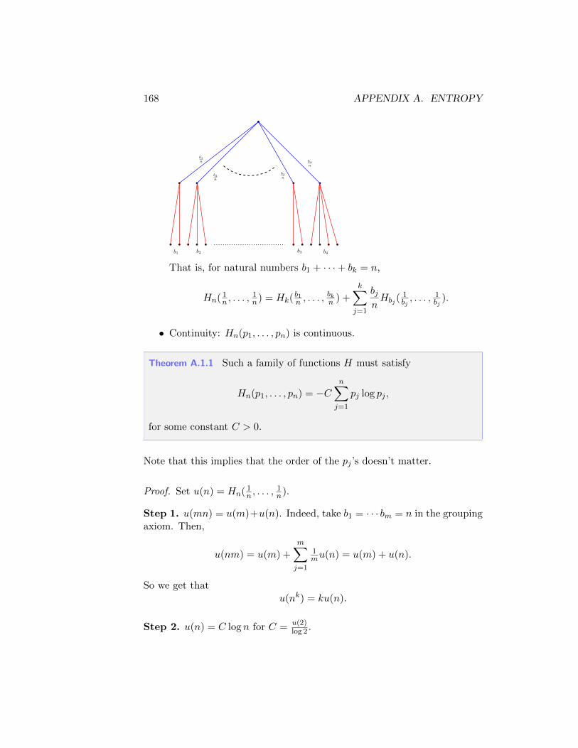
168 APPENDIX A. ENTROPY

b1 b2 b3 b4

b1n

b2n

b3n

b4n

That is, for natural numbers b1 + · · ·+ bk = n,

Hn( 1n , . . . ,

1n) = Hk(

b1n , . . . ,

bkn ) +

k∑j=1

bjnHbj (

1bj, . . . , 1

bj).

• Continuity: Hn(p1, . . . , pn) is continuous.

Theorem A.1.1 Such a family of functions H must satisfy

Hn(p1, . . . , pn) = −Cn∑j=1

pj log pj ,

for some constant C > 0.

Note that this implies that the order of the pj ’s doesn’t matter.

Proof. Set u(n) = Hn( 1n , . . . ,

1n).

Step 1. u(mn) = u(m)+u(n). Indeed, take b1 = · · · bm = n in the groupingaxiom. Then,

u(nm) = u(m) +

m∑j=1

1mu(n) = u(m) + u(n).

So we get thatu(nk) = ku(n).

Step 2. u(n) = C log n for C = u(2)log 2 .

A.1. SHANNON ENTROPY AXIOMS 169

Proof. If n = 1 then grouping implies that

u(n) = u(n) +

n∑j=1

1nH1(1),

so u(1) = H1(1) = 0. So we can assume n > 1.

Let a > 0 be some integer, and let k ∈ N be such that nk ≤ 2a < nk+1.That is, k ≤ a log 2

logn < k + 1 (k = ba log 2logn c).

Here we use that u is strictly increasing: we get

ku(n) = u(nk) ≤ u(2a) = au(2) < u(nk+1) = (k + 1)u(n).

So we have that for any a > 0,

k

a≤ log 2

log n<k + 1

aand

k

a≤ u(2)

u(n)<k + 1

a.

Thus, ∣∣∣∣u(2)

u(n)− log 2

log n

∣∣∣∣ ≤ 1

a.

Taking a→∞ gives the claim. ut

Step 3. Let us prove the theorem for pj ∈ Q. If pj =ajbj∈ Q the define

Πj =∏i 6=j bi and Π =

∏nj=1 bj . So pj =

ajΠjΠ and

∑j ajΠj = Π. Thus, by

grouping,

u(Π) = Hn(a1Π1Π , . . . , anΠn

Π ) +

n∑j=1

ajΠjΠ u(ajΠj).

Rearranging, we have

Hn(p1, . . . , pn) = C log Π− Cn∑j=1

pj log(ajΠj) = −Cn∑j=1

pj log(ajΠj

Π

).

This is the theorem for rational values.

Step 4. The theorem follows for all values by continuity. ut


A.2 A different perspective on entropy

Suppose that we are scientists, we wish to predict the following state of somephysical system. Of course, this is done using previous observations. Sup-pose that the distribution of the next state of the system is distributed overn possible states, say 1, 2, . . . , n. Assume that the (unknown) probabilityfor the system to be in state j is qj . Some scientist provides a prediction forthe distribution: p(1), . . . , p(n). We want to “score” the possible prediction,or rather penalize the prediction based on “how far off” it is from the actualdistribution q1, . . . , qn.

If B(p) is the penalization for predicting a probability p ∈ [0, 1], then theexpected penalization for a prediction p(1), . . . , p(n) is

n∑j=1

qjB(pj).

How would this penalization work?

First, it should be continuous in changing the parameters.

Second, one can predict the distribution after two time steps. So this wouldbe a prediction of a distribution on (i, j) : 1 ≤ i, j ≤ n, denote it byp(i, j). Now, of course scientists all know logic and mathematics, so theirprediction for two time steps ahead is consistent with their prediction forone time step ahead. Specifically, for all i, j we have p(i, j) = p(i|j)p(j).

Also, the penalization for predicting two time steps ahead should be thesame as that for predicting one time step and then predicting the secondstep based on that. That is, B(p(i, j)) = B(p(j)) +B(p(i|j)).

Together with the above p(i, j) = p(i|j)p(j) this becomes: B(xy) = B(x) +B(y) for all x, y ∈ [0, 1].

It is a simple exercise to prove that B(x) = logm x (where the base of thelogarithm is a choice).

Thus, the expected penalization is

H(p(1), . . . , p(n)) = −n∑j=1

qj logm p(j).

A.2. A DIFFERENT PERSPECTIVE ON ENTROPY 171

(Negative sign is to show that this is a penalization.)

Proposition A.2.1 Let pj , qj ∈ (0, 1] be such that∑n

j=1 pj =∑n

j=1 bj = 1.Then, for any m > 1,

−n∑j=1

pj logm pj ≤ −n∑j=1

pj logm qj .

So pj = qj minimizes the expected penalization.

Proof. Note that logm(x) has second derivative − 1x2 logm

< 0 on (0,∞). Soby Jensen’s inequality,

n∑j=1

pj logmqjpj≤ logm

n∑j=1

pjqjpj

= 0.

ut


Appendix B

Hilbert spaces

B.1 Completion

We proceed with a special construction of Hilbert spaces. We are actuallyconstructing an ultraproduct, for more on these see e.g. [?].

Suppose that V is a vector space with inner product 〈·, ·〉V (not necessarilya Hilbert space). Suppose that G acts on V by unitary linear operators;that is, 〈xv, xu〉V = 〈v, u〉V for all v, u ∈ V and x ∈ G.

We define H the completion of V as follows: V∗ be the collection of allCauchy sequences from V . For two sequences α, β ∈ V∗, let d(α, β) =limn ||αn − βn||V . (Here the norm is the induced norm in V .)

Exercise B.1 Show that the limit d(α, β) = limn ||αn−βn||V always existsfor α, β ∈ V∗.

Exercise B.2 Show that α ∼ β ⇐⇒ d(α, β) = 0 defines and equivalencerelation.

Show that if V∗/V0 denotes the set of equivalence classes under this rela-tion, then

[α] + [β] := [α+ β] and λ · [α] := [λ · α]

defines a well defined vector space structure on V∗/V0.

173

174 APPENDIX B. HILBERT SPACES

Show that〈[α], [β]〉 := 〈α, β〉 := lim sup

n〈αn, βn〉V

defines a well defined inner product on V∗/V0.

Show that V∗/V0 is complete (i.e. any Cauchy sequence has a limit). De-duce that V∗/V0 is a Hilbert space.

V∗/V0 is known as the completion of V .

Exercise B.3 Show that the map ϕ(v) := [(v, v, . . .)] ∈ V∗/V0 for v ∈ Vdefines an inner product preserving injective linear map of V into V∗/V0.

Show that ϕ(V ) is dense in V∗/V0.

Exercise B.4 Show that x[α] := [xα] defines a well defined action of G onV∗/V0 by linear operators. (Here xα = (xα0, xα1, . . .).)

Show that 〈x[α], x[β]〉 = 〈[α], [β]〉; that is, the action is unitary.

B.2 Ultraproduct

Let (Hn)n≥0 be a sequence of Hilbert spaces. Suppose that G acts on eachHn by unitary operators. Consider the following construction. Let H =∏nHn (Cartesian product as a set). For any α ∈ H set

||α|| = lim supn→∞

||αn||Hn .

Let H∗ := α ∈ H : ||α|| < ∞, and let H0 := α ∈ H : ||α|| = 0.Note that H0 ≤ H∗ ≤ H are vector spaces under pointwise addition andmultiplication by scalars.

Exercise B.5 Show that α ∼ β ⇐⇒ α− β ∈ H0 defines and equivalencerelation.

Show that if H∗/H0 denotes the set of equivalence classes under this re-lation, then the norm structure on H∗ induces a well defined norm onH∗/H0 by setting ||[α]|| := ||α||.

B.2. ULTRAPRODUCT 175

Show that〈[α], [β]〉 := 〈α, β〉 := lim sup

n〈αn, βn〉Hn

defines a well defined inner product on H∗/H0, whose corresponding normis the same as the above norm.

Exercise B.6 Define an action of G on H∗ by xα = (xα0, xα1, . . .).

Show that if α ∼ β then xα ∼ xβ. (Recall thatG acts by unitary operatorson Hn for each n.)

Show that the action x[α] := [xα] defines a well defined action of G onH∗/H0 by unitary operators.

Finally, we let H be the completion of H∗/H0 and from the above we obtainthat G acts on H by unitary operators. We call H the limit of (Hn)n, anddenote H = limHn.

Exercise B.7 Show that for α ∈ H∗ we have ||[α]||H = lim supn→∞ ||αn||Hn .

All the above culminates in the following construction:

Theorem B.2.1 Let (Hn)n be a sequence of Hilbert spaces. Let G be agroup acting on each Hn by unitary operators. Let

H∗ =

α ∈

∏n

Hn : lim supn||αn||Hn <∞

.

There exists a Hilbert space H and a linear map ϕ : H∗ → H such that〈ϕ(α), ϕ(β)〉 = lim supn 〈αn, βn〉Hn , and such that G acts on H by unitaryoperators, with xϕ(α) = ϕ(xα) for all x ∈ G.

B.2.1 Compact topologies

The natural topology on a Hilbert space is the one induced by the metricgiven by the norm. However, the unit ball is not necessarily compact in thistopology. In fact:


Exercise B.8 Let H be a Hilbert space. Show that the unit ball u ∈ H :||u|| ≤ 1 is compact if and only if dimH <∞.

Solution to ex:8. :(If dimH <∞ then H is isomorphic to Cn for some n so the unit ball is compact. If dimH =∞then let (un)n be an orthonormal sequence. So ||un|| = 1 for all n, and specifically thesequence is in the unit ball, however, for any m 6= n,

||un − um||2 = ||un||2 + ||um||2 = 2,

by Paythagoras, so the sequence does not have a converging subsequence. :) X

Consider a different topology on H. We say that (un)n converges to u weakly(or, in the weak topology), if for any v ∈ H we have 〈un, v〉 → 〈u, v〉.

Exercise B.9 Show that if (un)n converges to u weakly then ||u|| ≤lim infn→∞ ||un||.

Solution to ex:9. :(For any subsequence (unk )k we have

||u||2 = 〈u, u〉 = limk→∞

〈unk , u〉 ≤ lim supk→∞

||unk || · ||u||.

Taking the subsequence fo which lim supk→∞ ||unk || = lim infn→∞ ||un|| completes the proof.:) X

Exercise B.10 Let (qk)k be an orthonormal basis for H.

Show that if (un)n is a sequence in the unit ball, then (un)n convergesweakly to u if and only if for any k we have 〈un − u, qk〉 → 0.

Solution to ex:10. :(Let v ∈ H. Fix ε > 0. Let M be large enough so that ||v − vM || < ε, where vM =∑k≤M 〈v, qk〉 qk. Since vM is a finite linear combination of basis elements, 〈un − u, vM 〉 → 0.

Thus,

| 〈un − u, v〉 | ≤ | 〈un − u, vM 〉 |+ | 〈un − u, v − vM 〉 | ≤ | 〈un − u, vM 〉 |+ supn||un − u|| · ε.

Taking n→∞ and then ε→ 0 completes the proof, utilizing the fact that ||un − u|| ≤ 2. :)X

B.2. ULTRAPRODUCT 177

Exercise B.11 Let (qk)k be an orthonormal basis in H. Show that

ρ(u, v) =∑k

2−k · | 〈u− v, qk〉 |1 + | 〈u− v, qk〉 |

is a metric on H.

Show that ρ induces the weak topology on the unit ball.

Show that ρ(u, v) ≤ 2||u− v||.


ρ(u, v) = ρ(v, u) and ρ(u, v) = 0 iff u = v. Also, as ξ 7→ ξ1+ξ

is an increasing function, we

have that

ρ(u, v) =∑n

2−n ·| 〈u− v, qn〉 |

1 + | 〈u− v, qn〉 |≤∑n

2−n ·| 〈u− w, qn〉 |+ | 〈w − v, qn〉 |

1 + | 〈u− w, qn〉 |+ | 〈w − v, qn〉 |

≤∑n

2−n ·| 〈u− w, qn〉 |

1 + | 〈u− w, qn〉 |+∑n

2−n ·| 〈w − v, qn〉 |

1 + | 〈w − v, qn〉 |= ρ(u,w) + ρ(w, v).

Also, if (un)n converges weakly to u then 〈un − u, qk〉 → 0 for any qk, and thus, it is simple

to see that ρ(un, u)→ 0 (because∑n 2−n <∞ and ξ

1+ξ≤ ξ).

Finally, if ρ(un, u)→ 0 then for any fixed k we have

| 〈un − u, qk〉 |1 + | 〈un − u, qk〉 |

≤ 2k · ρ(un, u)→ 0.

Thus, 〈un − u, qk〉 → 0 for all k. So if (un)n are all in the unit ball then (un)n convergesweakly to u.

Finally, since ξ1+ξ

≤ ξ and since | 〈u− v, qk〉 | ≤ ||u − v|| we have ρ ≤∑k 2−k · ||u − v|| =

2 · ||u− v||. :) X

Theorem B.2.2 Let H be a separable Hilbert space. The unit ball u ∈H : ||u|| ≤ 1 is compact in the weak topology.

Proof. Since the weak topology on the unit ball is metrizable, it suffices toprove that any sequence (un)n with ||un|| ≤ 1 for all n, has a convergingsubsequence in the weak topology.

Let (qk)k be some orthonormal basis.


Let (un)n be any sequence in the unit ball. Fix k. The sequence 〈un, bk〉 isbounded, so admits a converging subsequence. Thus, there is a subsequence(unk,j )j so that

⟨unk,j , bk

⟩→ λk as j → ∞. In fact, we may choose (nk,j)j

as a subsequence of (nk−1,j)j .

Consider the diagonal subsequence vj := unj,j . By construction, for any kwe have that

limj→∞

〈vj , bk〉 = limj→∞

〈uk,j , bk〉 = λk.

By Fatou’s Lemma,∑k

|λk|2 ≤ lim infj→∞

∑k

| 〈vj , bk〉 |2 = lim infj→∞

||vj ||2 ≤ 1.

Thus, u :=∑

k λkbk is a well defined vector in H, and ||u||2 =∑

k |λk|2 ≤ 1so u is in the unit ball.

Note that for any k we have

limj→∞

〈vj − u, bk〉 = 0

which implies that the subsequence (vj)j converges weakly to u. ut


Ariel Yadin - BGU Mathyadina/HFs_notes.pdf · Harmonic functions on groups DRAFT - updated June 19,...

Documents

Transcript of Ariel Yadin - BGU Mathyadina/HFs_notes.pdf · Harmonic functions on groups DRAFT - updated June 19,...