Are Restaurants Really Supersizing America?are.berkeley.edu/~mlanderson/pdf/Anderson and Matsa...
37
152 American Economic Journal: Applied Economics 3 (January 2011): 152–188 http://www.aeaweb.org/articles.php?doi=10.1257/app.3.1.152 “There’s nobody at McDonald’s shoving fries in your mouth.” —Bonnie Modugno, McDonald’s Chief Nutritionist 1 O besity rates in the United States have been growing rapidly in recent years. Whereas 15 percent of Americans were obese in 1980 (defined as having a body mass index of at least 30), 34 percent were obese in 2004 (Center for Disease Control 2007). The time series of obesity rates in the United States, plotted in Figure 1 (solid line), reveals that the rate of increase over the past quarter-century has been substan- tially greater than during the preceding two decades. Medical research has linked obe- sity to diabetes, heart disease, stroke, and certain cancers. Treating these diseases is expensive. Health care spending attributed to obesity reached $78.5 billion in 1998 and continues to grow (Eric A. Finkelstein, Ian C. Fiebelkorn, and Guijing Wang 2003). Although obesity is a serious and growing problem, its causes are not well understood. 1 Kim Severson, “The Obesity Crisis,” San Francisco Chronicle, March 7, 2004. * Anderson: Department of Agricultural and Resource Economics, University of California, Berkeley, 207 Giannini Hall, MC 3310, Berkeley, CA 94720-3310 (e-mail: [email protected]); Matsa: Kellogg School of Management, Northwestern University, 2001 Sheridan Road, Evanston, IL 60208 (e-mail: dmatsa@ kellogg.northwestern.edu). We thank Patricia Anderson, Joshua Angrist, David Card, Carlos Dobkin, Michael Greenstone, Alex Mas, Amalia Miller, Enrico Moretti, Kathryn Shaw, May Wang, and seminar participants at Columbia University, Georgetown University, IUPUI, Northwestern University, Stanford University, Tel Aviv University, UC Berkeley, the 2009 AEA Annual Meeting, and the NBER Summer Institute for helpful comments. Ellen Kersten, David Reynoso, Tammie Vu, and Kristie Wood provided excellent research assistance. We appre- ciate the cooperation of the Departments of Health of Arkansas, Colorado, Iowa, Kansas, Maine, Missouri, North Dakota, Nebraska, Oklahoma, Utah, and Vermont in providing the confidential data used in this study. Their cooperation does not imply endorsement of the conclusions of this paper. † To comment on this article in the online discussion forum, or to view additional materials, visit the article page at http://www.aeaweb.org/articles.php?doi=10.1257/app.3.1.152. Are Restaurants Really Supersizing America? † By Michael L. Anderson and David A. Matsa* While many researchers and policymakers infer from correlations between eating out and body weight that restaurants are a leading cause of obesity, a basic identification problem challenges these con- clusions. We exploit the placement of Interstate Highways in rural areas to obtain exogenous variation in the effective price of restau- rants and examine the impact on body mass. We find no causal link between restaurant consumption and obesity. Analysis of food-intake micro-data suggests that consumers offset calories from restaurant meals by eating less at other times. We conclude that regulation tar- geting restaurants is unlikely to reduce obesity but could decrease consumer welfare. (JEL I12, I18, L51, L66)
Transcript of Are Restaurants Really Supersizing America?are.berkeley.edu/~mlanderson/pdf/Anderson and Matsa...

152
American Economic Journal: Applied Economics 3 (January 2011): 152–188http://www.aeaweb.org/articles.php?doi=10.1257/app.3.1.152
“There’s nobody at McDonald’s shoving fries in your mouth.”—Bonnie Modugno, McDonald’s Chief Nutritionist1
Obesity rates in the United States have been growing rapidly in recent years. Whereas 15 percent of Americans were obese in 1980 (defined as having a body
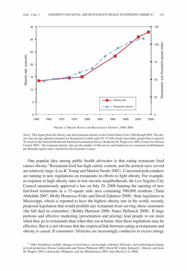
mass index of at least 30), 34 percent were obese in 2004 (Center for Disease Control 2007). The time series of obesity rates in the United States, plotted in Figure 1 (solid line), reveals that the rate of increase over the past quarter-century has been substan-tially greater than during the preceding two decades. Medical research has linked obe-sity to diabetes, heart disease, stroke, and certain cancers. Treating these diseases is expensive. Health care spending attributed to obesity reached $78.5 billion in 1998 and continues to grow (Eric A. Finkelstein, Ian C. Fiebelkorn, and Guijing Wang 2003). Although obesity is a serious and growing problem, its causes are not well understood.
1 Kim Severson, “The Obesity Crisis,” San Francisco Chronicle, March 7, 2004.
* Anderson: Department of Agricultural and Resource Economics, University of California, Berkeley, 207 Giannini Hall, MC 3310, Berkeley, CA 94720-3310 (e-mail: [email protected]); Matsa: Kellogg School of Management, Northwestern University, 2001 Sheridan Road, Evanston, IL 60208 (e-mail: [email protected]). We thank Patricia Anderson, Joshua Angrist, David Card, Carlos Dobkin, Michael Greenstone, Alex Mas, Amalia Miller, Enrico Moretti, Kathryn Shaw, May Wang, and seminar participants at Columbia University, Georgetown University, IUPUI, Northwestern University, Stanford University, Tel Aviv University, UC Berkeley, the 2009 AEA Annual Meeting, and the NBER Summer Institute for helpful comments. Ellen Kersten, David Reynoso, Tammie Vu, and Kristie Wood provided excellent research assistance. We appre-ciate the cooperation of the Departments of Health of Arkansas, Colorado, Iowa, Kansas, Maine, Missouri, North Dakota, Nebraska, Oklahoma, Utah, and Vermont in providing the confidential data used in this study. Their cooperation does not imply endorsement of the conclusions of this paper.
† To comment on this article in the online discussion forum, or to view additional materials, visit the article page at http://www.aeaweb.org/articles.php?doi=10.1257/app.3.1.152.
Are Restaurants Really Supersizing America?†
By Michael L. Anderson and David A. Matsa*
While many researchers and policymakers infer from correlations between eating out and body weight that restaurants are a leading cause of obesity, a basic identification problem challenges these con-clusions. We exploit the placement of Interstate Highways in rural areas to obtain exogenous variation in the effective price of restau-rants and examine the impact on body mass. We find no causal link between restaurant consumption and obesity. Analysis of food-intake micro-data suggests that consumers offset calories from restaurant meals by eating less at other times. We conclude that regulation tar-geting restaurants is unlikely to reduce obesity but could decrease consumer welfare. (JEL I12, I18, L51, L66)
ContentsAre Restaurants Really Supersizing America?† 152
I. Theoretical Framework 156II. Data and Descriptive Statistics 159III. Restaurant Proximity and Body Mass 161A. First-Stage Relation 162B. Reduced-Form Relation 165C. Instrumental Variables Results 168IV. Analysis of Alternative Interpretations 171A. Does Highway Proximity Increase Restaurant Consumption? 171B. Can Residential Sorting across Towns Explain the Results? 176V. Why Don’t Restaurants Affect Obesity? 180VI. Conclusion 184References 186
VoL. 3 No. 1 153ANdErSoN ANd MAtSA: ArE rEStAurANtS rEALLy SupErSIzINg AMErICA?
One popular idea among public health advocates is that eating restaurant food causes obesity.2 Restaurant food has high caloric content, and the portion sizes served are relatively large (Lisa R. Young and Marion Nestle 2002). Concerned policymakers are turning to new regulations on restaurants in efforts to fight obesity. For example, in response to high obesity rates in low-income neighborhoods, the Los Angeles City Council unanimously approved a law on July 29, 2008 banning the opening of new fast-food restaurants in a 32-square mile area containing 500,000 residents (Tami Abdollah 2007; Molly Hennessy-Fiske and David Zahniser 2008). State legislators in Mississippi, which is reported to have the highest obesity rate in the world, recently proposed legislation that would prohibit any restaurant from serving obese customers (the bill died in committee) (Bobby Harrison 2008; Nanci Hellmich 2008). If large portions and effective marketing (presentation and pricing) lead people to eat more when they go to restaurants than when they eat at home, then these regulations may be effective. But it is not obvious that the empirical link between eating at restaurants and obesity is causal. If consumers’ lifestyles are increasingly conducive to excess energy
2 Other hypotheses include changes in food prices, increasingly sedentary lifestyles, and technological change in food production (Darius Lakdawalla and Tomas Philipson 2002; David M. Cutler, Edward L. Glaeser, and Jesse M. Shapiro 2003; Lakdawalla, Philipson, and Jay Bhattacharya 2005; Sara Bleich et al. 2008).
12535
75
100
20
25
30
25
50
5
10
15
Res
taur
ants
(p
er t
hous
and
sq
uare
mile
s)
Ob
esity
rate
(p
erce
nt)
Obesity rate
00
1960 1965 1970 1975 1980 1985 1990 1995 2000 2005
Restaurant density
Figure 1. Obesity Rates and Restaurant Density, 1960–2004
Notes: This figure plots the obesity rate and restaurant density in the United States from 1960 through 2004. The obe-sity rates are age-adjusted estimates for the percent of adults aged 20–74 with a body mass index greater than or equal to 30, based on the National Health and Nutrition Examination Survey (Katherine M. Flegal et al. 2002; Centers for Disease Control 2007). The restaurant density rates are the number of full-service and limited-service restaurant establishments per thousand square miles, reported by the Economic Census.
154 AMErICAN ECoNoMIC JourNAL: AppLIEd ECoNoMICS JANuAry 2011
intake and positive energy balance, the increasing prevalence of restaurants may sim-ply reflect a greater demand for calories.
The case against restaurants centers on well-known correlations showing that the frequency of eating out is positively associated with greater fat, sodium, and total energy intake, as well as with greater body fat. These correlations have been estab-lished using a broad range of datasets and study populations (for examples, see Linda H. Eck Clemens, Deborah L. Slawson, and Robert C. Klesges 1999; M. A. McCrory et al. 1999; J. K. Binkley, J. Eales, and M. Jekanowski 2000; S. A. French, L. Harnack, and R. W. Jeffery 2000; Ashima K. Kant and Barry I. Graubard 2004; J. Maddock 2004; Susan H. Babey et al. 2008). Furthermore, the number of restaurants and the prevalence of obesity have been rising for a number of decades. In addition to the obesity rate, Figure 1 shows the growth of restaurant density in the United States over the past half-century (dashed line). The close correspondence between these series has led some researchers to propose that there is a connection between these trends. Shin Yi Chou, Michael Grossman, and Henry Saffer (2004) examine time-series cor-relations in micro data and infer that the growth in restaurant density accounts for as much as 65 percent of the rise in the percentage of Americans who are obese.3 Despite some evidence that restaurant access does not affect obesity (D. Simmons et al. 2005; Robert W. Jeffery et al. 2006), there appears to be broad consensus among the health policy community that greater availability of restaurants increases body weight (US Department of Health and Human Services 2001; Michelle M. Mello, David M. Studdert, and Troyen A. Brennan 2006; Gary Becker 2007).
But simple correlations between restaurant visits and overeating may conflate the impact of changes in supply and demand. People choose where and how much to eat, leaving restaurant consumption correlated with other dietary practices asso-ciated with weight gain (P. K. Newby et al. 2003; Sahasporn Paeratakul et al. 2003). A key question is whether the growth in eating out is contributing to the obesity epidemic, or whether these changes merely reflect consumer preferences. The interesting causal parameter is how much more an obese person consumes in total because he or she ate at a restaurant. To the extent that changes in preferences are leading consumers to eat out more, regulating restaurants may only lead consum-ers to shift consumption to other sources rather than to reduce total caloric intake.
We present a simple neoclassical model of an optimizing consumer that shows that a rational agent who consumes excess calories at a restaurant will cut back on other caloric intake. An implication of this framework is that eating at restaurants may have little or no causal impact on obesity. The model suggests that consumers’ preference for high caloric intake may explain the observed correlations between restaurant eating and obesity.
To assess the nature of the connection between restaurants and obesity, we exploit variation in the effective price of restaurants (due to the different costs to consumers of traveling to a restaurant) and examine the impact on consumers’ body mass. In rural areas, Interstate Highways provide a variation in the supply of restaurants that is
3 Chou, Grossman, and Saffer (2004, 577) note that their results are generated by “within-state variation over time and by national variation over time.” They explain that they omit national time trends from their regressions to avoid multicolinearity.
VoL. 3 No. 1 155ANdErSoN ANd MAtSA: ArE rEStAurANtS rEALLy SupErSIzINg AMErICA?
arguably uncorrelated with consumer demand. To serve the large market of highway travelers passing through, a disproportionate number of restaurants locate immedi-ately adjacent to these highways. For residents of these communities, we find that the highway boosts the supply of restaurants (and reduces the travel cost associated with visiting a restaurant) in a manner that is plausibly uncorrelated with demand or gen-eral health practices. Using original survey data based on a smaller sample, we show that differences in travel costs generate large differences in restaurant consumption. To uncover the causal effect of restaurants on obesity, we compare the prevalence of obesity in communities located immediately adjacent to Interstate Highways with the prevalence of obesity in communities located slightly farther away. Although average travel distances to restaurants differ in rural and urban areas, the financial interpreta-tion of these distance costs is generalizable to both settings.
The estimates suggest that restaurants—both fast food and full service—have little effect on adult obesity. The distributions of BMI in highway and nonhighway areas are virtually identical, and point estimates of the causal effect of restaurants on the prevalence of obesity are close to zero and precise enough to rule out any meaning-ful effects. These results indicate that policies focused on reducing caloric intake at restaurants are unlikely to substantially reduce obesity, at least for adults. Two recent papers developed in parallel with this research, Brennan Davis and Christopher Carpenter (2009) and Janet Currie at al. (2010), come to qualitatively similar con-clusions regarding children. These papers examine the reduced-form relationship between fast-food proximity and childhood obesity in several states using school-level data. They find that schools located near fast-food restaurants have higher child-hood obesity rates, but that the magnitude of this relationship is small. Currie et al. (2010) also estimate the relationship between fast-food restaurant proximity and weight gain among pregnant women, and find a small but statistically significant relationship.4 Although our three studies focus on different populations (adults versus children) and exploit different types of identification (we instrument for restaurant placement whereas the other studies use observed restaurant placement), all three papers conclude that fast-food availability is not a primary determinant of obesity.
Given that a typical restaurant meal contains more calories than a home-cooked meal, it may seem surprising that lowering restaurant prices does not increase obesity. Our neoclassical model of a rational consumer points to two characteristics of con-sumer preferences that could explain this phenomenon: heterogeneity in desired caloric intake and satiation. Heterogeneity in desired caloric intake could generate a positive correlation between caloric intake and restaurant meals if people who eat large meals also prefer to eat at restaurants. Satiation could induce individuals to offset calories eaten at restaurants by reducing caloric consumption at other times during the day. In either case, a positive correlation between caloric intake and restaurant meals does not necessarily imply that restaurants have a causal effect on total calories consumed.
4 Davis and Carpenter (2009) find that a one mile decrease in distance to the nearest fast-food restaurant is associated with an average increase of 0.03 BMI points (less than 0.01 standard deviations). Under any nontrivial value for travel costs, this result implies that changes in the effective price of fast food have a negligible impact on average BMI. Currie et al. (2010) conclude from their estimates that changes in fast-food restaurant availability could explain no more than 0.5 percent of the increase in obesity over the last 30 years among ninth graders and 2.7 percent of the increase in weight over the last 10 years among women.
156 AMErICAN ECoNoMIC JourNAL: AppLIEd ECoNoMICS JANuAry 2011
To test for these effects, we examine food intake data collected by the US Department of Agriculture (USDA). These micro data contain information on all food items consumed by a large panel of individuals. We find evidence of both heterogeneity and satiation. First, there is selection bias in who eats at restaurants. People who eat at restaurants also consume more calories than other consumers when they eat at home. Second, when including individual fixed effects, we find that people who eat large portions in restaurants tend to reduce their calorie consump-tion at other times during the day. After accounting for these factors, we find that although the average restaurant meal contains approximately 250 calories more than the average meal eaten at home, the existence of restaurants increases BMI by only 0.2 BMI points for the typical obese consumer.
These food intake results have broad implications for obesity policy and general health and safety regulation. Economic theory implies that regulating specific inputs in the health production function may not improve outcomes if consumers can compensate in other ways. This proposition is supported by economic studies in a variety of empirical settings. For example, Sam Peltzman (1975) contends that man-dating automobile safety devices does not reduce traffic fatalities because motor-ists respond by driving less carefully. More recently, Jerome Adda and Francesca Cornaglia (2006) have argued that smokers react to cigarette taxes by smoking fewer cigarettes more intensively.
In the case of obesity, consumers have access to multiple sources of cheap calo-ries. Restricting a single source—such as restaurants—is therefore unlikely to affect obesity, as our findings confirm. This mechanism may underlie the apparent failure of so many interventions targeted at reducing obesity (Gina Kolata 2006). Despite their ineffectiveness, however, such policies have the potential to generate consider-able deadweight loss. Our results suggest that obesity reductions are unlikely in the absence of more comprehensive policies.
I. Theoretical Framework
The fundamental economic forces underlying the obesity epidemic are not well understood. Although obesity may be the consequence of lifetime-utility-maximizing consumers making informed decisions about eating and exercising, self-control issues likely also lead some consumers to overeat (Cutler, Glaeser, and Shapiro 2003). While food brings immediate gratification, the health costs of over-consumption occur in the future. If consumer preferences are time inconsis-tent, then regulation aimed at decreasing obesity may benefit at-risk individuals. The costs of treating obesity are also unlikely to be fully internalized by consum-ers.5 The goal of this paper is not to evaluate how time inconsistency or externali-ties affect the optimality of decisions regarding caloric intake. Rather, we assume that the prevalence of obesity is socially suboptimal and take reducing obesity rates to be a public policy objective. In this context, we aim to evaluate whether
5 Finkelstein, Fiebelkorn, and Wang (2003) estimate that Medicare and Medicaid alone spent $37.6 billion covering obesity-related illnesses in 1998 ($55.6 billion in 2007 dollars, inflated with CPI Medical Care Services index).
VoL. 3 No. 1 157ANdErSoN ANd MAtSA: ArE rEStAurANtS rEALLy SupErSIzINg AMErICA?
regulations focused on raising the effective price of restaurants are likely to suc-ceed in reducing obesity.
Recognizing that consumers are optimizing agents reveals other characteristics of consumer preferences that are likely to undermine the efficacy of these regula-tions. To illustrate these challenges for public policy, we present a simple model of an optimizing consumer’s decision about how much to eat. For simplicity, we abstract away from issues related to time inconsistency and focus on the impact of neoclassical characteristics of consumer preferences that are present even in a static model. This modeling approach is similar to that used by Thomas D. Jeitschko and Rowena A. Pecchenino (2006), who argue that the socially optimal size of restau-rant meals is larger than the size of the average home-cooked meal—even though the larger portion size leads some consumers to overeat. Our model is also related to the dynamic theory of weight management developed by Lakdawalla and Philipson (2002), which also models food intake by an optimizing consumer. While they use a dynamic model to examine how changes in average food prices, income, and physi-cal activity affect steady-state weight, we use a simpler static model to illustrate how changes in the relative prices of specific foods affect total food consumption. Our conclusions extend to the dynamic weight-management framework.
Consider a rational agent who chooses how many calories to consume during each of two periods—mealtime (c1) and snack-time (c2). Meals can be consumed either at home or at a restaurant. Eating at home costs the agent p1H per calorie consumed as well as a fixed cost f1H, representing the time it takes to prepare the meal. Some days the agent is busier than others, and f1H is a random variable drawn daily from a support of [0, ∞). Alternatively, the agent can eat out during mealtime. Eating at a restaurant costs the agent f1r for a set quantity of food k, including the price of the meal and the time cost of traveling to and from the restaurant. Eating at snack-time costs the agent p2 per calorie.
For simplicity, suppose calories consumed at a restaurant are perfect substitutes for calories consumed at home and that the agent has quasi-linear preferences in caloric consumption and another composite good x (Jeitschko and Pecchenino 2006):6
(1) u = u (c1H + c1r, c2) + x.
Caloric intake at mealtime is a substitute for caloric intake at snack-time in the sense that eating more at mealtime decreases the marginal utility of eating more at snack-time and vice versa, u c 1 c 2 < 0. Suppose that the consumer’s income y is great enough that she consumes a positive amount of the composite good. An optimizing consumer chooses how much to eat to maximize her utility subject to her budget constraint:
(2) y − I (c1H > 0)( f1H + p1H c1H) − I (c1r > 0)( f1r) − p2 c2 − x ≥ 0.
6 Quasi-linear preferences are a plausible assumption for a consumer whose income is sufficiently large and for whom food is only a small part of his total budget.
158 AMErICAN ECoNoMIC JourNAL: AppLIEd ECoNoMICS JANuAry 2011
Following Young and Nestle (2002), assume that restaurant portion sizes are relatively large (i.e., larger than the agent would choose to eat at home, k > c 1H * ). Depending on idiosyncratic circumstances on a particular day (her draw of f1H), the agent will eat the meal either at home or at a restaurant, but not in both places. Let c 1H * and c 2 * (H) denote the chosen levels of caloric consumption at mealtime and snack-time, respectively, when the agent eats the meal at home, and let c 1r * and c 2 * (r) denote the chosen levels of caloric consumption when the agent eats the meal at a restaurant. Three results immediately follow from this framework.
RESULT 1: c 1r * > c 1H * . On days when the agent eats at a restaurant, she eats more at mealtime than on days when she prepares the meal at home. The agent eats more at a restaurant because the marginal cost of additional caloric intake is lower than at home.7 At a restaurant, the fixed pricing scheme leads the agent not to internalize marginal production costs; she eats until she either finishes the portion, c 1r * = k, or is completely satiated, u c 1r * = 0. At home, she stops eating sooner, when marginal utility equals marginal cost, u c 1r * = p1H. The agent “overeats” in restaurants in the sense that she consumes calories for which her marginal utility exceeds the marginal production cost.
RESULT 2: c 2 * (r) < c 2 * (H ). On days when the agent eats at a restaurant, she eats less at snack-time than on days when she eats the meal at home. At snack-time, the agent eats until marginal utility equals marginal cost, u c 2 * = p2. Because calo-ries at mealtime and snack-time are substitutes, u c 1 c 2 < 0, the agent compensates for the larger portions at restaurants by consuming less throughout the rest of the day. Adding together calories consumed at mealtime and snack-time, total caloric intake is not necessarily greater on days when the agent eats at a restaurant. In this framework, decreasing the price of restaurant food, f1r, makes the agent more likely to eat at a restaurant, which increases consumption at that meal, but may or may not increase total caloric intake.
RESULT 3: Total caloric intake depends on u(∙). Even if food prices are constant across the population, total caloric intake varies from person to person, depending on the agent’s preferences. Variation in consumer preferences for caloric intake may lead some individuals to eat more than others—regardless of whether they are eat-ing at a restaurant or at home. If consumers with a preference for high caloric intake patronize restaurants more frequently than others, then the empirical association of eating out and obesity would not reflect a causal relationship.
Whether restaurants actually increase obesity is an empirical question, and OLS estimates of the relationship between eating out and caloric intake are likely to give misleading results. It is possible that access to large portions with low
7 For simplicity, we do not model explicitly the agent’s option to save unconsumed food purchased from the restaurant for other meals or snacks. Implicitly, this sort of transfer between meals is one form of calorie offsetting addressed by Result 2, and it works to undermine a causal effect of restaurant portion size on obesity. Nevertheless, to the extent that physically transferring food between meals is costly (for example, if food quality is reduced or if there is a chance of spoilage), this sort of direct offsetting is unlikely to be complete.
VoL. 3 No. 1 159ANdErSoN ANd MAtSA: ArE rEStAurANtS rEALLy SupErSIzINg AMErICA?
marginal costs at restaurants leads people to overeat. On the other hand, if ratio-nal consumers compensate for large restaurant portions by eating less elsewhere, raising restaurants’ effective prices may have no impact on total caloric intake or obesity. The empirical analysis that follows addresses this important question in two stages. First, in Sections II–IV, we implement an instrumental variables design using Interstate Highways to estimate the reduced form effect of restau-rants on obesity. Then in Section V, we examine USDA food intake data to test whether consumer heterogeneity and offsetting behavior diminish the net effect of restaurants on total caloric intake.
II. Data and Descriptive Statistics
The obesity data used in this study come from a confidential extract of the Behavioral Risk Factor Surveillance System (BRFSS). BRFSS is an ongoing, large-scale telephone survey that interviews hundreds of thousands of individuals each year regarding their health behaviors. In addition to questions about demographic characteristics and health behaviors, BRFSS asks each individual to report his or her weight and height.
Two features of BRFSS are important for our study. First, BRFSS generally oversamples less populous states. Since our analysis focuses on rural areas, this sampling frame works to our advantage. Second, although consolidated BRFSS data are publicly available from the Centers for Disease Control (CDC), CDC does not release geographic identifiers at a finer level than the county. To complete our study, we therefore approached 23 state departments of health and requested confidential BRFSS extracts that include a much finer geographic identifier: telephone area code and exchange (i.e., the first 6 digits of a 10-digit telephone number). Ultimately, 11 states—Arkansas, Colorado, Iowa, Kansas, Maine, Missouri, North Dakota, Nebraska, Oklahoma, Utah, and Vermont—cooperated with our requests. Sample years vary by state and overall cover 1990 through 2005.
Our measures of obesity include body mass index (BMI)—defined as weight in kilograms divided by height in meters squared—and overweight and obese indicators that equal unity if BMI is greater than 25 or 30, respectively. These measures are stan-dard in the obesity literature, and the obese indicator is of particular interest because mortality risk increases as BMI exceeds 30 (Kenneth F. Adams et al. 2006). Data on height and weight in the BRFSS are self-reported. Although some respondents may misreport this information, John H. Cawley (1999) and Majid Ezzati et al. (2006) find the degree of misreporting to be minimal, and there is no reason to suspect that misre-porting would be more or less prevalent in rural towns adjacent to Interstate Highways (our instrument for restaurant proximity) than in other nearby towns.
Restaurant establishment data are from the United States Census ZIP Code Business Patterns. These data include separate counts of full-service (“sit-down”) and limited-service (“fast-food”) restaurants for every ZIP code in the United States.8 We examine the effects of both types of restaurants in this study. Fast-food
8 The distinction between full-service and limited-service restaurants is based on the timing of payment. In full-service restaurants, the customer pays after eating. In limited-service restaurants, the customer pays before eating.
160 AMErICAN ECoNoMIC JourNAL: AppLIEd ECoNoMICS JANuAry 2011
restaurants are usually busiest at lunchtime, and their most popular menu type is hamburgers (43 percent of sales), followed by pizza (13 percent), sandwich/sub (10 percent), chicken (9 percent), and Mexican (8 percent) (US Census Bureau 2005). A majority of these establishments (65 percent of sales) operate under a trade name. US sales at McDonald’s, the largest chain, totaled almost $29 billion in 2007—over three times more than its closest rival (Technomic Information Services 2008). Other fast-food chains with over $5 billion in US sales include Burger King, Subway, Wendy’s, Taco Bell, and KFC. Sit-down restaurants, on the other hand, are usually busiest at dinnertime, rarely operate under a trade name (12 percent of sales), and tend to serve “American” food (47 percent). The largest sit-down chains include Pizza Hut, Applebee’s, Chili’s, and Olive Garden. The average price of a sit-down meal is more than twice that of fast food—$12.30 versus $5.51, excluding tax and tip (US Census Bureau 2005).
Ideally we would have individual-level data on frequency of restaurant consump-tion to document the relationship between restaurant consumption and Interstate proximity. To our knowledge, however, no existing datasets with this information have both the necessary geographical detail and sampling rates to provide a sample of meaningful size in our study areas. Instead, we conduct our own survey on fre-quency of restaurant consumption, described in Section IVA.
Because the restaurant data are identified by ZIP code and the obesity data are identified by telephone exchange, it is impossible to create an exact link between the two datasets. Instead, our analysis relies on two-sample-instrumental-variables tech-niques, which use separate samples to estimate the effect of the instrument on each of the two endogenous variables, obesity and restaurant access. The link between the two datasets thus runs through the instrument—proximity to an Interstate Highway. The results are also robust to two-stage-least-squares estimation on the subsample for which the geographic identifiers line up. (See Online Appendix A for additional details on the construction of the main analytic sample and these robustness checks.)
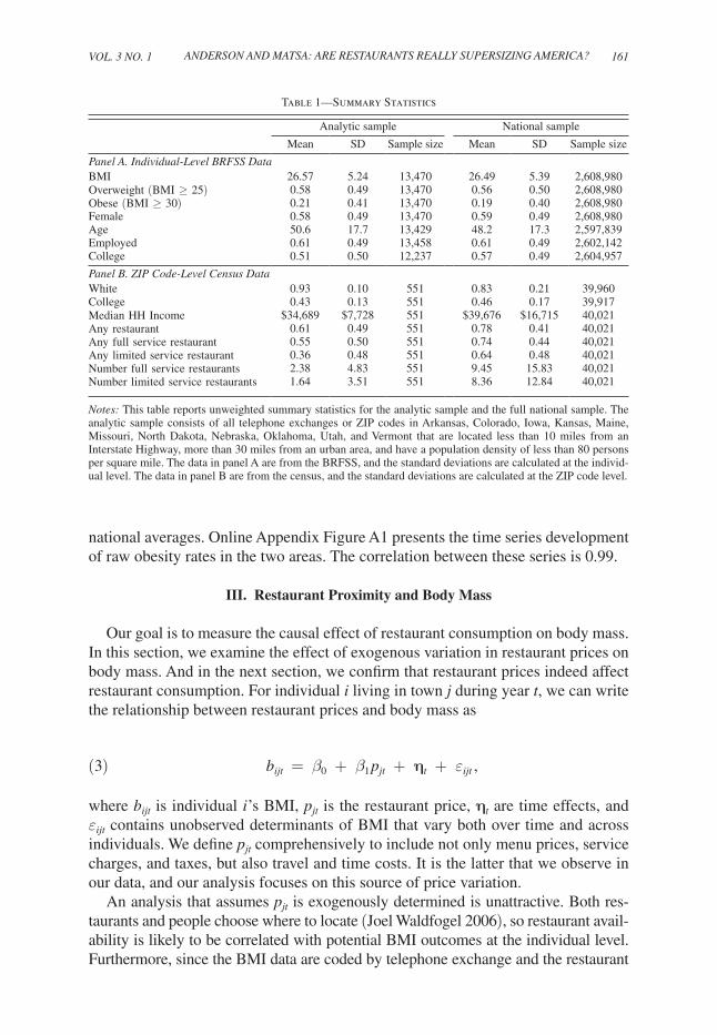
Table 1 presents summary statistics for our datasets. The first two columns present unweighted means and standard deviations for the analytic sample, which consists of all telephone exchanges or ZIP codes in cooperating states located less than 10 miles from an Interstate Highway, more than 30 miles from an urban area, and with a population density of less than 80 persons per square mile. Our analysis focuses on rural areas because the population density in urban areas guarantees that almost everyone has easy access to one or more restaurants. (We also present estimates for alternative samples that have population densities of less than 40 or 160 persons per square mile; the results are qualitatively unchanged.) The last set of columns in Table 1 present the same statistics for the full national sample.
Table 1, panel A, based on BRFSS data, reveals that average BMI, percent over-weight, and percent obese in the analytic sample closely match national averages. The analytic sample is slightly older and somewhat less educated than the national sample. Panel B, based on census data, shows that the rural analytic sample has fewer minorities and a lower average income than the national sample. The analytic sample also has substantially fewer restaurants per ZIP code than the national sam-ple, primarily because the average population per ZIP code is much lower. Trends in obesity rates in geographic areas that contain the analytic sample also closely match
VoL. 3 No. 1 161ANdErSoN ANd MAtSA: ArE rEStAurANtS rEALLy SupErSIzINg AMErICA?
national averages. Online Appendix Figure A1 presents the time series development of raw obesity rates in the two areas. The correlation between these series is 0.99.
III. Restaurant Proximity and Body Mass
Our goal is to measure the causal effect of restaurant consumption on body mass. In this section, we examine the effect of exogenous variation in restaurant prices on body mass. And in the next section, we confirm that restaurant prices indeed affect restaurant consumption. For individual i living in town j during year t, we can write the relationship between restaurant prices and body mass as
(3) bijt = β0 + β1 pjt + ηt + εijt ,
where bijt is individual i ’s BMI, pjt is the restaurant price, ηt are time effects, and εijt contains unobserved determinants of BMI that vary both over time and across individuals. We define pjt comprehensively to include not only menu prices, service charges, and taxes, but also travel and time costs. It is the latter that we observe in our data, and our analysis focuses on this source of price variation.
An analysis that assumes pjt is exogenously determined is unattractive. Both res-taurants and people choose where to locate (Joel Waldfogel 2006), so restaurant avail-ability is likely to be correlated with potential BMI outcomes at the individual level. Furthermore, since the BMI data are coded by telephone exchange and the restaurant
Table 1—Summary Statistics
Analytic sample National sample
Mean SD Sample size Mean SD Sample size
panel A. Individual-Level BrFSS dataBMI 26.57 5.24 13,470 26.49 5.39 2,608,980Overweight (BMI ≥ 25) 0.58 0.49 13,470 0.56 0.50 2,608,980Obese (BMI ≥ 30) 0.21 0.41 13,470 0.19 0.40 2,608,980Female 0.58 0.49 13,470 0.59 0.49 2,608,980Age 50.6 17.7 13,429 48.2 17.3 2,597,839Employed 0.61 0.49 13,458 0.61 0.49 2,602,142College 0.51 0.50 12,237 0.57 0.49 2,604,957
panel B. zIp Code-Level Census dataWhite 0.93 0.10 551 0.83 0.21 39,960College 0.43 0.13 551 0.46 0.17 39,917Median HH Income $34,689 $7,728 551 $39,676 $16,715 40,021Any restaurant 0.61 0.49 551 0.78 0.41 40,021Any full service restaurant 0.55 0.50 551 0.74 0.44 40,021Any limited service restaurant 0.36 0.48 551 0.64 0.48 40,021Number full service restaurants 2.38 4.83 551 9.45 15.83 40,021Number limited service restaurants 1.64 3.51 551 8.36 12.84 40,021
Notes: This table reports unweighted summary statistics for the analytic sample and the full national sample. The analytic sample consists of all telephone exchanges or ZIP codes in Arkansas, Colorado, Iowa, Kansas, Maine, Missouri, North Dakota, Nebraska, Oklahoma, Utah, and Vermont that are located less than 10 miles from an Interstate Highway, more than 30 miles from an urban area, and have a population density of less than 80 persons per square mile. The data in panel A are from the BRFSS, and the standard deviations are calculated at the individ-ual level. The data in panel B are from the census, and the standard deviations are calculated at the ZIP code level.

162 AMErICAN ECoNoMIC JourNAL: AppLIEd ECoNoMICS JANuAry 2011
data are coded by ZIP code, combining bijt and pjt in a single sample is infeasible. (As a robustness check, we show that the results also hold using single-sample estimation for the 60 percent of BRFSS respondents for whom we observe the correct ZIP code with certainty.) We address these issues by finding an instrument zj that satisfies two essential properties. First, it affects restaurant availability, and second, it is uncorre-lated with other determinants of potential BMI outcomes, εijt .
Our instrument, zj, exploits the location of Interstate Highways in rural areas as a source of exogenous variation in restaurant placement. We compare two groups of small towns: those directly adjacent to an Interstate Highway (0–5 miles away) and those slightly farther from an Interstate (5–10 miles away). For convenience, we refer to these two sets of towns as “adjacent” and “nonadjacent,” respectively; example towns are mapped in Online Appendix Figure A2. The Interstate Highways were designed in the 1940s “to connect by routes, direct as practical, the prin-cipal metropolitan areas, cities, and industrial centers” of the United States (US Department of Transportation 2002). As an unintended consequence, the highways lowered transportation costs for rural towns that happened to lie on highway routes running between major cities. We thus use straight-line distance to the highway as an instrument for highway access. We show that this variation is sufficient to gen-erate substantial differences in both restaurant access and consumption. We avoid using distance to the nearest highway exit in constructing the instrument because the placement of exits is likely endogenously determined by town characteristics (nevertheless, our results are robust to either measure).
Previous work has studied the effects of highways on rural county-level eco-nomic outcomes (Amitabh Chandra and Eric Thompson 2000; Guy Michaels 2008). These studies conclude that highways can affect county-level economic outcomes. To avoid this problem, our study uses a much finer level of geographic detail—ZIP codes and telephone exchange areas.9 This geographic detail enables us to limit our sample to ZIP codes and exchanges for which the center lies within 10 miles of an Interstate Highway. (See Online Appendix Figure A2 for a map depicting the level of geographic detail.) We therefore expect—and find—no systematic differences in economic outcomes between the two groups of towns in our sample.
A. First-Stage relation
For a large group of individuals—through travelers on Interstate Highways—adjacent towns represent a more convenient service option than nonadjacent towns that are even slightly farther away. Since these individuals have many choices along their route of travel, their demand is highly elastic with respect to distance from the highway. Proximity to an Interstate thereby increases the supply of restaurants in towns adjacent to Interstates, relative to towns that are not immediately adjacent, for a reason that is independent of local demand (as long as residents do not sort
9 The average US county contains approximately 1,030 square miles, whereas the average US ZIP code contains approximately 80 square miles (US Census Bureau 2002a, 2002b). Telephone exchanges are even smaller than ZIP codes. There are approximately 35,000 ZIP codes and 130,000 telephone exchanges in the United States. However, the differential in geographic area between ZIP codes and exchanges is not as large as it appears because telephone exchanges in urban areas can overlap whereas ZIP codes do not.
VoL. 3 No. 1 163ANdErSoN ANd MAtSA: ArE rEStAurANtS rEALLy SupErSIzINg AMErICA?
to different areas based on the availability of restaurants, an issue that we consider below). In a comparison of the two sets of towns, ZIP codes located 0–5 miles from Interstates are approximately 38 percent (19 percentage points) more likely to have restaurants than ZIP codes located 5–10 miles from Interstates. This is true for both fast-food and full-service restaurants.
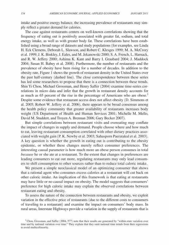
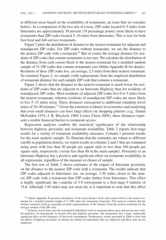
Figure 2 plots the distribution of distance to the nearest restaurant for adjacent and nonadjacent ZIP codes. For ZIP codes without restaurants, we use the distance to the nearest ZIP code with a restaurant.10 But of course the average distance for resi-dents of ZIP codes that contain restaurants is not zero. We calculate the distribution of the distance from each census block to the nearest restaurant for a stratified random sample of 21 ZIP codes that contain restaurants (see Online Appendix B for details). Residents of these ZIP codes live, on average, 2.5 miles from their nearest restaurant. To construct Figure 2, we sample (with replacement) from the empirical distribution of restaurant distance for each sample ZIP code that contains a restaurant.
Figure 2 shows that the distance to the nearest restaurant is much lower for resi-dents of ZIP codes that are adjacent to an Interstate Highway than for residents of nonadjacent ZIP codes. Most residents of adjacent ZIP codes live 0 to 5 miles from the nearest restaurant, whereas residents of nonadjacent ZIP codes are more likely to live 5–15 miles away. These distances correspond to additional roundtrip travel times of 10–40 minutes.11 Given the extensive evidence in economics and marketing that even small distances can have large effects on shopping patterns (e.g., Daniel McFadden 1974; J. R. Blaylock 1989; Lesley Chiou 2009), these distances repre-sent a sizable financial barrier to restaurant access.
Regression analyses confirm the statistical significance of the relationship between highway proximity and restaurant availability. Table 2 reports first-stage results for a variety of restaurant availability measures. Column 1 presents results for the main analytic sample. To illustrate that the estimates are robust to different cutoffs in population density, we report results in columns 2 and 3 that are estimated using areas with less than 40 people per square mile or less than 160 people per square mile, respectively (versus less than 80 in the main sample). Proximity to an Interstate Highway has a positive and significant effect on restaurant availability in all regressions, regardless of the measure or choice of sample.
The first row of Table 2 shows estimates of the impact of Interstate proximity on the distance to the nearest ZIP code with a restaurant. The results indicate that ZIP codes adjacent to Interstates are, on average, 1.50 miles closer to the near-est ZIP code with a restaurant than ZIP codes farther from Interstates. This effect is highly significant; the t-statistic of 3.9 corresponds to a first-stage F-statistic of 15.6. Although 1.50 miles may not seem far, it is important to note that this effect
10 Online Appendix B presents calculations of the exact distance from each census block to the nearest res-taurant for a stratified random sample of 11 ZIP codes not containing restaurants. This analysis confirms that the distance measures used are generally accurate representations of the distance from the nearest restaurant for the average resident of the ZIP code.
11 In theory, travel times may be overstated if individuals work in restaurant-dense areas and eat out near work. Nevertheless, we demonstrate in Section IVA that highway proximity (the instrument) has a large, statistically significant effect on the frequency of fast-food consumption. Furthermore, results presented in Table 4 show that the effects of highway proximity on obesity are similar for individuals who are employed and those who are not employed.

164 AMErICAN ECoNoMIC JourNAL: AppLIEd ECoNoMICS JANuAry 2011
0.15
Nonadjacent
0.1
0.05
Den
sity
0
0 5 10 15 20 25 30
Miles
Nonadjacent
Adjacent
Figure 2. Distribution of Distance to Nearest Restaurant in Towns Adjacent and Nonadjacent to Interstate Highways
Notes: This figure plots the distribution of distance to the nearest restaurant for towns that are adjacent and nonadja-cent to Interstate Highways. For ZIP codes without restaurants, we use distance to the nearest ZIP code with a restaurant. For ZIP codes with restaurants, we sample (with replacement) from the empirical distribution of distance to the near-est restaurant for each census block in a stratified random sample of 21 ZIP codes (see Online Appendix B for details).
Table 2—First-Stage Effect of Interstate Proximity on Restaurant Access
Dependent variable (1) (2) (3)
Miles to nearest ZIP with restaurant −1.50 −1.38 −1.64(0.39) (0.45) (0.36)
Any restaurant 0.175 0.165 0.208(0.042) (0.047) (0.039)
Any full-service restaurant 0.196 0.188 0.228(0.042) (0.046) (0.040)
Any limited-service restaurant 0.154 0.131 0.210(0.040) (0.043) (0.038)
Restaurants per 1,000 people 0.55 0.63 0.56(0.19) (0.21) (0.18)
Travel cost −$2.10 −$1.94 −$2.30(0.55) (0.64) (0.50)
Sample: Population density cutoff (people per square mile) 80 40 160 Number of ZIP codes 551 460 625
Notes: In this table, each coefficient represents a separate regression. The reported coefficients are from regres-sions of the specified dependent variables on an indicator for whether the respondent’s ZIP code is adjacent to an Interstate Highway. All regressions contain state-by-year fixed effects. Robust standard errors are reported in parentheses.

VoL. 3 No. 1 165ANdErSoN ANd MAtSA: ArE rEStAurANtS rEALLy SupErSIzINg AMErICA?
primarily operates through the differential in ZIP codes containing any restaurants. Proximity to an Interstate makes a ZIP code more likely to have a restaurant, reduc-ing the average distance to the nearest ZIP code with a restaurant from 10.2 miles to 2.5 miles. Thus, although the majority of the sample is unaffected, those that are affected have much lower travel costs.
Our instrumental variables results focus on travel distance as the relevant measure of restaurant access because it has a direct economic interpretation. Nevertheless, other estimates, reported in Table 2, show that the relationship between Interstate proximity and restaurant availability is robust across different measures. ZIP codes adjacent to Interstates are 17.5 percentage points more likely to contain at least one restaurant (t = 4.2). This effect holds for both full-service and limited-service (fast-food) restaurants. Although the effect for full-service restaurants is larger in raw percentage point terms (19.6 percentage point increase versus 15.4 percentage point increase), the effect for limited-service restaurants is larger in proportional terms (45.6 percent increase versus 57.9 percent increase). ZIP codes adjacent to Interstates also have a greater density of restaurants, as measured by restaurants per capita.
The effect of interest for public policy is the response in BMI to changes in total restaurant price. We translate the distance measure reported in the first row of Table 2 into a price measure using conservative estimates of vehicle operating costs and travel time valuation. (See Online Appendix C for a description of the meth-odology.) We estimate total travel costs, including both vehicle operating costs and travel time, at 70.1 cents per mile. The last row of Table 2 indicates that the average cost differential in restaurant access for ZIP codes adjacent to Interstates versus ZIP codes farther from Interstates is $2.10 (1.50 miles × 2 directions × 70.1 cents/mile = $2.10). As explained above, this effect operates through the differential in ZIP codes containing any restaurants. Proximity to an Interstate reduces the total restaurant price by an average of $10.80 for areas that would not have a restaurant if not for the highway. This figure corresponds to almost twice the average menu price of a fast-food meal and to 88 percent of the average menu price of a sit-down restaurant meal.
B. reduced-Form relation
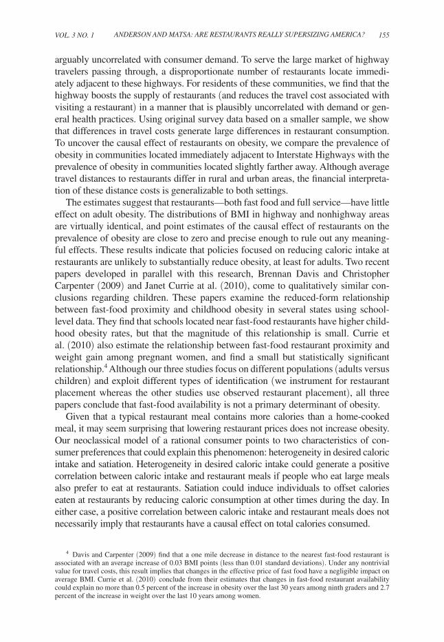
Figure 3 presents the distribution of BMI for towns adjacent to an Interstate and towns farther from an Interstate. The two distributions match up exactly, suggesting that restaurants have no discernable effect on any quantile of the obesity distribution.
Table 3 reports regression coefficients measuring the reduced-form effect of Interstate proximity on body mass. These estimates come from the regression:
(4) bikst = α0 + α1zkst + ϕst + vikst,
where bikst is the BMI, overweight, or obese status of person i in telephone exchange k of state s in year t, zkst is an indicator for proximity to an Interstate (equal to unity if within five miles of an Interstate and zero otherwise), ϕst are state-by-year fixed effects, and vikst is the least squares residual. The first row shows estimates of the

166 AMErICAN ECoNoMIC JourNAL: AppLIEd ECoNoMICS JANuAry 2011
impact of Interstate proximity on an obese indicator (BMI > 30), the second row shows estimates of the impact on an overweight indicator (BMI > 25), and the third row shows estimates of the impact on BMI. Public health practitioners often focus on the first measure because mortality risk does not increase substantially until BMI is above 30. Column 1 reports estimates from the full analytic sample and includes controls for state-by-year fixed effects, but no other covariates. The regressions are precisely estimated. The estimated coefficient from the obese regression indicates that proximity to a highway has no significant effect on the probability of being obese. In fact, the point estimate is negative (−0.1 percentage points). Estimates from the overweight and BMI regressions also show that proximity to highways does not affect body weight. The BMI coefficient is statistically insignificant and implies that Interstate proximity increases BMI by only 0.002 points.12
The reduced-form results are robust to various adjustments to the econometric specification. Column 2 reports results from regressions that contain no state or year fixed effects. The coefficients are close to those reported in column 1 and remain
12 Specifying BMI in logs, rather than levels, also generates a regression coefficient that is close to zero (0.0001) and statistically insignificant.
0.08
0.06
0.02
0.04
0
0 20 40 60 80
BMI
Adjacent
Nonadjacent
Den
sity
Figure 3. Distribution of Body Mass Index in Towns Adjacent and Nonadjacent to Interstate Highways
Note: This figure plots the distribution of body mass index (BMI) for residents of towns that are adjacent and non-adjacent to Interstate Highways.
VoL. 3 No. 1 167ANdErSoN ANd MAtSA: ArE rEStAurANtS rEALLy SupErSIzINg AMErICA?
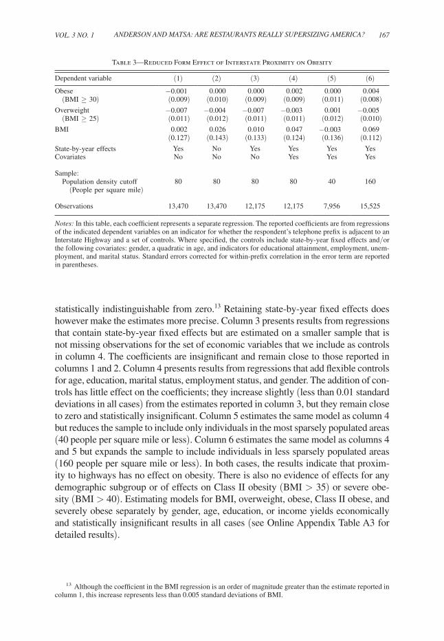
statistically indistinguishable from zero.13 Retaining state-by-year fixed effects does however make the estimates more precise. Column 3 presents results from regressions that contain state-by-year fixed effects but are estimated on a smaller sample that is not missing observations for the set of economic variables that we include as controls in column 4. The coefficients are insignificant and remain close to those reported in columns 1 and 2. Column 4 presents results from regressions that add flexible controls for age, education, marital status, employment status, and gender. The addition of con-trols has little effect on the coefficients; they increase slightly (less than 0.01 standard deviations in all cases) from the estimates reported in column 3, but they remain close to zero and statistically insignificant. Column 5 estimates the same model as column 4 but reduces the sample to include only individuals in the most sparsely populated areas (40 people per square mile or less). Column 6 estimates the same model as columns 4 and 5 but expands the sample to include individuals in less sparsely populated areas (160 people per square mile or less). In both cases, the results indicate that proxim-ity to highways has no effect on obesity. There is also no evidence of effects for any demographic subgroup or of effects on Class II obesity (BMI > 35) or severe obe-sity (BMI > 40). Estimating models for BMI, overweight, obese, Class II obese, and severely obese separately by gender, age, education, or income yields economically and statistically insignificant results in all cases (see Online Appendix Table A3 for detailed results).
13 Although the coefficient in the BMI regression is an order of magnitude greater than the estimate reported in column 1, this increase represents less than 0.005 standard deviations of BMI.
Table 3—Reduced Form Effect of Interstate Proximity on Obesity
Dependent variable (1) (2) (3) (4) (5) (6)
Obese −0.001 0.000 0.000 0.002 0.000 0.004 (BMI ≥ 30) (0.009) (0.010) (0.009) (0.009) (0.011) (0.008)Overweight −0.007 −0.004 −0.007 −0.003 0.001 −0.005 (BMI ≥ 25) (0.011) (0.012) (0.011) (0.011) (0.012) (0.010)BMI 0.002 0.026 0.010 0.047 −0.003 0.069
(0.127) (0.143) (0.133) (0.124) (0.136) (0.112)State-by-year effects Yes No Yes Yes Yes YesCovariates No No No Yes Yes Yes
Sample: Population density cutoff 80 80 80 80 40 160 (People per square mile)
Observations 13,470 13,470 12,175 12,175 7,956 15,525
Notes: In this table, each coefficient represents a separate regression. The reported coefficients are from regressions of the indicated dependent variables on an indicator for whether the respondent’s telephone prefix is adjacent to an Interstate Highway and a set of controls. Where specified, the controls include state-by-year fixed effects and/or the following covariates: gender, a quadratic in age, and indicators for educational attainment, employment, unem-ployment, and marital status. Standard errors corrected for within-prefix correlation in the error term are reported in parentheses.
168 AMErICAN ECoNoMIC JourNAL: AppLIEd ECoNoMICS JANuAry 2011
C. Instrumental Variables results
Because information on obesity (the outcome) and restaurant access (the endog-enous right-hand variable) are not contained in the same sample, estimation via the traditional instrumental variables technique is infeasible. Instead, we apply the Two-Sample Two-Stage Least Squares estimator (TS2SLS) discussed in Atsushi Inoue and Gary Solon (2005), a variant of the two-sample instrumental variables strategy used by Joshua D. Angrist (1990) and Angrist and Alan B. Krueger (1992). The first-stage estimating equation is:
(5) djst = π0 + π1zjst + χ st + ujst,
where djst is distance to the nearest ZIP code with a restaurant from ZIP code j in state s and year t, zjst is an indicator for proximity to an Interstate, χ st are state-by-year fixed effects, and ujst is the least squares residual. The results for this regression are reported in Table 2, column 1.
We implement the TS2SLS estimator by applying the coefficient estimates from equation (5)—estimated using data from ZIP Code Business Patterns—to predict the value of djst for observations in the BRFSS data:
(6) d jst = π 0 + π 1 z jst + χ st .
We then run the second-stage regression
(7) bijst = β0 + β1 d jst + λst + εijst
to estimate the effect of distance to the nearest restaurant on BMI.14 The standard errors are adjusted to reflect the fact that the first-stage coefficients are estimated rather than known (Inoue and Solon 2005, 6; see Online Appendix D for additional details on the TS2SLS estimator).
We make several conservative assumptions that lead β 1 to overstate the effect of restaurant proximity on BMI. First, we assume that the entire differential in restau-rant access operates through distance to the nearest restaurant. However, the results in Table 2 indicate that Interstate proximity also has a positive effect on restaurant density, potentially increasing the variety of restaurants available to consumers. By ignoring this channel, we overstate the true effects of restaurant proximity on BMI. Second, we use relatively low estimates of vehicle operating costs when translating distance measures into travel cost measures—this is equivalent to underestimating
14 Note that we do not include covariates in either regression (other than state-by-year effects) because the same set of covariates is not available in both samples. If we were to include covariates in the second stage but not the first stage, the second-stage coefficient estimates would be inconsistent. The reduced-form results in Table 3, however, indicate that the addition of covariates has no significant effect on the relationship between highway proximity and obesity. Furthermore, we find similar results (precisely estimated null effects for all obesity outcomes) if we limit our sample to individuals for whom we know the exact ZIP code of residence and estimate conventional 2SLS models. As reported in Online Appendix Table A4, including covariates in these models has no meaningful impact on the estimated coefficients.

VoL. 3 No. 1 169ANdErSoN ANd MAtSA: ArE rEStAurANtS rEALLy SupErSIzINg AMErICA?
the first-stage coefficient, π1, when we measure restaurant access by travel cost instead of by distance.
An alternative expression for the TS2SLS estimate makes it clear that these assumptions bias β 1 away from zero, overstating the impact of restaurant prices on obesity. Because the model is exactly identified, the TS2SLS estimates are directly implied by the ratio of the reduced-form and first-stage estimates. Let α 1 be the coefficient obtained from estimating the reduced form equation
(8) bikst = α0 + α1zkst + ϕst + vikst,
where variables are defined as in equation (4). The results for this regression are reported in Table 3, column 1. Because the model is exactly identified, the TS2SLS estimate is
(9) β 1 = α 1 _ π 1
.
By underestimating π1, we therefore ensure that our estimates of the effect of restau-rant prices on obesity are, if anything, too large.
Table 4 presents TS2SLS results for the effect of restaurant access on obesity. The first column reports estimates for regressions using the full analytic sample. Shifting one mile closer to a restaurant is associated with a 0.1 percentage point reduction in the probability of being obese, a 0.5 percentage point reduction in the probabil-ity of being overweight, and a 0.001 point increase in BMI. All of these effects are statistically and economically insignificant. Panel B presents the estimated effects of decreasing restaurant prices by $1. These estimates utilize the per-mile driving costs described above (and detailed in Online Appendix C). For example, the effect on BMI of decreasing restaurant prices by one dollar is
(0.0014 BMI per mile)/(2 × 0.701 dollars per mile) = 0.001 BMI per dollar.15
Lowering restaurant access costs by $1 is associated with no increase in the prob-ability of being obese and a 0.001 point increase in BMI. All effects are statistically insignificant and correspond to changes of less than 0.01 standard deviations in the respective outcomes.
The second column in Table 4 reports TS2SLS results for the subsample of indi-viduals who are not employed. Some employed persons who live in areas without easy access to restaurants may commute to areas that have easier access to restau-rants. For these individuals, we may overestimate the cost of eating out. To address this possibility, we estimate the TS2SLS coefficients for the subsample of individu-als who are not employed. In each regression, the coefficient in the second column is less than the coefficient in the first column, indicating that access to restaurants at work is not confounding our results.
15 The scaling factor of 2 in the denominator is present to account for the roundtrip nature of the trips.
170 AMErICAN ECoNoMIC JourNAL: AppLIEd ECoNoMICS JANuAry 2011
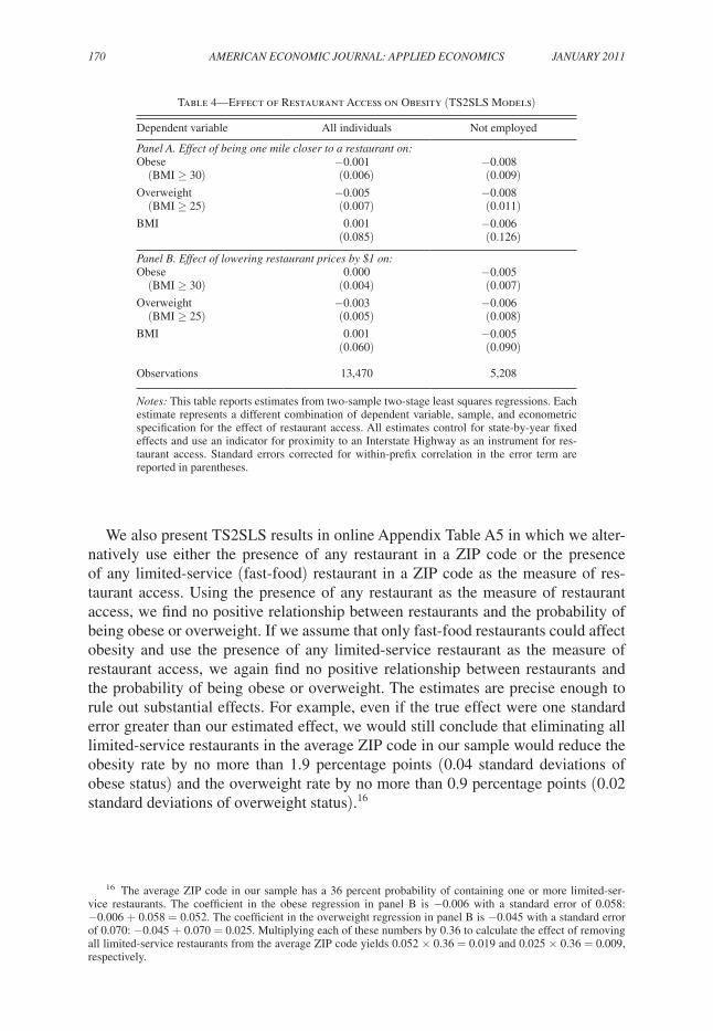
We also present TS2SLS results in online Appendix Table A5 in which we alter-natively use either the presence of any restaurant in a ZIP code or the presence of any limited-service (fast-food) restaurant in a ZIP code as the measure of res-taurant access. Using the presence of any restaurant as the measure of restaurant access, we find no positive relationship between restaurants and the probability of being obese or overweight. If we assume that only fast-food restaurants could affect obesity and use the presence of any limited-service restaurant as the measure of restaurant access, we again find no positive relationship between restaurants and the probability of being obese or overweight. The estimates are precise enough to rule out substantial effects. For example, even if the true effect were one standard error greater than our estimated effect, we would still conclude that eliminating all limited-service restaurants in the average ZIP code in our sample would reduce the obesity rate by no more than 1.9 percentage points (0.04 standard deviations of obese status) and the overweight rate by no more than 0.9 percentage points (0.02 standard deviations of overweight status).16
16 The average ZIP code in our sample has a 36 percent probability of containing one or more limited-ser-vice restaurants. The coefficient in the obese regression in panel B is −0.006 with a standard error of 0.058: −0.006 + 0.058 = 0.052. The coefficient in the overweight regression in panel B is −0.045 with a standard error of 0.070: −0.045 + 0.070 = 0.025. Multiplying each of these numbers by 0.36 to calculate the effect of removing all limited-service restaurants from the average ZIP code yields 0.052 × 0.36 = 0.019 and 0.025 × 0.36 = 0.009, respectively.
Table 4—Effect of Restaurant Access on Obesity (TS2SLS Models)
Dependent variable All individuals Not employed
panel A. Effect of being one mile closer to a restaurant on:Obese −0.001 −0.008 (BMI ≥ 30) (0.006) (0.009)Overweight −0.005 −0.008 (BMI ≥ 25) (0.007) (0.011)BMI 0.001 −0.006
(0.085) (0.126)
panel B. Effect of lowering restaurant prices by $1 on:Obese 0.000 −0.005 (BMI ≥ 30) (0.004) (0.007)Overweight −0.003 −0.006 (BMI ≥ 25) (0.005) (0.008)BMI 0.001 −0.005
(0.060) (0.090)
Observations 13,470 5,208
Notes: This table reports estimates from two-sample two-stage least squares regressions. Each estimate represents a different combination of dependent variable, sample, and econometric specification for the effect of restaurant access. All estimates control for state-by-year fixed effects and use an indicator for proximity to an Interstate Highway as an instrument for res-taurant access. Standard errors corrected for within-prefix correlation in the error term are reported in parentheses.
VoL. 3 No. 1 171ANdErSoN ANd MAtSA: ArE rEStAurANtS rEALLy SupErSIzINg AMErICA?
IV. Analysis of Alternative Interpretations
The clear null relationship between Interstate proximity and body mass suggests that the availability of restaurants does not affect obesity. However, there are sev-eral alternative explanations for the null relationship that merit consideration. First, although Interstate proximity correlates with restaurant availability, it is possible that the instrument has no effect on the frequency of restaurant consumption (formally, this is equivalent to an absence of the necessary first-stage relationship). Second, residents of towns adjacent to the highway may differ from residents in nonadjacent towns along dimensions that affect body mass. In that case, it is possible that a posi-tive effect of restaurants on body mass is masked by negative effects of other factors on body mass (formally, this is equivalent to a failure of the IV exclusion restric-tion). In this section, we analyze these two possibilities in detail.
A third possibility is that subtle forms of measurement error may attenuate the reduced form relationship between body mass and Interstate proximity in spite of a significant relationship between restaurant access and Interstate proximity. Online Appendix E explores this hypothesis in detail and concludes that measurement error cannot explain our results.
A. does Highway proximity Increase restaurant Consumption?
The first-stage relation estimated in Section IIIA demonstrates that residents of nonadjacent towns live significantly farther from their nearest restaurant than residents of adjacent towns. But does this difference actually affect restaurant consumption? Restaurant demand, for example, might be highly inelastic with respect to travel dis-tance, or optimizing consumers might choose to eat in a restaurant on days when they already travel to restaurant towns for other reasons. To validate the first-stage relation-ship between highway proximity and restaurant consumption, we conducted an origi-nal survey in a rural area that is representative of our study population. We surveyed customers at every fast-food restaurant lying within a 3,000 square-mile corridor of Interstate 5 in northern California. Logistical constraints compelled us to focus the survey on fast-food restaurants. However, fast-food meals comprise almost two-thirds of all meals consumed away from home (US Census Bureau 2005) and are presented in the obesity literature as being particularly unhealthy.17 These data reveal that high-way and restaurant proximity have strong effects on frequency of consumption.
The area of northern California that we analyze is approximately two-thirds the size of Connecticut. Centered on Interstate 5 (I-5) between Dunnigan and Corning, California, the study area is approximately 80 miles long and 40 miles wide and contains 23 fast-food restaurants, including McDonald’s, Burger King, Carl’s Jr., Jack in the Box, Taco Bell, KFC, Quiznos, and Subway. We chose this area because
17 We experimented with also surveying full-service restaurant customers, but the customer flows at full-ser-vice restaurants were so low that it was logistically infeasible to collect a sufficient number of responses. The results from the restaurant survey imply that fast-food consumption increases with Interstate proximity. Given these results, it is likely that full-service restaurant consumption increases with Interstate proximity as well. We perform robustness checks, described later in this section, to ensure that our results cannot be due to consumers substituting consumption to nonsurveyed full-service restaurants.

172 AMErICAN ECoNoMIC JourNAL: AppLIEd ECoNoMICS JANuAry 2011
it was the only continuous Interstate corridor with comparable population density to our main analytic sample located within a 200-mile radius of either Berkeley, CA, or Evanston, IL. Over 11 nonconsecutive days in June and July 2008, we approached 2,040 customers at all of these 23 restaurants and asked for their town and ZIP code of residence. Ninety-three percent of those approached responded to our short oral survey. Further details regarding the survey are presented in online Appendix F.
Using these data and ZIP code populations from the US Census, we estimate the relative frequency of fast-food consumption for each ZIP code in the study area. The sampling scheme for these data is different than for the census or BRFSS data since we sample at the point of consumption (the restaurant) rather than at the point of resi-dence (the ZIP code or telephone exchange area). Nevertheless, because we sample from the entire universe of restaurants in the study area, both schemes should produce similar estimates of per capita fast-food consumption (up to sampling error). As an example, suppose that we wish to measure the number of California residents and Nevada residents who attended the 2009 annual meeting of the American Economic Association (AEA) in San Francisco. One alternative would be to telephone a random sample of California and Nevada residents and ask, “Did you register for and attend the 2009 AEA annual meeting?” The other alternative would be to stand at the AEA registration desk and ask each person who registers, “What state are you from?” Both alternatives are valid and would yield the same answer asymptotically. Logistically, however, in both the AEA scenario and our actual survey, it is far less expensive to gather an equivalent number of observations using a direct customer survey than a telephone survey. For this reason, we conduct a direct customer survey. The two meth-ods will produce different results only if we fail to capture a representative sample of the universe of restaurants, either spatially or temporally. (In the AEA scenario, the direct survey might fail if it only covered one of multiple registration desks or if it only sampled conference attendees from 8 a.m. to 12 p.m. These issues would result in bias if California and Nevada residents were more or less likely to use a particular registra-tion desk or to arrive in the afternoon.) Robustness checks, described below, indicate that neither of these issues affects our results.
Table 5 presents summary statistics for the survey area and for the main ana-lytic sample used in Section III. The survey area is more racially diverse, younger, less educated, and less wealthy than the average ZIP code in our BRFSS sample. Because the effect of highways on obesity does not vary by demographic group (see Online Appendix Table A3), we do not expect these differences to bias our conclu-sions. ZIP codes in the survey area are also 10 to 16 percentage points more likely to contain some type of restaurant than the average ZIP code in our main study.
The first-stage relationship between highway proximity and restaurant access is roughly similar in the survey area and in our main study. For example, highway proximity increases the likelihood of having a restaurant by 21 percentage points in the survey area and 17.5 percentage points in our main analytic sample. Highway proximity reduces the average distance to travel to the nearest restaurant by 2.05 miles in the survey area and 1.50 miles in our main analytic sample.
The survey data indicate that restaurants located in towns adjacent to the highway are much more likely to serve long-distance travelers than restaurants located in non-adjacent towns. Fifty percent of customers in adjacent restaurants live more than one

VoL. 3 No. 1 173ANdErSoN ANd MAtSA: ArE rEStAurANtS rEALLy SupErSIzINg AMErICA?
hour from the restaurant (as measured by Google Maps), compared to only 17 percent of customers in nonadjacent restaurants. This differential is statistically significant (t = 6.8) and supports the idea that restaurant density is greater adjacent to highways because these areas have greater demand from highway travelers passing through.
The relationship between the frequency of fast-food consumption and highway proximity is economically and statistically significant. Residents of towns located 0–5 miles from I-5 visit restaurants at a rate of 128 daily visits per 1,000 residents.18 Residents of towns located 5–10 miles from I-5 visit restaurants at a rate of 68 daily visits per 1,000 residents.19 This 47 percent decrease in frequency of fast-food consumption is highly significant (t = 8.4) and robust to the choice of sampling weights.20 The relationship between fast-food consumption and restaurant proximity is also strong and statistically significant. Residents of towns that contain a fast-food restaurant visit restaurants at a rate of 127 daily visits per 1,000 residents, while
18 To convert our survey results to daily visit rates, we multiply by the ratio of business hours divided by sur-veyed hours. Business hours are assumed to start at 7 a.m. and end at 10 p.m., while surveyed hours began at 11 a.m. and ended by 8 p.m. If the average store is busier during the afternoon and evening than during the morning and late at night, then daily rates may be overstated. However, because the same multiplication factor is applied to the results from all towns, the conclusions of this section (which focus on relative comparisons between towns) are unaffected by the choice of multiplier.
19 In theory, households in off-highway ZIP codes could send a single household member to bring back food for multiple household members. In this case, the number of people visiting fast-food restaurants from these ZIP codes would appear to be low, but the number of parties (i.e., distinct groups of customers) visiting fast-food restaurants from these ZIP codes would not appear to be low. Our data cast doubt on this possibility: the relative differential between highway and nonhighway ZIP codes is identical if we perform the analysis using parties per 1,000 resi-dents instead of people per 1,000 residents.
20 Each fast-food restaurant is sampled on at least one weekday and one weekend day, but logistical constraints led some restaurants to be sampled for longer durations than others. The sampling weights account for these dif-ferences by reweighting the data in proportion to the inverse of the hours surveyed per restaurant. The results are not sensitive to the exact choice of weights. For example, even when making no adjustments at all for sampling duration, we find that fast-food consumption decreases by 40 percent in nonadjacent towns relative to adjacent towns (t = 6.8).
Table 5—Summary Statistics
Northern California study area Main analytic sample
Mean SDSample
size Mean SDSample
size
White 0.69 0.19 26 0.93 0.10 551Under 21 0.35 0.06 26 0.31 0.05 551Over 65 0.12 0.04 26 0.16 0.05 551College 0.36 0.12 25 0.43 0.13 551Median household income $31,653 $9,243 26 $34,689 $7,728 551Any restaurant 0.77 0.43 26 0.61 0.49 551Any full-service restaurant 0.65 0.49 26 0.55 0.50 551Any limited-service restaurant 0.46 0.51 26 0.36 0.48 551Number of full-service restaurants 2.85 3.90 26 2.38 4.83 551Number of limited-service restaurants 2.04 3.01 26 1.64 3.51 551
Notes: This table reports unweighted summary statistics for the rural northern California survey area (used in Section IVA) and the main analytic sample (used in Section III). The rural northern California survey area con-sists of the 26 ZIP codes lying within 20 miles of the I-5 corridor from Dunnigan to Corning, CA. The analytic sample consists of all ZIP codes in Arkansas, Colorado, Iowa, Kansas, Maine, Missouri, North Dakota, Nebraska, Oklahoma, Utah, and Vermont that are located less than 10 miles from an Interstate Highway, more than 30 miles from an urban area, and have a population density of less than 80 persons per square mile. All data are from the cen-sus, and standard deviations are calculated at the ZIP code level.
174 AMErICAN ECoNoMIC JourNAL: AppLIEd ECoNoMICS JANuAry 2011
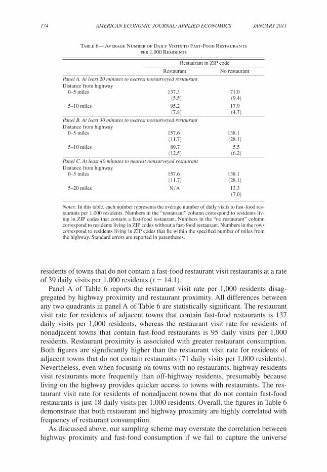
residents of towns that do not contain a fast-food restaurant visit restaurants at a rate of 39 daily visits per 1,000 residents (t = 14.1).
Panel A of Table 6 reports the restaurant visit rate per 1,000 residents disag-gregated by highway proximity and restaurant proximity. All differences between any two quadrants in panel A of Table 6 are statistically significant. The restaurant visit rate for residents of adjacent towns that contain fast-food restaurants is 137 daily visits per 1,000 residents, whereas the restaurant visit rate for residents of nonadjacent towns that contain fast-food restaurants is 95 daily visits per 1,000 residents. Restaurant proximity is associated with greater restaurant consumption. Both figures are significantly higher than the restaurant visit rate for residents of adjacent towns that do not contain restaurants (71 daily visits per 1,000 residents). Nevertheless, even when focusing on towns with no restaurants, highway residents visit restaurants more frequently than off-highway residents, presumably because living on the highway provides quicker access to towns with restaurants. The res-taurant visit rate for residents of nonadjacent towns that do not contain fast-food restaurants is just 18 daily visits per 1,000 residents. Overall, the figures in Table 6 demonstrate that both restaurant and highway proximity are highly correlated with frequency of restaurant consumption.
As discussed above, our sampling scheme may overstate the correlation between highway proximity and fast-food consumption if we fail to capture the universe
Table 6— Average Number of Daily Visits to Fast-Food Restaurants per 1,000 Residents
Restaurant in ZIP code
Restaurant No restaurant
panel A. At least 20 minutes to nearest nonsurveyed restaurantDistance from highway 0–5 miles 137.3 71.0
(5.5) (9.4) 5–10 miles 95.2 17.9
(7.8) (4.7)panel B. At least 30 minutes to nearest nonsurveyed restaurantDistance from highway 0–5 miles 157.6 138.1
(11.7) (28.1) 5–10 miles 89.7 5.5
(12.5) (6.2)panel C. At least 40 minutes to nearest nonsurveyed restaurantDistance from highway 0–5 miles 157.6 138.1
(11.7) (28.1) 5–20 miles N/A 13.3
(7.0)
Notes: In this table, each number represents the average number of daily visits to fast-food res-taurants per 1,000 residents. Numbers in the “restaurant” column correspond to residents liv-ing in ZIP codes that contain a fast-food restaurant. Numbers in the “no restaurant” column correspond to residents living in ZIP codes without a fast-food restaurant. Numbers in the rows correspond to residents living in ZIP codes that lie within the specified number of miles from the highway. Standard errors are reported in parentheses.
VoL. 3 No. 1 175ANdErSoN ANd MAtSA: ArE rEStAurANtS rEALLy SupErSIzINg AMErICA?
of fast-food restaurants, either temporally or spatially. Temporally, we may fail to appropriately measure the universe of restaurant consumption if relative visit rates differ throughout the day, because we only sample from the beginning of lunchtime until the end of dinnertime (11 a.m.–8 p.m.). If off-highway residents eat a dispro-portionate number of their fast-food meals during breakfast hours, then we may be overstating the relationship between highway proximity and fast-food consump-tion. Breakfast accounts for 11 percent of fast-food meals (US Census Bureau 2005, 69). We assess the robustness of our results by assuming that off-highway residents consume fast-food breakfasts at double the implied rate from our survey. Under this assumption, the fast-food consumption rate of off-highway residents is still 41 percent lower than that of on-highway residents.21
In the spatial dimension, we may fail to capture the universe of fast-food restau-rant consumption because we do not sample every fast-food restaurant in the state of California. Instead, the estimates reported above assume that consumers do not travel more than 20 minutes to obtain fast food (more precisely, there is no difference in con-sumption rates between on- and off-highway residents at that distance). For residents of the ZIP codes analyzed in Table 6, the driving time to the nearest nonsurveyed fast-food restaurant ranges from 21 minutes to 48 minutes. We check the sensitivity of our results to the 20-minute cutoff by re-estimating them on samples in which we restrict the sample based on the driving time to the nearest nonsurveyed fast-food restaurant. If patronage of nonsurveyed restaurants is driving the on-highway/off-highway con-sumption differential, then we should expect the differential to narrow as we increase the minimum driving time cutoff. Instead, we observe the opposite pattern.
When restricting the sample to ZIP codes in which residents must drive at least 30 minutes to reach the nearest nonsurveyed fast-food restaurant, the frequency of fast-food consumption of off-highway residents is 52 percent lower than that of on-highway residents (t = 5.4). The disaggregated results are presented in panel B of Table 6. When restricting the sample to ZIP codes in which residents must drive at least 40 minutes to reach the nearest nonsurveyed fast-food restaurant, the fre-quency of fast-food consumption of off-highway residents is 91 percent lower than that of on-highway residents. The disaggregated results, reported in panel C of Table 6, reveal that the large differential between on-highway and off-highway fast-food consumption arises because the off-highway sample now has no ZIP codes that contain restaurants.22 Restricting the sample to residents who live very far from the nearest nonsurveyed restaurant indicates that a failure to capture the entire universe of restaurants is not leading us to overstate the correlation between highway proxim-ity and fast-food consumption.23
21 Our survey implies that off-highway residents consume fast food at 53 percent of the rate of on-highway residents. Doubling this figure for breakfast implies that off-highway residents consume fast-food breakfasts at 2 × 53 = 106 percent of the rate of on-highway residents. Because breakfasts comprise 11 percent of fast-food meals, the relative fast-food consumption rate of off-highway versus on-highway residents is 0.53 × (89 percent of meals) + 1.06 × (11 percent of meals) = 0.59.
22 To maintain a reasonable sample size, we expand the off-highway group in panel C to contain all ZIP codes from 5 to 20 miles from I-5. Limiting the sample to ZIP codes between 5 to 10 miles generates qualitatively similar results.
23 Another possibility is that consumers in towns without fast-food restaurants perfectly substitute consumption to local full-service restaurants. However, in the restricted samples, for all but four towns, the closest full-service restaurant is no closer than the closest fast-food restaurant. Estimates from specifications that exclude residents
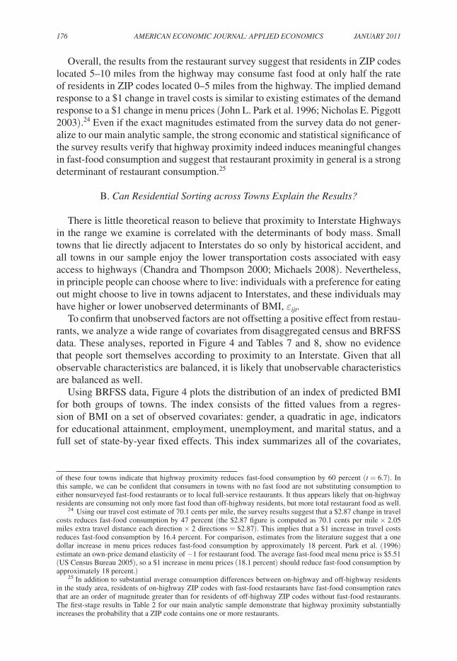
176 AMErICAN ECoNoMIC JourNAL: AppLIEd ECoNoMICS JANuAry 2011
Overall, the results from the restaurant survey suggest that residents in ZIP codes located 5–10 miles from the highway may consume fast food at only half the rate of residents in ZIP codes located 0–5 miles from the highway. The implied demand response to a $1 change in travel costs is similar to existing estimates of the demand response to a $1 change in menu prices (John L. Park et al. 1996; Nicholas E. Piggott 2003).24 Even if the exact magnitudes estimated from the survey data do not gener-alize to our main analytic sample, the strong economic and statistical significance of the survey results verify that highway proximity indeed induces meaningful changes in fast-food consumption and suggest that restaurant proximity in general is a strong determinant of restaurant consumption.25
B. Can residential Sorting across towns Explain the results?
There is little theoretical reason to believe that proximity to Interstate Highways in the range we examine is correlated with the determinants of body mass. Small towns that lie directly adjacent to Interstates do so only by historical accident, and all towns in our sample enjoy the lower transportation costs associated with easy access to highways (Chandra and Thompson 2000; Michaels 2008). Nevertheless, in principle people can choose where to live: individuals with a preference for eating out might choose to live in towns adjacent to Interstates, and these individuals may have higher or lower unobserved determinants of BMI, εijt.
To confirm that unobserved factors are not offsetting a positive effect from restau-rants, we analyze a wide range of covariates from disaggregated census and BRFSS data. These analyses, reported in Figure 4 and Tables 7 and 8, show no evidence that people sort themselves according to proximity to an Interstate. Given that all observable characteristics are balanced, it is likely that unobservable characteristics are balanced as well.
Using BRFSS data, Figure 4 plots the distribution of an index of predicted BMI for both groups of towns. The index consists of the fitted values from a regres-sion of BMI on a set of observed covariates: gender, a quadratic in age, indicators for educational attainment, employment, unemployment, and marital status, and a full set of state-by-year fixed effects. This index summarizes all of the covariates,
of these four towns indicate that highway proximity reduces fast-food consumption by 60 percent (t = 6.7). In this sample, we can be confident that consumers in towns with no fast food are not substituting consumption to either nonsurveyed fast-food restaurants or to local full-service restaurants. It thus appears likely that on-highway residents are consuming not only more fast food than off-highway residents, but more total restaurant food as well.
24 Using our travel cost estimate of 70.1 cents per mile, the survey results suggest that a $2.87 change in travel costs reduces fast-food consumption by 47 percent (the $2.87 figure is computed as 70.1 cents per mile × 2.05 miles extra travel distance each direction × 2 directions = $2.87). This implies that a $1 increase in travel costs reduces fast-food consumption by 16.4 percent. For comparison, estimates from the literature suggest that a one dollar increase in menu prices reduces fast-food consumption by approximately 18 percent. Park et al. (1996) estimate an own-price demand elasticity of −1 for restaurant food. The average fast-food meal menu price is $5.51 (US Census Bureau 2005), so a $1 increase in menu prices (18.1 percent) should reduce fast-food consumption by approximately 18 percent.)
25 In addition to substantial average consumption differences between on-highway and off-highway residents in the study area, residents of on-highway ZIP codes with fast-food restaurants have fast-food consumption rates that are an order of magnitude greater than for residents of off-highway ZIP codes without fast-food restaurants. The first-stage results in Table 2 for our main analytic sample demonstrate that highway proximity substantially increases the probability that a ZIP code contains one or more restaurants.
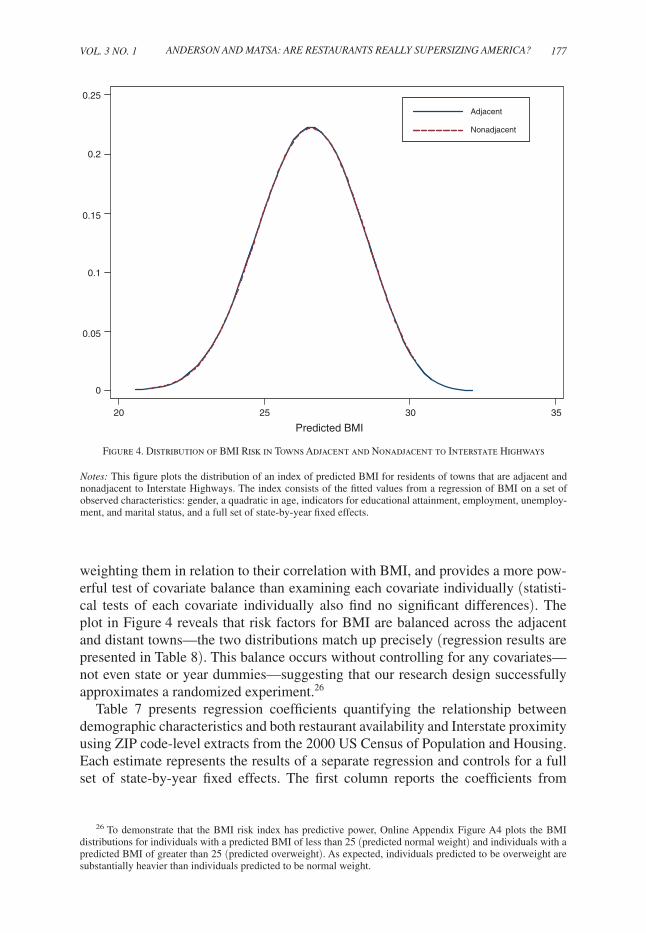
VoL. 3 No. 1 177ANdErSoN ANd MAtSA: ArE rEStAurANtS rEALLy SupErSIzINg AMErICA?
weighting them in relation to their correlation with BMI, and provides a more pow-erful test of covariate balance than examining each covariate individually (statisti-cal tests of each covariate individually also find no significant differences). The plot in Figure 4 reveals that risk factors for BMI are balanced across the adjacent and distant towns—the two distributions match up precisely (regression results are presented in Table 8). This balance occurs without controlling for any covariates—not even state or year dummies—suggesting that our research design successfully approximates a randomized experiment.26
Table 7 presents regression coefficients quantifying the relationship between demographic characteristics and both restaurant availability and Interstate proximity using ZIP code-level extracts from the 2000 US Census of Population and Housing. Each estimate represents the results of a separate regression and controls for a full set of state-by-year fixed effects. The first column reports the coefficients from
26 To demonstrate that the BMI risk index has predictive power, Online Appendix Figure A4 plots the BMI distributions for individuals with a predicted BMI of less than 25 (predicted normal weight) and individuals with a predicted BMI of greater than 25 (predicted overweight). As expected, individuals predicted to be overweight are substantially heavier than individuals predicted to be normal weight.
0.25
Adjacent
0.15
0.2
Nonadjacent
0.05
0.1
0
20 25 30 35
Predicted BMI
Figure 4. Distribution of BMI Risk in Towns Adjacent and Nonadjacent to Interstate Highways
Notes: This figure plots the distribution of an index of predicted BMI for residents of towns that are adjacent and nonadjacent to Interstate Highways. The index consists of the fitted values from a regression of BMI on a set of observed characteristics: gender, a quadratic in age, indicators for educational attainment, employment, unemploy-ment, and marital status, and a full set of state-by-year fixed effects.

178 AMErICAN ECoNoMIC JourNAL: AppLIEd ECoNoMICS JANuAry 2011
regressions that run different dependent variables on an indicator that is unity if a ZIP code contains any restaurants and zero otherwise. This sample contains all ZIP codes in the states that we study. ZIP codes with restaurants contain a disproportion-ate number of females and minorities, and their residents tend to be better educated with higher incomes. These estimates are statistically significant, with t-statistics ranging from 9.0 to 20.3. The results indicate that restaurant placement in the full sample of ZIP codes is strongly correlated with other factors that may affect obesity.
The second column of Table 7 reports the coefficients from a series of regres-sions running the same dependent variables on the instrument, proximity to an Interstate Highway. This sample contains only rural ZIP codes lying within 10 miles of an Interstate Highway (the analytic sample). In contrast to the first column, no regression returns a statistically significant coefficient. More important, the lack of statistical significance occurs because of a sharp drop in the magnitude of the coefficients, not because of an increase in the standard errors. Relative to the first column, coefficient magnitudes decrease by factors ranging from 3 to 94 times, with an average decrease in magnitude of 27.9 times. Overall, important demographic characteristics seem to be well balanced across areas that are adjacent and nonadja-cent to Interstate Highways.
Table 8 presents similar results using individual-level BRFSS data. These results reinforce the conclusion that the instrument is uncorrelated with other determinants of BMI. The “BMI risk index” consists of the fitted values from a regression of BMI on
Table 7— ZIP Code-Level Covariate Balance
Dependent variable Near restaurant Near interstate
Percent male −0.009 −0.003(0.001) (0.002)
Percent white −0.039 −0.001(0.003) (0.007)
Percent under 21 −0.0015 −0.0001(0.0015) (0.0038)
Percent over 65 −0.0017 −0.0004(0.0014) (0.0037)
Percent with some college or more 0.061 0.002(0.003) (0.009)
Median household income 2,736 29(253) (593)
State-by-year fixed effects Yes Yes
Sample: Description Full sample Analytic sample Number of ZIP codes 7,105 551
Notes: In this table, each coefficient represents a separate regression, rows correspond to differ-ent dependent variables, and columns correspond to different samples of ZIP codes and regres-sion specifications. All regressions contain state-by-year fixed effects, and robust standard errors are reported in parentheses. In the first column (“near restaurant”), the reported coef-ficients are from regressions of the specified dependent variables on an indicator variable for whether a ZIP code contains one or more restaurants; estimates in this column are based on a full sample of ZIP codes in the states represented in the analytic sample. In the second column (“near interstate”), the reported coefficients are from regressions of the specified dependent variables on an indicator variable for whether a ZIP code is adjacent to an Interstate Highway; estimates in this column are based on the analytic sample (defined in the note to Table 1).

VoL. 3 No. 1 179ANdErSoN ANd MAtSA: ArE rEStAurANtS rEALLy SupErSIzINg AMErICA?
a set of observed covariates, as defined above in the context of Figure 4. The effect of the instrument on the BMI risk index is statistically and economically insignificant; the coefficient of −0.038 corresponds to less than 0.01 standard deviations of BMI. The “obese risk index” and the “overweight risk index” are constructed similarly to the BMI Risk Index, but the covariates are used to predict obese status or overweight status rather than BMI. There is no statistically or economically significant relation-ship between either index and proximity to an Interstate Highway.
Some states included additional variables in the BRFSS extracts they provided. We do not include these variables when estimating the BMI, obese, or overweight risk indices because doing so would severely reduce our sample size. However, indi-vidual tests for each variable also support the validity of our identification strategy. Regression estimates for these additional variables are presented in the last five rows of Table 8. There is no significant relationship between proximity to an Interstate and average income, smoking rates, or height. More important, individuals living in towns adjacent to and nonadjacent to an Interstate have similar desired weights and exer-cise with similar frequency. All of the regression coefficients imply correlations that are not only statistically insignificant, but also economically insignificant.27 Based on
27 Interstate proximity is negatively correlated with income and smoking, although neither of these differ-ences is statistically significant. Both factors are believed to reduce body mass, so the negative correlation may in theory bias our estimator toward finding a positive effect of Interstate proximity (and thus restaurants) on
Table 8—Individual-Level Covariate Balance
Dependent variable Coefficient Sample size
BMI risk index −0.038 12,797(0.029)
Obese (BMI ≥ 30) −0.0019 12,797 risk index (0.0016)Overweight (BMI ≥ 25) −0.0037 12,797 risk index (0.0031)Average income ($) −482 10,560
(936)Ever smoked −0.019 9,180
(0.012)Height (in cm) −0.010 13,470
(0.182)Desired weight (in kg) −0.280 4,154
(0.425)Exercised in last month 0.012 6,731
(0.016)
State-by-year fixed effects Yes
Notes: In this table, each coefficient represents a separate regression. The reported coeffi-cients are from regressions of the specified dependent variables on an indicator for whether the respondent’s telephone prefix is adjacent to an Interstate Highway. All regressions contain state-by-year fixed effects. Standard errors corrected for within-prefix correlation in the error term are reported in parentheses. The BMI (obese, overweight) Risk Index consists of the fit-ted values from a regression of BMI (obese, overweight) on a set of observed covariates: gen-der, a quadratic in age, indicators for educational attainment, employment, unemployment, and marital status, and a full set of state-by-year fixed effects.

180 AMErICAN ECoNoMIC JourNAL: AppLIEd ECoNoMICS JANuAry 2011
these analyses, we conclude that there is no evidence of selection across adjacent and nonadjacent towns.
V. Why Don’t Restaurants Affect Obesity?
Given the established correlation between eating out and obesity, as well as the simple fact that restaurant portions have grown markedly over the past several decades, it may appear surprising that restaurant consumption has no causal effect on obesity. To reconcile these facts, this section presents analysis of the causal mechanisms behind the limited effect of restaurants on obesity. As illustrated by the theoretical framework developed in Section I, there are two possible reasons why varying the effective price of restaurants would not affect body weight. First, after accounting for selection based on caloric demand, individuals may not consume substantially more calories when they eat out than they do at home. Second, even if people do consume more calories at restaurants, they may offset the additional res-taurant consumption by eating less during the rest of the day. To explore the empiri-cal relevance of these potential mechanisms, we examine food intake data collected by the US Department of Agriculture.
The food intake data come from the Continuing Survey of Food Intake by Individuals, conducted from 1994 through 1996. These data include detailed information about all of the food items consumed by several thousand adults over two nonconsecutive days. We focus our analysis on obese and overweight individuals who live outside of metro-politan areas because they are more representative of the subjects in our instrumental variables analysis.28 We also drop a small number of observations with obvious cod-ing errors, leaving an analytic sample of 854 individuals. Some individuals in nutri-tion studies likely underreport the amount of food they eat either because they forget or because they intentionally misreport (Sheila A. Bingham 1987; Dale A. Schoeller 1990; Walter Mertz et al. 1991). The survey instrument may also under- or overesti-mate caloric intake from some respondents’ descriptions of what they eat. Although simple estimates of caloric intake may be affected by such reporting errors, our ulti-mate conclusions are based on relative comparisons of (1) between-individual and within-individual estimators and (2) meal-level and daily-level estimators. The pres-ence of some misreporting is unlikely to affect these relative comparisons.
Respondents reported eating at a restaurant about once every three days. On days when survey respondents reported eating “more than usual,” they were asked to explain why. The most popular reasons for eating more than usual were a social occasion or special day (5.4 percent of days) and because they were hungrier (1.3 percent of days). On only five out of every 1,000 days did people report eating more because they had eaten at a restaurant. These responses suggest that eating out does not actually increase
obesity. The −0.28 coefficient estimate for desired weight implies a difference in desired BMI of 0.09 BMI points for an individual of average height (5 feet 7 inches); this effect is less than 0.02 standard deviations of BMI. The 0.012 coefficient estimate for exercised in the last month represents only a 1.6 percent reduction, relative to the mean.
28 We focus on obese and overweight individuals because we are interested in how restaurants affect the preva-lence of obesity. By definition, restaurants do not cause obesity among individuals that maintain a normal weight. Expanding the sample, however, to include all geographic areas and/or nonoverweight individuals increases the sample size to 5,713 individuals and leads to similar conclusions (see Online Appendix Table A6).
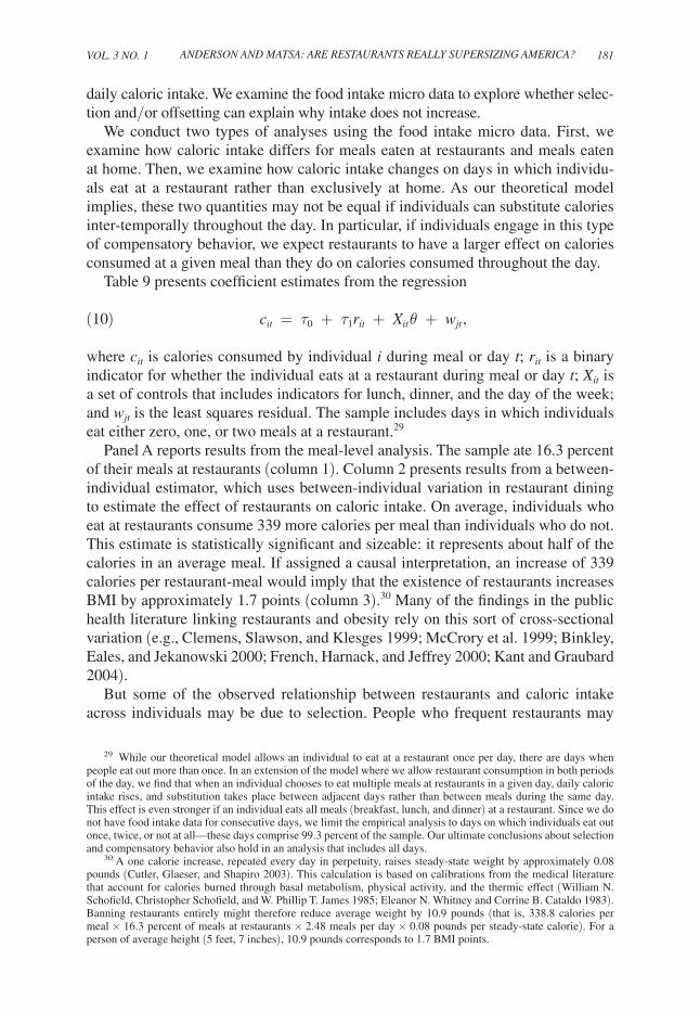
VoL. 3 No. 1 181ANdErSoN ANd MAtSA: ArE rEStAurANtS rEALLy SupErSIzINg AMErICA?
daily caloric intake. We examine the food intake micro data to explore whether selec-tion and/or offsetting can explain why intake does not increase.
We conduct two types of analyses using the food intake micro data. First, we examine how caloric intake differs for meals eaten at restaurants and meals eaten at home. Then, we examine how caloric intake changes on days in which individu-als eat at a restaurant rather than exclusively at home. As our theoretical model implies, these two quantities may not be equal if individuals can substitute calories inter-temporally throughout the day. In particular, if individuals engage in this type of compensatory behavior, we expect restaurants to have a larger effect on calories consumed at a given meal than they do on calories consumed throughout the day.
Table 9 presents coefficient estimates from the regression
(10) cit = τ0 + τ1rit + Xit θ + wjt ,
where cit is calories consumed by individual i during meal or day t; rit is a binary indicator for whether the individual eats at a restaurant during meal or day t; Xit is a set of controls that includes indicators for lunch, dinner, and the day of the week; and wjt is the least squares residual. The sample includes days in which individuals eat either zero, one, or two meals at a restaurant.29
Panel A reports results from the meal-level analysis. The sample ate 16.3 percent of their meals at restaurants (column 1). Column 2 presents results from a between-individual estimator, which uses between-individual variation in restaurant dining to estimate the effect of restaurants on caloric intake. On average, individuals who eat at restaurants consume 339 more calories per meal than individuals who do not. This estimate is statistically significant and sizeable: it represents about half of the calories in an average meal. If assigned a causal interpretation, an increase of 339 calories per restaurant-meal would imply that the existence of restaurants increases BMI by approximately 1.7 points (column 3).30 Many of the findings in the public health literature linking restaurants and obesity rely on this sort of cross-sectional variation (e.g., Clemens, Slawson, and Klesges 1999; McCrory et al. 1999; Binkley, Eales, and Jekanowski 2000; French, Harnack, and Jeffrey 2000; Kant and Graubard 2004).
But some of the observed relationship between restaurants and caloric intake across individuals may be due to selection. People who frequent restaurants may
29 While our theoretical model allows an individual to eat at a restaurant once per day, there are days when people eat out more than once. In an extension of the model where we allow restaurant consumption in both periods of the day, we find that when an individual chooses to eat multiple meals at restaurants in a given day, daily caloric intake rises, and substitution takes place between adjacent days rather than between meals during the same day. This effect is even stronger if an individual eats all meals (breakfast, lunch, and dinner) at a restaurant. Since we do not have food intake data for consecutive days, we limit the empirical analysis to days on which individuals eat out once, twice, or not at all—these days comprise 99.3 percent of the sample. Our ultimate conclusions about selection and compensatory behavior also hold in an analysis that includes all days.
30 A one calorie increase, repeated every day in perpetuity, raises steady-state weight by approximately 0.08 pounds (Cutler, Glaeser, and Shapiro 2003). This calculation is based on calibrations from the medical literature that account for calories burned through basal metabolism, physical activity, and the thermic effect (William N. Schofield, Christopher Schofield, and W. Phillip T. James 1985; Eleanor N. Whitney and Corrine B. Cataldo 1983). Banning restaurants entirely might therefore reduce average weight by 10.9 pounds (that is, 338.8 calories per meal × 16.3 percent of meals at restaurants × 2.48 meals per day × 0.08 pounds per steady-state calorie). For a person of average height (5 feet, 7 inches), 10.9 pounds corresponds to 1.7 BMI points.
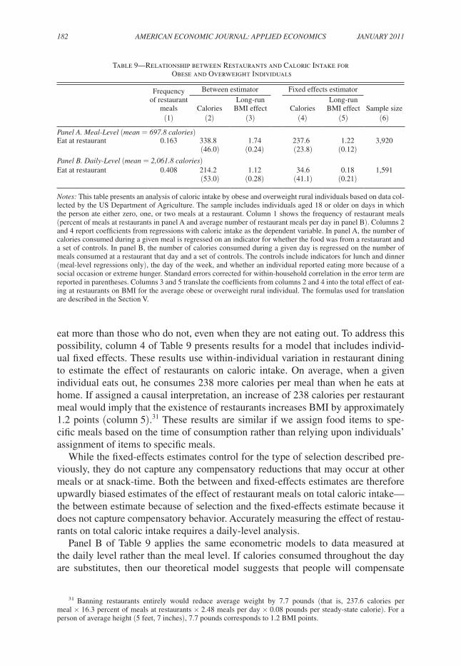
182 AMErICAN ECoNoMIC JourNAL: AppLIEd ECoNoMICS JANuAry 2011
eat more than those who do not, even when they are not eating out. To address this possibility, column 4 of Table 9 presents results for a model that includes individ-ual fixed effects. These results use within-individual variation in restaurant dining to estimate the effect of restaurants on caloric intake. On average, when a given individual eats out, he consumes 238 more calories per meal than when he eats at home. If assigned a causal interpretation, an increase of 238 calories per restaurant meal would imply that the existence of restaurants increases BMI by approximately 1.2 points (column 5).31 These results are similar if we assign food items to spe-cific meals based on the time of consumption rather than relying upon individuals’ assignment of items to specific meals.
While the fixed-effects estimates control for the type of selection described pre-viously, they do not capture any compensatory reductions that may occur at other meals or at snack-time. Both the between and fixed-effects estimates are therefore upwardly biased estimates of the effect of restaurant meals on total caloric intake—the between estimate because of selection and the fixed-effects estimate because it does not capture compensatory behavior. Accurately measuring the effect of restau-rants on total caloric intake requires a daily-level analysis.
Panel B of Table 9 applies the same econometric models to data measured at the daily level rather than the meal level. If calories consumed throughout the day are substitutes, then our theoretical model suggests that people will compensate
31 Banning restaurants entirely would reduce average weight by 7.7 pounds (that is, 237.6 calories per meal × 16.3 percent of meals at restaurants × 2.48 meals per day × 0.08 pounds per steady-state calorie). For a person of average height (5 feet, 7 inches), 7.7 pounds corresponds to 1.2 BMI points.
Table 9—Relationship between Restaurants and Caloric Intake for Obese and Overweight Individuals
Frequency of restaurant
meals
Between estimator Fixed effects estimator
CaloriesLong-run
BMI effect CaloriesLong-run
BMI effect Sample size(1) (2) (3) (4) (5) (6)
panel A. Meal-Level (mean = 697.8 calories)Eat at restaurant 0.163 338.8 1.74 237.6 1.22 3,920
(46.0) (0.24) (23.8) (0.12)panel B. daily-Level (mean = 2,061.8 calories)Eat at restaurant 0.408 214.2 1.12 34.6 0.18 1,591
(53.0) (0.28) (41.1) (0.21)
Notes: This table presents an analysis of caloric intake by obese and overweight rural individuals based on data col-lected by the US Department of Agriculture. The sample includes individuals aged 18 or older on days in which the person ate either zero, one, or two meals at a restaurant. Column 1 shows the frequency of restaurant meals (percent of meals at restaurants in panel A and average number of restaurant meals per day in panel B). Columns 2 and 4 report coefficients from regressions with caloric intake as the dependent variable. In panel A, the number of calories consumed during a given meal is regressed on an indicator for whether the food was from a restaurant and a set of controls. In panel B, the number of calories consumed during a given day is regressed on the number of meals consumed at a restaurant that day and a set of controls. The controls include indicators for lunch and dinner (meal-level regressions only), the day of the week, and whether an individual reported eating more because of a social occasion or extreme hunger. Standard errors corrected for within-household correlation in the error term are reported in parentheses. Columns 3 and 5 translate the coefficients from columns 2 and 4 into the total effect of eat-ing at restaurants on BMI for the average obese or overweight rural individual. The formulas used for translation are described in the Section V.

VoL. 3 No. 1 183ANdErSoN ANd MAtSA: ArE rEStAurANtS rEALLy SupErSIzINg AMErICA?
for larger portions at restaurants by consuming less throughout the rest of the day. Consistent with this prediction, the coefficient in the daily-level fixed-effects regres-sion is substantially less than the corresponding estimate at the meal level. In fact, eating out increases intake over the entire day by only 35 calories—compared to an average daily caloric intake of 2,062 calories. Column 5 translates the coefficient into the long-term effect on BMI—an increase of 35 calories per restaurant meal implies that the existence of restaurants increases BMI by less than 0.2 points.32 This effect is statistically insignificant and represents a decline of almost 90 percent from the between-individual meal-level estimate. The result suggests that, although individuals tend to eat more at restaurants, they compensate to a substantial degree by eating less throughout the rest of the day. Meal-level estimates therefore overes-timate the net effect of restaurants on total caloric intake.
The between-individual coefficient, presented in column 2, is significantly larger than the fixed-effects coefficient (214 versus 35), implying that individuals who fre-quent restaurants also eat more at home. This difference suggests that selection may explain why a number of observational studies have found a link between caloric intake and food away from home. Of course, even with individual fixed effects, the decision to eat at a restaurant is not exogenous. Given the size of restaurant portions, we suspect that consumers tend to eat at restaurants on days when they are espe-cially hungry. The 35-calorie-per-meal fixed-effects estimate therefore represents an upper bound and implies that restaurant meals do not have a substantive causal effect on total caloric intake.
The food intake results suggest that banning restaurants entirely would reduce BMI by less than 0.2 points. This effect is economically insignificant—it repre-sents 0.03 standard deviations of BMI. Banning restaurants entirely, however, is an unrealistic policy. More practical public policies would have smaller effects; for example, reducing restaurant consumption by 25 percent would reduce BMI by less than 0.05 points. These estimates are close to zero and match closely the instrumental variables estimates presented above in Table 4. They are also robust to various analytical extensions. We present implied BMI effects separately for overweight, obese, and all individuals in both rural areas and in all areas in Online Appendix Table A6 (these effects are calculated using the same methodology as the estimate reported in column 5, panel B of Table 9). In all cases, the BMI effects of completely banning restaurants represent less than 0.08 standard deviations of BMI. We also present BMI effects separately for full-service and fast-food restau-rants. There is no evidence that one type of restaurant is consistently associated with greater weight gain.
These conclusions are consistent with results on calorie offsetting from con-trolled laboratory and field experiments in which individuals are offered meals of varying caloric content. Subjects offered more caloric meals tend to compensate by eating less later in the day, while subjects offered less caloric meals compensate by eating more later in the day (Richard W. Foltin et al. 1990; Foltin et al. 1992; Clare
32 Banning restaurants entirely would reduce average weight by 1.1 pounds (that is, 34.6 calories per meal × 0.408 restaurant meals per day × 0.08 pounds per daily steady-state calorie). For a person of average height (5 feet, 7 inches), 1.1 pounds corresponds to 0.2 BMI points.

184 AMErICAN ECoNoMIC JourNAL: AppLIEd ECoNoMICS JANuAry 2011
L. Lawton et al. 1998). In other research, subjects encouraged to eat high-calorie sandwiches tend to compensate by choosing lower-calorie side dishes and drinks (Jessica Wisdom, Julia Downs, and George F. Loewenstein 2010). These behaviors may be rooted in physiological mechanisms identified by the medical literature on the epidemiology of obesity (see, for example, David E. Cummings and Michael W. Schwartz 2002). The human body is understood to have a physiological system that regulates body weight in a manner analogous to that by which a thermostat con-trols ambient temperature. Each individual’s target body weight is determined by a combination of genetic and environmental factors, and the body’s weight regulation system, known as energy homeostasis, triggers compensatory changes in appetite and energy expenditure that resist weight changes outside a narrow range around the target. In this model, people with higher weight targets may eat out more to satisfy their greater demand for calories, but the causal physiological response to eating a large meal at a restaurant—holding constant an individual’s target weight—is to attempt to offset those additional calories in other ways.
VI. Conclusion
Many policymakers and public health advocates design policies intended to reduce the impact of restaurants on obesity, even while they acknowledge that convincing evidence of such a link has proven to be elusive. For example, the Food and Drug Administration recently organized a forum in which participants proposed imple-mentable solutions to the challenge of obesity in the context of away-from-home foods, even while the organizers cautioned that “there does not exist a conclusive body of evidence establishing a causal link between the availability or consumption of away-from-home foods and obesity” (Keystone Center 2006, 6).
Our findings indicate that the causal link between the consumption of restaurant foods and obesity is minimal at best. Exploiting variation in the distance to the nearest restaurant due to Interstate Highway proximity shows that restaurant access and restaurant consumption have no significant effects on BMI, obesity, or over-weight status. These results are precisely estimated and robust to different specifica-tions and samples. There is no effect for either fast-food or full-service restaurants. Translating the distance measure into an economic cost, point estimates imply that a 50 percent reduction in restaurant prices would have no positive effect on the prevalence of obese individuals. Similar conclusions hold with respect to BMI and the prevalence of overweight individuals.
Detailed analyses of food intake data reveal that, although restaurant meals are associated with greater caloric intake, many of these additional calories are offset by reductions in eating throughout the rest of the day. We also find evidence of selec-tion—individuals that frequent restaurants also eat more when they eat at home. Furthermore when eating at home, obese individuals consume almost 30 percent of their calories in the form of “junk food.”33 Because obese individuals consume
33 In this calculation, “junk food” includes ice cream, processed cheese, bacon, baked sweets (such as muffins, cakes, cookies, and pastries), crackers, potato chips and fries, candies, soft drinks, and beer. The estimate is based on the 1994–1996 Continuing Survey of Food Intake by Individuals.

VoL. 3 No. 1 185ANdErSoN ANd MAtSA: ArE rEStAurANtS rEALLy SupErSIzINg AMErICA?
so many calories from nutritionally deficient sources at home, it may not be sur-prising that replacing restaurant consumption with home consumption does not improve health (as measured by BMI). These facts indicate that previous research finding positive between-individual correlations between eating out and obesity or caloric intake may be confounded by a lack of exogenous variation in restaurant consumption.
Although our instrumental variables estimates apply directly to rural consumers, there are indications that the central conclusions may generalize to urban consumers as well. First, the correlations documented in the existing literature between eating out and body weight and between restaurants and obesity hold similarly in both urban and rural areas (see Online Appendix Tables A1 and A2). Second, our analytic sample is similar to the national sample in terms of BMI and obesity prevalence (see Table 1) and in terms of obesity trends (see Online Appendix Figure A1). Third, our results are robust to various cutoffs in sample population density (see Table 3). Fourth, we find that restaurants have no effect on obesity for any demographic sub-population in our sample defined by gender, age, education, or income (see Online Appendix Table A3). The lack of an effect among any of these subpopulations sug-gests that our estimates may generalize to out-of-sample populations with different demographic characteristics. Fifth, the mechanisms of sample selection and calorie offsetting that we document in Section V to explain our findings hold empirically for urban consumers as well as rural consumers (see Online Appendix Table A6). Put together, these results suggest that although average travel distances to restaurants differ in rural and urban areas, the financial interpretation of our results is likely to hold in both settings.
Our results, combined with work in the context of traffic safety (Peltzman 1975) and tobacco (Adda and Cornaglia 2006), suggest that regulating specific inputs into health and safety production functions can be ineffective when optimizing consum-ers can compensate in other ways. Although restaurants conveniently deliver calo-ries at a low marginal cost, they are only one source among many.34 While taxing restaurant meals might cause obese consumers to change where they eat, our results suggest that a tax would be unlikely to affect their underlying tendency to overeat. Even if ineffective, such a tax has the potential to generate considerable deadweight loss (see Online Appendix G). The same principle would apply to other targeted obesity interventions. For example, two recent large-scale, multi-state randomized trials of school-based programs that improved the nutritional content of cafeteria meals found no effect on student weight (Phillip R. Nader et al. 1999; A. Enrique Caballero 2003). One principal investigator noted, in retrospect, that the interven-tion could not control what the children ate outside of school (Kolata 2006). Future research and policy proposals may find greater success if they are designed to account for the optimizing behavior of the targeted subjects.
34 The relative price of food is at an historic low (Lakdawalla and Philipson 2002), and inexpensive snack foods are prevalent (Cutler, Glaeser, and Shapiro 2003). Bleich et al. (2008) show that food is so readily available in developed countries that consumers are literally throwing it away at increasing rates.
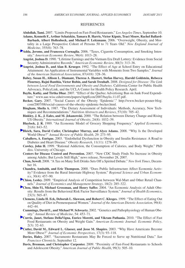
186 AMErICAN ECoNoMIC JourNAL: AppLIEd ECoNoMICS JANuAry 2011
REFERENCES
Abdollah, Tami. 2007. “Limits Proposed on Fast-Food Restaurants.” Los Angeles times, September 10.Adams, Kenneth F., Arthur Schatzkin, Tamara B. Harris, Victor Kipnis, Traci Mouw, Rachel Ballard-
Barbash, Albert Hollenbeck, and Michael F. Leitzmann. 2006. “Overweight, Obesity, and Mor-tality in a Large Prospective Cohort of Persons 50 to 71 Years Old.” New England Journal of Medicine, 355(8): 763–78.
Adda, Jerome, and Francesca Cornaglia. 2006. “Taxes, Cigarette Consumption, and Smoking Inten-sity.” American Economic review, 96(4): 1013–28.
Angrist, Joshua D. 1990. “Lifetime Earnings and the Vietnam Era Draft Lottery: Evidence from Social Security Administrative Records.” American Economic review, 80(3): 313–36.
Angrist, Joshua D., and Alan B. Krueger. 1992. “The Effect of Age at School Entry on Educational Attainment: An Application of Instrumental Variables with Moments from Two Samples.” Journal of the American Statistical Association, 87(418): 328–36.
Babey, Susan H., Allison L. Diamant, Theresa A. Hastert, Stefan Harvey, Harold Goldstein, Rebecca Flournoy, Rajni Banthia, Victor Rubin, and Sarah Treuhaft. 2008. designed for disease: the Link between Local Food Environments and obesity and diabetes. California Center for Public Health Advocacy, PolicyLink, and the UCLA Center for Health Policy Research. April.
Baylis, Kathy, and Tirtha Dhar. 2007. “Effect of the Quebec Advertising Ban on Junk Food Expendi-ture.” www.aae.wisc.edu/events/papers/AppEcon/2007/baylis.11.07.pdf.
Becker, Gary. 2007. “Social Causes of the Obesity ‘Epidemic’.” http://www.becker-posner-blog.com/2007/08/social-causes-of-the-obesity-epidemic-becker.html.
Bingham, Sheila A. 1987. “The Dietary Assessment of Individuals: Methods, Accuracy, New Tech-niques and Recommendations.” Nutrition Abstracts and reviews, 57(10): 705–42.
Binkley, J. K., J. Eales, and M. Jekanowski. 2000. “The Relation between Dietary Change and Rising US Obesity.” International Journal of obesity, 24(8): 1032–39.
Blaylock, J. R. 1989. “An Economic Model of Grocery Shopping Frequency.” Applied Economics, 21(6): 843–52.
Bleich, Sara, David Cutler, Christopher Murray, and Alyce Adams. 2008. “Why Is the Developed World Obese?” Annual review of public Health, 29: 273–95.
Caballero, A. Enrique. 2003. “Endothelial Dysfunction in Obesity and Insulin Resistance: A Road to Diabetes and Heart Disease.” obesity research, 11(11): 1278–89.
Cawley, John H. 1999. “Rational Addiction, the Consumption of Calories, and Body Weight.” PhD diss. University of Chicago.
Centers for Disease Control and Prevention. 2007. “New CDC Study Finds No Increase in Obesity among Adults; But Levels Still High,” news release, November 28, 2007.
Chan, Sewell. 2008. “A Tax on Many Soft Drinks Sets Off a Spirited Debate.” New york times, Decem-ber 16.
Chandra, Amitabh, and Eric Thompson. 2000. “Does Public Infrastructure Affect Economic Activ-ity? Evidence from the Rural Interstate Highway System.” regional Science and urban Econom-ics, 30(4): 457–90.
Chiou, Lesley. 2009. “Empirical Analysis of Competition between Wal-Mart and Other Retail Chan-nels.” Journal of Economics and Management Strategy, 18(2): 285–322.
Chou, Shin-Yi, Michael Grossman, and Henry Saffer. 2004. “An Economic Analysis of Adult Obe-sity: Results from the Behavioral Risk Factor Surveillance System.” Journal of Health Economics, 23(3): 565–87.
Clemens, Linda H. Eck, Deborah L. Slawson, and Robert C. Klesges. 1999. “The Effect of Eating Out on Quality of Diet in Premenopausal Women.” Journal of the American dietetic Association, 99(4): 442–44.
Cummings, David E., and Michael W. Schwartz. 2002. “Genetics and Pathophysiology of Human Obe-sity.” Annual review of Medicine, 54: 453–71.
Currie, Janet, Stefano DellaVigna, Enrico Moretti, and Vikram Pathania. 2010. “The Effect of Fast Food Restaurants on Obesity and Weight Gain.” American Economic Journal: Economic policy, 2(3): 32–63.
Cutler, David M., Edward L. Glaeser, and Jesse M. Shapiro. 2003. “Why Have Americans Become More Obese?” Journal of Economic perspectives, 17(3): 93–118.
Davies, Haley. 2007. “Sacramento Restaurants May Be Forced to Serve up Nutritional Data.” San Francisco Chronicle, September 12.
Davis, Brennan, and Christopher Carpenter. 2009. “Proximity of Fast-Food Restaurants to Schools and Adolescent Obesity.” American Journal of public Health, 99(3): 505–10.
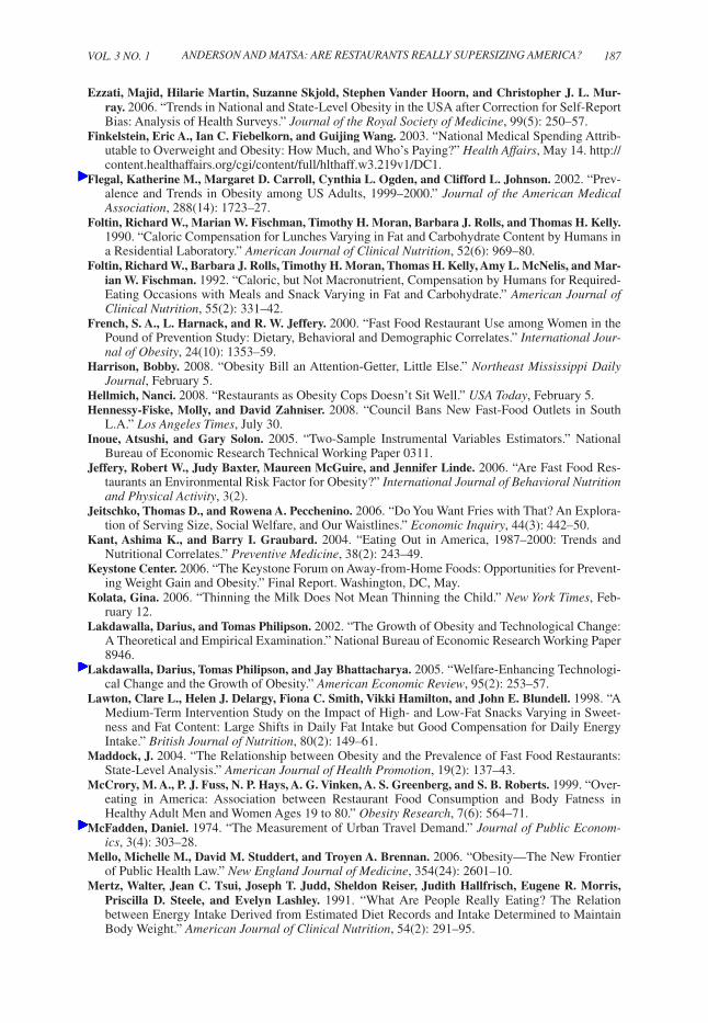
VoL. 3 No. 1 187ANdErSoN ANd MAtSA: ArE rEStAurANtS rEALLy SupErSIzINg AMErICA?
Ezzati, Majid, Hilarie Martin, Suzanne Skjold, Stephen Vander Hoorn, and Christopher J. L. Mur-ray. 2006. “Trends in National and State-Level Obesity in the USA after Correction for Self-Report Bias: Analysis of Health Surveys.” Journal of the royal Society of Medicine, 99(5): 250–57.
Finkelstein, Eric A., Ian C. Fiebelkorn, and Guijing Wang. 2003. “National Medical Spending Attrib-utable to Overweight and Obesity: How Much, and Who’s Paying?” Health Affairs, May 14. http://content.healthaffairs.org/cgi/content/full/hlthaff.w3.219v1/DC1.
Flegal, Katherine M., Margaret D. Carroll, Cynthia L. Ogden, and Clifford L. Johnson. 2002. “Prev-alence and Trends in Obesity among US Adults, 1999–2000.” Journal of the American Medical Association, 288(14): 1723–27.
Foltin, Richard W., Marian W. Fischman, Timothy H. Moran, Barbara J. Rolls, and Thomas H. Kelly. 1990. “Caloric Compensation for Lunches Varying in Fat and Carbohydrate Content by Humans in a Residential Laboratory.” American Journal of Clinical Nutrition, 52(6): 969–80.
Foltin, Richard W., Barbara J. Rolls, Timothy H. Moran, Thomas H. Kelly, Amy L. McNelis, and Mar-ian W. Fischman. 1992. “Caloric, but Not Macronutrient, Compensation by Humans for Required-Eating Occasions with Meals and Snack Varying in Fat and Carbohydrate.” American Journal of Clinical Nutrition, 55(2): 331–42.
French, S. A., L. Harnack, and R. W. Jeffery. 2000. “Fast Food Restaurant Use among Women in the Pound of Prevention Study: Dietary, Behavioral and Demographic Correlates.” International Jour-nal of obesity, 24(10): 1353–59.
Harrison, Bobby. 2008. “Obesity Bill an Attention-Getter, Little Else.” Northeast Mississippi daily Journal, February 5.
Hellmich, Nanci. 2008. “Restaurants as Obesity Cops Doesn’t Sit Well.” uSA today, February 5. Hennessy-Fiske, Molly, and David Zahniser. 2008. “Council Bans New Fast-Food Outlets in South
L.A.” Los Angeles times, July 30.Inoue, Atsushi, and Gary Solon. 2005. “Two-Sample Instrumental Variables Estimators.” National
Bureau of Economic Research Technical Working Paper 0311.Jeffery, Robert W., Judy Baxter, Maureen McGuire, and Jennifer Linde. 2006. “Are Fast Food Res-
taurants an Environmental Risk Factor for Obesity?” International Journal of Behavioral Nutrition and physical Activity, 3(2).
Jeitschko, Thomas D., and Rowena A. Pecchenino. 2006. “Do You Want Fries with That? An Explora-tion of Serving Size, Social Welfare, and Our Waistlines.” Economic Inquiry, 44(3): 442–50.
Kant, Ashima K., and Barry I. Graubard. 2004. “Eating Out in America, 1987–2000: Trends and Nutritional Correlates.” preventive Medicine, 38(2): 243–49.
Keystone Center. 2006. “The Keystone Forum on Away-from-Home Foods: Opportunities for Prevent-ing Weight Gain and Obesity.” Final Report. Washington, DC, May.
Kolata, Gina. 2006. “Thinning the Milk Does Not Mean Thinning the Child.” New york times, Feb-ruary 12.
Lakdawalla, Darius, and Tomas Philipson. 2002. “The Growth of Obesity and Technological Change: A Theoretical and Empirical Examination.” National Bureau of Economic Research Working Paper 8946.
Lakdawalla, Darius, Tomas Philipson, and Jay Bhattacharya. 2005. “Welfare-Enhancing Technologi-cal Change and the Growth of Obesity.” American Economic review, 95(2): 253–57.
Lawton, Clare L., Helen J. Delargy, Fiona C. Smith, Vikki Hamilton, and John E. Blundell. 1998. “A Medium-Term Intervention Study on the Impact of High- and Low-Fat Snacks Varying in Sweet-ness and Fat Content: Large Shifts in Daily Fat Intake but Good Compensation for Daily Energy Intake.” British Journal of Nutrition, 80(2): 149–61.
Maddock, J. 2004. “The Relationship between Obesity and the Prevalence of Fast Food Restaurants: State-Level Analysis.” American Journal of Health promotion, 19(2): 137–43.
McCrory, M. A., P. J. Fuss, N. P. Hays, A. G. Vinken, A. S. Greenberg, and S. B. Roberts. 1999. “Over-eating in America: Association between Restaurant Food Consumption and Body Fatness in Healthy Adult Men and Women Ages 19 to 80.” obesity research, 7(6): 564–71.
McFadden, Daniel. 1974. “The Measurement of Urban Travel Demand.” Journal of public Econom-ics, 3(4): 303–28.
Mello, Michelle M., David M. Studdert, and Troyen A. Brennan. 2006. “Obesity––The New Frontier of Public Health Law.” New England Journal of Medicine, 354(24): 2601–10.
Mertz, Walter, Jean C. Tsui, Joseph T. Judd, Sheldon Reiser, Judith Hallfrisch, Eugene R. Morris, Priscilla D. Steele, and Evelyn Lashley. 1991. “What Are People Really Eating? The Relation between Energy Intake Derived from Estimated Diet Records and Intake Determined to Maintain Body Weight.” American Journal of Clinical Nutrition, 54(2): 291–95.
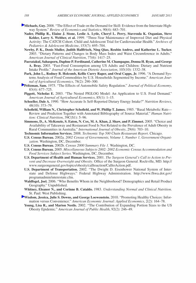
188 AMErICAN ECoNoMIC JourNAL: AppLIEd ECoNoMICS JANuAry 2011
Michaels, Guy. 2008. “The Effect of Trade on the Demand for Skill: Evidence from the Interstate High-way System.” review of Economics and Statistics, 90(4): 683–701.
Nader, Phillip R., Elaine J. Stone, Leslie A. Lytle, Cheryl L. Perry, Stavroula K. Osganian, Steve Kelder, Larry S. Webber, et al. 1999. “Three-Year Maintenance of Improved Diet and Physical Activity: The CATCH Cohort. Child and Adolescent Trial for Cardiovascular Health.” Archives of pediatrics & Adolescent Medicine, 153(7): 695–704.
Newby, P. K., Denis Muller, Judith Hallfrisch, Ning Qiao, Reubin Andres, and Katherine L. Tucker. 2003. “Dietary Patterns and Changes in Body Mass Index and Waist Circumference in Adults.” American Journal of Clinical Nutrition, 77(6): 1417–25.
Paeratakul, Sahasporn, Daphne P. Ferdinand, Catherine M. Champagne, Donna H. Ryan, and George A. Bray. 2003. “Fast-Food Consumption among US Adults and Children: Dietary and Nutrient Intake Profile.” Journal of the American dietetic Association, 103(10): 1332–38.
Park, John L., Rodney B. Holcomb, Kellie Curry Raper, and Oral Capps, Jr. 1996. “A Demand Sys-tems Analysis of Food Commodities by U.S. Households Segmented by Income.” American Jour-nal of Agricultural Economics, 78(2): 290–300.
Peltzman, Sam. 1975. “The Effects of Automobile Safety Regulation.” Journal of political Economy, 83(4): 677–725.
Piggott, Nicholas E. 2003. “The Nested PIGLOG Model: An Application to U.S. Food Demand.” American Journal of Agricultural Economics, 85(1): 1–15.
Schoeller, Dale A. 1990. “How Accurate Is Self-Reported Dietary Energy Intake?” Nutrition reviews, 48(10): 373–79.
Schofield, William N., Christopher Schofield, and W. Phillip T. James. 1985. “Basal Metabolic Rate––Review and Prediction Together with Annotated Bibliography of Source Material.” Human Nutri-tion: Clinical Nutrition, 39C(S1): 5–96.
Simmons, D., A. McKenzie, S. Eaton, N. Cox, M. A. Khan, J. Shaw, and P. Zimmet. 2005. “Choice and Availability of Takeaway and Restaurant Food Is Not Related to the Prevalence of Adult Obesity in Rural Communities in Australia.” International Journal of obesity, 29(6): 703–10.
Technomic Information Services. 2008. technomic top 500 Chain restaurant report. Chicago.U.S. Census Bureau. 2002a. 2002 Census of governments, Volume 1, Number 1, government organi-
zation. Washington, DC, December.U.S. Census Bureau. 2002b. Census 2000 Summary File 1. Washington, DC.U.S. Census Bureau. 2005. Miscellaneous Subjects 2002: 2002 Economic Census Accommodation and
Food Services Subject Series. Washington, DC, December.U.S. Department of Health and Human Services. 2001. the Surgeon general’s Call to Action to pre-
vent and decrease overweight and obesity. Office of the Surgeon General. Rockville, MD. http://www.surgeongeneral.gov/topics/obesity/calltoaction/CalltoAction.pdf.
U.S. Department of Transportation. 2002. “The Dwight D. Eisenhower National System of Inter-state and Defense Highways.” Federal Highway Administration. http://www.fhwa.dot.gov/ programadmin/interestate.cfm.
Waldfogel, Joel. 2006. “Who Benefits Whom in the Neighborhood? Demographics and Retail Product Geography.” Unpublished.
Whitney, Eleanor N., and Corinne B. Cataldo. 1983. understanding Normal and Clinical Nutrition. St. Paul: West Publishing.
Wisdom, Jessica, Julie S. Downs, and George Loewenstein. 2010. “Promoting Healthy Choices: Infor-mation versus Convenience.” American Economic Journal: Applied Economics, 2(2): 164–78.
Young, Lisa R., and Marion Nestle. 2002. “The Contribution of Expanding Portion Sizes to the US Obesity Epidemic.” American Journal of public Health, 92(2): 246–49.


![WELCOME [] · WELCOME GR Brewer Manual. The simple answer, really, is that since 1957, America’s favorite diners, restaurants and cafés have chosen BUNN as ... Scoop fresh ground](https://static.fdocuments.net/doc/165x107/5bc19bea09d3f2840b8cf5de/welcome-welcome-gr-brewer-manual-the-simple-answer-really-is-that-since.jpg)