Are Leveraged and Inverse ETFs the New Portfolio Insurers
43
Finance and Economics Discussion Series Divisions of Research & Statistics and Monetary Affairs Federal Reserve Board, Washington, D.C. Are Leveraged and Inverse ETFs the New Portfolio Insurers? Tugkan Tuzun 2013-48 NOTE: Staff working papers in the Finance and Economics Discussion Series (FEDS) are preliminary mate rial s circulated to stimulate discuss ion and crit ical commen t. The analysis and concl usions set forth are those of the authors and do not indicate concurrence by other members of the research staff or the Board of Governors. References in publications to the Finance and Economics Discussion Series (other than acknowledgement) should be cleared with the author(s) to protect the tentative character of these papers.
-
Upload
wegerg123343 -
Category
Documents
-
view
227 -
download
0
Transcript of Are Leveraged and Inverse ETFs the New Portfolio Insurers
7/27/2019 Are Leveraged and Inverse ETFs the New Portfolio Insurers
http://slidepdf.com/reader/full/are-leveraged-and-inverse-etfs-the-new-portfolio-insurers 1/43
Finance and Economics Discussion SeriesDivisions of Research & Statistics and Monetary Affairs
Federal Reserve Board, Washington, D.C.
Are Leveraged and Inverse ETFs the New Portfolio Insurers?
Tugkan Tuzun
2013-48
NOTE: Staff working papers in the Finance and Economics Discussion Series (FEDS) are preliminarymaterials circulated to stimulate discussion and critical comment. The analysis and conclusions set forthare those of the authors and do not indicate concurrence by other members of the research staff or theBoard of Governors. References in publications to the Finance and Economics Discussion Series (other thanacknowledgement) should be cleared with the author(s) to protect the tentative character of these papers.

7/27/2019 Are Leveraged and Inverse ETFs the New Portfolio Insurers
http://slidepdf.com/reader/full/are-leveraged-and-inverse-etfs-the-new-portfolio-insurers 2/43
Are Leveraged and Inverse ETFs the New PortfolioInsurers?
Tugkan Tuzun∗
Board of Governors of the Federal Reserve System
First Draft: December 18, 2012
This Draft: July 16, 2013
ABSTRACT
This paper studies Leveraged and Inverse Exchange Traded Funds (LETFs)from a financial stability perspective. Mechanical positive-feedback rebalancing of LETFs resembles the portfolio insurance strategies, which contributed to the stockmarket crash of October 19, 1987 (Brady Report, 1988). I show that a 1% increasein broad stock-market indexes induces LETFs to originate rebalancing flows equiv-alent to $1.04 billion worth of stock. Price-insensitive and concentrated tradingof LETFs results in price reaction and extra volatility in underlying stocks. Im-plied price impact calculations and empirical results suggest that they contributedto the stock market volatility in the 2008-2009 financial crisis and in the secondhalf of 2011 when the European sovereign debt crisis came to the forefront. Al-though LETFs are not as large as portfolio insurers of the 1980s and have notbeen proven to disrupt stock market activity, their large and concentrated tradingcould be destabilizing during periods of high volatility.
Keywords: ETFs, Price Impact, Financial Stability, Stock Market Crashes
∗Tugkan Tuzun ([email protected]) is with the Federal Reserve Board. Address: 20th and C St.NW, MS 114, Washington, DC 20551. This paper benefited from discussions with Pete Kyle and hissuggestions. I am grateful to Celso Brunetti, Eric Engstrom, Hayne Leland, Michael Palumbo, SteveSharpe and Jeremy Stein for their useful comments. I also thank the seminar participants at the CFTC,Federal Reserve Board and the Office of Financial Research. All errors are my own. Joost Bottenbleyand Suzanne Chang provided excellent research assistance. The views expressed in this paper are myown and do not represent the views of the Federal Reserve Board, Federal Reserve System or their staff.
1
7/27/2019 Are Leveraged and Inverse ETFs the New Portfolio Insurers
http://slidepdf.com/reader/full/are-leveraged-and-inverse-etfs-the-new-portfolio-insurers 3/43
I. Introduction
The complex structure and behavior of Leveraged and Inverse Exchange Traded Funds
(LETFs) have raised important questions about their implications for financial stability.
LETFs are exchange-traded products that typically promise multiples of daily index
returns. Generating multiples of daily index returns gives rise to two important charac-
teristics of LETFs that are similar to the portfolio insurance strategies that are thought
to have contibuted to the stock market crash of October 19, 1987 (Brady Report, 1988).
(1) LETFs rebalance their portfolios daily by trading in the same direction as the changes
in the underlying index, buying when the index increases and selling when the index
decreases. (2) This rebalancing requirement of LETFs is predictable and may attract
anticipatory trading. Portfolio insurance strategies were commonly used by asset man-
agers in the 1980s and their use reportedly declined after the stock market crash of 1987.
Portfolio insurance is a dynamic trading strategy, which synthetically replicates options
to protect investor portfolios. Synthetic replication of options requires buying in a ris-
ing market and selling in a declining market. Rather than buying and selling stocks as
the market moves, portfolio insurers generally traded index futures. The Brady Report
(1988) suggests that portfolio insurance related selling accounted for a significant frac-
tion of the selling volume on October 19, 1987. The report also notes that “aggressive-
oriented institutions” sold in anticipation of the portfolio insurance trades. This selling,
in turn, stimulated further reactive selling by portfolio insurers. Price-insensitive and
predictable trading of portfolio insurers contributed to the price decline of 29% in S&P
500 futures through a selling “cascade”.
This paper studies the impact of equity LETFs on various stock categories while
emphasizing their implications for financial stability and similarities with portfolio in-
surance strategies. Promising a certain multiple of daily index return induces LETFs to
2

7/27/2019 Are Leveraged and Inverse ETFs the New Portfolio Insurers
http://slidepdf.com/reader/full/are-leveraged-and-inverse-etfs-the-new-portfolio-insurers 4/43
rebalance their portfolios daily to maintain their target stock-to-cash ratios. Rebalanc-
ing demand of a LETF can be derived from a simple formula, which dictates the LETF
to buy when its target index goes up and sell when its target index goes down. Al-
though their rebalancing formulas are more complex, portfolio insurers also trade in the
same direction as the market to maintain their stock-to-cash ratios constant. Anectodal
evidence suggests that LETFs commonly use swaps and futures contracts to rebalance
their portfolios. Swap counterparties of LETFs are likely to hedge their positions in
equity spot or futures markets. If LETFs use index futures, index arbitraguers transfer
the price pressure from the futures market to the stock market. If the LETFs account
for a significant fraction of trading, their rebalancing activity should leave its imprint
on the stock indexes they follow.
The size of LETF rebalancing demand varies with their net assets and the multiples
of daily index return they promise. Based on total net asset value of $20.14 billion as of
December 15, 2011, when broad stock-market indexes change by 1%, LETFs rebalancing
demand totals $1.04 billion worth of stock. This is roughly 0.84% of daily stock-market
volume (excluding the volume of the ETFs and the Depository Receipts) in the United
States. Kyle and Obizhaeva (2012) calculate that the portfolio insurers in 1987 would
sell $4 billion (4% of stock-plus-derivatives volume) in response to a 4% price decline in
the Dow Jones Industrial Average. Although LETFs are not as large as the portfolio
insurers were in 1987, LETF rebalancing in response to a large market move, especially
in periods of high volatility, could still pose risks. For example, the Flash Crash of May6, 2010 was triggered by a $4.1 billion (75,000 contracts of E-Mini S&P 500 Futures)
sell order, which is equivalent to only 3% of the E-Mini S&P 500 Futures daily volume
(CFTC-SEC Report, 2010). With a large market move, such as 4%, the total rebalancing
flows of LETFs would be equivalent to this “Flash Crash” order. Rebalancing in the
last hour of trading could, in fact, reduce the possibility of a significant price dislocation
3
7/27/2019 Are Leveraged and Inverse ETFs the New Portfolio Insurers
http://slidepdf.com/reader/full/are-leveraged-and-inverse-etfs-the-new-portfolio-insurers 5/43
since the market close could serve as a prolonged circuit breaker. On the other hand,
executing orders within a short period of time, such as the last hour of trading, may
cause disproportionate price changes. A significant price dislocation at the market close
may also impair investor confidence. If the market closes with depressed prices, the
stock market could experience large investor outflows overnight.
Naturally, LETFs follow different stock-market indexes and the size of their rebalanc-
ing differs across stock categories. LETF rebalancing is an important fraction of daily
volume, especially in financial and small stocks. For instance, if the Russell 1000 Finan-
cial Services Index increases by 1%, the rebalancing demand of LETFs totals roughly
2% of the daily volume for an average financial stock. Furthermore, academic stud-
ies (Cheng and Madhavan, 2009; Bai et al., 2012) and anectodal reports12 suggest that
LETFs rebalance their portfolio in the last hour of trading. Therefore, a large market
move could make these stocks vulnerable near the market close, or even before to the
extent that opportunistic traders react in anticipation of subsequent LETF rebalancing.
Although LETF activity is relatively small in some stock categories, LETF rebal-
ancing in the last hour of trading leads to price reaction and extra volatility in all stock
categories. For instance, if the S&P 500 index goes up by 1%, LETF rebalancing de-
mand results in a 6.9 basis-point increase in price and a 22.7 basis-point increase in daily
volatility in an average large-cap stock.
The size of the price reaction of LETF Flows inferred from empirical specifications
could be an underestimate if prices at 3:00 pm already reflect to some extent investors an-ticipation of subsequent LETF rebalancing. By directly implementing Kyle and Obizhaeva
(2011a,b) measure of price impact, I show that the implied price impact of LETF re-
balancing on financial markets was notable especially during the financial crisis of 2008-
1Jason Zweig, “Will Leveraged ETFs Put Cracks in Market Close?, Wall Street Journal, April 18,2009
2Andrew Ross Sorkin, “Volatility, Thy Name is E.T.F.”, New York Times, October 10, 2011
4
7/27/2019 Are Leveraged and Inverse ETFs the New Portfolio Insurers
http://slidepdf.com/reader/full/are-leveraged-and-inverse-etfs-the-new-portfolio-insurers 6/43
2009 and at the height of the European sovereign debt crisis. If LETF rebalancing exerts
significant price pressure, this price pressure could amplify the market movements. Al-
though LETFs have not been proven to disrupt stock markets, it is plausible that during
periods of high volatility, their impact in response to a large market move could reach a
tipping point for a“cascade” reaction.
II. Literature Review
In the United States, Exchange Traded Funds (ETFs3
) have grown rapidly and hold
nearly $1.3 trillion in net assets as of September 2012. The growing size of the ETF indus-
try has prompted researchers to analyze recent trends. Agapova (2012) and Huang and Guedj
(2009) suggest that ETFs are close but not perfect substitutes for index mutual funds.
Poterba and Shoven (2002) show that the largest ETF (the SPDR trust) offers simi-
lar pre-tax and after-tax returns as the largest index fund (the Vanguard Index 500).
Buetow and Henderson (2012) argue that, on average, ETFs closely track their target
indexes. Commodity ETFs typically roll contacts in the futures markets as they expire.
Bessembinder et al. (2012) estimate the transaction costs of these ETF “roll” trades in
the crude oil futures market and cannot find compelling evidence for predatory trading.
Another line of literature studies the arbitrage relationship between ETFs and their un-
derlying stocks. Ben-David et al. (2012) argue that ETFs propogate liquidity shocks to
the securities in their baskets. Analyzing the “Flash Crash” of May 6, 2010, Madhavan
(2011) argues that ETFs are vulnerable in market disruptions because pricing of individ-
ual component securities becomes more difficult. Several other academics have studied
the complex return structure of LETFs. Cheng and Madhavan (2009), Jarrow (2010),
Avellanda and Zhang (2009) show that LETF returns could be significantly different
3Includes Exhange Traded Notes (ETN). ETNs are “Uncollateralized Debt Instruments” and in-vestors do not own the investment assets. ETNs are roughly 2% of the ETF industry.
5
7/27/2019 Are Leveraged and Inverse ETFs the New Portfolio Insurers
http://slidepdf.com/reader/full/are-leveraged-and-inverse-etfs-the-new-portfolio-insurers 7/43
than their multiple of target index returns for holding periods longer than one day. The
long-horizon return structure of LETFs that rebalance daily is alone not suitable for the
investment horizons of many investors4.
The daily rebalancing of LETFs has also stimulated academic research. Trainor
(2010) cannot find evidence that suggests Leveraged ETFs increase volatility. Focusing
on the S&P 500 index returns and aggregate LETF rebalancing demands, Cheng and Madhavan
(2009) argue that aggregate LETF rebalancing demand has price pressure on the end-of-
day S&P 500 index returns. Similarly, Bai et al. (2012) examine the impact of 6 LETFs
on 63 real estate sector stocks and find evidence for both end-of-day LETF price pressure
and extra volatility. My study contributes to this literature by quantifying the implied
price effects of LETF rebalancing through examining the impact of all US-listed equity
LETFs on several stock categories.
Several papers studied the role of portfolio insurers in the 1987 stock market crash.
Contrary to the Brady Report (1988), Brennan and Schwartz (1989) suggest that the ef-
fect of portfolio insurance strategies is too small to explain the 1987 crash. Gennotte and Leland
(1990) argue that informational changes, rather than the selling by portfolio insurers,
are needed to explain the 1987 crash. They argue that if mistaken by informed trading,
portfolio insurance strategies could have a much greater price impact-an impact of mag-
nitute similar to what was observed in 1987. With the “Flash Crash” of May 6, 2010,
the focus on market disruptions and large orders has been renewed. CFTC-SEC Report
(2010) concludes that rapid execution of a large sell order triggered the “Flash Crash”
5
.Kyle and Obizhaeva (2012) examine the five stock market crashes, including the 1987
crash, with documented large sells during those events. They show that price declines in
those events are similar in magnitude to price impact of large sales suggested by market
4Appendix explores the drivers of the investor demand for these products.5See Kirilenko et al. (2011) for a detailed examination of different trader behaviors on May 6, 2010
6

7/27/2019 Are Leveraged and Inverse ETFs the New Portfolio Insurers
http://slidepdf.com/reader/full/are-leveraged-and-inverse-etfs-the-new-portfolio-insurers 8/43
microstructure invariance (Kyle and Obizhaeva, 2011a,b). My study extends their work
by computing the price impact estimates of LETFs implied by market microstructure
invariance.
III. LETF Rebalancing
LETFs typically promise a certain multiple of a daily index return. Producing mul-
tiples of daily returns forces LETFs to rebalance their portfolios in response to price
movements. Daily rebalancing ensures that LETFs maintain their stock-to-cash ratios
at market close. The mechanics of LETF rebalancing can be illustrated in a simple asset
allocation setting.6
An asset allocation problem can be written in the following way:
W t = S t + Bt
Asset managers generally invest a certain fraction, δ , of their net assets, W t, into the
risky asset (underlying equity index), S t and the rest,(1-δ ) into the bond market.
W t = δ × W t S t
+ (1 − δ ) × W t Bt
LETFs choose δ consistent with their prospectuses. For example, Leveraged ETFs
have δ =2 or 3 while Inverse ETFs have δ =-1,-2 or -3. Assuming interest rate is zero, if
the underlying index changes by r, then the investment on the index becomes δ (1 + r)W t
and this change is reflected in the size of total portfolio.
6See Cheng and Madhavan (2009) for their derivation of the same rebalancing formula.
7

7/27/2019 Are Leveraged and Inverse ETFs the New Portfolio Insurers
http://slidepdf.com/reader/full/are-leveraged-and-inverse-etfs-the-new-portfolio-insurers 9/43
W t(1 + δ × r) W t+1
= δ (1 + r)W t S ′t
+(1 − δ )W t
Since the LETF is promising δ over the daily return on the index, δ × W t+1 should
be invested on the index to maintain a constant stock-to-cash ratio.
S t+1 = δ × W t+1 = δ × (1 + δ × r) × W t
The rebalancing amount in response to the size of change r in the index can be
calculated as
S t+1 − S ′
t = r × δ × (δ − 1) × W t
It is important to note that when δ ∈ [0,1], the rebalancing amount has the same sign
as r, suggesting that both Inverse and Leveraged ETFs rebalance in the same direction
as their target indexes and their rebalancing do not cancel each other out. Furthermore,
this formula is a function of only the target index change, not its level, making LETF
rebalancing insensitive to the price level.
In practice, LETFs do not have to directly trade in the stock market to rebalance
their portfolios. The use of derivatives, especially futures and swaps, is believed to be
common among LETFs (Cheng and Madhavan, 2009). If they trade futures contracts,
index arbitraguers will transfer this effect from the futures market to the stock market.
If they enter into a swap aggrement, their counterparty is likely to hedge its exposure
and trade in either the futures or the spot market. As a result, regardless of the contracts
LETFs trade, their portfolio rebalancing should leave an imprint on the stock indexes
they target. Brady Report (1988) notes that portfolio insurers commonly used futures
contracts and index arbitraguers propagated these shocks to the stock market, suggesting
8
7/27/2019 Are Leveraged and Inverse ETFs the New Portfolio Insurers
http://slidepdf.com/reader/full/are-leveraged-and-inverse-etfs-the-new-portfolio-insurers 10/43
that the markets for stocks and stock index futures behave as a single integrated market.
More recently, Kirilenko et al. (2011) explain that although the “Flash Crash” of May
6, 2010 was triggered in the futures market, index arbitraguers quickly transmitted this
price shock to the stock market.
IV. Data
Data for this study is collected from multiple sources. LETF information is obtained
from Morningstar Direct, which provides total net assets, net asset value, shares out-
standing and category type for ETFs. After I identify an ETF as a LETF, I check its
prospectus to identify both its target index and the multiple it promises. Only US-listed
equity LETFs promising multiples of daily index returns are included in the sample. I
also use the daily index return series (S&P 500 Index, Russell 1000 Financial Services,
Russell 2000, Russell Mid Cap, Nasdaq 100) from Morningstar Direct. Volume and re-
turn variables for the stocks are calculated from the NYSE Trades and Quotes (TAQ)dataset. Membership history, monthly index weights and float factors are courteously
provided by Russell Indexes for Russell 1000 Financial Services, Russell 2000 and Rus-
sell MidCap Indexes7 . Membership history of S&P500 is obtained from the Center for
Research in Security Prices (CRSP). Membership history of NASDAQ 100 is obtained
from Bloomberg and index weights are calculated with CRSP market capitalization in-
formation. The sample goes from June 19, 2006, when the first equity LETF was offered
in the US, to December 31, 2011.
7Float is the number of shares available for trading and many stock indexes calculate stock weightsfrom float-adjusted market capitalizations.
9

7/27/2019 Are Leveraged and Inverse ETFs the New Portfolio Insurers
http://slidepdf.com/reader/full/are-leveraged-and-inverse-etfs-the-new-portfolio-insurers 11/43
V. LETFs and Target Stock-Market Indexes
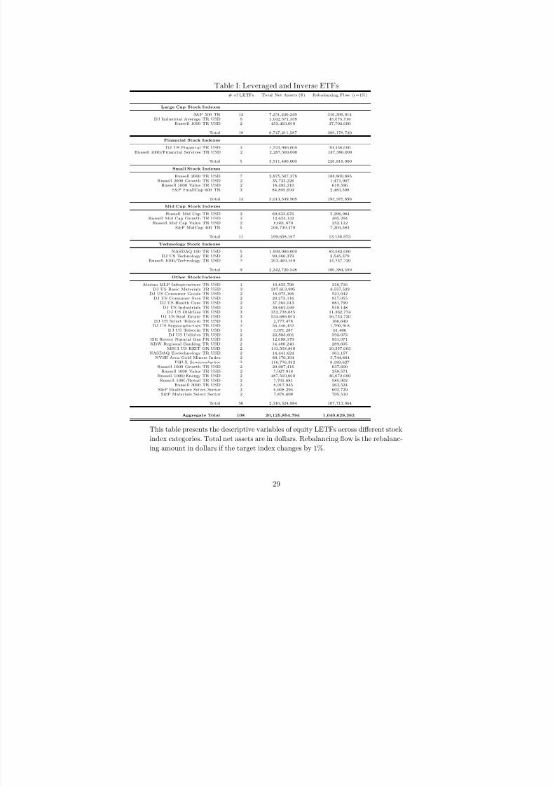
Table I summarizes the distribution of LETFs over stock-market index categories as of
December 15, 2011. Total net assets, number of LETFs, target stock index and LETF
rebalancing flows in response to a 1% change in the target index are reported. The
biggest LETF category is the large stock LETFs and the majority of them follow the
S&P 500. In this category, there are 19 LETFs with $8.7 billion in net assets. A 1%
increase in large stock indexes generates roughly $400 million of rebalancing flow from
these LETFs. The net assets of 5 LETFs, which follow financial stock indexes, total
$3.5 billion and their rebalancing flow is $ 226.8 million in response to a 1% increase in
financial stock indexes. 14 LETFs exist in the small stock category with $3 billion in
net assets. A 1% increase in small stock indexes induces these LETFs to demand $193
million worth of stocks. The mid-cap stock category is the smallest in size with roughly
$ 299 million net assets in total managed by 11 LETFs. Their rebalancing flow is only
$ 13 million when there is a 1% increase in mid cap stock indexes. There are 9 LETFs
with $2.2 billion in net assets following technology stock indexes and their rebalancing
flow totals $ 100 million if technology stock indexes go up by 1%. In total, there are 108
equity LETFs in the US with roughly $ 20 billion in net assets. These LETFs originate
$ 1.04 billion in rebalancing flows if the broad stock-market indexes go up by 1%. Daily
volume of the stock market (excluding ETFs and Depository Receipts) averaged $131
billion in December 2011. Hence, LETF rebalancing flows in response to a 1% increase
in stock prices are equivalent to 0.79% of stock-market volume. Because LETFs also use
swap and futures contracts, LETF rebalancing is less than 0.79% of the total volume
of the stock, futures and swaps markets combined. Although their size appears to be
smaller than portfolio insurers of 1987, it is essential to explore the relative size and
effect of LETF rebalacing in various stock categories.
10

7/27/2019 Are Leveraged and Inverse ETFs the New Portfolio Insurers
http://slidepdf.com/reader/full/are-leveraged-and-inverse-etfs-the-new-portfolio-insurers 12/43
A. LETF Performance and Rebalancing
LETFs are forced to rebalance daily to avoid tracking errors by maintaining constant
stock-to-cash ratios. Low tracking errors can be interpreted as successful portfolio rebal-
ancing. Because LETFs promise certain multiples of daily target index returns, I assess
their performance at daily frequency by using the following regression.
R j,t = α + β (δ j × RIndex j,t ) + ǫ j,t (1)
The S&P 500, Russell 1000 Financial Services, Russell 2000, Russell MidCap and
NASDAQ 100 are used as target indexes for the respective LETF categories defined in
Table I. δ j is the multiple LETF j promises. The variables are winsorized at the 1%
and 99% levels to remove the effect of outliers. The regression is run for each LETF
individually and Table II reports the summary statistics of the regression coefficients
and Adj-R2’s computed within each category. The asset-weighted and equally-weighted
means and medians of α are all close to zero. In absolute value, equally-weighted mean of α range from 0.01 basis points for the large category to 3.2 basis points for the financial
category. Asset-weighted means of α are lower in absolute value and range from 0.01 for
the large category to 1.6 basis points for the small category. Asset-weighted means of
β are close to 1 and range from 0.9 for the technology category to 1.03 for the mid-cap
category. Similarly, asset-weighted means of R2 are quite high. These results suggest
that LETFs, especially the ones with large net assets, rebalance regularly since they are,
on average, successful in delivering multiples of their target indexes at daily frequency.
B. LETF Rebalancing Flows and Underlying Stocks
LETF categories defined in Table I are collapsed into one target stock index in each
category. For simplicity, I assume that the LETFs following large stock indexes aim to
11
7/27/2019 Are Leveraged and Inverse ETFs the New Portfolio Insurers
http://slidepdf.com/reader/full/are-leveraged-and-inverse-etfs-the-new-portfolio-insurers 13/43
target the S&P 500. The Russell 1000 Financial Services and NASDAQ 100 indexes are
chosen for financial and technology categories. Small and mid-cap LETFs are assumed
to follow the Russell 2000 and Russell Mid-Cap Stock Indexes, respectively.
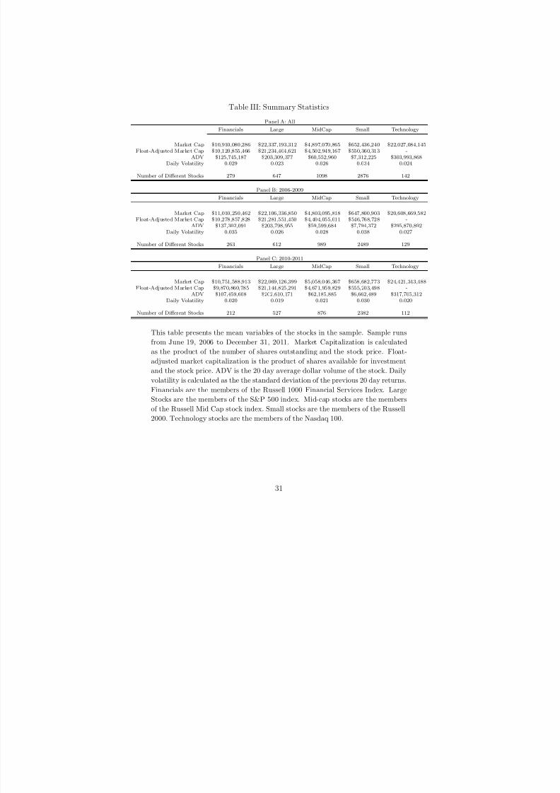
Panel A of Table III reports the summary statistics for various stock categories from
June 2006 to December 2011. The financial category includes the members of the Russell
1000 Financial Services Index. Float-adjusted and unadjusted market capitalizations of
an average financial stock are $10.1 and $ 10.9 billion, respectively. Daily volatility- the
standard deviation of the previous 20 days’ returns- of an average financial stock is 2.9%.
There are 279 different stocks in this category with $125 million in average daily volume.
The large stock category, which consists of the members of the S&P 500 index, has $21.3
and $22.3 billion in float-unadjusted and -adjusted market capitalizations, respectively.
There are 647 different stocks in the large stock category with an average daily volatility
of 2.3% and volume of $203 million. Going from the mid-cap stock category (Russell
Mid-Cap) to small stock category (Russell 2000), market capitalizations and daily vol-
ume decrease. The daily volume of an average mid-cap stock and small stock are $ 60
million and $7 million, respectively. For an average small stock, float-adjusted market
capitalization, $ 550.3 milion, is considerably different then unadjusted market capital-
ization, $ 652.4 million. Technology stocks, which are the members of the NASDAQ 100
index, have $ 22 billion in average market capitalization, roughly equal to that of large
stocks8. Yet, the daily volume of an average technology stock ($303 million) is higher,
suggesting that they are traded more actively. Panel B and Panel C of Table III reportthe same variables for 2006-2009 and 2010-2011 periods. Higher volatility in all stock
categories, especially among financials, is notable in the earlier sample period due to the
2008-2009 financial crisis. Daily volatility of an average financial stock is 3.5% during
8 Stock-weights for NASDAQ 100 are computed from float-unadjusted market capitalizations sincefloat variable could not be obtained.
12

7/27/2019 Are Leveraged and Inverse ETFs the New Portfolio Insurers
http://slidepdf.com/reader/full/are-leveraged-and-inverse-etfs-the-new-portfolio-insurers 14/43
2006-2009 period and 2.0% during 2010-2011 period. Other stock categories have 70 to
80 basis points higher daily volatility in the earlier sample period.
B.1. Size of Hypothetical LETF Rebalancing Flows
Figure 1 presents the share of total hypothetical rebalancing flows of LETFs for an
average stock as a fraction of its daily volume for each category. Aggregate hypothetical
LETF flows are calculated as the sum of all LETF flows in that category in response
to a 1% increase in the target index and allocated to stocks based on their weights
in the target index. For each stock, its share of hypothetical LETF rebalancing flows
is scaled by its average daily volume. Hypothetical LETF rebalancing flows start in
June 2009, when the first equity LETF was introduced in the US. These flows are
less than 1% of daily volume for an average stock in large, mid-cap and technology
categories. Hypothetical LETF rebalacing flows are considerable for an average stock
in financial and small stock categories. In the beginning of 2009, hypothetical LETF
rebalancing flows become larger than 1% of daily volume in an average financial stock
and fluctuate around 2% of daily volume starting in mid 2009. Hypothetical LETF
rebalancing flows become larger than 2% of daily volume in an average small stock in
2009 and reaches levels as high as 6% of daily volume in 2011. Many studies, such as
Cheng and Madhavan (2009); Bai et al. (2012), and news articles mention that LETFs
carry out their rebalancing in the last hour of trading. Figure 2 shows the aggregate
hypothetical rebalancing flows of LETFs as a fraction of volume in the last hour of trading. These flows are 2-3% of volume in the last hour for average stocks in large,
mid-cap and technology categories. For an average small stock, these flows can be as
large as 18% of volume in the closing hour. Similarly, the ratio of hypothetical LETF
flows to the last hour’s volume is significant for an average financial stock. Hypothetical
LETF rebalancing flows for an average financial stock fluctuate between 4 and 8% after
13
7/27/2019 Are Leveraged and Inverse ETFs the New Portfolio Insurers
http://slidepdf.com/reader/full/are-leveraged-and-inverse-etfs-the-new-portfolio-insurers 15/43
2008 and are equivalent to roughly 6% of volume in the last hour in December 2011.
C. End-of-Day Price Effects of LETF Flows
C.1. Price Reaction of Underlying Stocks
To identify pressure points across stock categories, it is crucial to understand the impact
of LETF rebalancing flows on underlying stocks. LETF rebalancing could result in end-
of-day price reaction and extra volatility in those stocks. Other market participants could
trade in anticipation of LETF flows, making it impossible to estimate the isolated priceimpact of LETF flows. However, the end-of-day net price reaction to LETF rebalancing
and anticipatory trades can be estimated.
To estimate the net price reaction to LETF flows, I implement the regression speci-
fication of Obizhaeva (2009) and allow for control variables.
∆log(P i,c)
σi
= β 0 + β 1 ×LETF Flowi
ADV i+ β 2
∆log(P (i,15:00))
σi
+ ǫi (2)
The left hand side of the regression is constructed as a ratio of two variables.
∆log(P i, c) is the return on a stock i between 15:00pm(ET) and 16:00pm (ET) and
σi is the daily volatility. Explanatory variables are also contructed as ratios of two vari-
ables. LETF Flowi, is the share of stock i from the estimated total LETF rebalancing
flow-calculated as a function of the target index return between the previous day’s close
and 15:00pm-implied by its index weight9
. LETF Flowi is scaled by ADV i, which is thepast 20-day average dollar volume of stock i. The variables used in this regression are
winsorized at the 1% and 99% levels to remove the effect of outliers. Panel A of Table
IV reports the results of the regression for different categories from 2006 to 2011. The
9Intraday target index returns are calculated from the intraday returns of their constituents. Un-reported results verify that close-to-close return of target indexes are statistically equal to the dailyreturns of those indexes obtained from the Morningstar Direct.
14
7/27/2019 Are Leveraged and Inverse ETFs the New Portfolio Insurers
http://slidepdf.com/reader/full/are-leveraged-and-inverse-etfs-the-new-portfolio-insurers 16/43
standard errors are clustered daily. For all categories, the coefficients on LETF flows are
positive and statistically significant, ranging from 0.83 for small stocks to 4.16 for mid
cap stocks. The coefficient estimates and regression R2’s are little changed when the
stock return between the previous day’s close and 15:00pm,∆log(P (i,15:00) )
σ, is controlled.
Regression R2’s in this specification range from 0.76% for the technology category to
6.33% for the financial category. Panel B of Table IV reports the results of the regres-
sion for two subperiods, 2006-2009 and 2010-2011. The coefficients on LETF Flows and
R2’s are higher for most of the categories in the earlier sample period. The coefficients
on LETF Flows go from 0.78 for small stocks to 4.85 for mid-cap stocks for 2006-2009
and they go from 0.88 for small stocks to 2.74 for financial stocks in the post-financial
crisis period.
The coefficients on LETF Flows can be interpreted as a change in price as a percent of
daily volatility in response to LETF flows equivalent to 1% of the volume. For example,
LETF flows equivalent to 1% of stock volume, increases the price of a financial stock by
3.09% of its daily volatility. As of December 2011, when the financial indexes increase by
1%, the share of LETF rebalancing flows is equivalent to 2.1% of volume in an average
financial stock with 2% daily volatility. If the financial stock indexes increase by 1%,
price reaction of an average financial stock in response to LETF rebalancing is 13 basis
points (3.09 × 2.1% × 2%). With the LETF flows in response to a 1% change in the
target indexes and the volatility of average stocks in December 2011, the same calculation
can be done for other categories. The end-of-day price reaction is 6.9 basis points (4.32×0.8% × 2%) in an average large stock, 5.5 basis points (4.28× 0.6% × 2%) in an average
mid cap stock, 12.7 basis points (0.86× 5% × 2.9%) in an average small stock and
6.3 basis points (3.83 ×0.75% × 2.2%) in an average technology stock. Although the
largest price reactions to LETF flows occur in financial and small stock categories, all
other categories show price reactions to LETF portfolio rebalancing, suggesting that
15

7/27/2019 Are Leveraged and Inverse ETFs the New Portfolio Insurers
http://slidepdf.com/reader/full/are-leveraged-and-inverse-etfs-the-new-portfolio-insurers 17/43
LETFs and anticipatory traders in the same direction are stronger than the traders on
the opposite side. Without the traders taking the other side of the LETF rebalancing
activity, the end-of-day effect of the LETF rebalancing could be destabilizing.
Rebalancing in the last hour could also amplify the effect of LETFs since executing
orders within a short period of time may move the prices disproportionately. In contrast,
rebalancing in the last hour has the advantage of limiting the possibility of a price
dislocation because the market close may serve as a prolonged circuit breaker. Yet, if
there are enough traders following the LETF rebalancing, they may start trading well
before the market close and produce similar consequences.
Table V reports the results of the same regression for Market Ups (Positive LETF
Flows) and Market Downs (Negative LETF Flows) seperately. The standard errors are
clustered daily. Coefficients of positive LETF flows range from 0.63 for small stocks to
4.66 for technology stocks and coefficients of negative LETF flows range from 0.80 for
small stocks to 3.60 for large stocks. The coefficient on the LETF Flows in Market Ups
are higher than Market Downs for all but small stocks, indicating that market response
to positive LETF flows is slightly stronger. One explanation for this could be the short-
sale constraints. Market participants who trade in anticipation of LETF flows could be
constrained by short-selling and cannot implement their strategy in Market Downs as
well as in Market Ups.
C.2. Price Reversals
In resilient markets, prices revert back after an order is executed especially if the order
does not carry information about the fundamental value. The resilence of the market
could counteract the late-day price reaction of the LETF rebalancing flows and other
anticipatory trades. I implement the following regression to test if prices revert back the
next day after the portfolio rebalancing of LETFs.
16
7/27/2019 Are Leveraged and Inverse ETFs the New Portfolio Insurers
http://slidepdf.com/reader/full/are-leveraged-and-inverse-etfs-the-new-portfolio-insurers 18/43
∆log(P i,15:00)σi
= β 0 + β 1 ×LETF Flowi
ADV i
t−1
+ β 2∆log(P i)
σi
t−1
+ ǫi (3)
The next day’s return of stock is defined as the return from today’s market close to
15:00 next day, scaled by its daily volaility. Explanatory variables are LETF rebalancing
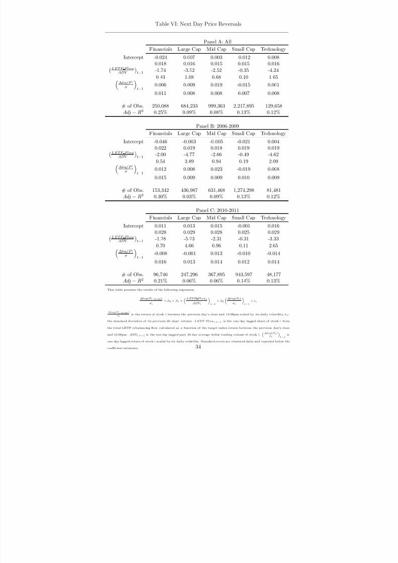
flows and the previous day’s returns. Panel A of Table VI reports the results of this
regression for the full sample period. The standard errors are clustered daily. The
coefficients on LETF Flow are negative and significant for all stock categories, rangingfrom -0.35 for small stocks to -4.24 for technology stocks. Compared with the results
from Table IV, these coefficients are similar in magnitude, suggesting that prices revert
back the next day after LETF rebalancing. Panel B and Panel C of Table VI present
the results of the regression for 2006-2009 and 2010-2011 seperately. The coefficients for
LETF rebalancing flows are negative for all categories in both sample periods. They
range from -0.49 for small stocks to -4.77 for large stocks in the earlier period and go
from -0.31 for small stocks to -5.23 for large stocks in the later period.
C.3. End-of-Day Volatility and LETF Rebalancing
LETF rebalancing and trades in anticipation of LETF rebalancing may affect the stock
volatility in the last hour of trading. To estimate the volatility effects of LETF rebal-
ancing, I use the following regression specification.
∆log(P i,c)
σi
2
= β 0 + β 1 ×
LETF Flowi
ADV i
+ β 2
∆log(P i,(15:00))
σi
2
+ ǫi (4)
The left hand side,
∆log(P i,c)
σi
2
, is the square of the return at the close scaled by daily
return variance.LETF Flowi
ADV i
is the absolute value of LETF Flows scaled by the average
17

7/27/2019 Are Leveraged and Inverse ETFs the New Portfolio Insurers
http://slidepdf.com/reader/full/are-leveraged-and-inverse-etfs-the-new-portfolio-insurers 19/43
daily volume and
∆log(P i,(16:00−15:00) )
σ
2
is the square of daily return until 15:00pm scaled by
daily return variance. The variables used in this regression are winsorized at the 1% and
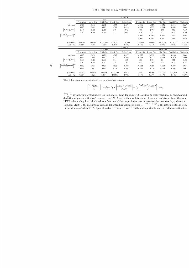
99% levels to remove the effect of outliers. Panel A of Table VII reports the results of this
regression for the entire sample period. The standard errors are clustered daily. When
introduced into the regression,
∆log(P i,(16:00−15:00) )
σ
2
has a positive coefficient and increases
the adjusted R2 for all categories, indicating that high intraday volatility persists through
end-of-day. The LETF Flow variable is positive and significant in all stock categories
and ranges from 0.59 for small stocks to 2.57 for technology stocks. The coefficient on
the LETF Flow variable can be interpreted as the change in return variance as a percent
of daily variance in response to LETF Flows equivalent to 1% of volume. For example,
LETF Flows of 1% of the daily volume increases the return variance, (∆log(P i,c))2, by
1.30 % of the return variance, σ2, in a financial stock. Point estimates can be computed
for average stocks in each category with December 2011 volume and volatility averages.
The end-of-day extra return volatility in response to 1% change in stock indexes is
31.1 basis points ( (1.3 × 2.1% × 2%) in an average financial stock, 22.7 basis points
(
(1.72 × 0.8% × 2%)in an average large stock, 23 basis points (
(1.96 × 0.8% × 2%)
in an average mid-cap stock, 50.5 basis points (
(0.59 × 5% × 2.9%) in an average
small stock and 30.73 basis points (
(0.6 × 0.75% × 2.2%)) in an average technology
stock. These results suggest that LETF rebalancing and possible anticipatory trades of
other market participants account for extra end-of-day volatility for all stock categories.
Panel B of VII reports the results for two sample periods, 2006-2009 and 2010-2011. The
coefficient on the LETF Flow is positive and significant for all categories in both sample
periods. It ranges from 0.64 for small stocks to 5.35 for technology stocks for 2006-2009.
In the post-crisis period, the coefficient is smaller and goes from 0.71 for small stocks to
1.34 for mid-cap stocks.
18

7/27/2019 Are Leveraged and Inverse ETFs the New Portfolio Insurers
http://slidepdf.com/reader/full/are-leveraged-and-inverse-etfs-the-new-portfolio-insurers 20/43
C.4. Intraday Lead-Lag Relations: A Robustness Check
Lo and Mackinlay (1990) document lead-lag patterns in stocks returns. More specifi-
cally, they show that large stock returns lead small stock returns. To control for pos-
sible intraday lead-lag patterns accross and within stock categories, the S&P 500 index
and underlying index returns are included in the end-of-day price reaction and volatility
regressions. As mentioned previously, the underlying index is the Russell 1000 Finan-
cial Services Index for financial stocks, the S&P 500 index for large stocks, the Russell
MidCap Index for midcap stocks, the Russell 2000 for small stocks and the Nasdaq 100
for technology stocks.10 Panel A of Table VIII reports the results for end-of-day price
reaction. The coefficient for the LETF flow is only slighly lower than the previous re-
gressions in Table IV and it continues to be positive and statistically significant for all
stock categories. The coefficient ranges from 0.545 for the small stock category to 3.9 for
the midcap stock category. Panel B of Table VIII reports the results of the regression
of end-of-day volatility. As in Table VII, the coefficient for the absolute value of LETF
Flow continues to be positive and significant after controlling for the intraday volatility
of the underlying index and S&P 500 index returns. These results suggest that the effect
of LETF rebalancing on the end-of-day price and volatility is not driven by the intra-day
lead-lag relationship between small and large stocks.
VI. LETFs and Integrated Markets
The size of the price reaction of LETF Flows inferred from empirical specifications could
be an underestimate if prices at 3:00 pm already reflect to some extent investors anticipa-
tion of subsequent LETF rebalancing. A more direct way to quantify the price impact
10Because the S&P 500 index is the underlying index returns for large stock, the S&P 500 indexreturns are included in the regressions for large stocks only once.
19

7/27/2019 Are Leveraged and Inverse ETFs the New Portfolio Insurers
http://slidepdf.com/reader/full/are-leveraged-and-inverse-etfs-the-new-portfolio-insurers 21/43
of LETF rebalancing flows is to implement the implied price impact measure devel-
oped and calibrated by Kyle and Obizhaeva (2011b,a). Kyle and Obizhaeva (2012) use
this measure to estimate the size of five crash events implied by market microstructure
invariance and conclude that estimates are close to the observed price declines.
Aggregate stock-market segments rather than individual stocks may provide more
accurate price impact estimates if the markets for individual stocks are integrated. In-
tegration of markets may result from various factors. For instance, arbitraguers operate
in multiple markets and exploit arbitrage opportunities by taking opposite positions in
these markets. Hence, they transmit shocks from one market to another. As a result,
market integration leads to faster and more effective transmission of shocks. Moreover,
price shocks to individual stocks can be transmitted to other stocks through leveraged
investor portfolios. Initial losses could lead to margin calls whereby speculators are
forced to deleverage by selling assets in their portfolios, hence leading broader asset
price declines (Brunnermeier and Pedersen, 2009).
The expected price impact of LETF rebalancing flows in a stock-market index with
daily dollar trading volume, ADV, and daily volatility, σ, is given by
∆log(P ) = λ/104.
ADV
40 × 106
1/3
. σ
0.02
4/3
.
LETF Flow
0.01 × ADV
(5)
Kyle and Obizhaeva (2011a) estimate their price impact formula in portfolio transi-
tions data and find λ equal to 5.78. This formula is implemented for 5 different stock-
market indexes; Large, Mid-Cap, Small, Financial and Technology Stock indexes. As
in the previous sections, I use S&P 500 firms for the large category, Russell 2000 firms
for the small category, Russell Mid Cap firms for the mid-cap category, Russell 1000
Financial Services Index firms for the financial category and NASDAQ 100 index stocks
for the technology category. ADV is calculated as the total daily volume of member
20

7/27/2019 Are Leveraged and Inverse ETFs the New Portfolio Insurers
http://slidepdf.com/reader/full/are-leveraged-and-inverse-etfs-the-new-portfolio-insurers 22/43
stocks averaged over the previous 20 days. Volatility is estimated as the standard devi-
ation of the daily index returns in the past 20 days. Finally, LETF Flow is the dollar
amount of LETF rebalancing in response to a 1% change in the target stock-market
index. Measuring the LETF Flows in response to a constant change in the target index
(such as 1%) allows for historical comparison of the impact of LETF rebalancing and
critical assessment for their current size.
Table IX reports the averages of the variables used, and the implied price impact
estimates for 5 stock-market indexes from 2007 to 2011. In 2008 and 2009, volatility is
higher for each category due to the financial crisis. Not suprisingly, the financial stock
index experiences the highest daily volatility, 3.7% in 2008 and 3.4% in 2009. The growth
in net assets of financial LETFs increases the scaled LETF rebalancing flow from 0.4%
in 2008 to 1.02% in 2009. Higher volatility and the growth in financial LETFs leads to
an average implied price impact of 0.97 % in 2009.
If total LETF rebalancing leads to a price impact equal to or greater than the change
in the target index level, it could significantly amplify the target index moves and force
LETFs to carry out further rebalancing. As a result, the implied price impact of 1%
can be considered a critical level for this analysis. Figure 3 plots the implied price
impact of LETF rebalancing in response to a 1% change in the target stock index for
five categories from June 19, 2006 to December 31, 2011. The implied price impact
for the financial category goes above the 1% level in the summer of 2008 and reaches
a level of 1.5% due to over 5% daily volatility after the collapse of Lehman Brothers.The implied price impacts for large, small and technology stock categories also rise and
approach to the 1% level in late 2008. Markets reacted negatively to events following
the Financial Stability Plan announcement on Feb 10, 2009 and the S&P 500 reached a
record low level on March 9, 2009. The implied price impacts for the financial category
skyrockets and almost reaches to the 2.5% level in the first half of 2009 because of over
21

7/27/2019 Are Leveraged and Inverse ETFs the New Portfolio Insurers
http://slidepdf.com/reader/full/are-leveraged-and-inverse-etfs-the-new-portfolio-insurers 23/43
5% daily volatility and the growth in financial LETFs. After the first half of 2009, all
implied price impacts of LETFs remain below the 1% level until August 2011 when
the daily volatility for the financial category increases to 4% due to the concerns about
European soveriegn debt11. The implied price impact estimates for the small and the
financial categories stay above the 1% level through late August and early September
2011.
Kyle and Obizhaeva (2012) compute the implied price impact of portfolio insurers
in October 1987 and find that it ranges from 11.13% to 15.75% over the four days
surrounding the stock-market crash of October 19. Although the implied price impact
estimates of LETFs are not as high as that of portfolio insurers of the 1980s, the implied
price impact of LETFs becomes substantial when daily volatility surges.
Implied price impact results indicate that the imprint of LETF rebalancing left on
the financial stock index should be visible during the 2008-2009 financial crisis and again
in 2011 when the European sovereign debt crisis came to the forefront. Figure 4 plots
the frequency of a 1% price move of the financial stock index in the last hour of trading
given that the index has already moved 1% in the same direction by 3:00pm. This
frequency is calculated from a month’s trading days in which the financial stock index
moved by 1% by 3:00pm 12. The frequency of a large price move in the last hour of
trading is zero until 2007 when the first financial LETF is launched. Consistent with
the implied price impact results, the frequency of a large price move is elevated when
the price volatility is high, reaching 0.8 in the 2008-2009 financial crisis and 0.6 in thesecond half of 2011. These results, combined with the implied price impact estimates,
suggest that LETF rebalancing contributed to the stock market volatility in the 2008-
2009 financial crisis and in the second half of 2011. Although LETF rebalancing has not
11To calm the markets, G7 and ECB held an emergengy meeting on August 8, 2011 after S&Pdowngraded the long-term credit rating of US.
12Although Russell 1000 Financial Services Index was launched in 1996, my sample starts in 2003.
22
7/27/2019 Are Leveraged and Inverse ETFs the New Portfolio Insurers
http://slidepdf.com/reader/full/are-leveraged-and-inverse-etfs-the-new-portfolio-insurers 24/43
been proven to disrupt stock market activity, their large and concentrated trading could
pose risks. The rebalancing of LETFs in the last hour could amplify their impact since
executing orders within a short period of time may move prices disproportionately and
trigger a “cascade” reaction. In contrast, rebalancing in the last hour has the advantage
of limiting the possibility of a price dislocation because the market close may serve as
a prolonged circuit breaker. However, if there are enough traders following the LETF
rebalancing, they may start trading well before the market close and produce similar
consequences.
VII. Conclusion
Contrary to plain vanilla ETFs, LETFs typically rebalance their portfolios daily to main-
tain their stock-to-cash ratios. Maintaining constant stock-to-cash ratios forces LETFs
to rebalance in the same direction as target index moves, selling in a declining market
and buying in a rising market. Similar to portfolio insurance strategies, mechanicalrebalancing of LETFs is predictable and could attract opportunistic traders, who may
originate orders in anticipation of LETF flows. Although the LETFs are not as large
as portfolio insurance strategies of the 1980s in terms of size and impact, daily LETF
rebalancing leaves its imprint on all stock categories.
The implied price impact estimates of LETFs on broad stock-market indexes become
significant during periods of high volatility, especially for the stocks of financial firms.
LETF rebalancing in response to a large market move could amplify the move and
force them to further rebalance which may trigger a “cascade” reaction. Rebalancing
in the last hour of trading could, in fact, reduce the possibility of a price dislocation
since the market close could serve as a prolonged circuit breaker. On the other hand,
executing orders within a short period of time, such as the last hour of trading, may
23

7/27/2019 Are Leveraged and Inverse ETFs the New Portfolio Insurers
http://slidepdf.com/reader/full/are-leveraged-and-inverse-etfs-the-new-portfolio-insurers 25/43
cause disproportionate price changes. A significant price reduction at market close may
also impair investor confidence. If the market closes with depressed prices, the stock
market could experience large investor outflows overnight.
Although the long-horizon return structure of LETFs that rebalance daily is alone
not suitable for the investment horizons of many investors, LETFs delivering multiples of
daily index returns are greater in size and number than the ones delivering multiples of
monthly and quarterly index returns13. Further research is needed to better understand
the drivers of the demand for LETFs delivering multiples of daily index returns.
13There are 7 LETFs which target to deliver multiples of monthly index returns and their total sizeis $ 184.1 million.
24

7/27/2019 Are Leveraged and Inverse ETFs the New Portfolio Insurers
http://slidepdf.com/reader/full/are-leveraged-and-inverse-etfs-the-new-portfolio-insurers 26/43
References
Agapova, A. (2012). Conventional mutual index funds versus exchange traded funds.
Journal of Financial Markets , 14(2):323–343.
Avellanda, M. and Zhang, S. J. (2009). Path-dependence of leveraged etf returns. Work-
ing Paper .
Bai, Q., Bond, S. A., and Hatch, B. (2012). The impact of leveraged and inverse etfs onunderlying stock returns. University of Cincinnati Working Paper .
Ben-David, I., Franzoni, F. A., and Moussawi, R. (2012). Etfs, arbitrage, and shockpropagation. Working Paper .
Bessembinder, H., Carrion, A., Venkataraman, K., and Tuttle, L. A. (2012). Predatoryor sunshine trading? evidence from crude oil etf rolls. Working Paper .
Brady Report (1988). Report of the presidential task force on market mechanisms.
Brennan, M. J. and Schwartz, E. S. (1989). Portfolio insurance and financial marketequilibrium. The Journal of Business , 62(4):455–472.
Brunnermeier, M. K. and Pedersen, L. H. (2009). Market liquidity and funding liquidity.The Review of Financial Studies , 22(6):2201–2238.
Buetow, G. and Henderson, B. (2012). An empirical analysis of exchange traded funds.
Journal of Portfolio Management .
CFTC-SEC Report (2010). Findings regarding the market events of may 6, 2010.
Cheng, M. and Madhavan, A. (2009). Dynamics of leveraged and inverse exchange-traded funds. Journal of Investment Management .
Gennotte, G. and Leland, H. (1990). Market liquidity, hedging, and crashes. The
American Economic Review , 80(5):999–1021.
Hill, J. and Teller, S. (2010). Hedging with inverse etfs. Journal of Indexes .
Huang, J. C. and Guedj, I. (2009). Are etfs replacing index mutual funds? Working Paper .
Jarrow, R. A. (2010). Understanding the risk of leveraged etfs. Finance Research Letters ,7:135–139.
Kirilenko, A., Kyle, A. S., Samadi, M., and Tuzun, T. (2011). The flash crash: Theimpact of high frequency trading on an electronic market. Working Paper .
25

7/27/2019 Are Leveraged and Inverse ETFs the New Portfolio Insurers
http://slidepdf.com/reader/full/are-leveraged-and-inverse-etfs-the-new-portfolio-insurers 27/43
Kyle, A. S. and Obizhaeva, A. (2011a). Market microstructure invariants: Empiricalevidence from portfolio transitions. University of Maryland Working Paper .
Kyle, A. S. and Obizhaeva, A. (2011b). Market microstructure invariants: Theory andimplications of calibration. University of Maryland Working Paper .
Kyle, A. S. and Obizhaeva, A. (2012). Large bets and stock market crashes. University
of Maryland Working Paper .
Lo, A. W. and Mackinlay, A. C. (1990). When are contrarian profits due to stock marketunderreaction? The Review of Financial Studies , 3(2):175–205.
Madhavan, A. (2011). Exchange-traded funds, market structure and the flash crash.Working Paper .
Obizhaeva, A. (2009). Portfolio transitions and stock price dynamics. University of
Maryland Working Paper .
Poterba, J. M. and Shoven, J. B. (2002). Exchange traded funds: A new investmentoption for taxable investors. MIT Department of Economics Working Paper .
Trainor, W. J. (2010). Do leveraged etfs increase volatility? Technology and Investment .
26
7/27/2019 Are Leveraged and Inverse ETFs the New Portfolio Insurers
http://slidepdf.com/reader/full/are-leveraged-and-inverse-etfs-the-new-portfolio-insurers 28/43
Appendix: Investor Flows into LETFs
Since the inception of the first LETF on June 19, 2006, equity LETFs have gainedpopularity among investors and currently have $20B in net assets in the US. Becausethe size and growth of LETFs could be important from a financial stability point of view, examining the drivers of the LETF inflows could explain the intent of their use.There are several hypotheses which explain the purpose of investing in LETFs. Oneexplanation is that LETFs provide an easy access to leverage and short-selling. LETFscan be used by retail investors to easily short stocks or build leverage. Yet, this hypoth-esis cannot explain why LETFs are promising a certain multiple of daily stock indexreturns. Generating a multiple of daily index return requires LETFs to sell when themarket is down and buy when the market is up, resulting in transaction costs. Several
studies (Jarrow (2010); Cheng and Madhavan (2009); Huang and Guedj (2009)) showthat returns of LETFs could be significantly different that their multiple of target indexreturns for holding periods longer than one day. The investment horizon of a retailtrader is typically longer than a day, suggesting that LETFs may not be suitable formany retail investors. Although there are 7 LETFs which target to deliver multiples of monthly index returns, their total size is very small ($ 184.1 million).
Another explanation is that LETFs are used for hedging or portfolio insurance pur-poses. By adding a LETF into his portfolio, an investor may aim to reduce his overallrisk exposure. Hill and Teller (2010) explain that Inverse ETFs could be used by in-vestors for hedging purposes. Hedging a position involves rebalancing the hedge amount
to maintain the desired risk exposure. To explore the hedging hypothesis for LETF usageamong investors, I examine the drivers of investor inflows into the LETFs. The dollaramount of investor flow is calculated as the daily change in LETF shares outstandingmultiplied by its net asset value. The variable of interest, Investor Flow, is defined as thedollar amount of investor flow into an LETF scaled by lagged total net assets. Explana-tory variables considered for this variable are daily lagged Investor Flows, daily laggedLETF returns and daily changes in VIX. Lagged LETF returns are included to explorethe dynamic hedging hypothesis. If an investor is using a LETF for hedging purposes,he dynamically adjusts his hedge position, by selling his shares when his LETF positiongrows and by buying new shares when his LETF position shrinks. As a result, investorsshould redeem their shares when LETFs are generating positive returns and buy newshares when LETFs are giving negative returns. Yet, there are other explanations suchas the disposition effect for negative feedback investments. The disposition effect is thetendency of investors to sell assets whose prices have appreciated while keeping assetswhose prices have declined.
Table X reports the results of the regression for Investor Flows.14 The standarderrors are adjusted for heteroskedasticity. When only the lagged Investor Flows are usedas explanatory variables, Adj − R2 is 3.23%. The coefficients on lagged Investor Flows
14The results are robust to calculating the investor flows as [Net Assets - (1+r) Lagged Net Assets]
27

7/27/2019 Are Leveraged and Inverse ETFs the New Portfolio Insurers
http://slidepdf.com/reader/full/are-leveraged-and-inverse-etfs-the-new-portfolio-insurers 29/43
range from 0.10 to 0.004 and all but one are statistically significant. When the laggedLETF returns are added, Adj − R2 increases to 4.66%. The coefficients on the laggedLETF returns are negative, statistically and economically significant. For instance, if aLETF delivers a 1% return, it experiences outflows equivalent to 0.07% (0.07 × 1%) of its net assets the next day and 0.04% of its net assets on the following day. When thelagged changes of VIX are introduced in the regression, Adj − R2 increases slightly andbecomes 4.72%.
The disposition effect implies that LETFs should have outflows when they deliverpositive returns. Hence, outflows should be more sensitive to recent returns than in-flows. Table X includes the regression results for Inflows and Outflows. Inflows andOutflows respond differently to lagged Investor Flows and lagged changes in VIX. Thecoefficients on Investor Flows are positive for Inflows whereas they are generally negativefor Outflows, suggesting that Inflows are persistent. More interestingly, changes in VIX
have positive coefficients for Inflows and negative coefficients for Outflows. Comparedto Inflows, Outflows respond strongly to past LETF returns as the disposition effectsuggests. Although these results are consistent with the hedging hypothesis, dispositioneffect cannot be ruled out.
28
7/27/2019 Are Leveraged and Inverse ETFs the New Portfolio Insurers
http://slidepdf.com/reader/full/are-leveraged-and-inverse-etfs-the-new-portfolio-insurers 30/43
Table I: Leveraged and Inverse ETFs
# of LETFs Total Net Assets ($) Rebalancing Flow (r=1%)
Large Cap Stock Indexes
S&P 500 TR 12 7,251,240,249 316,399,014DJ Industrial Average TR USD 5 1,042,571,338 45,075,716
Russell 1000 TR USD 2 453,400,000 37,704,000
Total 19 8,747,211,587 399,178,730
Financial Stock Indexes
DJ US Financial TR USD 3 1,223,900,000 39,438,000Russell 1000/Financial Services TR USD 2 2,287,500,000 187,380,000
Total 5 3,511,400,000 226,818,000
Small Stock Indexes
Russell 2000 TR USD 7 2,875,507,378 188,800,885Russell 2000 Growth TR USD 2 35,733,226 1,471,907
Russell 2000 Value TR USD 2 18,493,210 619,596S&P SmallCap 600 TR 3 84,805,694 2,483,508
Total 14 3,014,539,508 193,375,896
Mid Cap Stock Indexes
Russell Mid Cap TR USD 2 69,633,676 5,296,984Russell Mid Cap Growth TR USD 2 14,624,142 405,294
Russell Mid Cap Value TR USD 2 8,669,870 252,112S&P MidCap 400 TR 5 206,730,479 7,204,583
Total 11 299,658,167 13,158,973
Technology Stock Indexes
NASDAQ 100 TR USD 5 1,939,900,000 83,582,000DJ US Technology TR USD 2 99,360,379 2,545,379
Russell 1000/Technology TR USD 2 203,460,169 14,257,220
Total 9 2,242,720,548 100,384,599
Other Stock Indexes
Alerian MLP Infrastructure TR USD 1 10,835,796 216,716DJ US Basic Materials TR USD 3 287,603,995 8,557,523
DJ US Consumer Goods TR USD 2 16,075,166 521,042DJ US Consumer Svcs TR USD 2 20,273,116 917,055
DJ US Health Care TR USD 2 37,383,013 881,799DJ US Industrials TR USD 2 30,662,049 919,148
DJ US Oil&Gas TR USD 3 352,738,685 11,362,774DJ US Real Estate TR USD 3 534,686,005 16,733,720
DJ US Select Telecom TR USD 1 2,777,478 166,649DJ US Semiconductors TR USD 2 56,446,452 1,790,918
DJ US Telecom TR USD 1 3,070,287 61,406DJ US Utilities TR USD 2 22,803,601 592,072
ISE Revere Natural Gas PR USD 2 12,099,179 931,071KBW Regional Banking TR USD 2 14,480,240 289,605
MSCI US REIT GR USD 2 141,508,860 10,357,063NASDAQ Biotechnology TR USD 2 14,441,624 361,157
NYSE Arca Gold Miners Index 2 89,170,194 5,744,884PHLX Semiconductor 2 116,726,382 8,189,627
Russell 1000 Growth TR USD 2 20,007,416 637,600Russell 1000 Value TR USD 2 7,927,918 250,571
Russell 1000/Energy TR USD 2 487,500,000 36,072,000Russell 1000/Retail TR USD 2 7,702,681 585,902
Russell 3000 TR USD 2 8,917,945 263,524
S&P Healthcare Select Sector 2 6,608,294 603,729S&P Materials Select Sector 2 7,878,608 705,510
Total 50 2,310,324,984 107,713,064
Aggregate Total 108 20,125,854,794 1,040,629,262
This table presents the descriptive variables of equity LETFs across different stock
index categories. Total net assets are in dollars. Rebalancing flow is the rebalanc-
ing amount in dollars if the target index changes by 1%.
29

7/27/2019 Are Leveraged and Inverse ETFs the New Portfolio Insurers
http://slidepdf.com/reader/full/are-leveraged-and-inverse-etfs-the-new-portfolio-insurers 31/43
Table II: Daily Performance of LETFs
LETF Category # of LETFs Statistics Mean Weighted Mean Median Min Max Std
Financial 5α -0.014% 0.028% -0.051% -0.130% 0.108% 0.099%β 1.001 1.005 1.001 0.975 1.014 0.015
Adj − R2 0.986 0.995 0.996 0.947 0.998 0.022
Large Cap 19α -0.002% 0.0004% 0.002% -0.074% 0 .041% 0 .029%β 0.993 0.985 0.993 0.885 1.382 0.124
Adj − R2 0.967 0.991 0.993 0.730 1.000 0.062
MidCap 11α -0.004% 0.013% -0.012% -0.049% 0.033% 0.031%β 1.052 1.055 0.999 0.977 1.561 0.170
Adj − R2 0.981 0.978 0.975 0.967 1.000 0.011
Small 14α -0.006% -0.008% -0.020% - 0.086% 0 .064% 0 .049%β 0.985 0.993 0.995 0.945 1.035 0.030
Adj − R2 0.989 0.996 0.989 0.978 1.000 0.008
Technology 9
α -0.004% 0.002% -0.009% -0.054% 0.034% 0.028%
β 0.951 0.950 0.947 0.926 0.997 0.027Adj − R2 0.891 0.900 0.902 0.788 0.999 0.076
This table presents the descriptive statistics of the following regression run indi-vidually for each LETF.
R j,t = α + β (δ j × RIndex j,t ) + ǫ j,t
δ is the multiple of the daily target index return LETF promises to deliver.R j,t is
the daily return of LETF j on day t and RIndex j,t is the daily target index return on
day t . The Russell 1000 Financial Services index is used for the financial LETFs,
the S&P 500 index is used for the large LETFs, the Russell Mid-Cap is used formid-cap LETFs, the Russell 2000 is used for the small LETFs and the Nasdaq
100 is used for the technology LETFs. Asset-weighted means are calculated by
weighting the regression statistics with the LETF net assets.
30
7/27/2019 Are Leveraged and Inverse ETFs the New Portfolio Insurers
http://slidepdf.com/reader/full/are-leveraged-and-inverse-etfs-the-new-portfolio-insurers 32/43
Table III: Summary Statistics
Panel A: All
Financials Large MidCap Small Technology
Market Cap $10,910,080,286 $22,337,193,312 $4,897,070,865 $652,436,240 $22,027,084,145Float-Adjusted Market Cap $10,120,855,466 $21,234,404,621 $4,502,949,167 $550,360,313 -
ADV $125,745,187 $203,309,377 $60,552,960 $7,312,225 $303,993,868Daily Volatility 0.029 0.023 0.026 0.034 0.024
Number of Different Stocks 279 647 1098 2876 142
Panel B: 2006-2009
Financials Large MidCap Small Technology
Market Cap $11,010,250,462 $22,106,336,850 $4,803,095,818 $647,800,903 $20,608,669,582Float-Adjusted Market Cap $10,278,857,828 $21,281,551,450 $4,404,055,011 $546,768,728 -
ADV $137,302,091 $203,798,955 $59,599,684 $7,794,372 $295,870,892Daily Volatility 0.035 0.026 0.028 0.038 0.027
Number of Different Stocks 263 612 989 2489 129
Panel C: 2010-2011
Financials Large MidCap Small Technology
Market Cap $10,751,588,913 $22,069,126,399 $5,058,046,367 $658,682,773 $24,421,343,488Float-Adjusted Market Cap $9,870,860,785 $21,144,825,291 $4,671,959,829 $555,203,498 -
ADV $107,459,608 $202,610,171 $62,185,885 $6,662,489 $317,705,312Daily Volatility 0.020 0.019 0.021 0.030 0.020
Number of Different Stocks 212 527 876 2382 112
This table presents the mean variables of the stocks in the sample. Sample runs
from June 19, 2006 to December 31, 2011. Market Capitalization is calculated
as the product of the number of shares outstanding and the stock price. Float-
adjusted market capitalization is the product of shares available for investment
and the stock price. ADV is the 20 day average dollar volume of the stock. Daily
volatility is calculated as the the standard deviation of the previous 20 day returns.
Financials are the members of the Russell 1000 Financial Services Index. LargeStocks are the members of the S&P 500 index. Mid-cap stocks are the members
of the Russell Mid Cap stock index. Small stocks are the members of the Russell
2000. Technology stocks are the members of the Nasdaq 100.
31

7/27/2019 Are Leveraged and Inverse ETFs the New Portfolio Insurers
http://slidepdf.com/reader/full/are-leveraged-and-inverse-etfs-the-new-portfolio-insurers 33/43
Table IV: Net Price Reaction to LETF Rebalancing I
Panel AAll
Financials Large Cap Mid Cap Small Cap Technology Financials Large Cap M
Intercept 0.009 0.005 0.008 0.008 0.005 0.009 0.005 00.007 0.006 0.006 0.007 0.006 0.007 0.006 0
LETF Flow/ADV 3.13 3.80 4.16 0.83 2.72 3.09 4.32 0.25 0.64 0.42 0.08 0.86 0.23 0.57
∆log(P (15:00))σ 0.002 -0.011 -0
0.006 0.003 0
# of Obs. 250,367 684,869 1,025,127 2,220,771 129,800 250,366 684,869 1,0Adj −R2 6.32% 1.26% 1.76% 2.12% 0.52% 6.33% 1.36% 1
Panel B2006-2009 20
Financials Large Cap Mid Cap Small Cap Technology Financials Large Cap M
Intercept 0.013 0.005 0.011 0.007 0.006 0.004 0.005 00.010 0.008 0.007 0.009 0.008 0.010 0.010 0
LETF Flow/ADV 3.39 4.76 4.85 0.78 4.02 2.74 3.78 0.32 0.85 0.54 0.13 1.14 0.31 0.69
∆log(P (15:00))
σ
0.010 -0.010 -0.006 -0.009 -0.017 -0.008 -0.013 -0
0.008 0.004 0.005 0.006 0.003 0.006 0.005 0
# of Obs. 153,409 437,059 646,198 1,274,792 81,511 96,957 247,810 37Adj −R2 7.04% 1.43% 1.88% 0.82% 0.82% 5.48% 1.30% 1
This table presents the results of the following regression.
∆log(P i,c)
σi= β 0 + β 1 ×
LETF Flowi
ADV i+ β 2
∆log(P (i,15:00))
σi+ ǫi
∆log(P i,c)σi
is the return of stock i between 15:00pm(ET) and 16:00pm(ET) scaled by its daily vo
deviation of previous 20 days’ returns. LETF Flowi is the share of stock i from the total
calculated as a function of the target index return between the previous day’s close and 15:020 day average dollar trading volume of stock i.
∆log(P (i,15:00))
σiis the return of stock i from th
15:00pm scaled by its daily volatility. Standard errors are clustered daily and reported below
3 2

7/27/2019 Are Leveraged and Inverse ETFs the New Portfolio Insurers
http://slidepdf.com/reader/full/are-leveraged-and-inverse-etfs-the-new-portfolio-insurers 34/43
Table V: Net Price Reaction to LETF Rebalancing: Market UP vs Market DOWN
Panel A: Market Up
Financials Large Cap Mid Cap Small Cap Technology
Intercept 0.021 0.009 0.020 0.041 0.0010.011 0.007 0.006 0.009 0.008
LETF Flow/ADV 3.06 4.46 4.36 0.63 4.660.34 0.67 0.40 0.08 1.18
∆log(P (i,15:00))
σ-0.005 -0.014 -0.010 -0.019 -0.0180.006 0.003 0.003 0.004 0.003
# of Obs. 124,625 364,725 543,413 1,123,013 69,825Adj − R2 4.36% 1.33% 1.74% 1.20% 0.92%
Panel B: Market Down
Financials Large Cap Mid Cap Small Cap Technology
Intercept -0.009 -0.003 -0.008 -0.018 -0.0010.012 0.010 0.008 0.011 0.011
LETF Flow/ADV 2.60 3.60 3.36 0.80 2.930.44 0.96 0.52 0.14 1.49
∆log(P (i,15:00))
σ0.001 -0.011 -0.009 -0.012 -0.017
0.008 0.006 0.006 0.008 0.005
# of Obs. 125,741 320,144 481,051 1,097,758 59,975Adj − R2 2.54% 0.69% 0.87% 1.43% 0.37%
This table presents the results of the following regression for Market Ups andMarket Downs.
∆log(P i,c)
σi= β 0 + β 1 ×
LETF Flowi
ADV i+ β 2
∆log(P (i,15:00))
σi+ ǫi
∆log(P i,c)
σi is the return of stock i between 15:00pm(ET) and 16:00pm(ET) scaledby its daily volatility, σi- the standard deviation of previous 20 days’ returns.
LETF Flowi is the share of stock i from the total LETF rebalancing flow cal-
culated as a function of the target index return between the previous day’s close
and 15:00pm. ADV i is the past 20 day average dollar trading volume of stock
i.∆log(P (i,15:00))
σiis the return of stock i from the previous day’s close to 15:00pm
scaled by its daily volatility.. Standard errors are clustered daily and reported
below the coefficient estimates.
33
7/27/2019 Are Leveraged and Inverse ETFs the New Portfolio Insurers
http://slidepdf.com/reader/full/are-leveraged-and-inverse-etfs-the-new-portfolio-insurers 35/43
Table VI: Next Day Price Reversals
Panel A: All
Financials Large Cap Mid Cap Small Cap Technology
Intercept -0.024 0.007 0.003 -0.012 0.0080.018 0.016 0.015 0.015 0.016LETF FlowADV
t−1 -1.74 -3.52 -2.52 -0.35 -4.24
0.43 1.08 0.68 0.10 1.65∆log(P )
σ
t−1
0.006 0.009 0.019 -0.015 0.001
0.011 0.008 0.008 0.007 0.008
# of Obs. 250,088 684,233 999,363 2,217,895 129,658Adj − R2 0.25% 0.09% 0.08% 0.13% 0.12%
Panel B: 2006-2009
Financials Large Cap Mid Cap Small Cap Technology
Intercept -0.046 -0.003 -0.005 -0.021 0.0040.022 0.019 0.018 0.019 0.019
LETF FlowADV
t−1
-2.00 -4.77 -2.66 -0.49 -4.62
0.54 3.89 0.94 0.19 2.09∆log(P )
σ
t−1
0.012 0.008 0.023 -0.019 0.008
0.015 0.009 0.009 0.010 0.009
# of Obs. 153,342 436,987 631,468 1,274,298 81,481Adj − R2 0.30% 0.03% 0.09% 0.13% 0.12%
Panel C: 2010-2011
Financials Large Cap Mid Cap Small Cap Technology
Intercept 0.011 0.013 0.015 -0.001 0.0160.028 0.029 0.028 0.025 0.029
LETF FlowADV
t−1
-1.28 -5.23 -2.31 -0.31 -3.33
0.70 4.66 0.96 0.11 2.65∆log(P )
σ
t−1
-0.008 -0.001 0.013 -0.010 -0.014
0.016 0.013 0.014 0.012 0.014
# of Obs. 96,746 247,296 367,895 943,597 48,177Adj − R2 0.21% 0.06% 0.06% 0.14% 0.13%
This table presents the results of the following regression.
∆log(P i,15:00)
σi= β0 + β1 ×
LETF Flowi
ADV i
t−1
+ β2
∆log(P i)
σi
t−1
+ ǫi
∆log(P i,15:00 )
σiis the return of stock i between the previous day’s close and 15:00pm scaled by its daily volatility, σi-
the standard deviation of its previous 20 days’ returns. LETF Flowi,t−1 is the one-day lagged share of stock i from
the total LETF rebalancing flow calculated as a function of the target index return between the previous day’s close
and 15:00pm. ADV i,t−1 is the one-day lagged past 20 day average dollar trading volume of stock i.
∆log(P i)σi
t−1
is
one-day lagged return of stock i scaled by its daily volatility. Standard errors are clustered daily and reported below the
coefficient estimates. 34
7/27/2019 Are Leveraged and Inverse ETFs the New Portfolio Insurers
http://slidepdf.com/reader/full/are-leveraged-and-inverse-etfs-the-new-portfolio-insurers 36/43
Table VII: End-of-day Volatility and LETF Rebalancing
Panel AAll
Financials Large Cap Mid Cap Small Cap Technology Financials Large Cap Mi
Intercept 0.109 0.093 0.097 0.157 0.079 0.089 0.075 00.005 0.003 0.003 0.011 0.003 0.005 0.003 0
LETF Flowi
ADV i
1.58 2.33 2.22 0.73 3.49 1.30 1.72 1
0.21 0.38 0.22 0.21 0.63 0.20 0.34 0∆log(P i,(15:00))
σ
20.028 0.021 0
0.002 0.001 0
# of Obs. 250,367 684,869 1,025,127 2,220,771 129,800 250,366 684,869 1,0
Adj- R2̂ 2.14% 0.98% 1.22% 0.26% 1.43% 5.11% 4.15% 4
Panel B2006-2009 201
Financials Large Cap Mid Cap Small Cap Technology Financials Large Cap Mi
Intercept 0.095 0.078 0.079 0.045 0.077 0.077 0.069 00.006 0.004 0.003 0.060 0.005 0.008 0.005 0LETF Flowi
ADV i
1.58 2.46 2.54 0.64 5.35 1.03 1.00 1
0.27 0.51 0.31 0.25 1.60 0.24 0.39 0
∆log(P i,(15:00))
σ2
0.032 0.023 0.024 0.122 0.022 0.022 0.017 00.002 0.002 0.002 0.064 0.002 0.004 0.002 0
# of Obs. 153,409 437,059 646,198 1,274,792 81,511 96,957 247,810 37Adj- R2̂ 6.03% 4.72% 5.45% 26.05% 4.67% 4.11% 3.57% 4
This table presents the results of the following regression.
∆log(P i,c)
σi
2
= β 0 + β 1 ×
LETF Flowi
ADV i
+ β 2
∆log(P i,(15:00))
σ
2
+
∆log(P i,c)σi
is the return of stock i between 15:00pm(ET) and 16:00pm(ET) scaled by its daily vo
deviation of previous 20 days’ returns. |LETF Flowi| is the absolute value of the share oLETF rebalancing flow calculated as a function of the target index return between the p
15:00pm. ADV i is the past 20 day average dollar trading volume of stock i.∆log(P (i,15:00) )
σiis t
the previous day’s close to 15:00pm. Standard errors are clustered daily and reported below
3 5
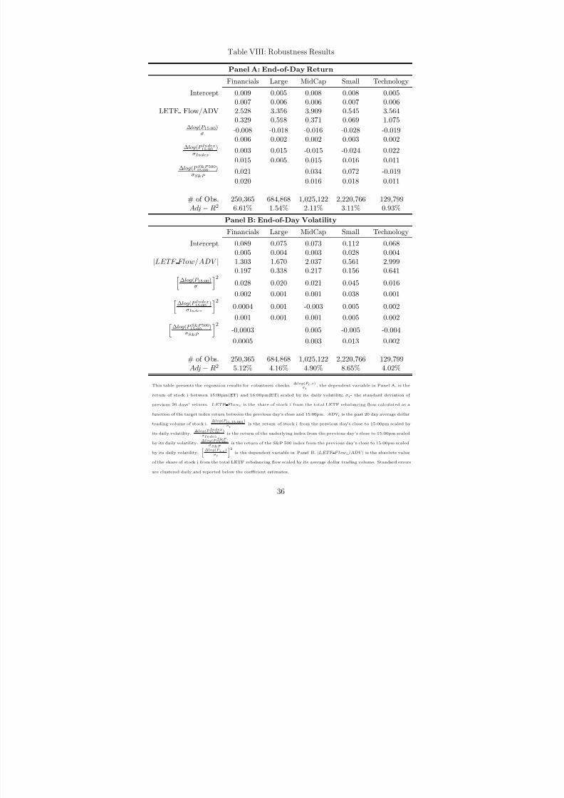
7/27/2019 Are Leveraged and Inverse ETFs the New Portfolio Insurers
http://slidepdf.com/reader/full/are-leveraged-and-inverse-etfs-the-new-portfolio-insurers 37/43
Table VIII: Robustness Results
Panel A: End-of-Day Return
Financials Large MidCap Small Technology
Intercept 0.009 0.005 0.008 0.008 0.0050.007 0.006 0.006 0.007 0.006
LETF Flow/ADV 2.528 3.356 3.909 0.545 3.5640.329 0.598 0.371 0.069 1.075
∆log(P 15:00)σ -0.008 -0.018 -0.016 -0.028 -0.019
0.006 0.002 0.002 0.003 0.002∆log(P Index
15:00 )σIndex
0.003 0.015 -0.015 -0.024 0.022
0.015 0.005 0.015 0.016 0.011∆log(P S&P 500
15:00 )σS&P
0.021 0.034 0.072 -0.019
0.020 0.016 0.018 0.011
# of Obs. 250,365 684,868 1,025,122 2,220,766 129,799Adj − R2 6.61% 1.54% 2.11% 3.11% 0.93%
Panel B: End-of-Day Volatility
Financials Large MidCap Small Technology
Intercept 0.089 0.075 0.073 0.112 0.0680.005 0.004 0.003 0.028 0.004
|LETF Flow/ADV | 1.303 1.670 2.037 0.561 2.9990.197 0.338 0.217 0.156 0.641
∆log(P 15:00)σ
20.028 0.020 0.021 0.045 0.016
0.002 0.001 0.001 0.038 0.001∆log(P Index
15:00 )σIndex
20.0004 0.001 -0.003 0.005 0.002
0.001 0.001 0.001 0.005 0.002∆log(P S&P 500
15:00 )σS&P
2-0.0003 0.005 -0.005 -0.004
0.0005 0.003 0.013 0.002
# of Obs. 250,365 684,868 1,025,122 2,220,766 129,799Adj − R2 5.12% 4.16% 4.90% 8.65% 4.02%
This table presents the regression results for robustness checks.∆log(P i ,c)
σi, the dependent variable in Panel A, is the
return of stock i between 15:00pm(ET) and 16:00pm(ET) scaled by its daily volatility, σi- the standard deviation of
previous 20 days’ returns. LETF Flowi is the share of stock i from the total LETF rebalancing flow calculated as a
function of the target index return between the previous day’s close and 15:00pm. ADV i is the past 20 day average dollar
trading volume of stock i.∆log(P (i,15:00) )
σiis the return of stock i from the previous day’s close to 15:00pm scaled by
its daily volatility.∆log(P Index15:00 )
σIndexis the return of the underlying index from the previous day’s close to 15:00pm scaled
by its daily volatility.∆log(P S&P
15:00 )
σS&P is the return of the S&P 500 index from the previous day’s close to 15:00pm scaled
by its daily volatility.
∆log(P i,c)
σi
2is the dependent variable in Panel B. |LETF F lowi/ADV | is the absolute value
of the share of stock i from the total LETF rebalancing flow scaled by its average dollar trading volume. Standard errors
are clustered daily and reported below the coefficient estimates.
36
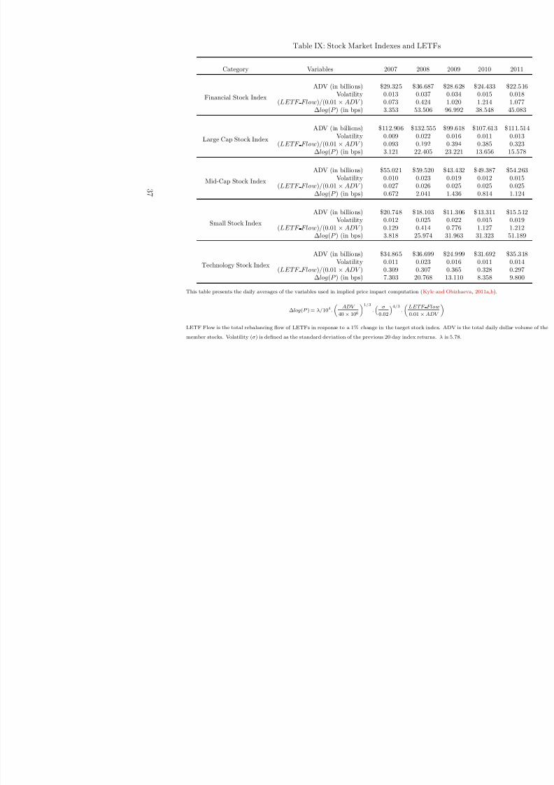
7/27/2019 Are Leveraged and Inverse ETFs the New Portfolio Insurers
http://slidepdf.com/reader/full/are-leveraged-and-inverse-etfs-the-new-portfolio-insurers 38/43
Table IX: Stock Market Indexes and LETFs
Category Variables 2007 2008 2009
Financial Stock Index
ADV (in billions) $29.325 $36.687 $28.628
Volatility 0.013 0.037 0.034 (LETF Flow)/(0.01 × ADV ) 0.073 0.424 1.020 ∆log(P ) (in bps) 3.353 53.506 96.992
Large Cap Stock Index
ADV (in billions) $112.906 $132.555 $99.618 Volatility 0.009 0.022 0.016
(LETF Flow)/(0.01 × ADV ) 0.093 0.192 0.394 ∆log(P ) (in bps) 3.121 22.405 23.221
Mid-Cap Stock Index
ADV (in billions) $55.021 $59.520 $43.432 Volatility 0.010 0.023 0.019
(LETF Flow)/(0.01 × ADV ) 0.027 0.026 0.025
∆log(P ) (in bps) 0.672 2.041 1.436
Small Stock Index
ADV (in billions) $20.748 $18.103 $11.306 Volatility 0.012 0.025 0.022
(LETF Flow)/(0.01 × ADV ) 0.129 0.414 0.776 ∆log(P ) (in bps) 3.818 25.974 31.963
Technology Stock Index
ADV (in billions) $34.865 $36.699 $24.999 Volatility 0.011 0.023 0.016
(LETF Flow)/(0.01 × ADV ) 0.309 0.307 0.365 ∆log(P ) (in bps) 7.303 20.768 13.110
This table presents the daily averages of the variables used in implied price impact computation (Kyle and Obizhaeva
∆log(P ) = λ/104.
ADV
40× 106
1/3
. σ
0.02
4/3.
LETF Flow
0.01×ADV
LETF Flow is the total rebalancing flow of LETFs in response to a 1% change in the target stock index. ADV is the t
member stocks. Volatility (σ) is defined as the standard deviation of the previous 20 day index returns. λ is 5.78.
3 7
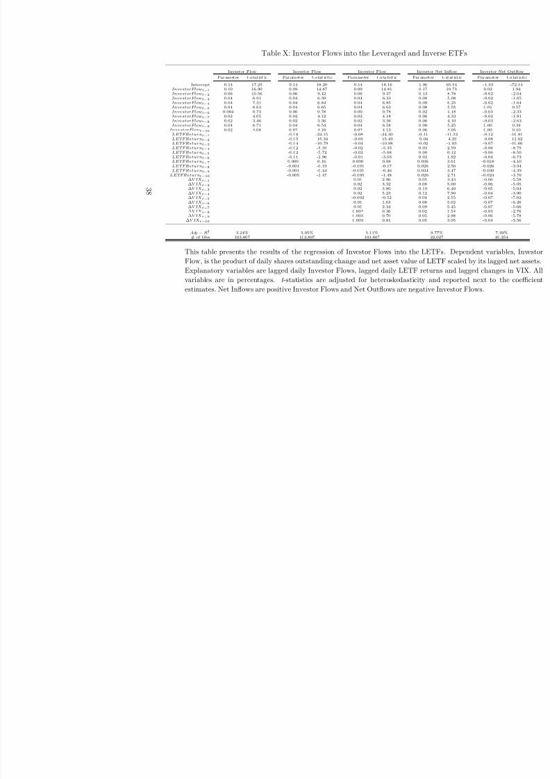
7/27/2019 Are Leveraged and Inverse ETFs the New Portfolio Insurers
http://slidepdf.com/reader/full/are-leveraged-and-inverse-etfs-the-new-portfolio-insurers 39/43
Table X: Investor Flows into the Leveraged and Inverse ETFs
Investor Flow Investor Flow Investor Flow Investor Net Inflow
Par am et er t -s tat ist ic Par am et er t -s tat is ti c Pa ra me ter t -s ta ti st ic Par am et er t- st at ist ic
Intercept 0.14 17.25 0.14 18.20 0.14 18.16 1.96 65.94 InvestorFlowt−1 0.10 16.90 0.09 14.87 0.09 14.81 0.17 10.73 InvestorFlow
t−20.06 10.56 0.06 9.42 0.06 9.37 0.13 8.78
InvestorFlowt−3 0.04 6.91 0.04 6.39 0.04 6.33 0.08 5.08 InvestorFlowt−4 0.04 7.31 0.04 6.84 0.04 6.85 0.09 6.25 InvestorFlowt−5 0.04 6.63 0.04 6.65 0.04 6.63 0.08 5.55 InvestorFlowt−6 0.004 0.73 0.00 0.78 0.00 0.78 0.02 1.18 InvestorFlowt−7 0.02 4.05 0.02 4.12 0.02 4.18 0.06 4.33 InvestorFlowt−8 0.02 3.46 0.02 3.36 0.02 3.36 0.06 4.10 InvestorFlowt−9 0.04 6.71 0.04 6.54 0.04 6.58 0.08 5.25
InvestorFlowt−10 0.02 4.08 0.02 4.10 0.02 4.13 0.06 4.05 LETFReturnt−1 -0.08 -24.15 -0.08 -24.30 -0.11 -11.33 LETFReturnt−2 -0.05 -15.34 -0.05 -15.49 -0.04 -4.25 LETFReturnt−3 -0.04 -10.79 -0.04 -10.98 -0.02 -1.93 LETFReturnt−4 -0.02 -5.10 -0.02 -5.33 0.03 2.59 LETFReturnt−5 -0.02 -5.72 -0.02 -5.68 0.00 0.12 LETFReturnt−6 -0.01 -2.96 -0.01 -3.03 0.02 1.92 LETFReturnt−7 0.000 0.16 0.000 0.08 0.036 3.61 LETFReturnt−8 -0.001 -0.19 -0.001 -0.17 0.026 2.56 LETFReturnt−9 -0.001 -0.44 -0.001 -0.46 0.034 3.47
LETFReturnt−10 -0.005 -1.47 -0.005 -1.48 0.026 2.71 ∆V IXt−1 0.01 2.96 0.05 3.43 ∆V IXt−2 0.02 3.32 0.08 5.00 ∆V IXt−3 0.02 3.80 0.10 6.40
∆V IXt−4 0.02 5.23 0.12 7.90 ∆V IXt−5 -0.002 -0.52 0.04 2.55 ∆V IXt−6 0.01 1.63 0.08 5.02 ∆V IXt−7 0.01 2.34 0.09 5.45 ∆V IXt−8 0.002 0.36 0.02 1.54 ∆V IXt−9 0.003 0.70 0.05 2.98
∆V IXt−10 0.003 0.81 0.05 3.05
Adj − R2 3.24% 5.05% 5.11% 9.77% # of Obs 103,807 103,807 103,807 22,027
This table presents the results of the regression of Investor Flows into the LETFs. Depen
Flow, is the product of daily shares outstanding change and net asset value of LETF scaled
Explanatory variables are lagged daily Investor Flows, lagged daily LETF returns and lag
variables are in percentages. t -statistics are adjusted for heteroskedasticity and reported
estimates. Net Inflows are positive Investor Flows and Net Outflows are negative Investor F
3 8
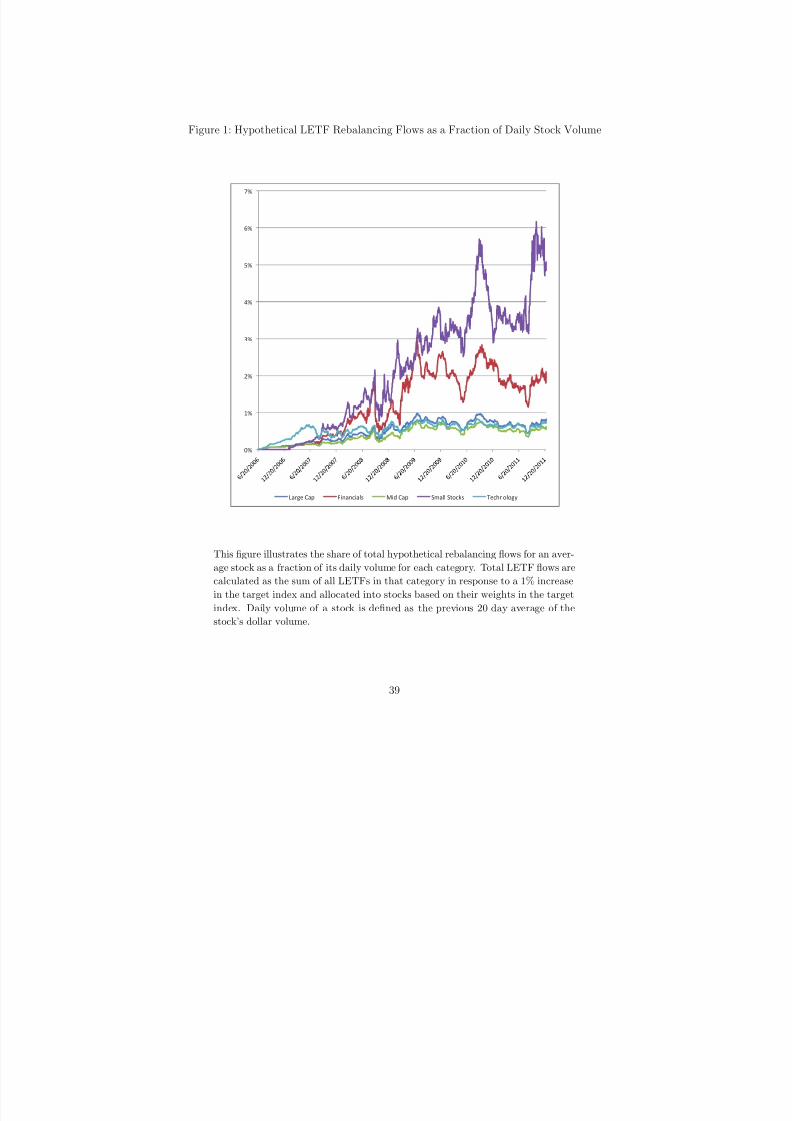
7/27/2019 Are Leveraged and Inverse ETFs the New Portfolio Insurers
http://slidepdf.com/reader/full/are-leveraged-and-inverse-etfs-the-new-portfolio-insurers 40/43
Figure 1: Hypothetical LETF Rebalancing Flows as a Fraction of Daily Stock Volume
1%
2%
3%
4%
5%
6%
7%
0%
LargeCap Financials MidCap SmallStocks Technology
This figure illustrates the share of total hypothetical rebalancing flows for an aver-age stock as a fraction of its daily volume for each category. Total LETF flows are
calculated as the sum of all LETFs in that category in response to a 1% increase
in the target index and allocated into stocks based on their weights in the target
index. Daily volume of a stock is defined as the previous 20 day average of the
stock’s dollar volume.
39
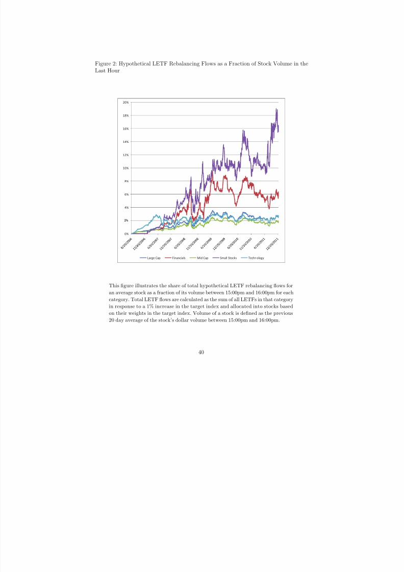
7/27/2019 Are Leveraged and Inverse ETFs the New Portfolio Insurers
http://slidepdf.com/reader/full/are-leveraged-and-inverse-etfs-the-new-portfolio-insurers 41/43
Figure 2: Hypothetical LETF Rebalancing Flows as a Fraction of Stock Volume in the
Last Hour
4%
6%
8%
10%
12%
14%
16%
18%
20%
0%
LargeCap Financials MidCap SmallStocks Technology
This figure illustrates the share of total hypothetical LETF rebalancing flows for
an average stock as a fraction of its volume between 15:00pm and 16:00pm for each
category. Total LETF flows are calculated as the sum of all LETFs in that category
in response to a 1% increase in the target index and allocated into stocks based
on their weights in the target index. Volume of a stock is defined as the previous
20 day average of the stock’s dollar volume between 15:00pm and 16:00pm.
40
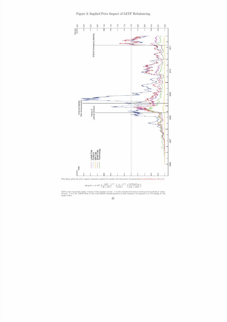
7/27/2019 Are Leveraged and Inverse ETFs the New Portfolio Insurers
http://slidepdf.com/reader/full/are-leveraged-and-inverse-etfs-the-new-portfolio-insurers 42/43
Figure 3: Implied Price Impact of LETF Rebalancing
0 . 0
0 . 2
0 . 4
0 . 6
0 . 8
1 . 0
1 . 2
1 . 4
1 . 6
1 . 8
2 . 0
2 . 2
2 . 4
2 . 6
P e r c e n
t
L a r g e
C a p
F
i n a n c e
M
i d C a p
S
m a
l l C a p
T
e c
h n o
l o g y
F a
i l u r e o
f
L
e h m a n
B r o
t h e r s
F i n a n c
i a l S t a b i l i t y
P l a n
A n n o u n c e m e n
t
E C B - G
7 E m e r g e n c y M
e e
t i n g
2 0 1 1
2 0 1 0
2 0 0 9
2
0 0 8
2 0 0 7
2 0 0 6
D a
i l y
This figure plots the price impact estimates implied by market microstructure invariance(Kyle and Obizhaeva, 2011a,b).
∆log(P ) = λ/104
.
ADV
40 × 106
1/3
.
σ
0.02
4/3
.
LETF F low
0.01 × ADV
ADV is the total daily dollar volume of the member stocks. σ is the standard deviation of the previous 20 days’ indexreturns. λ is 5.78. LETF Flow is the total LETF rebalancing flow in that category in response to a 1% change in thetarget index.
41

7/27/2019 Are Leveraged and Inverse ETFs the New Portfolio Insurers
http://slidepdf.com/reader/full/are-leveraged-and-inverse-etfs-the-new-portfolio-insurers 43/43
Figure 4: Frequency of A Late-day Large Price Move in the Financial Stock Index
0 . 0
0 . 1
0 . 2
0 . 3
0 . 4
0 . 5
0 . 6
0 . 7
0 . 8
0 . 9
1 . 0
P r o
b a
b i l i t y
L a u n c
h o
f F i r s t
F i n a n c
i a l L E T F
F a
i l u r e o
f
L e
h m a n
B r o
t h e r s
F i n a n c
i a l S t a b i l i t y
P l a n
A n n o u n c e m e n
t
E C B - G
7 E m e r g e n c y
M e e
t i n g
2 0 1 1
2 0 1 0
2 0 0 9
2 0 0 8
2 0 0 7
2 0
0 6
2 0 0 5
2 0 0 4
2 0 0 3
M o n
t h l y
This figure plots the frequency of a 1% price move in the Russell 1000 Financial Services Index b etween 3:00pm and4:00pm given that the index has already moved 1% by 3:00pm in the same direction. This measure is calculated from amonth’s trading days in which the index moved 1% by 3:00pm. More formally this frequency is:
ni=0
½ {Amplified Return}
ni=0
½ {|R3pm|≥1%}
where½ {Amplified Return} =
1 R3−4pm ≥ 1%, R3pm ≥ 1%
1 R3−4pm ≤ −1%, R3pm ≤ −1%
0 Otherwise