Are Key-Foreign Key Joins Safe to Avoid when Learning … Key-Foreign Key Joins Safe to Avoid when...

Are Key-Foreign Key Joins Safe to Avoidwhen Learning High-Capacity Classifiers?

Vraj Shah1 Arun Kumar1 Xiaojin Zhu2

1University of California, San Diego 2University of Wisconsin-Madison

{vps002, arunkk}@eng.ucsd.edu, [email protected]

ABSTRACT

Machine learning (ML) over relational data is a boomingarea of data management. While there is a lot of work onscalable and fast ML systems, little work has addressed thepains of sourcing data for ML tasks. Real-world relationaldatabases typically have many tables (often, dozens) anddata scientists often struggle to even obtain all tables forjoins before ML. In this context, Kumar et al. showed re-cently that key-foreign key dependencies (KFKDs) betweentables often lets us avoid such joins without significantlyaffecting prediction accuracy–an idea they called “avoidingjoins safely.” While initially controversial, this idea has sincebeen used by multiple companies to reduce the burden ofdata sourcing for ML. But their work applied only to lin-ear classifiers. In this work, we verify if their results holdfor three popular high-capacity classifiers: decision trees,non-linear SVMs, and ANNs. We conduct an extensive ex-perimental study using both real-world datasets and simu-lations to analyze the effects of avoiding KFK joins on suchmodels. Our results show that these high-capacity classi-fiers are surprisingly and counter-intuitively more robust toavoiding KFK joins compared to linear classifiers, refutingan intuition from the prior work’s analysis. We explain thisbehavior intuitively and identify open questions at the in-tersection of data management and ML theoretical research.All of our code and datasets are available for download fromhttp://cseweb.ucsd.edu/~arunkk/hamlet.

PVLDB Reference Format:

Vraj Shah, Arun Kumar, and Xiaojin Zhu. Are Key-Foreign KeyJoins Safe to Avoid when Learning High-Capacity Classifiers?.PVLDB, 11 (3): x-yyyy, 2017.DOI: 10.14778/3157794.3157804

1. INTRODUCTIONThe data management community has long studied how

to integrate ML with data systems [18, 12, 53]), how toscale ML [6, 32], and how to use database ideas to improveML tasks [26, 27]. However, little work has tackled the

Permission to make digital or hard copies of all or part of this work forpersonal or classroom use is granted without fee provided that copies arenot made or distributed for profit or commercial advantage and that copiesbear this notice and the full citation on the first page. To copy otherwise, torepublish, to post on servers or to redistribute to lists, requires prior specificpermission and/or a fee. Articles from this volume were invited to presenttheir results at The 44th International Conference on Very Large Data Bases,August 2018, Rio de Janeiro, Brazil.Proceedings of the VLDB Endowment, Vol. 11, No. 3Copyright 2017 VLDB Endowment 2150-8097/17/11... $ 10.00.DOI: 10.14778/3157794.3157804

pains of sourcing data for ML tasks in the first place, es-pecially, how fundamental data properties affect end-to-endML workflows [5]. In particular, applications often havemany tables connected by database dependencies such askey-foreign key dependencies (KFKDs) [37]. Thus, given anML task, data scientists almost always join multiple tablesto obtain more features [29]. But conversations with datascientists at many enterprise and Web companies revealedthat even this simple process of procuring tables is oftenpainful in practice, since different tables are often “owned”by different teams with different access restrictions. Thisslows down the ML analytics lifecycle [23]. Recent reportsof Google’s production ML systems also show that featuresthat yield marginal benefits incur high “technical debt” thatdecreases code mangeability and increases costs [42, 35].In this context, Kumar et al. [30] showed that one can of-

ten omit an entire table by exploiting KFKDs in the schema(“avoid the join”), but do so without significantly reducingML accuracy (“safely”). The basis for this dramatic capa-bility is that a KFK join creates a functional dependency(FD) between the foreign key and the features brought inby the join, which we call “foreign features.”1

Example (based on [30]). Consider a common classi-fication task: predicting customer churn. The data scien-tist starts with the main table for training (simplified forexposition): Customers (CustomerID, Churn, Gender, Age,Employer). Churn is the target, while Gender, Age, andEmployer are features. So far, this is a standard classifica-tion task. She then notices the table Employers (Employer,

State, Revenue) in her database with extra features aboutcustomers’ employers. Customers.Employer is thus a foreignkey feature connecting these tables. She joins the tables tobring in the foreign features (about employers) because shehas a hunch that customers employed by rich companies incoastal states might be less likely to churn. She then triesvarious classifiers, e.g., logistic regression or decision trees.Using learning theory, [30] revealed a dichotomy in how

safe it is to avoid a KFK join, which we summarize next. Es-sentially, ML error has two main components, bias and vari-ance; informally, bias quantifies how complex the ML modelis, while variance quantifies how tied the trained model isto the given training dataset [44]. Intuitively, more complexmodels have lower bias and higher variance; this is knownas the bias-variance trade-off. Cases with high-variance arecolloquially called overfitting [33]. Avoiding a KFK join

1While KFKDs are not the same as FDs [45], assuming fea-tures have “closed” domains, they behave essentially as FDsin the output of the join [30].

366

366-379

is unlikely to raise the bias but likely to raise the variance,since foreign keys typically have larger domains than foreignfeatures. In simple terms, avoiding joins might cause extraoverfitting. But this extra overfitting subsides with moretraining examples, a behavior that was formally quantifiedusing the powerful ML notion of VC dimension, which indi-cates the complexity of an ML model. Using this notion, [30]defined a new quantity, the tuple ratio, which is the ratio ofthe numbers of tuples of the tables being joined (customersand employers in our example). As the tuple ratio goes up,it becomes safer to avoid the join. Users can then config-ure a VC dimension-specific threshold based on their errortolerance. For simple classifiers with VC dimensions linearin the number of features (e.g., logistic regression and NaiveBayes), this threshold is as low as 20. This idea was empir-ically validated with multiple real-world datasets.

While initially controversial, the idea of avoiding joinssafely has been adopted by many data scientists, includ-ing at Facebook, LogicBlox, and MakeMyTrip [1]. Since thetuple ratio only needs the foreign table’s cardinality ratherthan the table itself, data scientists can easily decide if theywant to avoid the join or procure the extra table. However,the results in [30] had a major caveat–they applied only tolinear classifiers. In fact, their VC dimension-based analysissuggested that the tuple ratio thresholds might be too highfor high-capacity non-linear classifiers, potentially renderingthis idea inapplicable to such classifiers in practice.

In this paper, we perform a comprehensive empirical andsimulation study and analysis to verify (or refute) the appli-cability of the idea of avoiding joins safely to three popular“high-capacity” (i.e., with large or even infinite VC dimen-sions) classifiers: decision trees, SVMs, and ANNs.

Such complex classifiers are known to be prone to over-fitting [33]. Thus, the natural expectation is that avoidinga KFK join might cause more overfitting and raise the tu-ple ratio threshold compared to linear models (i.e., � 20).Surprisingly, our results show the exact opposite! We startby rerunning the experiments from [30] for such models; wealso generalize the problem slightly to allow non-categoricalfeatures. Irrespective of which model is used, the same set ofjoins usually turn out to be safe to avoid. Furthermore, onthe datasets that had joins that were not safe to avoid, thedecrease in accuracy caused by avoiding said joins (unsafely)was lower for the high-capacity classifiers. In other words,our work refutes an intuition from the VC dimension-basedanalysis of [30] and shows that these popular high-capacityclassifiers are counter-intuitively comparably or more robustto avoiding KFK joins than linear classifiers, not less.

To understand the above surprising behavior in depth, weconduct a Monte Carlo-style simulation study to stress testhow safe it is to avoid a join. We use decision trees, sincethey were the most robust to avoiding joins. We generatedata for a two-table KFK join and embed various “true”distributions for the target. This includes a known “worst-case” scenario for avoiding joins for linear classifiers (i.e.,errors blow up) [30]. We vary different properties of thedata and the true distribution: numbers of features andtraining examples, noise, foreign key domain size, and skew.In very few cases does avoiding the join cause the error torise beyond 1%. Indeed, the only scenario with much higheroverfitting was when the tuple ratio was less than 3; thisscenario arose in only 1 of the 7 real datasets. These resultsare in stark contrast to the results for linear classifiers.

Our counter-intuitive results raise new research questionsat the intersection of data management and ML theory.There is a need to formalize the effects of KFKDs/FDs onthe behavior of decision trees, SVMs, and ANNs. As a firststep, we analyze and intuitively explain the behavior of de-cision trees and SVMs. Other open questions include theimplications of more general database dependencies on thebehavior of such models and the implications of all databasedependencies for other ML tasks such as regression and clus-tering. We believe that solving these fundamental questionscould lead to new ML analytics systems functionalities thatmake it easier to use ML for data analytics.Finally, we observed two new practical bottlenecks caused

by foreign key features, especially for decision trees. First,the sheer size of their domains makes it hard to interpret andvisualize the trees. Second, some foreign key values may nothave any training examples even if they are known to be inthe domain. We adapt standard techniques to resolve thesebottlenecks and verify their effectiveness empirically.

Overall, the contributions of this paper are as follows:

• To the best of our knowledge, this is the first pa-per to analyze the effects of avoiding KFK joins onthree popular high-capacity classifiers: decision trees,SVMs, and ANNs. We present a comprehensive em-pirical study that refutes an intuition from prior workand shows that these classifiers are counter-intuitivelymore robust to avoiding joins than linear classifiers.

• We conduct an in-depth simulation study with a deci-sion tree to assess the effects of various data propertieson how safe it is to avoid a KFK join.

• We present an intuitive analysis to explain the behav-ior of decision trees and SVMs when joins are avoided.We identify open questions for research at the inter-section of data management and ML theory.

• We resolve two new practical bottlenecks with foreignkey features by adapting standard techniques.

Outline. Section 2 presents the notation, background, as-sumptions, and scope. Section 3 presents results on the realdata. Section 4 presents the simulation study. Section 5presents our analysis of the results and identifies open ques-tions. Section 6 verifies the techniques to make foreign keyfeatures more practical. We discuss related prior work inSection 7 and conclude in Section 8.

2. PRELIMINARIES AND BACKGROUND

2.1 NotationWe focus on the standard star schema KFK join setting,

which is ubiquitous in many applications, including retail,insurance, Web security, and recommendation systems [37,30, 29]. The fact table, which has the target variable, is de-noted S. It has the schema S(SID, Y,XS , FK1, . . . , FKq).A dimension table is denoted Ri (i = 1 to q) and it has theschema Ri(RIDi,XRi

). Y is the target variable (class la-bel), XS and XRi

are vectors (sequences) of features, RIDi

is the primary key of Ri, while FKi is a foreign key fea-ture that refers to Ri. We call XS home features andXRi

foreign features. Let T be the output of the star jointhat constructs the full training dataset by concatenatingthe features from all base tables. In general, its schema isT(SID, Y,XS , FK1, . . . , FKq,XR1

, . . . ,XRq ). In contrast

367

to our setting, traditional ML formulations do not distin-guish between home features, foreign keys, and foreign fea-tures. The number of tuples in S (resp. Ri) is denoted nS

(resp. nRi); the number of features in XS (resp. XRi

) isdenoted dS (resp. dRi

). Without loss of generality, we as-sume that the join is not selective, which means nS is alsothe number of tuples in T. DFKi

denotes the domain of FKi

and by definition, |DFKi| = nRi

. We call nS

nRi

the tuple ratio

for Ri. If q = 1 (only one foreign table), we drop the sub-script in the notation and use R, FK , and nR; for simplicityof exposition, we will assume q = 1 and use this notation.

2.2 Background: ML Terms and ConceptsWe intuitively explain the ML terms, concepts, models,

and theory relevant to this work and refer the interestedreader to [17, 33, 44] for a deeper background.

Basics. We focus on classification models, which need atraining dataset with labeled examples to learn the param-eters of the model. Examples include logistic regression,support vector machines (SVMs), decision trees, and artifi-cial neural networks (ANNs). Most ML models assume thatthe examples are independently and identically distributed(IID) samples from an underlying (hidden) data distribu-tion.2 A trained model’s prediction error (or accuracy) ismeasured using a test dataset not used for training. Pop-ular testing methodologies include holdout validation and(nested) k-fold cross-validation (CV). In the former, the la-beled dataset is split three-ways: one for training, one forvalidation (say, to tune hyper-parameters), and one for finaltesting. In the latter, the labeled dataset is partitioned intok folds, with k−1 folds used for training (and validation) andthe last fold used for testing; k error estimates are obtainedby cycling through each fold for testing and averaged.

Models. Logistic regression and linear SVM classify ex-amples using a hyperplane; thus, they are called linear clas-sifiers. Naive Bayes models the probability of the label byestimating the conditional probability distribution of eachfeature and multiplying them all; it can be viewed as a lin-ear classifier [33]. 1-NN simply picks the training examplenearest to a given example for prediction. Kernel SVM im-plicitly transforms feature vectors to a different representa-tion and obtains the so-called “support vectors,” which areexamples that help separate classes. An ANN applies mul-tiple layers of complex non-linear transformations to featurevectors to separate the classes. Finally, a decision tree learnsa disjunction of conjunctive predicates to predict classes.

Theory. The set of prediction functions learnable by amodel is called its hypothesis space. The test error has threecomponents: bias (approximation error), variance (estima-tion error), and noise [44]. Informally, bias quantifies theerror of a hypothetical “best” function in the hypothesisspace; it is related to the capacity of a model (how manyprediction functions it can represent), while variance quan-tifies the error of the actual prediction function obtained af-ter training relative to the hypothetical best function. Typ-ically, a more complex model (say, with more parameters)has a lower bias but higher variance; this is the bias-variancetrade-off. A classifier’s capacity can be quantified using theVapnik-Chervonenkis (VC) Dimension [44]. Intuitively, the

2Complex models known as statistical relational modelsavoid the IID assumption and handle correlated exam-ples [15]. Such models are beyond the scope of this paper.

VC dimension is the largest number of training examples themodel can classify perfectly regardless of the training labeldistribution–a capability called “shattering.” For example,logistic regression in 2 dimensions (features) can shatter atmost 3 examples due to the “XOR problem” [47]. In general,given d features, its VC dimension is d + 1. Decision trees,RBF-SVMs, and ANNs typically have large (even infinite)VC dimensions [44]; we call such models high-capacity clas-sifiers. High-capacity classifiers often tend to have highervariance than simpler linear models (with VC dimensionslinear in d), an issue colloquially called overfitting.

Feature Selection. Feature selection methods are meta-algorithms that are almost always used with an ML algo-rithm to improve accuracy and/or interpretability. Thereare three main types: (1) Wrappers: Also called subset se-lection, these methods use the ML algorithm as a black-boxto search through different feature subsets and pick the onewith the lowest error. Since optimal subset selection is NP-Hard, various heuristic wrappers are popular in practice,including sequential greedy search [16]. (2) Filters: Thesemethods assign a score to each feature (e.g., correlation co-efficient) and the top k features are selected. (3) Embedded :These methods “wire” feature selection into the ML algo-rithm, e.g., L1 or L2 regularization for logistic regression.Typically, feature selection alters the bias-variance balanceby tolerating a small increase in bias for a larger decrease invariance and thus, reducing errors overall.

2.3 Background: Avoiding KFK Joins SafelyIt was shown in [30] that the FD FK → XR has an inter-

esting and surprising implication for the bias-variance trade-off: avoiding the KFK join (i.e., omitting XR) is unlikelyto increase the bias because the hypothesis space of almostany classifier does not shrink when XR is avoided, but inthe context feature selection, avoiding the join could resultin much higher variance. The latter is because |DFK | is usu-ally much larger than the domains of the features in XR.For instance, State in our example only has 50 values butEmployer could have millions. This dichotomy led to theidea of avoiding joins safely : avoid it only if the variance isunlikely to increase much. To enable this, [30] introduced asimple decision rule with a user-settable threshold based ontheir error tolerance. The decision rule adapts a standardbound on variance from the ML literature that grows withthe VC dimension and shrinks with nS and it was simplifiedfor linear models to enable thresholding directly on the tu-ple ratio (nS/|DFK |). Thus, as the tuple ratio goes up, therewill be less overfitting, since there are more training exam-ples relative to the model’s capacity. For linear classifiers, athreshold of 20 ensured the extra overfitting was marginal.But since high-capacity classifiers are usually more proneto overfitting, this approach suggests that the tuple ratiothreshold might have to be higher for such classifiers.

2.4 Assumptions and ScopeFor the sake of tractability, we adopt some assumptions

from [30], but also drop some others to generalize the prob-lem. In particular, we drop the assumption that all featuresare categorical (finite discrete set); we allow numeric fea-tures. We focus on classification and retain the assumptionthat FK is not a (primary) key in S; otherwise, it will notbe “generalizable,” i.e., all future examples will have valuesnever seen before. In our example, CustomerID is not gener-

368

Table 1: Dataset statistics. q is the number of di-mension tables. nS is the total number of labeledexamples; since we use nested cross-validation, thetuple ratio listed is 0.6×nS/nR. N/A means that di-mension table can never be avoided, since its foreignkey feature is not generalizable.� � � � � � � � � � � � � � � � � � � � � � � � � � �� !" � # � � � � � � � � � � � � � $ � � � � � � � � �% & ' ( ) * + + ( *, � � � � � - � � � � � � � � - � - � � � � � � �. % / & % ) ( %0 � � 1 � 2 � � � � - � � � � � � � � � � � � � � � �. 3 ) * 3 ( * ' 4 56 � � � 7 " � � � � � � � � � � � � � � � - �- � � � � � � � � �8 9 9 : ; * 3 % + * ' ) ' * � � � � $ � � - � -� � � � � � � �7 � � < = � � $ $ - � � � � � � - � � � - � �� $ � � $ � � � $� � � � � $ � � � $alizable but the foreign key Employer is. We also retain theassumption that all feature domains are fully known dur-ing training; this is a standard assumptions in ML [33, 30].Handling unseen feature values is called the “cold start”issue in ML [40]. In practice, cold start is often resolvedby temporarily mapping new values to a known “Others”placeholder. As ML models are periodically retrained, fea-ture domains are expanded with such new information. Inparticular, we assume DFK is the same as the set of R.RIDvalues (new FKi values are mapped to “Others”). Our goalis not to create new ML or feature selection algorithms, noris to ascertain which algorithm yields the best accuracy orruntime. We aim to expose and analyze how KFKDs/FDsenable us to dramatically discard foreign features a prioriwhen learning some popular high-capacity classifiers.

3. EMPIRICAL STUDY WITH REAL DATAWe present results for 10 classifiers, including 7 high-

capacity ones (CART decision tree with gini, informationgain, and gain ratio; SVM with RBF and quadratic kernels;multi-layer perceptron ANN; 1-nearest neighbor), and 3 lin-ear classifiers (Naive Bayes with backward selection, logis-tic regression with L1 regularization, and linear SVM). Wealso tried a few other feature selection techniques for thelinear classifiers: Naive Bayes with forward selection and fil-ter methods and logistic regression L2 regularization. Sincethese additional linear classifiers did not provide any newinsights, we omit them due to space constraints.

3.1 DatasetsWe take the seven real datasets from [30]; these are origi-

nally from Kaggle, GroupLens, openflights.org, mtg.upf.edu/node/1671, and last.fm. Two datasets have binarytargets (Flights and Expedia); the others have multi-classordinal targets. However, to generalize the scope of theproblem studied, we retain numeric features rather than dis-cretize them as in [30]. The dataset statistics are provided inTable 1. We briefly describe the task for each dataset andexplain what the foreign features are. More details about

their schemas, including the list of all features are alreadyin the public domain (listed in [30]). All of our datasets,scripts, and code are available for download on our projectwebpage3 to make reproducibility easier.

Walmart : predict if department-wise sales will be highusing past sales (fact table) joined with stores and weath-er/economic indicators.

Flights: predict if a route is codeshared by using otherroutes (fact table) joined with airlines, source, and destina-tion airports.

Yelp: predict if a business will be rated highly using pastratings (fact table) joined with users and businesses.

MovieLens: predict if a movie will be rated highly usingpast ratings (fact table) joined with users and movies.

Expedia: predict if a hotel will be ranked highly usingpast search listings (fact table) joined with hotels and searchevents; one foreign key, viz., the search ID, has an “open”domain, i.e., past values will not be seen in the future, whichmakes it unusable as a feature.

LastFM : predict if a song will be played often using pastplay information (fact table) joined with users and artists.

Books: predict if a book will be rated highly using pastratings (fact table) joined with readers and books.

3.2 MethodologyWe perform 10-fold nested cross-validation, with a ran-

dom third of the examples in the training folds being used forvalidation during feature selection and/or hyper-parametertuning). We compare two approaches for each classifier:JoinAll, which uses all features from all base tables (thecurrent widespread practice), and NoJoin, which avoids allforeign features a priori (the approach we study). For ad-ditional insights, we also include a third approach for deci-sion trees: NoFK, which uses all features except the foreignkeys. We used the popular R packages “rpart” for the de-cision trees (but for gain ratio, we used “CORElearn”) and“e1071” for the SVMs. For the ANNs, we used the popularPython library Keras on TensorFlow. For Naive Bayes, weused the code from [30], while for logistic regression withL1 regularization, we used the popular R package “glmnet”.We used a standard grid search for hyper-parameter tuning,with the grids described in detail below.

Decision Trees: There are two hyper-parameters to tune:minsplit and cp. minsplit is the number of observations thatmust exist in a node for a split to be attempted. Any splitthat does not improve the fit by a factor of cp is pruned off.The grid is set as follows: minsplit ∈ {1, 10, 100, 103} andcp ∈ {10−4, 10−3, 0.01, 0.1, 0}

RBF-SVM : There are two hyper-parameters: C and γ.C controls the cost of misclassification. γ > 0 controls thebandwidth in the Gaussian kernel; given points xi and xj ,k(xi, xj) = exp(−γ·‖xi − xj‖

2). The grid is set as follows: C∈ {10−1, 1, 10, 100, 103} and γ ∈ {10−4, 10−3, 0.01, 0.1, 1, 10}.On Movies and Expedia, we perform an extra fine tuningstep with γ ∈ {2−7, 2−6, . . . , 23} to improve accuracy.

Quadratic-SVM : We tune the same hyper-parameters Cand γ for the polynomial kernel of degree 2: k(xi, xj) =(−γ xT

i · xj)degree. We use the same grid as RBF-SVM.

3http://cseweb.ucsd.edu/~arunkk/hamlet

369

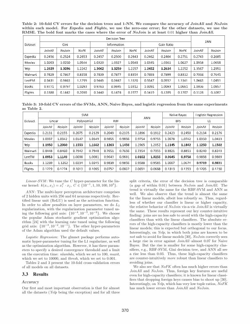
Table 2: 10-fold CV errors for the decision trees and 1-NN. We compare the accuracy of JoinAll and NoJoin

within each model. For Expedia and Flights, we use the zero-one error; for the other datasets, we use theRMSE. The bold font marks the cases where the error of NoJoin is at least 0.01 higher than JoinAll.> ? @ ? A B @ > B C D A D E F G H B B I J JK D F D L F M E H N ? @ D E F K ? D F O ? @ D EP Q R S T U U V Q P Q R S V Q W X P Q R S T U U V Q P Q R S V Q W X P Q R S T U U V Q P Q R S V Q W X P Q R S T U U V Q P Q R SY Z [ B \ D ? ] ^ _ ` a b ] ^ _ a _ ` ] ^ _ b a c ] ^ _ ` a d ] ^ _ a ] ] ] ^ _ b ` c ] ^ _ ` b _ ] ^ _ ` b ` ] ^ _ d a I ] ^ _ d ` c ] ^ _ b e af E g D B A I ^ ] _ b c I ^ ] _ a ] I ^ ] a ` ` I ^ ] c _ ] I ^ ] c _ d I ^ ] a ` e I ^ ] c ` a I ^ ] c b I I ^ ] b _ d I ^ ] h a e I ^ ] b a ei B j [ k l m n m n k l o p n q I ^ _ _ ` _ k l o p q m k l o m r n I ^ _ _ a d k l m s r m k l m q o s I ^ _ _ a _ I ^ c a b d I ^ _ h a It u v w u x y z { | } ~ � z { | } � | z { } � � } z { | } � � z { | } | | z { } � � � z { | } � � z { | } � � z { } � � ~ z { | � � } z { | � � �� ? A @ � f ] ^ h ` c I ] ^ h ` b c I ^ I _ h h ] ^ h ` ` a ] ^ h ` ` d I ^ I c _ ] ] ^ h a ` d ] ^ h a a _ I ^ I c ` I I ^ ] ` b c I ^ ] ` a I� � � � � z { � | | � z { � | � | � { z ~ � � z { � | � � z { � } � � � { z � � ~ � { z z � � � { z z � � � { z � � � � { z � � � � { z } � |� j D � � @ A ] ^ I c e e ] ^ I ` ` _ ] ^ _ ] c ] ] ^ I ` ` ] ] ^ I ` d ` ] ^ I h d d ] ^ I ` I h ] ^ I c e a ] ^ I d ] d ] ^ I I _ e ] ^ I ] e dTable 3: 10-fold CV errors of the SVMs, ANN, Naive Bayes, and logistic regression from the same experimentsas Table 2.� � � � � � � � � � � � � � � � � � � � � � � � ¡ ¢ � £ ¢ ¤ ¥ � ¡ ¦ � � � ¢ §¨ © ª � � « ¬ ® ¯ ª ° © � ® ± ² ³ ² ³ ´ ¨ µ¶ · ¸ ¹ º » » ¼ · ¶ · ¸ ¹ ¶ · ¸ ¹ º » » ¼ · ¶ · ¸ ¹ ¶ · ¸ ¹ º » » ¼ · ¶ · ¸ ¹ ¶ · ¸ ¹ º » » ¼ · ¶ · ¸ ¹ ¶ · ¸ ¹ º » » ¼ · ¶ · ¸ ¹ ¶ · ¸ ¹ º » » ¼ · ¶ · ¸ ¹½ ¾ ¿ � À © � Á Â Ã µ Ä µ Á Â Ã µ Å Å Á Â Ã Á Æ Å Á Â Ã µ Ã Ç Á Â Ã Á È Ç Á Â Ã µ Á Å Á Â µ É Ç Ê Á Â µ Ç µ Ã Á Â Ã È Ã Ä Á Â Ã È Å Á Á Â Ã µ Ä È Á Â Ã µ Æ ÊË Ì © � � µ Â Á Ä Ä Æ µ Â Á Ä È Ã µ Â Á µ È Æ µ Â Á µ È Ç Á Â Ç É Å Å Á Â Ç É Å Ê Á Â Ç Æ Å È Á Â Ç Æ Å Å µ Â Á Ê Æ É µ Â Á Æ È Ã µ Â Á Ä Å Á µ Â Á È µ ÄÍ � ® ¿ Î Ï Î Ð Ñ Ò Î Ï Ó Ò Ô Ò Î Ï Î Ñ Ñ Õ Î Ï Î Ô Ô Ó Î Ï Î Ó Ô Õ Î Ï Î Ö Ñ Ô µ Â µ Ç Ê Å µ Â Ã Á Å Ã Î Ï Î Î Ö Ñ Î Ï Î × Ö Ó Î Ï Î Ó Ñ Ò Î Ï Î Ñ Ò ÓØ � ® ° � « � Á Â É È È É Á Â É È Ê Á Á Â Æ Ç È Ã Á Â Æ Ç È É Á Â Æ Ê Å µ Á Â Æ Ê Å Ê Á Â Æ Ä Å È Á Â Æ Ä Å Å Á Â É É Ã µ Á Â É É Å µ Á Â É Ã È Á Á Â É Ã È Ä� � � £ Ù � Ú Û Ü Ý Þ ß Ú Û Ú Ú à Ý á â ã ã ä å á â ã ã å á ã â æ ç è ä ã â æ ç æ á Ú Û Ü Ú Ü é Ú Û Ü é Þ Þ Ü Û Ý ê à Þ Ü Û Ý ë Þ ì ã â æ å ä å ã â æ å ç æ² í � µ Â µ Ã Ä Ç µ Â µ Ã Ê Ã µ Â Á Ã Ä È µ Â Á Ã È Å Á Â Ç É Ä Ç Á Â Ç É Å Ê Á Â Ç Å É É Á Â Ç Å É Å µ Â Á Ê Ê Æ µ Â Á Ê Æ È Ò Ï Ð î Î Ð Ò Ï Ð × Õ ÎÙ ï ¢ ¡ ð £ � ã â á ñ ñ æ ã â á ñ ò è ã â á ã á ä ã â á ã ç ó ã â ã ò ó ñ ã â ã å ã ñ ã â ã ç ó á ã â ã ç å å ã â á ä á ä ã â á ä ó ä ã â á ñ ã ó ã â á ñ ä ã

Linear-SVM : We tune the C hyper-parameter for the lin-ear kernel: k(xi, xj) = xT

i · xj , C ∈ {10−1, 1, 10, 100, 103}.

ANN : The multi-layer perceptron architecture comprisesof 2 hidden units with 256 and 64 neurons respectively. Rec-tified linear unit (ReLU) is used as the activation function.In order to allow penalties on layer parameters, we do L2

regularization, with the regularization parameter tuned us-ing the following grid axis: {10−4, 10−3, 10−2}. We choosethe popular Adam stochastic gradient optimization algo-rithm [24] with the learning rate tuned using the followinggrid axis: {10−3, 10−2, 10−1}. The other hyper-parametersof the Adam algorithm used the default values.

Logistic Regression: The glmnet package performs auto-matic hyper-parameter tuning for the L1 regularizer, as wellas the optimization algorithm. However, it has three param-eters to specify a desired convergence threshold and a limiton the execution time: nlambda, which we set to 100, maxit,which we set to 10000, and thresh, which we set to 0.001.

Tables 2 and 3 present the 10-fold cross-validation errorsof all models on all datasets.

3.3 Results

Accuracy

Our first and most important observation is that for almostall the datasets (Yelp being the exception) and for all three

split criteria, the error of the decision tree is comparable(a gap of within 0.01) between NoJoin and JoinAll. Thetrend is virtually the same for the RBF-SVM and ANN aswell. We also observe that the trend is almost the samefor the linear models, albeit less robustly so. Thus, regard-less of whether our classifier is linear or higher capacity,the relative behavior of NoJoin vis-a-vis JoinAll is virtuallythe same. These results represent our key counter-intuitivefinding: joins are no less safe to avoid with the high-capacityclassifiers than with the linear classifiers. The absolute er-rors of the high-capacity classifiers is mostly lower than thelinear models; this is expected but orthogonal to our focus.Interestingly, on Yelp, in which both joins are known to benot safe to avoid for linear models [30], NoJoin correctly seesa large rise in error against JoinAll–almost 0.07 for NaiveBayes. But the rise is smaller for some high-capacity clas-sifiers, e.g., RBF-SVM, Gini decision tree, and ANN all seea rise less than 0.03. Thus, these high-capacity classifiersare counter-intuitively more robust than linear classifiers toavoiding joins.We also see that NoFK often has much higher errors than

JoinAll and NoJoin. Thus, foreign key features are usefuleven for high-capacity classifiers; it is known for linear classi-fiers that dropping foreign keys causes bias to shoot up [30].Interestingly, on Yelp, which has very low tuple ratios, NoFKhas much lower errors than JoinAll and NoJoin.

370

Table 4: Robustness results for discarding individualdimension tables with a Gini decision tree.ô õ ö õ ÷ ø ö ù ú û ø ü ý õ þ ÿ � ý ø ÷ � ø � û � õ � � õ � ö � õ ÷ ö � þ � ÿ ÿ ÷ ÿ � � � � � � � � � � � � � � � � � � � � � � � � � � � � � � � � �� ! ! � � ! " # # � � $ # % � � � $ " % $& � ' ( ) * * � � � # � � � � � � % � � � $ � $ � � ! " � $ � � $ # � � � $ ! ! �� & � ' ( + � � � � � # � � � � � � � � � $ % � � ! " % ! � � $ # % � � $ ! $ !Flights : NoR1 : 0.1387 NoR2 : 0.1392 NoR3 : 0.1404

NoR1, R2 : 0.1377 NoR1, R3 : 0.1379 NoR2, R3 : 0.1426

To understand the above results more deeply, we conducta “robustness” experiment by discarding dimension tablesone at a time: Table 4 presents these results for the Ginidecision tree. We see that the errors with dropping dimen-sion tables one (or even two) at a time are all still within0.01 of NoJoin in all cases, except for Yelp. Even on Yelp,the error increases significantly only when R2 (users table)is dropped, not R1. As Table 1 shows, the tuple ratio forR2 is only 3, while that for R1 is 11.2. Interestingly, thetuple ratio is similarly low (3) for R2 in Books but NoJoinerror is not much higher. Thus, the tuple ratio is only aconservative indicator: it can tell if an error is likely to risebut the error may not actually rise in some cases. Almostevery other dimension table can safely be discarded. Theresults were similar for ANN on Yelp and for the RBF-SVMon Yelp, LastFM, and Books; we skip these for brevity.

Overall, out of 14 dimension tables across the 7 datasets,we are able to safely avoid (with a tolerance of 0.01) 13 fordecision trees and ANN with a tuple ratio threshold of about3. For RBF-SVM, we were able to safely avoid 11 dimensiontables with a tuple ratio threshold being of about 6. Theseare in stark contrast to the more modest results reportedwith the linear classifiers in [30]: only 7 of the dimensiontables could be safely avoided, that too with a tuple ratiothreshold of 20. Thus, we see that the decision trees andANN need six times fewer training examples and the RBF-SVM needs three times fewer training examples than linearclassifiers to avoid significant extra overfitting when avoid-ing KFK joins. These results are counter-intuitive becausesuch complex classifiers are known to need more (not less)training examples to avoid extra overfitting.

For an interesting comparison that we use later in Section5, we also show the results for 1-NN (from “RWeka” in R)in Table 2. Surprisingly, this “braindead” classifier has sig-nificantly lower errors with NoJoin than JoinAll for mostdatasets! We discuss this behavior further in Section 5.

Hypothesis Tests. The cross-validation errors suggestthat NoJoin is not significantly worse than JoinAll for mostdatasets, especially those with high tuple ratios. We nowvalidate if the error differences are indeed statistically sig-nificant for a given error tolerance. We perform a one-tailedt-test with the ten folds’ asymmetric error differences be-tween NoJoin and JoinAll for each model on each dataset.We set the tolerance (ε) to both 0 and 0.01. The null hy-pothesis is that the error difference is not significantly higherthan ε. Figure 5 lists the number of models for which thenull hypothesis was not rejected for the standard α = 0.05confidence level and the recently recommended stricter levelof α = 0.005 [2]. We see that except on Yelp, which hasvery low tuple ratios, NoJoin is not statistically significantlyworse than JoinAll for most models (both linear and higher

Table 5: Results of the hypothesis tests., - . - / 0 . 0 1 / 2 3 0 1 / 2 3 4 3 56 7 8 9 8 : 6 7 8 9 8 8 : 6 7 8 9 8 : 6 7 8 9 8 8 :; < 1 0 = > - ? @ 5 3 5 3A B C > 0 / D D 5 3 5 3E F G H I I J KL - M N - O . P D 5 3 5 3Q - / . R A S T U UV B B W / T P 5 3 5 3R M > X Y . / Z S 5 3 5 3capacity), especially for ε = 0.01 but also for ε = 0 in manycases. For example, logistic regression on Movies and Yelphas p-values of 0.97 and 0.000026 respectively for ε = 0.01.Since the p-value for Movies is greater than the α levels, thenull hypothesis is retained. But for Yelp, the null hypothesisis rejected as the p-value is far below the α levels. Due tospace constraints, we skip the other p-values here but havereleased all the detailed results on our project webpage.

Runtimes

A key benefit of avoiding joins safely is that ML runtimes(including feature selection) could be significantly loweredfor linear models [30]. We now check if this holds for high-capacity classifiers as well by comparing the end-to-end exe-cution times (training, validation with grid search, and test-ing). Due to space constraints, we only report Gini metricfor decision trees and RBF kernel for SVMs; these were alsothe most robust to avoiding joins. All experiments (exceptfor ANN) were run on CloudLab [39]; we use a custom Open-Stack profile running Ubuntu 14.10 with 40 Intel Xeon coresand 160GB of RAM. The ANN experiments were run on acommodity laptop with Nvidia GeForce GTX 1050 GPU,16GB RAM and Windows 10. We used R version 3.2.2 andTensorFlow version 1.1.0. Figure 1 presents the results.For the high-capacity classifiers, we saw an average speedup

of about 2x for NoJoin over JoinAll. The highest speedupwas on the Movies: 3.6x for the decision tree and 6.2xfor the RBF-SVM. As for the ANN, LastFM reported thelargest speedup of 2.5x. The speedup for the linear classi-fiers were more significant, e.g., over 80x for Naive Bayeson on Movies and and about 20x for logistic regression onLastFM. These results corroborate the orders of magnitudespeedup reported in [30].

4. IN-DEPTH SIMULATION STUDYWe now dive deeper into the behavior of the decision trees

using a simulation study in which we vary the underlying“true” data distribution and sampling datasets of differentdimensions. We focus on a two-table join for simplicity.We use the decision tree, since it exhibited the maximumrobustness to avoiding KFK joins on the real data. Ourstudy comprehensively “stress tests” this robustness. Notethat our methodology is generic enough to be applicable toany other classifier too, since we only use generic notions oferror and net variance as defined in [30].

Setup and Data Synthesis. There is one dimension tableR (q = 1), and all of XS , XR, and Y are boolean (do-

371

[ \ ] ^[ \ ] [_ ` a b[ \ ] c[ \ ] d[ \ ] e[ \ ] fg \ h i j k l

m n o o_ ` a p[ \ ] [[ \ ] q[ \ ] c[ \ ] d[ \ ] eg \ h i j k l

r s t u v u w x y z s s { | u x u } ~ � � � � �� ~ } ~ � �_ ` a p[ \ ] [[ \ ] q[ \ ] c[ \ ] d[ \ ] e[ \ ] f

g \ h i j k l� � � n � � �

_ ` a p[ \ ] [[ \ ] q[ \ ] c[ \ ] d[ \ ] e[ \ ] fg \ h i j k l

� o o

[ \ ] ^[ \ ] [[ \ ] q[ \ ] c[ \ ] d[ \ ] e[ \ ] fg \ h i j k l

o � � � s � � � s v n � � �[ \ ] ^[ \ ] [[ \ ] q[ \ ] c[ \ ] d[ \ ] e

g \ h i j k l� w � u v � u t � s � z s v v u w x { � m

Figure 1: End-to-end runtimes on the real-world datasets: Walmart (W), Expedia (E), Flights (F), Yelp (Y),Movies (M), LastFM (L) and Books (B).

main size 2). We control the “true” distribution P (Y,X)and sample labeled examples in an IID manner from it. Westudy two different scenarios for what features are used to(probabilistically) determine Y : OneXr and XSXR. These sce-narios represent opposite extremes for how likely the (test)error is likely to shoot up when XR is discarded and FKis used as a representative [30]. In OneXr, a lone featureXr ∈ XR determines Y ; the rest of XR and XS are randomnoise (but note that FK will not be noise because it func-tionally determines Xr). In XSXR, all features in XS and XR

determine Y . Intuitively, OneXr is the worst-case scenariofor discarding XR because Xr is typically far more succinctthan FK, which we expect to translate to less possibility ofoverfitting with NoJoin. Note that if we use FK directly inP , XR can be more easily discarded because FK conveysmore information anyway; so, we skip such a scenario.

The following data parameters are varied one at a time:number of training examples (nS), size of foreign key domain(|DFK | = nR), number of features in XR (dR), and numberof features in XS (dS). We also sample nS

4examples each

for the validation set (for hyper-parameter tuning) and theholdout test set (final indicator of error). We generate 100different training datasets and measure the average test er-ror and average net variance (as defined in [10]) based onthe different models obtained from these 100 runs.

4.1 Scenario OneXrThe “true” distribution is set as follows: P (Y = 0|Xr =

0) = P (Y = 1|Xr = 1) = p, where p is called the probabil-ity skew parameter that controls the noise (also called Bayeserror [17]). The exact procedure for sampling examples is asfollows: (1) Construct tuples of R by sampling XR valuesrandomly (each feature value is an independent coin toss).(2) Construct the tuples of S by sampling XS values ran-domly (independent coin tosses). (3) Assign FK values toS tuples uniformly randomly from DFK . (4) Assign Y val-ues to S tuples by looking up into their respective Xr value

(implicit join on FK = RID) and sampling from the aboveconditional distribution.We compare JoinAll, NoJoin, and NoFK ; we include NoFK

for a lower bound on errors, since we know FK does not di-rectly determine Y (although indirectly it does).4 Figure 2presents the results for the test errors for varying each rele-vant data and distribution parameter, one at a time.Interestingly, regardless of the parameter varied, in almost

all cases, NoJoin and JoinAll have almost identical errors(close to the Bayes error)! From inspecting the actual de-cision trees learned in these two settings, we found that inalmost all cases, FK was used repeatedly for partitioning;seldom was a feature fromXR, includingXr, used. This sug-gests that FK can indeed act as a good representative of XR

even in this extreme case. In contrast to these results, [30]found that for linear models, the errors of NoJoin shot upcompared to JoinAll (a gap of nearly 0.05) as the tuple ra-tio starts falling below 20. In stark contrast, as Figure 2(B)shows, even for a tuple ratio of just 3, NoJoin and JoinAllhave similar errors with the decision tree. This corroboratesthe results seen for the decision tree on the real datasets(Table 2). When nS becomes very low or when |DFK | be-comes very high, the absolute errors of JoinAll and NoJoinincrease compared to NoFK. This suggests that when thetuple ratio is very low, NoFK is perhaps worth trying too.This is similar to the behavior seen on Yelp. Overall, NoJoinexhibits similar behavior as JoinAll in most cases.

We also ran this scenario for the RBF-SVM (and 1-NN);the trends were similar, except for the value of the tuple ratioat which NoJoin deviates from JoinAll. Figure 3 presentsthe results for the experiment in which we increase |DFK | =nR, while fixing everything else, similar to Figure 2(B) forthe decision tree. We see that for the RBF-SVM, the error

4In general though, NoFK could have much higher errorsif FK is part of the true distribution; indeed, NoFK hadmuch higher errors on many real datasets (Table 2).

372

� � � �� ¡¢£ ¤¤¥¤ ¦ § ¨ © ª « ¬ ® ¯ ° ±

D² ³ ± ´ µ ¶ · § ª ¸�� ¹� � º� � � ¹� � �� ¡¢£ ¤¤¥¤ »¼� � � �� ½� � � �� º ¾� � � � � � ¿ À � ¹ � ¿ À Á � � ¿ À �� ¡¢£ ¤¤¥¤ Â Ã Ä Å Æ Ç È É Ê Ç Ë Ì Í Ì Í Î Æ Ï Ë Ä Ð Ñ Æ Ò Ó Í Ô Õ

Ö¦ § ¨ © ª « ¬ × Ø µ ¶ · § ª ¸ ° ±

DÙ Ú ± ´�� ¹� � �� º Û� � �

� � Ü � �Ý ¬ Þ ß à · ·¦ ¬ Ý ¬ Þ ß¦ ¬ × Ø� �� ¡¢£ ¤¤¥¤ á¦ § ¨ © ª « ¬ ª ¶ â § « ª ¸ Þ ß ã ° ä ¯ ´ �� ¹� � �� ¹� � Ü � �� ¡¢£ ¤¤¥¤ å¦ § ¨ © ª « ¬ ª ¶ â § « ª ¸ Þ ß æ ° ä ç ´ ��

� � � ¹ �è « ¬ © ¶ © Þ · Þ â é ê ¶ « ¶ ¨ ª â ª « ¬ « è ° ë ± ® ì ´� �� ¡¢£ ¤¤¥¤ íFigure 2: Simulation results for Scenario OneXr. For all plots except (E), we fix p = 0.1. Note that nR ≡ |DFK |.(A) Vary nS, while fixing (nR, dS , dR) = (40, 4, 4). (B) Vary nR, while fixing (nS , dS , dR) = (1000, 4, 4). (C) VarydS, while fixing (nS , nR, dR) = (1000, 40, 4). (D) Vary dR, while fixing (nR, dS , dR) = (1000, 40, 4). (E) Vary p,while fixing (nS , nR, dS , dR) = (1000, 40, 4, 4). (F) Vary |DXr |, while fixing (nS , nR, dS , dR) = (1000, 40, 4, 4); all otherfeatures in XR and XS are binary.îï ð ñï ð òî ó ô ñ ñ ï ñ ï ï ñ ï ï ïõ ö ÷ ø ù ú úû ü ý ü þ ÿû ü � ��

D � � � � � � � � � � � � � � � � � � � � �D � � � îï ð òï ð !î ó " ñ ñ ï ñ ï ï#

Figure 3: Scenario OneXr simulations with the samesetup as Figure 2(B), except for (A) 1-NN and (B)RBF-SVM.

deviates when the tuple ratio falls below roughly 6. This cor-roborates its behavior on the real datasets (Table 3). The1-NN, as expected, is far less stable and the deviation startseven at a tuple ratio of 100. As Figure 4 confirms, the devi-ation in error for the RBF-SVM is due to the net variance,which helps quantify the extra overfitting. This is akin tothe extra overfitting reported in [30] using the plots of thenet variance. Intriguingly, the 1-NN sees its net variance ex-hibit non-monotonic behavior; this is likely an artifact of itsunstable behavior, since fewer and fewer training exampleswill match on FK as nR keeps rising.

Finally, we also ran this scenario with a skew in P (FK),which makes it less safe to avoid the join for linear classi-fiers [30]. But our simulations with a decision tree show thatit is robust even to foreign key skew in terms of how safe itis to avoid the join. Due to space constraints, we presentthese results in the technical report [43].

4.2 Scenario XSXRUnlike OneXr, we now create a true distribution that maps

X ≡ [XS ,XR] to Y without any noise (Bayes error). Theexact procedure for sampling examples is as follows: (1)Construct a true probability table (TPT) with entries for allpossible values of [XS ,XR] and assign a random probabilityto each entry such that the total probability is 1. (2) Foreach entry in the TPT, pick a Y value randomly and appendthe TPT entry; this ensures H(Y |X) = 0. (3) Marginalizethe TPT to obtain P (XR) and from it, sample nR = DFK

tuples for R along with an associated sequential RID value.

$% & % '% & ( ( ( % ( % % ( % % %) * + , - -. / 0 / 1 23 4 5 6 7 89 :; <=> ?@A ?BC< D%% & (% & E% & F ( ( % ( % % ( % % %G HI JK LMN OPQ ORSL T U V W X Y Z [ \ ] ^ _ ` U X a b c d e f c gh T U V W X Y Z [ \ ] ^ _ ` U X a b c d e f c gFigure 4: Average net variance in the scenario OneXr

for (A) 1-NN and (B) RBF-SVM.

(4) In the original TPT, push the probability of each entryto 0 if its XR values did not get picked for R in step 3. (5)Renormalize the TPT so that the total probability is 1 andsample nS examples (Y values do not change) and constructS. (6) For each tuple in S, pick its FK value uniformlyrandomly from the subset of RID values that map to itsXR value inR (an implicit join). We again compare JoinAll,NoJoin, and NoFK. Figure 5 presents the results.Once again, we see that NoJoin and JoinAll exhibit sim-

ilar errors in almost all cases, with the largest gap being0.017 in Figure 5(C). Interestingly, even when the tuple ra-tio is close to 1, the gap between NoJoin and JoinAll doesnot widen much. Figure 5(B)) shows that as |DFK | in-creases, NoFK remains at low overall errors, unlike bothJoinAll and NoJoin. But as we increase dR or dS , the gapbetween JoinAll/NoJoin and NoFK narrows because evenNoFK does not have enough training examples. Of course,all gaps virtually disappear as the number of training ex-amples increases, as shown by Figure 5(A). Overall, NoJoinagain exhibits similar behavior as JoinAll.

4.3 Scenario RepOneXrWe now present results for a new simulation scenario that

is a slight twist on OneXr: the tuples of R are constructedby replicating the value of Xr sampled for a tuple to createall the other features in XR. That is, XR of an example isjust the same value repeated dR times. Note that the FDFK → XR implies there are at least as many unique FKvalues as XR values. Thus, by increasing |DFK | relativeto dR, we hope to increase the chance of the model getting

373

ii j i kl m ni j o k n p q n lr st uv wxyz {{|{l m li j }i j ~l m � o o i o i i o i i ir st uv wxyz {{|{ ��li j }l m p i j � � i k j � � � o j � � ~� � � � � � �� r st uv wxyz {{|{ � � � � � � � � � � � � � � � � � � � � � � � � � � ¡¢ £ ¤ ¥ ¦ § ¨ © ª « ¬ ® ¯ ¤ § ° ± ²D³ ´ ² µ � � � � � � � � � � � � � � � � � � ¶ � · ¸ ¡ ii j }l m pi j ¹ n p q n lr st uv wxyz {{|{ º� � � � � � � � � � � � � � � � � � » � · ¼ ¡

Figure 5: Simulation results for Scenario XSXR. The parameter values varied/fixed are the same as in Figure 2(A)-(D).

½¾ ¿ ¾ À¾ ¿ Á½ Â Ã Ä Á Å Á Á Á ÅÆ ÇÈ ÉÊ ËÌÍÎ ÏÏÐÏ ÑÆ ÇÈ ÉÊ ËÌÍÎ ÏÏÐÏ Ò Ó Ô Õ Ö × Ø Ù Ù Ö Ú Û Ó × Ö Ü Ý Þ ß à á â ã Ò Ó Ô Õ Ö × Ø Ù Ù Ö Ú Û Ó × Ö Ü Ý Þ ß à á â ã½¾ ¿ ¾ À¾ ¿ Á½ Â Ã Ä Á Å Á Á Á Åä Ø Ý Þ å æ æç è é è ê ëç è ì íîFigure 6: Scenario RepOneXr simulations for deci-sion tree. (A) Vary dR while fixing (nS , nR, dS) =(1000, 40, 4). (B) Vary dR while fixing (nS , nR, dS) =(1000, 200, 4). ïð ñ òï ó ô ò õ ò ò ò õö ÷ø ùú ûüýþ ÿÿ�ÿ �ö ÷ø ùú ûüýþ ÿÿ�ÿ � � � � � � � � � � � � � � � � � � � � � � � � � � � � � � � � � � � � � �ïð ñ ð �ð ñ òï ó � � ò õ ò ò ò õ� � � � � �� !Figure 7: Scenario RepOneXr simulations with samesetup as Figure 6, except for RBF-SVM.

“confused” with NoJoin. Our goal is to see if this widensthe gap between JoinAll and NoJoin.

Figure 6 presents the results for the two experiments ondecision trees where (A) has a high tuple ratio of 25 and(B) has a low tuple ratio of 5. Once again, JoinAll andNoJoin exhibit similar errors in both the cases. The sameexperiment’s results with RBF-SVM and 1-NN are shownin Figure 7) and Figure 8 respectively. For the RBF-SVM,NoJoin has higher errors at the tuple ratio of 5 but not 25,while for the 1-NN, NoJoin has higher errors in both cases.

5. ANALYSIS AND OPEN QUESTIONS

5.1 Explaining the ResultsWe now intuitively explain the surprising behavior of de-

cision trees and RBF-SVMs with NoJoin vis-a-vis JoinAll.We first ask: Does NoJoin compromise the “generalizationerror”? The generalization error is the difference of the testand train errors. Tables 6 and 7 list the train errors (aver-aged across the 10 folds). JoinAll and NoJoin are remark-ably close for the decision trees (except for Yelp, of course).The absolute generalization errors are often high, e.g., trainerror is almost 0 on Flights with RBF-SVMs but test errorsare about 0.08, but this is orthogonal to our focus–we onlynote that NoJoin does not increase this generalization er-ror significantly. The same is true for all the decision trees.Thus, avoiding the KFK joins safely did not significantlyaffect the generalization errors the high-capacity classifiers.

Returning to 1-NN, Table 2 showed that it has similar er-rors as RBF-SVM on some datasets. We now explain whythis comparison is useful: RBF-SVM behaves similar to 1-NN in some cases when FK is used (both JoinAll and No-

"# $ %# $ &" ' ( ) * ) ) ) *+ , - . / 0 01 , + , - .2 3 4 56 78 9: ;<=> ??@? A6 78 9: ;<=> ??@? 2 B C D E F 3 G G E H I B F E J K L M N O P Q 2 B C D E F 3 G G E H I B F E J K L M N O P Q"# $ )# $ %" ' R ) ) ) SFigure 8: Scenario RepOneXr simulations with samesetup as Figure 6, except for 1-NN.

Join). But this does not necessarily hurt its test accuracy.Note that FK is represented using the standard one-hotencoding for RBF-SVM and 1-NN. So, FK can contributeto a maximum distance of 2 in a (squared) Euclidean dis-tance between two examples xi and xj . But since XR isfunctionally dependent on FK, if xi.FK = xj .FK, thenxi.XR = xj .XR. So, if xi.FK = xj .FK, the only contrib-utor to the distance is XS . But in many of the datasets,since XS is empty (dS = 0), FK becomes the sole deter-miner of the distances for NoJoin. This is akin to sheermemorization of a feature’s large domain. Since we operateon features with finite domains, test examples will also haveFK from that domain. Thus, memorizing FK does nothurt generalization. While this seems similar to how deepneural networks excel at sheer memorization but still offergood test accuracy [52], the models in our setting are notnecessarily memorizing all features but rather only FK. Asimilar explanation holds for the decision tree. If XS is notempty, then it will likely play a major role in the distancecomputations and our setting becomes more similar to thetraditional single-table learning setting (no FDs).We now explain why NoJoin deviates from JoinAll when

the tuple ratio is very low for RBF-SVM. Even if xi.FK 6=xj .FK, it is possible that xi.XR = xj .XR. Suppose the“true” distribution is captured by XR (as in OneXr). If thetuple ratio is very low, there might be many FK values butthe number of distinct XR values might still be small. Inthis case, given xi, RBF-SVM (and 1-NN) is more likelyto pick an xj that minimizes the distances on XR, thus,potentially yielding lower errors. But since NoJoin doesnot have access to XR, it can only use XS and FK. So,if XS is mostly noise, the possibility of the model getting“confused” increases. To see why, if there are few other ex-amples that share xi.FK, matching on XS becomes moreimportant. Thus, a non-match on FK becomes more likely,which means a non-match on the implicit XR becomes morelikely, which in turns makes higher errors more likely. Butif there are more examples that share xi.FK, then a matchon FK is more likely. Thus, as the tuple ratio increases,the gap between NoJoin and JoinAll decreases, as Figure 3showed. Internally, RBF-SVM seems more robust to suchchance mismatches, since it learns a higher-level relationshipbetween all features compared to 1-NN. Thus, RBF-SVM is

374

Table 6: Training errors for the same experiments as Table 2. Bold font marks the cases where the error ofNoJoin is at least 0.01 higher than JoinAll.T U V U W X V T X Y Z W Z [ \ ] ^ X X _ ` `a b c b d \ e [ ^ f U V Z [ \ g U Z \ h U V Z [i j b c k l l m j i j b c m j n o i j b c k l l m j i j b c m j n o i j b c k l l m j i j b c m j n o i j b c k l l m j i j b cp q r X s Z U t u v w x y t u v w z { t u v | | t t u v w w x t u v w | y t u v | w v t u v w y y t u v w y w t u v z } { t t~ [ � Z X W v u t t } { v u t t } { v u t w z | v u t v t | v u t v v � v u t y w y v u t v w y v u t v z w v u t y y v v u t y w | v u t w x t� � � � _ � � � � � _ � � � � � _ � � _ � � _ � � � � � _ � � � � _ _ � � � � � � � � � � � � � � � � � _ � � � � � _ � � � � � _ � _ � � �� U � f U ^ V t u z } } � t u z } | x t u { x v x t u z } | x t u z } w | t u { x � { t u z } z } t u z } | x t u { v z | t u z t w y t u z t y {� � � � � � � � � _ � � � � � _ � � _ � � � � � � � � _ � � � � � _ � � _ � _ � � � � � � � � � � � � � � � _ � _ � � � _ � � _ � � _ � � _ � �� [ [ � W t u { w } � t u { w w t t u { � t � t u { z y t t u { z y t t u { � x | t u { � y z t u { � y } t u � } v z v u t z t v v u t y w t� � Z ¡ V W t u t t t w t u t t t y t u t v x v t u t t t { t u t t t z t u t t z � t u v x w z t u v x y } t u v x | v t tTable 7: Training errors for the same experiments as Table 3. Bold font marks the cases where the error ofNoJoin is at least 0.01 higher than JoinAll.¢ £ ¤ £ ¥ ¦ ¤ § ¨ © ª « « ¬ ® ¯ ° ± ² ° ³ ´ µ ¶ · ³ ¸ · ¹ º ° ¶ » ° ³ ³ · µ ¼½ ¾ ¿ ¦ £ À Á Â Ã Ä ¿ Â Å ¾ £ Ã Æ Ç È Ç È É ½ ÊË Ì Í Î Ï Ð Ð Ñ Ì Ë Ì Í Î Ë Ì Í Î Ï Ð Ð Ñ Ì Ë Ì Í Î Ë Ì Í Î Ï Ð Ð Ñ Ì Ë Ì Í Î Ë Ì Í Î Ï Ð Ð Ñ Ì Ë Ì Í Î Ë Ì Í Î Ï Ð Ð Ñ Ì Ë Ì Í Î Ë Ì Í Î Ï Ð Ð Ñ Ì Ë Ì Í ÎÒ Ó Ô ¦ Õ ¾ £ Ö × Ø Ö Ù Ú Ö × Ø Ö Û Ù Ö × Ê Ü Ù Ý Ö × Ê Ü Þ Þ ß à á â á ã ß à ä ß á å Ö × Ê æ æ Ö Ö × Ê æ æ Ý Ö × Ø Ù Þ Ö Ö × Ø Ù Þ Ü Ö × Ø Ö Þ æ Ö × Ø Ö Þ Ú© µ ¯ · ° ³ ç è é ç ê ë ç è é ç ì ç é è ë í î ç é è ë í ï ì é è ë ì í î é è ë ð ç í é è ë î î í é è ë î ï ç ç è é ï ê ð ç è é ï ì é ç è é ç î ñ ç è é ç ð ñò ¦ Ã Ô Ê × Ê Ø Þ Ú Ê × Ê Ø Ù Ü á à ß ó ã ó á à ß â å â á à ß å ô ã á à ß â ä å Ê × Ê æ Þ Ü Ê × Ê æ Ý Ü á à ß õ å ä á à á ß ó á á à á ß ô á á à á á ó ãö £ Ã Å £ À ¤ Ö × Ú Ø Þ Ý Ö × Ú Ø Û Ê Ö × æ æ Þ Ø Ö × æ æ Þ Þ Ö × æ Ý Þ Û Ö × æ Ý Û Ø Ö × Û Ü Þ Û Ö × Û Ü Þ Ê Ö × Ú Þ Ý Ê Ö × Ú Þ Þ Ù Ö × Ú Ö Ø Ú Ö × Ú Ö æ æ½ £ ¥ ¤ È ÷ á à ß ô ø á á à ß õ å ó Ö × Ü Ú Ù Û Ö × Ü Ú Ù Ö Ö × Ü Ý Þ Ê Ö × Ü Ý Û Û Ö × Ü Ú Ý Ú Ö × Ü Ú Þ Ø Ö × Ü Ø Ý Ø Ö × Ü Ø Þ Ù Ö × Ü Ý Ý æ Ö × Ü Ý Û ØÇ Â Â ù ¥ Ê × Ö æ Ù æ Ê × Ö æ Û Ê á à ß ß õ ã á à ß ß õ â Ö × Ü Þ Ù Ý Ö × Ü Þ Þ æ Ö × Ü Ù Ù Ú Ö × Ü Ù Ý Þ Ê × Ö Ø Ù Þ Ê × Ö Ø Ý Þ Ö × Ü Ý Ù Û Ö × Ü Ý Û ÜÈ Ã ¾ ú û ¤ ¥ Ö × Ö Ú æ Ý Ö × Ö Ü Ê Ý Ö × Ö Ê Ú Ü Ö × Ö Ê Ü Ö Ö Ö Ö × Ö Ý Þ Ê Ö × Ö Þ Ö Ö Ö × Ê Ø Ý Û Ö × Ê Ø Ú Þ Ö × Ö Ü æ Ê Ö × Ê Ö Ø Úmore robust to avoiding joins at lower tuples ratios com-pared to 1-NN.

Finally, the decision tree’s internal feature selection andpartitioning seems to make it robust to noise from manyfeatures. Suppose again the “true” distribution is similar toOneXr. Since FK already encodes all information that XR

provides, the tree almost always uses FK in its partition-ing, often multiple times. This is not necessarily “bad” fortest accuracy because test examples share DFK . But whenthe tuple ratio is extremely low, the chance of XS “confus-ing” the tree against the information FK provides goes up,potentially leading to higher errors with NoJoin. JoinAll es-capes such a confusion due to XR. If XS is empty, then FKwill almost surely be used for partitioning. But with veryfew training examples per FK value, the chance of sendingit to a wrong partition goes up, leading to higher errors. Itturns out that even with just 3 or 4 training examples perFK value, such issues get mitigated. Thus, decision treesseem even more robust to avoiding joins.

5.2 Open Research QuestionsWhile our analysis intuitively explains the behavior of de-

cision trees and RBF-SVMs, there are many open questionsfor research. Is it possible to quantify the probability ofwrong partitioning with a decision tree as a function of thedata properties? Is it possible to quantify the probabilityof mismatched examples being picked by RBF-SVM? Whydoes the theory of VC dimension predict the opposite of the

observed behavior with these models? How do we quan-tify their generalization if memorization is allowable andwhat forms of memorization are allowed? Answering thesequestions would provide deeper insights into the effects ofKFKDs/FDs on such classifiers. It could also yield moreformal mechanisms to characterize when avoiding joins isfeasible beyond just looking at tuple ratios.There are database dependencies more general than FDs:

embedded multi-valued dependencies and join dependen-cies [45]. How do these dependencies among features af-fect ML models? There are also conditional FDs, whichsatisfy FD-like constraints among subsets of rows [45]; howdo such data properties affect ML models? Finally, Arm-strong’s axioms imply that foreign features can be dividedinto arbitrary subsets before being avoided; this opens up anew trade-off space between avoiding XR and using it XR.How do we quantify this trade-off and exploit it? Answer-ing these questions would open up new connections betweendata management and ML theory and potentially enablenew functionalities for ML analytics systems.

6. MAKING FK FEATURES PRACTICALWe now discuss two key practical issues caused by a large

|DFK | and study how standard techniques can be adapted toresolve them. Unlike prior work on handling large-domainregular features [8], foreign key features are distinct, sincethey have coarser-grained side information available in for-eign features, which can be exploited.

375

ü ý þÿ � � �ü ý þ �ÿ � � � � þ � � �� ý ü �� ÿ �� ý þ� � � � � þ � � �� ! " # � $ % �&Figure 9: Domain compression. (A) Flights. (B)Yelp.

6.1 Foreign Key Domain CompressionWhile foreign key features are clearly often useful for ac-

curacy, they could make interpretability difficult. For exam-ple, it is hard to visualize a decision tree that uses a foreignkey feature with 1000s of values. Thus, we consider a simpletechnique from the ML literature to mitigate this issue: lossycompression. Essentially, FK with domain DFK is recodedas [m] (where m = |DFK |). Given a user-specified positiveinteger “budget” l � m, we want a mapping f : [m] → [l].

A standard unsupervised method to construct f is therandom hashing trick [48], i.e., randomly map from [m] to[l]. We also try a simple supervised method based on filter-based feature selection that we call the Sort-based method.It preserves more of the information contained in FK aboutY . It is a greedy approach in which we sort DFK based onH(Y |FK = z), z ∈ DFK , compute the differences amongadjacent pairs of values, and pick the boundaries corre-sponding to the top l−1 differences (ties broken randomly).This gives us an l-partition of DFK . The intuition is thatby grouping FK values that have comparable conditionalentropy, H(Y |f(FK)) is unlikely to be much higher thanH(Y |FK). Note that the lower H(Y |FK) is, the more in-formative FK is to predict Y .We empirically compare the above two heuristics using

two real datasets for the Gini decision tree with NoJoin.Our methodology is as follows. We use the training parti-tion to construct f and then compress FK for the wholedataset. We then use the validation partition and obtaincross-validation errors as before. For random hashing, wereport the average across five runs. Figure 9 presents theresults. On Yelp, both Random and Sort-based have com-parable errors although Sort-based is marginally higher, es-pecially as l increases. But on Flights, the gap is larger forsome values of l although the gap narrows as the l increases.The test error with the whole DFK (l = m) for NoJoinon Flights was 0.14 (see Table 2). Thus, it is surprisingto see an error of only about 0.18 even with such high do-main compression. Even more surprisingly, the test erroron Yelp goes down after domain compression from 1.31 toabout 1.22. Overall, these results suggest that FK domaincompression, especially with Sort-based, is a promising wayto resolve the large-domain issue rather than dropping FK.

6.2 Foreign Key SmoothingAnother issue caused by a large |DFK | is that some FK

values might not arise in the train set but arise in the test setor during deployment. This is not the cold start issue, sinceall FK values are from within the closed DFK , but rather anissue of there not being enough labeled examples to cover allof DFK well. Typically, this issue is handled using smooth-ing, e.g., Laplacian smoothing for Naive Bayes by adding apseudocount of 1 to all frequency counts [33]. While simi-

'( ) *( ) +' , - ( ( ) . */ 0 1 2 3 4 45 0 / 0 1 25 0 6 78 9: ;< =>?@ AABA C8 9: ;< =>?@ AABA D E F F E D E F F E'( ) +( ) G' , H ( ( ) . *IFigure 10: Smoothing. (A) Hashing. (B) XR-based.

lar techniques have been studied for probability estimationusing decision trees [36], to the best of our knowledge, thisissue has not been handled in general for classification usingdecision trees. In fact, popular decision tree packages in Rsimply crash if this issue arises! Note that SVMs, ANNs,and other numeric feature space-based models do not havethis issue, since they use one-hot encoding of FK.We consider a simple solution approach: smooth by re-

assigning an FK value not seen during training to an FKvalue that was seen. The reassignment can be done in manyways but for simplicity sake, we consider only two unsuper-vised methods: random reassignment and distances usingforeign features (XR). Note that the latter is only feasi-ble in cases where the dimension tables have been procured;the idea is to use the auxiliary information in XR to smoothFK rather than just using JoinAll. We smooth using XR

as follows: given a test example with FK not seen duringtraining, obtain an FK seen during training whose corre-sponding XR feature vector has the minimum distance withthe given test example’s XR (ties broken randomly). Thedistance measure is just a sum of the l0 distance for categor-ical features (count of pairwise mismatches) and l2 distancefor numeric features (Euclidean distance).The intuition for XR-based smoothing is that if XR is

part of the “true” distribution, it may yield lower errorsthan random smoothing, but if XR is just noise, both meth-ods become similar. We empirically compare these methodsusing the OneXr simulation scenario in which a lone featureXr ∈ XR determines the target (with some Bayes error).We introduce a parameter γ that is the ratio of the numberof FK values not seen during training to |DFK |. If γ = 0,smoothing is not needed; as γ increases, more smoothing isneeded. Figure 10 presents the results. We see that XR-based smoothing yields much lower test errors for both No-Join and JoinAll. In fact, the smoothed approaches’ errorsare comparable to NoFK and the Bayes error for low valuesof γ (< 0.5). As γ gets closer to 1, the errors of XR-basedsmoothing also increase but not as much as random smooth-ing. Overall, these results suggest that one could get “thebest of both worlds” in a way: even if foreign features areavailable, rather for using them always as in JoinAll, an of-ten viable alternative is to use them as side information forsmoothing foreign key features with NoJoin, thus still yield-ing some of the runtime and usability benefits of NoJoin.

6.3 Discussion and LimitationsOur results confirm that it is often safe to avoid KFK

joins even for popular high-capacity classifiers. Thus, datascientists can use the tuple ratio rule to easily reduce theburden of data sourcing for such classifiers too, not just lin-ear models. We also showed that it is possible to avoid joinssafely regardless of whether features are categorical or nu-meric. This has a new implication for further theoreticalanalysis of our results because the analysis in [30] relied on

376

the finiteness of the hypothesis space due to all features be-ing categorical. But an infinite hypothesis space does notpreclude a finite VC dimension [44]. Extending the theoret-ical analysis to our more general setting is an open problem.While we focused on star schemas, our results can be easilyextended to snowflake schemas as well due to the transi-tivity of FDs. Our results also apply to single-table datawith an acyclic set of FDs, as noted in [30], since a BCNFdecomposition can yield a multi-table scenario.

We recap the limitations and assumptions of our workto help data scientists apply our idea in the right context.We focused only on popular classification models but ourresults hold for both binary and multi-class targets and bothcategorical and numeric features. If a foreign key is notgeneralizable (e.g., search ID in Expedia), it cannot be useddirectly as a feature and so, its corresponding join should notbe avoided. Finally, we leave it to future work to study theinterplay of our work with cold start techniques and latencytrade-offs during model serving.

7. RELATED WORKDatabase Dependencies and ML. Optimizing ML overjoins of multiple tables was studied in [29, 41, 38, 28], buttheir goal was primarily to reduce runtimes without affect-ing ML accuracy. ML over joins was also studied in [50] buttheir focus was on devising a new ML algorithm. In contrast,our work studied the more fundamental question of whetherKFK joins can be avoided safely for ML classifiers. We firstdemonstrated the feasibility of avoiding joins safely in [30]for linear models. In this work, we revisit that idea for high-capacity classifiers and also empirically verify mechanisms tomake foreign key features more practical. Embedded multi-valued dependencies (EMVDs) are database dependenciesthat are more general than functional dependencies [3]. Theimplication of EMVDs for probabilistic conditional indepen-dence in Bayesian networks was originally described by [34]and further explored by [49]. However, their use of EMVDsstill requires computations over all features in the data in-stance. In contrast, avoiding joins safely omits entire setsof features for complex ML models without performing anycomputations on the foreign features. There is a large bodyof work on statistical relational learning (SRL) to handlejoins that cause duplicates in the fact table [15]. But asmentioned before, our work focuses on the regular IID set-ting for which SRL might be an overkill.

Feature Selection. The ML and data mining communi-ties have long studied feature selection methods [16]. Ourgoal is not to design new feature selection methods nor isit compare existing ones. Rather, we study if KFKDs/FDsin the schema let us to avoid entire tables a priori for somepopular high-capacity classifiers, i.e., “short-circuiting” fea-ture selection using database schema information to reducethe burden of data sourcing. The trade-off between featureredundancy and relevancy is well-studied [16, 51, 25]. Theconventional wisdom is that even a feature that is redun-dant might be highly relevant and thus, unavoidable in themix [16]. Our work shows that, perhaps surprisingly, evenhighly relevant foreign features can be safely discarded inmany practical classification tasks for many high-capacityclassifiers. There is prior work on exploiting FDs in fea-ture selection; [46] infers approximate FDs using the datasetinstance and exploits them during feature selection, FO-CUS [4] is an approach to bias the input and reduce the

number of features, while [7] proposes a measure called con-sistency to aid in feature subset search. Our work is or-thogonal to these algorithms because they all still requirecomputations over all features, while avoiding joins safelyomits foreign features without even looking at them and ob-viously, without performing any computations on them. Tothe best of our knowledge, no feature selection method ex-hibits such a dramatic capability. Gini and information gainare known to be biased towards large-domain features indecision trees [8]. Different approaches have been studiedto resolve this issue [20]. Our work is orthogonal becausewe study how KFKDs/FDs enable us to ignore foreign fea-tures a priori safely. Even with the gain ratio score that isknown to mitigate the bias towards large-domain features,our main findings stand. Unsupervised dimensionality re-duction methods such as random hashing and PCA are alsopopular [17]. Our foreign key domain compression tech-niques for decision trees are inspired by such methods.

Data Integration. Integrating data and features from var-ious sources for ML often requires applying and adaptingdata integration techniques [31, 9], e.g., integrating featuresfrom different data types in recommendation systems [21],sensor fusion [22], dimensionality reduction during featurefusion [14], and controlling data quality during data fu-sion [11]. Avoiding joins safely can be seen as one schema-based mechanism to reduce the integration burden by pre-dicting a priori if a source table is unlikely to improve accu-racy. It is an open challenge to devise similar mechanismsfor other types of data sources, say, using other schema con-straints, ontology information, and sampling. There is alsoa growing interest in making data discovery and other formsof metadata management easier [13, 19]. Our work can beseen as a mechanism to verify the potential utility of some ofthe discovered data sources using their metadata. We hopeour work spurs more research in this direction of exploitingideas from data integration and data discovery to reduce thedata sourcing burden for ML tasks.

8. CONCLUSIONS AND FUTURE WORKIt is high time for the data management community to

look beyond just building faster ML systems and help re-duce the pains of data sourcing for ML. Understanding howfundamental data properties and schema information cansimplify end-to-end ML workflows is one promising avenuein this direction. While the idea of avoiding joins safely hasbeen adopted in practice for linear classifiers, in this com-prehensive study, we show that it works as well or betterfor popular high-capacity classifiers too. This goes againstthe intuition that high-capacity classifiers are typically moreprone to overfitting. We hope that our work spurs discus-sions and new research on simplifying data sourcing for ML.As for future work, we plan to formally analyze the effects

of KFKDs/FDs on high-capacity classifiers using learningtheory. Other interesting avenues include understanding theeffects of other database dependencies on ML, including re-gression and clustering models, and designing an automated“advisor” for data sourcing for ML tasks, especially whenthere are heterogeneous data types and sources.

Acknowledgments. This work was supported in part byFaculty Research Award gifts from Google and Opera Solu-tions. We thank Neoklis Polyzotis and the members of UCSan Diego’s Database Lab for their feedback on this work.

377

9. REFERENCES[1] Personal communications: Facebook friend

recommendation system; LogicBlox retail analytics;MakeMyTrip customer analytics.

[2] Nature News. https://www.nature.com/articles/d41586-017-02190-5.

[3] S. Abiteboul, R. Hull, and V. Vianu, editors.Foundations of Databases: The Logical Level.Addison-Wesley Longman Publishing Co., Inc.,Boston, MA, USA, 1st edition, 1995.

[4] H. Almuallim and T. G. Dietterich. EfficientAlgorithms for Identifying Relevant Features.Technical report, 1992.

[5] M. Anderson, D. Antenucci, V. Bittorf, M. Burgess,M. J. Cafarella, A. Kumar, F. Niu, Y. Park, C. Re,and C. Zhang. Brainwash: A Data System for FeatureEngineering. In CIDR, 2013.

[6] M. Boehm, M. W. Dusenberry, D. Eriksson, A. V.Evfimievski, F. M. Manshadi, N. Pansare,B. Reinwald, F. R. Reiss, P. Sen, A. C. Surve, andS. Tatikonda. SystemML: Declarative MachineLearning on Spark. PVLDB, 9(13):1425–1436, 2016.

[7] M. Dash, H. Liu, and H. Motoda. Consistency basedfeature selection. In Proceedings of the 4th Pacific-AsiaConference on Knowledge Discovery and Data Mining,Current Issues and New Applications, PAKDK, pages98–109, London, UK, UK, 2000. Springer-Verlag.

[8] H. Deng, G. Runger, and E. Tuv. Bias of importancemeasures for multi-valued attributes and solutions. InProceedings of the 21st International Conference onArtificial Neural Networks - Volume Part II,ICANN’11, pages 293–300, Berlin, Heidelberg, 2011.Springer-Verlag.

[9] A. Doan, A. Halevy, and Z. Ives. Principles of DataIntegration. Morgan Kaufmann Publishers Inc., SanFrancisco, CA, USA, 1st edition, 2012.

[10] P. Domingos. A Unified Bias-Variance Decompositionand its Applications. In Proceedings of 17thInternational Conference on Machine Learning, 2000.

[11] X. L. Dong and D. Srivastava. Big data integration.PVLDB, 6(11):1188–1189, 2013.

[12] X. Feng, A. Kumar, B. Recht, and C. Re. Towards aunified architecture for in-rdbms analytics. InProceedings of the 2012 ACM SIGMOD InternationalConference on Management of Data, SIGMOD ’12,pages 325–336, New York, NY, USA, 2012. ACM.

[13] R. C. Fernandez, Z. Abedjan, S. Madden, andM. Stonebraker. Towards Large-scale Data Discovery:Position Paper. In Proceedings of the ThirdInternational Workshop on Exploratory Search inDatabases and the Web, ExploreDB ’16, pages 3–5,New York, NY, USA, 2016. ACM.

[14] Y. Fu, L. Cao, G. Guo, and T. S. Huang. Multiplefeature fusion by subspace learning. In Proceedings ofthe 2008 International Conference on Content-basedImage and Video Retrieval, CIVR ’08, pages 127–134,New York, NY, USA, 2008. ACM.

[15] L. Getoor and B. Taskar. Introduction to StatisticalRelational Learning). The MIT Press, 2007.

[16] I. Guyon, S. Gunn, M. Nikravesh, and L. A. Zadeh.Feature Extraction: Foundations and Applications.New York: Springer-Verlag, 2001.

[17] T. Hastie, R. Tibshirani, and J. Friedman. TheElements of Statistical Learning: Data mining,Inference, and Prediction. Springer-Verlag, 2001.

[18] J. M. Hellerstein, C. Re, F. Schoppmann, D. Z. Wang,E. Fratkin, A. Gorajek, K. S. Ng, C. Welton, X. Feng,K. Li, and A. Kumar. The MADlib Analytics Libraryor MAD Skills, the SQL. PVLDB, 5(12):1700–1711,2012.

[19] J. M. Hellerstein, V. Sreekanti, J. E. Gonzalez,J. Dalton, A. Dey, S. Nag, K. Ramachandran,S. Arora, A. Bhattacharyya, and S. Das. Ground: AData Context Service. In CIDR, 2017.

[20] T. Hothorn, K. Hornik, and A. Zeileis. Unbiasedrecursive partitioning: A conditional inferenceframework. JOURNAL OF COMPUTATIONAL ANDGRAPHICAL STATISTICS, 15(3):651–674, 2006.

[21] Y. Jing, D. Liu, D. Kislyuk, A. Zhai, J. Xu,J. Donahue, and S. Tavel. Visual search at pinterest.In Proceedings of the 21th ACM SIGKDDInternational Conference on Knowledge Discovery andData Mining, KDD ’15, pages 1889–1898, New York,NY, USA, 2015. ACM.

[22] B. Khaleghi, A. Khamis, F. O. Karray, and S. N.Razavi. Multisensor data fusion: A review of thestate-of-the-art. Information Fusion, 14(1):28–44, Jan.2013.

[23] M. Kim, T. Zimmermann, R. DeLine, and A. Begel.Data Scientists in Software Teams: State of the Artand Challenges. IEEE Transactions on SoftwareEngineering, PP(99), 2017.

[24] D. P. Kingma and J. Ba. Adam: A Method forStochastic Optimization. In 3rd InternationalConference for Learning Representations (ICLR),2015.

[25] D. Koller and M. Sahami. Toward Optimal FeatureSelection. In ICML, 1995.

[26] P. Konda, A. Kumar, C. Re, and V. Sashikanth.Feature Selection in Enterprise Analytics: ADemonstration using an R-based Data AnalyticsSystem. PVLDB, 6(12):1306–1309, 2013.

[27] T. Kraska, A. Talwalkar, J. C. Duchi, R. Griffith,M. J. Franklin, and M. I. Jordan. MLbase: ADistributed Machine-learning System. In CIDR, 2013.

[28] A. Kumar, M. Jalal, B. Yan, J. Naughton, and J. M.Patel. Demonstration of Santoku: OptimizingMachine Learning over Normalized Data. PVLDB,8(12):1864–1867, 2015.

[29] A. Kumar, J. Naughton, and J. M. Patel. Learninggeneralized linear models over normalized data. InProceedings of the 2015 ACM SIGMOD InternationalConference on Management of Data, SIGMOD ’15,pages 1969–1984, New York, NY, USA, 2015. ACM.

[30] A. Kumar, J. Naughton, J. M. Patel, and X. Zhu. Tojoin or not to join?: Thinking twice about joins beforefeature selection. In Proceedings of the 2016International Conference on Management of Data,SIGMOD ’16, pages 19–34, New York, NY, USA,2016. ACM.

[31] Y. Li and A. Ngom. Data Integration in MachineLearning. In IEEE International Conference onBioinformatics and Biomedicine (BTBM), 2015.

378

[32] Y. Low, J. E. Gonzalez, A. Kyrola, D. Bickson, C. E.Guestrin, and J. Hellerstein. GraphLab: A NewFramework For Parallel Machine Learning. In UAI,2010.

[33] T. M. Mitchell. Machine Learning. McGraw Hill, 1997.

[34] J. Pearl and T. Verma. The Logic of RepresentingDependencies by Directed Graphs. In AAAI, 1987.

[35] N. Polyzotis, S. Roy, S. E. Whang, and M. Zinkevich.Data management challenges in production machinelearning. In Proceedings of the 2017 ACMInternational Conference on Management of Data,SIGMOD ’17, pages 1723–1726, New York, NY, USA,2017. ACM.

[36] F. Provost and P. Domingos. Tree Induction forProbability-Based Ranking. Machine Learning,52(3):199–215, 2003.

[37] R. Ramakrishnan and J. Gehrke. DatabaseManagement Systems. McGraw-Hill, Inc., 2003.

[38] S. Rendle. Scaling Factorization Machines toRelational Data. PVLDB, 6(5):337–348, 2013.

[39] R. Ricci, E. Eide, and C. Team. IntroducingCloudLab: Scientific Infrastructure for AdvancingCloud Architectures and Applications. ; login:: themagazine of USENIX & SAGE, 39(6):36–38, 2014.

[40] A. I. Schein, A. Popescul, L. H. Ungar, and D. M.Pennock. Methods and metrics for cold-startrecommendations. In Proceedings of the 25th AnnualInternational ACM SIGIR Conference on Researchand Development in Information Retrieval, SIGIR ’02,pages 253–260, New York, NY, USA, 2002. ACM.

[41] M. Schleich, D. Olteanu, and R. Ciucanu. Learninglinear regression models over factorized joins. InProceedings of the 2016 International Conference onManagement of Data, SIGMOD ’16, pages 3–18, NewYork, NY, USA, 2016. ACM.

[42] D. Sculley, G. Holt, D. Golovin, E. Davydov,T. Phillips, D. Ebner, V. Chaudhary, M. Young, J.-F.Crespo, and D. Dennison. Machine Learning: TheHigh Interest Credit Card of Technical Debt. InSE4ML: Software Engineering for Machine Learning(NIPS 2014 Workshop), 2014.

[43] V. Shah, A. Kumar, and X. Zhu. Are Key-Foreign

Key Joins Safe to Avoid when Learning High-CapacityClassifiers? (Technical Report).http://cseweb.ucsd.edu/~arunkk/hamlet.

[44] S. Shalev-Shwartz and S. Ben-David. UnderstandingMachine Learning: From Theory to Algorithms.Cambridge University Press, 2014.

[45] A. Silberschatz, H. Korth, and S. Sudarshan. DatabaseSystems Concepts. McGraw-Hill, Inc., New York, NY,USA, 5 edition, 2006.

[46] O. Uncu and I. Turksen. A Novel Feature SelectionApproach: Combining Feature Wrappers and Filters.Information Sciences, 177(2), 2007.

[47] V. N. Vapnik. The Nature of Statistical LearningTheory. Springer-Verlag New York, Inc., 1995.

[48] K. Weinberger, A. Dasgupta, J. Langford, A. Smola,and J. Attenberg. Feature hashing for large scalemultitask learning. In Proceedings of the 26th AnnualInternational Conference on Machine Learning, ICML’09, pages 1113–1120, New York, NY, USA, 2009.ACM.

[49] S. K. M. Wong, , C. J. Butz, and Y. Xiang. A Methodfor Implementing a Probabilistic Model as a RelationalDatabase. In Proceedings of the Eleventh conferenceon Uncertainty in artificial intelligence, 1995.

[50] X. Yin, J. Han, J. Yang, and P. S. Yu. Crossmine:Efficient classification across multiple databaserelations. In Proceedings of the 2004 EuropeanConference on Constraint-Based Mining and InductiveDatabases, pages 172–195, Berlin, Heidelberg, 2005.Springer-Verlag.

[51] L. Yu and H. Liu. Efficient Feature Selection viaAnalysis of Relevance and Redundancy. Journal ofMachine Learning Research, 5, Dec. 2004.

[52] C. Zhang, S. Bengio, M. Hardt, B. Recht, andO. Vinyals. Understanding Deep Learning RequiresRethinking Generalization. In InternationalConference on Learning Representations (ICLR),2017.

[53] Y. Zhang, W. Zhang, and J. Yang. I/O-EfficientStatistical Computing with RIOT. In DataEngineering (ICDE), 2010 IEEE 26th InternationalConference on, 2010.

379

Are Key-Foreign Key Joins Safe to Avoid when Learning … Key-Foreign Key Joins Safe to Avoid when...

Documents

Transcript of Are Key-Foreign Key Joins Safe to Avoid when Learning … Key-Foreign Key Joins Safe to Avoid when...