Are Irish House Prices Determined By

Fundamentals?

by

Patrick P. Foley, B.E., M.A.

2

Table of Contents

Page

List of Figures III Abstract IV

Acknowledgements IV

1. Introduction 5

2. Literature Review 9

3. Modelling the Fundamentals of House Prices 16

4. Empirical Results 20

5. Conclusion 32

References 34

Data Appendix 36

3

List of Figures Page

Figure 1 Real House Price Index (Base 1995.3 = 100) 6

Figure 2 Real House Price Inflation 6

Figure 3 Annual Irish Private House Completions 7

Figure 4 Ratio of Real Second-Hand House Prices (�) / Real GNDI per Head

of Population Aged (24-65) (�) 16

Figure 5 A plot of the actual log of real second-hand house prices and the

fitted values from Equation 5 for the period 1979.1-2002.2. 21

Figure 6 A plot of the residuals with two standard error bands from

Equation 5. 22

Figure 7 CUSUM Test of the Residuals from Equation 5. 23

Figure 8 Recursive Estimates of the Coefficients from Equation 1 and the

Computed Standard Error of the Regression. 23

Figure 9 Rolling Estimates of the Coefficients from Equation 1 and the

Computed Standard Error of the Regression. 24

Figure 10 Plot of the actual real second-hand house prices (logs), the fitted

values from Equation 7 and the single equation static forecast

values. 26

Figure 11 Plot of the actual log of real second-hand house prices and the fitted

values from Equation 8 for the period 1979.1-2002.2 30

4

Abstract

There has been much speculation in recent times concerning the rapid rise in Irish

house prices. Many commentators suggest that there is a speculative bubble in the

Irish housing market. However this study shows, using a basic supply and demand

model, that Irish house prices can indeed be modelled successfully using

fundamentals, provided that the model incorporates the impact on house prices of (i)

changes in the volume of bank lending over time and (ii) the recent influx of

investors into the Irish housing market. This study shows that a structural break

occurred in the Irish house price series in 1998 coinciding with the Government�s

decision to cut capital gains tax on residential property from forty percent to twenty

percent. The report also finds that the house price elasticity of income is a time-

varying parameter. The parameter is shown to be a function of the change in the

volume of bank mortgage lending.

Acknowledgements

I would like to thank Dr. John Considine, Mr. Niall O�Sullivan and Ms. Geraldine

Ryan, Department of Economics, University College Cork for their comments,

advice and assistance in the preparation of this research article. Any errors, of

course, are my own responsibility.

5

1. Introduction

National house prices have soared in Ireland over the past ten years. According to

the National House Price Index1 Irish residential house prices have increased

nationally by 286% since July 1996. The house price inflation figures for the year

ending July 2003 show that average national house prices continue to accelerate,

having increased annually by 15.6%2.

This dramatic rise in house prices has led many commentators to suggest that there

is a speculative bubble in the Irish house market. A recent article in The Economist3

argues that Irish house prices are 42% over valued. Moreover the article forecasts a

20% fall in house prices over the next four years. Figures 1 and 2 clearly illustrate

the recent phenomenal rise in real house prices.

One possible explanation for these dramatic price movements may be the efficient

adjustment in prices as the supply and demand sides of the housing market move

towards a new equilibrium. Prima facia, the recent increase in housing demand may

be easily explained by a number of macroeconomic and demographic factors, such

as: large increases in real disposable incomes; rapid employment growth; decreasing

real and nominal mortgage rates; reduced liquidity constraints and an increase in

population coupled with decreasing household sizes.

1 Compiled monthly by Permanent TSB in association with the Economic and Social Research Institute (ESRI). 2 The current average house prices reported for Ireland and Dublin are now �222,628 and �294,189 respectively. 3 Economics editor Pam Woodall�s article �House of cards� on May 31st 2003.

6

Figure 1. Real House Price Index (Base Year 1995.3 =100)

Figure 2. Real House Price Inflation

However in housing markets the transition to new equilibria is hampered by the

inability of housing supply to quickly shift due to construction lags, inter alia. In

50

100

150

200

250

300

1977 1978 1979 1980 1981 1982 1983 1984 1985 1986 1987 1988 1989 1990 1991 1992 1993 1994 1995 1996 1997 1998 1999 2000 2001 2002

Period (Quarterly Observations)

Hou

se P

rice

In

dex

Real 2nd Hand House Price Index

Real New House Price Index

-20%

-10%

0%

10%

20%

30%

40%

1978.4 1979.4 1980.4 1981.4 1982.4 1983.4 1984.4 1985.4 1986.4 1987.4 1988.4 1989.4 1990.4 1991.4 1992.4 1993.4 1994.4 1995.4 1996.4 1997.4 1998.4 1999.4 2000.4 2001.4 2002.4

Period (Quarterly Observations)

Ann

ual P

erce

ntag

e

Real 2nd Hand House Price Inflation

Real New House Price Inflation

7

fact, this inertia in the supply response to increasing housing demand may account

for much of the boom-bust characteristic that typifies many housing markets

internationally.

It could be argued that in the Irish case supply constraints have played a significant

role in inducing a speculative bubble into the Irish housing market. However,

Figure 3 suggests that the supply side of the Irish housing market has responded

quite well to increased housing demand.

Figure 3. Annual Irish Private House Completions

Kenny (1998) suggests that if investors purchase a house purely on the belief that

house prices are to rise, without any regard for the fundamental equilibrium value of

the house, then a speculative bubble may be said to exist. Therefore investors,

encouraged by observing dramatic price rises in the Irish housing market in the late

1990s, may have rushed into the market in the belief that double-digit capital returns

will continue thus forcing prices even hire.

20,98223,588

26,75630,132

35,454

39,086

43,024

46,657

51,932

17,30019,371

20,33021,777

23,23621,112

19,948 17,942

17,42517,163

15,37614,204

18,53618,472 19,301

58,121f

47,727

10,000

20,000

30,000

40,000

50,000

60,000

70,000

1978 1979 1980 1981 1982 1983 1984 1985 1986 1987 1988 1989 1990 1991 1992 1993 1994 1995 1996 1997 1998 1999 2000 2001 2002 2003

f: Forecast value, based on annual change in 1st quarter figuresSource: Housing Statistics Bulletin, March Quarter 2003, Department of the Environment, Heritage and Local Government.

8

Kenny (1998) also suggests that house price volatility is historically associated with

problems for the banking sector as well as macroeconomic instability. The

unwinding of imbalances in the Irish housing market built up over the recent years

could have a devastating impact on the Irish economy. Homeowners, investors,

homebuilders and the banking system could all be exposed to potentially

catastrophic consequences.

Therefore it is important to establish if house prices are determined purely by

fundamentals or whether they reflect a bubble in the market. Initially, a widely

used log-linear house price model based on supply and demand factors will be used

to investigate this matter. This model will then be modified to take into account (i)

the recent impact of investors on the housing market and (ii) the influence of

changes in the volume of bank mortgage lending on Irish house prices.

The structure of the rest of the report will now be outlined. Section 2 is a literature

review and examines the rationale behind the study more closely. The theoretical

and applied literature regarding bubbles in asset pricing will also be outlined with

particular emphasis being put on residential property pricing. Section 3 will outline

in more detail the econometric approach adopted in this study and the results of the

econometric analysis will be outlined and discussed in section 4. Finally section 5

will provide a brief summary of the research.

9

2. Literature Review

2.1 Modelling House Prices

Iacoviello (2001) highlights the fact that the housing market is somewhat different

then the market for other goods and services. The housing market has the following

special features:

• a house serves the dual function of commodity and investment,

• a house accounts for a much greater percentage of a household�s net worth

than other assets,

• a house has a high cost of supply,

• a house is durable,

• houses are heterogeneous

• houses can�t be easily moved,

• it is possible to raise loans using one�s house as collateral and

• there exists a well-developed second-hand market.

This implies that the housing market may be really viewed as a collection of loosely

connected markets. Kenny (1998) suggests that it may be therefore misleading to

talk of the price of housing or house prices in aggregate, but that abstraction will be

made for the purpose of this report.

Poterba (1984) and Hendry (1984), inter alia, have put forward models that equate

housing demand to housing supply. In these models house price volatility simply

reflects the movement towards a new equilibrium price following a demand or a

supply shock. Furthermore deviations from the market-clearing equilibrium price

10

are accentuated by large transaction costs and inertia in the response of housing

supply to shocks. In these models house prices are driven only by fundamentals and

any deviations are regarded as both rational and efficient. Therefore prices will

tend to mean-revert and observed house price movements will reflect a combination

of shocks and adjustment mechanisms. The adjustment mechanisms imply that

house prices will display positive autocorrelation.

An alternative to this optimal household behaviour is that the housing market is

inefficient due to the presence of a speculative bubble. A speculative bubble may be

said to exist if investors, seeking a short-term capital gain, buy houses solely on the

expectation that house price will rise without any regard for the fundamental

determinants of house prices.

Much of the early work on speculative bubbles focused on US equities, e.g. Diba &

Grossman (1988) and Froot & Obstfeld (1991). Diba & Grossman using unit root

and cointegration tests reject the presence of explosive rational bubbles in US stock

prices4. However, Froot & Obstfeld reject the hypothesis that there are no intrinsic

bubbles in US stocks, again using unit root and cointegration tests.

There have been some international studies on speculative behaviour in the housing

market. For example, Case and Shiller (1989) suggests that positive serial

correlation in real house prices indicates that the housing market is inefficient. Case

and Shiller investigated the housing markets in Atlanta, Chicago, Dallas and San

Francisco. For each city they divide their house sample in two, i.e. sample A and 4 Evans (1991) highlights that unit root and cointegration tests tend to reject the presence of periodically collapsing rational bubbles, even when Monte Carlo simulations have deliberately constructed this type of bubble.

11

sample B. Establishing a house price index they then regress the real annual change

in the real index for sample A on the 1 year lagged real annual change in the real

index for sample B and vice versa. Their coefficients are positive, substantial and

significant. Moreover, they find that information on real interest rates did not appear

to be incorporated into house prices for many of the cities.

Roche (1999) employing data from 1979.1 � 1998.4, investigated the presence of a

speculative bubble in the Irish and UK residential property market. Roche

decomposed Irish and British second hand house prices into their fundamental and

non-fundamental components. He then employed a regime-switching model

developed by van Norden (1996) to test whether speculative bubbles, fads or just

fundamentals drive house prices in Ireland and Britain.

Roche�s main findings suggest that there was a speculative bubble in Ireland in the

late 1990s. Roche estimated that Irish fundamental house prices fluctuated within 5

per cent of actual house prices up to 1996, but since 1997 the estimated bubble had

grown to over 10% of actual house prices. However, Roche estimated that the

probability of the bubble collapsing was then quite low at 2%. Roche did suggest,

however, that

�If the increased demand is not matched by supply, housing prices will

inevitably rise even further. If a bubble already exists in the market

the problem will be exacerbated and the probability of a crash will

most likely increase.� (Roche, 1999, p. 357).

12

2.2 The Consequences of House Price Volatility House prices have a tendency to go through large price fluctuations, i.e. boom-bust

cycles. In the past twenty years there have been dramatic declines in house prices in

the US, Canada, Japan, Australia, Britain and other European countries. Iacoviello

(2002) has studied house price movements in six major European countries, i.e.

France, Germany, Italy, Spain, Sweden and the UK, using Vector Autoregression

(VAR) techniques.

Iacoviello (2002) points out that in Britain real house prices rose about 60% between

1983 and 1989, peaked in 1989, and then fell by 47%, only stabilizing at the end of

1995. Simply viewing these trends do not in themselves indicate the existence of a

speculative bubble. However Roche (1999) did conclude that the UK collapse in

house prices during the late eighties was in fact attributable, in part, to the presence

of a speculative bubble.

Furthermore, Muellbauer and Murphy (1997) conclude, somewhat prophetically,

that the potential for volatility in the British housing market remained high and

given the low starting point for the house price/income ratio in the mid 1990s,

momentum gained in the upswing may exacerbate the next overshoot. In fact, real

house prices in Britain have increased 89% in the period 1995-2002, increasing by

almost 22% in 2002 alone5. Evidence of volatility, of course, does not automatically

imply the presence of a speculative bubble.

5 Economics editor Pam Woodall�s article �House of cards� on May 31st 2003.

13

Should a large speculative bubble exist in the Irish housing market, then, the

collapse of that bubble may have a catastrophic impact on homeowners, investors,

homebuilders and the banking system in Ireland. There is the clear possibility that

investors and homeowners may end up holding negative equity for a very long time

in the event of a housing price crash.

Kenny (1998) highlights the potential negative impact of a housing crash on demand

in the real economy when he suggests that a crash in house prices may cause a

serious decline in consumption due to negative wealth effects. Kenny further

suggests that Ireland with its young population is particularly susceptible to this

concern.

The country�s lending institutions are also vulnerable in the event of a drop in house

prices. Banks have faced insolvency recently in countries where there have been

dramatic crashes in house prices, e.g. Finland 1991-93, Sweden 1991-93, Germany

1995-2002, the UK 1989-1995, Japan 1991-2002 and Australia 1981-87.

Topi and Vilmunen (2001) outline the recent events that led to a financial crisis in

Finland. Finland boomed in the late eighties following the discovery of oil of its

coast. Then in 1990 the country was hit by large external negative shocks including

the collapse of the Soviet Union, its main trading partner. This was followed by an

increase in interest rates plus a major speculative attack on its currency that led to

the FIM losing 40% of its value between 1991 and 1993.

14

In this period output declined 13 % and the unemployment rate increased from 4 %

in 1991 to 20 % in 1993. Housing prices halved and stock prices fell by two-thirds.

The impact of the drop in house prices caused serious problems for the banking

system since much of the speculative investment was financed by bank lending

during the boom period in the Finnish economy.

Topi and Vilmunen (2001) compares the following five years in the Finnish

economy to the Great Depression in the US as bank lending dropped and

bankruptcies mounted. Finnish banks experienced growing liquidity and solvency

problems with the operation of many banks being taken over by agents of the

Finnish Government. In the end the government provided some credibility to the

banking system by issuing government backed loan guarantees.

Presently, one cannot envisage the Irish economy facing similar shocks, however by

their very nature shocks are rarely, if ever, anticipated, e.g. the two oil crises of the

1970s. Moreover, with monetary policy now being implemented for the Euro-zone,

as a whole, local negative demand shocks coupled with a tightening of monetary

policy could lead to a recession which may, in turn, be the catalyst for a crash in

Irish house prices.

Moreover, despite the slow down in the Irish economy, residential credit is still

increasing at 20% per annum. The Irish Central Bank are so concerned about this

matter that they have issued a letter to all lending institutions reminding them of the

need to maintain high lending standards in relation to residential property6. They

6 Central Bank�s Spring Bulletin 2003

15

have also advised that inspectors are to be sent out to ensure that lending institutions

are following correct procedures. Kenny (1998) addresses this issue when he warns

that,

�Despite such experiences, and the inherent risk associated with large

speculative movements in house prices, it is a common finding that

financial institutions do not adopt a prudential approach to lending

until it is too late.� (Kenny, 1998, p.13).

16

3. Modelling the Fundamentals of House Prices

The purchase of a house is such a large financial investment it is reasonable to

assume that house prices must be related to people�s income. Hendry (1984, p.213)

suggests a rather simple measure of affordability, i.e. the ratio of house prices to

income, as an initial gauge of house price movements. Figure 4 shows the

relationship between real second hand house prices and real gross national

disposable income per head of population, aged 24-65, for Ireland over the period

1977 to 2002.

Figure 4. Ratio of Real Second-Hand House Prices (€) / Real GNDI per Head of Population Aged 24-65 (€).

10

12

14

16

18

20

22

24

26

1977 1978 1979 1980 1981 1982 1983 1984 1985 1986 1987 1988 1989 1990 1991 1992 1993 1994 1995 1996 1997 1998 1999 2000 2001 2002

Period (Quarterly Observations)

Rat

io

Figure 4 suggests that from the late 1970s to the late 1980s houses became

increasingly more affordable. Then during the period 1987-1997 the ratio remained

remarkably steady. However since the beginning of 1998 this measure of

affordability has accelerated to unprecedented levels. The recent change in the ratio

suggests that there may be other factors influencing the ratio, such as the increased

17

numbers of investors in the housing market and/or reduced liquidity constraints. To

investigate these matters further more sophisticated modelling techniques must be

adopted.

Initially, the following model based on the demand and supply for housing will be

used to investigate whether or not house prices are determined by their

fundamentals.

Ln ph = β0 + β1 ln hs + β2 ln y + β3 ln pop. + β4 me (1)

where ph is the real second-hand house price7, hs is housing stock, y is permanent

income, pop. is the section of the population aged 24-65 and me is the expected real

mortgage rate. Similar models have been used in other studies of the housing

market, e.g. Hendry (1984); Poterba (1984); Muellbauer and Murphy (1997); Roche

(1999) and Bacon and MacCabe (2000). In estimating this model it may be assumed

that the fitted value is the fundamental price and the residuals represent the non-

fundamental price or the bubble term.

The model is estimated, using quarterly data, for real second-hand house prices. A

four-quarter moving average of GNDI per capita is used as the proxy for real

disposable income8, after Roche (1999). The proxy for housing stock is computed

by combining data on the number of households, taken from the Census of

Population, and quarterly data on private house completions, after Kenny (1998).

Population estimates are available annually and are interpolated to provide quarterly

data. A four-quarter moving average of nominal mortgage rates less actual nominal

7 The model was also estimated for new house prices, however the findings were extremely similar to those for second hand houses and so were not included in this report. 8 This data is only available annually and is interpolated to obtain quarterly data.

18

house price appreciation is used as a proxy for expected real mortgage rates9. More

detailed information on the data used is provided in the Data Appendix.

The model is initially estimated for the sample period from 1979.1 to 2002.2. These

initial results are then examined to establish whether the estimated parameters are

stable over the entire sample period. Test for structural breaks, outlined later in the

report, suggest that the parameters estimated for Equation 1 are unstable over the

sample period. This report posits two possible solutions to the problem of parameter

instability encountered with our estimation of Equation 1 over our sample period.

Firstly, it is argued that a structural break occurred in the Irish house prices series in

the first quarter of 1998. One possible cause of this structural break may be the

increased participation in the market of investors. A probable catalyst for the

entrance of investors into the market may be the reduction in capital gains tax on

profits from residential property investment from 40% to 20%. The Minister of

Finance introduced this change on the 3rd of December 199710. Equation 1 is

therefore modified through the introduction of both a differential intercept term and

a differential slope coefficient for disposable income in an attempt to model this

structural break.

Furthermore, many commentators have suggested that bank-lending practices have

fuelled movements in house prices. If this is the case then the house price elasticity

of income, i.e. β2 in Equation 1, may actually be a time-varying parameter with

9 me = a four quarter moving average of [100.ln (1+ it/4) � ∆Pt/Pt-1]. Where it is nominal annual mortgage interest rates reported quarterly and Pt is nominal house prices. 10 Investors would also have been enticed into the market by the introduction of less penal stamp duties on residential properties from the 23rd of April 1998.

19

changes in the volume of bank lending affecting the value of β2. Therefore,

assuming that

β2 = f(ln lS)

= γ0 + γ1ln lS (2)

where ln lS is the log of loans supplied11, then Equation 1 can be further modified to

incorporate the possible time-varying nature of β2.

To incorporate the possibility that a structural break occurs at the beginning of 1998

and the probable time-varying characteristics of β2 Equation 1 may be modified as

follows;

ln ph = β0 + α0Di + β1 ln hs + (γ0 + γ1ln lS ) ln y + α2 (Diln y) +

β3 ln pop. + β4 me (3)

or

ln ph = β0 + α0Di + β1 ln hs + γ0 ln y + α 2 (Diln y) + γ1(ln lS *ln y)

+ β3 ln pop. + β4 me (4)

where ph is the real house price, hs is housing stock, y is permanent income, pop.

is the section of the population aged 24-65, me is the expected real mortgage rate,

ln lS is the log of loans supplied and Di = 1 for observations from 1998.1 to 2002.2

and zero for observations in the earlier period. Equation 4 is estimated for the

period 1979.1 � 2002.2.

11 See Data Appendix for more information on data source.

20

4. Empirical Results

4.1 Estimating Equation 1

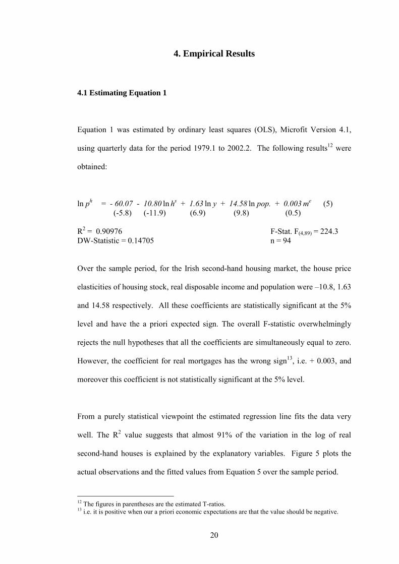
Equation 1 was estimated by ordinary least squares (OLS), Microfit Version 4.1,

using quarterly data for the period 1979.1 to 2002.2. The following results12 were

obtained:

ln ph = - 60.07 - 10.80 ln hs + 1.63 ln y + 14.58 ln pop. + 0.003 me (5) (-5.8) (-11.9) (6.9) (9.8) (0.5) R2 = 0.90976 F-Stat. F(4,89) = 224.3 DW-Statistic = 0.14705 n = 94

Over the sample period, for the Irish second-hand housing market, the house price

elasticities of housing stock, real disposable income and population were �10.8, 1.63

and 14.58 respectively. All these coefficients are statistically significant at the 5%

level and have the a priori expected sign. The overall F-statistic overwhelmingly

rejects the null hypotheses that all the coefficients are simultaneously equal to zero.

However, the coefficient for real mortgages has the wrong sign13, i.e. + 0.003, and

moreover this coefficient is not statistically significant at the 5% level.

From a purely statistical viewpoint the estimated regression line fits the data very

well. The R2 value suggests that almost 91% of the variation in the log of real

second-hand houses is explained by the explanatory variables. Figure 5 plots the

actual observations and the fitted values from Equation 5 over the sample period.

12 The figures in parentheses are the estimated T-ratios. 13 i.e. it is positive when our a priori economic expectations are that the value should be negative.

21

Figure 5. A plot of the actual log of real second-hand house prices and the fitted values from Equation 5 for the period 1979.1-2002.2.

Prima facia, Figure 5 suggests that much of the house price movements during the

period of study may be explained by changes in the fundamentals determining house

prices. In fact the graph suggests that for much of the 1990s house prices, although

rising rapidly, were undervalued. Since 1998 however it appears that house prices

have deviated above their fundamental price.

However the Durbin-Watson (DW) statistic clearly indicates the presence of strong

positive autocorrelation in the residuals. Figure 6 plots the residuals and the

presence of positive autocorrelation is clearly illustrated. The autocorrelation is not

entirely unexpected and may be due to inertia in the variables, the cobweb

phenomenon and/or specification bias14. However, the presence of such strong

autocorrelation vitiates the estimated t and F values15.

14 Ramsey�s Reset test, not reported, also suggests that the model is mis-specified. 15 Estimating the equation using the Cochrane-Orcutt method, removes the autocorrelation, but results in none of the coefficients being individually statistically significant at the 5% level.

11.1

11.3

11.5

11.7

11.9

12.1

12.3

12.5

1979 1980 1981 1982 1983 1984 1985 1986 1987 1988 1989 1990 1991 1992 1993 1994 1995 1996 1997 1998 1999 2000 2001 2002

Log

of R

eal H

ouse

Pric

es

Log of Real House Prices

Fitted Values

22

Poterba (1984) predicts that house price will have a mean-reverting tendency.

Poterba suggests that observed price movements reflect a combination of shocks and

adjustment mechanisms, the latter implying positive autocorrelations in the house

prices.

Figure 6. A plot of the residuals with two standard error bands from Equation 5.

The residuals follow an AR(1) process outlined below16, Ut = 0.0028974 + 0.93432 Ut-1 + υt (6) (0.71010) (23.2862) R2 = .85630 where Ut is the estimated residual at time t and υt is white noise.

However, taking a closer look at the residuals from Equation 5, the CUSUM and

CUSUM of Squares tests for our estimated model suggest that around 1997, i.e.

around observations 73-76, the estimated regression begins to lose precision, see

Figure 7. Furthermore, a structural break appears to occur at around 1999.2.

16 Results from Microfit, Version 4.1.

-0.25

-0.20

-0.15

-0.10

-0.05

0.00

0.05

0.10

0.15

0.20

0.25

1979 1980 1981 1982 1983 1984 1985 1986 1987 1988 1989 1990 1991 1992 1993 1994 1995 1996 1997 1998 1999 2000 2001 2002

Res

idua

ls

23

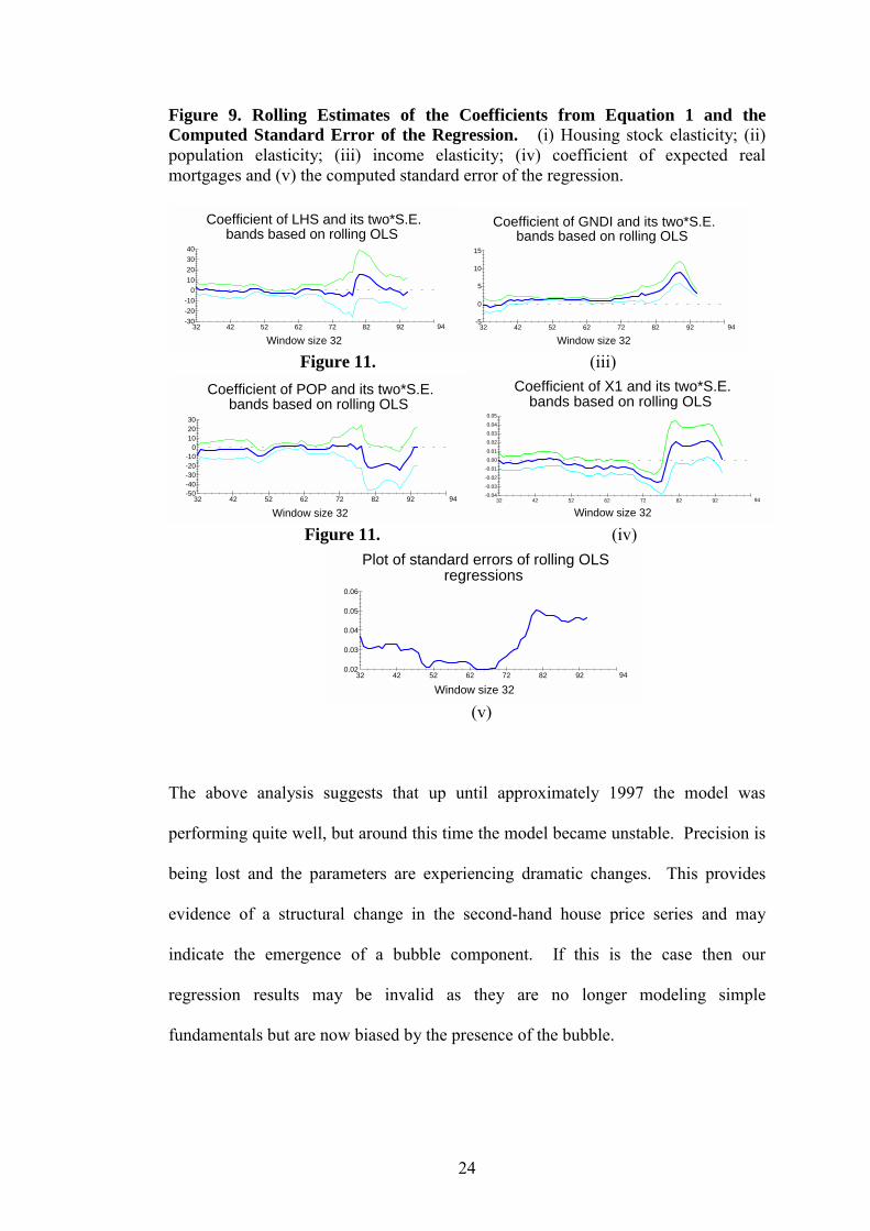
Recursive and rolling estimates of Equation 1 seem to confirm this message, see

Figures 8 and 9.

Figure 7. CUSUM test on the residuals from Equation 517.

Plot of Cumulative Sum of RecursiveResiduals

The straight lines represent critical bounds at 5% significance level

-10-20-30

01020304050

1 11 21 31 41 51 61 71 81 91 94

Plot of Cumulative Sum of Squares ofRecursive Residuals

The straight lines represent critical bounds at 5% significance level

-0.5

0.0

0.5

1.0

1.5

1 11 21 31 41 51 61 71 81 91 94

Figure 8. Recursive Estimates of the Coefficients from Equation 1 and the Computed Standard Error of the Regression. (i) Housing stock elasticity; (ii) population elasticity; (iii) income elasticity, (iv) coefficient of expected real mortgages and (v) computed standard error.

Coef. of LHS and its 2 S.E. bandsbased on recursive OLS

Observations

-10-20

01020304050

1 11 21 31 41 51 61 71 81 91 94

Coef. of GNDI and its 2 S.E. bandsbased on recursive OLS

Observations

-20

0

20

40

60

80

1 11 21 31 41 51 61 71 81 91 94

Figure 11. (iii)

Coef. of POP and its 2 S.E. bands

based on recursive OLS

Observations

-50

-100

-150

0

50

1 11 21 31 41 51 61 71 81 91 94

Coef. of X1 and its 2 S.E. bandsbased on recursive OLS

Observations

-0.02-0.04

0.000.020.040.060.080.10

1 11 21 31 41 51 61 71 81 91 94

Figure 11. (iv)

Plot of the regression standard errors

of recursive OLS

Observations

0.00

0.05

0.10

0.15

1 11 21 31 41 51 61 71 81 91 94

(v)

17 The graphs in Figures 7,8 and 9 were produced by Microfit Version 4.1.

24

Figure 9. Rolling Estimates of the Coefficients from Equation 1 and the Computed Standard Error of the Regression. (i) Housing stock elasticity; (ii) population elasticity; (iii) income elasticity; (iv) coefficient of expected real mortgages and (v) the computed standard error of the regression.

Coefficient of LHS and its two*S.E.bands based on rolling OLS

Window size 32

-10-20-30

010203040

32 42 52 62 72 82 92 94

Coefficient of GNDI and its two*S.E.bands based on rolling OLS

Window size 32

-5

0

5

10

15

32 42 52 62 72 82 92 94

Figure 11. (iii)

Coefficient of POP and its two*S.E.bands based on rolling OLS

Window size 32

-10-20-30-40-50

0102030

32 42 52 62 72 82 92 94

Coefficient of X1 and its two*S.E.bands based on rolling OLS

Window size 32

-0.01-0.02-0.03-0.04

0.000.010.020.030.040.05

32 42 52 62 72 82 92 94

Figure 11. (iv)

Plot of standard errors of rolling OLSregressions

Window size 32

0.02

0.03

0.04

0.05

0.06

32 42 52 62 72 82 92 94

(v)

The above analysis suggests that up until approximately 1997 the model was

performing quite well, but around this time the model became unstable. Precision is

being lost and the parameters are experiencing dramatic changes. This provides

evidence of a structural change in the second-hand house price series and may

indicate the emergence of a bubble component. If this is the case then our

regression results may be invalid as they are no longer modeling simple

fundamentals but are now biased by the presence of the bubble.

25

Alternatively, the structural change may be due to the influx of investors into the

market around 1998 and/or it may reflect evidence of some other form of parameter

instability, e.g. a time-varying parameter. The report will now investigate whether

or not a structural change took place in our house price series in the late 1990s.

4.2 Testing for a Structural Break

Therefore, to test for a structural break, corresponding with the Government�s

decision to reduce capital gains tax from 40% to 20%, Equation 1 was re-estimated

for the period 1979.1 to 1997.4. The newly estimated regression was used to

provide forecasts for the period 1998.1 to 2002.2 and these forecasts values were

then used to test for structural break. Equation 7 outlines the results of our

regression estimate of Equation 1 for the period 1979.1 to 1997.4.

ln ph = - 0.34 - 4.93 ln hs + 1.27 ln y + 4.89 ln pop. - 0.011 me (7) (-0.06) (-10.3) (12.4) (6.2) (-3.7) R2 = 0.88491 F-Stat. F(4,89) = 136.5 DW-Statistic = 0.82971 n = 76

Over the sample period 1979.1�1997.4 the house price elasticities of housing stock,

real disposable income and population are �4.93, 1.27 and 4.89 respectively. The

decline in these coefficients suggests that real second-hand house prices are less

sensitive to changes in these explanatory variables over the shorter sample period.

The coefficients are still statistically significant at the 5% level and have the

expected a priori sign. Again the overall F-statistic rejects the null hypotheses that

all the coefficients are simultaneously equal to zero.

26

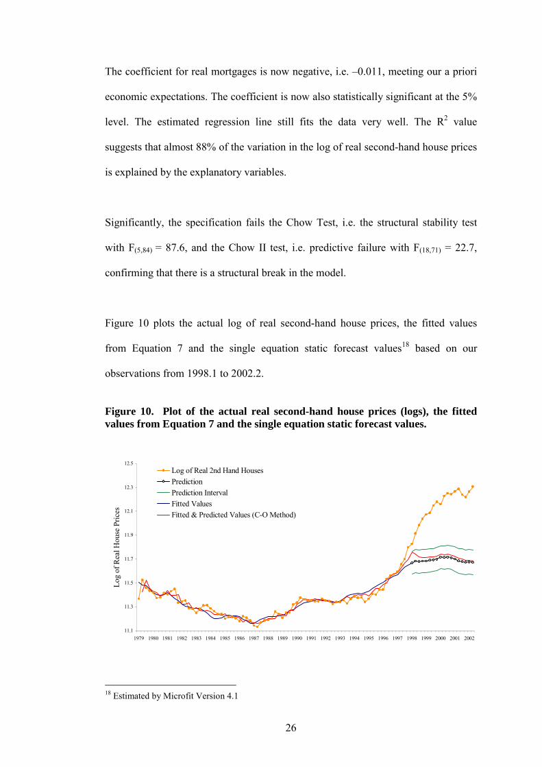
The coefficient for real mortgages is now negative, i.e. �0.011, meeting our a priori

economic expectations. The coefficient is now also statistically significant at the 5%

level. The estimated regression line still fits the data very well. The R2 value

suggests that almost 88% of the variation in the log of real second-hand house prices

is explained by the explanatory variables.

Significantly, the specification fails the Chow Test, i.e. the structural stability test

with F(5,84) = 87.6, and the Chow II test, i.e. predictive failure with F(18,71) = 22.7,

confirming that there is a structural break in the model.

Figure 10 plots the actual log of real second-hand house prices, the fitted values

from Equation 7 and the single equation static forecast values18 based on our

observations from 1998.1 to 2002.2.

Figure 10. Plot of the actual real second-hand house prices (logs), the fitted values from Equation 7 and the single equation static forecast values.

18 Estimated by Microfit Version 4.1

11.1

11.3

11.5

11.7

11.9

12.1

12.3

12.5

1979 1980 1981 1982 1983 1984 1985 1986 1987 1988 1989 1990 1991 1992 1993 1994 1995 1996 1997 1998 1999 2000 2001 2002

Log

of R

eal H

ouse

Pric

es

Log of Real 2nd Hand HousesPredictionPrediction IntervalFitted ValuesFitted & Predicted Values (C-O Method)

27

Figure 10 indicates that the fitted values of Equation 7 match the actual observations

quite well. However it is clear that the estimated parameters from Equation 7 are

not very useful in forecasting house prices for the period 1998.1 to 2002.2,

reinforcing the suggestion that there exists a structural break in the house price

series.

Also much of the serial correlation is now disappearing from the data although the

DW-statistic still suggests that positive serial correlation is still an issue. However,

adjusting for serial correlation using the Cochrane-Orcutt (C-0) method fails to alter,

to any great extent, the coefficients� values, the signs of the coefficients or their

statistical significance over the sample period 1979.1-1997.4. Obviously, therefore,

the fitted and forecasted values obtained using the C-0 estimated regression match

pretty closely the corresponding values obtained using the OLS estimated

regression. These results are also plotted in Figure 10.

The presence of serial correlation may also suggest that Equation 1 is mis-specified.

The problem may be one of omitted variable bias. As outlined in section 3, one

possible solution to this specification issue may be found in the influence that the

volume of bank mortgage lending is having on the house price elasticity of income,

i.e. Equation 2.

Therefore to take into consideration both the structural brake in the house price

series and the time-varying nature of the house price elasticity of income Equation 4

will now be estimated over the period 1979.1 to 2002.2.

28

4.3 Estimating Equation 4

Equation 4 was estimated by ordinary least squares (OLS), Microfit Version 4.1,

using quarterly data for the period 1979.1 to 2002.2. The following results were

obtained:

ln ph = - 1.99 - 9.41Di - 4.85 ln hs + 0.47 ln y + 1.16 (Diln y) (-0.4) (-5.0) (-11.1) (1.7) (5.1)

+ 0.042 (lnlS *ln y) + 5.12 ln pop. � 0.005 me (8)

(3.2) (7.1) (-1.6)

R2 = 0.9871 F-Stat. F(7, 86) = 939.9 DW-Stat. =1.14 n = 94

The results clearly suggest that the structural break can indeed be modelled by the

introduction of a dummy variable to coincide with the government�s policy to

reduce capitial gains tax on residential property from 40% to 20%. Both the

differential intercept and the differential slope coeffiecient are statistically

significant at the 5% level of significance, strongly indicating that the regressions for

the two periods are different.

From an economic viewpoint the change in the constant portion of the house price

elasticity of income is quite dramatic. This portion of the house price elasticity of

income increases from 0.47 in the first period to 1.63 in the second period. In other

words, over the first period, holding all the other variables constant, a 1 percent

increase in income per head of population led on average to about a 0.47 percent

increase in house prices. However, over the second period, holding all the other

29

variables constant, a 1 percent increase in income per head of population led on

average to about a 1.63 percent increase in house prices.

Moreover, the coefficient on the newly introduced variable (ln lS*ln y) is also

statistically significant19 and has the expected a priori sign. This suggests that over

the sample period the house price elasticity of income is a time-varying parameter

and it may be modelled as follows:

β2 = f(ln lS)

= γ0 + 0.042 ln lS (9) (3.2)

where, γ0 is equal to approximately 0.47 in the first period and 1.63 in the second

period of our study. Therefore on average over the entire sample period a 1%

increase in the volume of mortgage loans supplied, holding all other variables

constant, resulted in β2 increasing by 0.042.

Over the sample period 1979.1�1997.4 the house price elasticities of housing stock,

and population are now � 4.85 and 5.12, respectively. These coefficients have the

expected a priori signs and have similar values to those estimated in Equation 7.

These coefficients are also statistically significant at the 5% level. The coefficient

for real mortgages is negative, i.e. �0.005, meeting our a priori economic

expectations but it is not statistically significant at either the 5% or 10% level of

significance. This latter finding is consistent with the findings of Case and Shiller

(1989) for the US housing market and Bacon and MacCabe (2000) and Roche

(1999) for the Irish housing market.

19 The variable addition tests, i.e. the LM statistic, the LR statistic and the F statistic, all suggest that the addition of the variable is indeed valid.

30

In general, the overall F statistic overwhelmingly rejects the null hypotheses that all

the coefficients are simultaneously equal to zero. Once again from a purely

statistical viewpoint the estimated regression line fits the data very well. The R2

value suggests that almost 99% of the variation in the log of real second-hand

houses is explained by the explanatory variables. However, the DW-statistic

suggests that the issue of positive serial correlation in the residuals has not entirely

disappeared. Poterba (1984) does however suggest that positive serial correlation is

to be expected in house price data. Figure 11 plots the actual log of real second

hand house values and the fitted values from Equation 8.

Figure 11. A plot of the actual log of real second-hand house prices and the fitted values from Equation 8 for the period 1979.1-2002.2.

Obviously from Figure 11 it is clear that Equation 8 models real house prices very

closely. The fitted values seem to match the actual values very closely and this is

11.1

11.3

11.5

11.7

11.9

12.1

12.3

12.5

1979 1980 1981 1982 1983 1984 1985 1986 1987 1988 1989 1990 1991 1992 1993 1994 1995 1996 1997 1998 1999 2000 2001 2002

Log

of R

eal H

ouse

Pric

es

Log of Real House Prices

Fitted Values

31

particularly true for the period from 1998.1 to 2002.2. The graph reinforces the

contention that a structural break occurred in the house price series after the

Government decided to reduce capital gains tax from forty percent to twenty percent

in December 1997. Also the closeness of the fit between the the two series in Figure

11 suggests that over the sample period the house price elasticity of income was a

time-varying parameter, i.e. it was a function of the volume of mortgage lending.

32

5. Conclusion

There has been much speculation in recent times concerning the rapid rise in Irish

house prices. Many commentators have suggested that current house prices are not

sustainable and that the recent rise in house prices reflect the presence of a

speculative bubble in the Irish house price series. However this study shows that

Irish house prices can indeed be modelled successfully using fundamentals alone.

This study uncovers a statistically significant structural break in the Irish house price

series in 1998 coinciding with the Irish government�s decision to reduce capital

gains tax from 40% to 20%. The structural break is seen as reflecting a change in

the Irish housing market as a far greater number of investors have been enticed into

the market by the government�s change in tax policy. The structural break is

modelled by the introduction of both a differential intercept term and a differential

house price elasticity of income term. The increase in the house price elasticity of

income from the first period to the second period is significant both from a statistical

and, more importantly, from an economic point of view.

Furthermore, the study suggests that, over the period of the study, the house price

elasticity of income is a time-varying parameter. The parameter is shown to be a

function of the volume of mortgage lending. Therefore this study suggests that a

reduction in liquidity constraints, reflected by an increase in bank lending, has

contributed significantly to the determination of Irish house prices over the period of

study.

33

In general, the overall fitted values of the final model match the actual Irish house

prices series extremely well. Population changes and changes to the housing stock

are significant determinants of Irish house prices. However, the expected real

mortgage rate is not a statistically significant explanatory variable. This latter

finding is consistent with other recent research work on house prices.

This study suggests that rather then simply dismissing the recent house price rises as

reflecting a speculative bubble in the housing market, the dramatic changes may be

explained by the fundamentals underpinning house prices. However there is a

danger that real house prices may fall considerably if government policy and/or

economic consideration force investors out of the housing market. Also real house

prices may fall if banks impose a credit squeeze with regard to mortgage lending.

Under such circumstances Irish house prices may experience the boom-bust scenario

so typical of many housing markets internationally.

34

References

Bacon, P. and F. MacCabe (2000). The Housing Market in Ireland: An Economic

Evaluation of Trends and Prospects. Government of Ireland Publications. Dublin.

Case, K. and R.J. Shiller (1989). The Efficiency of the Market for Single-Family

Homes. The American Economic Review, Vol. 79, pp. 125-137.

Irish Central Bank (2003). Spring Quarterly Bulletin. Irish Central Bank.

Diba, B, and H. Grossman (1988). Explosive Rational Bubbles in Stock Prices.

The American Economic Review, Vol. 78, pp. 520-530.

Evans, G. (1991). Pitfalls in Testing for Explosive Bubbles in Asset Prices. The

American Economic Review, Vol. 4, pp. 922-930.

Froot K. and Obstfeld M. (1991). Intrinsic Bubbles: The Case of Stock Prices.

American Economic Review, Volume 81, pp. 1189-214.

Hendry, D. (1984). Econometric Modelling of House Prices in the United

Kingdom, in D.F. Hendry and K.F. Wallis (eds.), Econometrics and Quantitative

Economics, Oxford: Basil Blackwell.

Iacoviello, M. (2000). House prices and Macroeconomy in Europe. Results from a

structural VAR analysis. Working Paper No.018. European Central Bank.

Kenny, G (1998). Modelling the Demand and Supply Side of the Housing Market:

Evidence from Ireland. Economic Modelling, 16: 389-409.

Muellbauer J. and A. Murphy (1997): Booms and Busts in the UK Housing

Market. The Economic Journal, Volume 107, Issue 445 (Nov., 1997), 1701-1727.

Permanent TSB (2002). National House Price Index, September 2002. Permanent

TSB, Dublin.

35

Poterba, J. M. (1984): Tax Subsidies to Owner-Occupied Housing: An Asset

Market Approach. Quarterly Journal of Economics, Vol. 99, November, pp. 729-52.

Roche, M (1999). Irish House Prices: Will the Roof Cave-In? The Economic &

Social Review, 30: 343-362.

Topi, J. and Vilmunen, J. (2001). Transmission of monetary policy shocks in

Finland: evidence from bank level data on loans. Working Paper No.100. European

Central Bank.

van Norden, S. (1996). Regime-Switching as a Test for Exchange Rate Bubbles.

Journal of Applied Econometrics, Vol. 11, pp. 219-251.

36

Data Appendix

New and Second Hand House Prices: The quarterly nominal values are based on

the returns of lending institutions. They are average countrywide values. Real

house prices are calculated by deflating nominal house prices using the consumer

price index. Source: Annual Housing Statistics Bulletin, issued by the Department

of the Environment, Heritage & Local Government.

Consumer Price Index (CPI): The CPI measures in index form the monthly

(quarterly) changes in the cost of purchasing a fixed representative basket of

consumer goods. The CPI is a fixed weighted Laspeyres Price Index, i.e.

CPI = (∑∑∑∑PcurrentQDec 2001 ÷ ∑∑∑∑ PDec 2001QDec 2001) x 100

The index represents the current cost of a fixed basket of goods and services as a

percentage of the same identical basket of goods and services at the base period of

mid-December 2001. The series is updated monthly since 1997 and was available

quarterly before then. The Central Statistics Office (CSO) issues the Consumer

Price Index Report monthly

Gross National Disposal Income (GNDI) at constant (1995) prices: These figures

are available annually from Table 7, Annual National Income and Expenditure

Reports, issued by the CSO. GNDI is calculated as Gross Domestic Product (GDP)

less net factor income from the rest of the world, plus EU subsidies, less EU taxes,

plus current transfers from the rest of the world, less current transfers to the rest of

the world. After Roche (1999) this data is then interpolated to get quarterly data. A

37

four-quarter moving average of real disposable income per capita will be used as one

proxy for real permanent income.

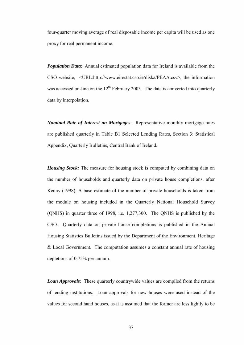
Population Data: Annual estimated population data for Ireland is available from the

CSO website, <URL:http://www.eirestat.cso.ie/diska/PEAA.csv>, the information

was accessed on-line on the 12th February 2003. The data is converted into quarterly

data by interpolation.

Nominal Rate of Interest on Mortgages: Representative monthly mortgage rates

are published quarterly in Table B1 Selected Lending Rates, Section 3: Statistical

Appendix, Quarterly Bulletins, Central Bank of Ireland.

Housing Stock: The measure for housing stock is computed by combining data on

the number of households and quarterly data on private house completions, after

Kenny (1998). A base estimate of the number of private households is taken from

the module on housing included in the Quarterly National Household Survey

(QNHS) in quarter three of 1998, i.e. 1,277,300. The QNHS is published by the

CSO. Quarterly data on private house completions is published in the Annual

Housing Statistics Bulletins issued by the Department of the Environment, Heritage

& Local Government. The computation assumes a constant annual rate of housing

depletions of 0.75% per annum.

Loan Approvals: These quarterly countrywide values are compiled from the returns

of lending institutions. Loan approvals for new houses were used instead of the

values for second hand houses, as it is assumed that the former are less lightly to be

38

tainted by an element of refinancing of existing mortgages. Source: Annual Housing

Statistics Bulletin, issued by the Department of the Environment, Heritage & Local

Government.