Comput Visual Sci (2015) 17:167–183DOI 10.1007/s00791-015-0256-9

Architecture for modeling and simulation of technical systemsalong their lifecycle

Tim Schenk1 · Albert B. Gilg1 · Monika Mühlbauer1 · Roland Rosen1 ·Jan C. Wehrstedt1

Received: 8 July 2015 / Accepted: 16 December 2015 / Published online: 27 January 2016© The Author(s) 2016. This article is published with open access at Springerlink.com

Abstract Modeling and simulation is an established sci-entific and industrial method to support engineers in theirwork in all lifecycle phases—from first concepts or tenderto operation and service—of a technical system. Due to thefact of increasing complexity of such systems, e.g. plants,cyber-physical systems and infrastructures, system simula-tion is rapidly gaining impact. In this paper, a simulationarchitecture is presented and discussed on three differentindustrial applications, which offers a client–server conceptto master the challenges of a lifecycle spanning simulationframework. Looking ahead, open software concepts formod-eling, simulation and optimization will be required to covernew co-simulation techniques and to realize distributed, forexample web-based simulation environments and tools.

1 Introduction

Purpose and objects of computer-based modeling andsimulation have evolved significantly since their first applica-tionsmidof last century. It is nowan established scientific andindustrial analytics and design technology with strong focusand strength to analyze in particular specific physical prod-uct features [1,2]. Numerous powerful tool implementationsare available for use as single stand alone tools and increas-ingly integrated into industrial engineering workflows. Butthe simulation focus continues to address larger systems, notjust components or small products. In the industrial context

Communicated by Gabriel Wittum.

B Tim Schenktim.schenk@siemens.com

1 Siemens AG, Otto-Hahn-Ring 6, 81739 Munich, Germany

this involves tasks of such large and increasingly complexsystems over their whole lifecycle—from first tender to oper-ations and service. Examples range from decision makingduring bidding and conceptual design, detailed engineering,testing and commissioning, as well as optimized runtimeoperations and service [3]. Lumped, so-called 0D simula-tion, and discretized 1D simulation are main technologies toaddress these tasks1 and the presented architectural approachtries to get a grip on them.

The considered fields of application include large processand production plants, power stations and grids, communi-cation networks, different kinds of machines and vehiclesas well as interconnected heterogeneous infrastructure sys-tems.All these systems can be characterized by network-typestructures composed of a multitude of typically heteroge-nous interconnected components. Another important keycharacteristic of such industrial systems are their automa-tion systems for process control by open- and/or closed-loopmechanisms on different levels of detail.

Several commercially available tools, like Matlab Simuli-nk [4], AMESim [5] or Modelica-based Dymola [6], addressthe simulation of such technical systems. They focus oncertain well-confined engineering tasks in specific lifecy-cle phases—mostly detailed engineering—and often tradein computational efficiency (speed and system sizes) againstrestrictions in modeling capabilities and system characteris-tics. Recently, such problem centricmodeling and simulationtools become challenged by further demands. First of all,soaring effort and cost of modeling and tool development arelimiting factors to further progress. Hence, the abundance ofavailable models, model libraries and tool implementationsseems to be an attractive resource and value to reuse concepts.

1 2D and 3D simulations are additionally used especially for detaileddesign and engineering challenges.

123

brought to you by COREView metadata, citation and similar papers at core.ac.uk

provided by Springer - Publisher Connector

168 T. Schenk et al.

But heterogeneity and missing interoperability are criticalobstacles to pursue such approaches. Secondly, the contin-uing progress of computing hardware and network bandwidth opens opportunities to break up complexity bottle-necks. Recent trends, likemulti–core hardware architectures,distributed and cloud computing demand for new system-atic program structures and data flows but are laborious andtricky to be implemented and exploited [7]. Modeling andsimulation architectures need to efficiently support and takeadvantage of these computing resources and paradigm evo-lutions. Thirdly, the involvement of different disciplines anddomains in the system development process further increasessystemheterogeneity and poses additional challenges regard-ing the interplay of multiple disciplines, such as mechanics,electronics, software and communications, during systemevaluations [8,9]. And the system viewpoint is even furtherexpanding to a lifecycle view, which allows for increasingquality and efficiency of system engineering and operation,e.g. system design for reduced lifecycle cost.

The simulation architecture described in this article avoidsthe discussed restrictions of existing tools and faces theupcoming challenges as it allows utilization of a single sim-ulation environment throughout all lifecycle phases and stilloffers the appropriate application support for each task athand by deployment of customized simulation solutions.

The following section introduces three industrial exam-ples of infrastructure and plant systems—a pumping stationfor drinking water, the heat recoverymodule of a power plantand a sewage infrastructure network—which exemplify andillustrate actual simulation issues of real projects. The sectionalso introduces a further key factor to tackle the complexityof modeling and simulation tasks by differentiating betweenthe views of engineers and tool developers.

The subsequent Sect. 3 clusters features of the examplesin Sect. 2 and defines characteristic use cases that cover atypical range of tasks during all lifecycle phases. The usecases reveal the technical requirements, which have to beaddressed by the architectural concept for a modeling andsimulation framework.

Themodeling and simulation frameworkCoSMOS (Com-plex Systems Modeling, Simulation and Optimization)2 isintroduced and outlined in Sect. 4. Its concept as well as thegeneral modular architecture is presented. Two main aspectsof CoSMOS—its focus on a client server architecture and itsembedded simulator—are discussed in detail.

Section 5 exemplifies the applicability of CoSMOS andits specific features along the three industrial examples andtheir individual simulation tasks introduced in Sect. 2.

Together with a short summary, the final section deliversan outlook on some specific issues still open to be solved aswell as future challenges.

2 In house simulation framework of Siemens Corporate Technology.

2 Complexity of system simulation in industrialusage

Industrial simulation is increasingly challenged by systemcomplexity since large systems have to be captured in theirentirety and in many details. Moreover, simulation tool usersand in particular tool developers have different views, i.e.goals and expectations on necessary properties of a simu-lation tool. In the following, three examples of industrialapplications as well as two characteristic views of differentstakeholders are presented to familiarize the reader with theissues faced by industrial system simulations.

2.1 Industrial examples

This selection covers a representative variety of differentapplications covering different phases of a system’s lifecycle.

2.1.1 Pumping station

Water pumping stations enable water transport betweenremote locations. Simulations are used throughout all lifecy-cle phases, from early concept phases to the commissioningphase, plant operations and beyond [10].

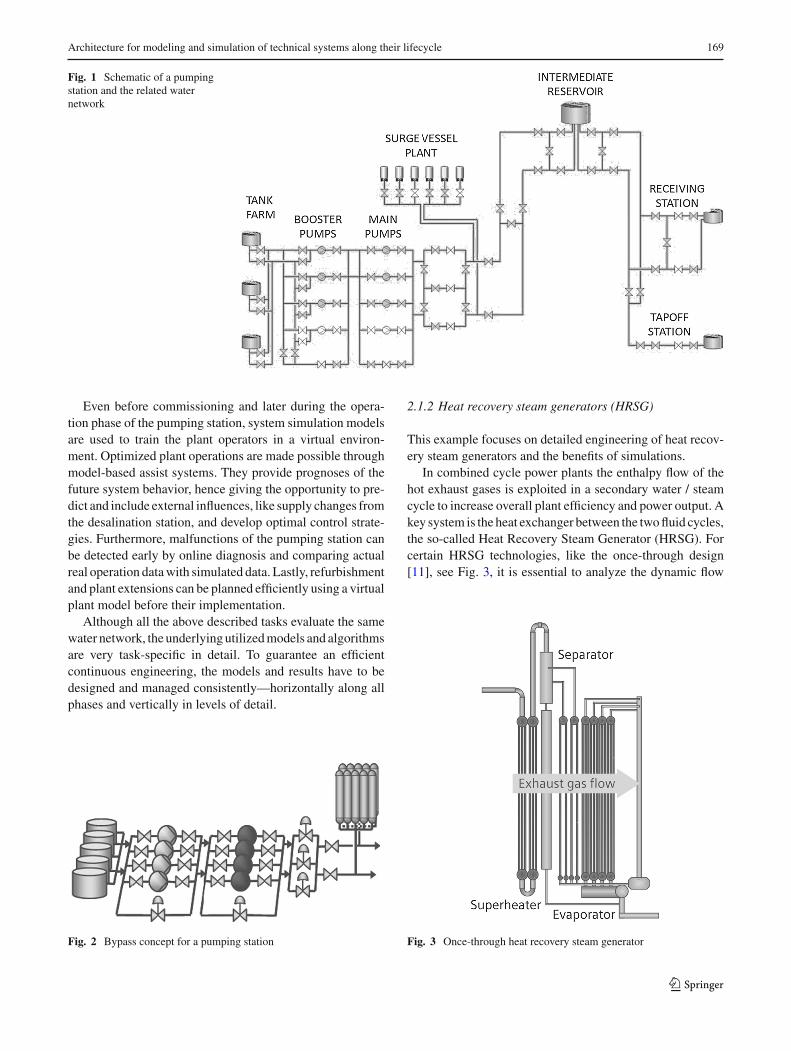
The pumping station presented in this example shall trans-port water from a salt water desalination station througha twin pipeline of 20 kilometer length to an intermedi-ate reservoir situated 500 meters above sea level. Fromthere, the water flows to a receiving and a tap-off stationdriven by gravity, see Fig. 1. The system comprises severalpipelines, tanks with level sensors, valves and pumps to becontrolled.

In the contract bidding and conceptual phase, several basicdesign alternatives are evaluatedwith respect to function, per-formance and cost of required components with the help ofsimulations. In general several parallel booster pumps andthe same number of parallel main pumps are used. Designalternatives to reduce pressure in the pipeline have to be eval-uated, e.g. a shift of the main pumps to a distant location.The tradeoff is to construct an additional pumping stationat a location halfway towards the reservoir with additionalcost and effort, e.g. caused by accessibility problems. In suchearly lifecycle phases only draft models of the componentsand the system layout are available.

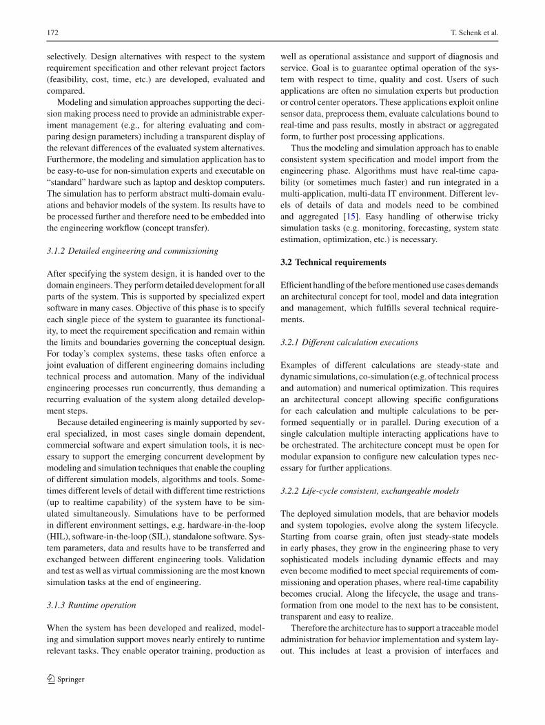
During the engineering phase, modeling and simulationcan support fundamental decisions on specific control andoperation concepts. For example, the so-called bypass con-cept, see Fig. 2, can be configured rather easily, even withoutdetailed engineering expertise. It allows for a partial reflowof the pumped water in order to avoid pump destruction dueto cavitation. Improper operation may even lead to pressureshocks with high risk for damages to the pipelines.

123

Architecture for modeling and simulation of technical systems along their lifecycle 169

Fig. 1 Schematic of a pumpingstation and the related waternetwork

Even before commissioning and later during the opera-tion phase of the pumping station, system simulation modelsare used to train the plant operators in a virtual environ-ment. Optimized plant operations are made possible throughmodel-based assist systems. They provide prognoses of thefuture system behavior, hence giving the opportunity to pre-dict and include external influences, like supply changes fromthe desalination station, and develop optimal control strate-gies. Furthermore, malfunctions of the pumping station canbe detected early by online diagnosis and comparing actualreal operation datawith simulated data. Lastly, refurbishmentand plant extensions can be planned efficiently using a virtualplant model before their implementation.

Although all the above described tasks evaluate the samewater network, the underlyingutilizedmodels and algorithmsare very task-specific in detail. To guarantee an efficientcontinuous engineering, the models and results have to bedesigned and managed consistently—horizontally along allphases and vertically in levels of detail.

Fig. 2 Bypass concept for a pumping station

2.1.2 Heat recovery steam generators (HRSG)

This example focuses on detailed engineering of heat recov-ery steam generators and the benefits of simulations.

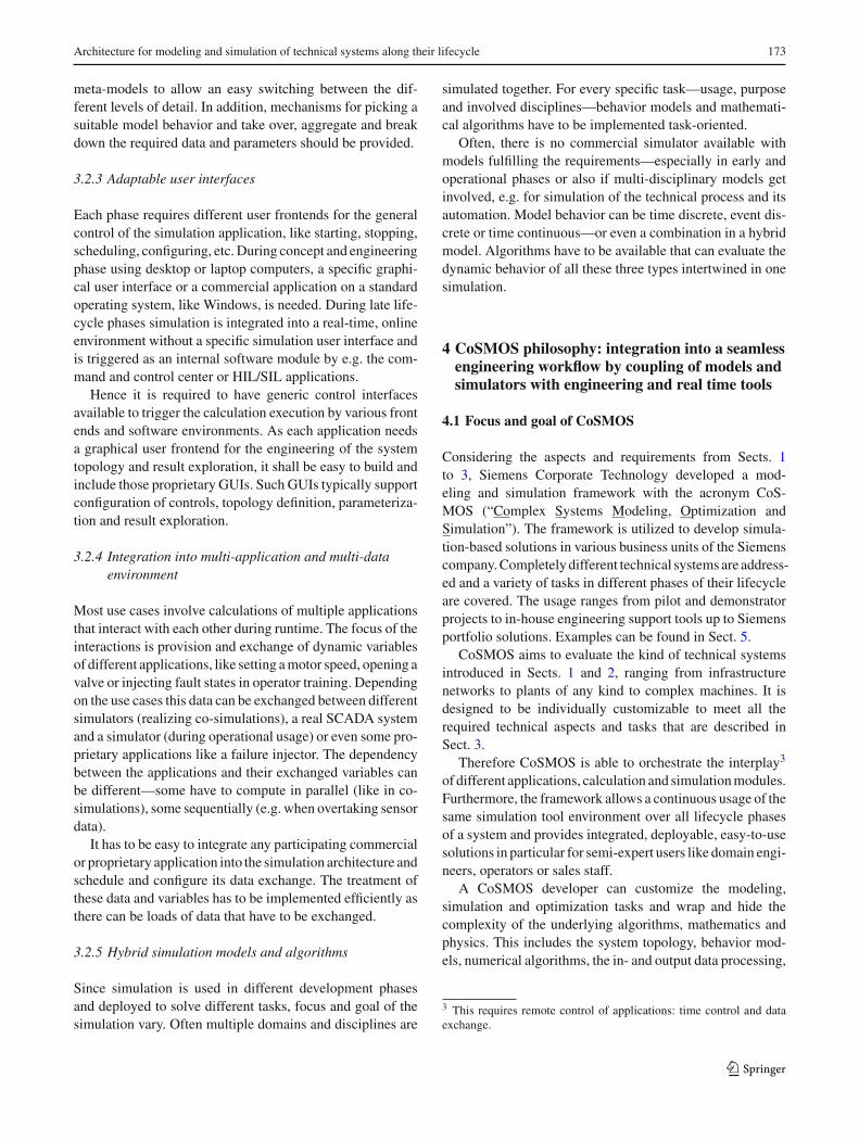
In combined cycle power plants the enthalpy flow of thehot exhaust gases is exploited in a secondary water / steamcycle to increase overall plant efficiency and power output. Akey system is the heat exchanger between the twofluid cycles,the so-called Heat Recovery Steam Generator (HRSG). Forcertain HRSG technologies, like the once-through design[11], see Fig. 3, it is essential to analyze the dynamic flow

Fig. 3 Once-through heat recovery steam generator

123

170 T. Schenk et al.

stability in the design phase in order to ensure a controlledstate at any time during plant operation. For instance, thedesign of valves might need to be adapted to avoid oscilla-tions in pressure and mass flow with high risk of pipe burstsand leakages.

Dynamic analysis of the flow inside such an HRSG isquite tricky: Discretization of the HRSG system leads to alarge number of equations with several thousand degrees offreedom and it contains numerous design parameters suchas number of pipes, their positioning, lengths and diame-ters. Besides, initial values for the flows have to be providedfor calculation. Hence, a manual setup of the model is verytime-consuming and error-prone. This is overcome by anautomatic mapping from previous steady-state simulations,which were performed to fix a primary design of the HRSG.

Finally, beyond the HRSG design tasks, it is of interestto boiler manufacturers and also to OEMs to include theboiler into the overall plant system model as well. For con-trol design and optimization, these plant models are used forearly validation and to define best operation strategies (suchas quick ramp-ups to catch attractive power price windows).To describe the overall plant system, both fluid cycles (gas aswell as water / steam) together with the control system haveto bemodeled in addition to theHRSG. Third party toolsmayprovide suitable libraries for additional components like gasand steam turbines, condensers, pumps or control blocks.

Thus it is attractive to be able to connect several submod-els (HRSG and “periphery”) to provide an overall systemsimulation model. Model integration techniques that allowformulation as a single overall system or co-simulationmeth-ods using independent tools become key issues of industrialsystem simulation.

2.1.3 Sewage network

The third industrial example illustrates operational supportof sewage networks with respect to resource efficiency andenvironmental restrictions enabled by simulation forecastsand optimization algorithms [12,13].

Sewage networks, illustrated in Fig. 4, in cities nowadaysdo not include much automation and control infrastructure.They are mostly run by small local controllers and expe-rienced operators. Main obstacles to include more optimalcontrol equipment are: very small economic benefit for theoperator companies (mostly public services), despite of pub-lic and environmental benefits, the uncertainties to predictsystem inflow profiles from rain and sewage producers anddifficulties to understand handling alternatives and their longtime impact in such a sewage network.

However, the increasing occurrence of more and heavierdownpours, the fact of low city budgets for infrastructureinvestments and the increasing environmental awareness of

Sewer 1

Inflow 3

SewagePlant

Sewer 2 Sewer 3

Inflow 1

Valve 1

Valve 3

Inflow 2

Valve 2

StormwaterTank 1

StormwaterTank 2

Rainstoragesewer

Sewer 4

Valve 4

Discharge

Discharge

Discharge

Control

Control

Control Control

Fig. 4 Functional scheme of a small sewage network

123

Architecture for modeling and simulation of technical systems along their lifecycle 171

the public call for better operation controls. Cheaper sen-sor technology and availability of wireless communicationinfrastructure in combination with efficient simulation mod-els are cornerstones to successfully develop and provideIT-based operational support. This enables solutions for dif-ferent tasks: Network monitoring of actual and predictionof future network states; forecasting of consequences fordifferent selected control strategies; automatically generatedsuggestions for changes of valve and pump settings for dif-ferent operation points like for example rain events. Evena 24/7 fully automated, optimal control of a sewer networkmay become possible.

Some of these tasks can use offline simulation runs, e.g.concept studies helping in investment decisions or in review-ing the necessity of control decisions during past events. Thissimulation requires a 1D simulation of wastewater flow, pres-surized and open channel flow, through the network. Butmost of the tasks need online simulation capability in thecontrol center during network operation and will be directlyconnected to the Supervisory Control and Data Acquisition(SCADA) system to access actual sensor data (e.g. flow val-ues, filling levels, valve positions, rain data).

In particular, tasks performed during operation should beable to run in parallel or in a specified sequential order. Eachof these tasks may be configured differently regarding whenand how it is executed. For example, the network monitoringshall run every 15 minutes, but a forecast or an optimiza-tion for an upcoming downpour shall be triggered by theoperator—without stopping the monitoring.

2.2 “Bi-view” engineer vs. IT approach

Besides the complexity of the applications themselves, sys-tem simulation environments have to fulfill very differentrequirements of their stakeholders. There are two maingroups of stakeholders.

First of all there are users, i.e. engineers, who have toperform specific tasks in dedicated system lifecycle phases.They require one or if not avoidable several simulation toolsthat hopefully support perfectly. Considering for example thesetup of a component-based simulation model, an engineer’swork typically comprises the instantiation of all components,stemming eventually from different component libraries anddefining their interconnections. Furthermore, the setting ofparameters, like geometric dimensions, and of initial compo-nent states and boundary conditions, such as the initial fillinglevel of tanks, needs to be performed. After specifying sim-ulation run configurations, like simulated time intervals anda preferably small set of solver settings, simulation runs areexecuted and results will be evaluated during and/or after thesimulation run via graphical viewers. The engineer requests(semi-)automatic support by the tool for his tasks wheneverpossible to reduce the work load. This ranges from automatic

model generation, help in setting a most suitable simulationconfiguration for specific tasks up to scenario managementand result interpretation.

This engineer’s focus is not on underlying tool conceptssuch as algorithms and implementation, software service andupgrade concepts. These are in focus of the other group ofstakeholders, the tool vendors and developers and their ITcentered viewpoint. Their target is to cover asmuch customerdemand as necessary while keeping cost of implementationand service as low as possible. One key goal is to enableall the functionality for each type of simulation task in auser-friendly way. This comprises, among other things, thedevelopment and supply of component libraries in variouslevels of detail, as well as advanced solving algorithms forlarge systems of equations with time continuous as wellas time discrete variables. Additionally, further demandsregarding the time management can arise, like real-timerequirements.

These demands resulted in a vast landscape of task andapplication specific simulations tools. Main challenges arereduction of modeling cost by reuse of existing models andinteroperability of dedicated tools. Promising techniques likeco-simulation via flexible interface descriptions are becom-ing established (e.g. the Functional Mockup Interface [14]).

3 Use cases and their technical requirements

Reviewing the industrial examples and both viewpoints fromSect. 2, this section defines characteristic use cases and theconsequent technical requirements for themodeling and sim-ulation architecture.

3.1 Use cases

The following three use cases address the main phases of asystem lifecycle with quite different simulation objectives.Many more use cases could be defined during designing,developing or operating technical systems, products andplants. Yet, this selection is quite generic so that most otheruse cases should be minor modifications or a combination ofthe three ones presented here.

3.1.1 Decision making in early planning and conceptualdesign

Developing a new technical system starts with a conceptualplanning phase. The goal is to create the layout of the system,outline its main boundaries, content and parameters. Thisphase is characterized by abstract or at most half-detailedtechnical system specifications. Most of the tasks are per-formed by a small team of system designers. Expertise andfeedback from customers and domain experts is collected

123

172 T. Schenk et al.

selectively. Design alternatives with respect to the systemrequirement specification and other relevant project factors(feasibility, cost, time, etc.) are developed, evaluated andcompared.

Modeling and simulation approaches supporting the deci-sion making process need to provide an administrable exper-iment management (e.g., for altering evaluating and com-paring design parameters) including a transparent display ofthe relevant differences of the evaluated system alternatives.Furthermore, the modeling and simulation application has tobe easy-to-use for non-simulation experts and executable on“standard” hardware such as laptop and desktop computers.The simulation has to perform abstract multi-domain evalu-ations and behavior models of the system. Its results have tobe processed further and therefore need to be embedded intothe engineering workflow (concept transfer).

3.1.2 Detailed engineering and commissioning

After specifying the system design, it is handed over to thedomain engineers. They performdetailed development for allparts of the system. This is supported by specialized expertsoftware in many cases. Objective of this phase is to specifyeach single piece of the system to guarantee its functional-ity, to meet the requirement specification and remain withinthe limits and boundaries governing the conceptual design.For today’s complex systems, these tasks often enforce ajoint evaluation of different engineering domains includingtechnical process and automation. Many of the individualengineering processes run concurrently, thus demanding arecurring evaluation of the system along detailed develop-ment steps.

Because detailed engineering is mainly supported by sev-eral specialized, in most cases single domain dependent,commercial software and expert simulation tools, it is nec-essary to support the emerging concurrent development bymodeling and simulation techniques that enable the couplingof different simulation models, algorithms and tools. Some-times different levels of detail with different time restrictions(up to realtime capability) of the system have to be sim-ulated simultaneously. Simulations have to be performedin different environment settings, e.g. hardware-in-the-loop(HIL), software-in-the-loop (SIL), standalone software. Sys-tem parameters, data and results have to be transferred andexchanged between different engineering tools. Validationand test as well as virtual commissioning are the most knownsimulation tasks at the end of engineering.

3.1.3 Runtime operation

When the system has been developed and realized, model-ing and simulation support moves nearly entirely to runtimerelevant tasks. They enable operator training, production as

well as operational assistance and support of diagnosis andservice. Goal is to guarantee optimal operation of the sys-tem with respect to time, quality and cost. Users of suchapplications are often no simulation experts but productionor control center operators. These applications exploit onlinesensor data, preprocess them, evaluate calculations bound toreal-time and pass results, mostly in abstract or aggregatedform, to further post processing applications.

Thus the modeling and simulation approach has to enableconsistent system specification and model import from theengineering phase. Algorithms must have real-time capa-bility (or sometimes much faster) and run integrated in amulti-application, multi-data IT environment. Different lev-els of details of data and models need to be combinedand aggregated [15]. Easy handling of otherwise trickysimulation tasks (e.g. monitoring, forecasting, system stateestimation, optimization, etc.) is necessary.

3.2 Technical requirements

Efficient handlingof the beforementioneduse cases demandsan architectural concept for tool, model and data integrationand management, which fulfills several technical require-ments.

3.2.1 Different calculation executions

Examples of different calculations are steady-state anddynamic simulations, co-simulation (e.g. of technical processand automation) and numerical optimization. This requiresan architectural concept allowing specific configurationsfor each calculation and multiple calculations to be per-formed sequentially or in parallel. During execution of asingle calculation multiple interacting applications have tobe orchestrated. The architecture concept must be open formodular expansion to configure new calculation types nec-essary for further applications.

3.2.2 Life-cycle consistent, exchangeable models

The deployed simulation models, that are behavior modelsand system topologies, evolve along the system lifecycle.Starting from coarse grain, often just steady-state modelsin early phases, they grow in the engineering phase to verysophisticated models including dynamic effects and mayeven become modified to meet special requirements of com-missioning and operation phases, where real-time capabilitybecomes crucial. Along the lifecycle, the usage and trans-formation from one model to the next has to be consistent,transparent and easy to realize.

Therefore the architecture has to support a traceablemodeladministration for behavior implementation and system lay-out. This includes at least a provision of interfaces and

123

Architecture for modeling and simulation of technical systems along their lifecycle 173

meta-models to allow an easy switching between the dif-ferent levels of detail. In addition, mechanisms for picking asuitable model behavior and take over, aggregate and breakdown the required data and parameters should be provided.

3.2.3 Adaptable user interfaces

Each phase requires different user frontends for the generalcontrol of the simulation application, like starting, stopping,scheduling, configuring, etc.During concept and engineeringphase using desktop or laptop computers, a specific graphi-cal user interface or a commercial application on a standardoperating system, like Windows, is needed. During late life-cycle phases simulation is integrated into a real-time, onlineenvironment without a specific simulation user interface andis triggered as an internal software module by e.g. the com-mand and control center or HIL/SIL applications.

Hence it is required to have generic control interfacesavailable to trigger the calculation execution by various frontends and software environments. As each application needsa graphical user frontend for the engineering of the systemtopology and result exploration, it shall be easy to build andinclude those proprietary GUIs. Such GUIs typically supportconfiguration of controls, topology definition, parameteriza-tion and result exploration.

3.2.4 Integration into multi-application and multi-dataenvironment

Most use cases involve calculations of multiple applicationsthat interact with each other during runtime. The focus of theinteractions is provision and exchange of dynamic variablesof different applications, like setting amotor speed, opening avalve or injecting fault states in operator training. Dependingon the use cases this data can be exchanged between differentsimulators (realizing co-simulations), a real SCADA systemand a simulator (during operational usage) or even some pro-prietary applications like a failure injector. The dependencybetween the applications and their exchanged variables canbe different—some have to compute in parallel (like in co-simulations), some sequentially (e.g. when overtaking sensordata).

It has to be easy to integrate any participating commercialor proprietary application into the simulation architecture andschedule and configure its data exchange. The treatment ofthese data and variables has to be implemented efficiently asthere can be loads of data that have to be exchanged.

3.2.5 Hybrid simulation models and algorithms

Since simulation is used in different development phasesand deployed to solve different tasks, focus and goal of thesimulation vary. Often multiple domains and disciplines are

simulated together. For every specific task—usage, purposeand involved disciplines—behavior models and mathemati-cal algorithms have to be implemented task-oriented.

Often, there is no commercial simulator available withmodels fulfilling the requirements—especially in early andoperational phases or also if multi-disciplinary models getinvolved, e.g. for simulation of the technical process and itsautomation. Model behavior can be time discrete, event dis-crete or time continuous—or even a combination in a hybridmodel. Algorithms have to be available that can evaluate thedynamic behavior of all these three types intertwined in onesimulation.

4 CoSMOS philosophy: integration into a seamlessengineering workflow by coupling of models andsimulators with engineering and real time tools

4.1 Focus and goal of CoSMOS

Considering the aspects and requirements from Sects. 1to 3, Siemens Corporate Technology developed a mod-eling and simulation framework with the acronym CoS-MOS (“Complex Systems Modeling, Optimization andSimulation”). The framework is utilized to develop simula-tion-based solutions in various business units of the Siemenscompany.Completely different technical systems are address-ed and a variety of tasks in different phases of their lifecycleare covered. The usage ranges from pilot and demonstratorprojects to in-house engineering support tools up to Siemensportfolio solutions. Examples can be found in Sect. 5.

CoSMOS aims to evaluate the kind of technical systemsintroduced in Sects. 1 and 2, ranging from infrastructurenetworks to plants of any kind to complex machines. It isdesigned to be individually customizable to meet all therequired technical aspects and tasks that are described inSect. 3.

Therefore CoSMOS is able to orchestrate the interplay3

of different applications, calculation and simulationmodules.Furthermore, the framework allows a continuous usage of thesame simulation tool environment over all lifecycle phasesof a system and provides integrated, deployable, easy-to-usesolutions in particular for semi-expert users like domain engi-neers, operators or sales staff.

A CoSMOS developer can customize the modeling,simulation and optimization tasks and wrap and hide thecomplexity of the underlying algorithms, mathematics andphysics. This includes the system topology, behavior mod-els, numerical algorithms, the in- and output data processing,

3 This requires remote control of applications: time control and dataexchange.

123

174 T. Schenk et al.

Simulator

Library Metamodel

System Topology

BaseClient

Job Configuration

Control API

Control System(JobManager &

Server)

Uses

Dynamic Exchange

ReadsReads

CommandsDerives

(Generic) Interfaces

CalculationProcessing

CoSMOS Core

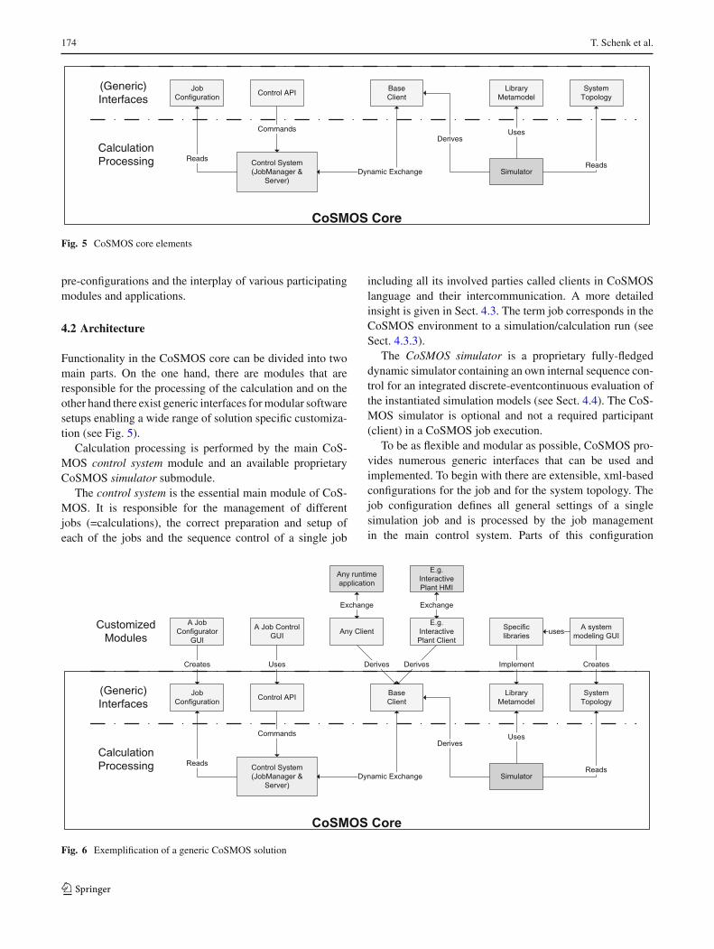
Fig. 5 CoSMOS core elements

pre-configurations and the interplay of various participatingmodules and applications.

4.2 Architecture

Functionality in the CoSMOS core can be divided into twomain parts. On the one hand, there are modules that areresponsible for the processing of the calculation and on theother hand there exist generic interfaces formodular softwaresetups enabling a wide range of solution specific customiza-tion (see Fig. 5).

Calculation processing is performed by the main CoS-MOS control system module and an available proprietaryCoSMOS simulator submodule.

The control system is the essential main module of CoS-MOS. It is responsible for the management of differentjobs (=calculations), the correct preparation and setup ofeach of the jobs and the sequence control of a single job

including all its involved parties called clients in CoSMOSlanguage and their intercommunication. A more detailedinsight is given in Sect. 4.3. The term job corresponds in theCoSMOS environment to a simulation/calculation run (seeSect. 4.3.3).

The CoSMOS simulator is a proprietary fully-fledgeddynamic simulator containing an own internal sequence con-trol for an integrated discrete-eventcontinuous evaluation ofthe instantiated simulation models (see Sect. 4.4). The CoS-MOS simulator is optional and not a required participant(client) in a CoSMOS job execution.

To be as flexible and modular as possible, CoSMOS pro-vides numerous generic interfaces that can be used andimplemented. To begin with there are extensible, xml-basedconfigurations for the job and for the system topology. Thejob configuration defines all general settings of a singlesimulation job and is processed by the job managementin the main control system. Parts of this configuration

Specific libraries

Simulator

A system modeling GUI

A Job Configurator

GUI

A Job Control GUI

E.g. Interactive Plant HMI

Any runtime application

E.g. Interactive Plant Client

Any Client uses

Library Metamodel

System Topology

BaseClient

Job Configuration Control API

Control System(JobManager &

Server)

ExchangeExchange

Derives Implement

Uses

DerivesUsesCreates Creates

Dynamic Exchange

ReadsReads

CommandsDerives

(Generic) Interfaces

CustomizedModules

CalculationProcessing

CoSMOS Core

Fig. 6 Exemplification of a generic CoSMOS solution

123

Architecture for modeling and simulation of technical systems along their lifecycle 175

are the time control settings, the specific configuration ofeach participating client and the management of results.The system topology is stored separately in another con-figuration file following the component-based principlesstated in Sect. 4.1 consisting of components, parametersand connections. This configuration can contain severaldiffering versions of the same system depending on thepurpose of further processing. For example, there is atleast a version for the general layout containing compo-nents and their graphical representation. Each participant(client) that processes proprietary system topology infor-mation can add a specific version containing the clientspecific information. For example, the proprietary CoS-MOS simulator adds a version containing simulation relevantinformation, like interconnection types and values of para-meters.

Besides these two configurations, CoSMOS providesbase classes and meta models that can be implementedto extend and add functionality. There is a base client tobe implemented by any application that wants to partic-ipate in a simulation run and therefore becomes a client(see Sect. 4.3.1). To be able to manage various jobsand control the execution of each single job, there isan API control interface that provides functionality forcreating, loading, starting, stopping, etc. of jobs. Pro-viding the CoSMOS simulator with own libraries con-taining behavior models can be done by implementingthe library meta model (see Sect. 4.4), as it is availablein most commercial simulators, like the ones stated inSect. 4.1.

For exemplification, a usage and implementation ina classical programming language like C++ or C# ofall the interfaces is shown in Fig. 6 by a generic cus-tomization. This way a complete application serving aspecific purpose can be built—also called CoSMOS solu-tion.

The presented architecture supports implicitly a genericengineering workflow. Depending on the solution, specificmodules required for modeling, configuration, control andthe runtime participants (clients) can be customized, inte-grated and configured.

The CoSMOS control system can be operated with dif-ferent specific GUIs or even completely hidden behind anexisting HMI system like PCS 7 OS [16] for use in a controlcenter and automatically executed by it. Stored job configura-tions can be reused and extended, e.g. predefined offline andloaded during the operation. And participating applicationscan be flexibly added and removed by loading and unloadingtheir clients, e.g. to communicate between a process simu-lator and a emulated programmable logic control (PLC) ina Software-in-the-loop test environment or to write simu-lation data to MS Office applications when doing conceptdesign studies. System topologies that were created in a

former development phase can easily be reused in later eval-uation by e.g. exchanging the library with a more detailedone.

4.3 Control system

4.3.1 Client–server concept

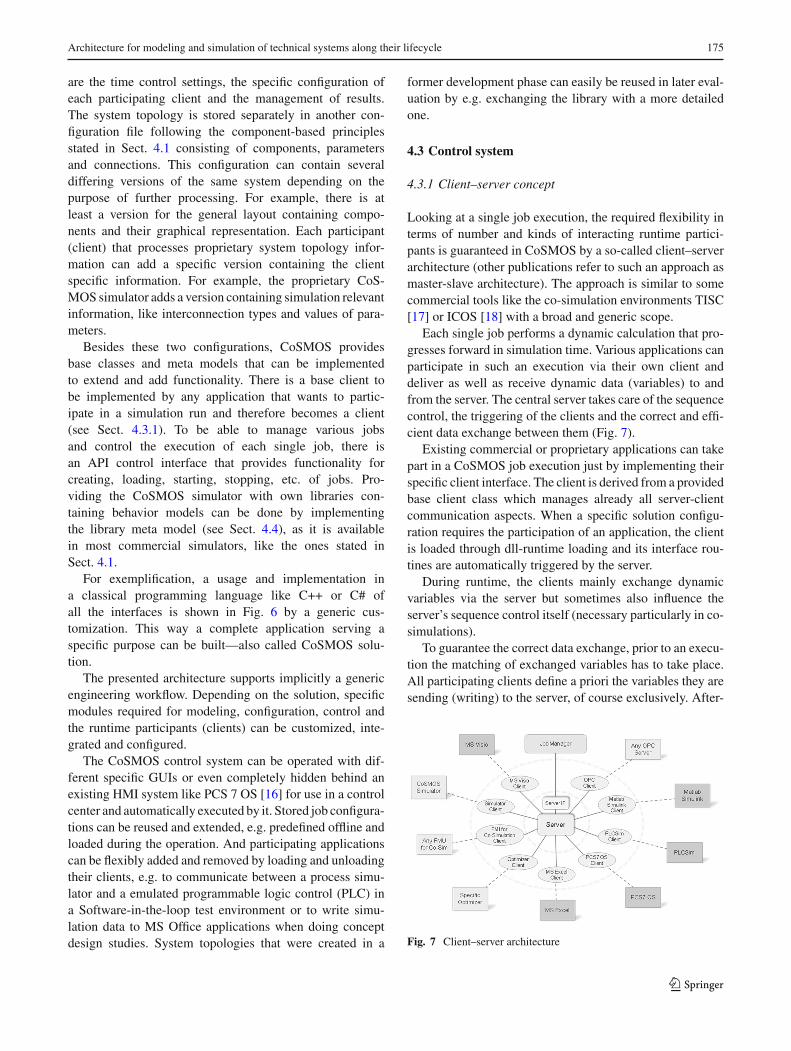
Looking at a single job execution, the required flexibility interms of number and kinds of interacting runtime partici-pants is guaranteed in CoSMOS by a so-called client–serverarchitecture (other publications refer to such an approach asmaster-slave architecture). The approach is similar to somecommercial tools like the co-simulation environments TISC[17] or ICOS [18] with a broad and generic scope.

Each single job performs a dynamic calculation that pro-gresses forward in simulation time. Various applications canparticipate in such an execution via their own client anddeliver as well as receive dynamic data (variables) to andfrom the server. The central server takes care of the sequencecontrol, the triggering of the clients and the correct and effi-cient data exchange between them (Fig. 7).

Existing commercial or proprietary applications can takepart in a CoSMOS job execution just by implementing theirspecific client interface. The client is derived from a providedbase client class which manages already all server-clientcommunication aspects. When a specific solution configu-ration requires the participation of an application, the clientis loaded through dll-runtime loading and its interface rou-tines are automatically triggered by the server.

During runtime, the clients mainly exchange dynamicvariables via the server but sometimes also influence theserver’s sequence control itself (necessary particularly in co-simulations).

To guarantee the correct data exchange, prior to an execu-tion the matching of exchanged variables has to take place.All participating clients define a priori the variables they aresending (writing) to the server, of course exclusively. After-

Fig. 7 Client–server architecture

123

176 T. Schenk et al.

Fig. 8 Data exchange from and to clients

wards, the variables each client wants to obtain (read) arelinked to one variable in the list of all available variables—either automatically or defined manually by the user. Thereare available automatic matching routines like pure namematching, but individual matchings can be implemented,added and used as well. During a job execution, the servertriggers each client at specific time points depending on theclient configuration (read variables, do calculations, writevariables, see Fig. 8).

The trigger time points can differ from client to client,depending on the simulation task and the purpose of eachclient. When more than one client has to be called at a trig-ger point, the clients are per default evaluated in parallel.E.g. two simulator clients, running in a co-simulation, wouldprobably have the same trigger points, while a client thatupdates only a visualization in e.g. MS Visio or PCS 7 OS(Siemens control station HMI) can have longer time stepsbetween its trigger points than the simulators. Usually, trig-ger points are defined before the actual job execution, butdetection of certain events during a simulation can lead toadditional trigger points which will be added on the fly.

4.3.2 Scheduling of clients

To execute dynamic simulations, the server control pro-gresses forward in time and calls the participating clients attheir trigger time points as stated above. Naturally, all partic-ipating clients can simulate dynamic behavior with the sameclock—or in other words can integrate in each step from theactual trigger time point to the next. But often enough, theydo have an own, different internal clock (e.g. performing aforecast) or just perform a proprietary sort of data processing

or similar. Examples for that are the visualization of sim-ulated variables in an individual graphical user front-end,preprocessing of data for the further usage in the simulatorand even optimizations and the calculation of KPIs at a spe-cific point in time. As the architecture of CoSMOS is basedon the modular client–server concept, all those functionali-ties are not implemented as add-on to a simulator itself, butare realized as capabilities of the clients that exchange theirdata via the server. This way they can be reused in all kindsof CoSMOS solutions with all kinds of simulators.

As stated above, clients with a common trigger time pointare called by default in parallel to do their calculation. Ifrequired, it is also possible to schedule the calls of “sta-tionary” and “dynamic” clients at trigger time points in thecorrect order. E.g., when for a specific task the simulator isin need of data that has to be preprocessed in each step, theclient performing the preprocessing is scheduled before thesimulator. This way the data required from the simulator isalready present in the server. Another example is the needfor visualization during a simulation execution. The visual-ization client naturally should show the actual values of thevariables. Therefore it has to be scheduled after the simulatorto get the newly calculated values (see Fig. 9).

4.3.3 Job concept

So far the explained concepts deal with the execution of sin-gle simulation runs that can be executed immediately and runas fast as possible. As in the industrial examples and use casesalready stated, it can also be necessary to schedule simulationruns, couple them to real-time or even perform multiple sim-ulation executions in parallel or in specific orders—primarily

123

Architecture for modeling and simulation of technical systems along their lifecycle 177

Fig. 9 Example of client scheduling

these requirements appear in environments like experimentand test management and operational support. In CoSMOS,this possibility has been implemented with the job concept.

The concept defines each simulation run as a single job.One job contains a complete client–server setup as describedin Sects. 4.3.1 and 4.3.2. The job concept adds to theconfiguration of a single run—consisting of the setup andconfigurations of clients and some basic run settings—anextensive time control configuration. Each job can be sched-uled with a start time in real time and synchronized withreal-time at specified synchronization time points.Moreover,the job can relate its time behavior to real-time labels (virtualreal-time).

Complex setups like real-time clocked co-simulations canbe performed (see Fig. 10). Simulation steps can be executedperiodically in the real-time environment of an operationalsupport system.

To correctly handle jobs, a job manager is implementedin CoSMOS. Apart from managing only a single job, the jobmanager can be fed with multiple jobs and configured how todeal with them. If the number of processing units allows it,jobs that overlap in their execution time interval will be exe-cuted in parallel on different processors. If no free processoris available or it is not intended to execute jobs in parallel,the jobs are executed due to their predefined priorities. A jobof minor priority then has to be stopped for later resumptionand a job of higher priority is executed first instead.

4.4 Simulator

Besides the possibility to integrate any (commercial) sim-ulator via the client concept, a proprietary simulator isalso available in CoSMOS. As every other participant it isimplemented as a CoSMOS client and exchanges dynamic

variables with the server. This simulator performs efficientdynamic simulations.

Themodel concept followedby the simulator is component-based as described in Sect. 4.1. This means that the behaviorof the whole system results out of the behavior of the instan-tiation of the types of components and their interconnectionbetween each other.

Thus the CoSMOS simulator builds its internal systemsimulation model by processing its respective version of thesystem topology configuration (Sect. 4.2) and subsequentlyinstantiating and parameterizing every component and con-nection of the topology from the available model libraries.At last the ports of the component instances are connectedappropriately to ensure the physical, logical and signal flowsbetween the components.

The sequence control of the CoSMOS simulator copeswith event-discrete, time-discrete and continuous models atthe same time and furthermore enables differential-algebraicequations (DAEs) in the continuous modeling, which aresolved in one complete equation system altogether by spe-cial, time efficient DAE-solvers for networked systems ina mathematical sense [19]. This allows also the solution ofdiscretized partial differential equations. The sequence con-trol follows a natural hierarchy, based on the principle of theautomation pyramid (see Fig. 11): The time discrete evalu-ation interrupts the continuous integration for exchange ofinformation, whereas events trigger a specific evaluation inthe time discrete and subsequently in the continuous model.

Technological processes aremostlymodeled continuouslybeing a synonym for a description by (partial) differentialalgebraic equation systems, consisting of equations and inde-pendent variables. These are evaluated on a continuous timelevel and require special numerical solvers. Every compo-nent modeling continuous behavior can define independentvariables (DoFs—degrees of freedom) and implement the

123

178 T. Schenk et al.

Fig. 10 Real-time synchronized simulation

equations (algebraic and/or differential) in the function callsprovided by the meta-model. The CoSMOS simulator col-lects all DoFs and equations of all instantiated componentsto build one system of equations and a vector of DoFs. Fig-ure 12 illustrates this approach with a pipe connecting totanks. The numerical integration of the DoFs describes thebehavior of the continuous part of the modeled system. Asspecial types of equations require special numerical solvers,CoSMOS offers the possibility to integrate different numer-ical solver.

In time and event discrete modeling, usually certainstates are defined, which are evaluated either every fixeddiscrete sample rate or when events occur. Thus automa-tion and control logic behavior is typically modeled timediscrete and event-discrete modeling is used mainly in

Fig. 11 Three different models and their relation

event-driven domains, like traffic, transport and logisticssystems.

When implementing time discrete behavior, a componentdefines its states and realizes their calculation in the func-tion calls provided by the meta-model. The internal statesare calculated mostly out of the input signals of the compo-nents and afterwards the output signals of components are set.The simulator stops the continuous integration every precon-figured sample time point (mostly equidistantly) and startsthe algorithm for the discrete system—realized by the fol-lowing empty loop procedure: All discrete components areevaluated in a random order to avoid deadlocks because ofperiodic cycles. In doing so for every component, the internalstates and output values are calculated according to the actualinput values. This procedure will be repeated as long as anyinternal state of the whole system changes. If the fixed pointis reached within a prescribed time, the continuous simula-tion will proceed to calculate till the next sample time point.Otherwise, the system does not converge mostly due to ille-gitimate loops by wrongly connected components.

In the case of event-discrete behavior, the time point atwhich the continuous integration is stopped and the statesare calculated is triggered by events. Every component cangenerate and queue events. Each event is configured with thetime when it fires, the dispatcher and the recipient compo-nent of the event. The simulator contains therefore an eventmanager, which collects all created events, queues them inthe correct order and executes each one at its specific timepoint.

As theCoSMOSsimulator supports all three types ofmod-eling and the combined processing, there is no need to switchto another simulator when it seemsmore appropriate or moreefficient to model parts of the continuous systems in a timeor event discrete way or vice versa.

123

Architecture for modeling and simulation of technical systems along their lifecycle 179

Fig. 12 Instantiated, connected components lead to the system of equations

5 Exemplification

In the following, the industrial examples of Sect. 2 will beconsidered regarding their implementation in the simulationenvironment CoSMOS as it is described in Sect. 4.

5.1 Pumping station

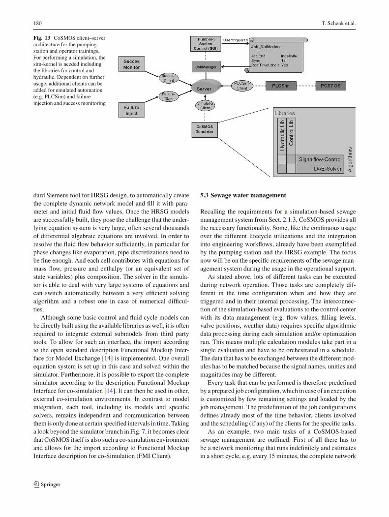
For the simulation of the pumping station, which is targetedby several development phases addressed in the differentuse cases of Sect. 3, a very flexible software system isneeded: In an early conceptual phase, the latter consists of anengineering GUI, a CoSMOS simulator handling a networkof components from hydraulic and automation libraries bynumerical solvers for mixed discrete and continuous systemsand a result evaluation. Later on, for virtual commission-ing, an emulated PLC, such as SIMATIC S7 PLCSim [20],SIMATIC WinAC RTX [21] or SIMIT Emulation Platform[22], is added to the architecture to analyze real PLC soft-ware in the loop. The automation part of the system isthen no longer modeled in the CoSMOS simulator, wherethe automation part of the model needs to be removed, butprovided by SIMATIC PCS 7 OS, which is connected tothe emulated PLC using standard SIMATIC technologies.Finally, for operator training, additional tools like successcontrol and failure injection are added to the client–serverarchitecture, see Fig. 13.

To obtain the network model of components for the simu-lator (CoSMOS Simulator), two approaches exist. First, the

engineer could build the model manually in the engineeringGUI by drag&drop, connection and individual parameteri-zation of all components needed from the libraries. Second,less error-prone and more efficiently, the model setup canbe done semi-automatically by model generation from plantengineering tools like COMOS, which contain engineer-ing artifacts like the pipe and instrumentation diagram aswell as technical data of the components like character-istic curves, geometries etc. Only additional informationlike initial values has then to be added by the engineerto get a complete description of the simulation model[10].

Having defined the individual settings of all clients, e.g.solver selection and tolerances for the simulator, the detailsof the server communication and data exchange need to beset, e.g. the length of communication time interval as well asthe matching of exchange variables between different clientsvia matching table. These matching have to be performedfor any involved client and modified if clients are added orremoved.

5.2 Heat recovery steam generators (HRSGs)

Regarding the dynamic simulations of HRSGs introduced inSect. 2.1.2, the simulator in CoSMOS incorporates dedicatedlibraries for boilers. The HRSG models can be assembledby simple drag-and-drop from these libraries. In order toallow for a seamless workflow, however, it is also possibleto import the steady-state solution of KrawalTM [23], a stan-

123

180 T. Schenk et al.

Fig. 13 CoSMOS client–serverarchitecture for the pumpingstation and operator trainings.For performing a simulation, thesim-kernel is needed includingthe libraries for control andhydraulic. Dependent on furtherusage, additional clients can beadded for emulated automation(e.g. PLCSim) and failureinjection and success monitoring

dard Siemens tool for HRSG design, to automatically createthe complete dynamic network model and fill it with para-meter and initial fluid flow values. Once the HRSG modelsare successfully built, they pose the challenge that the under-lying equation system is very large, often several thousandsof differential algebraic equations are involved. In order toresolve the fluid flow behavior sufficiently, in particular forphase changes like evaporation, pipe discretizations need tobe fine enough. And each cell contributes with equations formass flow, pressure and enthalpy (or an equivalent set ofstate variables) plus composition. The solver in the simula-tor is able to deal with very large systems of equations andcan switch automatically between a very efficient solvingalgorithm and a robust one in case of numerical difficul-ties.

Although some basic control and fluid cycle models canbe directly built using the available libraries aswell, it is oftenrequired to integrate external submodels from third partytools. To allow for such an interface, the import accordingto the open standard description Functional Mockup Inter-face for Model Exchange [14] is implemented. One overallequation system is set up in this case and solved within thesimulator. Furthermore, it is possible to export the completesimulator according to the description Functional MockupInterface for co-simulation [14]. It can then be used in other,external co-simulation environments. In contrast to modelintegration, each tool, including its models and specificsolvers, remains independent and communication betweenthem is only done at certain specified intervals in time. Takinga look beyond the simulator branch in Fig. 7, it becomes clearthat CoSMOS itself is also such a co-simulation environmentand allows for the import according to Functional MockupInterface description for co-Simulation (FMI Client).

5.3 Sewage water management

Recalling the requirements for a simulation-based sewagemanagement system from Sect. 2.1.3, CoSMOS provides allthe necessary functionality. Some, like the continuous usageover the different lifecycle utilizations and the integrationinto engineering workflows, already have been exemplifiedby the pumping station and the HRSG example. The focusnow will be on the specific requirements of the sewage man-agement system during the usage in the operational support.

As stated above, lots of different tasks can be executedduring network operation. Those tasks are completely dif-ferent in the time configuration when and how they aretriggered and in their internal processing. The interconnec-tion of the simulation-based evaluations to the control centerwith its data management (e.g. flow values, filling levels,valve positions, weather data) requires specific algorithmicdata processing during each simulation and/or optimizationrun. This means multiple calculation modules take part in asingle evaluation and have to be orchestrated in a schedule.The data that has to be exchanged between the different mod-ules has to be matched because the signal names, unities andmagnitudes may be different.

Every task that can be performed is therefore predefinedby a prepared job configuration,which in case of an executionis customized by few remaining settings and loaded by thejob management. The predefinition of the job configurationsdefines already most of the time behavior, clients involvedand the scheduling (if any) of the clients for the specific tasks.

As an example, two main tasks of a CoSMOS-basedsewage management are outlined: First of all there has tobe a network monitoring that runs indefinitely and estimatesin a short cycle, e.g. every 15 minutes, the complete network

123

Architecture for modeling and simulation of technical systems along their lifecycle 181

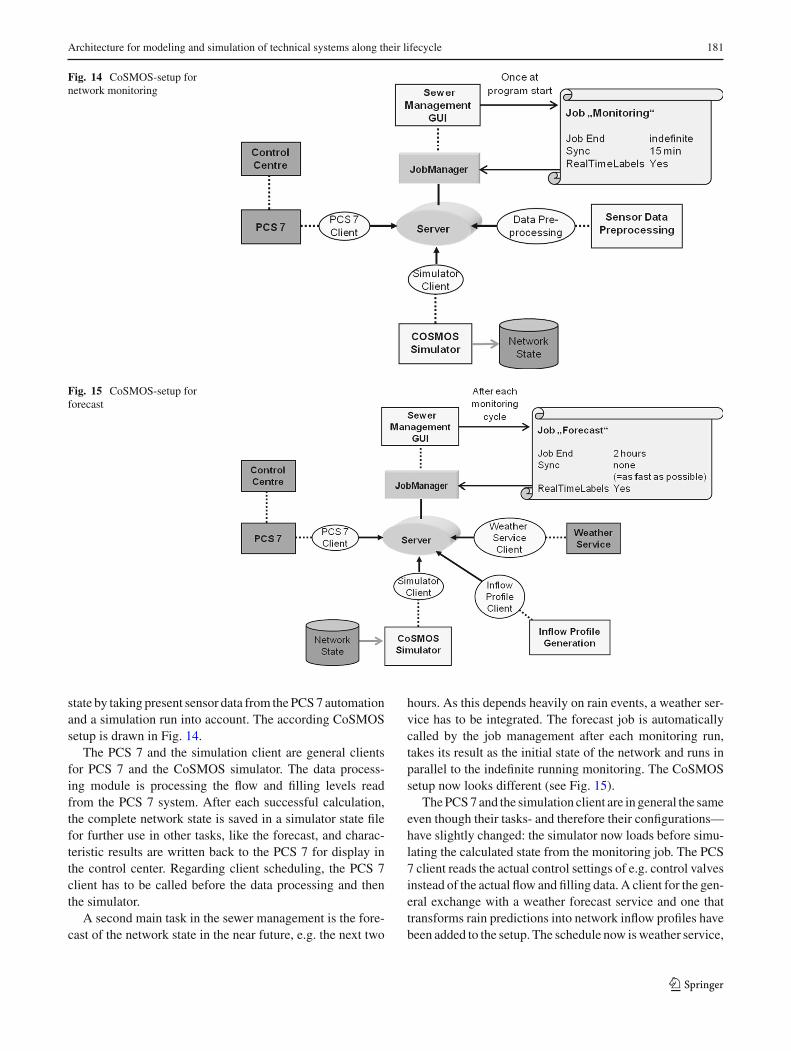
Fig. 14 CoSMOS-setup fornetwork monitoring

Fig. 15 CoSMOS-setup forforecast

state by taking present sensor data from thePCS7 automationand a simulation run into account. The according CoSMOSsetup is drawn in Fig. 14.

The PCS 7 and the simulation client are general clientsfor PCS 7 and the CoSMOS simulator. The data process-ing module is processing the flow and filling levels readfrom the PCS 7 system. After each successful calculation,the complete network state is saved in a simulator state filefor further use in other tasks, like the forecast, and charac-teristic results are written back to the PCS 7 for display inthe control center. Regarding client scheduling, the PCS 7client has to be called before the data processing and thenthe simulator.

A second main task in the sewer management is the fore-cast of the network state in the near future, e.g. the next two

hours. As this depends heavily on rain events, a weather ser-vice has to be integrated. The forecast job is automaticallycalled by the job management after each monitoring run,takes its result as the initial state of the network and runs inparallel to the indefinite running monitoring. The CoSMOSsetup now looks different (see Fig. 15).

ThePCS7and the simulation client are in general the sameeven though their tasks- and therefore their configurations—have slightly changed: the simulator now loads before simu-lating the calculated state from the monitoring job. The PCS7 client reads the actual control settings of e.g. control valvesinstead of the actual flow and filling data. A client for the gen-eral exchange with a weather forecast service and one thattransforms rain predictions into network inflow profiles havebeen added to the setup. The schedule now isweather service,

123

182 T. Schenk et al.

then inflow generation, then simulator and at last PCS 7 fordisplay.

Furthermore, when an operator wants to see the outcomeof changed control settings, he—nowmanually—triggers thesame forecast job as above after he changed the control set-tings in a separate operator panel.

6 Summary and outlook

The requirements on system simulations in the industrialcontext, from user and from developer perspective, cannotbe fully met by currently available commercial tools. Thechallenges of phase- and task-specific setups, partly withnon-expert users, amaximum inmodel and environment con-sistency and nonetheless an easy to maintain and extend soft-ware architecture demandmodular, very flexible architectureconcepts guaranteeing high-performance all the same.

In the presented structured approach, the challenges havebeen summarized in representative use cases. Subsequently,technical requirements on such an architecture concept havebeen deduced. The eventually presented CoSMOS concept isdesigned to face the challenges and use cases by implement-ing the technical requirements. All three industrial exampleshave been successfully realized in CoSMOS solutions basingon the same CoSMOS architecture.

Looking ahead, the co-simulation techniques and stan-dards, like FMI, will evolve further, resulting in the needfor more advanced sequence control algorithms and imple-mentation of new interfaces. To get the emerging variety ofco-simulation tasks under control is one of the upcominggoals of the next development steps.

Using distributed systems for a lot of common tasks is alsoone of the major trends in IT development. Thus, demandingdistributed simulation for the simulation user, especially forthe non-experts, is just obvious. The orchestration of distrib-uted simulation applications requires various techniques andalgorithms on all levels of the software. For example, web-based simulation demands for a simulation-specific browserfront end and a web service capable to process simulationtasks to the evaluation cores. On the other hand, distributingsimulation on solver level asks for exploitation of specificcall sequences and the structure of the equation system.

Another trend when performing industrial system sim-ulations is the extensive usage in concept and engineeringstudies. As the formulation and evaluation as mathemati-cal optimization problem is often not really understood, toocomplex or even impossible, multiple simulation runs areexecuted instead. The difference in the simulation runs rangefromdifferent boundary conditions to various sets of parame-ters and up to changes in the system topology. This procedureis not only very time consuming but also quite challenging inkeeping track of the outcomes and drawing the right conclu-

sions. A software environment that would support the userand deal automatically with some of those tasks would bemostly welcome.

This is just to name some of the main future challenges tocome,when facilitating future industrial systemdevelopmentand operation by use of simulations.

Open Access This article is distributed under the terms of theCreativeCommons Attribution 4.0 International License (http://creativecommons.org/licenses/by/4.0/), which permits unrestricted use, distribution,and reproduction in any medium, provided you give appropriate creditto the original author(s) and the source, provide a link to the CreativeCommons license, and indicate if changes were made.

References

1. Kim, J.-H., Lee, K., Tanaka, S., Park, S.-H. (eds.): Advancedmeth-ods, techniques, and applications in modeling and simulation. In:ProceedingsAsiaSimulationConference, Seoul,Korea,Nov. 2011,Springer (2012)

2. Hartmann, D., Mahler, M.: Integration of complex 3d-simulationswithin systems simulations using response surfaces. In: Proceed-ings of the NAFEMS Seminar Strömungsberechnungen (CFD) inder Systemsimulation (2013)

3. Loper, M.L.: Modeling and Simulation in the Systems EngineeringLife Cycle. Springer, Heidelberg (2014)

4. Matlab Simulink: http://www.mathworks.com/products/simulink/. Accessed 7 Nov 2014

5. AMESim: http://www.plm.automation.siemens.com/de_de/products/lms/imagine-lab/amesim/platform/. Accessed 7 Nov2014

6. Dymola: http://www.3ds.com/products-services/catia/capabilities*/systems-engineering/modelica-systems-simulation/dymola (last access 07. Nov 2014)

7. NASA roadmaps: TA11 TA11 Modeling, Simulation, and Infor-mation Technology and Processing, NASA Space TechnologyRoadmaps and Priorities 2012. www.nasa.gov/offices/oct/home/roadmaps/index.html. Accessed 7 Nov 2014

8. Follmer, M., Hehenberger, P., Punz, S., Rosen, R., Zeman, K.:Approach for the creation of mechatronic system models. In: Cul-ley, S.J., McAloone, B.J., Howard, T.J., Lindemann, U. (eds.)Proceedings of the 18th International Conference on EngineeringDesign ICED11, vol. 4, pp. 258–267. The Design Society, Kopen-hagen (2011)

9. Pohl, K., Hönninger, H., Achatz, R., Broy, M.: Model-Based Engi-neering of Embedded Systems: The SPES 2020 Methodology.Springer, Heidelberg (2012)

10. Brandstetter, V., Wehrstedt, J. C., Rosen, R., Pirsing, A.: Simu-lationsgestützte Entwicklung von Automatisierungssoftware. In:ATP-Edition, Fachmagazin für Automatisierungstechnische Praxis06/2013

11. Siemens AG, Power Plants, BENSONOnce-Through Heat Recov-ery Steam Generator. Order No. A96001–S90-A496-X-4A00,2006, Erlangen

12. Siemens Pictures of the future (2005) http://www.siemens.com/innovation/en/publikationen/publications_pof/pof_spring_2005/elements_of_life/simulated_water_networks.htm. Accessed 11Nov 2014

13. Pirsing, A., Rosen, R., Obst, B., Montrone, F.: Einsatz math-ematischer Optimierungsverfahren bei der Abflusssteuerung inKanalnetzen. In: GWF Wasser Abwasser, Jg.: 147, Nr. 5, Seite376–383 (2006)

123

Architecture for modeling and simulation of technical systems along their lifecycle 183

14. Modelica Association: The functional mock-up interface, https://www.fmi-standard.org/. Accessed 7 Nov 2014

15. Pumhössel, T., Hehenberger, P., Boschert, S.: On the advantages ofusing reduced system models in the model-based development ofmechatronic systems. In: Proceedings of 2ndWorkshop onMecha-tronic Design, Paris, France (2013)

16. SIMATIC PCS7 Operator System http://w3.siemens.com/mcms/process-control-systems/en/distributed-control-system-simatic-pcs-7/simatic-pcs-7-system-components/operator-system/pages/operator-system.aspx. Accessed 7 Nov 2014

17. TISC: http://www.tlk-thermo.com/de/softwareprodukte/tisc.html.Accessed 7 Nov 2014

18. ICOS: http://www.v2c2.at/icos/. Accessed 7 Nov 201419. Günther, M., Rentrop, P., Feldmann, U.: CHORAL - a one step

method as numerical low pass filter in electrical network analysis.In: Scientific computing in electrical engineering. In: Proceed-ings of the 3rd International Workshop, 20–23 August 2000,Warnemünde,Germany.Hrsg.:Rienen,U. van,Günther,M.,Hecht,D. Springer, Berlin, 199–215 (2001)

20. SIMATIC S7 PLCSim: http://w3.siemens.com/mcms/simatic-controller-software/de/step7/simatic-s7-plcsim/seiten/default.aspx. Accessed 7 Nov 2014

21. SIMATIC WINAC RTX: http://w3.siemens.com/mcms/programmable-logic-controller/de/software-plc/simatic-winac-rtx/seiten/default.aspx. Accessed 7 Nov 2014

22. SIMIT Emulation Platform: http://www.industry.siemens.com/services/global/de/it4industry/produkte/simulation/simit-emulation-platform/seiten/technische-daten.aspx. Accessed 7Nov 2014

23. Altpeter, R., Schiller, N., Weissenberger, B., Schweizer,R: Praktische Erfahrungen mit Online-Diagnosesystemen unterEinsatz des Kreislaufprogramms KRAWAL-modular, VDI Han-nover 03.06.03

123