Arbitraging Covered Interest Rate ParityDeviations and Bank Lending

LORENA KELLER a

August 2021

I propose and test a new channel through which covered interest rate parity (CIP) deviations can affect banklending in emerging economies. I argue that when there are CIP deviations, banks attempt to arbitrage them.This requires banks to borrow in a particular currency. When this currency is scarce, banks shift resourcesaway from lending to fund their arbitrage activities. Then, bank lending in the currency required to arbitragedecreases. I test this channel by exploiting differences in the abilities of Peruvian banks to arbitrage CIPdeviations and find evidence that supports the proposed channel.

aThe Wharton School, University of Pennsylvania. E-mail: lorenak@wharton.upenn.edu. I am indebted to thePeruvian Superintendencia de Banca y Seguros (Peruvian bank regulator - SBS) and the Superintendencia Nacionalde Administracion Tributaria (Office of income tax collection - SUNAT) for their collaboration in providing andcollecting the data. I am very grateful to Santiago Medina for excellent research assistance. This project has greatlybenefited from very helpful comments from Manuel Amador, Jules van Binsberger, Wenxin Du (discussant), MichaelRoberts, Nikolai Roussanov. It has also benefited from seminar participants at NYU Stern, Wharton, Wisconsin-Madison, NBER Summer Institute (International Asset Pricing), SED, Rome Junior Finance Conference, WFA. I amalso very thankful for the financial support from the Jacobs Levy Equity Management Center for Quantitative FinancialResearch, Wharton’s Dean Research Fund and Wharton’s Global Initiatives Research Program. All errors are my own.

1 Introduction

The covered interest rate parity (CIP) condition is the fundamental pricing equation for foreign ex-

change (FX) forward and swap contracts. However, as documented by Du, Tepper, and Verdelhan

(2018), there have been important deviations in developed economies that do not stem from outlier

events occurring during the financial crisis. Although for different reasons and with a different

dynamics, these deviations also exist in emerging economies. In this paper, I show that these

deviations can affect banks’ decisions on the currency composition of their lending in an emerging

market setting.

I start by proposing a channel through which CIP deviations can affect bank lending in a par-

tially dollarized economy. The channel is as follows. CIP deviations imply that there are arbitrage

opportunities. When these deviations exist, banks, who are the natural CIP deviations arbitrageurs,

attempt to arbitrage them.1 However, the arbitrage requires banks to borrow a particular currency.

When funding in that particular currency is scarce, banks need to either increase rates paid on

deposits or shrink funds in that currency that are being used in other activities, such as lending so

that these funds can be used to arbitrage. Then either because of an increase in rates in the currency

required to arbitrage or because of limited funds, lending in the currency required to arbitrage is

likely going to decrease relative to the one that is not required to arbitrage. Hence, arbitraging CIP

deviations can contribute to changes in currency mismatches in partially dollarized economies.

I test this channel by studying the relationship between arbitraging CIP deviations and bank

lending in Peru during a non-crisis period. I proceed in three complementary steps. First, I show

that banks’ FX and money market transactions suggest that they arbitrage CIP deviations. Second,

I show banks’ funding in the currency required to arbitrage CIP deviations becomes scarcer or

more expensive as CIP deviations increase. Finally, I exploit that banks have different arbitrage-

sensitivities to CIP deviations to show that banks that arbitrage more shift more the currency of

their lending in accordance to what is profitable to arbitrage.

The first step of the empirical analysis relies on how CIP arbitrage is executed. This is best

explained by reviewing first the CIP condition. Consider a local bank in Peru which has the

1Although banks cannot arbitrage them fully as else there would not exist CIP deviations.

2

opportunity to lend 1-month at the risk-free rate in dollars or in soles, the Peruvian currency.

Under CIP, the return of lending soles directly should equal the return of lending dollars and

simultaneously hedging the FX risk by selling dollars forward to convert them back to soles. The

return of the combination of lending dollars and hedging the FX is the soles synthetic rate. The

difference between the soles synthetic rate and the cash rate of lending directly is the cross-currency

basis. This basis measures the deviations from CIP.

Based on this description, the first step of the empirical analysis consists of measuring both at

the aggregate and at the bank level whether banks’ transactions are consistent with the expected

trades needed when banks arbitrage CIP deviations. In Peru, during my sample, CIP deviations

have oscillated between -2% and 2% (excluding the financial crisis). When the cross-currency basis

increases and the soles synthetic rate is greater than the soles cash rate, banks could theoretically

profit from borrowing soles in the money market and lending them synthetically. This entails

four transactions: (i) borrowing soles, (ii) selling soles and buying dollars spot, (iii) lending those

dollars, (iv) hedging the FX by selling dollars forward.

I use confidential data from Peru to show that as the cross-currency basis increases, banks

engage in more of each of these four transactions. These are only correlations but suggest that

banks’ transactions are consistent with arbitraging CIP.2 From the FX side, I have all of the forward

contracts of all banks in Peru. I also have all of their daily spot transactions. Using these two

datasets, I show that both in aggregate and at the bank level, banks buy more dollars spot and sell

more dollars forward as the cross-currency basis increases. From the money market side, I also see

banks’ interbank loans, financial obligations and investments. As expected, as the cross-currency

basis increases, banks borrow more soles and invest more dollars.

I complement the analysis with confidential information that has daily bank-level interest rates

paid on bank deposits. With this data, I find that as the cross-currency basis increases, banks

also increase the spread paid on soles term deposits, while they reduce this spread on dollar term

deposits. I also find that the bank’s soles liquid assets decrease and dollar liquid assets increase as

the cross-currency basis increases. This suggests that there is scarcity in the currency required to be

2As I describe later, an alternative explanation is that because banks hedge the FX exposure (Keller, 2020), and thehedging cost is measured by CIP deviations, banks decide their lending decisions based on the hedging cost measuredby CIP deviations.

3

funded to arbitrage CIP deviations. Yet, despite the scarcity of funds to arbitrage CIP deviations,

banks seem to allocate funds to arbitrage these deviations.

While I find that banks’ transactions are consistent with arbitraging CIP deviations, I also

find that banks differ significantly in terms of how much they respond to these deviations. I find

that after a 1pp increase in the USDPEN cross-currency basis, some banks respond by allocating

approximately 4% more of their assets to perform the arbitrage, while some others barely respond.

Because this heterogeneity is helpful when analyzing how arbitraging CIP deviations can affect

bank lending, I construct a bank-specific measure of banks’ ability to arbitrage CIP deviations.

This measure looks at how much each bank changes its forward position that is matched with

offsetting spot positions -two transactions required to arbitrage CIP deviations- after an increase in

the cross-currency basis.

I use this bank-specific measure on banks’ abilities to arbitrage CIP deviations to analyze the

possible impact of arbitraging CIP deviations on bank lending in soles and dollars. To reduce the

influence of shocks to the Peruvian economy that correlate with CIP deviations in Peru and bank

lending and to mitigate concerns that particular hedging choices of banks affect the cross-currency

basis, I instrument the USDPEN cross-currency basis with that of Mexico and Chile. Exploiting

the heterogeneity in banks’ abilities to arbitrage CIP deviations, I use a within firm-month analysis

to show that banks that allocate 1pp more of their assets to arbitraging CIP deviations increase

their dollar lending relative to soles lending by 11 to 40%3 after a 1pp increase in the USDPEN

cross-currency basis instrument. This increase in the difference between dollar and soles lending is

due to both, an increase in dollar lending and a decrease in soles lending. These results stem from

simultaneously comparing: (i) the lending of the same bank to the same firm at different levels

of CIP deviations and (ii) the lending of high arbitrage-intensive banks relative to less arbitrage-

intensive ones.

Comparing lending across banks with different arbitrage abilities is one of the ways I use to

try to alleviate the endogeneity problems that arise when trying to link arbitraging CIP deviations

to bank lending. Because CIP deviations are endogeneous, they correlate with macroeconomic

311% is the most conservative estimate I obtained, which holds when restricting the sample to firms borrowing insoles and dollars. When including the possibility of firms switching currencies, the estimates increase to 40%.

4

variables that can affect lending in different currencies by other means that might not relate to

arbitraging CIP deviations. Comparing how banks with different arbitrage abilities change their

lending to the same firm on the same month controls for changes in economic conditions that affect

all banks.

However, banks are heterogeneous and therefore shocks might not affect them in the same

degree. I take three steps to mitigate this problem. The first one is to use lagged bank controls to

control for bank heterogeneity in their balance sheets.4 The second one is to provide robustness

checks that narrow the analysis to the most similar banks. In this subset of banks, I analyze whether

those that arbitrage more lend more in dollars and less in soles as the basis increases. I find this

is still the case. Finally, the third step I take is to focus on whether the correlation between the

FX and CIP deviations affects the results.5 I refer to this channel as the FX channel. In Peru, the

value of the dollar is positively correlated with the cross-currency basis. As the sol depreciates, it

is expected that agents change their deposits from soles to dollars. This itself generates a shortage

of funding for banks in soles relative to dollars. Therefore, through independent channels, banks

could decide to lend less in soles and more in dollars as the cross-currency basis increases and the

sol depreciates.

Although it is very likely that the FX channel is at play, I show that this channel is likely

not the one behind the results on bank lending. If the FX channel described before explains the

results on bank lending, it must be that the depreciation of the sol affects more the banks that have

greater ability to arbitrage. That means that banks with greater ability to arbitrage also face greater

reduction of soles deposits when the currency depreciates and therefore end up lending more in

dollars relative to soles as the cross-currency basis increases and the sol depreciates. I do not find

evidence for this. The banks that arbitrage the most are not those experiencing greater reduction in

their soles and increase in dollar deposits after the currency depreciates. Moreover, controlling for

the possible differential effect in FX does not change the results.

Related to the FX channel, one could be concerned that changes in the FX change the demand

for loans of firms that have foreign trade. However, I do not find that changes in the demand for

4The results with and without bank controls are very similar.5This correlation is the only one I am aware that can affect the results. This correlation was established in Avdjiev,

Du, Koch, and Shin (2019).

5

loans of firms with foreign trade drive the results. I find that taking out these firms from the sample

yields similar results.

The results presented in this paper are robust to a series of alternative specifications, such

as using alternative measures of CIP deviations, using alternative samples and using alternative

exposure measures to sort banks by arbitrage intensity.

There are two main contributions of this paper to the literature on CIP deviations. First, to

the best of my knowledge, this is the first paper to propose and empirically test a channel through

which, by arbitraging CIP deviations, banks can change the currency composition of their lending

portfolios. Second, it complements the current literature by providing evidence that suggests that

CIP deviations might not only be an important phenomenon to asset pricing, but it can also affect

firms and households through changes in the currency composition of their loans.6

The literature on CIP deviations, has broadly addressed three topics. First, it has shown CIP

deviations have been common since the financial crisis. Examples of these papers include Baba,

Packer, and Nagano (2008); Baba and Packer (2009); Coffey, Hrung, and Sarkar (2009); Mancini-

Griffoli and Ranaldo (2011); Du, Tepper, and Verdelhan (2018), where Du, Tepper, and Verdelhan

(2018) highlights that this is not just a phenomenon seen during the financial crisis, but has been

present after the crisis. Second, the literature has also addressed why these deviations exist.

Examples are Du, Tepper, and Verdelhan (2018); Borio, Iqbal, McCauley, McGuire, and Sushko

(2018); Rime, Schrimpf, and Syrstad (2020); Wallen (2019)7. Finally, another set of papers study

the relationship between CIP deviations and other asset prices, such as the dollar (Avdjiev, Du,

Koch, and Shin, 2019) and credit spreads of corporate bonds (Liao, 2020).

6Papers that have studied CIP deviations outside asset pricing include Ivashina, Scharfstein, and Stein (2015) andAmador, Bianchi, Bocola, and Perri (2020). Ivashina, Scharfstein, and Stein (2015) show that, if CIP deviations areallowed in equilibrium, a shock to European global banks’ creditworthiness reduces their amount of loans in dollars,but not those in euros. Amador, Bianchi, Bocola, and Perri (2020) show that central bank’s FX policy can be costlierwhen it conflicts with the zero lower bound and CIP deviations are allowed. A difference with my paper is that in bothcases, the effects on the real economy are not directly due to arbitraging CIP deviations, but rather the result of shocksand policy in an environment where CIP deviations are allowed. Furthermore, the mechanism I propose is not relatedto shocks to the creditworthiness of banks or the zero lower bound.

7Du, Tepper, and Verdelhan (2018) establish a causal link to balance sheet constraints. Other papers have also addedother explanations for CIP deviations: bank credit risk and liquidity (Borio, Iqbal, McCauley, McGuire, and Sushko,2018), unaccounted real marginal funding costs (Rime, Schrimpf, and Syrstad, 2020) and imperfect competition(Wallen, 2019).

6

Most of the papers that address CIP deviations describe a setting that pertains to developed

economies. Because in most of the sample in this paper there were carry trade inflows in Peru,

the setting in this paper resembles that in Keller (2020) and Amador, Bianchi, Bocola, and Perri

(2020). In both cases, there are CIP deviations that arise in a setting with capital inflows and a

Central Bank that intervenes in the exchange rate to mitigate the FX appreciation.

A secondary contribution of this paper relates to the understanding of internal capital markets

in the banking system. This paper shows new empirical evidence on how internal capital markets

work for a bank that has to allocate scarce currency-specific liquidity between its lending and its

trading division. The empirical evidence has mostly focused on diversified firms (Lamont, 1997;

Shin and Stulz, 1998), bank holding companies (Houston, James, and Marcus, 1997; Houston and

James, 1998; Campello, 2002; Ashcraft and Campello, 2007; Cremers, Huang, and Sautner, 2011)

and global banks (Cetorelli and Goldberg, 2012a,b). Evidence of reallocation of funds within a

bank in a single country (Gilje, Loutskina, and Strahan, 2016; Ben-David, Palvia, and Spatt, 2017;

Slutzky, Villamizar-Villegas, and Williams, 2020) focuses on reallocation between branches in

different geographical locations. In this paper I study a different dimension of reallocation, and

this is between business divisions.

This paper is organized into five sections. Section 2 reviews the CIP condition. Section 3

describes CIP deviations in Peru and its banking system. Section 4 describes the data. Section 5 is

the main section of the paper. It presents the methodology and results. Finally, Section 6 concludes.

2 Review of CIP

This section reviews how CIP works and how arbitraging CIP deviations is done. It also introduces

definitions I use later on.

CIP is a non-arbitrage condition. It states that an investor should be indifferent between the

following two lending strategies: (i) lend a particular currency directly or (ii) lend it synthetically.

These are shown in Figure 1.

7

PEN: 1PEN (1+ yt,t+n)

n

PEN FtSt× (1+ yUSD

t,t+n)n

Invest at PEN Rate yt,t+1

1St

USD

1St

Buy

USD

/Se

llPE

N

1St× (1+ yUSD

t,t+1)nUSD

Invest at USD Rate yUSDt,t+1

Ft

Sell

USD

/B

uyPE

N

Figure 1: Example of Covered Interest Rate Parity (CIP)

This figure shows an example of CIP. In this example, an investor should be indifferent between two strategies. The first is to lend 1 sol (PEN)directly at the rate yt,t+1. When the investor does this, at t+1 the investor will have PEN 1+yt,t+1. This is the red strategy in the figure. The secondstrategy is highlighted in blue. This second strategy starts by using the PEN 1 that the investor has at time t and changing it for dollars (USD).Denoting the exchange rate as St PEN per USD, the investor will have USD 1

St. The investor lends these USD directly at the USD rate of yUSD

t,t+1.Hence, as of t + 1, the investor will receive 1

St× (1+ yt,t+1). CIP means that locking, as of time t, into a t + 1 exchange rate to convert the USD

return into PEN, should give the same PEN as if these PEN were lent directly. The t +1 exchange rate at which the investor can lock into in periodt is given by the forward exchange rate Ft . Using the Ft exchange rate (also quoted as soles per dollars) to convert the dollar loan proceeds to PEN,gives PEN Ft

St× (1+ yUSD

t,t+1). Therefore, under CIP, the return of the red and blue strategies are the same: 1+ yt,t+1 =FtSt× (1+ yUSD

t,t+1).

The first lending strategy of lending directly is shown in red in Figure 1. As an example,

consider the currency is soles (PEN). The n-year annualized rate of return of lending PEN directly

is yt,t+n and hence, at time t +n the investor will have PEN (1+ yt,t+n)n.

The second lending strategy, lending soles synthetically, is shown in blue in Figure 1. This

strategy begins with changing the PEN 1 that the investor has at time t to dollars (USD) at an FX

of St PEN per USD. The investor then lends the 1St

directly at the n-year annualized USD rate of

y$t,t+n. Consequently, in t + n, the investor will receive 1

St× (1+ yt,t+n)

n dollars. At time t, the

investor also uses forward contracts to lock into a t+n FX and convert the USD loan proceeds into

PEN. Denoting the forward FX as Ft,t+n, the investor converts its USD loan proceeds into PENFt,t+n

St× (1+ y$

t,t+n)n. Therefore, under CIP, the return of the red and blue strategies is the same:

(1+ yt,t+n)n =

Ft,t+n

St× (1+ y$

t,t+n)n︸ ︷︷ ︸

(1+y f wdt,t+n)

n

(1)

8

For simplicity, I denote the yearly return of this second strategy as y f wdt,t+n. This is the soles

synthetic rate (or forward-implied soles rate). From Equation (1) follows that:

y f wdt,t+n ≡

(Ft,t+n

St

)1/n

× (1+ y$t,t+n)−1 (2)

When there are deviations from CIP, Equation (1) does not hold and one lending strategy

provides a higher payoff than the other. The difference between the payoffs is known as cross-

currency basis, xt,t+n. In the literature, the cross-currency basis is typically defined in dollar terms:

xt,t+n = y$t,t+n−y$, f wd

t,t+n . Because the analysis in this paper is from the Peruvian banks’ perspective,

define the cross-currency basis in soles terms:

xt,t+n = y f wdt,t+n− yt,t+n (3)

As shown in Appendix A, the definition of the cross-currency basis in dollar terms (xt,t+n =

y$t,t+n− y$, f wd

t,t+n ) is equivalent to Equation (3).

When the cross-currency basis is positive (negative), the arbitrageur profits by lending (bor-

rowing) soles synthetically and borrowing (lending) them directly in the money market. The

specific transactions that the arbitrageur does consist of: (i) borrowing soles (dollars) directly, (ii)

converting these soles (dollars) to dollars (soles), (iii) lending in dollars (soles) while (iv) engaging

in a forward contract that sells the dollar (soles) loan proceeds to convert them to soles (dollars).

With the soles (dollars) received from the forward contract, the arbitrageur pays the soles (dollars)

it borrowed. What remains as profit, in terms of annualized return, is the cross-currency basis (in

absolute terms).

Intuitively, the sign of the cross-currency can be interpreted as relative scarcity of a currency.

The scarcity of a currency is the currency in which the market in general wants to borrow but not

lend. When the cross-currency basis is negative, there is relative abundance of soles compared

to dollars. Investors that might not have access to the soles cash rate are willing to lend soles in

the soles swap market at a lower rate than the soles cash rate. An analogous interpretation is that

the market generally wants to invest in soles but not borrow in soles. Instead, the market prefers

9

to borrow dollars but not lend in dollars. This last statement becomes clear when expressing the

basis in dollar terms (i.e. xt,t+n = y$t,t+n−y$, f wd

t,t+n ). In dollar terms, this is equivalent to a scarcity of

dollars. Investors that might not have access to the dollar cash rate are willing to borrow dollars in

the soles swap market at a higher rate than the cash rate.

3 Setting

This section describes the setting. Section 3.1 describes the behavior of CIP in Peru and in other

Latin American countries. Section 3.2 describes the Peruvian banking system.

3.1 CIP Deviations in Peru and Other Latin American Countries

Figure 2 plots the annualized cross-currency basis for 1-month contracts for the soles-dollar cur-

rency pair (USDPEN) and the average across other Latin American currency pairs between 2005

and 2013.8 The dotted gray line traces the “Chilean-Mexican basket,” which is the average basis

for Chilean (USDCLP) and Mexican peso (USDMXN) pairs. The orange line traces the “Latin

American basket,” which is the average basis for the Brazil real (USDBRL), Chilean peso (USD-

CLP), Colombian peso (USDCOP) and Mexican peso (USDMXN) against the dollar.

There are three takeaways from this figure. First, both for USDPEN and other emerging

markets, CIP deviations have been economically large. In Peru, it has oscillated between -2 and

2%, being many times above 1% in absolute value. Figure 2 shows that the average of the absolute

cross-currency basis for the USDPEN and for the Latin American basket has been approximately

0.60% during the sample of this paper. While this basis decreases when accounting for bid-ask

spreads, even accounting for these spreads, the average absolute value is 0.23%, which although

significantly smaller, it is still large. Moreover, at moments, even after transaction costs, the cross-

currency basis in Peru has also been above 1% in absolute value.

8I end the sample in February 2013 because after this date there were many regulations on the bank lending and onthe forward side that make it difficult to analyze later on the effects of arbitraging CIP deviations on bank lending.

10

-2

-1.5

-1

-.5

0

.5

1

1.5

2

Cro

ss-C

urre

ncy

Basi

s An

nual

Rat

e (%

)

2005m2 2006m2 2007m2 2008m2 2009m2 2010m2 2011m2 2012m2 2013m2

Peru (%)Chile, Mexico: Avg 1M, CCB (%)Brazil, Chile, Colombia, Mexico: Avg 1M, CCB (%)

Figure 2: CIP deviations in Peru and other Latin American countriesThis figure plots the USDPEN cross-currency basis against the average of the cross-currency basis of other Latin American currency pairs acrosstime. The orange line is the average of the cross-currency basis of Brazil, Chile, Colombia and Mexico. The dotted gray line is the average of thecross-currency basis of Chile and Mexico. The red line is the cross-currency basis of Peru. Although the level of Peru’s basis is closer to the averageof Brazil, Chile, Colombia and Mexico, its movements are more correlated to those in Chile and Mexico. All of these basis are computed usingthe local currency against the dollar and they are all 1-month basis. The shaded gray area represents the Global Financial Crisis. I am not showingthese months because I will not be using this sample to prevent an outlier period from affecting the results and because the significant deviationsaffect the scale.

Second, the USDPEN cross-currency basis is very correlated to the basis of other Latin Amer-

ican countries. The correlation between USDPEN and the Chilean-Mexican basket is 0.54 and

between USDPEN and the Latin American basket is 0.44.

Finally, excluding the financial crisis, most of the sample has negative cross-currency basis.

This is both the case in USDPEN and in the other Latin American countries. Hence, on average,

the profitable strategy for Peruvian banks has been borrow the local currency synthetically and

lend it directly. However, an important difference between the cross-currency basis in these devel-

oping economies and those in developed economies is that the cross-currency basis of developing

economies has switched signs at different times. This is very rare in developed economies, where,

with the exception of the New Zealand dollar and the Australian dollar, the cross-currency basis

of developed economies has been negative (see Du, Tepper, and Verdelhan (2018)). Possible

explanations for the different dynamics include dollarization and capital controls, which affect the

relative scarcity of dollars and soles to which different investors have access. Appendix B discusses

possible explanations for the different dynamics between developed and developing economies.

11

3.2 Peruvian banking system

The financial system in Peru is composed by banks and other types of financial institutions,

such as financial corporations, financial cooperatives known as “cajas” and leasing companies.

Because banks and other financial institutions have different regulations and because of greater

data limitation on financial institutions, I only focus on banks, which concentrate more than 90%

of the assets of the financial system. However, the results of this paper are robust to including the

whole financial system.

The commercial banking system in Peru is composed by 13 banks. The main business division

across Peruvian banks is household and commercial lending, which represents 62% of the banking

system’s assets. The other important division is trading, which makes investments in securities and

money market instruments.

Banks borrow and lend in soles and dollars. Borrowing and lending in local and foreign cur-

rency, a phenomenom known as “dollarization” is common across emerging economies.9 During

the sample period, loan and deposit dollarization averaged 59 and 55%, respectively. Firms and

households borrowing in dollars are, in its majority, not hedged. Indeed only a small fraction of

firms are exporters or have hedging instruments.

In contrast to firms and households, banks need to hedge their FX position. This is common in

emerging economies. They have limits on their total FX exposure, which is the sum of the spot and

forward position. 10 Banks can have long dollar spot positions as long as they are mostly offset

with forward positions.

Offsetting spot positions with forward positions is also what is required to arbitrage CIP devi-

ations. Then, one alternative interpretation of the results is that CIP deviations provide a profitable

way to hedge in a particular direction. Banks can exploit this and decide to hedge in the direction

which CIP deviations shows it is cheaper or more profitable for them to hedge.

9According to the Financial Soundness Indicators database (IMF), economies like Paraguay, Uruguay, Poland andTurkey had loan dollarization rates of 47%, 56%, 22% and 39%, respectively, as of 2018. In these countries, thesehigh rates of bank lending in foreign currency are explained by similarly high rates of foreign currency deposits fromlocal agents

10Limits on the total FX position is different than the limits on forward holdings studied in Keller (2020)

12

4 Data

The sample period for all datasets is February 2005 through February 2013. February 2005 is

when one of the main datasets, the credit registry, begins. February 2013 is the sample’s end date

because, from the end of 2013 until at least the start of 2016, there are many confounders. 11

First, I obtain market-based data on foreign exchange and money market data from Bloomberg.

I also use local interbank rates obtained from the Central Bank of Peru, Chile and Mexico. I have

used all of these to compute cross-currency basis across various currency pairs. The summary

statistics of the USDPEN cross-currency basis and other currency pairs is reported in Table A.I in

the Online Appendix.

I use the interbank rates to compute the cross-currency basis as the interbank rate is the key

and most liquid money-market instrument that Peruvian banks use for trading. The interbank dollar

rate in particular reflects better the cost of funding for Peruvian banks compared to Libor. This is

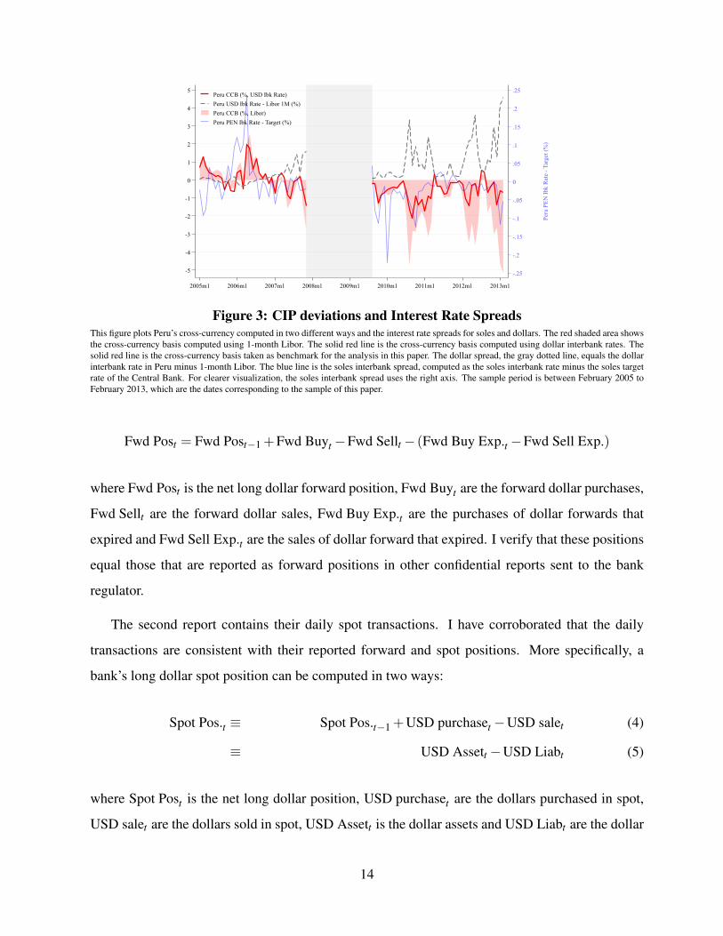
seen in Figure 3. At times when the the cross-currency basis was negative, the dollar interbank rate

has been greater than Libor. Therefore, as shown in Figure 3, using the dollar interbank rate yields

significantly smaller deviations from cross-currency basis than Libor.12

Second, I use bank-level data combined from a series of individual bank reports to the bank

regulator, SBS. These reports, mandatory for all banks operating in Peru, are largely confidential.

The first report entails the universe of their forward contracts. With these contracts, I can compute

the net long dollar forward position of a bank, which is the net long dollar position of all trades

that are currently active (i.e. not expired). More precisely, the net long dollar forward position of

a bank at time t is:11These confounders include a deep depreciation shock and various regulations that came with it. Given that the risk

aversion associated with the exchange rate also affects firms and households’ demand for borrowing dollars and thatthis is an unobservable variable that varies for each household and firm, it is also difficult to control for the changes incredit demand that could be associated with the exchange rate or expectations of the evolution of the exchange rate aswell as the risk premia.

12The higher dollar interbank rate compared to Libor is not due to risk aversion. On the contrary, during theseperiods of times, the credit default swap was at its minimum and there were capital inflows. An explanation for thehigher interbank dollar rate seems more linked to the FX intervention of the Central Bank. To mitigate the currencyappreciation from inflows, the Central Bank bought dollars in the spot market. These dollars were not sterilized, andtherefore, the Central Bank’s actions could have decreased the dollar liquidity. Such liquidity could not be easilysubstituted with dollar borrowing from abroad due to capital controls on inflows discussed in Keller (2020).

13

-.25

-.2

-.15

-.1

-.05

0

.05

.1

.15

.2

.25

Peru

PEN

Ibk

Rat

e - T

arge

t (%

)

-5

-4

-3

-2

-1

0

1

2

3

4

5

2005m1 2006m1 2007m1 2008m1 2009m1 2010m1 2011m1 2012m1 2013m1

Peru CCB (%, USD Ibk Rate)Peru USD Ibk Rate - Libor 1M (%)Peru CCB (%, Libor)Peru PEN Ibk Rate - Target (%)

Figure 3: CIP deviations and Interest Rate SpreadsThis figure plots Peru’s cross-currency computed in two different ways and the interest rate spreads for soles and dollars. The red shaded area showsthe cross-currency basis computed using 1-month Libor. The solid red line is the cross-currency basis computed using dollar interbank rates. Thesolid red line is the cross-currency basis taken as benchmark for the analysis in this paper. The dollar spread, the gray dotted line, equals the dollarinterbank rate in Peru minus 1-month Libor. The blue line is the soles interbank spread, computed as the soles interbank rate minus the soles targetrate of the Central Bank. For clearer visualization, the soles interbank spread uses the right axis. The sample period is between February 2005 toFebruary 2013, which are the dates corresponding to the sample of this paper.

Fwd Post = Fwd Post−1 +Fwd Buyt−Fwd Sellt− (Fwd Buy Exp.t−Fwd Sell Exp.)

where Fwd Post is the net long dollar forward position, Fwd Buyt are the forward dollar purchases,

Fwd Sellt are the forward dollar sales, Fwd Buy Exp.t are the purchases of dollar forwards that

expired and Fwd Sell Exp.t are the sales of dollar forward that expired. I verify that these positions

equal those that are reported as forward positions in other confidential reports sent to the bank

regulator.

The second report contains their daily spot transactions. I have corroborated that the daily

transactions are consistent with their reported forward and spot positions. More specifically, a

bank’s long dollar spot position can be computed in two ways:

Spot Pos.t ≡ Spot Pos.t−1 +USD purchaset−USD salet (4)

≡ USD Assett−USD Liabt (5)

where Spot Post is the net long dollar position, USD purchaset are the dollars purchased in spot,

USD salet are the dollars sold in spot, USD Assett is the dollar assets and USD Liabt are the dollar

14

liabilities. The subscript refers to time. I have daily data for each bank’s spot purchases and sales,

and I have monthly data for each bank’s assets and liabilities. I verify that at the end of the month,

each bank’s spot position computed by taking the previous month’s spot position and adding all

daily net dollar purchases (as in Equation (4)) equals the one computed by Equation (5).

The third report contains their daily positions on various money market accounts, including

interbank loans, financial obligations, investments in short term assets and liquidity ratios. The

fourth report includes the interest rates paid on various types of deposits as well as their balances.

Finally, I also use monthly public balance sheets.

Panel A of Table A.II in the Online Appendix shows the summary statistics of additional non-

balance sheet accounts, such as liquidity, profitability and FX derivatives. Notably, FX derivatives

are an important component of banks’ balance sheets, representing nearly 20% of their assets.

However, there is significant heterogeneity in the use of these derivatives. Some banks do not trade

FX forwards or swaps at all, while for others, the volume of these trades represents more than

80% of their assets.13 This table also presents summary statistics of “net matched position” and

β , which are discussed later, in Section 5.1. “Net matched position” is the spot position that has

been matched with the opposite transaction in the forward market. It takes a negative (positive)

value when the position is a net long (short) dollar spot that is matched with a net short (long)

dollars forward. The β is the estimated sensitivity of assets allocated to arbitraging CIP deviations

following a 1pp increase in the cross-currency basis.

Finally, I also use the credit register collected by the SBS. This constitutes the most granular

dataset on bank loans and, jointly with the spot and forward datasets, is the main dataset used in this

paper. The credit register, which is confidential, contains the monthly balances of all commercial

loans outstanding in dollars and soles to firms that during the sample period had a loan outstanding

of more than 300,000 soles (approximately 100,000 dollars) in aggregate with all the financial

system.

Almost 28,000 firms are included in the credit register. Table A.II Panel B shows the summary

statistics of these firms. Those labeled “small firms” have yearly sales below 20 million soles

13Interestingly, the three banks that arbitrage the most are not the banks that were most affected by capital controlsstudied in Keller (2020).

15

(approximately 6.5 million dollars). The medium firms have yearly sales between 20 and 200

million soles (6.5 to 65 million dollars) and the large firms have yearly sales above 200 million

soles14.

5 Methodology and Results

This section studies the effect of arbitraging CIP deviations on bank lending. I proceed in three

steps. First, in Section 5.1, I show that banks’ money market and FX transactions are consistent

with arbitraging CIP deviations but that some banks arbitrage more than others. Second, in

Section 5.2, I show that banks face balance sheet constraints when arbitraging these deviations,

suggesting that arbitraging CIP deviations could be using resources that otherwise would have

been used in lending. Finally, as a third step in Section 5.3, I provide evidence showing that

arbitraging CIP deviations is associated with changes in lending.

5.1 Step 1: Are banks’ transactions consistent with arbitraging CIP devia-

tions? Are there differences across banks?

To show that banks’ money market and FX transactions are consistent with arbitraging CIP de-

viations, I show that the correlations between CIP deviations and banks’ FX and money market

transactions are statistically significant and have the expected signs. I do this both at the aggregate

and at the bank-level. I allow the strength of these correlations to be asymmetric depending on

whether the cross-currency basis is positive or negative. I do this because, as per Section 2,

arbitraging a positive basis requires banks to borrow soles (PEN), whereas it requires dollar (USD)

borrowing when negative. Therefore, an arbitrageur is likely to increase soles borrowing when

the cross-currency basis is positive, as compared to when the basis is negative. More precisely, I

estimate Equations (6a) and (6b), which are aggregate and bank-level estimations respectively:

yt = θ0 +θ1CCBt ·1(CCBt > 0)+θ2CCBt ·1(CCBt ≤ 0)+ εt (6a)

14This corresponds to the “medium”, “large” and “corporate” category that the SBS uses to classify firms.

16

ybt = θ0 +θ1CCBt ·1(CCBt > 0)+θ2CCBt ·1(CCBt ≤ 0)+Bank FE+ εbt (6b)

In these equations, CCBt is the USDPEN cross-currency basis and 1(·) is the indicator function.

The dependent variables, yt and ybt are money-market or FX positions, scaled by total assets.

Money-market positions include interbank borrowing, obligations with financial institutions15,

investing in the Central Bank’s certificate of deposits or sovereign debt, investing in other bonds.

FX positions include FX spot and forward. yt aggregates the data at the month-level while ybt is at

the bank-month level. Bank fixed effects (“Bank FE”) are also present in the bank-level regression.

The coefficients of interest are θ1 and θ2. They capture the correlations between yt and the basis

when it is positive and when it is negative, respectively.

Table 1, Panel A shows the expected results. These are split into three groups: borrowing, FX

and lending. As the cross-currency basis increases, arbitraging banks: (i) increase their borrowing

in soles and decrease their borrowing in dollars; (ii) buy more dollars spot and sell dollars forward;

(iii) lend more in dollars and less in soles. Asymmetry is also present and in the expected direction,

both in terms of magnitude and statistical significance. When the basis is positive, banks borrow

more in soles than when it is negative. Banks also buy more dollars spot, sell more dollars forward

and invest more in dollars when the basis is positive than when it is negative.

The magnitude of the spot and forward coefficients (Table 1, Columns 5 and 6) are worth

highlighting. In absolute terms, they are two to three times as large as those in the borrowing

and lending sides. For example, when the basis is positive, a 1 pp increase in the cross-currency

basis is associated with a 3.34 pp increase in the spot dollar long position, but financial obligations

in soles only increase by 1.13 pp and interbank loans by 0.31. This means that banks are only

funding approximately 40% of their dollar purchases with new soles borrowed with interbank

loans and financial obligations; the analogous occurs with dollar borrowing when the basis de-

creases. Accordingly, banks will need to fund their dollar purchases as the basis increases through

other sources, which can include bank deposits or directly reducing funding in different business

divisions (i.e., commercial and personal lending).

15This includes from other financial institutions that are not banks, the Central Bank and financial institutions abroad

17

At this point, a question that arises is who is on the other side of the arbitrage? Although I

do not have information on the counterparty for all transactions involved, I do have counterparty

information for forward contracts. I find that foreign investors are on the other side of arbitrage

transactions. This is not the case for local investors.16 An explanation for this is market seg-

mentation between foreign and local banks. Because of capital controls and because soles are not

deliverable abroad, foreign investors will find more costly and difficult to arbitrage CIP deviations

(see Appendix B for details on market segmentation). What they can do instead is engage in carry

trade using forward contracts, which is something local banks cannot do because regulation limits

their FX exposure.

Shifting to the bank-level results, Panel B of Table 1 shows that the transactions are still

consistent with arbitraging CIP deviations but results are less robust than the aggregate estimations.

This is expected if there is heterogeneity in banks’ arbitraging activities and not all banks arbitrage

CIP deviations.

To further analyze differences in banks’ ability to arbitrage CIP deviations, I compute bank-

level sensitivities of the share of the banks’ assets likely used to fund arbitrage after a change in the

cross-currency basis. To do so, I first construct a bank-level measure that proxies for the share of a

bank’s assets invested in arbitraging the basis. Then, I use this measure to compute bank-specific

sensitives.

Construction of arbitrage proxy. To construct the proxy for the share of a bank’s assets invested

in arbitraging the basis, I compute a daily measure of the forward and swap position of a bank that

is offset by its spot position.17 The amount of a bank’s long forward position that is effectively

matched with its short spot positions is the proxy. I call this variable the “matched position” of

16This is shown in Table A.III in the Online Appendix. This table shows the estimated correlation between thecross-currency basis and the share of dollars forward local banks buy, splitting the sample between foreign and localinvestors. When trading with foreign investors, a 1pp increase in the cross-currency basis is associated with a 4ppdecrease in local banks’ share of dollar purchases from foreign investors. This result is not present in trades withlocal investors. Because local banks need to sell dollars forward to arbitrage an increase in the cross-currency basis,the decrease in the share of dollar purchases from foreign investors is consistent with local banks arbitraging thecross-currency basis from foreign investors.

17I compute positions, that is stock, rather than flows, for two reasons. First, I want to associate changes in thecross-currency basis with changes in these positions. This is given by the coefficient in the regression between thesepositions and the cross-currency basis. Second, because when a forward contract expires, a bank needs to renew itto keep its spot position hedged with the forward position, the purchases and sales of forward contracts could not berepresentative of whether a bank is arbitraging as these could be due to renewals of expiration of forward contracts.

18

a bank. This measure can capture arbitrage position because any CIP arbitrage position requires

banks to offset their forward positions with spot positions. Although banks borrow and lend as

part of arbitraging CIP deviations, I rely only on the FX positions because they are a cleaner proxy

than the bank’s use of the money market.18 Formally, I define the matched position of a bank as

follows:

Matchedbt =

+min{|Spot Pos.|, |Fwd+Swap Pos.|} , if Fwd+Swap Pos. > 0∧Spot Pos. < 0

−min{|Spot Pos.|, |Fwd+Swap Pos.|} , if Fwd+Swap Pos. < 0∧Spot Pos. > 0

0 , if sgn(Fwd+Swap Pos.) = sgn(Spot Pos.)

(7)

Because the matched position of a bank (Matchedbt in Equation (7)) is the amount of a bank’s

long dollar forward position that is offset with short spot positions, it is computed as the minimum

between the absolute value of the spot position and the forward position. Matchedbt is positive

when a bank has a net long dollar forward position that is offset and a net short dollar spot position

(the first case in Equation (7)), and negative when the converse occurs (the second case) 19. When

banks do not offset spot positions with forward positions, they are not arbitraging so Matchedbt is

zero. Because arbitraging CIP deviations involve selling dollars spot and buying dollars forward

when the cross-currency basis is positive, the expected correlation between Matchedbt and CIP

deviations is negative.

In any case, because banks need to hedge their forward with their spot position, when a bank decides not to renew aforward position, it will also need to change its spot position.

18Identifying a set of money market accounts as a measure of arbitrage activity that is valid across banks and throughtime is challenging. For example, divesting liquid soles assets can be equivalent to borrowing soles at a very low rate.This can vary endogenously through time and across banks. Furthermore, the investment leg could be performed withother less-traditional assets like lending to the local corporate or household sector. To sum up, there is a higher degreeof uncertainty on which accounts are used for the borrowing and investing legs of arbitrage. On the other hand, theuse of the FX market is unavoidable when arbitraging CIP deviations, as the bank has to swap currencies and hedgethe operation. Such actions will always be reflected in the matched position of a bank. It is not coincidence, that boththe spot and forward + swap positions of banks had the strongest and most robust correlation with the cross-currencybasis in Table 1.

19In this case, the bank has a net short dollar forward position (Fwd+Swap Pos.<0) and a net long dollar spotposition (Spot Pos.>0). Analogously, it is matching its short forward and long spot positions by an amount equal tothe size of the smallest one. This is the exact type of strategy that a bank performs when it arbitrages CIP and the basisis positive, as arbitrage requires buying dollar spot and selling dollar forward.

19

Computation of bank-specific sensitivities. I use Matchedbt to estimate β , the measure I use to

compare banks’ abilities to arbitrage. I estimate β separately for each bank by using the following

time-series regression:

(MatchedAssets

)bt= αb +βbCCBt + εbt ∀b ∈ B (8)

where t indexes months, b indexes a particular bank and B is the set of all banks in the sample.

Month-level variables were calculated as the averages of their daily counterparts.

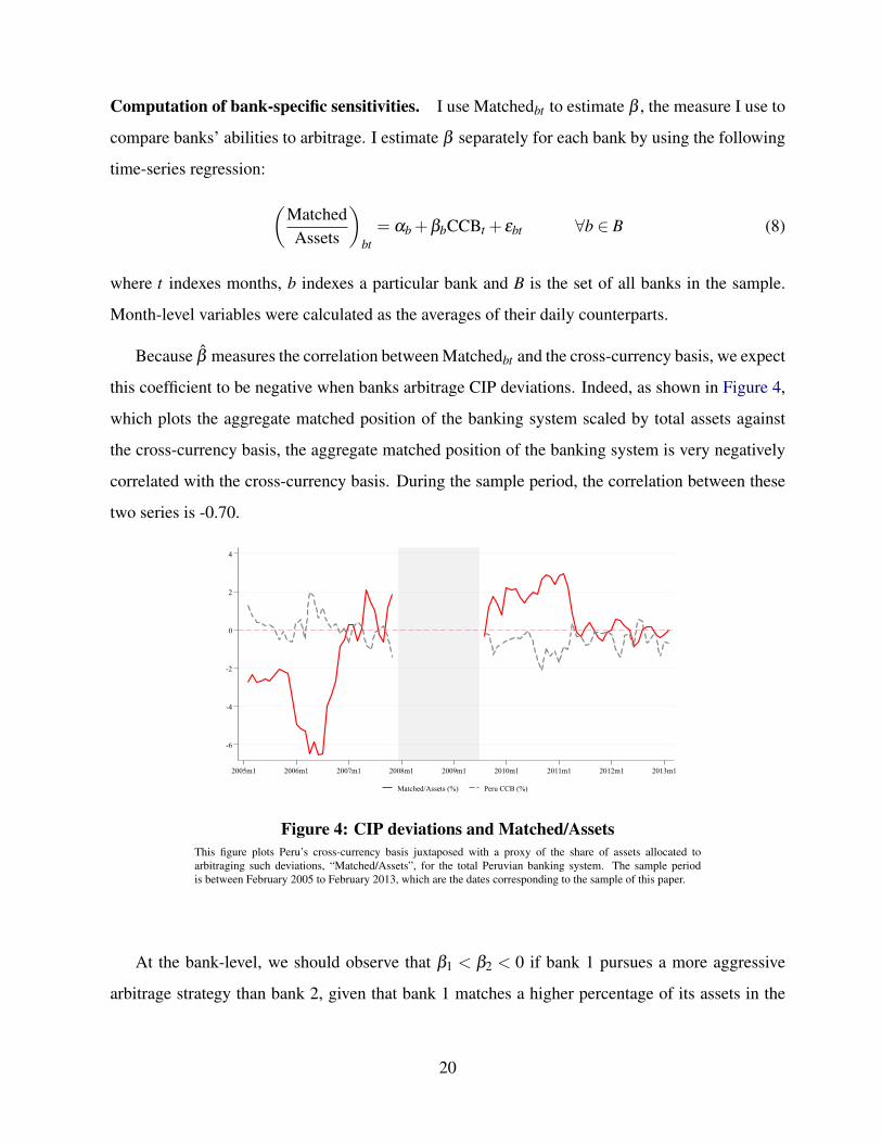
Because β measures the correlation between Matchedbt and the cross-currency basis, we expect

this coefficient to be negative when banks arbitrage CIP deviations. Indeed, as shown in Figure 4,

which plots the aggregate matched position of the banking system scaled by total assets against

the cross-currency basis, the aggregate matched position of the banking system is very negatively

correlated with the cross-currency basis. During the sample period, the correlation between these

two series is -0.70.

-6

-4

-2

0

2

4

2005m1 2006m1 2007m1 2008m1 2009m1 2010m1 2011m1 2012m1 2013m1

Matched/Assets (%) Peru CCB (%)

Figure 4: CIP deviations and Matched/AssetsThis figure plots Peru’s cross-currency basis juxtaposed with a proxy of the share of assets allocated toarbitraging such deviations, “Matched/Assets”, for the total Peruvian banking system. The sample periodis between February 2005 to February 2013, which are the dates corresponding to the sample of this paper.

At the bank-level, we should observe that β1 < β2 < 0 if bank 1 pursues a more aggressive

arbitrage strategy than bank 2, given that bank 1 matches a higher percentage of its assets in the

20

direction predicted by arbitrage when the basis changes by 1 pp. Consequently, I interpret the

estimated βb coefficient as proxy of bank b’s intensity of arbitrage abilities/activities.

Estimating Equation (8) separately for each bank yields considerable heterogeneity in the

resulting coefficients. Although I cannot show the regression results for each bank due to confiden-

tiality agreements, Figure 5 shows the smoothed distribution of the coefficients. A concentration

of banks is shown near-zero β s (low-arbitrage banks), whereas another group of banks has β s that

are much larger than or significantly different from zero (high-arbitrage banks). The estimated

coefficients of the low- and high-arbitrage banks lie in approximate ranges of [-0.2,0] and [-4.8,-

1.6], respectively.

.05

.1

.15

.2

.25

Den

sity

-6 -4 -2 0 2Estimated beta coefficient

kernel = epanechnikov, bandwidth = 0.9601

Figure 5: Smoothed density of the estimated β coefficientsThis figure shows the smoothed distribution of the coefficients. It does not show the individual regressionresults for each bank due to confidentiality agreements.

I verify that β s effectively capture arbitrage ability. The FX and money-market transactions

of banks that arbitrage more (have higher absolute value β ) are more consistent with arbitraging

CIP deviations than those that arbitrage less. This is shown in Table 1 Panel C and Panel D. These

panels show the results of splitting banks into high and low-arbitrage banks and estimating the

same regressions than those in Panel B for each group. As expected, the estimated coefficients

for the arbitrage accounts are larger in the group of high-arbitrage banks, than they are in the

low-arbitrage group. More specifically, the coefficients for high-arbitrage banks (Panel C) are,

generally, very consistent with banks that are using these accounts for arbitrage, both in terms of

21

sign, significance and asymmetry. However, the coefficients for the low-arbitrage banks (Panel

D), are either: (i) opposite to arbitrage; (ii) non-significant; or (iii) smaller than their counterparts

from Panel C. These findings provide evidence suggesting that β s are a good measure to proxy for

banks’ arbitrage activity.

5.2 Step 2: Is the currency needed to arbitrage CIP deviations scarce?

Section 5.1 shows banks’ transactions are consistent with arbitraging CIP deviations. This section

examines whether the currency that banks need to borrow to arbitrage is scarce at the time that

CIP deviations exist. If this is the case, it means that banks are allocating a scarce resource to

arbitraging CIP deviations and it can therefore affect funding of that currency in other business

divisions, such as their commercial lending division. For example, consider that the cross-currency

basis is positive. Arbitraging these deviations requires borrowing soles. Banks can source funds

internally or externally. On one hand, if banks choose to source funds internally, they will be

reallocating soles resources away from other divisions. If this division is the lending division,

soles lending falls. On the other hand, if banks source externally, they need to pay more for soles

funding. The result is likely higher soles lending rates that can induce firms to substitute their soles

borrowing for dollar borrowing. The converse happens when the cross-currency basis is negative.

A first indication that the currency required to arbitrage can be scarce involves analyzing

what happens to the soles and dollar interbank spreads (with respect to the target rate) when the

cross-currency basis is positive in contrast to when it is negative. As shown in Figure 3, the

soles interbank rate increases above the Central Bank’s target rate when the cross-currency basis

is positive and arbitraging CIP deviations require banks to borrow soles. Similarly, the dollar

interbank rate increases above Libor when the cross-currency basis is negative and arbitraging CIP

deviations require banks to borrow dollars. The positive correlation between the cross-currency

basis and the soles spread, as well as the negative correlation between the basis and the dollar

spread occurs despite the CIP deviations are already computed with interbank soles and dollar

rates. Therefore, although these changes in interbank rates close the cross-currency basis gap, the

CIP deviations are much larger than the changes in rates.

22

More formally, I present evidence that banks seem to face borrowing constraints in the currency

required to arbitrage by replicating the regressions of the previous section (Equations (6a) and (6b))

using interest rate spreads20 and liquidity ratios. Table 2 presents the results. In aggregate, a 1pp

increase in the cross-currency basis is associated with an increase of 0.3pp in the soles term deposit

spread and a decrease in 2.5pp decrease in the share of soles liquid assets21. Analogously, a 1pp

decrease in the cross-currency basis is associated with an increase between 0.35 and 0.57pp in the

dollar spread and an increase of 1.61 to 3.75pp in the share of dollar liquid assets22.

Although a possible explanation for the scarcity of the currency required to arbitrage could

be the demand of funds to arbitrage CIP deviations, it is possible that CIP deviations are not the

main driver of these correlations. CIP deviations correlate with other macroeconomic factors (eg.,

the FX and interventions by the Central Bank in the FX market) and therefore, I do not claim

causality. On one hand, estimating bank-level regressions of Table 2 for for high and low-arbitrage

banks (Panels C and D) shows that the estimated coefficients for the interest rate spreads do not

differ much between the two groups.23 On the other hand, the liquidity ratios’ coefficients are

notably larger and more significant for the high-arbitrage banks, whereas the low-arbitrage banks

have non-significant coefficients that are also smaller in absolute value. This finding suggests that

banks’ arbitrage is driving part of these liquidity changes.

However, importantly, the origin of the scarcity of liquidity is not relevant for this paper.

What matters is that the currency required to arbitrage CIP deviations is scarce when banks want

to arbitrage. This means that banks are optimizing under funding constraints and therefore, to

20I use are interest rate spreads over the monetary policy target rate so as not to pick up changes in monetary policy.For soles rates, I use spread with respect to the Peruvian Central Bank’s target rate. For dollar rates, I use the spreadwith respect to the Fed’s target rate. Using the spread with respect to Libor yields very similar results. I compute thisspread for two sources of financing that are likely used for arbitrage: new term deposits and interbank loans. AlthoughI use interbank rates to compute CIP deviations as private conversations with trading desks in Peru suggested theseare the rates I should use to compute CIP deviations as these are both borrowing and lending rates for banks, I havealso done robustness checks using with different rates, such as Libor, risk-free rates computed by van Binsberger,Diamond, and Grotteria (2021). The results are robust to these changes in computation of the cross-currency basis.

21This ratio is a standard metric, used widely to assess whether banks can have liquidity to pay for new or pastcommitments. A decrease in this ratio means that banks will have less liquidity that can be used for new lending.

22Notice that a direct channel that affects the share of liquid assets is arbitraging CIP deviations. Arbitraging CIPdeviations must involve buying a particular currency in spot and this mechanically affects liquid assets. For example,when the basis increases, the arbitrage involves buying dollars spot. Thus, banks are giving up cash in soles andreceiving cash in dollars.

23Regressions for the interbank loan spreads are not estimated again at the bank-month level because I do not havethe interest rates paid for these loans at the bank level.

23

arbitrage CIP deviations, they need to reallocate funds internally or pay more to obtain funds

externally. Either possibility can impact bank lending and this is what is going to be tested in the

next section, Section 5.3.

5.3 Step 3: How does arbitraging CIP deviations affect bank lending in soles

and dollars?

This section examines whether the arbitrage of CIP deviations in a context where there seems to

be scarcity in the funding currency can affect bank lending in soles and in dollars. Section 5.3.1

presents the methodology and Section 5.3.2 presents the results.

5.3.1 Methodology

Estimating the effect of arbitraging CIP deviations on bank lending is challenging. First, CIP

deviations are affected by macroeconomic shocks. Shocks to the economy affect CIP deviations

and banks’ decisions to lend in different currencies. These shocks also affect firms’ investment op-

portunities and therefore their credit demand. Therefore, controlling for the effect of these shocks,

both from the bank side as well as from the firm side is crucial. Second, banks’ lending decisions

themselves could affect CIP deviations. Given that they operate in the FX and commercial lending

markets, their actions affect both markets. A bank that decides to lend in a particular currency and

simultaneously hedge the FX risk could change its demand in the forward market and ultimately

affect USDPEN cross-currency basis.

The main regression specification, shown in Equations (9a) and (9b), addresses these problems

in three ways. First, it compares how banks with different abilities to arbitrage CIP deviations

change their lending in dollars and soles following changes in the cross-currency basis. Then,

as long as shocks affect all banks equally, banks’ loan supply should not be affected by such

shocks. Second, it focuses only on firms with multiple bank relationships (more than 70% of my

sample) and compares how banks with different abilities to arbitrage CIP deviations change their

lending to the same firm on the same month. Performing a within firm-month analysis (i.e. using

24

firm-month fixed effects) and only comparing changes of bank lending to the same firm reduces

concerns that the results could be driven by changes in firms’ credit demand. Third, it instruments

the CIP deviations in Peru with those in Mexico and Chile. Using as instrumental variable (IV) the

cross-currency basis of Mexico and Chile not only reduces the influence of shocks to the Peruvian

economy on the estimation results, but also prevents the results from being biased from Peruvian

banks’ trading decisions in the FX market that affect the USDPEN cross-currency basis. More

precisely, I estimate the following two-stage least squares model:

CCBPerut−1 ×Arb.Intensityb = γ0 + γ1CCBChMex

t−1 Arb.Intensityb +X ′b,t−1Θ+ψb +υb,t−1 (9a)

yb f t =α0 +α1 CCBPerut−1 ×Arb.Intensityb

∧

+ψb f +ψ f t +X ′b,t−1Ψ+ εb f t (9b)

where y is the observed credit outcome (log of USD, PEN, total, share of USD loans) given

by bank b to firm f on month t24; CCBPerut−1 is the one-month lagged cross-currency basis of US-

DPEN; CCBChMext−1 is the average one-month lagged cross-currency basis of Chilean and Mexican

peso against the dollar (USDCLP and USDMEX, respectively); -β is the negative of the bank β

estimated in Section 5.1 and measures the bank arbitrage intensity level25; Xb,t−1 is a vector of one-

month lagged bank controls; ψb, ψb f and ψ f t refer to bank fixed effects, bank-firm fixed effects

and firm-month fixed effects, respectively. Equations (9a) and (9b) refer to the first and second

stage of the two-stage least squares model, respectively.

I use the average between the one-month USDCLP and USDMEX cross-currency basis for

two reasons. The first reason is that a condition for the instrument to be valid is that it must be

highly correlated with the USDPEN cross-currency basis. The USDCLP and USDMEX basis are

24For this regression, I sum across all types of loans for each bank-firm-month. Each observation present includesonly firms that have positive total credit with a bank. However, a firm could be borrowing only soles or only dollarsat one point in time. To keep the same number of observations between soles and dollar loans and prevent fromconsidering different samples of firms when looking at soles versus dollar loans, before taking logs I add 1 sol(approximately 0.33 dollars) to all loan balances. Moreover, to make loan balances compatible across time, the dollarloan balances use a constant FX as of the start of the sample, February 2005. I have also performed robustness checkswhere I do not add 1 sol to the loans. The conclusion remains, although the coefficients are smaller. Similarly, I havealso done robustness checks without adjusting the FX to have a constant FX. The results remain.

25I use the negative value as to have β in positive numbers and facilitate interpretation. Recall that, as arbitragepredicts, these β s are negative. Then a greater value of −β is indicative of a bank that arbitrages.

25

the two Latin American currencies whose correlation with the USDPEN cross-currency basis is the

strongest. As shown in Table A.I, the average basis of USDCLP and USDMXN has a correlation

of 0.54 with the USDPEN cross-currency basis. This is aligned with the first-stage results that I

present later that suggest that there is not a weak instrument problem. The second reason is that

Peruvian banks barely trade these currencies and are thus unlikely to affect their prices. Fewer than

1.1% of all of the forward contracts that banks in Peru traded were USDMXN or USDCLP.26

The role of the bank-firm fixed effects is to control for time-invariant characteristics between a

bank and a firm. They also control for time-invariant differences across banks. This is important

because shocks that correlate with CIP deviations may not affect all banks in the same way. If

these shocks are also correlated with banks’ abilities to arbitrage, the results on bank lending may

be driven by the shock that correlates with CIP deviations rather than arbitraging CIP deviations

by banks. Controlling for time-invariant characteristics of banks as well as their relationships

with firms helps mitigate this concern. Because the fixed effects do not capture the time-varying

component of banks’ characteristics, I also add lagged time-varying bank controls. These controls

include soles and dollar deposits scaled by total assets, log of total assets, return over assets and

share of liquid assets in soles and dollars. However, I find that the regressions without lagged bank

controls yield very similar results.

The result of this specification is that the coefficient of interest, α1, measures the percentage

increase in bank lending of increasing arbitrage intensity by 1 (i.e increasing -β by 1) after a one

percentage point increase in the cross-currency basis when lending to the same firm on the same

month. Then α1 simultaneously compares (i) the lending of the same bank to the same firm at

different levels of CIP deviations and (ii) the lending of high arbitrage-intensive banks relative to

less arbitrage-intensive ones.

Although the baseline regression specification addresses various concerns, one could still be

worried about the heterogeneity across banks and the correlation between the cross-currency basis

and other macroeconomic shocks. To alleviate these concerns, later I also redo the analysis

26I compute these numbers from the dataset that includes all forward transactions of banks. Included here are alsotrades between MXN and CLP against PEN.

26

narrowing the sample to the most similar banks as well as analyze how changes in the FX, a

variable known for comoving with CIP deviations, affects the results.

I perform various other robustness checks after presenting the baseline results. These checks

include using alternative specifications, different samples, different computations of the cross-

currency basis, and checks on the standard errors.

5.3.2 Results and Robustness

Below I discuss the baseline regression results as well as results from performing additional

robustness checks.

Baseline results. The main takeaway from estimating the baseline regression is that an increase

in the cross-currency basis increases lending in dollars and reduces it in soles. These results are all

significant at 1%. They are also consistent across alternative specifications and economically large.

Banks that allocate 1pp more of their assets to arbitraging a 1pp increase in the cross-currency basis

increase their dollar lending by 11 to 40% relative to their soles lending. Decomposing this result

into soles and dollar borrowing, I find that this result is not only driven by an increase in dollar

lending, but also a decrease in soles lending. The range provided depends on the sample. The most

conservative result of 11% is when including only firms that were already borrowing in dollars and

soles. The largest result derives from including all firms, and this is what I take as benchmark. In

net terms, this represents a change in the currency denomination of the loans and a small change

in total loans.

Table 3 shows the first-stage results for various specifications, including the baseline specifica-

tion (Column 3). These results show that the instrument is statistically significant and stable across

specifications. Its strong correlation with USDPEN cross-currency basis also indicates the absence

of a weak instrument problem.

Table 4 shows the second-stage results for the baseline specification using four different de-

pendent variables: log of dollar loans, log of soles loans, log of total loans, the share of dollar

loans and the difference between log of dollar and log of soles loans. The first five columns in both

tables correspond to the OLS results, while the last five correspond to the IV results. The first-stage

27

results for this specification are those in Column 3 of Table 3. These are the results including all

firms. The most conservative results, that result from only considering those borrowing in soles

and dollars are found in row 5 of Table A.VI in the Online Appendix.

Both types of model, OLS and IV, show the same pattern and statistical significance, but the

differences between OLS and IV show a consistent negative bias. The bias is as expected and

can be explained as follows. A bank that decides to lend more dollars, by regulation, will need

to hedge.27 Unless the bank borrows and lends in the same currency, the bank will need to hedge

by selling dollars forward. As market maker, when the bank sells dollars forward, it will set

downward pressure to the forward outright (Ft,t+n in Equation (1)) and decrease the cross-currency

basis. This ultimately leads to lower cross-currency basis, higher dollar lending and lower soles

lending (if lending more in dollars means banks prefer to lend less in soles); and hence, goes

against finding a result through the mechanism proposed in this paper. Then, as expected, OLS

estimates are significantly lower than the IV estimates.

I perform various robustness checks. In sum, the results are widely robust to various alternative

specifications and samples, as well as they are robust to controlling for changes in the FX (a shock

that correlates with CIP deviations). Below I describe these checks in more length. The tables for

all robustness checks are in the Online Appendix.

Robustness check regarding the FX. Avdjiev, Du, Koch, and Shin (2019) document that the

value of the dollar is correlated with the cross-currency basis. Peru is no exception. Figure 6

shows that the value of the dollar (i.e. the FX) is correlated with CIP deviations in Peru.28 The

positive correlation between the FX and the cross-currency basis that is seen for the USDPEN

means that when soles (PEN) depreciate, the cross-currency basis increases.

This correlation between the FX and the cross-currency basis can confound the effects of

arbitraging CIP deviations because, through independent channels, a depreciation of the local

currency and an increase in the cross-currency basis can both generate an excess supply of dollar

27By regulation, banks need to match the currency of their assets with those of their liabilities.28Avdjiev, Du, Koch, and Shin (2019) show that in developed economies, the value of the dollar is negatively

correlated with the cross-currency basis. However, in emerging economies this correlation is positive. It is out of thescope of this paper to indicate why this is the case. Instead, I take this correlation as given.

28

-3

-2

-1

0

1

2

12-m

onth

s C

hang

e in

USD

PEN

CC

B (p

p)

-15

-10

-5

0

5

12-m

onth

s %

Cha

nge

in U

SDPE

N

2005m2 2006m2 2007m2 2008m2 2009m2 2010m2 2011m2 2012m2 2013m2

∆12m USDPEN Spot (%)∆12m USDPEN CCB (pp)

Figure 6: CIP deviations and FXThis plot shows the yearly changes in USDPEN cross-currency basis against the yearly changes in FX. Thered line corresponds to the changes in the spot while the gray line corresponds to changes in the cross-currencybasis. The cross-currency basis corresponds to the 1-month basis. The shaded gray area represents the GlobalFinancial Crisis. I am not showing these months because I will not be using this sample to prevent an outlierperiod from affecting the results and because the significant deviations affect the scale.

funding and shortage of local currency funding provided to banks. The depreciation of the sol

means that households and firms will prefer to switch their savings from soles to dollars. This

channel, which I refer to as the FX channel, means that as the local currency depreciates, we

can expect banks to increase dollar lending and decrease sol lending to mirror what is happening

on their funding side. Although the net effect on bank lending is uncertain as households and

firms will probably demand more soles borrowing as the soles depreciates, if the bank supply side

dominates, the baseline results could potentially be picking up the correlation with the FX rather

than arbitraging CIP deviations.

However, for the FX channel to be a threat to the results, it is not sufficient that it is correlated

with the cross-currency basis. The FX channel must also be correlated with banks’ abilities to

arbitrage. More specifically, to invalidate the results, because the estimation relies on comparing

bank lending across banks with different ability to arbitrage, we also need that the FX channel

affects more those banks with higher ability to arbitrage. This is still possible, particularly because

β , the ability to arbitrage computed in Section 5.1, has not been derived from exogenous or

predetermined bank characteristics.

29

To check whether banks that arbitrage more are the most affected by the FX channel, I compute

the bank-level sensitivity of bank deposits after changes in the FX and contrast that result to the

bank-level arbitrage intensity. I use the sensitivity on bank deposits because this would be the direct

channel through which the FX affects banks’ liquidity. To compute this sensitivity, I estimate the

following time-series regression separately for each bank:

(DepositsAssets

)bt= α

0b +α

1b log(FX)t + εbt ∀b ∈ B (10)

where the numerator of the dependent variable is either deposits in soles, dollars or total deposits.

I find that the deposit sensitivity to the FX does not affect the most to banks that arbitrage the

most. Table A.IV shows the summary statistics of the estimated coefficients, splitting banks into

three groups, depending on their arbitrage intensity.29 The banks in the high range of arbitrage

intensity are those for which dollar deposits increase the least when the sol depreciates. In terms

of dollars, those with lowest arbitrage intensity are those that show the greatest reduction in sol

deposits as the sol depreciates. Therefore, the greater reduction in sol bank lending in banks that

arbitrage more after an increase in the cross-currency basis cannot derive from the FX channel.

If something, the FX channel for the results in soles works against finding a result. Similarly, it

is unlikely that the results for dollar lending are coming from the FX channel as the banks that

arbitrage the most are not those with the greatest increase in dollar deposits as the basis increases

and the FX depreciates.

Moreover, Table A.V shows that the baseline results are robust to adding the interaction be-

tween arbitrage intensity (-β ) and log(FX).

Robustness checks on bank characteristics. Because shocks that affect banks differently could

threaten the results if these shocks are correlated to both, the cross-currency basis and the ability

to arbitrage, I take a closer look at the possible role that bank characteristics could be playing in

the regression. I do not find evidence that suggests that bank characteristics could be affecting

29All banks have been sorted into the three groups. I show discontinuous ranges −β in Table A.IV to show thatthere are discontinuous jumps in the accumulation of banks that allow me to sort banks into the three groups shown inthe table.

30

much the regression results. First, the second row of Table A.VI shows the second stage results

for a sample that includes only the four largest banks. These banks are more homogeneous. In

this sample, the results get stronger.30 Second, alternative specifications that exclude all time-

varying bank controls -including measures of soles and dollar deposits, total assets, profitability

and liquidity- yields very similar results to the baseline model. Moreover, adding bank fixed effects

even strengthens the results. These results are shown in Table A.VII, which include dropping bank

controls and adding fixed effects one-by-one. In general, Table A.VII suggests that the results are

not only robust to changes in the specification regarding banks, but also to changes in the rest of

the variables.

Robustness check on firms with foreign trade. An alternative channel through which the cor-

relation the cross-currency basis and the FX can affect the results is through through the effect that

the FX has on foreign trade. Exporters could face greater demand as the sol depreciates. Therefore,

these firms could increase their credit demand. Given that their revenues are in dollars, it is also

possible they demand dollar loans. If banks that arbitrage more specialize in lending to firms that

engage more in foreign trade, then the results could be driven by demand from net exporters.

To mitigate this problem, I estimate the baseline regression after dropping all exporter and

importer firms from the sample.31 The baseline results are robust to excluding firms with foreign

trade. Row 3 of Table A.VI shows the results.

Robustness check on type of loan. A concern is that credit demand for a particular type of loan

can be making some firms borrow from a specific bank and in a specific currency. To alleviate this

concern, I narrow the sample to the most common type of loan, which are commercial loans.32

These constitute 50% of the loans given to firms in Peru. As row 4 of Table A.VI shows, the

baseline results are even strengthened by this modification. The coefficients in soles and dollars

are larger in absolute terms, while still being statistically significant at 1%. This indicates that

30The largest differences regarding Table 4 derive from a larger coefficient on dollar lending, which leads to anincrease in total lending.

31I define an exporter/importer as a firm that exports or imports every year. Defining an exporter/importer as a firmthat has ever exported/imported yields similar results.

32These exclude foreign trade loans, leasing, real estate, credit cards, overdraft, among other.

31

the baseline results are not driven by particular demands for specific types of loans or bank

specialization in this.

Robustness using different calculations for CIP deviations. To verify that the results are not

driven by FX and interest rates taken to compute CIP deviations, I provide robustness checks using

alternative computations of CIP deviations. First, as shown in Table A.VIII, the results are robust

to using CIP deviations that account for bid-ask spreads.33 Second, because a concern can be that

the interbank interest rates might not be capturing well the funding costs of banks, I compute the

cross-currency basis taking as alternative the Libor and the inferred put-call parity relationship

rates from van Binsberger et al. (2021).

Robustness check using alternative arbitrage intensities. A first concern is that the base-

line specification uses a common estimated “β between OLS and IV estimations. However, the

”matched“ position of the bank is affected when banks that decide first to lend in dollars and then

hedge by selling dollars forward. As the bank sells dollars forward, the basis can decrease, while

selling dollars forward also makes the matched position more negative. Because of this βcould

be biased. Therefore, as robustness check, I estimate β in (8) but instrumenting the USDPEN

basis with that of the average between USDCLP and USDMXN. The results, which are shown

in the second row of Table A.IX. The results are robust to the change in the estimation of β .

Similarly, Table A.IX shows that the results are robust to a variety of changes in the regressors

used, which include not using β to sort banks, but compare the banks that arbitrage the most with

those that either do not arbitrage or arbitrage significantly less, using the arbitrage position as

regressor (matched/Assets), as well as just using the USDPEN basis. Because month fixed effects

cannot be added when using only the USDPEN basis as regressor, this last specification only uses

bank-firm fixed effects and lagged bank controls.

33The effective cross-currency basis that accounts for bid-ask spreads depends on the sign of the basis. For example,when the cross-currency basis is negative, to implement the arbitrage, a price taker investor needs to: i) borrow USdollars a the ask rate; ii) sell dollars at the bid spot rate; iii) invest soles at the bid rate; iv) buy dollars forward at theask forward rate. Therefore, when the cross-currency basis is negative, I compute the basis taking spot bid price andforward ask price. When the cross-currency basis is positive, I use the spot ask price and forward bid price. To accountfor the bid-ask spread in the money market, I follow Du, Tepper, and Verdelhan (2018) and use a bid-ask spread of9bps. Therefore, the dollar bid/ask rate is the mid-market rate minus/plus 4.5 bps.

32

Robustness check on standard errors. I also perform various robustness checks regarding

the standard errors and show that the statistical significance of the results holds. This check

is important because the banking system in Peru, as in the majority of countries in the rest of

the world, is composed by few banks. Hence, clustering at the bank-level can yield inconsistent

standard errors with so few clusters. Because of this, the regressions reported use firm and month

clusters. To confirm that the significance of the results is not driven by the choice of clustering,

Table A.X reports the baseline specification under different clustering options, including at the

bank level. In particular, I show that the statistical significance of the results holds when clustering

by bank only, by bank and firm, by bank and date, by firm and by firm and bank.

6 Conclusion

In this paper, I propose a channel through which CIP deviations affect bank lending. I argue that,

although the existence of CIP deviations implies that banks cannot fully arbitrage CIP deviations,

banks will attempt to arbitrage them when possible. To do so, banks must borrow in a particular

currency. When banks cannot easily expand their balance sheets to fund the additional borrowing

required to arbitrage CIP deviations, they can draw funds from their bank lending division and

effectively decrease their lending in the currency required to perform the arbitrage. Because the

arbitrage involves borrowing in a particular currency to lend in a different one, banks may substitute

lending in a currency for another rather than just decreasing the total quantity lent.

I test this proposed mechanism in three steps. First, I investigate whether banks’ transactions

indicate that they are arbitraging CIP deviations. I show this to be the case but I find that not all

banks have the same ability to arbitrage these deviations. Second, I investigate whether banks can

easily expand their balance sheets to fund their arbitrage transactions. I find evidence indicating

that banks experience difficulties in increasing borrowing to fund their arbitrage transactions. Third

and finally, I investigate whether arbitraging CIP deviations can affect bank lending. To do this,

I use the finding of the first step, namely, that banks have different abilities to arbitrage CIP

deviations, and show evidence suggesting that banks arbitraging CIP deviations shift the currency

composition of their lending to firms. In particular, banks that use more of their assets to arbitrage

33

CIP deviations, decrease their lending in soles relative to dollars after an increase in the USDPEN

cross-currency basis.

To the best of my knowledge, this is the first study to suggest that arbitraging CIP deviations

can affect bank lending. Given the importance of bank lending on real outcomes, the results in this

paper suggest that arbitraging CIP deviations could also have real effects.

ReferencesAmador, M., J. Bianchi, L. Bocola, and F. Perri (2020). Exchange rate policies at the zero lower bound. The Review

of Economic Studies 87(4), 1605–1645.

Ashcraft, A. B. and M. Campello (2007). Firm balance sheets and monetary policy transmission. Journal of MonetaryEconomics 54(6), 1515–1528.

Avdjiev, S., W. Du, C. Koch, and H. S. Shin (2019). The dollar, bank leverage, and deviations from covered interestparity. American Economic Review: Insights 1(2), 193–208.

Baba, N. and F. Packer (2009). Interpreting deviations from covered interest parity during the financial market turmoilof 2007–08. Journal of Banking & Finance 33(11), 1953–1962.

Baba, N., F. Packer, and T. Nagano (2008, mar). The Spillover of Money Market Turbulence to FX Swap and Cross-Currency Swap Markets.

Ben-David, I., A. Palvia, and C. Spatt (2017). Banks’ internal capital markets and deposit rates. Journal of Financialand Quantitative Analysis 52(5), 1797–1826.

Borio, C. E., M. Iqbal, R. N. McCauley, P. McGuire, and V. Sushko (2018). The failure of covered interest parity: Fxhedging demand and costly balance sheets. BIS Working Papers (590).

Campello, M. (2002). Internal capital markets in financial conglomerates: Evidence from small bank responses tomonetary policy. The Journal of Finance 57(6), 2773–2805.

Cetorelli, N. and L. S. Goldberg (2012a). Banking globalization and monetary transmission. The Journal ofFinance 67(5), 1811–1843.

Cetorelli, N. and L. S. Goldberg (2012b, nov). Liquidity management of u.s. global banks: Internal capital markets inthe great recession. Journal of International Economics 88(2), 299–311.

Coffey, N., W. B. Hrung, and A. Sarkar (2009, oct). Capital Constraints, Counterparty Risk, and Deviations fromCovered Interest Rate Parity. SSRN Electronic Journal.

Cremers, K. J. M., R. Huang, and Z. Sautner (2011, feb). Internal capital markets and corporate politics in a bankinggroup. Review of Financial Studies 24(2), 358–401.

Du, W., A. Tepper, and A. Verdelhan (2018). Deviations from covered interest rate parity. The Journal ofFinance 73(3), 915–957.

Gilje, E. P., E. Loutskina, and P. E. Strahan (2016). Exporting liquidity: Branch banking and financial integration. TheJournal of Finance 71(3), 1159–1184.

Houston, J., C. James, and D. Marcus (1997). Capital market frictions and the role of internal capital markets inbanking. Journal of financial Economics 46(2), 135–164.

Houston, J. F. and C. James (1998, aug). Do bank internal capital markets promote lending? Journal of Banking &Finance 22(6-8), 899–918.

34

Ivashina, V., D. S. Scharfstein, and J. C. Stein (2015). Dollar funding and the lending behavior of global banks.Quarterly Journal of Economics 130(3), 1241–1281.

Keller, L. (2020). Capital Controls and Misallocation in the Market for Risk: Bank Lending Channel.

Lamont, O. (1997, mar). Cash flow and investment: Evidence from internal capital markets. The Journal ofFinance 52(1), 83–109.

Liao, G. Y. (2020, jun). Credit migration and covered interest rate parity. Journal of Financial Economics 138,504–525.

Mancini-Griffoli, T. and A. Ranaldo (2011, feb). Limits to Arbitrage During the Crisis: Funding Liquidity Constraintsand Covered Interest Parity. SSRN Electronic Journal.

Rime, D., A. Schrimpf, and O. Syrstad (2020). Covered interest parity arbitrage. Available at SSRN 2879904.

Shin, H.-H. and R. M. Stulz (1998). Are internal capital markets efficient? The Quarterly Journal of Economics 113(2),531–552.

Slutzky, P., M. Villamizar-Villegas, and T. Williams (2020). Drug money and bank lending: The unintendedconsequences of anti-money laundering policies. Available at SSRN 3280294.

van Binsberger, J. H., W. Diamond, and M. Grotteria (2021). Risk free interest rates. Journal of Financial Economics.

Wallen, J. (2019). Markups to financial intermediation in foreign exchange markets. Working paper.

35

Table 1: Evidence consistent with arbitrage of CIP deviations

This table shows the results of estimating linear regressions of the different accounts used for CIP arbitrage on Peru’s cross currency basis, separated by the monthswhen it was positive and negative. In all columns, the dependent variable is stated at the header. Variables are written as percentage of total assets (0-100 scale).Regressions in Panel A were estimated using the monthly time series of aggregate accounts of banks’ balance sheets. Regressions in Panel B were estimated usingdata at the bank-month level, with bank fixed effects. Regressions in Panel C were estimated restricting the sample of Panel B to the banks that arbitrage themost. Panel D covers banks that arbitrage the least. All regressions have been estimated over a sample between February 2005 and 2013 (excluding the financialcrisis). All USD accounts were transformed into PEN with constant FX of February 2005. In all panels, HAC standard errors were used, allowing for 3-monthautocorrelation. In addition, standard errors in Panel B, C and D were clustered by month. t-stats are in parentheses. Significance stars follow conventional levels:*** p <0.01, ** p <0.05, * p <0.1.

Borrowing Currency Exchange Lending(1) (2) (3) (4) (5) (6) (7) (8) (9) (10)

PEN Liab: USD Liab: PEN Liab: USD Liab: Spot Fwd+Swap PEN Asset: USD Asset: PEN Asset: USD Asset:Ibk Loans Ibk Loans Fin Obl Fin Obl Position Position CB + Gvt CB + Gvt Investments Investments

Panel A: Aggregate Banking System

OLS: Positive CCB (%) 0.31* -0.03 1.13** -1.40* 3.34*** -2.87*** -2.29** 0.16 -0.98 1.17***(1.79) (-1.33) (2.42) (-1.87) (3.43) (-3.71) (-2.03) (1.11) (-1.00) (3.38)

OLS: Negative CCB (%) 0.07 -0.06* -0.25 -2.77*** 2.69*** -2.09*** 0.61 0.31** 0.57 0.76***(1.40) (-1.81) (-1.49) (-4.84) (5.49) (-5.01) (0.56) (2.53) (0.48) (3.42)

Observations 77 77 77 77 77 77 77 77 77 77Panel B: Bank-level Regressions

OLS: Positive CCB (%) 0.25 -0.04 0.56* -0.60** 2.87*** -2.09*** -1.64** 0.28* -0.84 0.84**(1.46) (-0.84) (1.78) (-2.46) (3.96) (-3.92) (-2.58) (1.99) (-1.31) (2.49)

OLS: Negative CCB (%) 0.10* -0.07 -0.30** -0.68*** 2.17*** -1.80*** 0.10 0.28*** -0.13 0.54***(1.96) (-0.97) (-2.31) (-2.95) (4.68) (-4.40) (0.11) (3.44) (-0.13) (3.34)

Observations 873 873 873 873 873 873 832 758 873 873Panel C: High-arbitrage banks

OLS: Positive CCB (%) 0.51** -0.04 1.03** -1.34** 4.54*** -3.65*** -2.27** 0.02 -1.19 0.69**(2.07) (-0.42) (2.32) (-2.37) (4.11) (-3.97) (-2.38) (0.10) (-1.33) (2.05)

OLS: Negative CCB (%) 0.18** -0.12 -0.19 -1.85*** 3.66*** -3.23*** 0.01 0.32** -0.32 0.59***(2.14) (-0.94) (-1.48) (-4.49) (4.81) (-4.54) (0.01) (2.34) (-0.24) (3.32)

Observations 479 479 479 479 479 479 476 454 479 479Panel D: Low-arbitrage banks

OLS: Positive CCB (%) -0.07 -0.03 -0.01 0.31 0.80*** -0.17*** -0.85** 0.62*** -0.40 1.03***(-0.78) (-1.64) (-0.03) (0.75) (3.10) (-2.89) (-2.47) (4.58) (-1.08) (2.79)

OLS: Negative CCB (%) 0.00 -0.00 -0.44** 0.73** 0.36** -0.05 0.23 0.23*** 0.11 0.47***(0.03) (-0.24) (-2.01) (2.63) (2.33) (-0.62) (0.34) (3.63) (0.15) (2.73)

Observations 394 394 394 394 394 394 356 304 394 394

36

Table 2: Evidence consistent with liquidity problems related to CIP deviations

This table shows the results of estimating linear regressions of different proxies for liquidity constraints on Peru’scross currency basis, separated by the months when it was positive and negative. In all columns, the dependentvariable is stated at the header. The group to which the variable belongs is stated in bold fonts. Variables are writtenas percentage of assets (in the 0-100 scale) or as percentage points, if they are interest rate spreads. Regressions inPanel A were estimated using the monthly time series of aggregate accounts of banks’ balance sheets. Regressionsin Panel B were estimated using data at the bank-month level and with bank fixed effects. Regressions in Panel Cwere estimated restricting the sample of Panel B to the banks that arbitrage the most. Finally, Panel D covers thesubsample corresponding to the banks that arbitrage the least. All regressions have been estimated over a samplebetween February 2005 and 2013 (excluding the financial crisis). All USD accounts were transformed into PEN withconstant FX of February 2005. In all panels, HAC standard errors were used, allowing for 3-month autocorrelation.In adddition, standard errors in Panel B, C and D were clustered by month. t-stats are reported in parentheses andsignificance stars follow conventional levels: *** p <0.01, ** p <0.05, * p <0.1.

Spreads Liquidity Ratios

(1) (2) (3) (4) (5) (6)

PEN Spread: USD Spread: PEN Spread: USD Spread: PEN Liq. USD Liq.

Term Dep. Term Dep. Interbank Interbank (% Assets) (% Assets)

Panel A: Aggregate Banking System

OLS: Positive CCB (%) 0.29** -0.35** 0.04 -0.40** -2.57** 3.75***

(2.47) (-2.29) (1.17) (-2.21) (-2.16) (4.66)

OLS: Negative CCB (%) 0.26*** -0.57*** 0.02** -0.64*** -2.15*** 1.61***

(3.21) (-4.01) (2.10) (-3.37) (-3.77) (3.30)

Observations 77 77 77 77 77 77

Panel B: Bank-level Regressions

OLS: Positive CCB (%) 0.29* -0.64*** -2.08*** 2.49***

(1.94) (-2.92) (-2.83) (6.06)

OLS: Negative CCB (%) 0.28** -0.52*** -2.03*** 0.52

(2.39) (-3.82) (-3.71) (1.30)

Observations 872 873 873 873

Panel C: High-arbitrage banks

OLS: Positive CCB (%) 0.31** -0.54*** -3.05*** 3.51***

(2.58) (-3.02) (-2.91) (6.39)

OLS: Negative CCB (%) 0.23*** -0.51*** -3.01*** 0.72

(2.70) (-3.82) (-3.77) (1.15)

Observations 478 479 479 479

Panel D: Low-arbitrage banks

OLS: Positive CCB (%) 0.27 -0.75*** -0.88 1.23***

(1.37) (-2.71) (-1.59) (2.72)

OLS: Negative CCB (%) 0.33** -0.52*** -0.84* 0.28

(2.07) (-3.14) (-1.86) (1.48)

Observations 394 394 394 394

37

Table 3: First Stage Results

This table presents the first stage results for three alternative specifications. They all show the relationship betweenthe USDPEN cross-currency basis and the average basis of USCLP and USDMXN and have been estimated usingalternative specifications of Equation (9a). The dependent variable for all specifications is CCBPeru

t−1 × (−β ). Both theUSDPEN and the average of USDCLP and USDMXN are expressed in 0-100 scale. Column 1 has no bank controlsand no bank fixed-effects. Column 2 adds bank controls only. Column 3 includes bank controls and bank fixed effects.Column 3 corresponds to the first stage of the baseline specification (Equation 9a). The F-statistic is the F-statisticof the first stage, given by Kleibergen-Paap rk Wald F statistic. T-statistics are in parenthesis. Standard errors arethose from the joint estimation with the second stage, which are clustered by date and firm. ***, ** and * denotesignificance at 1%, 5% and 10% respectively. The sample period goes from February 2005 to February 2013 butexcludes the financial crisis.

(1) (2) (3)

CCBChile,Mext−1 ∗ (−β ) 0.811*** 0.591*** 0.576***

(5.43) (4.33) (4.22)

Bank Controls No No Yes

Bank FE No Yes Yes

F 29.45 18.77 17.79

Observations 1348040 1348040 1348040

38

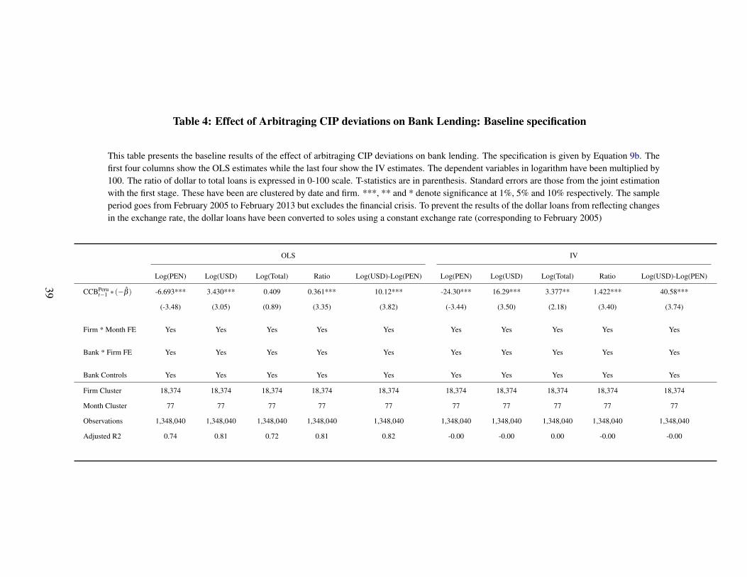
Table 4: Effect of Arbitraging CIP deviations on Bank Lending: Baseline specification

This table presents the baseline results of the effect of arbitraging CIP deviations on bank lending. The specification is given by Equation 9b. Thefirst four columns show the OLS estimates while the last four show the IV estimates. The dependent variables in logarithm have been multiplied by100. The ratio of dollar to total loans is expressed in 0-100 scale. T-statistics are in parenthesis. Standard errors are those from the joint estimationwith the first stage. These have been are clustered by date and firm. ***, ** and * denote significance at 1%, 5% and 10% respectively. The sampleperiod goes from February 2005 to February 2013 but excludes the financial crisis. To prevent the results of the dollar loans from reflecting changesin the exchange rate, the dollar loans have been converted to soles using a constant exchange rate (corresponding to February 2005)

OLS IV

Log(PEN) Log(USD) Log(Total) Ratio Log(USD)-Log(PEN) Log(PEN) Log(USD) Log(Total) Ratio Log(USD)-Log(PEN)

CCBPerut−1 ∗ (−β ) -6.693*** 3.430*** 0.409 0.361*** 10.12*** -24.30*** 16.29*** 3.377** 1.422*** 40.58***

(-3.48) (3.05) (0.89) (3.35) (3.82) (-3.44) (3.50) (2.18) (3.40) (3.74)

Firm * Month FE Yes Yes Yes Yes Yes Yes Yes Yes Yes Yes

Bank * Firm FE Yes Yes Yes Yes Yes Yes Yes Yes Yes Yes

Bank Controls Yes Yes Yes Yes Yes Yes Yes Yes Yes Yes

Firm Cluster 18,374 18,374 18,374 18,374 18,374 18,374 18,374 18,374 18,374 18,374

Month Cluster 77 77 77 77 77 77 77 77 77 77

Observations 1,348,040 1,348,040 1,348,040 1,348,040 1,348,040 1,348,040 1,348,040 1,348,040 1,348,040 1,348,040

Adjusted R2 0.74 0.81 0.72 0.81 0.82 -0.00 -0.00 0.00 -0.00 -0.00

39

ONLINE APPENDIX

40

Table A.I: Summary Statistics of CIP Deviations and FX Changes

This table shows descriptive statistics of the monthly time series of the 1-month cross-currency basis (CCB) forthree groups of currencies between February 2005 and February 2013, excluding the financial crisis. The descriptivestatistics for the USDPEN currency pair are under “Peru”. The cross-currency basis has been computed using midclosing prices reported in Bloomberg (for FX) and mid closing prices of interbank rates in dollar and soles takenfrom the Central Bank of Peru. The descriptive statistics of the average cross-currency basis of four Latin Americancurrency pairs: Brazilian real-dollar (USDBRL), Chilean peso-dollar (USDCLP), Colombian peso-dollar (USDCOP)and Mexican peso-dollar (USDMXN) are under “Av.Latam”, while “Av.Chile, Mexico” contains those pertaining tothe average cross-currency basis of USDCLP and USDMXN. I show this last group because it is the one that hasgreatest correlation with USDPEN. Within each group, the first row, CCB, corresponds to the cross-currency basis,expressed in percentages (on a scale from 0-100). The following two lines describe the summary statistics narrowingthe sample to periods when the basis was either positive or negative. The fourth line shows the absolute value of theCCB. The fifth line shows the 1-month change in CCB in percentage points (pp). This has not been annualized. Thesixth row is analogous but using the absolute value of CCB. Finally, the last row shows the year-over-year changes inthe FX of that currency pair. The last column of this table shows correlations. In the row corresponding to CCB ofeither Av.Latam or Av.Chile and Mexico, it shows the correlation between the CCB of Latam or Chile and Mexico wihthe CCB of Peru. In the row corresponding to the FX, it shows the correlation between the 1-year FX changes and the1-year changes CCB on the corresponding countries.

Mean SD Min Max N ρ

Peru

CCB (%) -0.28 0.74 -2.12 1.98 77.00

CCB > 0 (%) 0.54 0.51 0.08 1.98 24.00

CCB < 0 (%) -0.65 0.49 -2.12 -0.01 53.00

|CCB| (%) 0.62 0.50 0.01 2.12 77.00

∆ 1m CCB (pp) -0.04 0.68 -1.30 2.47 75.00

∆ 1m|CCB| (pp) 0.51 0.45 0.01 2.47 75.00

∆ 12mFX (%) -3.53 3.02 -11.76 4.22 77.00 0.26

Av.Latam

CCB (%) -0.21 0.68 -1.90 1.41 77.00 0.44

CCB > 0 (%) 0.48 0.44 0.00 1.41 28.00

CCB < 0 (%) -0.61 0.42 -1.90 -0.00 49.00

|CCB| (%) 0.56 0.43 0.00 1.90 77.00

∆ 1m CCB (pp) -0.01 0.39 -1.45 1.22 75.00

∆ 1m|CCB| (pp) 0.28 0.27 0.00 1.45 75.00

∆ 12mFX (%) -5.95 6.72 -20.60 8.61 77.00 0.34

Av.Chile, Mexico

CCB (%) -0.03 0.55 -1.47 0.88 77.00 0.54

CCB > 0 (%) 0.40 0.20 0.03 0.88 43.00

CCB < 0 (%) -0.57 0.34 -1.47 -0.01 34.00

|CCB| (%) 0.47 0.28 0.01 1.47 77.00

∆ 1m CCB (pp) 0.00 0.28 -0.63 0.71 75.00

∆ 1m|CCB| (pp) 0.22 0.17 0.01 0.71 75.00

∆ 12mFX (%) -4.81 6.77 -22.00 9.07 77.00 0.30

41

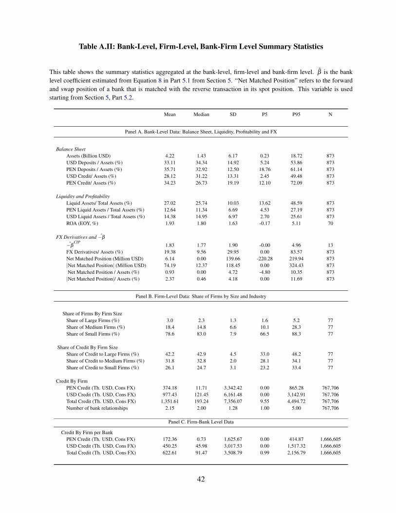
Table A.II: Bank-Level, Firm-Level, Bank-Firm Level Summary Statistics

This table shows the summary statistics aggregated at the bank-level, firm-level and bank-firm level. β is the banklevel coefficient estimated from Equation 8 in Part 5.1 from Section 5. “Net Matched Position” refers to the forwardand swap position of a bank that is matched with the reverse transaction in its spot position. This variable is usedstarting from Section 5, Part 5.2.

Mean Median SD P5 P95 N

Panel A. Bank-Level Data: Balance Sheet, Liquidity, Profitability and FX

Balance SheetAssets (Billion USD) 4.22 1.43 6.17 0.23 18.72 873USD Deposits / Assets (%) 33.11 34.34 14.92 5.24 53.86 873PEN Deposits / Assets (%) 35.71 32.92 12.50 18.76 61.14 873USD Credit/ Assets (%) 28.12 31.22 13.31 2.45 49.48 873PEN Credit/ Assets (%) 34.23 26.73 19.19 12.10 72.09 873

Liquidity and ProfitabilityLiquid Assets/ Total Assets (%) 27.02 25.74 10.03 13.62 48.59 873PEN Liquid Assets / Total Assets (%) 12.64 11.34 6.69 4.53 27.19 873USD Liquid Assets / Total Assets (%) 14.38 14.95 6.97 2.70 25.61 873ROA (EOY, %) 1.93 1.80 1.63 -0.17 5.11 70

FX Derivatives and −β

−βCIP

1.83 1.77 1.90 -0.00 4.96 13FX Derivatives/ Assets (%) 19.38 9.56 29.95 0.00 83.57 873Net Matched Position (Million USD) 6.14 0.00 139.66 -220.28 219.94 873|Net Matched Position| (Million USD) 74.19 12.37 118.45 0.00 324.43 873Net Matched Position / Assets (%) 0.93 0.00 4.72 -4.80 10.35 873|Net Matched Position|/ Assets (%) 2.37 0.46 4.18 0.00 11.69 873

Panel B. Firm-Level Data: Share of Firms by Size and Industry

Share of Firms By Firm SizeShare of Large Firms (%) 3.0 2.3 1.3 1.6 5.2 77Share of Medium Firms (%) 18.4 14.8 6.6 10.1 28.3 77Share of Small Firms (%) 78.6 83.0 7.9 66.5 88.3 77

Share of Credit By Firm SizeShare of Credit to Large Firms (%) 42.2 42.9 4.5 33.0 48.2 77Share of Credit to Medium Firms (%) 31.8 32.8 2.0 28.1 34.1 77Share of Credit to Small Firms (%) 26.1 24.7 3.1 23.2 33.4 77

Credit By FirmPEN Credit (Th. USD, Cons FX) 374.18 11.71 3,342.42 0.00 865.28 767,706USD Credit (Th. USD, Cons FX) 977.43 121.45 6,161.48 0.00 3,142.91 767,706Total Credit (Th. USD, Cons FX) 1,351.61 193.24 7,356.07 9.55 4,494.72 767,706Number of bank relationships 2.15 2.00 1.28 1.00 5.00 767,706

Panel C. Firm-Bank Level Data

Credit By Firm per BankPEN Credit (Th. USD, Cons FX) 172.36 0.73 1,625.67 0.00 414.87 1,666,605USD Credit (Th. USD, Cons FX) 450.25 45.98 3,017.53 0.00 1,517.32 1,666,605Total Credit (Th. USD, Cons FX) 622.61 91.47 3,508.79 0.99 2,156.79 1,666,605

42

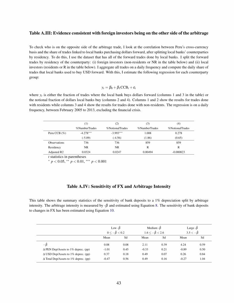
Table A.III: Evidence consistent with foreign investors being on the other side of the arbitrage

To check who is on the opposite side of the arbitrage trade, I look at the correlation between Peru’s cross-currencybasis and the share of trades linked to local banks purchasing dollars forward, after splitting local banks’ counterpartiesby residency. To do this, I use the dataset that has all of the forward trades done by local banks. I split the forwardtrades by residency of the counterparty: (i) foreign investors (non-residents or NR in the table below) and (ii) localinvestors (residents or R in the table below). I aggregate all trades on a daily frequency and compute the daily share oftrades that local banks used to buy USD forward. With this, I estimate the following regression for each counterpartygroup:

yt = β0 +β1CCBt + εt

where yt is either the fraction of trades where the local bank buys dollars forward (columns 1 and 3 in the table) orthe notional fraction of dollars local banks buy (columns 2 and 4). Columns 1 and 2 show the results for trades donewith residents while columns 3 and 4 show the results for trades done with non-residents. The regression is on a dailyfrequency, between February 2005 to 2013, excluding the financial crisis.

(1) (2) (3) (4)

%NumberTrades %NotionalTrades %NumberTrades %NotionalTrades

Peru CCB (%) -4.278∗∗∗ -3.993∗∗∗ 1.008 0.278

(-5.09) (-4.56) (1.86) (0.65)

Observations 736 736 859 859

Residency NR NR R R

Adjusted R2 0.0324 0.0247 0.00494 -0.000823

t statistics in parentheses∗ p < 0.05, ∗∗ p < 0.01, ∗∗∗ p < 0.001

Table A.IV: Sensitivity of FX and Arbitrage Intensity

This table shows the summary statistics of the sensitivity of bank deposits to a 1% depreciation split by arbitrageintensity. The arbitrage intensity is measured by -β and estimated using Equation 8. The sensitivity of bank depositsto changes in FX has been estimated using Equation 10.

Low -β Medium -β Large -β

0≤−β < 0.2 1.6≤−β < 2.6 3.5 <−β

Mean Sd Mean Sd Mean Sd

−β 0.08 0.08 2.11 0.39 4.24 0.59

∆ PEN Dep/Assets to 1% deprec. (pp) -1.01 0.45 -0.33 0.21 -0.89 0.50

∆ USD Dep/Assets to 1% deprec. (pp) 0.37 0.18 0.49 0.07 0.26 0.84

∆ Total Dep/Assets to 1% deprec. (pp) -0.47 0.56 0.49 0.16 -0.27 1.04

43

Table A.V: Baseline results after controlling for FX

This table shows the results of the regression that modifies the baseline regression to add the interaction between log(FX) and the arbitrage intensity (-β ). Allspecifications, unless explicitly noted, use the same fixed effects (firm-month and bank-month fixed effects) and controls (lagged bank controls) as those used inthe baseline specification. The first row shows the baseline coefficients. The dependent variables in logarithm have been multiplied by 100. The ratio of dollar tototal loans is expressed in 0-100 scale. T-statistics are in parenthesis. Standard errors are those from the joint estimation with the first stage. These have been areclustered by date and firm. ***, ** and * denote significance at 1%, 5% and 10% respectively. The sample period goes from February 2005 to February 2013 butexcludes the financial crisis. To prevent the results of the dollar loans from reflecting changes in the exchange rate, the dollar loans have been converted to solesusing a constant exchange rate (corresponding to February 2005).

Log(PEN) Log(USD) Log(Total) Ratio Log(USD)-Log(PEN)

CCBPerut−1 ∗ (−β ) -16.95*** 15.58*** 5.110*** 1.065*** 32.53***

(-2.88) (3.27) (3.05) (2.96) (3.32)

log(FX)t−1 ∗ (−β ) -1.848*** 0.369 -0.138 0.0913*** 2.217***

(-5.03) (1.23) (-1.23) (4.10) (3.75)

Firm * Date FE Yes Yes Yes Yes Yes

Bank * Firm FE Yes Yes Yes Yes Yes

Bank Controls Yes Yes Yes Yes Yes

Firm Cluster 17,113 17,113 17,113 17,113 17,113

Month Cluster 75 75 75 75 75

Observations 1,241,908 1,241,908 1,241,908 1,241,908 1,241,908

Adjusted R2 0.00 -0.00 0.00 0.00 -0.00

44

Table A.VI: Effect of Arbitraging CIP deviations on Bank Lending: Alternative Samples

This table shows robustness checks under different samples. All specifications, unless explicitly noted, use the same fixed effects (firm-month andbank-month fixed effects) and controls (lagged bank controls) as those used in the baseline specification. The dependent variables in logarithmhave been multiplied by 100. The ratio of dollar to total loans is expressed in 0-100 scale. The first row shows the baseline coefficients. Thefirst five columns show the second stage IV coefficients of the baseline specification (i.e. with lagged bank controls, bank-firm and month-firmfixed effects) under different samples. The last three columns show other statistics (number of observations, number of firm clusters and numberof month clusters). The first row shows the baseline second-stage regression shown in Table 4. The second row restricts the sample to the largestfour banks. The third sample restricts the sample to those firms without foreign trade. The fourth row restricts the sample to to commercial loansonly. To do so, I started with the loan-level dataset instead of the dataset that aggregated loans at the bank-firm-month level. The dataset aggregatedat the bank-firm-month level was used for the other regressions. Finally, the last line shows the coefficients for all the financial system. All theprevious regressions were only for banks. Other financial institutions include financials and cajas. These are subject to different banking regulationthan banks. T-statistics are in parenthesis. Standard errors are those from the joint estimation with the first stage. These have been are clustered bydate and firm. ***, ** and * denote significance at 1%, 5% and 10% respectively. The sample period goes from February 2005 to February 2013but excludes the financial crisis. To prevent the results of the dollar loans from reflecting changes in the exchange rate, the dollar loans have beenconverted to soles using a constant exchange rate (corresponding to February 2005).

Estimates Other Stats

Log(PEN) Log(USD) Log(Total) Ratio Log(USD)-Log(PEN) Obs Firm Cl. Month Cl.

(1) Baseline -24.30*** 16.29*** 3.38** 1.42*** 40.58*** 1,348,040.00 18,374.00 77.00

(-3.44) (3.50) (2.18) (3.40) (3.74)

(2) Largest Banks Only -36.62*** 40.93*** 8.53*** 3.23*** 77.55*** 1,056,886.00 16,849.00 77.00

(-3.27) (4.15) (2.99) (3.84) (3.92)

(3) Without Foreign Trade Firms -19.37*** 15.16*** 0.68 1.35*** 34.53*** 865,066.00 14,820.00 77.00

(-3.02) (2.81) (0.39) (2.88) (3.24)

(4) Commercial Loans Only -28.11*** 20.03*** -0.24 2.05*** 48.13*** 669,351.00 12,415.00 77.00

(-3.27) (2.88) (-0.14) (3.29) (3.27)

(5) Borrowing USD and PEN -6.02* 5.21* 0.50 0.89** 11.23** 280,282.00 6,189.00 77.00

(-1.83) (1.82) (0.32) (2.02) (2.41)

(6) All financial institutions -17.48*** 11.55*** 3.80** 0.97*** 29.03*** 1,438,071.00 19,054.00 77.00

(-3.01) (3.14) (2.52) (2.92) (3.40)

45

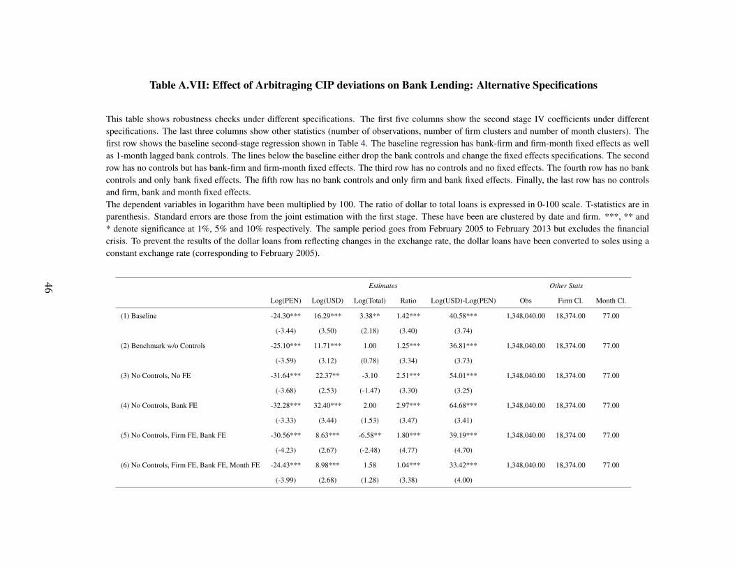
Table A.VII: Effect of Arbitraging CIP deviations on Bank Lending: Alternative Specifications

This table shows robustness checks under different specifications. The first five columns show the second stage IV coefficients under differentspecifications. The last three columns show other statistics (number of observations, number of firm clusters and number of month clusters). Thefirst row shows the baseline second-stage regression shown in Table 4. The baseline regression has bank-firm and firm-month fixed effects as wellas 1-month lagged bank controls. The lines below the baseline either drop the bank controls and change the fixed effects specifications. The secondrow has no controls but has bank-firm and firm-month fixed effects. The third row has no controls and no fixed effects. The fourth row has no bankcontrols and only bank fixed effects. The fifth row has no bank controls and only firm and bank fixed effects. Finally, the last row has no controlsand firm, bank and month fixed effects.The dependent variables in logarithm have been multiplied by 100. The ratio of dollar to total loans is expressed in 0-100 scale. T-statistics are inparenthesis. Standard errors are those from the joint estimation with the first stage. These have been are clustered by date and firm. ***, ** and* denote significance at 1%, 5% and 10% respectively. The sample period goes from February 2005 to February 2013 but excludes the financialcrisis. To prevent the results of the dollar loans from reflecting changes in the exchange rate, the dollar loans have been converted to soles using aconstant exchange rate (corresponding to February 2005).

Estimates Other Stats

Log(PEN) Log(USD) Log(Total) Ratio Log(USD)-Log(PEN) Obs Firm Cl. Month Cl.

(1) Baseline -24.30*** 16.29*** 3.38** 1.42*** 40.58*** 1,348,040.00 18,374.00 77.00

(-3.44) (3.50) (2.18) (3.40) (3.74)

(2) Benchmark w/o Controls -25.10*** 11.71*** 1.00 1.25*** 36.81*** 1,348,040.00 18,374.00 77.00

(-3.59) (3.12) (0.78) (3.34) (3.73)

(3) No Controls, No FE -31.64*** 22.37** -3.10 2.51*** 54.01*** 1,348,040.00 18,374.00 77.00

(-3.68) (2.53) (-1.47) (3.30) (3.25)

(4) No Controls, Bank FE -32.28*** 32.40*** 2.00 2.97*** 64.68*** 1,348,040.00 18,374.00 77.00

(-3.33) (3.44) (1.53) (3.47) (3.41)

(5) No Controls, Firm FE, Bank FE -30.56*** 8.63*** -6.58** 1.80*** 39.19*** 1,348,040.00 18,374.00 77.00

(-4.23) (2.67) (-2.48) (4.77) (4.70)

(6) No Controls, Firm FE, Bank FE, Month FE -24.43*** 8.98*** 1.58 1.04*** 33.42*** 1,348,040.00 18,374.00 77.00

(-3.99) (2.68) (1.28) (3.38) (4.00)

46

Table A.VIII: Effect of Arbitraging CIP deviations on Bank Lending: Alternative Computations of CIP Deviations

This table shows the second stage results for the baseline regression when computing the alternative versions of the cross-currency basis. Allspecifications, unless explicitly noted, use the same fixed effects (firm-month and bank-month fixed effects) and controls (lagged bank controls)as those used in the baseline specification. The first row shows the baseline coefficients. The second row shows the coefficients when computingCIP deviations using bid-ask spreads for all of these prices, both for the USDPEN basis as well as the USDCLP and USDMXN basis used as IV.The third row computes the cross-currency basis using dollar Libor rates instead of the dollar interbank rate. Finally, the last row computes thecross-currency using the inferred put-call parity relationship rates from van Binsberger, Diamond, and Grotteria (2021). The dependent variablesin logarithm have been multiplied by 100. The ratio of dollar to total loans is expressed in 0-100 scale. T-statistics are in in parenthesis. Standarderrors are those from the joint estimation with the first stage. These have been are clustered by date and firm. ***, ** and * denote significanceat 1%, 5% and 10% respectively. The sample period goes from February 2005 to February 2013 but excludes the financial crisis. To prevent theresults of the dollar loans from reflecting changes in the exchange rate, the dollar loans have been converted to soles using a constant exchange rate(corresponding to February 2005).

Estimates Other Stats

Log(PEN) Log(USD) Log(Total) Ratio Log(USD)-Log(PEN) Obs Firm Cl. Month Cl.

(1) Baseline -24.30*** 16.29*** 3.38** 1.42*** 40.58*** 1,348,040.00 18,374.00 77.00

(-3.44) (3.50) (2.18) (3.40) (3.74)

(2) CCB With Bid-Ask Spreads -31.74** 27.27** 7.02 1.92** 59.01** 1,348,040.00 18,374.00 77.00

(-2.09) (2.00) (1.61) (2.05) (2.12)

(3) CCB Using Libor Rates -46.83* 34.43** 8.38* 2.85* 81.26** 1,348,040.00 18,374.00 77.00

(-1.98) (1.99) (1.81) (1.95) (2.03)

(4) CCB Using vBDG -43.95** 33.12** 8.41* 2.68** 77.08** 1,348,040.00 18,374.00 77.00

(-2.03) (2.06) (1.86) (2.00) (2.09)

47

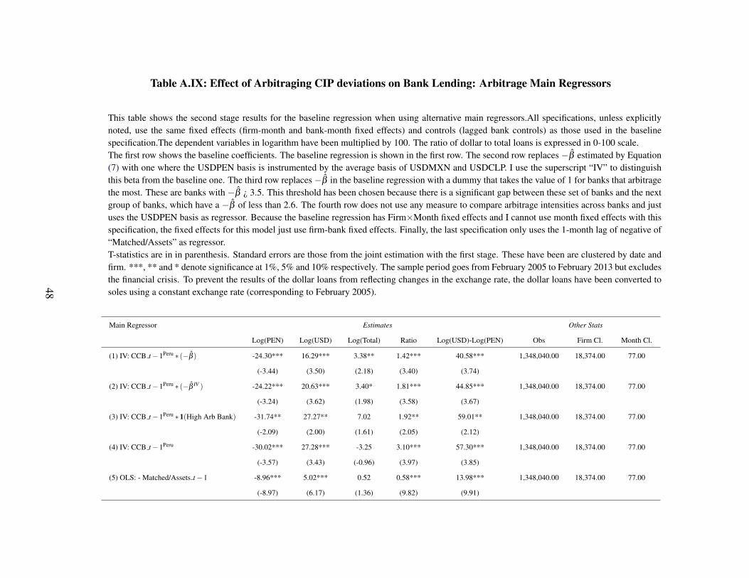
Table A.IX: Effect of Arbitraging CIP deviations on Bank Lending: Arbitrage Main Regressors

This table shows the second stage results for the baseline regression when using alternative main regressors.All specifications, unless explicitlynoted, use the same fixed effects (firm-month and bank-month fixed effects) and controls (lagged bank controls) as those used in the baselinespecification.The dependent variables in logarithm have been multiplied by 100. The ratio of dollar to total loans is expressed in 0-100 scale.The first row shows the baseline coefficients. The baseline regression is shown in the first row. The second row replaces −β estimated by Equation(7) with one where the USDPEN basis is instrumented by the average basis of USDMXN and USDCLP. I use the superscript “IV” to distinguishthis beta from the baseline one. The third row replaces−β in the baseline regression with a dummy that takes the value of 1 for banks that arbitragethe most. These are banks with −β ¿ 3.5. This threshold has been chosen because there is a significant gap between these set of banks and the nextgroup of banks, which have a −β of less than 2.6. The fourth row does not use any measure to compare arbitrage intensities across banks and justuses the USDPEN basis as regressor. Because the baseline regression has Firm×Month fixed effects and I cannot use month fixed effects with thisspecification, the fixed effects for this model just use firm-bank fixed effects. Finally, the last specification only uses the 1-month lag of negative of“Matched/Assets” as regressor.T-statistics are in in parenthesis. Standard errors are those from the joint estimation with the first stage. These have been are clustered by date andfirm. ***, ** and * denote significance at 1%, 5% and 10% respectively. The sample period goes from February 2005 to February 2013 but excludesthe financial crisis. To prevent the results of the dollar loans from reflecting changes in the exchange rate, the dollar loans have been converted tosoles using a constant exchange rate (corresponding to February 2005).

Main Regressor Estimates Other Stats

Log(PEN) Log(USD) Log(Total) Ratio Log(USD)-Log(PEN) Obs Firm Cl. Month Cl.

(1) IV: CCB t−1Peru ∗ (−β ) -24.30*** 16.29*** 3.38** 1.42*** 40.58*** 1,348,040.00 18,374.00 77.00

(-3.44) (3.50) (2.18) (3.40) (3.74)

(2) IV: CCB t−1Peru ∗ (−β IV ) -24.22*** 20.63*** 3.40* 1.81*** 44.85*** 1,348,040.00 18,374.00 77.00

(-3.24) (3.62) (1.98) (3.58) (3.67)

(3) IV: CCB t−1Peru ∗1(High Arb Bank) -31.74** 27.27** 7.02 1.92** 59.01** 1,348,040.00 18,374.00 77.00

(-2.09) (2.00) (1.61) (2.05) (2.12)

(4) IV: CCB t−1Peru -30.02*** 27.28*** -3.25 3.10*** 57.30*** 1,348,040.00 18,374.00 77.00

(-3.57) (3.43) (-0.96) (3.97) (3.85)

(5) OLS: - Matched/Assets t−1 -8.96*** 5.02*** 0.52 0.58*** 13.98*** 1,348,040.00 18,374.00 77.00

(-8.97) (6.17) (1.36) (9.82) (9.91)

48

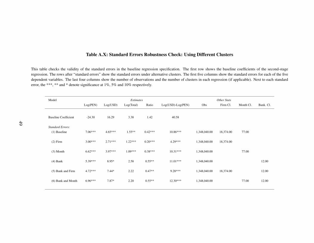
Table A.X: Standard Errors Robustness Check: Using Different Clusters

This table checks the validity of the standard errors in the baseline regression specification. The first row shows the baseline coefficients of the second-stageregression. The rows after “standard errors” show the standard errors under alternative clusters. The first five columns show the standard errors for each of the fivedependent variables. The last four columns show the number of observations and the number of clusters in each regression (if applicable). Next to each standarderror, the ***, ** and * denote significance at 1%, 5% and 10% respectively.

Model Estimates Other Stats

Log(PEN) Log(USD) Log(Total) Ratio Log(USD)-Log(PEN) Obs Firm Cl. Month Cl. Bank. Cl.

Baseline Coefficient -24.30 16.29 3.38 1.42 40.58

Standard Errors:

(1) Baseline 7.06*** 4.65*** 1.55** 0.42*** 10.86*** 1,348,040.00 18,374.00 77.00

(2) Firm 3.00*** 2.71*** 1.22*** 0.20*** 4.29*** 1,348,040.00 18,374.00

(3) Month 6.62*** 3.97*** 1.09*** 0.38*** 10.31*** 1,348,040.00 77.00

(4) Bank 5.39*** 8.95* 2.58 0.55** 11.01*** 1,348,040.00 12.00

(5) Bank and Firm 4.72*** 7.44* 2.22 0.47** 9.28*** 1,348,040.00 18,374.00 12.00

(6) Bank and Month 6.96*** 7.87* 2.20 0.55** 12.30*** 1,348,040.00 77.00 12.00

49

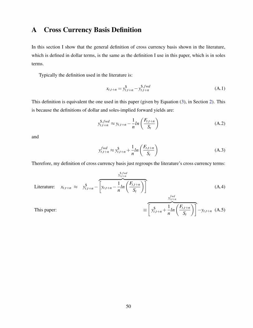
A Cross Currency Basis Definition

In this section I show that the general definition of cross currency basis shown in the literature,

which is defined in dollar terms, is the same as the definition I use in this paper, which is in soles

terms.

Typically the definition used in the literature is:

xt,t+n = y$t,t+n− y$, f wd

t,t+n (A.1)

This definition is equivalent the one used in this paper (given by Equation (3), in Section 2). This

is because the definitions of dollar and soles-implied forward yields are:

y$, f wdt,t+n ≈ yt,t+n−

1n

ln(

Ft,t+n

St

)(A.2)

and

y f wdt,t+n ≈ y$

t,t+n +1n

ln(

Ft,t+n

St

)(A.3)

Therefore, my definition of cross currency basis just regroups the literature’s cross currency terms:

Literature: xt,t+n ≈ y$t,t+n−

y$, f wdt,t+n︷ ︸︸ ︷[

yt,t+n−1n

ln(

Ft,t+n

St

)](A.4)

This paper: ≡

y f wdt,t+n︷ ︸︸ ︷[

y$t,t+n +

1n

ln(

Ft,t+n

St

)]−yt,t+n (A.5)

50

B Possible explanations for the differences in the cross-currencybasis of developed and developing economies

Explanations for the differences between developed and developing economies possibly stem from

differences in the degree of market segmentation in the transactions required to arbitrage and the

sources of dollar liquidity.

Market segmentation. The degree of market segmentation in FX and money markets differs

between developed and developing economies. Two important factors affect market segmentation

in developing economies: (i) capital controls and (ii) delivery of local currency.

Between 2010-2012, various developing countries set capital controls on inflows to limit carry

trade inflows. These controls typically involve a series of regulations that affect money markets

as well as the forward markets. In the money market, regulations have included high reserve

requirements when local banks borrow dollars short-term from abroad, as well as fees when

foreign investors would buy short-term local currency debt. In the forward market, regulations

have included restrictions for local banks when purchasing dollars from abroad.

In Peru, capital controls on inflows were imposed starting in 2008 and then reinforced in 2011

(see Keller (2020) for a detailed analysis of these controls). A first set of regulation imposed

in 2008 included high reserve requirements when local banks borrowed dollars from abroad, as

well as high fees for foreign investors when purchasing soles certificates of deposit from the

Central Bank. A second set of regulation imposed in 2011 set limits on forward holdings of local

banks. These restrictions segment money markets and FX markets between foreign investors and

local banks that can partially explain part of the cross-currency basis in Peru and other emerging

economies with similar regulations.

Besides capital controls, the delivery of local currency is also an aspect that naturally segments

foreign investors from local banks. Typically, emerging market currencies cannot be delivered

abroad. This means that for foreign banks to trade FX spot, which is deliverable, they typically

need a current account in the emerging economy. This means that foreign investors trade mostly

non-delivery forward contracts. This is the case in Peru where, 85% of trades in my sample are

51

non-delivery forwards (NDF).34 Therefore, large changes in foreigners’ demand for dollars in the

forward market could create an additional pressure in the forward market. In contrast to this, local

banks trade both in the forward and in the spot market and therefore have an advantage when

arbitraging CIP deviations.

More generally, there are other factors that affect market segmentation that are present in

developed and developing economies. In both cases, local banks usually have an advantage when

borrowing and investing in the local currency because they are the authorized agents to participate

in auctions from the central bank.

Sources of dollar liquidity. Because of past instability and hyperinflation, various emerging

economies are partially dollarized. This means that there is already dollar liquidity in the country.

Factors affecting such liquidity included FX interventions from the Peruvian Central bank. Clearly,

these factors are not present in developed economies.

34This means that only the net profit is exchanged at the end of the forward contract and this is settled in dollars.Indeed, confidential daily FX spot data that banks report to the Central Bank, shows that foreign investors do not tradespot FX. Forward transactions of banks, however, show that 90% of foreign investors’ forward trades are NDF.

52