
Arbitrage-Free Pricing Of Derivatives In Nonlinear Market ...
42
Arbitrage-Free Pricing Of Derivatives In Nonlinear Market Models Tomasz R. Bielecki a , Igor Cialenco a , and Marek Rutkowski b First Circulated: January 28, 2017 Abstract: The main objective is to study no-arbitrage pricing of financial derivatives in the pres- ence of funding costs, the counterparty credit risk and market frictions affecting the trading mechanism, such as collateralization and capital requirements. To achieve our goals, we extend in several respects the nonlinear pricing approach developed in El Karoui and Quenez [EKQ97] and El Karoui et al. [EKPQ97]. Keywords: hedging, fair price, funding cost, margin agreement, market friction, BSDE MSC2010: 91G40, 60J28 Contents 1 Introduction 3 2 Nonlinear Market Model 4 2.1 Contracts with Trading Adjustments ........................... 4 2.2 Self-financing Trading Strategies ............................. 5 2.3 Funding Adjustment .................................... 7 2.4 Financial Interpretation of Trading Adjustments .................... 8 2.5 Wealth Process ....................................... 9 2.6 Trading in Risky Assets .................................. 10 2.6.1 Cash Market Trading ............................... 10 2.6.2 Short Selling of Risky Assets ........................... 11 2.6.3 Repo Market Trading ............................... 11 2.7 Collateralization ...................................... 12 2.7.1 Rehypothecated Collateral ............................. 13 2.7.2 Segregated Collateral ............................... 13 2.7.3 Initial and Variation Margins ........................... 14 2.8 Counterparty Credit Risk ................................. 14 2.8.1 Closeout Payoff ................................... 14 2.8.2 Counterparty Credit Risk Decomposition .................... 15 2.9 Regulatory Capital ..................................... 17 a Department of Applied Mathematics, Illinois Institute of Technology 10 W 32nd Str, Building E1, Room 208, Chicago, IL 60616, USA Emails: [email protected] (T.R. Bielecki) and [email protected] (I. Cialenco) URLs: http://math.iit.edu/ ~ bielecki and http://math.iit.edu/ ~ igor b School of Mathematics and Statistics, University of Sydney, Sydney, NSW 2006, Australia and Faculty of Mathematics and Information Science, Warsaw University of Technology, 00-661 Warszawa, Poland Email: [email protected], URL: http://sydney.edu.au/science/people/marek.rutkowski.php 1
Transcript of Arbitrage-Free Pricing Of Derivatives In Nonlinear Market ...
Arbitrage-Free Pricing Of Derivatives In Nonlinear Market Models
Tomasz R. Bielecki a, Igor Cialenco a, and Marek Rutkowski b
First Circulated: January 28, 2017
Abstract: The main objective is to study no-arbitrage pricing of financial derivatives in the pres-ence of funding costs, the counterparty credit risk and market frictions affecting thetrading mechanism, such as collateralization and capital requirements. To achieve ourgoals, we extend in several respects the nonlinear pricing approach developed in ElKaroui and Quenez [EKQ97] and El Karoui et al. [EKPQ97].
Keywords: hedging, fair price, funding cost, margin agreement, market friction, BSDEMSC2010: 91G40, 60J28
Contents
1 Introduction 3
2 Nonlinear Market Model 4
2.1 Contracts with Trading Adjustments . . . . . . . . . . . . . . . . . . . . . . . . . . . 4
2.2 Self-financing Trading Strategies . . . . . . . . . . . . . . . . . . . . . . . . . . . . . 5
2.3 Funding Adjustment . . . . . . . . . . . . . . . . . . . . . . . . . . . . . . . . . . . . 7
2.4 Financial Interpretation of Trading Adjustments . . . . . . . . . . . . . . . . . . . . 8
2.5 Wealth Process . . . . . . . . . . . . . . . . . . . . . . . . . . . . . . . . . . . . . . . 9
2.6 Trading in Risky Assets . . . . . . . . . . . . . . . . . . . . . . . . . . . . . . . . . . 10
2.6.1 Cash Market Trading . . . . . . . . . . . . . . . . . . . . . . . . . . . . . . . 10
2.6.2 Short Selling of Risky Assets . . . . . . . . . . . . . . . . . . . . . . . . . . . 11
2.6.3 Repo Market Trading . . . . . . . . . . . . . . . . . . . . . . . . . . . . . . . 11
2.7 Collateralization . . . . . . . . . . . . . . . . . . . . . . . . . . . . . . . . . . . . . . 12
2.7.1 Rehypothecated Collateral . . . . . . . . . . . . . . . . . . . . . . . . . . . . . 13
2.7.2 Segregated Collateral . . . . . . . . . . . . . . . . . . . . . . . . . . . . . . . 13
2.7.3 Initial and Variation Margins . . . . . . . . . . . . . . . . . . . . . . . . . . . 14
2.8 Counterparty Credit Risk . . . . . . . . . . . . . . . . . . . . . . . . . . . . . . . . . 14
2.8.1 Closeout Payoff . . . . . . . . . . . . . . . . . . . . . . . . . . . . . . . . . . . 14
2.8.2 Counterparty Credit Risk Decomposition . . . . . . . . . . . . . . . . . . . . 15
2.9 Regulatory Capital . . . . . . . . . . . . . . . . . . . . . . . . . . . . . . . . . . . . . 17
aDepartment of Applied Mathematics, Illinois Institute of Technology10 W 32nd Str, Building E1, Room 208, Chicago, IL 60616, USAEmails: [email protected] (T.R. Bielecki) and [email protected] (I. Cialenco)URLs: http://math.iit.edu/~bielecki and http://math.iit.edu/~igor
bSchool of Mathematics and Statistics, University of Sydney, Sydney, NSW 2006, Australiaand Faculty of Mathematics and Information Science, Warsaw University of Technology, 00-661 Warszawa, PolandEmail: [email protected], URL: http://sydney.edu.au/science/people/marek.rutkowski.php
1

2 T.R. Bielecki, I. Cialenco and M. Rutkowski
3 Arbitrage-Free Trading Models 173.1 No-arbitrage Pricing Principles . . . . . . . . . . . . . . . . . . . . . . . . . . . . . . 173.2 Discounted Wealth and Admissible Strategies . . . . . . . . . . . . . . . . . . . . . . 183.3 No-arbitrage with Respect to the Null Contract . . . . . . . . . . . . . . . . . . . . . 193.4 No-arbitrage for the Trading Desk . . . . . . . . . . . . . . . . . . . . . . . . . . . . 203.5 Dynamics of the Discounted Wealth Process . . . . . . . . . . . . . . . . . . . . . . . 223.6 Sufficient Conditions for the Trading Desk No-Arbitrage . . . . . . . . . . . . . . . . 23
4 Hedger’s Fair Pricing 244.1 Replication on [0, T ] and the Gained Value . . . . . . . . . . . . . . . . . . . . . . . 264.2 Market Regularity on [0, T ] . . . . . . . . . . . . . . . . . . . . . . . . . . . . . . . . 26
4.2.1 Replicable Contracts . . . . . . . . . . . . . . . . . . . . . . . . . . . . . . . . 284.2.2 Non-replicable Contracts . . . . . . . . . . . . . . . . . . . . . . . . . . . . . 28
5 Pricing in Regular Models 285.1 Replication and Market Regularity on [t, T ] . . . . . . . . . . . . . . . . . . . . . . . 295.2 Hedger’s Ex-dividend Price at Time t . . . . . . . . . . . . . . . . . . . . . . . . . . 305.3 Marked-to-Market Value . . . . . . . . . . . . . . . . . . . . . . . . . . . . . . . . . . 315.4 Offsetting Price . . . . . . . . . . . . . . . . . . . . . . . . . . . . . . . . . . . . . . . 32
6 A BSDE Approach to Nonlinear Pricing 326.1 BSDE for the Gained Value . . . . . . . . . . . . . . . . . . . . . . . . . . . . . . . . 336.2 BSDE for the Ex-dividend Price . . . . . . . . . . . . . . . . . . . . . . . . . . . . . 356.3 BSDE for the CCR Price . . . . . . . . . . . . . . . . . . . . . . . . . . . . . . . . . 36
7 Appendix: Examples of Non-Regular Models 407.1 Model with Trading Constraints . . . . . . . . . . . . . . . . . . . . . . . . . . . . . 407.2 Model Without Trading Constraints . . . . . . . . . . . . . . . . . . . . . . . . . . . 41
8 Appendix: Local and Global Pricing Problems 42
Derivatives Pricing in Nonlinear Models 3
1 Introduction
The present work contributes to the nonlinear pricing theory, which arises in a natural way whenaccounting for salient features of real-world trades such as: trading constraints, differential fundingcosts, collateralization, counterparty credit risk and capital requirements. To be more specific, theaim of our study is to extend in several respects the hedging and pricing approach in nonlinearmarket models developed in El Karoui and Quenez [EKQ97] and El Karoui et al. [EKPQ97] (seealso [CK93, DQS14, DQS15, KK96, KK98] for hedging and pricing with constrained portfolios)by accounting for the complexity of over-the-counter financial derivatives and specific featuresof the trading environment after the global financial crisis. Let us briefly summarize the maincontributions of this work:
• The first goal is to discuss the trading strategies in the presence of differential funding ratesand adjustment processes. We stress that the need for a more general approach arises due tothe fact that we study general contracts with cash flow streams, rather than simple contingentclaims with a single payoff at maturity (or upon exercise).
• Second, we examine in detail the issues of the existence of arbitrage opportunities for thehedger and for the trading desk in a nonlinear trading framework and with respect to apredetermined class of contracts. We introduce the concept of no-arbitrage with respect tothe null contract and a stronger notion of no-arbitrage for the trading desk. We then proceedto the issue of unilateral fair valuation of a given contract by the hedger endowed with aninitial capital. We examine the link between the concept of no-arbitrage for the trading deskand the financial viability of prices computed by the hedger.
• Third, we propose and analyze the concept of a regular market model, which extends theconcept of a nonlinear pricing system introduced in El Karoui and Quenez [EKQ97]. Thegoal is to identify a class of nonlinear market models, which are arbitrage-free for the tradingdesk and, in addition, enjoy the desirable property that for contracts that can be replicated,the cost of replication is also the fair price for the hedger.
• Next, we focus on replication of a contract in a regular market model and we discuss the BSDEapproach to the valuation and hedging of contracts in a model with differential funding rates,the counterparty credit risk and trading adjustments. We propose two main definitions ofno-arbitrage prices, namely, the gained value and the ex-dividend price, and we show thatthey in fact coincide, under suitable technical conditions, when the pricing problem underconsideration is local. It is worth stressing that in the case of a global pricing problem thetwo above-mentioned definitions will typically yield different pricing results for the hedger.To complete our study, we also examine the marked-to-market valuation of a contract andthe problem of unwinding and offsetting for an existing contract.
• We conclude the paper by briefly addressing the issue of fair valuation and hedging of acounterparty risky contract in a nonlinear market model.
It should be acknowledged that we focus on fair unilateral pricing from the perspective of thehedger, although it is clear that the same definitions and pricing methods are applicable to hiscounterparty as well. Hence, in principle, it is also possible to use our results in order to examinethe interval of fair bilateral prices in a regular market model. Particular instances of bilateral pricingproblems were studied in [NR15, NR16a, NR16c] where it was shown that a non-empty interval offair bilateral prices (or bilaterally profitable prices) can be obtained in some nonlinear models for

4 T.R. Bielecki, I. Cialenco and M. Rutkowski
contracts with either an exogenous or an endogenous collateralization. For more practical studies ofpricing and hedging subject to differential funding costs and the counterparty credit risk to whichour general theory can be applied, the reader is referred to [BCS15, BP14, BK11, BK13, Cre15a,Cre15b, PPB12a, PPB12b, Pit10].
2 Nonlinear Market Model
In this section, we extend a generic market model introduced in [BR15]. Throughout the paper,we fix a finite trading horizon date T > 0 for our model of the financial market. Let (Ω,G,G,P)be a filtered probability space satisfying the usual conditions of right-continuity and completeness,where the filtration G = (Gt)t∈[0,T ] models the flow of information available to all traders. Forconvenience, we assume that the initial σ-field G0 is trivial. Moreover, all processes introduced inwhat follows are implicitly assumed to be G-adapted and, as usual, any semimartingale is assumedto be cadlag. Also, we will assume that any process Y satisfies ∆Y0 := Y0 − Y0− = 0. Let usintroduce the notation for the prices of all traded assets in our model.
Risky assets. We denote by S = (S1, . . . , Sd) the collection of the ex-dividend prices of a family ofd risky assets with the corresponding cumulative dividend streams D = (D1, . . . , Dd). The processSi is aimed to represent the ex-dividend price of any traded security, such as, stock, sovereign orcorporate bond, stock option, interest rate swap, currency option or swap, CDS, CDO, etc.
Cash accounts. The lending cash account B0,l and the borrowing cash account B0,b are used forunsecured lending and borrowing of cash, respectively. For brevity, we will sometimes write Bl andBb instead of B0,l and B0,b. Also, when the borrowing and lending cash rates are equal, the singlecash account is denoted by B0 or simply B.
Funding accounts. We denote by Bi,l (resp. Bi,b) the lending (resp. borrowing) funding accountassociated with the ith risky asset, for i = 1, 2, . . . , d. The financial interpretation of these accountsvaries from case to case. For an overview of trading mechanisms for risky assets, we refer to toSection 2.6. In the special case when Bi,l = Bi,b, we will use the notation Bi and we call it thefunding account for the ith risky asset.
For brevity, denote by B = ((Bi,l, Bi,b), i = 0, 1, . . . , d) the collection of all cash and fundingaccounts.
2.1 Contracts with Trading Adjustments
We will consider financial contracts between two parties, called the hedger and the counterparty.In what follows, all the cash flows will be viewed from the prospective of the hedger. A bilateralfinancial contract (or simply a contract) is given as a pair C = (A,X ) where the meaning of eachterm is explained below.
A stochastic processes A represents the cumulative cash flows from time 0 till maturity date T .The process A is assumed to model the (cumulative) cash flows of a given contract, which are eitherpaid out from the hedger’s wealth or added to the his wealth via the value process of his portfolioof traded assets (including cash). Note that the price of the contract exchanged at its initiationwill not be included in A. For example, if a contract stipulates that the hedger will ‘receive’ the(possibly random) cash flows a1, a2, . . . , am at times t1, t2, . . . , tm ∈ (0, T ], then
At =m∑l=1
1[tl,∞)(t)al.

Derivatives Pricing in Nonlinear Models 5
Let (At, 0) denote a contract initiated at time t with X = 0. Then the only cash flow exchangedbetween parties at time t is the price of the contract, denoted as pt, and thus the remaining cashflows of (At, 0) are given as Atu := Au −At for u ∈ [t, T ]. In particular, the equality Att = 0 is validfor any contract (A, 0) and any date t ∈ [0, T ). All future cash flows al for l such that tl > t arepredetermined, in the sense that they are explicitly specified by the contract covenants, but theprice pt needs to be first properly defined and next computed using some particular market model.
As an example, consider the situation where the hedger sells at time t a European call optionon the risky asset Si. Then m = 1, t1 = T , and the terminal payoff from the perspective ofthe issuer equals a1 = −(SiT − K)+. Consequently, for every t ∈ [0, T ), the process At satisfiesAtu = −(SiT −K)+1[T,∞)(u) for all u ∈ [t, T ]. Obviously, the price pt of the option depends bothon a market model and a pricing method.
To account for market frictions, we postulate that the cash flows A (resp. At) of a contractare complemented by trading adjustments, which are formally represented by the process X (resp.X t) given as X = (X1, . . . , Xn;α1, . . . , αn;β1, . . . , βn). Its role is to describe additional tradingcovenants associated with a given contract, such as collateralization and regulatory capital, aswell as the adjustments due to the counterparty credit risk. For each adjustment process Xk,the auxiliary process αkXk represents additional incoming or outgoing cash flows for the hedger,which are either stipulated in the clauses of a contract (e.g., the credit support annex) or imposedby a third party (for instance, the regulator). In addition, each process Xk, k = 1, 2, . . . , nis complemented by the corresponding remuneration process βk, which is used to determine netinterest payments (if any) associated with the process Xk. It should be noted that the processesX1, . . . , Xn and the associated remuneration processes β1, . . . , βn do not represent traded assets.It is rather clear that the processes α and β may depend on the respective adjustment process.Therefore, when the adjustment process is Y, rather than X , one should write α(Y) and β(Y) inorder to avoid confusion. However, for brevity, we will keep the shorthand notation α and β whenthe adjustment process is denoted as X .
Valuation or pricing of a given contract means, in particular, to find the range of fair pricespt at any date t from the viewpoint of either the hedger or the counterparty. Although it will bepostulated that both parties adopt the same valuation paradigm, due to the asymmetry of cashflows, differential trading costs and possibly also different trading opportunities, they will typicallyobtain different ranges for fair unilateral prices for a given bilateral contract. The discrepancy inpricing for the two parties is a consequence of the nonlinearity of the wealth dynamics in tradingstrategies, so that it may occur even within the framework a complete market model where theperfect replication of any contract can be achieved by both parties.
2.2 Self-financing Trading Strategies
The concept of a portfolio refers to the family of primary traded assets, that is, risky assets, cashaccounts, and funding accounts for risky assets. Formally, by a portfolio on the time interval [t, T ],we mean an arbitrary R3d+2-valued, G-adapted process (ϕtu)u∈[t,T ] denoted as
ϕt =(ξ1, . . . , ξd;ψ0,l, ψ0,b, ψ1,l, ψ1,b, . . . , ψd,l, ψd,b
)(2.1)
where the components represent positions in risky assets (Si, Di), i = 1, 2, . . . , d, cash accountsB0,l, B0,b, and funding accountsBi,l, Bi,b, i = 1, 2, . . . , d for risky assets. It is postulated throughoutthat ψj,lu ≥ 0, ψj,bu ≤ 0 and ψj,lu ψ
j,bu = 0 for all j = 0, 1, . . . , d and u ∈ [t, T ]. If the borrowing and
lending rates are equal, then we denote by Bj , for j = 0, 1, . . . , d, the corresponding cash or fundingaccount and we denote ψj = ψj,l +ψj,b. It is also assumed throughout that the processes ξ1, . . . , ξd
are G-predictable.

6 T.R. Bielecki, I. Cialenco and M. Rutkowski
We say that a portfolio ϕ is constrained if at least one of the components of the process ϕ isassumed to satisfy some additional constraints. For instance, we will need to impose conditionsensuring that the funding of each risky asset is done using the corresponding funding account.Another example of an explicit constraint is obtained when we set ψ0,b
u = 0 for all u ∈ [t, T ],meaning that an outright borrowing of cash from the account B0,b is prohibited. We are now in aposition to state some fairly standard technical assumptions underpinning our further developments.
Assumption 2.1. We work throughout under the following standing assumptions:
(i) for every i = 1, 2, . . . , d, the price Si of the ith risky asset is a semimartingale and thecumulative dividend stream Di is a process of finite variation with Di
0 = 0;
(ii) the cash and funding accounts Bj,l and Bj,b are strictly positive and continuous processes of
finite variation with Bj,l0 = Bj,b
0 = 1 for j = 0, 1, . . . , d;
(iii) the cumulative cash flow process A of any contract is a process of finite variation;
(iv) the adjustment processes Xk, k = 1, 2, . . . , n and the auxiliary processes αk, k = 1, 2, . . . , nare semimartingales;
(v) the remuneration processes βk, k = 1, 2, . . . , n are strictly positive and continuous processesof finite variation with βk0 = 1 for every k.
In the next definition, the Gt-measurable random variable xt represents the endowment of thehedger at time t ∈ [0, T ) whereas pt, which at this stage is an arbitrary Gt-measurable randomvariable, stands for the price at time t of Ct = (At,X t), as seen by the hedger. Recall that At
denotes the cumulative cash flows of the contract A that occur after time t, that is, Atu := Au−Atfor all u ∈ [t, T ]. Hence At can be seen as a contract with the same remaining cash flows asthe original contract A, except that At is initiated and traded at time t. By the same token, wedenote by X t the adjustment process related to the contract At. Let C be a predetermined classof contracts. As expected, it is assumed throughout that the null contract N = (0, 0) is traded inany market model, that is, N ∈ C (see Assumption 3.1).
It should be noted that the prices pt for contracts belonging to the class C are yet unspecifiedand thus there is a certain degree of freedom in the foregoing definitions.
Note also that we use the convention that∫ ut :=
∫(t,u] for any t ≤ u.
Definition 2.2. A quadruplet (xt, pt, ϕt, Ct) is a self-financing trading strategy on [t, T ] associated
with the contract C = (A,X ) if the portfolio value V p(xt, pt, ϕt, Ct), which is given by
V pu (xt, pt, ϕ
t, Ct) :=d∑i=1
ξiuSiu +
d∑j=0
(ψj,lu B
j,lu + ψj,bu Bj,b
u
)(2.2)
satisfies for all u ∈ [t, T ]
V pu (xt, pt, ϕ
t, Ct) = xt + pt +Gu(xt, pt, ϕt, Ct), (2.3)
where the adjusted gains process G(xt, pt, ϕt, Ct) is given by
Gu(xt, pt, ϕt, Ct) :=
d∑i=1
∫ u
tξiv (dSiv + dDi
v) +d∑j=0
∫ u
t
(ψj,lv dBj,l
v + ψj,bv dBj,bv
)(2.4)
+n∑k=1
αkuXku −
n∑k=1
∫ u
tXkv (βkv )−1 dβkv +Atu.
For a given pair (xt, pt), we denote by Φt,xt(pt, Ct) the set of all self-financing trading strategies on[t, T ] associated with a contract C.

Derivatives Pricing in Nonlinear Models 7
When studying valuation of a contract Ct for a fixed t, we will typically assume that the hedger’sendowment xt is given and we will search for the range of prices pt for Ct. For instance, when dealingwith the hedger with a fixed initial endowment xt at time t, we will consider the following set ofself-financing trading strategies Φt,xt(C ) = ∪C∈C ∪pt∈Gt Φt,xt(pt, Ct). Note, however, that in thedefinition of the market model we do not assume that the quantity xt is predetermined.
Definition 2.3. The market model is the quintuplet M = (S,D,B,C ,Φ(C )) where Φ(C ) standsfor the set of all self-financing trading strategies associated with the class C of contracts, that is,Φ(C ) = ∪t∈[0,T ) ∪xt∈Gt Φt,xt(C ).
Note that, in principle, the market model defined above is nonlinear, in the sense that either theportfolio value process V p(xt, pt, ϕ
t, Ct) is not linear in (xt, pt, ϕt, Ct) or the class of all self-financing
strategies is not a vector space (or both). Therefore, we refer to this model as to a generic nonlinearmarket model. In contrast, by a linear market model we will understand in this paper the version ofthe model defined above in which all adjustments are null (i.e., Xk = 0 for all k = 1, 2, . . . , n), thereare no differential funding rates (i.e., Bj,b = Bj,l for all j = 0, 1, . . . , d) and there are no tradingconstraints. In particular, in the linear market model the class of all self-financing trading strategiesis a vector space and the value process V p(xt, pt, ϕ
t, Ct) is a linear mapping in (xt, pt, ϕt, Ct).
To alleviate notation, we will frequently write (x, p, ϕ, C) instead of (x0, p0, ϕ0, C0) when working
on the interval [0, T ]. Note that (2.3) yields the following equalities for any trading strategy(x, p, ϕ, C) ∈ Φ0,x(C )
V p0 (x, p, ϕ, C) =
d∑i=1
ξi0Si0 +
d∑j=0
(ψj,l0 B
j,l0 + ψj,b0 Bj,b
0
)= x+ p+
n∑k=1
αk0Xk0 . (2.5)
Recall that in the classical case of a frictionless market, it is common to assume that the initialendowments of traders are null. Moreover, the price of a derivative has no impact on the dynamicsof the gains process. In contrast, when portfolio’s value is driven by nonlinear dynamics, the initialendowment x at time 0, the initial price p and the cash flows of a contract may all affect thedynamics of the gains process and thus the classical approach is no longer valid.
2.3 Funding Adjustment
The concept of the funding adjustment refers to the spreads of funding rates with regard to somebenchmark cash rate. In the present setup, it can be defined relative to either Bl or Bb. If thelending and borrowing rates are not equal, then (2.3) can be written as follows
V pt (x,p, ϕ, C) = x+ p+
d∑i=1
∫ t
0ξiu (dSiu + dDi
u) +n∑k=1
αktXkt +At
+d∑j=0
∫ t
0
(ψj,lu dB0,l
u + ψj,bu dB0,bu
)−
n∑k=1
∫ t
0
((Xk
u)+(B0,lu )−1 dB0,l
u − (Xku)−(B0,b
u )−1 dB0,bu
)
+d∑i=1
∫ t
0
(ψi,lu((Bi,l
u − 1) dB0,lu +B0,l
u dBi,lu
)+ ψi,bu
((Bi,b
u − 1) dB0,bu +B0,b
u dBi,bu
))−
n∑k=1
∫ t
0
((Xk
u)+(βk,lu )−1 dβk,lu − (Xku)−(βk,bu )−1 dβk,bu
),

8 T.R. Bielecki, I. Cialenco and M. Rutkowski
where Bj,l/b := Bj,l/b(B0,l/b)−1 and βk,l/b := βk(B0,l/b)−1. The quantity
d∑i=1
∫ t
0
(ψi,lu((Bi,l
u − 1) dB0,lu +B0,l
u dBi,lu
)+ ψi,bu
((Bi,b
u − 1) dB0,bu +B0,b
u dBi,bu
))−
n∑k=1
∫ t
0
((Xk
u)+(βk,lu )−1 dβk,lu − (Xku)−(βk,bu )−1 dβk,bu
)is called the funding adjustment. If the borrowing and lending rates are equal, then the expressionfor the funding adjustment simplifies to
d∑i=1
∫ t
0ψiu((Bi
u − 1) dB0u +B0
u dBiu
)−
n∑k=1
∫ t
0Xku(βku)−1dβku.
When the cash account B0 is used for funding and remuneration for adjustment processes, that is,when Bi = B0 for i = 1, 2, . . . , d and βk = B0 for k = 1, 2, . . . , n, then the funding adjustmentvanishes, as was expected.
2.4 Financial Interpretation of Trading Adjustments
In this study, we will devote significant attention to terms appearing in the dynamics of V p(x, ϕ,A,X ),which correspond to the trading adjustment process X .
Definition 2.4. The stochastic process $ =∑n
k=1$k, where for k = 1, . . . , n,
$kt := αktX
kt −
∫ t
0Xku(βku)−1 dβku (2.6)
is called the cash adjustment.
In general, the financial interpretation of the cash adjustment term $k is as follows: the termαktX
kt represents the part of the kth adjustment that the hedger can either use for his trading
purposes when αktXkt > 0 or has to put aside (for instance, pledge as a collateral or hold as a
regulatory capital) when αktXkt < 0. Let us illustrate alternative interpretations of cash adjustments
given by (2.6). We denote Xk = (βk)−1Xk.
• Let us first assume that αkt = 1, for all t. The term Xkt −
∫ t0 X
ku dβ
ku indicates that the cash
adjustment $k is affected by both the current value Xkt of the adjustment process and by the
cost of funding of this adjustment given by the integral∫ t0 X
ku dβ
ku. Such a situation occurs,
for example, when Xk represents the capital charge or the rehypotecated collateral. Theintegration by parts formula gives
$kt = Xk
t −∫ t
0Xku dβ
ku = Xk
0 +
∫ t
0βku dX
ku , (2.7)
where the integral∫ t0 β
ku dX
ku has the following financial interpretation: Xk
u is the number ofunits of the funding account βku that are needed to fund the amount Xk
u of the adjustmentprocess. Hence dXk
u is the infinitesimal change of this number and βku dXku is the cost of this
change, which has to be absorbed by the change in the value of the trading strategy. Observethat the term βku dX
ku may be negative, meaning that a cash relieve situation is taking place.
Derivatives Pricing in Nonlinear Models 9
In the special case when αkt = 1 and βkt = 1 for all t, we obtain $kt = Xk
t for all t. Wedeal here with the cash adjustment Xk on which there is no remuneration since manifestly∫ t0 X
ku dβ
ku = 0. This situation may arise, for example, if the bank does not use any external
funding for financing this adjustment, but relies on its own cash reserves, which are assumedto be kept idle and neither yield interest nor require interest payouts.
• Let us now assume that αkt = 0 for all t. Then the term $kt = −
∫ t0 X
ku dβ
ku indicates
that the cash value of the adjustment Xk does not contribute to the portfolio value. Onlythe remuneration of the adjustment process Xk, which is given by the integral
∫ t0 X
ku dβ
ku,
contributes to the portfolio’s value. This happens, for example, when the adjustment processrepresents the collateral posted by the counterparty and kept in the segregated account.
As was argued above, in most practical applications, the cash adjustment process can be rep-resented as follows
$t =
n1∑k=1
Xk0 +
n1∑k=1
∫ t
0βku dX
ku −
n1+n2∑k=n1+1
∫ t
0Xku dβ
ku +
n1+n2+n3∑k=n1+n2+1
Xkt , (2.8)
where the non-negative integers n1, n2, n3 are assumed to satisfy n1 + n2 + n3 = n.
2.5 Wealth Process
Let (x, p, ϕ, C) be an arbitrary self-financing trading strategy. Then the following natural questionarises: what is the wealth of a hedger at time t, say Vt(x, p, ϕ, C)? It is clear that if the hedger’sinitial endowment equals x, then his initial wealth equals x + p when he sells a contract C at theprice p at time 0. By contrast, the initial value of the hedger’s portfolio, that is, the total amount ofcash he invests at time 0 in his portfolio of traded assets, is given by (2.5) meaning that the tradingadjustments at time 0 need to be accounted for in the initial portfolio’s value. However, accordingto the financial interpretation of trading adjustments, they have no bearing on the hedger’s initialwealth and thus the relationship between the hedger’s initial wealth and the initial portfolio’s valuereads
V0(x, p, ϕ, C) = V p0 (x, p, ϕ, C)−
n∑k=1
αk0Xk0 .
Analogous arguments can be used at any time t ∈ [0, T ], since the hedger’s wealth at time t shouldrepresent the value of his portfolio of traded assets net of the value of all trading adjustments(see (2.10)). Furthermore, one needs to focus on the actual ownership (as opposed to the legalownership) of each of the adjustment processes X1, . . . , Xn, of course, provided that they do notvanish at time t. Although this general rule is cumbersome to formalize, it will not present anydifficulties when applied to a particular contract at hand.
For instance, in the case of the rehypothecated cash collateral (see Section 2.7.1), the hedger’swealth at time t should be computed by subtracting the collateral amount Ct from the portfolio’svalue. This is consistent with the actual ownership of the cash amount delivered by either thehedger or the counterparty at time t. For example, if C+
t > 0 then the legal owner of the amountC+t at time t could be either the holder or the counterparty (depending on the legal covenants
of the collateral agreement) but the hedger, as a collateral taker, is allowed to use the collateralamount for his trading purposes. If there is no default before T , the collateral taker returns thecollateral amount to the collateral provider. Hence the amount C+
t should be accounted for whendealing with the hedger’s portfolio, but should be excluded from his wealth. In general, we havethe following definition of the wealth process.
10 T.R. Bielecki, I. Cialenco and M. Rutkowski
Definition 2.5. The wealth process of a self-financing trading strategy (xt, pt, ϕt, Ct) defined, for
every u ∈ [t, T ], by
Vu(xt, pt, ϕt, Ct) := V p
u (xt, pt, ϕt, Ct)−
n∑k=1
αkuXku (2.9)
or, more explicitly,
Vu(xt, pt, ϕt, Ct) =
d∑i=1
ξiuSiu +
d∑j=0
(ψj,lu B
j,lu + ψj,bu Bj,b
u
)−
n∑k=1
αkuXku . (2.10)
Let us observe that there is a lot of flexibility in the choice of the adjustment processes Xks andcorresponding processes αks. However, we will always assume that these processes are specifiedsuch that the above arguments of interpreting the actual ownership of the capital and thus also ofthe wealth process V (x, p, ϕ,A,X ) hold true.
As an immediate consequence of Definitions 2.2 and 2.5, it follows that the wealth process V ofany self-financing trading strategy (xt, pt, ϕ
t, Ct) admits the dynamics, for u ∈ [t, T ],
Vu(xt, pt, ϕt, Ct) = xt + pt +
d∑i=1
∫ u
tξiv d(Siv +Di
v) +d∑j=0
∫ u
t
(ψj,lv dBj,l
v + ψj,bv dBj,bv
)(2.11)
−n∑k=1
∫ u
tXkv (βkv )−1 dβkv +Atu.
One could argue that it would be possible to take equations (2.10) and (2.11) as the definition ofa self-financing trading strategy and subsequently deduce that equality (2.3) holds for the portfolio’svalue V p(x, p, ϕ, C), which is then given by (2.9). We contend this alternative approach would notbe optimal, since conditions in Definition 2.2 are obtained through a straightforward analysis ofthe trading mechanism and physical cash flows, whereas the financial justification of equations(2.10)–(2.11) is less appealing.
Clearly, the wealth processes of a self-financing trading strategy is characterized in terms oftwo equations (2.10) and (2.11). Observe that, using (2.10), it is possible to eliminate one of theprocesses ψj,l or ψj,b from (2.11) and thus to characterize the wealth process in terms of a singleequation. We obtain in this way a (typically nonlinear) BSDE, which can be used to formulatevarious valuation problems for a given contract.
2.6 Trading in Risky Assets
Note that we do not postulate that processes Si, i = 1, 2, . . . , d are positive, unless it is explicitlystated that the process Si models the price of a stock. Hence by the long cash position (resp. shortcash position), we mean the situation when ξitS
it ≤ 0 (resp., ξitS
it ≥ 0), where ξit is the number of
hedger’s positions in the risky asset Si at time t.
2.6.1 Cash Market Trading
For simplicity of presentation, we assume that Sit ≥ 0 for all t ∈ [0, T ]. Assume first that the
purchase of ξit > 0 shares of the ith risky asset is funded using cash. Then we set ψi,bt = 0 for allt ∈ [0, T ] and thus the process Bi,b becomes irrelevant. Let us now consider the case when ξit < 0.If we assume that the proceeds from short selling of the risky asset Si can be used by the hedger(this is typically not true in practice), we also set ψi,lt = 0 for all t ∈ [0, T ], and thus the process
Derivatives Pricing in Nonlinear Models 11
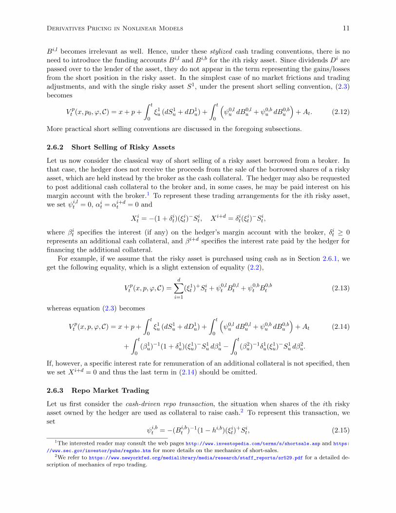
Bi,l becomes irrelevant as well. Hence, under these stylized cash trading conventions, there is noneed to introduce the funding accounts Bi,l and Bi,b for the ith risky asset. Since dividends Di arepassed over to the lender of the asset, they do not appear in the term representing the gains/lossesfrom the short position in the risky asset. In the simplest case of no market frictions and tradingadjustments, and with the single risky asset S1, under the present short selling convention, (2.3)becomes
V pt (x, p0, ϕ, C) = x+ p+
∫ t
0ξ1u (dS1
u + dD1u) +
∫ t
0
(ψ0,lu dB0,l
u + ψ0,bu dB0,b
u
)+At. (2.12)
More practical short selling conventions are discussed in the foregoing subsections.
2.6.2 Short Selling of Risky Assets
Let us now consider the classical way of short selling of a risky asset borrowed from a broker. Inthat case, the hedger does not receive the proceeds from the sale of the borrowed shares of a riskyasset, which are held instead by the broker as the cash collateral. The hedger may also be requestedto post additional cash collateral to the broker and, in some cases, he may be paid interest on hismargin account with the broker.1 To represent these trading arrangements for the ith risky asset,we set ψi,lt = 0, αit = αi+dt = 0 and
Xit = −(1 + δit)(ξ
it)−Sit , Xi+d = δit(ξ
it)−Sit ,
where βit specifies the interest (if any) on the hedger’s margin account with the broker, δit ≥ 0represents an additional cash collateral, and βi+d specifies the interest rate paid by the hedger forfinancing the additional collateral.
For example, if we assume that the risky asset is purchased using cash as in Section 2.6.1, weget the following equality, which is a slight extension of equality (2.2),
V pt (x, p, ϕ, C) =
d∑i=1
(ξ1t )+Sit + ψ0,lt B
0,lt + ψ0,b
t B0,bt (2.13)
whereas equation (2.3) becomes
V pt (x, p, ϕ, C) = x+ p+
∫ t
0ξ1u (dS1
u + dD1u) +
∫ t
0
(ψ0,lu dB0,l
u + ψ0,bu dB0,b
u
)+At (2.14)
+
∫ t
0(β1u)−1(1 + δ1u)(ξ1u)−S1
u dβ1u −
∫ t
0(β2u)−1δ1u(ξ1u)−S1
u dβ2u.
If, however, a specific interest rate for remuneration of an additional collateral is not specified, thenwe set Xi+d = 0 and thus the last term in (2.14) should be omitted.
2.6.3 Repo Market Trading
Let us first consider the cash-driven repo transaction, the situation when shares of the ith riskyasset owned by the hedger are used as collateral to raise cash.2 To represent this transaction, weset
ψi,bt = −(Bi,bt )−1(1− hi,b)(ξit)+Sit , (2.15)
1The interested reader may consult the web pages http://www.investopedia.com/terms/s/shortsale.asp and https:
//www.sec.gov/investor/pubs/regsho.htm for more details on the mechanics of short-sales.2We refer to https://www.newyorkfed.org/medialibrary/media/research/staff_reports/sr529.pdf for a detailed de-
scription of mechanics of repo trading.

12 T.R. Bielecki, I. Cialenco and M. Rutkowski
where Bi,b specifies the interest paid to the lender by the hedger who borrows cash and pledges therisky asset Si as collateral, and the constant hi,b represents the haircut for the ith asset pledged.
A synthetic short-selling of the risky asset Si using the repo market is obtained through thesecurity-driven repo transaction, that is, when shares of the risky asset are posted as collateral bythe borrower of cash and they are immediately sold by the hedger who lends the cash. Formally,this situation corresponds to the equality
ψi,lt = (Bi,lt )−1(1− hi,l)(ξit)−Sit (2.16)
where Bi,l specifies the interest amount paid to the hedger by the borrower of the cash amount(1− hi,l)(ξit)−Sit and hi,l is the corresponding haircut.
If only one risky asset is traded and transactions are exclusively in repo market, then we obtain
V pt (x, p, ϕ, C) = x+ p+
∫ t
0ξ1u (dS1
u + dD1u) +
∫ t
0
(ψ0,lu dB0,l
u + ψ0,bu dB0,b
u
)(2.17)
+
∫ t
0
((B1,l
u )−1(1− h1,l)(ξ1u)−S1u dB
1,lu − (B1,b
u )−1(1− h1,b)(ξ1u)+S1u dB
1,bu
)+At.
In practice, it is reasonable to assume that the long and short repo rates for a given riskyasset are identical, that is, Bi,l = Bi,b. In that case, we may and do set Bi := Bi,l = Bi,b andψit = (1− hi)(Bi
t)−1ξitS
it , so that equations (2.15) and (2.16) reduce to just one equation
(1− hi)ξitSit + ψitBit = 0. (2.18)
According to this interpretation of Bi, equality (2.18) means that trading in the ith risky asset isdone using the (symmetric) repo market and ξit shares of a risky asset are pledged as collateral attime t, meaning that the collateral rate equals 1. Under (2.18), equation (2.17) reduces to
V pt (x, p, ϕ, C) = x+ p+
∫ t
0ξ1u (dS1
u + dD1u) +
∫ t
0
(ψ0,lu dB0,l
u + ψ0,bu dB0,b
u
)(2.19)
−∫ t
0(B1
u)−1(1− h1)ξ1uS1u dB
1u +At.
2.7 Collateralization
We consider the situation when the hedger and the counterparty enter a contract and either receiveor pledge collateral with value denoted by C, which is assumed to be a semimartingale. Generallyspeaking, the process C represents the value of the margin account. We let
Ct = X1t +X2
t , (2.20)
where X1t := C+
t = Ct1Ct≥0, and X2t := −C−t = Ct1Ct<0. By convention, the amount C+
t is
the cash value of collateral received at time t by the hedger from the counterparty, whereas C−trepresents the cash value of collateral pledged by him and thus transferred to his counterparty.For simplicity of presentation and consistently with the prevailing market practice, it is postulatedthroughout that only cash collateral may be delivered or received (for other collateral conventions,see, e.g., [BR15]). According to ISDA Margin Survey 2014, about 75% of non-cleared OTC collateralagreements are settled in cash and about 15% in government securities. We also make the followingnatural assumption regarding the value of the margin account at the contract’s maturity date.
Assumption 2.6. The G-adapted collateral amount process C satisfies CT = 0.

Derivatives Pricing in Nonlinear Models 13
Typically this means that the collateral process C will have a jump at time T from CT− to 0.The postulated equality CT = 0 is simply a convenient way of ensuring that any collateral amountposted is returned in full to the pledger when the contract matures, provided that the default eventshave not occurred prior to or at maturity date T . As soon as the default events are also modeled,we will need to specify the closeout payoff (see Section 2.8.1).
Let us first make some comments from the hedger’s perspective regarding the crucial features ofthe margin account. The financial practice may require to hold the collateral amounts in segregatedmargin accounts, so that the hedger, when he is a collateral taker, cannot make use of the collateralamount for trading. Another collateral convention mostly encountered in practice is rehypothecation(around 90% of cash collateral of OTC contracts are rehypothecated), which refers to the situationwhere the hedger may use the collateral pledged by his counterparties as collateral for his contractswith other counterparties. Obviously, if the hedger is a collateral provider, then a particularconvention regarding segregation or rehypothecation is immaterial for the dynamics of the valueprocess of his portfolio. We refer the reader to [BR15] and [CBB14] for a detailed analysis of variousconventions on collateral agreements. Here we will examine some basic aspects of collateralization(sometimes also called margining) in our context.
In general, we have
$t = α1tC
+t − α2
tC−t −
∫ t
0(β1u)−1C+
u dβ1u +
∫ t
0(β2u)−1C−u dβ
2u, (2.21)
where the remuneration processes β1 and β2 determine the interest rates paid or received by thehedger on collateral amounts C+ and C−, respectively. The auxiliary processes α1 and α2 intro-duced in (2.21) are used to cover alternative conventions regarding rehypothecation and segregationof margin accounts. Note that we always set α2
t = 1 for all t ∈ [0, T ] when considering the portfolioof the hedger, since a particular convention regarding rehypothecation or segregation is manifestlyirrelevant for the pledger of collateral.
2.7.1 Rehypothecated Collateral
As it is customary in the existing literature, we assume that rehypothecation of cash collateralmeans that it can be used by the hedger for his trading purposes without any restrictions. To coverthis stylized version of a rehypothecated collateral for the hedger, it suffices to set α1
t = α2t = 1
for all t ∈ [0, T ], so that for the hedger we obtain α1tX
1t + α2
tX2t = Ct. Consequently, the cash
adjustment corresponding to the margin account equals
$t = $1t +$2
t =
2∑k=1
(Xk
0 +
∫ t
0βku dX
ku
). (2.22)
2.7.2 Segregated Collateral
Under segregation, the collateral received by the hedger is kept by the third party, so that it cannotbe used by the hedger for his trading activities. In that case, we set α1
t = 0 and α2t = 1 for all
t ∈ [0, T ] and thus α1tX
1t +α2
tX2t = −C−t . Hence the corresponding cash adjustment term $ equals
$t = $1t +$2
t = X20 −
∫ t
0X1u dβ
1u +
∫ t
0β2u dX
2u. (2.23)

14 T.R. Bielecki, I. Cialenco and M. Rutkowski
2.7.3 Initial and Variation Margins
In market practice, the total collateral amount is usually represented by two components, whichare termed the initial margin (also known as the independent amount) and the variation margin. Inthe context of self-financing trading strategies, this can be easily dealt with by introducing two (ormore) collateral processes for a given contract A. It is worth mentioning that each of the collateralprocesses specified in the clauses of a contract is usually subject to a different convention regardingsegregation and/or remuneration.
2.8 Counterparty Credit Risk
The counterparty credit risk in a financial contract arises from the possibility that at least one ofthe parties in the contract may default prior to or at the contract’s maturity, which may result infailure of this party to fulfil all their contractual obligations leading to financial loss suffered byeither one of the two parties in the contract. We will model defaultability of the two parties to thecontract in terms of their default times. We denote by τh and τ c the default times of the hedgerand his counterparty, respectively. We require that τh and τ c are non-negative random variablesdefined on (Ω,G,G,P). If τh > T holds a.s. (resp., τ c > T , a.s.) then the hedger (resp., thecounterparty) is considered to be default-free, at least with respect to the contract under study.Hence the counterparty risk is a relevant aspect of our model provided that P(τ ≤ T ) > 0, whereτ := τh ∧ τ c is the moment of the first default.
From now on, we postulate that the process A models all promised (or nominal) cash flows of thecontract, as seen from the perspective of the trading desk without taking into account the possibilityof defaults of trading parties. In other words, A represents cash flows that would be realized in casenone of the two parties defaulted prior to or at the contract’s maturity. We will sometimes refer toA as to the counterparty risk-free cash flows or counterparty clean cash flows and we will call thecontract with cash flows A the counterparty risk-free contract or the counterparty clean contract.The key concept in the context of counterparty risk is the counterparty risky contract.
2.8.1 Closeout Payoff
On the event τ <∞, we define the random variable Υ as
Υ = Qτ + ∆Aτ − Cτ , (2.24)
where Q is the Credit Support Annex (CSA) closeout valuation process of the contract A, ∆Aτ =Aτ − Aτ− is the jump of A at τ corresponding to a (possibly null) promised bullet dividend at τ ,and Cτ is the value of the collateral process C at time τ . In the financial interpretation, Υ+ is theamount the counterparty owes to the hedger at time τ , whereas Υ− is the amount the hedger owesto the counterparty at time τ . It accounts for the legal value Qτ of the contract, plus the bulletdividend ∆Aτ to be received/paid at time τ , less the collateral amount Cτ since it is already heldby the hedger (if Cτ > 0) or by the counterparty (if Cτ < 0). We refer the reader to [CBB14,Section 3.1.3] for more details regarding the financial interpretation of Υ.
One of the key financial aspects of the counterparty risky contract is the closeout payoff, whichoccurs if at least one of the parties defaults either before or at the maturity of the contract.It represents the cash flow exchanged between the two parties at first-party-default time. Thefollowing definition of the closeout payoff, as seen from the perspective of the hedger, is taken from[CBB14]. The random variables Rc and Rh, which take values in [0, 1], represent the recovery ratesof the counterparty and the hedger, respectively.

Derivatives Pricing in Nonlinear Models 15
Definition 2.7. The CSA closeout payoff K is defined as
K := Cτ + 1τc<τh(RcΥ+ −Υ−) + 1τh<τc(Υ
+ −RhΥ−) + 1τh=τc(RcΥ+ −RhΥ−). (2.25)
The counterparty risky cumulative cash flows process A] is given by
A]t = 1t<τAt + 1t≥τ(Aτ− + K), t ∈ [0, T ]. (2.26)
Let us make some comments on the form of the closeout payoff K. First, the term Cτ is due tothe fact that legal title to the collateral amount comes into force only at the time of the first default.The following three terms correspond to the CSA convention that, in principle, the nominal cashflow at the first default from the perspective of the hedger is given as Qτ + ∆Aτ . Let us consider,for instance, the event τc < τh. If Υ+ > 0, then we obtain
K = Cτ +Rc(Qτ + ∆Aτ − Cτ ) ≤ Qτ + ∆Aτ ,
where the equality holds whenever Rc = 1. If Υ− > 0, then we get
K = Cτ − (−Qτ −∆Aτ + Cτ ) = Qτ + ∆Aτ .
Finally, if Υ = 0, then K = Cτ = Qτ + ∆Aτ . Similar analysis can be done on the remaining twoevents in (2.25).
Remark 2.8. Of course, there is no counterparty credit risk present under the assumption thatP(τ > T ) = 1. Let us consider the case where P(τ > T ) < 1. We denote by pet the clean (that is,counterparty risk-free) ex-dividend price of the contract at time t. If we set Rc = Rh = 1, then weobtain
A]τ = Aτ +Qτ .
Hence the counterparty credit risk is still present, despite the postulate of the full recovery, unlessthe legal value Qτ perfectly matches the clean ex-dividend price peτ . Obviously, the counterpartycredit risk vanishes when Rc = Rh = 1 and Qτ = peτ , since in that case the so-called exposure atdefault (see [CBB14, Section 3.2.3]) is null.
2.8.2 Counterparty Credit Risk Decomposition
To effectively deal with the closeout payoff in our general framework, we now define the counterpartycredit risk (CCR) cash flows, which are sometimes called CCR exposures. Note that the eventsτ = τh = τh ≤ τ c and τ = τ c = τ c ≤ τh may overlap.
Definition 2.9. By the CCR processes, we mean the processes CL,CG and RP where the creditloss CL equals
CLt = −1t≥τ1τ=τc(1−Rc)Υ+,
the credit gain CG equals
CGt = 1t≥τ1τ=τh(1−Rh)Υ−,
and the replacement process is given by
CRt = 1t≥τ(Aτ −At +Qτ ).
The CCR cash flow is given by ACCR = CL+ CG+ CR.

16 T.R. Bielecki, I. Cialenco and M. Rutkowski
It is worth noting that the CCR cash flows depend on processes A,C and Q. The next propo-sition shows that we may interpret the counterparty risky contract as the clean contract A, whichis complemented by the collateral adjustment process X = (X1, X2) = (C+,−C−) and the CCRcash flow ACCR. In view of this result, the counterparty risky contract (A],X ) admits the followingformal decompositions (A],X ) = (A,X ) + (ACCR, 0) and (A],X ) = (A, 0) + (ACCR,X ).
Proposition 2.10. The equality A]t = At +ACCRt holds for all t ∈ [0, T ].
Proof. We first note that
K = Cτ + 1τc<τh(RcΥ+ −Υ−) + 1τh<τc(Υ
+ −RhΥ−) + 1τh=τc(RcΥ+ −RhΥ−)
= Cτ − 1τc≤τh(1−Rc)Υ+ + 1τh≤τc(1−Rh)Υ− + Υ
= Qτ + ∆Aτ − 1τc≤τh(1−Rc)Υ+ + 1τh≤τc(1−Rh)Υ−
where we used (2.24) in the last equality. Therefore, from (2.26) we obtain
A]t = 1t<τAt + 1t≥τ(Aτ− + K) = 1t<τAt + 1t≥τ(Aτ −∆Aτ + K)
= At∧τ + 1t≥τ(K−∆Aτ ) = At + (At∧τ −At) + 1t≥τ(K−∆Aτ )
= At + 1t≥τ(Aτ −At +Qτ − 1τc≤τh(1−Rc)Υ+ + 1τh≤τc(1−Rh)Υ−
),
which is the desired equality in view of Definition 2.9.
More generally, given two contracts, say (Ai,X i) for i = 1, 2, we are interested in pricingand hedging issues for a compound contract (A,X ) where A = f(A1, A2) in relation to pricingand hedging of its components (A1,X 1) and (A2,X 2). To be more specific, we wish to find outwhether individual no-arbitrage pricing for (A1,X 1) and (A2,X 2) leads to, at least approximate,fair valuation for the contract (A,X ). We need to stress that there may be a feedback effect involvedbetween the compound contract and its components. For instance, it follows from Proposition 2.10that the counterparty risky contract can be decomposed into the clean component (A1,X 1) =(A,X ) and the CCR component (A2,X 2) = (ACCR, 0). In bank’s practice, the exit price for acounterparty risky contract is the combination of the clean price of the contract and the price ofthe counterparty credit risk, which is referred to as the CCR price in what follows. The clean priceand the corresponding hedge are established by the trading desk, whereas the price and hedge forthe counterparty credit risk are dealt with by the dedicated CVA desk. To sum up, the typicalprocedure used in industry to derive the exit price of the contract (A],X ) is based on the followingadditive decomposition
price (A],X ) = price (A,X ) + price (ACCR, 0) = clean price + CCR price. (2.27)
It is unclear under which conditions this procedure results in an overall arbitrage-free valuationand hedging of the counterparty risky contract, in general, since the implicitly assumed additivityof pricing does not necessarily hold under market frictions.
In the existing literature, the counterpart of the above relationship is usually represented bythe equality
counterparty risky price = clean price− TVA
where TVA stands for the total valuation adjustment. This requires two comments. First, theTVA term accounts for several adjustments, and not only the counterparty credit risk, typicallyrepresented by the CVA and DVA. In particular, it may account for the funding valuation adjust-ment (FVA). In our approach, the funding adjustment results from the funding costs attributed to

Derivatives Pricing in Nonlinear Models 17
hedging the two components of (A],X ). Second, in our formula we have the sum, rather than thedifference, in the right-hand side of (2.27). This discrepancy is simply due to our definition of theadjustments CL, CG and CR, which are set to be negatives of their counterparts encountered inother papers.
2.9 Regulatory Capital
The case of the regulatory capital can be formally covered by adding the process Xk = −K, whereK is a non-negative stochastic process and by setting αkt = 1 for all t ∈ [0, T ]. If the regulatorycapital is remunerated, then we also need to specify the corresponding remuneration process βk. Ofcourse, an important issue of explicit specifications of these processes will arise when the generaltheory is implemented. A practical approach to the capital valuation adjustment associated withthe regulatory capital was developed in a recent work by Albanese et al. [ACC16].
3 Arbitrage-Free Trading Models
The analysis of the self-financing property of a trading strategy should be complemented by thestudy of some kind of a no-arbitrage property for the adopted market model. Due to the nonlinearityof a market model with differential funding rates, the concept of no-arbitrage is nontrivial, evenwhen no trading adjustments are present. We will argue that it can be effectively dealt with using areasonably general definition of an arbitrage opportunity associated with trading. Let us stress thatwe only consider here a nonlinear extension of the classical concept of an arbitrage opportunity (asopposed to other related concepts, such as: NFLVR, NUPBR, etc.).
3.1 No-arbitrage Pricing Principles
Let us first describe very briefly the commonly adopted pricing paradigm for financial derivatives.In essence, a general approach to no-arbitrage pricing hinges on the following steps:
Step (L.1). One first checks whether a market model with predetermined trading rules and primarytraded assets is arbitrage-free, where the definition of an arbitrage opportunity is a mathematicalformalization of the real-world concept of a risk-free profitable trading opportunity.
Step (L.2). Given a financial derivative for which the price is yet unspecified, one proposes aprice (not necessarily unique) and checks whether the extended model (that is, the model wherethe financial derivative is postulated to be an additional traded asset) is also arbitrage-free in thesense made precise in Step (L.1).
The valuation procedure outlined above can be referred to as the no-arbitrage pricing paradigm.In any linear market model (see the comments after Definition 2.3), the unique price given by repli-cation (or the range of no-arbitrage prices obtained using the concept of superhedging strategies inthe case of an incomplete market) is consistent with the no-arbitrage pricing paradigm (L.1)–(L.2),although to establish this property in a continuous-time framework, one needs also to introduce theconcept of admissibility of a trading strategy. This is feasible since the strict comparison propertyof linear BSDEs can be employed to show that replication (or superhedging) will indeed yield pricesfor derivatives that are consistent with the no-arbitrage pricing paradigm. Alternatively, the fun-damental theorem of asset pricing (FTAP) can be used to show that the discounted prices definedthrough admissible trading strategies are local martingales (in fact, supermartingales) under anequivalent local martingale measure. The latter property is a well known fundamental feature ofstochastic integration, so it covers all linear market models.

18 T.R. Bielecki, I. Cialenco and M. Rutkowski
Let us now comment on the existing approaches to nonlinear pricing of derivatives. The mostcommon approach to the pricing problem in a nonlinear framework seems to hinge, at least implic-itly, on the following steps in which it is usually assumed that the hedger’s initial endowment isnull. In fact, Step (N.1) was explicitly addressed only in some works, whereas most papers in theexisting literature were concerned with finding a replicating strategy mentioned in Step (N.2). Also,to the best of our knowledge, the important issue outlined in Step (N.3) was up to now completelyignored.
Step (N.1). The strict comparison argument for the BSDE associated with the wealth dynamicsis used to show that it is not possible to construct an admissible trading strategy with the nullinitial wealth and the terminal wealth, which is non-negative almost surely and strictly positivewith a positive probability.
Step (N.2). The price for a European contingent claim is defined using either the cost of replicationor the minimal cost of superhedging. A suitable version of the strict comparison property for thewealth dynamics can be used to show that in some market models (referred to as regular modelsin this work) the two pricing approaches yield the same value for any European claim that can bereplicated.
Step (N.3). It remains to check if the prices given by the cost of replication (or selected to bebelow the upper bound given by the minimal cost of superhedging) comply with some form of theno-arbitrage principle.
The problem whether the extended nonlinear market model is still arbitrage-free in some senseis much harder to tackle than it was the case for the linear framework, since trading in derivativesmay essentially change the properties of the market. However, in the case of a regular model, thisstep is relatively easy to handle due to the postulated regularity conditions (see, in particular,Definition 4.6 and Proposition 4.8).
3.2 Discounted Wealth and Admissible Strategies
To deal with the issue of no-arbitrage, we need to introduce the discounted wealth process andproperly define the concept of admissibility of trading strategies. Let us denote
Bt(x) := 1x≥0B0,lt + 1x<0B
0,bt . (3.1)
Note that if B0,l = B0,b, then B(x) = B0 = B. Furthermore, if x = 0, then xB0,bT = xB0,l
T = 0 andthus the choice of either B0,l or B0,b in the right-hand side of (3.1) is immaterial. It is natural to
postulate that the initial endowment x ≥ 0 (resp. x < 0) has the future value xB0,lt (resp. xB0,b
t )at time t ∈ [0, T ] when invested in the cash account B0,l (resp. B0,b). We thus henceforth workunder the following assumption.
Assumption 3.1. We postulate that:
(i) for any initial endowment x ∈ R of the hedger, the null contract N = (0, 0) belongs to C ,
(ii) for any x ∈ R, the trading strategy (x, 0, ϕ,N ) where ϕ has all components null except foreither ψ0,l (if x ≥ 0) or ψ0,b (if x < 0) belongs to Φ0,x(C ) and V p
t (x, 0, ϕ,N ) = Vt(x, 0, ϕ,N ) =xBt(x) for all t ∈ [0, T ].
Assumption 3.1 may look redundant at the first glance, but it is nevertheless needed and usefulin derivation of basic properties of fair prices. Condition (i) is a rather obvious requirement. Notethat condition (ii) cannot be deduced directly from the self-financing condition, since it hinges onthe additional postulate that there are no trading adjustments (such as: taxes, transactions costs,

Derivatives Pricing in Nonlinear Models 19
margin account, etc.) when the initial endowment is invested in the cash account. Formally, itstates that the null contract N = (0, 0) can be entered into by the hedger and it be will used toshow that the null contract has zero fair price at any date t ∈ [0, T ]. Also, the trading strategyintroduced in condition (ii) will serve as a natural benchmark for assessment of profits or lossesincurred by the hedger.
We also follow the standard approach of introducing the concept of admissibility for the dis-counted wealth. Towards this end, for any fixed t ∈ [0, T ) we consider a hedger who starts tradingat time t with the initial endowment xt and who uses a self-financing trading strategy (xt, pt, ϕ
t, Ct),where the price pt ∈ Gt at which the contract Ct is traded at time t is arbitrary. We also considerthe discounting process Bt(xt) on [t, T ], which is given by
Btu(xt) := 1xt≥0B0,lu (B0,l
t )−1 + 1xt<0B0,bu (B0,b
t )−1, (3.2)
so that, in particular, Btt(xt) = xt. Then the wealth process discounted back to time t satisfies
Vu(xt, pt, ϕt, Ct) := (Btu(xt))
−1Vu(xt, pt, ϕt, Ct), u ∈ [t, T ], (3.3)
and we have the following natural concept of admissibility of a trading strategy on [t, T ].
Definition 3.2. Let t ∈ [0, T ). We say that a trading strategy (xt, pt, ϕt, Ct) ∈ Φt,xt(C ) is admis-
sible if the discounted wealth Vu(xt, pt, ϕt, Ct) is bounded from below by a constant. We denote by
Ψt,xt(pt, Ct) the class of admissible strategies corresponding to (xt, pt, ϕt, Ct), and we let
Ψt,xt(C ) := ∪C∈C ∪pt∈Gt Ψt,xt(pt, Ct)
to denote the class of all admissible trading strategies on [t, T ] relative to the class C of contractsfor the hedger with the initial endowment xt at time t. In particular, Ψ0,x(C ) represents the classof all trading strategies admissible at time t = 0 for the hedger with the initial endowment x.
3.3 No-arbitrage with Respect to the Null Contract
A minimal no-arbitrage requirement for an underlying market model is that it should be arbitrage-free with respect to the null contract. Note that, consistently with Assumption 3.1 and the conceptof replication (for the general formulation of replication of a non-null contract, see Definition 4.4),it is implicitly assumed in Definition 3.3 that the price at which the null contract is traded at timezero equals zero. Needless to say, this is a rather obvious postulate in any trading model.
Definition 3.3. Consider an underlying market model M = (S,D,B,C ,Ψ0,x(C )). An arbitrageopportunity with respect to the null contract (or a primary arbitrage opportunity) for the hedgerwith an initial endowment x is a strategy (x, 0, ϕ,N ) ∈ Ψ0,x(0,N ) such that
P(VT (x, 0, ϕ,N ) ≥ x) = 1, P(VT (x, 0, ϕ,N ) > x) > 0. (3.4)
If no primary arbitrage opportunity exists in the market modelM then we say thatM is arbitrage-free with respect to the null contract for the hedger with an initial endowment x.
For any linear market model, Definition 3.3 reduces to the classical definition of an arbitrageopportunity. It is well known that the no-arbitrage property introduced in this definition is asufficiently strong tool for the development of no-arbitrage pricing for financial derivatives in thelinear framework. This does not mean, however, that Definition 3.3 is sufficiently strong to allowus to develop nonlinear no-arbitrage pricing theory, which would enjoy the properties, which aredesirable from either mathematical or financial perspective. On the one hand, a natural definition

20 T.R. Bielecki, I. Cialenco and M. Rutkowski
of a hedger’s fair value (see Definition 4.1) is consistent with the concept of no-arbitrage withrespect to the null contract and thus it seems to be theoretically sound. On the other hand, as weargue below, Definition 3.3 is manifestly not sufficient to ensure an efficient pricing and hedgingapproach in a general nonlinear market.
First, it may occur that the replication cost of a contract does not satisfy the definition of a fairprice, since selling of a contract at its replication cost may generate an arbitrage opportunity for thehedger. Explicit examples of market models, which are arbitrage-free in the sense of Definition 3.3,but suffer from this deficiency, are given in Section 7.1.
Second, and more importantly, not well established method of finding a fair price in a generalnonlinear market satisfying Definition 3.3 is available. We contend that the drawback of the defini-tion of an arbitrage-free model with respect to the null contract is that it does not make an explicitreference to a class C of contracts under study. Indeed, it hinges on the specification of the classΨ0,x(0,N ) of trading strategies, but it does not take into account the larger class Ψ0,x(C ). Toamend this drawback of Definition 3.3, it was proposed in [BR15] to consider the concept of theno-arbitrage for the trading desk with respect to a predetermined family C of contracts.
3.4 No-arbitrage for the Trading Desk
Following [BR15], we will now examine a stronger no-arbitrage property of a model, which is directlyrelated to a predetermined family C of contracts. The goal to impose a more stringent no-arbitragecondition, which not only accounts for the nonlinearity of the market, but also explicitly refers toa family of contracts under consideration. Regrettably, the class of models that are arbitrage-freein the sense of Definition 3.7 could still be too encompassing, and thus it is unclear whether thepricing irregularities mentioned in the preceding section will be eliminated (for an example, seeSection 7.2).
For simplicity of notation, we consider here the case of t = 0, but all definitions can be extendedto the case of any date t. The symbols X = X (A) and Y = Y(−A) are used to emphasize that thereis no reason to expect that the trading adjustments will satisfy the equality X (−A) = −X (A), ingeneral. Therefore, we denote by Y = (Y 1, . . . , Y n;α1(Y), . . . , αn(Y);β1(Y), . . . , βn(Y)) the tradingadjustments associated with the cumulative cash flows process −A. In order to avoid confusion, wewill use the full notation for the wealth process, for instance, V (x, p, ϕ, C) = V (x, p, ϕ,A,X ), etc.
Definition 3.4. For a contract C = (A,X ) and an initial endowment x, the combined wealth isdefined as
V com(x1, x2, ϕ, ϕ, A,X ,Y) := V (x1, 0, ϕ,A,X ) + V (x2, 0, ϕ,−A,Y), (3.5)
where x1, x2 are any real numbers such that x = x1 + x2, ϕ ∈ Ψ0,x1(0, A,X ), ϕ ∈ Ψ0,x2(0,−A,Y).In particular, V com
0 (x1, x2, ϕ, ϕ, A,X ,Y) = x1 + x2 = x.
The rationale for the term combined wealth comes from the financial interpretation of the processgiven by the right-hand side in (3.5). We argue that it represents the aggregated wealth of twotraders, which are members of the same trading desk, who are supposed to act as follows:
• The first trader takes the long position in a contract (A,X ), whereas the second one takesthe short position in the same contract, which is thus formally represented by (−A,Y). Sincewe assume that the long and short positions have exactly opposite prices, the correspondingcash flows p and −p coming to the trading desk (and not to individual traders) offset eachother and thus the initial endowment x of the trading desk remains unchanged.

Derivatives Pricing in Nonlinear Models 21
• In addition, it is assumed that after the cash flows p and −p have been netted so they areno longer present, the initial endowment x is split into arbitrary amounts x1 and x2 meaningthat x = x1 +x2. Then each trader is allocated the respective amount x1 and x2 as an initialendowment and each of them hedges his position. It is now clear that the level of the initialprice p at which the contract is traded at time zero is immaterial for both hedging strategiesand the combined wealth of the two traders is given by the right-hand side in (3.5).
Alternatively, the combined wealth may be used to describe the situation where a single tradertakes long and short positions with two external counterparties and hedges them independentlyusing his initial endowment x split into x1 and x2. Of course, in that case it is even more clearthat the initial price p has no impact on his trading strategies.
Remark 3.5. One can also observe that the following equality is manifestly satisfied for any realnumber p
V (x1, 0, ϕ,A,X ) + V (x2, 0, ϕ,−A,Y) = V (x1, p, ϕ,A,X ) + V (x2,−p, ϕ,−A,Y),
where x1 = x1 − p and x2 = x2 + p is another decomposition of x such that x = x1 + x2. However,equation (3.5) much better reflects the actual trading arrangements and it has a clear advantagethat an unknown number p does not appear in the formula for the combined wealth. It thusemphasizes the crucial feature that the combined wealth is independent of p. In fact, one canremark that the issue whether the trading desk has been informed about the actual level of theprice p does not matter at all.
Definition 3.6. A pair (x1, ϕ;x2, ϕ) of trading strategies introduced in Definition 3.4 is admissiblefor the trading desk if the discounted combined wealth process
V com(x1, x2, ϕ, ϕ, A,X ,Y) := (B(x))−1V com(x1, x2, ϕ, ϕ, A,X ,Y) (3.6)
is bounded from below by a constant. The class of such strategies is denoted by Ψ0,x1,x2(A,X ,Y).
We are in a position to formalize the concept of an arbitrage-free model for the trading deskwith respect to a particular family of contracts.
Definition 3.7. We say that a pair (x1, ϕ;x2, ϕ) ∈ Ψ0,x1,x2(A,X ,Y) is an arbitrage opportunityfor the trading desk with respect to a contract (A,X ) if the following conditions are satisfied
P(V comT (x1, x2, ϕ, ϕ, A,X ,Y) ≥ x) = 1, P(V com
T (x1, x2, ϕ, ϕ, A,X ,Y) > x) > 0.
We say that the market model M = (S,D,B,C ,Ψ0,x(C )) is arbitrage-free for the trading desk ifno arbitrage opportunity exists for the trading desk with respect to any contract C from C .
Our main purpose in Sections 3.3 and 3.4 was to provide some simple criteria that would allowone to eliminate models in which some particular form of arbitrage appears. Definition 3.3 andDefinition 3.7 provide such criteria for accepting or rejecting any tentative nonlinear market model.It is easy to see that a model which is rejected according to Definition 3.7 is also rejected whenDefinition 3.3 is applied. We do not claim, however, that these tests are sufficient to discriminatebetween acceptable and non-acceptable nonlinear models for pricing of derivatives. Indeed, inDefinition 4.6 we formulate additional conditions that should be satisfied by a viable market model.
22 T.R. Bielecki, I. Cialenco and M. Rutkowski
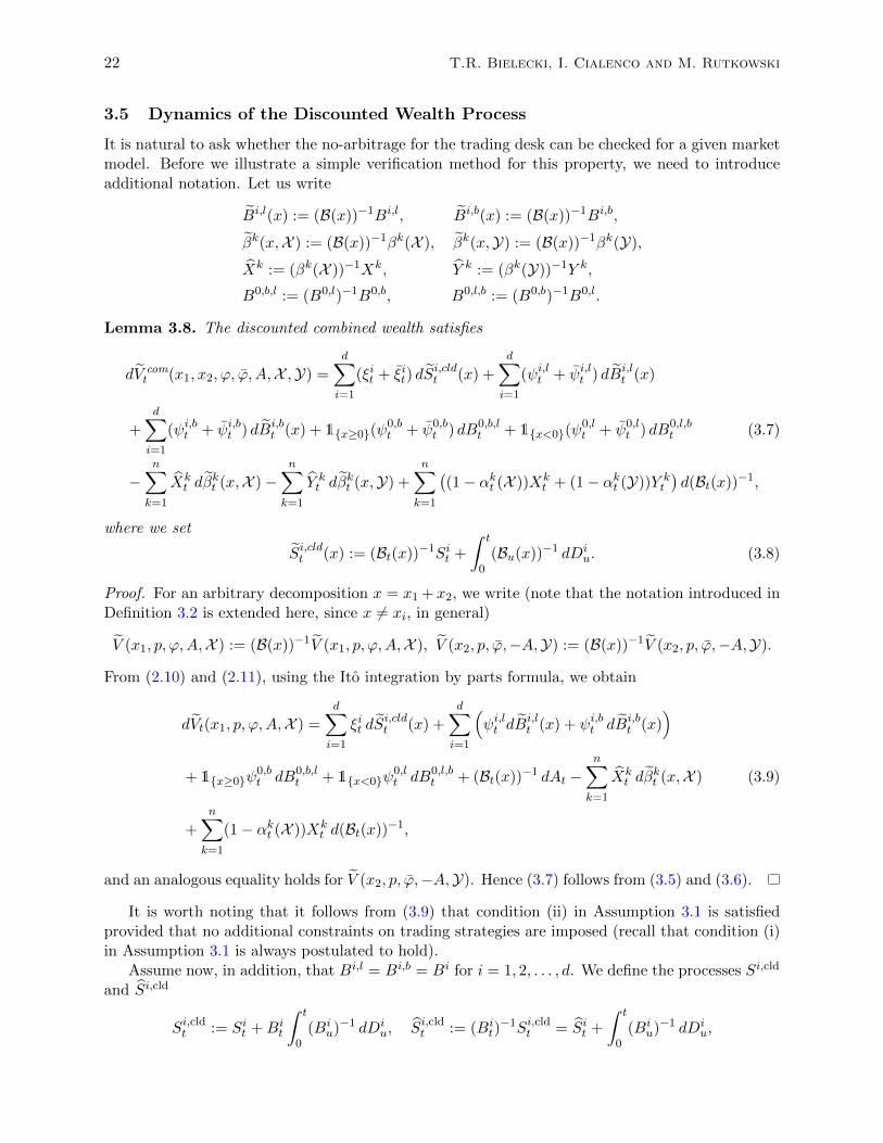
3.5 Dynamics of the Discounted Wealth Process
It is natural to ask whether the no-arbitrage for the trading desk can be checked for a given marketmodel. Before we illustrate a simple verification method for this property, we need to introduceadditional notation. Let us write
Bi,l(x) := (B(x))−1Bi,l, Bi,b(x) := (B(x))−1Bi,b,
βk(x,X ) := (B(x))−1βk(X ), βk(x,Y) := (B(x))−1βk(Y),
Xk := (βk(X ))−1Xk, Y k := (βk(Y))−1Y k,
B0,b,l := (B0,l)−1B0,b, B0,l,b := (B0,b)−1B0,l.
Lemma 3.8. The discounted combined wealth satisfies
dV comt (x1, x2, ϕ, ϕ, A,X ,Y) =
d∑i=1
(ξit + ξit) dSi,cldt (x) +
d∑i=1
(ψi,lt + ψi,lt ) dBi,lt (x)
+d∑i=1
(ψi,bt + ψi,bt ) dBi,bt (x) + 1x≥0(ψ
0,bt + ψ0,b
t ) dB0,b,lt + 1x<0(ψ
0,lt + ψ0,l
t ) dB0,l,bt (3.7)
−n∑k=1
Xkt dβ
kt (x,X )−
n∑k=1
Y kt dβ
kt (x,Y) +
n∑k=1
((1− αkt (X ))Xk
t + (1− αkt (Y))Y kt
)d(Bt(x))−1,
where we set
Si,cldt (x) := (Bt(x))−1Sit +
∫ t
0(Bu(x))−1 dDi
u. (3.8)
Proof. For an arbitrary decomposition x = x1 + x2, we write (note that the notation introduced inDefinition 3.2 is extended here, since x 6= xi, in general)
V (x1, p, ϕ,A,X ) := (B(x))−1V (x1, p, ϕ,A,X ), V (x2, p, ϕ,−A,Y) := (B(x))−1V (x2, p, ϕ,−A,Y).
From (2.10) and (2.11), using the Ito integration by parts formula, we obtain
dVt(x1, p, ϕ,A,X ) =
d∑i=1
ξit dSi,cldt (x) +
d∑i=1
(ψi,lt dB
i,lt (x) + ψi,bt dBi,b
t (x))
+ 1x≥0ψ0,bt dB0,b,l
t + 1x<0ψ0,lt dB0,l,b
t + (Bt(x))−1 dAt −n∑k=1
Xkt dβ
kt (x,X ) (3.9)
+n∑k=1
(1− αkt (X ))Xkt d(Bt(x))−1,
and an analogous equality holds for V (x2, p, ϕ,−A,Y). Hence (3.7) follows from (3.5) and (3.6).
It is worth noting that it follows from (3.9) that condition (ii) in Assumption 3.1 is satisfiedprovided that no additional constraints on trading strategies are imposed (recall that condition (i)in Assumption 3.1 is always postulated to hold).
Assume now, in addition, that Bi,l = Bi,b = Bi for i = 1, 2, . . . , d. We define the processes Si,cld
and Si,cld
Si,cldt := Sit +Bit
∫ t
0(Bi
u)−1 dDiu, Si,cldt := (Bi
t)−1Si,cldt = Sit +
∫ t
0(Bi
u)−1 dDiu,

Derivatives Pricing in Nonlinear Models 23
where in turn Si := (Bi)−1Si. It is easy to check that
dSi,cldt (x) = Bit(x) dSi,cldt + Sit dB
it(x), (3.10)
where Bi(x) := (B(x))−1Bi and thus (3.7) becomes
dV comt (x1, x2, ϕ, ϕ, A,X ,Y) =
d∑i=1
(ξit + ξit)Bit(x) dSi,cldt +
d∑i=1
((ξit + ξit)S
it + (ψit + ψit)
)dBi
t(x)
+ 1x≥0(ψ0,bt + ψ0,b
t ) dB0,b,lt + 1x<0(ψ
0,lt + ψ0,l
t ) dB0,l,bt −
n∑k=1
Xkt dβ
kt (x,X ) (3.11)
−n∑k=1
Y kt dβ
kt (x,Y) +
n∑k=1
((1− αkt (X ))Xk
t + (1− αkt (Y))Y kt
)d(Bt(x))−1.
3.6 Sufficient Conditions for the Trading Desk No-Arbitrage
The following result gives a sufficient condition for a market model to be arbitrage-free for thetrading desk. The proof of Proposition 3.9 is straightforward and thus it is omitted.
Proposition 3.9. Assume that there exists a probability measure Q, equivalent to P on (Ω,GT ), andsuch that for any decomposition x = x1 + x2 and any admissible combination of trading strategies(x1, ϕ,A,X ) and (x2, ϕ,−A,Y) for any contract (A,X ) belonging to C the discounted combinedwealth V com(x1, x2, ϕ, ϕ, A,X ,Y) is a supermartingale under Q. Then the market model M =(S,D,B,C ,Ψ0,x(C )) is arbitrage-free for the trading desk.
Although Proposition 3.9 is fairly abstract, the sufficient condition stated there can readily beverified as soon as a specific market model is adopted (see, for instance, [BR15, NR15, NR16a,NR16c]). To support this claim, we will examine a market model with idiosyncratic funding ofrisky assets and rehypothecated cash collateral.
Example 3.10. We consider the special case where B0,l = B0,b = B = B(x) and Bi,l = Bi,b = Bi
for all i = 1, 2, . . . , d. Under the assumption of no additional constraints on trading strategies,(3.11) yields (for a special case of this formula, see Corollary 2.1 in [BR15])
dV comt (x1, x2, ϕ, ϕ, A,X ,Y) =
d∑i=1
(ξit + ξit)Bit(x) dSi,cldt +
d∑i=1
(ξitSit + ψitB
it)(B
it)−1 dBi
t(x)
+d∑i=1
(ξitSit + ψitB
it)(B
it)−1 dBi
t(x)−n∑k=1
Xkt dβ
kt (x,X )−
n∑k=1
Y kt dβ
kt (x,Y)
+n∑k=1
((1− αkt (X ))Xk
t + (1− αkt (Y))Y kt
)dB−1t .
We postulate that the cash collateral is rehypothecated, so that n = 2 in Section 2.4. Thenα1t = α2
t = α1t (Y) = α2
t (Y) = 1 and X1t + Y 1
t = X2t + Y 2
t = 0 for all t ∈ [0, T ]. Let us assume, inaddition, that ξitS
it + ψitB
it = ξitS
it + ψitB
it = 0 for all i and t ∈ [0, T ], meaning that the ith risky
asset is fully funded from the repo account Bi (see Section 2.6.3). More generally, it suffices toassume that the following equalities are satisfied for all t ∈ [0, T ]
d∑i=1
∫ t
0(ξiuS
iu + ψiuB
iu)(Bi
u)−1 dBiu(x) =
d∑i=1
∫ t
0(ξiuS
iu + ψiuB
iu)(Bi
u)−1 dBiu(x) = 0. (3.12)
24 T.R. Bielecki, I. Cialenco and M. Rutkowski
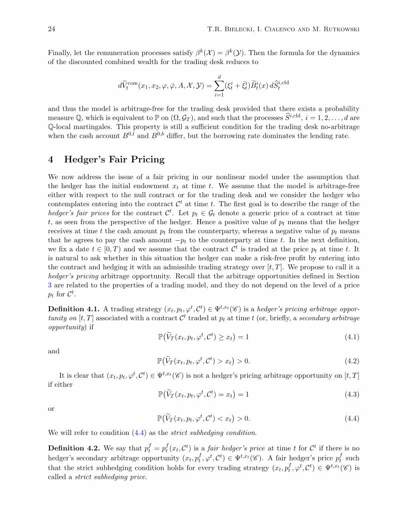
Finally, let the remuneration processes satisfy βk(X ) = βk(Y). Then the formula for the dynamicsof the discounted combined wealth for the trading desk reduces to
dV comt (x1, x2, ϕ, ϕ, A,X ,Y) =
d∑i=1
(ξit + ξit)Bit(x) dSi,cldt
and thus the model is arbitrage-free for the trading desk provided that there exists a probabilitymeasure Q, which is equivalent to P on (Ω,GT ), and such that the processes Si,cld, i = 1, 2, . . . , d areQ-local martingales. This property is still a sufficient condition for the trading desk no-arbitragewhen the cash account B0,l and B0,b differ, but the borrowing rate dominates the lending rate.
4 Hedger’s Fair Pricing
We now address the issue of a fair pricing in our nonlinear model under the assumption thatthe hedger has the initial endowment xt at time t. We assume that the model is arbitrage-freeeither with respect to the null contract or for the trading desk and we consider the hedger whocontemplates entering into the contract Ct at time t. The first goal is to describe the range of thehedger’s fair prices for the contract Ct. Let pt ∈ Gt denote a generic price of a contract at timet, as seen from the perspective of the hedger. Hence a positive value of pt means that the hedgerreceives at time t the cash amount pt from the counterparty, whereas a negative value of pt meansthat he agrees to pay the cash amount −pt to the counterparty at time t. In the next definition,we fix a date t ∈ [0, T ) and we assume that the contract Ct is traded at the price pt at time t. Itis natural to ask whether in this situation the hedger can make a risk-free profit by entering intothe contract and hedging it with an admissible trading strategy over [t, T ]. We propose to call it ahedger’s pricing arbitrage opportunity. Recall that the arbitrage opportunities defined in Section3 are related to the properties of a trading model, and they do not depend on the level of a pricept for Ct.
Definition 4.1. A trading strategy (xt, pt, ϕt, Ct) ∈ Ψt,xt(C ) is a hedger’s pricing arbitrage oppor-
tunity on [t, T ] associated with a contract Ct traded at pt at time t (or, briefly, a secondary arbitrageopportunity) if
P(VT (xt, pt, ϕ
t, Ct) ≥ xt)
= 1 (4.1)
and
P(VT (xt, pt, ϕ
t, Ct) > xt)> 0. (4.2)
It is clear that (xt, pt, ϕt, Ct) ∈ Ψt,xt(C ) is not a hedger’s pricing arbitrage opportunity on [t, T ]
if either
P(VT (xt, pt, ϕ
t, Ct) = xt)
= 1 (4.3)
or
P(VT (xt, pt, ϕ
t, Ct) < xt)> 0. (4.4)
We will refer to condition (4.4) as the strict subhedging condition.
Definition 4.2. We say that pft = pft (xt, Ct) is a fair hedger’s price at time t for Ct if there is no
hedger’s secondary arbitrage opportunity (xt, pft , ϕ
t, Ct) ∈ Ψt,xt(C ). A fair hedger’s price pft such
that the strict subhedging condition holds for every trading strategy (xt, pft , ϕ
t, Ct) ∈ Ψt,xt(C ) iscalled a strict subhedging price.

Derivatives Pricing in Nonlinear Models 25
It is clear from Definitions 4.2 and 4.1 that if pft is a fair price, then any trading strategiy(xt, pt, ϕ
t, Ct) ∈ Ψt,xt(C ) necessarily satisfies either condition (4.3) or condition (4.4). Obviously,a fair hedger’s price depends both on the given endowment xt and the contract Ct and thus thenotation pft (xt, Ct) is appropriate, but it will be frequently simplified to pft when no danger of
confusion may arise. It is important to note that if pft is a fair hedger’s price (resp. a strict
subhedging price) at time t for Ct, then any pt ≤ pft is also a fair hedger’s price (resp. a strict
subhedging price) at time t for that contract, provided that the amount pft −pt ≥ 0 can be investedin B0,l with no trading adjustments. Recall that the latter property has been already postulatedin our framework and thus it is not restrictive.
A fair price prevents the hedger from making sure profit with a positive probability and withno risk of losing money. In contrast, it does not prevent the hedger from losing money, in general.It is thus natural to search for the highest possible value of a fair price. This idea motivates thefollowing definition of the upper bound for the hedger’s fair prices
pft(xt, Ct) := ess sup
pft ∈ Gt | p
ft is a fair hedger’s price for Ct
. (4.5)
We find it useful to study also the upper bound for the strict subhedging prices, which is given by
pt(xt, Ct) := ess sup
pft ∈ Gt | p
ft is a strict subhedging price for Ct
. (4.6)
Definition 4.3. A trading strategy (xt, pst , ϕ
t, Ct) ∈ Ψt,xt(C ) is said to be a superhedging strategy fora contract Ct if (4.1) holds, whereas a strict superhedging means that (4.1) and (4.2) are satisfied. Inthe former (resp. latter) case, pst = pst (xt, Ct) is called a superhedging cost (resp. strict superhedgingcost) at time t for Ct.
If a superhedging (resp. strict superhedging) strategy exists when Ct is entered into at the pricepst , then a superhedging (resp. strict superhedging) strategy exists as well for any pt satisfyingpt ≥ pst . The lower bound for superhedging costs is given by
pst (xt, Ct) := ess infpst ∈ Gt | pst is a superhedging cost for Ct
(4.7)
and the lower bound for strict superhedging costs equals
pt(xt, Ct) := ess infpst ∈ Gt | pst is a strict superhedging cost for Ct
. (4.8)
For the basic relationships between the quantities introduced above when t = 0, see Lemma 4.5(analogous relationships hold in fact for any t > 0 as well, but they are not reported here).
In any linear (either complete or incomplete) market model, the quantities pt
and pt do notdepend on the hedger’s endowment. Moreover, the equality p
t= pt can be established in some
arbitrage-free incomplete models for all square-integrable European claims (see El Karoui andQuenez [EKQ95]). It was shown in [EKQ95] that the common value is not a fair hedger’s price fora European claim, unless it can be replicated. Of course, in the latter case we have that p
t= pt = pt
where pt denotes the unique cost of replication.Obviously, this does not mean that such desirable properties of p
t(xt, Ct), pt(xt, Ct) and the cost
of replication (see Definition 4.4) will still be valid when the assumption of a model’s linearity isrelaxed, even when a nonlinear model is assumed to be arbitrage-free either with respect to thenull contract or for the trading desk. Furthermore, Definition 4.2 is too broad, in the sense that itis not constructive and thus it does not offer any guidance how to implement fair pricing, let alonehow to derive the dynamics of fair prices for a given contract. These important shortcomings areaddressed and overcome in Section 4.2 where the notion of a regular market is introduced.
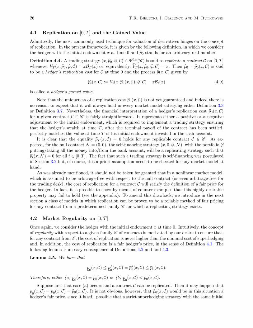
26 T.R. Bielecki, I. Cialenco and M. Rutkowski
4.1 Replication on [0, T ] and the Gained Value
Admittedly, the most commonly used technique for valuation of derivatives hinges on the conceptof replication. In the present framework, it is given by the following definition, in which we considerthe hedger with the initial endowment x at time 0 and p0 stands for an arbitrary real number.
Definition 4.4. A trading strategy (x, p0, ϕ, C) ∈ Ψ0,x(C ) is said to replicate a contract C on [0, T ]whenever VT (x, p0, ϕ, C) = xBT (x) or, equivalently, VT (x, p0, ϕ, C) = x. Then p0 = p0(x, C) is saidto be a hedger’s replication cost for C at time 0 and the process p(x, C) given by
pt(x, C) := Vt(x, p0(x, C), ϕ, C)− xBt(x) (4.9)
is called a hedger’s gained value.
Note that the uniqueness of a replication cost p0(x, C) is not yet guaranteed and indeed there isno reason to expect that it will always hold in every market model satisfying either Definition 3.3or Definition 3.7. Nevertheless, the financial interpretation of a hedger’s replication cost p0(x, C)for a given contract C ∈ C is fairly straightforward. It represents either a positive or a negativeadjustment to the initial endowment, which is required to implement a trading strategy ensuringthat the hedger’s wealth at time T , after the terminal payoff of the contract has been settled,perfectly matches the value at time T of his initial endowment invested in the cash account.
It is clear that the equality pT (x, C) = 0 holds for any replicable contract C ∈ C . As ex-pected, for the null contract N = (0, 0), the self-financing strategy (x, 0, ϕ,N ), with the portfolio ϕputting/taking all the money into/from the bank account, will be a replicating strategy such thatpt(x,N ) = 0 for all t ∈ [0, T ]. The fact that such a trading strategy is self-financing was postulatedin Section 3.2 but, of course, this a priori assumption needs to be checked for any market model athand.
As was already mentioned, it should not be taken for granted that in a nonlinear market model,which is assumed to be arbitrage-free with respect to the null contract (or even arbitrage-free forthe trading desk), the cost of replication for a contract C will satisfy the definition of a fair price forthe hedger. In fact, it is possible to show by means of counter-examples that this highly desirableproperty may fail to hold (see the appendix). To amend this drawback, we introduce in the nextsection a class of models in which replication can be proven to be a reliable method of fair pricingfor any contract from a predetermined family C for which a replicating strategy exists.
4.2 Market Regularity on [0, T ]
Once again, we consider the hedger with the initial endowment x at time 0. Intuitively, the conceptof regularity with respect to a given family C of contracts is motivated by our desire to ensure that,for any contract from C , the cost of replication is never higher than the minimal cost of superhedgingand, in addition, the cost of replication is a fair hedger’s price, in the sense of Definition 4.1. Thefollowing lemma is an easy consequence of Definitions 4.2 and and 4.3.
Lemma 4.5. We have that
p0(x, C) ≤ pf
0(x, C) = ps0(x, C) ≤ p0(x, C).
Therefore, either (a) p0(x, C) = p0(x, C) or (b) p
0(x, C) < p0(x, C).
Suppose first that case (a) occurs and a contract C can be replicated. Then it may happen thatp0(x, C) = p0(x, C) = p0(x, C). It is not obvious, however, that p0(x, C) would be in this situation a
hedger’s fair price, since it is still possible that a strict superhedging strategy with the same initial
Derivatives Pricing in Nonlinear Models 27
cost might exist. Furthermore, it may also happen that p0(x, C) < p0(x, C) meaning that a strictsuperhedging is less expensive than replication.
Suppose now that case (a) occurs but a contract C cannot be replicated. Then it is not clearwhether p0 := pf
0(x, C) = ps0(x, C) is a fair price, although we have that
p0(x, C) = pf
0(x, C) = ps0(x, C) = p0(x, C)
so that p0 is equal to the upper bound for strict subhedging prices and to the lower bound for strictsuperhedging costs.
Suppose now that case (b) occurs. Then, it can be checked that any number p ∈ (p0(x, C), p0(x, C)
is a replication cost. It is not clear, however, whether p0(x, C) is a replication cost or a strict sub-
hedging price. One can also ask whether there exists a replication cost equal to or higher thanp0(x, C).
To eliminate at least some of such ambiguities from our further study of nonlinear pricingtechniques, we will later restrict our attention to nonlinear market models satisfying some additionalregularity conditions.
Definition 4.6. We say that the market modelM = (S,D,B,C ,Ψ0,x(C )) is regular on [0, T ] withrespect to C if for every replicable contract C ∈ C and for every replicating strategy (x, p0(x), ϕ,X )the following properties hold:
(i) if p is such that there exists (x, p, ϕ, C) ∈ Ψ0,x(p, C) satisfying
P(VT (x, p, ϕ, C) ≥ x
)= 1, (4.10)
then p ≥ p0(x);
(ii) if p is such that there exists (x, p, ϕ, C) ∈ Ψ0,x(p, C) such that
P(VT (x, p, ϕ, C) ≥ x
)= 1 (4.11)
andP(VT (x, p, ϕ, C) > x
)> 0, (4.12)
then p > p0(x).
By applying Definition 4.6 to the null contract N = (0, 0), we deduce that any regular marketmodel is arbitrage-free for the hedger with respect to the null contract. It is not clear, however,whether an arbitrage opportunity for the trading desk may arise in a regular model.
It is important to note that condition (i) implies that the replication cost p0(x) for C is unique.Moreover, if condition (i) holds, then condition (ii) is equivalent to the following condition:
(iii) if p is such that there exists (x, p, ϕ, C) ∈ Ψ0,x(p, C) satisfying
P(VT (x, p, ϕ, C) ≥ x
)= 1 (4.13)
then the following implication is valid: if p = p0(x), then
P(VT (x, p, ϕ, C) = x
)= 1. (4.14)
Condition (i) in Definition 4.1 states that superhedging cannot be less expensive than replication,whereas condition (ii) states that strict superhedging is in fact always more costly than replication.
Remark 4.7. In the special case of European claims with maturity T and no trading adjustments,conditions (i) and (ii) correspond to the comparison and strict comparison properties of solutionsto BSDEs satisfied by the wealth process with different terminal conditions. In fact, the sameidea underpins Definition 2.7 of a nonlinear pricing system introduced by El Karoui and Quenez[EKQ97]. As in [EKQ97], we will show that regularity of a market model can be established for alarge variety of models using a BSDE approach.

28 T.R. Bielecki, I. Cialenco and M. Rutkowski
4.2.1 Replicable Contracts
We first focus on contracts that can be replicated. Proposition 4.8 shows that, in a regular marketmodel, the cost of replication is the unique fair price of a contract C ∈ C that can be replicatedand the equalities p0(x, C) = p0(x, C) = p
0(x, C) hold for such a contract. This means that the
replication of a contract is a viable method of pricing within the framework of a regular model,although this statement is not necessarily true for any nonlinear market model.
Proposition 4.8. Assume that a market model M = (S,D,B,C ,Ψ0,x(C )) is regular on [0, T ]with respect to C . Then for every contract C ∈ C that can be replicated on [0, T ] we have:
(i) the replication cost p0(x, C) is unique,
(ii) p0(x, C) is the lower bound for superhedging costs and strict superhedging costs, that is,p0(x, C) = ps0(x, C) = p0(x, C),
(iii) p0(x, C) is the maximal fair price and the upper bound for strict subhedging prices, that is,p0(x, C) = pf
0(x, C) = p
0(x, C).
Proof. As was already mentioned, the uniqueness of the replication cost p0(x, C) is an immediateconsequence of condition (i) in Definition 4.6.
For part (ii), we first observe that condition (i) in Definition 4.6 means that the initial cost pof any superhedging strategy satisfies p ≥ p0(x, C) and thus, since a replicating strategy is also asuperhedging strategy, the equality p0(x, C) = ps0(x, C) is obvious. Moreover, since the initial costp0 of any strict superhedging strategy also satisfies p ≥ p0(x, C) and, for any p > p0(x, C), theremanifestly exists a strict superhedging strategy with the initial cost p, we conclude that the equalityp0(x, C) = p0(x, C) is valid as well.
For part (iii), we note that condition (ii) in Definition 4.6 implies that there is no tradingstrategy (x, p0(x, C), ϕ, C) ∈ Ψ0,x(C ) such that conditions (4.11) and (4.12) are satisfied. Thismeans that no hedger’s arbitrage opportunity arises (that is, no strict superhedging strategy for Cexists) if C is traded at time 0 at its replication price p0(x, C), so that p0(x, C) is a fair hedger’s price.Furthermore, no fair price for C strictly higher than p0(x, C) may exist, since for any p > p0(x, C)there exists a superhedging strategy with cost p, which contradicts the definition of a fair price.Hence the equality p0(x, C) = pf
0(x, C) holds.
Let us now consider any number p < p0(x, C). We claim that p is a strict subhedging price.Indeed, p is a fair price and it cannot be a replication price (since the latter is unique), so it is astrict subhedging price. We conclude that p0(x, C) = p
0(x, C).
4.2.2 Non-replicable Contracts
Let us make some comments on the pricing of a contract C for which replication in a regular modelM = (S,D,B,C ,Ψ0,x(C )) is not feasible. Since we already know that the equality p
0(x, C) =
p0(x, C) holds in any regular model and any contract C ∈ C , the question of great interest is whetherthe common value is a fair price or not. Unfortunately, the definitive answer is not available, sinceit may happen that the common value is a fair price, but it may also occur that it is a cost of astrict superhedging strategy.
5 Pricing in Regular Models
In this section, we assume that a market model is regular and we examine the properties of pricesof a contract C, which can be replicated on [t, T ] for every t ∈ [0, T ). Recall that for any fixed

Derivatives Pricing in Nonlinear Models 29
t ∈ [0, T ) we denote by (xt, pt, ϕt, Ct) a hedger’s trading strategy starting at time t with a Gt-
measurable endowment xt when a contract Ct is traded at a Gt-measurable price pt. For simplicity,we focus on contracts C = (A,X ) with a constant maturity date T , which correspond to non-defaultable contracts of European style. To deal with the counterparty credit risk, it suffices toreplace A by the process A] introduced in Section 2.8.1 and a fixed maturity T by the effectivematurity of a contract at hand, for instance, by T ∧τ where τ is the random time of the first defaultor, more generally, by the effective settlement date of a contract in the presence of the gap risk.Furthermore, in the case of contracts of American style or game contracts, the effective settlementdate is also affected by the decisions of both parties to prematurely terminate a contract.
5.1 Replication and Market Regularity on [t, T ]
The notion of the hedger’s gained value pt(x, C), t ∈ [0, T ) reduces to the classical no-arbitrageprice obtained through replication in the linear set-up provided that the only cash flow of A aftertime 0 is the terminal payoff. Unfortunately, in a general nonlinear set-up considered in this work,the financial interpretation of the hedger’s gained value at time t > 0 is less transparent, sinceit depends on the hedger’s initial endowment, the past cash flows of a contract and the strategyimplemented by the hedger on [0, t]. The following definition mimics Definition 4.4, but focuses onthe restriction of a contract C to the interval [t, T ]. Note that here the discounted wealth processis given by equation (3.3). It is assumed in this section that Ct can be replicated on [t, T ) at someprice pt, in the sense of the following definition.
Definition 5.1. For a fixed t ∈ [0, T ], let pt be a Gt-measurable random variable. If there exists atrading strategy (xt, pt, ϕ
t, Ct) ∈ Ψt,xt(C ) such that
VT (xt, pt, ϕt, Ct) = xt, (5.1)
then pt = pt(xt, Ct) is called a replication cost at time t for the contract Ct relative to the hedger’sendowment xt at time t.
As expected, Definition 4.6, and thus also Proposition 4.8, can be extended to any date t ∈ [0, T ).
Definition 5.2. We say that a market model M = (S,D,B,C ,Ψt,xt(C )) is regular on [t, T ] withrespect to C if the following properties hold for every contract C ∈ C that can be replicated:
(i) if pt ∈ Gt and there exists (xt, pt, ϕt, Ct) ∈ Ψt,xt(C ) satisfying
P(VT (xt, pt, ϕ
t, Ct) ≥ xt)
= 1, (5.2)
then pt ≥ pt(xt, Ct);(ii) if pt ∈ Gt and there exists (xt, pt, ϕ
t, Ct) ∈ Ψt,xt(C ) such that for some D ∈ Gt
P(1DVT (xt, pt, ϕ
t, Ct) ≥ 1D xt)
= 1 (5.3)
and
P(1DVT (xt, pt, ϕ
t, Ct) > 1D xt)> 0 (5.4)
then P(1D pt > 1D pt(xt, Ct)) > 0.
Similarly as in the case of t = 0, if condition (i) holds, then condition (ii) is equivalent to thefollowing condition:

30 T.R. Bielecki, I. Cialenco and M. Rutkowski
(iii) if pt and there exists (xt, pt, ϕt, Ct) ∈ Ψt,xt(C ) such that for some event D ∈ Gt
P(1DVT (xt, pt, ϕ
t, Ct) ≥ 1D xt)
= 1 (5.5)
then the following implication holds: if 1D pt = 1D pt(xt, Ct), then
P(1DVT (xt, pt, ϕ
t, Ct) = 1D xt)
= 1. (5.6)
In the following extension of Proposition 4.8, we assume that the hedger’s endowment xt attime t is given and the contract C has all cash flows on (t, T ] so that Ct = C. We now search forthe hedger’s fair price for C at time t assuming that a replication strategy exists. A closely related,but not identical, pricing problem is studied in Section 5.2 where we study pricing at time t of acontract initiated at time 0.
Proposition 5.3. Assume that a market model M = (S,D,B,C ,Ψt,xt(C )) is regular on [t, T ]with respect to the class C . Then for every contract C ∈ C such that C = Ct which can be replicatedon [t, T ] we have:
(i) the replication cost pt(x, C) is unique,
(ii) pt(xt, C) is the lower bound for superhedging costs and strict superhedging costs, that is,pt(xt, C) = pst (xt, C) = pt(xt, C),
(iii) pt(xt, C) is the maximal fair price and the upper bound for strict subhedging prices, that is,pt(xt, C) = pf
t(xt, C) = p
t(xt, C).
The proof of Proposition 5.3 is completely analogous to the proof of Proposition 4.8, so it isomitted. According to Proposition 5.3, in any market model regular on [t, T ], a replication cost isunique and it is a fair price at time t for the hedger with an endowment xt.
5.2 Hedger’s Ex-dividend Price at Time t
Since it was postulated that the initial endowment of the hedger at time 0 equals x, it is clear thatDefinition 5.1 should be complemented by a financial interpretation of the hedger’s endowment xtat time t and a relationship between the quantity xt and the hedger’s initial endowment x shouldbe clarified.
One may consider several alternative specifications for xt, which correspond to different financialinterpretations of pricing problems under study:
1. A first natural choice is to set xt = xt(x) := xBt(x) meaning that the hedger has not beendynamically hedging the contract between time 0 and time t (this particular convention wasadopted and studied in [BR15, NR16c, NR15]). Then the quantity pt(xt, Ct) is the futurefair price at time t of the contract Ct, as seen at time 0 by the hedger with the endowmentx at time 0, who decided to postpone trading in C to time t. This specification could beconvenient if one wishes to study, for instance, the issue of pricing at time 0 of the optionwith the expiration date t written on the contract Ct.
2. Alternatively, one may postulate that the contract was entered into by the hedger at time 0 atthe price p0(x, C) and he decided to keep his position unhedged. In that case, the initial price,the cash flows, and the adjustments should be appropriately accounted for when computingthe actual hedger’s endowment xt at time t using a particular market model.
Derivatives Pricing in Nonlinear Models 31
3. Next, one may assume that the contract was entered into by the hedger at time 0 at theprice p0(x, C) and was hedged by him on [0, t] through a replicating strategy ϕ, as given byDefinition 4.4. Then the hedger’s endowment at time t > 0 equals xt = Vt(x, p0(x,A,X ), ϕ, C)and it is natural to expect that the equality pt(xt, Ct) = 0 should hold for all t ∈ (0, T ].
4. Finally, one can simply postulate that the endowment xt is exogenously specified. Then Def-inition 5.1 reduces in fact to Definition 5.1 with essentially the same financial interpretation:we define the hedger’s initial price at time t for the contract At given his initial endowmentxt at time t. Of course, under this convention, there is no connection between the quantitiesx and xt.
In the next definition, we apply Definition 5.1 to the first specification of xt, that is, we setxt = xt(x) := xBt(x). As in Definition 5.1, the discounted wealth is given by (3.3).
Definition 5.4. For a fixed t ∈ [0, T ], assume that pet is a Gt-measurable random variable. If thereexists a trading strategy (xt(x), pet , ϕ
t, Ct) ∈ Ψt,xt(x)(C ) such that
VT (xt(x), pet , ϕt, Ct) = xt(x), (5.7)
then pet = pet (x, Ct) is called the hedger’s ex-dividend price at time t for the contract Ct.
Note that p0(x, C) = pe0(x, C) and pT (x, C) = peT (x, CT ) = 0. The price given in Definition 5.4 issuitable when dealing with derivatives written on the contract Ct as an underlying asset or, simply,when the hedger would like to compute the future fair price for Ct without actually entering intothe contract at time 0. Furthermore, it can also be used to define a proxy for the marked-to-marketvalue of the contract Ct.
It is natural to ask whether the processes pt(x, C) and pet (x, Ct) coincide for all t ∈ [0, T ]. Wewill argue that this holds when the pricing problem is local, but it is not necessarily true for a globalpricing problem (see Proposition 6.6). The reason is that in the former case the two processessatisfy identical BSDE, whereas in the latter case one obtains a generalized BSDE for the formerprocess and a classical BSDE for the latter. It is also intuitively clear that in the case of theglobal pricing problem the two processes will typically differ, since the value of pet (x, Ct) is clearlyindependent of the hedger’s trading strategy on [0, t], as opposed to pt(x, C), which may depend onthe whole history of his trading. Since most pricing problems encountered in the existing literaturehave a local nature, to the best of our knowledge, this particular issue was not yet examined byother authors.
5.3 Marked-to-Market Value
The issue of pricing at time t is also important when we ask the following question: in which waya contract entered into by the hedger at time 0 can be unwound by him at time t. The easiestway to unwind at time t a contract initiated at time 0 at the price p0(x, C) would be to ‘assign’all obligations associated with the remaining part of the contract on [t, T ] to another trader. It israther clear that the gained value pt(x, C) for 0 < t < T is the amount of cash, which the hedgerwould be willing to pay to another trader who would then take the hedger’s position from time tonwards. This leads to the following definition of the marked-to-market value.
Definition 5.5. The marked-to-market value of a contract C entered into at time 0 by the hedgerwith the initial endowment x is given by the equality pmt (x, C) := −pt(x, C) for every t ∈ [0, T ].
32 T.R. Bielecki, I. Cialenco and M. Rutkowski
On the one hand, Definition 5.5 reflects the market practice where the marked-to-market valueis related to the concept of unwinding an existing contract at time t at its current ‘market price’.Indeed, the equality pt(x, C) + pmt (x, C) = 0 holds for every t ∈ [0, T ] meaning that the net value ofthe fully hedged position is null at any moment when the contract is marked to market.
On the other hand, a practical implementation of Definition 5.5 could prove difficult whendealing with a global pricing problem, since it would require to keep track of the past cash flowsand gains from the hedging strategy (of course, provided the hedging strategy has been used bythe hedger). We thus contend that the proxy for the marked-to-market value pmt (x, C) := −pt(x, C)could be more suitable for practical purposes when dealing with a global pricing problem. Since theequality pt(x, C) = pt(x, C) holds for a local pricing problem, the issue of a choice of the markingto market convention is immaterial in that case.
5.4 Offsetting Price
Assume that the hedger is unable to “assign” to another trader his existing position in the contractC entered into at time 0. Then he may attempt to offset his future obligations associated with C bytaking the opposite position in an “equivalent” contract. In next definition, we postulate that thehedger attempts to unwind his long position in C = (A,X ) at time t by entering into an offsettingcontract (−At,Yt). It is also assumed here that he liquidates at time t the replicating portfolio forC so that his endowment at time t equals Vt(x, C) := Vt(x, p0(x, C), ϕ, C) where ϕ is a replicatingstrategy for C on [0, T ].
Definition 5.6. For a fixed t ∈ [0, T ], let pot be a Gt-measurable random variable. If there existsan admissible trading strategy (Vt(x, C), pot , ϕt, 0,X t + Yt) on [t, T ] such that
VT (Vt(x, C), pot , ϕt, 0,X t + Yt) = x, (5.8)
then pot = pot (x, Ct) is called the offsetting price of Ct = (At,X t) through (−At,Yt) at time t.
Definition 5.6 takes into account the fact that the cash flows of At and −At (and perhaps alsosome cash flows associated with the corresponding adjustments X t and Yt) offset one another andthus only the residual cash flows need to be accounted for when computing the price at which thecontract C can be unwound by the hedger at time t.
In the special case where the equality X t +Yt = 0 holds for all t ∈ [0, T ] (that is, the offsettingis perfect) we obtain the equality pot (x, Ct) = −pt(x, C) since then, in view of (4.9), we have that
Vt(x, C) + pot (x, Ct) = pt(x, C) + xBt(x) + pot (x, Ct) = xBt(x)
where xBt(x) is the cash amount that is required to replicate the null contract (0, 0) on [t, T ]. Notealso that these computations are consistent with Definition 5.5 of the marked-to-market value.
6 A BSDE Approach to Nonlinear Pricing
For each definition of the price, one may attempt to derive the corresponding backward stochasticdifferential equation (BSDE) by combining their definitions with dynamics (2.11) of the hedger’swealth or, even more conveniently, with dynamics (3.9) of his discounted wealth. Subsequently,each particular pricing problem can be addressed by solving a suitable BSDE. In addition, one mayuse a BSDE approach to establish the regularity property of a market model at hand. To this end,one may either use the existing comparison theorems for solutions to BSDEs or establish originalcomparison results.

Derivatives Pricing in Nonlinear Models 33
6.1 BSDE for the Gained Value
We will first derive a generic BSDE associated with the hedger’s gained value p(x,A,X ) introducedin Definition 4.4. For concreteness, we focus on the case of x ≥ 0 so that the equality B(x) = Bl isvalid. To simplify the presentation, we also postulate that Bi,l = Bi,b = Bi for i = 1, 2, . . . , d andwe consider trading strategies satisfying the funding constraint ξitS
it+ψ
itB
it = 0 for all i = 1, 2, . . . , d
and every t ∈ [0, T ]. Recall that (see (3.8))
Si,cldt (x) := (Bt(x))−1Sit +
∫ t
0(Bu(x))−1 dDi
u.
Lemma 6.1. Assume that a strategy (x, p0, ϕ, C) ∈ Ψ0,x(C ) replicates a contract C. Then theprocesses Y := V l(x, p0, ϕ, C) = (B0,l)−1V l(x, p0, ϕ, C) and Zi := Bi,lξi satisfy the BSDE
dYt =d∑i=1
Zit dSi,cldt − (B0,b
t )−1(YtB
0,lt +
n∑k=1
αktXkt
)−dB0,b,l
t (6.1)
+ (B0,lt )−1 dAt −
n∑k=1
Xkt dβ
k,lt +
n∑k=1
(1− αkt )Xkt d(B0,l
t )−1
with the terminal condition YT = x.
Proof. Under the present assumptions, (3.9) and (3.10) imply
dV lt (x, p0, ϕ, C) =
d∑i=1
ξitBi,lt dSi,cldt + ψ0,b
t dB0,b,lt + (B0,l
t )−1 dAt −n∑k=1
Xkt dβ
k,lt
+n∑k=1
(1− αkt )Xkt d(B0,l
t )−1, (6.2)
where Bi,l := (B0,l)−1Bi, B0,b,l := (B0,l)−1B0,b, βk,l := (B0,l)−1βk. Equation (2.10) and conditionsψ0,l ≥ 0, ψ0,b ≤ 0 and ψ0,lψ0,b = 0 yield
ψ0,lt = (B0,l
t )−1(Vt(x, p0, ϕ, C) +
n∑k=1
αktXkt
)+
(6.3)
and
ψ0,bt = −(B0,b
t )−1(Vt(x, p0, ϕ, C) +
n∑k=1
αktXkt
)−. (6.4)
Note that the process ψ0,l does not appear in (6.2) and the process ψ0,b can also be eliminated from(6.2) by using (6.4). If we set Y := V l(x, p0, ϕ, C), then (6.2) can be represented as the BSDE
dYt =d∑i=1
ξitBi,lt dSi,cldt − (B0,b
t )−1(YtB
0,lt −
d∑i=1
ξitSit −
d∑i=1
ψitBit +
n∑k=1
αktXkt
)−dB0,b,l
t
+ (B0,lt )−1 dAt −
n∑k=1
Xkt dβ
k,lt +
n∑k=1
(1− αkt )Xkt d(B0,l
t )−1, (6.5)
with the terminal condition YT = V lT (x, p0, ϕ, C) = x. In view of equality (3.10), BSDE (6.5) further
simplifies to (6.1).

34 T.R. Bielecki, I. Cialenco and M. Rutkowski
In the next result, we focus on a market model satisfying regularity conditions introduced inDefinition 5.2. From the regularity of a model, it follows that the hedger’s gained value pt(x, C) isunique for each fixed t ∈ [0, T ]. However, this does to suffice to define the process p(x, C) and thusin the next result we will make assumptions regarding BSDE (6.1). First, we postulate that for agiven x ≥ 0 and any contract C ∈ C there exists a unique solution (Y , Z) to (6.1) in a suitablespace of stochastic processes. Second, we assume that BSDE (6.1) enjoys the following variant ofthe strict comparison property.
Definition 6.2. We say that the strict comparison property holds for the BSDE (6.1) if for anycontract C ∈ C if (Y 1, Z1) and (Y 2, Z2) are solutions with GT -measurable terminal conditionsξ1T ≥ ξ2T , respectively, then the equality 1DY
1t = 1DY
2t for some t ∈ [0, T ) and some D ∈ Gt implies
that 1Dξ1T = 1Dξ
2T .
It is also important to note that one needs to examine the manner in which the inputs in BSDE(6.1) (that is, the stochastic processes introduced in Assumption 2.1) may possibly depend on theunknown processes Y and Z.
Definition 6.3. The pricing problem is local if Xkt = hk(t, Yt, Zt) and dβk,lt = hk,l(t, Yt, Zt) dt
for some functions hk and hk,l and k = 1, 2, . . . , n. The pricing problem is called global if Xkt =
hk(t, Y·, Z·) and dβk,lt = hk,l(t, Y·, Z·) dt for some non-anticipating functionals hk and hk,l.
We deduce from Lemma 6.1 that local problem can be solved using classical BSDEs. In contrast,the situation where the inputs depend on the past history of processes is harder to address, sinceit leads to a global pricing problem, which requires to study generalized BSDEs with progressivelymeasurable functionals. Since both situations are covered by Proposition 6.4, we refer the readerto Cheridito and Nam [CN15] for existence and uniqueness results for generalized BSDEs. It isworth noting that, to the best of our knowledge, strict comparison theorems for generalized BSDEare not yet available, as opposed to the case of classical BSDEs.
Proposition 6.4. Assume that the BSDE (6.1) has a unique solution (Y , Z) for any contract C ∈ Cand the strict comparison property for solutions to (6.1) holds. Then the following assertions arevalid:
(i) the market model is regular on [t, T ] for every t ∈ [0, T ];
(ii) the hedger’s gained value satisfies p(x, C) = B0,l(Y − x) where (Y , Z) is a solution to BSDE(6.1) with the terminal condition YT = x;
(iii) a unique replicating strategy ϕ for C satisfies ξi = (Bi,l)−1Zi and the cash components ψ0,l
and ψ0,b are given by (6.3) and (6.4), respectively, with V (x, p0, ϕ, C) replaced by B0,lY .
Proof. In view of Definition 5.2, it is clear that the existence, uniqueness and the strict comparisonproperty for the BSDE (6.1) imply that the market model is regular on [t, T ] for every t ∈ [0, T ].To establish (ii), we recall that the regularity of a model implies that the hedger’s gained valuept(x, C) is unique. Moreover, we also know that p(x, C) satisfies for every t ∈ [0, T ] (see (4.9))
pt(x, C) = Vt(x, p0(x, C), ϕ, C)− xBt(x) = B0,lt Yt − xBt(x) = B0,l
t (Yt − x),
which establishes the asserted equality p(x, C) = B0,l(Y −x). In particular, the hedger’s replicationcost p0(x) satisfies p0(x) = Y0 − x for any fixed initial endowment x ≥ 0. Finally, part (iii) is animmediate consequence of Lemma 6.1.

Derivatives Pricing in Nonlinear Models 35
Of course, one needs to check for which models the assumptions of Proposition 6.4 are satisfied.For general results regarding BSDEs driven by one- or multi-dimensional continuous martingales,the reader is referred to Carbone et al. [CFS08], El Karoui and Huang [EKH97] and Nie andRutkowski [NR16b] and the references therein. Typically, a suitable variant of the Lipschitz con-tinuity of a generator to a BSDE is sufficient to guarantee the desired properties of its solutions.Several instances of nonlinear market models with BSDEs satisfying the comparison property werestudied in [NR15, NR16a, NR16c], although the concept of a regular model was not formally statedtherein. In particular, they analyzed contracts with an endogenous collateral, meaning that anadjustment process Xk explicitly depends on a solution Y (or even on solutions to the pricingproblems for the hedger and the counterparty).
Let us finally mention that since the model examined in this section is a special case of themodel studied in Sections 3.5 and 3.6, it follows from Proposition 3.9 that to ensure that the modelis arbitrage-free for the trading desk, it suffices to assume that there exists a probability measure Q,which is equivalent to P on (Ω,GT ) and such that the processes Si,cld, i = 1, 2, . . . , d given be (5.5)are Q-local martingales. This assumption is also convenient if one wishes to prove the existenceand uniqueness result for BSDE (6.1).
6.2 BSDE for the Ex-dividend Price
Our next goal is to derive the BSDE for the ex-dividend price pe(x, C) introduced in Definition 5.4.We maintain the assumption that x ≥ 0. Recall that, for a fixed t, the hedger’s ex-dividend price isimplicitly given by the equality V l
T (xt(x), pet , ϕt, Ct) = xt(x) where xt(x) = xBl
t and the discountingis done using the process Bt· (xt(x)) given by (3.2). We henceforth assume that the pricing problemis local. This assumption is essential for validity of Lemma 6.5 and Proposition 6.6, so it cannotbe relaxed.
Lemma 6.5. Assume that a strategy (xt(x), pet , ϕt, Ct) ∈ Ψt,xt(x)(C ) replicates a contract Ct on
[t, T ]. Then the processes Yu := Vu(xt(x), pet , ϕt, At,X t) and Ziu := Bi,l
u (ξtu)i, u ∈ [t, T ], satisfy thefollowing BSDE, for all u ∈ [t, T ]
dYu =
d∑i=1
Ziu dSi,cldu − (B0,b
u )−1(YuB
0,lu +
n∑k=1
αkuXku
)−dB0,b,l
u (6.6)
+ (B0,lu )−1 dAu −
n∑k=1
Xku dβ
k,lu +
n∑k=1
(1− αku)Xku d(B0,l
u )−1,
with the terminal condition YT = x.
Proof. Arguing as in the proof of Lemma 6.1, we conclude that the dynamics of the discountedwealth Vu(xt(x), pet , ϕ
t, At,X t) for u ∈ [t, T ] are given by (6.2) the thus (6.6) is satisfied by Y andZ with the terminal condition YT = x.
Although BSDEs (6.1) and (6.6) have the same shape, the features of their solutions heavilydepend on a specification of the processes Xk and βk,l. The next result shows that the gained valueand the ex-dividend price coincide when the pricing problem is local, so that the pricing BSDEsare classical. In contrast, this property will typically fail to hold when a pricing problem is global,so that (6.1) becomes a generalized BSDE. In that case, equation (6.6) needs to be complementedby additional conditions regarding the processes Xk and βk,l.

36 T.R. Bielecki, I. Cialenco and M. Rutkowski
Proposition 6.6. Under the assumptions of Proposition 6.4, if a pricing problem is local, then forany contract C ∈ C the hedger’s gained value and the hedger’s ex-dividend price satisfy pet (x, C) =pt(x, Ct) for all t ∈ [0, T ].
Proof. On the one hand, under the postulate of uniqueness of solutions to BSDE (6.1) (and thusalso to BSDE (6.6)), the equality Yt = Yt is manifestly satisfied for all t ∈ [0, T ]. On the otherhand, from Definition 5.4, we obtain the equality xt(x) + pet (x, Ct) = Bl
tYt, which in turn yieldspet (x, Ct) = Bl
t(Yt − x). Since Yt = Yt, we conclude that the gained value pt(x, C) = Blt(Yt − x) and
the ex-dividend price pet (x, Ct) coincide for all t ∈ [0, T ].
The property of a local pricing problem established in Proposition 6.6 is fairly general: itsvalidity hinges on the existence and uniqueness of a common BSDE for the gained value and theex-dividend price. This should be contrasted with the case of the global pricing problem where theequality pt(x, C) = pet (x, Ct) is always satisfied for t = 0, but it is unlikely to hold for t > 0.
6.3 BSDE for the CCR Price
We now address the question raised in Section 2.8.2: can we disentangle the clean pricing of acounterparty credit risky contract from the CRR pricing? Although this is true in the linear setup,where the price additivity is known to hold, the answer to this question is unlikely to be positivewithin a nonlinear framework. On the one hand, according to Proposition 2.10, the counterpartyrisky contract (A],X ) admits the following decomposition
(A],X ) = (A,X ) + (ACCR, 0), (6.7)
where the first component is not subject to the counterparty credit risk (although it may includethe margin account) and thus it is referred to as the clean contract, whereas the second componentis concerned exclusively with the CCR (see Definition 2.9 for the specification of the CCR cashflow ACCR). On the other hand, however, in a nonlinear framework, the price of the full contract(A],X ) is unlikely to be equal to the sum of prices of its components appearing in the additivedecomposition of the full contract.
To analyze this issue a bit further, let us assume that the underlying market model is suffi-ciently rich to allow for the replication of the full contract (A],X ), as well as for the replicationof its components (A,X ) and (ACCR, 0). Of course, one could alternatively focus on the decom-position (A],X ) = (A, 0) + (ACCR,X ) in which the trading adjustments (in particular, the marginaccount) are assumed to affect the CCR part, rather than the clean contract (A, 0). The choice ofa decomposition should be motivated by practical considerations; one may argue that collateral-ization is a standard covenant in most contracts, not necessarily closely related to the actual levelof the counterparty credit risk in a given contract.
If we denote by τh and τ c the default times of the hedger and the counterparty, respectively,then τ = τh ∧ τ c is the moment of the first default and thus the effective maturity of (A],X ) and(ACCR, 0) is the random time T = τ ∧T . For the clean contract (A,X ), it is convenient to formallyassume that T is its maturity date, since this component of the full contract is not affected by thecounterparty credit risk.

Derivatives Pricing in Nonlinear Models 37
By a minor extension of Lemma 6.1, we obtain the following BSDE for the full contract (A],X )
dYt =d∑i=1
Zit dSi,cldt − (B0,b
t )−1(YtB
0,lt +
n∑k=1
αktXkt
)−dB0,b,l
t (6.8)
+ (B0,lt )−1 dA]t −
n∑k=1
Xkt dβ
k,lt +
n∑k=1
(1− αkt )Xkt d(B0,l
t )−1,
with the terminal condition YT
= x. Let x = x1+x2 be an arbitrary split of the hedger’s endowment.Then we obtain the following BSDE corresponding to the clean contract (A,X )
dY 1t =
d∑i=1
Z1,it dSi,cldt − (B0,b
t )−1(Y 1t B
0,lt +
n∑k=1
αktXkt
)−dB0,b,l
t (6.9)
+ (B0,lt )−1 dAt −
n∑k=1
Xkt dβ
k,lt +
n∑k=1
(1− αkt )Xkt d(B0,l
t )−1,
with Y 1T = x1. The BSDE associated with the CRR component (ACCR, 0) reads
dY 2t =
d∑i=1
Z2,it dSi,cldt − (B0,b
t )−1(Y 2t B
0,lt
)−dB0,b,l
t + (B0,lt )−1 dACRR
t , (6.10)
with YT
= x2. If the initial endowment x = 0, then we may take x1 and x2 to be null as well.The question formulated at the beginning of this section may be rephrased as follows: under
which conditions the equality Y0 = Y 10 + Y 2
0 holds for solutions to BSDEs (6.8), (6.9) and (6.10),so that the replication costs satisfy the following equality
p0(x,A],X ) = p0(x1, A,X ) + p0(x2, A
CCR, 0),
which formally corresponds to decomposition (6.7) of the full contract and the split x = x1 + x2 ofthe hedger’s initial endowment. Since this equality is unlikely to be satisfied (even when x = x1 =x2 = 0, as was implicitly assumed in most existing papers on nonlinear approach to credit risk),one could ask, more generally, whether the quantities Y0 and Y 1
0 + Y 20 are close to each other, so
that an approximate equality is satisfied by the replication costs. Of course, an analogous questioncan also be formulated for the corresponding replicating strategies.
One needs first to address the issues of regularity and completeness of market models withdefault times. To this end, one may employ the existence and uniqueness results, as well asthe strict comparison theorems, obtained for BSDEs with jumps generated by the occurrence ofrandom times. BSDEs of this form are relatively uncommon in the existing literature on the theoryof BSDEs, but they were studied in papers by Peng and Xu [PX09] and Quenez and Sulem [QS13].Of course, to be in a position to use any result from [PX09] or [QS13], one needs to be morespecific about the price dynamics for non-defaultable risky assets S1, . . . , Sd−2 (usually driven by amultidimensional Brownian motion) and the manner in which default times (hence also the pricesof defaultable assets Sd−1 and Sd) are defined. Note the latter problem is tackled in [PX09] or[QS13] using the so-called intensity-based approach, which was extensively studied in the creditrisk literature. Moreover, it is convenient to assume that the cash and funding accounts as well asremuneration processes have absolutely continuous sample paths, so that BSDEs can be representedin the following generic form
dYt = −g(t, Zt, Yt) dt+d−2∑i=1
Zit dWit +
d∑i=d−1
Zit dMit + dAt,
38 T.R. Bielecki, I. Cialenco and M. Rutkowski
where M1 and M2 are purely discontinuous G-martingales associated with Sd−1 and Sd, respec-tively, and the generator g is obtained from (6.8), (6.9) and (6.10) by straightforward computations.
From the financial perspective, to ensure the completeness of a market, one needs to postulatethat some defaultable securities (typically, defaultable bonds issued by the two parties) are amongprimary traded assets. Finally, it is necessary to explicitly specify the closeout valuation processQ (see Remark 2.8) and the collateral process C. When dealing with a local pricing problem,the most natural postulate would be to set Qt := pet (x1, C) = pt(x1, Ct) and Ct := pet (x,A
],X ) =pt(x, (A
])t,X t) (see Proposition 6.6), although the latter convention of the endogenous collateral isa bit cumbersome to handle, even when dealing with BSDEs driven by continuous martingales (see[NR16a]). Note also that it would require to replace Cτ by Cτ− when specifying the closeout payoffK (hence also the process A]) in Section 2.8.1. For technical problems for BSDEs with jumps arisingin this context and related to the so-called immersion hypothesis, as well as the way in which theycan be overcome, the interested reader is referred to papers by Crepey and Song [CS16, CS15].
For the case of linear market models, the issue of completeness and various methods for repli-cation in such models were studied in several works (see, in particular, Bielecki et al. [BJR04,BJR06a, BJR06b, BJR06c, BJR08]). In contrast, only a few papers devoted to nonlinear modelsof credit risk are available. More recently, Crepey [Cre15a, Cre15b], Dumitrescu et al. [DQS15]and Bichuch et al. [BCS15] used BSDEs with jumps to solve the pricing and hedging problems forcontracts with the counterparty credit risk. In [BCS15] and [DQS15], the authors focus on pricingand hedging of the full contract, whereas in [Cre15a, Cre15b], the problem of the approximateadditivity credit valuation adjustment is addressed.
Acknowledgments
The research of M. Rutkowski was supported by the DVC Research Bridging Support Grant BSDEsApproach to Models with Funding Costs. Part of the research was performed while I. Cialenco andM. Rutkowski were visiting the Institute for Pure and Applied Mathematics (IPAM), which issupported by the National Science Foundation.
References
[ACC16] C. Albanese, S. Caenazzo, and S. Crepey. Capital valuation adjustment and funding valuationadjustment. Working paper, 2016.
[BCS15] M. Bichuch, A. Capponi, and S. Sturm. Arbitrage-free pricing of XVA. Working paper, 2015.
[Ber95] Y. Z. Bergman. Option pricing with differential interest rates. Review of Financial Studies,8:475–500, 1995.
[BJR04] T. R. Bielecki, M. Jeanblanc, and M. Rutkowski. Hedging of defaultable claims. In Paris-Princeton Lectures on Mathematical Finance 2003, Lecture Notes in Mathematics 1847, pages1–132. Springer, Berlin, 2004.
[BJR06a] T. R. Bielecki, M. Jeanblanc, and M. Rutkowski. Completeness of a general semimartingalemarket under constrained trading. In Stochastic Finance, pages 83–106. Springer, New York,2006.
[BJR06b] T. R. Bielecki, M. Jeanblanc, and M. Rutkowski. Hedging of credit derivatives in models withtotally unexpected default. In Proceedings of International Workshop on Stochastic Processes andApplications to Mathematical Finance, pages 35–100. eds. J. Akahori. S. Ogawa and S. Watanabe,World Scientific, 2006.

Derivatives Pricing in Nonlinear Models 39
[BJR06c] T. R. Bielecki, M. Jeanblanc, and M. Rutkowski. Replication of contingent claims in a reduced-form credit risk model with discontinuous asset prices. Stochastic Models, 22:661–687, 2006.
[BJR08] T. R. Bielecki, M. Jeanblanc, and M. Rutkowski. Credit Risk Modeling. Osaka University CSFILecture Notes Series. Osaka University Press, 2008.
[BK11] C. Burgard and M. Kjaer. Partial differential equations representations of derivatives with coun-terparty risk and funding costs. Journal of Credit Risk, 7:1–19, 2011.
[BK13] C. Burgard and M. Kjaer. Funding costs, funding strategies. RISK Magazine, 12(26):82–87,2013.
[BP14] D. Brigo and A. Pallavicini. Non-linear consistent valuation of CCP cleared or CSA bilateraltrades with initial margins under credit, funding and wrong-way risks. Journal of FinancialEngineering, 1:1–60, 2014.
[BR15] T. R. Bielecki and M. Rutkowski. Valuation and hedging of contracts with funding costs andcollateralization. SIAM Journal of Financial Mathematics, 6:594–655, 2015.
[CBB14] S. Crepey, T. R. Bielecki, and D. Brigo. Counterparty Risk and Funding: A Tale of Two Puzzles.Chapman & Hall/CRC Financial Mathematics Series. CRC Press, Boca Raton, FL, 2014.
[CFS08] R. Carbone, B. Ferrario, and M. Santacroce. Backward stochastic differential equations drivenby cadlag martingales. Theory Probab. Appl., 52:304–314, 2008.
[CK93] J. Cvitanic and I. Karatzas. Hedging contingent claims with constrained portfolios. Annals ofApplied Probability, 3:652–681, 1993.
[CN15] P. Cheridito and K. Nam. BSEs, BSDEs and fixed point problems. Working paper, 2015.
[Cre15a] S. Crepey. Bilateral counterparty risk under funding constraints - Part I: Pricing. MathematicalFinance, 25:1–22, 2015.
[Cre15b] S. Crepey. Bilateral counterparty risk under funding constraints - Part II: CVA. MathematicalFinance, 25:23–50, 2015.
[CS15] S. Crepey and S. Song. Invariance times. Working paper, 2015.
[CS16] S. Crepey and S. Song. Counterparty risk and funding: immersion and beyond. Finance andStochastics, 20:901–930, 2016.
[DQS14] R. Dumitrescu, M. C. Quenez, and A. Sulem. Generalized Dynkin games and doubly reflectedBSDEs with jumps. Working paper, 2014.
[DQS15] R. Dumitrescu, M. C. Quenez, and A. Sulem. Game options in an imperfect market with default.Working paper, 2015.
[EKH97] N. El Karoui and S. J. Huang. A general result of existence and uniqueness of backward stochasticdifferential equations. Backward Stochastic Differential Equations. Pitman Research Notes inMathematics Series, 364:27–36, 1997.
[EKPQ97] N. El Karoui, S. Peng, and M. C. Quenez. Backward stochastic differential equation in finance.Mathematical Finance, 7:1–71, 1997.
[EKQ95] N. El Karoui and M. C. Quenez. Dynamic programming and pricing of contingent claims in anincomplete market. SIAM J. Control Optim., 33:29–66, 1995.
[EKQ97] N. El Karoui and M. C. Quenez. Non-linear pricing theory and backward stochastic differentialequations. Financial Mathematics, Lecture Notes in Mathematics 1656, B. Biais et al., editors,Springer, Berlin, pages 191–246, 1997.
[KK96] I. Karatzas and S. Kou. On the pricing of contingent claims under constraints. Annals of AppliedProbability, 6:321–369, 1996.
40 T.R. Bielecki, I. Cialenco and M. Rutkowski
[KK98] I. Karatzas and S. Kou. Hedging American contingent claims with constrained portfolios. Financeand Stochastics, 2:215–258, 1998.
[NR15] T. Nie and M. Rutkowski. Fair bilateral prices in Bergman’s model with exogenous collateraliza-tion. International Journal of Theoretical and Applied Finance, 18:1550048, 2015.
[NR16a] T. Nie and M. Rutkowski. A BSDE approach to fair bilateral pricing under endogenous collat-eralization. Finance and Stochastics, 20:855–900, 2016.
[NR16b] T. Nie and M. Rutkowski. BSDEs driven by a multi-dimensional martingale and their applicationsto market models with funding costs. Theory Probab. Appl., 60:686–719, 2016.
[NR16c] T. Nie and M. Rutkowski. Fair bilateral pricing under funding costs and exogenous collateral-ization. Forthcoming in Mathematical Finance, 2016.
[Pit10] V. Piterbarg. Funding beyond discounting: collateral agreements and derivatives pricing. RISKMagazine, 23(2):97–102, 2010.
[PPB12a] A. Pallavicini, D. Perini, and D. Brigo. Funding, collateral and hedging: uncovering the mecha-nism and the subtleties of funding valuation adjustments. Working paper, 2012.
[PPB12b] A. Pallavicini, D. Perini, and D. Brigo. Funding valuation adjustment: a consistent frameworkincluding CVA, DVA, collateral, netting rules and re-hypothecation. Working paper, 2012.
[PX09] S. Peng and X. Xu. BSDEs with random default time and their applications to default risk.Working paper, 2009.
[QS13] M. C. Quenez and A. Sulem. BSDEs with jumps, optimization and applications to dynamic riskmeasures. Stochastic Processes and Applications, 123:3328–3357, 2013.
7 Appendix: Examples of Non-Regular Models
We give here two examples of models that fail to be regular, but they do satisfy either the no-arbitrageproperty with respect to the null contract (see Section 7.1) or even the stronger no-arbitrage property forthe trading desk (see Section 7.2). Recall that, in essence, the regularity of a market model means that if amodel is arbitrage-free in a properly specified sense, then an extended model obtained by adding a derivativeasset with the price process defined by the cost of replication remains arbitrage-free.
7.1 Model with Trading Constraints
To illustrate the issue of the model regularity, we start by considering the Black-Scholes model (B,S1) withthe null interest rate in which, however, the borrowing of cash is precluded. We assume that the hedger’sinitial endowment is null, that is, x = 0. Obviously, the model is arbitrage-free in the classical sense andthe hedger is able to replicate without borrowing of cash the short position in the put option maturing at Twritten on the stock S1. Similar arguments show that he may fairly price the contract A = (A, 0) in whicha1 = PU (K) for some 0 < U < T and a2 = −PT (K) = −(K−S1
T )+, where Pt(K) denotes the Black-Scholesprice at time t ≤ T of the put option. Observe that the initial price for A is null not only in the classicalBlack-Scholes model, but also in the present model with no borrowing of cash.
Let us now extend the model by introducing the second risky asset with the following price process
S2t = 1[0,T ](t) + 2K(t− U)(PU (K))−11[U,T ](t).
One may check that the model (B,S1, S2) is still arbitrage-free in the sense of Definition 3.3 if the borrowingof cash is not allowed, since the only way of investing in the second asset is to sell short the first one.Furthermore, the price of the contract A based on the concept of replication is still equal to 0. However,the hedger who enters into the contract A at time 0 at null price has now an obvious arbitrage opportunity,since he may now use the cash amount PU (K) received at time U to buy the asset S2. This simple strategyis obviously self-financing and admissible since its wealth process is non-negative. Furthermore, it yields

Derivatives Pricing in Nonlinear Models 41
the amount 2K(T − U) at time T , which strictly dominates the hedger’s liability PT (K) provided thatT − U ≥ 0.5.
The present example makes it clear that Definition 3.3 of no-arbitrage, which is based on trading inprimary assets only, is to weak to eliminate non-regular nonlinear models. In contrast, one may check thatthe model (B,S1, S2) would be rejected if we apply Definition 3.7 of an arbitrage opportunity for the tradingdesk.
From the mathematical point of view, the issue with the extended model M = (B,S1, S2) where S3 isthat the strict comparison property for BSDE governing wealth process fails to hold. Hence a superhedgingstrategy for the claim PT (K) can be obtained using the same initial wealth as is needed for its replication.Indeed, it is clear that starting from the null initial endowment, one may either replicate ξ1 := PT (K) orstrictly super-replicate this claim by producing the terminal payoff ξ2 = 2K(T − U) > ξ1 = PT (K). Thisis inconsistent with the strict comparison property for solutions of BSDEs, since it states that if ξ2 ≥ ξ1and the two solutions coincide at time 0, V 1
0 = V 20 , then necessarily ξ1 = ξ2. In our case, we have that
V 10 = V 2
0 = 0 but V 2T > V 1
T .
7.2 Model Without Trading Constraints
We start by placing ourselves within the framework of Bergman’s [Ber95] model (Bl, Bb, S1) with differentialborrowing and lending interest rates and we assume that the hedger’s endowment x = 0. This means, inparticular, that the stock price S1 is driven by the Black-Scholes dynamics and the interest rates satisfy rb ≥rl. It is straightforward to verify that the model (Bl, Bb, S1) is arbitrage-free, in the sense of Definition 3.3.Moreover, the hedger is able to replicate, with no borrowing of cash, the short position in the put optionon the stock S1 with maturity T and any strike price K > 0. The price of the put is thus given by theBlack-Scholes formula and it is denoted as Pt(K) for t ∈ [0, T ]. We now fix K > 0 and 0 < U < T , and weintroduce an additional risky asset S2 with the price process
S2t = 1[0,T ](t) + (K(t− U))(PU (K))−112PU (K)>K1[U,T ](t).
To ensure that P(2PU (K) > K) > 0, we may set rl = 0 (of course, it is enough to assume that rl islow enough). For concreteness, we henceforth take T − U = 1. It is obvious that S2
T = 1 on the event2PU (K) < K. On the event 2PU (K) > K we have
1 < S2T = 1 +K(PU (K))−1 < 3 = eln 3.
One may check that the model M = (Bl, Bb, S1, S2) is still arbitrage-free, in the sense of Definition 3.3,provided that the borrowing rate rb is set to be high enough. Specifically, it suffices to take rb > ln 3 in orderto ensure that the interest rate rb is higher than the rate of return on the asset S2. Of course, the price ofthe put option with any strike K in the model (Bl, Bb, S1, S2) can still be defined by replication (using infact Bl and S1 only), and thus it is still given by the Black-Scholes formula Pt(K).
We claim that the nonlinear model M = (Bl, Bb, S1, S2) is not regular with respect to the put optionwith strike K. Specifically, the hedger who sells the put option at time 0 at the price P0(K) can constructan arbitrage opportunity. To see this, assume that the hedger uses the replicating strategy for the put onthe interval [0, U ]. On the event 2PU (K) ≤ K, he continues to replicate the put till its maturity date T .On the event 2PU (K) > K, he buys PU (K)/S2
U = PU (K) of shares of the asset S2 and holds it till T .Then the hedger’s wealth at T , after he delivers the cash amount (K −S1
T )+ to the buyer of the put, equals
VT (0, P0(K), ϕ,−P (K)) =
(PU (K)
S2U
S2T − (K − S1
T )+)12PU (K)>K + 0 · 12PU (K)≤K
=(PU (K)(1 +K(PU (K))−1)− (K − S1
T )+)12PU (K)>K >
=(1.5K − (K − S1
T )+)12PU (K)>K > 0.5K12PU (K)>K.
Since P(2PU (K) > K) > 0, and it is clear that the wealth is always non-negative (hence the strategy isadmissible), we obtain an arbitrage opportunity for the hedger.
From the mathematical point of view, the issue with the extended model M = (Bl, Bb, S1, S2, S3), whereS3 = P (K) is the replication price for the put, is due to the fact that the strict comparison property for the

42 T.R. Bielecki, I. Cialenco and M. Rutkowski
wealth process fails to hold in the modelM = (Bl, Bb, S1, S2). In particular, a strict superhedging strategyfor the claim PT (K) can be obtained using the initial wealth equal to the replication cost. Indeed, it isclear that starting from the null initial endowment, the hedger may either replicate ξ1 := PT (K) or strictlysuper-replicate this claim by producing the terminal payoff
ξ2 = PT (K)12PU (K)≤K + PU (K)(1 +K(PU (K))−1)12PU (K)>K.
It is easy to check that ξ2 ≥ ξ1 and P(ξ2 > ξ1) > 0. Once again, this is manifestly inconsistent with the strictcomparison property for solutions of BSDEs. This model is arbitrage-free with respect to the null contractand with respect to the trading desk.
8 Appendix: Local and Global Pricing Problems
Market adjustments, represented by X , may depend both on the cash flow process A and the tradingstrategy ϕ. By the same token, the trading strategy ϕ typically depends on the trading adjustments. So,there could be a feedback effect between ϕ and X potentially present in the trading universe, that needsto be accounted for in valuation and hedging. Furthermore, it is important to distinguish between the casewhere the dependence is only on the current composition of the hedging strategy and the current level ofthe wealth process and where the dependence is on the history of these processes. If the contract (A,X ), thecash and funding accounts, and the prices of risky assets do not depend on the strict history (i.e., the historynot including the current values of processes of interest) of a trading strategy ϕ and its value process V p(ϕ),then we say that the pricing problem is local. Otherwise, it is referred to as a global pricing problem. Asone might guess, the two pricing problem will typically have very different properties for any date t ∈ (0, T ).In particular, they will typically correspond to different classes of BSDEs. It is important to stress thatthe distinction between the local and global problems is not related to the concept of path-independentcontingent claims or to a Markovian property of the underlying model for risky assets. It is only related tothe above-mentioned (either local or global) feedback effect between the hedger’s trading decisions and themarket conditions inclusive of particular adjustments for the contract at hand.
Example 8.1. As a stylized example of a global pricing problem, let us consider a contract, which lasts fortwo months (for the sake of concreteness, let us say that it is a combination of the put and the call on thestock S1 with maturities one month and two months, respectively). The borrowing rate for the hedger is setto be 5% per annum, rising to 6% after one month if the hedger borrows any cash during the first month andit will stay at 5% if he doesn’t. Similarly, the lending rate initially equals 3% per annum and drops to 2% ifthe hedger borrows any cash during the first month. It is intuitively clear that the pricing/hedging problemis here global, since its solution on [t, T ] will depend on the strict history of trading. In contrast, if a modelhas possibly different, but fixed, borrowing and lending rates, then the pricing problem for any contract willbe local in the sense introduced above, unless the adjustments depend on the strict history of trading. Forinstance, if the only adjustment is the collateral with the current amount specified by the hedger’s valuationand with a constant remuneration rate, then the problem is local.
Precise statements and formal definitions of local and global pricing problems are given in Section 6where we examine the BSDEs approach to the nonlinear pricing. Note that most pricing problems examinedin the existing financial literature are local and thus they can be solved using existing results for classicalBSDEs. By contrast, the global pricing problems are much harder to analyze since they require to use novelclasses of BSDEs (see Cheridito and Nam [CN15] and the references therein).