See discussions, stats, and author profiles for this publication at: https://www.researchgate.net/publication/226661221

Arbitrage Free Price Bounds for Property Derivatives

Article  in  The Journal of Real Estate Finance and Economics · October 2011

DOI: 10.1007/s11146-009-9225-8

CITATIONS

12READS

406

2 authors:

Some of the authors of this publication are also working on these related projects:

Operational Risk and Cyber Risk View project

Derivatives View project

Juerg Syz

University of Zurich

11 PUBLICATIONS   52 CITATIONS   

SEE PROFILE

Paolo Vanini

University of Basel

146 PUBLICATIONS   944 CITATIONS   

SEE PROFILE

All content following this page was uploaded by Juerg Syz on 02 June 2014.

The user has requested enhancement of the downloaded file.

Electronic copy available at: http://ssrn.com/abstract=1321445

J Real Estate Finan EconDOI 10.1007/s11146-009-9225-8

Arbitrage Free Price Bounds for Property Derivatives

Juerg M. Syz · Paolo Vanini

© Springer Science + Business Media, LLC 2009

Abstract Market frictions inhibit the perfect replication of property deriva-tives, and define the property spread as a price measure in the incomplete realestate market. We identify transaction costs, transaction time, and short saleconstraints as the main frictions in this market. Based on these frictions, weset up a framework of arbitrage free price bounds for property derivatives. Inturn, we use observed derivative prices to determine the implied cost of thefrictions. Lastly, we verify these values by using other research, which confirmsthe accuracy of our framework.

Keywords Property derivatives · Property spread · Arbitrage free pricebounds · Market frictions · Halifax House Price Index

Introduction

Property derivatives are financial instruments that are valued in relation toan underlying property index. They can be used to hedge risk in propertyportfolios and business operations, or to participate in the real estate marketwithout having to buy and sell actual properties.

In an attempt to increase the liquidity of real estate investments, propertyderivatives were introduced in the UK in the early 1990s. But they have only

J. M. Syz (B)Diener Syz Real Estate, Dufourstrasse 21, 8702 Zollikon, Switzerlande-mail: juerg.syz@dienersyz.com

P. VaniniZurich Cantonal Bank and Swiss Finance Institute, Josefstrasse 222, 8005 Zurich, Switzerlande-mail: paolo.vanini@zkb.ch

Electronic copy available at: http://ssrn.com/abstract=1321445

J.M. Syz, P. Vanini

recently started gaining traction, making it easier for both institutional andprivate investors to assume or hedge positions in the real estate market.

The most common types of property derivatives are forward and swapcontracts. In a forward contract, two parties agree that at a specified futuredate one counterparty will pay the cash equivalent of an underlying index levelat that time. The other counterparty will pay a pre-agreed price, the so calledstrike price, at the same date. If the strike price is set so that zero upfrontpayment is required from either counterparty to enter the contract, then thestrike price is also called the forward price.

In a swap contract, counterparties periodically exchange payments that arelinked to the underlying index against pre-agreed fixed or LIBOR-relatedpayments. For example, counterparty A pays the notional value times thequarterly percentage change of the underlying property index to counterpartyB and receives in turn the notional value times the 3-month LIBOR plus 2%.Payments are exchanged every 3 months until the swap matures. In fact, a swapcan be thought of as a series of forward contracts.

Financial contracts on underlying assets that are traded with virtually nomarket frictions can be priced using a standard no-arbitrage argument. Thisargument, used in modern finance, states that there must be no trading strategythat allows for a risk-free profit, and defines a single price for a forward or swapcontract.

For example, the stock market exhibits almost no market frictions, becausestocks can be instantaneously bought or sold at almost no cost. A tradercan create a strategy that sells stocks short and invests the proceeds in aninstrument returning LIBOR. If a trader receives a rate higher than LIBORfrom a swap or forward contract that matches the payoff of the trader’sstrategy, then it is a “free lunch.” For simplicity, we ignore counterparty riskand assume that LIBOR is equal to the risk-free rate.

In contrast to stock returns, property returns are swapped against a ratethat can deviate significantly from LIBOR. The reason that the no-arbitrageargument does not hold for property derivatives is that there are severefrictions in the property market. We call the difference between LIBOR andthe rate that balances a property swap the property spread, and it is quotedon a per annum basis. The swap counterparties exchange the property indexperformance for LIBOR plus the property spread.

Quotes obtained from market participants who trade swaps on propertyindexes differ considerably from prices computed using models based onarbitrage arguments. Buttimer et al. (1997) develop a two-state model forpricing a total return swap on a property index. Bjoerk and Clapham (2002)present an arbitrage free model that is more general than the Buttimer, Kau,and Slawson model. Patel and Pereira (2008) extend the Bjoerk and Claphammodel by including counterparty default risk. However, none of these modelsexplains the spreads observed in the market.

Observed property spreads vary with the maturity of the swap. Figure 1shows the observed spreads against maturities, implied by derivative contractson the Halifax House Price Index in February 2007 and in February 2008.

Electronic copy available at: http://ssrn.com/abstract=1321445

Arbitrage Free Price Bounds for Property Derivatives

Fig. 1 The term structureof property spreads. The linesshow the property spreadsof Halifax HPI contractsagainst maturity in February2007 and 1 year later

The cause of the shape of the term structures of property spreads is notobvious. As liquid and cost efficient instruments, property derivatives arebeneficial to both investors and hedgers. For long-term investment horizons,the impact of one-off transaction costs is less significant, making a physicalpurchase or sale a viable alternative to a property swap. Thus the short end ofthe term structure of property spreads is expected to be more volatile than thelong end. Figure 2 shows the development of the property spread for selectedmaturities.

A common explanation for the shape of the property spread term structureis the classical cash and carry arbitrage argument. Cash and carry arbitrage isa strategy whereby an investor buys the underlying assets, sells the derivativeand holds both positions until maturity. According to this argument, a propertyderivative is priced in such a way that there exists no arbitrage opportunitywhen the derivative is replicated by buying actual property. In an efficient

Fig. 2 Property spreads overtime. The figure plots theevolution of the propertyspreads of Halifax HPI 3-,5- and 10-year contracts fromFebruary 2007 to July 2008

J.M. Syz, P. Vanini

market, when investors are seeking to buy property, the price of the derivativereflects the costs that arises from a physical purchase. These transaction costsof say 7% are amortized over the investment horizon, and imply an inversespread curve against maturity. The cash and carry argument is a reasonablestarting point in explaining the property spread and is reflected by the inversespread curve observed in February 2007. However, the argument clearly doesnot explain the curve prevailing in February 2008.

The main reason why standard arbitrage free pricing models, includingthe classical cash and carry approach, are not sufficient to price propertyderivatives is that they assume the possibility of perfect replication. In theproperty market, we observe severe frictions that inhibit perfect replication.

As a consequence, the pricing of property derivatives must be based onarbitrage free price bounds rather than on a single arbitrage free price. Anyprice, i.e. any property spread, within these bounds satisfies the no-arbitragecondition.

The rest of the paper is organized as follows. First, we identify and de-scribe the frictions in the property market that inhibit perfect replication ofderivatives. Next, we define a framework for arbitrage free price bounds forthe property spread. Based on this framework, we determine the impliedcost of the frictions by using observed property derivative prices. Verificationwith other research and observations indicates that the values we find arereasonable and confirms the accuracy of our framework. In the final sectionwe draw some overall conclusions.

Property Market Frictions

The property spread exists because property derivatives cannot be perfectlyreplicated by trading actual property. The frictions that inhibit perfect repli-cation bear investigation, as they define arbitrage free price bounds for theproperty spread. We consider the following three basic market frictions:

• Transaction costs• Transaction time• Short sale constraint

To examine the effect of each of these frictions on the willingness ofmarket participants to pay, we introduce two counterparties: an investor anda hedger. The investor buys property and sells at a given investment horizon.The hedger, on the other hand, owns property but is worried about a marketdownturn. Therefore, he sells his property portfolio and buys it back at the endof the hedge period.

If these market participants engage in property derivatives rather thanphysical assets, the price considerations are as follows: the investor, buyinga derivative contract, is concerned about paying too high a property spread;the hedger, selling the derivative contract, is worried about too low a property

Arbitrage Free Price Bounds for Property Derivatives

spread. Keeping this in mind, we consider each friction and its implication onthe investor and the hedger.

Transaction Costs

For both the investor and the hedger, it is costly to trade actual property.Transaction costs typically include agent’s fees, taxes, legal fees and registra-tion fees. For the US, the aggregate agent’s fees for housing transactions rangefrom 3% to 6%, see, e.g., DiPasquale and Wheaton (1996). Furthermore, astamp duty is levied in many US states and in the UK, similar to ad valoremtaxes in most other jurisdictions. Also, in both the US and the UK, lawyersperform the conveyance, and substantial fees can be incurred. Finally, localgovernments levy registration fees. In OECD countries, roundtrip transactioncosts are generally estimated to range from 6% to 12%, see, e.g., Quigley(2002), Cunningham and Hendershott (1984) and Malatesta and Hess (1986).However, technologies such as online marketplaces have already begun toreduce some of these costs for homeowners. In 2007, practitioners estimatethat the total transaction cost for a property trade in the UK is 3% to 9%,including property taxes. Transaction costs for derivatives on the other handare negligible.

Transaction Time

It is not only costly but also time consuming to trade actual property. Duediligence processes, price negotiations, and the closing of contracts oftentake several weeks. Furthermore, sellers perform extensive search efforts tofind the counterparties with the best offer. From a buyer’s perspective, theheterogeneity of properties and their unique spatial component indicate thatit is time consuming to identify opportune offers. It is a fact that the propertymarket is not quite transparent. In many regions and for some submarkets,very few comparable transactions can be observed to indicate a price level.Consequently, uncertainty about demand and price for an individual propertyis high. The result is often a large difference between the prices of bidders andsellers because both sides want to be compensated for the price uncertainty. Inother words, the transaction time reflects the market’s illiquidity. In the UK, ittakes an average of 3 months to find a counterparty and another 3 months tofinalize a transaction.1 Derivatives in contrast can be traded almost instantly.

Short Sale Constraint

Selling an asset short is not simply the mirror image of buying an asset forvarious legal and institutional reasons. To be able to sell an asset short onemust borrow it. The borrower pays a fee to the lender.

1According to experts at the investment bank Calyon and at the brokerage firm TFS, 2ndPan-European Property Derivatives Conference, May 8/9, 2008, Barcelona, Spain.

J.M. Syz, P. Vanini

To illustrate the effect of a short sale constraint on the no-arbitrage condi-tion, consider the cash and carry relation. For a stock, cash and carry arbitrageworks as follows: the fair price of a forward contract must equal the price of theunderlying stock plus financing costs minus forgone dividends. If this relationdoes not hold, then cash and carry arbitrage can be achieved. For a forwardprice lower than the fair value, the arbitrageur will enter a long position in theforward contract, sell the stock short, and lend the proceeds to earn interest.This second case involves the need to sell the underlying asset short. Shortselling is generally not possible in a property portfolio because one cannotlend and sell buildings short. Because of the short sale constraint, arbitrageurscan only refrain from buying overpriced assets but cannot exploit mispricings.Miller (1977) describes how short sale constraints can cause prices to reflectonly the views of optimistic investors.

An instrument that mimics property performance and that can be sold shortis clearly of value to a hedger, because it replaces an actual sale. Also, becauseit is impossible to perform arbitrage from overvalued properties or to bet ona market downturn without property derivatives, speculators and arbitrageursclearly value the possibility to do so by using derivatives.

Other Factors that Could Affect the Property Spread

Beyond transaction costs, transaction time and short sale constraints, thereare other factors that inhibit the perfect replication of property derivativesand hence could impact the property spread. These factors refer to specificcharacteristics of physical properties and of the property indexes that underliederivative contracts. Whether and to what extent these factors affect theproperty spread deserves closer examination.

Lack of Fungibility

First of all, physical properties are not fungible. As every property is unique,the price development of any two properties will never be exactly the same.If a homeowner insures the value of his home using an index derivative, therewill always be a tracking error. In a large property portfolio, the tracking errorfades due to diversification effects, but the composition of any property indexwill never reflect the composition of the portfolio to perfection.

The tracking error is relevant mostly to the hedger. This is due to hispropensity to pay less for a hedge that is less effective than a perfect hedge;which he could only achieve by fully liquidating his portfolio. However, thepresence of even a few hedgers who do not require a premium for the trackingerror would cause the range of property spreads to remain unaffected.

Indivisibility

The fact that properties, in most cases, cannot be divided into smaller invest-ment units can affect the price of property derivatives. An investor paces a

Arbitrage Free Price Bounds for Property Derivatives

value on securities that are traded in small denominations, given his desireto achieve a broad diversification even with little money to invest. Henceinvestors might be willing to pay an additional premium when buying aproperty derivative. However, as derivatives can be sold short, a large portfoliomanager that is only marginally affected by indivisibility can take advantage ofsuch a premium by selling derivatives against a property portfolio. By takingthis strategy, he drives the prices down to a level where the premium vanishes.

Stochastic Rental Rates

As the property spread is quoted on a total return basis, we need to considerrental rates in addition to the price changes of the underlying housing market.In the case of owner-occupied housing, we need to estimate the imputed rent.Although imputed rents cannot be measured directly, the rental returns ofresidential buy-to-let properties represent a valid proxy.

If rental rates are highly stochastic, they would affect the property spread.Baran et al. (2008) calibrate the two-factor commodity price model of Schwartzand Smith (2000) to prices of future contracts on the Case-Shiller real estateindex; one interpretation of their findings is that the second stochastic factorrefers to time-varying rental rates. However, the variation in rental rates isunlikely to have a strong impact on the property spread as an assessment of TheARLA History of Buy to Let Investment shows. The survey reviews the averageof UK house rental returns from 2004 to 2007 and finds that the quarterly rentalreturns range from 4.9% to 5.1% per annum. In comparison to the ranges ofproperty spreads—the 5-year spread for example ranges from −5.7% to 3.0%per annum—the variation in rental returns is negligible and has only a marginalimpact on the property spread. So, it is reasonable to assume a deterministicimputed rent of 5.0% for simplicity.

Index Construction Method

Finally, the index construction method can cause a disassociation of the indexfrom the true property values and hence cause a spread. The main relevantcriteria for accuracy of a property index are sample size and timeliness. Asufficient sample size is necessary to make sure that the index adequatelyrepresents the overall housing market and to avoid that individual index pointsare not influenced by outliers. The widely recognized Halifax House PriceIndex (HPI), the index used in our analysis, is based on a sample of around15’000 house purchases each month. This ensures that the index represents theunderlying housing market very well.

Regarding timeliness, the other critical criteria, the monthly frequency ofpublication is considered high in the context of property indexes, but therecan still be significant time lags between the property transaction, the indexpublication and the derivative trade. During a calendar month, transactionprices based on mortgage approvals are collected. Typically in the first weekof the subsequent month, the new index level is published. Just after the

J.M. Syz, P. Vanini

publication, derivatives are traded based on this level until the next level isreleased in 1 month time. A point to notice is that a property transaction,recorded at the beginning of the collection period, underlies a derivativetransaction almost 2 month later. In the meantime, true property values couldalready have changed significantly. If the market is well-informed about thetrue property values, a spread will arise from this time lag.

If we were to assume that full and instantaneous information about trueproperty values was available, the time lag will affect the property spread,given that the Halifax HPI develops with a monthly standard deviation of2.25%. However, as the index itself is the main source of house price in-formation, we cannot presume outright that market participants are able toaccurately obtain true property values between index publication dates.

We investigate the impact of the time lag on the property spread by com-paring the property spreads observed only on the monthly index publicationdates with the daily time series of property spreads. Large jumps in the dailytime series on every index publication dates would indicate a significant impactof the time lag on the property spread.

The close correlation of the two time series of property spreads and theabsence of systematic jumps shown in Fig. 3 indicates that the time lag is nota major driver of the spread, but we cannot rule out that there is an influence.As more data is collected, statistical tests will allow to further investigate anddisentangle the impact of the time lag on the property spread.

As a conclusion on the factors that impact the property spread, we identifythat the investor is willing to pay a premium to avoid transaction costs andtransaction time. The investor does not engage in a hedge and by doing so doesnot require short sales. From the hedger’s perspective, avoiding transactioncosts and transaction time is also of value. The possibility of a short sale isnecessary for the establishment of a hedge, and therefore the hedger is alsowilling to pay a premium for this. Other factors appear not have a substantialimpact on the property spread, with a caveat that the time lag resulting fromthe index construction method is conjectured to affect the spread. Available

Fig. 3 Monthly and dailytime series of propertyspreads. The close correlationof the two time seriesindicates that the time lagbetween index publicationand trade date is not a majordriver of property spreads

-0.07

-0.06

-0.05

-0.04

-0.03

-0.02

-0.01

0

0.01

0.02

0.03

Feb. 07 Jun. 07 Oct. 07 Feb. 08 Jun. 08 Oct. 08 Feb. 09 Jun. 09

Arbitrage Free Price Bounds for Property Derivatives

data however suggests that the impact is minor compared to the impact of themain market frictions.

We thus define the arbitrage free price bounds by three basic marketfrictions: transaction costs, transaction time and the short sale constraint. Dueto the existence of these frictions, the arbitrage free pricing model provides forprice bounds only instead of a single arbitrage free price.

Arbitrage Free Price Bounds

A property spread can be attributed to the frictions inherent in the market.Given the frictions, there is no single arbitrage free price for property deriva-tives but bounds of arbitrage free prices. These bounds are a function of theprice of the underlying instrument and of the market frictions. Only if pricesare outside the bounds can arbitrage be achieved using actual property.

We set the framework to derive analytical arbitrage free price bounds asfollows. For any given property spread p, there is an upper arbitrage free pricebound p and a lower arbitrage free price bound p. The upper bound is themaximum spread an investor is willing to pay for a derivative instead of buyingactual property. This bound is affected by buyer and seller transaction costsk1b and k1s, and by transaction time k2. Unlike the upper bound, the lowerbound also reflects the value of the short sale constraint k3.

Let St be the value of a property portfolio or index on a total return basis int, Ft,T the forward price of St with maturity T, and r the risk free interest rate.Transaction costs k1b or k1s as well as the cost of transaction time k2 occurfor both a purchase and a sale and are defined for a one way transaction inpercentage terms. The bounds are defined by two inequalities that are derivedas follows.

For a given investment horizon T − t = τ , an investor buys a propertyportfolio St and borrows the purchase price, including friction costs, St(1 +k1b + k2). At the same time, the investor enters a short forward position in theamount of Ft,T(1 − k1s − k2).

At the end of the investment horizon, the investor sells the propertyportfolio for ST(1 − k1s − k2) and uses this amount of cash to settle the shortforward contract Ft,T(1 − k1s − k2) − FT,T(1 − k1s − k2) and to repay the loan,including interest, St(1 + k1b + k2)erτ . In the absence of arbitrage, no risk freeprofit results from this strategy. As the forward price FT,T equals the spot priceST in T, we get

Ft,T(1 − k1s − k2) − St(1 + k1b + k2)erτ ≤ 0. (1)

On the other hand, an arbitrageur could sell a property portfolio short in theamount St(1 − k1s − k2 − k3), where k3 represents the value of the possibilityto perform a short sale. Simultaneously, the investor enters a long forwardposition in the amount of Ft,T(1 + k1b + k2).

J.M. Syz, P. Vanini

In T, the arbitrageur gets FT,T(1 + k1b + k2) − Ft,T(1 + k1b + k2) from thelong forward contract and still holds the proceeds from the short sale, includinginterest, St(1 − k1s − k2 − k3)erτ . He uses the combined payoff to buy propertyin the amount of ST(1 + k1b + k2) to close the short position. Again, in theabsence of arbitrage, no risk free profit results. With FT,T = ST , we get

St(1 − k1s − k2 − k3)erτ − Ft,T(1 + k1b + k2) ≤ 0. (2)

From Eq. 1 and 2 we get the boundary values for the forward prices as

St(1 − k1s − k2 − k3)

(1 + k1b + k2)erτ ≤ Ft,T ≤ St

(1 + k1b + k2)

(1 − k1s − k2)erτ . (3)

We next translate these boundary values for forward prices into arbitragefree price bounds for property spreads. The forward price for a propertyderivative is defined as

Ft,T = Ste(r+pτ )τ , (4)

where pτ is the property spread for a contract with a maturity τ . From Eq. 3and 4, we get

pτ = ln[(1 + k1b + k2)/(1 − k1s − k2)]τ

(5)

and

pτ

= ln[(1 − k1s − k2 − k3)/(1 + k1b + k2)]τ

, (6)

i.e. the upper and lower arbitrage free price bounds.

Empirical Results

Empirically observed derivative prices allow us to quantify the cost of thefrictions in our arbitrage free price bound framework.

In July 2008, 3-year notes on the Halifax HPI were traded at a discountsuch that the breakeven on the notes corresponds to a 45% decline in UKhouse prices. In contrast, the biggest peak to trough move in the history of theHalifax HPI was −14.7%, from July 1989 to February 1993.

It is obvious that market participants in 2008 had a negative view onproperty prices and were ready to pay a significant premium to sell a propertyindex derivative short. Hedge funds were strong sellers of property derivativesas they bought distressed subprime credit portfolios and hedged their collateralrisk by selling property derivatives short. Property derivatives still offer theonly way to hedge this kind of property risk.

Arbitrage Free Price Bounds for Property Derivatives

For empirical analysis, we consider quotes for derivatives on the HalifaxHPI, a transaction-based hedonic index that reflects monthly quality adjustedhouse price development in the UK. In contrast to appraisal-based indexessuch as the often referenced Investment Property Databank (IPD) indexes,a transaction-based index does not suffer smoothing effects that distortderivative prices. Smoothing effects of appraisal-based property indexes aredescribed in Geltner et al. (2003).

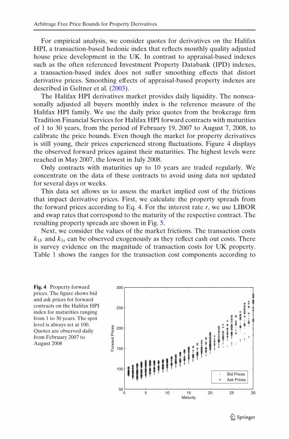
The Halifax HPI derivatives market provides daily liquidity. The nonsea-sonally adjusted all buyers monthly index is the reference measure of theHalifax HPI family. We use the daily price quotes from the brokerage firmTradition Financial Services for Halifax HPI forward contracts with maturitiesof 1 to 30 years, from the period of February 19, 2007 to August 7, 2008, tocalibrate the price bounds. Even though the market for property derivativesis still young, their prices experienced strong fluctuations. Figure 4 displaysthe observed forward prices against their maturities. The highest levels werereached in May 2007, the lowest in July 2008.

Only contracts with maturities up to 10 years are traded regularly. Weconcentrate on the data of these contracts to avoid using data not updatedfor several days or weeks.

This data set allows us to assess the market implied cost of the frictionsthat impact derivative prices. First, we calculate the property spreads fromthe forward prices according to Eq. 4. For the interest rate r, we use LIBORand swap rates that correspond to the maturity of the respective contract. Theresulting property spreads are shown in Fig. 5.

Next, we consider the values of the market frictions. The transaction costsk1b and k1s can be observed exogenously as they reflect cash out costs. Thereis survey evidence on the magnitude of transaction costs for UK property.Table 1 shows the ranges for the transaction cost components according to

Fig. 4 Property forwardprices. The figure shows bidand ask prices for forwardcontracts on the Halifax HPIindex for maturities rangingfrom 1 to 30 years. The spotlevel is always set at 100.Quotes are observed dailyfrom February 2007 toAugust 2008

0 5 10 15 20 25 3050

100

150

200

250

300

Maturity

For

war

d P

rices

Bid PricesAsk Prices

J.M. Syz, P. Vanini

Fig. 5 Observed propertyspreads. The figure showsproperty spreads implied byforward contracts on theHalifax HPI index againstcontract maturity. Quotes areobserved daily from February2007 to August 2008

The Global Property Guide, 2007. Looking for boundary values, we takethe maximum of the ranges. The maximum value of the buyer’s transactioncost range k∗

1b is 5.15% and the maximum value of the seller’s range k∗1s

is 4.11%.To assign a value to the frictions k2 and k3, we fit both the upper and lower

bound to observed prices. In particular, we solve for the boundary values of thefrictions k∗

2 and k∗3 so that the bounds are as narrow as possible but all spread

observations p∗ remain on or within the arbitrage free price bounds. First, k∗2 is

solved by using the formula for the upper bound p, then k∗3 is obtained by using

the formula for the lower bound p. In particular, the minimization problemreads

k∗2 := min{k2 | ∀τ : p∗

τ ≤ pτ (k2)} (7)

respectively

k∗3 := min{k3 | ∀τ : p

τ(k∗

2, k3) ≤ p∗τ }. (8)

This process leads to a market implied cost of 4.48% for transaction timek∗

2 and one of 13.25% for the short sale constraint k∗3. Figure 6 plots the

Table 1 Transaction costs in the UK

Cost component Range Who pays?

Stamp duty 0 to 4% BuyerLegal fees 0.5% to 1% BuyerLand registry fees 0.04% to 0.15% BuyerAgent’s fees 2% to 3.5% (+ 17.5% VAT) SellerCosts paid by buyer 0.54% to 5.15%Costs paid by seller 2.35% to 4.11%Roundtrip transaction costs 2.89% to 9.26%

The Table presents the ranges for real estate transaction cost components as a percentage oftransaction price, according to The Global Property Guide, 2007

Arbitrage Free Price Bounds for Property Derivatives

Fig. 6 Arbitrage free pricebounds. The figure plotshistorical levels of the HalifaxHPI (1983 = 100) and thearbitrage free price boundsfor forward prices of theHalifax HPI index contracts(dashed lines)

1985 1990 1995 2000 2005 2010 2015 20200

200

400

600

800

1000

1200

1400

historical trajectory of the Halifax HPI and the arbitrage free price boundsfor its forward prices by using the obtained values for the market frictions.

Out of Sample Test

The bounds are calibrated using data from February 19, 2007 to August 7, 2008.To challenge the empirical results, we perform an out of sample test with datafrom August 8, 2008 to July 1, 2009.

In particular, we test whether prices obtained in the test period complywith the arbitrage free price bounds for Halifax HPI forward prices. Again,we use daily price quotes from Tradition Financial Services for contracts withmaturities from 1 to 10 years.

Over the whole test period, the upper price bound is never breached. Thelower bound is breached once, in the week of October 28, 2008, when themarket turbulence in the aftermath of the Lehman collapse was at its peak.This breach deserves a closer look.

Our first and most obvious observation is that the breach is ascribed toprice quotes of only two contracts, with 2- and 3-year maturities, respectively.Second, contracts with these maturities were temporarily very illiquid at thattime, which is indicated by quoted bid-ask spreads of over 5%. As we observequoted rather than traded prices, we do not know whether and at what exactprice a trade has actually taken place. Therefore, we perform the calibrationand the out of sample test using mid-prices. These mid-prices might deviateconsiderably from a likely traded price if bid-ask spreads are large, and poten-tially cause a breach of bounds.

Third, the friction costs implied by the quotes that breached the boundsindicate that the breach is very moderate with one exception. The cost oftransaction time k2 never exceeds the boundary value of 4.48%, so no breachoccurs for this friction. The cost of the short sale possibility k3 reaches

J.M. Syz, P. Vanini

a maximum of 13.63% for the 2-year contract and 15.35% for the 3-yearcontract. In comparison to the initial boundary value of 13.25%, the breach ofthe 2-year contract is minor, but the breach of the 3-year contract is substantial.

We identify three potential explanations for the breach of the lower ar-bitrage free price bound: the temporary illiquidity resulting in large bid-askspreads and distorted mid-price quotes; the sample size used for calibration istoo small; or an actual arbitrage opportunity. We consider the temporary illiq-uidity the most straightforward explanation, as the UK real estate market andrelated instruments experienced a general liquidity drought at that time, seee.g. Syz and Vanini (2009). However, to further verify the implied boundaryvalues for the friction costs, we compare our results with other research andmarket observations.

Verification of Friction Costs

The cost of transaction time k2 is a measure of marketability for illiquidassets. Longstaff (1995) derives an analytical upper bound on the value of mar-ketability using option pricing theory. Dyl and Jiang (2008) use the Longstaffmodel to value illiquid common stock. The model requires only two inputs:the volatility of the considered asset and the length of time it’s illiquid or thetime it takes to sell the illiquid asset. The model’s fundamental insight is thatmarketability is properly construed as the option to sell an asset at the timeof one’s own choosing. In particular, Longstaff uses a look-back option thatpays the difference between the maximum asset value during the marketabilityperiod and the asset value at the end of the period. Because a transactionat the maximum value assumes perfect market timing, the option price is anupper bound for the value of marketability. This upper bound is an increasingfunction of the length of the marketability restriction as well as asset volatility.This property is reasonable because the longer it takes to sell an asset and themore volatile its price, then the opportunity cost of not being able to tradebecomes higher. Longstaff mentions that this upper bound can also be viewedas the maximum amount that any investor would be willing to pay to obtainimmediacy in liquidating an asset position. He also assesses whether the boundis consistent with the empirical studies of Pratt (1989) and Silber (1991), whoestimate the value of the lack of marketability of restricted stock and privateequity. He finds that the model can actually provide a tight bound, whichrepresents a useful approximation of the value of marketability. Its closed formsolution is

Dmax =(

2 + σ 2T2

)N(d) +

√σ 2T2π

e− σ2T8 − 1, (9)

where T is the length of the marketability period, σ is the standard deviationof the asset under consideration, N(·) is the cumulative normal distributionfunction and d = √

σ 2T/2.

Arbitrage Free Price Bounds for Property Derivatives

Table 2 Plain and adjusted standard deviations of the Halifax HPI

Sample period Plain standard deviation AR(1) coefficient Adjusted standard deviation

1983–2008 4.55% 0.45 8.28%1991–2008 4.75% 0.39 7.79%1998–2008 5.33% 0.36 8.27%

The first column shows plain standard deviations of the Halifax HPI. The second column showsthe first order autoregressive coefficients of the index; these are used to compute the adjustedstandard deviations presented in the third column. Both plain and adjusted standard deviationsare quoted on an annual basis

The Dmax represents a discount but k2 is a surcharge. The reference valuefor the verification of k∗

2 is thus

k′2 = 1

1 − Dmax− 1. (10)

To apply the Longstaff model to verify k∗2, values for the marketability

period and for the volatility of property are required. According to marketpractice, it takes about 6 months to buy or sell a property as describedabove. Volatility of property indexes needs to be assessed with caution, asproperty prices usually exhibit inertia. Geltner and Miller (2001) propose toadjust standard deviation of property returns by a correction factor equal to1/(1-AR(1)), where AR(1) is the first-order autoregressive coefficient. Wemeasure standard deviation and autocorrelation for the Halifax HPI from itsinception in 1983 to 2008, over the full market cycle from 1991 to 2008 andover the 10-year period from 1998 to 2008. Table 2 summarizes the results.Although plain standard deviation increases and autocorrelation decreasesover time, the adjusted standard deviation turns out to be very stable.

For an illiquidity period of 6 months and an adjusted volatility level over theconsidered market cycle of 7.79% p.a., the Longstaff model gives a value ofk′

2 = 4.68%, as compared to k∗2, which we empirically find to be 4.48%. These

values are very close and indicate a reasonable level.Next, the cost of the short sale constraint k3 has to be verified. The most

direct measure of short sale costs is the lending or loan fee paid by the lenderof a security to the borrower of that security.2 This fee arises because to sella security short, an investor must borrow shares from an investor who ownsthem and is willing to lend them. The lending fee serves to equilibrate supplyand demand in the lending market.

Although quantity data in the shorting market are readily available, pricedata are not. The lending market is not centralized and lending fees do notneed to be disclosed. Cohen et al. (2007) report examples from a sample ofproprietary stock lending data from September 1999 to August 2003. They

2A series of recent papers analyzes direct measures of shorting costs: Brent et al. (1990), D’Avolio(2002), Figlewski and Webb (1993), Lamont and Stein (2004), Ofek et al. (2004), Jones and Lamont(2002), Reed (2002) and Geczy et al. (2002).

J.M. Syz, P. Vanini

report statistics on the full sample and on two subsamples of large stocks andsmall stocks.3 The mean lending fee from the full sample is 2.60% p.a. andthe 0.75 percentile value is at 4.20%. For large stocks, the mean lending feeis 0.39% and the 0.75 percentile value is only at 0.16%. Small stocks on theother hand have much higher loan fees with a mean value at 3.94% and a 0.75percentile value at 5.30%. The most extreme lending fees in this sample are7.25% and 14.75% respectively.

D’Avolio (2002) describes the market for borrowing stock and finds that91% of the stocks lent out in the investigated sample exhibit a lending feebelow 1%. The remaining 9% of the stocks have a mean fee of 4.3%. Less than1% of the sample—typically small stocks with little institutional ownership—exhibit very high fees ranging from 10% up to 79%.

To investigate boundary levels, extreme values that reflect the maximumwillingness to pay for a short sale possibility are critical. Stocks with very highlending fees can be considered special cases. For example, Lamont and Thaler(2003) study 18 equity carve-outs from April 1996 to August 2000 in which theparent has stated its intention to spin off its remaining shares of an alreadylisted subsidiary company. Most subsidiaries were overpriced compared totheir parent companies and had a significantly larger short interest than theparent. In the case of Palm Inc, a temporarily heavily overpriced subsidiary of3Com, short interest was as high as 147.6% at the peak. That is, a numbergreater than all floating shares had been sold short. Borrowed shares canbe sold short to an investor who then lends them again. Lamont and Thaler(2001) conclude that, in the case of Palm, arbitrageurs could not find enoughshares to satisfy the demand of irrational investors. The chief impediment ofthe arbitrage strategy of buying parents and shorting subsidiaries is short saleconstraints.

The value of a short sale opportunity for an index that reflects a broadproperty portfolio cannot be directly compared to the short sale cost of aparticular stock. In sum, the level of typical lending fees is clearly below theobtained boundary value of shorting costs, k∗

3 = 13.25%, but some specialcases can reach levels far beyond this value. The relatively high value of k∗

3might reflect the fact that actual property can be overpriced because of someirrational investors unlike derivatives in which short selling is possible.

Conclusion

Prices of property derivatives do not result from a simple no-arbitrage argu-ment because the derivatives cannot be perfectly replicated. Transaction costs,transaction time, and short sale constraints cause a property spread, whichis a measure for prices in the incomplete real estate market. Because these

3Large stocks exhibit a market capitalization above the NYSE median while small stocks are belowthe median.

Arbitrage Free Price Bounds for Property Derivatives

frictions inhibit perfect replication, they define arbitrage free price bounds forthe property spread.

In this paper, we set up a framework of arbitrage free price bounds forproperty derivatives. Furthermore, we empirically assign values to the marketfrictions, which effect prices of property derivatives or, equivalently, theproperty spread. We base our research on the UK housing market, whereprices for property derivatives are readily available. In particular, we findboundary values of 5.15% for the buyer’s transaction costs, 4.11% for theseller’s transaction costs, 4.48% for transaction time, and 13.25% for the shortsale constraint. These market implied friction costs turn out to be consistentwith other research and market observations, and confirm the accuracy ofour framework. The price process within the price bounds is left for futureresearch.

References

Baran, L., Buttimer, R., & Clark, S. (2008). Calibration of a commodity price model with unob-served factors: The case of real estate index futures. Review of Futures Markets, 16(4), 455–469.

Bjoerk, T., & Clapham, E. (2002). On the pricing of real estate index linked swaps. Journal ofHousing Economics, 11(4), 418–432.

Brent, A., Morse, D., & Stice, E. (1990). Short interest: Explanations and tests. Journal of Financialand Quantitative Analysis, 25, 273–289.

Buttimer, R., Kau, J., & Slawson, V. (1997). A model for pricing securities dependent upon a realestate index. Journal of Housing Economics, 6(1), 16–30.

Cohen, L., Diether, K., & Malloy, C. (2007). Supply and demand shifts in the shorting market.Journal of Finance, 62(5), 2061–2096.

Cunningham, D., & Hendershott, P. (1984). Pricing fha mortgage default insurance. HousingFinance Review, 3, 373–392.

D’Avolio, G. (2002). The market for borrowing stock. Journal of Financial Economics, 66,271–306.

DiPasquale, D., & Wheaton, W. (1996). Urban economics and real estate markets. EnglewoodCliffs: Prentice Hall.

Dyl, E., & Jiang, G. (2008). Valuing illiquid common stock. Financial Analysts Journal, 64(4),40–47.

Figlewski, S., & Webb, G. (1993). Options, short sales, and market completeness. Journal ofFinance, 48, 761–777.

Geczy, C., Musto, D., & Reed, A. (2002). Stocks are special too: An analysis of the equity lendingmarket. Journal of Financial Economics, 66, 241–269.

Geltner, D., & Miller, N. (2001). Commercial real estate analysis and investments. Mason: College.Geltner, D., MacGregor, B., & Schwann, G. (2003). Appraisal smoothing and price discovery in

real estate markets. Urban Studies, 40(5–6), 1047–1064.Jones, C., & Lamont, O. (2002). Short sale constraints and stock returns. Journal of Financial

Economics, 66, 207–239.Lamont, O., & Stein, J. (2004). Aggregate short interest and market valuations. American

Economic Review, 94, 29–32.Lamont, O., & Thaler, R. (2001). Can the market add and subtract? Mispricing in tech stock

carve-outs. NBER Working Paper Series, (8302).Longstaff, F. (1995). How much can marketability affect security values? Journal of Finance, 50(5),

1767–1774.Malatesta, P., & Hess, A. (1986). Discount mortgage financing and housing prices. Housing

Finance Review, 5, 25–41.Miller, E. (1977). Risk, uncertainty, and divergence of opinion. Journal of Finance, 32, 1152–1168.

J.M. Syz, P. Vanini

Ofek, E., Richardson, M., & Whitelaw, R. (2004). Limited arbitrage and short sales restrictions:Evidence from the options markets. Journal of Financial Economics, 74, 305–342.

Patel, K., & Pereira, R. (2008). Pricing property index linked swaps with counterparty default risk.Journal of Real Estate Finance and Economics, 36(1), 5–21.

Pratt, S. P. (1989). Valuing a business: The analysis of closely held companies. Homewood: DowJones-Irwin.

Quigley, J. (2002). Transaction costs and housing markets. In Housing Economics and PublicPolicy (pp. 56–64). Oxford: Blackwell.

Reed, A. (2002). Costly short-selling and stock price adjustment to earnings announcements.Working paper, University of North Carolina.

Silber, W. L. (1991). Discounts on restricted stock: The impact of illiquidity on stock prices.Financial Analysts Journal, 47, 60–64.

Syz, J., & Vanini, P. (2009). Property derivatives and the subprime crisis. Wilmott Journal, 1(3),163–166.

View publication statsView publication stats