Arbitrage Free Implied Volatility Surfaces

Michael Roper∗

School of Mathematics and StatisticsThe University of Sydney

NSW 2006, Australia

michael.roper@sydney.edu.au

26 March, 2010

Abstract

This paper establishes sufficient conditions for an implied volatility sur-face to be free from “static arbitrage”. The conditions are shown to be neces-sary under certain (very mild) conditions.

Application is made to determining whether or not some proposed im-plied volatility smiles are free of static arbitrage.

This paper establishes sufficient and close to necessary conditions for an impliedvolatility surface to be free from static arbitrage. A call price surface is free of staticarbitrage if there can be no arbitrage opportunities trading in the surface. Moreprecisely, a call option price surface (K, τ) 7→ C(K, τ) is free from static arbitrageif and only if there exists a non-negative martingale, say S, such that C(K, τ) =E ((Sτ − K)+) for every K, τ ≥ 0. We then say that an implied volatility surfaceis free from static arbitrage if the call price surface C(K, τ) = CBS(K, τ,Σ(K, τ)) isfree from static arbitrage, where Σ(K, τ) is the implied volatility at strike K andtime to expiry τ, and CBS(K, τ,Σ(K, τ)) is the Black-Scholes price of a K-strike andτ time to expiry option with implied volatility Σ(K, τ).Determining necessary and sufficient conditions for an implied volatility surfaceto be free of (static) arbitrage is important for a number of reasons. Lee (pp. 11–12

∗This research was supported by ARC Discovery Projects DP0881460 and DP0558539.

1

of [Lee05]), for example, lists a number of applications. First, if a “model gen-erates a theoretical [implied volatility surface] that differs qualitatively from em-pirical facts, [then] we have evidence of model misspecification”. Second, “nec-essary conditions on” the implied volatility surface “for the absence of arbitrageprovide[s] consistency checks that can help to reject unsound proposals” for im-plied volatility parameterisations. Also, as noted by Lee (p. 71 of [Lee00]), it isof “benefit to [market] practitioners who seek parameterisations that fit” the mar-ket implied volatility smile. Finally, as noted by Musiela and Rutskowski (see pp.270-271 of [MR05]) and [Dur03], it is an important and open problem in stochas-tic implied volatility modelling since one needs to know how to specify an initialarbitrage free implied volatility surface.Our investigations proceed in a straightforward manner. We first establish neces-sary and sufficient conditions on the call price surface for it to be free of static arbi-trage. We then translate these conditions into conditions on the implied volatilitysurface.Necessary and sufficient conditions on the call price surface for it to be free fromstatic arbitrage are, under various conditions, quite well known. Buehler (see[Bue06]) considers the case of a finite family of strikes and maturities in the callprice surface, Davis and Hobson (see [DH07]) and Carr and Madan (see [CM05])study similar problems, but with a different focus. Cox and Hobson ([CH05])consider a call price surface to be free of static arbitrage if it may be matched by alocal martingale. We do not use this approach because of the problem of impliedvolatility being ill-defined in strictly local martingale models. Durrleman [Dur03]presents a number of necessary call option restrictions and is able to establish suf-ficiency under very strong conditions. The setup closest to ours is that of Follmerand Schied (see [FS04]), although their conditions differ from ours.Various necessary conditions on a surface for it to be an implied volatility surfaceare known, see Lee [Lee05] and, especially, Durrleman [Dur03]. No set of suffi-cient conditions has been presented in the literature. Themain contribution of thispaper is Theorem 2.9 which presents a set of conditions that, if satisfied, certifiesthat a candidate surface is indeed an implied volatility surface free from static ar-bitrage. The other major result of this paper is Theorem 2.15 which shows thatthe set of conditions which we proved were sufficient are, under two weak con-ditions, necessary properties of an implied volatility surface that is free of staticarbitrage.This paper is organised as follows. In the first section, we give the mathematicalsetup. Some elementary properties of convex functions are recalled. In the secondsection, we give necessary and sufficient conditions for a call price surface to be

2

free of static arbitrage. In the third section, we present sufficient conditions for animplied volatility surface to be free of static arbitrage and show that they are nec-essary under certain (very mild) technical conditions. In the final section, we giveexamples of implied volatility smile parameterisations that have been presentedin the literature and show, using our results, that they are not arbitrage-free.

1 Background

1.1 Setup

We assume throughout this paper zero interest rates and dividend yield. We willalso restrict ourselves to non-negative price processes, and assume that we are in aperfectly liquid market for European calls. That is, call option prices for all strikes,K > 0, and maturities, τ ≥ 0, are known in the market. We exclude strike K = 0from this assumption for two reasons. Firstly, it becomes problematic when onedeals with implied volatility parameterised in terms of log moneyness (ln(K/s),s being the stock price). Secondly, it is simple to take the continuous extension ofthe call price surface to [0,∞)× [0,∞), so that there is no real loss of generality insupposing that K > 0.

Definition 1.1. A call price surface parameterised by s is a function

C : [0,∞)× [0,∞) → R

(K, τ) 7→ C(K, τ)

along with a real number s > 0.

It will sometimes be convenient to simply refer to a call price surface parame-terised by s as a call price surface or a call surface.The next definition follows that presented in [CH05] except for our insistence ontrue martingales.

Definition 1.2. There is no static arbitrage in a call price surface C if there exists anon-negative martingale X on some stochastic basis (Ω,F ,F = (Ft)t≥0,P) withC(K, τ) = E ((Xτ − K)+|F0) for each (K, τ) ∈ [0,∞)× [0,∞). In particular, X0 =s, i.e. the current stock price. If such a martingale and probability space exists,then we say that the call price surface is free of static arbitrage.

3

1.2 Auxiliary Facts

Definition 1.3 (Buehler, Definition 2 in [Bue06]). Let µ, ν be two measures definedon (R,B(R)). Then µ is said to precede ν in the Balayage order if and only if

∫

R

f dµ ≤∫

R

f dν

for all convex functions f . This is denoted by µ ν for probability measures withfinite expectation.

Lemma 1.4 (Follmer and Schied, Corollary 2.63 in [FS04]). Let µ, ν be twomeasures defined on (R,B(R)). We have µ ν if and only if

∫

R

(x− K)+µ(dx) ≤∫

R

(x− K)+ν(dx)

for all K ∈ R.

Theorem 1.5 (Kellerer, Theorem 3 in [Kel72]). LetM = (µt)t∈T be a set of probabilitymeasures on (R,B(R)) with finite expectation at each t ∈ T , where T ⊆ [0,∞) is someBorel set. A Markov sub-martingale with marginal distributions µt exists if M is inBalayage order, that is

µt µt′

for all t < t′ with t, t′ ∈ T .

We will need an obvious corollary to Theorem 1.5.

Corollary 1.6. Let M = (µt)t∈T be a set of probability measures on (R,B(R)) withfinite constant expectation for all t ∈ T , where T ⊆ [0,∞) is some Borel set. A Markovmartingale with marginal distributions µt exists ifM is in Balayage order, that is

µt µt′

for all t < t′ with t, t′ ∈ T .

We will also use some elementary properties of convex functions.

Lemma 1.7. Let f : (0,∞) → R be a function that admits a continuous extension, callit g, to [0,∞). We consider the following conditions on f .

(i) f is convex;

4

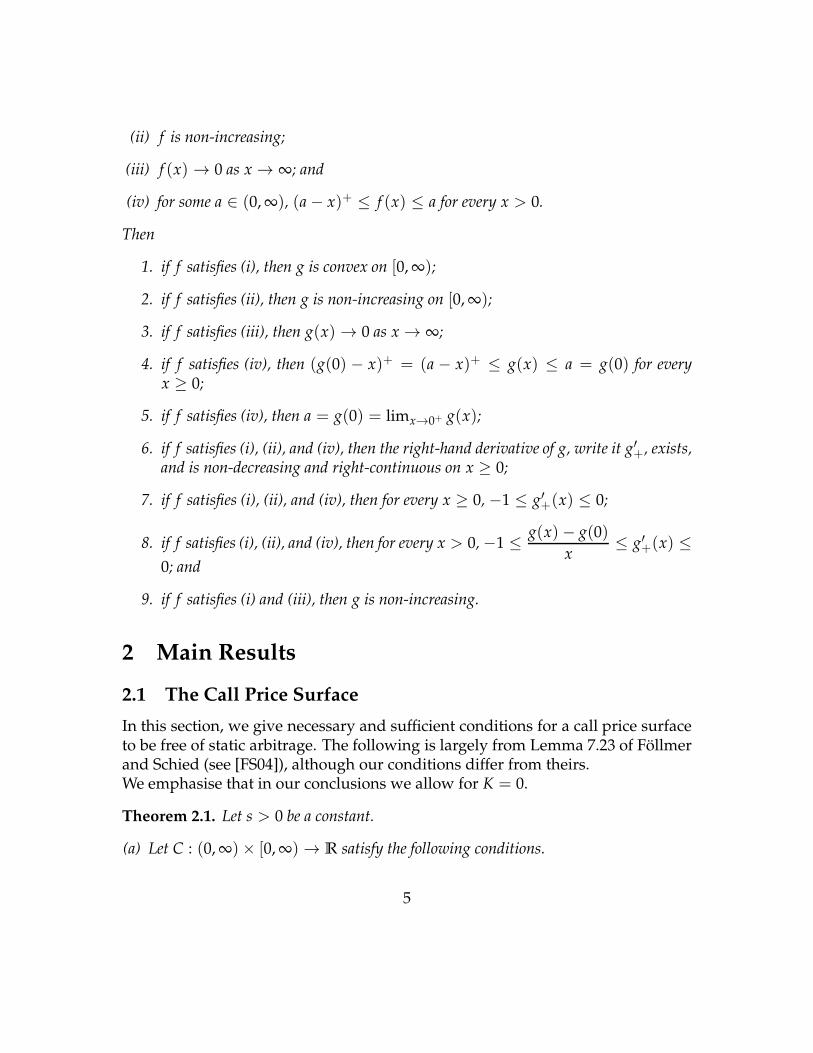
(ii) f is non-increasing;

(iii) f (x) → 0 as x → ∞; and

(iv) for some a ∈ (0,∞), (a− x)+ ≤ f (x) ≤ a for every x > 0.

Then

1. if f satisfies (i), then g is convex on [0,∞);

2. if f satisfies (ii), then g is non-increasing on [0,∞);

3. if f satisfies (iii), then g(x) → 0 as x → ∞;

4. if f satisfies (iv), then (g(0) − x)+ = (a − x)+ ≤ g(x) ≤ a = g(0) for everyx ≥ 0;

5. if f satisfies (iv), then a = g(0) = limx→0+ g(x);

6. if f satisfies (i), (ii), and (iv), then the right-hand derivative of g, write it g′+, exists,and is non-decreasing and right-continuous on x ≥ 0;

7. if f satisfies (i), (ii), and (iv), then for every x ≥ 0, −1 ≤ g′+(x) ≤ 0;

8. if f satisfies (i), (ii), and (iv), then for every x > 0,−1 ≤ g(x)− g(0)

x≤ g′+(x) ≤

0; and

9. if f satisfies (i) and (iii), then g is non-increasing.

2 Main Results

2.1 The Call Price Surface

In this section, we give necessary and sufficient conditions for a call price surfaceto be free of static arbitrage. The following is largely from Lemma 7.23 of Follmerand Schied (see [FS04]), although our conditions differ from theirs.We emphasise that in our conclusions we allow for K = 0.

Theorem 2.1. Let s > 0 be a constant.

(a) Let C : (0,∞)× [0,∞) → R satisfy the following conditions.

5

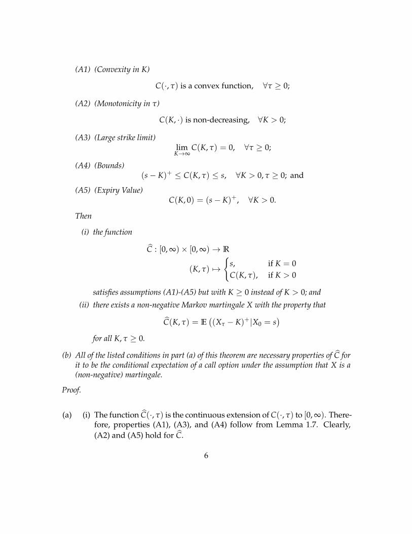
(A1) (Convexity in K)

C(·, τ) is a convex function, ∀τ ≥ 0;

(A2) (Monotonicity in τ)

C(K, ·) is non-decreasing, ∀K > 0;

(A3) (Large strike limit)limK→∞

C(K, τ) = 0, ∀τ ≥ 0;

(A4) (Bounds)(s− K)+ ≤ C(K, τ) ≤ s, ∀K > 0, τ ≥ 0; and

(A5) (Expiry Value)C(K, 0) = (s− K)+, ∀K > 0.

Then

(i) the function

C : [0,∞)× [0,∞) → R

(K, τ) 7→s, if K = 0

C(K, τ), if K > 0

satisfies assumptions (A1)-(A5) but with K ≥ 0 instead of K > 0; and

(ii) there exists a non-negative Markov martingale X with the property that

C(K, τ) = E((Xτ − K)+|X0 = s

)

for all K, τ ≥ 0.

(b) All of the listed conditions in part (a) of this theorem are necessary properties of C forit to be the conditional expectation of a call option under the assumption that X is a(non-negative) martingale.

Proof.

(a) (i) The function C(·, τ) is the continuous extension ofC(·, τ) to [0,∞). There-fore, properties (A1), (A3), and (A4) follow from Lemma 1.7. Clearly,

(A2) and (A5) hold for C.

6

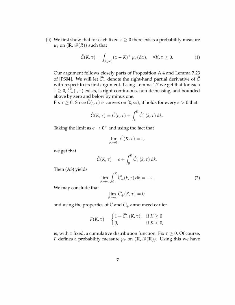
(ii) We first show that for each fixed τ ≥ 0 there exists a probability measureµτ on (R,B(R)) such that

C(K, τ) =∫

[0,∞)(x− K)+ µτ(dx), ∀K, τ ≥ 0. (1)

Our argument follows closely parts of Proposition A.4 and Lemma 7.23

of [FS04]. We will let C′+ denote the right-hand partial derivative of C

with respect to its first argument. Using Lemma 1.7 we get that for each

τ ≥ 0, C′+(·, τ) exists, is right-continuous, non-decreasing, and bounded

above by zero and below by minus one.

Fix τ ≥ 0. Since C(·, τ) is convex on [0,∞), it holds for every ǫ > 0 that

C(K, τ) = C(ǫ, τ) +∫ K

ǫC′+(k, τ)dk.

Taking the limit as ǫ → 0+ and using the fact that

limK→0+

C(K, τ) = s,

we get that

C(K, τ) = s+∫ K

0C′+(k, τ)dk.

Then (A3) yields

limK→∞

∫ K

0C′+(k, τ)dk = −s. (2)

We may conclude that

limK→∞

C′+(K, τ) = 0.

and using the properties of C and C′+ announced earlier

F(K, τ) =

1+ C′

+(K, τ), if K ≥ 0

0, if K < 0,

is, with τ fixed, a cumulative distribution function. Fix τ ≥ 0. Of course,F defines a probability measure µτ on (R,B(R)). Using this we have

7

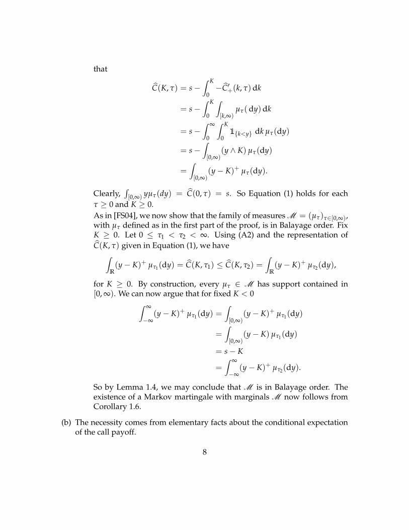
that

C(K, τ) = s−∫ K

0−C′

+(k, τ)dk

= s−∫ K

0

∫

[k,∞)µτ(dy)dk

= s−∫

∞

0

∫ K

01k<y dk µτ(dy)

= s−∫

[0,∞)(y ∧ K) µτ(dy)

=∫

[0,∞)(y− K)+ µτ(dy).

Clearly,∫[0,∞) yµτ(dy) = C(0, τ) = s. So Equation (1) holds for each

τ ≥ 0 and K ≥ 0.

As in [FS04], we now show that the family of measures M = (µτ)τ∈[0,∞),with µτ defined as in the first part of the proof, is in Balayage order. FixK ≥ 0. Let 0 ≤ τ1 < τ2 < ∞. Using (A2) and the representation of

C(K, τ) given in Equation (1), we have∫

R

(y− K)+ µτ1(dy) = C(K, τ1) ≤ C(K, τ2) =∫

R

(y− K)+ µτ2(dy),

for K ≥ 0. By construction, every µτ ∈ M has support contained in[0,∞). We can now argue that for fixed K < 0

∫∞

−∞

(y− K)+ µτ1(dy) =∫

[0,∞)(y− K)+ µτ1(dy)

=∫

[0,∞)(y− K) µτ1(dy)

= s− K

=∫

∞

−∞

(y− K)+ µτ2(dy).

So by Lemma 1.4, we may conclude that M is in Balayage order. Theexistence of a Markov martingale with marginals M now follows fromCorollary 1.6.

(b) The necessity comes from elementary facts about the conditional expectationof the call payoff.

8

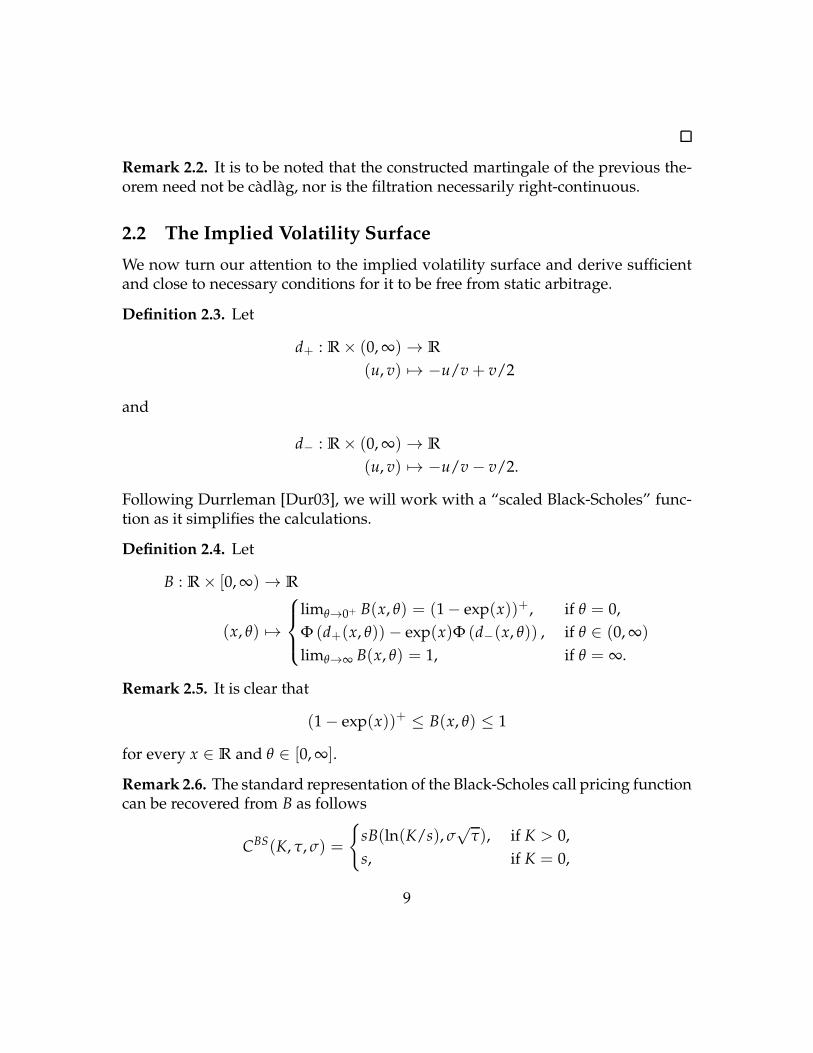
Remark 2.2. It is to be noted that the constructed martingale of the previous the-orem need not be cadlag, nor is the filtration necessarily right-continuous.

2.2 The Implied Volatility Surface

We now turn our attention to the implied volatility surface and derive sufficientand close to necessary conditions for it to be free from static arbitrage.

Definition 2.3. Let

d+ : R × (0,∞) → R

(u, v) 7→ −u/v+ v/2

and

d− : R × (0,∞) → R

(u, v) 7→ −u/v− v/2.

Following Durrleman [Dur03], we will work with a “scaled Black-Scholes” func-tion as it simplifies the calculations.

Definition 2.4. Let

B : R × [0,∞) → R

(x, θ) 7→

limθ→0+ B(x, θ) = (1− exp(x))+ , if θ = 0,

Φ (d+(x, θ))− exp(x)Φ (d−(x, θ)) , if θ ∈ (0,∞)

limθ→∞ B(x, θ) = 1, if θ = ∞.

Remark 2.5. It is clear that

(1− exp(x))+ ≤ B(x, θ) ≤ 1

for every x ∈ R and θ ∈ [0,∞].

Remark 2.6. The standard representation of the Black-Scholes call pricing functioncan be recovered from B as follows

CBS(K, τ, σ) =

sB(ln(K/s), σ

√τ), if K > 0,

s, if K = 0,

9

where s is the current stock price and τ is the time to expiry of the K-strike call.Observe that B is conveniently written solely in terms of log-moneyness, that isln(K/s), and time-scaled volatility σ

√τ.

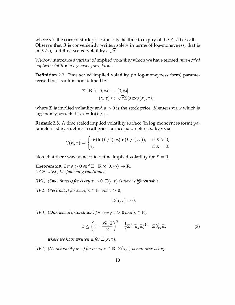
We now introduce a variant of implied volatility which we have termed time-scaledimplied volatility in log-moneyness form.

Definition 2.7. Time scaled implied volatility (in log-moneyness form) parame-terised by s is a function defined by

Ξ : R × [0,∞) → [0,∞]

(x, τ) 7→√

τΣ(s exp(x), τ),

where Σ is implied volatility and s > 0 is the stock price. K enters via x which islog-moneyness, that is x = ln(K/s).

Remark 2.8. A time scaled implied volatility surface (in log-moneyness form) pa-rameterised by s defines a call price surface parameterised by s via

C(K, τ) =

sB(ln(K/s),Ξ(ln(K/s), τ)), if K > 0,

s, if K = 0.

Note that there was no need to define implied volatility for K = 0.

Theorem 2.9. Let s > 0 and Ξ : R × [0,∞) → R.Let Ξ satisfy the following conditions:

(IV1) (Smoothness) for every τ > 0, Ξ(·, τ) is twice differentiable.

(IV2) (Positivity) for every x ∈ R and τ > 0,

Ξ(x, τ) > 0.

(IV3) (Durrleman’s Condition) for every τ > 0 and x ∈ R,

0 ≤(1− x∂xΞ

Ξ

)2

− 1

4Ξ2 (∂xΞ)2 + Ξ∂2xxΞ, (3)

where we have written Ξ for Ξ(x, τ).

(IV4) (Monotonicity in τ) for every x ∈ R, Ξ(x, ·) is non-decreasing.

10

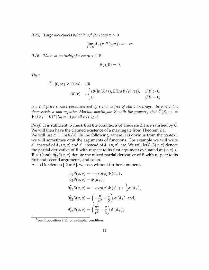
(IV5) (Large moneyness behaviour)1 for every τ > 0

limx→∞

d+(x,Ξ(x, τ)) = −∞.

(IV6) (Value at maturity) for every x ∈ R,

Ξ(x, 0) = 0.

Then

C : [0,∞)× [0,∞) → R

(K, τ) 7→sB(ln(K/s),Ξ(ln(K/s), τ)), if K > 0,

s, if K = 0,

is a call price surface parameterised by s that is free of static arbitrage. In particular,

there exists a non-negative Markov martingale X with the property that C(K, τ) =E ((Xτ − K)+|X0 = s) for all K, τ ≥ 0.

Proof. It is sufficient to check that the conditions of Theorem 2.1 are satisfied by C.We will then have the claimed existence of a martingale from Theorem 2.1.We will use x = ln(K/s). In the following, where it is obvious from the context,we will sometimes omit the arguments of functions. For example we will writed+ instead of d+(u, v) and d− instead of d−(u, v), etc. We will let ∂1B(u, v) denotethe partial derivative of B with respect to its first argument evaluated at (u, v) ∈R × (0,∞), ∂212B(u, v) denote the mixed partial derivative of B with respect to itsfirst and second arguments, and so on.As in Durrleman [Dur03], we use, without further comment,

∂1B(u, v) = − exp(u)Φ (d−) ,∂2B(u, v) = φ (d+) ,

∂211B(u, v) = − exp(u)Φ (d−) +1

vφ (d+) ,

∂212B(u, v) =

(− u

v2+

1

2

)φ (d+) and,

∂222B(u, v) =

(u2

v3− v

4

)φ (d+) ;

1See Proposition 2.11 for a simpler condition.

11

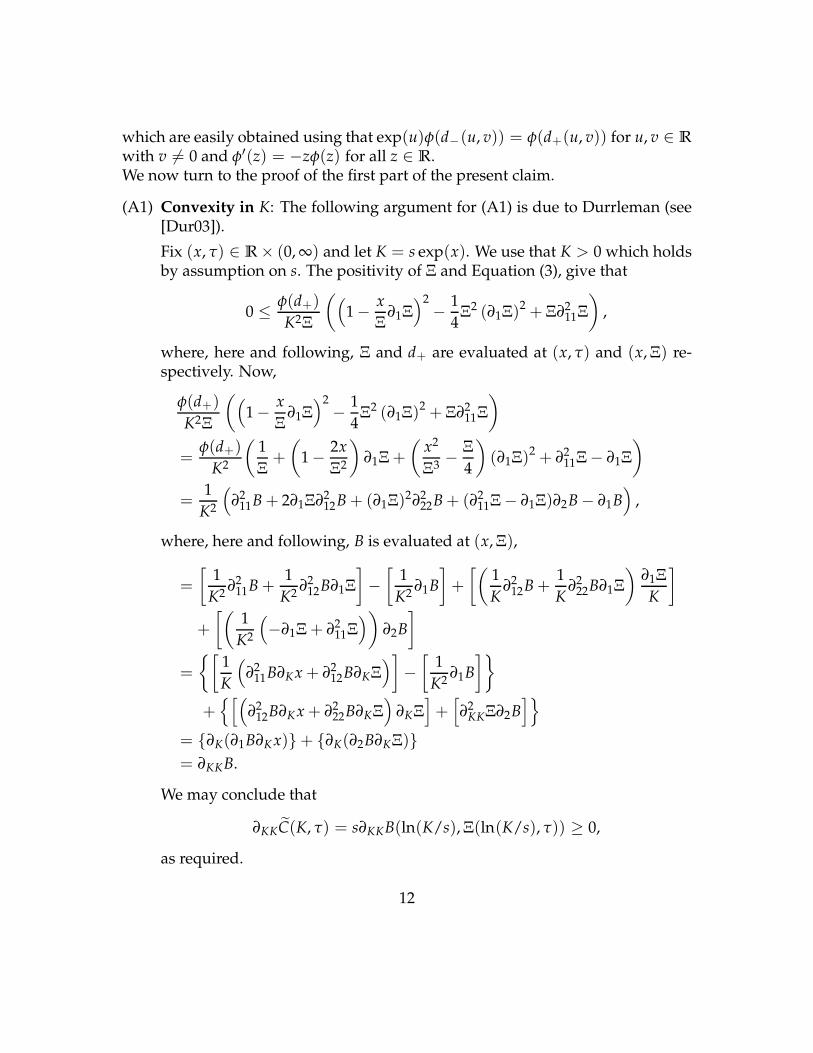
which are easily obtained using that exp(u)φ(d−(u, v)) = φ(d+(u, v)) for u, v ∈ R

with v 6= 0 and φ′(z) = −zφ(z) for all z ∈ R.We now turn to the proof of the first part of the present claim.

(A1) Convexity in K: The following argument for (A1) is due to Durrleman (see[Dur03]).

Fix (x, τ) ∈ R × (0,∞) and let K = s exp(x). We use that K > 0 which holdsby assumption on s. The positivity of Ξ and Equation (3), give that

0 ≤ φ(d+)

K2Ξ

((1− x

Ξ∂1Ξ

)2− 1

4Ξ2 (∂1Ξ)2 + Ξ∂211Ξ

),

where, here and following, Ξ and d+ are evaluated at (x, τ) and (x,Ξ) re-spectively. Now,

φ(d+)

K2Ξ

((1− x

Ξ∂1Ξ

)2− 1

4Ξ2 (∂1Ξ)2 + Ξ∂211Ξ

)

=φ(d+)

K2

(1

Ξ+

(1− 2x

Ξ2

)∂1Ξ +

(x2

Ξ3− Ξ

4

)(∂1Ξ)2 + ∂211Ξ − ∂1Ξ

)

=1

K2

(∂211B+ 2∂1Ξ∂212B+ (∂1Ξ)2∂222B+ (∂211Ξ − ∂1Ξ)∂2B− ∂1B

),

where, here and following, B is evaluated at (x,Ξ),

=

[1

K2∂211B+

1

K2∂212B∂1Ξ

]−[1

K2∂1B

]+

[(1

K∂212B+

1

K∂222B∂1Ξ

)∂1Ξ

K

]

+

[(1

K2

(−∂1Ξ + ∂211Ξ

))∂2B

]

=

[1

K

(∂211B∂Kx+ ∂212B∂KΞ

)]−[1

K2∂1B

]

+[(

∂212B∂Kx+ ∂222B∂KΞ

)∂KΞ

]+[∂2KKΞ∂2B

]

= ∂K(∂1B∂Kx)+ ∂K(∂2B∂KΞ)= ∂KKB.

We may conclude that

∂KKC(K, τ) = s∂KKB(ln(K/s),Ξ(ln(K/s), τ)) ≥ 0,

as required.

12

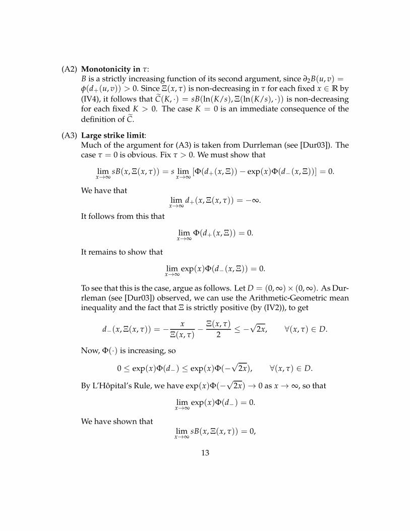
(A2) Monotonicity in τ:B is a strictly increasing function of its second argument, since ∂2B(u, v) =φ(d+(u, v)) > 0. Since Ξ(x, τ) is non-decreasing in τ for each fixed x ∈ R by

(IV4), it follows that C(K, ·) = sB(ln(K/s),Ξ(ln(K/s), ·)) is non-decreasingfor each fixed K > 0. The case K = 0 is an immediate consequence of the

definition of C.

(A3) Large strike limit:Much of the argument for (A3) is taken from Durrleman (see [Dur03]). Thecase τ = 0 is obvious. Fix τ > 0. We must show that

limx→∞

sB(x,Ξ(x, τ)) = s limx→∞

[Φ(d+(x,Ξ))− exp(x)Φ(d−(x,Ξ))] = 0.

We have thatlimx→∞

d+(x,Ξ(x, τ)) = −∞.

It follows from this that

limx→∞

Φ(d+(x,Ξ)) = 0.

It remains to show that

limx→∞

exp(x)Φ(d−(x,Ξ)) = 0.

To see that this is the case, argue as follows. LetD = (0,∞)× (0,∞). As Dur-rleman (see [Dur03]) observed, we can use the Arithmetic-Geometric meaninequality and the fact that Ξ is strictly positive (by (IV2)), to get

d−(x,Ξ(x, τ)) = − x

Ξ(x, τ)− Ξ(x, τ)

2≤ −

√2x, ∀(x, τ) ∈ D.

Now, Φ(·) is increasing, so

0 ≤ exp(x)Φ(d−) ≤ exp(x)Φ(−√2x), ∀(x, τ) ∈ D.

By L’Hopital’s Rule, we have exp(x)Φ(−√2x) → 0 as x → ∞, so that

limx→∞

exp(x)Φ(d−) = 0.

We have shown thatlimx→∞

sB(x,Ξ(x, τ)) = 0,

13

given that d+ → −∞. It follows that

limK→∞

C(K, τ) = 0

when d+ → −∞.

(A4) Bounds:As already noted in Remark 2.5, we have for all x ∈ R and θ ∈ [0,∞] that

(1− exp(x))+ ≤ B(x, θ) ≤ 1.

Multiplying through by s, which is assumed to be positive, and recalling thatx = ln(K/s) we are done.

(A5) Expiry value:Immediate.

The proof is therefore complete.

Remark 2.10. The following proposition delivers a simpler test for the Large mon-eyness behaviour. The test is based on the behaviour ofsef

Ξ(x, τ)√2x

,

for large x. Lee [Lee05] presents his Large moneyness test as Lee requires

lim supx→∞

Ξ(x, τ)√2x

≤ 1

while Durrleman [Dur03] requires

lim supx→∞

Ξ(x, τ)√2x

< 1.

In fact, the case lim supx→∞

Ξ(x, τ)√2x

= 1, requires special treatment as we now see.

Proposition 2.11. We have that

1. d+(x,Ξ(x, τ)) → −∞ when lim supx→∞

Ξ(x, τ)√2x

∈ [0, 1);

14

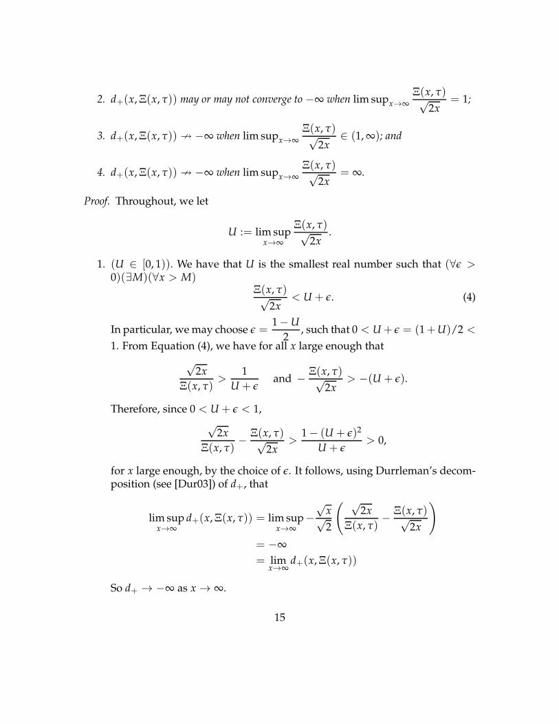
2. d+(x,Ξ(x, τ)) may or may not converge to −∞ when lim supx→∞

Ξ(x, τ)√2x

= 1;

3. d+(x,Ξ(x, τ)) 9 −∞ when lim supx→∞

Ξ(x, τ)√2x

∈ (1,∞); and

4. d+(x,Ξ(x, τ)) 9 −∞ when lim supx→∞

Ξ(x, τ)√2x

= ∞.

Proof. Throughout, we let

U := lim supx→∞

Ξ(x, τ)√2x

.

1. (U ∈ [0, 1)). We have that U is the smallest real number such that (∀ǫ >

0)(∃M)(∀x > M)Ξ(x, τ)√

2x< U + ǫ. (4)

In particular, we may choose ǫ =1−U

2, such that 0 < U+ ǫ = (1+U)/2 <

1. From Equation (4), we have for all x large enough that

√2x

Ξ(x, τ)>

1

U + ǫand − Ξ(x, τ)√

2x> −(U + ǫ).

Therefore, since 0 < U + ǫ < 1,

√2x

Ξ(x, τ)− Ξ(x, τ)√

2x>

1− (U + ǫ)2

U + ǫ> 0,

for x large enough, by the choice of ǫ. It follows, using Durrleman’s decom-position (see [Dur03]) of d+, that

lim supx→∞

d+(x,Ξ(x, τ)) = lim supx→∞

−√x√2

( √2x

Ξ(x, τ)− Ξ(x, τ)√

2x

)

= −∞

= limx→∞

d+(x,Ξ(x, τ))

So d+ → −∞ as x → ∞.

15

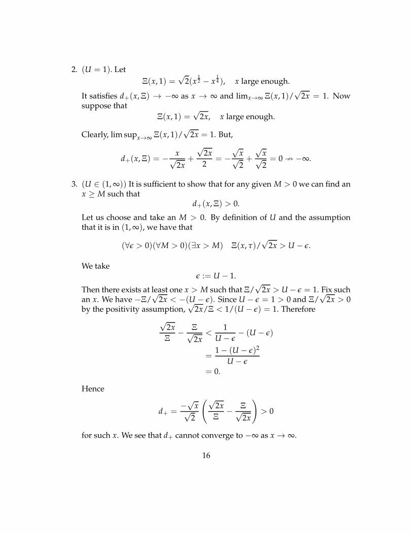
2. (U = 1). Let

Ξ(x, 1) =√2(x

12 − x

14 ), x large enough.

It satisfies d+(x,Ξ) → −∞ as x → ∞ and limx→∞ Ξ(x, 1)/√2x = 1. Now

suppose that

Ξ(x, 1) =√2x, x large enough.

Clearly, lim supx→∞Ξ(x, 1)/

√2x = 1. But,

d+(x,Ξ) = − x√2x

+

√2x

2= −

√x√2+

√x√2= 0 9 −∞.

3. (U ∈ (1,∞)) It is sufficient to show that for any given M > 0 we can find anx ≥ M such that

d+(x,Ξ) > 0.

Let us choose and take an M > 0. By definition of U and the assumptionthat it is in (1,∞), we have that

(∀ǫ > 0)(∀M > 0)(∃x > M) Ξ(x, τ)/√2x > U − ǫ.

We takeǫ := U − 1.

Then there exists at least one x > M such that Ξ/√2x > U− ǫ = 1. Fix such

an x. We have −Ξ/√2x < −(U − ǫ). Since U − ǫ = 1 > 0 and Ξ/

√2x > 0

by the positivity assumption,√2x/Ξ < 1/(U − ǫ) = 1. Therefore

√2x

Ξ− Ξ√

2x<

1

U − ǫ− (U − ǫ)

=1− (U − ǫ)2

U − ǫ

= 0.

Hence

d+ =−√

x√2

(√2x

Ξ− Ξ√

2x

)> 0

for such x. We see that d+ cannot converge to −∞ as x → ∞.

16

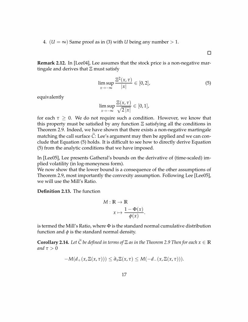
4. (U = ∞) Same proof as in (3) with U being any number > 1.

Remark 2.12. In [Lee04], Lee assumes that the stock price is a non-negative mar-tingale and derives that Ξ must satisfy

lim supx→−∞

Ξ2(x, τ)

|x| ∈ [0, 2], (5)

equivalently

lim supx→−∞

Ξ(x, τ)√2 |x|

∈ [0, 1],

for each τ ≥ 0. We do not require such a condition. However, we know thatthis property must be satisfied by any function Ξ satisfying all the conditions inTheorem 2.9. Indeed, we have shown that there exists a non-negative martingale

matching the call surface C: Lee’s argument may then be applied and we can con-clude that Equation (5) holds. It is difficult to see how to directly derive Equation(5) from the analytic conditions that we have imposed.

In [Lee05], Lee presents Gatheral’s bounds on the derivative of (time-scaled) im-plied volatility (in log-moneyness form).We now show that the lower bound is a consequence of the other assumptions ofTheorem 2.9, most importantly the convexity assumption. Following Lee [Lee05],we will use the Mill’s Ratio.

Definition 2.13. The function

M : R → R

x 7→ 1− Φ(x)

φ(x).

is termed theMill’s Ratio, where Φ is the standard normal cumulative distributionfunction and φ is the standard normal density.

Corollary 2.14. Let C be defined in terms of Ξ as in the Theorem 2.9 Then for each x ∈ R

and τ > 0

−M(d+(x,Ξ(x, τ))) ≤ ∂xΞ(x, τ) ≤ M(−d−(x,Ξ(x, τ))).

17

Proof. We have the bounds (s − K)+ ≤ C(K, τ) ≤ s for each K and τ. For thelower bound we can then use Lemma 1.7 to get that for K > 0

∂KC(K, τ) =s

K(∂1B+ ∂2B∂xΞ)

≥ C(K, τ)− s

K

=sB− s

K

=s(B− 1)

K.

Hence,∂1B+ ∂2B∂xΞ ≥ B− 1,

so that

∂xΞ ≥ B− 1− ∂1B

∂2B

=Φ(d+)− exΦ(d−)− 1+ exΦ(d−)

∂2B

=Φ(d+)− 1

φ(d+)

= −1− Φ(d+)

φ(d+)

= −M(d+).

For the upper boundwe note from Lemma 1.7 that C is non-increasing fromwhich

∂KC ≤ 0

⇔ s

K(∂1B+ ∂2B∂xΞ) ≤ 0

⇔ ∂1B+ ∂2B∂xΞ ≤ 0

⇔ ∂xΞ ≤ −∂1B

∂2B

⇔ ∂xΞ ≤ exΦ(d−)φ(d+)

⇔ ∂xΞ ≤ M(−d−).

18

We now show that the stated conditions are necessary under the smoothness andpositivity requirements to ensure that the resulting call surface is free from staticarbitrage.

Theorem 2.15. Let s > 0 and Ξ : R × [0,∞) → R. Let Ξ satisfy the following condi-tions

(1) (Smoothness) For every τ > 0, Ξ(·, τ) is twice differentiable.

(2) (Positivity) For every x ∈ R and τ > 0,

Ξ(x, τ) > 0.

Let

C : [0,∞)× [0,∞) → R

(K, τ) 7→sB(ln(K/s),Ξ(ln(K/s), τ)), if K > 0,

s, if K = 0.

Then if Ξ violates any of the remaining conditions (IV3)-(IV6) of Theorem 2.9, C is not acall surface free from static arbitrage.

Proof. The necessity of conditions (IV3), (IV4) was shown in Durrleman [Dur03];in fact, the argument is clear by “reversing” the proofs of (A1) and (A2) in Theo-rem 2. Our condition of (IV5) differs from Durrleman’s version of the property inorder to allow for the case

lim supx→∞

Ξ(x, τ)√2x

= 1.

( See Remark 2.11.) The necessity of (IV3) and (IV4) in this paper are taken directlyfrom Durrleman [Dur03]. (Durrleman [Dur03] assumes that (IV1) and (IV2) hold.)With respect to the condition (IV6) we simplify specify the expiry value, whereasDurrleman [Dur03] takes it to be given as the small time expiry.

3 Examples: Parameterisations of the Implied Volatil-

ity Smile

In this section, we investigate whether or not some proposed parameterisationsof the implied volatility smile are arbitrage-free or not. By the implied volatility

19

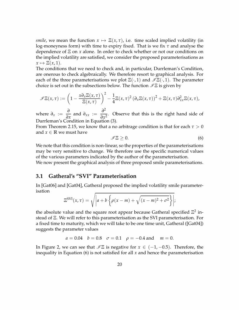
smile, we mean the function x 7→ Ξ(x, τ), i.e. time scaled implied volatility (inlog-moneyness form) with time to expiry fixed. That is we fix τ and analyse thedependence of Ξ on x alone. In order to check whether or not our conditions onthe implied volatility are satisfied, we consider the proposed parameterisations asx 7→ Ξ(x, 1).The conditions that we need to check and, in particular, Durrleman’s Condition,are onerous to check algebraically. We therefore resort to graphical analysis. Foreach of the three parameterisations we plot Ξ(·, 1) and I Ξ(·, 1). The parameterchoice is set out in the subsections below. The function I Ξ is given by

I Ξ(x, τ) :=

(1− x∂xΞ(x, τ)

Ξ(x, τ)

)2

− 1

4Ξ(x, τ)2 (∂xΞ(x, τ))2 + Ξ(x, τ)∂2xxΞ(x, τ),

where ∂x :=∂

∂xand ∂xx :=

∂2

∂x2. Observe that this is the right hand side of

Durrleman’s Condition in Equation (3).From Theorem 2.15, we know that a no arbitrage condition is that for each τ > 0and x ∈ R we must have

I Ξ ≥ 0. (6)

We note that this condition is non-linear, so the properties of the parameterisationsmay be very sensitive to change. We therefore use the specific numerical valuesof the various parameters indicated by the author of the parameterisation.We now present the graphical analysis of three proposed smile parameterisations.

3.1 Gatheral’s “SVI” Parameterisation

In [Gat06] and [Gat04], Gatheral proposed the implied volatility smile parameter-isation

ΞSVI(x, τ) =

√∣∣∣∣a+ b

ρ(x−m) +

√(x−m)2 + σ2

∣∣∣∣;

the absolute value and the square root appear because Gatheral specified Ξ2 in-

stead of Ξ. We will refer to this parameterisation as the SVI parameterisation. Fora fixed time to maturity, which we will take to be one time unit, Gatheral ([Gat04])suggests the parameter values

a = 0.04 b = 0.8 σ = 0.1 ρ = −0.4 and m = 0.

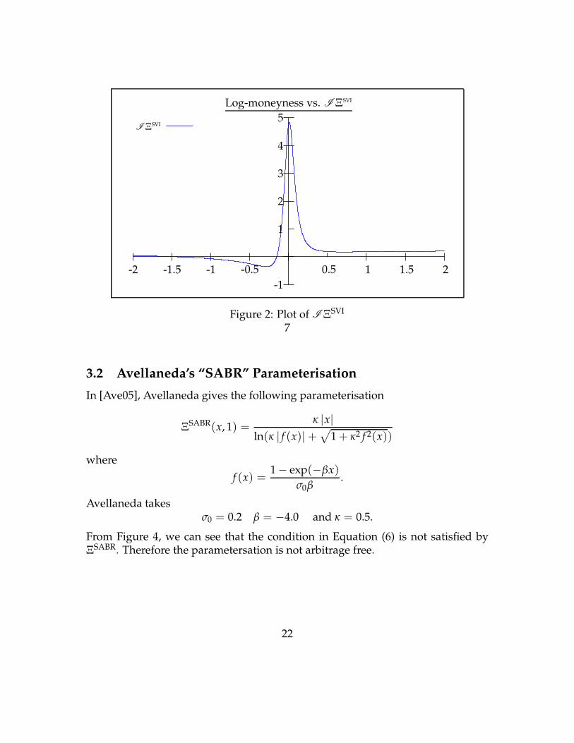
In Figure 2, we can see that I Ξ is negative for x ∈ (−1,−0.5). Therefore, theinequality in Equation (6) is not satisfied for all x and hence the parameterisation

20

is not arbitrage free. (Gatheral’s condition that b(1+ |ρ|) ≤ 4/τ is clearly satisfiedby the parameters we used.)

0.5

1

1.5

2

-1.5 -1 -0.5 0.5 1 1.5

Log-moneyness vs ΞSVI

ΞSVI

Figure 1: Plot of the implied volatility function ΞSVI

21

-1

1

2

3

4

5

-2 -1.5 -1 -0.5 0.5 1 1.5 2

Log-moneyness vs. I ΞSVI

I ΞSVI

Figure 2: Plot of I ΞSVI

7

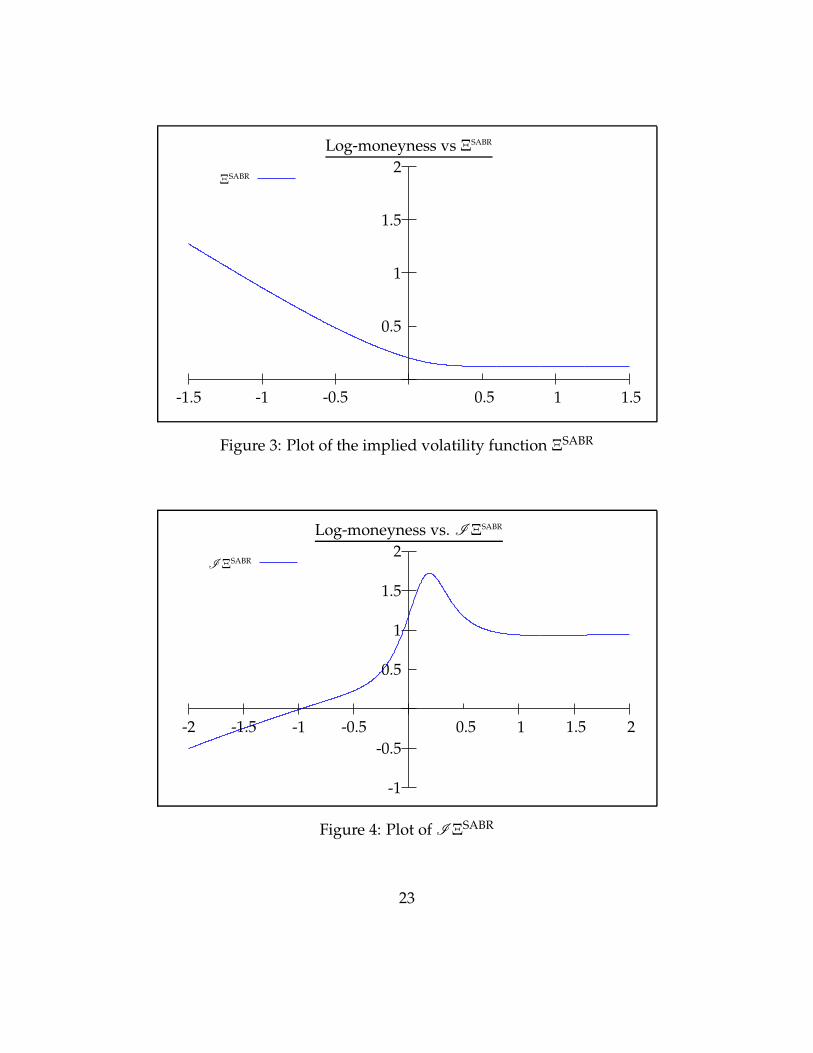
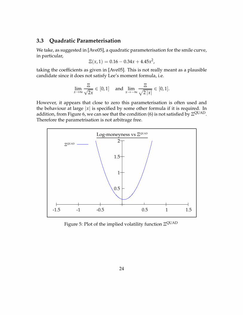
3.2 Avellaneda’s “SABR” Parameterisation

In [Ave05], Avellaneda gives the following parameterisation

ΞSABR(x, 1) =

κ |x|ln(κ | f (x)| +

√1+ κ2 f 2(x))

where

f (x) =1− exp(−βx)

σ0β.

Avellaneda takesσ0 = 0.2 β = −4.0 and κ = 0.5.

From Figure 4, we can see that the condition in Equation (6) is not satisfied byΞSABR. Therefore the parametersation is not arbitrage free.

22

0.5

1

1.5

2

-1.5 -1 -0.5 0.5 1 1.5

Log-moneyness vs ΞSABR

ΞSABR

Figure 3: Plot of the implied volatility function ΞSABR

-1

-0.5

0.5

1

1.5

2

-2 -1.5 -1 -0.5 0.5 1 1.5 2

Log-moneyness vs. I ΞSABR

I ΞSABR

Figure 4: Plot of I ΞSABR

23

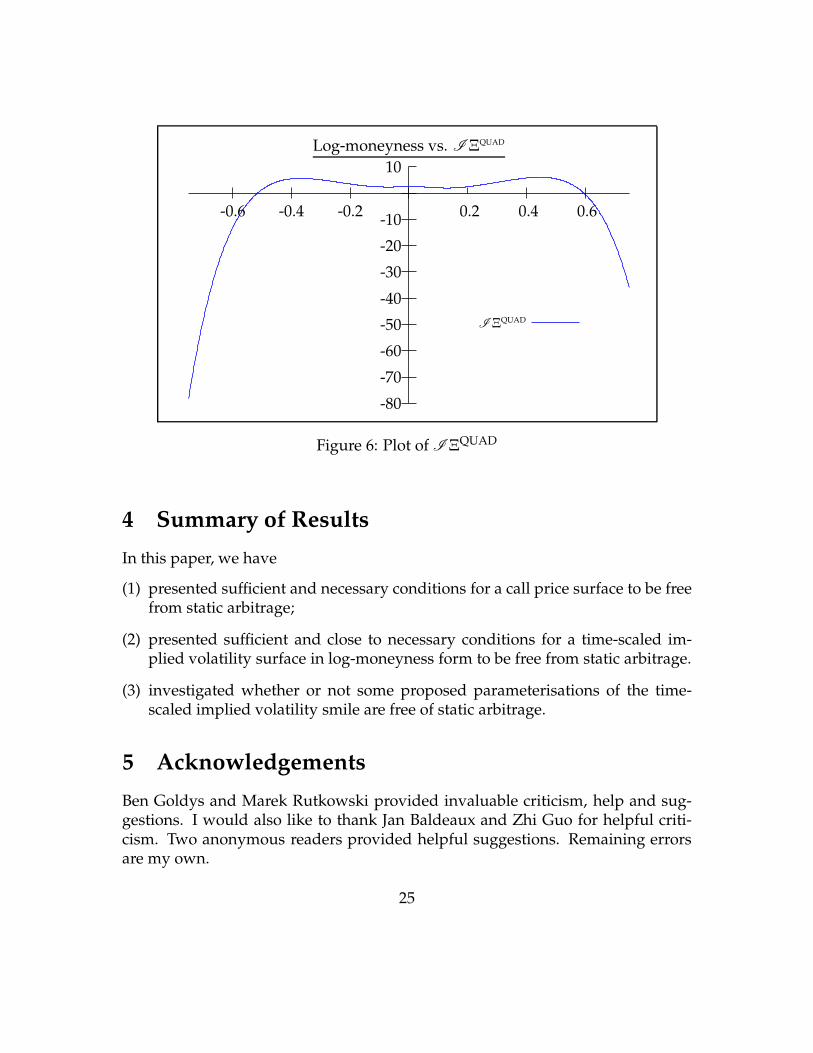
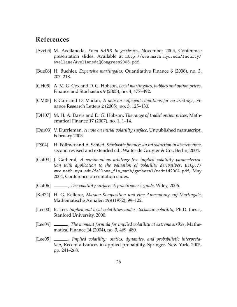
3.3 Quadratic Parameterisation

We take, as suggested in [Ave05], a quadratic parameterisation for the smile curve,in particular,

Ξ(x, 1) = 0.16− 0.34x+ 4.45x2,

taking the coefficients as given in [Ave05]. This is not really meant as a plausiblecandidate since it does not satisfy Lee’s moment formula, i.e.

limx→∞

Ξ√2x

∈ [0, 1] and limx→−∞

Ξ√2 |x|

∈ [0, 1].

However, it appears that close to zero this parameterisation is often used andthe behaviour at large |x| is specified by some other formula if it is required. Inaddition, from Figure 6, we can see that the condition (6) is not satisfied by Ξ

QUAD.Therefore the parametrisation is not arbitrage free.

0.5

1

1.5

2

-1.5 -1 -0.5 0.5 1 1.5

Log-moneyness vs ΞQUAD

ΞQUAD

Figure 5: Plot of the implied volatility function ΞQUAD

24

-80

-70

-60

-50

-40

-30

-20

-10

10

-0.6 -0.4 -0.2 0.2 0.4 0.6

Log-moneyness vs. I ΞQUAD

I ΞQUAD

Figure 6: Plot of I ΞQUAD

4 Summary of Results

In this paper, we have

(1) presented sufficient and necessary conditions for a call price surface to be freefrom static arbitrage;

(2) presented sufficient and close to necessary conditions for a time-scaled im-plied volatility surface in log-moneyness form to be free from static arbitrage.

(3) investigated whether or not some proposed parameterisations of the time-scaled implied volatility smile are free of static arbitrage.

5 Acknowledgements

Ben Goldys and Marek Rutkowski provided invaluable criticism, help and sug-gestions. I would also like to thank Jan Baldeaux and Zhi Guo for helpful criti-cism. Two anonymous readers provided helpful suggestions. Remaining errorsare my own.

25

References

[Ave05] M. Avellaneda, From SABR to geodesics, November 2005, Conferencepresentation slides. Available at http://www.math.nyu.edu/faculty/

avellane/AvellanedaQCongress2005.pdf.

[Bue06] H. Buehler, Expensive martingales, Quantitative Finance 6 (2006), no. 3,207–218.

[CH05] A.M. G. Cox andD. G. Hobson, Local martingales, bubbles and option prices,Finance and Stochastics 9 (2005), no. 4, 477–492.

[CM05] P. Carr and D. Madan, A note on sufficient conditions for no arbitrage, Fi-nance Research Letters 2 (2005), no. 3, 125–130.

[DH07] M. H. A. Davis and D. G. Hobson, The range of traded option prices, Math-ematical Finance 17 (2007), no. 1, 1–14.

[Dur03] V. Durrleman, A note on initial volatility surface, Unpublished manuscript,February 2003.

[FS04] H. Follmer andA. Schied, Stochastic finance: an introduction in discrete time,second revised and extended ed., Walter de Gruyter & Co., Berlin, 2004.

[Gat04] J. Gatheral, A parsimonious arbitrage-free implied volatility parameteriza-tion with application to the valuation of volatility derivatives, http://

www.math.nyu.edu/fellows_fin_math/gatheral/madrid2004.pdf, May2004, Conference presentation slides.

[Gat06] , The volatility surface: A practitioner’s guide, Wiley, 2006.

[Kel72] H. G. Kellerer, Markov-Komposition und eine Anwendung auf Martingale,Mathematische Annalen 198 (1972), 99–122.

[Lee00] R. Lee, Implied and local volatilities under stochastic volatility, Ph.D. thesis,Stanford University, 2000.

[Lee04] , The moment formula for implied volatility at extreme strikes, Mathe-matical Finance 14 (2004), no. 3, 469–480.

[Lee05] , Implied volatility: statics, dynamics, and probabilistic interpreta-tion, Recent advances in applied probability, Springer, New York, 2005,pp. 241–268.

26

[MR05] M. Musiela and M. Rutkowski, Martingale methods in financial modelling,2nd ed., vol. 36, Springer-Verlag, Berlin, 2005.

27