ArbeitsberichtNAB 10-21

August 2011

D. Meier, M. Mazurek

Ancillary rock and pore water studies on drillcores from northern

Switzerland

Nationale Genossenschaftfür die Lagerung

radioaktiver Abfälle

Hardstrasse 73CH-5430 Wettingen

Telefon 056-437 11 11

www.nagra.ch

Rock-Water InteractionInstitute of Geological Sciences

University of Bern

KEYWORDS

Tracer profiles, Chloride, Mineralogy, Porosity, Chlorid, Mineralogie, Porosität, Benken, Riniken, Schafisheim,

Weiach, Opalinuston, Effinger Schichten, Brauner Dogger

ArbeitsberichtNAB 10-21

Nationale Genossenschaftfür die Lagerung

radioaktiver Abfälle

Hardstrasse 73CH-5430 Wettingen

Telefon 056-437 11 11

www.nagra.ch

August 2011

D. Meier, M. Mazurek

Ancillary rock and pore water studies on drillcores from northern

Switzerland

Rock-Water InteractionInstitute of Geological Sciences

University of Bern

Nagra Working Reports concern work in progress that may have had limited review. They are

intended to provide rapid dissemination of information. The viewpoints presented and

conclusions reached are those of the author(s) and do not necessarily represent those of

Nagra.

"Copyright © 2011 by Nagra, Wettingen (Switzerland) / All rights reserved.

All parts of this work are protected by copyright. Any utilisation outwith the remit of the

copyright law is unlawful and liable to prosecution. This applies in particular to translations,

storage and processing in electronic systems and programs, microfilms, reproductions, etc."

I NAGRA NAB 10-21

Table of contents

Table of contents ............................................................................................................................ I

List of Tables............................................................................................................................... III

List of Figures ...............................................................................................................................V

1 Introduction............................................................................................................................. 1

2 Sampling ................................................................................................................................. 4

2.1 System geometry.................................................................................................................. 4

2.2 Sampling strategy .............................................................................................................. 10

2.3 Sample selection ................................................................................................................ 11

3 Methods ................................................................................................................................ 12

3.1 Sample preparation ............................................................................................................ 12

3.2 Densities / Porosity ............................................................................................................ 12

3.2.1 Bulk dry density.....................................................................................................................12 3.2.2 Grain density..........................................................................................................................12 3.2.3 Physical porosity....................................................................................................................13

3.3 Mineralogy......................................................................................................................... 13

3.3.1 Whole-rock mineralogy by X-ray diffraction ........................................................................13 3.3.2 Clay mineralogy by X-ray diffraction....................................................................................14 3.3.3 CS-Mat IR spectroscopy........................................................................................................14

3.4 Aqueous extraction ............................................................................................................ 15

4 Results ................................................................................................................................ 16

4.1 Mineralogical composition ................................................................................................ 19

4.2 Densities and physical porosity ......................................................................................... 24

4.3 Anion concentrations ......................................................................................................... 27

5 Derivation of pore-water concentrations of anions: Analysis of methodological approaches based on data from the Benken borehole............................................. 32

5.1 Formalism .......................................................................................................................... 32

5.2 Methods to constrain physical porosity ............................................................................. 32

5. 3 Approaches to defining the anion-accessible porosity fraction ........................................ 33

5.4 Analysis of methods to derive physical and anion-accessible porosity ............................. 34

5.4.1 Porosity calculated from measured bulk dry and grain densities and from gravimetric water loss 34 5.4.2 Porosity calculated from RHOB density log.........................................................................38 5.4.3 Porosity calculated from clay-mineral content .....................................................................38 5.4.4 Evaluation of methods to constrain porosity.........................................................................39

5.5 Conclusions for the calculation of pore-water concentrations of solutes........................... 40

6 Calculated pore-water concentrations of Cl- in all boreholes ............................................... 45

6.1 Analysis of errors and error propagation ........................................................................... 45

6.1.1 Porosity obtained from density measurements ......................................................................45

II NAGRA NAB 10-21

6.1.2 Porosity obtained by regression to clay-mineral content .......................................................45 6.1.3 Calculation of total errors ......................................................................................................46

6.2 Calculated Cl- concentrations in pore water and data screening........................................ 47

6.3 Conclusions........................................................................................................................ 48

7 References............................................................................................................................. 59

III NAGRA NAB 10-21

List of Tables

Tab. 1: Definition of the top and bottom boundaries of the low-permeability sequences in boreholes Benken, Riniken, Schafisheim and Weiach ......................................... 5

Tab. 2: Hydrogeological and hydrochemical information for borehole Benken: Documentation of packer-test intervals, hydraulic conductivities and ground-water compositions in aquifers (from Nagra 2001). The low-permeability sequence is shown in grey, directly embedding aquifers in blue. Further tests and water samples shown in white ........................................................................... 6

Tab. 3: Hydrogeological and hydrochemical information for borehole Riniken: Documentation of packer-test intervals, hydraulic conductivities and ground-water compositions in aquifers (from Nagra 1990). The low-permeability sequence is shown in grey, directly embedding aquifers in blue. Further tests and water samples shown in white ........................................................................... 7

Tab. 4: Hydrogeological and hydrochemical information for borehole Schafisheim: Documentation of packer-test intervals, hydraulic conductivities and ground-water compositions in aquifers (from Nagra 1992). The low-permeability sequence is shown in grey, directly embedding aquifers in blue. Further tests and water samples shown in white ........................................................................... 8

Tab. 5: Hydrogeological and hydrochemical information for borehole Weiach: Documentation of packer-test intervals, hydraulic conductivities and ground-water compositions in aquifers (from Nagra 1989). The low-permeability sequence is shown in grey, directly embedding aquifers in blue. Further tests and water samples shown in white ........................................................................... 9

Tab. 6: Benken: List of samples and lithological classification according to the scheme of Füchtbauer (1988), based on the instrumental mineralogical analyses (see below) ..................................................................................................................... 16

Tab. 7: Riniken: List of samples and lithological classification according to the scheme of Füchtbauer (1988), based on the instrumental mineralogical analyses (see below) ..................................................................................................................... 16

Tab. 8: Schafisheim: List of samples and lithological classification according to the scheme of Füchtbauer (1988), based on the instrumental mineralogical analyses (see below) ............................................................................................... 17

Tab. 9: Weiach: List of samples and lithological classification according to the scheme of Füchtbauer (1988), based on the instrumental mineralogical analyses (see below) ..................................................................................................................... 18

Tab. 10: Benken: Results of mineralogical analyses ............................................................... 19

Tab. 11: Riniken: Results of mineralogical analyses............................................................... 20

Tab. 12: Schafisheim: Results of mineralogical analyses........................................................ 20

Tab. 13: Weiach: Results of mineralogical analyses ............................................................... 21

Tab. 14: Benken: Results of analyses of clay mineralogy ....................................................... 23

Tab. 15: Weiach: Results of analyses of clay mineralogy ....................................................... 23

Tab. 16: Benken: Densities and physical porosity................................................................... 24

Tab. 17: Riniken: Densities and physical porosity .................................................................. 25

IV NAGRA NAB 10-21

Tab. 18: Schafisheim: Densities and physical porosity ........................................................... 26

Tab. 19: Weiach: Densities and physical porosity................................................................... 27

Tab. 20: Benken: Anion concentration in aqueous leachate solutions..................................... 28

Tab. 21: Riniken: Anion concentration in aqueous leachate solutions .................................... 28

Tab. 22: Schafisheim: Anion concentration in aqueous leachate solutions ............................. 29

Tab. 23: Weiach: Anion concentration in aqueous leachate solutions..................................... 30

Tab. 24: Methods to constrain physical porosity in the present study ..................................... 33

Tab. 25: Comparison of porosities of Benken drillcores (Jurassic section) derived from different methods.................................................................................................... 35

Tab. 26: Pore-water chloride contents calculated from aqueous-leaching data of Benken samples using a set of alternative assumptions regarding porosity ........................ 41

Tab. 27: Definition and quantification of errors of parameters that are used to calculate pore-water concentrations of solutes ...................................................................... 46

Tab. 28: Calculated pore-water concentrations of Cl- for the Benken profile ......................... 50

Tab. 29: Calculated pore-water concentrations of Cl- for the Riniken profile......................... 50

Tab. 30: Calculated pore-water concentrations of Cl- for the Schafisheim profile.................. 51

Tab. 31: Calculated pore-water concentrations of Cl- for the Weiach profile ......................... 52

V NAGRA NAB 10-21

List of Figures

Fig. 1: Geological profile of the Benken borehole, including the distinction of aquifers and low-permeability sequences in the Jurassic and Triassic (adapted from Nagra 2001) .............................................................................................................. 2

Fig. 2: Potential siting areas and host rocks for geological disposal of high-level (HAA) and low- and intermediate-level (SMA) radioactive waste in Switzerland (adapted from Nagra 2008). Locations of boreholes studied here are shown in blue...................................................................................................... 3

Fig. 3: Schematic sections of boreholes Benken, Riniken, Schafisheim and Weiach, showing the hydrogeological properties and the sampling positions ..................... 10

Fig. 4: Sample BEN 407.38, consisting of a layer of argillaceous material within limestone beds. Width of photograph is 20 cm ...................................................... 11

Fig. 5: Mineralogy in a ternary plot after Füchtbauer (1988) .................................................. 22

Fig. 6: Cl- vs. Br- contents in aqueous leachates ...................................................................... 31

Fig. 7: Hypotheses relating the anion-accessible porosity fraction to clay-mineral content .................................................................................................................... 34

Fig. 8: Comparison of porosities of Benken drillcores (Jurassic section) derived from different methods (based on data from Tab. 25)..................................................... 37

Fig. 9: Correlation of clay-mineral contents and porosities of the Jurassic sections in boreholes Benken and Weiach................................................................................ 39

Fig. 10: Chloride contents from aqueous leaching of Benken samples recalculated to pore-water contents without any correction for the anion-accessible porosity fraction.................................................................................................................... 42

Fig. 11: Chloride contents from aqueous leaching of Benken samples recalculated to pore-water contents, considering a scaling factor of 0.5 for the anion-accessible porosity fraction in samples with >10 wt.-% clay-mineral content....... 43

Fig. 12: Chloride contents from aqueous leaching of Benken samples recalculated to pore-water contents, considering a mineralogy-dependent scaling factor for the anion-accessible porosity fraction (see text)..................................................... 44

Fig. 13: Cl- profile for Benken using physical porosity for the recalculation to pore-water concentrations ............................................................................................... 53

Fig. 14: Cl- profile for Benken using porosity derived from clay-mineral content for the recalculation to pore-water concentrations ............................................................. 53

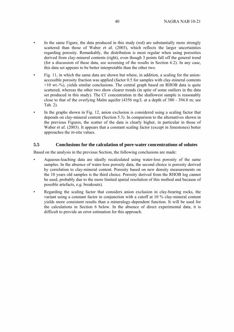
Fig. 15: Cl- profile for Riniken using physical porosity for the recalculation to pore-water concentrations ............................................................................................... 54

Fig. 16: Cl- profile for Riniken using porosity derived from clay-mineral content for the recalculation to pore-water concentrations ............................................................. 54

Fig. 17: Cl- profile for Schafisheim using physical porosity for the recalculation to pore-water concentrations....................................................................................... 55

Fig. 18: Cl- profile for Schafisheim using porosity derived from clay-mineral content for the recalculation to pore-water concentrations ................................................. 55

VI NAGRA NAB 10-21

Fig. 19: Cl- for profile Weiach using physical porosity for the recalculation to pore-water concentrations ............................................................................................... 56

Fig. 20: Cl- profile for Weiach using porosity derived from clay-mineral content for the recalculation to pore-water concentrations ............................................................. 56

Fig. 21: Screened Cl- profile for Benken using porosity derived from clay-mineral content for the recalculation to pore-water concentrations..................................... 57

Fig. 22: Screened Cl- profile for Riniken using porosity derived from clay-mineral content for the recalculation to pore-water concentrations..................................... 57

Fig. 23: Screened Cl- profile for Schafisheim using porosity derived from clay-mineral content for the recalculation to pore-water concentrations..................................... 58

Fig. 24: Screened Cl- profile for Weiach using porosity derived from clay-mineral content for the recalculation to pore-water concentrations..................................... 58

1 NAGRA NAB 10-21

1 Introduction

A laterally extended, about 300 - 600 m thick low-permeability sequence mainly dominated by clay-rich lithologies occurs between the Malm and Triassic (Keuper or Muschelkalk) aquifers of northern Switzerland (an example is provided in Fig. 1). It includes, among other units, three formations that have been proposed by Nagra (2008) as host rocks for various types of radioactive wastes. The five potential siting regions in northern Switzerland and the corresponding host rocks (Opalinus Clay, the overlying "Brauner Dogger"1 and the Effinger Schichten) are shown in Fig. 2.

This report revisits existing drillcore materials from older boreholes in the region of interest and documents the results of a new analytical campaign. The objectives were to study the spatial distribution of natural-tracer concentrations in pore water at locations where this has not been done previously and to augment the mineralogical data base with respect to the newly proposed host rocks "Brauner Dogger" and Effinger Schichten. The present report has the focus on the tracer profiles. The mineralogical data of the host-rock sections are analysed in Mazurek (2011).

One of the motivations for this report was the success of the campaign for the Benken borehole, where regular profiles of Cl-, 18O and 2H were identified across the whole low-permeability sequence (Gimmi & Waber 2004, Gimmi et al. 2007). In that campaign, the tracer profiles, together with the known tracer concentrations in the bounding aquifers and palaeo-hydrogeological constraints, were subjected to transport modelling, in order to reproduce the observed profiles using plausible transport parameters and evolution scenarios. That study, together with a suite of studies related to other European sites (Mazurek et al. 2009, 2011), provided valuable information pertaining to transport mechanisms and parameters and thereby yielded constraints with regard to the long-term evolution of low-permeability sequences.

In this study, core materials from the low-permeability sequence illustrated in Fig. 1 have been sampled in the boreholes of Weiach (WEI; Matter et al. 1988a, Nagra 1989), Riniken (RIN; Matter et al. 1987, Nagra 1990) and Schafisheim (SHA; Matter et al. 1988b, Nagra 1992), together with additional materials from the Benken borehole (BEN; Nagra 2001). Given the fact that the original pore water is no longer present in these core materials, the spectrum of tracers that could be studied was limited to Cl- and Br-. These precipitated as salts when the pore water evaporated but are still present in the rock, unaffected by the environmental conditions during core storage (air humidity, oxidising regime).

1 Definition according to Nagra (2008): The informal term "Brauner Dogger“ relates to the suite of generally clay-

rich rock units stratigraphically located between the Opalinus Clay and the Malm. In the Geological Atlas of Switzerland, these units are shown in brown colours and occur in the Tabular Jura east of the Aare river and the region Zürich-Nordost-Schaffhausen.

2 NAGRA NAB 10-21

Fig. 1: Geological profile of the Benken borehole, including the distinction of aquifers and low-permeability sequences in the Jurassic and Triassic (adapted from Nagra 2001) The exact position of the aquifer horizons varies over the region of interest

3 NAGRA NAB 10-21

Fig. 2: Potential siting areas and host rocks for geological disposal of high-level (HAA) and low- and intermediate-level (SMA) radioactive waste in Switzerland (adapted from Nagra 20082). Locations of boreholes studied here are shown in blue

2 The nomenclature of the potential siting areas has recently been updated: Zürcher Weinland Zürich Nordost,

Nördlich Lägeren Nördlich Lägern, Bözberg Jura Ost.

4 NAGRA NAB 10-21

2 Sampling

2.1 System geometry

The sequences in Benken and Weiach are bounded by the overlying Malm aquifer constituted of massive limestones. In Riniken, these limestones are missing due to erosion, and the base of the Quaternary is considered as the upper boundary. In Schafisheim, a water sample was taken in the Lower Fresh-Water Molasse in the interval 553 - 563 m. In the footwall of this test, no hydraulic data are available down to the top of the Sowerbyi-Sauzei-Schichten, so the upper boundary cannot be clearly defined. The likely spectrum for its position extends from the base of the Molasse interval from which water was produced (563 m) to the base of the Hauptrogenstein (917 m).

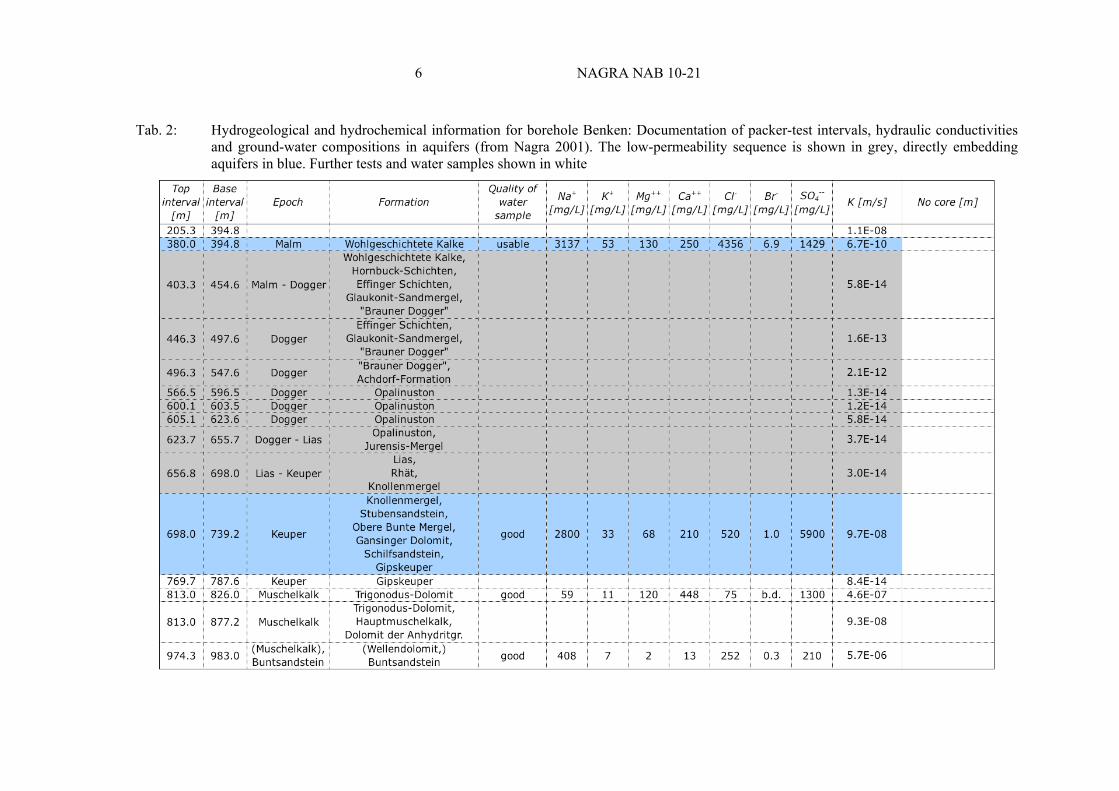
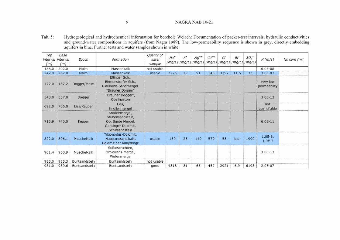
The lower boundary in Benken is constituted of Keuper sandstones. In Riniken, these strata are also taken as the lower boundary, in spite of the lower hydraulic conductivity of 5E-9 m/s in this borehole. In Weiach and Schafisheim, the Keuper has very low hydraulic conductivities. Therefore, the underlying Muschelkalk aquifer is thought to constitute the lower boundary at these sites.

The way the boundaries were defined on the basis of geological information, packer-test results and fluid logs is documented in Tab. 1. In Tab. 2 - 5, the results of pertinent hydraulic tests are summarised, together with information on the chemical composition of ground-water samples taken from the aquifers that embed the low-permeability sequence.

5 NAGRA NAB 10-21

Tab. 1: Definition of the top and bottom boundaries of the low-permeability sequences in boreholes Benken, Riniken, Schafisheim and Weiach

Upper boundary of low-permeability sequence

[m] Lower boundary of low-

permeability sequence [m] Remarks

Missing core section

in low-permeabil-

ity sequence

[m] Benken (BEN)

397 Basis of major subvertical fracture im Malm limestone from which a water sample was pumped (test M2: 380.0 - 394.8 m)

709.1 Top of porous and brecciated sandstone from which a water sample was pumped in the Keuper (test K2: 698.0 - 739.2 m)

-

Riniken (RIN)

25.1 Base Quaternary (overlying Effinger Schichten). No packer tests down to 217 m, but no discontinuities in fluid logs at shallow level (Nagra 1988, Beilage 6.1)

513 Packer test 501 - 530.5 m; no discontinuities in fluid logs (Nagra 1988, Beilage 6.1). Depth of 513 m corresponds to the top of the uppermost sandstone within the Schilfsandstein-Formation

Core section within the low-permeability sequence is

incomplete

33 - 325.4, 490.2 - 513

Schafisheim (SHA)

563 - 917

Base of packer test in USM (Lower Fresh-water Molasse) to base of Hauptrogenstein (exact position unknown due to absence of hydraulic data)

1227 Discontinuities in fluid logs at 1227, 1236 m (top Muschelkalk; see Nagra 1988, Beilage 7.2)

Keuper "aquifer" has low permeability, the low-permeability sequence reaches down to the

Muschelkalk. Core section within the low-permeability

sequence is incomplete

563 - 577, 594.8 - 964

Weiach (WEI)

267 No discontinuities in fluid logs; boundary taken as the base of the packer test in the Malm

822 Packer test 822 - 896.1 m (Muschelkalk); discontinuitues in fluid logs at 822 m (el. conductivity) and 827 m (temperature) (Nagra 1988, Beilage 5.2)

Keuper "aquifer" has low permeability, the low-permeability sequence reaches down to the

Muschelkalk

-

6 NAGRA NAB 10-21

Tab. 2: Hydrogeological and hydrochemical information for borehole Benken: Documentation of packer-test intervals, hydraulic conductivities and ground-water compositions in aquifers (from Nagra 2001). The low-permeability sequence is shown in grey, directly embedding aquifers in blue. Further tests and water samples shown in white

7 NAGRA NAB 10-21

Tab. 3: Hydrogeological and hydrochemical information for borehole Riniken: Documentation of packer-test intervals, hydraulic conductivities and ground-water compositions in aquifers (from Nagra 1990). The low-permeability sequence is shown in grey, directly embedding aquifers in blue. Further tests and water samples shown in white

8 NAGRA NAB 10-21

Tab. 4: Hydrogeological and hydrochemical information for borehole Schafisheim: Documentation of packer-test intervals, hydraulic conductivities and ground-water compositions in aquifers (from Nagra 1992). The low-permeability sequence is shown in grey, directly embedding aquifers in blue. Further tests and water samples shown in white

9 NAGRA NAB 10-21

Tab. 5: Hydrogeological and hydrochemical information for borehole Weiach: Documentation of packer-test intervals, hydraulic conductivities and ground-water compositions in aquifers (from Nagra 1989). The low-permeability sequence is shown in grey, directly embedding aquifers in blue. Further tests and water samples shown in white

10 NAGRA NAB 10-21

2.2 Sampling strategy

Over the entire low-permeability sequences in boreholes Benken, Riniken, Schafisheim and Weiach, the objective was to take a sample approximately every 10 m along hole. In practice, there were the following deviations from this principle:

• In boreholes Riniken and Schafisheim, core materials are not available from parts of the depth intervals of interest (Tab. 3 - 4, Fig. 3). The biggest gaps are in the upper part of the low-permeability sequence.

• Borehole Benken has been studied in detail previously (Nagra 2001, Gimmi & Waber 2004, Gimmi et al. 2007). Sampling for this study was limited to the "Brauner Dogger" (in order to increase the data base from this somewhat heterogeneous sequence) and to the lowermost part of the Malm (from which no samples had been taken previously).

• In the Weiach core, a set of 19 samples between the upper Keuper and the "Brauner Dogger" has been studied by H. N. Waber in 2000 (mineralogy, anion contents based on aqueous extracts; undocumented work). These data were integrated into the present work without re-sampling this interval, with the exception of 3 new samples that were taken to obtain an even denser coverage of the profile.

Finally, a total of 94 samples were collected for this study.

Fig. 3: Schematic sections of boreholes Benken, Riniken, Schafisheim and Weiach, showing the hydrogeological properties and the sampling positions

11 NAGRA NAB 10-21

2.3 Sample selection

Samples of about 20 cm length were selected within approximately 3 metres around the predefined depth (corresponding to a sample interval of 10 m) according to the following criteria (with decreasing priority):

Lithological homogeneity (including absence of veins and joints)

High clay-mineral content

Sample integrity

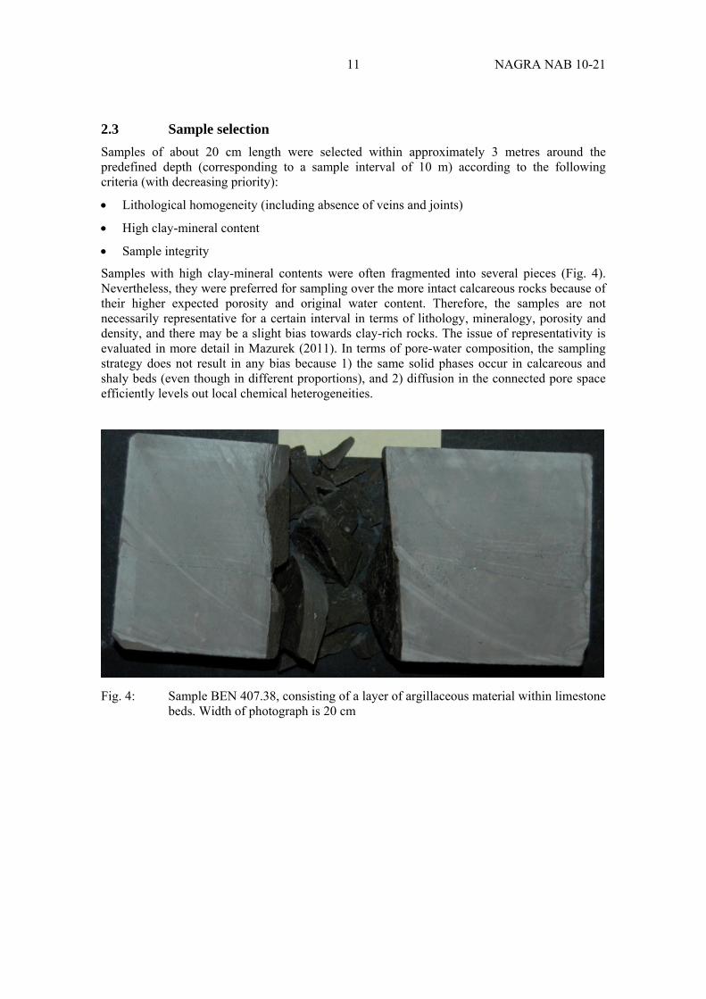
Samples with high clay-mineral contents were often fragmented into several pieces (Fig. 4). Nevertheless, they were preferred for sampling over the more intact calcareous rocks because of their higher expected porosity and original water content. Therefore, the samples are not necessarily representative for a certain interval in terms of lithology, mineralogy, porosity and density, and there may be a slight bias towards clay-rich rocks. The issue of representativity is evaluated in more detail in Mazurek (2011). In terms of pore-water composition, the sampling strategy does not result in any bias because 1) the same solid phases occur in calcareous and shaly beds (even though in different proportions), and 2) diffusion in the connected pore space efficiently levels out local chemical heterogeneities.

Fig. 4: Sample BEN 407.38, consisting of a layer of argillaceous material within limestone beds. Width of photograph is 20 cm

12 NAGRA NAB 10-21

3 Methods

3.1 Sample preparation

Samples were treated dry, and no cutting with a water-cooled diamond blade was involved. In cases when a sample was macroscopically homogeneous and there was plenty of material, only a part of the sample was crushed. In heterogeneous samples such as that shown in Fig. 4, only one type of material was selected. If possible, the more clay-rich part was selected, but in the majority of the cases there was not enough clay-rich material, and so the more calcareous part of the sample was processed.

After the separation of at least two representative subsamples for bulk dry density measurements, the 1 - 2 kg of sample material were crushed manually with hammer and chisel to pieces of about 1 cm size and then passed through a splitter. A split of about 300 g was ground in a tungsten carbide cup mill (100 g for about 30 s, resulting in a maximum grain size around 1 mm, and 200 g for about 2 min, yielding powders <63 µm).

3.2 Densities / Porosity

3.2.1 Bulk dry density

The bulk dry density b,dry was measured using the paraffin displacement method. The principle of the method is the calculation of bulk dry density from sample mass and volume making use of Archimedes' principle. Two separate and representative rock pieces with a volume of approximately 2-3 cm3 each were dried at 105 C. The sample volume was determined by weighing the rock sample in air and during immersion into paraffin oil (paraffin = 0.86 g/cm3 at 20 C) using a density accessory kit (Mettler Toledo). The bulk dry density was calculated according to:

b ,dry paraffin

mdry

mdry min paraffin

.

In data tables, the small-scale lithological heterogeneity is represented by the standard deviation of measurements on different subsamples. The analytical error of each individual measurement is dominated by the error on the density of the paraffin (0.86 ±0.01 g/cm3), which corresponds to an error on b,dry of ±1.2 %. Further sources of uncertainty include the representativity of the small rock pieces for the whole sample, the effects of drying (possible shrinkage of clay-rich samples) and of long-term storage (textural changes due to recurrent changes of temperature and air humidity, oxidation reactions; see Section 5.2 and Section 5.4).

3.2.2 Grain density

The grain density ρg was measured by kerosene pycnometry in duplicate. The volume of the pycnometer was derived from the weight of kerosene that filled the pycnometer without rock powder. The density of kerosene (ρk = 0.78 g/cm3 at 20 °C) was checked using an aerometer. After drying the powdered samples at 105 °C, approximately 15 g were placed in the pycnometer. The empty (mpycn) and the filled (mrock+pycn) flasks were weighed. The flask was subsequently filled with kerosene up to the meniscus while continuously removing the air by a vacuum pump and then weighed again (mrock+k+pycn). The grain density was obtained according to

13 NAGRA NAB 10-21

.

Some uncertainty mainly roots in the filling of the flask up to the meniscus. Care has to be taken when evacuating the flasks, in order to remove all air from the slurry (remaining air would lead to an underestimation of grain density). As for bulk dry density, the lithological heterogeneity on the sample scale is stated in data tables, represented by the standard deviation of measurements on different subsamples. The analytical uncertainty of each measurement is dominated by the error on the kerosene density (0.78 ±0.01 g/cm3) and yields an error for g of ±1.3 %.

3.2.3 Physical porosity

The physical porosity n is calculated from the bulk dry density and the grain density according to

For the uncertainty calculation, the Gaussian law of uncertainty propagation was applied. Let y be calculated from measured parameters x1, x2, ... with corresponding uncertainties u1, u2, ... . The uncertainty of y (uy) is then defined by

 

This means for the uncertainty in the particular case for the physical porosity:

In data tables, only the analytical errors on the density measurements were included in the calculation of the error on porosity, whereas lithological heterogeneity and other uncertainties, such as oxidation effects, were not considered at this stage.

3.3 Mineralogy

3.3.1 Whole-rock mineralogy by X-ray diffraction

For quantitative determination of the mineralogical composition, 3 g of each powdered sample were mixed with lithium fluoride (LiF) as an internal standard with a ratio of 10:1. Disoriented samples were measured on a Philips PW 1800 diffractometer using Cu Kα radiation. One X-ray pattern within the 2Θ range from 4° to 60° and one from 25° to 32° (duplicate) were recorded for each sample. In addition, a data acquisition program (GMP) that sweeps for a particular peak in a limited (±1°) 2Θ range and then measures the peak for 100 seconds was used on both duplicate samples. This, together with a measurement of either one or two background values at fixed 2Θ, allowed a more precise quantification than reading the counts from the regular X-ray pattern.

Calibration curves allowing an automatic quantification exist for quartz, calcite, dolomite, K-feldspar and plagioclase. Siderite was quantified by manually reading the intensity from the X-

14 NAGRA NAB 10-21

ray pattern and assuming the same concentration to intensity ratio as for the predominant carbonate (calcite or dolomite). However, the standardisation used for carbonates is only valid for individual mineral contents up to 50 %, which are exceeded in limestones. Therefore, the total inorganic carbon content determined by CS-Mat IR spectroscopy (see Section 3.3.3) was used to correct the carbonate contents. Pyrite content, which can only be qualitatively measured by XRD, was calculated from the S content obtained from the CS-Mat analysis, assuming that pyrite is the only S-containing phase. In cases where anhydrite was detected by XRD, all S was allocated to this phase, and no entry was made for pyrite.

When both anhydrite and dolomite were present (a common mineral assemblage in the Gipskeuper sequence), both peaks of the internal standard (LiF) interfere with the mineral peaks. To allow a quantitative measurement, another internal standard (such as fluorite; CaF2) could have been used. However, in this study, a Rietveld refinement method using structural data for LiF, anhydrite and dolomite was applied. This does not yield useful results directly because feldspars and phyllosilicates are difficult to refine due to their complex structure and chemical variability. Instead, the proportion of LiF contributing to the 38.6° peak (which is overlain by anhydrite) was estimated. This proportion has then been used to correct the regular GMP calculations. In cases where there was only little quartz and feldspar (the only minerals not corrected by CS-Mat), a semiquantitative RIR method was applied, as even major uncertainties would have a limited effect.

For every single sample, the X-ray pattern was assessed visually as well, in order to check for additional phases and to verify the results of the automatic calculations. The sum of sheet silicates, mainly clay minerals, was calculated by difference to 100 %.

3.3.2 Clay mineralogy by X-ray diffraction

To quantify the relative proportions of clay minerals, the <2µm fraction of the coarsely ground samples was separated by sedimentation in a 20 cm high Atterberg cylinder filled with a 0.01N NH4OH solution over 16 hours. The slurry was decarbonated using hydrochloric acid (HCl) and saturated with CaCl2, to replace the exchangeable cations by Ca. After pipetting the suspension on glass slides, one sample was dried under air, one was saturated with ethylene glycol (C2H6O2), and the third was heated for one hour at 550 °C. Ethylene glycol is used for the identification of expandable clay minerals, while the heating destroys kaolinite and allows a distinction from chlorite.

The three slides were scanned using a Philips PW 3710 diffractometer. Quantification of illite, chlorite, kaolinite and illite-smectite mixed layers was carried out visually by comparing peak intensities or areas.

3.3.3 CS-Mat IR spectroscopy

A rock powder (20 - 100 mg) was heated to 1350 - 1550 °C in an O2 or N2 atmosphere, and all volatile components were liberated at these temperatures. Total C and S were measured as CO2 and SO2 after oxidation in an O2 atmosphere. Inorganic C (i.e. essentially CO2 from carbonate minerals) was measured in a N2 atmosphere, assuming that the content of organic CO2 is negligible (this is mostly a reasonable assumption, but exceptions exist, e.g. some soils). The reaction gas was passed through a Mg perchlorate tube to remove water and then pumped through the CO2 and SO2 analysers. The peaks of CO2 and SO2 in the carrier gas were measured by IR spectroscopy. Separate NDIR analysers were used for each of the two species. Organic C was calculated by difference of total and inorganic C. Calibration was performed using pure CaCO3 for C and Ag2SO4 for S. Approximate detection limits are around 0.1 wt.-% for total C and S.

15 NAGRA NAB 10-21

3.4 Aqueous extraction

Aqueous extraction tests were performed at a solid:liquid (S:L) mass ratio of 1. The amount of pulped rock material was around 30 g. Each sample was prepared, extracted and analysed in duplicate under ambient conditions. Each suspension was shaken end-over-end for 24 hours in a polypropylene tube. After filtration using 0.45 µm millipore filters, the supernatant solutions were analysed for anions (F-, Cl-, SO4

--, NO3-) by ion chromatography, using a Metrohm 861

Compact IC-system. Br- and I- contents were obtained by ICP-MS at the British Geological Survey (BGS, Keyworth, UK).

16 NAGRA NAB 10-21

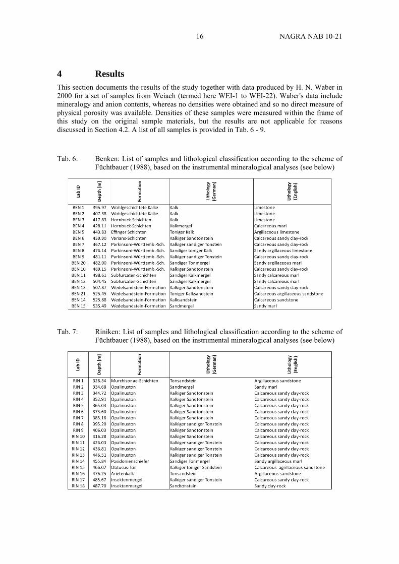
4 Results This section documents the results of the study together with data produced by H. N. Waber in 2000 for a set of samples from Weiach (termed here WEI-1 to WEI-22). Waber's data include mineralogy and anion contents, whereas no densities were obtained and so no direct measure of physical porosity was available. Densities of these samples were measured within the frame of this study on the original sample materials, but the results are not applicable for reasons discussed in Section 4.2. A list of all samples is provided in Tab. 6 - 9.

Tab. 6: Benken: List of samples and lithological classification according to the scheme of Füchtbauer (1988), based on the instrumental mineralogical analyses (see below)

Tab. 7: Riniken: List of samples and lithological classification according to the scheme of Füchtbauer (1988), based on the instrumental mineralogical analyses (see below)

17 NAGRA NAB 10-21

Tab. 8: Schafisheim: List of samples and lithological classification according to the scheme of Füchtbauer (1988), based on the instrumental mineralogical analyses (see below)

18 NAGRA NAB 10-21

Tab. 9: Weiach: List of samples and lithological classification according to the scheme of Füchtbauer (1988), based on the instrumental mineralogical analyses (see below)

19 NAGRA NAB 10-21

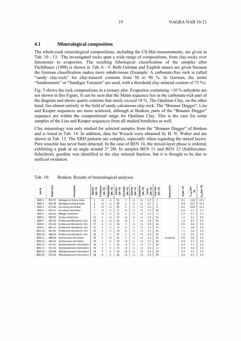
4.1 Mineralogical composition

The whole-rock mineralogical compositions, including the CS-Mat measurements, are given in Tab. 10 - 13. The investigated rocks span a wide range of compositions, from clay-rocks over limestones to evaporites. The resulting lithological classification of the samples after Füchtbauer (1988) is shown in Tab. 6 - 9. Both German and English names are given because the German classification makes more subdivisions (Example: A carbonate-free rock is called “sandy clay-rock” for clay-mineral contents from 50 to 90 %. In German, the terms “Sandtonstein” or “Sandiger Tonstein” are used, with a threshold clay-mineral content of 75 %).

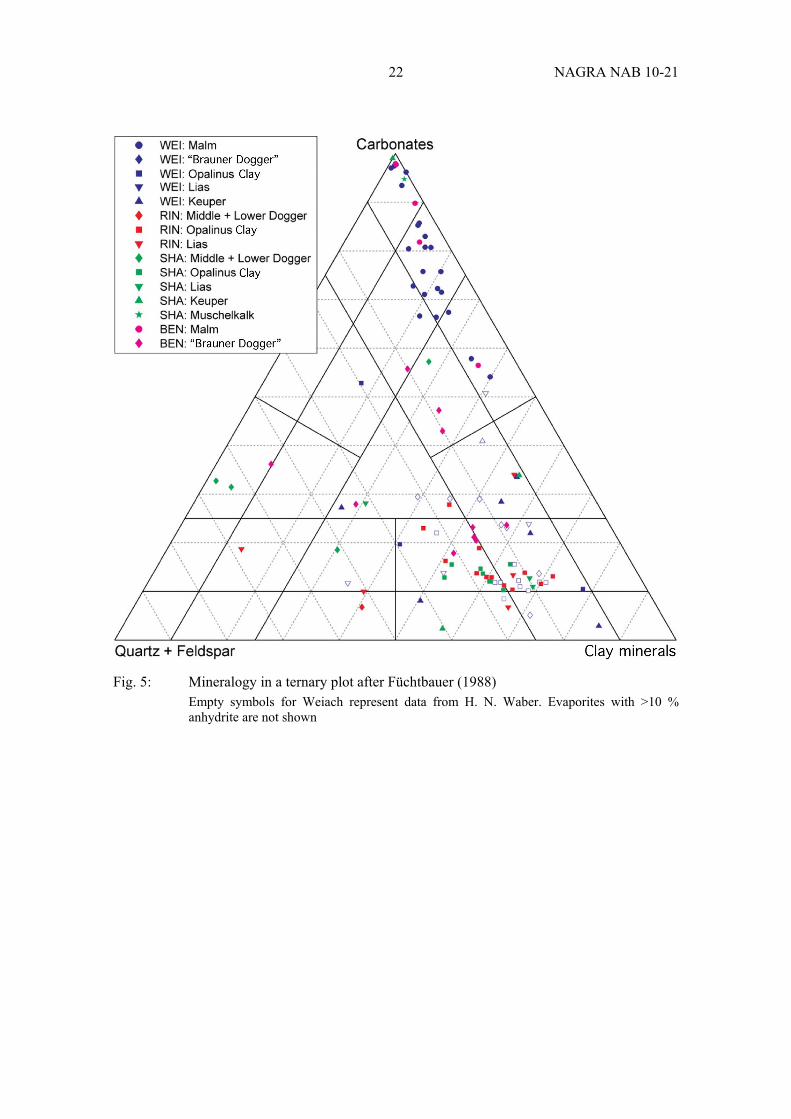
Fig. 5 shows the rock compositions in a ternary plot. Evaporites containing >10 % anhydrite are not shown in this Figure. It can be seen that the Malm sequence lies in the carbonate-rich part of the diagram and shows quartz contents that rarely exceed 10 %. The Opalinus Clay, on the other hand, lies almost entirely in the field of sandy calcareous clay-rock. The "Brauner Dogger", Lias and Keuper sequences are more scattered, although at Benken, parts of the "Brauner Dogger" sequence are within the compositional range for Opalinus Clay. This is the case for some samples of the Lias and Keuper sequences from all studied boreholes as well.

Clay mineralogy was only studied for selected samples from the "Brauner Dogger" of Benken and is listed in Tab. 14. In addition, data for Weiach were obtained by H. N. Waber and are shown in Tab. 15. The XRD patterns are complex, especially when regarding the mixed layers. Pure smectite has never been detected. In the case of BEN 14, the mixed-layer phase is ordered, exhibiting a peak at an angle around 3° 2Θ. In samples BEN 11 and BEN 12 (Subfurcaten-Schichten), goethite was identified in the clay mineral fraction, but it is thought to be due to surficial oxidation.

Tab. 10: Benken: Results of mineralogical analyses

20 NAGRA NAB 10-21

Tab. 11: Riniken: Results of mineralogical analyses

Tab. 12: Schafisheim: Results of mineralogical analyses

21 NAGRA NAB 10-21

Tab. 13: Weiach: Results of mineralogical analyses Data for samples WEI 1 to WEI 22 are from H. N. Waber

22 NAGRA NAB 10-21

Fig. 5: Mineralogy in a ternary plot after Füchtbauer (1988) Empty symbols for Weiach represent data from H. N. Waber. Evaporites with >10 % anhydrite are not shown

23 NAGRA NAB 10-21

Tab. 14: Benken: Results of analyses of clay mineralogy Data refer to weight fractions in the total rock. Ill./smec. ML: Illite-smectite mixed layers

Tab. 15: Weiach: Results of analyses of clay mineralogy Data of H. N. Waber. Data refer to weight fractions in the total rock. Ill./smec. ML: Illite-smectite mixed layers

24 NAGRA NAB 10-21

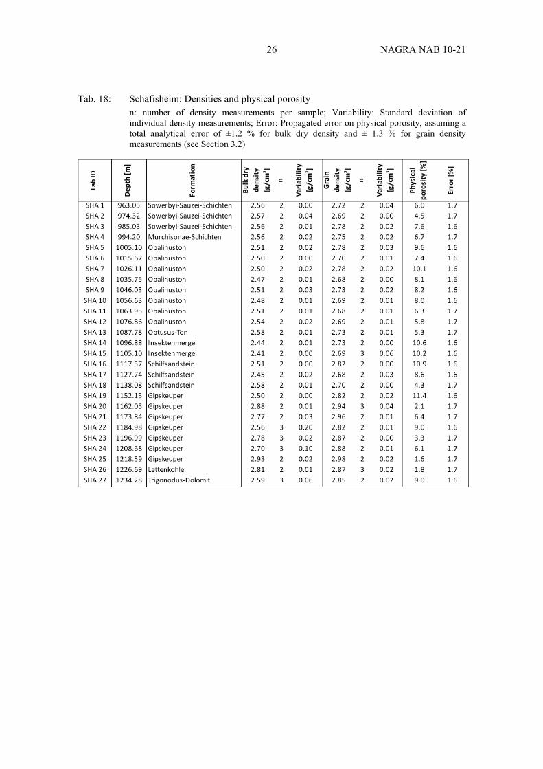
4.2 Densities and physical porosity

The measured bulk dry and grain densities and calculated physical porosities are listed in Tab. 16 - 19. Routinely, two measurements (on different rock materials) of bulk dry and grain densities were performed per sample, and the average is listed and used for further calculations. If the standard deviation between these measurements exceeded 0.04 g/cm3, another measurement was made. Some samples still show a high variability (e.g. in the Gipskeuper of Schafisheim and Weiach). This scatter reflects the lithological heterogeneity on the scale of the sample size and not analytical problems. Note that the error on physical porosity listed in Tab. 16 - 19 relates exclusively to the analytical uncertainty on the density measurements and is around 1.6 % irrespective of the porosity value. In low-porosity rocks (<5 %), the relative error on porosity calculated from densities becomes large, and the data need to be interpreted with care. The additional uncertainty related to sample heterogeneity is taken into account in the data-screening procedure (Section 6.2).

A set of samples from Weiach was studied previously by H. N. Waber. Since then, the sample materials have been stored at room temperature in the Institute of Geological Sciences at Bern over several years. These materials were used again in this study for the density measurements. However, the samples showed extensive oxidation phenomena and were crumbly, in particular the clay-rich lithiologies. Some of the porosities calculated from the data were aberrantly high. It appears that the long-term storage of unprotected samples under indoor conditions led to a stronger deterioration when compared to samples taken from intact core materials sealed into plastic sleeves. Therefore, the new density data produced on Waber's samples are not considered trustworthy and were eliminated from the data base.

Tab. 16: Benken: Densities and physical porosity n: number of density measurements per sample; Variability: Standard deviation of individual density measurements; Error: Propagated error on physical porosity, assuming a total analytical error of ±1.2 % for bulk dry density and ± 1.3 % for grain density measurements (see Section 3.2)

25 NAGRA NAB 10-21

Tab. 17: Riniken: Densities and physical porosity n: number of density measurements per sample; Variability: Standard deviation of individual density measurements; Error: Propagated error on physical porosity, assuming a total analytical error of ±1.2 % for bulk dry density and ± 1.3 % for grain density measurements (see Section 3.2)

26 NAGRA NAB 10-21

Tab. 18: Schafisheim: Densities and physical porosity n: number of density measurements per sample; Variability: Standard deviation of individual density measurements; Error: Propagated error on physical porosity, assuming a total analytical error of ±1.2 % for bulk dry density and ± 1.3 % for grain density measurements (see Section 3.2)

27 NAGRA NAB 10-21

Tab. 19: Weiach: Densities and physical porosity n: number of density measurements per sample; Variability: Standard deviation of individual density measurements; Error: Propagated error on physical porosity, assuming a total analytical error of ±1.2 % for bulk dry density and ± 1.3 % for grain density measurements (see Section 3.2)

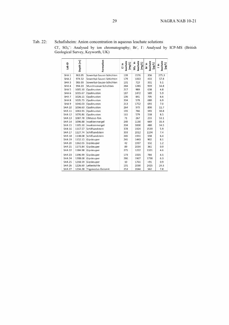
4.3 Anion concentrations

Anion concentrations obtained from aqueous extractions are reported in Tab. 20 - 23. All data are given in units of mass per Lsolution, which, at the chosen solid:liquid mass ratio of 1, corresponds to mass per kgrock. Reported values are averages of duplicate measurements.

Measured SO42- concentrations are high but most probably not representative of in-situ pore

water. Given the long-term storage of the samples under atmospheric conditions and the fact that the extractions were prepared under ambient laboratory conditions, SO4

2- is strongly affected by pyrite oxidation. In anhydrite-bearing samples (mainly Gipskeuper), anhydrite

28 NAGRA NAB 10-21

dissolution is another source of SO42-. I- contents in pore waters of marine sedimentary rocks are

typically much higher than in sea water because the main contribution originates from the decomposition of organic matter during diagenesis (see also Mazurek et al. 2011). Thus, because I- is not strictly conservative and depends on the nature and concentration of organic matter, it is not considered here any further. Therefore, further use of anion concentrations is limited to chloride ±bromide.

Tab. 20: Benken: Anion concentration in aqueous leachate solutions Cl-, SO4

--: Analysed by ion chromatography; Br-, I-: Analysed by ICP-MS (British Geological Survey, Keyworth, UK)

Tab. 21: Riniken: Anion concentration in aqueous leachate solutions Cl-, SO4

--: Analysed by ion chromatography; Br-, I-: Analysed by ICP-MS (British Geological Survey, Keyworth, UK)

29 NAGRA NAB 10-21

Tab. 22: Schafisheim: Anion concentration in aqueous leachate solutions Cl-, SO4

--: Analysed by ion chromatography; Br-, I-: Analysed by ICP-MS (British Geological Survey, Keyworth, UK)

30 NAGRA NAB 10-21

Tab. 23: Weiach: Anion concentration in aqueous leachate solutions Data for samples WEI 1 to WEI 22 are from H. N. Waber. Cl-, SO4

--: Analysed by ion chromatography; Br-, I-: Analysed by ICP-MS (British Geological Survey, Keyworth, UK)

31 NAGRA NAB 10-21

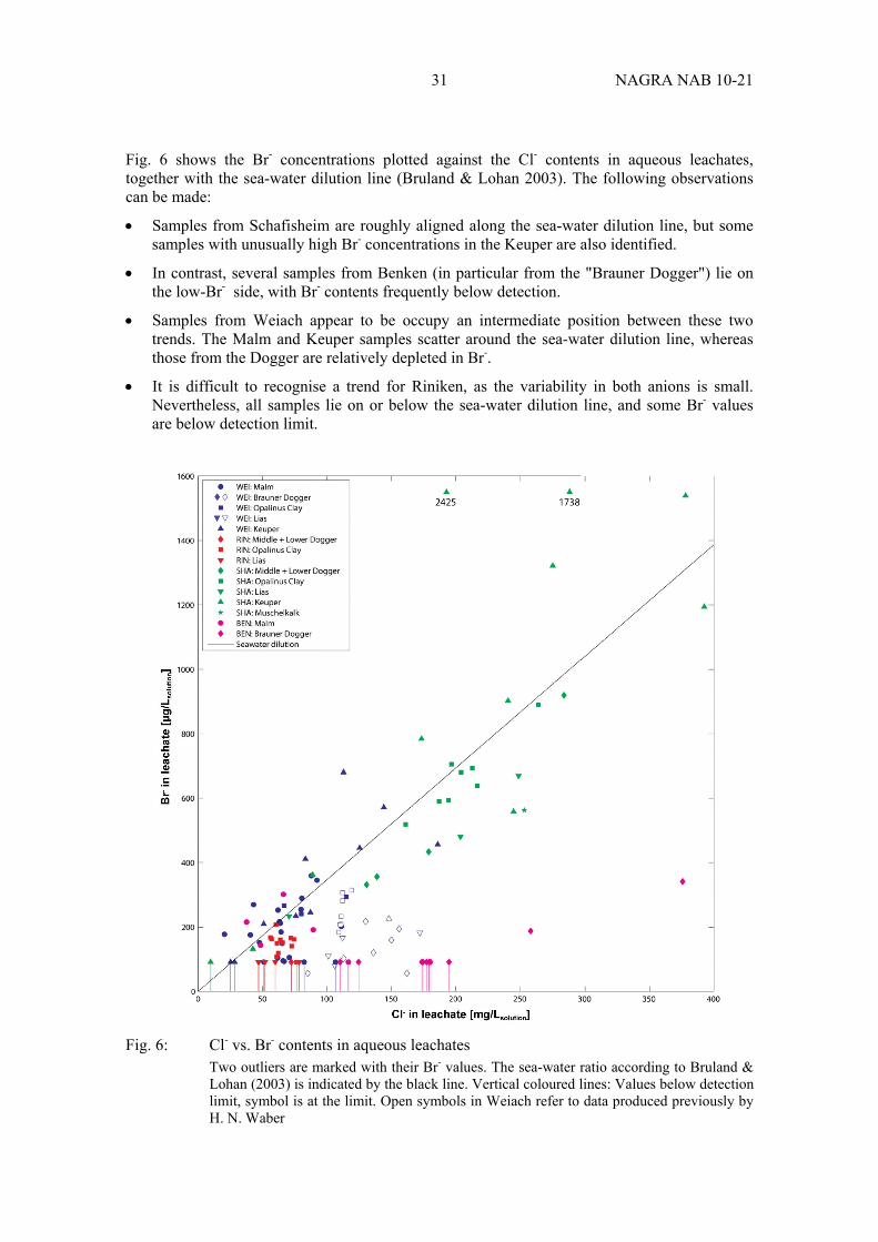
Fig. 6 shows the Br- concentrations plotted against the Cl- contents in aqueous leachates, together with the sea-water dilution line (Bruland & Lohan 2003). The following observations can be made:

Samples from Schafisheim are roughly aligned along the sea-water dilution line, but some samples with unusually high Br- concentrations in the Keuper are also identified.

In contrast, several samples from Benken (in particular from the "Brauner Dogger") lie on the low-Br- side, with Br- contents frequently below detection.

Samples from Weiach appear to be occupy an intermediate position between these two trends. The Malm and Keuper samples scatter around the sea-water dilution line, whereas those from the Dogger are relatively depleted in Br-.

It is difficult to recognise a trend for Riniken, as the variability in both anions is small. Nevertheless, all samples lie on or below the sea-water dilution line, and some Br- values are below detection limit.

Fig. 6: Cl- vs. Br- contents in aqueous leachates Two outliers are marked with their Br- values. The sea-water ratio according to Bruland & Lohan (2003) is indicated by the black line. Vertical coloured lines: Values below detection limit, symbol is at the limit. Open symbols in Weiach refer to data produced previously by H. N. Waber

32 NAGRA NAB 10-21

5 Derivation of pore-water concentrations of anions: Analysis of methodological approaches based on data from the Benken borehole

5.1 Formalism

The conversion of the aqueous-leaching data from concentrations per L of leach solution to pore-water concentrations is performed according to

Cpwmg

Lpore water

CAqExmg

Lsolution

L Lsolution S kgdry rock

g

kgdry rock

Lrock

(1 n)

n

with Cpw = concentration of solute in pore water CAqEx = concentration of solute in aqueous extract L/S = liquid/solid ratio in aqueous-leaching experiments g = grain density n = physical porosity = fraction of physical porosity accessible to the solute.

This equation requires knowledge of both physical and of anion-accessible porosity. Given the fact that the samples studied here are at least 10 years old, the determination of porosities is more uncertain than in the situation when the samples are fresh and saturated.

5.2 Methods to constrain physical porosity

Physical porosity for the Benken samples was estimated by three independent methods. These, together with their inherent uncertainties, are listed in Tab. 24.

33 NAGRA NAB 10-21

Tab. 24: Methods to constrain physical porosity in the present study

Method Uncertainties

1. Porosity calculated from measured bulk dry and grain densities

Possibly limited representativity of measured densities (in particular bulk dry density) for the original in-situ conditions: • Samples were exposed to variable temperature and air humidity

over many years, with possible effects on pore structure • Oxidation reactions, e.g. the conversion of pyrite to gypsum

2. Porosity calculated from RHOB density borehole log

• Vertical resolution of the log is in the range of several dm and so not necessarily sample-specific (average sample length is 22 cm)

• Quality of RHOB log strongly depends on borehole quality; no data (or interpolated data) are available in zones with breakouts; logs need to be edited using the caliper log. Breakouts lower RHOB density and so yield an overestimation of porosity

• The calculation of porosity requires knowledge of grain density, which has to be constrained by other methods (laboratory measurements on cores or calculation based on mineralogical composition using generic mineral densities)

3. Porosity calculated from clay-mineral content

In clay-carbonate mixtures, a site- or region-specific correlation may be defined. In this study, the following constraints apply: • The number of data that can be used for the correlation is limited,

even if the whole Jurassic sequence is considered (the Triassic is excluded because of the occurrence of a wider lithological spectrum (sandstones, evaporites))

• The correlation is not well defined, correlation factors are low • Porosity depends not only on clay-mineral content but also on

maximum burial depth, which varies over the region

5. 3 Approaches to defining the anion-accessible porosity fraction

In Opalinus Clay, about half of the physical porosity is accessible to anions (Gimmi & Waber 2004, Pearson et al. 2003, Koroleva et al. 2011). However, the low-permeability sequence is lithologically heterogeneous, so it is questionable whether the value for Opalinus Clay is representative of the whole profile. The following alternatives were chosen and are illustrated in Fig. 7:

1. The whole physical porosity was assumed to be anion-accessible, i.e. all solute concentrations in leachates were directly related to physical porosity;

2. In line with Gimmi & Waber (2004), the anion-accessible porosity fraction was chosen as 0.5 for the whole sequences, irrespective of mineralogy. A cutoff was selected at 10 % clay-mineral content (limestones), at and below which the whole physical porosity was considered to be anion-accessible;

3. A hypothetic function was chosen that considers an anion-accessible porosity fraction of 0.5 in claystones (≥60 % clay-mineral content) and a linear increase towards 1 with decreasing clay-mineral content.

34 NAGRA NAB 10-21

Fig. 7: Hypotheses relating the anion-accessible porosity fraction to clay-mineral content

5.4 Analysis of methods to derive physical and anion-accessible porosity

The approaches presented in Sections 5.2 and 5.3 are explored here using the information from the Benken borehole. This choice was made because abundant data are available from this site (mineralogy, porosity: Nagra 2001, Waber et al. 2003, this study; anion contents: Waber et al. 2003, this study).

5.4.1 Porosity calculated from measured bulk dry and grain densities and from gravimetric water loss

Porosity data calculated from density measurements and from gravimetric water loss of saturated samples are known to yield comparable results (see, e.g., Nagra 2002), and so are treated together here. Three data sets are available (Tab. 25, Fig. 8):

1. Densities and calculated physical porosity based on this study, i.e. performed on 10 years old materials (focussed on samples from the "Brauner Dogger", see also Tab. 16). Uncertainties related to the age of the samples are listed in Tab. 24.

2. Water-loss porosity data from Waber et al. (2003) obtained from gravimetric water contents of freshly drilled core material.

3. Densities and calculated physical porosity based on Nagra (2001). The data were produced shortly after drilling and so are not affected by artefacts due to long-term storage. On the other hand, they were obtained by different methods than those for this study.

35 NAGRA NAB 10-21

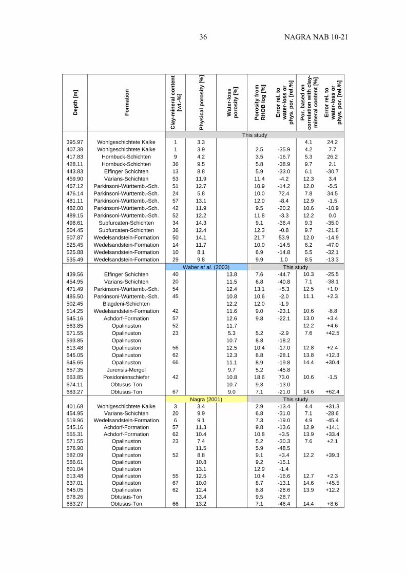
Tab. 25: Comparison of porosities of Benken drillcores (Jurassic section) derived from different methods Upper part: Physical porosity obtained from density measurements in this study, i.e. based on 10 years old core materials, compared with alternative methods to constrain porosity. Central part: Porosity obtained from water-loss measurements of the freshly drilled core (Waber et al. 2003), compared with alternative methods to constrain porosity. Bottom part: Physical porosity obtained from density measurements by Nagra (2001), based on fresh core materials, compared with alternative methods to constrain porosity. One low-porosity sample from the Jurensis-Mergel is excluded from the comparison because of the large analytical error

36 NAGRA NAB 10-21

D

epth

[m] 

Form

atio

n 

Cla

y-m

iner

al c

onte

nt

[wt.-

%] 

Phys

ical

por

osity

[%] 

Wat

er-lo

ss

poro

sity

[%] 

Poro

sity

from

R

HO

B lo

g [%

] 

Erro

r rel

. to

w

ater

-loss

or

phys

. por

. [re

l.%]

Por.

base

d on

co

rrel

atio

n w

ith c

lay-

min

eral

con

tent

[%] 

Erro

r rel

. to

w

ater

-loss

or

phys

. por

. [re

l.%]

This study 395.97 Wohlgeschichtete Kalke 1 3.3   4.1 24.2 407.38 Wohlgeschichtete Kalke 1 3.9   2.5 -35.9 4.2 7.7 417.83 Hornbuck-Schichten 9 4.2   3.5 -16.7 5.3 26.2 428.11 Hornbuck-Schichten 36 9.5   5.8 -38.9 9.7 2.1 443.83 Effinger Schichten 13 8.8   5.9 -33.0 6.1 -30.7 459.90 Varians-Schichten 53 11.9   11.4 -4.2 12.3 3.4 467.12 Parkinsoni-Württemb.-Sch. 51 12.7   10.9 -14.2 12.0 -5.5 476.14 Parkinsoni-Württemb.-Sch. 24 5.8   10.0 72.4 7.8 34.5 481.11 Parkinsoni-Württemb.-Sch. 57 13.1   12.0 -8.4 12.9 -1.5 482.00 Parkinsoni-Württemb.-Sch. 42 11.9   9.5 -20.2 10.6 -10.9 489.15 Parkinsoni-Württemb.-Sch. 52 12.2   11.8 -3.3 12.2 0.0 498.61 Subfurcaten-Schichten 34 14.3   9.1 -36.4 9.3 -35.0 504.45 Subfurcaten-Schichten 36 12.4   12.3 -0.8 9.7 -21.8 507.87 Wedelsandstein-Formation 50 14.1   21.7 53.9 12.0 -14.9 525.45 Wedelsandstein-Formation 14 11.7   10.0 -14.5 6.2 -47.0 525.88 Wedelsandstein-Formation 10 8.1   6.9 -14.8 5.5 -32.1 535.49 Wedelsandstein-Formation 29 9.8   9.9 1.0 8.5 -13.3

Waber et al. (2003) This study 439.56  Effinger Schichten  40   13.8  7.6  -44.7  10.3 -25.5 454.95  Varians-Schichten  20   11.5  6.8  -40.8  7.1 -38.1 471.49  Parkinsoni-Württemb.-Sch.  54   12.4  13.1  +5.3  12.5 +1.0 485.50  Parkinsoni-Württemb.-Sch.  45   10.8  10.6  -2.0  11.1 +2.3 502.45  Blagdeni-Schichten    12.2  12.0  -1.9 

514.25  Wedelsandstein-Formation  42   11.6  9.0  -23.1  10.6 -8.8 545.16  Achdorf-Formation  57   12.6  9.8  -22.1  13.0 +3.4 563.85  Opalinuston  52   11.7      12.2 +4.6 571.55  Opalinuston  23   5.3  5.2  -2.9  7.6 +42.5 593.85  Opalinuston    10.7  8.8  -18.2 

613.48  Opalinuston  56   12.5  10.4  -17.0  12.8 +2.4 645.05  Opalinuston  62   12.3  8.8  -28.1  13.8 +12.3 645.65  Opalinuston  66   11.1  8.9  -19.8  14.4 +30.4 657.35  Jurensis-Mergel    9.7  5.2  -45.8 

663.85  Posidonienschiefer  42   10.8  18.6  73.0  10.6 -1.5 674.11  Obtusus-Ton    10.7  9.3  -13.0 

683.27  Obtusus-Ton  67   9.0  7.1  -21.0  14.6 +62.4

Nagra (2001) This study 401.68 Wohlgeschichtete Kalke 3 3.4 2.9 -13.4 4.4 +31.3 454.95 Varians-Schichten 20 9.9 6.8 -31.0 7.1 -28.6 519.96 Wedelsandstein-Formation 6 9.1 7.3 -19.0 4.9 -45.4 545.16 Achdorf-Formation 57 11.3 9.8 -13.6 12.9 +14.1 555.31 Achdorf-Formation 62 10.4 10.8 +3.5 13.9 +33.4 571.55 Opalinuston 23 7.4 5.2 -30.3 7.6 +2.1 576.90 Opalinuston 11.5 5.9 -48.5 582.09 Opalinuston 52 8.8 9.1 +3.4 12.2 +39.3 586.61 Opalinuston 10.8 9.2 -15.1 601.04 Opalinuston 13.1 12.9 -1.4 613.48 Opalinuston 55 12.5 10.4 -16.6 12.7 +2.3 637.01 Opalinuston 67 10.0 8.7 -13.1 14.6 +45.5 645.05 Opalinuston 62 12.4 8.8 -28.6 13.9 +12.2 678.26 Obtusus-Ton 13.4 9.5 -28.7 683.27 Obtusus-Ton 66 13.2 7.1 -46.4 14.4 +8.6

37 NAGRA NAB 10-21

Physical porosity based on this study Water-loss porosity based on

Waber et al. (2003) Physical porosity based on Nagra (2001)

Fig. 8: Comparison of porosities of Benken drillcores (Jurassic section) derived from different methods (based on data from Tab. 25) Black lines indicate 1:1 correlations. Left: Physical porosity obtained from density measurements in this study, i.e. based on 10 years old core materials, compared with alternative methods to constrain porosity. Centre: Porosity obtained from water-loss measurements of the freshly drilled core (Waber et al. 2003), compared with alternative methods to constrain porosity. Right: Physical porosity obtained from density measurements by Nagra (2001), based on fresh core materials, compared with alternative methods to constrain porosity. One low-porosity sample from the Jurensis-Mergel is excluded from the comparison because of the large analytical error

38 NAGRA NAB 10-21

5.4.2 Porosity calculated from RHOB density log

A quality-assured RHOB log (RHOB) for the Benken borehole is available in Nagra (2001). The grain densities were derived from mineral-specific values (calcite: 2.71 g/cm3, dolomite: 2.845 g/cm3, clay minerals: 2.64 g/cm3, quartz: 2.625 g/cm3, anhydrite: 2.97 g/cm3, pyrite: 5.01 g/cm3) and from the mineralogical log from Nagra (2001), which provides a continuous depth profile for the contents of clay minerals, carbonates, anhydrite and quartz. In the Jurassic section, carbonate was assumed to be pure calcite, and all samples were assumed to contain 0.5 wt.-% pyrite. In the Triassic, a dolomite/calcite ratio of 3 was used, and no pyrite was considered. Porosity was calculated according to

n g RHOB

g fluid

,

with fluid = fluid density = 1 g/cm3. The resulting data are listed in Tab. 25.

5.4.3 Porosity calculated from clay-mineral content

In order to establish an empirical relationship between clay-mineral content and physical porosity, only Jurassic samples from this study were used. Jurassic lithologies can be roughly conceived as mixtures of clay minerals and calcite in variable proportions, whereas the lithological spectrum is more complex in the Triassic (including sandstones, evaporites, dolomitic rocks). In addition to data from Benken, those from Weiach were also included in the analysis, in order to augment the data base. This is justified because the burial histories of Benken and Weiach are similar, whereas those of the other studied boreholes are different (Mazurek et al. 2006) and so may lead to different porosities at a given clay-mineral content. The resulting correlation is shown in Fig. 9a. The regression is not overly well defined, the scatter of the data is considerable. Porosities derived from the regression of clay-mineral contents (black line in Fig. 9a) are given in Tab. 25.

Further data on clay-mineral contents and porosities from Benken and Weiach are available from the original reports prepared in the context of the respective drilling campaigns (Nagra 2001, Matter et al. 1988a; data compiled in Mazurek 2011). The advantage of these data is the fact that the analyses were made shortly after core recovery, so effects of oxidation and long-term storage are expected to be less important. However, the data, as illustrated in Fig. 9b, show a more substantial scatter than those obtained in the frame of this study (Fig. 9a), and a meaningful regression of porosities to clay-mineral contents cannot be obtained. The reasons for the scatter are not entirely clear. It must be noted that the methodology used to measure densities that underlie the porosities of Fig. 9b was different from that used here.

39 NAGRA NAB 10-21

a. b.

Fig. 9: Correlation of clay-mineral contents and porosities of the Jurassic sections in boreholes Benken and Weiach a. Data from this study

b. Data from Nagra (2001) and Matter et al. (1988a)

5.4.4 Evaluation of methods to constrain porosity

Because the true porosity values are not known and each method has its own uncertainties (see Tab. 24), it is not possible to evaluate the adequacy of the individual data sets against an accepted benchmark. Porosities estimated from the RHOB log and from clay-mineral content show deviations from physical or water-loss porosity of up to 73 % relative. The average relative errors are ±20 - 25 % for both RHOB-derived porosities and for porosities estimated from clay-mineral contents (Tab. 25).

Because a clearly preferred method to characterise porosity of "historic" samples has not been identified, they were all considered here in alternative cases for the derivation of pore-water concentrations of solutes according to the equation given in Section 5.1. Together with the 3 alternative ways to take into account anion exclusion (Section 5.3, Fig. 7), a total of 9 cases were explored. The resulting pore-water concentrations of Cl- are listed in Tab. 26 and plotted in Fig. 10 - 12.

Given the fact that the pore-water profile in Benken is considered to be dominated by diffusion (Gimmi & Waber 2004, Gimmi et al. 2007), a regular pattern of the spatial Cl- distribution would be expected. Therefore, recalculation methods that yield regular patterns are considered as more appropriate, whereas scattered distributions are thought to be more strongly affected by artefacts or inadequate assumptions. In this respect, inspection of Fig. 10 - 12 leads to the following insights:

• In Fig. 10, the data of Waber et al. (2003) (shown in blue) yield a regular pattern when using the original water-loss porosities for the recalculation (left). An almost equally regular pattern is obtained when using porosities derived from the correlation with clay-mineral contents (right). In contrast, the pattern obtained when using porosities derived from the RHOB log is scattered and probably not representative.

40 NAGRA NAB 10-21

• In the same Figure, the data produced in this study (red) are substantially more strongly scattered than those of Waber et al. (2003), which reflects the larger uncertainties regarding porosity. Remarkably, the distribution is most regular when using porosities derived from clay-mineral contents (right), even though 3 points fall off the general trend (for a discussion of these data, see screening of the results in Section 6.2). In any case, this data set appears to be better interpretable than the other two.

• Fig. 11, in which the same data are shown but where, in addition, a scaling for the anion-accessible porosity fraction was applied (factor 0.5 for samples with clay-mineral contents >10 wt.-%), yields similar conclusions. The central graph based on RHOB data is quite scattered, whereas the other two show clearer trends (in spite of some outliers in the data set produced in this study). The Cl- concentration in the shallowest sample is reasonably close to that of the overlying Malm aquifer (4356 mg/L at a depth of 380 - 394.8 m; see Tab. 2).

• In the graphs shown in Fig. 12, anion exclusion is considered using a scaling factor that depends on clay-mineral content (Section 5.3). In comparison to the alternatives shown in the previous Figures, the scatter of the data is clearly higher, in particular in those of Waber et al. (2003). It appears that a constant scaling factor (except in limestones) better approaches the in-situ values.

5.5 Conclusions for the calculation of pore-water concentrations of solutes

Based on the analysis in the previous Section, the following conclusions are made:

• Aqueous-leaching data are ideally recalculated using water-loss porosity of the same samples. In the absence of water-loss porosity data, the second choice is porosity derived by correlation to clay-mineral content. Porosity based on new density measurements on the 10 years old samples is the third choice. Porosity derived from the RHOB log cannot be used, probably due to the more limited spatial resolution of this method and because of possible artefacts, e.g. breakouts).

• Regarding the scaling factor that considers anion exclusion in clay-bearing rocks, the variant using a constant factor in conjunction with a cutoff at 10 % clay-mineral content yields more consistent results than a mineralogy-dependent function. It will be used for the calculations in Section 6 below. In the absence of direct experimental data, it is difficult to provide an error estimation for this approach.

41 NAGRA NAB 10-21

Tab. 26: Pore-water chloride contents calculated from aqueous-leaching data of Benken samples using a set of alternative assumptions regarding porosity The same procedures were applied to the original leaching data (concentrations per L leach solution) from this study and to those from Waber et al. (2003)

42 NAGRA NAB 10-21

Fig. 10: Chloride contents from aqueous leaching of Benken samples recalculated to pore-water contents without any correction for the anion-accessible porosity fraction Red: leaching data from this study; blue: leaching data from Waber et al. (2003). Left: Recalculation based on physical porosity obtained from density measurements (data from this study) or water-loss porosity (data from Waber et al. 2003). Centre: Recalculation based on porosity obtained from RHOB borehole log. Right: Recalculation based on porosity derived from the correlation with clay-mineral contents

43 NAGRA NAB 10-21

Fig. 11: Chloride contents from aqueous leaching of Benken samples recalculated to pore-water contents, considering a scaling factor of 0.5 for the anion-accessible porosity fraction in samples with >10 wt.-% clay-mineral content Red: leaching data from this study; blue: leaching data from Waber et al. (2003). Left: Recalculation based on physical porosity obtained from density measurements (data from this study) or water-loss porosity (data from Waber et al. 2003). Centre: Recalculation based on porosity obtained from RHOB borehole log. Right: Recalculation based on porosity derived from the correlation with clay-mineral contents

44 NAGRA NAB 10-21

Fig. 12: Chloride contents from aqueous leaching of Benken samples recalculated to pore-water contents, considering a mineralogy-dependent scaling factor for the anion-accessible porosity fraction (see text) Red: leaching data from this study; blue: leaching data from Waber et al. (2003). Left: Recalculation based on physical porosity obtained from density measurements (data from this study) or water-loss porosity (data from Waber et al. 2003). Centre: Recalculation based on porosity obtained from RHOB borehole log. Right: Recalculation based on porosity derived from the correlation with clay-mineral contents

45 NAGRA NAB 10-21

6 Calculated pore-water concentrations of Cl- in all boreholes

6.1 Analysis of errors and error propagation

Pore-water concentrations of solutes are recalculated from concentrations in aqueous extracts (CAqEx) to pore-water concentrations (Cpw) using the equation given in Section 5.1. Apart from CAqEx, the parameters in this equation include grain density (g), porosity (n) (and therefore bulk dry density b,dry that is used to calculate porosity) and the anion-accessible porosity fraction (). All these parameters are subject to errors and uncertainties, and Tab. 27 provides an overview of these. The total error is dominated by uncertainties regarding porosity and the fraction that is accessible to anions.

6.1.1 Porosity obtained from density measurements

The purely analytical errors on the measurement of bulk dry and grain density are about ±1.2 and 1.3 %rel., originating mainly from the error on the density of the immersion fluid (paraffin, kerosene) that is used to calculate the rock density values. These errors correspond to absolute errors of about 0.03 - 0.035 g/cm3 for both densities. Using the error-propagation function formulated in Section 3.2.3, these errors propagate into an error of around ±1.6 vol.-% on porosity. This error remains essentially constant irrespective of the porosity value. Therefore, the relative error increases with decreasing porosity.

The long-term storage of the core materials under atmospheric conditions is a further potential source of uncertainty that adds up with the analytical error. In order to capture this effect, an additional estimated error of 20 % rel. was applied on porosity. For a rock with a porosity of 10 %, the total uncertainty of 3.6 vol.-% (considering both the analytical and the sample storage uncertainties) corresponds to a relative error of ±36 %rel.. For a rock with a porosity of 5 %, the relative error becomes ±52 %rel..

6.1.2 Porosity obtained by regression to clay-mineral content

A linear correlation was established between clay-mineral content and physical porosity for Jurassic samples from the Benken and Weiach boreholes analysed in this study (Section 5.4.3, Fig. 9a). Porosity values calculated from known clay-mineral contents were then compared with porosities derived from water-loss and density measurements on fresh samples from Benken (Tab. 25). This comparison indicated that 68 % of the calculated porosities are within ±30 %rel. of the values based on density and water-loss measurement. Therefore, an estimated error of ±30 %rel. is propagated into the calculation of solute concentrations in pore water.

The regression line obtained for samples from Benken and Weiach is also used below for the other boreholes. This adds another element of uncertainty because the burial histories of these boreholes differ somewhat from that of the Benken/Weiach region (Mazurek et al. 2006). In principle, the relationship between clay-mineral content and porosity should be elaborated for each borehole, but this is not feasible in this case due to the limited data available from boreholes Riniken and Schafisheim.

46 NAGRA NAB 10-21

Tab. 27: Definition and quantification of errors of parameters that are used to calculate pore-water concentrations of solutes

Parameter Symbol Source of error Quantification of error

Further sources of error not included in the

quantification Solute

concentration in aqueous extract

CAqEx Analytical error of IC or

ICP-MS analysis ±5 %rel. for Cl-,

±15 %rel. for Br- and I-

Grain density rg

Analytical error, dominated by the error on kerosene density (±0.01

g/cm3)

±1.3 % rel. Sample heterogeneity

Bulk dry density rb,dry

Analytical error, dominated by the error on

paraffin density (±0.01 g/cm3)

±1.2 % rel.

• Sample heterogeneity • Textural and

mineralogical changes due to long-term storage of core materials under atmospheric conditions

• Possible shrinkage of clay-rich samples due to drying (for a discussion of this effect see Mazurek et al. 2010)

Analytical error on density measurements

Calculated from errors on rb,dry and rg:

yields ca. ±1.6 vol.-%, independently of the

value of porosity Physical porosity

(obtained from density

measurements)

n Effects of textural and mineralogical changes

due to long-term storage of core materials under atmospheric conditions

on rb,dry

±20 % rel. of the porosity value

(estimate)

• Sample heterogeneity • Possible shrinkage of

clay-rich samples due to drying (for a discussion of this effect see Mazurek et al. 2010)

Porosity obtained by

regression to clay-mineral

content

n Definition of the regression line

±30 %rel. (based on comparison with

porosities obtained from water-loss and

density measurements, see Tab. 25)

Extrapolation of the regression developed for

Benken and Weiach to the other boreholes

Anion-accessible

porosity fraction a

Conceptual assumption on the fraction of physical

porosity accessible to anions

Not quantified

6.1.3 Calculation of total errors

The propagated error on the calculated concentrations is quantified using the Gaussian law of uncertainty propagation applied to the equation given in Section 5.1. The rock/water ratio L/S [Lsolution/kgdry rock] of the experiments was 1, so this term drops out from the equation. The partial derivatives that propagate the errors (u) on the concentration in the extract (CAqEx), grain density (g) and porosity (n) are

47 NAGRA NAB 10-21

,

leading to a total uncertainty on the pore-water concentration of

.

Note that the error on the fraction of porosity that is accessible to anions (, see Section 5.3) cannot be quantified because it relies on conceptual assumptions that cannot currently be rigorously tested against experimental data.

6.2 Calculated Cl- concentrations in pore water and data screening

The resulting pore-water concentrations of Cl-, including the propagated errors according to Tab. 27, are listed in Tab. 28 - 31 for boreholes Benken, Riniken, Schafisheim and Weiach. Results are shown both for concentrations recalculated using physical porosity based on density measurements in this study and for those recalculated using the regression to clay-mineral contents. The anion-accessible porosity fraction was assumed to be 0.5 for rocks with >10 wt.-% clay-mineral content and 1 for ≤10 wt.-% clay-mineral content. Graphical representations of the results are shown in Fig. 13 - 20.

The spatial distributions of Cl- do show depth trends. Interestingly, clearer and more consistent depth profiles are obtained when the recalculation of the concentrations is based on porosities obtained from the regression to clay-mineral contents. Nevertheless, there are a number of outliers that do not fit the patterns, and an attempt was made to explain these:

• Some of the outliers are likely due to the somewhat artificial choice of the limit at 10 wt.-% clay-mineral content at and below which the anion-accessible porosity fraction is assumed to be 1 (see e.g. 4 samples between 300 and 400 m in Weiach, Fig. 20).

• A source of error that is not considered by the error bars is sample heterogeneity on the scale of centimetres. Homogeneity was one of the first-order criteria to select core samples for this study. Nevertheless, marked heterogeneity was identified in some samples, in particular in the Keuper. If the sample materials on which porosity, mineralogy and Cl- contents per kg rock were analysed differ, an additional error applies on the calculated pore-water concentrations of Cl-. The variability of individual bulk-dry density analyses, each performed on adjacent but not identical pieces of the sample, is taken here as a measure of small-scale heterogeneity. In Tab. 16 - 19, the density data are expressed as averages of all individual measurements on a sample, and heterogeneity is expressed as the standard deviation of all measurements. If the latter exceeds 0.03 g/cm3, the effect on pore-water concentrations of Cl- is considered to be substantial (but is not captured by the error bars). Many of the heterogeneous samples are from the Keuper.

• Porosity data for low-porosity rocks are more uncertain than those for rocks with higher porosities. While this effect is included in the estimation of the errors of the calculated

48 NAGRA NAB 10-21

pore-water concentrations of Cl-, samples with a physical porosity <5 % are highly sensitive to all kinds of errors, not all of which may have been accounted for properly.

Data points to which one or more of these screening criteria apply are highlighted by different symbols in Fig. 13 - 20. Indeed, a large part of the outliers corresponds to such samples, and the spatial Cl- concentration patterns become clearer if they are suppressed.

6.3 Conclusions

Fig. 21 - 24 show the screened profiles based on porosity derived from clay-mineral contents, together with polynomial fits that indicate the general trends of the data. Only the screened data points, plus the values of the adjacent ground-water samples, were used to calculate these fits. The following conclusions can be drawn from these Figures:

• As shown in Fig. 21, the new data obtained in the "Brauner Dogger" and Malm of Benken fit well together with those of Waber et al. (2003). Due to the large error bars and due to the fact that no reliable data could be produced in the uppermost part of the profile (low-porosity limestones), the new data no not contribute substantially to a better definition of the profile as known from the older work.

• The Riniken profile is reasonably well defined in Opalinus Clay but scatters in the Lias (Fig. 22). Due to this and due to the fact that the upper two thirds of the low-permeability sequence cannot be characterised (no core), the data are not suited for quantitative evaluation. The regression line in Fig. 22 suggests a curved profile. However, a straight line corresponding to the Cl- concentration of the Keuper aquifer would also be consistent with most data points within error.

• Cl- contents in the Schafisheim profile (up to 15'000 mg/L) are higher than at the other sites (Fig. 23). The scatter is acceptable in Opalinus Clay but is substantial in the Lias and Keuper. Again, the upper part of the profile cannot be characterised (no core).

• The Weiach profile shows well defined depth trends (Fig. 24). The ground-water sample taken in the Malm fits well with the pore-water data from the underlying units. Cl- contents increase with depth and then remain at 5000 - 6000 mg/L down to the basis of the Malm. There is a marked depression of Cl- contents in the Dogger (≤4000 mg/L in Opalinus Clay), followed by higher values in the Lias and Keuper (note that this depression is less well expressed when considering the data recalculated using physical porosity; see Fig. 19). There are no reliable data from the lower part of the Keuper, but the Cl- contents must decrease sharply in order to reach the low value of the Muschelkalk ground water. The steepness of the profile in this lowermost part tends to suggest that either the freshening within the Muschelkalk aquifer is a geologically young feature, or that diffusion coefficients are very low in the lower Keuper. Some constraints on the times involved could be obtained by transport modelling.

• The high Cl- contents in the upper Keuper of Weiach contrast with the low values at Benken, which are due to the existence of the aquifer horizon in the Sandsteinkeuper. This aquifer does not exist in Weiach.

• The Cl- profile at Benken indicates that salinity is highest in the centre of the low-permeability sequence and decreases towards the boundaries (in particular towards the underlying Keuper). This suggests that the salinity of the embedding aquifers decreased over time, leading to a diffusive loss of Cl- from the low-permeability sequence (Gimmi et al. 2007). The trends in the other three boreholes are less clear, mainly due to the substantial total errors (Fig. 22 - 24). Nevertheless, in Weiach, it appears that Cl- content in Opalinus Clay tends to be slightly lower than in the outer parts of the low-permeability sequence. This is either an artefact (e.g. related to a possible spatial variability of the Cl- -

49 NAGRA NAB 10-21

accessible porosity fraction) or a real feature. In the latter case, a complex salinity evolution in the embedding aquifers would have to be considered, with periods of rising salinity. However, given the large errors on the data, this remains hypothetical and cannot be further quantified with confidence.

Regarding the regional distribution of salinity in the potential host-rock units, the following conclusions can be made:

• For the Opalinus Clay and the "Brauner Dogger", Mäder (2009a, Tab. 6-4) derived a reference pore-water concentration for Cl- of 5672 mg/kgH2O. A high-salinity variant based on leaching data from Mont Russelin (Folded Jura) yielded Cl- = 23'470 mg/kgH2O

(Mäder 2009a, Tab. 6-3). The screened data shown in Fig. 21 - 24 yield the following ranges (rounded to two significant digits): BEN – 3900 to 7600 mg/L; RIN – 2000 to 3400 mg/L; SHA – 5600 to 9600 mg/L; WEI – 3300 to 5900 mg/L. While the high values of the Mont Russelin are not nearly attained in any of the four boreholes, values somewhat below the reference of 5672 mg/kgH2O are identified in three of them.

• It is remarkable that Cl- content in Opalinus Clay is lowest in the borehole where the formation occurs at relatively shallow level (Riniken – 331 to 451 m) and highest where it is most deeply buried (Schafisheim – 1001 - 1080 m), with Benken and Weiach in intermediate positions both in terms of Cl- contents and of current burial depth.

• For the Effinger Schichten in the Jura Südfuss area, Mäder (2009b, Tab. 7-8 and 8-1) gave a reference range for Cl- of 20'000 to 39'000 mg/kgH2O. He also identified major uncertainties in this range, related to the poorly constrained anion-accessible porosity fraction and to limitations in the data base. According to Fig. 21 and Fig. 24, the values of the screened data of this report are 7600 mg/L (Benken) and 4300 - 6600 mg/L (Weiach). These Cl- concentrations are well below the lower limit given by Mäder (2009b). Ongoing work suggests that the high-salinity variant of the reference water with a Cl- concentration of 39'000 mg/kgH2O is probably not realistic and based on assumptions that are not considered adequate.

50 NAGRA NAB 10-21

Tab. 28: Calculated pore-water concentrations of Cl- for the Benken profile Cl- (phys. por.) was calculated using porosity obtained from densities; Cl- (clay-min. cont.) was calculated using porosity derived from clay-mineral content, applying the regression for samples from boreholes Benken and Weiach (Fig. 9). The fraction of anion-accessible porosity was assumed to be 0.5 for rocks with >10 wt.-% clay-mineral content and 1 for ≤10 wt.-% clay-mineral content. Data highlighted by yellow background were screened out from further interpretation based on criteria given in Section 6.2

Tab. 29: Calculated pore-water concentrations of Cl- for the Riniken profile Cl- (phys. por.) was calculated using porosity obtained from densities; Cl- (clay-min. cont.) was calculated using porosity derived from clay-mineral content, applying the regression for samples from boreholes Benken and Weiach (Fig. 9). The fraction of anion-accessible porosity was assumed to be 0.5 for rocks with >10 wt.-% clay-mineral content and 1 for ≤10 wt.-% clay-mineral content. Data highlighted by yellow background were screened out from further interpretation based on criteria given in Section 6.2

51 NAGRA NAB 10-21

Tab. 30: Calculated pore-water concentrations of Cl- for the Schafisheim profile Cl- (phys. por.) was calculated using porosity obtained from densities; Cl- (clay-min. cont.) was calculated using porosity derived from clay-mineral content, applying the regression for samples from boreholes Benken and Weiach (Fig. 9). The fraction of anion-accessible porosity was assumed to be 0.5 for rocks with >10 wt.-% clay-mineral content and 1 for ≤10 wt.-% clay-mineral content. Data highlighted by yellow background were screened out from further interpretation based on criteria given in Section 6.2

52 NAGRA NAB 10-21

Tab. 31: Calculated pore-water concentrations of Cl- for the Weiach profile Cl- (phys. por.) was calculated using porosity obtained from densities; Cl- (clay-min. cont.) was calculated using porosity derived from clay-mineral content, applying the regression for samples from boreholes Benken and Weiach (Fig. 9). The fraction of anion-accessible porosity was assumed to be 0.5 for rocks with >10 wt.-% clay-mineral content and 1 for ≤10 wt.-% clay-mineral content. Data highlighted by yellow background were screened out from further interpretation based on criteria given in Section 6.2

53 NAGRA NAB 10-21

Fig. 13: Cl- profile for Benken using physical porosity for the recalculation to pore-water concentrations The fraction of anion-accessible porosity was assumed to be 0.5 for rocks with >10 wt.-% clay-mineral content and 1 for ≤10 wt.-% clay-mineral content. Waber et al.'s (2003) data are left as in the original, i.e. they refer to water-loss porosity and an anion-accessible porosity fraction of 0.5. Aquifers are shown in grey

Fig. 14: Cl- profile for Benken using porosity derived from clay-mineral content for the recalculation to pore-water concentrations The fraction of anion-accessible porosity was assumed to be 0.5 for rocks with >10 wt.-% clay-mineral content and 1 for ≤10 wt.-% clay-mineral content. Waber et al.'s (2003) data are left as in the original, i.e. they refer to water-loss porosity and an anion-accessible porosity fraction of 0.5. Aquifers are shown in grey

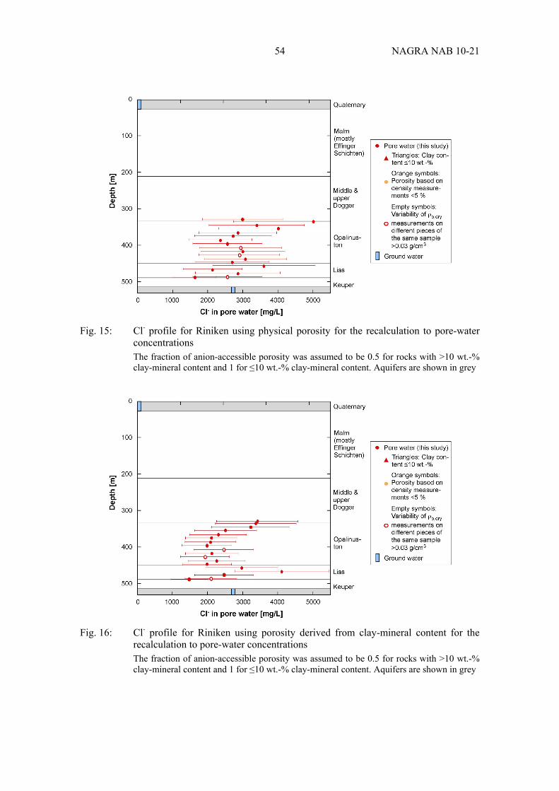
54 NAGRA NAB 10-21

Fig. 15: Cl- profile for Riniken using physical porosity for the recalculation to pore-water concentrations The fraction of anion-accessible porosity was assumed to be 0.5 for rocks with >10 wt.-% clay-mineral content and 1 for ≤10 wt.-% clay-mineral content. Aquifers are shown in grey

Fig. 16: Cl- profile for Riniken using porosity derived from clay-mineral content for the recalculation to pore-water concentrations The fraction of anion-accessible porosity was assumed to be 0.5 for rocks with >10 wt.-% clay-mineral content and 1 for ≤10 wt.-% clay-mineral content. Aquifers are shown in grey

55 NAGRA NAB 10-21

Fig. 17: Cl- profile for Schafisheim using physical porosity for the recalculation to pore-water concentrations The fraction of anion-accessible porosity was assumed to be 0.5 for rocks with >10 wt.-% clay-mineral content and 1 for ≤10 wt.-% clay-mineral content. Aquifers are shown in grey

Fig. 18: Cl- profile for Schafisheim using porosity derived from clay-mineral content for the recalculation to pore-water concentrations The fraction of anion-accessible porosity was assumed to be 0.5 for rocks with >10 wt.-% clay-mineral content and 1 for ≤10 wt.-% clay-mineral content. Aquifers are shown in grey

56 NAGRA NAB 10-21

Fig. 19: Cl- for profile Weiach using physical porosity for the recalculation to pore-water concentrations The fraction of anion-accessible porosity was assumed to be 0.5 for rocks with >10 wt.-% clay-mineral content and 1 for ≤10 wt.-% clay-mineral content. Aquifers are shown in grey

Fig. 20: Cl- profile for Weiach using porosity derived from clay-mineral content for the recalculation to pore-water concentrations The fraction of anion-accessible porosity was assumed to be 0.5 for rocks with >10 wt.-% clay-mineral content and 1 for ≤10 wt.-% clay-mineral content. Aquifers are shown in grey

57 NAGRA NAB 10-21

Fig. 21: Screened Cl- profile for Benken using porosity derived from clay-mineral content for the recalculation to pore-water concentrations The fraction of anion-accessible porosity was assumed to be 0.5 for rocks with >10 wt.-% clay-mineral content and 1 for ≤10 wt.-% clay-mineral content. Only the screened data set is shown, together with a polynomial fit. Waber et al.'s (2003) data (blue squares) are left as in the original, i.e. they refer to water-loss porosity and an anion-accessible porosity fraction of 0.5

Fig. 22: Screened Cl- profile for Riniken using porosity derived from clay-mineral content for the recalculation to pore-water concentrations The fraction of anion-accessible porosity was assumed to be 0.5 for rocks with >10 wt.-% clay-mineral content and 1 for ≤10 wt.-% clay-mineral content. Only the screened data set is shown, together with a polynomial fit

58 NAGRA NAB 10-21

Fig. 23: Screened Cl- profile for Schafisheim using porosity derived from clay-mineral content for the recalculation to pore-water concentrations The fraction of anion-accessible porosity was assumed to be 0.5 for rocks with >10 wt.-% clay-mineral content and 1 for ≤10 wt.-% clay-mineral content. Only the screened data set is shown, together with a polynomial fit

Fig. 24: Screened Cl- profile for Weiach using porosity derived from clay-mineral content for the recalculation to pore-water concentrations The fraction of anion-accessible porosity was assumed to be 0.5 for rocks with >10 wt.-% clay-mineral content and 1 for ≤10 wt.-% clay-mineral content. Only the screened data set is shown, together with a polynomial fit

59 NAGRA NAB 10-21

7 References

Bruland, K.W. & Lohan, M.C. 2003. Controls of trace metals in seawater. In: H.D. Holland & K.K. Turekian (eds) Treatise on Geochemistry, vol. 6 (The oceans and marine geochemistry), 23-47

Füchtbauer, H., 1988. Sedimente und Sedimentgesteine. Schweizerbart Verlagsbuchhandlung, Stuttgart, Germany

Gimmi, T. & Waber, H.N. 2004. Modelling of tracer profiles in pore water of argillaceous rocks in the Benken borehole: Stable water isotopes, chloride and chlorine isotopes. Nagra Tech. Rep. NTB 04-05

Gimmi, T., Waber, H.N., Gautschi, A. & Rübel, A. 2007. Stable water isotopes in pore water of Jurassic argillaceous rocks as tracers for solute transport over large spatial and temporal scales. Water Resources Research 43, W04410

Koroleva, M., Alt-Epping, P. & Mazurek, M. 2011. Large-scale tracer profiles in a deep claystone formation (Opalinus Clay at Mont Russelin, Switzerland): implications for solute transport processes and transport properties of the rock. Chemical Geology 280, 284-296

Mäder, U. 2009a. Reference pore water for the Opalinus Clay and "Brown Dogger" for the provisional safety-analysis in the framework of the sectoral plan - interim results (SGT-ZE). Nagra Arbeitsber.

Mäder, U. 2009b. Reference pore water for the Effingen Member (Standortregion Südjura) for the provisional safety-analysis in the framework of the sectoral plan - interim results (SGT-ZE). Nagra Arbeitsber.

Matter, A., Peters, T., Isenschmid, C., Bläsi, H.R. & Ziegler, H.J. 1987. Sondierbohrung Riniken – Geologie. Nagra Tech. Ber. NTB 86-02

Matter, A., Peters, T., Bläsi, H.R., Meyer, J., Ischi, H. & Meyer, C. 1988a. Sondierbohrung Weiach – Geologie. Nagra Tech. Ber. NTB 86-01

Matter, A., Peters, T., Bläsi, H.R., Weiss, H.P. & Schenker, F. 1988b. Sondierbohrung Schafisheim – Geologie. Nagra Tech. Ber. NTB 86-03

Mazurek, M. 2011. Aufbau und Auswertung der Gesteinsparameter-Datenbank für Opalinuston, den "Braunen Dogger", Effinger Schichten und Mergel-Formationen des Helvetikums. Nagra Arbeitsber.

Mazurek, M., Hurford, A. J. & Leu, W. 2006. Unravelling the multi-stage burial history of the Swiss Molasse Basin: Integration of apatite fission track, vitrinite reflectance and biomarker isomerisation analysis. Basin Research 18, 27-50

Mazurek, M., Alt-Epping, P., Bath, A., Gimmi, T. & Waber, H. N. 2009. Natural tracer profiles across argillaceous formations: The CLAYTRAC project. OECD/NEA report 6253, OECD Nuclear Energy Agency, Paris, France

60 NAGRA NAB 10-21

Mazurek, M., Meier, D. & Müller, H. 2010. WS-H experiment: Geological, petrophysical and geochemical characterisation of drillcores from borehole BHG-B11. Mont Terri Technical Note TN 2010-22, Mont Terri Consortium, St. Ursanne, Switzerland

Mazurek, M., Alt-Epping, P., Bath, A., Gimmi, T., Waber, H. N., Buschaert, S., De Cannière, P., De Craen, M., Gautschi, A., Savoye, S., Vinsot, A., Wemaere, I. & Wouters, L. 2011. Natural tracer profiles across argillaceous formations. Applied Geochemistry 26, 1035-1064

Nagra 1988. Sondierbohrungen Böttstein, Weiach, Riniken, Schafisheim, Kaisten Leuggern: Fluid Logging - Temperatur-. Leitfähigkeits- und Spinner-Flowmeter-Messungen. Nagra Tech. Ber. NTB 85-10

Nagra 1989. Sondierbohrung Weiach: Untersuchungsbericht. Nagra Techn. Ber. NTB 88-08

Nagra 1990. Sondierbohrung Riniken: Untersuchungsbericht. Nagra Tech. Ber. NTB 88-09

Nagra 1992. Sondierbohrung Schafisheim: Untersuchungsbericht. Nagra Tech. Ber. NTB 88-11

Nagra 2001. Sondierbohrung Benken: Untersuchungsbericht. Nagra Tech. Ber. NTB 00-01

Nagra 2002. Projekt Opalinuston - Synthese der geowissenschaftlichen Untersuchungs-ergebnisse. Nagra Tech. Ber. NTB 02-03

Nagra 2008. Vorschlag geologischer Standortgebiete für das SMA- und das HAA-Lager – Geologische Grundlagen. Nagra Tech. Ber. NTB 08-04

Pearson, F.J., Arcos, D., Bath, A., Boisson, J.Y., Fernandez, A.M., Gaebler, H.E., Gaucher, E., Gautschi, A., Griffault, L., Hernan, P., and Waber, H.N. 2003. Geochemistry of water in the Opalinus Clay formation at the Mont Terri Rock Laboratory - Synthesis Report. Swiss Federal Office for Water and Geology (FOWG), Bern, Switzerland, Geology Series, Nr. 5

Waber, H.N., Pearson, F.J., Hobbs, M.Y. & Oyama, T. 2003. Sondierbohrung Benken: Characterisation of pore water from argillaceous rocks. Nagra Intern. Ber.