VERTICAL PRICE TRANSMISSION IN THE EGYPTIAN TOMATO SECTOR AFTER THE

ARAB SPRING

Osama Ahmed1 and Teresa Serra

2

1Centre de Recerca en Economia i Desenvolupament Agroalimentaris (CREDA)-

UPC-IRTA, Parc Mediterrani de la Tecnologia, Edifici ESAB,

C/ Esteve Terrades 8, 08860 Castelldefels, Spain.

2Department of Agricultural and Consumer Economics (ACE), University of Illinois, 335 Mumford

Hall, 1301 W Gregory Drive, Urbana, IL 61801.

Abstract

This study assesses price transmission along the Egyptian tomato food marketing chain in the

period that followed the Arab Spring, which accentuated economic precariousness in Egypt. Static

and time-varying copula methods are used for this purpose. Results suggest a positive link between

producer, wholesaler and retailer tomato prices. Such positive dependence is characterized by

asymmetries during extreme market events, that lead price increases to be transferred more

completely along the supply chain than price declines.

Keywords: food prices, asymmetric price transmission, dependence analysis, static and time-

varying copula.

JEL codes: C5, Q11, Q12, Q18.

1. Introduction

The prevailing economic situation in Egypt before the 2011 Arab Spring was

challenging and partly characterized by high unemployment rates, specially among

youth, unfair wage structures, and high food and energy prices. The revolutions

accentuated economic precariousness: GDP growth rates decreased from 5.1% in 2010

to 2.2% in 2012, while inflation measured through the consumer price index grew by

9.5% in 2013 (World Bank, 2013). Price increases are bigger if a longer time span is

considered: from the 1st week of January 2011 till the 1

st week of December 2013,

Egyptian food prices increased by 17.7% (Egyptian Food Observatory, 2013).

This economic downturn led to food price instability, food shortages and higher

poverty. In 2013, more than 79% of family income was spent on food and more than

80% of Egyptian population earned insufficient income to cover consumption needs.

According to the Egyptian Center for Economic and Social Rights (ECESR, 2013), the

poverty rate increased from 21.6% in 2008/2009 to 26.3% in 2012/2013. Rising poverty

worsened food insecurity that increased from 14% of the Egyptian population in 2009 to

17.2% (13.7 million people) in 2011 (ECESR, 2013). Undernourishment, on the other

hand, represented more than 5% of Egyptian population in the 2011-2013 period (Africa

Food Security and Hunger, 2014).

Egyptian consumers have used different strategies to cope with recent food price

increases: food purchases have been curbed down by 12.2% and more than 26% of

consumers have opted for lower quality food products at cheaper prices (Egyptian Food

Observatory, 2013). Prevention of malnutrition implies ensuring access to food at fair

consumer prices. Assessing food consumer price formation requires analyzing how food

prices are transmitted along the food marketing chain, from agricultural producers to

final consumers. The objective of this research article is to shed light on this matter by

focusing on the tomato sector in Egypt.

Understanding price behavior along the food marketing chain is very useful to

assess the functioning of food production, processing and distribution markets, their

competition and integration level. Vertical price transmission analyses can help

identifying market failures and are a good indicator of the degree of competitiveness

and effectiveness of market performance. Competitive behavior is rare in less developed

countries (LDCs) due to different market characteristics such as excessive governement

1

intervention, corruption, defficient infrastructures, etc. Since prices drive resource

allocation and production decisions, price transmission information is useful for

economic agents when taking their economic decisions, policy makers and competition

regulatory authorities. Hence, the link between different prices at different levels of the

food marketing chain is a very interesting research topic in LDCs. This article

characterizes the relationship between producer and wholesaler price levels, and

between wholesaler and consumer price levels of tomato markets in Egypt. The analysis

is of a pair-wise nature. Pair-wise analyses are usual in the price transmission literature

and represent a natural avenue for studying price relationships (Goodwin and Piggott,

2001). Lack of food price data in LDCs is the reason underlying the scarcity of studies

on price behavior in these countries. This makes the contribution of the proposed

analysis an even more appealing one.

Sound assessment of price links requires knowledge of the joint distribution of the

prices considered. Under the assumption that the joint price distribution is Gaussian or

t-Student, methods such as vector autoregressive or error correction type of models have

been widely used. Univariate distributions of economic time series are usually found to

be characterized by excess kurtosis, skewness and nonnormality. Further, related price

series may show asymmetric dependence, which is an indicator of multivariate

nonnormality (Patton, 2006). As a result, the Gaussian and the t-Student distributions

have been shown as inappropriate to assess behavior of the type of data we intend to

study. Inadequate assumptions of multivariate distributions will lead to biased

parameter estimates. Further, since the range of available multivariate distributions is

limited, this limits how multivariate dependence can be modeled (Parra and Koodi,

2006).

Assessment of dependence between producer, wholesaler, and retailer levels

should be based on flexible instruments that soundly capture the joint distribution

function of the variables considered. Recent research has suggested the use of statistical

copulas as an alternative. Copulas are statistical instruments that combine univariate

distributions to obtain a joint distribution (multivariate distribution) with a particular

dependence structure. A key advantage intrinsic to copulas is that they are based on

univariate distributions, instead of multivariate ones. This is specially important given

the scarcity of multivariate distributions available from the statistical literature.

This paper is organized as follows. In the next section, a brief description of the

tomato market in Egypt is offered. In section 3, a literature review of vertical price

2

transmission analyses using time-series econometric techniques is presented. In section

4, the methodological approach is described. The fifth section is devoted to the

empirical implementation to assess dependence between producer and wholesaler, and

between wholesaler and retailer prices. The last section in this article offers the

concluding remarks.

2. Tomato market in Egypt

World production of vegetables in 2012 was 1.1 billion tons on an extension of land of

57.2 million hectares. Africa produced 74.1 million tons, representing an increase on the

order of 86.5% relative to 2006 and more than 6.5% of worldwide production

(FAOSTAT, 2012). Among African countries, Egypt vegetable production expanded

from 18.3 million tons in 2006 (FAOSTAT, 2006) to 19.8 million tons in 2012,

representing an increase of around 8.2% (FAOSTAT, 2012) and around 26.7% of all

vegetables produced in Africa. According to the International Trade Center (ITC), in

2011 edible vegetables global exports and imports were on the order of 66.5 and 65.4

million tons, respectively (ITC 2011). In the same year, African vegetables exports and

imports were 4.6 and 6.1 million tons, respectively (FAOSTAT, 2011).

Tomato is the most relevant vegetable in terms of world production and

consumption (FAOSTAT, 2012). Global tomato production expanded from 131.3

million tons in 2006 (FAOSTAT, 2006) to 161.7 million tons in 2012 (FAOSTAT

2012). More than 30% of tomato production is used by the processing industry. In 2012,

international exports and imports of tomato were estimated to be 7.1 and 6.9 million

tons, respectively (ITC, 2012). Tomato production is distributed among 170 countries,

being Egypt the fifth largest global producer after China, India, United States, and

Turkey. These five countries represent around 62% of total world tomato production

(FAOSTAT, 2012). Tomato is extremely important for African economies that in 2012

devoted 21.5 million hectares to produce 17.9 million tons, representing 24.19% of the

vegetables produced in Africa (FAOSTAT, 2012). African exports (imports) of tomato

were estimated to be on the order of 535.3 (60) thousand tons in 2011 (FAOSTAT,

2011).

Tomato is the first vegetable in terms of consumption and production in Egypt.

While food consumption patterns involve a frequency of vegetables consumption of 6.5

days a week, tomato is consumed, on average, 5.8 days a week (Egyptian Food

Observatory, 2013). In 2012, tomato harvest in Egypt exceeded 8.6 million tons, grown

3

on more than 216 thousand hectares, representing 28% of the area cultivated with

vegetable crops (FAOSTAT, 2012). Egypt, with half of tomato production, is the largest

producer in Africa (FAOSTAT, 2012). Egyptian exports of tomato were 62.2 thousand

tons in 2011, and the main destinations were the Kingdom of Saudi Arabia, Netherlands

and United Kingdom. Egyptian tomato imports were 5.3 thousand tons (ITC, 2012).

More than 30% of the domestic tomato production is processed by 14 companies into

tomato paste and other products

Income derived from tomatoes fluctuates highly, mainly due to price

instabilities. Net returns in 2007 were on the order of 170 US$ per feddan. In winter

2011/2012, net returns increased to 3,000 US$ per feddan, and decreased to be 1,200

US$ feddan in the summer 2012 (USDA, 2014). While tomatoes are grown in Egypt

throughout the year in different regions, most production occurs in the Upper Egypt,

especially in the governorate of Qena (SIS, 2013). Most production is channeled

through two main wholesale markets in Egypt: El Abour market in Cairo and El Hadra

market in Alexandria, and subsequently distributed to retail markets after tomatoes have

been sorted, processed, and repackaged.

Small and poor tomato producers suffer from low yields and high income

instability. Further, they often rely on the black market, where prices are usually very

high, to acquire their inputs (Boutros, 2014). After the implementation of the public-

private partnership between USAID, ACDI-VOCA, Heinz International and 13

domestic tomato processors, in order to improve economic sustainability of small

tomato producers, producers sell 30% of their production through forward contracts to

processor companies. This increases the range of market outlets reducing wholesaler

market power (USDA, 2014).

3. Literature review

According to their methodological approach, price transmission analyses can be

classified into structural and non-structural studies. While structural models rely on

economic theory, non-structural analyses identify empirical regularities in the data. Our

approach to studying price transmission along the Egyptian marketing chain is based on

non-structural time-series models. Time series data often violate the most common

assumptions of conventional statistical inference methods, which may lead to obtaining

completely spurious results. Cointegration and error correction models (ECM) have

been introduced in the literature (Engle and Granger, 1987) to characterize

4

nonstationary and cointegrated data and inform both on their short and long-run time-

variation. Time-varying and clustering volatility, another common characteristic of

time-series, is typically modeled through generalized autoregressive conditional

heteroskedasticity (GARCH) models.

The work by Chang (1998) relies on Engle and Granger (1987) cointegration

techniques, to study long run relationships among Australian beef prices at the farm,

wholesale and retail levels. Evidence is found that all three prices are non stationary and

maintain a long-run equilibrium relationship, being the retail price the one that drives

price patterns. Price time series may also be characterized by asymmetric adjustment to

long-run equilibrium. Recent literature in this area has relied on smooth transition or

discrete threshold time-series models that usually allow for autoregressive and error

correction patterns. The work by Abdulai (2002) analyzes the relationship between

producer and retail pork prices in Switzerland, by employing threshold cointegration

tests. Results indicate that price transmission between producer and retail market levels

is asymmetric, since increases in producer prices are transferred more rapidly to

retailers than producer price declines. Using an asymmetric error-correction model, Von

Cramon-Taubadel (1998) obtains the same results for the German pork market. Vavra

and Goodwin (2005) use threshold vector error correction models (TVECM) to appraise

the links between retail, wholesale and farm level prices for the US beef, chicken and

egg markets. Research results indicate that there are significant asymmetries, both in

terms of speed and magnitude of the adjustment, in response to positive and negative

price shocks. Evidence of asymmetric price transmission along the food marketing

chain is also found by Seo (2006), Saikkonen (2005), Goodwin and Holt (1999), Serra

and Goodwin (2003), Meyer and von Cramon-Taubadel (2004), among others.

TVECM are used by Pozo et al. (2011) to examine price transmission among

farm, wholesale and retail US beef markets. Results show that there is no evidence of

asymmetric price transmission in any of the models. To the best of our knowledge, the

work by Gervais (2011) is the first paper focusing on potential nonlinearities in both the

long- and short-run. Gervais (2011) studies the US pork marketing chain, from farm to

consumer markets. Results indicate the importance of testing for linearity in the long-

run relationship between prices. Results also show that a decrease in farm prices is

eventually transferred to consumers.

There are few studies that have addressed vertical price transmission along the

food chain in developing countries. Guvheya et al. (1998) assess vertical price

5

transmission in Zimbabwe tomato market using causality and Houck (1977) methods.

Price transmission between farm and wholesale market levels is characterized by price

asymmetries, but price transmission from wholesale to retail markets is symmetric. Iran

horticultural markets (date and pistachio) have been studied by Moghaddasi (2008).

Houck (1977) approach is used to characterize the pistachio market and ECM the date

market. Results indicate that there is asymmetry in price transmission from farm to

retail markets. Granger and Lee (1989) asymmetric ECM is used by Acquah (2010) to

examine and confirm existence of asymmetry in price transmission between wholesaler

and retailer maize prices in Ghana.

Negassa (1998) focuses on vertical price transmission in grain markets in

Ethiopia by using correlation coefficients and casualty methods and finds evidence of

symmetries. Minten and Kyle (2000) examines price asymmetry in urban food markets

in Zair. Evidence is found that prices are symmetrically passed between producer and

wholesaler market levels, but transmitted asymmetrically between wholesaler-retailer

markets. Alam et al. (2010) apply an ECM on rice market prices in Bangladesh. Prices

along the chain are positively linked and wholesalers set market prices. Evidence of

asymmetric price transmission is also found.

More recently, other methodological approaches based on the use of statistical

copulas have started to gain interest among economists interested in price transmission

analyses. These methods rely on direct examination of the joint probability distribution

function of the variables that are being studied and pay special attention to the nature of

jointness between these variables. The work by Serra and Gil (2012) studies dependence

between two pairs of prices: crude oil and biodiesel blend prices, and crude oil and

diesel prices in Spain, with a special focus on this dependence during extreme market

events. Statistical copulas are used for such purpose. Results prove asymmetric

dependence between crude oil and biodiesel prices, which protects consumers against

extreme crude oil price increases. Diesel prices, in contrast, equally reflect crude oil

price increases and decreases. The work by Goodwin et al. (2011) studies the joint

distribution of North American lumber prices in different markets (Eastern Canada,

North Central US, Southeast US, Southwest US). Copula models are used to obtain the

correlation between prices at the geographical locations considered. Results indicate

that market adjustments are generally larger in response to large price differences which

reflect more substantial disequilibrium conditions.

6

The unpublished article by Qiu and Goodwin (2013) relies on the application of

static and time-varying copula models to the empirical study of the links between farm-

retail and retail-wholesale prices for US hog/pork markets. Results indicate that farm

and wholesale markets are closely related to each other, while retail price adjustment is

less dependent on the other two markets. Farm-retail and retail-wholesale price

adjustments have relatively constant dependence structures. Also, results confirm the

existence of time-varying and asymmetric behavior in price co-movements between

farm and retail markets. Positive upper and zero lower tail dependencies provide

evidence that big increases in farm prices are matched at the retail level, while negative

shocks at the farm level are less likely to be passed to consumers.

Our paper contributes to the literature by assessing dependence between

producer-wholesaler and wholesaler-retailer price levels in tomato markets in Egypt.

During the political transition period, Egypt suffered from food insecurity and food

price instability. It is thus important to pay special attention to extreme upturns and

downturns of the tomato market, as these are likely to have a stronger impact on food

security and economic issues. Since we assess a period of important changes, not only

static, but also time-varying copulas are used in order to allow for changes in price

patterns. To our knowledge, this is the first attempt to study vertical price transmission

in LCD countries using this methodology.

4. Methodology

Multidimensional copula functions are used to assess dependence between prices at

different levels along the tomato supply chain in Egypt. While copulas have been

widely used in the financial economics literature (Patton 2006, 2012; or Parra and

Koodi 2006), empirical studies that use copulas to assess dependency along the food

marketing chain are more scarce, even more so in developing economies. Statistical

copulas have the advantage of allowing high flexibility when studying correlation

between two or more variables. A copula function is a multivariate distribution function

defined on the unit cube 0, 1n, with uniformly distributed marginals. Copulas are

based on the Sklar’s (1959) theorem that shows how multivariate distribution functions

characterizing dependence between n variables, can be decomposed into n univariate

distributions and a copula function, the latter fully capturing the dependence structure

between variables.

7

Recall our analysis is of a pairwise nature. Let xF and yF be the univariate

distribution functions of two random variables ( , )x y . ( , )H x y is assumed to represent

the joint distribution function. According to the Sklar’s theorem, there exists a copula

.C that can be expressed as (Embrechts et al., 2001):

( , ) ( ( ), ( )) ( , )x yH x y C F x F y C u v , (1)

where .C is a 2-dimensional distribution function with uniformly distributed margins

(0,1) and (0,1)u Unif v Unif . The joint density function can be defined as:

( , ) ( ) ( ) ( , )x yh x y f x f y c u v , (2)

where c is the copula density and ( )xf x and ( )yf y are the univariate density functions

of the random variables.

Different copula families and specifications represent different dependence

structures. Our analysis will consider both elliptical (Gaussian and Student’s t copulas)

and Archimedean (Gumbel, Symmetrized Joe-Clayton-SJC copulas) copulas. Elliptical

copulas are based on the elliptical distribution, while Archimedean are a group of

associative copulas that have the advantage of reducing dimensionality issues during the

estimation process. Copulas may also be categorized as static and time-varying. A static

copula implies parameter constancy over time, while a time-varying copula allows the

parameters to change with changing environment. In order to ensure that the copulas

correctly fit our data, a series of time-varying dependence and goodness of fit (GoF)

tests are conducted. As a result, price dependency along Egyptian tomato marketing

chain is modeled using four copulas. The Gaussian copula is selected for being the

benchmark copula in economics. The Gumbel, the Student’s t, and the SJC copula are

selected based on statistical selection criteria (the log-likelihood value and goodness of

fit statistics described below).

The bivariate Gaussian copula can be expressed as:

8

12

1 1( ) ( )

2 212

221212

( , ; )( 2 )1

exp2 12 1

u vGaR Ru v

r R rs sC drds

RR

, (3)

where 12R is the correlation coefficient of the corresponding bivariate normal

distribution, 12 11 R , and denotes the univariate normal distribution function. A

drawback of the Gaussian copula is that it assumes that variables u and v are

independent in the extreme tails of the distribution. Hence, the Gaussian copula does not

allow for lower and upper tail dependence. It thus represents dependence in the central

region of the distribution. The implication for our analysis is that the Gaussian copula

assumes that price transmission along the food market chain does not occur for very

high/low market prices.A bivariate student’s t copula can be expressed as:

1 1

( 2)/2

2 2( ) ( )12

, 221212

21( , ) exp 1

12 1

t u t vt

R

r R rs sC u v drds

RR

, (4)

where 12R is the correlation coefficient of the corresponding bivariate t-distribution

with degrees of freedom (as explained by Embrechts et al. 2001, 2 for the

correlation to be defined), and t

denotes the bivariate distribution function. When

30 , the Student’s t copula tends to the Gaussian copula (Goodwin 2012). The

student’s t copula assumes positive and symmetric lower and upper tail dependence.

The Gumbel copula can be expressed as (Manner 2007):

1/

ln ln( , ) expGu u vC u v

. (5)

This copula measures right tail dependence, which can be expressed as 1/2 2r

, but

assumes left tail dependence to be 0l . In terms of our case analysis, this copula

relies on the assumption that price transmission between different market levels only

takes place for high market prices. The Joe-Clayton copula can be expressed as:

9

1/

,

1/

1 1 1 1 1 1( , ) 1

U L

k k

k

jc u vC u v

(6)

where 21/ log (2 )Uk ,

21/ lo ( )g L , (0,1)U , and (0,1)L . Joe-Clayton

copula has two parameters, U and L , that measure the upper and lower tail

dependence, respectively. This copula characterizes tail dependency, i.e., it models price

behavior during extreme events. As noted in the literature review above, evidence of

asymmetries in vertical price transmission within the food marketing chain is abundant.

These asymmetries tend to be more pronounced as we move to extreme tails of the

distribution (i.e., when price increases or declines are larger), which we capture through

the static symmetrized Joe-Clayton (SJC) specification. More specifically, this copula

models the probability that relevant increases (declines) in the prices studied occur

together. The Joe-Clayton copula implies asymmetric dependence, even when U =

L .

The Symmetrized Joe-Clayton (SJC) copula allows overcoming this problem (Patton,

2006) and can be specified as:

, , ,( , ) 0.5 ( , ) (1 ,1 ) 1U L U L U L

sjc jc jcC u v C u v C u v u v

. (7)

Use of time-varying copulas was seen to be necessary after some testing

procedures that will be discussed below. Hence, dependency during the period studied

was not found to remain constant. The dynamic Student’s t copula and SJC copula were

chosen, on the basis of the highest log-likelihood values, to capture dependency

changes. Time-varying versions of Student’s t copula define the correlation parameter to

evolve through time as shown in equation (8) below (Patton, 2006):

1

101 1

1

1

10tt t i t i

i

t u t v

(8)

where 1t

is the inverse of the t distribution of t with degrees of freedom, and

1(1 ) xe is the modified logistic function. The time-varying version of the SJC

copula is defined following Patton (2006):

10

1

10

1

1

10t

U U

t U U U t i t i

i

u v

, (9)

1

10

1

1

10t

L L

t L L L t i t i

i

u v

(10)

where 1(1 ) xe denotes the logistic transformation that keeps the upper and lower

tails ( U

t , L

t ) in the (0, 1) range.

Copulas can be estimated through two stage estimation processes. The first stage

consists of estimating marginal models that filter information contained in univariate

distributions and allow deriving standardized, independent and identically distributed

(i.i.d.) residuals from the filtration. The copula is estimated in a second stage either

through parametric or non-parametric methods. We use the latter, that consist of

transforming the i.i.d. residuals into (0,1)Unif using the non-parametric empirical

cumulative distribution function (EDF). The empirical EDF method is especially

convenient when the true distribution of the data is not known. The maximum

likelihood method is applied on the uniform residuals to estimate copula parameters.

The two-stage estimation technique can be formalized as follows (Patton, 2012):

1

1

argmax log ( ; ),

argmax log ( ; ),

1

1

u

v

u

v

T

ui jj

T

vi jj

f u

f v

T

T

(11)

1

argmax ( ( ; ), ( ; ); ).log1j u j v

T

j

F u F vcT

(12)

where u and v represent parameter estimates of marginal distributions and is the

copula estimated parameter vector. Since the theory of copulas applies on stationary

time-series, tests for unit roots are run on our data. Results support the absence of a unit

root in producer, wholesaler and retailer prices.

Univariate ARMA(pa,qa)-GARCH(pg,qg) marginal models capture univariate

price patterns with pa representing the number of autoregressive parameters of the

ARMA model; qa the number of moving average components, pg the number of

autoregressive terms in the GARCH specification and qg the number of lags of squared

11

innovations. ARMA models price-level behavior as a function of autoregressive and

moving average terms. Residuals are modeled through GARCH specification in order to

allow for time-varying and clustering volatility:

1 2

1 1

pa qa

i i t

i i

t t i t iP c P

(13)

1 1

2 2 22 1

pg qg

i i

t i t i t ii i

(14)

where tP are the prices considered, c is the constant of the conditional mean model,

1i is the coefficient representing the autoregressive component, 2i is the coefficient

representing the moving average component, being t a normally distributed error

term, i is the constant in the conditional volatility model, being 1i

and 2i

the

coefficients representing the lagged square residuals and variance, respectively.1 Log-

likelihood methods assuming normally distributed errors are used in model estimation.

Two types of time-varying dependence tests are used to determine whether time-

varying copulas need to be considered (Patton, 2013). The first focuses on rank

correlation breaks between u and v at some unknown date and is based on the “sup” test

statistic (Patton, 2013):

* * *sup 1, 2,,

maxL U

t tt t t

B

, (15)

where

*

* 1*1,1

123

t

t t ttt

u vt

and

*

* 1*2,1

123

t

t t ttt

u vT t

. In order to have enough

observations to estimate the pre- and post-break parameters, the interval * *[ , ]L Ut t is

usually defined as[0.15 ,0.85 ]T T , where T is the number of observations. The critical

value of supB can be determined through a bootstrap process defined in Patton (2013).

The second test is the ARCH LM test for time-varying volatility (Engle, 1982). This test

focuses on autocorrelation in dependence, captured by an autoregressive model such as

the following:

1

The univariate model was specified according to parsimony and statistical significance.

12

0

1

p

t t i t i t i t

i

u v u v e

, (16)

where te is the error term. The null of a constant copula implies 0, 1i i , which

can be tested through the following statistic:

1

ˆ ˆˆ ˆpA R RV R R

, (17)

where0

ˆ ,......, p , 10p pR I

and V̂ is the OLS estimate for the covariance

matrix. A bootstrap process described in Patton (2013) is used to determine the test

critical values.

Goodnes of fit (GoF) tests are used to assess to what extent an estimated copula

model is different from the unknown true copula. Comparison of estimated with

unknown copula is made through the Kolmogorov-Smirnov (KSc) and the Cramer-von-

Mises (CvMc) tests (Genest and Rémillard 2008, 2009; and Rémillard 2010). These

tests can be expressed as follows:

ˆ ˆmax ( , ; ) ( , )T Tt

KSc C u v C u v (18)

2

1

ˆ ˆ( , ; ) ( , )T

T T

t

CvMc C u v C u v

. (19)

The empirical copula has been often used to provide a nonparametric estimate of

the true unknown copula. However, the empirical copula is not a valid approach when

the true underlying copula is time-varying. The problem can be addressed by using the

fitted copula to derive a Rosenblatt (1952) transform of the data that yields a vector of

i.i.d. mutually independent Unif (0,1) variables. The GoF tests are then computed as:

ˆ ˆmax ( , ; ) ( , )T Tt

KSr C u v C u v (20)

2

1

ˆ ˆ( , ; ) ( , )T

T T

t

CvMr C u v C u v

(21)

13

where u and v are the Rosenblatt transformations. Rémillard (2010) proposes a

bootstrap process in order to determine the critical values for tests KSc and CvMc .

Patton’s (2013) recommendation is followed to obtain the critical values of KSr and

CvMr .

Conducting goodness of fit tests on the marginal models is essential for copula

model estimation. In order to make sure that the residuals obtained from univariate

models have no autocorrelation, the Ljung-Box tests are used. The LM tests of serial

independence of the first four moments of tu and tv are estimated by regressing

k

tu u and k

tv v on 10 lags for each price series, for k= 1,2,3,4. We also use the

Kolmogorov-Smirnov (KS) test to make sure that the transformed series are

(0,1)Unif (see Patton 2006 for further details).

5. Empirical analysis

The analysis is based on weekly tomato price data expressed in euro/kg, and observed

from the first week of April 2011 to the last week of March 2014, leading a total of 155

observations. Prices at different levels of the marketing chain have been collected: the

price received by producers and wholesalers and the price paid by consumers. The three

series are obtained from the Egyptian cabinet information and decision support center

(IDSC, 2013). Prices are expressed in Egyptian pound per kilo and studied in pairs.

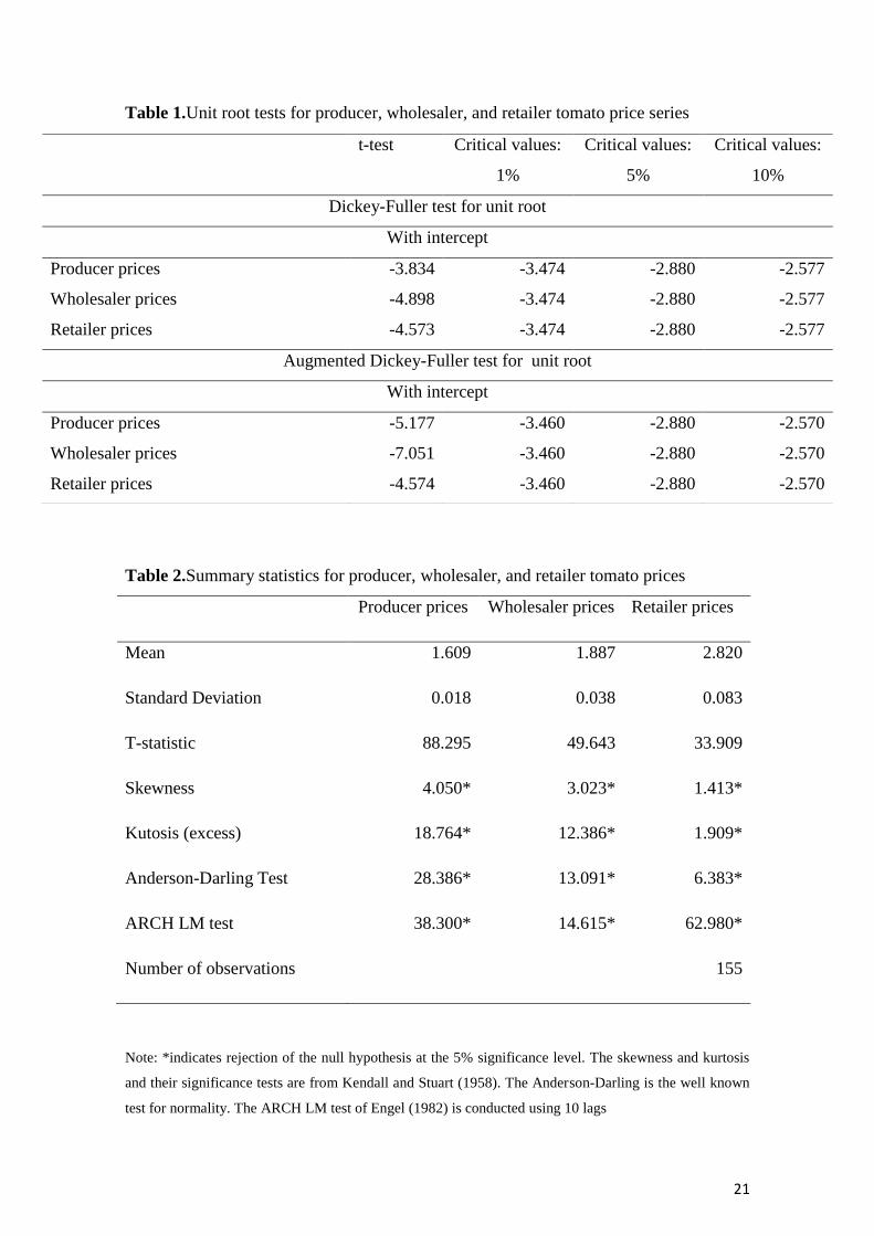
Standard unit root tests show that the series are stationary (Table 1). Table 2 presents

summary statistics for price series. These statistics provide evidence of non-normal

price series, characterized by skewness, kurtosis and ARCH effects.

Results from univariate ARMA-GARCH model, whose specification is chosen

through the Akaike’s information criterion (AIC) and Bayesian information criterion of

Schwarz’s (BIC), are presented in Table 3. An ARMA (1,4)-GARCH(1,1) model is fit

to producer and wholesaler prices, while an ARMA(2,2)-GARCH(1,1) better represents

retailer prices. Conditional mean model results suggest that current price levels are

positively influenced by price levels during the last week. Univariate GARCH (1, 1)

model parameter estimates are all positive for the three prices considered, which

indicates that past market shocks as well as past volatility bring higher current volatility

levels. Since 1 2 1i i , we can conclude that the three GARCH processes are

14

stationary, being the unconditional long-run variance 1 2

2 1i i ii around

0.022, 0.143, and 0.176 for producer, wholesaler, and retailer prices, respectively.

Hence, in the Egyptian tomato market, consumer prices have long-run volatilities that

are above the volatilities at the producer and wholesale price level.

The Ljung-Box test results presented in Table 3, allow accepting the null of no

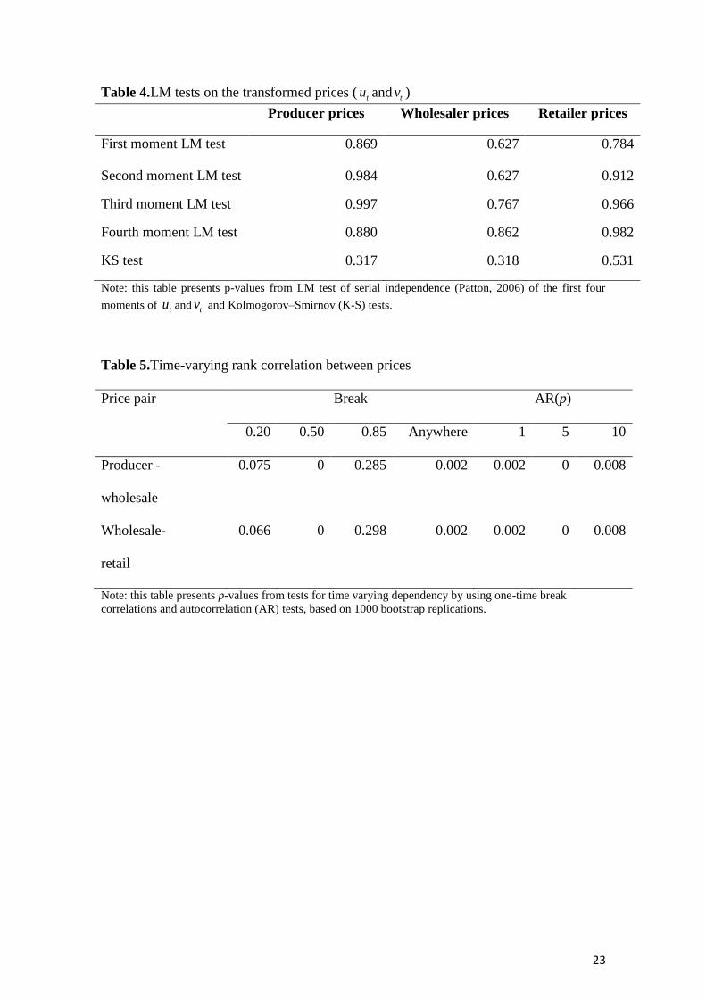
autocorrelated residuals. The LM tests (Table 4) implemented to check for the

independence of the first four moments of the transformed variables, provide evidence

that the models are well specified. The Kolmogorov–Smirnov (KS) test confirms that

the transformed series are Unif (0,1) (Patton 2006). Time-varying dependence tests in

Table 5 support the use of time varying copulas for both pairs of prices. In Table 6, we

present the log likelihood values for a wide range of copulas. Those copulas yielding the

highest log likelihood values are selected for a more in depth analysis. Gumbel,

Student-t, and SJC copula are chosen to represent dependency between both pairs of

prices (producer - wholesaler and wholesaler - retailer) . The Gaussian copula is also

chosen for both pairs of prices, as the benchmark model in economics.

Results of CKS and CCvM GoF tests (presented in Table 7) for producer –

wholesaler pair of prices suggest the Student´s t constant copula as the one providing

the best fit, being the second best fit provided by the Gaussian and the SJC constant

copulas. In the wholesaler – retailer case, the SJC constant copula offers the first best fit

and Student´s t constant copula the second best. For time varying copulas the GoF tests

suggest that the Student´s t better fits the data relative to SJC copula for both pairs of

prices. Given these results, static Gaussian, static and dynamic Student´s t, and static

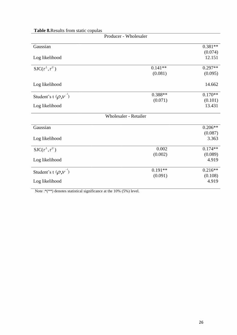
SJC copulas are considered in our analysis. Static copula results are presented in Table

8 and dynamic copula findings in Table 9, respectively.

Results of Gaussian and Student´s t copula presented in Table 8 imply a positive

short-run correlation between prices at different market levels. The association is

stronger between producer and wholesale prices, than between wholesale and retail

prices. Furthermore, the inverse of the degrees of freedom of Student’s t copulas are

0.170 and 0.216 for producer – wholesaler and wholesaler - retailer pairs of prices,

respectively. This implies strong dependence in the tail, which is not captured by the

Gaussian copula. It is thus relevant to estimate a copula that allows for dependency for

very high/low market prices.

15

Results of SJC copulas provide support for asymmetric dependency during

extreme market events. The SJC copula for the producer – wholesaler price pair shows

stronger (52% higher) upper than lower tail dependency, which suggests that price

increases tend to be passed from producers to wholesalers more completely than price

declines. For the wholesaler - retailer price pair, the lower tail is not statically different

from zero. Conversely, the upper tail is statistically significant and on the order of 0.13,

which implies that while price increases will be transferred from wholesalers to

retailers, price declines will be not. Hence, retailers are more likely to increase prices

than to reduce them, which reflects the degree of market power that retail chains have in

Egypt.

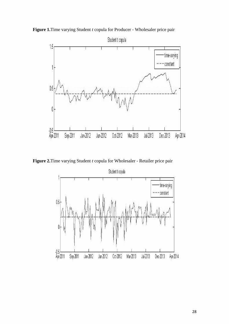
Time varying student’s t copula shows how dependency among the pairs of prices

considered changes over time. Estimation results are presented in Table 9 and graphed

in Figure 1 for the producer-wholesaler price pair, indicating that dependence from

April 2011 to March 2013 was relatively low and fluctuated around 0.4. In the period

from March 2013 to December 2013, dependence increased reaching values around 0.8.

Such increase is likely to be related to the project involving USAID, ACDI-VOCA,

Heinz International and 13 domestic tomato processors, to promote high quality and

consistent tomato production. Another aim of this partnership is to increase trust

between producers and tomato processors and stabilize their relationships through

forward contracts. Under these contracts, more than 30% of tomato production is

currently sold to processor companies, increasing tomato market outlets and reducing

wholesaler market power in Egypt (USDA 2014). This has led wholesalers to offer

higher prices to entice producers to sell tomatoes to them. The reduction of wholesaler

market power has led to increased dependency between producer and wholesaler market

levels, which is an indicator of more competitive market behavior. Time varying

Student’s t tail dependence displayed in Figure 2 shows a low dependency between

wholesaler and retailer market levels, which is on the order of 0.2, that fluctuates over

the period studied, mainly in the range from 0 to 0.4. Low dependency between

wholesaler and retailer prices may be explained by lack of a competitive structure

linking wholesalers and retailers. Fluctuations are not surprising given the economically

tumultuous period studied.

16

6. Concluding remarks

Food price analyses along the food chain have started to gain relevance in developing

economies as data are becoming available. These analyses are of high political, social

and economic interest, especially in light of low income levels and chronic poverty

affecting these countries. Egypt suffers from high food prices since the food price crisis

in 2007/2008. The revolution of January 25, 2011 came to accentuate price increases.

Our analysis focuses on tomato prices dependency along the Egyptian supply

chain. To do so, we use flexible methods that do not require assumption of restrictive

multivariate distribution functional forms. Copula techniques represent a flexible way to

study price dependency. In this context, we apply static and time-varying statistical

copulas to assess co-movements between two pairs of prices: producer – wholesaler and

wholesaler – retailer prices, both in the central and in the extreme regions of the

distribution. Results for the producer – wholesaler price pair, involve positive

dependence in the central region of the distribution. Further, extreme increases in

tomato producer price will be passed on to wholesaler price more completely than

producer price declines. Results from wholesaler – retailer price model also show a

positive dependence in the central region of the bivariate distribution, though less strong

than the one holding for the producer-wholesale price pair. Regarding dependency

during extreme market events, asymmetric dependence has been found by which

extreme increases in wholesale prices are passed on to retailer prices, while declines are

not. As a result, food consumers will not benefit from extreme declines in prices at

upper levels of the food chain, but they will have to endure extreme price increases.

Policies, such as provision of inputs at subsidized prices, or the promotion of

adoption of technological advances in the production of tomatoes, may imply reduced

production costs. Due to the presence of asymmetries, it is not however warranted that

this decline in costs will be transferred down the marketing chain until reaching

consumers. In order to combat food security in a country where famine is worrisome,

further actions down the marketing chain are required in order to increase the

competitive behavior of this chain and facilitate smooth price transmission. The lack of

competitive behavior in the nexus wholesaler - retailer levels is evidenced by a lower

degree of dependency between these two market levels. In this regard, initiatives that

reduce wholesaler and retailer market power will be useful, which involves increasing

the number of outlets both for unprocessed raw and processed tomatoes.

17

References

Abdulai, A., 2002. Using Threshold Cointegration to Estimate Asymmetric Price

Transmission in the Swiss Pork Market. App. Econ. 34, 679-687.

Acquah, H. D. G., 2010. Asymmetry in Retail-Wholesale Price Transmission for Maize:

Evidence from Ghana. American-Eurasian J. Agr. Environ. Sci. 7 (4): 452-456.

Africa Food Security and Hunger, 2014. Undernourishment Multiple Indicator

Scorecard. Available from

http://allafrica.com/download/resource/main/main/idatcs/00080509:c4065c2853

35e1a6173fa8bcceda7b41.pdf

Alam, M. J., Begum, I. A., Buysse, J., McKenzie, A. M., Wailes, E. J., Huylenbroeck,

G.V., 2010. Testing Asymmetric Price Transmission in the Vertical Supply

Chain in De-regulated Rice Markets in Bangladesh. Paper presented at the

American Association of Agricultural and Applied Economics 2010 AAEA,

CAES, & WAEA Joint Conference, Denver, Colorado, USA, July 25-27.

Boutros, I., 2014. The Egyptian and Californian tomato farmers and the galabaya mafia.

Daily News Egypt. June 28th

, 2014. Available from

http://www.dailynewsegypt.com/2013/09/30/the-egyptian-and-californian-

tomato-farmers-and-the-galabaya-mafia/

Dickey, D.A., Fuller, W.A. , 1979. Distribution of the estimators for autoregressive

time series with a unit root. J. Amer. Stat. Ass. 74, 427-431.

Egyptian Center for Economic and Social Rights (ECESR), 2013.Visualizing Rights: A

Snapshot of Relevant Statistics on Egypt. Factsheet No. 13. Available from

http://www.cesr.org/downloads/Egypt.Factsheet.web.pdf

Egyptian Food Observatory, 2013. Food Monitoring and Evaluation System. published

by the Egyptian Cabinet’s Information and Decision Support Center (IDSC) and

World Food Programme (WFP). Quarterly Bulletin, Issue 14, October-Decmber

2013. Available from http://documents.wfp.org/stellent/groups/public/

documents/ena/wfp263322.pdf

Embrechts, P., Lindskog, F., McNeil, A., 2001. Modeling Dependence with Copulas

and Applications to Risk Management. Department of Mathematics, Zurich.

Engle, R.F., 1982. Autoregressive conditional heteroscedasticity with estimates of the

variance of UK inflation. Economet. 50, 987-1007.

Engle, R.F., Granger, C.W.J., 1987. Cointegration and Error Correction:

Representation, Estimation, and Testing. Economet. 55, 251-276.

FAOSTAT, 2012. Food and Agriculture Organization of the United Nations. Dataset.

Available from http://faostat3.fao.org/faostat-gateway/go/to/download/Q/*/E.

18

FAOSTAT, 2011. Food and Agriculture Organization of the United Nations.

Dataset.Available from http://faostat3.fao.org/faostat gateway/go/to/ download

/Q/*/E.

FAOSTAT, 2006. Food and Agriculture Organization of the United Nations. Dataset.

Available from http://faostat3.fao.org/faostat-gateway/go/to/download/Q/*/E.

Gervais, J-P., 2011. Disentangling Non-linearities in the Long- and Short-run Price

Relationships: An Application to the US Hog/Pork Supply Chain. App. Econ.

43, 1497-1510.

Genest, C., Rémillard, B., 2008. Validity of the Parametric Bootstrap for Goodness-of-

Fit Testing in Semiparametric Models. Ann. Inst. H. Poincaré Probab. Statist.

44, 1096-1127.

Genest, C., Rémillard, B., Beaudoin, D., 2009. Goodness-of-fit tests for copulas: a

review and a power study. Insur. Math. Econ. 44, 199-213.

Goodwin, A.J., 2012. Copula-Based Models of Systemic Risk in U.S. Agriculture:

Implications for Crop Insurance and Reinsurance Contracts. NCSU manuscript.

Goodwin, B.K., Holt, M.T., Onel, G., Prestemon, J.P., 2011. Copula-Based Nonlinear

Models of Spatial Market Linkages. Working Paper.

Goodwin, B.K., Holt, M.T., 1999. Asymmetric Adjustment and Price Transmission in

the US Beef Sector. American Journal of Agricultural Economics 79: 630-637.

Goodwin, B. K., Piggott, N. 2001. Spatial market integration in the presence of

threshold effects. Am. J. Agr. Econ. 83, 302-317.

Granger, C.W. J., Lee, T.H., 1989. Investigation of production, sales and inventory

relationships using multi cointegration and non-symmetric error correction

models. J. App. Economet. 4, 135- 159.

Guvheya, G., Mabaya, E., Christy, R.D., 1998. Horticultural marketing in Zimbabwe:

Margins, price transmission and spatial market integration. Paper presented at

the 57th European Association of Agricultural Economists Seminar.

Wageningen, The Netherlands, 23-26 September.

Houck, J. P., 1977. An approach to specifying and estimating nonreversible functions.

Ame. J. Agr. Econ. 59, 570-572.

IDSC., 2014. Information and Decision Support Center. The Egyptian Cabinet IDSC

Dataset.

ITC., 2012. International trade center. Trade statistics. Available from

http://www.intracen.org/itc/market-info-tools/trade-statistics/

ITC., 2011. International trade center. Trade statistics. Available from

http://www.intracen.org/itc/market-info-tools/trade-statistics/

19

Minten, B., Kyle, S.m 2000. Retail margins, price transmission and price asymmetry in

urban food markets: the case of Kinshasa (Zaire). J. Afr. Econ. 9 (1): 1-23.doi:

10.1093/jae/9.1.1

Meyer, J., von Cramon-Taubadel, S., 2004. Asymmetric Price Transmission: A Survey.

J. Agr. Econ. 55, 581-611.

Moghaddasi, R., 2008. Price Transmission in Horticultural Products Markets (Case

Study of Date and Pistachio in Iran). Paper presented at International Conference

on Applied Economics–ICOAE 1: 663.

Negassa, A., 1997.Grain Market Research Project. Vertical and spatial integration of

grain markets in Ethiopia: implication for grain market and food security

polices, Paper presented at the Grain Market Research Project Workshop,

Nazarteh, Ethiopia. December 8-9.

Parra, H., Koodi, L., 2006. Using conditional copula to estimate value at risk. J. Data

Sci. 4, 93–115.

Patton, A.J., 2006. Modeling asymmetric exchange rate dependence. Int. Econ. Rev.47,

527–556.

Patton, A.J., 2012. A Review of copula models for economic time series. J. Multivariate

Anal. 110, 4-18.

Patton, A.J., 2013. Copula methods for forecasting multivariate time series, in G. Elliott

and A. Timmermann (eds.). Handbook of Economic Forecasting, Elsevier,

Amsterdam, Holland2, 899-960.

Pozo, V.F., Schroeder , T.C. Bachmeier, L.J., 2013. Asymmetric Price Transmission in

the US Beef Market: New Evidence from New Data. Proceedings of the NCCC-

134 Conference on Applied Commodity Price Analysis, Forecasting, and Market

Risk Management. St. Louis, MO.

Rémillard, B., 2010. Goodness-of-fit tests for copulas of multivariate time series.

working paper, HEC Montreal.

Rosenblatt, M., 1952. Remarks on a multivariate transformation. Ann. Math. Statist. 3,

470-472. doi:10.1214/aoms/1177729394.

Qiu, F., Goodwin, B. K., 2013. Measuring asymmetric price transmission in the U.S.

Hog/Pork Markets: A Dynamic conditional copulaapproach. Proceedings of the

NCCC-134 Conference on Applied Commodity Price Analysis, Forecasting, and

Market Risk Management. St. Louis, MO.

Saikkonen, P., 2005. Stability Results for Nonlinear Error Correction Models. J.

Economet. 127, 69-81.

Serra, T., Gil, J.M., 2012. Biodiesel as a motor fuel price stabilization mechanism.

Energ. Policy 50, 689-698.

20

Serra, T., Goodwin, K.B., 2003. Price Transmission and Asymmetric Adjustment in the

Spanish Dairy Sector. Appl. Econ. 35, 1889–1899.

Seo, M., 2006. Bootstrap Testing for the Null of No Cointegration in a Threshold

Vector Error Correction Model. Jo. Economet. 134, 129-150.

Sklar, A., 1959. Fonctions de répartition à n dimensions et leurs marges. Publications de

l’Istitut Statistique de l’Université de Paris 8, 229-231.

State Information Service (SIS)., 2013. Your Gateway to Egypt. Available from

http://www.sis.gov.eg/En/Templates/Articles/tmpArticles.aspx?CatID=2646#.U

5w9mfl_tTI

United Nations Development Program (UNDP)., 2013. Human development report

2013 – The rise on the south: human progress in a diverse world. New York:

UNDP. Available from http://hdr.undp.org/sites/default/files/Country-

Profiles/EGY.pdf

USDA., 2014. United States Department of Agriculture. Rural Cooperatives. The

Ripple Effect. Available from http://www.rurdev.usda.gov/SupportDocuments/

RD_RuralCoopMagMarApr14.pdf.

Vavra, P., Goodwin, B. K., 2005. Analysis of Price Transmission Along the Food

Chain, OECD Food, Agriculture and Fisheries Papers , No. 3, OECD Publishing.

von Cramon-Taubadel, S., 1998. Estimating asymmetric price transmission with the

error correction representation: An application to the German pork market.

European Review of Agricultural Economics 25, 1-18.

World Bank., 2013. Egypt Overview. Washington DC, TheWorld Bank. Available from

http://www.worldbank.org/en/country/egypt

21

Table 1.Unit root tests for producer, wholesaler, and retailer tomato price series

Table 2.Summary statistics for producer, wholesaler, and retailer tomato prices

Producer prices Wholesaler prices Retailer prices

Mean 1.609 1.887 2.820

Standard Deviation 0.018 0.038 0.083

T-statistic 88.295 49.643 33.909

Skewness 4.050* 3.023* 1.413*

Kutosis (excess) 18.764* 12.386* 1.909*

Anderson-Darling Test 28.386* 13.091* 6.383*

ARCH LM test 38.300* 14.615* 62.980*

Number of observations 155

Note: *indicates rejection of the null hypothesis at the 5% significance level. The skewness and kurtosis

and their significance tests are from Kendall and Stuart (1958). The Anderson-Darling is the well known

test for normality. The ARCH LM test of Engel (1982) is conducted using 10 lags

t-test Critical values:

1%

Critical values:

5%

Critical values:

10%

Dickey-Fuller test for unit root

With intercept

Producer prices -3.834 -3.474 -2.880 -2.577

Wholesaler prices -4.898 -3.474 -2.880 -2.577

Retailer prices -4.573 -3.474 -2.880 -2.577

Augmented Dickey-Fuller test for unit root

With intercept

Producer prices -5.177 -3.460 -2.880 -2.570

Wholesaler prices -7.051 -3.460 -2.880 -2.570

Retailer prices -4.574 -3.460 -2.880 -2.570

22

Table 3.Univariate ARIMA-GARCH model for producer, wholesaler, and retailer

tomato prices

Variable Producer prices Wholesaler prices Retailer prices

Conditional mean

C 0.609**

(0.161)

0.681 **

(0.138)

0.126**

(0.048)

1 0.621**

(0.099)

0.629 **

(0.071)

1.781**

(0.059)

2 ___ ___ -0.826**

(0.051)

1 0.291**

(0.106)

0.046**

(0.098)

-0.574**

(0.095)

2 0.054

(0.085)

0.232**

(0.087)

-0.296**

(0.089)

3 0.440**

(0.078)

0.067**

(0.084)

___

4 0.380**

(0.088)

0.282**

(0.081)

___

Conditional variance

i 0.002**

(2.509e-07)

0.005**

(1.439e-06)

0.041**

(0.001)

1i 0.325**

(0.026)

0.413**

(0.017)

0.437

(0.031)

2i 0.582**

(0.009)

0.554**

(0.004)

0.329**

(0.016)

Ljung-Box Q(10) 8.929 11.199 7.759

Note: *(**) denotes statistical significance at the 10% (5%) level.

23

Table 4.LM tests on the transformed prices ( tu and tv )

Producer prices Wholesaler prices Retailer prices

First moment LM test 0.869 0.627 0.784

Second moment LM test 0.984 0.627 0.912

Third moment LM test 0.997 0.767 0.966

Fourth moment LM test 0.880 0.862 0.982

KS test 0.317 0.318 0.531

Note: this table presents p-values from LM test of serial independence (Patton, 2006) of the first four

moments of tu and tv and Kolmogorov–Smirnov (K-S) tests.

Table 5.Time-varying rank correlation between prices

Price pair Break AR(p)

0.20 0.50 0.85 Anywhere 1 5 10

Producer -

wholesale

0.075 0 0.285 0.002 0.002 0 0.008

Wholesale-

retail

0.066 0 0.298 0.002 0.002 0 0.008

Note: this table presents p-values from tests for time varying dependency by using one-time break

correlations and autocorrelation (AR) tests, based on 1000 bootstrap replications.

24

Table 6.Log likelihood values for static copulas

Producer -Wholesaler Wholesaler - Retailer

Log Likelihood Log Likelihood

Gaussian 12.151 3.363

Clayton 8.217 1.774

Rotated Clayton 12.966 4.726

Plackett 11.034 2.726

Frank 10.792 2.426

Gumbel 13.659 4.822

Rotated Gumbel 11.265 2.938

Student’s t 13.431 4.919

Symmetrised Joe Clayton 14.662 4.919

25

Table 7.Goodness of fit tests for copula models

CKS

CCvM RKS RCvM

Producer - Wholesaler

Gaussian 0.120 0.030

Gumbel 0.020 0.050

SJC 0.030 0.110

Student’s t 0.120 0.130

Time-Varying SJC 0.820 0.360

Time-Varying Student’s t 0.880 0.430

Wholesaler - Retailer

Gaussian 0.190 0.410

Gumbel 0.050 0.220

SJC 0.300 0.590

Student’s t 0.200 0.470

Time-Varying SJC 0.180 0.150

Time-Varying Student’s t 0.320 0.460

Note: this table presents p-values from goodness of fit tests for four different copula models using 100

bootstrap replications. CKS and

CCvM tests refer to the Kolmogorov-Smirnov and Cramer-von Misses

tests respectively, applied to the empirical copula of the standardized residuals. RKS and RCvM

tests

refer to the Kolmogorov-Smirnov and Cramer-von Misses tests respectively, applied to the empirical

copula of the Rosenblatt transform of these residuals.

26

Table 8.Results from static copulas

Producer - Wholesaler

Gaussian 0.381**

(0.074)

Log likelihood 12.151

SJC( , )L U 0.141**

(0.081)

0.297**

(0.095)

Log likelihood 14.662

Student’s t 1

( ),

0.388**

(0.071)

0.170**

(0.101)

Log likelihood 13.431

Wholesaler - Retailer

Gaussian 0.206**

(0.087)

Log likelihood 3.363

SJC( , )L U 0.002

(0.002)

0.174**

(0.089)

Log likelihood 4.919

Student’s t 1

( ),

0.191**

(0.091)

0.216**

(0.108)

Log likelihood 4.919

Note :*(**) denotes statistical significance at the 10% (5%) level.

27

Table 9.Time varying Student’s t copula

Producer - Wholesaler Wholesaler -Retailer

Student’s t 0.056

(0.042)

0.459**

(0.105)

0.190 **

(0.043)

0.446**

(0.155)

0.950**

(0.026)

0.102**

(0.179)

1 0.213**

(0.063)

0.168**

(0.129)

Log likelihood 18.651 6.598

Note :*(**) denotes statistical significance at the 10% (5%) level.

28

Figure 1.Time varying Student t copula for Producer - Wholesaler price pair

Figure 2.Time varying Student t copula for Wholesaler - Retailer price pair