AQWA: Adaptive QueryWorkloadAware Partitioning of Big ... · AQWA employs a simple yet powerful...
12
AQWA: Adaptive Query-Workload-Aware Partitioning of Big Spatial Data * Ahmed M. Aly 1 , Ahmed R. Mahmood 1 , Mohamed S. Hassan 1 , Walid G. Aref 1 , Mourad Ouzzani 2 , Hazem Elmeleegy 3 , Thamir Qadah 1 1 Purdue University, West Lafayette, IN 2 Qatar Computing Research Institute, Doha, Qatar 3 Turn Inc., Redwood City, CA 1 {aaly, amahmoo, msaberab, aref, tqadah}@cs.purdue.edu, 2 [email protected], 3 [email protected] ABSTRACT The unprecedented spread of location-aware devices has resulted in a plethora of location-based services in which huge amounts of spa- tial data need to be efficiently processed by large-scale computing clusters. Existing cluster-based systems for processing spatial data employ static data-partitioning structures that cannot adapt to data changes, and that are insensitive to the query workload. Hence, these systems are incapable of consistently providing good per- formance. To close this gap, we present AQWA, an adaptive and query-workload-aware mechanism for partitioning large-scale spa- tial data. AQWA does not assume prior knowledge of the data dis- tribution or the query workload. Instead, as data is consumed and queries are processed, the data partitions are incrementally updated. With extensive experiments using real spatial data from Twitter, and various workloads of range and k-nearest-neighbor queries, we demonstrate that AQWA can achieve an order of magnitude en- hancement in query performance compared to the state-of-the-art systems. 1. INTRODUCTION The ubiquity of location-aware devices, e.g., smartphones and GPS-devices, has led to a large variety of location-based services in which large amounts of geotagged information are created ev- ery day. Meanwhile, the MapReduce framework [14] has proven to be very successful in processing large datasets on large clusters, particularly after the massive deployments reported by companies like Facebook, Google, and Yahoo!. Moreover, tools built on top of Hadoop [43], the open-source implementation of MapReduce, e.g., Pig [32], Hive [41], Cheetah [11], and Pigeon [18], make it easier for users to engage with Hadoop and run queries using high- level languages. However, one of the main issues with MapRe- duce is that executing a query usually involves scanning very large amounts of data that can lead to high response times. Not enough * This research was supported in part by National Science Founda- tion under Grants IIS 1117766 and IIS 0964639. This work is licensed under the Creative Commons Attribution- NonCommercial-NoDerivs 3.0 Unported License. To view a copy of this li- cense, visit http://creativecommons.org/licenses/by-nc-nd/3.0/. Obtain per- mission prior to any use beyond those covered by the license. Contact copyright holder by emailing [email protected]. Articles from this volume were invited to present their results at the 42nd International Conference on Very Large Data Bases, September 5th - September 9th 2016, New Delhi, India. Proceedings of the VLDB Endowment, Vol. 8, No. 13 Copyright 2015 VLDB Endowment 2150-8097/15/09. attention has been devoted to addressing this issue in the context of spatial data. Existing cluster-based systems for processing large-scale spa- tial data employ spatial partitioning methods in order to have some pruning at query time. However, these partitioning meth- ods are static and cannot efficiently react to data changes. For in- stance, SpatialHadoop [17, 19] supports static partitioning schemes (see [16]) to handle large-scale spatial data. To handle a batch of new data in SpatialHadoop, the whole data needs to be repartitioned from scratch, which is quite costly. In addition to being static, existing cluster-based systems are in- sensitive to the query workload. As noted in several research ef- forts, e.g., [13, 33, 42], accounting for the query workload can be quite effective. In particular, regions of space that are queried with high frequency need to be aggressively partitioned in comparison to the other less popular regions. This fine-grained partitioning of the in-high-demand data can result in significant savings in query processing time. In this paper, we present AQWA, an adaptive and query- workload-aware data partitioning mechanism that minimizes the query processing time of spatial queries over large-scale spatial data. Unlike existing systems that require recreating the partitions, AQWA incrementally updates the partitioning according to the data changes and the query workload. An important characteristic of AQWA is that it does not presume any knowledge of the data dis- tribution or the query workload. Instead, AQWA applies a lazy mechanism that reorganizes the data as queries are processed. Traditional spatial index structures try to increase the pruning power at query time by having (almost) unbounded decomposition until the finest granularity of data is reached in each split. In con- trast, AQWA keeps a lower bound on the size of each partition that is equal to the data block size in the underlying distributed file sys- tem. In the case of HDFS, the reason for this constraint is twofold. First, each file is allocated at least one block (e.g., 128 MB) even if the size of the file is less than the block size in HDFS. In Hadoop, each mapper typically consumes one file. So, if too many small par- titions exist, too many short-lived mappers will be launched, taxing the system with the associated setup overhead of these mappers. Second, allowing too many small partitions can be harmful to the overall health of a computing cluster. The metadata of the partitions is usually managed in a centralized shared resource. For instance, the NameNode is a centralized resource in Hadoop that manages the metadata of the files in HDFS, and handles the file requests across the whole cluster. Hence, the NameNode is a critical com- ponent that, if overloaded with too many small files, slows down the overall cluster (e.g., see [5, 26, 28, 44]). 2062
Transcript of AQWA: Adaptive QueryWorkloadAware Partitioning of Big ... · AQWA employs a simple yet powerful...
AQWA: Adaptive QueryWorkloadAware Partitioning ofBig Spatial Data∗
Ahmed M. Aly1, Ahmed R. Mahmood1, Mohamed S. Hassan1, Walid G. Aref1,Mourad Ouzzani2, Hazem Elmeleegy3, Thamir Qadah1
1Purdue University, West Lafayette, IN2Qatar Computing Research Institute, Doha, Qatar
3Turn Inc., Redwood City, CA1{aaly, amahmoo, msaberab, aref, tqadah}@cs.purdue.edu,
[email protected], [email protected]
ABSTRACTThe unprecedented spread of location-aware devices has resulted ina plethora of location-based services in which huge amounts of spa-tial data need to be efficiently processed by large-scale computingclusters. Existing cluster-based systems for processing spatial dataemploy static data-partitioning structures that cannot adapt to datachanges, and that are insensitive to the query workload. Hence,these systems are incapable of consistently providing good per-formance. To close this gap, we present AQWA, an adaptive andquery-workload-aware mechanism for partitioning large-scale spa-tial data. AQWA does not assume prior knowledge of the data dis-tribution or the query workload. Instead, as data is consumed andqueries are processed, the data partitions are incrementally updated.With extensive experiments using real spatial data from Twitter,and various workloads of range and k-nearest-neighbor queries,we demonstrate that AQWA can achieve an order of magnitude en-hancement in query performance compared to the state-of-the-artsystems.
1. INTRODUCTIONThe ubiquity of location-aware devices, e.g., smartphones and
GPS-devices, has led to a large variety of location-based servicesin which large amounts of geotagged information are created ev-ery day. Meanwhile, the MapReduce framework [14] has provento be very successful in processing large datasets on large clusters,particularly after the massive deployments reported by companieslike Facebook, Google, and Yahoo!. Moreover, tools built on topof Hadoop [43], the open-source implementation of MapReduce,e.g., Pig [32], Hive [41], Cheetah [11], and Pigeon [18], make iteasier for users to engage with Hadoop and run queries using high-level languages. However, one of the main issues with MapRe-duce is that executing a query usually involves scanning very largeamounts of data that can lead to high response times. Not enough
∗This research was supported in part by National Science Founda-tion under Grants IIS 1117766 and IIS 0964639.
This work is licensed under the Creative Commons AttributionNonCommercialNoDerivs 3.0 Unported License. To view a copy of this license, visit http://creativecommons.org/licenses/byncnd/3.0/. Obtain permission prior to any use beyond those covered by the license. Contactcopyright holder by emailing [email protected]. Articles from this volumewere invited to present their results at the 42nd International Conference onVery Large Data Bases, September 5th September 9th 2016, New Delhi,India.Proceedings of the VLDB Endowment, Vol. 8, No. 13Copyright 2015 VLDB Endowment 21508097/15/09.
attention has been devoted to addressing this issue in the context ofspatial data.
Existing cluster-based systems for processing large-scale spa-tial data employ spatial partitioning methods in order to havesome pruning at query time. However, these partitioning meth-ods are static and cannot efficiently react to data changes. For in-stance, SpatialHadoop [17, 19] supports static partitioning schemes(see [16]) to handle large-scale spatial data. To handle a batch ofnew data in SpatialHadoop, the whole data needs to be repartitionedfrom scratch, which is quite costly.
In addition to being static, existing cluster-based systems are in-sensitive to the query workload. As noted in several research ef-forts, e.g., [13, 33, 42], accounting for the query workload can bequite effective. In particular, regions of space that are queried withhigh frequency need to be aggressively partitioned in comparisonto the other less popular regions. This fine-grained partitioning ofthe in-high-demand data can result in significant savings in queryprocessing time.
In this paper, we present AQWA, an adaptive and query-workload-aware data partitioning mechanism that minimizes thequery processing time of spatial queries over large-scale spatialdata. Unlike existing systems that require recreating the partitions,AQWA incrementally updates the partitioning according to the datachanges and the query workload. An important characteristic ofAQWA is that it does not presume any knowledge of the data dis-tribution or the query workload. Instead, AQWA applies a lazymechanism that reorganizes the data as queries are processed.
Traditional spatial index structures try to increase the pruningpower at query time by having (almost) unbounded decompositionuntil the finest granularity of data is reached in each split. In con-trast, AQWA keeps a lower bound on the size of each partition thatis equal to the data block size in the underlying distributed file sys-tem. In the case of HDFS, the reason for this constraint is twofold.First, each file is allocated at least one block (e.g., 128 MB) even ifthe size of the file is less than the block size in HDFS. In Hadoop,each mapper typically consumes one file. So, if too many small par-titions exist, too many short-lived mappers will be launched, taxingthe system with the associated setup overhead of these mappers.Second, allowing too many small partitions can be harmful to theoverall health of a computing cluster. The metadata of the partitionsis usually managed in a centralized shared resource. For instance,the NameNode is a centralized resource in Hadoop that managesthe metadata of the files in HDFS, and handles the file requestsacross the whole cluster. Hence, the NameNode is a critical com-ponent that, if overloaded with too many small files, slows downthe overall cluster (e.g., see [5, 26, 28, 44]).
2062
AQWA employs a simple yet powerful cost function that modelsthe cost of executing the queries and also associates with each datapartition the corresponding cost. The cost function integrates boththe data distribution and the query workload. AQWA repeatedlytries to minimize the cost of query execution by splitting some par-titions. In order to choose the partitions to split and find the bestpositions to split these partitions according to the cost model, twooperations are excessively applied: 1) Finding the number of pointsin a given region, and 2) Finding the number of queries that over-lap a given region. A straightforward approach to support thesetwo operations is to scan the whole data (in case of Operation 1)and all queries in the workload (in case of Operation 2), which isquite costly. The reason is that: i) we are dealing with big data inwhich scanning the whole data is costly, and ii) the two operationsare to be repeated multiple times in order to find the best partition-ing. To address these challenges, AQWA employs a set of main-memory structures that maintain information about the data distri-bution as well as the query workload. These main-memory struc-tures along with efficient summarization techniques from [8, 25]enable AQWA to efficiently perform its repartitioning decisions.
AQWA supports spatial range and k-Nearest-Neighbor (kNN,for short) queries. Range queries are relatively easy to processin MapReduce-based platforms because the region (i.e., window)that bounds the answer of a query is predefined, and hence thedata partitions that overlap that region can be determined beforethe query is executed. However, the region that confines the an-swer of a kNN query is unknown until the query is executed. Ex-isting approaches (e.g., [19]) for processing a kNN query over bigspatial data require two rounds of processing in order to guaranteethe correctness of evaluation, which implies high latency. AQWApresents a more efficient approach that guarantees the correctnessof evaluation through a single round of computation while minimiz-ing the amount of data to be scanned during processing the query.To achieve that, AQWA leverages its main-memory structures toefficiently determine the minimum spatial region that confines theanswer of a kNN query.
AQWA can react to different types of query workloads. Whetherthere is a single hotspot area (i.e., one that receives queries morefrequently, e.g., downtown area), or there are multiple simultane-ous hotspots, AQWA efficiently determines the minimal set of par-titions that need to be split, and accordingly reorganizes the datapartitions. Furthermore, when the workload permanently shiftsfrom one (or more) hotspot area to another, AQWA is able to effi-ciently react to that change and update the partitioning accordingly.To achieve that, AQWA employs a time-fading counting mech-anism that alleviates the overhead corresponding to older query-workloads.
In summary, the contributions of this paper are as follows.
• We introduce AQWA, a new mechanism for partitioning bigspatial data that: 1) can react to data changes, and 2) isquery-workload-aware. Instead of recreating the partitionsfrom scratch, AQWA adapts to changes in the data by incre-mentally updating the data partitions according to the queryworkload.
• We present a cost-based model that manages the process ofrepartitioning the data according to the data distribution andthe query workload while abiding by the limitations of theunderlying distributed file system.
• We present a time-fading mechanism that alleviates therepartitioning overhead corresponding to older query-workloads by assigning lower weights to older queries in thecost model.
• Unlike the state-of-the-art approach (e.g., [19]) that requirestwo rounds of computation for processing a kNN query onbig spatial data, we show how a kNN query can be efficientlyanswered through a single round of computation while guar-anteeing the correctness of evaluation.
• We show that AQWA achieves a query performance gain ofone order of magnitude in comparison to the state-of-the-artsystem [19]. This is demonstrated through a real implemen-tation of AQWA on a Hadoop cluster where Terabytes of realspatial data from Twitter are acquired and various workloadsof range and kNN queries are processed.
The rest of this paper proceeds as follows. Section 2 discussesthe related work. Section 3 gives an overview of AQWA. Sections 4and 5 describe how data partitioning and query processing are per-formed in AQWA. Section 6 explains how concurrency and systemfailures are handled in AQWA. Section 7 provides an experimentalstudy of the performance of AQWA. Section 8 includes concludingremarks and directions for future work.
2. RELATED WORKWork related to AQWA can be categorized into four main
categories: 1) centralized data indexing, 2) distributed data-partitioning, 3) query-workload-awareness in database systems,and 4) spatial data aggregation and summarization.
In the first category, centralized indexing, e.g., B-tree [12], R-tree [24], Quad-tree [39], Interval-tree [10], k-d tree [9], the goalis to split the data in a centralized index that resides in one ma-chine. The structure of the index can have unbounded decomposi-tion until the finest granularity of data is reached in each partition.This model of unbounded decomposition works well for any queryworkload distribution; the very fine granularity of the splits enablesany query to retrieve its required data by scanning minimal amountof data with very little redundancy. However, as explained in Sec-tion 1, in a typical distributed file system, e.g., HDFS, it is impor-tant to limit the size of each partition because allowing too manysmall partitions can be very harmful to the overall health of a com-puting cluster (e.g., see [5, 26, 28, 44]). Moreover, in Hadoop forinstance, too many small partitions lead to too many short-livedmappers that can have high setup overhead. Therefore, AQWAkeeps a lower bound on the size of each partition that is equal tothe data block size in the underlying distributed file system (e.g.,128 MB in HDFS).
In the second category, distributed data-partitioning, e.g., [19,20, 21, 22, 27, 30, 31], the goal is to split the data in a dis-tributed file system in a way that optimizes the distributed queryprocessing by minimizing the I/O overhead. Unlike the central-ized indexes, indexes in this category are usually geared towardsfulfilling the requirements of the distributed file system, e.g., keep-ing a lower bound on the size of each partition. For instance, theEagle-Eyed Elephant (E3) framework [20] avoids scans of data par-titions that are irrelevant to the query at hand. However, E3 con-siders only one-dimensional data, and hence is not suitable for spa-tial two-dimensional data/queries. [17, 19] present SpatialHadoop;a system that processes spatial two-dimensional data using two-dimensional Grids or R-Trees. A similar effort in [27] addresseshow to build R-Tree-like indexes in Hadoop for spatial data. [35,34] decluster spatial data into multiple disks to achieve good loadbalancing in order to reduce the response time for range and par-tial match queries. However, all the efforts in this category applystatic partitioning mechanisms that are neither adaptive nor query-workload-aware. In other words, the systems in this category do notprovide a functionality to efficiently update the data partitions after
2063
a set of data updates is received (i.e., appended). In this case, thepartitions for the entire dataset need to rebuilt, which is quite costlyand may require the whole system to halt until the new partitionsare created.
In the third category, query-workload-awareness in databasesystems, several research efforts have emphasized the importanceof taking the query workload into consideration when design-ing the database and when indexing the data. [13, 33] presentquery-workload-aware data partitioning mechanisms in distributedshared-nothing platforms. However, these mechanisms supportonly one-dimensional data. [42] presents an adaptive indexingscheme for continuously moving objects. [15] presents techniquesfor supporting variable-size disk pages to store spatial data. [4]presents query-adaptive algorithms for building R-trees. Althoughthe techniques in [4, 15, 42] are query-workload-aware, they as-sume a centralized storage and processing platform.
In the fourth category, spatial data aggregation and summariza-tion, several techniques have been proposed for efficiently aggre-gating spatial data and supporting spatial range-sum queries. InAQWA, computing the cost function requires support of two range-sum queries, namely, 1) counting the number of points in a spatialrange, and 2) counting the number of queries that intersect a spatialrange. [25] presents the idea of maintaining prefix sums in a grid inorder to answer range-sum queries of the number of points in a win-dow, in constant time, irrespective of the size of the window of thequery or the size of the data. The relative prefix sum [23] and thespace-efficient relative prefix sum [37] were proposed to enhancethe update cost and the space required to maintain the prefixes. [36]further enhances the idea of prefix sum to support OLAP queries.Generalizing the idea of prefix sums in a grid for counting the num-ber of rectangles (i.e., queries) that intersect a spatial region is a bitchallenging due to the problem of duplicate counting of rectangles.Euler histograms [8] were proposed to find the number of rectan-gles that intersect a given region without duplicates. [7] and [40]employ the basic idea of Euler histograms to estimate the selectiv-ity of spatial joins. AQWA employs the the prefix sum techniquesin [25] and a variant of the Euler histogram in [8] to compute itscost function in constant time, and hence efficiently determine itsrepartitioning decisions.
3. PRELIMINARIESWe consider range and kNN queries over a set, say S, of data
points in the two-dimensional space. Our goal is to partition Sinto a set of partitions such that the amount of data scanned by thequeries is minimized, and hence the cost of executing the queries isminimized as well. The process of partitioning the data is guidedthrough a cost model that we explain next.
3.1 Cost ModelIn AQWA, given a query, our goal is to avoid unnecessary scans
of the data. We estimate the cost of executing a query by the num-ber of records (i.e., points) it has to read. Given a query workload,we estimate the cost, i.e., quality, of a partitioning layout by thenumber of points that the queries of the workload will have to re-trieve. More formally, given a partitioning layout composed of aset of partitions, say L, the overall query execution cost can becomputed as:
Cost(L) =∑∀p∈L
Oq(p)×N(p), (1)
where Oq(p) is the number of queries that overlap Partition p, andN(p) is the count of points in p.
/ 361
k-d Tree
AggregateStatistics
Data Batches
Data Acquisition
Data partitions indistributed file system
Queries
Partition Manager
Split QueueMain-Memory
Structures
Initialization
Initial Dataset
Query Processing
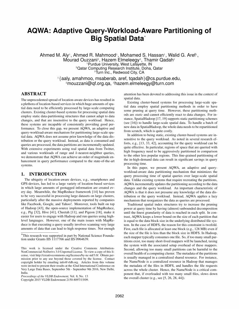
Figure 1: An overview of AQWA.
Theoretically, the number of possible partitioning layouts is ex-ponential in the total number of points because a partition can takeany shape and can contain any subset of the points. For simplicity,we consider only partitioning layouts that have rectangular-shapedpartitions. Moreover, to abide by the restrictions of typical dis-tributed file systems, e.g., HDFS, we consider only partitions thatare of size greater than a certain limit, e.g., the block size in HDFS.Our goal is to choose the cheapest partitioning layout according tothe above equation.
In AQWA, the query workload is not known in advance. As thequeries are processed, the query workload should be automaticallylearned, and the underlying data points should be partitioned ac-cordingly. Similarly, when the query workload changes, the datapartitions should be updated accordingly. Furthermore, as data up-dates are received, the data partitions need to be incrementally up-dated according to the distribution of the data and query workload.
3.2 Overview of AQWAFigure 1 gives an overview of AQWA that is composed of two
main components: 1) a k-d tree decomposition1 of the data, whereeach leaf node is a partition in the distributed file system, and 2) aset of main-memory structures that maintain statistics about the dis-tribution of the data and the queries. To account for system failures,the contents of the main-memory structures are periodically flushedinto disk. Upon recovery from a failure, the main-memory struc-tures are reloaded from disk. Four main processes define the inter-actions among the components of AQWA, namely, Initialization,Query Execution, Data Acquisition, and Repartitioning.
• Initialization: This process is performed once. Given an ini-tial dataset, statistics about the data distribution are collected.In particular, we divide the space into a grid, say G, of nrows and m columns. Each grid cell, say G[i, j], will con-tain the total number of points whose coordinates are insidethe boundaries of G[i, j]. The grid is kept in main-memoryand is used later on to find the number of points in a givenregion in O(1).
Based on the counts determined in the Initialization phase,we identify the best partitioning layout that evenly distributes
1The ideas presented in this paper do not assume a specific datastructure and are applicable to R-Tree or quadtree decomposition.
2064
the points in a kd-tree decomposition. We create the parti-tions using a MapReduce job that reads the entire data andassigns each data point to its corresponding partition. Wedescribe the initialization phase in detail in Section 4.1
• Query Execution: Given a query, we select the partitionsthat are relevant to, i.e., overlap, the invoked query. Then, theselected partitions are passed as input to a MapReduce job todetermine the actual data points that belong to the answer ofthe query. Afterwards, the query is logged into the same gridthat maintains the counts of points. After this update, wemay (or may not) take a decision to repartition the data.
• Data Acquisition: Given a batch of data, we issue a MapRe-duce job that appends each new data point to its correspond-ing partition according to the current layout of the partitions.In addition, the counts of points in the grid are incrementedaccording to the corresponding counts in the given batch ofdata.
• Repartitioning: Based on the history of the query workloadas well as the distribution of the data, we determine the parti-tion(s) that, if altered (i.e., further decomposed), would resultinto better execution time of the queries.
While the Initialization and Query Execution processes can beimplemented in a straightforward way, the Data Acquisition andRepartitioning processes raise the following performance chal-lenges:
• Overhead of Rewriting: A batch of data is appended duringthe Data Acquisition process. To have good pruning powerat query time, some partitions need to be split. Furthermore,the overall distribution of the data may change. Thus, wemay need to change the partitioning of the data. If the pro-cess of altering the partitioning layout reconstructs the par-titions from scratch, it would be very inefficient because itwill have to reread and rewrite the entire data. In Section 7,we show that reconstructing the partitions takes several hoursfor a few Terabytes of data. This is inefficient especially fordynamic scenarios, where new batches of data are appendedon an hourly or daily basis. Hence, we propose an incremen-tal mechanism to alter only a minimal number of partitionsaccording to the query workload.
• Efficient Search: We repeatedly search for the best change todo in the partitioning in order to achieve good query perfor-mance. The search space is large, and hence, we need an ef-ficient way to determine the partitions to be further split andhow/where the split should take place. We maintain main-memory aggregates about the distribution of the data and thequery workload. AQWA employs the techniques in [25, 8]to efficiently determine the partitioning decisions via main-memory lookups.
• Workload Changes and Time-Fading Weights: AQWAshould respond to permanent changes in the query workload.However, we need to ensure that AQWA is resilient to tempo-rary query workloads, i.e., avoid unnecessary repartitioningof the data.
AQWA keeps the history of all queries that have been pro-cessed. However, we need to differentiate between freshqueries, i.e., those that belong to the current query-workload,and relatively old queries. AQWA should alleviate the redun-dant repartitioning overhead corresponding to older query-workloads. Hence, we apply time-fading weights for the
/ 79
k-d Tree Variant
19x
y
Split one cell at a time
Stop when there are k partitions
1
2
3
4
5
6A
B
C
D
E
F G
(a)/ 79
k-d Tree Variant
19
1
2
D A
B C
F G
E
3
5
4
6
(b)
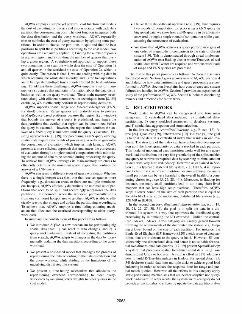
Figure 2: An example tree with 7 leaf partitions.
queries in order to alleviate the cost corresponding to oldqueries according to Equation 1.
• Keeping a lower bound on the size of each partition: Forpractical considerations, it is important to avoid small parti-tions that can introduce a performance bottleneck in a dis-tributed file system (e.g., see [5, 26, 28, 44]). Hence, inAQWA, we avoid splitting a partition if any of the result-ing two partitions is of size less than the block size in thedistributed file system (e.g., 128 MB in HDFS).
4. AQWA
4.1 InitializationThe main goal of AQWA is to partition the data in a way that
minimizes the cost according to Equation 1. Initially, i.e., beforeany query is executed, the number of queries that will overlap eachpartition is unknown. Hence, we simply assume a uniform distri-bution of the queries across the data. This implies that the onlycomponent of Equation 1 that matters at this initial stage is thenumber of points in each partition. Thus, in the Initialization pro-cess, we partition the data in a way that balances the number ofpoints across the partitions. In particular, we apply a recursive k-dtree decomposition [9].
The k-d tree is a binary tree in which every non-leaf node tries tosplit the underlying space into two parts that have the same num-ber of points. Only leaf nodes contain the actual data points. Thesplits can be horizontal or vertical and are chosen to balance thenumber of points across the leaf nodes. Splitting is recursively ap-plied, and stops if any of the resulting partitions is of size < theblock size. Figure 2 gives the initial state of an example k-d treewith 7 leaf nodes along with the corresponding space partitions.Once the boundaries of each leaf node are determined, a MapRe-duce job creates the initial partitions, i.e., assigns each data point toits corresponding partition. In this MapReduce job, for each point,say p, the key is the leaf node that encloses p, and the value is p.The mappers read different chunks of the data and then send eachpoint to the appropriate reducer, which groups the points that be-long to the same partition, and ultimately writes the correspondingpartition file into HDFS.
The hierarchy of the partitioning layout, i.e., the k-d tree, is keptfor processing future queries. As explained in Section 3.2, once aquery, say q, is received, only the leaf nodes of the tree that overlapq are selected and passed as input to the MapReduce job corre-sponding to q.
2065
/ 79
Number of points in p
38
Sum
Verti
cal A
ggre
gatio
n
Horizontal Aggregation
(a) Sum after aggregation. / 79
Number of points in p
44
+
+
–
–
O(1)
(b) O(1) lookups.
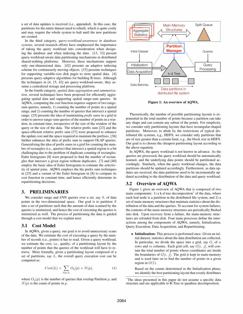
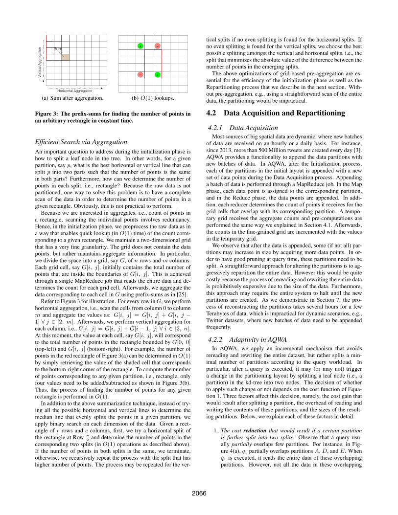
Figure 3: The prefix-sums for finding the number of points inan arbitrary rectangle in constant time.
Efficient Search via AggregationAn important question to address during the initialization phase ishow to split a leaf node in the tree. In other words, for a givenpartition, say p, what is the best horizontal or vertical line that cansplit p into two parts such that the number of points is the samein both parts? Furthermore, how can we determine the number ofpoints in each split, i.e., rectangle? Because the raw data is notpartitioned, one way to solve this problem is to have a completescan of the data in order to determine the number of points in agiven rectangle. Obviously, this is not practical to perform.
Because we are interested in aggregates, i.e., count of points ina rectangle, scanning the individual points involves redundancy.Hence, in the initialization phase, we preprocess the raw data as ina way that enables quick lookup (in O(1) time) of the count corre-sponding to a given rectangle. We maintain a two-dimensional gridthat has a very fine granularity. The grid does not contain the datapoints, but rather maintains aggregate information. In particular,we divide the space into a grid, say G, of n rows and m columns.Each grid cell, say G[i, j], initially contains the total number ofpoints that are inside the boundaries of G[i, j]. This is achievedthrough a single MapReduce job that reads the entire data and de-termines the count for each grid cell. Afterwards, we aggregate thedata corresponding to each cell in G using prefix-sums as in [25].
Refer to Figure 3 for illustration. For every row in G, we performhorizontal aggregation, i.e., scan the cells from column 0 to columnm and aggregate the values as: G[i, j] = G[i, j] + G[i, j −1] ∀ j ∈ [2, m]. Afterwards, we perform vertical aggregation foreach column, i.e., G[i, j] = G[i, j] + G[i − 1, j] ∀ i ∈ [2, n].At this moment, the value at each cell, say G[i, j], will correspondto the total number of points in the rectangle bounded by G[0, 0](top-left) and G[i, j] (bottom-right). For example, the number ofpoints in the red rectangle of Figure 3(a) can be determined in O(1)by simply retrieving the value of the shaded cell that correspondsto the bottom-right corner of the rectangle. To compute the numberof points corresponding to any given partition, i.e., rectangle, onlyfour values need to be added/subtracted as shown in Figure 3(b).Thus, the process of finding the number of points for any givenrectangle is performed in O(1).
In addition to the above summarization technique, instead of try-ing all the possible horizontal and vertical lines to determine themedian line that evenly splits the points in a given partition, weapply binary search on each dimension of the data. Given a rect-angle of r rows and c columns, first, we try a horizontal split ofthe rectangle at Row r
2and determine the number of points in the
corresponding two splits (in O(1) operations as described above).If the number of points in both splits is the same, we terminate,otherwise, we recursively repeat the process with the split that hashigher number of points. The process may be repeated for the ver-
tical splits if no even splitting is found for the horizontal splits. Ifno even splitting is found for the vertical splits, we choose the bestpossible splitting amongst the vertical and horizontal splits, i.e., thesplit that minimizes the absolute value of the difference between thenumber of points in the emerging splits.
The above optimizations of grid-based pre-aggregation are es-sential for the efficiency of the initialization phase as well as theRepartitioning process that we describe in the next section. With-out pre-aggregation, e.g., using a straightforward scan of the entiredata, the partitioning would be impractical.
4.2 Data Acquisition and Repartitioning
4.2.1 Data AcquisitionMost sources of big spatial data are dynamic, where new batches
of data are received on an hourly or a daily basis. For instance,since 2013, more than 500 Million tweets are created every day [3].AQWA provides a functionality to append the data partitions withnew batches of data. In AQWA, after the Initialization process,each of the partitions in the initial layout is appended with a newset of data points during the Data Acquisition process. Appendinga batch of data is performed through a MapReduce job. In the Mapphase, each data point is assigned to the corresponding partition,and in the Reduce phase, the data points are appended. In addi-tion, each reducer determines the count of points it receives for thegrid cells that overlap with its corresponding partition. A tempo-rary grid receives the aggregate counts and pre-computations areperformed the same way we explained in Section 4.1. Afterwards,the counts in the fine-grained grid are incremented with the valuesin the temporary grid.
We observe that after the data is appended, some (if not all) par-titions may increase in size by acquiring more data points. In or-der to have good pruning at query time, these partitions need to besplit. A straightforward approach for altering the partitions is to ag-gressively repartition the entire data. However this would be quitecostly because the process of rereading and rewriting the entire datais prohibitively expensive due to the size of the data. Furthermore,this approach may require the entire system to halt until the newpartitions are created. As we demonstrate in Section 7, the pro-cess of reconstructing the partitions takes several hours for a fewTerabytes of data, which is impractical for dynamic scenarios, e.g.,Twitter datasets, where new batches of data need to be appendedfrequently.
4.2.2 Adaptivity in AQWAIn AQWA, we apply an incremental mechanism that avoids
rereading and rewriting the entire dataset, but rather splits a min-imal number of partitions according to the query workload. Inparticular, after a query is executed, it may (or may not) triggera change in the partitioning layout by splitting a leaf node (i.e., apartition) in the kd-tree into two nodes. The decision of whetherto apply such change or not depends on the cost function of Equa-tion 1. Three factors affect this decision, namely, the cost gain thatwould result after splitting a partition, the overhead of reading andwriting the contents of these partitions, and the sizes of the result-ing partitions. Below, we explain each of these factors in detail.
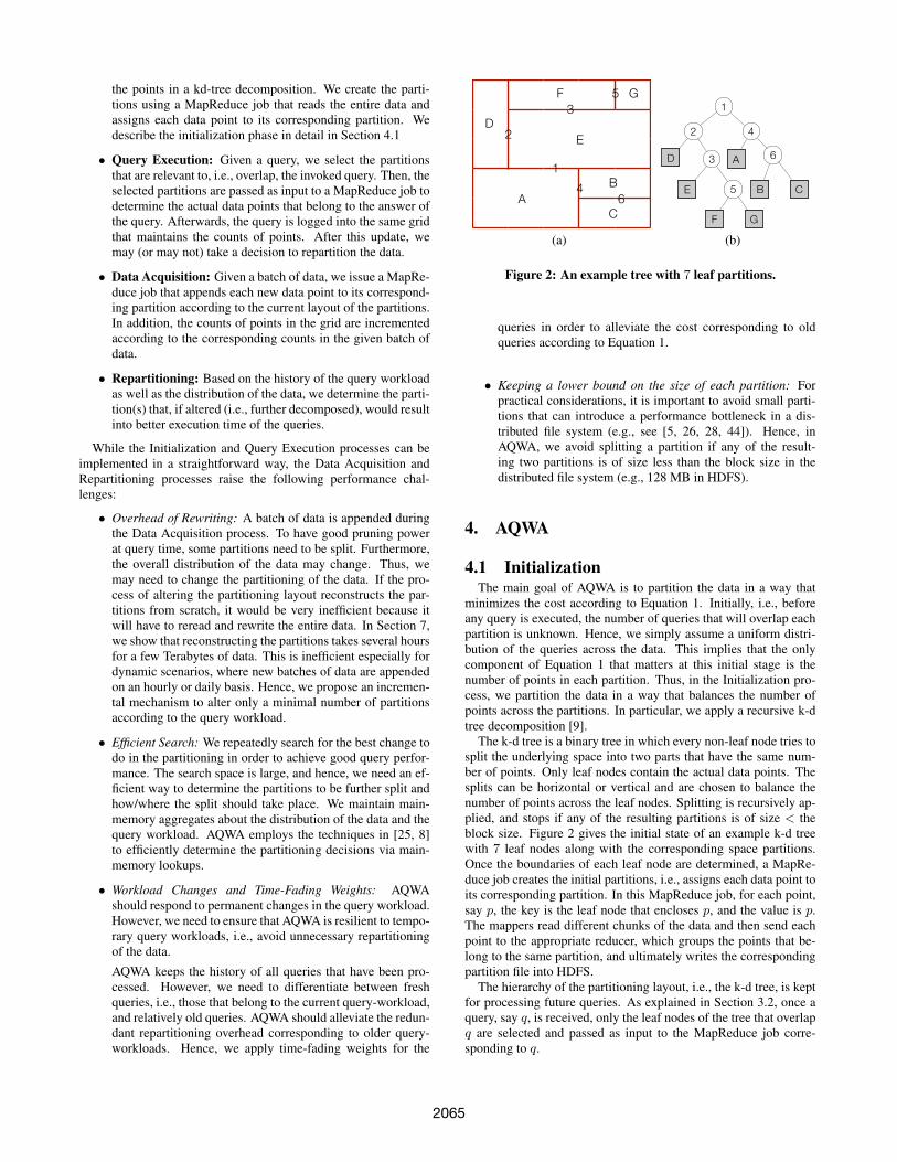
1. The cost reduction that would result if a certain partitionis further split into two splits: Observe that a query usu-ally partially overlaps few partitions. For instance, in Fig-ure 4(a), q1 partially overlaps partitions A, D, and E. Whenq1 is executed, it reads the entire data of these overlappingpartitions. However, not all the data in these overlapping
2066
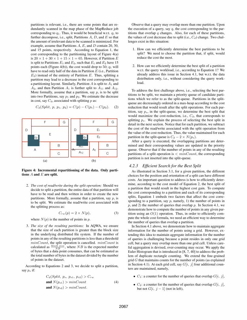
partitions is relevant, i.e., there are some points that are re-dundantly scanned in the map phase of the MapReduce jobcorresponding to q1. Thus, it would be beneficial w.r.t. q1 tofurther decompose, i.e., split, Partitions A, D, and E so thatthe amount of irrelevant data to be scanned is minimized. Forexample, assume that Partitions A, E, and D contain 20, 30,and 15 points, respectively. According to Equation 1, thecost corresponding to the partitioning layout of Figure 4(a)is 20× 1 + 30× 1 + 15× 1 = 65. However, if Partition Eis split to Partitions E1 and E2, such that E1 and E2 have 15points each (Figure 4(b)), the cost would drop to 50; q1 willhave to read only half of the data in Partition E (i.e., PartitionE2) instead of the entirety of Partition E. Thus, splitting apartition may lead to a decrease in the cost corresponding toa partitioning layout. Similarly, Partition A is split to A1 andA2, and then Partition A1 is further split to A11 and A12.More formally, assume that a partition, say p, is to be splitinto two Partitions, say p1 and p2. We estimate the decreasein cost, say Cd, associated with splitting p as:
Cd(Split, p, p1, p2) = C(p)− C(p1)− C(p2). (2)
/ 79
k-d Tree Variant
20x
y
Split one cell at a time
Stop when there are k partitions
A
B
C
D
E
F G
q1
(a) / 79
k-d Tree Variant
4x
y
Split one cell at a time
Stop when there are k partitions
D E1
F G
q1 E2
B
CA1 A2
A11
A12
(b)
Figure 4: Incremental repartitioning of the data. Only parti-tions A and E are split.
2. The cost of read/write during the split operation: Should wedecide to split a partition, the entire data of that partition willhave to be read and then written in order to create the newpartitions. More formally, assume that a partition, say p, isto be split. We estimate the read/write cost associated withthe splitting process as:
Crw(p) = 2×N(p), (3)
where N(p) is the number of points in p.
3. The size of the resulting partitions: In AQWA, we ensurethat the size of each partition is greater than the block sizein the underlying distributed file system. If the number ofpoints in any of the resulting partitions is less than a thresholdminCount, the split operation is cancelled. minCount iscalculated as block size
NB, where NB is the expected number
of bytes that a data point consumes, that can be estimated asthe total number of bytes in the dataset divided by the numberof points in the dataset.
According to Equations 2 and 3, we decide to split a partition,say ps if:
Cd(Split, ps, ps1, ps2) > Crw
and N(ps1) > minCount (4)and N(ps2) > minCount.
Observe that a query may overlap more than one partition. Uponthe execution of a query, say q, the cost corresponding to the par-titions that overlap q changes. Also, for each of these partitions,the values of cost decrease due to split (i.e., Cd) change. Two chal-lenges exist in this situation:
1. How can we efficiently determine the best partitions to besplit? We need to choose the partition that, if split, wouldreduce the cost the most.
2. How can we efficiently determine the best split of a partitionw.r.t. the query workload, i.e., according to Equation 1? Wealready address this issue in Section 4.1, but w.r.t. the datadistribution only, i.e., without considering the query work-load.
To address the first challenge above, i.e., selecting the best par-titions to be split, we maintain a priority queue of candidate parti-tions which we refer to as the split-queue. Partitions in the split-queue are decreasingly ordered in a max-heap according to the costreduction that would result after the split operations. For each par-tition, say ps, in the split-queue, we determine the best split thatwould maximize the cost-reduction, i.e., Cd, that corresponds tosplitting ps. We explain the process of selecting the best split indetail in the next section. Notice that for each partition, we subtractthe cost of the read/write associated with the split operation fromthe value of the cost-reduction. Thus, the value maintained for eachpartition in the split-queue is Cd − 2×N(ps).
After a query is executed, the overlapping partitions are deter-mined and their corresponding values are updated in the priorityqueue. Observe that if the number of points in any of the resultingpartitions of a split operation is < minCount, the correspondingpartition is not inserted into the split-queue.
4.2.3 Efficient Search for the Best SplitAs illustrated in Section 3.1, for a given partition, the different
choices for the position and orientation of a split can have differentcosts. An important question to address is how to efficiently deter-mine, according to the cost model of Equation 2, the best split ofa partition that would result in the highest cost gain. To computethe cost corresponding to a partition and each of its correspondingsplits, Equation 1 embeds two factors that affect the cost corre-sponding to a partition, say p, namely, 1) the number of points inp, and 2) the number of queries that overlap p. In Section 4.1, wedemonstrate how to compute the number of points in any given par-tition using an O(1) operation. Thus, in order to efficiently com-pute the whole cost formula, we need an efficient way to determinethe number of queries that overlap a partition.
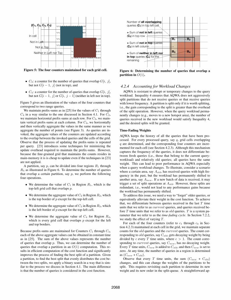
In Section 4.1 above, we demonstrate how to maintain aggregateinformation for the number of points using a grid. However, ex-tending this idea to maintain aggregate information for the numberof queries is challenging because a point resides in only one gridcell, but a query may overlap more than one grid cell. Unless care-ful aggregation is devised, over-counting may occur. We apply theEuler Histogram that is introduced in [8, 7, 40] to address the prob-lem of duplicate rectangle counting. We extend the fine-grainedgrid G that maintains counts for the number of points (as explainedin Section 4.1). At each grid cell, say G[i, j] four additional coun-ters are maintained, namely,
• C1: a counter for the number of queries that overlap G[i, j],
• C2: a counter for the number of queries that overlap G[i, j],but not G[i, j − 1] (not in left),
2067
/ 79
Number of regions Overlapping with p Inserting a region
66
1, 1, 1, 1 1, 0, 1, 0 1, 0, 1, 0 1, 0, 1, 0
1, 1, 0, 0 1, 0, 0, 0 1, 0, 0, 0 1, 0, 0, 0
1, 1, 0, 0 1, 0, 0, 0 2, 1, 1, 1 2, 0, 1, 0 1, 0, 1, 0 1, 0, 1, 0
1, 1, 0, 0 1, 0, 0, 0 2, 1, 0, 0 2, 0, 0, 0 1, 0, 0, 0 1, 0, 0, 0
1, 1, 0, 0 1, 0, 0, 0 1, 0, 0, 0 1, 0, 0, 0
1, 1, 0, 0 1, 0, 0, 0 1, 0, 0, 0 1, 0, 0, 0
(C1, C2, C3, C4)
In cell
Not in Left
Not in Top
Neither in Left nor Top
Figure 5: The four counters maintained for each grid cell.
• C3: a counter for the number of queries that overlap G[i, j],but not G[i− 1, j] (not in top), and
• C4: a counter for the number of queries that overlap G[i, j],but not G[i− 1, j] or G[i, j − 1] (neither in left nor in top).
Figure 5 gives an illustration of the values of the four counters thatcorrespond to two range queries.
We maintain prefix-sums as in [25] for the values of C1 throughC4 in a way similar to the one discussed in Section 4.1. For C2,we maintain horizontal prefix-sums at each row. For C3, we main-tain vertical prefix-sums at each column. For C4, we horizontallyand then vertically aggregate the values in the same manner as weaggregate the number of points (see Figure 3). As queries are in-voked, the aggregate values of the counters are updated accordingto the overlap between the invoked queries and the cells of the grid.Observe that the process of updating the prefix-sums is repeatedper query. [23] introduces some techniques for minimizing theupdate overhead required to maintain the prefix-sums. However,because the fine-grained grid that maintains the counts resides inmain-memory it is is cheap to update even if the techniques in [23]are not applied.
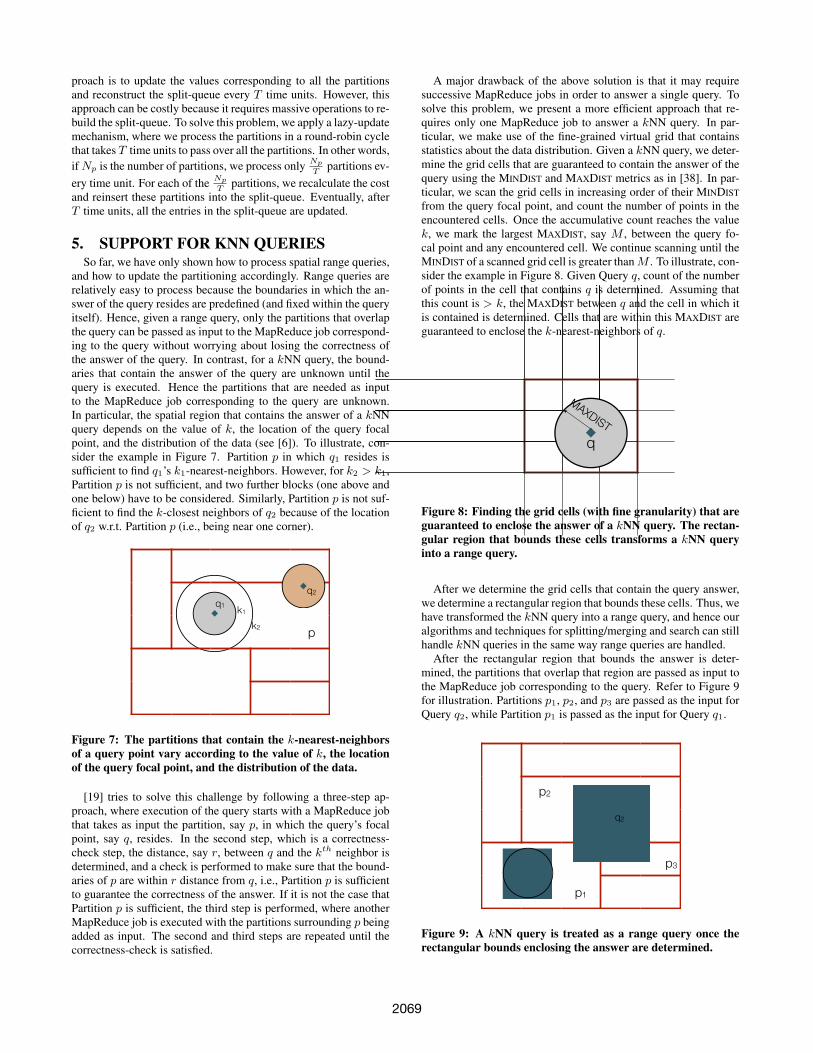
A partition, say p, can be divided into four regions R1 throughR4 as illustrated in Figure 6. To determine the number of queriesthat overlap a certain partition, say p, we perform the followingfour operations.
• We determine the value of C1 in Region R1, which is thetop-left grid cell that overlaps p.
• We determine the aggregate value of C2 in Region R2, whichis the top border of p except for the top-left cell.
• We determine the aggregate value of C3 in Region R3, whichis the left border of p except for the top-left cell.
• We determine the aggregate value of C4 for Region R4,which is every grid cell that overlaps p except for the leftand top borders.
Because prefix-sums are maintained for Counters C1 through C4,each of the above aggregate values can be obtained in constant timeas in [25]. The sum of the above values represents the numberof queries that overlap p. Thus, we can determine the number ofqueries that overlap a partition in an O(1) computation. This re-sults in efficient computation of the cost function and significantlyimproves the process of finding the best split of a partition. Givena partition, to find the best split that evenly distributes the cost be-tween the two splits, we apply a binary search in a way that is sim-ilar to the process we discuss in Section 4.1. The main differenceis that the number of queries is considered in the cost function.
/ 79
Finding the Number of Regions Overlapping with p
55
R1 R2
R3 R4
Number of all overlapping queries (C1) in top left cell
+ Sum of not in left queries (C2) in top row
+ Sum of not in top queries (C3) in left column
+ Sum of neither in left nor in top queries (C4) for the remaining
Figure 6: Determining the number of queries that overlap apartition in O(1).
4.2.4 Accounting for Workload ChangesAQWA is resistant to abrupt or temporary changes to the query
workload. Inequality 4 ensures that AQWA does not aggressivelysplit partitions that do not receive queries or that receive querieswith lower frequency. A partition is split only if it is worth splitting,i.e., the gain corresponding to the split is greater than the overheadof the split operation. However, when the query workload perma-nently changes (e.g., moves to a new hotspot area), the number ofqueries received in the new workload would satisfy Inequality 4,and the desired splits will be granted.
Time-Fading WeightsAQWA keeps the history of all the queries that have been pro-cessed. For every processed query, say q, grid cells overlappingq are determined, and the corresponding four counters are incre-mented for each cell (see Section 4.2.3). Although this mechanismcaptures the frequency of the queries, it does not differentiate be-tween fresh queries (i.e., those that belong to the current query-workload) and relatively old queries; all queries have the sameweight. This can lead to poor performance in AQWA especiallywhen a query workload changes. To illustrate, consider a scenariowhere a certain area, say Aold, has received queries with high fre-quency in the past, but the workload has permanently shifted toanother area, say Anew. If a new batch of data is received, it maytrigger a set of split operations at Aold. However, these splits areredundant, i.e., would not lead to any performance gains becausethe workload has permanently shifted.
To address this issue, we need a way to “forget” older queries, orequivalently alleviate their weight in the cost function. To achievethat, we differentiate between queries received in the last T timeunits that we refer to as current queries, and queries received be-fore T time units that we refer to as old queries. T is a system pa-rameter that we refer to as the time-fading cycle. In Section 7.2.2,we study the effect of varying T .
For each of the four counters (refer to c1 through c4 in Sec-tion 4.2.3) maintained at each cell in the grid, we maintain separatecounts for the old queries and the current queries. The count cor-responding to old queries, say Cold, gets decaying weight by beingdivided by c every T time units, where c > 1. The count corre-sponding to current queries, say Cnew, has no decaying weight.Every T time units, Cnew is added to Cold, and then Cnew is set tozero. At any time, the number of queries in a region is determinedas (Cnew + Cold).
Observe that every T time units, the sum (Cnew + Cold)changes, and this can change the weights of the partitions to besplit. This requires revisiting each partition to determine its newweight and its new order in the split-queue. A straightforward ap-
2068
proach is to update the values corresponding to all the partitionsand reconstruct the split-queue every T time units. However, thisapproach can be costly because it requires massive operations to re-build the split-queue. To solve this problem, we apply a lazy-updatemechanism, where we process the partitions in a round-robin cyclethat takes T time units to pass over all the partitions. In other words,if Np is the number of partitions, we process only Np
Tpartitions ev-
ery time unit. For each of the Np
Tpartitions, we recalculate the cost
and reinsert these partitions into the split-queue. Eventually, afterT time units, all the entries in the split-queue are updated.
5. SUPPORT FOR KNN QUERIESSo far, we have only shown how to process spatial range queries,
and how to update the partitioning accordingly. Range queries arerelatively easy to process because the boundaries in which the an-swer of the query resides are predefined (and fixed within the queryitself). Hence, given a range query, only the partitions that overlapthe query can be passed as input to the MapReduce job correspond-ing to the query without worrying about losing the correctness ofthe answer of the query. In contrast, for a kNN query, the bound-aries that contain the answer of the query are unknown until thequery is executed. Hence the partitions that are needed as inputto the MapReduce job corresponding to the query are unknown.In particular, the spatial region that contains the answer of a kNNquery depends on the value of k, the location of the query focalpoint, and the distribution of the data (see [6]). To illustrate, con-sider the example in Figure 7. Partition p in which q1 resides issufficient to find q1’s k1-nearest-neighbors. However, for k2 > k1,Partition p is not sufficient, and two further blocks (one above andone below) have to be considered. Similarly, Partition p is not suf-ficient to find the k-closest neighbors of q2 because of the locationof q2 w.r.t. Partition p (i.e., being near one corner).
/ 796
AQWA - Support for kNN Queries
k1
k2
q1
q2
p
Figure 7: The partitions that contain the k-nearest-neighborsof a query point vary according to the value of k, the locationof the query focal point, and the distribution of the data.
[19] tries to solve this challenge by following a three-step ap-proach, where execution of the query starts with a MapReduce jobthat takes as input the partition, say p, in which the query’s focalpoint, say q, resides. In the second step, which is a correctness-check step, the distance, say r, between q and the kth neighbor isdetermined, and a check is performed to make sure that the bound-aries of p are within r distance from q, i.e., Partition p is sufficientto guarantee the correctness of the answer. If it is not the case thatPartition p is sufficient, the third step is performed, where anotherMapReduce job is executed with the partitions surrounding p beingadded as input. The second and third steps are repeated until thecorrectness-check is satisfied.
A major drawback of the above solution is that it may requiresuccessive MapReduce jobs in order to answer a single query. Tosolve this problem, we present a more efficient approach that re-quires only one MapReduce job to answer a kNN query. In par-ticular, we make use of the fine-grained virtual grid that containsstatistics about the data distribution. Given a kNN query, we deter-mine the grid cells that are guaranteed to contain the answer of thequery using the MINDIST and MAXDIST metrics as in [38]. In par-ticular, we scan the grid cells in increasing order of their MINDISTfrom the query focal point, and count the number of points in theencountered cells. Once the accumulative count reaches the valuek, we mark the largest MAXDIST, say M , between the query fo-cal point and any encountered cell. We continue scanning until theMINDIST of a scanned grid cell is greater than M . To illustrate, con-sider the example in Figure 8. Given Query q, count of the numberof points in the cell that contains q is determined. Assuming thatthis count is > k, the MAXDIST between q and the cell in which itis contained is determined. Cells that are within this MAXDIST areguaranteed to enclose the k-nearest-neighbors of q.
/ 79
AQWA - Support for kNN Queries
8
MINDISTScan &
Counting
MAXDIST
q
Figure 8: Finding the grid cells (with fine granularity) that areguaranteed to enclose the answer of a kNN query. The rectan-gular region that bounds these cells transforms a kNN queryinto a range query.
After we determine the grid cells that contain the query answer,we determine a rectangular region that bounds these cells. Thus, wehave transformed the kNN query into a range query, and hence ouralgorithms and techniques for splitting/merging and search can stillhandle kNN queries in the same way range queries are handled.
After the rectangular region that bounds the answer is deter-mined, the partitions that overlap that region are passed as input tothe MapReduce job corresponding to the query. Refer to Figure 9for illustration. Partitions p1, p2, and p3 are passed as the input forQuery q2, while Partition p1 is passed as the input for Query q1.
/ 799
AQWA - Support for kNN Queries
It’s not a map-only jobCan we ignore communication cost?
q1
q2
p2
p1
p3
Figure 9: A kNN query is treated as a range query once therectangular bounds enclosing the answer are determined.
2069
Observe that the process of determining the region that enclosesthe k-nearest-neighbors of a query point is efficient. The reasonis that the whole process is based on counting of main-memoryaggregates without any need to scan any data points. Moreover,because the granularity of the grid is fine, the determined regionis compact, and hence few partitions will be scanned during theexecution of the kNN query, which leads to high query throughput.
6. SYSTEM INTEGRITY
6.1 Concurrency ControlAs queries are received by AQWA, some partitions may need
to be altered. It is possible that while a partition is being split, anew query is received that may also trigger another split to the verysame partitions being altered. Unless an appropriate concurrencycontrol protocol is used, inconsistent partitioning will occur.
To address the above issue, we use a simple locking mechanismto coordinate the incremental updates of the partitions. In particu-lar, whenever a query, say q, triggers a split, before the partitionsare updated, q tries to acquire a lock on each of the partitions to bealtered. If q succeeds to acquire all the locks, i.e., no other queryhas a conflicting lock, then q is allowed to alter the partitions. Thelocks are released after the partitions are completely altered. If qcannot acquire the locks due to a concurrent query that already hasone or more locks on the partitions being altered, then the decisionto alter the partitions is cancelled. Observe that canceling such de-cision may negatively affect the quality of the partitioning, but onlytemporarily because for a given query workload, queries similar toq will keep arriving afterwards and the repartitioning will eventu-ally take place.
A similar concurrency issue arises when updating the split-queue. Because the split-queue resides in main-memory, updatingthe entries of queue is relatively fast (requires a few milliseconds).Hence, to avoid the case where two queries result in conflictingqueue updates, we serialize the process of updating the split-queueusing a critical section.
6.2 Fault ToleranceIn case of system failures, the information in the main-memory
structures might get lost which can affect the correctness of thequery evaluation and the accuracy of the cost computations corre-sponding to Equation 1.
The main-memory grid contains two types of counts: 1) countsfor the number of points, and 2) counts for the number of queries.When a new batch of data is received by AQWA, the counts ofthe number of points in the new batch are determined through aMapReduce job that automatically writes these counts into HDFS.Observe that the data points in the new batch are appended throughthe same MapReduce job. At this moment, the counts (of the num-ber of points) in the grid are incremented and flushed into disk.Hence, the counts of the number of points are always accurate evenif failures occur. Thus, the kNN queries are always answered cor-rectly.
As mentioned in Section 3.2, the counts corresponding to thequeries (i.e., rectangles) are periodically flushed to disk. Observethat: 1) the correctness of query evaluation does not depend onthese counts, and 2) only the accuracy of the computation of thecost function is affected by these counts, which, in the worst case,leads to a delayed decision of repartitioning. In the event of failurebefore the counts are flushed into disk and if the query workloadis consistently received at a certain spatial region, the counts ofqueries will be incremented and repartitioning will eventually oc-cur.
7. EXPERIMENTSIn this section, we evaluate the performance of AQWA. We re-
alized a cluster-based testbed in which we implemented AQWA aswell as static grid-based partitioning and static k-d tree partitioning(as in [19, 16]).2 We choose the k-d and grid-based partitioning asour baselines because this allows us to contrast AQWA against twodifferent extreme partitioning schemes: 1) pure spatial decompo-sition, i.e., when using a uniform grid, and 2) data decomposition,i.e., when using a k-d tree.
Experiments are conducted on a 7-node cluster runningHadoop 2.2 over Red Hat Enterprise Linux 6. Each node in thecluster is a Dell r720xd server that has 16 Intel E5-2650v2 cores,64 GB of memory, 48 B of local storage, and a 40 Gigabit Ethernetinterconnect. The number of cores in each node enables high paral-lelism across the whole cluster, i.e., we could easily run a MapRe-duce job with 7× 16 = 112 Map/Reduce tasks.
We use a real spatial dataset from Twitter. The tweets weregathered over a period of nearly 20 months (from January 2013to July 2014). Only the tweets that have spatial coordinates insidethe United States were considered. The number of tweets in thedataset is 1.5 Billion tweets comprising about 250 GB. The formatof each tweet is: tweet identifier, timestamp, longitude-latitude co-ordinates, and text. To better show the scalability of AQWA, wehave further replicated this data 10 times, reaching a scale of about2.5 Terabytes.
We virtually split the space according to a 1000× 1000 grid thatrepresents 1000 normalized unit-distance measures in each of thehorizontal and vertical dimensions. Because we are dealing withtweets in the United States, that has an area of 10 Million squarekilometers, each grid cell in our virtual partitioning covers nearly10 square kilometers, which is a fairly good splitting of the spacegiven the large scale of the data. The virtual grid represents thesearch space for the partitions as well as the count statistics that wemaintain.
7.1 InitializationData Size P Time Grid Time kd Time Grid (min) Time kd (min)
50 333 466.299592793 392.040467262 8E+00 6.53400779
100 666 912.102408876 707.658773818 2E+01 11.79431290
150 999 1,480.173519593 1,237.10215097 2E+01 20.61836918
200 1332 1,966.845743496 1,668.627141422 3E+01 27.81045236
250 1665 2,395.9295792312,008.021810296 4E+01 33.46703017
Time of Data Partitioning
Elap
sed
Tim
e (s
ec)
0
600
1200
1800
2400
3000
Data Size (GB)50 100 150 200 250
Static k-d treeStatic Grid
Time of Data Partitioning
Elap
sed
Tim
e (m
in)
0
8
16
24
32
40
Data Size (GB)50 100 150 200 250
Static k-d treeStatic Grid
Time of Data Partitioning
Elap
sed
Tim
e (m
in)
0
8
16
24
32
40
Data Size (GB)50 100 150 200 250
Static k-d treeStatic Grid
�1
(a) Small scale (up to 250 GB)
Data Size P Time Grid Time kd Time Grid (min) Time kd (min)
0.5 333 3,780.000000000 3,937.294230462 1E+00 1.09369284 4E+03
1 666 8,425.0000000007,786.810246857 2E+00 2.16300285
1.5 99913,076.791955398 11,427.413283981 4E+00 3.17428147
2 133217,966.845743496 15,427.413283981 5E+00 4.28539258
Time of Data Partitioning
Elap
sed
Tim
e (s
ec)
0
3600
7200
10800
14400
18000
Data Size (GB)0.5 1 1.5 2
Static k-d treeStatic Grid
Time of Data PartitioningEl
apse
d Ti
me
(hou
r)
0
1
2
3
4
5
Data Size (TB)0.5 1 1.5 2
Static k-d treeStatic Grid
Time of Data PartitioningEl
apse
d Ti
me
(hou
r)
0
1
2
3
4
5
Data Size (TB)0.5 1 1.5 2
Static k-d treeStatic Grid
�1
(b) Large scale (up to 2 TB)
Figure 10: Performance of the initialization process.
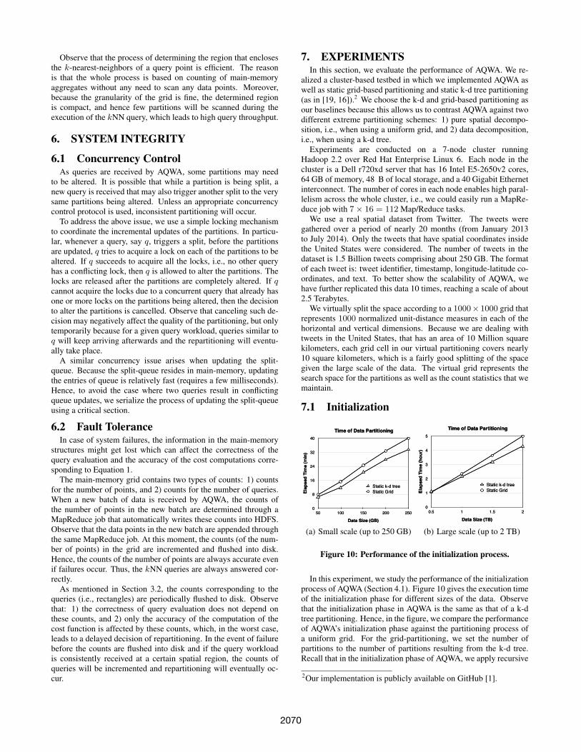
In this experiment, we study the performance of the initializationprocess of AQWA (Section 4.1). Figure 10 gives the execution timeof the initialization phase for different sizes of the data. Observethat the initialization phase in AQWA is the same as that of a k-dtree partitioning. Hence, in the figure, we compare the performanceof AQWA’s initialization phase against the partitioning process ofa uniform grid. For the grid-partitioning, we set the number ofpartitions to the number of partitions resulting from the k-d tree.Recall that in the initialization phase of AQWA, we apply recursive
2Our implementation is publicly available on GitHub [1].
2070
k-d partitioning, and we stop when splitting a partition would resultinto small partitions, i.e., of size less than the block size in HDFS.
We observe that grid-partitioning requires relatively high execu-tion time. Each reduce task handles the data of one partition. Dueto the skewness of the data distribution, the load across the reducetasks will be unbalanced, causing certain grid cells, i.e., partitions,to receive more data points than others. Because a MapReduce jobdoes not terminate until the last reduce task completes, the unbal-anced load leads to a relatively high execution time compared to thekd-tree. In contrast, the k-d tree partitioning, which is employed byAQWA, balances the data sizes across all the partitions.
We also observe that as the data size increases, the time requiredto perform the partitioning increases. As Figure 10(b) demon-strates, building the partitions from scratch for the whole data takesnearly five hours for only two Terabytes of data. Although thisis a natural result, it motivates AQWA’s incremental methodologyin repartitioning, which is to avoid repartitioning the whole datathroughout the system lifetime. In particular, after the initializa-tion phase, AQWA never reconstructs the partitions again if newbatches of data are received. In contrast, AQWA alters a minimalnumber of partitions according to the query workload and the datadistribution.
7.2 Adaptivity in AQWAIn the following experiments, we study the query performance in
AQWA. Our performance measures are: 1) the system throughput,which indicates the number of queries that can be answered per unittime, and 2) the split overhead, which indicates the time required toperform the split operations. To ensure full system utilization, weissue batches of queries that are submitted to the system at once.The number of queries per batch is 20. The throughput is calculatedby dividing 20 over the elapsed time to process the queries in abatch.
7.2.1 Data Acquisition andIncremental Repartitioning
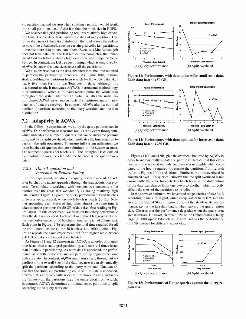
In this experiment, we study the query performance of AQWAafter batches of data are appended through the data acquisition pro-cess. To simulate a workload with hotspots, we concentrate thequeries over the areas that we identify as having relatively highdata density. Figure 11 gives the query performance when batchesof tweets are appended, where each batch is nearly 50 GB. Notethat appending each batch of data takes almost the same time ittakes to create partitions for 50 GB of data (i.e., first reading in Fig-ure 10(a)). In this experiment, we focus on the query performanceafter the data is appended. Each point in Figure 11(a) represents theaverage performance for 50 batches of queries (each of 20 queries).Each point in Figure 11(b) represents the total time required for allthe split operations for all the 50 batches, i.e., 1000 queries. Fig-ure 12 repeats the same experiment, but for a higher scale, where250 GB of data is appended at each batch.
As Figures 11 and 12 demonstrate, AQWA is an order of magni-tude faster than a static grid-partitioning, and nearly 4 times fasterthan a static k-d partitioning. As more data is appended, the perfor-mance of both the static grid and k-d partitioning degrades becauseboth are static. In contrast, AQWA maintains steady throughput re-gardless of the overall size of the data because it can dynamicallysplit the partitions according to the query workload. One can ar-gue that the static k-d partitioning could split as data is appended,however, this is quite costly because it requires reading and writ-ing (almost) all the partitions (i.e., the entire data) from scratch.In contrast, AQWA determines a minimal set of partitions to splitaccording to the query workload.
Data Size AQWA Static Grid Static k-d tree AQWA Static Grid Static k-d tree AQWA
1 26.000000000 10.658575425 3E+01 39.00708540 288 3E+01 8
2 2.000000000 7.042423459 3E+01 42.08974081 477 6E+01 7
3 5.000000000 5.598749792 2E+01 39.38929345 618 9E+01 10
4 4.000000000 4.209893897 2E+01 43.57126150 843 1E+02 10
5 15.000000000 3.400080053 2E+01 50.00367360 1,071 2E+02 9
6
7
8
9
10
Query Performance
Thro
ughp
ut (q
uery
/ m
in)
1
10
100
Timeline – Data Batch ID1 2 3 4 5
Query Performance
Thro
ughp
ut (q
uery
/ m
in)
1
10
100
Timeline – Data Batch ID1 2 3 4 5
Static k-d treeStatic GridAQWA
Total Time Across Mappers
Map
pers
Tim
e (s
ec)
1
10
100
1000
Timeline – Data Batch ID1 2 3 4 5
Total Time Across Mappers
1
10
100
1000
Timeline – Data Batch ID1 2 3 4 5
Static k-d treeStatic GridAQWA
Time of Split Operations
Tim
e (s
ec)
0
6
12
18
24
30
Timeline – Data Batch ID1 2 3 4 5
AQWA
�1
(a) Query performance
Data Size AQWA Static Grid Static k-d tree AQWA Static Grid Static k-d tree AQWA
1 26.000000000 10.658575425 3E+01 39.00708540 288 3E+01 8
2 2.000000000 7.042423459 3E+01 42.08974081 477 6E+01 7
3 5.000000000 5.598749792 2E+01 39.38929345 618 9E+01 10
4 4.000000000 4.209893897 2E+01 43.57126150 843 1E+02 10
5 15.000000000 3.400080053 2E+01 50.00367360 1,071 2E+02 9
6
7
8
9
10
Query Performance
Thro
ughp
ut (q
uery
/ m
in)
1
10
100
Timeline – Data Batch ID1 2 3 4 5
Query Performance
Thro
ughp
ut (q
uery
/ m
in)
1
10
100
Timeline – Data Batch ID1 2 3 4 5
Static k-d treeStatic GridAQWA
Total Time Across Mappers
Map
pers
Tim
e (s
ec)
1
10
100
1000
Timeline – Data Batch ID1 2 3 4 5
Total Time Across Mappers
1
10
100
1000
Timeline – Data Batch ID1 2 3 4 5
Static k-d treeStatic GridAQWA
Time of Split Operations
Tim
e (s
ec)
0
6
12
18
24
30
Timeline – Data Batch ID1 2 3 4 5
AQWA
Time of Split Operations
Tim
e (s
ec)
0
6
12
18
24
30
Timeline – Data Batch ID1 2 3 4 5
AQWA
�1
(b) Split overhead
Figure 11: Performance with data updates for small scale data.Each data batch is 50 GB.
Data Size AQWA Static Grid Static k-d tree AQWA Static Grid Static k-d tree AQWA
1 70.000000000 19.047619048 3E+01 50.88072081 83 2E+01 10
2 35.000000000 18.448375543 3E+01 50.88072081 120 3E+01 8
3 8.000000000 15.558821185 2E+01 50.00000000 178 5E+01 10
4 68.000000000 11.856555075 2E+01 50.00000000 251 6E+01 10
5 40.000000000 11.041809260 2E+01 50.00000000 317 7E+01 12
6 20.000000000 9.519388892 2E+01 50.00000000 371 8E+01 10
7 26.000000000 8.548855825 2E+01 50.00000000 452 1E+02 11
8 0.000000000 7.666186203 2E+01 50.00000000 514 1E+02 11
9 27.000000000 7.054660063 2E+01 50.00000000 579 1E+02 14
10 6.000000000 6.638127000 2E+01 50.00000000 643 1E+02 11
Query Performance
Thro
ughp
ut (q
uery
/ m
in)
1
10
100
Timeline – Data Batch ID1 2 3 4 5 6 7 8 9 10
Query Performance
Thro
ughp
ut (q
uery
/ m
in)
1
10
100
Timeline – Data Batch ID1 2 3 4 5 6 7 8 9 10
Static k-d treeStatic GridAQWA
Total Time Across Mappers
Map
pers
Tim
e (s
ec)
1
10
100
1000
Timeline – Data Batch ID1 2 3 4 5 6 7 8 9 10
Total Time Across Mappers
1
10
100
1000
Timeline – Data Batch ID1 2 3 4 5 6 7 8 9 10
Static k-d treeStatic GridAQWA
Time of Split Operations
Tim
e (s
ec)
0
14
28
42
56
70
Timeline – Data Batch ID1 2 3 4 5 6 7 8 9 10
AQWA
Time of Split Operations
Tim
e (s
ec)
0
14
28
42
56
70
Timeline – Data Batch ID1 2 3 4 5 6 7 8 9 10
AQWA
�1
(a) Query performance
Data Size AQWA Static Grid Static k-d tree AQWA Static Grid Static k-d tree AQWA
1 70.000000000 19.047619048 3E+01 50.88072081 83 2E+01 10
2 35.000000000 18.448375543 3E+01 50.88072081 120 3E+01 8
3 8.000000000 15.558821185 2E+01 50.00000000 178 5E+01 10
4 68.000000000 11.856555075 2E+01 50.00000000 251 6E+01 10
5 40.000000000 11.041809260 2E+01 50.00000000 317 7E+01 12
6 20.000000000 9.519388892 2E+01 50.00000000 371 8E+01 10
7 26.000000000 8.548855825 2E+01 50.00000000 452 1E+02 11
8 0.000000000 7.666186203 2E+01 50.00000000 514 1E+02 11
9 27.000000000 7.054660063 2E+01 50.00000000 579 1E+02 14
10 6.000000000 6.638127000 2E+01 50.00000000 643 1E+02 11
Query Performance
Thro
ughp
ut (q
uery
/ m
in)
1
10
100
Timeline – Data Batch ID1 2 3 4 5 6 7 8 9 10
Query Performance
Thro
ughp
ut (q
uery
/ m
in)
1
10
100
Timeline – Data Batch ID1 2 3 4 5 6 7 8 9 10
Static k-d treeStatic GridAQWA
Total Time Across Mappers
Map
pers
Tim
e (s
ec)
1
10
100
1000
Timeline – Data Batch ID1 2 3 4 5 6 7 8 9 10
Total Time Across Mappers
1
10
100
1000
Timeline – Data Batch ID1 2 3 4 5 6 7 8 9 10
Static k-d treeStatic GridAQWA
Time of Split Operations
Tim
e (s
ec)
0
14
28
42
56
70
Timeline – Data Batch ID1 2 3 4 5 6 7 8 9 10
AQWA
Time of Split Operations
Tim
e (s
ec)
0
14
28
42
56
70
Timeline – Data Batch ID1 2 3 4 5 6 7 8 9 10
AQWA
�1
(b) Split overhead
Figure 12: Performance with data updates for large scale data.Each data batch is 250 GB.
Figures 11(b) and 12(b) give the overhead incurred by AQWA inorder to incrementally update the partitions. Notice that this over-head is in the scale of seconds, and hence is negligible when com-pared to the hours required to recreate the partitions from scratch(refer to Figures 10(b) and 10(a)). Furthermore, this overhead isamortized over 1000 queries. Observe that the split overhead is notconsistently the same for each data batch because the distributionof the data can change from one batch to another, which directlyaffects the sizes of the partitions to be split.
In the above experiment, we have used range queries of size 5×5according to our virtual grid, which is equivalent to 0.0025% of thearea of the United States. Figure 13 gives the steady-state perfor-mance, i.e., at the last data batch, when varying the query regionsize. Observe that the performance degrades when the query areasize increases. However, an area of 1% of the United States is fairlylarge (10,000 square kilometers). Figure 14 gives the performanceof kNN queries for different values of k.
Data Size AQWA Static Grid Static k-d tree AQWA Static Grid Static k-d tree AQWA
0.0001% 49.000000000 7.027954981 2E+01 64.83555292 470 1E+02 8
0.01% 107.000000000 6.517609538 2E+01 38.82328506 515 1E+02 10
1% 1,373.000000000 3.000000000 2E+00 5.42923849 1,306 2E+03 649
49.000000000
Query Performance
Thro
ughp
ut (q
uery
/ m
in)
1
10
100
Query Area Size0.0001% 0.01% 1%
Query Performance
Thro
ughp
ut (q
uery
/ m
in)
1
10
100
0.0001% 0.01% 1%
Static k-d treeStatic GridAQWA
Total Time Across Mappers
Map
pers
Tim
e (s
ec)
1
10
100
1000
Query Area Size0.0001% 0.01% 1%
Total Time Across Mappers
1
10
100
1000
0.0001% 0.01% 1%
Static k-d treeStatic GridAQWA
Time of Split Operations
Tim
e (s
ec)
0
280
560
840
1120
1400
Query Area Size0.0001% 0.01% 1%
AQWA
�1
(a) Query performance
Data Size AQWA Static Grid Static k-d tree AQWA Static Grid Static k-d tree AQWA
0.0001% 49.000000000 7.027954981 2E+01 64.83555292 470 1E+02 8
0.01% 107.000000000 6.517609538 2E+01 38.82328506 515 1E+02 10
1% 1,373.000000000 3.000000000 2E+00 5.42923849 1,306 2E+03 649
49.000000000
Query Performance
Thro
ughp
ut (q
uery
/ m
in)
1
10
100
Query Area Size0.0001% 0.01% 1%
Query Performance
Thro
ughp
ut (q
uery
/ m
in)
1
10
100
0.0001% 0.01% 1%
Static k-d treeStatic GridAQWA
Total Time Across Mappers
Map
pers
Tim
e (s
ec)
1
10
100
1000
Query Area Size0.0001% 0.01% 1%
Total Time Across Mappers
1
10
100
1000
0.0001% 0.01% 1%
Static k-d treeStatic GridAQWA
Time of Split Operations
Tim
e (s
ec)
0
280
560
840
1120
1400
Query Area Size0.0001% 0.01% 1%
AQWA
Time of Split Operations
Tim
e (s
ec)
0
280
560
840
1120
1400
Query Area Size0.0001% 0.01% 1%
AQWA
�1
(b) Split overhead
Figure 13: Performance of Range queries against the query re-gion size.
2071
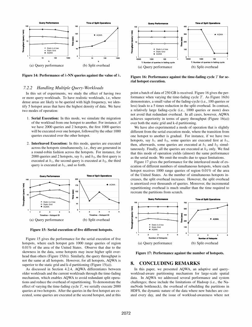
Data Size AQWA Static Grid Static k-d tree AQWA Static Grid Static k-d tree AQWA
1 45 6.000000000 20.000000000 60 647 153 11
10 54 6.401261322 19.838905550 61 555 128 10
100 80 7.000000000 18.844215342 59 557 125 9
1000 150 6.000000000 16.138934333 42 531 121 10
Query PerformanceTh
roug
hput
(que
ry /
min
)
1
10
100
k1 10 100 1000
Query PerformanceTh
roug
hput
(que
ry /
min
)
1
10
100
1 10 100 1000
Static k-d treeStatic GridAQWA
Total Time Across Mappers
Map
pers
Tim
e (s
ec)
1
10
100
1000
k1 10 100
Total Time Across Mappers
1
10
100
1000
1 10 100
Static k-d treeStatic GridAQWA
Time of Split Operations
Tim
e (s
ec)
0
40
80
120
160
k1 10 100 1000
AQWA
Time of Split Operations
Tim
e (s
ec)
0
40
80
120
160
1 10 100 1000
�1
(a) Query performance
Data Size AQWA Static Grid Static k-d tree AQWA Static Grid Static k-d tree AQWA
1 45 6.000000000 20.000000000 60 647 153 11
10 54 6.401261322 19.838905550 61 555 128 10
100 80 7.000000000 18.844215342 59 557 125 9
1000 150 6.000000000 16.138934333 42 531 121 10
Query Performance
Thro
ughp
ut (q
uery
/ m
in)
1
10
100
k1 10 100 1000
Query Performance
Thro
ughp
ut (q
uery
/ m
in)
1
10
100
1 10 100 1000
Static k-d treeStatic GridAQWA
Total Time Across Mappers
Map
pers
Tim
e (s
ec)
1
10
100
1000
k1 10 100
Total Time Across Mappers
1
10
100
1000
1 10 100
Static k-d treeStatic GridAQWA
Time of Split Operations
Tim
e (s
ec)
0
40
80
120
160
k1 10 100 1000
AQWA
Time of Split Operations
Tim
e (s
ec)
0
40
80
120
160
1 10 100 1000
�1
(b) Split overhead
Figure 14: Performance of k-NN queries against the value of k.
7.2.2 Handling Multiple QueryWorkloadsIn this set of experiments, we study the effect of having two
or more query-workloads. To have realistic workloads, i.e, wheredense areas are likely to be queried with high frequency, we iden-tify 5 hotspot areas that have the highest density of data. We havetwo modes of operation:
1. Serial Execution: In this mode, we simulate the migrationof the workload from one hotspot to another. For instance, ifwe have 2000 queries and 2 hotspots, the first 1000 querieswill be executed over one hotspot, followed by the other 1000queries executed over the other hotspot.
2. Interleaved Execution: In this mode, queries are executedacross the hotspots simultaneously, i.e., they are generated ina round-robin fashion across the hotspots. For instance, for2000 queries and 2 hotspots, say h1 and h2, the first query isexecuted at h1, the second query is executed at h2, the thirdquery is executed at h1, and so forth.
Data Size AQWA Static Grid Static k-d tree AQWA Static Grid Static k-d tree AQWA
1 204.000000000 6.339943498 1E+01 29.75904643 517 2E+02 18
2 64.000000000 11.036336981 2E+01 43.18497739 235 1E+02 8
3 127.000000000 6.512792643 2E+01 65.21541364 510 1E+02 9
4 75.000000000 5.943537482 2E+01 41.40377064 595 1E+02 9
5 50.000000000 3.391522199 1E+01 45.23692824 1,092 2E+02 8
Query Performance
Thro
ughp
ut (q
uery
/ m
in)
1
10
100
Timeline – Hotspot ID1 2 3 4 5
Query Performance
Thro
ughp
ut (q
uery
/ m
in)
1
10
100
1 2 3 4 5
Static k-d treeStatic GridAQWA
Total Time Across Mappers
Map
pers
Tim
e (s
ec)
1
10
100
1000
Timeline – Hotspot ID1 2 3 4 5
Total Time Across Mappers
1
10
100
1000
1 2 3 4 5
Static k-d treeStatic GridAQWA
Time of Split Operations
Tim
e (s
ec)
0
44
88
132
176
220
Timeline – Hotspot ID1 2 3 4 5
AQWA
Time of Split Operations
Tim
e (s
ec)
0
44
88
132
176
220
1 2 3 4 5
�1
(a) Query performance
Data Size AQWA Static Grid Static k-d tree AQWA Static Grid Static k-d tree AQWA
1 204.000000000 6.339943498 1E+01 29.75904643 517 2E+02 18
2 64.000000000 11.036336981 2E+01 43.18497739 235 1E+02 8
3 127.000000000 6.512792643 2E+01 65.21541364 510 1E+02 9
4 75.000000000 5.943537482 2E+01 41.40377064 595 1E+02 9
5 50.000000000 3.391522199 1E+01 45.23692824 1,092 2E+02 8
Query Performance
Thro
ughp
ut (q
uery
/ m
in)
1
10
100
Timeline – Hotspot ID1 2 3 4 5
Query Performance
Thro
ughp
ut (q
uery
/ m
in)
1
10
100
1 2 3 4 5
Static k-d treeStatic GridAQWA
Total Time Across Mappers
Map
pers
Tim
e (s
ec)
1
10
100
1000
Timeline – Hotspot ID1 2 3 4 5
Total Time Across Mappers
1
10
100
1000
1 2 3 4 5
Static k-d treeStatic GridAQWA
Time of Split Operations
Tim
e (s
ec)
0
44
88
132
176
220
Timeline – Hotspot ID1 2 3 4 5
AQWA
Time of Split Operations
Tim
e (s
ec)
0
44
88
132
176
220
1 2 3 4 5
�1
(b) Split overhead
Figure 15: Serial execution of five different hotspots.
Figure 15 gives the performance for the serial execution of fivehotspots, where each hotspot gets 1000 range queries of region0.01% of the area of the United States. Observe that due to theskewness in the data, some hotspots may incur higher split over-head than others (Figure 15(b)). Similarly, the query throughput isnot the same at all hotspots. However, for all hotspots, AQWA issuperior to the static grid and k-d partitioning (Figure 15(a)).
As discussed in Section 4.2.4, AQWA differentiates betweenolder workloads and the current workloads through the time-fadingmechanism, which enables AQWA to avoid redundant split opera-tions and reduce the overhead of repartitioning. To demonstrate theeffect of varying the time-fading cycle T , we serially execute 2000queries at two hotspots. After the queries in the first hotspot are ex-ecuted, some queries are executed at the second hotspot, and at this
Data Size AQWA Static Grid Static k-d tree AQWA Static Grid Static k-d tree AQWA
10000 360 7.760586806 20.928809735 52 416 98 8
1000 360 7.746923781 20.757992726 52 419 97 7
100 50 7.746761706 20.642338250 52 422 99 8
1 50 7.751963350 20.774527467 52 499 115 10
Query Performance
Thro
ughp
ut (q
uery
/ m
in)
1
10
100
T: Number of queries in fading cycle10000 1000 100 1
Query Performance
Thro
ughp
ut (q
uery
/ m
in)
1
10
100
10000 1000 100 1
Static k-d treeStatic GridAQWA
Total Time Across Mappers
Map
pers
Tim
e (s
ec)
1
10
100
1000
T: Number of queries in fading cycle10000 1000 100 1
Total Time Across Mappers
1
10
100
1000
10000 1000 100 1
Static k-d treeStatic GridAQWA
Time of Split Operations
Tim
e (s
ec)
0
100
200
300
400
T: Number of queries in fading cycle10000 1000 100 1
AQWA
Time of Split Operations
Tim
e (s
ec)
0
100
200
300
400
10000 1000 100 1
�1
(a) Query performance
Data Size AQWA Static Grid Static k-d tree AQWA Static Grid Static k-d tree AQWA
10000 360 7.760586806 20.928809735 52 416 98 8
1000 360 7.746923781 20.757992726 52 419 97 7
100 50 7.746761706 20.642338250 52 422 99 8
1 50 7.751963350 20.774527467 52 499 115 10
Query Performance
Thro
ughp
ut (q
uery
/ m
in)
1
10
100
T: Number of queries in fading cycle10000 1000 100 1
Query Performance
Thro
ughp
ut (q
uery
/ m
in)
1
10
100
10000 1000 100 1
Static k-d treeStatic GridAQWA
Total Time Across Mappers
Map
pers
Tim
e (s
ec)
1
10
100
1000
T: Number of queries in fading cycle10000 1000 100 1
Total Time Across Mappers
1
10
100
1000
10000 1000 100 1
Static k-d treeStatic GridAQWA
Time of Split Operations
Tim
e (s
ec)
0
100
200
300
400
T: Number of queries in fading cycle10000 1000 100 1
AQWA
Time of Split Operations
Tim
e (s
ec)
0
100
200
300
400
10000 1000 100 1
�1
(b) Split overhead
Figure 16: Performance against the time-fading cycle T for se-rial hotspot execution.
point a batch of data of 250 GB is received. Figure 16 gives the per-formance when varying the time-fading cycle T . As Figure 16(b)demonstrates, a small value of the fading-cycle (i.e., 100 queries orless) leads to a 5 times reduction in the split overhead. In contrast,a relatively large fading-cycle (i.e., 1000 queries or more) doesnot avoid that redundant overhead. In all cases, however, AQWAachieves superiority in terms of query throughput (Figure 16(a))over both the static grid and k-d partitioning.
We have also experimented a mode of operation that is slightlydifferent from the serial execution mode, where the transition fromone hotspot to another is gradual. For instance, if we have twohotspots, say h1 and h2, some queries are executed first at h1,then, afterwards, some queries are executed at h1 and h2 simul-taneously. Finally, all the queries are executed at h2 only. We findthat this mode of operation yields (almost) the same performanceas the serial mode. We omit the results due to space limitations.
Figure 17 gives the performance for the interleaved mode of ex-ecution of different numbers of simultaneous hotspots, where eachhotspot receives 1000 range queries of region 0.01% of the areaof the United States. As the number of simultaneous hotspots in-creases, the split overhead increases. However, the split overheadis amortized over thousands of queries. Moreover, the incrementalrepartitioning overhead is much smaller than the time required torecreate the partitions from scratch.
Data Size AQWA Static Grid Static k-d tree AQWA Static Grid Static k-d tree AQWA
1 234.000000000 5.915254504 2E+01 50.66098101 560 1E+02 11
2 525.000000000 8.556023925 2E+01 51.54517643 407 1E+02 10
3 550.000000000 8.087857556 2E+01 52.41612998 431 1E+02 10
4 577.000000000 7.235878758 2E+01 52.53919463 473 1E+02 8
5 642.000000000 5.914319370 2E+01 52.17391304 603 1E+02 10
Query Performance
Thro
ughp
ut (q
uery
/ m
in)
1
10
100
Number of Hotspots1 2 3 4 5
Query Performance
Thro
ughp
ut (q
uery
/ m
in)
1
10
100
1 2 3 4 5
Static k-d treeStatic GridAQWA
Total Time Across Mappers
Map
pers
Tim
e (s
ec)
1
10
100
1000
Number of Hotspots1 2 3 4 5
Total Time Across Mappers
1
10
100
1000
1 2 3 4 5
Static k-d treeStatic GridAQWA
Time of Split Operations
Tim
e (s
ec)
0
140
280
420
560
700
Number of Hotspots1 2 3 4 5
AQWA
�1
(a) Query performance
Data Size AQWA Static Grid Static k-d tree AQWA Static Grid Static k-d tree AQWA
1 234.000000000 5.915254504 2E+01 50.66098101 560 1E+02 11
2 525.000000000 8.556023925 2E+01 51.54517643 407 1E+02 10
3 550.000000000 8.087857556 2E+01 52.41612998 431 1E+02 10
4 577.000000000 7.235878758 2E+01 52.53919463 473 1E+02 8
5 642.000000000 5.914319370 2E+01 52.17391304 603 1E+02 10
Query Performance
Thro
ughp
ut (q
uery
/ m
in)
1
10
100
Number of Hotspots1 2 3 4 5
Query Performance
Thro
ughp
ut (q
uery
/ m
in)
1
10
100
1 2 3 4 5
Static k-d treeStatic GridAQWA
Total Time Across MappersM
appe
rs T
ime
(sec
)
1
10
100
1000
Number of Hotspots1 2 3 4 5
Total Time Across Mappers
1
10
100
1000
1 2 3 4 5
Static k-d treeStatic GridAQWA
Time of Split Operations
Tim
e (s
ec)
0
140
280
420
560
700
Number of Hotspots1 2 3 4 5
AQWA
Time of Split Operations
Tim
e (s
ec)
0
140
280
420
560
700
Number of Hotspots1 2 3 4 5
AQWA
�1
(b) Split overhead
Figure 17: Performance against the number of hotspots.
8. CONCLUDING REMARKSIn this paper, we presented AQWA, an adaptive and query-
workload-aware partitioning mechanism for large-scale spatialdata. In AQWA we addressed several performance and systemchallenges; these include the limitations of Hadoop (i.e., the Na-meNode bottleneck), the overhead of rebuilding the partitions inHDFS, the dynamic nature of the data where new batches are cre-ated every day, and the issue of workload-awareness where not
2072
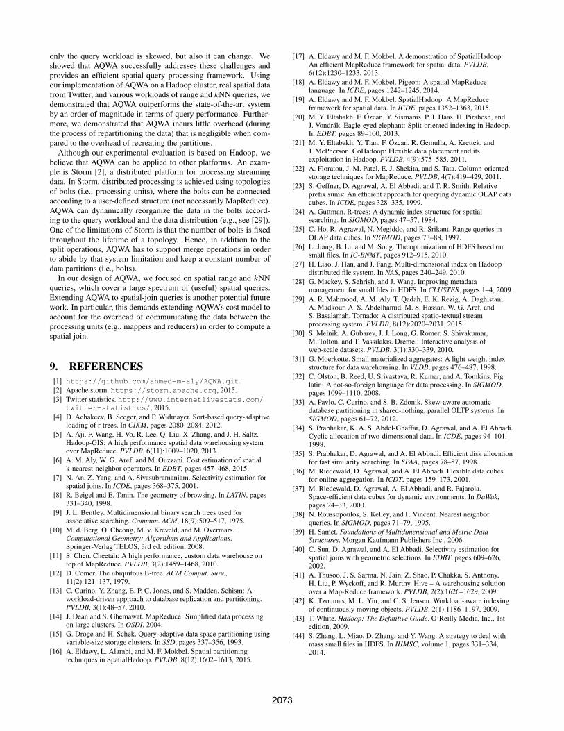
only the query workload is skewed, but also it can change. Weshowed that AQWA successfully addresses these challenges andprovides an efficient spatial-query processing framework. Usingour implementation of AQWA on a Hadoop cluster, real spatial datafrom Twitter, and various workloads of range and kNN queries, wedemonstrated that AQWA outperforms the state-of-the-art systemby an order of magnitude in terms of query performance. Further-more, we demonstrated that AQWA incurs little overhead (duringthe process of repartitioning the data) that is negligible when com-pared to the overhead of recreating the partitions.
Although our experimental evaluation is based on Hadoop, webelieve that AQWA can be applied to other platforms. An exam-ple is Storm [2], a distributed platform for processing streamingdata. In Storm, distributed processing is achieved using topologiesof bolts (i.e., processing units), where the bolts can be connectedaccording to a user-defined structure (not necessarily MapReduce).AQWA can dynamically reorganize the data in the bolts accord-ing to the query workload and the data distribution (e.g., see [29]).One of the limitations of Storm is that the number of bolts is fixedthroughout the lifetime of a topology. Hence, in addition to thesplit operations, AQWA has to support merge operations in orderto abide by that system limitation and keep a constant number ofdata partitions (i.e., bolts).
In our design of AQWA, we focused on spatial range and kNNqueries, which cover a large spectrum of (useful) spatial queries.Extending AQWA to spatial-join queries is another potential futurework. In particular, this demands extending AQWA’s cost model toaccount for the overhead of communicating the data between theprocessing units (e.g., mappers and reducers) in order to compute aspatial join.
9. REFERENCES[1] https://github.com/ahmed-m-aly/AQWA.git.[2] Apache storm. https://storm.apache.org, 2015.[3] Twitter statistics. http://www.internetlivestats.com/
twitter-statistics/, 2015.[4] D. Achakeev, B. Seeger, and P. Widmayer. Sort-based query-adaptive
loading of r-trees. In CIKM, pages 2080–2084, 2012.[5] A. Aji, F. Wang, H. Vo, R. Lee, Q. Liu, X. Zhang, and J. H. Saltz.
Hadoop-GIS: A high performance spatial data warehousing systemover MapReduce. PVLDB, 6(11):1009–1020, 2013.
[6] A. M. Aly, W. G. Aref, and M. Ouzzani. Cost estimation of spatialk-nearest-neighbor operators. In EDBT, pages 457–468, 2015.
[7] N. An, Z. Yang, and A. Sivasubramaniam. Selectivity estimation forspatial joins. In ICDE, pages 368–375, 2001.
[8] R. Beigel and E. Tanin. The geometry of browsing. In LATIN, pages331–340, 1998.
[9] J. L. Bentley. Multidimensional binary search trees used forassociative searching. Commun. ACM, 18(9):509–517, 1975.
[10] M. d. Berg, O. Cheong, M. v. Kreveld, and M. Overmars.Computational Geometry: Algorithms and Applications.Springer-Verlag TELOS, 3rd ed. edition, 2008.
[11] S. Chen. Cheetah: A high performance, custom data warehouse ontop of MapReduce. PVLDB, 3(2):1459–1468, 2010.
[12] D. Comer. The ubiquitous B-tree. ACM Comput. Surv.,11(2):121–137, 1979.
[13] C. Curino, Y. Zhang, E. P. C. Jones, and S. Madden. Schism: Aworkload-driven approach to database replication and partitioning.PVLDB, 3(1):48–57, 2010.
[14] J. Dean and S. Ghemawat. MapReduce: Simplified data processingon large clusters. In OSDI, 2004.
[15] G. Droge and H. Schek. Query-adaptive data space partitioning usingvariable-size storage clusters. In SSD, pages 337–356, 1993.
[16] A. Eldawy, L. Alarabi, and M. F. Mokbel. Spatial partitioningtechniques in SpatialHadoop. PVLDB, 8(12):1602–1613, 2015.
[17] A. Eldawy and M. F. Mokbel. A demonstration of SpatialHadoop:An efficient MapReduce framework for spatial data. PVLDB,6(12):1230–1233, 2013.
[18] A. Eldawy and M. F. Mokbel. Pigeon: A spatial MapReducelanguage. In ICDE, pages 1242–1245, 2014.
[19] A. Eldawy and M. F. Mokbel. SpatialHadoop: A MapReduceframework for spatial data. In ICDE, pages 1352–1363, 2015.
[20] M. Y. Eltabakh, F. Ozcan, Y. Sismanis, P. J. Haas, H. Pirahesh, andJ. Vondrak. Eagle-eyed elephant: Split-oriented indexing in Hadoop.In EDBT, pages 89–100, 2013.
[21] M. Y. Eltabakh, Y. Tian, F. Ozcan, R. Gemulla, A. Krettek, andJ. McPherson. CoHadoop: Flexible data placement and itsexploitation in Hadoop. PVLDB, 4(9):575–585, 2011.
[22] A. Floratou, J. M. Patel, E. J. Shekita, and S. Tata. Column-orientedstorage techniques for MapReduce. PVLDB, 4(7):419–429, 2011.
[23] S. Geffner, D. Agrawal, A. El Abbadi, and T. R. Smith. Relativeprefix sums: An efficient approach for querying dynamic OLAP datacubes. In ICDE, pages 328–335, 1999.
[24] A. Guttman. R-trees: A dynamic index structure for spatialsearching. In SIGMOD, pages 47–57, 1984.
[25] C. Ho, R. Agrawal, N. Megiddo, and R. Srikant. Range queries inOLAP data cubes. In SIGMOD, pages 73–88, 1997.
[26] L. Jiang, B. Li, and M. Song. The optimization of HDFS based onsmall files. In IC-BNMT, pages 912–915, 2010.
[27] H. Liao, J. Han, and J. Fang. Multi-dimensional index on Hadoopdistributed file system. In NAS, pages 240–249, 2010.
[28] G. Mackey, S. Sehrish, and J. Wang. Improving metadatamanagement for small files in HDFS. In CLUSTER, pages 1–4, 2009.
[29] A. R. Mahmood, A. M. Aly, T. Qadah, E. K. Rezig, A. Daghistani,A. Madkour, A. S. Abdelhamid, M. S. Hassan, W. G. Aref, andS. Basalamah. Tornado: A distributed spatio-textual streamprocessing system. PVLDB, 8(12):2020–2031, 2015.
[30] S. Melnik, A. Gubarev, J. J. Long, G. Romer, S. Shivakumar,M. Tolton, and T. Vassilakis. Dremel: Interactive analysis ofweb-scale datasets. PVLDB, 3(1):330–339, 2010.
[31] G. Moerkotte. Small materialized aggregates: A light weight indexstructure for data warehousing. In VLDB, pages 476–487, 1998.
[32] C. Olston, B. Reed, U. Srivastava, R. Kumar, and A. Tomkins. Piglatin: A not-so-foreign language for data processing. In SIGMOD,pages 1099–1110, 2008.
[33] A. Pavlo, C. Curino, and S. B. Zdonik. Skew-aware automaticdatabase partitioning in shared-nothing, parallel OLTP systems. InSIGMOD, pages 61–72, 2012.
[34] S. Prabhakar, K. A. S. Abdel-Ghaffar, D. Agrawal, and A. El Abbadi.Cyclic allocation of two-dimensional data. In ICDE, pages 94–101,1998.
[35] S. Prabhakar, D. Agrawal, and A. El Abbadi. Efficient disk allocationfor fast similarity searching. In SPAA, pages 78–87, 1998.
[36] M. Riedewald, D. Agrawal, and A. El Abbadi. Flexible data cubesfor online aggregation. In ICDT, pages 159–173, 2001.
[37] M. Riedewald, D. Agrawal, A. El Abbadi, and R. Pajarola.Space-efficient data cubes for dynamic environments. In DaWak,pages 24–33, 2000.
[38] N. Roussopoulos, S. Kelley, and F. Vincent. Nearest neighborqueries. In SIGMOD, pages 71–79, 1995.
[39] H. Samet. Foundations of Multidimensional and Metric DataStructures. Morgan Kaufmann Publishers Inc., 2006.
[40] C. Sun, D. Agrawal, and A. El Abbadi. Selectivity estimation forspatial joins with geometric selections. In EDBT, pages 609–626,2002.
[41] A. Thusoo, J. S. Sarma, N. Jain, Z. Shao, P. Chakka, S. Anthony,H. Liu, P. Wyckoff, and R. Murthy. Hive – A warehousing solutionover a Map-Reduce framework. PVLDB, 2(2):1626–1629, 2009.
[42] K. Tzoumas, M. L. Yiu, and C. S. Jensen. Workload-aware indexingof continuously moving objects. PVLDB, 2(1):1186–1197, 2009.
[43] T. White. Hadoop: The Definitive Guide. O’Reilly Media, Inc., 1stedition, 2009.
[44] S. Zhang, L. Miao, D. Zhang, and Y. Wang. A strategy to deal withmass small files in HDFS. In IHMSC, volume 1, pages 331–334,2014.
2073