..... AFGL-TR-84-O174

A STUDY OF TERRAIN REDUCTIONS, DENSITY ANOMALIES AND GEOPHYSICAL INVERSIONMETHODS IN GRAVITY FIELD MODELLING

,inhI~U~Rene Forsberg

The Ohio State University

00

.:) April. 1984

i "Scientific Report No. 5

-. "Approved for public release; distribution unlimited

AIR FORCE GEOPHYSICS LABORATORY

AIR FORCE SYSTEMS COMMAND4UNITED STATES AIR FORCE

HANSCOM AFB, MASSACHUSETTS 01731

VTCLECTE

041985

'C.,

v•gO•3, -

-"* ..":%i~* * '.

9:

CONTRACTOR REPORTS

This technical report has been reviewed and is approved for publication.

TqTOPW JE9L.1THOMAS P. ROONEYContract Manager Chief, Geodesy and Gravity Branch

FOR THE COQONDER

DONALD H.* ECKHARDTDirectorEarth Sciences Division

This report has been reviewed by the ESD Public Affairs Office (PA) and isreleasable to the National Technical Information Service (NTIS).

Qualified requestors may obtain additional copies from the Defense TechnicalInformation Center. All others should apply to the National TechnicalInformation Service.

If your address has changed, or if you wish to be removed from the mailinglist, or if the addressee is no longer employed by your organization, pleasenotify AIGL/DAA, Hanscom AFB, MA 01731. This will assist us in maintaininga current mailing list.

*7-°I

*16.

UnclassifiedSECURITY CLASSIFICATION OF THIS PAGE (when Date Entered)

REPORT DOCUMENTATION PAGE 1 READ INSTRUCTIONSI_ BEFORE COMPLETING FORM

I. REPORT NUMBER 12. GOVT ACCESSION NO. 3. RECIPIEN'r'S CATALOG NUMBER

AFGL-TR- 84-01744. TITLE (and Subtitle) S. TYPE OF REPORT & PERIOD COVERED

A STUDY OF TERRAIN REDUCTIONS, DENSITY ANOMALIES Scientific Report No. 5AND GEOPHYSICAL INVERSION METHODS IN GRAVITY FIELD

6MODELLING . PERFORMING 01G. REPORT NUMBER

OSU/DGSS-3557. AUTHOR(s) 0. CONTRACT OR GRANT NUMBER(s)

Rene Forsberg F19628-82-K-0022

9. PERFORMING ORGANIZATION NAME AND ADDRESS 10. PROGRAM ELEMENT. PROJECT, TASKAREA & WORK UNIT NUMBERSThe Ohio State University

Research Foundation 61102F1958 Neil Avenue, Columbus, Ohio 43210 2309G1BC

I I. CONTROLLING OFFICE NAME AND ADDRESS 12. REPORT DATEAir Force Geophysics Laboratory April 1984Hanscom AFB, Massachusetts 01730 13. NUMBER OF PAGES

Monitor/Christopher Jekeli/LWG 13314. MONITORING AGENCY NAME ADDRESS(if different from Controlling Office) IS. SECURITY CLASS. (of this report)

Unclassified

1Sa. DECLASSIFICATIONDOWNGRADINGSCHEDULE

16. DISTRIBUTION STATEMENT (of this Report)

Approved for public release; distribution unlirrited

17. DISTRIBUTION STATEMENT (of the ebstract entered In Block 20, It different from Report)

1. SUPPLEMENTARY NOTES

19. KEY WORDS (Continue on reverse side It necessary and Identify by block number)

Gravity field modelling, topographic/isostatic effects, empiricalcovariance functions, density anomalies

1 20. ABSTRACT (Continue on reverse side If necesary and Identify by block number)

,The general principles of the use of known density anomalies for gravityI ield modelling are reviewed with special emphasis on local applicationsand utilization of high degree and order spherical harmonic reference fields.The natural extension to include also unknown density anomalies will be studiedwithin the framework of geophysical inversion methods, and the prospectsfor or1hybrid"' -gravity field modelling/inversion methods will be outlined.A very simple case of such methods is the determination of representativetopographic densities through collocation with parameters.

DID I JAN7F 3 1473 EDITION Or I NOV 05S IS ODSOLETE Unclassified

* " /' / le SECURITY CLASSIFICATION OF THIS PAGE (*?oen Dot; Entoet-

. " . . .

-iii-

FOREWORD

This report was prepared by Rene Forsberg, Geodetic Institute, Denmark,and Research Associate, Department of Geodetic Science and Surveying, The OhioState University, under Air Force Contract No. F19628-82-K-0022, The Ohio StateUniversity Project No. 714274. The contract covering this research is administeredby the Air Force Geophysics Laboratory, Hanscom Air Force Base, Massachusetts,with Dr. Christopher Jekeli, Scientific Program Officer.

Certain computer funds used in this study were supplied by the Instructionand Research Computer Center through the Department of Geodetic Science and Surveying.

This report is a contribution to a gravity field modelling project supportedby NATO grant no. 320/82. Travel support for the author's stay at The Ohio StateUniversity have been provided by a NATO Science Fellowship grant.

The author wishes to thank Dr. Richard H. Rapp for hosting me at OSU andvaluable disucssions, Laura Brumfield for typing the report and finally a specialthanks to the many graduate students of the Department who have helped me, throughfruitful discussions and through practical advice, especially how to tackle thecomputer system at OSU. An additional thanks to Jaime Cruz for putting to mydisposal some of his p'ots.

Ace3sion For,,TT%- GRA&IDTTC TABU-'announcedJJit i c t i on--

L17 rl rbut ioil/

A-:: -.'."L ity Codes :-il nni/or"

I

Ir..w-" . ' - ' .'.,J-,'-, •-- . . - . . - • "* -- ." .. ..-" .- , ,' ...*. ** * .-.' , .-.',',." . . .. ..

-iv-

CONTENTS

1. Introduction 1

2. The Anomalous Gravity Field and Density Anomalies 6

1. On the Use of Spherical Harmonic Expansions 9

4. Utilization of Known Density Anomalies 14

5. Unknown Densities - Geophysical Inversion 16

6. Density Modelling Using Rectangular Prisms 246.1 Space Domain 246.2 Frequency Domain 28

7. Terrain Reductions 337.1 Terrain Effects and Associated Density. Anomalies 347.2 Practical Terrain Reductions in Gravity Field Modelling 407.3 The Linear Approximation for topographic Effects 427.4 Accuracy of the Linear Approximation 467.5 The Terrain Correction as Convolution Integrals 507.6 The Use of FFT for Terrain Effect Computations 527.7 The Linear Approximation and Error Studies 577.8 Error Studies of DTM Resolution Requirements 60

8. Spectral Characteristics and Covariance Functions for Local Topographyand Terrain Effects 688.1 Topographic Covariance Functions for U.S. Sample Areas 738.2 Magnitude of the Gravimetric Terrain Correction - Colorado Area 788.3 RTM Geoid Effects - Colorado Area 82

9. Terrain Reductions: Spectral Characteristics and Covariance FunctionsFor Local Gravity in U.S. Sample Areas 85

10. Isostatic Reductions of Satellite Altimetry Data in Two Areas of thePacific 94

11. Summary and Conclusions 107

Appendix: TC - A FORTRAN Program for General Terrain Effect 111Computations

References 127

X:

II

- . . . . . . . .. .. . .... ..... U11 .. . . U . . .*' . . .

41 -1-

1. Introduction

With the term "gravity field modelling" we usually, in the geodetic community

mean methods for representing the external potential of the earth, in order to

be able to estimate quantities related to the gravity field from a given set of

"observed" quantities. Such methods include spherical harmonic expansions, integral

formulas such as Stoke;' and Vening-Meinesz' formulas and "spatial" approximation

methods such as c6llocition and generalized point mass modelling (e.g. Bjerhammar's

methods). Common for ill of these methods is that they are approximation methods

for harmonic functions, all rely on the assumption that the anomalous potential

T fulfills Laplace's *?quation v 2T = 0 at least outside the surface of the earth.

No assumption is made regarding the density distribution actually generating the

gravity field.

In contrast the term "gravity field modelling" as used in geophysics stands

for the process of determining internal density distributions of the earth, consis-

tent with the observed outer field. This inversion is non-unique, and to get

reasonable answers the geophysicist must introduce constraints, through selection

of a finite dimensional representation of the structures (density values, depth

parameters, etc.), through "fixing" some of these parameters based on independent

geophysical information (well data, seismic interpretations) and through subjective

choices of the most "realistic" models in terms of geology. At the basis of the

geophysical gravity field modelling is the "direct problem" of potential field

theory: to calculate the gravity potential and its derivatives in space due to

6 • given density distributions.

When the prime interest is in "external" gravity field modelling, any geophysical

density model, realistic or not, may in principle be used to represent a part

of the external field through a direct computation of the effects of the assumed

-2-

density distribution. If the density distribution is realistic we would expect

the remaining field to be more smooth, in some cases the fit would be so close

that we would have no use for any external gravity field modelling at all. Usually,

however, our knowledge of density anomalies is confined to more shallow structures

of crustal and upper mantle origin, thus mainly contributing to the shorter wavelengthe$

of the variation of the gravity field. Longer wavelength parts of the signal are

more conveniently treated using "external" modelling, such as high degree and

order spherical harmonic expansions of the geopotential.

The "external" and "internal" modelling may conveniently be done simultaneously

in some cases, using e.g. combined versions of collocation and geophysical inversion

procedures. Thus we will at the same time estimate both the external gravity

field and density values inside the earth. This approach has the advantage that

it allows fairly easy use of independent geologic/geophysical information as data

for the construction of external gravity field models. Due to the difficult choice

of geologically "reasonable" density parameters it will, however, hardly ever

be a "hands-off" automatic method like standard collocation.

Combined collocation/inversion will probably prove itself useful for inversion

of future "multisensor" gravity data, as e.g. gravity vector measurements by

inertial survey systems and gravity gradiometer measurements. In conventional

geophysical inversion we have an inherent arbitrary choice of the "regional" field,

representing the effects of all other sources than the density structures of interest.

This regional/residual - separation is done using more or less crude forms of

filtering and trend fitting. When we have several different types of gravity

field data containing information about the same mass body, it is essential that

the filtering is consistent between the various gravity field data types, such

that the filter output still represent quantities related to the same harmonic

function. This will be assured using combined collocation/inversion and similar

methods.

"6 :-:'. ,- :'1 " ,' , -.,-- , -. " . " .-. '- . , :': -.: ," ' - :,. ..- . , :.. ''1 - . . - , ., .

-3-

In this report tie utilization of density anomalies for genereralized gravity

field modelling will be treated in the first chapters in a rather broad way.

The bulk of the report will, however, be concerned about the most important and

also best known density anomalies on the earth, namely density anomalies associated

with the topography.

The density anomalies relating to the topography include the direct gravita-

tional effects of the visual topography on the continents, the ocean bathymetry,

ice cap effects and the isostatic compensation. These effects together represent

a major part of the variation of the earth's gravity field, especially at shorter

wavelengths (less than, say, a few hundred kilometers), where the direct computed

topographic effects only to a low degree are counteracted by the isostatic compensa-

tion effects. In mountainous areas the topographic effects completely dominate

the local variation of the gravity field, and some kind of terrain reduction is

indispensable when attempting gravity field modelling in such areas. The most

well-known terrain reduction is the Bouguer reduction, which is well-suited for

geophysical work and prediction of mean free-air anomalies (for use e.g. in tradi-

tional geodetic gravity field modelling), but is not applicable for reduction

of geoid undulations. Isostatic reductions provide the smoothest possible residual

fields on a global basis, and are easily applicable to all the various types of

gravity field data available. The computation of topographic/isostatic effects

is facilitated by high-degree spherical harmonic expansions of the isostatic reduc-

tion potential (Rapp, 1982), but for local applications the computations are still

relatively laborious. Since the usual Airy-type isostasy does not operate on

a local scale (the short wavelength topography is supported by the finite strength

*'. of the earth's crust) we might not like to introduce the somewhat arbitrary isosta-

tic reduction mass anomalies at the crust/mantle boundary. Instead we might just

I simply try to take only the short wavelength variations of the topography into.!

........................................... ~ .. ... ... ... ...

-4-

account,introducing an arbitrary smooth mean elevation surface ("model" earth)

as a "reference" topography, the gravitational influence of which is not directly

taken into account in the gravity field modelling. For gravity anomalies such

a residual terrain correction corresponds closely to the formation of regional

mean free-air anomalies, and by choice of a proper reference elevation surface,

such as defined through a spherical harmonic expansion of the earth's topography

to degree and order 180, we end up with a reduction which would be expected to

give somewhat similar results as conventional isostatic reductions.

For local modelling of the gravity field - on which the main emphasis is

put in this report - the availability of high degree and order spherical harmonic

expansions of the geopotential (Lerch et al., 1981; Rapp, 1982) has proven itself

to be a major break-through of big practical value. For a region like Scandinavia

with reliable l0x 10 mean gravity data, the r.m.s. variation of the gravity anom-

alies is roughly reduced to half the original value, and geoid undulations may

be computed with an accuracy around 1 m using such spherical harmonic expansions

(Tscherning, 1983). Thus by using long-wavelength information from such expansions

and combining with short and medium wavelength topographic effects computed using

a residual terrain model with respect to a corresponding spherical harmonic expan-

sion of the topography itself, the "remaining" signal will be smooth, its variance

low and its degree of anisotropy usually less. This will be demonstrated later

in this report, through investigations of local empirical covariance functions

and power spectra of the gravity field in areas with different types of topography.

The computation of terrain effects, using digital terrain models, is basically 4

a problem of numerical integration. However, it is by no means a simple problem.

The integration kernels are usually singular at the evaluation points, and the

influence of the "inner zone" - the topogriphy in the immediate vicinity of the

evaluation point- is very critical for quantities like gravity anomalies and second

r- LIL I

-5-

order derivatives. A FORTRAN program for computing terrain effects on geoid undulations..

deflections of the vertical and gravity anomalies, based on the rectangular prism

as integration element, will be given in the appendix.

For gravity anomalies a type of topographic effect - the conventional gravi-

metric terrain correction - is of special interest. The terrain correction is

basically not a terrain reduction, used in conjunction with a general gravity

field modelling procedure it represents no unique density anomaly distribution

to be removed from the observations. Rather the terrain correction should be

viewed as a mathematical convenience, representing the - usually small - nonlinear

part -I the total terrain effect. Unfortunately terrain corrections have from

time to time been confused with terrain reductions proper. The application of

terrain corrections alone does usually not improve results of the gravity field

modelling in mountainous areas significantly, since the bulk of the topographic

density anomaly distribution, causing short wavelength "noise" in the gravity

field, is not removed. The application of terrain corrected free-air anomalies

.* does, however, make good sense for integral formula applications, since the applica-

tion of the terrain correction to free-air anomalies represents a first (and rather

crude) approx-imation to the problem of downward continuation of gravity observations

from the surface of the topography to the geoid, the terrain correction being

an approximation to Molodensky's G 1-term, see e.g. Heiskanen and Moritz (1967)

4 and Moritz (1966). The role of the terrain correction will be given attention

later in this report, and some examples of its magnitude will be given.

To summarize, the emphasis in this report will be on the utilization of density

anomalies in local gravity field modelling - especially collocation and related

methods. The first part will review principles for the utilization of known and

unknown density anomalies, then the practical computation of such effects -

especially topographic effects - will be outlined, and finally the influence of

~~~~~~~~~~~~.'_.'...'.. .......-......-.........,............... .....° ............. ..... .....-.-. . . . . ._

-6-

the topography will be stuaied through investigations of empirical covariance functions

for various test areas in the United States. No major examples of actual applications

of the methods for gravity field modelling will presently be given. For earlier

results of gravity field modeling by collocation using some of the terrain reduction

concepts presented, the reader is referred to e.g. Forsberg and Tscherning (1981),

Forsberg and Madsen (1981), and Tscherning and Forsberg (1983).

2. The Anomalous Gravity Field and Density Anomalies

The gravity field of the earth is traditionally described using the anomalous

potential T

T = W- U (2.1)

representing the difference between the actual geopotential W and a normal poten-

tial U, corresponding to chosen reference ellipsoid parameters. In U is also

included the centrifugal, tidal and atmospheric potentials, and thus T is a

harmonic function.

72T 0 (2.2)

outside the surface of the earth, and may be expanded in spherical harmonics

GM RT(r, r a ( ) 7 (Yu) (2.3)

t 2 m- zn r

) Pzm (sin €) cos mx (m > 0)

Un P = (sin ¢) sin mx (m < 0)Im

Here G is the gravitational constant, M the mass of the earth and R the radius

of a reference earth sphere (Bjerhammar sphere).

I

o.-" . .. .. . . - - . .. • . - .' - . - -. ' . . .. . . ." ' .. . *. - ." .* ". - - " ." . '' .

-7-

The observable gravity field quantities may in the usual spherical approx-

imation be expressed as linear functionals L(T), the most important quantities

being point and area mean values of

Height anomalies/geoid undulations (2.4)'Y

_ ~ _ 3T -,

ry a IDeflections of the vertical (2.5)

r-y cos 3

L IT- T Free-air anomaly (2.6)-r r

T6g= -r Gravity disturbance (2.7)

where y is normal gravity.

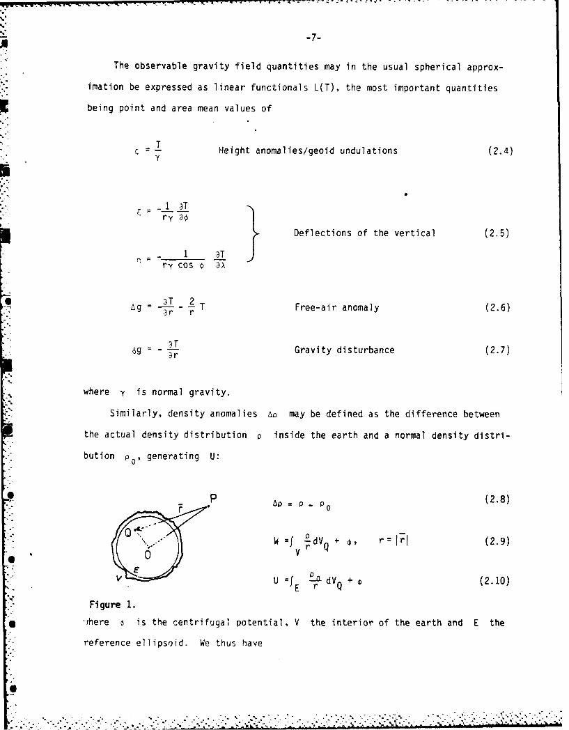
Similarly, density anomalies Ao may be defined as the difference between

the actual density distribution p inside the earth and a normal density distri-

bution P0 ' generating U:.0

P p P (2.8)

W =f -adVQ + , r r (2.9)r

V

E r dV +0 (2.10)

Figure 1.*..ihere b is the centrifugal potential, V the interior of the earth and E the

reference ellipsoid. We thus have

.. . . .- -- .. .k . .-

JOW -8-

T(P) = PV r dV (2.11)

In other words, Ap is a density distribution generating the anomalous gravity

field.

Due to the fundamental ambiguity of potential field theory, an infinite variety

of density distributions satisfying (2.10) exists. If a spherical normal potential

U is chosen, indeed any radial symmetric density distribution, having the correct

GM-value, generates U. It is therefore clear that- the observed gravity field

• is of no use in determining a realistic normal density p 0. Instead we must get

information on p0 from other geophysical sources: seismic body-wave travel

times, surface wave dispersion curves, eigen periods of the earth's free oscilla-

tions and the moment of inertia. Examples of current earth models, applicable

for "defining" Po' is the HB-I (Haddon & Bullen, 1969) model and the PEM-models

(Dziewonski et al., 1976).

To account for the non-spherical part of p0 we may resort to perturbing

the interior density distribution by small amounts, given by the hydrostatic equili-

brium theory. The flattening of the interior density discontinuities will thus be

decreasing downwards, from 1/298 at the surface to 1/390 at the core/mantle bound-

ary. Alternatively we may resort to a stringent analytic representation of the

normal density distributions using ellipsoidal coordinates (where the flattening

increase with depth), and more orlessarbitrary mathematical constraints to secure

a unique solution (Moritz, 1968; Tscherning&Sunkel, 1980). In any way, however,

the non-spherical perturbations are very small, much less than the errors in the

geophysical earth models, and we may thus for all practical purposes simply disre-

gard these.

0 - ° - • " ° " . ' . ° - " °, " ' ' ' " "•" ° ° " *° . • " • . i

-9-

We are thus free to choose "convenient" reference density distributions when

working in given regions: a typical continental choice would be e.g. a density

starting at 2.67 g/cm 3 at sea level, increasing to 2.9 at the base of the crust,

jumping to 3.3 across the moho at 32 km depth and increasing through the mantle

with major "discontinuities" at the phase transition zones at -420 km (olivine-spinel)

and at -700 km. At tte base of the mantle the PEM-model gives a density of 5.4,

and for the earth's c(re values from 9.9 to 13.0 at the center, the density of

the inner core being still very uncertain. For an oceanic area we might change

this model above the low velocity zone, e.g. choosing a reference model with 4 km

of water (density 1.02), a thin, dense crust (2.9) extending to 12-18 km depth

and an "undepleted", cceanic upper mantle at 3.4g/cm3.

3. On the Use of Spherical Harmonic Expansions

When we use a spherical harmonic expansion as a first step in gravity field

modelling, the "wanted" approximation T to T is split into

+ (3.1)

with i given by the expansion

4ma x

T r~,)L~~ a (!Y (0, A) (3.2)r Z=2 m=- m r Ym

The currently available high degree-and-order models (tmx = 180) provides the

bulk of T. rfey suffer, however, of a minor problem relating to the continental

topography: information on the higher-degree coefficients stem from analysis

of lox 10 E-g (used directly in the Rapp models (Rapp, 1981) and through Stokes'

formula in GEMIOC (Lerch et al., 1981)), treated as data on a sphere, neglecting

that the continental anomalies are actually anomalies at altitude. This fact

gives rise to a small correction, completely corresponding to Molodensky's

G-term, but in the frequency domain.

i%

- 10-

Let the standard surface harmonic expansion of the mean anomalies be

~GM

Ag(O, A) GM R U-1) a m Y m(O' X) (3.3)m

To first order these anomalies correspond to elevation h(, A), defined through

a similar expansion of the continental topography (0 at oceans). Using the correct

spatial expansion (3.2) we get

GM R (34)Ag -R 2T (t-1) aI m (- ) Y (.4

(R+h) X m R+h

SGM (3.5)

(i2 U (-1) a m(1- X) M(35

Xm

.- GM -F (Y-i)(t+2) am Y (3.6)

where Eg* is the gravity anomalies harmonically downward continued to the

Bjerhammar sphere. Since a aI m', the second term in (3.6) may be evaluated

with sufficient accuracy from existing solutions, representing essentially

h • T z Expanding this correction term in surface spherical harmonics b weZ m1

obtain

A- = . - GM b (3.7)

which by (3.3) and expansion of Ag* gives

a =m a'm +Z bm (3.8)

The correction term has for gravity anomalies a maximum value of c. 19 mgal (Rapp,

1983). For local gravity field modelling the above has the practical application

that elevations of the individual (ground) observation points should be used

4, properly when evaluating (2.3), otherwise elevations should rather be set to zero.

,"

-11-

Corresponding to (3.1) also the density anomaly may be split in a spherical

harmonic reference part and a residual

AP P + 6 (3.9)1 2

The reference density distribution Ao1 poses some problems, especially for high

degree-and-order fields (imax ? 180), since many of the major crustal -upper-

mantle structures (trenches, rifts, etc.) will indeed have a significant part

of their gravitational signal in the reference part Ap When working with

residuals ("T ") only. the response from assumed Ao-models must thus be split,2

either by introducing a "formal" Ap1 , or by high-pass filtering the response.

In this case we will, however, lose important information about the structure.

For more local gravity field modelling, we may totally neglect the density

split (3.9). Many of the typical intracrustal density anomalies would have only

small long-wavelength effects. By removing such density anomalies computationally,

the remaining part of the residual potential T would in principle be "con-2

taminated" with these long wavelength errors, but they will usually not be very

significant compared to e.g. the errors in the reference field T

For the topography, the natural choice of Ap would be a model corresponding

to an analogous expansion in spherical harmonics of the topographic elevations:

9-max th m (,) (3.10)

1 m=-q m I

The reference density model in this case would have density-2.67 g/cm 3 below

the mean elevation surface h(o, x) on the continents. More on this (i.e., the

residual terrain correction) later.

Formal introduction of spherical harmonic reference density anomalies

may be done using simple analytical inversion methods. Consider e.g. a two-layer

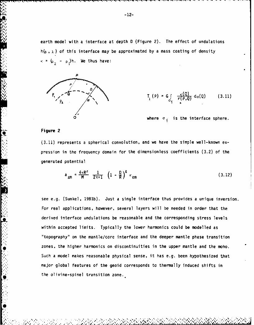
-12-

earth model with a interface at depth D (Figure 2). The effect of undulations

h(o, ) of this interface may be approximated by a mass coating of density

2 - p )h. We thus have:

T (P) = Gf r da(Q) (3.11)

pS

19 Gi

• \P- 70i

0 where a i is the interface sphere.

Figure 2

(3.11) represents a spherical convolution, and we have the simple well-known ex-

pression in the frequency domain for the dimensionless coefficients (3.2) of the

generated potential

am M 2 (+I I -R/ K Xm (3.12)

see e.g. (Sunkel, 1981b). Just a single interface thus provides a unique inversion.

For real applications, however, several layers will be needed in order that the

derived interface undulations be reasonable and the corresponding stress levels

within accepted limits. Typically the lower harmonics could be modelled as

"topography" on the mantle/core interface and the deeper mantle phase transition

zones, the higher harmonics on discontinuities in the upper mantle and the moho.

Such a model makes reasonable physical sense, it has e.g. been hypothesized that

major global features of the geoid corresponds to thermally induced shifts in

the olivine-spinel transition zone.

• " ~~~~~~~~~~~~~~~."........... .. ............ . .......... -.... .. ''.-.'...'.'-',','.--',. .. ,''........

-13-

Alternatively, unique "spatial" density anomaly models may be obtained by

imposing "analytic" constraints on the possible density distributions. If e.g.

the density distribution fulfills the condition

v2(rnc) = 0 (3.13)

where n is a'n arbitrary integer constant, the density solution is found by an

expansion in internal spherical harmonics as

o(r, n, ) rny b ) Y'm (b' A) (3.14)Im

with

bit= (2z - n + 3)(2z + 1) (3.15)",b m 47TGR3-h aXm•

for 2z > n - 3 (Tscherning, 1974). The drawback of this method is that the con-

dition (3.13) is completely arbitrary without any physical meaning. The resultant

density distribution will have its extremes atthe surface of the sphere, and the

actual density variations will be very low - e.g. order-of-magnitude 0.004 g/cm3

for GEMIOB (Imax = 36) (Tscherning & Sunkel, 1980). Attempts to find other constraints

like (3.13) corresponding to some simple physical minimum principle have been

fruitless (Tscherning, personal communication) - it is obviously not possible

to find "state equations" for the earth's interior relating only to the density

distribution.

tI

°I

%'I

-14-

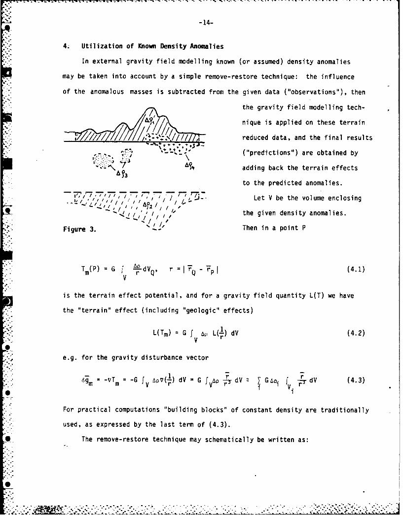
4. Utilization of Known Density Anomalies

In external gravity field modelling known (or assumed) density anomalies

may be taken into account by a simple remove-restore technique: the influence

of the anomalous masses is subtracted from the given data ("observations"), then

the gravity field modelling tech-

nique is applied on these terrain

reduced data, and the final results

-- t.- ("predictions") are obtained by

.-.- ,\7 at adding back the terrain effects

to the predicted anomalies.

./ ,' /;, ,,,'/-... Let V be the volume enclosing

/ / the given density anomalies.

Figure 3. /' Then in a point P

TmP) G ALr VQ r =IT_ " -pl (4.1)

V

is the terrain effect potential, and for a gravity field quantity L(T) we have

the "terrain" effect (including "geologic" effects)

L(Tm) = G fV Ap L(!) dV (4.2)V r

e.g. for the gravity disturbance vector

= -vT m = -G f AO7(1) dV = G r,,p __ dV I G ,oi v T 4dV (4.3)r 1

For practical computations "building blocks" of constant density are traditionally

used, as expressed by the last term of (4.3).

The remove-restore technique may schematically be written as:

. . . . . . . . . . . .. . . U. .. - .-:. .. ', . ,..:. *.. - . ;U.. :" . . .. .- ..-.

-15-

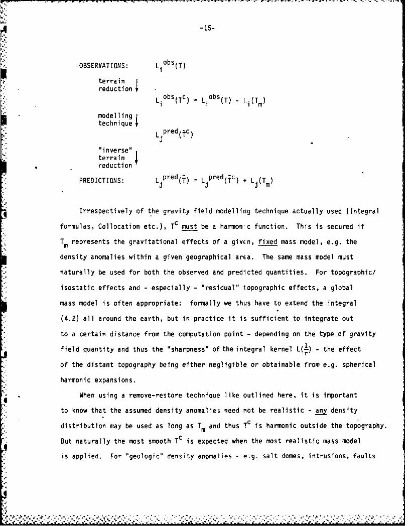
OBSERVATIONS: Lio(T)

terrainreduction

LiobS(Tc) L bS(T) - L.(T)

modellingtechnique

Ljpred(-c)

"inverse"terrainreduction

PREDICTIONS: Ljpred(T) L pred(Tc) + L.(T M)

Irrespectively of the gravity field modelling technique actually used (Integral

formulas, Collocation etc.), Tc must be a harmon-c function. This is secured if

Tm represents the gravitational effects of a givEn, fixed mass model, e.g. the

density anomalies within a given geographical arEa. The same mass model must

naturally be used for both the observed and predicted quantities. For topographic/

isostatic effects and - especially - "residual" topographic effects, a global

mass model is often appropriate: formally we thus have to extend the integral

(4.2) all around the earth, but in practice it is sufficient to integrate out

* to a certain distance from the computation point - depending on the type of gravity

field quantity and thus the "sharpness" of the integral kernel L(-!) - the effectir

of the distant topography being either negligible or obtainable from e.g. spherical

harmonic expansions.

When using a remove-restore technique like outlined here, it is important

to know that the assumed density anomalie3 need not be realistic - any density

distribution may be used as long as Tm and thus Tc is harmonic outside the topography.

But naturally the most smooth Tc is expected when the most realistic mass model

is applied. For "geologic" density anomalies - e.g. salt domes, intrusions, faults

- , - ..- .....- ,.. . ... -.. -. - *....... ...... ... . .. .. ,... . .. ..* . .... .B-.. .-. .

-16-

etc. - even the simplest models (spheres, cylinders, step functions) may often

be applied successfully, to give a more stationary and isotropic residual field,

well-suited for interpolation and approximation.

5. Unknown Densities - Geophysical Inversion

Most frequently we do not have a good knowledge of "geologic" density

anomalies, and it would therefore be natural to try to estimate parameters des-

cribing such density anomalies - preferably simultaneously with the external

gravity field modelling process. In addition to the obvious importance of know-

ledge of the surface density distribution, we will by this method also have a

0 simple way of introducing non-gravity observation data (magnetic, seismic etc.)

in the external gravity field modelling. Simple but very essential geodetic

applications includes determination of optimum topographic reduction densities

(generalized Nettleton method) and e.g. determination of ocean bathymetry in un-

surveyed areas from satellite altimetry.

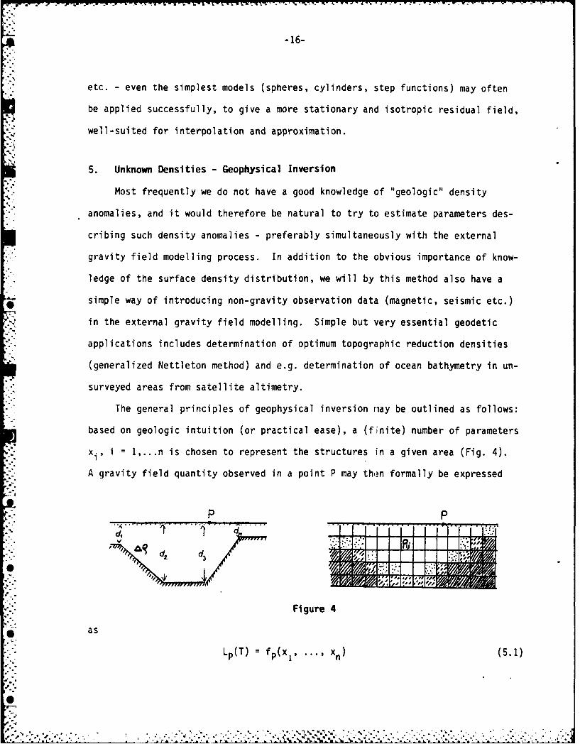
The general principles of geophysical inversion nay be outlined as follows:

based on geologic intuition (or practical ease), a (finite) number of parameters

xi , i = 1,...n is chosen to represent the structures in a given area (Fig. 4).

A gravity field quantity observed in a point P may then formally be expressed

P P

d3

Figure 4

as

Lp(T) = fp(x1, ... , xn) (5.1)

0n

,7

-17-

where the function fp is generally non-linear and must be linearized

(Lp(T) - LO(T))= i (5.2)

i axi 0

by assuming an initial model x?. Since geophysical inversion problems are oftenI"

highly nonlinear, a large number of iterations (5.2) are often necessary. The

model parameters x. may be generally classified in two types:

1) geometric parameters (interface depths etc.)

2) density value parameters

The main emphasis in traditional geophysical modelling has been in terms

of structural geometric parameters (see e.g. Burkhard & Jackson, 1976; Pedersen,

1979), to directly represent interfaces such as the top basement in sedimentary

basins or the moho, exemplified in Figure 4 (left). The advantage of the geo-

metric parameters is that they directly reflect simplified geologic models, and

additional data such as well control is easily including by e.g. fixing one or

more parameters. The drawback of choosing "structural" parameters is the inherent

unlinearities.

Opposed to this, models with density value parameters only (Figure 4, right)

are perfectly linear, but the computational advantage of the linearity is usually

counterweighted by the greater number of parameters needed to represent a wanted

geologic scenario. Also it is less simple to include the non-gravity constraints.

The commonly applied point mass modelling in geodesy may be viewed as a special

case of such geophysical inversion, using the simplest possible finite element

representation (delta spikes) of the subsurface density distribution. However,

this simplest possible case of inversion gives results that are amazingly close

to results obtained using improved (spatial) density representations (Figure 5).

I

N 4- 1 -so 0 C-

M~- E i

-0 co = a

'~4-. 4-V

0 h,

La.. nl F n LA.j

(AA

I-.-

* ~* CV

xaJ E (A,

C -

- -.-... .. - - * - T

-19-

Assuming a set of observations yi = Li(T), i = 1,...,n the (linearized)

inversion geophysical problem may be written as

y = A< (5.3)

where A is the response matrix. This problem is generally ill-conditioned or

improperly posed, and generalized invers on must not be used.

One popular technique is the use of the singular value decomposition:

A = UAVT, A (5.4)0 "p

with the U and V being orthonormal matrices defined through

ATAv. = Aqv. V = {v.}

(5.5)

AATu : X2u U = {uj}

See e.g. Pedersen (1979) or Rummel et al. (1979). p is the number of non-zero

eigen values, i.e. the number of degrees of freedom of the problem. A solution

x to (5.3) is given by the Lanczos inverse,

= VA 'Uy (5.6)

*T Tminimizing as well y y as x x. To prevent the eigen values of ill-conditioned

problems to induce large changes in the parameters x, the eigen value spectrum

A may be truncated by removing eigen values smaller than a suitable threshold,

giving the traditional trade-off between resolution and variance.

Alternatively to the explicit use of the singular value decomposition, es-

sentially the same solution may be obtained using Tikhonov regularization. In

this case we seek to minimize a combination.

,

-20-

Ily " Ax 112 Ix 112, > 0 (5.7)

Assuming a noise covariance matrix D for the observations and an a priori covariance

matrix C for the "signal" x (both matrices usually assumed to be diagonal), we

obtain the solution by solving the normal equations.

A (AT D IA + aC')x = ATD y (5.8)

(Rur.mel et al., 1979). The constant a is arbitrary and may be chosen to obtain

a desired smoothness of the parameters, again with the price to be paid being

a degraded fit of the model.

Independent geologic information may be taken into account using linear con-

*0 straints of the form

Bx C (5.9)

where B and C are constant. Such constraints can be used to fix certain

parameters (e.g. representing known depths to an interface), to fix differences

in density values (e.g. forcing parameters of type "2" to represent layers, faults,

etc.) and to introduce special geometric constraints on the anomalous mass body

based on geologic experience (e.g. issuming a dike to have parallel sides).

The constraint (5.9) is taken into account in the minimization problem (5.8) using

Lagrange multipliers, obtaining somewhat more complicated normal equations.

Details may be found e.g. in Burkhard & Jackson (1976).

The methods outlined above represent conventional geophysical inversion tech-

0 niques. They are usually applied only for one type of gravity field quantity

(gravity anomalies or - at times - altimeter geoid undulations), but there is

of course no restriction in the model formulation to utilize heterogeneous data

(e.g. simultaneous gravity and geoid information) as we are commonly used to in

geodesy. The problem with the hetetogeneous data lies in the regional/residual

separation: .the gravity field contiins inf)rmation about density anomalies at

. . . ....0..

-21-

all depths, but the model parameters x are typically restricted to describe

simplified rather shallow structures - a filtering is therefore done to remove

the unwanted parts of the signal. This filtering is often very crude (e.g. graph-

ical determination of a "regional") and not applicable for heterogeneous data,

for such data we must make sure that the filtering of the different data types

are consistent - the "regional" must be a harmonic function.

In some cases high degree and order sphErical harmonic expansions might be

valuable as "regionals" - e.g. when trying tc model total crustal density distri-

butions-but we should then also have a well-aefined spherical harmonic reference

density distribution (c.f. Section 3). Alternatively we can utilize "general"

gravity field modelling techniques to represent the regional, e.g. by introducing

arbitrary (deep) model point-masses or by doing the inversion within the framework

of least squares collocation with parameters.

In this case we have the following observation equations for an observation

yi with associated linear functional Li ard noise ni:

Yi = Ax}i + Li(T) + ni (5.10)

for which we get the well-known collocation solution (see e.g. Moritz, 1980)

T(Q) = L iK(.,Q) T C-1

= A)- ATCIy (5.11)

C = {LiL.K(-,.) + Dij.

where D again is the noise covariance matrix, K(P, Q) the potential covariance

function of the gravity field. Note that this covariance function should not

be the observed, empirical covariance function but rather the covariance function

of the field after the model influence have been subtracted - i.e. the covariance

function of the "regional". We would expect this field to have less variance

and greater correlation length than the original field. Since the model results

I

. . . . . .

*-22-

depend on the covariance parameters, these must ultimately be determined through

trials or through considerations of the wanted characteristics of the regional/

residual filter.

Least squares collocation with parameters will be especially well-suited

for the determination of optimum topographic reduction densities in mountainous

areas. In this case our model parameters x will just be a single value (or

a few, if the geology is changing), and the observation equation (5.10) will look

like

Yi (G f Li(1)dV1Ap + Li(T) + ni (5.12)S V1 r(.

where the term in the bracket repre:sents the terrain effect of a topography with

unit density, cf. (4.2). This prob em is well-conditioned for sufficiently

varying topography, and represents .a straight forward generalization of

Nettletons density profilinc method to heterogeneous data. More reliable density

estimates are obtained with (5.12) ;han with the more traditional approaches such

as regression analysis of t~e varia:ion of free-air anomalies with elevation,

as pointed out by Sunkel (181a). Application of (5.12) will probably be even

better than using real meastrements of sample rock densities: everybody who has

tried this knows how difficilt it i'; to estimate average formation densities from

samples of individual rock formations, especially for sedimentary rocks with their

varying porosity and water saturation.

When estimating more complex structural models of the density anomalies,

stabilization of the parameters i in (5.11) will be needed, and we will have

to make a combined collocation/.Ieneralized inverse approach. Collocation by itself

may be viewed as an inversion problem (Moritz, 1976): the simple collocation

approximation T is built up from the kernel function K(P, Q) in the observation

4- points:

I0j.........O

-23-

T(Q) L aL.K(,Q) (5.13)

where the coefficient a. is the solution fo the "normal equations" corresponding

to (5.11). Expressing (5.6) in terms of these coefficients we have:

y= Ax + L.L.K (,.) a. + n.3 3 I

(5.14)

(A {L .L.K(- ,-) ({ + n ~i

which clearly shows our problem as a "double" generalized inverse problem with

unknowns xj. (geophysical parameters) and a. (kernel coefficients). The solution

is obtained by minimizing a combination:

lx l2 + a- Tl1 (5.15)

where a is a positive constant and 11 IIH the Hilbert space norm associated with

the chosen covariance function K. The constant a is arbitrary, and must be

chosen based on empirical investigations. The constant determines how much vari-

ation is put "into" the structure and how much is retained in the outer, residual

field, and acts like the "trade-off" parameter in (5.7). By combining the well-known

methods of collocation and geophysical generalized inversion like outlined here,

we have in fact obtained a discrete version of the so-called "mixed collocation",

suggested by Sanso and Tscherning (1982).

The practical applicability of hybrid gravity field modelling/geophysical

inversion methods remains to be seen. For geodesy and external gravity field

4 modelling the obvious application would lie in the determination of only a few

key parameters: topographic densities, density contrasts across major known discon-

tinuities (e.g. for moho at continental margins) and densi:y anomalies of well-known

* geologic bodies (e.g. salt domes), avoiding unlinear struclural parameters requiring

iteration. The computational burden would not be significantly increased using

"k

-24-

such a limited set of parameters, and by choosing "good" geologically reasonable

parameters, one could hope in many cases to get significant improvements in the

characteristics of the "background" field: less power, more stationarity and

a higher degree of isotropy.

Probably the geophysical exploration would benefit more from the hybrid col-

location/inversion scheme. With the technological advances heterogeneous gravity

field data will be more common - through the development of high-precision inertial

survey systems measuring the complete gravity vector, through airborne gradiometry

and through geoid undulations irom GPS and satellite altimetry in addition to

terrestrial or airborne gravity. To perform quantitative interpretations with

error analysis etc. for such data, some kind of "hybrid" inversion method will

be necessary, to stringently handle model oversimplifications, regional/residual

separations etc.

With these remarks the general discussion of density anomalies and inversion

techniques will be concluded. In the next section formulas for actual computations

will be given,and then the main den;ity anomaly - the topography - will be treated

in detail.

6. Density Modelling Using Rectangular Prisms

6.1 Space Domain

For the practical evaluation of gravitational effects of density anomalies,

integrals of the type:

* L(Tm ) = G f ApL(1)dV (6.1)m V r

must be computed numerically. This computation is most naturally done using the

simplest form of finite element representation of the density distribution: assuming

the density anomaly 60 to be constant in subblocks, each such finite element

-25-

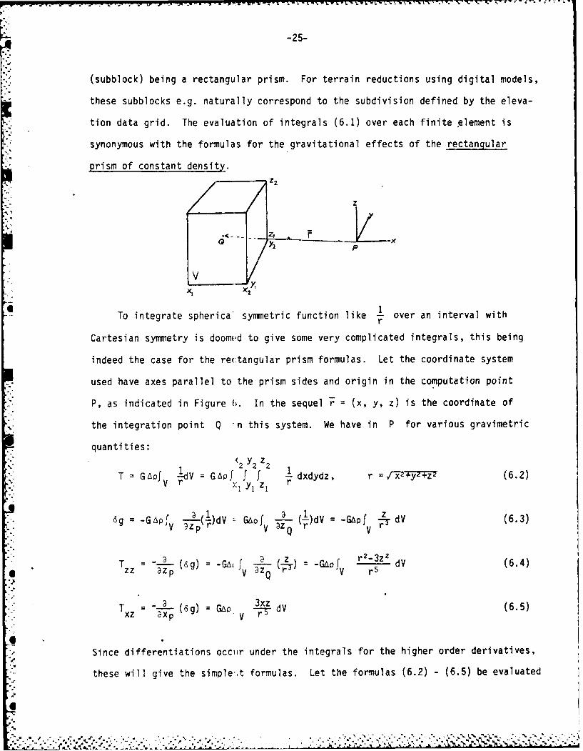
(subblock) being a rectangular prism. For terrain reductions using digital models,

these subblocks e.g. naturally correspond to the subdivision defined by the eleva-

tion data grid. The evaluation of integrals (6.1) over each finite element is

synonymous with the formulas for the gravitational effects of the rectangular

prism of constant density.

il zz

!1

,X, 2 ,

To integrate spherica symmetric function like - over an interval withr

Cartesian symmetry is doomed to give some very complicated integrals, this being

indeed the case for the rectangular prism formulas. Let the coordinate system

used have axes parallel to the prism sides and origin in the computation point

P, as indicated in Figure 0. In the sequel r = (x, y, z) is the coordinate of

the integration point Q n this system. We have in P for various gravimetric

quantities:<2 2 z 2

T = Gpfv V = GApf f f r dxdydz, r = 2 +y=-z (6.2); I Y 1 z I

6g 1- a ( )dv - f dV (6.3)V-: v

p 3rv v dV

S": Tzz - "..p L (cg) : ~ .G v . (.r) -G ofv r2-3Z2 dV (6.4)*zz 3 V QV r5

3xzT - " a -(6g) = GAo r- dV (6.5)xz 3Xp V

Since differentiations occur under the integrals for the higher order derivatives,

these will give the simple.t formulas. Let the formulas (6.2) - (6.5) be evaluated47

,

".'., .. ,. . , ; .- _,- .- .. . , . .- , .o . ... .. ... ,.. .- .- ..- -. , - -. , , .,,. ,,.,.-t-- ,.-.. ,'- ..-

-26-

as undefinite integrals to keep the notation simple. We have then for the second

order derivatives

T -GAP f f z dxdy =-GAz f 7y•z -dy GA z arctan (xr) (6.6)

z 1

T GA P f-z dxdy = GAP I -1 dy = GAP log (y+r) (6.7)-r y ryzY

For the first order derivative a non-trivial integration of (6.7) with respect

to x is obtained (Jung, 1961):

1

6g: -GAp f f - dxdy = GAp f log (y+r)dxrxy x

GAp(X log (y+r) + y log (x+r) - z arctan ( r)) (6.8)zr

Finally the formula for geoid undulations (height anomalies) are obtained by inte-

grating (6.8) with respect to z (MacMillan, 1958):

T: GAp[xy log (z+r) + xz log (y+r) + yz log (x+r)

(6.9)- arctan x.r- arctan -A- -2 arctan2 xr 2 yr 2 ta r~

The final formulas for the rectangular prisms are obtained by summing the

expressions (6.6) - (6.9) over the corners of the prisms with alternating signs,2 2 2

S()+j+k. 1 Z)e.g. T 1 k where Tijk is (6.9) evaluated at (x., y3 ,e1=1 (xi kk).

The formulas for the remaining derivatives (deflections of the vertical, other

second order gradients) are simply obtained by coordinate permutations, see Forsberg

and Tscherning (1981).

Although some simplifications of the final formulas are possible using addition

theorems for logarithms and arctan (arctana + arctanb = arctan a +-b the formulas

I-0

-27-

are still very complex and time consuming. In the terrain effect computa.tion

program (see appendix) an approximative formula, where the mass of the prism is

condensed as a mass layer on the xy-plane through the center of the prism, is

used for geoid undulations instead of (6.9). In this case we get an integral

similar to (6.8):

TGLp(z2 -zl) 1 dxdy

x y rzz(6.10)

GAp(z 2 -z I ) 1ix log (y+r) + y log (x+r) - Zmarctan Xy Ix2 Y2zmr x, yI

- z1+z2 rV:xy2+z

Zm 2 m

For terrain effect computations, this formuli has negligible error (typically

corresponding to millimeters in c).

In larger distances from the prism, the formulas (6.6) - (6.9) may be sub-

stituted by much simpler series expressions of the gravity field, obtained using

a spherical harmonic expansion of the prism field. Since the spherical harmonics

expressed in cartesian coordinates are simple homogeneous polynomials in x, y, and

z, the resulting series expansions are simple. In a prism-centered coordinate

system we have for the potential

T = GA p AxAyA z + + - [(2Ax 2 "Ay2-Az 2 )x 2 + (-Ax2+2Ay 2-Az2)y2

Ix y 1(6.11)+ (-AX2-Ay2+2AZ2)Z ] + 28--7 [a X4 + y + ... ] +

AX = x2 -x1 , Ay=y 2-y1 , AZ=Z 2 1

(MacMillan, 1958), from which gravity, second order derivatives etc. are easily

found by differentation. The first term in (6.11) is simply the point mass

approximation. The second term takes into account the different dimensions of

the prism - it is zero for a cube.

J-- s . --

-28-

In the terrain effect computation programme given in the appendix, a sub-

routine "PRISM" forms the nucleus of the calculations. This subroutine uses the

exact prism formulas when the computation point P is near the prism, in an inter-

mediate zone the MacMillan formula (6.11) is used, and finally in very large dis-

tances the point mass approximation is used. The shift between the formulas is

automatic, determined by accuracy levels wanted by the user. (cf. Figure 7).

It is through the additional use of the approximate formulas that the prism method

becomes feasible for "routine" gravity field modelling in mountainous areas, other-

wise evaluation of the complex exact prism formulas would often become prohibitive

in terms of computer time. Furthermore, in large distances the formulas (6.6)-(6.10)

become numerically unstable, requiring extended precision due to the differencing

of the evaluated "corner" - functions entering the formulas.

6.2 Frequency Domain

While the prism formulas are complicated in the s)ace domain, they are

surprisingly simple in the frequency domain. Since th? basics of Fourier analysis

of potential fields is not generally well known in geoJesy, a short

outline will be given first.

The Fourier spectral analysis is applied in the flat-earth approximation.

Let 7 be the reference plane (e.g. sea levef) with c)ordinates (x, y), and 7

the associated spectral plane with spatial frequencies (u, v). Then the Fourier

transformation is given by ("'" denotes transformed quintities):

T(u, v) f T(x, y)e' i(ux+vY)dxdy (6.12)

1 i(ux+vy)

T(x, y) =4- (u, v) dudv (6.13'

Upward continuation of the field to elevation z is obtained by a filtering

1(u, v, z) =T(u, v)e-wZ , Vu +v (6.14)

-29-

MAC MIL..AN GRAVITY POINT MASS

2%

61% 6S 5%

0 h 0 h

. p2"o / 2 .5s 2i

r, r

.2 .'.2

6- 6-V

1*4

4- 4-

2 - 2-

.2 .5 2

GEOI

6- S% 6-

4- 1 % 4-

2- 2 2-

0 hk 0 ,h

45 ' 2 .5 ' 2

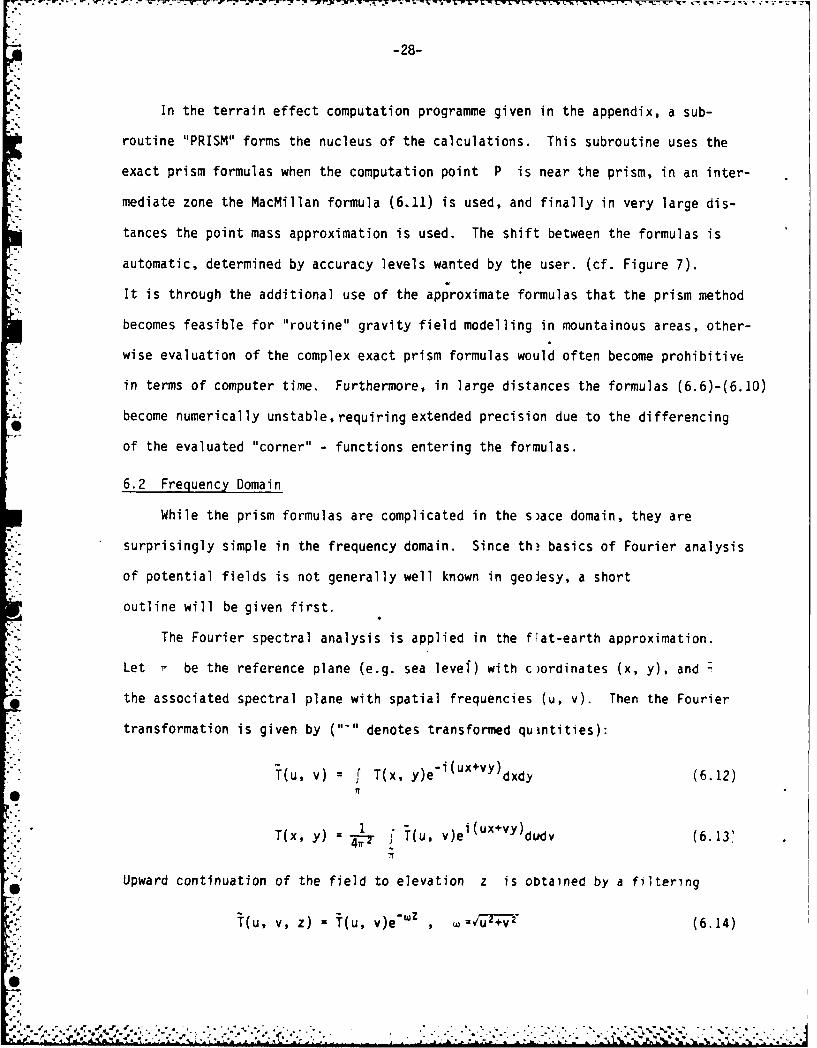
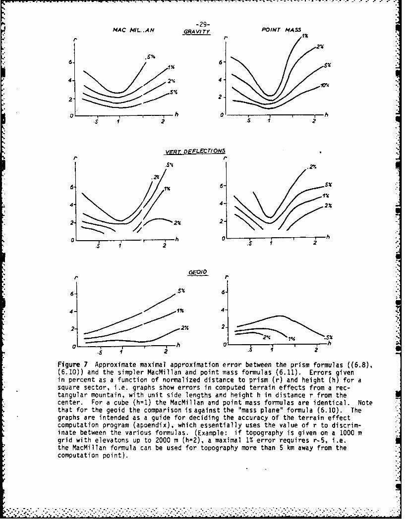
Figure 7 Approximate maximal approximation error between the prism formulas ((6.8),(6.10)) and the simpler MacMillan and point mass formulas (6.11). Errors given

in percent as a function of normalized distance to prism (r) and height (h) for asquare sector, i.e. graphs show errors in computed terrain effects from a rec-tangular mountain, with unit side lengths and height h in distance r from thecenter. For a cube (h=l) the MacMillan and point mass formulas are identical. Notethat for the geoid the comparison is against the "mass plane" formula (6.10). Thegraphs are intended as a guide for deciding the accuracy of the terrain effectcomputation program (apoendix), which essentially uses the value of r to discrim-inate between the various formulas. (Example: if topography is given on a 1000 mgrid with elevatons up to 2000 m (h=2), a maximal 1% error requires r-5, i.e.the MacMillan formula can be used for topography more than 5 km away from thecomputation point).

-30-

and similarly for the gravity field functionals (2.5)-(2.7) simple linear filters

transform the quantities in the spectral domain:

Z(u, v) .iv T(u v) (6.15)

(u, v) - T(u, v) (6.16)Y

Eg(u, v) = (-W- 2) T(u, v) -WT(u, v) (6.17)

where R in (6.17) is the radius of the earth.

For radial symmetric functions, f(x, y) = f(r'), r'= Ix7+y, the Fourier

transform (6.12) becomes a Hankel transform (Papoulis, 1968):

f(u, v) = 27rf(w) W= vu+v 2 (6.18)

where the Hankel transform pair (transform denoted by a bar) is given by:

f( ) = f r' f(r')j (wr') dr' (6.19)0 0

f(r') = fo ?(w) J0 (r') dw (6.20)

Here J (.) is the Bessel function of order zero. Of special importance is the

Hankel transform of the inverse distance:

1 _ 1 Hankel 1e-z (6.21)r vrr'+z W

(Papoulis, 1968, p. 145).

Now, for a rectangular prism (Figure 6), situated below the x-y plane, we have:01

T(x, y, 0) GAp dx'dy' dz' , (6.22)Vr

r : /(x-x') z + (y.y)Z + zZ

0'.-+

-31-

giving the transform

T(u, v) = Gp 1 -(uxvy) dx'dy'dz'dxdyVr

27r G6p f1 e -z' e-i(ux'+vY')dx'dy'dz,

11 Z2 -wZ l-i(ux+vy) Jx2 y 2 (6.23)27r GAP.e(-i) Ye (e -e6.x23)

Results for gravity and deflections may be obtained from (6.23) using (6.15)-(6.17)

and using (6.18) and (6.21) by interchanging the order of integration. Formulas

like (6.23) have been used for a number of years in geophysical exploration, especially

for the magnetic field (Bhattacharyya, 1964).

The advantage of the formula (6.23) is that it allows the use of the fast

fourier transform (FFT) when computing the gravity effects from a regular grid of

prisms, e.g. defined through a digital terrain model. If we have a set of nxm

prisms, the corners of the prisms, projected on the x-y plane, will form a

(n+1)x(m+1) grid mesh. By rearranging the sum (6.23) as sums over this grid, the

general expression for the total effect of all prisms will have the form

n+l m+1T(u, v) = f(w, xj, Yk)e-i(uxj+vY k) (6.24)

j=1 k=1

where f contains sums and differences of e" z for the prisms adjoining the grid

point (xj, yk). Sums like (6.24) is exactly what is obtained by the FFT algorithm -

had it not been for the dependence of f with w. This dependence is due to the

basic fact that the prism integral (6.22) is fundamentally unlinear, not being a

convolution. We are thus forced to evaluate (6.24) on a frequency-by-frequency

basis by FFT, for each value of w a separate spectrum T is obtained and the

final spectrum must then be "constructed" by carefuly selection and interpolation

in this set of spectra. The thus obtained final spectrum may then be transformed

back into the space domain by an inverse FFT.

0L

-32-

It is important to stress, that (6.24) is exact. Therefore the spectral

values obtained using (6.24) are not influenced by window effects etc., the ob-

tained spectrum represents the spectrum of a transient signal, this ignal decreasing

quickly to zero outside the area covered by the prisms. The only "errors" occurring

in this FFT technique is in the w-interpolation scheme to obtain the final spectrum,

and in the final synthesis of the frequencies, since FFT only gives the sums (6.24)

for a finite, discrete number of frequencies, the highest frequencies being the

Nyq~ist frequencies for the prism grid. This secures, however, a nice smoothness

of the computed field, since e.g. a representation of the topography with flat-

topped prisms is anyway a rather poor representation, causing unwanted high frequency

spectral "ripple" effects from the edges.

To estimate the gain in computing speed, consider as an example a nxm grid

of prisms (with varying top and base levels), and assume we want to compute the

gravitational effects in the same grid at a fixed altitude. Then the operations

will be (orders of magnitude):

SPACE DOMAIN: n xn2 calls of "PRISM" subroutine (no computation-saving grid symmetries exists for 'exact" formulas)

FREQUENCY DOMAIN: n/2 spectra (6.24) of n2 coefficients f,FFT speed nlogN, spectral selection, inverse FFT.Combined order of magnitude: n3logN

The gain is thus moderate, a consequence of the unlinearity of (6.22).

A real significant gain in computation speed is obtained if the basic volume

integral (6.1) is approximated with surface convolution integrals. Inis is

e.g possible for "thin" prism layers at near constant depth, and to some degree

also for terrain effects (so-called "linear topographic approximation"), involving

integrals of the topographic elevations and their squares (more details in next

section). In the case of a "thin layer" at average depth D, we obtain

*

.. . . . . . . . . .

. . .

-33-

T(x, y, 0) = G A -p dx'dy'dz'Vr

V

G f (x, dx'dy' (6.25)SG [(x-x, )'+(y-y, )'+D2] 6.25

where K :Ao (z2-z,) is the surface density. The transform is obtained simply

by utilizing (6.21) again, giving

T(u, v) = 21rG- e - D i (u, v) (6.26)

In this case the order-of-magnitude computation speed of the previous example

will be only n2logn if FFT is utilized, but opposed to the "exact" spectral formu-

lation "window effects" due to finite data lengths must.now be given full attention.

The frequency domain methods have as common restrictions that data and compu-

tation points must be 'n a grid, the computation points being in a plane (im-

portant exception: grivimetric terrain corrections, cf. next section). Obvious

applications could be e.g. for geoid computations at sea level (especially for

satellite altimetry) and upward continuation studies iairborne gravimetry and

gradiometry). The importance of spectral methods in (qeophysical inversion may

be inferred from (6.26): if a particular spectrum (e.g. white noise) is expected

for the source K, then the depth D to the sour:e may be found directly from

the observed gravity field spectrum. This is the base of the widespread "statis-

tical inversion techniques", dominating in the analysis of aeromagnetic data.

7. Terrain Reductions

For the remainder of this report, emphasis will now concentrate on topo-

graphic and isostatic reductions - a synonym for computational elimination of

the effects of the two most dominant and best known density anomalies of the earth:

the visible topography and its associated compensation at depth. For such gravity

field effects the general term "terrain effects" will be used in the present context.

:i. .'/ :.' -. ..,..--,-.. .- > -. i -i .> -i . - . > . ... > . i ... ' - - .".' ..- , ~ . i .> ,- -- - ..- ..

41

-34-

The commonly applied term "terrain corrections" will he reserved for the narrow

meaning, i.e. a correction to the Bouguer reduction, to give the true (unlinear)

effect of the topography on gravity anomalies (and deflections of the vertical

as well).

7.1 Terrain Effects and Associated Density Anomalies

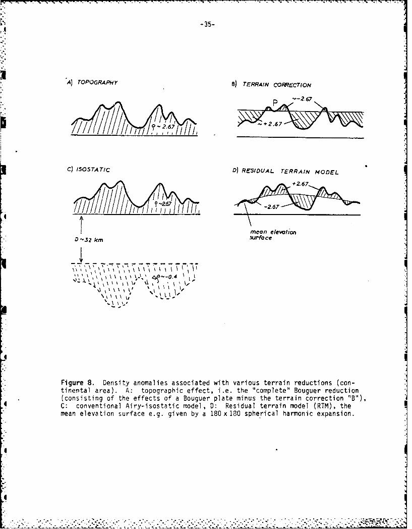
The various terrain reductions in use is illustr ted in Figure 8. To use

terrain reduced data in a "remove-restore" technique for gravity field modelling

(Section 4), it should be remembered that the density models indicated by Figure

8 should either cover a given, fixed geographical area, or - or at least in prin-

ciple -.be global.

The topographic reduction or complete Bouguer reduction consists of removing

the visible topography. Conventionally a density of 2.67 g/cm3 is used. This

density, which represents a typical density of granite and many Paleozoic and

Pre-Cambrian sediments, is fairly good in mountainous areas. However, one should

not hesitate to use other density values, since the density may range from below

2.0 g/cm3 in moraine hills to 3.0 g/cm 3 in volcanics. Average density values

could be chosen from geological considerations or usirg the inversion techniques

of the last section. At the oceans the topographic dEnsity anomalies are formally

negative, the standard density 2.67 corresponding to 1.03-2.67= -1.64 g/cm 3, 1.03

being the density of sea water.

The topographic reduction may formally be split into a Bouguer term, the

effect of an infinite plate, plus the terrain correction, which takes into account

the topographic irregularities. For gravity disturbanzes we have

2r G hp - tc (7.1)

where 2-Gohp is the gravity due to a (plane) Bouguer plate of thickness hp

(if the computation point P is situated above the topography, hp is the topo-

graphic elevation at the surface point below P), and tc is the terrain correction.

0 i' -.i ' ' I L> -- -1. L . i.> - - '' 11? .- .. " - " -" ' ] L1 .L, > "

-35-

A) TOPOGRAPHY a) TERRAIN CORECTION

P-267

/67 / 2/.67~

C) 1505TATIC D) RESIDUAL TERRAIN MODEL

mean elevotion"32 km .urface

4? 4

Il

Figure 8. Density anomalies associated with various terrain reductions (con-tinental area). A: topographic effect, i.e. the "complete" Bouguer reduction(consisting of the effects of a Bouguer plate minus the terrain correction "B"),C: conventional Airy-isostatic model, 0: Residual terrain model (RTM), themean elevation surface e.g. given by a 180x180 sphe.rical harmonic expansion.

I,

4J

-36-

The terrain correction is always positive (in the plane approximation) due to

the conventional minus sign in (7.1).

For deflections of the vertical the terrain correction and the topographic

effect are identical (except the signs), since the Bouguer plate effect is zero.

For height anomalies, however, the infinite Bouguer plane can not be used, the

effect being infinite. Instead one could think of using a spherical Bouguer plate:

the effects typically computed, will however, still be very large and often much

larger than the observed geoid undulations themselves (on a global basis). Topo-

graphic reductions are therefore not very applicable to general gravity field

modelling: the large model geoid effects and biased Bouguer anomalies at oceans

and mnuntainous areas necessitates some kind of negative density anomalies being

introduced, e.g through an isostatic compensation hypothesis. Needless to say,

the topographic reduction is naturally very well suited for problems such as gravity

interpolation and geophysical inversion.

Isostatic reduction formalizes the prevailing tendency of the earths topo-

graphy to be compensated at depth. The standard Airy scheme assumes local compen-

sation through a root system (Figure 8D), the thickness of the root being

t = -Lh 6.7 h (7.2)

AP

where o is the density of the topography (-2.67 g/ci 3) and Ao the density

contrast between the crust and the mantle (-0.4 g/cml). The normal density model

has a crust of thickness D (-32 km).

Naturally the earth does not fully follow this simple principle. Although

(7.2) approximates the overall isostatic compensation fairly good, many exceptions

occur: first of all the strength of the earth's crust supports short-wavelength

topographic features, isostasy being primarily a regional phenomena. Second,

many regions are either uncompensated or compensated at deeper levels (through

,.. .. .2 .-.-.-. -,. '-.' .'.. + ' . - . . ... . " - . ' ." , . ... .. ,. . ,.- *.*. , .. ,.-. -. . .. '.-.,- •

-37-

anomalous density values in the upper mantle),most noticeably the deep-sea trenches

and mid-oceanic ridges. However, since the computed isostatic effects are very

insensitive to the actual isostatic formulation and parameters used, even the

simplest formulations (e.g. (7-2)) gives excellent results, the results being "good"

when the remaining field after isostatic reduction is smooth and with low variance.

Global isostatic reductions attain maximal values for the geoid in the range 10-20 m.

It is therefore necessary to compute isostatic effects also on spherical harmonic

coefficients .for the geopotential, e.g. using the simple formula (3.12).

A drawback of the isostatic reduction is that it primarily should be global.

If only a fixed, localized area is taken into account, the computed isostatic

gravity field effects will be influenced by "edge effects": the computed isostatic

gravity and deflections of vertical would change rapidly near the boundary for

non-zero elevations. For the geoid an overall bias, dependent on the chosen size

of the reduction area, will result if the area mean elevation is different from

zero (see e.g. Forsberg & -scherning, 1981, Figure I).

Since the main problem in external gravity field modelling in mountainous

areas is short-wavelength topographic "gravity field noise", a terrain reduction

method avoiding the "global" computations of isostatic reductions, but capable

of approximating isostatic conditions, would be ideal:

For a residual terrain model (RTM) reduction only the short wavelength

of the topography is taken into account. This is done by choosing a smooth mean

elevation surface, and computationally remove masses above this surface and fill

up valleys below (Figure 8D). The mean elevation surface could be any smooth

surface, representing mean elevations of the area, e.g. an interpolation in 30'x30'

mean heights or - especially - defined through a high-order spherical harmonic

expansion of the topography of the earth. In this case the RTM density anomalies

correspond to a normal density distribution (normal earth) with smooth topography

and bathymetry defined through the spherical harmonic expansion, and thus

4

0-38-

corresponds to the residual gravity field after removal of a similar spherical

harmonic expansion of the geopotential.

The advantages of the RTM-reduction are many: s-nce the density anomalies

hgve oscillating positive and negative values, the inlegrations for gravity field

effects need only be done out to some suitable distan(e from the computation point,

the influence of distant topography cancelling out. ilso, terrain effects on

height anomalies will be small (often negligible if a short-wavelength reference

elevation surface is chosen), and especially for e.g. 180x180 height expansions

the reduction gives results close to isostatic reductions.

The similarity between RTM and isostatic reducti(.ns are analogous to the

similarity between mean free-air gravity anomalies ana isostatic anomalies.

Indeed, by a special choice of mean elevation surface nearly complete correspon-

dence may be obtained: If we define the mean elevations through the low-pass

filter (plane approximation)

href(P) =_- _ d -[ h dQ r = dist (P, Q) (7.3)ref[r2+D21]/2 'Q

then Moritz has shown that the associated RTM-reduction corresponds to an

isostatic reduction with a (surface layer) compensation depth D (Moritz, 1968a).

Note that (7.3) is nothing but the well-known Poisson integral for upward con-

tinuation of harmonic functions.

The RTM-reduction may be viewed as a difference between two Bouguer reductions:

first the visible topography is removed, and then the smoothed topography is added

back (Figure 9):

L(T)RTM : L(T)TOPO - L(T)REF TOPO (7.4)

Each term in (7.4) may formally be split in a Bouguer plate effect and a terrain

correction. Table 1 shows sample terrain corrections for a 180 x180 spherical

harmonic reference surface in two 40x40 fixed areas in tne Rocky Mountains.

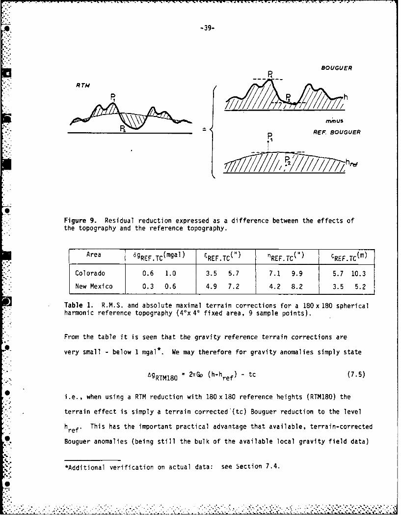
-39-

BOUGUER

R TM

minus

p REF BOUGUER

Figure 9. Residual reduction expressed as a difference between the effects ofthe topography and the reference topography.

Area gREF. (mgal) REF.TC REF. TC REF. Tc(m)

Colorado 0.6 1.0 3.5 5.7 7.1 9.9 5.7 10.3

New Mexico 0.3 0.6 4.9 7.2 4.2 8.2 3.5 5.2

Table 1. R.M.S. and absolute maximal terrain corrections for a 180x180 sphericalharmonic reference topography (40x4' fixed area, 9 sample points).

From the table it is seen that the gravity reference terrain corrections are

very small - below 1 mgal*. We may therefore for gravity anomalies simply state

'gRTM180 2TrGp (h-hr) - tc (7.5)

ref t

i.e., when using a RTM reduction with 180x180 reference heights (RTM180) the

terrain effect is simply a terrain corrected (tc) Bouguer reduction to the level

href . This has the important practical advantage that available, terrain-corrected

Bouguer anomalies (being still the bulk of the available local gravity field data)

*Additional verification on actual data: see Section 7.4.

... -. ...0-. .. . .. .. , .. -: . . - . .. ... ; , .,.. , - -, .,. . ." ' . . , ," " ", ,''" , ,-- - ", ,

-40-

may be applied directly for RTM-reduction using (7.5). For deflections of

the vertical, however, the time-consuming "prism"-integrations can not be avoided,

the deflection terrain effects due to the changing reference level being much

too large.

When performing the RTM-reduction "directly" (e.g. using rectangular prism

integration), stations above the reference level are left "hanging in the air",

while observations below this level are reduced to their values inside the mass

(Figure 9). However, for external gravity field modelling, we need not the value

inside the mass, but the harmonically downward continued value, corresponding

to the outer, "reduced" field. In other words, what would the reduced observation

be at the point P2 in Figure 9, if we treated the mean topography as non-existent?

An approximate answer to this question is simple: if the density above

a plane through P2 is condensed in a mass plane layer immediately below P2 .

deflections of the vertical and geoid undulations would remain nearly unchanged

due to the smooth, low-slope reference surface. For gravity anomalies, however,

we would see a change

c C- m 47r GAh (7.6)' gharmonic 6gin mass

corresponding to a "double" Bouguer reduction with plate thickness 1h = h - href P*This "harmonic correction" must be applied for all gravity stations below the

reference level when "direct" prism integration of RTM density anomalies (Figure

8D) is performed. If instead (7.5) is used, the correction is taken into account

"implicitly".0

7.2 Practical Terrain Reductions in Gravity Field Modelling

A FORTRAN 77 program for computation of any of thi four types of terrain

effects (and corrections) mentioned (Figure 8) are listed in the appendix.

0

". " -. ""' J . - '' ' , '" ' - " ," / "% ' , "° .*p".. . .'"-.-." = '' % ." ."-", -" '' ' - " ," ,"

6-41-

The program uses rectangular prisms for a direct integration of geoid undulations,

deflections of the vertical or gravity anomalies from digital terrain models given

on a geographic grid.

Special precautions have been taken to evaluate the inner zone effect, i.e.

the influence of the topography adjacent (say, within I km) to the computation

point. These inner zone effects may be very large, especially for gravity terrain

corrections. To re'present the inner zone, a bicubic spline interpolation of the

topography is utilized. However, since gravity topographic effects to first order

depends linearly on the gravity station elevation, it is clear that the station

elevation itself should be utilized in the inner zone interpolation. An option

in the program allows the height interpolation procedure to give the correct eleva-

tion at a station,through a smooth "adjustment" of the digitial terrain model

elevations in the inner zone. For deflections and height anomalies, where the

station height dependence is weak, use of this option is not necessary.

Actual examples of use of the various terrain reductions in connection with

gravity field modelling by collocation can be found in e.g. Forsberg and Tscherning

(1981). Here gravity and deflections were modelled with an accuracy around 4mgal

ana 1" respectively, in a mountainous area (New Mexico), using gravity data spaced

c. 6' apart and a 0.5'.x0.5' digital terrain model. When applied properly, nearly

the same results were obtained for all types of terrain reductions.

As an outline example, let us consider upward continuation of gravity data

in a mountainous area. Using a "spatial" modelling technique like collocation

or point mass modelling the application of the remove-restore technique for

a RTM180-reduction (and a 180x 180 reference field) is simple:

1. Compute terrain corrections for local gravity stations if not already given.

2. Obtain terrain-reduced residual gravity values by subtracting thereference Bouguer anomalies AgREF - 27GohREF from the local, terrain-corrected Bouguer anomalies.

3. Apply upward continuation method,

4. Add back RTM-effects computed at altitude (prism integration),

5. Add back 180x 180 gravity computed at altitude.

•6 " - - - , " " " ' ' ' " ' . . ' ' ' " ' o ' " ' ' ' . , ' " ' . ' .. -.-' ' - -. . .' -. . " - - -i '

9-42-

For already gridded gravity data (e.g. 5'x 5' mean free-air anomalies) this

remove-restore technique may be used with some caution. For a mean block we would

need the mean terrain correction, as we have from (7.5)

gRTM180 2Gp ( - hREF) - t (7.7)

Such mean terrain corrections tcE are difficult to estimate. They are,

however, very important since they play an essential role in the harmonic down-

ward continuation of gravity data from the surface of the topography to the geoid,

a necessary prerequisite for the application of e.g. the classical integral meLhods.

Apart from direct computation of tc by averaging, its magnitude may be estimated

from the covariance function of the topography

C2tc 3 Gp d

where a2 is the terrain variance and d the correlation length, as pointedh

out by Sunkel (1981a).

7.3 The Linear Approximation for Topographic Effects

Approximate formulas for RTM-effects, especially applicable for error studies

and frequency domain methods, may be obtained using functional expansions of the1 z

topographic volume integral kernels (I , .- T etc.). In the sequel a "long wave-

length" reference elevation surface e.g. 180 x 180 spherical harmonic expansion

is assumed to be used.

In the plane approximation we have for the RTM potential effect when a con-

0 stant topographic density is used:

h

T= G f A-dV= G f f dzd, (7.8)m r rz~href

where

0

-43-

1 [r +- (z-h) 2 ] [1 + tan2B] " (7.9)

r o ro r00 0 00

V is the volume of non-zero (positive or negative) density anomalies Ao, shown

hatched in Figure 10. A series expansion for Tm is obtained by expanding (7.9)

hphref

.. .. .. h h

r Isea /eve/

101

Figure 10

with respect to the inclination s, which is always small except for the inner

zone in rugged topography (and geoid innerzone effects are very small). Thus,

1 1 1 (z - hnp) 21 1 - I( ) + (7.10)r r 0 2 r03

and by inserting (7.10) in (7.8) and integrating with respect to z

Tm = Go f h - href dr 1G f (h - hp)P - (href -hp) 3 dr + (7.11)4 m=~f r0 di- r3 d "" .. 7.1

1! 6 IT r3ro 0

The first term in (7.11) has been called the linear approximation by Moritz (1968a).

It is seen that this term represents nothing but the potential of a mass coating

p(h - href) = pAh. Within the accuracy of the linear approximation we may

view this mass coating as a surface density layer at the height reference surface.

The higher order terms in (7.11) may similarly be viewed as successive coatings

of dipoles, quadropoles, etc.

- . .. . .. . --.-b

0 -44-

For deflections of the vertical we have

h fcos a2:J=-* y{:z &dV='i fi f dz dir(712PIhreF il

which by expansion r-3 =rj3

-- *r65 (z -hp) 2 + .. and integration analogous

to the potential case gives

Em(h-href) {Cosa 1 a hh) 3 -(hrefhp)

3 Cosa 4 di

fm jY r sin a 2 r~ 4sina iJ

(7.13)

Aqain, the first term (the linear approximation) may be interpreted as the effect

of a mass coating.

The RTM gravity anomalies are given by

h z-h T( .4

Tr zhrefR

The last term in (7.14) -the indirect effect - ill usually be below 1 mgal

for a 180 x 180 reference surface and may be neglec ed. For gravity anomalies

*it is advantageous to use (7.5)

Ag 27tGr, (h -href) -tc (7.15)

*and then only expand the terrain correction

h (7.16tc=Gpj P zf (.6zh~ r3

(h -p P~ dir +.. (7.17)

20r

-45-

In (7.15) the Bouguer term is on the average one order of magnitude larger than

the terrain corrections themselves. In some cases -e.g. error studies - it would

therefore be sufficient only to use this simple term. For gravity field modelling

with heterogeneous data it is, however, very dangerous not to include the best

possible terrain corrections: since tc is always positive, a systematic bias

will be introduced in tgm, a bias which often would seriously affect computed

geoid undulations.

For frequency domain formulas we note, that the linear approximations in

(7.11) and (7.13) are convolutions, i.e. expressions of the form

L(Tm)p = k*Ah k(xp-XQ, yp-yQ) Ah (XQ, yQ)drQ (7.18)IT

and thus in principle for the Fourier transform using the well-known convolution

theorem

L(T) = k Ah (7.19)

The function k is traditionally called the impulse response, K the transfer

function. Ah = h-href will be termed the residual height hereafter.

For the potential we have from (6.26)

(u, v) 21Go 1 Ah (u, v) , u +V7 (7.20)m

and since (also) in the linear approximation Em = "--l 2m we haveY ay

jm (u, v) = 17G-~h(,v)(.1

and by (7.15)

Aim(u, v) = 21TGp A h (u, v) - tc (u, v) (7.22)O

0%

.. . * *.'..

-. . . . . . . .

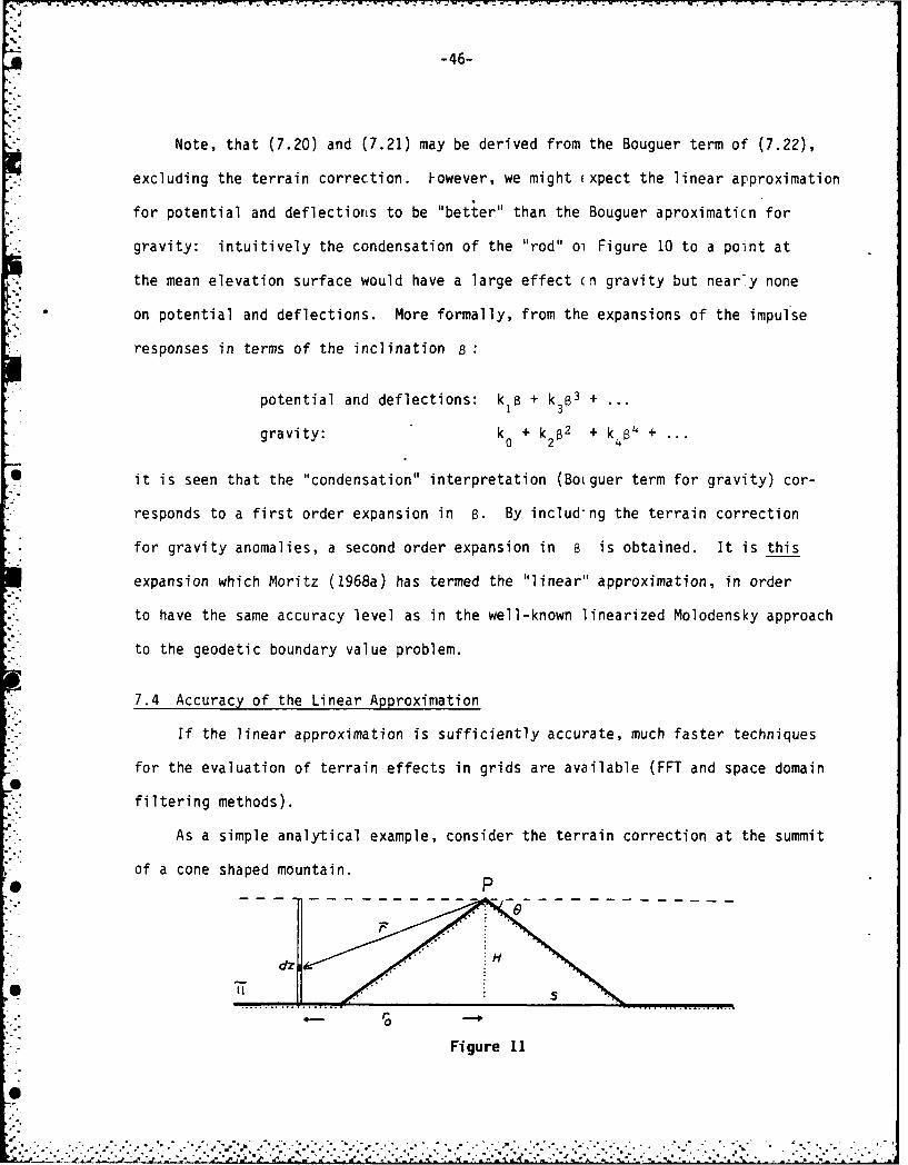
-46-

Note, that (7.20) and (7.21) may be derived from the Bouguer term of (7.22),

excluding the terrain correction. Fowever, we might (xpect the linear approximation

for potential and deflectiorns to be "better" than the Bouguer aproximaticn for

gravity: intuitively the condensation of the "rod" ol Figure 10 to a point at

the mean elevation surface would have a large effect (n gravity but nearly none

* on potential and deflections. More formally, from the expansions of the impulse

responses in terms of the inclination B:

potential and deflections: kIB + k 3B3 +

gravity: k0 + k 2B2 + k4B 4

+

it is seen that the "condensation" interpretation (Botguer term for gravity) cor-

responds to a first order expansion in s. By includ'ng the terrain correction

for gravity anomalies, a second order expansion in B is obtained. It is this

expansion which Moritz (1968a) has termed the "linear" approximation, in order

to have the same accuracy level as in the well-known linearized Molodensky approach

to the geodetic boundary value problem.

7.4 Accuracy of the Linear Approximation

If the linear approximation is sufficiently accurate, much faster techniques

for the evaluation of terrain effects in grids are available (FFT and space domain

filtering methods).

As a simple analytical example, consider the terrain correction at the summit

of a cone shaped mountain.Pdfl ... O--------

dZ

• I .. .... .... ..... ,./. ................. ..

Figure 11

.......................

S,.° °.. . . . .,. °.. . . .,l . o.°... • . ..-. U * *". . . .* . ,

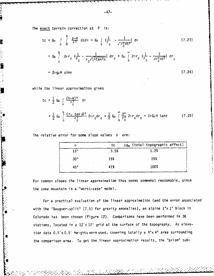
-47-

The exact terrain correction at P is:

h z-H 1 1

tc = Go f f -r- dzdr= Go f 1( dr (7.23)H r o

-Go f 2rr ( )dr + Go f 2rr ( -- -)dr0 r r0 1+tane 0 r2+H2

00 r0 /ItnoS0 0

S2TrgpH sine (7.24)

while the linear approximation gives

tc 2± Gp J (h4L dir7T 0

1 Go (r, tan e2 2rrr 0 +1 H2SGo r (r, tanG 2 2rr dr 2TrGpH tane (7.25)S0 050

The relative error for some slope values e are:

e tc Agm (total topographic effect)

150 3.5% 1.2%

300 15% 15%

450 41% 100%

For common slopes the linear approximation thus seems somewhat reasonable, since

the cone mountain is a "worst-case" model.

For a practical evaluation of the linear approximation (and the error associated

with the "Bouguer-split" (7.5) for gravity anomalies), an alpine 10x 10 block in

Colorado has been chosen (Figure 12). Comparisons have been performed in 36

stations, located in a 12'x 12' grid at the surface of the topography. As eleva-

tion data 0.5'xO.5' heights were used, covering totally a 4°x4' area surrounding

the comparison area. To get the linear approximation results, the "prism" sub-

6

.................. ~ -

-48-.4 LON~iTUDE

2 5 3 2 5

40

c /, J>~

N C()~ ? N

NA

4 N'

C ~ -~\ ~~N> N K-

~~k\2

35 25qFigure 12 Rok onants raue o vla no h lna prx i

imaton" Thej~Z II 8 m ratpgrpysonw hacntu nevlo 0c nore fro I' 'ma egt. Tehget on t let 39m

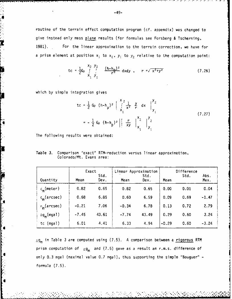
*~~~~~~~ T .. C . - . -7

-49-

routine of the terrain effect computation program (cf. appendix) was changed to

give instead only mass plane results (for formulas see Forsberg & Tscherning,

1981). For the linear approximation to the terrain correction, we have for

a prism element at position x, to x2, YI to Y2 relative to the computation point:

I_ X2 Y2 (hh)2 2ytc 1 Ir2 __h-h_

x - r r= x2+y2 (7.26)xI Yi

which by simple integration gives

XI 2 Y2tc Gp (h-h )2 dx y(7.27)

x y2 Gp (h-h p)2 r I 2

2

The following results were obtained:

Table 3. Comparison "exact" RTM-reduction versus linear approximation,Colorado/Mt. Evans area:

Exact Linear Approximation DifferenceStd. Std. Std. Abs.

Quantity Mean Dev. Mean Dev. Mean Max.

Cm(meter) 0.82 0.65 0.82 0.65 0.00 0.01 0.04

Km(arcsec) 0.68 6.85 0.60 6.59 0.09 0.69 -1.47

nm(arcsec) -0.21 7.06 -0.34 6.78 0.13 0.72 2.79

Agm (mgal) -7.45 43.61 -7.74 43.49 0.29 0.60 3.24

tc (mgal) 6.01 4.41 6.33 4.94 -0.29 0.60 -3.24

Ag in Table 3 are computed using (7.5). A comparison between a rigorous RTMm

prism computation of Agm and (7.5) gave as a result an r.m.s. difference of

only 0.3 mgal (maximal value 0.7 mgal), thus supporting the simple "Bouguer" -

formula (7.5).

• -, . . .. - . - . .. -. .- . , . . .. . . . - . . . . . . , - -. , - , , -•...-., . ..* *-

-50-

From Table 3 it is seen that the linear approximation errors are insignificant

for geoid undulations and also rather small on the average for gravity, but with

a possibility for rather large outliers. For deflections the error might not

always be acceptable, and higher order expansions might be necessary. Considering

the extreme ruggedness of the test area, other "milder" areas will be expected

to give better results, and certainly the linear approximation will always be

very useful since it allows the use of FFT methods for terrain effect computations.

7.5 The Terrain Correction as Convolution Integrals

From (7.17) we have in the linear approximation

tc = Gp j (hh3)2 d7 (7.28)Tr r3

0

which may be expressed as convolutions of h and h2:

tc = Gp[ - d + hd - -2h4 d] (7.29)7T r3 T r 3 r:~ 0 ~ 0 TTr

since hp is constant with respect to the integration, we obtain

tc = Gp [(h2*f) + h' f dr - 2h (h*f)] (7.30)p p

wheref- 1 Now, the function f does not have a fourier spectrum,(X2+y2 )3/2

i

but it may be regularized very simply: Instead of f consider f' -(x2+y2+a

2 ) /2

where a is a small constant. Using f' instead of f as kernel in (7.28), this

corresponds to a computational upward continuation to a distance a, and when

a is chosen sufficiently small the error will be insignificant and only affect

* an innerzone roughly of radius a. We thus have:

tc zGp [(h2*f' + 2h2 - 2h (h*f')] (7.31)

a p p

where the center integral of (7.30) has been evaluated analytically (the integral

is nothing but the well-known Bouguer-plate integral).

S

.. . . . . . . . .

-51-

The two convolutions in (7.31) may with advantage be evaluated using fre-

quency domain methods, we have e.g.

transform of (h2,f') 2 2 . _ 2. e- a 12 (7.32)a

see Papoulis (1968), p. 145. With the split of the terrain correction (7.31)

it is clear, that for practical applications there will be a lower limit for a",

since the terrain correction is expressed as a (small) difference between two

large numbers, and thus unstable numerically.

Since "a" can not be chosen arbitrarily small, a small error Atc is made,

by using integral kernel f' instead of f, rEpresenting the "suppressed" effect

of the local innerzone just around the computation point. If the regularization

distance "a" is chosen somewhat smaller than the finest resolution of the given

elevation data, a quantitative estimate of tiis "regularization error" Atc may

be obtained as follows: The error is

Atc = Gpf ((h-hP)2 -r 2:(-h). ) dr (7.33)

r0 0r- aj /

Since this error is dominated by a very local innerzone effect, a Taylor expansion

of the topography is adequate, keeping only the first terms to represent a sloping

plane. Then by assuming the computation point to be at origo we hiave

(h-h )2 ro2 tan 2e Cos 2a (7.34)

p 0

where e is the slope of the plane and e the azimuth from the direction of

maximal slope. Insertion of (7.34) into (7.33) gives

0 2 r 0r o 2, t n 2 r 2 t a n o1 tc = h2GO r )- (r u ar

2 r3 r2+ a 2]/V2 00 0

r2

= JrGo tan 2e r (1 rr+a2)/) dr0 (7.35)0

0 0

-52-

This integral may be tackled by substitution of r2 , giving0

2

Atc -k2rGp tan2e r0 ro+2a2

0 0

= rGp tan2ea (7.36)

This is exactly the (linear approximation) terrair: correction of a sloping innerzone

of radius 2a (it is evident from (7.34) that this te-rain correction must be half

the corresponding cone terrain correction (7.25)). A nuii,.rical example: if a = 100 m

and e = 300, the regularization error will be 1.8 mgal. This illustrates the

critical importance of the very local station surroundings for gravity terrain

corrections, and the fact that "a" can not be chosen too large - reasonable values

must be chosen based on empirical investigations.

7.6 The Use of FFT for Terrain Effect Computations

In the previous sections frequency-domain formulas for terrain effects on

height anomalies, deflections of the vertical and gravity anomalies have been

discussed. These expressions are very useful since digital terrain models are

naturally given in grids, suitable for direct use of the Fast Fourier Transform

(FFT). The speed of FFT (-nlog 2n if the number .of points n is a power of 2,

otherwise somewhat slower depending on the prime factorization of n) certainly

makes the application of frequency domain methods attractive especially when large

volumes of dataineed to be terrain reduced. However, before applying the

method, it is essential to realize the limitations inherent when using FFT.

FFT is basically a fast algorithm to determine the discrete transform of

periodic data. The two-dimensional discrete Fourier transform pair may be expressed as

n-1 m-1 P qkh(pAu, q~v) AxAy h (jAx, kAy)e " ( n m (7.37)nm j=0 k=0

4

45 * -~*.* . , * .

-53-

- n- - p , ak.n-jAm, k1y) - h(pAu, qAv)e27r n m (7.38)

h ,ky-Axy p:O q=O

where Ax and Ay are gridspacing in the given elevation grid of nxm points,

and the normalization factors have been chosen to be in accordance with the con-

tinuous transform (6.12-6.13). The frequency spacings are given by

2Tr - rA- AV MAY (7.39)

The spectrum h as well as the original data h must be viewed as infinitely

periodically extended in space. Since the Nyquist frequencies

uN - Au Av A y (7.40)2 AX' vN Ay

represent the highest frequencies obtainable from the gridded data, frequencies

above (uN, vN) in (7.37) will correspond to negative frequencies. For more details

on FFT see e.g. Kanasewich (1975).

When applying FFT for convolutions of the form (7.18) or (7.31), the periodic

extension means that for a data point near an edge, the convolution will actually

"use" data from around the opposite edge as well. The convolution kernel will

in effect be truncated (and periodically extended) when applying the analytical

terrain effect filters at the discrete frequencies of the FFT (Figure 13), and

this means in common words that the terrain effects computed using the FFT method

will be terrain effects from a "running area" of size (nAx, mAy), centered at the

computation point. At the center point of the grid the computed effect will

exactly be the effect of the given area - at a corner point the result will be

completely erroneous, since 3 of the 4 quadrants around the corner will be integrated

with the "non-existent" periodically extended heights.

"

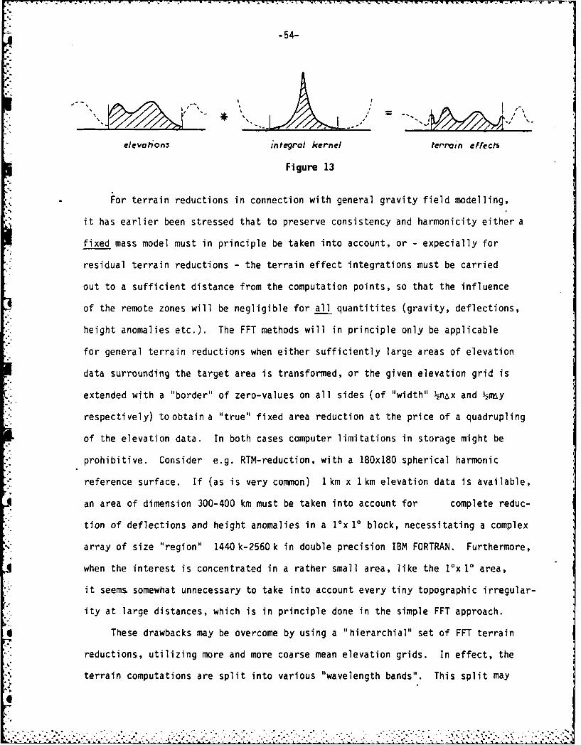
-54-

elevahons tntegral kernel terrain effects

Figure 13

For terrain reductions in connection with general gravity field modelling,

it has earlier been stressed that to preserve consistency and harmonicity either a

fixed mass model must in principle be taken into account, or - expecially for

residual terrain reductions - the terrain effect integrations must be carried

out to a sufficient distance from the computation points, so that the influence

of the remote zones will be negligible for all quantitites (gravity, deflections,

height anomalies etc.). The FFT methods will in principle only be applicable

for general terrain reductions when either sufficiently large areas of elevation

data surrounding the target area is transformed, or the given elevation grid is

extended with a "border" of zero-values on all sides (of "width" nAx and m~y

respectively) to obtain a "true" fixed area reduction at the price of a quadrupling

of the elevation data. In both cases computer limitations in storage might be

prohibitive. Consider e.g. RTM-reduction, with a 180x180 spherical harmonic

reference surface. If (as is very common) 1km x 1km elevation data is available,

an area of dimension 300-400 km must be taken into account for complete reduc-

tion of deflections and height anomalies in a ixi1 block, necessitating a complex

array of size "region" 1440k-2560k in double precision IBM FORTRAN. Furthermore,

when the interest is concentrated in a rather small area, like the 1ixi* area,

it seems. somewhat unnecessary to take into account every tiny topographic irregular-

ity at large distances, which is in principle done in the simple FFT approach.

These drawbacks may be overcome by using a "hierarchial" set of FFT terrain

reductions, utilizing more and more coarse mean elevation grids. In effect, the

terrain computations are split into various "wavelength bands". This split may

. , . . % ." . . .- . .' .. . . '. ' - .- . . . * . .)- , - .. . .. . . . ., .

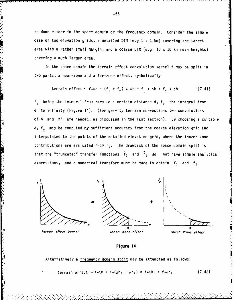
-55-

be done either in the space domain or the frequency domain. Consider the simple

case of two elevation grids, a detailed DTM (e.g 1 x 1 km) covering the target

area with a rather small margin, and a coarse DTM (e.g. 10 x 10 km mean heights)

covering a much larger area.

In the space domain the terrain effect convolution kernel f may be split in

two parts, a near-zone and a far-zone effect, symbolically

terrain effect - f*Ah = (f + f) * Ah = f* Ah + f., *Ah "(7.41)1 2

f1 being the integral from zero to a certain distance d, f2 the integral from

d to infinity (Figure 14). (For gravity terrain corrections two convolutions

of h and h2 are needed, as discussed in the last section). By choosing a suitable

d, f2 may be computed by sufficient accuracy from the coarse elevation grid and

interpolated to the points of the detailed elevation grid, where the innzer zone

contributions are evaluated from fl. The drawback of the space domain split is

that the "truncated" transfer functions fl and f2 do not have simple analytical

expressions, and a numerical transform must be made to obtain f, and f2 .

d dI terrain effect kernel inner zone effect outer zone effect

Figure 14

Alternatively a frequency domain split may be attempted as follows:

terrain effect - f*Ah = f*(Ah, + Ah2 ) f*Ah, + f*Ah 2 (7.42)

,"

. . . . ~ ~ ~ ~ ~ ~ ~ ~ ~ ~ "-, " ...................................

-56-

where the elevation Ah is split into a smooth mean elevation surface Ah2 , e.g.

obtained by interpolation in the coarse elevation grid, and a residual height

Ah - analogous to the RTM-reduction. In other words, the terrain effect is split

into a long-wavelength part from the mean elevations anda short-wavelength part

from the detailed elevations. Ideally, the Ah2-surface should be a low-pass filtered

version of Ah, so that Ah, contains only frequencies above the Nyquist frequencies

for the coarse grid, and Ah2 only frequencies below. Otherwise errors due to

aliasing will occur. This may be illustrated as follows:

Let Ah2 be defined through a running average:

Ah , x f Ah(x', y') dx'dy' (7.43)

2(X Y =AX2Ay 2 f-~x fy-7.43x-1 x2 Y'1iY2

where (ix., Y2 ) are the grid spacings of the coarse grid. Then Ah2 may be

expressed as

1( xIx < e x2, lyl < -AY2Ah2 - g*Ah, g = (7.44)Ax2Y2 0O otherwise

which can have energy at all frequencies since

g(u, v) 1 sin (2U/UN) sin (2V/VN) (7.45)4 u v

where (uN, vN) are the Nyquist frequencies (7.40) for the coarse grid. (See e.g.

Papoulis, 1968). Now, if FFT is directly applied on the coarse (averaged) heights,

the non-zero spectrum of Ah2 above (uN, VN) will by (7.44) and (7.45) result

in a non-zero spectrum of Ah2 above this interval, which "folds" erroneously

into the low frequencies ("aliasing") by FFT, to give long-wavelength errors in

the coarse terrain effect. In addition, minor errors occur when interpolating

from points in the coarse grid tb the dense, detailed elevation points. The aliasing

error may be estimated from the spectrum above (uN, vN) for the detailed grid -

N N

"" ' ' t ' ' ''' .- .' . . ." . - . '-. - '. -' " '. ." -" . - #'. ,'." '." - .- .".'- .- ." " '...-. ."... .. "

q-57-

but only at the subset of the "coarse" frequencies. For practical applications it

would therefore probably be more valuable simply to test various interpolation pro-

cedures (e.g. spline functions) for Ah2-construction and the subsequent interpolation

of the computed far-zone effects, and choose the method with least high-frequency

leakage. Such an "optimum" interpolation method is necessary anyway in order to

interpolate results from the FFT computation grids to actual station locations.

Time has not allowed actual implementation of the FFT methods for terrain

effect computations within the present project. However, recent results obtained

by Sideris (1984) seem very promising: in a small test area of the Rocky Mountains

(tc range 4-22 mgal), gravity terrain corrections computed with FFT showed sub-mgal

accuracies when compared to a space-domain prism integration, using a 1km x 1km

elevation grid.

7.7 The Linear Approximation and Error Studies

In addition to allowing the use of FFT for the evaluation of general terrain

effects, the linear approximation also comes in very handy in the study of error

propagation, e.g. used for answering questions of the type: given a certain

statistical behavior of the gravity field and the topography, to what extent will

it be beneficial to take the topography into account? and how detailed will the

height information be needed? etc.

In this report emphasis is on residual terrain reductions - with respect

to a 180 x180 spherical harmonic expansion. It is therefore natural to work with

planar (flat earth approximation) error analysis, briefly outlined in the sequel

as it is not too familiar to many geodesists. The basic descriptor of the statis-

tical properties of the variations of the gravity field (and the elevations) is

the covariance function, e.g. for gravity anomalies at a reference level.

C(x, y) E{Ag(x', y') Ag(x'+x, y' + y)) (7.46)

-58-

*Z" where E is the ensemble expectation operator. Within the area of interest

approximated by an infinite plane - the signal (Ag) is assumed to be stationary.

Fourier transformation of C yields the power spectrum (or, rather, power spectral

density)

~AgAg(u, v) =E {I (U, V)121 f C(X, y)i(ux+vy)dxdy (7.47)iT

* For an isotropic process, C(x, y) = C(r), r = vx7-y, (7.47) will as earlier men-

tioned be a Hankel transform

() 21T C(r) =,21 f rC(r)j (wr)dr (7.48)AgAg 0

Of special importance for error studies is Parsevals formula for Hankel transforms

(Papoulis, 1968):

fo rlf(r)j 2dr = fo* wf(W)12dw (7.49)0 0

Thus, given a power spectrum 0(w), the variance of the signal may be obtained as:

I2 C(O) f wO() dw) (7.50)2co 0

Spatial extensions are obtained by upward continuation (6.14), e.g. for the potential

*'TT( , z z) = T ) (z +z ) (7.51)I0 TT 'I~d Z7.5) "!

2 (r, ~ )e- (z 2Z

CTT(r' z1 ' z2) 2- f TT()e ' 1z d (7.52)

See e.g. (Nash and Jordan, 1978). The last formula - which is simply the inverse

transform of (7.48) - is analogous to the well-known spherical covariance function

expansion in Legendre polynomials

CTT(, r,, r,) = - a - 1 P (cos,) (7.53)TT~ [-7- rPI

z

7, 7 ' 7-

-59-

where a is the degree variances ("spherical power spectrum"), R the radius

of the earth reference sphere etc. The degree-variances and power spectrum are

closely related, And a unique asymptotic correspondence exists (Dorman and Lewis,

1970)

21R (g+ )TT a) (7.54)

More details will be given in a subsequent OSU report.

Power spectra and coiariance functions for other quantities-are easily derived

by using the expressions of the quantities in frequency domain, e.g. from (6.15)-(6.17):

0406 g W O2TT (7.55)

0 = ( O)2 'TT' nn= (u)2 OTT (7.56)

For an isotropic field (that is o g,,g isotropic) these equations and Parsevals

equation gives the important corollary that

a2 = 2(02 + a2) 2y2a2 (7.57)

In other words, the gravity variance is double the variance of each of the de-

flection components. Thus a,= I" corresponds to ag 6.7 mgal.fletio copnnt.Tuso o

To describe the covariance function in a given area, simple analytical expres-

sions are traditionally used. The "Poisson" and "inverse distance" covariance

functions of Moritz (1980) are especially important for gravity, since they have simple

analytical spatial extensions. For topography, however, empirical investigations

of U.S. data (cf. next section) indicates that better overall fits are obtained

using exponential covariance functions (so-called first order Markov models).

The basics of these three simple models may be outlined as (See Moritz (1980).

-60-

CorrelationName C(r) 0 (w) Length

a2 D1' ) "Poisson" [l+(r/D2)]3/ Z21D2 e x 07 D-

"' 2 e-.wO

2) "Rec. distance" [l+(r/D)a] 2na 2D e x =1.73 D

3) "Markov" a2 e r 21T 2 D2 [1+W2D2]3/2 x =O.69 D

These functions are shown in Figure 15 together with an actual topographic data

example.

7.8 Error Studies of DTM Resolution Requirements

To give an example of error analysis in terrain reductions, the representation

error for terrain effects on gravity and deflections at altitude will first be

studied. In other words, the resolution requirements for a digital terrain model

to give terrain effects of a certain accuracy will be studied.

Assume topographic mean elevations to be given on a grid of spacing (Ax,Ay).

If the grid elements are rea;onably "square", then the mean may be approximated

with a mean over a circle. Fhis is advantageous, as isotropy then will be "conserved".

Then to first order the terrain effect computed from the mean elevations (neglecting

known station elevations) may be expressed as:

1Ag' = 2rrGp = f Ah(x', y') dx'dy', a 0.56vAxAy (7.51)ag 2xp~mean T-- 2G a C h~C

where Ah = h-href is the residual elevation and C a circle of radius a, centered

at the computation point. (7.51) is again a convolution

1r < aAg' = (f*Lh), f(r) (7.52)

a2 0 otherwise

with transfer function (Papoulis, 1968)

I "

............*..-* .* -...

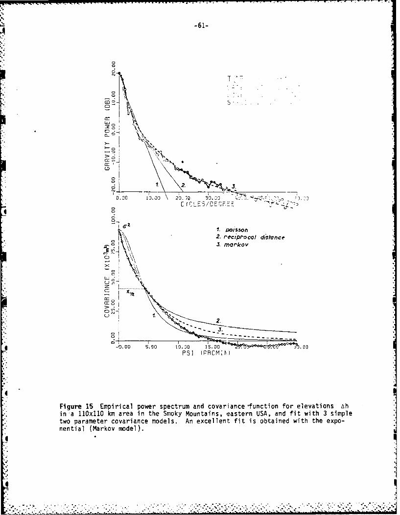
Iz -61-

0t0i

0

M

5-iXCD

C-

>5

1. 2. o .

0.0 10. 00 2 0.A 3'0. 00 - 7D.

0 C r C L E 5/D

2. reciprocal distance

C . mrkov

Di \\3

0

........... . . . . .U NJ

2.

-0.00 5.00 10.00 15.00 "-?1 1Y _ 3. .00PSI I RRCMIM

Figure 15 Empirical power spectrum and covariance-function for elevations Ahin a 110x11O km area in the Smoky Mountains, eastern USA, and fit with 3 simpletwo parameter covariance models. An excellent fit is obtained with the expo-nential (Markov model).

-.. •. ,1" -

-,'-d -": . .. . - . ''' . / . .. : ; _ . . " , " .'.:,,,- -.1: ,_...,,, . , '-"-'. ,' :" ' ' r, .'- ,l l"

.4 -62-

f (w~ =i ,f (w 2 1Tail(aw) (7.53)W

*J 1 is the Bessell function of order 1. The shape of the function fis shown

in Figure 16.

J (X)

0. 0 -0.0 2. . . 8. >)

-Figure 16

*By upward continuation to elevation H the spectrum then becomes

.6g'(u, v) = 4,ip 2L }e- H;(u, v) (7.54)

By comparison to tne "exact" terrain effect

Ai(u, v) 2TrGP e-(' A;j(u V) (7.55)

the representation error E:= Ag' -Ag is seen to be

* (u, v) =2TrGP (1 -2 iaw) ~ Ah(u, v) (7.56)

and thus

(w (2,RGo) 2 (1 -2 JI(aw) 2 e-2wH h(W) (7.57)

For deflections of the vertical essentially the same formula holds. From formula

(7.21) it is seen that the deflection error expressions corresponding to (7.56)

will be simply

S(u, v)l

n(u, V))

-63-

For an isotropic field, ¢ =nn',we get directly using the statistical indepen-

dence of and n;

Mfi() = ( ) = E{I 12 + 1 12 1 (u, V) (7.59)En E2-nE 9E

Thus, results obtained for gravity anomalies in the error analysis may be directly

applied to deflections of the vertical as well, when the previously mentioned

"conversion factor" of 6.7 mgal/arc sec is used.

To get error estirates an exponential ('Markov") model C hh(r) = G2he-r/D

will be assumed for th, topography covariance function. By (7.50) and (7.57)

the error variance wil be

C2 w o (w) dw

(2xp)2M ah w) )2 -2wH D2(2irGp )2 2 JW± (- 2 eiaw )2 e7.60Ah (1 aw [i+WD2] 3 /2 dw (7.60)

It is convenient to normalize the parameters with respect to D, introducing a

dimensionless averaging parameter a' and elevation H' = - Then by shiftD D

of variable t =wD:

G2 (21TGp) 2 (jh F2 (a', H') (7.61)E A

F2(a', H') = ; (1 - 2 Jl(a't))2 e2tH' t0 a't [l+t2] 2/ dt (7.62)

This integral has no simple analytical expression. It has been integrated numerically,

using a standard adaptive numerical integration subroutine and using polynomial ex-

pansions for J,(t) given by Abramowitz and Stegun (1965). The result (i.e. the

function F, square root of 7.62) is shown in Figure 17.

The r.m.s. computation error u at elevation H should ordinarily be

compared to the "actual" r.m.s. terrain effect a (H) at elevation H. TheC'. Ag

I'

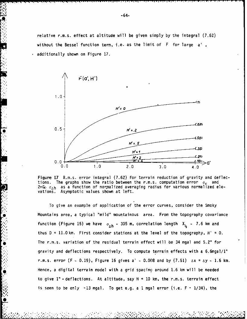
-64-

relative r.m.s. effect at altitude will be given simply by the integral (7.62)

without the Bessel function term, i.e. as the limit of F for large a',

additionally shown on Figure 17.

t:(a'. H)

1.0

H~z1)

* 0. 51H .2

so)

-.3s)H'H I

0.0 , ,> a'0.0 1.0 2.0 3.0 4.0

Figure 17 R.m.s. error integral (7.62) for terrain reduction of gravity and deflec-tions. The graphs show the ratio between the r.m.s. computation error c and2rrGp GAh as a function of nornalized averaging radius for various normalized ele-vations. Asymptotic values shown at left.

To give an example of application of the error curves, consider the Smoky

Mountains area, a typical "mild" mountainous area. From the topography covariance

function (Figure 15) we have 0 h -305 m, correlation length X - 7.6 km and

thus D = 11.0km. First consider stations at the level of the topography, H' = 0.

The r.m.s. variation of the residual terrain effect will be 34 mgal and 5.2" for

gravity and deflections respectively. To compute terrain effects with a 6.6mgal/l"

r.m.s. error (F - 0.19), Figure 16 gives a' - 0.008 and by (7.51) Ax = Ay - 1.6 km.

Hence, a digital terrain model with a grid spacingi around 1.6 km will be needed

to give 1"-deflections. At altitude, say H = 10 km, the r.m.s. terrain effect

is seen to be only -13 mgal. To get e.g. a 1 mgal error (i.e. F - 1/34), the

.i . ... .- .........- • -... ~ . ....-.. .. ."--- .'-' :. A... -.-'.-i~ .- .- - "-v ,, ".'. .. - "-"- ."-. '*

-65-

figure indicates a'- 0.7 and thus the resolution of the digital terrain model

needs to be only 13-14 km.

For geoid undulations similar error curves may be computed. In the linear

approximation height anomaly residual terrain effects at the surface of the topo-

graphy will be

2 Gp 1a (7.63)Y

Analogously to gravity and deflections the following expressions for the height

anomaly variance and error variance are obtained

2 Go 2 h+D2 f 00 dw (7.64)Y A 0 w[l+W2O2] 312

C2 (2GP)2 02 D2 f- (1 - 2 J(aw)) 1 dw (7.65)y 0 a [i+2D2]73/2

The variance a2 computed by (7.64) is infinite (opposed to the finite G2 ).E

This is a phenomena analogous to the infinite potential effect of the Bouguer

plate: very long wavelengths in the topography results in very largegeoid effects.

However, although the simple Markov covariance model used has energy at long wave-

lengths, this will not be the case for "real" residual terrain reduction with

respect to a 180x180 reference surface. Ideally, no power should remain below

-180the "reference" frequency wo0 R Thus, a better, less conservative estimate

of the "local" height anomaly variation is obtained by integrating from wo rather

than 0 in (7.64) and (7.65)

(21Gp )2 D

a2 ( 2 h 02 G2 (D, a') (7.66)

Gi (D, a') [( - 2 a dt (7.67)0

where the substitution t wD, a' = a/D, has been used again. The function

*

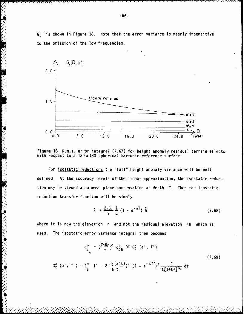
-66-

G, is shown in Figure 18. Note that the error variance is nearly insensitive

to the omission of the low frequencies.

G4 G(D, alI2.Oi -

a'= 4

a'=a

0.0 04.0 8.0 12.0 16.0 20.0 24.0 (KM,)

Figure 18 R.m.s. error integral (7.67) for height anomaly residual terrain effectswith respect to a 180 x 180 spherical harmonic reference surface.

For isostatic reductions the "full" height anomaly variance will be well

defined. At the accuracy levels of the linear approximation, the isostatic reduc-

tion may be viewed as a mass plane compensation at depth T. Then the isostatic

reduction transfer function will be simply

S27TGo 1 (1 - ewT) h (7.68)Y

where it is now the elevation h and not the residual elevation Ah which is

used. The isostatic error variance integral then becomes

2= (21r.GP2 2 D2 G (a', V)

(7.69)

G2 (a' T') = (1 - 2 Jl(a't))2 (I - tTI)2 dt0 a't t[l+t]3/

•0'.. *-' . ... . ' . .. . ' "''' .. ' . ". .- -' . . -""'2 :- 2 ' ' - : 2.2. - -- .. -''' . -- '- 2 2 -

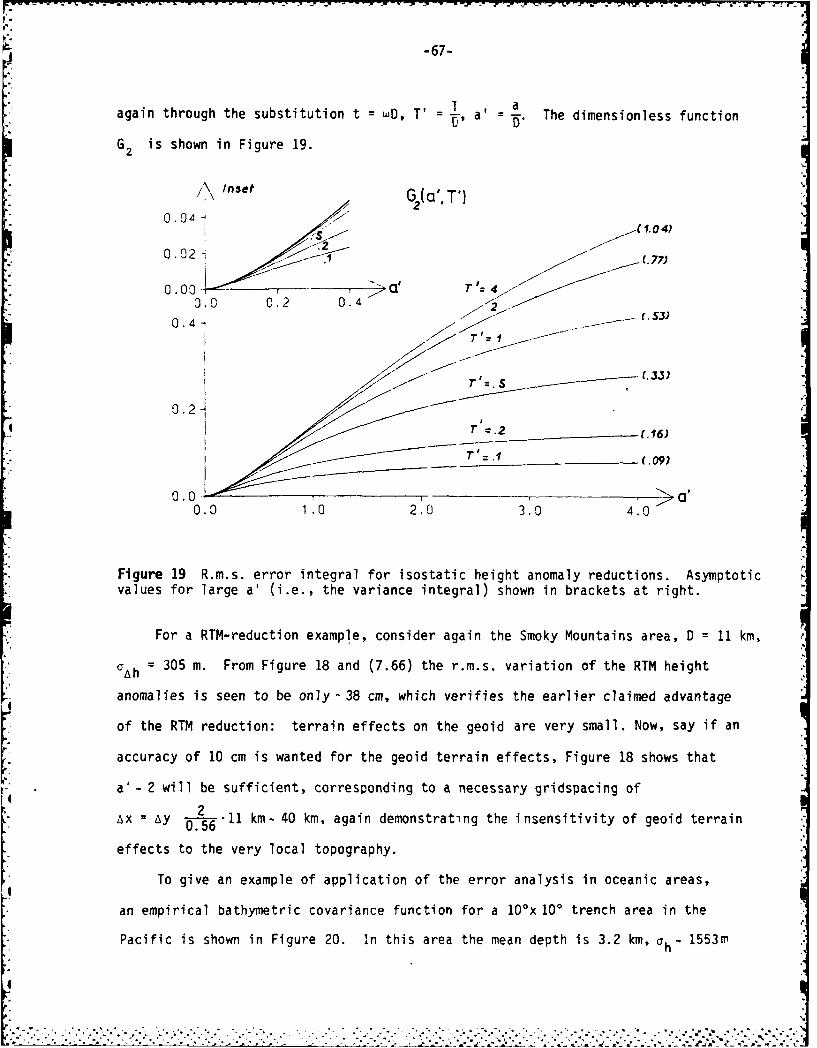
-67-

again through the substitution t = wD, T' T, a=-a'= The dimensionless function

G2 is shown in Figure 19.

insetG(',T

0.02

0.02~ (77)

00001 T•

0.0 0.2 0.4

7, 1 -

T =.2 (.16)

T '~.1(.09)

0.0 *0.0 1.0 2.0 3.0 4.0

Figure 19 R.m.s. error integral for isostatic height anomaly reductions. Asymptoticvalues for large a' (i.e., the variance integral) shown in brackets at right.

For a RTM-reduction example, consider again the Smoky Mountains area, D = 11 km,

h= 305 m. From Figure 18 and (7.66) the r.m.s. variation of the RTM height

anomalies is seen to be only-38 cm, which verifies the earlier claimed advantage

of the RTM reduction: terrain effects on the geoid are very small. Now, say if an

accuracy of 10 cm is wanted for the geoid terrain effects, Figure 18 shows that

a'- 2 will be sufficient, corresponding to a necessary gridspacing of

AxAy ---- 11 km- 40 km, again demonstrating the insensitivity of geoid terrain0.56

effects to the very local topography.

To give an example of application of the error analysis in oceanic areas,

an empirical bathymetric covariance function for a 10'x 100 trench area in the

Pacific is shown in Figure 20. In this area the mean depth is 3.2 km, 0h- 1553m

4

,,.. . " - .L' _- , ,... .. .• , ,. . . . . ..-... .. ..- -. , -. ,. .".,... ..- ".".".',"-". .. , . . .. .. "" '." " ':"

-68-

J.. C

TOPOG RPHYLRT: -20.0 - -10.0LON: 180.0 - 190.0SPRCING: 5.0' 5.0'

C -,

U-IQu j I.psoM

U_ - .. reciprocal distance

-o 3.markov;o

a.00 %0 2.00 3.00 4.00 5.00 6.00

0002. 2.0

;0--

(U

. 'Ya

02

'p3

M -

0 0

-0.00 50.00 100.00 ISO.00 200.0.00PSI (ARCMIN)

Figure 20 Power spectrum and covariance function for bathymetry in a 10Ox 100area around the Tonga trench. No reference elevations have been subtracted.Again the exponential Markov model is seen to give the best fit of the simplecovariance models. (power spectrum has been plotted for p 2.67. To get

= 1.64 results, simply subtract 2 dB from given values).

and X 107 km, giving D -155 km. For a trench area the isostatic compensation

is known to be partly based on density anomalies in the upper mantle, and therefore

a fairly deep isostatic compensation level T must be chosen. Assume e.g. T= 40 km.

Then T'- 0.26 and from Figure 19 and (7.69) with p = -1.64 the variance of the

isostatic geoid effect is seen to be a 3.4 m (a direct computation of the

. .. . .-......-. ... ......... . .;..... .. :. ;.... .. ., .. -

-69-

isostatic effects have yielded a = 3.1 m, thus validating the error analysis

approach, cf. next chapter). To compute the isostatic geoid effect with an ac-

curacy comparable to SEASAT satellite altimetry, say aE,~ 10 cm, then we must

have G2 - 0.006 and hence a'- 0.09, giving necessary grid spacing Ax- 25 km.

An "inverse" example may also be given: recently a global 5'x5' mean

bathymetry data set (SYNBAPS) was released, covering most of the earths oceans

between 750 N and 750 S. In the "rough" Tonga trench area, the SYNBAPS data cor-

responds to a'- 0.033, giving an r.m.s. isostatic computation error oE,-3 cm.

However, it should be remembered that this number corresponds to the linear ap-

proximation and mass plane condensation,and assumes the mean elevations to be

error free. Therefore SYNBAPS derived isostatic geoids might be significantly

more in error, naturally especially in areas of poor bathymetric data coverage.

8. Spectral Characteristics and Covariance Functions for Local Topography and

Terrain Effects

In the present section key parameters describing the statistical behavior

of the local topography will be investigated for a number of different sample

areas, representing various types of topography, from nearly flat to alpine areas

in the United States.

Power spectrum and covariance functions have been estimated from available

0.5'x0.5' elevations, supplied by the National Geodetic Survey, using a simple

FFT approach.

With this approach, the residual topography power spectrum (power spectral

density) is obtained from the discrete fourier transform (7.37) of Ah by

h h(U, v) = nm I(u, v)12 (8.)Ah ' Ax~y

where Ax, Ay are grid spacing of the nxm given elevation grid. The power

spectrum t, will be defined in a frequency square between the Nyquist fre-

1

..4 .. .., .' ..= ",- ..... .: ,b ,.,i,. "," " ,:. , ', " . : ", -:. ., ." '' ' -'" :

-70-

quencies (7.40) ±uN, ±vN. It will be symmetric with respect to the zero-frequency:

O(u, v) = 0(-u, -v). By the inverse fourier transform (7.38) the 2-dimensional

covariance function is obtained:

i C~hh(X, ) = xAy -1CAh (x, y nm OAhAh(u, v) (8.2)

This function will be defined within the square +.x, Ay, and will again exhibit-2 -2

symmetry with respect to (0,0).

In the sequel 0 and C will be investigated in a number of cases for both

topography, terrain corrections and observed gravity and geoid. Since we are

mainly concerned with isotropic processes, the results will be averaged along

circles, to give the "isotropic" covariance function C(r) and power spectrum

. However, to get an idea of the anisotropy, a contour plot of the 2-dimen-

sional covariance function will be given as well. For gravity also degree-vari-

ances will be given, based on formula (7.54).

The power estimate (8.1) may be improved by taking the finite extent of the

given data into account through the use of window filters. For tests, a two-

dimensional Hanning window has been applied in the frequency domain (see e.g.

Engelis, 1983), the main effect being a less "noisy" O(u, v). The discrete Hanning

window in the frequency domain is nothing but a simple smoothing, with a filtered

frequency value given as a weighted mean of the value itself and the adjacent

frequencies. Since this smoothing already to some degree is performed by the

radial smoothing (and the prime interest is in the overall shape of the curves)

I have found no practical need for windowing, and thus the spectral estimates

represent "raw", unfiltered FFT-results.

Examples of results have already been shown in Figures 15 and 20. The power

spectra will be given in units of mgal 2degree 2 (1 degree- 111 km), where elevations

have been converted to gravity using the simple Bouguer factor for p = 2.67 g/cm 3.

-- Z6""

. . . . . . . .."*;'.; -', K".- ;' >"..'; ?- . . "- ''. , .. '.- "---' " i..,.,;/'. - - '.'.''•;'. -.. . ..... . . ......-.. . .-.. . .,.-.... ..- • -- , *.-

-71-

= 2Gpah - 0.1119 [mgal/m] Ah (8.2)

and results are shown logarithmic in dB

P [dB] = 10 log1 0 (o [mgal2degree 2]) (8.3)

as a function of the frequency v in units cycles/degree.

The anisotropy will be indicated through a small contour plot of the normalized

2-dimensional covariance function at levels C(r) = 1.0, 0.8, 0.6, ... (Figute 21).

To get a quantative measure of the anisotropy, an anisotropy index will be defined as

anisotropy index = maximal X (8.4)=minimal X .4

where X- is the correlation length in a certain direction, i.e. the distance

from origo for which the covariance is half its zero-value CO. An isotropic0

field will have an anisotropy index of 1.

The second-order gradient variance G will be used in the sequel as a measure0

of high-frequency content. As shown by Moritz (1980), Ga will be given as the

curvature of the (gravity) covariance function at origo. It will be estimated

directly from the empirical covariance function, using a symmetrical spline inter-

polation procedure. The result must be used with some caution, especially for

the topography where the applied Bouguer-approximation is very crude for second-order

gradients. Since the spline curvature determination will be directly dependent

on the data grid spacing, Go will merely represent a lower limit of the gradient

variance, giving the gradient variance of some smooth, filtered version of the

actual gradient field. The gradient variances will be given in E2 ,

1E 10- 9s 2 = 0.1 mgal/km.

4..............................

• .- .'. -?' ./ ?' T .:. ' . .. -..-. ° . -. " -- ', . ..-"? -- :, ? ? .- I '. .'.Z.*- ,., o ,

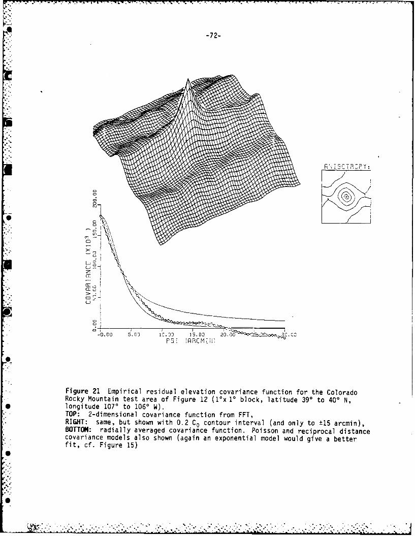
-72-

CD

CD

L.n

0 -

-0.00 5.00 10.00 15.00 20. '0PSi IRAPCM IJ)

Figure 21 Empirical residual elevation covariance function for the ColoradoRocky Mountain test area of Figure 12 (l0x 10 block, latitude 390 to 400 N,

* longitude 1070 to 1060 W).TOP: 2-dimensional covariance function from FFT,RIGHT: same, but shown with 0.2 CO contour interval (and only to ±15 arcmin),BOTTOM: radially averaged covariance function. Poisson and reciprocal distancecovariance models also shown (again an exponential model would give a betterfit, cf. Figure 15)

" "" .•• , "" - . - - " .- .TT- , . ;: ... . . . . . . .

-73-

8.1 Topographic Covariance Functions for U.S. Sample Areas

A number of l0x 1.20 nearly square blocks (each containing 120x144 elevation

points) have been analyzed using 0.5'xO.5' (-1 km) elevations from the NGS data

base. Each analysis, with FFT, plotting etc., used c.5 sec CPU-time on The Ohio

State University's Amdahl computer.

The areas are shown in Figure 22, and represent various types of topography:

alpine (Colorado, Sierra Nevada), alpine-mountainous with volcanoes (Washington),

mountainous plains (New Mexico), older mountains (Smoky Mountains) and flat to

hilly lowland (Ohio). The two 10 New Mexico blocks comprise most of the "White

Sands" New Mexico test area for comparison of gravity field modelling techniques,

see e.g. (Tscherning and Forsberg, 1983).

All elevations analyzed are residual elevations Ah = h - h ref , where the

180x180 spherical harmonic expansion of the earth's topography of Rapp (1982)

has been used as reference elevation. The Bouguer-derived topographic gravity

is thus to first order the RTM180 terrain effect.

Results are shown in Figures 23, 24, and Table 4. Despite the different

types of topography, the results are amazingly similar, with the prime variation

being in the r.m.s. variation of C0 , less in the shape of the curves and the

correlation length. The correlation length varies in the range 6.5-12.2 km, while

the r.m.s. residual elevations varies from 45 m to 785 m. For the eight test

areas, maximal and minimal roughness of RTM-terrain effect field is obtained in

the Sierra Nevada and Ohio blocks respectively: for gravity the r.m.s. terrain

effect will be 88 and 5 mgal respectively, for deflections 13" and .8" and for

height anomalies 96 cm and 5 cm, using the results of section 7.8. The degree

of anisotropy is seen in some cases to be nil, in other cases rather severe.

Since the observed gravity field will be dominated by the topographic effects

in mountainous blocks, the same degree of anisotropy will be expected in the

gravity covariance function, thus stressing the need for utilization of terrain

reduction methods.

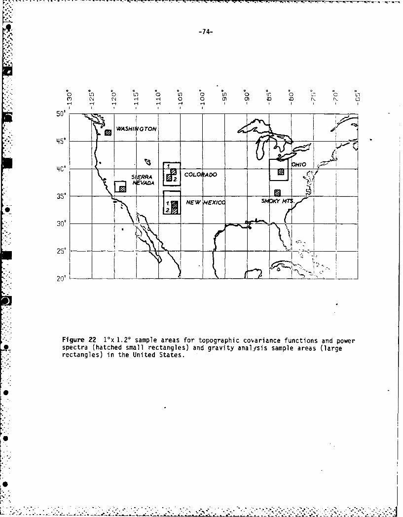
0 In 0 a a 0 an 0 an 0 oN 0 0 CM Co Co NI N 1 Lj

WASHI G TON

450

4Q~r ___ * HIO 2 _ _

350 SAERRA COLORADO

1. NEW MEXICO SX Mr.

30' %_j0125' _

Figure 22 10x 1.20 sample areas for topographic covariance functions and power* spectra (hatched small rectangles) and gravity analy~sis sample areas (large

rectangles) in the United States.

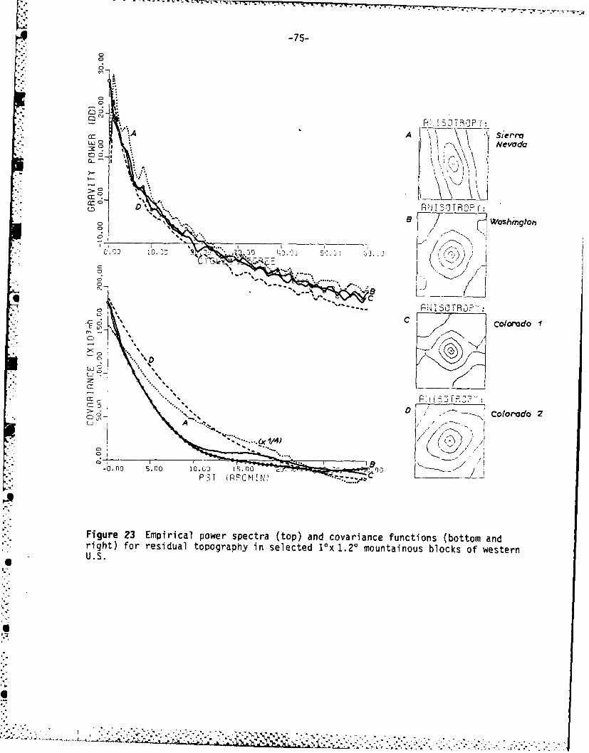
LI5CD

0

AA sierreLU0 D Nevada

V1 C;-:C L .j

E2

Was hmn gom

0. r 10.20 s,' DO j-. GO3 002

C ~C

C, CCoo'd

D Colorado 2CD.

-0.00 5.00 10.0') -10

Figure 23 Empirical power spectra (top) and covariance functions (bottom andright) for residual topography in selected 1"x 1.20 mountainous blocks of western

U.S

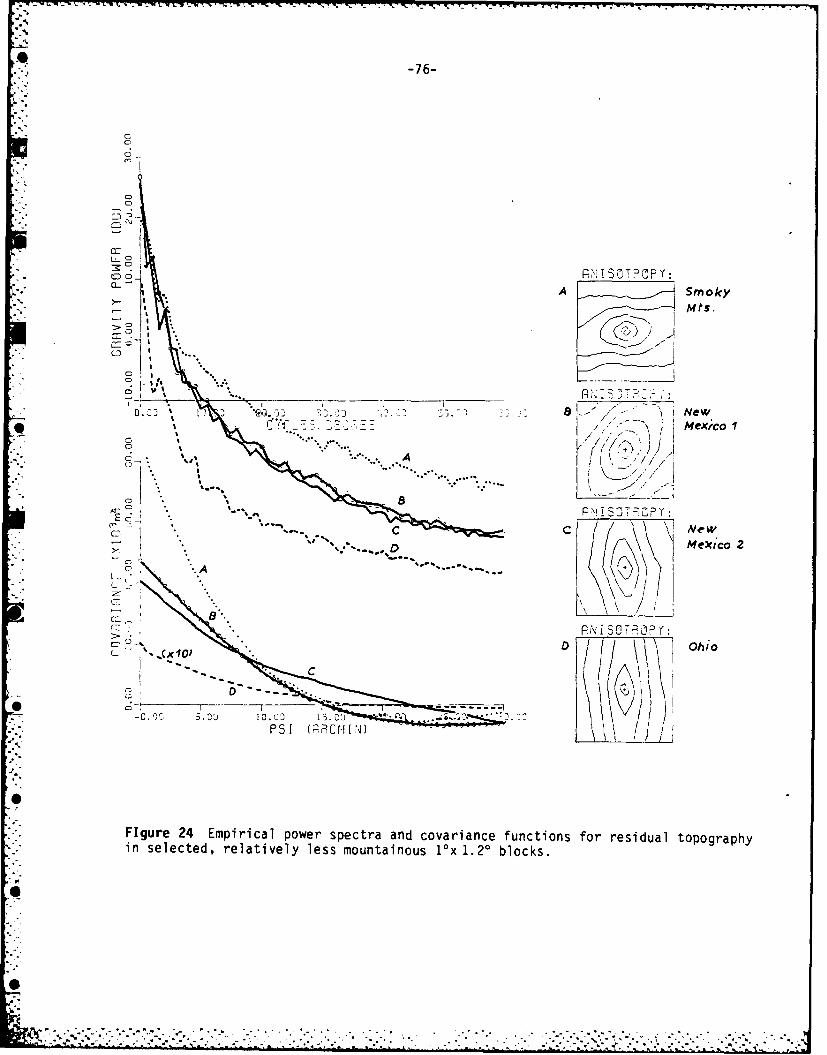
-76-

C:

CD

C

RN I SOT? OP Y:C -A Smoky

C

... .. D0....................................

* .. ----A

.A **C C Ne

'(X 10j Ohio

C(D C

PSI (PFCm[Nj L

FIgure 24 Empirical power spectra and covariance functions for residual topographyin selected, relatively less mountainous 10x 1.20 blocks.

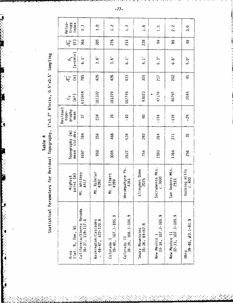
-77-

u,) -) r-. C)0 C\j 0~ 4

C'

u. 1.0 i

ca - i- n LO I

Ln o j r- Cj

00 oC 0 CSJ m- 0CD - CD.-:r cn 8\I in'Nr.

C\J~ fn ~0 0 0

C3

inj ca. r- K % CI:> ' ca . 0) m. rn toC~

a) -I-. o: 1 -

I In

CLI ~0)I IA

r0 m C j 1f

4.) -L E

a. c C

4.- c4:fciI

.n CI LO

M1 m) 0 o 0 -0

:a CL E- u0 E 0c

-Ca' 41F- 00 00 01u- ~I ~~~~L m cu. v ~ - C~ ~ >

0 '3 CI Ci cII I

2: co (AC3n n

V)~~~ . . C* -a V) L C~i D - C) - CD

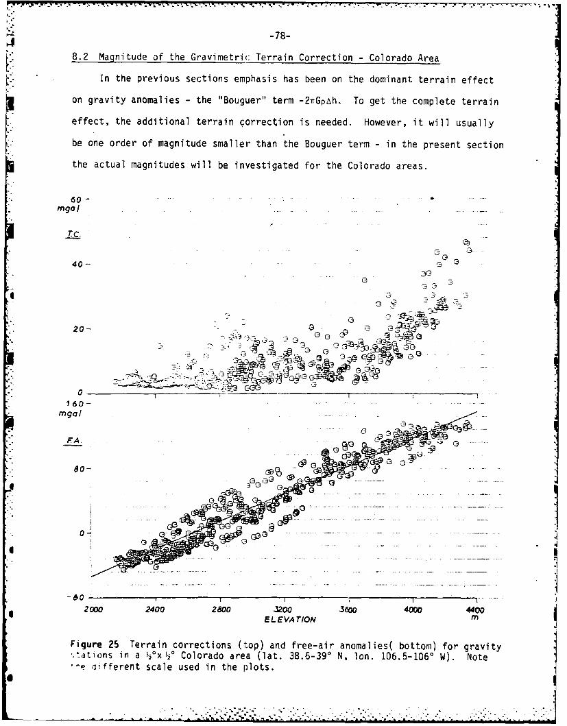
-78-

8.2 Magnitude of the Gravimetric Terrain Correction - Colorado Area

- In the previous sections emphasis has been on the dominant terrain effect

on gravity anomalies - the "Bouguer" term -27rGpAh. To get the complete terrain

effect, the additional terrain correction is needed. However, it will usually

be one order of magnitude smaller than the Bouguer term - in the present section

the actual magnitudes will be investigated for the Colorado areas.

60 -

i. C___ ,

40- . 33(

40 ...... 3 -3 ..

20- G3

D 3 P

C-4)

* 0 -160-

remgal

PA.

60- (

.. . .. .. ...'..

. ......... . .. 42000 2400 2800 3200 3S0 4000 4400

E LEVA TION l

Figure 25 Terrain corrections (top) and free-air anomalies( bottom) for gravity',.ations in a 0°x ° Colorado area (lat. 38.6-390 N, Ion. 106.5-1060 W). Note-e ilfferent scale used in the plots.

i-

- - 7 1 Y _W 7'1." -.7 -7 -7 W 7

-79-

Figure 25 shows an example of actual gravity data and terrain corrections

for a small ( 0x 0 ) block (NGS data). The trrain corrections are seen to be

in the range of 0-40 mgal, opposed to a Bouguer RTM-effect range of roughly -120

to 120 mgal. For such a rather small area, the free-air anomalies correlate well

with elevation, the slope being essentially a measure of the topographic density.

However, since the terrain corrections have a tendency to be large for the higher

stations, the free-air slope will give too low density values: in the case of

Figure 25 p- 2.1, which is unrealistic. Therefore, while terrain corrections

might be neglected in connection with e.g. error studies, omission in other cases

implies serious systematic errors, especially when used for density determination

as outlined in Section 5.

To study further the terrain correction, computation of terrain corrections

was done in a 2'x3' grid for the two lx10 Colorado blocks of the last section

(and on a 2'x2' grid for the x 2 area of Figure 25), using the prism integration

programme of the appendix. The choice of the rather coarse computation grid size

was necessary to avoid excessive computation times (on the OSU Amdahl system

CPU-time requirements were c. 0.2 sec/station). Figure 26 shows the result for

the northeastern block. By comparing to the topographic map (Figure 12) it is

clear that some degree of undersampling is done by only computing on a 2'x3' grid,

so some aliasing might be expected in the power spectra of the terrain correction

signals, shown in Figure 27.

At the 2' resolution level, the terrain correction covariance functions (Figure

27) might be described as a "white noise" signal with very short correlation length

plus a smaller long wavelength signal (remote zone effects). Compared to the

main "Bouguer" terrain effect, the terrain corrections are indeed seen to be smaller,

as shown in Table 5 - however, large outliers and non-normal error distribution

makes it important to use the best possible terrain corrections for gravity field

modelling, using even more detailed elevation data than the presently used 0.5'x0.5'

heights.

. .....-. .. . ".- . . . . .. . .-.. . . .- . . .- ". . ."i i-.-i"- , """ ' " " "" . ' ' , -' * .-

*: "

.' "" - ' "' - "- . .

-80-LONGITUDE

253 254

00

I-

0 E0

0/

39 - +-~N39253 254

Figure 26 Terrain corrections in mgal for "Colorado V" 1*x 10 block, computedon a 2'x 3' grid. A topographic map of the same area is shown in Figure 12.

-81-

0

2El___________________________________RNI SOTROPY: ae* area 2

0.00 2.50 5.00 7.50 10.00 12.50 15 .00CYCLES/OEGREE

0~

0

in RNISOTROPY:area

ccI

~~2

- 0.0 S0 00 1 .0 2 .000S RRMN

Fiue20oe pcr n oainefnto o h rvmti eri

corcini w xV bocso ooao h anteri fetadtoal

shwqihdtc.Fgr 3

-82-

RTM Bouguer term

(mgal) Terrain corrections (mgal)

Area r.m.s. X mean std. dev. max X

I (39-400 N, 107-106 ° N) 47.7 3.5' 6.4 4.4 55 1.8'

II (38-390 N, 108-1070 N) 48.5 6.1' 4.8 3.7 29 2.4'

III (38.5-390 N, 106.5-106- W) 51.9 4.6' 6.4 4.4 27 2.4'

Table 5 Gravity terrain corrections, Colorado areas.

The obtained mean terrain corrections may be used to test S~nkel's approx-

imate formula (cf. Section 7.2):

mean terrain correction - 3irGp k (8.5)

For the three areas, values of 4.7 mgal, 2.8 mgal and 4.2 mgal are obtained.

*-- The mean terrain corrections obtained by (8.5) are thus seen to be somewhat too

low (this deficiency is primarily a consequence of the tendency of the topographic

covariance functions to be exponential: for such covariance function the integral

formula underlying (8.5) is undefined, cf. Sunkel, 1981a, p. 62).

- . 8.3 RTM Geoid Effects - Colorado Area

When using a residual terrain reduction with respect to a180x180 spherical

harmonic elevation reference surface, the study of section 7.8 showed the terrain

geoid effects to be fairly small. In this section, an example of actual magnitudes

encountered in an extreme case - the mountainous part of Colorado - will be given.

The 40x40 block of Figure 22 - comprising essentially all of Colorado west of0

Denver - will be studied based on 4'x5' mean elevations.

Figure 28 shows the residual topography covariance function for the 4'x 5'

elevations. RTM geoid undulations were computed from this grid in a "fixed-area"

reduction taking only into account the 4°x4* square. The geoid effects varied

from 1 to -3 m with a mean of -80 cm and an r.m.s. variation of 87 cm with respect

'. - ' ... . . . - ".'.'- - . . • -. - ... * ... • " """"" "" .. ' .-L. L .. ''- .- " ..-. '--. , - " " "

-83-

-. ,z.

cc

cc

C

C'

0.00 20.00 U0.00 60.00 1 0 120.00PSI (RRCM[N)

9RNISOTPT:

0

o

9

C,,-

"°U

Cr

Cr0

4 LU

C)

DU"

0.00 20. 00 -. 9A 0_ F0. 00 80. 00 100. 00 120,.00

Figurie 28 Covariance functions for residual topography (lower) and computed RTM-180geoid effects (upper) for the mountainous part of Colorado. The 180x180 referenceelevation surface is seen to give a good fit in Colorado, the height covariancesbeing near zero for , > I1.

to the mean (Figure 29), corresponding to indirect effects on gravity anomalies

below 1 mgal. For comparison, using the statistical study of Section 7.8, the ele-

" vation covariance parameters (a Ah = 369 m, X = 8.4') yields an r.m.s. geoid

variation of 66 cm, the slightly too low value being primarily due to the remaining

small long-wavelength geoid effects, evident from Figure 28.

10-,

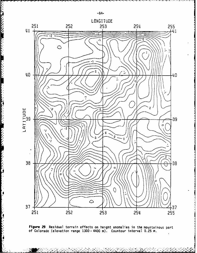
I - ., 6.- m

-84-

LONGI TUDE251 252 253 254 255

41 -1-2 ---

04

00

I--

404

25

- Figure 29 Residual terrain effects on height anomalies in the mountainous part* of Colorado (elevation range 1300 -4400 in). Countour interval 0.25 in.

-85-

9. Terrain Reductions: Spectral Characteristics and Covariance Functions forLocal Gravity

By using known density anomalies in gravity field modelling, the purpose

is to obtain a more smooth field, more suitable for interpolation and prediction.

In this section the actual smoothing obtained using the residual terrain reduction

will be studied for a number of U.S. sample areas, shown in Figure 22, each repre-

senting various types of topography and geologic setting: the 2'x 2° Sierra Nevada

block contains the highest part of the Sierra Nevada mountains plus a part of

the California Valley, and is characterized by a large horizontal gravity gradient,

relating to changes in crustal and upper mantle structures. The 4°x4 0 Colorado

block has high mountains all through, anda thick crust giving rise to very low Bouguer

anomalies. The 40x4* N ew Mexico block has both mountains and plateau-type topo-

graphy, and major density anomalies associated with the Rio Grande rift system.

Finally, the 40x40 Ohio area represents lowlands and an area geology of primarily

thick paleozoic sediments.

The 4 areas have a reasonable coverage of terrestrial gravity anomalies in

the NGS data base. To obtain covariance functions and power spectra of the data,

the terrain-corrected Bouguer anomalies were gridded in a 4'x5' (ca. 7.5x7.5 km)

grid, using a truncated collocation gridding algorithm (Cruz, 1983) where the

value at a point is obtained from the 5 closest neighboring points (used subsequent

to an initial thin-out screening, where only one data point per 1'x1' "pixel"

was retained). An example of the obtained Bouguer anomaly grid is shown in Figure 30.

To obtain RTM-gravity anomalies, relating to a 180x180 spherical harmonic

expansion, use is made of (7.5):

RTM anomaly Agc = Ag - 2G, (h - h ref+ tc (9.1)

For local gravity field modelling, a 180x180 spherical harmonic gravity reference

field corresponds as earlier mentioned to the RTM reduction. Thus, by (9.1) the

terrain-reduced gravity anomalies, referred to a 180x180 reference gravity field,

..v

. -"'" I! ; '"" " """" ". ""- . -". - . " -.- '" .' " -" -".' .' -" " - ' ."•"- ' ". - ' ."' "'

-86-

LONGI TUDE251 252 253 254 255

SS

02

404

* 251252 53 24e25

Figu~re 0Buuraoaisi h ooaobok hw ih5ma otusGrait stto lctos hw it os

0C

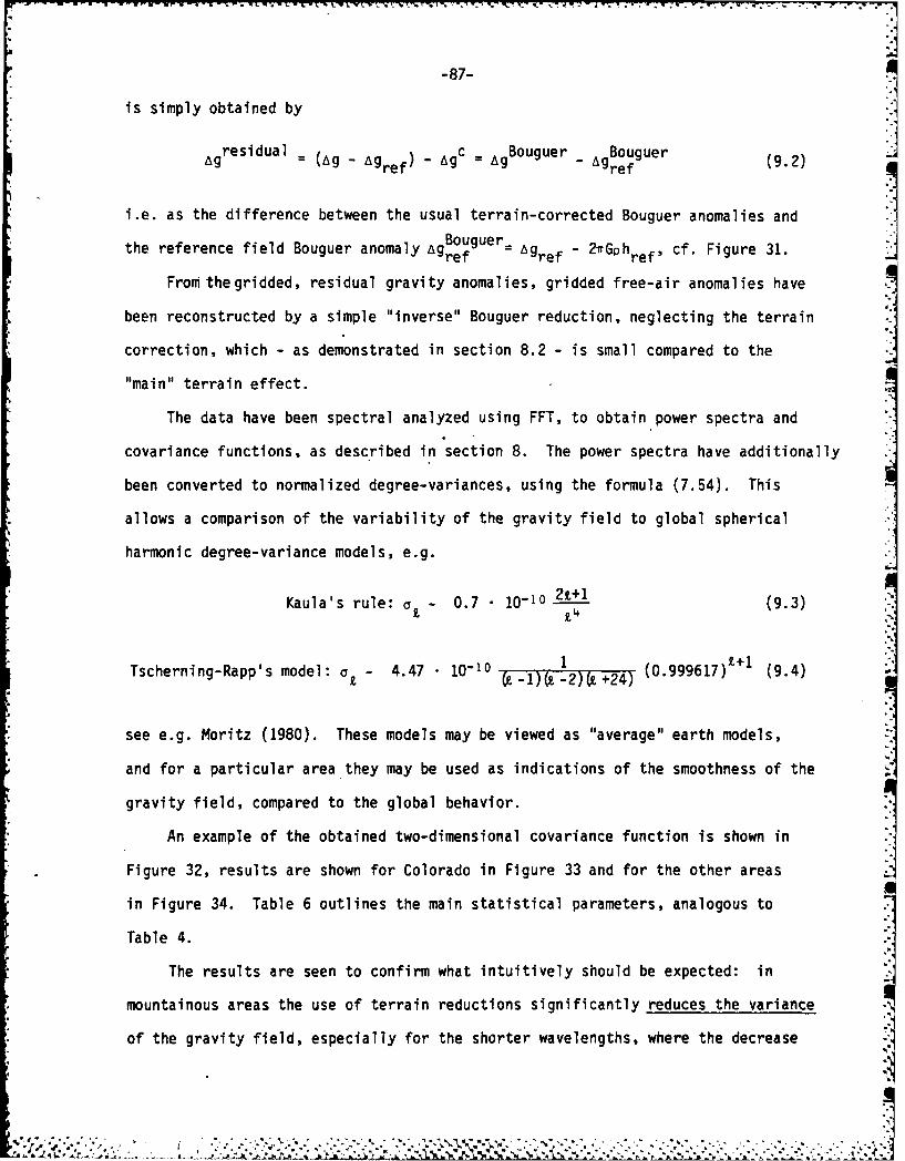
-87-

is simply obtained by

,gresidual = AAgc = uguer AgBouguer (9.2)red gc Ag rfef

i.e. as the difference between the usual terrain-corrected Bouguer anomalies and

ougeugnomlyr_~ - 2 G cf. Figure 31.the reference field Bouguer anomaly Ag ref - Aref - h ref , f igr 1

From thegridded, residual gravity anomalies, gridded free-air anomalies have

been reconstructed by a simple "inverse" Bouguer reduction, neglecting the terrain

correction, which - as demonstrated in section 8.2 - is small compared to the

'main" terrain effect.

The data have been spectral analyzed using FFT, to obtain power spectra and

covariance functions, as described in section 8. The power spectra have additionally

been converted to normalized degree-variances, using the formula (7.54). This

allows a comparison of the variability of the gravity field to global spherical

harmonic degree-variance models, e.g.

Kaula's rule: - 0.7 10-10 21+1 (93)

Tscherning-Rapp's model: a 4.47 10-10 1I-2) +24) (0.999617)'+ (9.4)

see e.g. Moritz (1980). These models may be viewed as "average" earth models,

and for a particular area they may be used as indications of the smoothness of the

gravity field, compared to the global behavior.

An example of the obtained two-dimensional covariance function is shown in

Figure 32, results are shown for Colorado in Figure 33 and for the other areas

in Figure 34. Table 6 outlines the main statistical parameters, analogous to

Table 4.

The results are seen to confirm what intuitively should be expected: in

mountainous areas the use of terrain reductions significantly reduces the variance

of the gravity field, especially for the shorter wavelengths, where the decrease

* .

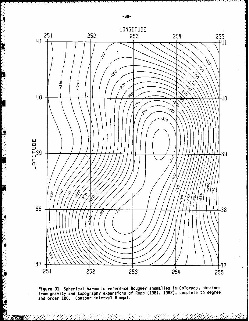
-88-

LONG ITUDE251 252 253 254 255

0 o

'100

U]

1*-9

-j

253 25V 25

Fiur 31Shrclhroi eeec oge nmlenClrdotInefrom grvt n oorpyepnin fRap(91 92,cmlt odgean rde 8.Cnoritra gl

383

37 7

2S 25 25 2S 255

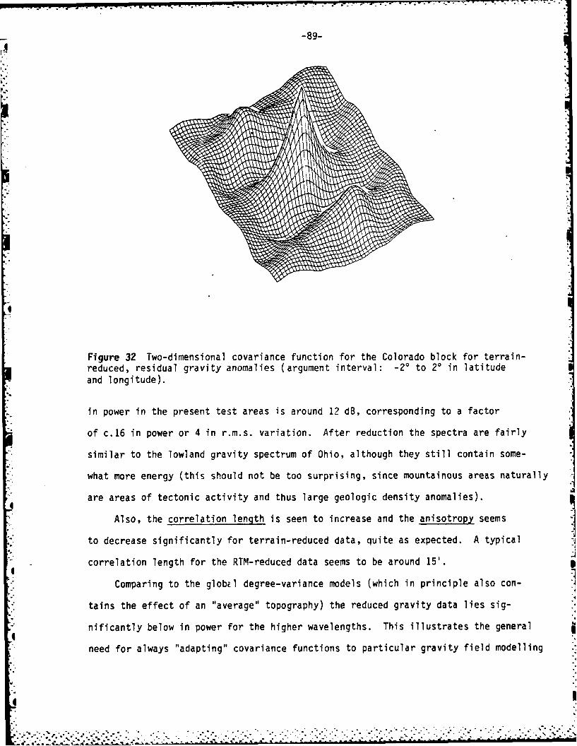
-89-

Figure 32 Two-dimensional covariance function for the Colorado block for terrain-reduced, residual gravity anomalies (argument interval: -2' to 20 in latitudeand longitude).

in power in the present test areas is around 12 dB, corresponding to a factor

of c.16 in power or 4 in r.m.s. variation. After reduction the spectra are fairly

similar to the lowland gravity spectrum of Ohio, although they still contain some-

what more energy (this should not be too surprising, since mountainous areas naturally

are areas of tectonic activity and thus large geologic density anomalies).

Also, the correlation length is seen to increase and the anisotropy seems

to decrease significantly for terrain-reduced data, quite as expected. A typical

correlation length for the RTM-reduced data seems to be around 15'.

Comparing to the global degree-variance models (which in principle also con-

tains the effect of an "average" topography) the reduced gravity data lies sig-

nificantly below in power for the higher wavelengths. This illustrates the general

need for always "adapting" covariance functions to particular gravity field modelling

4c

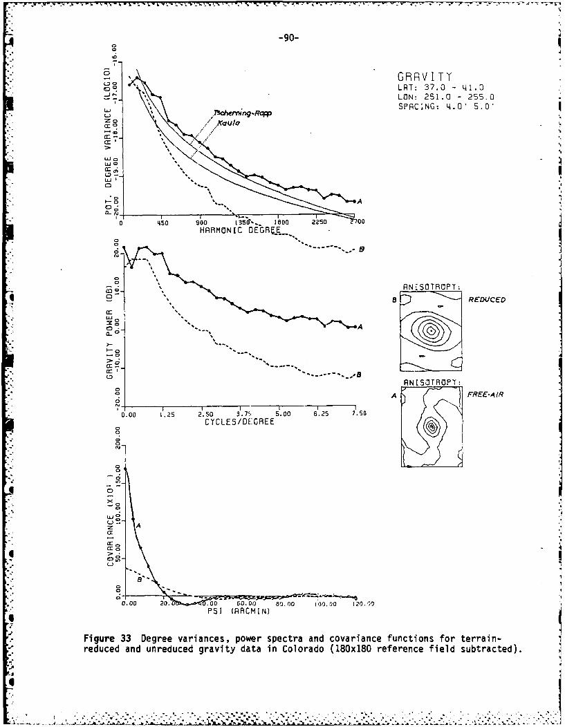
-~~V W. ~ - '

-90-

LRT 370 -41.0

I~cheningRqcpSPROING: 4.0' 5.0'Z 0 Kaula

c

o A

e. j

0 4150 900 13561... 1600 2250 00HRAM'ONIC OEGR KE_

E.=;_ %,ANISOTROPY:C %,8 DREDUCED

cc: 1Ii

Cr E 0r R

0

0.0 1.2 0 3.7, 5.0 62 5

UJ0

C

0r

0 .00 20. 80.00 100.00 120. r0

PSI (RRCMIN)

Figure 33 Degree variances, power spectra and covariance functions for terrain-reduced and unreduced gravity data in Colorado (180x180 reference field subtracted).

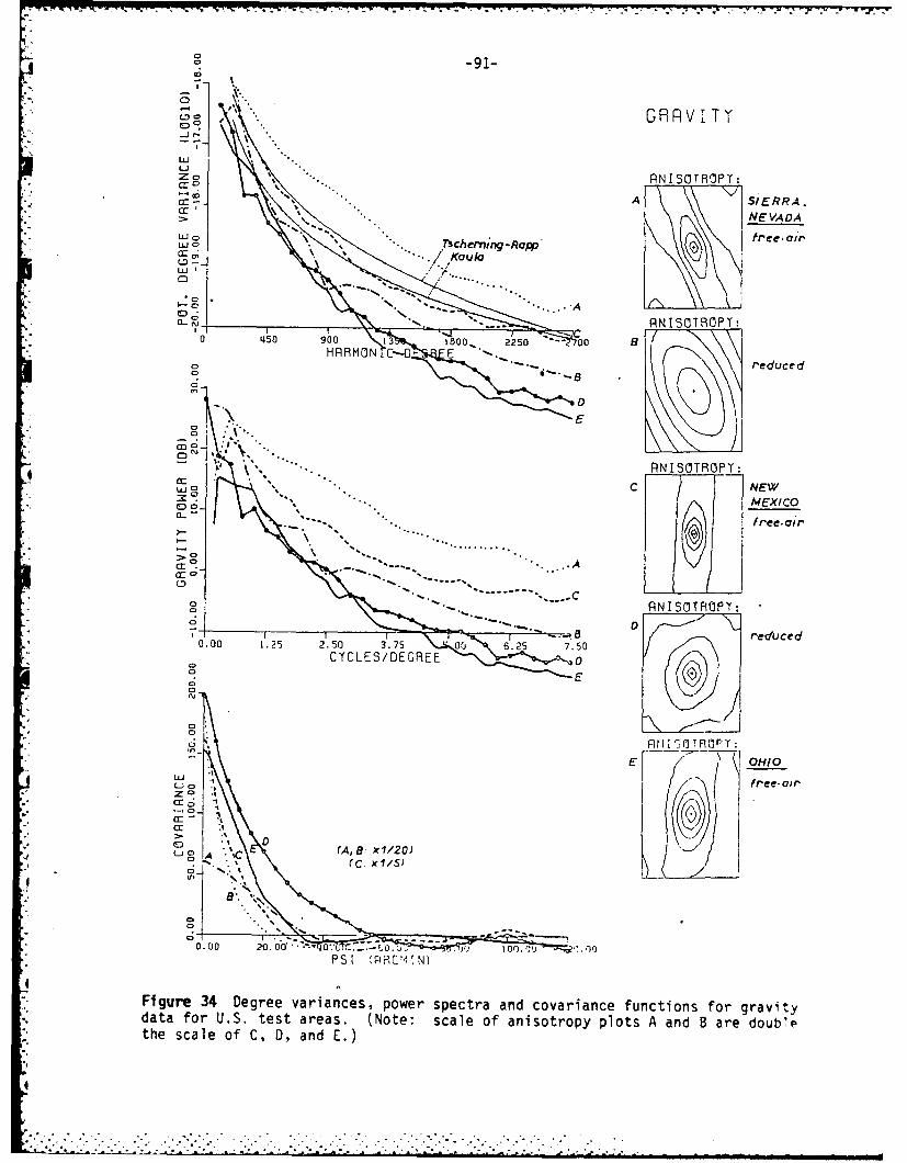
9 -91-

GRA V TI

LU

ZoCr ANISOTROPY:

* .-. A SiERRA."~ . NEVADA

U 0 free-ai-". \ .* Tscheming -Rapp'

LU'

0 .. A0 *

- sCL N*5 A-NISOTROPY:

0Lisa 900 13 1800- 2250 -~ 00

oHRRMON C-0 E reduced

D

E

ANISOTR~OPY:

CDC

a.. - reduced

_71

cr:

0.00 20.5 2a .5 .. . 75 Oi 60.5 7.0.

Figre34DegeevaiacYes oer ectan coaiac fntofogrvtdaafrUS0etaes Nt:saeo nstoyposAad8aedu~

th 0cl fCD n .

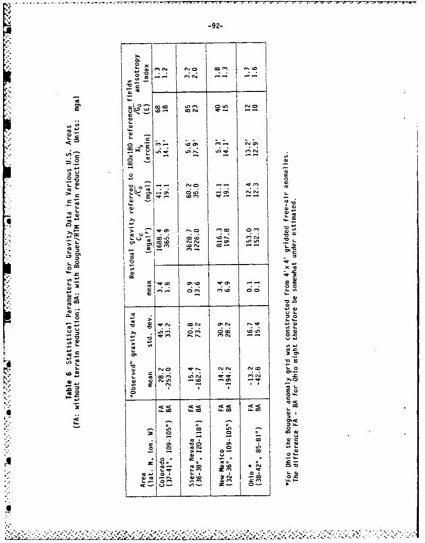
-92-

OS-xW M C. i00

u - - c CS - 4-

4An

-V x10 CD)4~O ~ ~ 0

0 W

00

C~p

1- c

S- c- -U

IVVS- CC' - 00 L 0% LC

SE C

0 0

a , ' * - w

-cr C4 co i m f, -c 4

.61

V)U,+

to S

"1o 0 0 %41-

6LL C Ij.. M -an LL co

0o co 0

CD I =U Ij

0 0j C Lo 4- L

W U 04-

* 0 0 .,0m I"O CO 0~

'a1- 0 1 Li I CI LW aW'Ut -CD %0' C~j CO- 0..=

______________M_ _____________ en _____________ P__________

64

-~ ~ -!- AZ**** r*..-

-93-

area: the global covariance models must generally be modified to have less power

at higher frequencies. For the free-air gravity data, only the New Mexico block

is seen to be of fairly typical "global" type. This block is thus a good repre-

sentative test area for gravity field modelling experiments.

The general conclusions of this section supports the results of the extensive

study of North American gravity covariance functions by Lachapelle, Mainville

and Schwarz (1983). That study, based on 5'x5' gravity data and using a completely

different approach than here, shows parameters in good agreement with relevant

parts of Table 6., e.g. for "block 11" of that study, covering most of Colorado, a

free-air Co-value of 2071mgal 2 is given, opposed to the 2061 mgal 2 obtained here.

For the gravity gradient variance Go, the average for "block 11" is c. 1750 E2

compared to 4620 E2 of Table 6 for unreduced data, and c. 400 E2 versus 324 E2

for "terrain-reduced" data.

These G0-values are probably much too low, the spacing of the data being

simply too large. An example: for the 2°x 2° Colorado area 38-40 ° N, 107-105* N

(which has a dense gravity coverage), a computation of G based on 2'x 2.5' data

have yielded G0-values of 1410P and 1006 E2 for unreduced and reduced data respec-

tively - and by utilizing the topography results of Table 4, a 0.5'xO.5' data

grid would be predicted to yield G 0-values around 60000 E2 for free-air anomalies!

This shows, that the G0-quantity is nearly meaningless in mountainous areas -

only combined with a suitable filtering through well-defined mean value operators

or upward continuation do the second-order gradients have well-behaved statistical

parameters.

.. •. -,. .'.- . . , .,. , . . ,.,.,'.. . .".. .... . . . . .,.. . ... - - .". ,- . . - - . . , . ' ,. ,' . . .

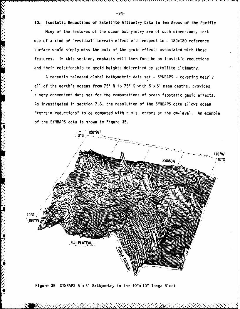
-94-

"- 10. Isostatic Reductions of Satellite Altimetry Data in Two Areas of the Pacific%"

Many of the features of the ocean bathymetry are of such dimensions, that

use of a kind of "residual" terrain effect with respect to a 180x180 reference

surface woufd simply miss the bulk of the geoid effects associated with these

features. In this section, emphasis will therefore be on isostatic reductions

and their relationship to geoid heights determined by satellite altimetry.

A recently released global bathymetric data set - SYNBAPS - covering nearly

all of the earth's oceans from 750 N to 75' S with 5'x5' mean depths, provides

a very convenient data set for the computations of ocean isostatic geoid effects.

As investigated in section 7.8, the resolution of the SYNBAPS data allows ocean

"terrain reductions" to be computed with r.m.s. errors at the cm-level. An example

of the SYNBAPS data is shown in Figure 35.

-- - l3"w.100. ..--

Si.*

Figure 35 SYNBAPS 5'x 5' Bathymetry in the 10*x 100 Tonga Block

6%

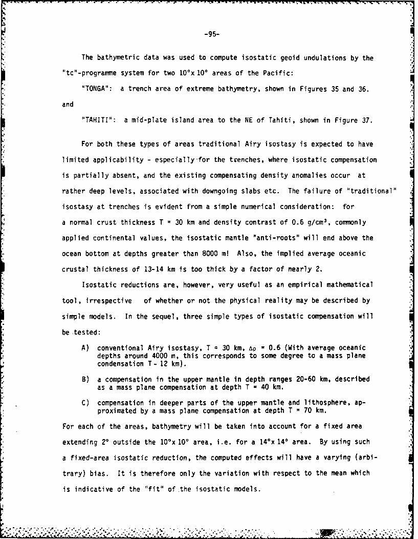
-95-

The bathymetric data was used to compute isostatic geoid undulations by the

"tc"-programme system for two 10Ox 100 areas of the Pacific:

"TONGA": a trench area of extreme bathymetry, shown in Figures 35 and 36.

and

"TAHITI": a mid-plate island area to the NE of Tahiti, shown in Figure 37.

For both these types of areas traditional Airy isostasy is expected to have

limited applicability - especially-for the trenches, where isostatic compensation

is partially absent, and the existing compensating density anomalies occur at

rather deep levels, associated with downgoing slabs etc. The failure of "traditional"

isostasy at trenches is evident from a simple numerical consideration: for

a normal crust thickness T = 30 km and density contrast of 0.6 g/cm 3 , commonly

applied continental values, the isostatic mantle "anti-roots" will end above the

ocean bottom at depths greater than 8000 m! Also, the implied average oceanic

crustal thickness of 13-14 km is too thick by a factor of nearly 2.

Isostatic reductions are, however, very useful as an empirical mathematical

tool, irrespective of whether or not the physical reality may be described by

simple models. In the sequel, three simple types of isostatic compensation will

be .tested:

A) conventional Airy isostasy, T = 30 km, ap = 0.6 (With average oceanic

depths around 4000 m, this corresponds to some degree to a mass planecondensation T- 12 km).

B) a compensation in the upper mantle in depth ranges 20-60 km, describedas a mass plane compensation at depth T = 40 km.

C) compensation in deeper parts of the upper mantle and lithosphere, ap-proximated by a mass plane compensation at depth T = 70 km.

For each of the areas, bathymetry will be taken into account for a fixed area

extending 20 outside the 10°x 100 area, i.e. for a 14°x 140 area. By using such

a fixed-area isostatic reduction, the computed effects will have a varying (arbi-

trary) bias. It is therefore only the variation with respect to the mean which

is indicative of the "fit" of the isostatic models.

". '. - ,"d " ". " "" -"." " "" "" -'"* - . . .". *- ,'-. . '-"

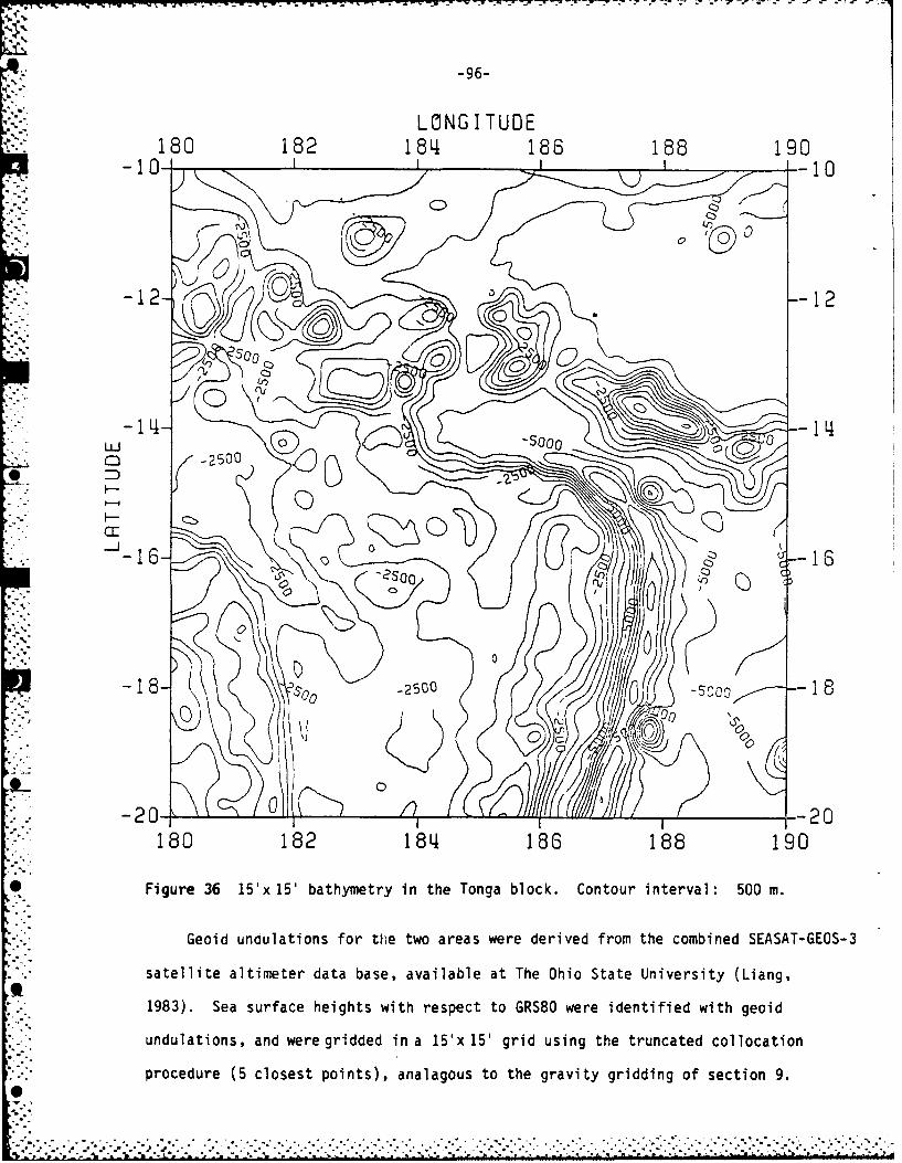
-96-

LONG ITUDE180 182 1841 186 188 190

-10- --10

-1 2- -12

J J~

-1L4LU

-20-180 18A81 8-8 10* iue3 1' 5 atyntyinteTna lc.CntuQ neva:50m

Geidunulton fr ieto area weedrvdfoCh)cmie ESTGO-satelit alimetr dta ase avalabe a TheOhi Stte nivesit (Lang

001

P. -. Figure . . .~. t A.- .36 15' 15 bahme r in th Tog blck Cotu inevl 50 m.k. .~. . ..

-97-

LONGITUDE

210 212 2114 216 218 220-10- --10

0

C> 0

€-'J" 16- _ ,16

-20-u

210 212 2141 216 218 220

-Figure 37 15'x 15' bathymetry in the Tahiti block (Tahiti is in lower left andthe Tuamotu Islands are in the center). Contour interval: 500 m.

The obtained altimeter geoids are shown in Figures 38 and 39. The correlation

to the bathymetry is obvious in both cases, the Tonga Trench having e.g. an impres-

sive asymmetric negative geoid anomaly of nearly 20 m, whereas the islands have

associated positive geoid anomalies of some meters. Degree variances, power spectra

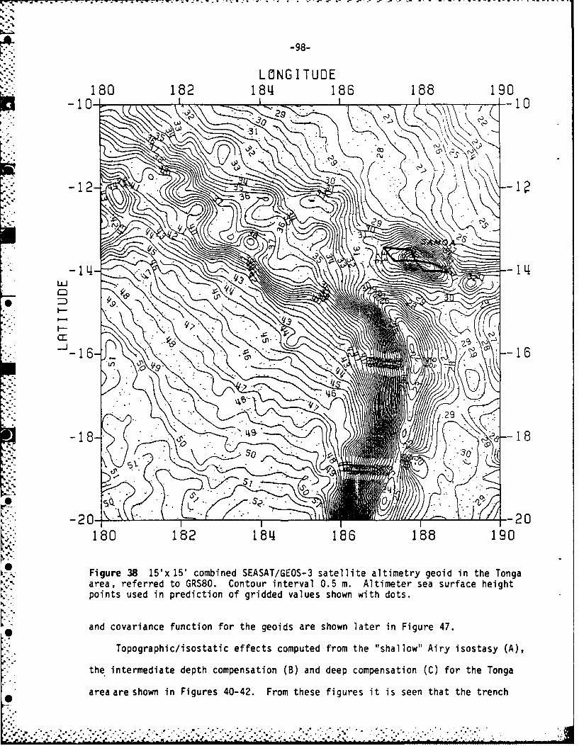
-98-

LONGITUDE180 182 184 186 188 190

-10- --10

29 -..(A)..-,12'

06

18 8214 186184916 --.-1.63

-18 "- -- 18-' "

SS

-20 ...- 2

180 182 184 186 188 190

Figure 38 15'x 15' combined SEASAT/GEOS-3 satellite altimetry geoid in the Tongaarea, referred to GRS80. Contour interval 0.5 m. Altimeter sea surface heightpoints used in prediction of gridded values shown with dots.

and covariance function for the geoids are shown later in Figure 47.

Topographic/isostatic effects computed from the "shallow" Airy isostasy (A),

the intermediate depth compensation (B) and deep compensation (C) for the Tonga

area are shown in Figures 40-42. From these figures it is seen that the trench0T

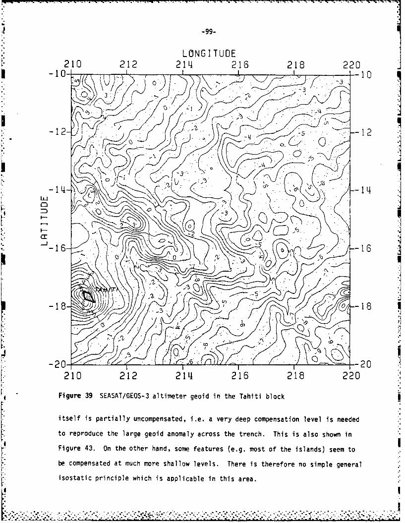
j -99-

LONGITUDE210 212 2114 216 218 220

I -10- -- 10

-2 o - - r7 ..- ' .- . - -o

.1 2. --

214 2-18

0)0

F-2ia

20 21 11 21-2820

Figure 39 SEASAT/GEOS-3 altimeter geoid in the Tahiti block

to reproduce the large geoid anomaly across the trench. This is also shown in

Figure 43. On the other hand, some features (e.g. most of the islands) seem to

be compensated at much more shallow levels. There is therefore no simple general

isostatic principle which is applicable in this area.

• .I . . .- ' . ,"-" . - . . . -'-. . . - ,.Ci , ; - , . """-"""-""'-''""". ..- •"'"""".o.. -,"- -.-.. '"',., '.-.-.

-.. ,- . , >.r. .- . _t..A - , " " - ", - "., " , ,.- P L A,,.. i ,,....,, ,.., ,.,,.--. ,, g, i,,,"...' '." ,' -' , ,, _._x ".

-100-

LONGI TUDE180 182 18~4 186 188 190

-10- -10

-3<" (-12-11_ -12

-1144

*L -20

CI

F1gur 40 0ssai gei-A-nte1og6ra onetoa iy say(oe

Firgthe TahitiblockganiexamplenofhanTisgataticgeoidenderive firyom tbthomer

is shown in Figure 44. By comparing to the satellite gecid (Figure 39), it is

seen that the central Tuamoto Islands area is well represented by the conventional

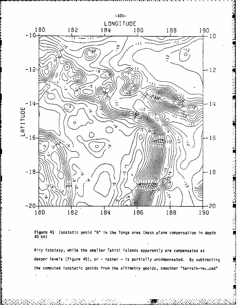
-10 1-

LONG ITUDE180 182 1814 186 188 190

-10 -10

00

-1 - 19

I.-9

LU -16

-20-

180 182 1814 186 188 190

Figure 41 Isostatic geoid "B" in the Tonga area (mass plane compensation in depth40 kin)

* Airy isostasy, while the smaller Tahiti islands apparently are compensated at

deeper levels (Figure 45), or - rather - is partially uncompensated. By subtracting

the- copue isos.*-. geid fro th *lier geis smote * rri-re *- c

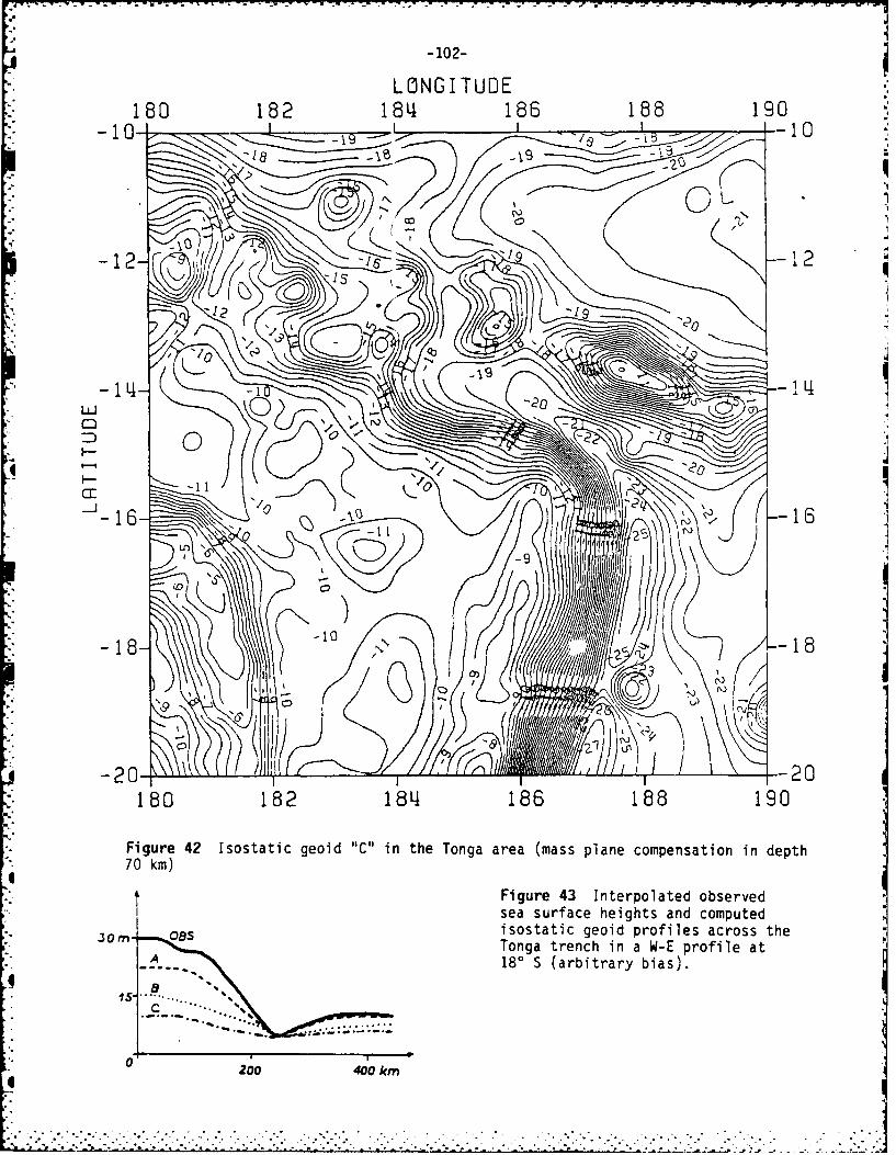
-102-

LONGITUDE180 182 184 186 188 190

CC-12- \--1

-j~

-2-16- %(" -6-- >-9

-20 --20180 182 184 186 188 190

Figure 42 Isostatic geoid "C" in the Tonga area (mass plane compensation in depth70 km)

Figure 43 Interpolated observedsea surface heights and computedisostatic geoid profiles across theJorn- as Tonga trench in a W-E profile at180 S (arbitrary bias).

aP.. . ..

200 400 km

4 . 7 ' " ' ' ' " ' i ' -.-.' ' ' --" . ... .. -.." ..." ' " . - " - . .' ' ' ' .' . ..' .." ." " .' . - -." " - .-.

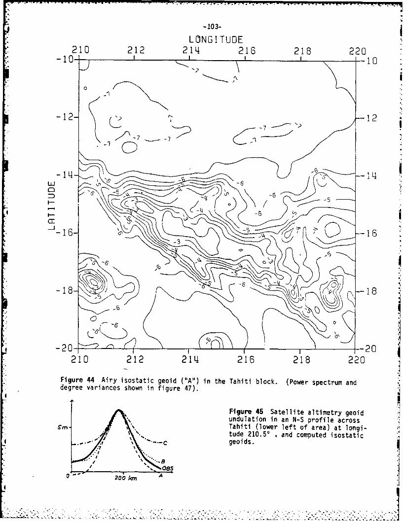
"ON - - I- ,- . .. .- . -, - .IL - ., -. - -| 7- -•- -I.. .. . . -l KI -I .l _, -q -

-103-

LONGITUDE210 212 214 216 218 220i- -10

~14

-12 - 12

-7 -0

_ _ _1

CD

:F-

-- Z Qd- --

<~ 86

- ' 20

210 212 214 216 218 220

Figure 44 Airy isostatic geoid ("A") in the Tahiti block. (Power spectrum and .degree variances shown in figure 47).

Figure 45 Satellite altimetry geoidx undulation in an N-S profile across

Sm- .Tahiti (lower left of area) at longi-N .tude 210.50 and computed isostaticgeoids.

200 A

44

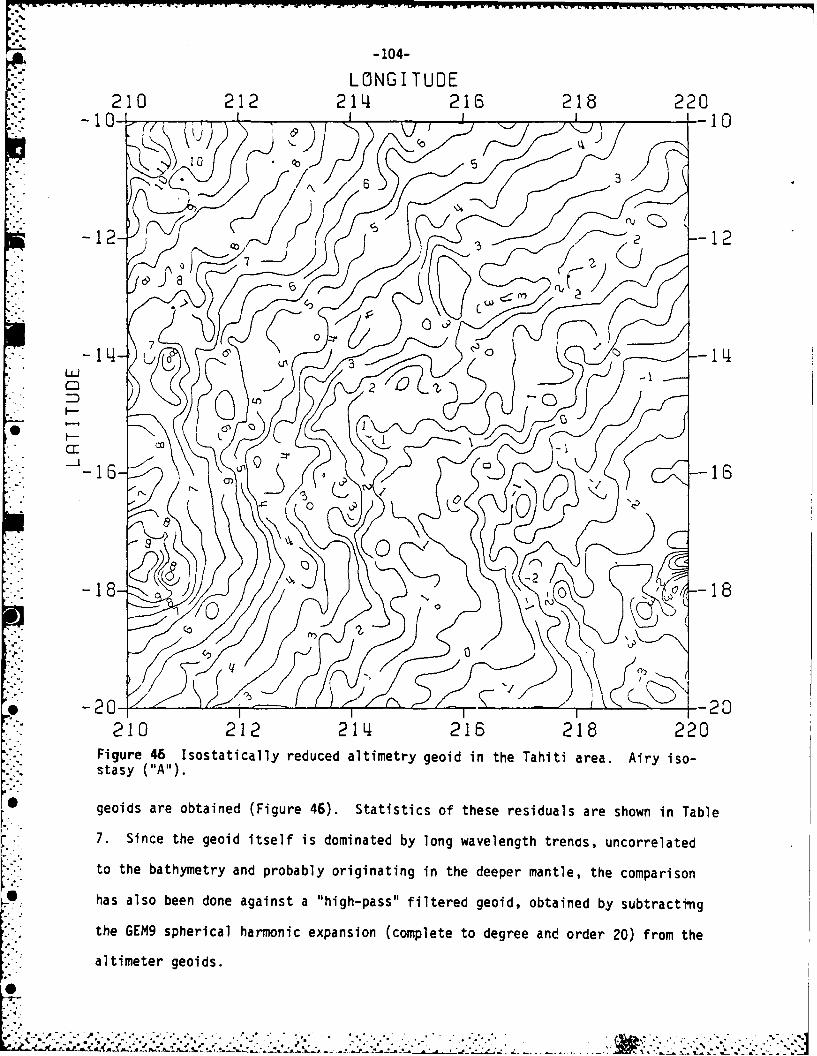
-104-

LONGITUDE210 212 21L4 216 218 220

-10- rJ. j2--10101

N? 6

-12- C -12

Ul 3 -1

D

"" 2 0 22 10 1 6 1 2

16-

0 -20

Figure 46 Isostatically reduced altimetry geoid in the Tahiti area. Airy iso-stasy ("A").

O geoids are obtained (Figure 46). Statistics of these residuals are shown in Table

7. Since the geoid itself is dominated by long wavelength trenas, uncorrelated

to the bathymetry and probably originating in the deeper mantle, the comparison

has also been done against a "high-pass" filtered geoid, obtained by subtracting

the GEM9 spherical harmonic expansion (complete to degree and order 20) from the

altimeter geoids.

0

.o. . ...

.' •° e-° "° j - -o w• ,- . o P " -" " oo

•° ,°

•' " " ', ° ' -. " ". " " .

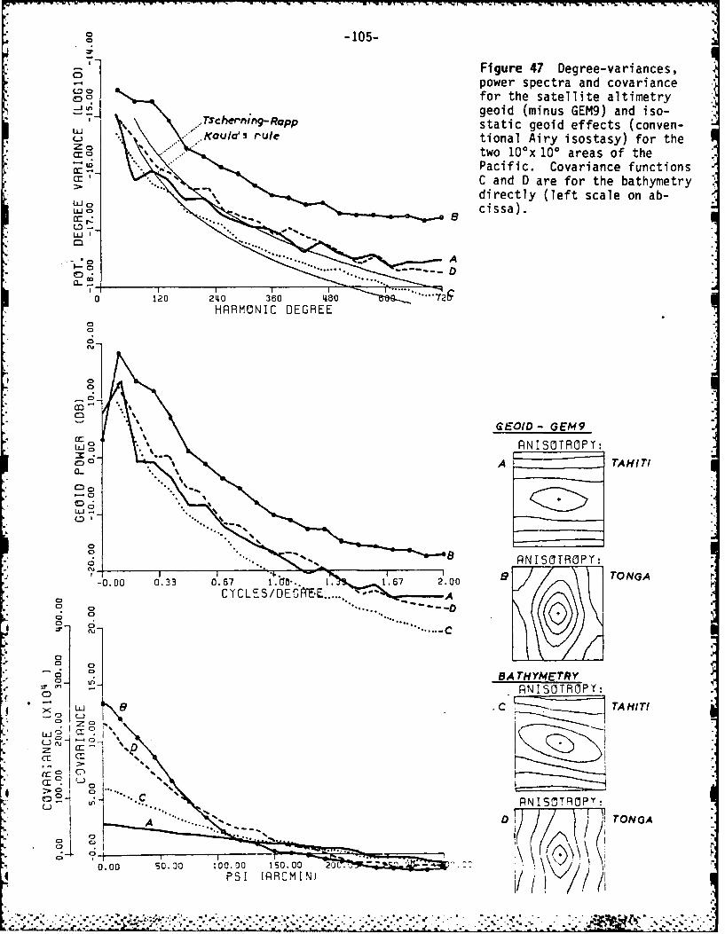
-105- s

E3 Figure 47 Degree-variances,power spectra and covariance

* for the satellite altimetry* geoid (minus GEM9) and iso-

IU .Tcherning- Rapp static geoid effects (conven- *

* .. Koulo's rule tional Airy isostasy) for theZo

CC two 10'x 100 areas of thePacific. Covariance functionscc ~ C and D are for the bathymetrydirectly (left scale on ab-

..U. e cissa).

CD-

0120 2110 360 L&60 _7S~HRRMONIC DEGREE

0

0U

GEOID - GEM'9AN ISOTROPY:

A TAHITI

CD'

M0

a RN ISOTROPY:

-10.00 0 .33 0.67 1 . CTh. 1.. 1 .67 2 .00 TONGA

0-

z a3j ac

Lu%

CD

Cr

CD f RNISOTROPT:

A TONGA

. 00 50.00 100.00 1-50.00 2 0C. -

* ~~~ .-... ~ ** * * * ~ ~ * V * * * . . . .

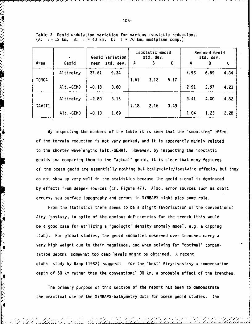
-106-

Table 7 Geoid undulation variation for various isostatic reductions.(A: T- 12 km, B: T = 40 km, C: T = 70 km, massplane comp.)

Isostatic Geoid Reduced GeoidGeoid Variation std. dev. std. dev.

Area Geoid mean std. dev. A B C A B C

Altimetry 37.61 9.34 7.93 6.59 4.84

TONGA 1.61 3.12 5.17

Alt.-GEM9 -0.18 3.60 2.91 2.97 4.21

Altimetry -2.80 3.15 3.41 4.00 4.82

TAHITI 1.18 2.16 3.49

Alt.-GEM9 -0.19 1.69 1.04 1.23 2.28

By inspecting the numbers of the table it is seen that the "smoothing" effect

of the terrain reduction is not very marked, and it is apparently mainly related

to the shorter wavelengths (alt.-GEM9). However, by inspecting the isostatic

geoids and comparing them to the "actual" geoid, it is clear that many features

of the ocean geoid are essentially nothing but bathymetric/isostatic effects, but they

do not show up very well in the statistics because the geoid signal is dominated

by effects from deeper sources (cf. Figure 47). Also, error sources such as orbit

errors, sea surface topography and errors in SYNBAPS might play some role.

From the statistics there seems to be a slight favorization of the conventional

Airy isostasy, in spite of the obvious deficiencies for the trench (this would

be a good case for utilizing a "geologic" density anomaly model, e.g. a dipping

slab). For global studies, the geoid anomalies observed over trenches carry a

very high weight due to their magnitude, and when solving for "optimal" compen-

sation depths somewhat too deep levels might be obtained.. A recent

global study by Rapp (1982) suggests for the "best" Airy-isostasy a compensation

depth of 50 km rather than the conventional 30 km, a probable effect of the trenches.

The primary purpose of this section of the report has been to demonstrate

the practical use of the SYNBAPS-bathymetry data for ocean geoid studies. The

.. . , , , . o . . • . • . . , .I. , " . - % - . -

I

-107-

primitive approach taken here should be improved for future studies, and of par-

ticular interest would be to utilize the global coverage of the data to make a

comprehensive analysis of global oceanic isostasy, e.g. through the use of empirical

bathymetry (geoid transfer functions), class:fying different tectonic ocean areas.

Results of such an analysis could then be used for the important "inverse" problem -

to determine bathymetry from satellite altimetry in unsurveyed areas.

11. Summary and Conclusions

In the present report, many different tcpics have been treated. In spite

of the somewhat diverse composition, I hope that the reader still has felt some

kind of continuity in the contents - the idee was to provide the general background

of gravity field modelling using topographic/geologic information, stress the

similarities to and possible uses of geophysical inversion methods, stress the

practical benefits of using spherical harmonic reference fields and then finally

go into details on terrain reductions and prcvide the theoretical background for

the FORTRAN programme published with this report.

In the first part of the report (sections 2-5), the necessary theoretical

background was outlined, including the concept of density anomalies. Opposed

to physical densities, density anomalies attain both positive and negative values.

In spite of the basic ambiguity of potential field theory, it is still very meaning-

ful to work with density anomalies, even without having defined the "normal" density

distribution explicitly: it may simply be taken as an average "expected" geo-

physical model.

Known density anomalies - topography, isostasy, geology etc. - may be taken

into account by a "remove-restore" technique. Then values of anomalous density

etc. are assumed to be known. For unknown densities, geophysical inversion

methods may be used to provide better models of geologic structures or to provide

. . . " - " " . - . " - . . , . . . "- . . - -. . . . . .. . . ... " o ° • • -,°,4" . "" - , . t ", , . " _. ._ . '.,., . .- . .- , ... m -' ' _.

'Q -108-

"optimal" density anomaly values, e.g. finding a best density for terrain reduc-

*tions. Furthermore, it was outlined how the "ultimate" combination of generalized

inversion and gravity field modelling by collocation in princtple could be done,

*' to allow incorporation of e.g. "non-gravity" geophysical information in gravity

field modelling. In the second part of the report (sections 6-7), emphasis was

on terrain reductions. Formulas for the gravity field around the rectangular

prism - the natural "building stone" when elevations are given as digital terrain

models - were given and evaluated. The.basic "types" of terrain reductions were

then reviewed:

- Bouguer reduction, removal of the visual topography

- Isostatic reductions, removal of the visual topography and the isostaticcompensation

- Residual reductions, removal only of the short-wavelength, "noisy" topo-graphy

The terrain correction, frequently treated in the literature, should not be

viewed as a terrain reduction, but rather just as an important mathematical

auxillary quantity. The programme "TC" - given in the appendix - may be used

to compute any of these types of reductions for gravity, deflections and height

anomalies. The development and implementation of "TC" represents the bulk of

'practical" work associated with this report.

For error studies and FFT-methods, an approximative terrain reduction for-

mulation - the "linear approximation" - plays a key role. The accuracy of the

approximation was investigated both for a theoretical model and for actual data,

with the conclusion that the approximation is usually acceptable. However, care

0 should be exercised in alpine areas, especially for deflections of the vertical.

Assuming the validity of the linear approximation, effective FFT-methods

for terrain effect computations were outlined, and finally a key topic - DTM

resolution requirements - were studied. Curves were given to compute r.m.s.

errors for terrain effects for gravity, deflections and height anomalies, based

on spacing of the given elevations and on topography covariance functions.

i

>7 -. P :.- *

-109-

Finally in the report, empirical data were investigated, to give actual

empirical information on

- topography covariance functions for various types of areas (they turned outto be generally exponential)

- magnitudes of terrain corrections

- magnitudes of RTM geoid effects (they are actually so small that theindirect effect on gravity anomalies may be neglected)

- degree of smoothing obtained using terrain reductions for actual gravitydata (as expected variance decreased, correlation length increased andanisotropy was diminished)

- relationship of altimetry derived ocean geoids to geoids computed solelyfrom bathymetric data (including bathymetry covariance functions).

The main empirical results - covariance functions for topography and gravity -

are contained in Figures 23-24, 33-34 and Tables 4 and 6.

Unfortunately the duration of the author's stay at The Ohio State University

was too short to allow the implementation and practical evaluation of some key

topics of the report. Therefore, natural extensions of the present study would

be

- implementation of hybrid geophysical inversion/collocation, with test inan area of well-known geology with large density anomalies, e.g. a salt-dome province, shelf area, etc.

- implementation of a "hierarchial" FFT terrain effect computation system,with comparison to results e.g. obtained by "TC" in a suitable test area.

Other directions for future research could be the extension of the analysis of

the covariance functions for topography and gravity, to include more regions of

different types. Ideally, a classification of "covariance provinces", based e.g.

on existing geographical landscape classification systems, could be attempted.

The availability of the global detailed bathymetric data set SYNBAPS opens

as just mentioned possibilities for extensive studies of the relationship between

the ocean geoid and the bathymetry. Ocean isostasy could be studied for many

types of areas through (FFT) cross-covariance analysis. With the results it

could then e.g. be possible to design optimum filters to derive the bathymetry

a

-110-

from satellite altimetry in poorly surveyed areas. Another application would

be to "enhance" geoid variations not associated directly with bathymetry, such

isostatic geoid anomalies being obviously of great interest for geophysicists.

F2.-- , 2.

APPENDIX

TC - A Program for General Terrain Effect Computations

The terrain effect computations mentioned in the present report have been

done using the Fortran Program "TC", outlined in the sequel. This program - which

is written in structured Fortran (FORTRAN 77) - has been developed and implemented

at the Amdahl system at The Ohio State University, and has been tested against

"synthetic" topography (cones, cylinder segments) and results from an older, some-

what different ALGOL program at the Danish Geodetic Institute.

The program uses a set of digital terrain models (DTM's) to calculate gravity,

deflections of the vertical or height anomalies at specific points, using the

formulas of the rectangular prism, outlined in section 6.1. Four different mass

model types may be specified: topography, topography and isostatic compensation,

terrain corrections or residual terrain effects. The computations may either

be done out to a certain distance R, or a specified fixed area may be taken into

account. A fixed density of 2.67 for the topography (h >O) and 1.64 for the bathy-

metry (h<O) is used presently, but it may be changed easily in the start of the

program. For the isostatic.compensation, an Airy isostasy with Moho density con-

trast 0.4 g/cm 3 and normal crust thickness 32 km is used, in accordance with accepted

"best" continental values.

The curvature of the earth is taken into account to the second order, through

the use of the "super elevation".

SUPELV = Rearth

which gives the z-shift of a prism in distance s.below the tangential plane at

the computation station S. This approximation is valid for distances up to several

thousand kilometers. The superelevation is also utilized for terrain corrections,

so for very large computation radii terrain corrections must be combined with

4.

-112-

grid

A 1 1I Ai

- - -~ - -,

. --=7--

Figure 48 The use of the two DTM's in "TC" terrain effect computations. Elevationsfrom the detailed inner grid is used in the outlined rectangle covering the circleof radius R,, centered at the computation point S, the coarse grid being utilizedoutside this rectangle. In the inner-most 303 grid elements (the "inner-zone")the digital terrain model may be densified using a bicubic spline interpolation.

the spherical Bouguer plate formulas rather than just the plane formula (2TrGph)

to give the complete topographic effects.

Two digital terrain models are ordinarily used for the terrain effect computa-

tions in "TV" (although both are not necessary). A detailed grid (say 1IkmxlIkm

point elevations ) is used out to a computation distance R1, and then a coarse

0 grid (say l0 x10 km mean elevations) is used for the remaining "remote zones",

see Figure 48. A distance specification R, of the order of magnitude twice

the outer grid spacing is usually sufficient. In addition to the "detailed" and

"coarse" DTM, an additional reference DTM must be specified for residual terrain

reductions. This OTM is used together with a parabolic hyperboloid (bilinear)

.,'.interpolation scheme to define the mean elevation surface.

-4L- -

0C

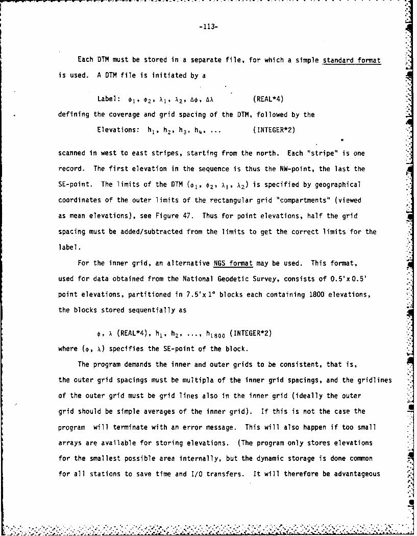
-113-

Each DTM must be stored in a separate file, for which a simple standard format

is used. A DTM file is initiated by a

Label: 01, 02, X1, X2, A0, AX (REAL*4)

defining the coverage and grid spacing of the DTM, followed by the

Elevations: hl, h2, h3, h4 l, ... (INTEGER*2)

scanned in west to east stripes, starting from the north. Each "stripe" is one

record. The first elevation in the sequence is thus the NW-point, the last the

SE-point. The limits of the DTM (01, 02' X1, X2) is specified by geographical

coordinates of the outer limits of the rectangular grid "compartments" (viewed

as mean elevations), see Figure 47. Thus for point elevations, half the grid

spacing must be added/subtracted from the limits to get the correct limits for the

label.

For the inner grid, an alternative NGS format may be used. This format,

used for data obtained from the National Geodetic Survey, consists of 0.5'x 0.5'

point elevations, partitioned in 7.5'x1* blocks each containing 1800 elevations,

the blocks stored sequentially as

0, A (REAL*4), hl, h2 , .. h1800 (INTEGER*2)

where (0, A) specifies the SE-point of the block.

The program demands the inner and outer grids to be consistent, that is,

the outer grid spacings must be multipla of the inner grid spacings, and the gridlines

of the outer grid must be grid lines also in the inner grid (ideally the outer

grid should be simple averages of the inner grid). If this is not the case the

program will terminate with an error message. This will also happen if too small

arrays are available for storing elevations. (The program only stores elevations

for the smallest possible area internally, but the dynamic storage is done common

for all stations to save time and I/O transfers. It will therefore be advantageous

71

, . .. . .. . . .. . -. . . . . .. F . ...2. .o . . .o . . . . . . , . .. . . .. . .. : . . . . . ., . .

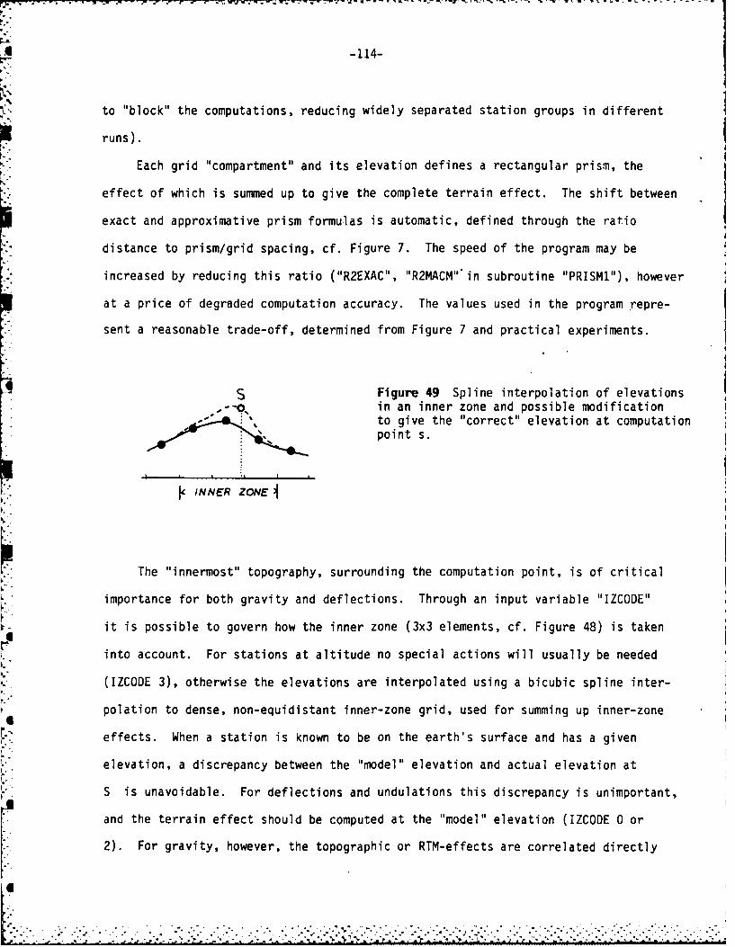
-114-

to "block" the computations, reducing widely separated station groups in different

runs).

IC. Each grid "compartment" and its elevation defines a rectangular prism, the

effect of which is summed up to give the complete terrain effect. The shift between

exact and approximative prism formulas is automatic, defined through the ratio

distance to prism/grid spacing, cf. Figure 7. The speed of the program may be

increased by reducing this ratio ("R2EXAC", "R2MACM"'in subroutine "PRISM1"), however

at a price of degraded computation accuracy. The values used in the program repre-

sent a reasonable trade-off, determined from Figure 7 and practical experiments.

I SFigure 49 Spline interpolation of elevations

- in an inner zone and possible modificationto give the "correct" elevation at computationpoint s.

I__ _ _ _ I .

INNER ZONE

The "innermost" topography, surrounding the computation point, is of critical

importance for both gravity and deflections. Through an input variable "IZCODE"

it is possible to govern how the inner zone (3x3 elements, cf. Figure 48) is taken

into account. For stations at altitude no special actions will usually be needed

(IZCODE 3), otherwise the elevations are interpolated using a bicubic spline inter-

polation to dense, non-equidistant inner-zone grid, used for summing up inner-zone

effects. When a station is known to be on the earth's surface and has a given

elevation, a discrepancy between the "model" elevation and actual elevation at

S is unavoidable. For deflections and undulations this discrepancy is unimportant,

and the terrain effect should be computed at the "model" elevation (IZCODE 0 or

2). For gravity, however, the topographic or RTM-effects are correlated directly

-115-

with the model elevation, so in this case the terrain model should be modified

to reproduce the elevation of S (IZCODE 1). This modification is done smoothly

within the inner-zone (Figure 49), assuming the discrepancy to be due to erroneous

(biased) DTM elevations. Since the physical mass model is changed independently

for each individual station, some care should be exercised when using this option,

especially for large values of the DTM grid spacings.

In the sequel the programme is listed, more detailed information may be found

in theintroductionary or "en-route" comments. The programme is modular constructed,

with subroutines "TC" giving effect in one station, "DTC" effect for one grid-

compartment and "PRISM 1" giving prism formulas. Station input/output should be

modified (in the beginning of the program) to satisfy the particular needs of

the user. Typical computation times at the OSU Amdahl system is around 4-5 points/

second. An input example is given at the end of the program listing.

gI

-M116-

-~ ~ -Z 4'iW -ZLI~~~~.xc C:, 04I * 4 L 4

-0 *. 44W q. 00 0 .0zN I

UC.w - OC UWZZ*U -:

WX -K 0 z4'

cc. 40 w . C 4. 7 0a Cw I.o .- V, . 3i Ix ? Z -4z .

XX~ ~ *.2LO Z 7 4 4.

U . d w , , 0- 44 , -: Z . ,

d_0 a4 xI "I UL ac -,w -:2

-. Z 2.. 3C CJ QW O9 W 4 Z - 0 3 WCL- ~i U- -,- J K .4 c 0 -

EU C.) z~ .9UL- L 0 U 0 k Ca LA. 3.

In 4z 7- 04 z Z 0 CK OC 4.4 L

74~~~~~I .. CO 4 r X 7 U.J.7 ~atU~ .S UW I-2 0 0, zLIW 0-: LI L u~ -

., L VI U 1..3.~ ~ 7 U-

.9 U! *. -4 LI x x ;- 7W ; Ii.* 4 ~ 4U L

LA- U a * W Z Z - L ~ -0J

W~) -4 '.U 0 lu Q~ ~ . -

v il w. ki wLI 4 ZL Li 60 .. 61 w44 4 4 %j w .QwjUww% w w Qww

*4LI~ ~~~ C- .9 0. >LU > 0L7 - 9 Z E

IL an z .. -Z

S~~~~ 0L z Nc 0 .. zI 0

-- .. r4 -j r~ *j *cc4 a. 4 U 4 9C -9 :L W 0 0

4> 00 .4 &7 -A 0 t0M

0 .. Z* 0 . x-9 w. WW -. 4 LI LU ~*j>. .1 4oo LX -o o m 4

-W .90 ,4 .d. * - -

LI XZ jA Z >X -). 4 .0.- ,, 2 - IZ

%I wZC U 0 w r *. I- -LiLIa 0i cc nOL 4 01 007w44 - ^

LI I LI- W, -0 LI 20-X -. ?-w

U ~ ~ ~ ~ 0 - lWw17 .. 40 .-1 -7-

ki w aU -9- LIU- Z-I V Cc44 - 0LI0. -- z :D , 0 D; xi Dj > & - jj7 4

LI - U * .74 0 O ci..O. Li w LU 0037. 40.

U0 g 0 41 0 Z1 7U 'u >> r. t L xU Lic UL cc N. 1 7 U~ U

ALIC LI CIE Q- UK C >j 0Z KULK0 .

Z4OLU9-Zo"I

LI CL a 3. 1 Z U! =I 070 :0 4K -4, M 0 4 W.li aW x A 04.?w .4 a-~ LI74 -m -9x MO U .

LI -0 ~ .d0 II .. - UC X~( LiZ 4.U .1x

LI z;_ , 4 Li W - E O , ;X0 00. .. OZ.fl 1.U

U U Li* 7 W W .4 11 16 WI 40 G*iIUU,

U 0 4-0 a. -4 LU i A .2 W 40 UW Lii14i QS4 Dw ... 0 ILI~ Z 77 L 0i 9 Ji..U -*.4 iW --

IP C0 W .. Z. .L44 LLOiO 4 Li0

U - 47 0 020 9A9. U Q~i~i %~l Li .lL0407Ua.Ii 0 - 0-ILi8 C U E 9 04

U1 w w. %- w wZ w~ 0 A0 QUL % 4 %JJa ww % %

NN

00

- .- w-a -a L)0

a. . u. _j

z 4 cc .1 M9 w..j

0 2-j 1 .. t . 1

4'u 'a~ Uo 'Z o 4o~~~ o0 * 'o4-

W*w4 -394 'A N -w4 _j m.41

- 09 N 4 it NwaZxw 0 Z 7 7 4

N Z N--~ 9- 4 0 6. 4.. Z* o <: A14'943 > 0:! - 1 4 A 4 12 2 -j7N%6 N kw w U. 4 ZOO

ac0-~ er -1 U j . L6 _j. Z4 0. Cc

w. u 4. W.40 04 '. 9 t-,, '. I; 0 x(L.c_cc-2..1 93 0- Z L49 It.99 *z 0 49L.4 %

t 19.- * N '0 E- N cJ - 4 1 4 >. - . '. -9- 7-~~~~~~~ ~~~~ a. a- 4 0 4 9 '4 4 L L 9 - 9 0.-

99999999~ C39. 'A9991 C) r z0 U- - - ~ - 7

0000 o -c- 4- c 0 -w .w.u IZ.1.Zx. ;

9- 9-" w 'cc 410 - oo

4 w 0 *z 0 4UX u9 0 .j- -. 29.. N w 0uN ,

ie L z.' j cI- 049 7W o * ow

'A Ua. u ~ U. Z99 9-9 0- A U L > 0 4

.. -.- 4j m - 0 z 0 Q 0 '0 u -.4 ~ U ~ 4 -x 0 j

U~~ ~~~ 9-u9 Q4 0- 4.9.94 s.. %9j 3 7-- ~ o 7j cl >-) 0 9*. 4d00 ' . .9.

19- 770 - I -'-.09-'.9. 4I - U I- 7 4. - 910 9U UJW9- .91'9 4*'U - z - 0 0 U - - 4 - 9 N 0 9

I- zW '091. UJ- . 99-9 0 U o 0N 21

C.'0. ~ ~ ~ L 09- X- 0-4 00'0 UC3.~ * U 0~~.9-- ~ ~ ~ ' jj.79U - - 92 >' 4 U 4 - Ud0 .Ixw O-0 0 0 cc-** -. -9- 0 7 ' -

0. '044 o '4 a. .'90 97 0 49z ,, -3 w-0 z.- -I X

9- -04 - 9 cg 0 cc W 06-1 CC 4 9-0 U 9-* ( 1 07 46 au.- 0o - w 0 4 9 kaOZ 9 7'9'29 z0 U m9d Q' .. 9 > ac-

w0 UU 09 0c 747 a. cc99 - 0. x9- .0 9xc- D-2a66. Z4 : '9 70 9- W00 -R 0 Uw v w9* 930 .. o9 N41. 9 0 'A 09 c In*, x-2. >.9 U N * -4-

40 -0 9 M 74 4,AU , 2 0u - U oc- m~ .4

0 " x 11 92 24 b- 41J 1J -a 9 U acZ Z*9 660o*'a ,-9 '0 20 w9-9 w0 a09-9 * U 94 I U 3-

04 01 0.4 : -.- A a.- . -o .. 0 M* Ux -t -9 9

9-0 u4 * 4) 04 9- - 0 9- 49 z1 Q- U L 420 a .& x Nz0x-x9-9-~ ~ v-4 A9 m. c2>4 u w99- aU U'A 0 A2 4 0~~~-~ 270- 9--9 9- 9- U -' - %j U *0 I29997 - '4

N9.J9- 7(70 49- '0 .0. 49 4.0 444 9-9.9- W>4~0 91.'In

4 -1*4 04 -0 74-949 4 9-U -> U 9-9- %

9-70 - .4 ~'U 9 091'0 -~ 4 '0Z 4 WO U .~09'0 9- %

9- 79-0 4 Z 9142 9-9- 9-'07U.9 77 U - 4 0 - '

Ny w

a, 0

T I X

de W% cc .4 ' .N 0" I

a.~~U n 0 x

CL -N -u 0

4N2 C NX U,: M. V0

r .0 r: 0 -0. 0* =.NU 0 N ta U0

322 w2 -1 w !1 0 WN - OC K4

. U. iN .0 U. ~ .

~~- 02 30K

:5. .jIN 10U 01. cr w t t?-0-- 4.. 0.u 0 0

X L. . .. 9 Lifx0

-) - 0 4W. 0S w 0 N J0 66*ZA Cox *U0 + K w N - 0

.0~1 A- UN a,- l U

-- 4, ZN.. 0 "o0. 0' .4 4 -l-~~~U.c 0UN -~ l..0.CL-UUZ U N

*~~~ U-U. 4..JU0 K 4-11,1 U1U-4 .J0- Q -- ,N --' N , 5C 4 .. 11 -: -.

£U44 .4j Z- cc 4 0A . 4.U. 4 UN L). CK Q ...

Z000 ~ U zN - 0- cc T 0-UNOUN N .J.

aO0 )O- 61 %6N4N 0 LM N w N W w4 * N

ZUN 0 W.0 0 -00 .A-Z - .4N4U .U - ~ Z-04 *j..

- ~ f V%.lU ... NU 10 -4 4- 1 I" M.N - - N~J .. aZUUU.-.- 0Z ujZ 6.UND 4 49 aU..~).K 0N 4*K~

.00 04 U col 'in ~w U..440N0 01 -. JU ONNNJ.

~ KJ2 ~ %.1IK .4 UN *U N.J2K g.N ~ L*UNO0..

UN* - - NNO~~~~~~~OO N0 XZ C0 N.)4*~.* ~ ~ ~ Zt .. N.I UN -4 N*I NW0. N.2 -U

o ~ ~ ~ U K U.Uk4 N IK

N N9 U N XNA 4 . N

cO ; 00 0.A0 I- Of

Ot IA. JUJ

0, z 0

6. %U.N:5 t ' ::N.A Z .I

Z.N Yu 4 Lz .

9 . D A wc N atU %u4

~~~~ .-. N %N

0.) 0 W S. %0 -0

WUUZ.- U - -

119-

'v* z

ZoC 0 a. ; 0. c-a a, 3. - -J 0000

* 0

110 0 I0 0*WO I- Z *0 X. .- 0

z 0- 0

-0 2P *-0 05 5 3-*o CIL0 Ie. Q0

at !9 2 IA9 I@ Q

4wo * 4 * *

*0 j 0 OA400 0 *

cc (4U N - 4 00l at cc w w 9il-e - W 16 %% J %. .9 449

0 It~ -, 0 -- 8 JO

- - z -lw a. 4 -e j

a4 a - ... ? 0xX lU .44 I-8.a:!

0 0 UO vi w0 0 NN ' %%0 9 -t A z -WI 00'1 111 cc4 at cc40 M %.J

- ~ ~ ~ ~ U .- w ~ z - .- 0 *UW 244 4 - - -2~ ~~~~~~~ K Z C -52 U g l

(.2 11444 13 1%,. - - 4 eI I i 0 .

wt 01 Q j O 0 % O . 13 612..4 1 I U 2

~~w w v 0- %a. Q4. - ~ 1. - - - 4 4 4 - 4 -

IA ww u 0 N 81.4- 3 - - - .1. .

4 4 14 N4 ~ A'dd 0 14 4 U U - - - 41 44 ' 0U **. ~ 0 44 IA- -40 -4 .11100 444 JU~JU 0 - - U Z

-~q ly 0 W h 4 1 4 4 2 4 4 0 * J2~~ a. PC0) 1 4 01. OAJ1. A 1A8.. 4 4 4 .a~~L -. 4 WNOWIIZ % I II W O - - -1.A81. . 4U~~~ ~ 8.. -. *' fy N - - - - - - - - - -

000 ~ ~ ~ ~ ~ ~ ~ -2 WU.40 4 O NN 4 2Z -4 '. 6(.4 .~W .. 44 8.. 4 4 4-4 ~ . 0.

0~, r4N - Or0w01 - - - 0 4 2 4- 4 N N - *

IA~- :44 I- wOA 031 W W N NN .9 - A

%J t

00

UUUUU! 14

U U -It Uit U N 0* :

X; U U 0 -- v U0 1& U. %.N .-~ U U ; N

4 Uj u , CC;= IUO 4 -1 .28 4zA U 0 -w~ a 9

N %J w I * 4

Vi U. UU. 01.

1, 0 UJ Uw ? AA "1 U2 -C U z w 2w-z I U - U z C6 W %21 4.3. 0 'A x

- U 1 4 z 8.Vi0 4~ 04ou U Wi U9 :) ; UI !. 0% U

Vi t U -0 U4 u w4 04 ** 4t cc I.4 -

Q w - - axa ai U a U; IL "4 1 01 4 4 0. 01

wi. 44 U w U 0 u a 0 U N %m120 w4 z 1- 0 U N N .N. * - 4 *I .1

0. U U2 W0 !I 002 .2 0 .4 2 .4

v Ni 0- U0 -9 U9 'A a8 39V 0N4 4 x1N 1

w 2818 41.2 U. -0 A W 06 %a C %A .1 W 1V -4% 0 'A kAA

I"4 0 3 U U U 4 6 .2 4 W 4 O . - *jl~ - 4 U 0 4 U 41 00W N4 8.8 l24 *

-120-

7 7 W -

I- --

Kx 3- 4 a- I

W, 0 -oc t 0 W% 1. 0

-- D CL -1 x C;

0' CL IL 0 0. -

*I -C j z -A a N

4 W 0 at - -a U. -. 00 0.4 -, u Z U. A 0 4 0 N .N o U N

*l %4t -0 Q x '- CI 00 -0 0 0 -- 0 i 0 000

IA~~0 9o %jI a zb % 9 O

-0 z. - 0 -A J

2~~~ - z. 4 2 900 P.- CV.4 > - 9- 90

2 - !' 1! -6 --~% P.- 4 - . j O - *II 24 - .d -) 9I &~ ~ vO ~ 2' N 0I9

IAI- X. Z x0i I 9 W U M . 0 * -

I1 I- 90 O-Mj Co. we 0 W 031 Q 00.2 - A .3.~ UA -9! 0 b6- 59 7

2~1 -9 1 A Z 7 Uow1..)I 2 L ~ I . 1 -q -Iu-a2 ., .j N4 N = .i

of 0 2SZK 0 I * -4 o K. s

0 U . 1 0 1 -U. N 1 -. NI;;:cc I .- v IA cc w 0 N N %N N i

Lu44 -U 44w144. 11 .. ==a.4

NNNN . W. 4 j .

-M-0o

0 02

* *Z - -

U. C

Li mi U. w I

li w at 'A UA W or

42 0 -4vL .1 OWW 0

U.-a.~ U. 0 .

NI CL - %!- LIU9UL=00 %6 N I. U 0-

wI C, 9

LI :2 w V.4 0 -L U. -.LI- x N W I& LI f I ILI

LI CIE 4 K 0 > V. 4 wI wLIMccb c e

LI W WI 0-v . , I^ - 2LI "I a W U. z 13 A O v

LI-~~~~ LIC4* U -UILU 4

LI4 - r4 2 2 7U

LI N o ~ v U . - 40 I0ULI~~~: 9 I 0 L - U 0 LIt

LI cc z ti.U cf K i .4 a 1 - U0oCL I w 4 0 IU- G "0' 4 L 9 -

LI (a 0 0 2 W0.. S 1- LI ).- I f 0 - 2LI a, I ac' aUL I . 61 VI = .J -a x 12 4

LI CIOJ zU z Z I LI XL - IW U. U.U.±I t0 a aI 'A U' CL %6 416 W -9 0 X LU. -. '

cc 4 LI.ILK0 X LI9- A Z. U.U L - I 4

LI U1 z LIZ 2 at L.UL LI Ai j.A z 0 -.a0LI - 0 0-L U 0 ~% w - I 4 N . i O L . J

LIf > J.04 W X. 9 U. LI- WI NWi. . C 0 - ~LI If If Uj U. w. W - L W 0 0L . Z I .

LIl~ L. 4 i L .J * 0 U 0K - 1 . A . L

LI v 46L0U2 0 16.11I N L L - I .- .. ZJ

LI - - 2 % - LI 09 I 9- 9-94- . LI j * *C

LIc %16 u-U 3 9 i A I . . J U 4 W I I Z JLI1 f I 0 Z Z Z I I . -- - . W L v 9 U I l . v L - L

LIc aU K 0 Z U I U U. I .iii 2 4 Z U X . i Z.J 0 L

LI0 ki L

LI,

3. U. a, LI% UI LI LI - IL

. U .IL

- 0 16 W UL

% 9- 0.- b - LI

3- 3. 0 LIW QC. 0% A. IV U" w. Uc LI

3. - I . 0L

I - N N IA 3c 0L L

Z ~ 0 .0 U. all WLa 0 LI Lfy 9- ).) ). -L 6 I I 0 .

LI4 - LI ,LICI%49 U Q 000L . 0 LIC 'f6 J. -1 o Z cc K I

d R- LI4 = LIO- cc q 0 LI W;;L L

W o caN W. IN .- 9- L .O 0L ULI ; 40 1 9 - * US . I L U L I L

- If9 66 9 , 9- 0 LI 2 UUL 0 U-r -a 09- w- e9 LI wA .4I0UL

N - *N .4 9 0W *N -- LI LI wc 16.14IU 00 000 9.9:z 9--. *-0Q4 .4 .0 .LI 0 *LI 0

at9 3. -9 04 93 0-- W L K - U C. 9-L

116 9 I OW O LI LIL 6 WIA V LI w. I I LU6 IUUU3UI Z90 0 69 4 9 L W w LI A" LI. IL0 *CU W log S4W O I L . 9 I . * .L ICI L 6 ~ -4 0 0 * 6 I U 0 U I

- ~ ~ ~ ~ ~ W UUI W42 W4- 4 WWW2 0 W 4 0 WWWLI U

0 * N4O .49 IU I*004 0 LI .UdLI4 LI - WU I L

-122-

K4 0, at4

z z

"i jo 9Or a 4 4 C

3-3 3c L2 4 0A 1" 0 00

N49 C M Icc ca 0 44 U N Q NA

0~ ~ 4 9 0

K '9 m 44 " * "z 4W No 4 - X* ry Ny FY N4 N

0 XQ 4 K 49 IA 4 0 -jC" -9 zNXc,A a lU 9 4 -4 )K 0 I 6wW L- X3 .-

'A U. 4

4 z 4 44 -D N&U; - 01. 0 4 -

K 4 4 04 ^ ; N- N0N ~ ~ ~ w n% 96 - *

*~~ ~ l Kz z2 4 * 44

N ~4 4 4 XX a U4 U

CU~a UU 4 0 4 4 CC

). -~ K 1 4 w4 4 - LCI~ ~~~ ~~~~~ 44 m 4 % ZU.3 4* *

0~~~ 4U2'91 IK0 4 4 N Z 4 4 K % *~ s

fy KA 0 %a U*9.I AA KK TK0- *0 -c

0* 0~99 -. z 4 c4 A - I

I 4 9-9-0 4 9 N U AfQ 0N U, I. 0w Uax

449.- %J .3 izo9' u9. U Z44.'AN

K 2; 0 0CL W ft 'A

a Li9 dc U9 e

*A UA II X -z

= x ZTj0-:1 WUrQV; -4 I

U6 XW UA IW c - U0

XA Ui N, U. (A 4 .UD .- LU 'A U Q- T -a,

0 NA UX 4UK U'l 49 U, -C -- 0 UIA.

A a U -. U 4 9 I N 9 aL* a - cc U 43 U w - LS ( 04 -

w NA I4 U N Ut fm - 4 9 00 ~i NA U. -6 4Ua U 'A

4 oz NL N -j U! w ,38 U Z b, 4L .4 A0#M PA di U . IA ZWW U91 %ja Z 0 %A K

4; a N 1 U .40 i 0 U at j 0

N 06 IA 0 U0 P4A U .1 WI 06C u .at& C co - - U: 1" -j 16 U v '0

-1 4Q 0og U0 401w UU4

M.~ d a* U W 11 U K WN

-~~ 0 VAZ U * 0'-'~~~% 0 W , N W K * 0

-123-

0

LIh at WO 24

LI W I 41 NW4 .9 orILI I -0* x0~ .0 0L t; 2 -LI o 4 I u.W Z 0 - 0W

LI ~ ~ 4 0 0 A 4 f C *W;. I W WLI 4 o I 1 0.N0 4 4

LI Om40 2 022-- L . O%j 0 OAWN 4 0-4X 0 3C V.i 4AL v-

LI VI w4 L < J - 4W 4 4 W 4L Lcc I. -- o-z 0'AZ wj z a ~ -

LI LI !KS-I.- WC- LIS 1. 4 Z d. w 3

QI 24 w A WWIal-oi 4 s ., W: ; - 04 0,WI 04 - &.3 0w4 w44 -w 0 W L UZ C.9 -CW W m - . a Ljwez45 0 LI- W4 -x w 0 w XLI >- La

WI 4w u WC544 W.1 aO- ki j e Z 09 o-.LI "-, z t 0 W 0 WJI L 0 -l r WC4QI OLI LI LI 4 q Lw - %W U0 w I 0 L -* LW

L .j0

"3 ~ zL w 0~f --CwL W. LI N I -0 '^ . .LI!4 WC V, 3 L4J U'SI 5O 4 0-1 0d t- w LI OZ wt ~ I

wI v 3 -WL ZI4I5 aA 0 Cc CL LI w OA w w 4

tJ ZL U 0 . W 5 00 cc LI -u at u W.U 0 1 w LIaI QI 0m W j4(.4 0M uw- & 4U 0 c - 1 >L S

LI 0 EIz U~u -. W IZ C z XI 0 mI w 0 .LI L

CL -. wtwXI 4 - ~ O~ - 2 L 0 C3 0. LI.WLI .Xw LIZw04 .!O.lc 0L~tL 09 40 0l 0u - . 4 t 4 0 LL

LI w4 WI LILIOLL cc 4O L cc w W. 0I at w x w z z0

WI U.I 44 N-4 4 .

2I z "C -0 -4 - .aLI La. . - z A0 --0 . -I

LI 20 .4 ,, 00 1-

LI 0 > 4 A O- -Ut 5 I - UtLLL 40 3 w t w Z . * 4 - . .-

LI 4M LI C 2 - -L25

LI 0 LI - 0 - - C C - I I. 14 4ml

LI U~t I - C - I - U. C Z -ZI19

- - N

q Q -Q Q -409 L

N - 0 4 ii - -: U x

0~ xUt N - N N N

4 owl*4 a - a

I ~ ~~~~ -.- - - 4N 4a

z. C 0 x- W. 0 M :01 1QM4 2* U.N SN 5-NN

Z --- W -%6 "4 Mo NJ -. -- tw 0 'A 4 4L 0Z It z 0 N e

N No W 0 00o 4v u t Z 0- 0- 0 C2 C02 01 w! . 1. a-

cc -i Ca 0 C %a NJA CON cc- W N J0f

-124-

19. 0 x 1" .ujU

u x U

.9 Z c 0

-* N UPz.

u UAx U

L3 u-x - ag -

-W U.O -Z 0 o w .0I m crA-C3 JO U HW w 4-Z OU4 I .Uz

o -6Z-. -Z- c 0 JUL Zw 2'

Z # A C0 N- ; w 4- z UO%-'% Ia30 w 4 . 0 00

Z I . - . U. ga

w, -C Iu4U - z. ~e . I.~zI.-*I

-~~~~ 0 L CW

-~~~' 090N ' 4

w N 0N a-c 9~9 *

zj ~ z - U - ~-0 .4 04 Q4U~~~~00 z -**1z"-Z ( N*d

w -. .9 .- NU 4 - - 2V) P.* 9 ZZ W OW. .0 0 0U24. .U w 'I -. j9 - 4 0 x *x 04 O.

~~~~~ .4 044 4 02. 900 9 I4 - - - - - L

z. Q - -91 -1 , x . 2 - -. 9 - 'LA. z .- 2 U4 .N . .2 ' 04 . I- - -. 2 I 4 U1- Z.LI 04 . .% 4UJ4 . t..! 0 z0- 9 1Q , a aU -UI. I0 .C -

O ~ ~ ~ V a ---C .. 44 .j w4u I zz w4L -i -o 49 -4.4 0 a' Z N 1 '2;t!*

0 U 0w Z 4 x K 4

%JU a UUIJ -4I U4 UA 4 E

09 U U

U0 v

Uww Npw

-125-

i P- Li'A' 4 9LU

tU - KWUi 2 u.£

WAW

cc W 4U. Z o

wl Uc D0 Uv. U 2 6 39

-j U U .

Q It 2r Z. U,W T C2.. , U

-A UU IaO

X, 1! 1Z 0 Z Ui w

w CL U a Oacc 11 un le I

a, Q .W .. 4 4 U'ai a; a' 4. %- v. a. u 4 a -6 Q4 c. w

-- M .. Z w CK w a.: 2u z2~~~~~ 2aU - *U -

C6 A. CC LA a2 * ..4 -h U' U wCi cc ** u u aU - W I" V * 4 U2 2 hu k A I c

-U W - I U. 9 0* NU CU W 3 0 ~ U * -

- -I U.wwa .u a Ow 2

a.a uU C W .a j

2: -A %J I* ' 2 U U U -

W Z 0.4U. ui ;t c- 0

cc w- *-Z I-K Ur U,9- U U 4 a.U 2 2 .-9 .9 *w Ia. U 41a ~ a

-a.J'-a.O~~l ,.)05 ~ e 4~ . . %J UOp.K -

cc U deII a. ZU 'r o - z a. U

Uh - '- . £ 0

U U

w UjU~~~I u %aIU UU U U UU U I U A

U S . U a0 L %J

U ~ 4 UL at0

4 U U a.WU;a Q. U0P.W 4L Ua w 0 Uw 52 % a

a. U UwowUQ

2 w0A Ug Uw.

- U U U a. U

- - -- 126-

- . 1

zx j -

-C -j 4& m-4juiI* X ,ZZ; -W

UA 0 *m

2 x 'A4 41 N

N

U . - a 0 Q. a .a a 13 -

lop 0 0 0 N 0

U - N * *Z2U.-.-. 03 *UAU 26p

* - 2 * N 4U. ~ 24%JU 0 ~ 22 : .. 0Z"

~0 t 1

0 0C3 C% -I

U ~ ~ : w. %J.J2 N 0 - 2

U ~ ~ --A b.. 2 '. - x. 22 'I

2j a IA4 at-4.U f U '

2 U 2 *2 U..J 2--22 Z- -,- -~ U .. 00 9022N - -IN2$2ttU~w z w N.n Q.- O0.O*0

* ~ ~ ~ ~ ~ ~ ~ ~ a %JZ44 .' .CNN2 .U 00321

w on' z. zIII %J 2A wia * - - - 2 0

~~% U . 3 0 -9 - Q ~ ~ JWW N.

w U L ; 0 01 ZQ %

0 x

cc .?Ua UU IL W L1XI

Ug wU~ %a? AUj U1 1 UU

w d6 %a - U UsU 0649 %

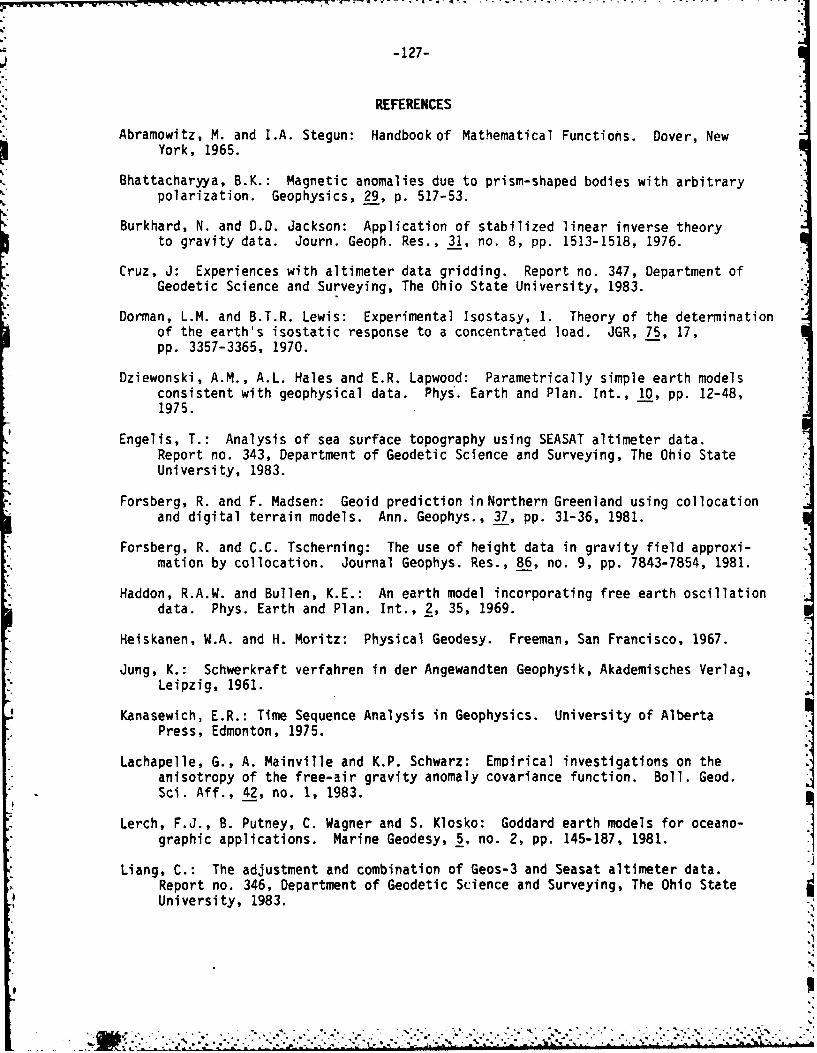
W'U . ' L W r '%T , . i . . :- . r rrr-7r-r y '. , o . < .-.. .- . . '" - -'

-127-

REFERENCES

Abramowitz, M. and I.A. Stegun: Handbook of Mathematical Functions. Dover, NewYork, 1965.

Bhattacharyya, B.K.: Magnetic anomalies due to prism-shaped bodies with arbitrarypolarization. Geophysics, 29, p. 517-53.

Burkhard, N. and D.D. Jackson: Application of stabilized linear inverse theoryto gravity data. Journ. Geoph. Res., 31, no. 8, pp. 1513-1518, 1976.

Cruz, J: Experiences with altimeter data gridding. Report no. 347, Department ofGeodetic Science and Surveying, The Ohio State University, 1983.

Dorman, L.M. and B.T.R. Lewis: Experimental Isostasy, 1. Theory of the determinationof the earth's isostatic response to a concentrated load. JGR, 75, 17,pp. 3357-3365, 1970.

Dziewonski, A.M., A.L. Hales and E.R. Lapwood: Parametrically simple earth modelsconsistent with geophysical data. Phys. Earth and Plan. Int., 10, pp. 12-48,1975.

Engelis, T.: Analysis of sea surface topography using SEASAT altimeter data.Report no. 343, Department of Geodetic Science and Surveying, The Ohio StateUniversity, 1983.

Forsberg, R. and F. Madsen: Geoid prediction in Northern Greenland using collocationand digital terrain models. Ann. Geophys., 37, pp. 31-36, 1981.

Forsberg, R. and C.C. Tscherning: The use of height data in gravity field approxi-mation by collocation. Journal Geophys. Res., 86, no. 9, pp. 7843-7854, 1981.

Haddon, R.A.W. and Bullen, K.E.: An earth model incorporating free earth oscillation

data. Phys. Earth and Plan. Int., 2, 35, 1969.

Heiskanen, W.A. and H. Moritz: Physical Geodesy. Freeman, San Francisco, 1967.

Jung, K.: Schwerkraft verfahren in der Angewandten Geophysik, Akademisches Verlag,Leipzig, 1961.

Kanasewich, E.R.: Time Sequence Analysis in Geophysics. University of AlbertaPress, Edmonton, 1975.

Lachapelle, G., A. Mainville and K.P. Schwarz: Empirical investigations on theanisotropy of the free-air gravity anomaly covariance function. Boll. Geod.Sci. Aff., 42, no. 1, 1983.

Lerch, F.J., B. Putney, C. Wagner and S. Klosko: Goddard earth models for oceano-graphic applications. Marine Geodesy, 5, no. 2, pp. 145-187, 1981.

Liang, C.: The adjustment and combination of Geos-3 and Seasat altimeter data.

Report no. 346, Department of Geodetic Science and Surveying, The Ohio StateUniversity, 1983.

.......................................... . 7

.m. . . k . .- * .r7w- . -. ,.-. .. C. . r - i • m ° m -r-, - C- r r C- C C . r .

-128-

MacMillan, W.D.: Theoretical Mechanics, vol. 2, The theory of the potential.Dover, New York, 1958.

Moritz, H.: Linear solutions of the geodetic boundary value problem. Reportno. 79, Department of Geodetic Science and Surveying, The Ohio State University,1966.

Moritz, H.: On the use of the terrain correction in solving Molodensky's problem.Department of Geodetic Science, Riport no. 108, The Ohio State University,1968a.

Moritz, H.: Density distributions for the equipotential ellipsoid. Department ofGeodetic Science, Report no. 115, The Ohio State University, 1968b.

Moritz, H.: Least squares collocation as a gravitational inverse problem. Departmentof Geodetic Science and Surveying, Report no. 249, The Ohio State University,1976.

Moritz, H.: Advanced physical geodesy. Herbert Wichmann Verlag, Karlsruhe, 1980.

Nash, R.A. and S.K. Jordan: Statistical geodesy - an engineering perspective.Proc. IEEE, 66, no. 5, pp. 532-550, 1978.

Papoulis, A.: Systems and transformations with applications in optics. McGraw-Hill,New York, 1968.

Pedersen, L.B.: Constrained inversion of potential field data. Geoph. Prosp.,27, pp. 726-748, 1979.

Rapp, R.H.: The earth's gravity field to degree and order 180 using SEASAT altimeterdata, terrestrial gravity data, and other data. Reports of the Departmentof Geodetic Science and Surveying, no. 322, The Ohio State University, 1981.

Rapp, R.H.: Degree variances of the earth's potential, topography and its isostaticcompensation. Bull. Geod. 56, pp. 84-94, 1982.

Rapp, R.H.: Problems in the development of improved high degree spherical harmonicexpansions of the gravity field. Paper presented at the workshop "Gravity fieldmodelling on a local basis", The Ohio State University, October 1983.

Rummel, R., K.-P. Schwarz and M. Gerstl: Least squares collocation and regular-ization. Bull. geod., 53, pp. 343-361, 1979.

Sanso, F. and C.C. Tscherning: Mixed collocation, a proposal. QuaternionesGeodaesiae, 3, no. 1, 1982.

Sideris, M.G.: Computation of terrain corrections using the fast fourier transform.IAG SSG 4.91 handout, January 1984.

SUnkel, H.; The estimation of free-air anomalies. Reports of the Department ofGeodetic science and Surveying, Report no. 315, The Ohio State University,1981a.

-129-

SUnkel, H.: Point mass models and the anomalous gravity field. Reports of theDepartment of Geodetic Science and Surveying, Report no. 328, The Ohio StateUniversity, 1981b.

Tscherning, C.C.: Some simple methods for the unique assignment of a densitydistribution to a harmonic fanction. Reports of the Department of GeodeticScience and Surveying, Report no. 213, The Ohio State University, 1974.

Tscherning, C.C. and R. Forsberg: Prediction test using least squares collocationand residual terrain reduction. In K.-P. Schwarz (ed.): Techniques to predictgravity anomalies and deflections of the vertical in mountaineous areas,Department of Surveying Engineering, report 30004, University of Calgary,Alberta, 1983.

Tscherning, C.C.: A brief introduction to geoid modelling using collocation withsome results from Scandanavia and Greenland. Preprint, submitted to MarineGeodesy, 1983.

/.

,S