Aprendizajereforzado Mannen
91
LEARNING TO PLAY CHESS USING REINFORCEMENT LEARNING WITH DATABASE GAMES Henk Mannen supervisor: dr. Marco Wiering MASTER’S THESIS COGNITIVE ARTIFICIAL INTELLIGENCE UTRECHT UNIVERSITY OCTOBER 2003
Transcript of Aprendizajereforzado Mannen

7/27/2019 Aprendizajereforzado Mannen
http://slidepdf.com/reader/full/aprendizajereforzado-mannen 1/91
LEARNING TO PLAY CHESS USING
REINFORCEMENT LEARNING WITH
DATABASE GAMES
Henk Mannensupervisor: dr. Marco Wiering
MASTER’S THESIS COGNITIVE ARTIFICIAL INTELLIGENCE
UTRECHT UNIVERSITY
OCTOBER 2003

7/27/2019 Aprendizajereforzado Mannen
http://slidepdf.com/reader/full/aprendizajereforzado-mannen 2/91
”Of chess it has been said that life is not long enough for
it, but that is the fault of life, not chess.” - Irving Chernev
ii
7/27/2019 Aprendizajereforzado Mannen
http://slidepdf.com/reader/full/aprendizajereforzado-mannen 3/91
Table of Contents
Table of Contents iii
List of Tables vi
List of Figures viii
Abstract xi
Acknowledgements xiii
1 Introduction 1
1.1 Chess and Artificial Intelligence . . . . . . . . . . . . . . 11.2 Machine learning . . . . . . . . . . . . . . . . . . . . . . 31.3 Game-playing . . . . . . . . . . . . . . . . . . . . . . . . 31.4 Learning chess programs . . . . . . . . . . . . . . . . . . 41.5 Relevance for Cognitive Artificial Intelligence . . . . . . . 71.6 Outline of this thesis . . . . . . . . . . . . . . . . . . . . 8
2 Machine learning 112.1 Introduction . . . . . . . . . . . . . . . . . . . . . . . . . 112.2 Supervised learning . . . . . . . . . . . . . . . . . . . . . 11
2.3 Unsupervised learning . . . . . . . . . . . . . . . . . . . 122.4 Reinforcement learning . . . . . . . . . . . . . . . . . . . 122.5 Markov decision processes . . . . . . . . . . . . . . . . . 132.6 Reinforcement learning vs. classical algorithms . . . . . . 142.7 Online and offline reinforcement learning . . . . . . . . . 152.8 Q-learning . . . . . . . . . . . . . . . . . . . . . . . . . . 152.9 TD-learning . . . . . . . . . . . . . . . . . . . . . . . . . 16
iii

7/27/2019 Aprendizajereforzado Mannen
http://slidepdf.com/reader/full/aprendizajereforzado-mannen 4/91
2.10 TD(λ)-learning . . . . . . . . . . . . . . . . . . . . . . . 172.11 TDLeaf-learning . . . . . . . . . . . . . . . . . . . . . . . 182.12 Reinforcement learning to play games . . . . . . . . . . . 19
3 Neural networks 213.1 Multi-layer perceptron . . . . . . . . . . . . . . . . . . . 213.2 Activation functions . . . . . . . . . . . . . . . . . . . . 223.3 Training the weights . . . . . . . . . . . . . . . . . . . . 233.4 Forward pass . . . . . . . . . . . . . . . . . . . . . . . . 243.5 Backward pass . . . . . . . . . . . . . . . . . . . . . . . 253.6 Learning rate . . . . . . . . . . . . . . . . . . . . . . . . 26
4 Learning to play Tic-Tac-Toe 294.1 Why Tic-Tac-Toe? . . . . . . . . . . . . . . . . . . . . . 294.2 Rules of the game . . . . . . . . . . . . . . . . . . . . . . 294.3 Architecture . . . . . . . . . . . . . . . . . . . . . . . . . 304.4 Experiment . . . . . . . . . . . . . . . . . . . . . . . . . 314.5 Testing . . . . . . . . . . . . . . . . . . . . . . . . . . . . 324.6 Conclusion . . . . . . . . . . . . . . . . . . . . . . . . . . 34
5 Chess programming 37
5.1 The evaluation function . . . . . . . . . . . . . . . . . . 375.2 Human vs. computer . . . . . . . . . . . . . . . . . . . . 385.3 Chess features . . . . . . . . . . . . . . . . . . . . . . . . 395.4 Material balance . . . . . . . . . . . . . . . . . . . . . . 425.5 Mobility . . . . . . . . . . . . . . . . . . . . . . . . . . . 435.6 Board control . . . . . . . . . . . . . . . . . . . . . . . . 435.7 Connectivity . . . . . . . . . . . . . . . . . . . . . . . . . 445.8 Game tree search . . . . . . . . . . . . . . . . . . . . . . 445.9 MiniMax . . . . . . . . . . . . . . . . . . . . . . . . . . . 455.10 Alpha-Beta search . . . . . . . . . . . . . . . . . . . . . 455.11 Move ordering . . . . . . . . . . . . . . . . . . . . . . . . 475.12 Transposition table . . . . . . . . . . . . . . . . . . . . . 485.13 Iterative deepening . . . . . . . . . . . . . . . . . . . . . 485.14 Null-move pruning . . . . . . . . . . . . . . . . . . . . . 485.15 Quiescence search . . . . . . . . . . . . . . . . . . . . . . 495.16 Opponent-model search . . . . . . . . . . . . . . . . . . . 49
iv

7/27/2019 Aprendizajereforzado Mannen
http://slidepdf.com/reader/full/aprendizajereforzado-mannen 5/91
6 Learning to play chess 516.1 Setup experiments . . . . . . . . . . . . . . . . . . . . . 516.2 First experiment: piece values . . . . . . . . . . . . . . . 526.3 Second experiment: playing chess . . . . . . . . . . . . . 55
7 Conclusions and suggestions 617.1 Conclusions . . . . . . . . . . . . . . . . . . . . . . . . . 617.2 Further work . . . . . . . . . . . . . . . . . . . . . . . . 62
A Derivation of the back-propagation algorithm 63
B Chess features 67
Bibliography 74
v

7/27/2019 Aprendizajereforzado Mannen
http://slidepdf.com/reader/full/aprendizajereforzado-mannen 6/91
vi

7/27/2019 Aprendizajereforzado Mannen
http://slidepdf.com/reader/full/aprendizajereforzado-mannen 7/91
List of Tables
4.1 Parameters of the Tic-Tac-Toe networks . . . . . . . . . 33
6.1 Parameters of the chess networks . . . . . . . . . . . . . 51
6.2 Material values . . . . . . . . . . . . . . . . . . . . . . . 52
6.3 Program description . . . . . . . . . . . . . . . . . . . . 57
6.4 Features of tscp 1.81 . . . . . . . . . . . . . . . . . . . . 57
6.5 Tournament crosstable . . . . . . . . . . . . . . . . . . . 58
6.6 Performance . . . . . . . . . . . . . . . . . . . . . . . . . 58
vii

7/27/2019 Aprendizajereforzado Mannen
http://slidepdf.com/reader/full/aprendizajereforzado-mannen 8/91
viii

7/27/2019 Aprendizajereforzado Mannen
http://slidepdf.com/reader/full/aprendizajereforzado-mannen 9/91
List of Figures
2.1 Principal variation tree . . . . . . . . . . . . . . . . . . . 19
3.1 A multi-layer perceptron . . . . . . . . . . . . . . . . . . 22
3.2 Sigmoid and stepwise activation functions . . . . . . . . 24
3.3 Gradient descent with small η . . . . . . . . . . . . . . . 26
3.4 Gradient descent with large η . . . . . . . . . . . . . . . 27
4.1 Hidden layer of 40 nodes for Tic-Tac-Toe . . . . . . . . . 34
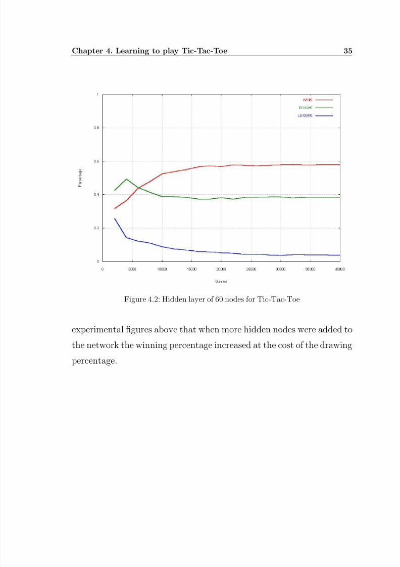
4.2 Hidden layer of 60 nodes for Tic-Tac-Toe . . . . . . . . . 35
4.3 Hidden layer of 80 nodes for Tic-Tac-Toe . . . . . . . . . 36
5.1 Example chess position . . . . . . . . . . . . . . . . . . . 39
5.2 MiniMax search tree . . . . . . . . . . . . . . . . . . . . 46
5.3 MiniMax search tree with alpha-beta cutoffs . . . . . . . 47
6.1 Hidden layer of 40 nodes for piece values . . . . . . . . . 54
6.2 Hidden layer of 60 nodes for piece values . . . . . . . . . 55
6.3 Hidden layer of 80 nodes for piece values . . . . . . . . . 56
B.1 Isolated pawn on d4 . . . . . . . . . . . . . . . . . . . . 68
ix

7/27/2019 Aprendizajereforzado Mannen
http://slidepdf.com/reader/full/aprendizajereforzado-mannen 10/91
B.2 Doubled pawns . . . . . . . . . . . . . . . . . . . . . . . 69
B.3 Passed pawns on f5 and g5 . . . . . . . . . . . . . . . . . 69B.4 Pawn fork . . . . . . . . . . . . . . . . . . . . . . . . . . 70
B.5 Knight fork . . . . . . . . . . . . . . . . . . . . . . . . . 70
B.6 Rooks on the seventh rank . . . . . . . . . . . . . . . . . 71
B.7 Board control . . . . . . . . . . . . . . . . . . . . . . . . 72
B.8 Connectivity . . . . . . . . . . . . . . . . . . . . . . . . . 72
x
7/27/2019 Aprendizajereforzado Mannen
http://slidepdf.com/reader/full/aprendizajereforzado-mannen 11/91
Abstract
In this thesis we present some experiments in the training of different
evaluation functions for a chess program through reinforcement learn-
ing. A neural network is used as the evaluation function of the chess
program. Learning occurs by using TD( λ)-learning on the results of
high-level database games. The main experiment shows that separated
networks for different game situations lead to the best result.
keywords : Reinforcement learning, Temporal difference learning,
Neural Networks, Game Playing, Chess, Database games
xi

7/27/2019 Aprendizajereforzado Mannen
http://slidepdf.com/reader/full/aprendizajereforzado-mannen 12/91

7/27/2019 Aprendizajereforzado Mannen
http://slidepdf.com/reader/full/aprendizajereforzado-mannen 13/91
Acknowledgements
I would like to thank dr. Marco Wiering, my supervisor, for his many
suggestions and constant support during this research. I am also thank-
ful to Jan Peter Patist for the fruitful discussions we had.
Of course, I am also grateful to my girlfriend Lisette, my parents and
sister for their patience and love.
A special word of thanks goes to Tom Kerrigan for his guidance inthe world of chess programming.
Finally, I wish to thank my computer for doing all the hard work.
Utrecht, the Netherlands Henk Mannen
July 4, 2003
xiii

7/27/2019 Aprendizajereforzado Mannen
http://slidepdf.com/reader/full/aprendizajereforzado-mannen 14/91
Chapter 1
Introduction
1.1 Chess and Artificial Intelligence
Playing a good game of chess is often associated with intelligent be-
haviour. Therefore chess has always been a challenging problem domain
for artificial intelligence(AI) research. In 1965 the Russian mathemati-
cian Alexander Kronrod put it nicely: ”Chess is the Drosophila of AI”.The first chess machine was already built in 1769 by the Hungarian no-
bleman and engineer Wolfgang van Kempelen[Michael, 1975]. His chess
playing automaton, which was later called The Turk , was controlled by
a chessmaster who was hidden inside the machine. It took about ten
years for the public to discover this secret. In a way Van Kempelen
anticipated on the Turing test: a device is intelligent if it can pass for
a human in a written question-and-answer session [Turing, 1950].
In the 1950s, Claude Shannon and Alan Turing offered ideas for design-
ing chess programs [Shannon, 1950, Turing, 1999]. The first working
chess playing program, called TurboChamp, was written by Alan Turing
1

7/27/2019 Aprendizajereforzado Mannen
http://slidepdf.com/reader/full/aprendizajereforzado-mannen 15/91
2 Chapter 1. Introduction
in 1951. It was never run on a computer, instead it was tested by hand
against a mediocre human player, and lost. Less than half a century of chess programming later, a chess program defeated the world champion.
Gary Kasparov was beaten in 1997 by the computer program Deep
Blue in a match over six games by 3,5-2,5[Schaeffer and Plaat, 1991].
Despite this breakthrough, world class human players are still consid-
ered playing better chess than computer programs. The game is said
to be too complex to be completely understood by humans, but also
too complex to be computed by the most powerful computer. It is
impossible to evaluate all possible board positions. In a game of 40
moves, the number of possible chess games has been estimated at 10120
[Shannon, 1950]. This is because there are many different ways of going
through the various positions. The amount of different board positions
is about 1043 [Shannon, 1950]. Most of the 1043 possible positions are
very unbalanced, with one side clearly winning. To solve chess one only
requires knowing the value of about 1020 critical positions. In reference,
1075 atoms are thought to exist in the entire universe. This indicates
the complexity of the game of chess. Nevertheless, researchers in the
field of artificial intelligence keep on trying to invent new ways to tackle
this problem domain, in order to test their intelligent algorithms.

7/27/2019 Aprendizajereforzado Mannen
http://slidepdf.com/reader/full/aprendizajereforzado-mannen 16/91
Chapter 1. Introduction 3
1.2 Machine learning
Machine learning is the branch of artificial intelligence which studies
learning methods for creating intelligent systems. These systems are
trained with the use of a learning algorithm for a domain specific prob-
lem or task. One of these machine learning methods is reinforcement
learning. An agent can learn to behave in a certain way by receiving
punishment or reward on its chosen actions.
1.3 Game-playing
Game-playing is a very popular machine learning research domain for
AI. This is due the fact that board games offer a fixed environment, easy
measurement of taken actions(result of the game) and enough complex-
ity. A human expert and a game-playing program have quite different
search procedures. A human expert makes use of a vast amount of do-
main specific knowledge. Such knowledge allows the human expert to
analyze a few moves for each game situation, without wasting time an-
alyzing irrelevant moves. On the contrary, the game-playing program
uses ’brute-force’ searches. It explores as many alternative moves and
consequences as possible.A lot of game-learning programs have been developed in the past decades.
Samuel’s checkers program [Samuel, 1959, Samuel, 1967] and Tesauro’s
TD-Gammon[Tesauro, 1995] were important breakthroughs. Samuel’s
checkers program was the first successful checkers learning program

7/27/2019 Aprendizajereforzado Mannen
http://slidepdf.com/reader/full/aprendizajereforzado-mannen 17/91
4 Chapter 1. Introduction
which was able to defeat amateur players. He used a search procedure
which was suggested by Shannon in 1950, called MiniMax
[Shannon, 1950](see section 5.9). Samuel used two different types of
learning: generalization and rote learning.
With generalization all board positions are evaluated by one polyno-
mial function.
With rote learning board positions are memorized with their score at
search ends. Recomputing the value, if such a position occurs again,then isn’t necessary anymore. This saves computing time and therefore
makes it possible to search deeper in the search tree.
In 1995 Gerald Tesauro presented a game-learning program, called
TD-Gammon[Tesauro, 1995]. The program was able to compete with
the world’s strongest backgammon players. It was trained by playing
against itself and learning on the outcome of those games. It scored
board positions by using a neural network(NN) as its evaluation func-
tion. Tesauro made use of temporal difference learning(TD-learning ,
see section 2.9), a method which was in concept the same as Samuel’s
learning method.
1.4 Learning chess programs
In 1993 Michael Gherrity introduced his general learning system, called
Search And Learning (SAL)[Gherrity, 1993]. SAL can learn any two-
player board game that can be played on a rectangular board and uses

7/27/2019 Aprendizajereforzado Mannen
http://slidepdf.com/reader/full/aprendizajereforzado-mannen 18/91
Chapter 1. Introduction 5
fixed types of pieces. SAL is trained after every game it plays by using
temporal difference learning. Chess, Tic-Tac-Toe were the games SAL
was tested on. SAL achieved good results in Tic-Tac-Toe and connect
four, but the level of play it achieved in chess, with a search-depth of 2
ply, was poor.
Morph[Gould and Levinson, 1991, Levinson, 1995] is also a learning
chess program like SAL, with the difference that Morph only plays
chess. SAL and Morph also have two other distinguishing similaritiesbetween them in their design. They contain a set of search methods as
well as evaluation functions.
The search methods take the database that is in front of them and
decide an appropriate next move.
Evaluation functions assign weights to given patterns and evaluate them
for submission to the database for future use. Morph represents chess
knowledge as weighted patterns(pattern-weight pairs ). The patterns
are graphs of attack and defense relationships between pieces on the
board and vectors of relative material difference between the players.
For each position, it computes which patterns match the position and
uses a global formula to combine the weights of the matching patterns
into an evaluation. Morph plays the move with the best evaluation,
using a search-depth of 1 ply. Due to this low search-depth Morphoften loses material or overlooks a mate.
Its successor, MorphII[Levinson, 1994], is also capable of playing other
games besides chess. Morph II solved some of Morph’s weaknesses

7/27/2019 Aprendizajereforzado Mannen
http://slidepdf.com/reader/full/aprendizajereforzado-mannen 19/91
6 Chapter 1. Introduction
which resulted in a better level of play in chess.
MorphIII and MorphIV are further expansions of Morph II, primarily
focusing on chess. However, the level of play reached still can’t be called
satisfactory. This is partly due the fact that it uses such a low search-
depth. Allowing deeper searches slows down the system enormously.
Another learning chess program is Sebastian Thrun’s NeuroChess
[Thrun, 1995]. NeuroChess has two neural networks, V and M . V
is the evaluation function, which gives an output value for the inputvector of 175 hand-written chess features. M is a neural network which
predicts the value of an input vector two ply later. M is an explanation-
based neural network (EBNN)[Mitchell and Thrun, 1993], which is the
central learning mechanism of NeuroChess. The EBNN is used for
training the evaluation function V . This EBNN is trained on 120,000
grand-master database games. V learns from each position in each
game, using TD-learning to compute a target evaluation value and M
to compute a target slope of the evaluation function. V is trained on
120,000 grand-master games and 2,400 self-play games. Neurochess
uses the framework of the chess program GnuChess. The evaluation
function of GnuChess was replaced by the trained neural network V .
NeuroChess defeated GnuChess in about 13% of the games. A version
of NeuroChess which did not use the chess model EBNN, won in about10% of the games. GnuChess and NeuroChess both were set to a search-
depth of 3 ply.
Jonathan Baxter developed KnightCap[Baxter et al., 1997]

7/27/2019 Aprendizajereforzado Mannen
http://slidepdf.com/reader/full/aprendizajereforzado-mannen 20/91
Chapter 1. Introduction 7
which is a strong learning chess program. It uses TDLeaf-learning (see
section 2.11), which is an enhancement of Richard Sutton’s TD(λ)-
learning [Sutton, 1988](see section 2.10). KnightCap makes use of a
linear evaluation function. KnightCap learns from the games it plays.
The modifications in the evaluation function of KnightCap are based
upon the outcome of its games. It also uses a book learning algorithm
which enables it to learn opening lines and endgames.
1.5 Relevance for Cognitive Artificial Intelligence
Cognitive Artificial Intelligence(CKI in Dutch) focuses on the possibil-
ities to design systems which show intelligent behavior. Behavior which
we will address to as being intelligent when shown by human beings.
Cognitive stems from the Latin word Cogito, i.e., the ability to think.
It is not about attempting to exactly copy a human brain and its func-
tionality. Moreover, it is about mimicking its output.
Playing a good game of chess is generally associated with showing in-
telligent behavior. Above all, the evaluation function, which assigns a
certain evaluation score to a certain board position, is the measuring
rod for intelligent behavior in chess. A bad position should receive arelatively low score and a good position a relatively high score. This
assignment work is done by both humans and computers and can be
seen as the output of their brain. Therefore, a chess program with
proper output can be called (artificial) intelligent.
7/27/2019 Aprendizajereforzado Mannen
http://slidepdf.com/reader/full/aprendizajereforzado-mannen 21/91
8 Chapter 1. Introduction
Another qualification for an agent to be called intelligent is its abil-
ity to learn something. An agent’s behavior can be adapted by using
machine learning techniques. By learning on the outcome of example
chess games we have a means of improving the agent’s level of play.
In this thesis we attempt to create a reasonable nonlinear evaluation
function of a chess program through reinforcement learning on database
examples1. The program evaluates a chess position by using a neural
network as its evaluation function. Learning is accomplished by usingreinforcement learning on chess positions which occur in a database of
tournament games. We are interested in the program’s level of play
that can be reached in a short amount of time. We will compare eight
different evaluation functions by playing a round robin tournament.
1.6 Outline of this thesis
We will now give a brief overview of the upcoming chapters.
The next chapter discusses some machine learning methods which can
be used.
Chapter three is about neural networks and their techniques.
Chapter four is on learning a neural network to play the game of Tic-
Tac-Toe. This experiment basically will give us insight in the ability of
a neural network to generalize on a lot of different input patterns.
Chapter five discusses some general issues of chess programming.
1we used a PentiumII 450mhz and coded in C++.

7/27/2019 Aprendizajereforzado Mannen
http://slidepdf.com/reader/full/aprendizajereforzado-mannen 22/91
Chapter 1. Introduction 9
Chapter six shows the experimental results of training several neural
networks on the game of chess.
Chapter seven concludes and also several suggestions for future work
will be put forward.

7/27/2019 Aprendizajereforzado Mannen
http://slidepdf.com/reader/full/aprendizajereforzado-mannen 23/91

7/27/2019 Aprendizajereforzado Mannen
http://slidepdf.com/reader/full/aprendizajereforzado-mannen 24/91
Chapter 2
Machine learning
2.1 Introduction
In order to make our chess agent intelligent, we would like it to learn
from the input we feed it. We can use several learning methods to reach
this goal. The learning algorithms can be divided into three groups:
supervised learning, unsupervised learning and reinforcement learning.
2.2 Supervised learning
Supervised learning occurs when a neural network is trained by giving
it examples of the task we want it to learn, i.e., learning with a teacher.
The way this is done is by providing a set of pairs of patterns wherethe first pattern of each pair is an example of an input pattern and the
second pattern is the output pattern that the network should produce
for that input. The discrepancies in the output between the actual
output and the desired output are used to determine the changes in
11
7/27/2019 Aprendizajereforzado Mannen
http://slidepdf.com/reader/full/aprendizajereforzado-mannen 25/91
12 Chapter 2. Machine learning
the weights of the network.
2.3 Unsupervised learning
With unsupervised learning there is no target output given by an ex-
ternal supervisor. The learning takes place in a self-organizing manner.
Generally speaking, unsupervised learning algorithms attempt to ex-
tract common sets of features present in the input data. An advantage
of these learning algorithms is their ability to correctly cluster input
patterns with missing or erroneous data. The system can use the ex-
tracted features it has learned from the training data, to reconstruct
structured patterns from corrupted input data. This invariance of the
system to noise, allows for more robust processing in performing recog-
nition tasks.
2.4 Reinforcement learning
With reinforcement learning algorithms an agent can improve its per-
formance by using the feedback it gets from the environment. Thisenvironmental feedback is called the reward signal . With reinforcement
learning the program receives feedback, as is the same with supervised
learning.
Reinforcement learning differs from supervised learning in the way how

7/27/2019 Aprendizajereforzado Mannen
http://slidepdf.com/reader/full/aprendizajereforzado-mannen 26/91
Chapter 2. Machine learning 13
an error in the output is treated. With supervised learning the feed-
back information is what exact output was needed. The feedback with
reinforcement learning only contains information on how good the ac-
tual output was. By trial-and-error the agent learns to act in order to
receive maximum reward.
Important is the trade-off between exploitation and exploration. On
the one hand, the system should chose actions which lead to the high-
est reward, based upon previous encounters. On the other hand italso should try new actions which could possibly lead to even higher
rewards.
2.5 Markov decision processes
Let us take a look on the decision processes of our chess agent. With
chess the result of a game can be either a win, a loss or a draw. Our
agent must make a sequence of decisions which will result in one of those
final outcomes of the game, which is known as a sequential decision
problem. This is a lot more difficult than single decision problems,
where the result of a taken action is immediately apparent.
The problem of calculating an optimal policy in an accessible, stochasticenvironment with a known transition model is called a Markov decision
problem (MDP). A policy is a function, which assigns a choice of action
to each possible history of states and actions. The Markov property
holds if the transition probabilities from any given state depend only
7/27/2019 Aprendizajereforzado Mannen
http://slidepdf.com/reader/full/aprendizajereforzado-mannen 27/91
14 Chapter 2. Machine learning
on the state and not on the previous history. In a Markov decision
process, the agent selects its best action based on its current state.
2.6 Reinforcement learning vs. classical algorithms
Reinforcement Learning is a technique for solving Markov Decision
Problems. Classical algorithms for calculating an optimal policy, such
as value iteration and policy iteration[Bellman, 1961], can only be used
if the amount of possible states is small and the environment is not too
complex. This is because transition probabilities have to be calculated.
These calculations need to be stored and can lead to a storage problem
with large state spaces.
Reinforcement learning is capable of solving these Markov decision
problems because no calculation or storage of the transition proba-
bilities is needed. With large state spaces, it can be combined with a
function approximator such as a neural network, to approximate theevaluation function.
There are a lot of different reinforcement learning algorithms. Below
we will discuss two important algorithms, Q-learning
[Watkins and Dayan, 1992] and TD-learning [Sutton, 1988].

7/27/2019 Aprendizajereforzado Mannen
http://slidepdf.com/reader/full/aprendizajereforzado-mannen 28/91
Chapter 2. Machine learning 15
2.7 Online and offline reinforcement learning
We can chose between learning after each visited state, i.e., online learn-
ing , or wait until a goal is reached and then update the parameters, i.e.,
offline learning or batch learning . Online learning has two uncertainties
[Ben-David et al., 1995]:
1. what is the target function which is consistent with the data
2. what patterns will be encountered in the future
Offline learning also suffers from the first uncertainty described above.
The second uncertainty only goes for online learning because with of-
fline learning the sequence of patterns is known.
We used offline learning in our experiments, thus updating the evalua-
tion function after the sequence of board positions of a database-game
is known.
2.8 Q-learning
Q-learning is a reinforcement learning algorithm that does not need a
model of its environment and can be used online. Q-learning algorithms
work by estimating the values of state-action pairs. The value Q(s, a) isdefined to be the expected discounted sum of future payoffs obtained by
taking action a from state s and following the current optimal policy
thereafter. Once these values have been learned, the optimal action
from any state is the one with the highest Q-value.

7/27/2019 Aprendizajereforzado Mannen
http://slidepdf.com/reader/full/aprendizajereforzado-mannen 29/91
16 Chapter 2. Machine learning
The values for the state-action pairs are learnt by the following Q-
learning rule[Watkins, 1989]:
Q(s, a) = (1 − α) ·Q(s, a) + α · (r(s) + γ · maxa
Q(s, a)) (2.8.1)
where:
• α is the learning rate
• s is the current state
• a is the chosen action for the current state
• s is the next state
• a is the best possible action for the next state
• r(s) is the received scalar reward
• γ is the discount factor
The discount factor γ is used to prefer immediate rewards over de-
layed rewards.
2.9 TD-learning
TD-learning is a reinforcement learning algorithm that assigns utility
values to states alone instead of state-action pairs. The desired values
of the states are updated by the following function [Sutton, 1988]:
V (st) = V (st) + α · (rt + γ · V (st+1) − V (st)) (2.9.1)
7/27/2019 Aprendizajereforzado Mannen
http://slidepdf.com/reader/full/aprendizajereforzado-mannen 30/91
Chapter 2. Machine learning 17
where:
• α is the learning rate
• rt is the received scalar reward of state t
• γ is the discount factor
• V (st) is the value of state t
• V (st+1) is value of the next state
• V (st) is the desired value of state t
2.10 TD(λ)-learning
TD(λ)-learning is a reinforcement learning algorithm which takes into
account the result of a stochastic process and the prediction of the
result by the next state. The desired value of the terminal state stend is
for a board game:
V (stend) = gameresult (2.10.1)
The desired values of the other states are given by the following func-
tion:
V (st) = λ · V (st+1) + α · ((1− λ) · (rt + γ · V (st+1)− V (st))) (2.10.2)
where:
• rt is the received scalar reward of state t

7/27/2019 Aprendizajereforzado Mannen
http://slidepdf.com/reader/full/aprendizajereforzado-mannen 31/91
18 Chapter 2. Machine learning
• γ is the discount factor
• V (st) is the value of state t
• V (st+1) is the value of the next state
• V (st) is the desired value of state t
• V (st+1) is the desired value of state t+ 1
• 0≤ λ ≤1 controls the feedback of the desired value of future states
If λ is 1, the desired value for all states will be the same as the
desired value for the terminal state. If λ is 0, the desired value of a
state will receives no feedback of the desired value of the next state.
With λ set to 0, formula 2.10.2 is the same as formula 2.9.1. Therefore
normal TD-learning is also called TD(0)-learning .
2.11 TDLeaf-learning
TDLeaf-learning[Beal, 1997] is a reinforcement learning algorithm which
combines TD(λ)-learning with game tree search. It makes use of the
leaf node of the principal variation. The principle variation is the al-ternation of best own moves and best opponent moves from the root to
the depth of the tree. The score of the leaf node of the principal vari-
ation is assigned to the root node. A principal variation tree is shown
in figure 2.1.

7/27/2019 Aprendizajereforzado Mannen
http://slidepdf.com/reader/full/aprendizajereforzado-mannen 32/91
Chapter 2. Machine learning 19
Figure 2.1: Principal variation tree
2.12 Reinforcement learning to play games
In our experiments we used the TD(λ)-learning algorithm to learn from
the occurred board positions in a game. In order to learn an evaluation
function for the game of chess we made use of a database which contains
games played by human experts. The games are stored in the file format
Portable Game Notation (PGN). We wrote a program which converts a
game in PGN format to board positions.
A board position is propagated forward through a neural network(see
section 3.3), with the output being the value of the position. The error
between the value and the desired value of a board position is called
the TD-error :
TD-error = V (st) − V (st) (2.12.1)
This error is used to change the weights of the neural network during
the backward pass (see section 3.4).
We will repeat this learning process on a huge amount of database

7/27/2019 Aprendizajereforzado Mannen
http://slidepdf.com/reader/full/aprendizajereforzado-mannen 33/91
20 Chapter 2. Machine learning
games. It’s also possible to learn by letting the program play against
itself. Learning on database examples has two advantages over learning
from self-play.
Firstly, self-play is a much more time consuming learning method than
database training. With self-play a game first has to be played to
have training examples. With database training the games are already
played.
Secondly, with self-play it is hard to detect which moves are bad. If ablunder move is made by a player in a database game the other player
will mostly win the game. At the beginning of self-play a blunder will
often not be punished. This is because the program starts with ran-
domized weights and thus plays random moves. Lots of games therefore
are full of awkward looking moves and it is not easy to learn something
from those games.
However, self-play can be interesting to use after training the program
on database games. Since then a bad move will be more likely to get
punished, the program can learn from its own mistakes. Some bad
moves will never be played in a database game. The program may
prefer such a move above others which actually are better. With self-
play, the program will be able to play its preferred move and learn
from it. After training solely on database games, it could be possiblethat the program will favor a bad move just because it hasn’t had the
opportunity to find out why it is a bad move.

7/27/2019 Aprendizajereforzado Mannen
http://slidepdf.com/reader/full/aprendizajereforzado-mannen 34/91
Chapter 3
Neural networks
3.1 Multi-layer perceptron
A common used neural network architecture is the Multi-layer Per-
ceptron (MLP). A normal perceptron consists of an input layer and an
output layer. The MLP has an input layer, an output layer and one or
more hidden layers. Each node in a layer, other than the output layer,
has a connection with every node in the next layer. These connections
between nodes have a certain weight. Those weights can be updated by
back-propagating (see section 3.5) the error between the desired output
and actual output through the network.
The MLP is a feed-forward network, meaning that the connections be-
tween the nodes only fire from a lower layer to a higher layer, withthe input layer being the highest layer (see figure 3.1). The connection
pattern must not contain any cycles, thereby forming a directed acyclic
graph.
21

7/27/2019 Aprendizajereforzado Mannen
http://slidepdf.com/reader/full/aprendizajereforzado-mannen 35/91
22 Chapter 3. Neural networks
Figure 3.1: A multi-layer perceptron
3.2 Activation functions
When a hidden node receives its input it is necessary to use an ac-
tivation function on this input. In order to approximate a nonlinear
evaluation function, we need activation functions for the hidden nodes.
Without activation functions for the hidden nodes, the hidden nodes
would have linear input values and the MLP would have the same ca-
pabilities as a normal perceptron. This is because a linear function of
linear functions is still a linear function.
The power of multi-layer networks lies in their capability to represent
nonlinear functions. Provided that the activation function of the hid-
den layer nodes is nonlinear, an error back-propagation neural network
with an adequate number of hidden nodes is able to approximate everynon-linear function.
Activation functions with activation values between 1 and -1 can be
trained faster than functions with values between 0 and 1 because of
numerical conditioning. For hidden nodes, sigmoid activation functions

7/27/2019 Aprendizajereforzado Mannen
http://slidepdf.com/reader/full/aprendizajereforzado-mannen 36/91
Chapter 3. Neural networks 23
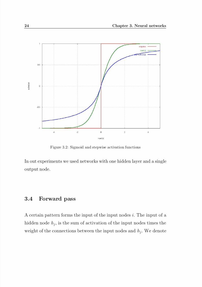
are preferable to threshold activation functions(see figure 3.2). A net-
work with threshold activation functions for its hidden nodes is difficult
to train. For back-propagation learning, the activation function must
be differentiable. The gradient of the stepwise activation function in
figure3.2 does not exist for x=0 and is 0 for 0<x<0.
We will use the activation function x/(1 + abs(x)) for the hidden nodes
in our experiments. It can be calculated faster than the tanh(x) acti-
vation function, which also has an activation value between -1 and 1.Faster calculation of the activation value makes it possible to evaluate
more positions in the same amount of time.
3.3 Training the weights
We want to train a multi-layer feed-forward network by gradient de-
scent to approximate an unknown function, based on some training
data consisting of pairs (x, t). The vector p represents a pattern of in-
put to the network, and the vector t the corresponding target(desired
output).
The training process of a neural network consists of 2 phases; the for-ward pass and the backward pass . The forward pass calculates the
output value for a certain input pattern. The backward pass starts
with the output layer and computes the local gradient for each node.
This gradient is used for updating the network’s weights.
7/27/2019 Aprendizajereforzado Mannen
http://slidepdf.com/reader/full/aprendizajereforzado-mannen 37/91
24 Chapter 3. Neural networks
Figure 3.2: Sigmoid and stepwise activation functions
In out experiments we used networks with one hidden layer and a single
output node.
3.4 Forward pass
A certain pattern forms the input of the input nodes i. The input of a
hidden node h j, is the sum of activation of the input nodes times the
weight of the connections between the input nodes and h j. We denote

7/27/2019 Aprendizajereforzado Mannen
http://slidepdf.com/reader/full/aprendizajereforzado-mannen 38/91
Chapter 3. Neural networks 25
the weight from node ii to node h j by wij.
h j =n
k=0
ii · wij (3.4.1)
After this an activation function g is used over the total sum of input
of a hidden node.
g(h j) =h j
1 + |h j|(3.4.2)
The input of the output node o is the sum of the activation of the
hidden nodes h times the weight of the connections between h and o.
We denote the weight from node h j to node o by w jo.
o =n
j=0
g(h j) · w jo (3.4.3)
3.5 Backward pass
The idea of the backward pass is to perform gradient descent on the
error considered as a function of the weights. This error is the deviation
in the target output value t and the actual output value o.
E = (t− o) (3.5.1)
The change in the weights of the connections between a hidden node
h j and the output node o is given by the following formula:
∆w jo = −η · E · g(h j) (3.5.2)
where η is the learning rate.

7/27/2019 Aprendizajereforzado Mannen
http://slidepdf.com/reader/full/aprendizajereforzado-mannen 39/91
26 Chapter 3. Neural networks
The change in the weights of the connections between an input node ii
and a hidden node h j is given by the following formula:
∆wij = −η · δ j · ii (3.5.3)
where δ j is given by:
δ j = E · w jo · g(h j) (3.5.4)
where w jo the weight from node h j to the output node o.
The derivation of the back-propagation algorithm is given in Appendix
A.
3.6 Learning rate
An important consideration is the learning rate η, which determines by
how much we change the weights w at each step. If η is too small, the
algorithm will take a long time to converge(see figure 3.3). On the other
Figure 3.3: Gradient descent with small η
hand, if η is too large, the weights w will be changed too radically(see
figure 3.4).

7/27/2019 Aprendizajereforzado Mannen
http://slidepdf.com/reader/full/aprendizajereforzado-mannen 40/91
Chapter 3. Neural networks 27
Figure 3.4: Gradient descent with large η

7/27/2019 Aprendizajereforzado Mannen
http://slidepdf.com/reader/full/aprendizajereforzado-mannen 41/91

7/27/2019 Aprendizajereforzado Mannen
http://slidepdf.com/reader/full/aprendizajereforzado-mannen 42/91
Chapter 4
Learning to play Tic-Tac-Toe
4.1 Why Tic-Tac-Toe?
The game of Tic-Tac-Toe is suitable to test if the designed neural net-
work could generalize well on the input given by the different board
positions because of the relatively small amount of possible board posi-
tions. Instead of starting directly with the game of chess it’s better tofocus on Tic-Tac-Toe first to detect any serious design- and program-
errors of the network. The game has the advantage to other board
games that it’s relatively easy to program and the result of a game is
yielded within 9 moves, which makes it little time-consuming to train
the network.
4.2 Rules of the game
The game of Tic-Tac-Toe is played by 2 players, each given a cross or
a circle as their playing material on a board of size 3 x 3, thus having
29
7/27/2019 Aprendizajereforzado Mannen
http://slidepdf.com/reader/full/aprendizajereforzado-mannen 43/91
30 Chapter 4. Learning to play Tic-Tac-Toe
nine empty squares at the beginning of the game. The player playing
with the cross starts the game, having the choice of occupying one of
the nine empty squares. After a move is made and the game is not yet
finished, the other player gets the turn.
A game is finished if a player wins or the board has no empty squares
left. The game ends in a win for a player when one has occupied three
neighbouring squares in a horizontal, vertical or diagonal way.
If there are no moves left the game ends in a draw. When the playersboth play the game optimally, a draw will be the result. Therefore the
game can be pretty dull when it is played by 2 players with a thorough
knowledge of it.
4.3 Architecture
The goal was to train a neural network which would function as an
evaluation function for a given board position. All possible moves are
evaluated with a search-depth of 1 half move(1 ply ). A possible move
leads to a new board position. The score for this position is yielded
by feeding the network with this board position as its input delivering
an output value. The network has an input layer, a hidden layer anda single output node. It is designed as a network with 10 input nodes,
representing the 9 squares of the Tic-Tac-Toe board and a node which
represents the player to move. The 9 input nodes responsible for the
squares can have three different values:

7/27/2019 Aprendizajereforzado Mannen
http://slidepdf.com/reader/full/aprendizajereforzado-mannen 44/91
Chapter 4. Learning to play Tic-Tac-Toe 31
• 1 for a cross occupying the square
• -1 for a circle occupying the square
• 0 for an empty square
Each node in the input-layer has a unique connection with each node
in the hidden layer.
We experimented with three different hidden layers, consisting of re-
spectively 80, 60 and 40 nodes. The nodes of the hidden layer each have
a connection with the single output node in the output-layer. When
the input of a node is known, the activation value can be calculated.
An activation function calculates the activation value for an input value.
The activation function was only applied to the nodes in the hidden
layer, not for the nodes of the input layer. For the node in the output
layer a linear activation function was used(i.e., the summed input).
4.4 Experiment
We implemented a win-block-random-player , which first checks if there
is an empty square on the board which will result in a direct win. If such
a square is present, the player will occupy the square to yield victory.If this is not the case it checks if there is an empty square on the board
which will lead to victory for his opponent[Boyan, 1992, Wiering, 1995].
If there is such a square, the player will occupy that square himself, thus
blocking a possible victory for his opponent.

7/27/2019 Aprendizajereforzado Mannen
http://slidepdf.com/reader/full/aprendizajereforzado-mannen 45/91
32 Chapter 4. Learning to play Tic-Tac-Toe
When none of the above cases are present the player will make a ran-
dom choice of the possible moves which are available in the current
position.
The player which uses the neural network as its evaluation function
checks the value the network delivers for the input pattern for every
available move. This input pattern is the resulting board position for
the selected move. It plays the move which yields the highest output
value in the neural network, thus having a search-depth of 1 ply.After a game is played, the training phase begins. Starting with the last
board position, being a win for cross(value=1) a win for square(value=-
1) or a draw(value=0). This input pattern is fed to the network, with
the value being the desired output. The desired output of the other
positions are calculated with the offline TD(λ)-learning method.
The network has random weights when the first game is played. The
evaluation of board positions in the beginning is therefore very inaccu-
rate. This gradually improves when more and more games are played
because the adaptation of the weights of the network. The robustness
of the evaluations grows over time.
4.5 Testing
The data obtained from each experiment were derived by averaging
each experiment over 10 runs. The parameters are given in table 4.1.
In the first experiment we used a network with a hidden layer of 40

7/27/2019 Aprendizajereforzado Mannen
http://slidepdf.com/reader/full/aprendizajereforzado-mannen 46/91
Chapter 4. Learning to play Tic-Tac-Toe 33
learning rate 0.01λ 0.9 → 0.02
input nodes 10hidden nodes 40/60/80output nodes 1
bias hidden nodes 1bias output node 0.25
Table 4.1: Parameters of the Tic-Tac-Toe networks
nodes(see figure 4.1). After 16,000 games the network was winningmore games than drawing games. At 40,000 games the network had
a winning-percentage of nearly 53%. The losing-percentage was 4% at
that stage.
In the second experiment the hidden layer consisted of 60 nodes(see
figure 4.2). The winning-percentage exceeded the drawing-percentage
after 6,000 games. At 40,000 games the network reached a winning-
percentage which was 58%, while having a losing-percentage of 3,8%.
In the third and last experiment we used a hidden layer of 80 nodes(see
figure 4.3). As in the experiment with a hidden layer of 60 nodes
the winning-percentage exceeded the drawing-percentage after 6,000
games. At 40,000 games the network reached a winning-percentage
which was 62%, while having a losing-percentage of 3,5%.
2λ was gradually annealed from 0.9 to 0.0 over the 40,000 games

7/27/2019 Aprendizajereforzado Mannen
http://slidepdf.com/reader/full/aprendizajereforzado-mannen 47/91
34 Chapter 4. Learning to play Tic-Tac-Toe
Figure 4.1: Hidden layer of 40 nodes for Tic-Tac-Toe
4.6 Conclusion
The networks were able to generalize well on a broad scala of dif-
ferent input patterns. The losing percentage after 40,000 games is
about the same for all three different networks. Maximum equity of 61,4%[Wiering, 1995] wasn’t reached in any of the experiments. The
equity reached in the last experiment was 62%-3,5%=59,5%. It may
be possible that during the training a strategy with a small chance of
losing led to more wins than the optimal strategy. It is shown in the
7/27/2019 Aprendizajereforzado Mannen
http://slidepdf.com/reader/full/aprendizajereforzado-mannen 48/91
Chapter 4. Learning to play Tic-Tac-Toe 35
Figure 4.2: Hidden layer of 60 nodes for Tic-Tac-Toe
experimental figures above that when more hidden nodes were added to
the network the winning percentage increased at the cost of the drawing
percentage.

7/27/2019 Aprendizajereforzado Mannen
http://slidepdf.com/reader/full/aprendizajereforzado-mannen 49/91
36 Chapter 4. Learning to play Tic-Tac-Toe
Figure 4.3: Hidden layer of 80 nodes for Tic-Tac-Toe

7/27/2019 Aprendizajereforzado Mannen
http://slidepdf.com/reader/full/aprendizajereforzado-mannen 50/91
Chapter 5
Chess programming
5.1 The evaluation function
In recent years there has been made much progress in the field of chess
computing. Today’s strongest chess programs are already playing at
grandmaster level. This has all been done by programming the com-
puters with the use of symbolic rules. These programs evaluate a given
chess position with the help of an evaluation function. This function is
programmed by translating the available human chess knowledge into
a computer language. How does a program decide if a position is good,
bad or equal? The computer is able to convert the features of a board
position into a score. Winning changes increase in his opinion, when
the evaluation score increases and winning chances decrease vice versa.Notions such as material balance , mobility , board control and connectiv-
ity can be used to give an evaluation value for a board position. In this
chapter we will give an overview of several technical issues, regarding
a chess program’s search and evaluation processes.
37
7/27/2019 Aprendizajereforzado Mannen
http://slidepdf.com/reader/full/aprendizajereforzado-mannen 51/91
38 Chapter 5. Chess programming
5.2 Human vs. computer
Chess programs still suffer problems with positions where the evalua-
tion depends mainly on positional features. This is rather difficult to
solve because the positional character often leads to a clear advantage
in a much later stadium than within the search-depth of the chess pro-
gram.
The programs can look very deep ahead nowadays, so they are quite
good in calculating tactical lines. Winning material in chess usually oc-
curs within a few moves and most chess programs have a search-depth
of at least 8 ply. Deeper search can occur for instance, when a tactical
line is examined or a king is in check after normal search or if there are
only a few pieces on the board.
Humans are able to recognize patterns in positions and have therefore
important information on what a position is about. Expert players are
quite good in grouping pieces together into chunks of information, as
was pointed out in the psychological studies by de Groot[de Groot, 1965].
Computers analyze a position with the help of their chess knowledge.
The more chess knowledge it has, the longer it takes for a single posi-
tion to be evaluated. So the playing strength not only depends on the
amount of knowledge, it also depends on the time it takes to evaluatea position, because less evaluation-time leads to deeper searches.
It is a question of finding a balance between chess knowledge and search-
depth. Deep Blue for instance, thanked its strength mainly due to a
high search-depth. Other programs focus more on chess knowledge and

7/27/2019 Aprendizajereforzado Mannen
http://slidepdf.com/reader/full/aprendizajereforzado-mannen 52/91
Chapter 5. Chess programming 39
therefore have a relatively lower search-depth.
5.3 Chess features
To characterize a chess position we can convert it into some important
features. The features we used in our experiments are summed up in
Appendix B. In this section we will give the feature set for the chess
position depicted in figure 5.1.
¡ ¢ ¤ ¦ ¨ ¡ ! # & ¡ ) ¡ 3 4 6 8 @ 4 6 ¤ 3
E F G I Q R S U V X ` a G c d e X `
g h S d q s e X ` u e ` v S v y X V V ` F V u
X G v F G V X v F
j l m o l
X F V { u y G V X
} ~ ~ ~ ~ ~ ~
~ ~ ~
ª
¬ - ® ¬ ± ³~
ª
~ ´ µ 
~
¸ ~ ~ ~ 
~ º ~
~ ½ ¬ ~ ½
~ ~ ~ ¬ ¸ ~ º ´
½ ~ ~ ¬ ~ ~
~ ¬ ¶ Ã ~ ~ ~ ~ ~
~ ~ ~ ¬ ½ º º 
~ ½ ~ ~ ~ ½ ¬
~ ~ ~ ~ ~ ~ ¶ } ~ º ~ ½
~ ½ ¬ ~
~ ~ ~ ¬ ~ ~ ~
º ~ ½ ¸ ~ ~ 
Ç F V e y
~ º ½ 1 ~ ~
~ ~ ~
½ º ~ Ë ¬ ~ ¬
¬ ¬ ~ ~ ¶ } ~ ¸ ~ ~ ~
~ ~
ª
¬ - ® ¬ ´ µ
º ~ º ~ ½ ~ º
½ ~ ~ 
~ ¬ ½ ~ ~
~ ½ º ~ º ½
~
µ ½ ~ º
½ ~
µ ¶ } ~ ¸ ~ ~ ~
~ ~ ~
Í Î
± ~ ~ ~
¶ ´ µ ½ ~ ¬ ~ ~
½ ~ º ¶ Í ~ ~ ~ ~
~ ¬ ~ ~ ~
½ ~ º ~ Ë ¬ ~
½ ¬ º ~ ~
~ º ¶ Ò ~ ~ ~ ~ ~ ~ ½
½ ~ ~ ¸ ~ 
~ ½ ~ ~ ¸ ~ º ~ ¬
º ~ ~ ~ ~ ~ ¸ ~ ~
½ ~ ¬ ~
± ~ ~ ~
¶ ´ µ 
Õ ¬ ~ ~ ~ ~ ~ ~
~ ~ ½ ~ ~ º ~ ¬ ~ ´
¬ ~ ~ ~ ~ ½ ~ ~ º ~ ¬ ~ 
× ~ ~ ª
¬ - ® ¬ Ù ~ ~
´ Ú Ú Ú µ ´ º ~ ¸ ~ ~ ~ ~ ~
½ ½ ~ ~ ~ ~ ~ Û
~ ~ ~ ~ ½ ~ ~ Ë
~ ½ ½ ~ ~ ~ ~ ¸ ~ ~
~ ~ ¶ × ~ Ë Ý ~ ~ ~ Þ
~ ½ ~ ´ º ~ ¸ ~ ~ ¸ ~ ~ ¸ ~
½ ~ ¸ ~ ~ ~ ½ ~ ~ ~
º ´
½ ~ ~
à
à ® µ ¬ ~ ¬ µ
¶ º
º µ
à
à ® ¬
µ
á ¶ ~ ¬
µ
â ¶ º à
à ® ¬
º µ
ã ¶ º ~ ¬
º µ
ä
àà ® ¬ ~ ¬
µ
å ¶ º ´à
à ® ¬ ~ ¬
º µ
×
º ´ º ~ ¸ ~ º
~ ½ ~ ¸ ~ ½
~ ~ ~ ~ ½ ~ ~ ~ ½ ~
~ ~ ~ ¸ ~ ~ ª
¬
- ® ¬ ´ µ ¶ } ~ º ~
~ ~ º ~ ¸ ~
ª
¸ ~ ½ ~
~ é é á
ê
µ ´ â é ã é ä
Ú µ
å é
ê
é Ú
µ 
~ ´ ½ ~ Ë ~ ´ º ~
º ~ ½ ~ ~ ´
á ½ ~ ¸ ~ ¶ Ò ½ ~ ~ ~ ~
º ~
µ ¶ } ~ ¬ ~ ~ ~ ~ º
ê
µ
¬ ½ ~ º ~ º
~ ~ ½ ~ ë ~ 
~ ~ ~ º ~ ¸ ~ ~ ~ ¸ ~ ´ ~
½ º ¶ í º ~ ¸ ~ ´ ~
~ ¬ ~ ¸ ~ ~ º ¬ ~ ~
½ ¶ × ¬ ~ ~ ½ ~
~ ~ ¬ ~ ~ ~
Ë ~ ~ Ë ~ ¬ ~ ~ ~ ~
~ ª
¬ ~ ~ º ~ ~ ~ Ë ~
Figure 5.1: Example chess position
Queens White and black both have 1 queen
Rooks White and black both have 2 rooks
Bishops White and black both have 1 bishop

7/27/2019 Aprendizajereforzado Mannen
http://slidepdf.com/reader/full/aprendizajereforzado-mannen 53/91
40 Chapter 5. Chess programming
Knights White and black both have 1 knight
Pawns White and black both have 6 pawns
Material balance white’s material is (1 × 9) + (2 × 5) + (1 × 3) +
(1 × 3) + (6 × 1) = 31 points. Black’s material is also 31 points,
so the material balance is 31 - 31 = 0.
Queen’s mobility White’s queen can reach 11 empty squares and 1
square with a black piece on it(a5). This leads to a mobility of
12 squares. Black’s queen is able to reach 10 empty squares and 1
square with a white piece on it(f3), thus its mobility is 11 squares.
Rook’s horizontal mobility White’s rook on c1 can reach 5 empty
squares horizontally. Its rook on c7 can reach 2 empty squares
horizontally and 2 squares with a black piece on it(b7 and f7).
This leads to a horizontal mobility of 9 squares. Black’s rook on
a8 can reach 2 empty squares horizontally. Its rook on d8 can reach
4 empty squares horizontally. This leads to a horizontal mobility
of 6 squares.
Rook’s vertical mobility White’s rook on c1 can reach 5 empty squares
vertically. Its rook on c7 can reach 6 empty squares vertically. This
leads to a vertical mobility of 11 squares. Black’s rook on a8 can
reach 2 empty squares vertically. Its rook on d8 can reach 2 empty
squares vertically. This leads to a vertical mobility of 4 squares.
Bishop’s mobility White’s bishop can reach 3 empty squares leading

7/27/2019 Aprendizajereforzado Mannen
http://slidepdf.com/reader/full/aprendizajereforzado-mannen 54/91
Chapter 5. Chess programming 41
to a mobility of 3 squares. Black’s bishop can reach 3 empty
squares, thus its mobility is 3 squares.
Knight’s mobility White’s knight can reach 4 empty squares and
capture a black pawn on e5 which leads to a mobility of 4 squares.
Black’s knight can reach 5 empty squares, thus its mobility is 5
squares.
Center control White has no pawn on one of the central squares e4,
d4, e5 or d5 so its control of the center is 0 squares. Black has
one pawn on a central square, e5, so its control of the center is 1
square.
Isolated pawns White has one isolated pawn on b5. Black has no
isolated pawns.
Doubled pawns White has no doubled pawns. Black has doubled
pawns on f7 and f6.
Passed pawns White has no passed pawns. Black has a passed pawn
on a5.
Pawn forks There are no pawn forks.
Knight forks There are no knight forks.
Light pieces on first rank There are no white bishops or knights
placed on white’s first rank. There are also no black bishops or
knights placed on black’s first rank.
7/27/2019 Aprendizajereforzado Mannen
http://slidepdf.com/reader/full/aprendizajereforzado-mannen 55/91
42 Chapter 5. Chess programming
Horizontally connected rooks White doesn’t have a pair of hori-
zontally connected rooks. Black has a pair of horizontally con-
nected rooks.
Vertically connected rooks White has a pair of vertically connected
rooks. Black doesn’t have a pair of vertically connected rooks.
Rooks on seventh rank White has one rook on its seventh rank.
Black has no rook on its seventh rank.
Board control White controls 17 squares, i.e., a1, a6, b1, b2, c2, c3,
c4, c6, d1, e1, e3, e4, f1, h1, h3, h4 and h6. Black controls a7,
b8, b4, b3, c8, c5, d7, d6, d4, e8, e7, e6, f8, f4, g7, g5 and h8, 17
squares.
Connectivity The connectivity of the white pieces is 15. The connec-
tivity of the black pieces is 16.
King’s distance to center The white king and the black king are
both 3 squares away from the center.
5.4 Material balance
Let us take a closer look at some of these notions, beginning with the
notion of material balance. Each piece on the board has a certain value.
A pawn is often denoted with the value 1 and a rook with the value
5. Some programmers think a queen is worth 9 points, others equal
7/27/2019 Aprendizajereforzado Mannen
http://slidepdf.com/reader/full/aprendizajereforzado-mannen 56/91
Chapter 5. Chess programming 43
it to having 2 rooks, thus they will award a queen with the value 10.
Knights and Bishops are generally speaking of the same strength, which
is 3 points. Thus the material balance is the sum of points a side has,
minus the sum of points of the other side.
5.5 Mobility
The mobility of a piece is expressed as the number of legal moves the
piece can make, i.e., the amount of squares it can reach within just 1
legal move. So a knight placed in the center of the board often leads
to a higher mobility score than one placed near the edge of the board.
5.6 Board control
The amount of empty squares a player attacks with his pieces is called
the board control. So if a white knight is attacking square e5, as well
as a white bishop, while black only attacks e5 with a pawn, we can
conclude that white controls the square e5. There is more to simply
controlling an empty square by attacking it with more pieces than theopponent. In figure 5.1 square e5 is controlled by white, but in most
cases white won’t be able to move a knight, bishop, rook or queen to
that square without losing material since black could capture it with
its pawn that is attacking e5.
7/27/2019 Aprendizajereforzado Mannen
http://slidepdf.com/reader/full/aprendizajereforzado-mannen 57/91
44 Chapter 5. Chess programming
5.7 Connectivity
The connectivity is the measure of connectedness between the pieces of
a side. Moreover, it states in what amount the pieces of a side(except
for the king) are defended by other pieces. Thus, a piece has no con-
nectivity if it is not defended by any piece, has low connectivity if it is
covered by, for instance, one other piece and has high connectivity if it
is covered by many other pieces.
It differs on the type of position if it is better to have high connectiv-
ity or low connectivity. It also differs on the type of player, positional
players normally play with high connectivity and tacticians will prefer
to play positions with low connectivity.
5.8 Game tree search
The features described above, together with the other features in Ap-
pendix B are used to evaluate a board position. In order to search for
the best possible move in a position, a game-playing program repre-
sents the possible board positions in a game tree. The branches of the
tree consist of possible move variations. The leafs of the tree are the
positions where the maximum search-depth is reached. The evaluationfunction is only used on the leaf nodes of the tree. The values of the
other nodes in the tree yield their value by backing up the values of the
leaf nodes to the root node.
For a chess position a search tree can become pretty large, because

7/27/2019 Aprendizajereforzado Mannen
http://slidepdf.com/reader/full/aprendizajereforzado-mannen 58/91
Chapter 5. Chess programming 45
of the many different move possibilities. To find the best move for a
chess position the program has to search through all the branches of the
tree. At the root of the tree, the best successor position is searched for
the side to move, thereby maximizing its own score. Hereafter, the best
successor position for the other side is searched, thus minimizing its op-
ponent’s score. This process continues till the maximum search-depth
is reached.
5.9 MiniMax
The search process of maximizing and minimizing the score is depicted
in figure 5.2. The player to move is considered to make the best move
that is available to him. The root node has value 5 because this is
the maximum value of its children nodes. The value of these childrennodes is the minimum value of their children nodes. The value of these
children nodes is again the best possible value of their children.
5.10 Alpha-Beta search
Alpha-Beta search reduces the number of positions that has to besearched. This allows the program to search through the game tree
till a greater depth.
For a lot of branches of the MiniMax tree it is not necessary to search
till the leaf node has been reached. Alpha-Beta search, searches each

7/27/2019 Aprendizajereforzado Mannen
http://slidepdf.com/reader/full/aprendizajereforzado-mannen 59/91
46 Chapter 5. Chess programming
Figure 5.2: MiniMax search tree
branch of the game tree separately(i.e., depth-first search ). If the pro-
gram is searching a branch in the game tree and knows that the value
of a previously searched branch is higher than the value of the current
branch it can cutoff this branch. So, each branch of the tree is searched
till the search-depth or a cutoff is reached. By cutting off subtrees the
number of nodes to be explored is reduced.
The search process is depicted in figure 5.3. For the nodes explored, an
alpha value and a beta value is computed. The alpha value is associated
with Maxi nodes and the beta value with Mini nodes. The Maxi player
need not consider any backed up value that is associated with any Mini node below it, which is less than or equal to its current value.
Alpha is the worst that Maxi can score. Similarly, Mini doesn’t need
to consider any Maxi node below it that has a value greater or equal
to its current value.

7/27/2019 Aprendizajereforzado Mannen
http://slidepdf.com/reader/full/aprendizajereforzado-mannen 60/91
Chapter 5. Chess programming 47
Figure 5.3: MiniMax search tree with alpha-beta cutoffs
5.11 Move ordering
It is possible to add an extra step before the children nodes of a parent
node are searched. Sorting these children nodes for a position can lead
to deeper searches because of more cutoffs in the search tree.
Move ordering sorts the moves by their expected quality. Captures
are often good moves, so it can be beneficial to try these first. Goodmoves in sibling positions could also be tried first, if they are legal for
the current position. At each level in the game tree such moves are
searched before other moves, thereby making an order in the available
moves.
7/27/2019 Aprendizajereforzado Mannen
http://slidepdf.com/reader/full/aprendizajereforzado-mannen 61/91
48 Chapter 5. Chess programming
5.12 Transposition table
Making use of a transposition table also saves a lot of computing time,
allowing searches till a greater depth. It stores the positions together
with their best moves during a search. If a position is encountered in
the game tree search which has occurred before, it is not necessary to
evaluate the position again. The best move that for that position could
also improve the move ordering.
5.13 Iterative deepening
With iterative deepening it is not necessary to confine the game tree
searches to a fixed depth. The search process increases its depth after
the search is completed for the current depth. It continues to deepen
the search till a maximum amount of time is reached. When the maxi-mum amount of time is spent, the search process returns the best move
discovered so far. The move ordering may also improve when using
iterative deepening because more positions and their best moves are
stored in the transposition tables.
5.14 Null-move pruning
Another method to save computing time is through null-move pruning .
Null-move pruning first looks if the opponent is able to make a move
which will improve its position. This is done by starting a shallow

7/27/2019 Aprendizajereforzado Mannen
http://slidepdf.com/reader/full/aprendizajereforzado-mannen 62/91
Chapter 5. Chess programming 49
search and doing a null-move, i.e., allowing the opponent to move first.
When the result of this search exceeds the beta value, the branch is
pruned. Otherwise a normal search is started.
Null-move pruning can sometimes be risky to use. In chess there are
positions in which a player is in zugzwang . In such positions it is a dis-
advantage to have to make a move. These positions can be overlooked
by using the null-move heuristic.
5.15 Quiescence search
It is useful to use quiescence search to be able to make a good estimate
of the evaluation value for a position. A position is only evaluated if
there are no direct threats. Otherwise, the search-depth for a branch
in the search tree is increased. Positions in which e.g., a piece can be
captured or a side is in check are searched deeper to produce a more
trustworthy evaluation score.
5.16 Opponent-model search
If we know the opponent’s evaluation function we can exploit its weak-
nesses. Anticipating on possible evaluation errors of the opponent is
called Opponent-model search [Iida et al., 1993a, Iida et al., 1993b]. In
order to make use of opponent-model search we need to:
1. have a model of the chess knowledge of the opponent

7/27/2019 Aprendizajereforzado Mannen
http://slidepdf.com/reader/full/aprendizajereforzado-mannen 63/91
50 Chapter 5. Chess programming
2. have better chess knowledge than the opponent
3. search at the same search-depth as the opponent
With opponent-model search it is not a case of finding the best move
possible. Moreover, it is finding the best move with respect to the
opponent.
7/27/2019 Aprendizajereforzado Mannen
http://slidepdf.com/reader/full/aprendizajereforzado-mannen 64/91
Chapter 6
Learning to play chess
6.1 Setup experiments
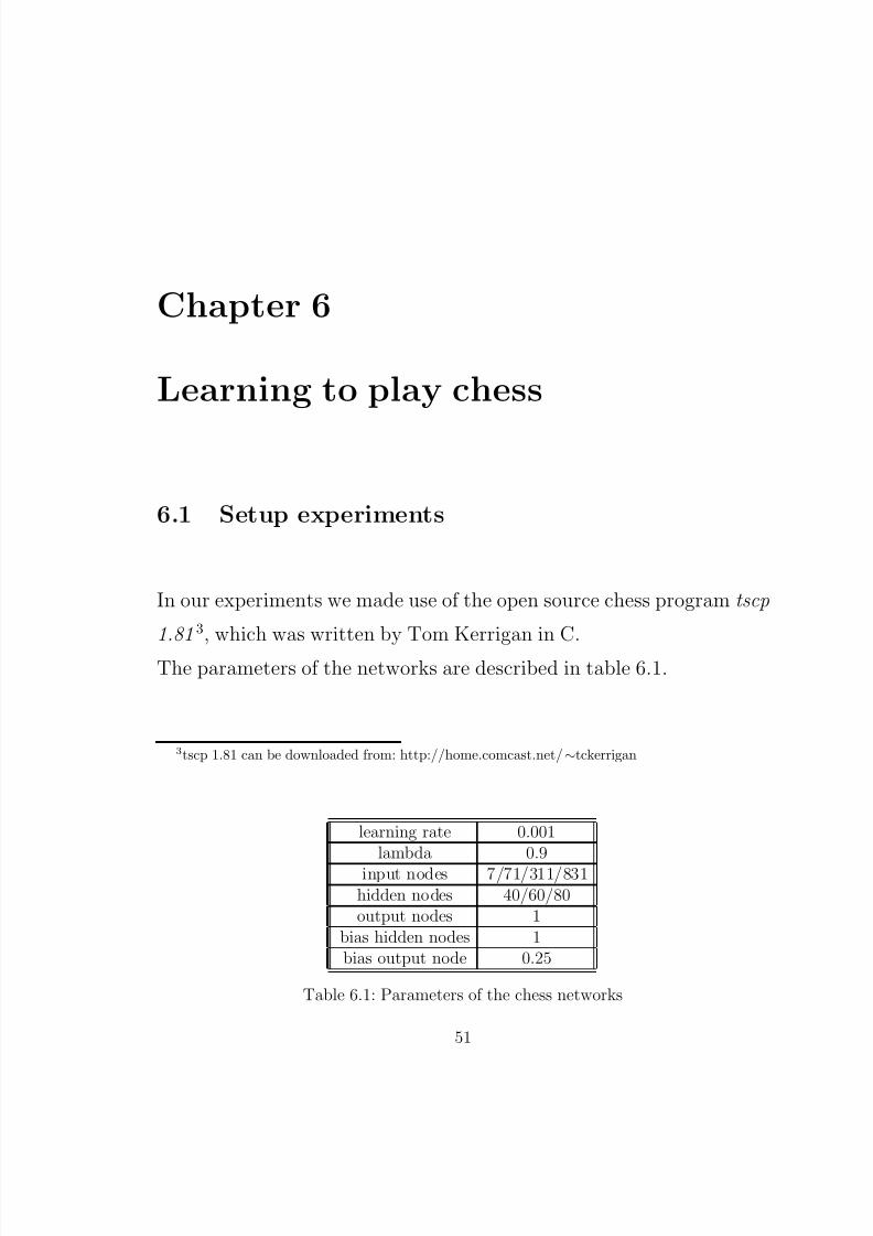
In our experiments we made use of the open source chess program tscp
1.81 3, which was written by Tom Kerrigan in C.
The parameters of the networks are described in table 6.1.
3tscp 1.81 can be downloaded from: http://home.comcast.net/∼tckerrigan
learning rate 0.001lambda 0.9
input nodes 7/71/311/831hidden nodes 40/60/80output nodes 1
bias hidden nodes 1bias output node 0.25
Table 6.1: Parameters of the chess networks
51

7/27/2019 Aprendizajereforzado Mannen
http://slidepdf.com/reader/full/aprendizajereforzado-mannen 65/91
52 Chapter 6. Learning to play chess
Piece Value in pawns
Queen 9Rook 5Bishop 3Knight 3Pawn 1
Table 6.2: Material values
6.2 First experiment: piece values
In the first experiment we are interested in the evaluation of a chessposition by a network, with just the material balance as its input. Most
chess programs make use of the following material values: According
to table 6.2, a queen is worth 9 pawns, a bishop is worth 3 pawns and
a bishop and two knights is worth a queen, etc. In our experiment the
network has the following five input features:
• white queens - black queens
• white rooks - black rooks
• white bishops - black bishops
• white knights - black knights
• white pawns - black pawns
The output of the network is the expected result of the game.
We tried 3 different networks in this experiment, one of 40 hidden nodes,
one of 60 hidden nodes and one of 80 hidden nodes. The obtained

7/27/2019 Aprendizajereforzado Mannen
http://slidepdf.com/reader/full/aprendizajereforzado-mannen 66/91
Chapter 6. Learning to play chess 53
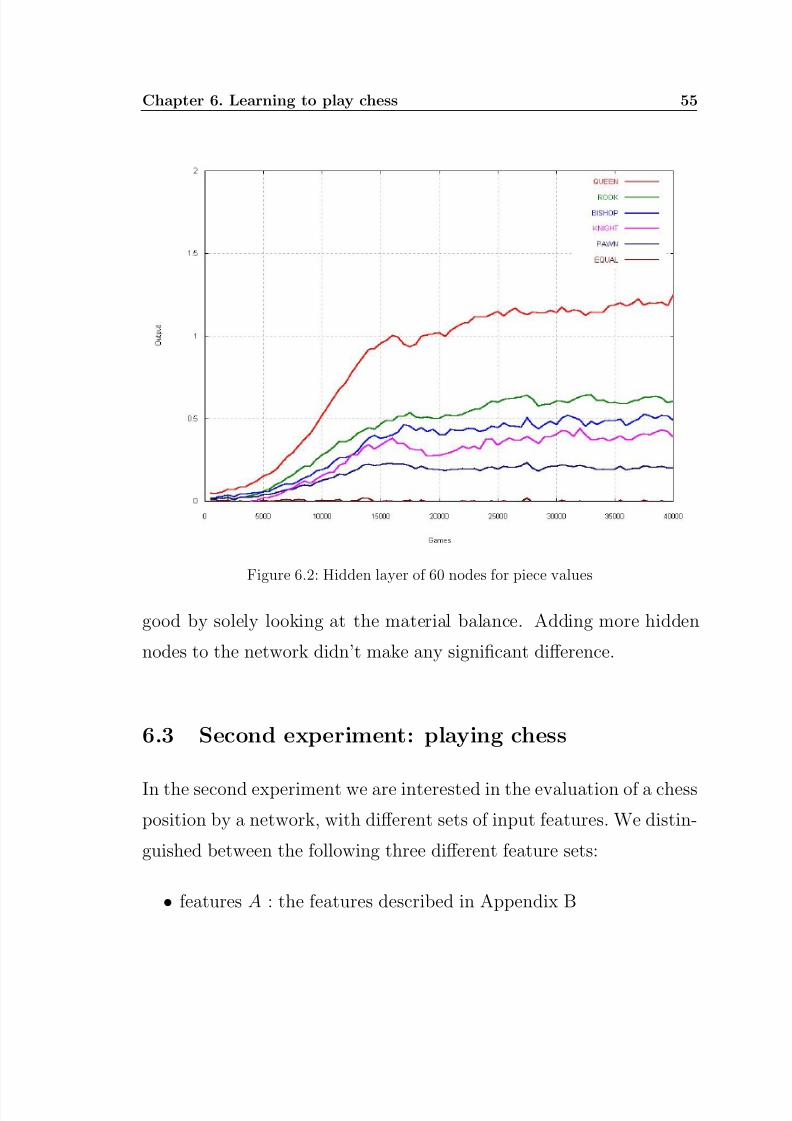
results are shown in figure 6.1, figure 6.2 and figure 6.3. These figures
show the output for six different cases:
• being a queen up
• being a rook up
• being a bishop up
• being a knight up
• being a pawn up
• equality
The figures show that the networks have a higher expectation to win
the game when they are a bishop ahead then when they are a knight
ahead. This is not as strange as it may seem, because more games
are won with a bishop more than a knight. For instance, an endgame
with a king and two bishops is a theoretical win. While an endgame
with a king and two knights against a king is a theoretical draw. The
network’s relative values of the pieces are not completely similar to the
relative values in table6.2. This is because the values in table6.2 don’t
say anything about the expectation to win a game. It is not that being
a queen up gives 9 times more chance to win a game than a pawn. It isalso important to note that being a rook up for instance, is not always
leading to a win. Games in the database where one player has a rook
and his opponent has two pawns often end in a draw, or even a loss for
the player with the rook. This is because pawns can be promoted to

7/27/2019 Aprendizajereforzado Mannen
http://slidepdf.com/reader/full/aprendizajereforzado-mannen 67/91
54 Chapter 6. Learning to play chess
Figure 6.1: Hidden layer of 40 nodes for piece values
queens when they reach the other side of the board. It is also possible
that a player is ahead in material at one moment in a game and later
on in the game loses his material advantage by making a mistake. So
the material balance in a game is often discontinuous.
Another thing is that one side can sacrifice material to checkmate his
opponent. In this case one side has more material in the final positionbut lost the game. Therefore the network is sometimes presented with
positions where one side has more material, while the desired output
is negative because the game was lost. We may conclude that the
networks were able to learn to estimate the outcome of a game pretty
7/27/2019 Aprendizajereforzado Mannen
http://slidepdf.com/reader/full/aprendizajereforzado-mannen 68/91
Chapter 6. Learning to play chess 55
Figure 6.2: Hidden layer of 60 nodes for piece values
good by solely looking at the material balance. Adding more hidden
nodes to the network didn’t make any significant difference.
6.3 Second experiment: playing chess
In the second experiment we are interested in the evaluation of a chess
position by a network, with different sets of input features. We distin-
guished between the following three different feature sets:
• features A : the features described in Appendix B

7/27/2019 Aprendizajereforzado Mannen
http://slidepdf.com/reader/full/aprendizajereforzado-mannen 69/91
56 Chapter 6. Learning to play chess
Figure 6.3: Hidden layer of 80 nodes for piece values
• features B : A and board position of kings and pawns
• features C : A and board position of all pieces(i.e., the raw board )
We trained seven different evaluation functions, which are described in
table6.3. All networks were trained on 50,000 database games. The
separated networks consist of three networks. They have a differentnetwork for each of the following game situations:
• positions in the opening
• positions in the middlegame

7/27/2019 Aprendizajereforzado Mannen
http://slidepdf.com/reader/full/aprendizajereforzado-mannen 70/91
Chapter 6. Learning to play chess 57
name program
a 1 network with features Ab 3 separated networks with features Ac 1 network with features Bd 3 separated networks with features Be 1 network with features C f 3 separated networks with features C g 1 linear network with features Bh handwritten evaluation function
Table 6.3: Program description
piece valuesdoubled pawnsisolated pawnspassed pawns
backward pawns4
rooks on semi open filerooks on open file
rooks on seventh rankking’s position
queen’s position
rook’s positionbishop’s positionknight’s positionpawn’s position
king’s safetycastling options
Table 6.4: Features of tscp 1.81
• positions in the endgame
The linear network is a network without an hidden layer(i.e., a percep-
tron).
The handwritten evaluation function is the function which is embed-
ded in tscp 1.81. It sums up the scores for the following features: We
7/27/2019 Aprendizajereforzado Mannen
http://slidepdf.com/reader/full/aprendizajereforzado-mannen 71/91
58 Chapter 6. Learning to play chess
a b c d e f g h
a x 5,5-4,5 5-5 3-7 8-2 8-2 5-5 4,5-5,5b 4,5-5,5 x 4-6 3,5-6,5 8,5-1,5 7-3 6-4 6-4c 5-5 6-4 x 4-6 8,5-1,5 7-3 5,5-4,5 6-4d 7-3 6,5-3,5 6-4 x 9-1 8-2 8-2 7-3e 2-8 1,5-8,5 1,5-8,5 1-9 x 4-6 2,5-7,5 3-7f 2-8 3-7 3-7 2-8 6-4 x 2-8 2,5-7,5g 5-5 4-6 4,5-5,5 2-8 7,5-2,5 8-2 x 6,5-3,5h 5,5-4,5 4-6 4-6 3-7 7-3 7,5-2,5 3,5-6,5 x
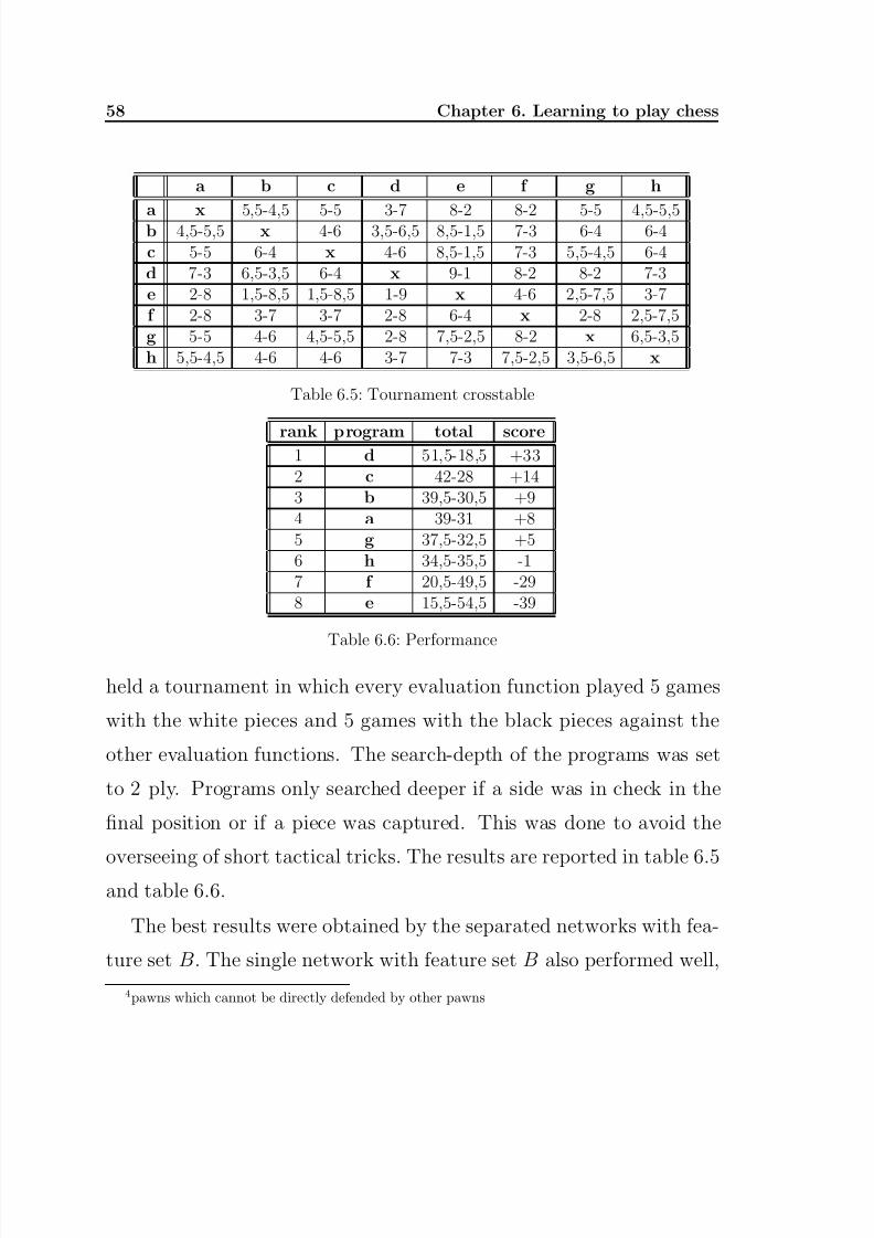
Table 6.5: Tournament crosstable
rank program total score1 d 51,5-18,5 +332 c 42-28 +143 b 39,5-30,5 +94 a 39-31 +85 g 37,5-32,5 +56 h 34,5-35,5 -17 f 20,5-49,5 -298 e 15,5-54,5 -39
Table 6.6: Performance
held a tournament in which every evaluation function played 5 games
with the white pieces and 5 games with the black pieces against the
other evaluation functions. The search-depth of the programs was set
to 2 ply. Programs only searched deeper if a side was in check in the
final position or if a piece was captured. This was done to avoid the
overseeing of short tactical tricks. The results are reported in table 6.5and table 6.6.
The best results were obtained by the separated networks with fea-
ture set B. The single network with feature set B also performed well,
4pawns which cannot be directly defended by other pawns
7/27/2019 Aprendizajereforzado Mannen
http://slidepdf.com/reader/full/aprendizajereforzado-mannen 72/91
Chapter 6. Learning to play chess 59
but its ’big brother’ yielded a much higher score. This is probably be-
cause it is hard to generalize on the position of kings and pawns during
the different stages of the game(opening, middlegame and endgame).
During the opening and middlegame the king often seeks protection in
a corner behind its pawns. While in the endgame the king can become
a strong piece, often marching on to the center of the board.
Pawns also are moved further in endgame positions than they are in the
opening and middlegame. Because the separated networks are trainedon the different stages of the game, they are more capable of making
this positional distinction.
The networks with feature set A also yielded a positive result. They
lack knowledge in the exact position of the kings and pawns on the
board. Therefore awkward looking pawn and king moves were some-
times made in their games.
The linear network made a nice result, but because it is just a linear
function it is not able to learn nonlinear characteristics of the training
examples. However, its result was still better than the result obtained
by the handwritten evaluation function, which scored slightly less than
50%.
The networks with the greatest amount of input features scored not
very well. This is probably because they have to be trained on muchmore games before they can generalize well on the input they get from
the positions of all pieces. Still, they were able to draw and win some
games against the other programs.
7/27/2019 Aprendizajereforzado Mannen
http://slidepdf.com/reader/full/aprendizajereforzado-mannen 73/91
60 Chapter 6. Learning to play chess
The separated networks yielded a better result than the single network
version. This can partly be explained by the fact that the separated
networks version was better in the positioning of its pieces during the
different stages of the game. For instance, the single network often put
its queen in play too soon. During the opening it is normally not very
wise to move a queen to the center of the board. The queen may have
a high mobility score in the center, but it often gives the opponent the
possibility for rapid development of its pieces by attacking the queen.It may be concluded that four of the six nonlinear evaluation functions
played better chess than a handwritten evaluation function after just
50,000 training games. It only took 7 hours to train evaluation function
d. This illustrates the attractiveness of database training in order to
create a reasonable evaluation function in a short time interval.
We end this chapter with an example win of evaluation function d over
the handwritten evaluation function.
[White ”d”] [Black ”h”] [Result ”1-0”]
1. c4 Nf6 2. Nc3 g6 3. d4 d5 4. cxd5 Nxd5 5. e4 Nxc3 6. bxc3 Nc6 7. d5 Ne5 8. Nf3
Nxf3+ 9. Qxf3 e5 10. Rb1 Bd6 11. Be3 O-O 12. Bd3 f6 13. O-O a5 14. Bh6 Re8 15. g4 a4
16. Be3 a3 17. Bc2 Ra6 18. Bd3 Ra8 19. h4 Ra5 20. Rb5 Rxb5 21. Bxb5 Bd7 22. Bxd7
Qxd7 23. Rb1 Rb8 24. Ba7 Rd8 25. Rxb7 Qc8 26. Rb8 Qd7 27. Rb3 c6 28. Be3 Be7 29.
c4 Qc8 30. Qe2 Bd6 31. c5 Be7 32. d6 Bxd6 33. cxd6 Rxd6 34. Bc5 Rd7 35. Rxa3 h6 36.
g5 fxg5 37. hxg5 hxg5 38. Qg4 Qe8 39. Rb3 Rd2 40. a4 Ra2 41. Ra3 Rxa3 42. Bxa3 c5
43. Bxc5 Qc6 44. Bb4 Qxa4 45. Qe6+ Kh7 46. Qf7+ Kh8 47. Qf8+ Kh7 48. Qe7+ Kh6
49. Kh2 Qc2 50. Qf8+ Kh5 51. Qh8+ Kg4 52. Qh3+ Kf4 53. Qe3+ Kg4 54. Qg3+ Kh5
55. Qh3# White mates 1-0
7/27/2019 Aprendizajereforzado Mannen
http://slidepdf.com/reader/full/aprendizajereforzado-mannen 74/91
Chapter 7
Conclusions and suggestions
7.1 Conclusions
We wanted to train several different chess evaluation functions(neuralnetworks) by using TD(λ) on a small set of database games. The goalwas to evolve evaluation functions which offered a reasonable level of play in a short period of training .The second experiment of the previous chapter showed that databasetraining is a good way to quickly learn a good evaluation function forthe game of chess. The use of partial raw board features proved to bebeneficial. It therefore can be argued that the evaluation functions withfull raw board features are the most promising versions on the long run,despite their relative bad results. In order to be able to generalize well
on the raw board features, they will probably need to be trained on alot more database games.The use of separated networks for the different stages of the game ledto better results than the use of single networks. This indicates that inorder to train an evaluation function for a problem domain, it is usefulto divide the available training examples into different categories.
61
7/27/2019 Aprendizajereforzado Mannen
http://slidepdf.com/reader/full/aprendizajereforzado-mannen 75/91
62 Chapter 7. Conclusions and suggestions
7.2 Further work
Finally, we will put forward three possible suggestions for future work:
1. Training on a larger amount of database games
2. Using self-play after database training
3. Selection of appropriate chess features for different game situations
First of all, as described in the previous section, it would be interestingto train the two evaluation functions with full raw board features on a
lot more examples. To be able to generalize on positions which differslightly in board position, but hugely in desired output the network hasto come across many examples.Secondly, the use of self-play after the training on database examplesmay also improve the level of play. The problem of self-play withoutdatabase training is that it is hard to learn something from randomplay. Database training offers a good way of training an initial evalu-ation function, because the training examples are, generally speaking,sensible positions.A third refinement is the use of different features for different game sit-uations. This helps to focus the evaluation function on what featuresare of importance in positions. For instance, in the middlegame, rooksincrease in strength when they are placed on a (semi) open file. How-ever, in an endgame with few pawns left or no pawns at all, this featureis of almost no importance. The input of this feature to the networktherefore should not influence the output. Hence, it will be better toskip this feature in this context.

7/27/2019 Aprendizajereforzado Mannen
http://slidepdf.com/reader/full/aprendizajereforzado-mannen 76/91
Appendix A
Derivation of the back-propagationalgorithm
The error E is half of the sum of the squares of the difference betweenthe activation of output node oi and the target output value for nodeoi.
E =1
2·
i
(ti − oi)2 (A.0.1)
The change in the weight from node i to node j should be proportional
to the gradient of the error with respect to that weight. η is the learningrate.
∆wij = η ·∂E
∂wij
(A.0.2)
By using the chain rule, the partial derivative ∂E ∂wij
is a product of partialderivatives.
∂E
∂wij
=∂E
∂hi
·∂hi∂wij
(A.0.3)
The second derivative in A.0.3 can be simplified to the activation of
node j.∂hi∂wij
=∂
∂wij
· (
k
wik · xk) = x j (A.0.4)
δ i is defined as:
δ i = −∂E
∂hi(A.0.5)
63
7/27/2019 Aprendizajereforzado Mannen
http://slidepdf.com/reader/full/aprendizajereforzado-mannen 77/91
64 Chapter A. Derivation of the back-propagation algorithm
The change in weight can now be defined in terms of the delta for the
destination node on the connection. We now need to know how tocalculate δ i for output and hidden nodes.
∆wij = η · δ i · x j (A.0.6)
Using the chain rule again, δ i is a product of partial derivatives.
δ i = −∂E
∂hi
= −∂E
∂oi·∂oi∂hi
(A.0.7)
The second of the derivatives in A.0.7 is just the derivative of the acti-
vation function(g) for the node.
∂oi∂hi
= gi(hi) (A.0.8)
For the first derivative in equation A.0.7, there are two cases: wherei is an output node and where it is a hidden node. If it is an outputnode, the derivative is the difference of the activation value and thetarget value.This is A.0.7 for output nodes:
∂E
∂oi= −(ti − oi) (A.0.9)
Combining A.0.8 and A.0.9 with A.0.7 gives:
δ i = (ti − oi) · gi(hi) (A.0.10)
For hidden nodes, we can use the chain rule to express the first deriva-tive in A.0.7 as a sum of products of partial derivatives. Node k isin the layer above the layer in which node i occurs. Using A.0.5, theexpression simplifies to the negative of the sum of the products of thedeltas of the nodes in the layer above i and the weights connecting i tothose nodes. This is A.0.7 for hidden nodes:
k
∂E
∂hk
·∂hk
∂oi=
k
∂E
∂hk·∂
∂oi·
j
wkj · oij (A.0.11)
7/27/2019 Aprendizajereforzado Mannen
http://slidepdf.com/reader/full/aprendizajereforzado-mannen 78/91
Chapter A. Derivation of the back-propagation algorithm 65
=
k
∂E
∂hk
· wki = −
k
δ k · wki (A.0.12)
δ i = (
k
δ k · wki) · gi(hi) (A.0.13)

7/27/2019 Aprendizajereforzado Mannen
http://slidepdf.com/reader/full/aprendizajereforzado-mannen 79/91
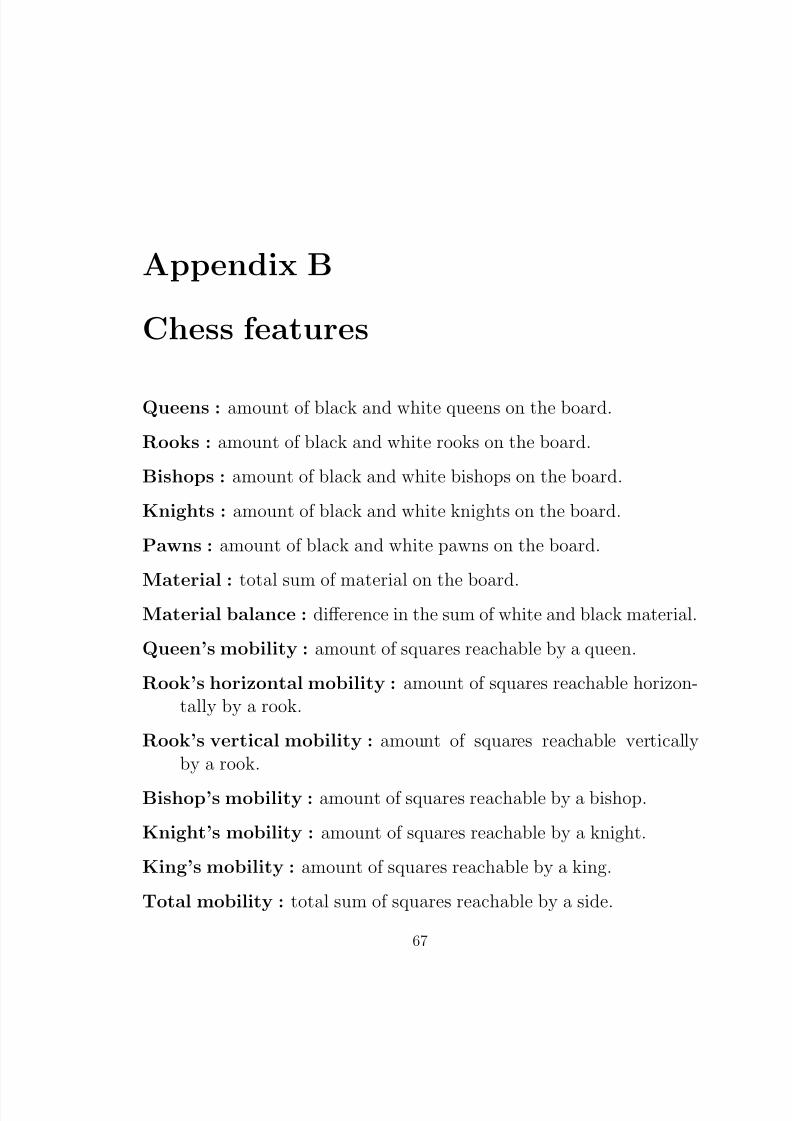
7/27/2019 Aprendizajereforzado Mannen
http://slidepdf.com/reader/full/aprendizajereforzado-mannen 80/91
Appendix B
Chess features
Queens : amount of black and white queens on the board.
Rooks : amount of black and white rooks on the board.
Bishops : amount of black and white bishops on the board.
Knights : amount of black and white knights on the board.
Pawns : amount of black and white pawns on the board.
Material : total sum of material on the board.Material balance : difference in the sum of white and black material.
Queen’s mobility : amount of squares reachable by a queen.
Rook’s horizontal mobility : amount of squares reachable horizon-tally by a rook.
Rook’s vertical mobility : amount of squares reachable verticallyby a rook.
Bishop’s mobility : amount of squares reachable by a bishop.
Knight’s mobility : amount of squares reachable by a knight.
King’s mobility : amount of squares reachable by a king.
Total mobility : total sum of squares reachable by a side.
67

7/27/2019 Aprendizajereforzado Mannen
http://slidepdf.com/reader/full/aprendizajereforzado-mannen 81/91
68 Chapter B. Chess features
Center control : amount of pawns occupying the squares e4, d4, e5,
d5.Isolated pawns : amount of pawns without a pawn of its own side on
an adjacent line.
Figure B.1: Isolated pawn on d4
In figure B.1 the pawn on d4 is the only isolated pawn.
Doubled pawns : amount of pawns, greater than 1, on 1 line.
In figure B.2 the pawns on e4 and e5 are doubled pawns.
Passed pawns : amount of pawns without an enemy pawn ahead of it on the same or an adjacent line.
In figure B.3 the white pawn on g5 and the black pawn on f5 arepassed pawns. The pawn on c5 has an enemy pawn ahead of it onan adjacent square, namely the pawn on b7. The pawn on b7 alsohas a pawn ahead of it, i.e., the pawn on c5.
Pawn forks : amount of pawns which attack two superior pieces. Infigure B.4 the pawn on e5 attacks the rook on d6 and the knighton f6.

7/27/2019 Aprendizajereforzado Mannen
http://slidepdf.com/reader/full/aprendizajereforzado-mannen 82/91
Chapter B. Chess features 69
Figure B.2: Doubled pawns
Figure B.3: Passed pawns on f5 and g5
Knight forks : amount of knights which attack two superior pieces.In B.5 the pawn on e5 attacks the rook on d6 and the knight on
f6.
Queens attacked : amount of queens attacked by inferior pieces.
Rooks attacked : amount of rooks attacked by inferior pieces.
Bishops attacked : amount of bishops attacked by inferior pieces.
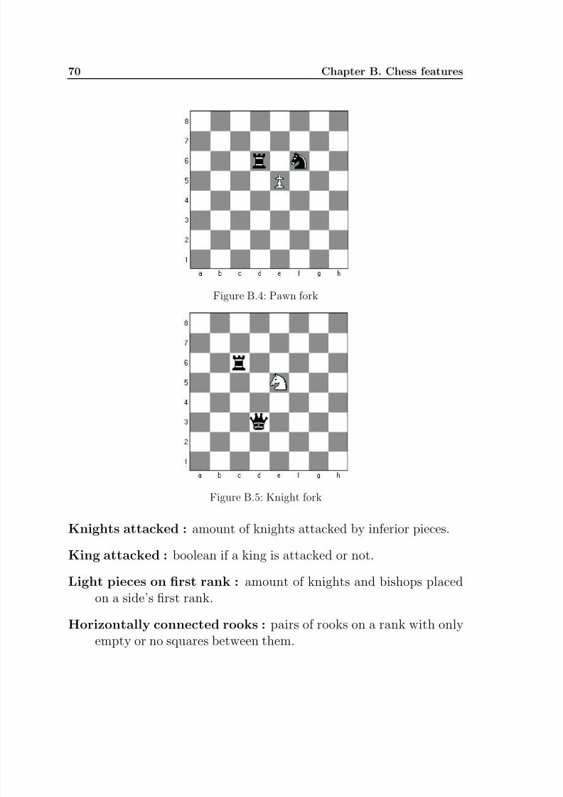
7/27/2019 Aprendizajereforzado Mannen
http://slidepdf.com/reader/full/aprendizajereforzado-mannen 83/91
70 Chapter B. Chess features
Figure B.4: Pawn fork
Figure B.5: Knight fork
Knights attacked : amount of knights attacked by inferior pieces.
King attacked : boolean if a king is attacked or not.
Light pieces on first rank : amount of knights and bishops placedon a side’s first rank.
Horizontally connected rooks : pairs of rooks on a rank with onlyempty or no squares between them.

7/27/2019 Aprendizajereforzado Mannen
http://slidepdf.com/reader/full/aprendizajereforzado-mannen 84/91
Chapter B. Chess features 71
Vertically connected rooks : pairs of rooks on a line with only empty
or no squares between them.
Rooks on seventh rank : amount of rooks on the seventh rank of aside. In figure B.6 both white and black have two rooks on ’the
Figure B.6: Rooks on the seventh rank
seventh rank’. From black’s viewpoint the black rooks on white’ssecond rank are on the seventh rank. Rooks on the seventh rankare often very powerful, especially two connected rooks. Theyhamper the opponent king in its movement and are a threat topieces which reside on that rank.
Board control : amount of empty squares controlled by a side. Infigure B.7 the black pawn on g4 controls the squares f3 and h3.The white knight only controls the square e2. The black pawn wins
control of the squares h3 and f3 over the knight because a pawnis worth less than a knight. The knight on its turn is in controlof the square e2 despite presence of the black rook on e8. This isbecause a rook is worth less than a knight. Generally speaking,the lower the rank of a piece, the greater its strength in controllingempty squares.

7/27/2019 Aprendizajereforzado Mannen
http://slidepdf.com/reader/full/aprendizajereforzado-mannen 85/91
72 Chapter B. Chess features
Figure B.7: Board control
Figure B.8: Connectivity
Connectivity : amount of connectedness between the pieces of a side.
In figure B.8 the connectedness of the white pieces is 7. The pawnon b2 covers the pawn on c3. The pawn on g2 covers the pawnon f3. The knight on e3 covers the pawn on g2 and the bishop onc2. The king on f2 covers the pawn on g2, the pawn on f3 and theknight on e3. There is no connectedness between the black piecesbecause no black piece is covered by another black piece.

7/27/2019 Aprendizajereforzado Mannen
http://slidepdf.com/reader/full/aprendizajereforzado-mannen 86/91
Chapter B. Chess features 73
King’s distance to center amount of squares a king is separated from
one of the center squares e4, d4, e5, d5

7/27/2019 Aprendizajereforzado Mannen
http://slidepdf.com/reader/full/aprendizajereforzado-mannen 87/91

7/27/2019 Aprendizajereforzado Mannen
http://slidepdf.com/reader/full/aprendizajereforzado-mannen 88/91
Bibliography
[Baxter et al., 1997] Baxter, J., Tridgell, A., and Weaver, L. (1997).
KnightCap: A chess program that learns by combining TD(λ) with
minimax search. Technical Report, Department of Systems Engineer-
ing, Australian National University.
[Beal, 1997] Beal, D. (1997). Learning piece values using temporal dif-
ferences. International Computer Chess Association Journal , 20:147–
151.
[Bellman, 1961] Bellman, R. (1961). Adaptive Control Processes: A
Guided Tour . Princeton University Press. Master’s thesis, Depart-
ment of Engineering and Computer Laboratory, University of Cam-
bridge.
[Ben-David et al., 1995] Ben-David, S., Kushilevitz, E., and Mansour,
Y. (1995). Online learning versus offline learning. In European Con-
ference on Computational Learning Theory , pages 38–52.
[Boyan, 1992] Boyan, J. A. (August 1992). Modular neural networks
for learning context-dependent game strategies . Cambridge, United
Kingdom. Master’s thesis, Department of Engineering and Computer
Laboratory, University of Cambridge.
75
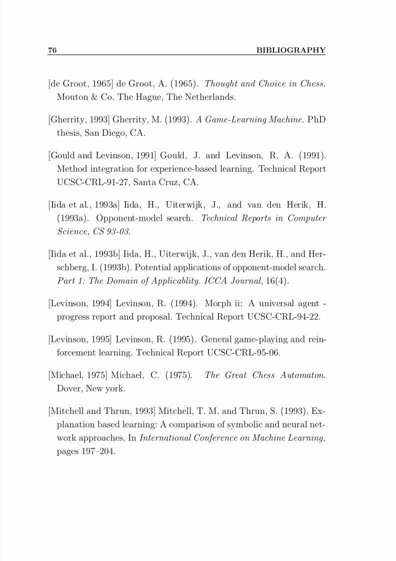
7/27/2019 Aprendizajereforzado Mannen
http://slidepdf.com/reader/full/aprendizajereforzado-mannen 89/91
76 BIBLIOGRAPHY
[de Groot, 1965] de Groot, A. (1965). Thought and Choice in Chess .
Mouton & Co. The Hague, The Netherlands.
[Gherrity, 1993] Gherrity, M. (1993). A Game-Learning Machine . PhD
thesis, San Diego, CA.
[Gould and Levinson, 1991] Gould, J. and Levinson, R. A. (1991).
Method integration for experience-based learning. Technical Report
UCSC-CRL-91-27, Santa Cruz, CA.
[Iida et al., 1993a] Iida, H., Uiterwijk, J., and van den Herik, H.
(1993a). Opponent-model search. Technical Reports in Computer
Science, CS 93-03 .
[Iida et al., 1993b] Iida, H., Uiterwijk, J., van den Herik, H., and Her-
schberg, I. (1993b). Potential applications of opponent-model search.
Part 1: The Domain of Applicablity. ICCA Journal , 16(4).
[Levinson, 1994] Levinson, R. (1994). Morph ii: A universal agent -
progress report and proposal. Technical Report UCSC-CRL-94-22.
[Levinson, 1995] Levinson, R. (1995). General game-playing and rein-
forcement learning. Technical Report UCSC-CRL-95-06.
[Michael, 1975] Michael, C. (1975). The Great Chess Automaton .
Dover, New york.
[Mitchell and Thrun, 1993] Mitchell, T. M. and Thrun, S. (1993). Ex-
planation based learning: A comparison of symbolic and neural net-
work approaches. In International Conference on Machine Learning ,
pages 197–204.

7/27/2019 Aprendizajereforzado Mannen
http://slidepdf.com/reader/full/aprendizajereforzado-mannen 90/91
BIBLIOGRAPHY 77
[Samuel, 1959] Samuel, A. L. (1959). Some studies in machine learning
using the game of checkers. IBM Journal of Research and Develop-ment , 3(3):210–229.
[Samuel, 1967] Samuel, A. L. (1967). Some studies in machine learn-
ing using the game of checkers ii - recent progress. IBM Journal of
Research and Development , 11(6):601–617.
[Schaeffer and Plaat, 1991] Schaeffer, J. and Plaat, A. (1991). Kas-
parov versus deep blue: The re-match. ICCA, 20(2):95–102.
[Shannon, 1950] Shannon, C. E. (1950). Programming a computer for
playing chess. Philosophical Magazine , 41(4):256–275.
[Sutton, 1988] Sutton, R. S. (1988). Learning to predict by the methods
of temporal differences. Machine Learning , 3:9–44.
[Tesauro, 1995] Tesauro, G. (1995). Temporal difference learning and
TD-gammon. Communications of the ACM , 38(3):58–68.
[Thrun, 1995] Thrun, S. (1995). Learning to play the game of chess.
Advances in Neural Information Processing Systems (NIPS), 7.
[Turing, 1950] Turing, A. M. (1950). Computing machinery and intel-
ligence. Mind , 49:433–460.
[Turing, 1999] Turing, A. M. (1999). Bbc radio talk. Machine Intelli-
gence , 15.
[Watkins, 1989] Watkins, C. (1989). Learning from delayed rewards .
PhD thesis, Cambridge, UK. PhD thesis, King’s college.
[Watkins and Dayan, 1992] Watkins, C. and Dayan, P. (1992). Tech-
nical note: Q-learning. Machine Learning , 8:279–292.

7/27/2019 Aprendizajereforzado Mannen
http://slidepdf.com/reader/full/aprendizajereforzado-mannen 91/91
78 BIBLIOGRAPHY
[Wiering, 1995] Wiering, M. (April 1995). TD Learning of Game Eval-
uation Functions with Hierarchical Neural Architectures . The Nether-lands. Master’s thesis, Department of Computer Systems, University
of Amsterdam.