MATHEMATICS OF OPERATIONS RESEARCHVol. 3, No, 3. August 197tlPrimed in U.S.A.

APPROXIMATIONS OF DYNAMIC PROGRAMS, I*t

WARD WHITT

Yale University and Belt Laboratories

A general procedure is presented for constructing and analyzing approximations ofdynamic programming models. The models considered are the monotone contraction opera-tor models of Denardo (1967), which include Markov decision processes and stochastic gameswith a criterion of discounted present value over an infinite horizon plus many finite-stagedynamic programs. The approximations are typically achieved by replacing the original stateand action spaces by subsets. Tight bounds are obtained for the distances between theoptimal return function in the original model and (1) the extension of the optimal returnfunction in the approximate mode! and (2) the return function associated with the extensionof an optimal pohcy in the approximate model. Conditions are also given under which thesequence of bounds associated with a sequence of approximating models converges to zero.

1. Introductioni and summary. If the state and action spaces in a dynamicprogramming model are large (infinite, for example), it is often convenient to use anapproximate model in order to apply a dynamic programming algorithm to obtain anapproximate solution. A natural way to construct an approximate model is to let thenew state and action spaces be subsets of the original state and action spaces; thendefine the new transition and reward structure using the transition and rewardstructure of the original model. Having defined the smaller model, calculate theoptimal return function and optimal policies for the smaller model and use them todefine approximately optima! return functions and approximately optimal policies forthe original model by a straightforward extension. An interesting question in thissetting is: what desirable properties do these extensions have for the original model? Itis the purpose of this paper to partially answer this question.

We begin in §2 with a definition of the model to be studied, which is the monotonecontraction operator model of Denardo (1967). We indicate how two such models canbe compared in §3 and give tight bounds on the difference between the optima! returnfunction in one model and the extensions from the other model. These comparisonscan be made when the state and action spaces of one model are subsets of thecorresponding state and action spaces of the other model, but also in other circum-stances. The special case in which the state and action spaces of one model are in factsubsets of the state and action spaces in the other model is discussed in §4. Severaldifferent methods for defining the transition and reward structure in the smallermodel are considered. In §5 we prove limit theorems. Under appropriate conditions, asequence of approximately optimal return functions generated from a sequence ofapproximate models converges uniformly to the optimal return function in theoriginal model. In §6 we consider a special case of the monotone contraction operatormodel^the standard stochastic sequential decision model. Finally, extensions arediscussed in §7. For example, corresponding results exist for finite-stage dynamicprograms, stochastic games and models with unbounded rewards.

* Received June 27, 1975; revised January 12, 1978.AMS 1970 subject classification. Primary 90C40.IAOR 1973 subject classification. Main: Markov decision programming. Cross references: Dynamic pro-gramming.Key words. Approximation, aggregation, dynamic programming, monotone contraction operators, fixedpoints, bounds.^ Partially supported by National Science Foundation Grant GK-38149 in the School of Organization andManagement, Yale University.

231Copyright ffi 1978, The Inslilute of Management Sciences

232 WARD WHITT

An account of related work in dynamic programming appears in Hinderer (1978)and Morin (1978). Our work was originally motivated by the discovery of an error inthe proof of the theorem in Fox (1973); a minor modification of the methods hereprovides a new proof. Thomas (1977) has applied the results here to study approxima-tions of capacity expansion models. The results here have been extended by Hinderer(1978), who also treats finite-stage dynamic programs. For related investigations inlinear programming, see Zipkin (1977) and references there.

2. Monotone contraction operators. Consider the dynamic programming modelintroduced by Denardo (1967) with the following notation. Let the state space be anonempty set S. For each s E S, let the action space be a nonempty set A^. Let thepolicy space A be the Cartesian product of the action spaces. Each element 8 in the setA is thought of as a stationary policy, specifying action d(s) to be taken in state s. LetV be the set of all bounded real-valued functions on S with the supremum norm:jt ll = sup{ji;(.?)| : s G S). The essential ingredient in the model specification is the

local income function h, which assigns a real number to each triple {s, a, v) with s E S,a G A^ and i: G K. The local income function h generates a return operator Hg on Vfor each 6 G A, i.e., [//5(t.)](5) = h{s, 8{s). v). We make three basic assumptions aboutthe return operators Hg\

(B) Boundedness. There exist numbers K^ and A'j such that \\H^v\\ < AT, + A 2ll' llfor all vG V and 8 E A.

(M) Monotonicity. If v > u in V. i.e., if v{s) > u{s) for all s E S, then H/^v > HgUin V for all 8 £ A.

(C) Contraction. For some fixed c, 0 < c < 1,

for all u,vEV and 8 G ^.The contraction assumption implies that Hg has a unique fixed point in V for each

5 e A. The unique fixed point of H^, denoted by Vg, is called the return functionassociated with policy 8. Let / denote the optimal return function., defined by f{s)— sup{(;g(.^) : S G A}. Let f be the maximization operator on K, defined by [F(L")](5)= sup{[//5(t-)](5) : S G A } . Perhaps the key structural property of this model is thatthe operator F inherits properties (B. M, C) and h a s / as its unique fixed point. Call apolicy 8 optimal if v^ = / a n d e-optional if v^{s) > f{s) - e for all s G S.By Corollary 1of Denardo (1967), there exists an e-optimal policy for each e > 0. We frequentlyapply the following basic result, which is Theorem 1 of Denardo (1967).

THEOREM 2.1. For all S e A and v G V,

V. - V and \\f-v\\ <{l - c) v - v

PROOF.

I- 1= \ k rrrr I

3. Comparing dynamic programs. Let (S, {A^, s E S), h, c) and (5 , {/I;, i"E S], h, c) be two dynamic programming models as defined in §2. We say that thesemodels are comparable and that the second is the [mage of the first if the followingmappings are defined: (1) a mapping/? of S onto S, (2) a mapping/? of A^ onto Ap^^yfor each s E 5, (3) a mapping e of S into S such that p{e[s]) = s for each SES and (4)a mapping e, of A ,^~. into A^ such that p{e^[a}) = a for each a E A ^^y and s E S. Given

APPROXIMATIONS OF DYNAMIC PROGRAMS, I 233

two comparable dynamic programs, define additional mappings: (1) e : V^ V withe{v){s) = v{p{s)) for each s E S, {2) p : V^V with p{v){h) = v{e[s]) for each sG S,(3) e : A ^ A with e{8){s)^ e^(8[p{s)]) for each 5 G 5 and (4)£ : A_- A with p{8){s)= p[8{e[s])] for each s E S. Note that _e(5) G A for every 5 e A. Note that thecomposition p " e is. the identity map on V and A, while e ° p on V and A is typicallynot. The models can be said to be in one-to-one correspondence if e <> /? is in fact theidentity map; we shall not dwell on this case. The "distance" between these twomodels can be expressed in terms of

K{v) = sup \h{s, a,, V) - h{p{s),p{a,),p{v))\, v E V, (3.1)

with K{v) understood to mean K(e[v]), ); G l . It turns out that K(v) is much moreuseful than K{v).

THEOREM 3.1. \\p{f)-f\\ < | | / - e{f)\\ < (1 - c)-'K{f).

PROOF._ The first inequality is obvious; we consider the second. Since ^ ^ < Ff = ffor each 8 e A, we can substitute e{f) for v in (3.1) to obtain

<e{f){s)+K{f)

for each s E S and 6 E A. Then, as a consequence of properties M and C plusinduction,

for all n and 8. Since \\H^v - v^\\^0 as « ^ o o ,

v,{s)<e{f){s)^{\~c)

for all 5 e A, so that

f{s)<e{f){s)^{\-c)-'K{f).

Similarly, for any e > 0, there exists a 6 G A such that

for al! s E S. Then, reasoning as above.

so that

f{s)>e{f){s)-{\-c)-'K{f).

THEOREM 3.2. For any 6 G A.

PROOF. Substituting e(5) for 8 and 0^ for v in (3.1) yields

\^ei.h)e{vi) - e{vs)\\ < K{v-^),

which implies the desired conclusion by virtue of Theorem 2.1. i

234 WARD WHITT

LEMMA 3.1. For all w, A:(i7) - K{v)\ <{c + c) u - v\

PROOF. By the triangle inequality.

K{u) < sup , e{u))

l . " ) l } .

so that K{u) < c|ie(w) - e(v)\\ + K(v) + c\\u - v

COROLLARY. If 8* is an e-optimal policy in A, then

^eiS'P) < m < V,^i.y{s) + 2(1 - c)-^K{f) + {\+ C)(l - .•)" '€,

for all s E S.

PROOF. Since £-(5*) E A, v^^,^ < / . The triangle inequality plus Theorems 3.1 and3.2 imply that

with Lemma 3.1 being used in the last step, iREMARKS. (1) It is easy to construct examples in which the inequalities here are

equalities.(2) Note that the bounds here involve K(v) rather than K(t:). The first part of the

proof of Theorem 3.1 can be imitated to obtain e{f){s) < f(s) + (I — c)^^K(f), butthe second part does not yield corresponding results. More generally, it is easy to

e(vxfiy orconstruct examples which show that it is not possible to boundIKs - i-Vo(fi)ll using K{v) in (3.1). Bounds on [|/— e{f)\\ in terms of / and differentdistance measure appear in §5 of Hinderer (1978).

(3) It is possible to examine the effect of replacing a good policy 5* by the "cruder"policy e ° p{8*). If 5* is t-optimal, then v^.^^^.p) > f(s) - (I - cy\3K(f) + 6e).

4. Smaller models. We now consider the special case of two comparable modelsin which S d S and (,j C A ^^ for each 5 E S. We can obtain the mapsp : A^^A ^^y e : S-*S and e^ : A^^^-^-^A, by constructing partitions of S and A^ foreach 5 G 5, and then selecting one point from each partition subset. In particular, let(Sy, J G / ) be a partition of subsets of 5, i.e., 5 = U ._, S', and 5, n \ =(f)ifi ^ iwith no restriction on the cardinality of /. Let S = (5,, / E / } be obtained by selectingone point from each subset in the partition of S. For each / G / and each s G 5"., let{A-,JGJ^) be partitions of nonempty subsets of A^, where again there is norestriction on the cardinality of the index sets 7,. We require that the cardinality of thepartitions of A^ be the same for all s G S , but it may vary with i. Moreover, thejthsubset A^ of A^^ is matched with theyth subset A^j of A^^ for all 5j, 52 E 5,. For s G S,and each / G /, let A^ = {a^^,J G J^) be new action spaces obtained by selecting onepoint a . from each subset Jl •. Let A^, A- and fl,y represent the quantities ^ , , / I , . anda^ . associated with states 5, G S. The mappings p and e here can be thought of asprojections and extensions: {V) p : S-~* S defined by p{s) = 5, for s E 5,, (2) p : A^

APPROXIMATIONS OF DYNAMIC PROGRAMS, I 235

-> Ap^^^ define_d by p(a^) = a^j if s E S, and a^ E A^j, (3) e : S^ S defined by e(5,) = 5,and (4) e^ : A^^^-^--^ A^ defined by e^(ay) = a if p{s) = s^. We have constructed thedefining mappings from partitions and identified points in each partition subset, butwe can go the other way. The mappings determine partitions and identified points ineach partition subset, e.g., S^ = p^\s,) = {s E S : pis) = s^} for .v. G S a.nd a^j = e^a^j)

To complete the definition of the smaller model, we need to define a local incomefunction h such that the induced operators H^ on V satisfy properties B, M, C.Motivated by the desire to have the small model be a simple approximation for theoriginal model, we are led to the definition

h (s^, a-, v) = his-, a^. ^{^)) (4.1)

for all a- G A-, Sj & S, v E V. Obviously, the associated return operators H^ on Vsatisfy B, M, C with a contraction modulus less than or equal to c.

There are, of course, many other possible definitions for the approximate localincome function h. For example,

sup h{s,a^,e(v))+ inf h{s,a^,e{v)) (4.2)

and

hjiS:, a-, V) ^^ I ' ' 1 ^ , fl,, £?(u)) dii.:(s, aA (4-3)

where B^ = {(s, aj) : s E 5,, a^ E A^}, (i-j is a probability measure on B.j such as theuniform distribution (when applicable) and the appropriate measurability assumptionsare made so that the integral makes sense. Obviously (4.1) is a special case of (4.3).Obviously A'(t;) in (3.1) as a function of h is minimized for every fixed v by (4.2). Inboth (4.2) and (4.3) properties B, M, C hold with a contraction modulus less than orequal to c.

Recall that the theorems in §3 apply to all such smaller models, but bo th /and K(v)change from model to model, so that the bound K(f) varies in an unpredictable way.To obtain a bound applicable to a variety of models, let

Liv) = sup sup |/?(5', a^., v) - his", a^-, v)\ (4.4)

for any u G K. As with K(v) in (3.1), we write L(i3) for L(e(v)). As an immediateconsequence of (3.1) and (4.4), we obtain

LEMMA 4.1. / /

inf h{s, a,, v) < h (s,, a,^,p(v)) < sup h(s, a,, v) (4.5)

for all i and J, then K(v) < T(v).

Note that (4.5) is satisfied for v = e(v) and the choices of ^~in (4.1)-<4.3).REMARK. It is interesting that any of these smaller models {§, {A^, s G S], h, c)

can be embedded in the setting of the larger model by setting 8Xs) = 8[p(s)] and

h'is, 6'isy v) = h{p{sy E[p{s)lp{v))

236 WARD WHfTT

for any s G S, 8 E K and v E V. (Note that 8' might not be in A.) Operators H^. canthen be defined on V in the usual way by [Hl(v)](s) = h'(s, 8'{s), v). This embeddingis the symmetric extension introduced in §7 of Denardo [2]. The primed model here isspecified completely by^5" = 5, A'^ = Ap^^y for s E S, and h' above. It is elementarythat Vs' = e(vg) for al! 6 E A, cf. Theorem 5 of [2]. Hence^ the new model (S',{A'^, sE S'], h') is a representation of the smaller model (S, {^,, / G / } , h) with the samestate space as the larger model. Moreover, the theorems in §3 comparing the models(5, [A^, s G S], h) and (.S", {A-, i E I], h) are natural generalizations of the symmetrytheorem in §7 of [2], comparing the models (S ' , {A'^, s E S'}, h') and (S, {A^, iEl), h).

5. Limit theorems. Given a dynamic programming model as defined in §2, weshould expect that it is possible to construct a sequence of approximating smallermodels as defined in §4 such that the smaller models become better and betterapproximations for the original models as the partitions associated with the smallermodels become finer and finer. In particular, we should hope that the sequences ofreturn functions {£„(/„)} and {v^ /§.)} generated from the sequence of smaller modelsconverge to the optimal return function / . The results in this section apply to al! the!oca! income functions in (4. l)-(4.3); we only assume h has modulus c and (4.5) issatisfied for all v E I . In fact, it is only used for v = p{f)-

THEOREM 5.1. //(4.5) holds for v = e^ " p^if) for all n, then there exists a sequenceof finite partitions of S and A^, s E S, such that lim^^^

REMARKS. (1) The proof is constructive, but the construction is of limited practicalvalue because the optimal return function / is used. This does suggest a heuristicmethod: first make a rough estimate o f / and then apply the construction using it. Forexample, use <?„_[(/„_[) to define the partitions in the nth approximating model with

(2) By Theorem 3.1 and Lemma 4.1, Theorem 5.1 implies that j | / — ^/,(//j)ll~*O, butthis is shown directly in the proof.

The proof uses the following lemma, which applies to a single approximate model.For any v E V, let

0}{v) = s u p ( | t ; ( / ) - v { s " ) \ : s \ s" E S . , i E I ) . (5.1)

LEMMA 5.1. Assume (4.5). / / w( / ) < e and 8' is any policy in A such that

sup{\h{s, a,,f) -f{s,)\ -.iELsE S,. a, G A,^. S'(s,) = a,^] < t,

then

(a)

\\f-p(f)\<{\+c){\-cy't.and

K/)-/ 2(1 -

PROOF OF LEMMA 5.1. (a) To simplify notation, let Sup represent the supremumover i E I, s E S, and a^ E A^j, where S'(s^) = a^j. By (4.5) for v = e ° p(f), the triangleinequality and the two conditions.

, «,, e o pif)) - h{s, «,,/)! + Sup\h{s. a,,f) - / ( . ,

< c\\e o p(f) -f\\ + e< cw(/) + € < (1 - c)£,

which, with Theorem 2.1, implies that

' {\+ c){\ - c)- 'e .

APPROXIMATIONS OF DYNAMIC PROGRAMS, I 237

(b) By (4.5) and the first condition, for any 5 E A with 6(5,) = a^j.

sup his,a^,e o pif))^ sups^S, J e s,-

< sup fis) + C€< Pif)is,) + (1 + c)e,

SO that, by the argument used in Theorem 3.1,

vsi^d<Since 6 was arbitrary.

On the other hand, by part (a).

(c) By the triangle inequality,

Mh-fW < l l^( /)- ^ ^/'C/)!! + We-'Pif)-f\\

PROOF OF THEOREM 5.1. Since/ E V, property B implies there exists a constant Ksuch that \his, 8isyf)\ < K for all 5 E 5 and 6 E A. Hence, for each « > 1, a finitepartition of nonempty subsets of the set of all state-action pairs can be constructed byletting

Bk = {{s,a) : s E S, a E A^, k/n < his, a,f) <{k + \)/n], -oo <k < oo,

where we suppress the dependence on n. For each s E S and subset B^, define the5-section of B,^ in the usual way as

Associate with each state s the necessarily finite set / of indices for which the5-sections are nonempty, i.e.,

h={k:iB,)^^0].

Define an equivalence relation on S by saying that 5, is equivalent to 2 if / = I,. Let(^i, . . . , 5^} be the finite partition of equivalence classes in S. Form the state spaceS of the smaller model by selecting one point 5, from each subset Sj of this partition ofS. For eaeh / and s G 5*,, use the subcollection of fi^ subsets for k E I^ to form thepartitions of the action space A^. For example, suppose one such subcollection hasbeen relabeled as {S , 1 < j < k}. Then let

A^j = {aE A, : (.9, a) E B^), \ < J ^ k, s E S,.

Then select one point a^j from each subset A^j associated with the subcollection{BJ, 1 < 7 < k). Let the projection be defined as p(s) = s- and p(aj = a^^ if s E S^and a^ G A^j. After reintroducing n, this construction yields L^if) <«"" ' . cf. (4.4).t o^ ( / )<«- ' , c f . (5.1), and

snp[\his, a,,f) -f(s^)\ : / G /, 5 G S,. a, E A,^, S'is,) = a,^} < n-\

where 8'is^) attains the maximum over y of his,,ajj,f), so that both conditions inLemma 5.1 hold with e < n^K Finally,

238 WARD WHITT

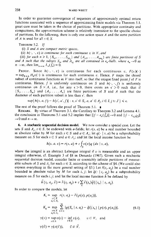
In order to guarantee convergence of sequences of approximately optimal returnfunctions associated with a sequence of approximating finite models via Theorem 5.1,great care must be taken in the choice of partitions. With appropriate continuity andcompactness, the approximation scheme is relatively insensitive to the specific choiceof partitions. In the following, there is only one action space A and the same partitionof A is used for all s E S.

THEOREM 5.2. / /

(i) 5 and A are compact metric spaces,(ii) h[-, -.v) is continuous for each continuous t in V, and

(iii) for each n> \. {5,,|, . . . , S^ .J and {A„•^ A^^J are finite partitions of Sand A such that the subsets S^- and A^- are all contained in ^^-balls, where £„ 0 asn^cc, then lim^^^ L^(l) = 0.

PROOF. Since /?(•, -. v) is continuous for each continuous v, F[c)[-)= supsei//^t;(-) is continuous for each continuous t-. Hence, F maps the closedsubset of continuous functions in V into itself, so that the unique fixed point / of F iscontinuous. Hence. / is uniformly continuous on S and h[-, •,f) is uniformlycontinuous on SxA, i.e., for any « > 0, there exists an e ' > 0 such that if{ 5 i , . . . , S ^ } and {A^ A^} are finite partitions of S and A such that thediameter of each partition subset is less than e'. then

sup{/i(5, a,f)- h[s',a',f)\ : s, s' E S^,a, a' E Aj, i E I,f Ej] < e.

The rest of the proof follows the proof of Theorem 5.1. iREMARK. By virtue of Theorem 3.1, the Corollary to Theorem 3.2 and Lemma 4.1,

the conclusion in Theorems 5.1 and 5.2 implies that | | / - e^(/,)j|-»O and | | / - v^^g.-jW-^0 and «-*Go.

6. A stochastic sequential decision model. We now consider a special case. Let thesets S and A^, s E S, he endowed with a-fields; let r[s, a) be a real number boundedin absolute value by M for each s E S and a G A^; let q[- {s, a) be a subprobabiiitymeasure on S for each s G S and a E A- and let the local income function be

h{s, a, v) - r{s, a) + c ( v[x)q [dx | 5, a).

where the integral is an abstract Lebesgue integral if v is measurable and an upperintegral otherwise, cf. Example 3 of §8 in Denardo (1967). Given such a stochasticsequential decision model, consider finite or countably infinite partitions of measur-able subsets of S and A^ for each s G S, according to the scheme of §4. (We could alsoexpress everything in the more general setting of §3.) Let r(s^, a,.) be a real numberbounded in absolute value by M for each i, J; let q[- \ s-, a^) be a subprobabiiitymeasure on S for each /,y; and let the local income function h be defined by

j j s,,n

In order to compare the models, let

K,= sup

} \p(s),p[a^,))l (6.1)

y[v) = supi;(i) - inf 1 (5), v G V, and

y[v)=y[e{v)), 6EV.

APPROXIMATIONS OF DYNAMIC PROGRAMS, I 239

We now obtain a bound for K(v) in (3.1) using K^, K^ and y in (6.1).

c\\v K^.THEOREM 6.1. (a) For any vEV, Kiv) < ^

(b) / / q(S I s, a,) = qiS | pis), p{a,)) = 1 for all a, G A, and s E S, then

K{v)< K,+ cyiv)K^/2.

Theorem 6.1 yields an obvious bound on K(f) which does not require that we solveeither problem. For this a priori bound, let

7;= sup ?{pisypia^))- inf ?ipisypia,)y (6.2)

COROLLARY, (a) c(\ -() if) K ^s. a,) = qiS | pis), p(a^)) = 1 for all a, G A^ and s E S, then(b)

PROOF OF THE COROLLARY, (a) Note that Ili; !! < (I - c)" ' | | r (- , 5(-))ll <(1 - c)'"'W. (b) Note that y( / ) < (1 - c)"'y?- •

In the proofs of Theorems 6.1 and 6.2 we use the fact that the upper integralfg V dfi is countably additive as a function of B. We first state a lemma which doesnot exploit partitions.

LEMMA 6.1. / /fi , and iij are two finite measures on S, then

PROOF. Observe that the upper integrals satisfy

d}Li- (vdiij<s&S

min

— min{

— min( inf 1

To obtain the inequality in the other direction, change the subscripts of |x^ and ti-2- •We now exploit the partitions. For this purpose, let

y^(t:) = sup v(s) - inf vis) and

s)\.

Note that w(r) = sup^ y^(t;) for w in (5.1). Let

M= 1

i ^ measures on 5.where jx, and ^2 ^^

LEMMA 6.2. (a) / / /x, and lU are two finite measures on S. then

fvd^^- (v• 'S •'S

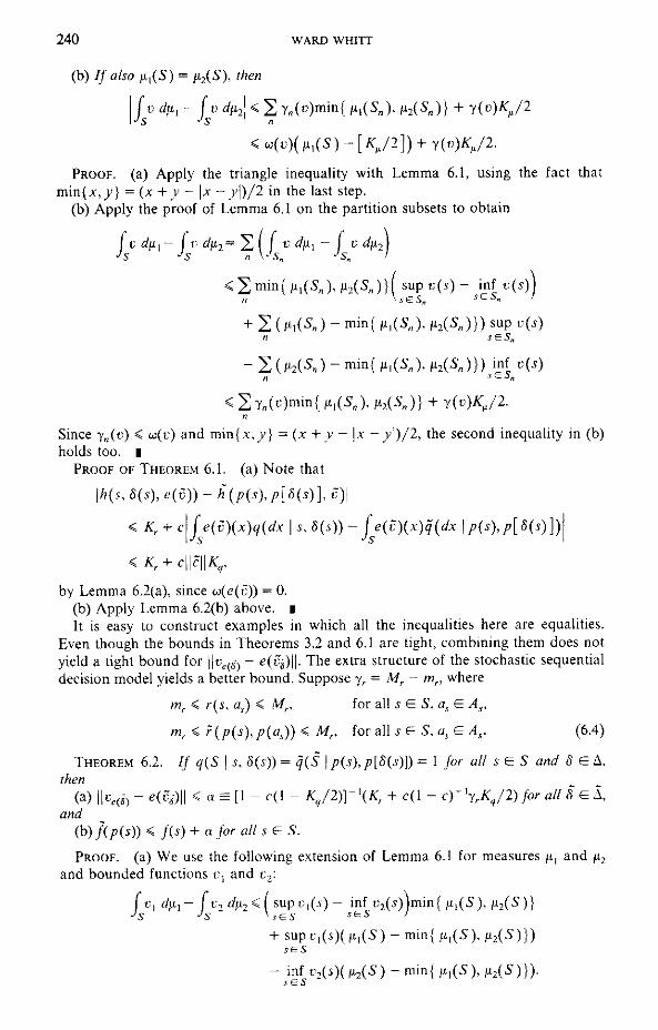
240 WARD WHITT

(b) If also jU|(S) = ii2{S), then

PROOF, (a) Apply the triangle inequality with Lemma 6.1, using the fact thatmin(ji:,/} ={x-\- y '-\x -- y\)/2 in the last step.

(b) Apply the proof of Lemma 6.1 on the partition subsets to obtain

f ^ I C • f J \I i; du.2— 2^\ \ ^ du, — \ V dn21

- min

s u p v{s) - in f v{s)\

})supu(.y)

{ l i i . l ^2{n)]) {)

M5J) + y{v)KJ2.n

Since y^{v) < w(f) and min{x,/} = {x + y - \x -y\)/2, the second inequality in (b)holds too. I

PROOF OF THEOREM 6.1. (a) Note that

\h{s,8{s),e{v))-^h{p{s),p[8{s)lv)\

(e{v){x)q{dx\s,d{s))-(e{v){x)q{dx \p{s),p[8{s)])K+c

by Lemma 6.2(a), since <^{c(v)) = 0.(b) Apply Lemma 6.2(b) above, iIt is easy to construct examples in which all the inequalities here are equalities.

Even though the bounds in Theorems 3.2 and 6.1 are tight, combining them does notyield a tight bound for \\v^0-) - e{Vg)\\. The extra structure of the stochastic sequentialdecision model yields a better bound. Suppose y^= M^- m^, where

^ < r{s, a^) < M,, for al! s G S,a^

^ < r{p{s), p{a^)) < M^, for all s G S.a^ (6.4)

T H E O R E M 6 . 2 . If q(S \ s, 8{s)) = q{S \ p{s), p[8{s)]) = 1 for all s G S and SEX

thenor all 8 G I,(a) lk,(5) - e{vM <a = [l-c{\- KJDY \K, + c(l - c) J

and(b) /(;'(^)) < /(^) + « lor all s G S.

PROOF, (a) We use the following extension of Lemma 6.1 for measures /x, and 1X2and bounded functions v-^ and Cj:

I \

i/fi2< supi ) , ( .v ) - inf t,-2(5)

min

'mf

APPROXIMATIONS OF DYNAMIC PROGRAMS, I

Moreover, if Uj is constant, then

Applying these inequalities on the partition subsets, we obtain

,- - / c,\ y>f .!^-\i c\ — t-{ P £>( Si \( vW -U ^ I t' - (

241

l 8[p[s)]) - c

s, e[8){s))

,} \p[s), 8[p[s)])

:,(5,(5)(l - Q[s, 6 )

-cmle[6i)[s){l-Q[s,8)),

where

— I — T "

Since Q[s, 8) > I - KJ2,

( l - c ) " ' m , <

s,] \p[s),

1= 1

s, e[8)[s)) -

and e[vi)[s)<{\ -

Similarly, e[v'^)[s) — v^^3^j[s) has the same upper bound, so that

(b) For any e > 0, there is a 6 E A such that Vg[p[s)) > f[p[s)) — €. Then

f[p{s)) < H{P{S)) + € < tV(5)(^) + « + £ < f[s) + « + £. I

REMARKS. It is easy to construct an example showing that the bound in Theorem6.2 is tight. We have not yet determined a tight upper bound for f[s) - f[p(s)).

7. Extensions. (1) The contraction assumption (C) can be replaced by the A'-stage contraction assumption, cf. §5 of Denardo (1967). For example, suppose

HgU - Hgv\\ < m||w - i;|| a n d Hl'u < c u - v for all A, where c < 1but not necessarily m < 1; then the bound in Theorem 3.1 becomes (1 + m + • • • +m'^~')(l — c)~^K[f). This extension includes many A'-stage dynamic programs (usu-ally with m = 1 and c = 0). The representation of finite-stage dynamic programs asmonotone contraction operator models is facilitated by including the stage as part ofthe state description. For example, after this modification, there is no loss ofgenerality in considering only stationary policies. Approximations of finite-stagedynamic programs are studied directly by Hinderer (1978).

(2) Corresponding theorems hold for the case of unbounded rewards, cf. Wessels(1977). For example, suppose b : S-^R, jx : S-*[0, oo).

= iv sup\[v[s)- b[s)]/ii[s)\< oo

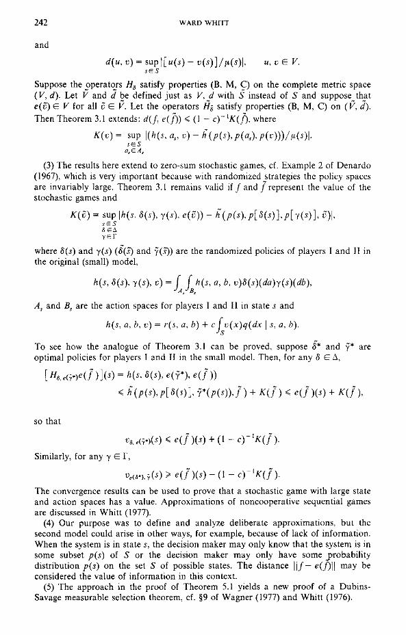
242 WARD WHITT

and

d{u, v) = sup\[u{s) - v{s)]/{i{s)\, u,vEV.sES

Suppose the operators H^ satisfy properties (B. M, C) on the complete metric space(V, d). Let V and d be defined just as V, d with 5 instead of S and suppose thate(v) E V for all v E V. Let the operators Hg satisfy properties (B, M, C) on (V, d).Then Theorem 3.1 extends: d{f, e{f)) < (1 - cy^K{f), where

K{v)= sup

(3) The results here extend to zero-sum stochastic games, cf. Example 2 of Denardo(1967), which is very important because with randomized strategies the policy spacesare invariably large. Theorem 3.1 remains valid if / and / represent the value of thestochastic games and

K{v) = sup \h{s. 8{sl y{sl e{v)) - h{p{s),p[8{.s)lp[y{s)],S

yer

where 8{s) and y{s) {8{s) and 'y(^) are the randomized policies of players I and Ii inthe original (small) model,

h{s, 8{s), y{s), v)= ( ( h{s, a, b, v)S{s){da)y(s){db),•'A/B,

A^ and B^ are the action spaces for players I and II in state s and

h[s, a, b, v) = r{s, a, b) + c j v(x)q(dx \ s, a, b).

To see how the analogue of Theorem 3.1 can be proved, suppose 5* and f* areoptimal policies for players I and I! in the small model. Then, for any 5 G A,

= h{s, 5(5), e(y*), e(f~))

so that

Similarly, for any y ET,

The convergence results can be used to prove that a stochastic game with large stateand action spaces has a value. Approximations of noncooperative sequential gamesare discussed in Whitt (1977).

(4) Our purpose was to define and analyze deliberate approximations, but thesecond model could arise in other ways, for example, because of lack of information.When the system is in state s, the decision maker may only know that the system is insome subset p(s) of S or the decision maker may only have some j^robabilitydistribution p(s) on the set S of possible states. The distance ||/— e(f)\\ may beconsidered the value of information in this context.

(5) The approach in the proof of Theorem 5.1 yields a new proof of a Dubins-Savage measurable selection theorem, cf. §9 of Wagner (1977) and Whitt (1976).

APPROXIMATIONS OF DYNAMIC PROGRAMS, I 243

Acknowledgment. I am grateful to Eric Denardo, Karl Hinderer, Arie Hordijk,Uriel Rothblum and Frank Van der Duyn Schouten^ for helpful comments andcorrections. Theorems 3.1 and 3.2 in their present form are due to Eric Denardo.

References[1] Bertsekas, D. P. (1975). Convergence of Discretization Procedures in Dynamic Programming. IEEE

Trans. Automatic Control. 20 415-419.[2] Denardo, E. V. (1967). Contraction Mappings in the Theory Underlying Dynamic Programming.

SIAM Rev. 9 165-177,[3] Fox, B. L. (1973). Discretizing Dynamic Programs. J. Optimization Theory Appl. 11 228-234.[4] Hinderer, K. (1978). On Approximate Solutions of Finite-Stage Dynamic Programs. Proceedings of the

International Conference on Dynamic Programming, Vniversity of British Columbia, Vancouver. M.Puterman (ed.). To appear.

[5] Morin, T. L. (1978). Computational Advances and Reduction of Dimensionality in DynamicProgramming: A Survey. Proceedings of the International Conference on Dynamic Programming,University of British Columbia, Vancouver. M. Puterman (ed.). To appear.

[6] Thomas, A. (1977). Models for Optimal Capacity Expansion. Ph.D. Dissertation, School of Organiza-tion and Management, Yale University.

[7] Wagner, D. H. (1977). Survey of Measurable Selection Theorems. SIAM J. Control Optimization 15859-903.

[8] Wessels, J. (1977). Markov Programming by Successive Approximations with Respect to WeightedSupremum Norms. J. Math. Anal. Appt. 58 326-335.

[9] Whitt, W. (1976). Baire Classification of Measurable Selections of Extrema.[10] , (1977). Representation and Approximation of Noncooperative Sequential Games.[11] Zipkin, P. H. (1977). Aggregation in Linear Programming. Ph.D. Dissertation, School of Organization

and Management, Yale University.

BELL LABORATORIES, HOLMDEL, NEW JERSEY 07733