Approximations for the distributions of bounded … for the distributions of bounded variation...

Approximations for the distributions of

bounded variation Levy processes

Jose E. Figueroa-Lopez

Department of StatisticsPurdue University

W. Lafayette, IN 47907, USA

Abstract: We propose a feasible method for approximating the marginaldistributions and densities of a bounded variation Levy process using poly-nomial expansions. We provide a fast recursive formula for approximatingthe coefficients of the expansions and estimating the order of the approxi-mation error. Our expansions are shown to be the exact counterpart of suc-cessive approximations of the Levy process by compound Poisson processespreviously proposed by, for instance, Barndorff-Nielsen and Hubalek (2008)[Probability measures, Levy measures, and analyticity in time. Bernoulli,3(14), 764-790] and others, and hence, give an answer to an open problemraised therein.

AMS 2000 subject classifications: 60G51, 60F99.Keywords and phrases: Levy processes, small-time expansions of distri-butions, transition distributions, transition density approximations.

1. Introduction

In this paper we consider a driftless pure-jump Levy process X = (Xt)t≥0 ofbounded variation, or equivalently expressed in terms of the generating triplet(σ2, b, ν) of X , a Levy process such that

(i) σ = 0, (ii)

∫

{|x|≤1}

|x|ν(dx) < ∞, (iii) b0 := b−

∫

{x≤1}

xν(dx) = 0.

(1.1)We also assume that ν admits a smooth Levy density s : R\{0} → [0,∞) (see,e.g., Sato (1999) for the terminology and background on Levy processes).

During the last decade Levy processes have regained popularity as the under-lying source of randomness driving the dynamics of different physical phenomenasuch as asset prices and weather measurements. One drawback in working witha Levy process {Xt}t≥0 is that in general neither their marginal distributionfunctions Ft(x) = P(Xt ≤ x) nor their marginal densities pt(x) = F ′

t (x) areeasily computable. In some cases there do exist closed formulas for the marginaldensities in terms of special functions, but in general, one needs to rely on nu-merical approximations to find these quantities. For instance, in the so-calledCGMY model of Carr et al. (2002), the Levy triplet (σ2, b, ν) of the process issuch that

b ∈ R, σ = 0, and s(x) =Ce−Gx

x1+Y1{x>0} +

Ce−M|x|

|x|1+Y1{x<0}, (1.2)

1

Figueroa-Lopez/Approximations for Levy processes with bounded variation 2

with 0 ≤ Y < 2, and positive C, G, and M . The above model was previouslyconsidered by Koponen (1995) (see also Novikov (1994)) under the name ofthe “truncated Levy flight”, while its application for financial modeling wasalso proposed in Cont et al. (1997) and Matacz (2000)1. In the case of Y = 0,the CGMY model reduces to the well-known variance Gamma process, whosemarginal densities admit a closed formula in terms of modified Bessel functionsof the second kind (cf. Carr et al. (1998)). However, there is no closed formulafor any other value of Y and, in order to compute the marginal density, onewould have to use numerical methods such as fast Fourier transforms combinedwith an inversion formula for the characteristic function as proposed in, e.g.,Carr et al. (2002), Section 5.1.

A well-known method of construction for Levy processes is via the limit ofcompound Poisson processes (see, e.g., Sato (1999), Corollary 8.8). In the caseof an infinite-jump activity subordinator (σ = 0, ν(R) = ∞, ν((−∞, 0)) =0, and

∫∞

0(x ∧ 1)ν(dx) < ∞), Barndorff-Nielsen and Hubalek (2008) (see also

Barndorff-Nielsen and Hubalek (2006)) consider approximations of the form

(i) 1− Ft(y) = limε→0

∞∑

k=1

Ak,ε(y)tk

k!, (ii) pt(y) = lim

ε→0

∞∑

k=1

ak,ε(y)tk

k!, (1.3)

for certain functions Ak,ε, ak,ε depending on a Levy density sε of the compoundPoisson type that approximates, in some sense, the Levy density s. Concretely,sε is assumed to be such that

λε :=

∫sε(x)dx < ∞, and lim

ε→0

∫ ∞

0

(1 ∧ x)|sε(x)− s(x)|dx = 0. (1.4)

Two typical cases for sε satisfying (1.4) are sε(x) := 1|x|>εs(x) and sε(x) :=

e−ε/|x|s(x). Considering the marginal distributions of the compound Poissonprocess associated with sε, Barndorff-Nielsen (2000) proposes the coefficients:

Ak,ε(y) :=

k∑

q=1

Ckq (−λε)

k−q∫

1{∑q

i=1ui≥y}

q∏

i=1

sε(ui)dui, (1.5)

ak,ε(y) :=

k∑

q=1

Ckq (−λε)

k−q s ∗qε (y), (1.6)

where Ckq = k!/(k − q)!q!. For the above choice of coefficients and under the

condition (1.4), Barndorff-Nielsen (2000) obtains (1.3-i) for y > 0 in the case ofa subordinator. Woerner (2001) considers an infinite-jump activity Levy processof bounded variation (σ = 0, ν(R) = ∞, and

∫(|x| ∧ 1)ν(dx) < ∞) and obtains

pointwise convergence in (1.3-i) under similar mild conditions. (1.3-ii) was alsoproved there, but assuming that the series on the right-hand side of (1.3-ii) isknown to converge uniformly in R\{0} as ε → 0 (a quite strong condition).Barndorff-Nielsen (2000) posed the following two more general problems:

1See also Boyarchenko and Levendorskii (2000) and Rosinski (2007) for unifying frame-works.


(1) Do the limits Ak(y) := limε→0 Ak,ε(y) and ak(y) := limε→0 ak,ε(y) exist?(2) If they do exist, is it possible to pass the limit into the summation in (1.3)

and thus get the series expansions

1− Ft(y) =

∞∑

k=1

Ak(y)tk

k!, pt(y) =

∞∑

k=1

ak(y)tk

k!? (1.7)

For the case of a subordinator, Barndorff-Nielsen and Hubalek (2008) gives af-firmative answers to both questions under fairly strong assumptions. In thispaper, we will prove the existence of the limits in the problem (1) under mildsmoothness conditions on the Levy density s. Let us remark that the seeminglynatural convergence of Ak,ε and ak,ε is not trivial since their corresponding ex-pressions are alternating summations of terms tending to ±∞ as ε → 0. In thewords of Barndorff-Nielsen, “such a convergence implies a subtle cancellation ofsingularities”.

Our approach applies recent results from Figueroa-Lopez and Houdre (2009),where finite polynomial expansions of the form

P (Xt ≥ y) =n∑

k=1

Ak(y)tk

k!+

tn+1

n!Rn(t, y), (1.8)

pt(y) =

n∑

k=1

ak(y)tk

k!+

tn+1

n!R′

n(t, y), (1.9)

were derived for general Levy processes. Given y > 0, the remainder functionsRn(t, y) and R′

n(t, y) are known to be uniformly bounded on y > y for t smallenough (depending on y), opening the door to devising approximations for 1−Ft(y) and pt(y) uniformly on y > y for t small enough. Note that if (1.7) wereto exist, the coefficients would coincide with those in (1.8).

Formulas for Ak(y) and ak(y) were obtained in Figueroa-Lopez and Houdre(2009), but these formulas are in general hard to evaluate. This computationalissue is, of course, crucial for applications. Hence, a second objective in this paperis to provide formulations of the coefficients in (1.8-1.9) that admit a feasiblecomputation procedure. We shall show that, in the bounded variation case, theexpressions in (1.5-1.6) are the first order approximations for the coefficientsAk(y) and ak(y) proposed in Figueroa-Lopez and Houdre (2009). Concretely,taking

sε(x) = cε(x)s(x), (1.10)

with cε ∈ C∞ such that 1|x|≥ε ≤ cε(x) ≤ 1|x|≥ε/2 and using the notation

νε(g(x)) :=

∫g(x)(1 − cε(x))ν(dx), (1.11)

we prove thatak(y) = ak,ε(y) +O (νε(|x|)) , (1.12)

as ε → 0 (and similarly for Ak(y)), provided that the Levy density s is smoothaway from the origin. On one hand, (1.12) gives us a method for approximate


the coefficients ak(y) and Ak(y) of Figueroa-Lopez and Houdre (2009) by ak,ε(y)and Ak,ε(y) with ε small enough. On the other hand, (1.12) solves the aboveproblem (1) raised by Barndorff-Nielsen (2000) since, under (1.12),

limε→0

ak,ε(y) = ak(y), and limε→0

Ak,ε(y) = Ak(y).

Our results will hold for more general approximating smooth densities sε than(1.10) (see Proposition 3.1 below for details).

For the computation of ak,ε, we prove the following recursive formula:

ak,ε(y) = sε(y) (−λε)k−1 − λεak−1,ε(y) + sε ∗ ak−1,ε(y), (1.13)

for any y ∈ R\{0} and k ≥ 2, starting with a1,ε(y) := sε(y). A similarrecursive formula holds for Ak(y). (1.13) provides a convenient way to ap-proximate the expansion (1.8-1.9) using fast algorithms for the convolutiong ∗ h(y) =

∫∞

−∞g(u)h(y − u)du.

It is important to remark that polynomial approximations of the form (1.9)are more useful in several applications than the standard density approximationmethod using inversion formulas. This is due to the fact that the approximation(1.9) can be readily modified to approximate the density pt for different timest. In statistical applications, for instance, the approximation (1.9) will allowus to deal easily with discrete observations of the Levy process that are notnecessarily equally spaced in time.

The paper is structured as follows. In Section 2, we introduce the formulasin Figueroa-Lopez and Houdre (2009) for the approximation of the tail distri-bution P(Xt ≥ y) with y > 0. Also, we prove the convergence of (1.5) asε → 0 towards the coefficient Ak(y) proposed in Figueroa-Lopez and Houdre(2009). We also derive a recursive formula for Ak,ε(x) analogous to (1.13). InSection 3, we tackle the same questions for the case of the marginal densityfunctions pt. We finish with some numerical examples in Section 4 for the vari-ance Gamma model, CGMY models, and tempered stable subordinators in thesense of Barndorff-Nielsen and Shephard (2002).

2. Approximation of the marginal right-tail distribution

Let us start by recalling the polynomial expansion (1.8) given in Figueroa-Lopez and Houdre(2009), which was obtained under the following standing assumption:

Conditions 2.1. For any δ > 0 and any j ≥ 0,

k(j)δ := sup

|x|>δ

|s(j)(x)| < ∞, and s(j)(x)|x|→∞−→ 0. (2.1)

We first introduce some needed notation. Throughout the paper, cε ∈ C∞

stands for a symmetric truncation function such that 1|x|≥ε ≤ cε(x) ≤ 1|x|≥ε/2.


Also, we let

cε := 1− cε, λ0,ε :=

∫cε(x)s(x)dx, λ1,ε :=

∫cε(x)xs(x)dx, (2.2)

sε(x) := cε(x)s(x), sε(x) := cε(x)s(x). (2.3)

Note that sε(x) → s(x), as ε → 0, and hence, one can think of sε as an approx-imation of the Levy density s. Let Kk := {k = (p, q, r) ∈ N

3 : p + q + r = k}and for each triplet k = (p, q, r) ∈ N

3, we define

dπk,ε :=

q∏

i=1

1

λ0,εsε(ui)dui

r∏

j=1

1

λ1,εdβjwj sε(wj)dwj ,

a probability measure on Rq × [0, 1]r × R

r. We are now ready to write a for-mal expression for the coefficients in (1.8) following Figueroa-Lopez and Houdre(2009)2. Under (1.1) and the standing condition 2.1, the coefficient Ak(y) canbe written as

Ak(y) =∑

k∈Kk

ck,ε

(k

k

)dk,ε(y), (2.4)

where ε can be chosen arbitrarily in (0, y/(n+ 1)∧ 1), and where we have usedthe following further terminology:

(k

k

):=

k!

p!q!r!, ck,ε := (−λ0,ε)

pλq−1{r>0,q>0}

0,ε λr1,ε,

dk,ε(y) :=

∫1{

q∑

i=1

ui ≥ y} dπk,ε, q ≥ 0, r = 0,

(−1)r−1∫s(r−1)ε

y −

q∑

i=2

ui −r∑

j=1

βjwj

dπk,ε, q > 0, r > 0,

0, otherwise.

(2.5)

More precisely, Figueroa-Lopez and Houdre (2009) shows that, for any fixedy > 0 and 0 < ε < y/(n+1)∧ 1, there exists a t0 := t0(ε, y) > 0 such that (1.8)holds true for any y > y and any 0 < t < t0 with Ak(y) given as in (2.4) andRn(t, y) = Oε,y(1) as t → 0.

Even though (2.4) apparently depends on the parameter ε, the validity of theexpansion (1.8) for t in some interval (0, t0(ε)) and Rn(t, y) = O(1) as t → 0imply that Ak(y) will be independent of ε (at least for those values ε for whichsuch a t0 > 0 exists). Furthermore, it was proved in Figueroa-Lopez and Houdre(2009) (see Remark 4.4 therein) that under the Assumption 2.1, Ak(y) is con-stant for any ε < y/(k + 1).

2For consistency with the paper Barndorff-Nielsen and Hubalek (2008), we don’t followthe notation in Figueroa-Lopez and Houdre (2009). Our truncation function cε here is thetruncation function cε in Figueroa-Lopez and Houdre (2009).


The expression (2.5) suggests a decomposition of the terms in (2.4) into twokinds of terms: when r = 0 and when r > 0. The following quantity collects theterms corresponding to r = 0:

Ak,ε(y; s) =

k∑

q=1

Ckq

(−

∫sε(u)du

)k−q ∫1{

∑qi=1

ui≥y}

q∏

i=1

sε(ui)dui, (2.6)

which coincides with the coefficients (1.5) proposed by Barndorff-Nielsen (2000).Since the above quantity depends only on the behavior of the Levy densityaway from the origin, we refer to these terms as the “big jumps” terms. Wewill proceed to show in the following two subsections that the limit of Ak,ε(y; s)exists when ε → 0 and it is given by Ak(y).

2.1. The limit of the “big jump” terms

The limit of Ak,ε(y) as ε → 0 was considered in the literature as early asBarndorff-Nielsen (2000), but to the best of our knowledge, its solution has onlybeen obtained for particular classes of Levy processes and for k = 2 only. Thekey step for showing its existence is writing

Ak,ε(y; s) =

∫Hk(u1, . . . , uk; y)

k∏

i=1

sε(ui)dui, (2.7)

whereHk(u1, . . . , uk; y) :=

∑

I⊂{1,...,k}

(−1)k−|I|1{∑

i∈I ui≥y}, (2.8)

|I| is the cardinality of the set I, and∑

i∈I ui = 0 if I = ∅. Since sε → s, it isnatural to assume that Ak,ε(y) will converge to the integral

Ak(y; s) :=

∫Hk(u1, . . . , uk; y)

k∏

i=1

s(ui)dui, (2.9)

as ε → 0. This will indeed be the case if

∫|Hk(u1, . . . , uk; y)|

k∏

i=1

s(ui)dui < ∞, (2.10)

because 0 ≤ sε ≤ s. One can verify that (2.10) holds true for any density ofbounded variation s when k = 2; however, this is not the case when k = 3(consider, e.g., s(u) = u−(1+α) with 1/2 < α < 1). We now show that (2.9) iswell-defined as a “conditional integral” in that we will be able to partition thespace Rk into disjoint regions, such that the multiple integral on each partitionelement can be defined as an iterated integral. The following result will be crucialfor making this idea concrete.


Lemma 2.1. Suppose that s is a Levy density satisfying (1.1-ii) and (2.1) forany j ≥ 0 and a given fixed δ > 0. Then, for any 1 ≤ j ≤ k − 1,

∫ ∣∣∣∣∣∣

∫Hk(u1, . . . , uk; y)

k∏

i=j+1

sδ(ui)dui

∣∣∣∣∣∣

j∏

i=1

sδ(ui)dui < ∞. (2.11)

Proof. We adopt the notation in (2.3). Fix a non-empty subset I ⊂ {j+1, . . . , k}and let

FI(x) := FI,δ,j(x; s) :=

∫1{

∑i∈I ui≥x}

k∏

i=j+1

s(ui)cδ(ui)dui. (2.12)

Under (2.1), FI is C∞b on (0,∞) and moreover, it follows that

|F(ℓ)I (x)| ≤ sup

u|s

(ℓ−1)δ (u)|

(∫sδ(u)du

)k−j−1

, ∀x > 0. (2.13)

Next, since

Hk =∑

I⊂{j+1,...,k}

(−1)k−|I|∑

I′⊂{1,...,j}

(−1)|I′|1{

∑i∈I ui≥y−

∑i∈I′ ui}, (2.14)

for (2.11) to hold it suffices to show that, for each I ⊂ {j + 1, . . . , k},

∫ ∣∣∣∣∣∣

∫GI(u1, . . . , uk)

k∏

i=j+1

sδ(ui)dui

∣∣∣∣∣∣

j∏

i=1

sδ(ui)dui < ∞. (2.15)

where GI(u1, . . . , uk; y) :=∑

I′⊂{1,...,j}(−1)|I′|1{

∑i∈I ui≥y−

∑i∈I′ ui}. Note that

GI(u1, . . . , uk; y) =∑

α1,...,αj∈{0,1}

(−1)∑j

i=1αi1{

∑i∈I ui≥y−

∑ji=1

uiαi}.

Therefore, GI(u1, . . . , uj ; y) :=∫GI(u1, . . . , uk; y)

∏ki=j+1 sδ(ui)dui is such that

GI =∑

α2,...,αj

(−1)∑j

i=2αi

(FI

(y −

j∑

i=2

uiαi

)− FI

(y −

j∑

i=2

uiαi − u1

))

=∑

α2,...,αj

(−1)∑j

i=2αiu1

∫ 1

0

F ′I

(y −

j∑

i=2

uiαi − β1u1

)dβ1.

Proceeding by induction, we obtain

GI(u1, . . . , uj; y) =

j∏

i=1

ui

∫ 1

0

. . .

∫ 1

0

F(j)I

(y −

j∑

i=1

uiβi

)dβ1 . . . dβj .


Fixing Kj(sδ) := supu |s(j−1)δ (u)|

(∫sδ(u)du

)k−j−1, we have that

∣∣∣∣∣∣

∫Hk(u1, . . . , uk)

k∏

i=j+1

sδ(ui)dui

∣∣∣∣∣∣≤ 2k−jKj(sδ)

j∏

i=1

|ui|, (2.16)

and (2.11) follows in light of (1.1-ii).

Note that, under the conditions of Lemma 2.1, the operator

Ak,δ(y; s) :=

k−1∑

j=0

Ckj

∫

∫Hk(u1, . . . , uk; y)

k∏

i=j+1

sδ(ui)dui

j∏

i=1

sδ(ui)dui,

(2.17)

is well defined for any δ > 0. Furthermore, if (2.10) holds, then Ak(y; s) in (2.9)is well-defined and

Ak(y; s) = Ak,δ(y; s),

for any y > 0 and 0 < δ < y/k. We now show the convergence of Ak,ε(y).

Corollary 2.2. Let y > 0 and k ≥ 1 and suppose that s satisfies (2.1-1.1).Then, Ak(y; s) := limε→0 Ak,ε(y; s) exists and is given by (2.17).

Proof. First note that Ak(y; sε) = Ak,δ(y; sε) is well-defined because∫sε(x)dx <

∞, and Ak,ε(y; s) in (2.7) is such that

Ak,ε(y; s) = Ak(y; sε) = Ak,δ(y; sε), (2.18)

whenever 0 < δ < y/k. Also, if 0 < ε < δ/2,

∫

∫Hk(u1, . . . , uk; y)

k∏

i=j+1

sε(ui)cδ(ui)dui

j∏

i=1

sε(ui)cδ(ui)dui

=

∫

∫Hk(u1, . . . , uk; y)

k∏

i=j+1

sδ(ui)dui

j∏

i=1

sε(ui)cδ(ui)dui. (2.19)

It was proved in Lemma 2.1 (see (2.16)) that∣∣∣∣∣∣

∫Hk(u1, . . . , uk; y)

k∏

i=j+1

sδ(ui)dui

∣∣∣∣∣∣≤ 2k−jKj(sδ)

j∏

i=1

ui.

Hence, we can apply the dominated convergence theorem to obtain the limit ofthe right hand side in (2.19) as ε → 0. This clearly turns out to be

∫

∫Hk(u1, . . . , uk; y)

k∏

i=j+1

sδ(ui)dui

j∏

i=1

sδ(ui)dui.

Therefore, limε→0 Ak,ε(y; s) = limε→0 Ak,δ(y; sε) = Ak,δ(y; s).


2.2. The “small jump” terms

In this part, we shall prove that the sum of all the terms in (2.4) correspondingto r > 0, namely

Bk,ε(y; s) :=∑

k∈Kk q>0,r>0

ck,ε

(k

k

)dk,ε(y),

vanishes as ε → 0. This fact will imply that Ak(y), defined by (2.4) for any0 < ε < y/(k+1), is the limiting value of limε→0 Ak,ε(y; s) and can be expressedas (2.17) for any y > 0 and 0 < δ < y/k.

Lemma 2.3. Suppose that (1.1-ii) and (2.1) are satisfied for any k ≥ 0. Then,

Bk(y; s) := limε→0

Bk,ε(y; s) = 0. (2.20)

Proof. Note that Bk,ε can be written as

Bk,ε =k∑

r=1

(−1)r−1Ckr

k−r∑

q=1

Ck−rq

(−

∫sε(u)du

)k−r−q

×

∫s(r−1)ε

y −

r∑

j=1

βjwj −

q∑

i=2

ui

q∏

i=2

sε(ui)dui

r∏

j=1

dβjwj sε(wi)dwj .

Differentiating (2.6), it follows that

Bk,ε(y) = −k∑

r=1

(−1)r−1Ckr

∫A

(r)k−r,ε

y −

r∑

j=1

βjwj

r∏

j=1

dβjwj sε(wj)dwj .

(2.21)Next, plugging (2.14) into the representation (2.7), we get

Ak,ε(x) =

k−1∑

j=0

Ckj

∑

I⊂{j+1,...,k}

(−1)k−|I| (2.22)

×

∫

Rj×[0,1]jF

(j)I,δ,j

(x−

j∑

i=1

uiβi

)j∏

i=1

dβisε(ui)cδ(ui)uidui,

where 0 < δ < y/k, 0 < ε < δ/2, and FI,δ,j is given by (2.12). Hence,

A(r)k,ε(x) =

k−1∑

j=0

Ckj

∑

I

(−1)k−|I|

∫F

(j+r)I

(x−

j∑

i=1

uiβi

)j∏

i=1

dβisε(ui)cδ(ui)uidui.

From (2.13), we have that ‖A(r)k,ε‖∞ < ∞ and thus,

|Bk,ε| ≤k∑

r=1

(k

r

)‖A

(r)k,ε‖∞

(∫sε(u)|u|du

)r

, (2.23)

implying (2.20).


2.3. A computational method for the tail distributions

Using the results of the previous parts, we introduce a method for computing theleft and right tails of the marginal distributions of the Levy process. Concretely,define the modified spectral function

Pt(y) = P (Xt ≥ y)1{y>0} − P (Xt ≤ y)1{y<0},

and let λε :=∫sε(u)du.

Proposition 2.4. For any y ∈ R\{0} and t > 0 small enough, we have that

Pt(y) =

n∑

k=1

Ak,ε(y)tk

k!+O(tn+1) +O

(∫

|u|<ε

|u|s(u)du

), (2.24)

where Ak,ε(y) can be computed recursively as

A1,ε(y) =

∫ ∞

y

sε(u)du1y>0 −

∫ y

−∞

sε(u)du1y<0, (2.25)

Ak,ε(y) = −λεAk−1,ε(y) +Ak−1,ε ∗ sε, (2.26)

for any y ∈ R\{0}.

Before proving the previous result, we show a recursive formula for (2.6).

Lemma 2.5. A1,ε(y; s) =∫∞

y sε(u)du and for k ≥ 2,

Ak,ε(y; s) = −Ak−1,ε(y; s)

∫sε(u)du (2.27)

+

∫ ∞

0

Ak−1,ε(u; s)sε(y − u)du−

∫ ∞

0

Ak−1,ε(u; s−)s−

ε (−y − u)du, y ≥ 0,

where s−(x) := s(−x).

Proof. Note that∫ y

−∞ sε(uk)duk

∫Hk(u1, . . . , uk; y)

∏k−1i=1 sε(ui)dui can be writ-

ten as∫ y

−∞

[Ak−1,ε(y − uk; s)−Ak−1,ε(y; s)] sε(uk)duk.

because Hk(u1, . . . , uk; y) = Hk−1(u1, . . . , uk−1; y−uk)−Hk−1(u1, . . . , uk−1; y).If uk ≥ y, then

∫Hk(u1, . . . , uk; y)

k−1∏

i=1

sε(ui)dui = −Ak−1,ε(y; s)

+

∫[

∑

I⊂{1,...,k−1},|I|>0

(−1)k−1−|I|

1{∑

i∈I ui≥y−uk} + (−1)k−1]

k−1∏

i=1

sε(ui)dui.


Note that, by writing 1{∑

i∈I ui ≥ y − uk

}= 1 − 1

{∑i∈I(−ui) > uk − y

},

the expression in brackets can be written as −Hk−1 (−u1, . . . ,−uk−1;uk − y) .Changing variables ui → −ui, i = 1, . . . , k − 1,

∫ ∞

y

sε(uk)duk

∫Hk(u1, . . . , uk; y)

k−1∏

i=1

sε(ui)dui

= −

∫ ∞

y

Ak−1,ε(uk − y; s−)sε(uk)duk −Ak−1,ε(y; s)A1,ε(y; s),

where we used that s−ε (u) = sε(−u) = (s−)ε (u), because cε is taken to besymmetric. After some extra algebraic manipulation, we get (2.27).

Proof Proposition 2.4. In order to show (2.24), consider the polynomial expan-sion of the left tail distribution, P(Xt ≤ y), with y < 0. This can be easily in-ferred from the expansion for the Levy process X−

t = −Xt, which has the Levytriple ν−(dx) := ν(−dx), b− := −b and σ− := σ. Under the constraints (1.1),X− is also of bounded variation and driftless with Levy density s−(x) := s(−x).Thus, writing y− = −y,

P (Xt ≤ y) = P(X−

t ≥ y−)=

n∑

k=1

A−k (y

−)tk

k!+

tn+1

n!R−

n (t, y−), (2.28)

where A−k is obtained from (2.2-2.5) by replacing s with s−. Thus,

A−k (y

−) := Ak,ε(y−; s−) +Bk,ε(y

−; s−),

where A1,ε(y−; s−) =

∫∞

y− s−ε (u)du and for k ≥ 2 and y− ≥ 0,

Ak,ε(y−; s−) = −Ak−1,ε(y

−; s−)

∫sε(u)du (2.29)

+

∫ ∞

0

Ak−1,ε(u; s−)s−

ε (y− − u)du−

∫ ∞

0

Ak−1,ε(u; s)sε(−y− − u)du.

Finally, fixing Ak,ε(y) = −Ak,ε(−y; s−) for y < 0, one can write (2.27-2.29) inthe form (2.26). The order of the remainder will follow from (1.8) and (2.23).

Remark 2.6. (1) In the case where the Levy density s is symmetric, it turns

out that Bk,ε(y; s) = O(∫

|u|<ε|u|2s(u)du

), as ε → 0, as can be seen from (2.21)

and the boundedness of F(ℓ)I for any ℓ ≥ 0.

(2) In general, higher order approximations for Bk,ε(y; s) can be obtained from(2.21) using the derivatives of Ak−r,ε. For instance,

Bk,ε(y; s) = −Ck1A

(1)k−1,ε (y; s) νε(x) +O

(νε(|x|)

2 + νε(|x|2)), (2.30)

as ε → 0, where we used the notation νε(g(x)) =∫g(x)s(x)cε(x)dx.


3. Approximation of the marginal densities

For a general Levy process, an expansion of the form (1.9) was obtained inFigueroa-Lopez and Houdre (2009), under the standing Condition 2.1 and un-der the following technical condition on the marginal density pt of Xt (whoseexistence is assumed too):

Conditions 3.1. For any δ > 0 and j ≥ 0, there exists t0 := t0(δ, j) ∈ (0,∞]such that

m(j)δ := sup

0<u<t0

sup|x|>δ

|p(j)u (x)| < ∞. (3.1)

It was shown in Figueroa-Lopez and Houdre (2009) that such a condition issatisfied with t0 = ∞, by symmetric stable Levy processes and some temperedstable Levy processes such as the CGMY one. Under (1.1) and with the notation(2.5), the following expression for the coefficient ak(y) in (1.9) can be deducedfrom those given in Figueroa-Lopez and Houdre (2009):

ak(y) :=∑

k∈Kk

ck,ε

(k

k

)(−d′k,ε(y)), (3.2)

where

d′k,ε(y) :=

(−1)r−1∫(cεs)

(r)

y −

q∑

i=2

ui −r∑

j=1

βjwj

dπk,ε, q > 0,

0, o.w.

(3.3)

Since ak(y) = −A′k(y), with Ak given by (2.4), the expression on the right-hand

side of (3.2) remains constant for any ε < y/(k+1), and it can again be dividedinto two kinds of terms: when r = 0 and when r > 0. Let ak,ε be the sum of allthe terms such that r = 0. Then,

ak,ε(y; s) =

k∑

q=1

Ckq

(−

∫sε(u)du

)k−q ∫sε

(y −

q∑

i=2

ui

)q∏

i=2

sε(ui)dui. (3.4)

which coincides with the coefficients (1.6) proposed by Barndorff-Nielsen (2000).Using the results of Section 2.1, we now show the convergence of (3.4) whenε → 0 under mild smoothness conditions. To avoid confusion with sε, which inthis paper is taken to be of the form sε = cεs, let us consider a more generalapproximating function sε and define

ak,ε(y) =k∑

q=1

Ckq

(−

∫sε(u)du

)k−q

s ∗qε (y), (3.5)

where ∗k indicates the kth−fold convolution. Obviously, ak,ε is obtained fromak,ε by taking sε = sε.


Proposition 3.1. For non-negative integrable functions sε, the limit ak(y) :=limε→0 ak,ε(y), exists under the following three conditions

(i) sε(u) → s(u), as ε → 0, for a function s such that∫s(u)(1∧ |u|)du < ∞;

(ii) sε(u) ≤ s(u), for a function s such that∫s(u)(1 ∧ |u|)du < ∞;

(iii) For any j ∈ N and δ > 0 there exist constants ε0(j, δ) > 0 and k(j)δ < ∞

such that

sup|x|>δ

|s(j)ε (x)| ≤ k(j)δ , and s(j)ε (x)

|x|→∞−→ 0.

for any 0 < ε < ε0(j, δ).

Proof. The proof heavily uses the following representation which is a conse-quence of (2.14):

∫Hk(u1, . . . , uk; y)

k∏

i=j+1

s(ui)cδ(ui)dui (3.6)

=∑

I⊂{j+1,...,k}

(−1)k−|I|

∫

[0,1]jF

(j)I

(y −

j∑

i=1

uiβi

)j∏

i=1

dβi ui.

We first note that (3.5) can be written as a′k,ε(y) = − ddy Ak,ε(y), where, recalling

the notation (2.17),

Ak,ε(y) :=

k∑

q=1

Ckq (−1)k−q

∫1{

∑qi=1

ui≥y}

k∏

i=1

sε(ui)dui

=

∫Hk(u1, . . . , uk; y)

k∏

i=1

sε(ui)dui = Ak,δ(y; sε),

if y > 0 and δ < y/k. Then, from (3.6), Ak,ε(y) can be written as

k−1∑

j=0

Ckj

∑

I⊂{j+1,...,k}

(−1)k−|I|

∫

Rj×[0,1]jF

(j)I,δ,j,ε

(y −

j∑

i=1

uiβi

)j∏

i=1

dβisε·cδ(ui)uidui,

where FI,δ,j,ε(x) :=∫1{

∑i∈I ui≥x}

∏ki=j+1 sε(ui)cδ(ui)dui. In view of the as-

sumption (iii), there exists an ε0 > 0 such that FI,δ,j,ε has bounded derivativesof order j ≤ k and

F(j)I,δ,j,ε(x) =

∫(sε · cδ)

(j−1)

(x−

k−1∑

i=1

ui

)k−1∏

i=j+1

sε · cδ(ui)dui,

for any 0 < ε < ε0. Thus,

A′k,ε(y) =

k−1∑

j=0

Ckj

∑

I

(−1)k−|I|

∫F

(j+1)I,δ,j,ε

(y −

j∑

i=1

uiβi

)j∏

i=1

dβisε · cδ(ui)uidui.

By the assumptions (ii)-(iii), the dominated convergence theorem can be appliedand, by the assumption (i), the limit will exist.


3.1. A computational method for the marginal densities

Proposition 3.2. Under the setup and conditions described at the beginning ofSection 3, it follows that

pt(y) =n∑

k=1

ak,ε(y)tk

k!+O(tn+1) +O

(∫

|u|<ε

|u|s(u)du

),

for any y ∈ R\{0} and t > 0 small enough, where ak,ε can be computed recur-sively as (1.13) for any y ∈ R\{0} and k ≥ 2, starting with a1,ε(y) := sε(y).

Proof. We first note that ak(y) = ak,ε(y; s)+ bk,ε(y; s), where ak,ε = −A′k,ε and

bk,ε := −B′k,ε. Using the formula (2.27), integration by parts gives, the fact that

Ak,ε(0; s) +Ak,ε(0; s−) = −(−λε)

k, we get the following recursive formula:

A′k,ε(y; s) = −sε(y) (−λε)

k−1 −A′k−1,ε(y; s)

∫sε(u)du (3.7)

+

∫ ∞

0

A′k−1,ε(u; s)sε(y − u)du+

∫ ∞

0

A′k−1,ε(u; s

−)s−ε (−y − u)du.

Next, we write the polynomial expansion for pt(y) with y < 0 by considerings−(u) = s(−u) in the previous formula similar to (2.28). Concretely,

pt(y) =

n∑

k=1

−(A−

k

)′(−y)

tk

k!+

tn+1

n!

(R−

n

)′(t,−y),

for ε < y/(k + 1), where A−k is obtained from (2.2-2.5) by replacing s with s−.

Thus, we have that −(A−

k

)′(−y) = −A′

k,ε(−y; s−)−B′k,ε(−y; s−) with

A′k,ε(−y; s−) = −sε(y) (−λε)

k−1 −A′k−1,ε(−y; s−)

∫sε(u)du (3.8)

+

∫ ∞

0

A′k−1,ε(u; s

−)s−ε (−y − u)du+

∫ ∞

0

A′k−1,ε(u; s)sε(y − u)du.

Finally, defining ak,ε(y) := −A′k,ε(−y; s−) for y < 0, one can combine (3.7) and

(3.8) to get (1.13). To see that bε,k := −B′k,ε is O(

∫|x|<ε |x|s(x)dx), as ε → 0,

we use that bk,ε(y) = −B′k,ε(y), which itself can be written as

k∑

r=1

(−1)r−1Ckr

∫A

(r+1)k−r,ε

y −

r∑

j=1

βjwj

r∏

j=1

dβjwj sε(wi)dwj .

in the light of (2.21). Then, the orderO(∫|x|<ε |x|s(x)dx) follows from (2.22).

Remark 3.3.


1. From (1.13), it follows that∫Rak,ε(y)dy = −(−λε)

k. Hence, the kth-orderapproximation polynomial pk,ε(y) is such that

∫

R

pk,ε(y)dy = −n∑

k=1

(−λεt)k

k!

n→∞−→ 1− eλεt ε→0

−→ 1. (3.9)

In particular, for given ε > 0 and n ≥ 1, one can informally assess theaccuracy of the approximation by comparing −

∑nk=1(−λεt)

k/k! to 1.2. To obtain higher order approximations for ak(y), one can compute the

successive terms of B′k,ε(y; s) as was done in (2.30). For instance,

B′k,ε(y; s) = −Ck

1A(2)k−1,ε (y; s) νε(x) +O

(νε(|x|)

2 + νε(|x|2)).

3. Recursive formulas for the higher order derivatives of ak,ε can be derivedby differentiating (1.13). For instance,

a′k,ε(y) = s′ε(y) (−λε)k−1 − λεa

′k−1,ε(y) + sε ∗ a

′k−1,ε,

with a′1,ε(y) = s′ε(y).4. The derivative a′k−1,ε(y) can subsequently be used to improve the approxi-

mation of pt as follows:

pt(y) =

n∑

k=1

(ak,ε(y)− ka′k−1,ε(y)νε(x)

) tkk!

+O(tn+1) +O(νε(|x|)

2 + νε(|x|2)).

where we have set a′0,ε(y) = 0.

4. Numerical examples

In this part we illustrate our approximations for several subclasses of the tem-pered stable class (2), including the Variance Gamma model, the CGMY model,and other cases for which explicit expressions of their densities are known interms of series expansions.

4.1. Variance Gamma Model

A Variance Gamma (VG) process is a pure-jump Levy process whose Levytriplet (σ2, b, ν) is given as in (2) with Y = 0. This model has widespreadapplications even in the financial industry. Multiple empirical studies have beenperformed (cf. Seneta (2004) for a nice review). For instance, using the maximumlikelihood methods, Carr et al. (1998) reports (annualized) values of C ≈ 500,G ≈ 269.86, and M ≈ 269.78 based on daily returns of the S&P index fromJanuary 1992 to September 1994. We assumed these values for the experimentsbelow under the simplifying conditions that b = 0 and G = M ≈ 269.86.

We consider the polynomial approximations p in (1.9) using sε = s(x)1|x|≥ε.The expansions (1.6) are computed using the recursive formula (1.13). The


implementation is done in MATLAB. For large values of t (say t ≥ 1/365) andfor even degrees, the polynomial expansions p can go negative very near theorigin. Due to this, we consider a natural modification p of the approximatingdensity p that is monotone increasing on (−∞, 0) and monotone decreasing on(0,∞) (the most common case). Concretely, p(x) = supu≤x p(u) if x < 0 andp(x) = supu≥x p(u) if x > 0.

Figure 1 shows the monotone polynomial approximations pt(x) correspondingto t = 1/365 and t = 1/(3 ∗ 365) years. We take ε = .0001 for t = 1/365 (resp.ε = .000001 for t = 1/(3 ∗ 365)), and N = 40, 000 points xi equally spaced on[−.05, .05] for the computation of the convolutions. The implementation runsrelatively fast (about a minute to generate 35 approximations). The odd degreeapproximations seem to always outperform the even degree approximations.Note that in each case, we also graph the standardized density (namely, thedensity that is scaled out so that

∫p(x)dx ≈ 1). We don’t observe big differences

and the upper order approximations seem to perform quite well.

4.2. CGMY Model

We now consider the CGMY model (2) with parameters C = 280.11, G =M = 102.84, and Y = .1191. These parameters seem reasonable as reported inCarr et al. (2002) using daily returns for Microsoft over the period January 1,1994 to December 31, 1998. Figure 2 shows the monotone polynomial approx-imations pt(x) when using the “hard” density approximation sε = s(x)1|x|≥ε

and also, the “smooth” Levy density approximation sε(x) = s(x)e−ε/|x|. Thetwo approximations are indeed very close to each other and furthermore, theyare both consistent with the “true” Levy density (shown therein by blue solidline), which is obtained using a combination of the inversion formula and FastFourier Transform, as described in Carr et al. (2002), Section 5.1.

In order to illustrate the performance of the approximation for large Y , wenow consider the values C = 125, G = M = 83, and Y = 0.8. Figure 3 shows theresults for different values of t. As one can observe in the graphs, the polynomialapproximation for large degree improves as the value of t decreases. One canalso note that it is necessary a higher order degree in order to get a goodapproximation.

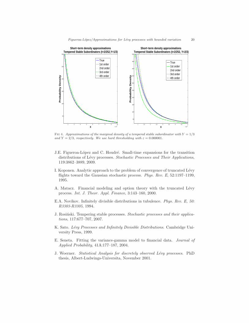
4.3. Tempered Stable Subordinators

Finally, we also consider the class of tempered stable subordinators introducedin Barndorff-Nielsen and Shephard (2002). Concretely, given a positive stablerandom variable Z with cumulant transformation log E e−uZ = −δ(2u)Y , atempered stable random variable X has probability density

p(x;Y, δ, γ) = eδγp(x;Y, δ)e−1

2γ1/Y x,


where p(x;Y, δ) is the probability density Z. It can be shown that X is aninfinitely divisible random variable with Levy density of the form:

s(x) = δ2YY

Γ(1− Y )x−1−Y e−

1

2γ1/Y x1{x>0}.

Note that this process is a tempered stable process as described in Introduction.One motivation of working with this process is that its probability density enjoysa series expansion of the form:

p(x;Y, δ, γ) = eδγe−1

2γ1/Y x 1

2π

∞∑

j=1

(−1)j−1 sin(jY π)Γ(jY + 1)

j!δj2jY+1x−jY −1.

A tempered stable subordinator is a subordinator whose time t = 1 densityis p(·;Y, δ, γ). Note in particular that Xt has probability density p(·;Y, δt, γ).Figure 4 shows the polynomial approximations pt(x) using the “hard” densityapproximation sε = s(x)1|x|≥ε for the value setting

γ = 1, δ = 1, t = 2/252,

and the values of Y = 1/3 and Y = 2/3. Note that for Y = 1/3 there is notmuch difference for order approximations greater than 2; however, for Y = 2/3,we note that upper order approximations significantly improve the plain firstorder approximation.

−0.01 −0.005 0 0.005 0.010

10

20

30

40

50

60

70

80

90

100

x = Log Return in 1 day (1/365 y.)

Pro

ba

bili

ty D

en

sity

Short−term density approximationsVariance Gamma Process

True1st5th11th17th23rd29th35thStnd 35th

−1 −0.8 −0.6 −0.4 −0.2 0 0.2 0.4 0.6 0.8 1

x 10−3

0

100

200

300

400

500

600

700

800

x= Log Return in 1/3 of a Day (1/(365*3) y.)

Pro

ba

bili

ty D

en

sity

Short−term density approximationsVariance Gamma Process

True1st5th11th17th23rdStnd 23rd

Fig 1. Approximations of the marginal density of a VG model with t = 1

365years and t =

1

3∗365years using the approximation s(x)1|x|≥ε with ε = .0001 and ε = .000001, respectively.

Acknowledgments: This research was partially supported by the NSF grant #DMS 0906919. The author is grateful to an anonymous referee for constructivesuggestions for improving the paper.


−0.04 −0.03 −0.02 −0.01 0 0.01 0.02 0.03 0.040

5

10

15

20

25

30

35

40

Hard short−term density approximationsCGMY model (C=280, G=M=102, Y=.1191)

x =Log Return in 1 day (1/365 y)

Pro

ba

bili

ty D

en

sity

True (FFT)1st5th11th17th23rd29th35th41st47thStd 47th

−0.04 −0.03 −0.02 −0.01 0 0.01 0.02 0.03 0.040

5

10

15

20

25

30

35

40

Smooth short−term density approximationsCGMY model (C=280, G=M=102, Y=.1191)

x = Log return in 1 day (1/365 y)P

rob

ab

ility

De

nsity

True (FFT)1 st5th11th17th23rd29th35th41st47thStnd 47th

Fig 2. Approximations of the marginal density of a CGMY model with t = 1

365years using

the approximations s(x)1|x|≥ε with ε = .0002, and s(x)e−ε/|x| with ε = .0001, respectively.

References

O.E. Barndorff-Nielsen. Probability densities and Levy densities. TechnicalReport 18, Centre for Mathematical Physics and Stochastics (MaPhySto).Aarhus Univ., 2000.

O.E. Barndorff-Nielsen and F. Hubalek. Probability densities and Levy densi-ties. Technical Report 12, Thiele Research Report, Aarhus Univ., 2006.

O.E. Barndorff-Nielsen and F. Hubalek. Probability measures, Levy measures,and analyticity in time. Bernoulli, 3(14):764–790, 2008.

O.E. Barndorff-Nielsen and N. Shephard. Normal modified stable processes.Theory of Probability and Mathematical Statistics, 65: 1–19, 2002.

S.I. Boyarchenko and S.Z. Levendorskii. Option pricing for truncated Levyprocesses. International journal of theoretical and applied finance, 3:549–552,2000.

P. Carr, D. Madan, and E. Chang. The variance Gamma process and optionpricing. European Finance Review, 2:79–105, 1998.

P. Carr, H. Geman, D. Madan, and M. Yor. The fine structure of asset returns:An empirical investigation. Journal of Business, pages 305–332, April 2002.

R. Cont, J. Bouchaud, and M. Potters. Scaling in financial data: Stable lawsand beyond. in Scale Invariance and Beyond, Dubrulle, B., Graner, F., andSornette, D., eds., 1997.


−0.2 −0.15 −0.1 −0.05 0 0.05 0.1 0.15 0.20

1

2

3

4

5

6

7

8

9

10

x = Log Return in 1 day (1/252 y)

Pro

ba

bili

ty D

en

sity

Hard short−term density approximationsCGMY model (C=125, G=M=83, Y=0.8)

True (FFT)

1st

11th

23rd

35th

47th

59th

−0.1 −0.05 0 0.05 0.1 0.150

5

10

15


x = Log Return in 1/3 day (1/(3*252) y)

Pro

ba

bili

ty D

en

sity

True (FFT)1st11th23rd35th47th59th

−0.1 −0.08 −0.06 −0.04 −0.02 0 0.02 0.04 0.06 0.08 0.10

2

4

6

8

10

12

14

16

18

20



Pro

ba

bili

ty D

en

sity


−0.08 −0.06 −0.04 −0.02 0 0.02 0.04 0.06 0.080

5

10

15

20

25

30



Pro

ba

bili

ty D

en

sity


Fig 3. Approximations of the marginal density of a CGMY model for different values of tusing the approximations s(x)1|x|≥ε.


2 3 4 5 6 7 8 9 10

x 10−4

50

100

150

200

250

300

x

Pro

ba

bili

ty D

en

sity

Short−term density approximationsTempered Stable Subordinators (t=2/252,Y=1/3)

True1st order2nd order3rd order4th order

1 1.5 2 2.5 3 3.5 4 4.5 5

x 10−3

50

100

150

200

250

300

350

400

450

500

xP

rob

ab

ility

De

nsity

Short−term density approximationsTempered Stable Subordinators (t=2/252, Y=2/3)

True1st order2nd order3rd order4th order

Fig 4. Approximations of the marginal density of a tempered stable subordinator with Y = 1/3and Y = 2/3, respectively. We use hard thresholding with ε = 0.000001.

J.E. Figueroa-Lopez and C. Houdre. Small-time expansions for the transitiondistributions of Levy processes. Stochastic Processes and Their Applications,119:3862–3889, 2009.

I. Koponen. Analytic approach to the problem of convergence of truncated Levyflights toward the Gaussian stochastic process. Phys. Rev. E, 52:1197–1199,1995.

A. Matacz. Financial modeling and option theory with the truncated Levyprocess. Int. J. Theor. Appl. Finance, 3:143–160, 2000.

E.A. Novikov. Infinitely divisible distributions in tubulence. Phys. Rev. E, 50:R3303-R3305, 1994.

J. Rosinski. Tempering stable processes. Stochastic processes and their applica-tions, 117:677–707, 2007.

K. Sato. Levy Processes and Infinitely Divisible Distributions. Cambridge Uni-versity Press, 1999.

E. Seneta. Fitting the variance-gamma model to financial data. Journal ofApplied Probability, 41A:177–187, 2004.

J. Woerner. Statistical Analysis for discretely observed Levy processes. PhDthesis, Albert-Ludwings-Universita, November 2001.

Approximations for the distributions of bounded … for the distributions of bounded variation...

Documents

Transcript of Approximations for the distributions of bounded … for the distributions of bounded variation...