Approximation Theory (( תורתהקרוב

Hooke’s law: F(l)=k(l-E), where F(l) is the force required to stretch the spring l units, E is the length with no force applied, k is the spring constant.

F l

0 5.3

2 7.0

4 9.4

6 12.3

Discrete Data Approximation

xi yi

1 1.3

2 3.5

3 4.2

4 5.0

5 7.0

6 8.8

7 10.1

8 12.5

9 13.0

10 15.6

Discrete Data Approximation

Discrete Least Square Approximation

•A minimax problem: find a and b to minimize baxy ii

i

10,...,2,1

max

•Find a and b to minimize the absolute deviation

10

1iii baxy

•Find a and b to minimize the least square error

10

1

2

iii baxy

קירוב ע"י ריבועים פחותים

1x

nxxx ,..., 21

...

נתונים שמודדים בניסוי תמיד כוללים שגיאות מדידה ולכן אין סיבה שנקרבאת הנתונים ע"י פולינום אינטרפולציה שיעבור דרך הנקודות במדויק.

רצוי למצוא פולינום או פונקציה אחרת פשוטה שתעבור הכי קרוב לכל הנקודות. (Least Squareריבועים פחותים )השיטה שמאפשרת קירוב כזה היא שיטת

f(xiוערכי פונקציה ) נקודות nנניח כי נתונים

nx

xaapונניח שרוצים להעביר קו ישר 10

כך שיהיה קרוב לכל הנקודות )קו מגמה ליניארית(

Linear Regression

)()(נגדיר סכום השאריות בריבוע: ii xpxf

n

iiir xaaxfS

1

210 )]()([

יהיה מינימאלי; כלומר שהקו יהיה הכי קרוב לנקודות.Srנרצה שה-

Sr שיתנו את הקירוב הטוב ביותר ע"י גזירת a0 , a1נמצא את המקדמים

קו מגמה ליניארית

n

iiii

r

n

iii

r

xxaaxfa

S

xaaxfa

S

110

1

110

0

0])([2

0])([2

n

iii

n

ii

n

ii

n

ii

n

ii

xfxaxax

xfaxna

111

20

1

1110

)( )( )(

)( )(

n

iix

1 )(

)משוואות נורמאליות(: a0 , a1 משוואות ליניאריות ל 2מכאן נקבל מערכת של

יצטמצם 0a ונחסיר. האיבר עם nנכפיל משוואה ראשונה ב והשנייה ב- :1aונקבל

n

i

n

iii

n

i

n

i

n

iiiii

xnx

xfxnxfxa

1 1

22

1 1 11

)(

)()(

קו מגמה ליניארית )המשך( יהיו פשוטים יותר אם נסמן ממוצעיםa0 , a1הביטויים ל

221 )(

)()(

ii

iiii

xxn

xfxxfxna

n

iiin

n

iin

n

iin xfxxfxffxx

1

1

1

1

1

1 ... ),( ),( ,

a1ונציב אותם לנוסחת

ונקבל:

:a0נשתמש בתוצאה הזאת יחד אם המשוואה ה"נורמאלית" הראשונה לחישוב xafa 10

: דרוש לבנות קו המגמה לנתונים הבאים )שנמדדו בניסוי(:דוגמה ii yx

5.5 7

0.6 6

5.3 5

0.4 4

0.2 3

5.2 2

5.0 1

2 4 6 8x

1

2

3

4

5

6

y

4 20 24/7 17.07 ממוצע

49

36

25

16

9

4

1

2x

38.5

36

17.5

16

6

5

0.5 ii yx

0714.048393.0

8393.0420

407.17

724

0

27

24

1

a

a

22 xx

fxxf

Least Square Approximation

xi yi

1 1.3

2 3.5

3 4.2

4 5.0

5 7.0

6 8.8

7 10.1

8 12.5

9 13.0

10 15.6

Least Square Approximation

xi yi

1 1.3

2 3.5

3 4.2

4 5.0

5 7.0

6 8.8

7 10.1

8 12.5

9 13.0

10 15.6

? ?, ,)( babaxxP

Least Square Approximation: Example

36.05538510

4.5725581385

538.15538510

81554.57210

21

20

a

a

Least Square Approximation

xi yi

1 1.3

2 3.5

3 4.2

4 5.0

5 7.0

6 8.8

7 10.1

8 12.5

9 13.0

10 15.6

P)x(=1.538x-0.36

Least Square Approximation: P(x)=ax (Zero-Intercept)

n

iiir axxfS

1

2])([

n

iiii

r xaxxfa

S

10])([2

n

ii

n

iii

x

xfxa

1

2

1)(

axxP )(

Least Square Approximation: P(x)=ax (Zero-Intercept)

a)

F(l) l

2 7.0

4 9.4

6 12.3

k=?

? ,3.5 ),()( kEElklF

b) add

more data

F(l) l

3 8.3

5 11.3

8 14.4

10 15.9

k=?

Least Square Approximation: Example

??xy 9.07ˆ

xy 0.18ˆ i=1, 2, 3i=1, 2, 3::דרך דרך

?2 ie

איכות הקירובהאם הקירוב "טוב" או לא?

2 4 6 8x

1

2

3

4

5

y

2 4 6 8x

1

2

3

4

5

6

y

נגדיר

n

iit fxfS

1

)ונזכור ש (])([2

n

iir xaaxfS

1

210 )]()([

א)

ב(

נגדיר כ rואז מקדם המתאם )הקורלציה( t

rt

S

SSr

מקדם המתאם מכמת את החלק מפיזור הנתונים שניתן ליחס להתנהגות מסודרת לפי קו המגמה. שאר הפיזור נובע משגיאות אקראיות.

במקרה ב'0.18 במקרה א' ו- 0.93מקדם המתאם הוא

ליניאריזאציה של משוואות הקירוב

ערכי הפונקציה וידוע שהפונקציה מתנהגת כ- n נניח כי בניסוי נמדדו1(xbebxf 1

0)(

כך שהקירוב ע"י הפונקציה יהיה b1 ,b 0דרוש למצוא את המקדמים משני האגפים של המשוואה:lnהכי קרוב לנקודות המדידה. ניקח

xbbebxfaa

xb

10

1100 ln)ln()(ln

iiנסמן ונקבל משוואת קו המגמה yxf )(ln

ii xaay 10 ניתן למצוא לפי הנוסחאות של קו המגמה ואחר כךa1 ,a 0המקדמים

0לחשב .0

aeb

2 4 6 8x

123456

ln fx

1 2 3 4 5 6 7x

100

200

300

400fx

Least Square Approximation: Example

? ,? ?, ,)( 2 ebabexy ax

Least Square Approximation: Example

axbybexy ax lnln)(

122.15.7875.115

5.7422.14404.9875.11ln

5056.05.7875.115

404.95.7422.145

2

2

b

axexy 5056.0071.3)(

WHYWHY?? 0 ie

Least Square Approximation: Example (cont.)

xexy 5056.0071.3)(

ליניאריזאציה של משוואות הקירוב )המשך(נניח כי הפונקציה מתנהגת כ . גם במקרה הזה 2(

נשתמש בהתמרה לוגריתמית:

10)( cxcxf

xccxcxf

aa

c lnln)ln()(ln

10

1100

iiכמו במקרה הקודם נסמן ושוב נקבל משוואת קו המגמה yxf )(ln

ii aay 10 1: דרוש לקרב את הנתונים שבטבלה ע"י הפונקציה דוגמה

0)( cxcxf

4.85

7.54

4.33

7.12

5.01

424.3589.2128.2609.1

412.2921.1740.1386.1

345.1208.1224.1099.1

368.0480.0531.0693.0

00693.00 yfyxxfx 2lnln)(

510.1240.1986.0957.0

75.1

688.00

0

21

5.0)(

5.0

688.0957.0748.1986.0

748.1957.024.1

986.0957.051.1

xxf

ec

a

a

ליניאריזאציה של משוואות הקירוב )המשך(

נניח כי הפונקציה מתנהגת כ . 3(xd

xdxf

10)(

נבצע התמרה:

)(

1,,

1,

1

11

)(

1

0

11

00

1

0

ii xf

yd

da

xda

x

d

dxf

ושוב נקבל את משוואת קו המגמה

ii aay 10

נמצא לפי הנוסחאות של קו המגמה ואחר כך a1 ,a 0את המקדמים

נחשב

0

11

00 ,

1

a

ad

ad

קירוב ע"י פולינום בשיטת ריבועים פחותים

נניח כי נתונות הנקודות הבאות

2 3 4 5 6 7x

5101520253035

y

ורוצים להתאים עקומה שתעבורפרבולה!קרוב לנקודות.

nבאופן כללי נניח כי רוצים להתאים את הפולינום מדרגת n

nn xaxaaxp 10)(כך שהקירוב יהיה הטוב n<m) הנקודות הנמדדות )mלסדרת

שוב מגדירים: וכדי שהפולינום יהיה הכי ביותר.קרוב לנתונים דורשים:

m

iinir xpxfS

1

2)]()([

m

i

ni

ninii

n

r

m

ii

ninii

r

m

ii

ninii

r

xxaxaaxfa

S

xxaxaaxfa

S

xxaxaaxfa

S

110

1

110

1

1

010

0

0])([2

0])([2

0])([2

קירוב ע"י פולינום בשיטת ריבועים פחותים

m

i

ni

ninii

n

r

m

ii

ninii

r

m

ii

ninii

r

xxaxaaxfa

S

xxaxaaxfa

S

xxaxaaxfa

S

110

1

110

1

1

010

0

0])([2

0])([2

0])([2

מקדמים של הפולינום הם פתרון של מערכת משוואות:

m

i

m

i

kji

n

kk

jii

j

r njxaxxfa

S

1 10 ,...,1 ,0 ,02)(2

או

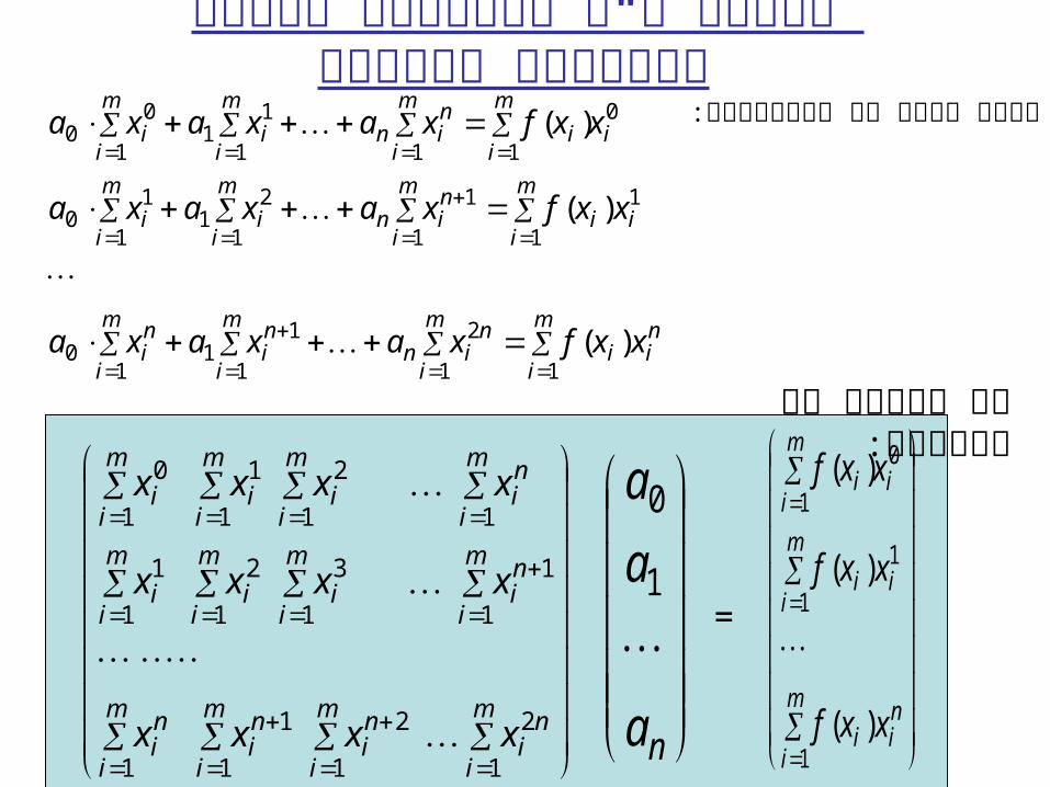
קירוב ע"י פולינום בשיטת ריבועים פחותים

m

i

nii

m

i

nin

m

i

ni

m

i

ni

m

iii

m

i

nin

m

ii

m

ii

i

m

ii

m

i

nin

m

ii

m

ii

xxfxaxaxa

xxfxaxaxa

xxfxaxaxa

11

2

1

11

10

1

1

1

1

1

21

1

10

0

111

11

1

00

)(

)(

)(

ניתן לסדר את המשוואות:

m

i

ni

m

i

ni

m

i

ni

m

i

ni

m

i

ni

m

ii

m

ii

m

ii

m

i

ni

m

ii

m

ii

m

ii

xxxx

xxxx

xxxx

1

2

1

2

1

1

1

1

1

1

3

1

2

1

1

11

2

1

1

1

0

או בצורה של מטריצה:

na

a

a

1

0

m

i

nii

m

iii

i

m

ii

xxf

xxf

xxf

1

1

1

0

1

)(

)(

)(

=

קירוב ע"י פולינום בשיטת ריבועים פחותים: דוגמא

m

i

nii

m

i

nin

m

i

ni

m

i

ni

m

iii

m

i

nin

m

ii

m

ii

i

m

ii

m

i

nin

m

ii

m

ii

xxfxaxaxa

xxfxaxaxa

xxfxaxaxa

11

2

1

11

10

1

1

1

1

1

21

1

10

0

111

11

1

00

)(

)(

)(

4015.43828.15625.1875.1

4514.55625.1875.1 5.2

7680.8875.1 5.2 5

210

210

210

aaa

aaa

aaa

22102 )( xaxaaxP

?

?

?

2

1

0

a

a

a

5

1

22

2 ?)(i

ii xPye

קירוב ע"י פולינום בשיטת ריבועים פחותים: דוגמא

4015.43828.15625.1875.1

4514.55625.1875.1 5.2

7680.8875.1 5.2 5

210

210

210

aaa

aaa

aaa

22 8437.08641.00052.1)( xxxP

8437.0 ,8641.0 ,0052.1 210 aaa

5

1

422

2 1076.2)(i

ii xPye

Least Square Approximation: Exam-1

i 1 2 3 4 5 6 7 8 9 10

xi 4.0 4.2 4.5 4.7 5.1 5.5 5.9 6.3 6.8 7.1

yi 102.56 113.18 130.11 142.05 167.53 195.14 224.87 256.73 299.50 326.72

a. Construct the LS polynomial of degree one and compute the error.

b. Construct the LS polynomial of degree two and compute the error.

c. Construct the LS polynomial of degree three and compute the error.

d. Construct the LS approximation of the form and compute the error.

e. Construct the LS approximation of the form and compute the error.

f. What form of the relationship is the best fit for the data?

axbeabx