Approximating Multisector New Keynesian Models —

Extended Version∗

Carlos Carvalho

Central Bank of Brazil

PUC-Rio

Fernanda Nechio

Federal Reserve Bank of San Francisco

November, 2017

Abstract

A calibrated three-sector model with a suitably chosen distribution of price stickiness

can closely approximate the dynamic properties of New Keynesian models with a much

larger number of sectors. The parameters of the approximate three-sector distribution are

such that both the approximate and the original distributions share the same (i) average

frequency of price changes, (ii) cross-sectional average of durations of price spells, (iii)

cross-sectional standard deviation of durations of price spells, (iv) cross-sectional skewness

of durations of price spells, and (v) cross-sectional kurtosis of durations of price spells.

This result should prove useful to the literature that takes into account heterogeneity in

price stickiness in DSGE models. In particular, it should allow for the estimation of such

models at a much reduced computational cost.

JEL classification codes: E22, J6, E12

Keywords: multisector approximation, heterogeneity, factor specificity

∗For comments and suggestions we thank an anonymous referee. In this supplement to our main paper weprovide several extensions of the model and results. The views expressed in this paper are those of the authorsand do not necessarily reflect the position of the Federal Reserve Bank of San Francisco, the Federal ReserveSystem or the Central Bank of Brazil. E-mails: cvianac@econ.puc-rio.br and fernanda.nechio@sf.frb.org.

1

1 Introduction

The macroeconomics literature has provided substantial evidence of significant heterogeneity in

the average frequencies with which firms in different sectors of the economy change their prices,

both in the U.S. and in other countries (e.g., Blinder et al., 1998, Bils and Klenow, 2004,

Nakamura and Steinsson, 2008, and Klenow and Malin, 2011 for the U.S. economy; Dhyne

et al., 2006, and references cited therein for the euro area).

The literature has also shown that accounting for this heterogeneity matters for the dynamic

properties of New Keynesian economies (e.g., Carvalho, 2006, Nakamura and Steinsson, 2010,

Carvalho and Nechio, 2011 and Pasten, Schoenle and Weber, 2016). Models that allow for het-

erogeneity in frequency of price adjustments yield substantially different dynamics for aggregate

variables than models that assume that firms adjust prices at a common (average) frequency.

In response to monetary shocks, for example, heterogeneous multisector models feature much

larger and more persistent real effects than one-sector economies with similar average degrees of

nominal rigidities. Heterogeneity in price stickiness also has implications for optimal monetary

policy (e.g., Aoki, 2001 and Eusepi, Hobijn and Tambalotti, 2011).1

Working with large-scale multisector models, however, is computationally costly. As a

consequence, while one can find several calibrated multisector models in the literature, the set

of papers that entertain estimating such large-scale models is much more limited (exceptions

include, for example, Carvalho and Lee, 2011 and Bouakez, Cardia and Ruge-Murcia, 2009).

In this paper we show how a large-dimension multisector economy can be approximated by a

three-sector model that, aside from the number of sectors, features the same model ingredients

as the original economy. In particular, we show that for a suitably chosen distribution of price

stickiness, aggregate variables in the three-sector model feature similar dynamics than the

corresponding variables in the original model. A comparison of the impulse response functions

(IRFs) of the main aggregate variables in response to monetary and technology shocks shows

that the three-sector economy follows the dynamic properties of the original (larger-scale) model

extremely closely.

The empirical evidence shows that the distribution of price stickiness is highly asymmetric,

and with a long right tail. Therefore, there is a larger mass of sectors adjusting more frequently

and a smaller mass adjusting very infrequently. These features are well summarized by five

moments of the distribution, namely; (i) average frequency of price changes, (ii) cross-sectional

1These papers also study the effects of sector-specific shocks. Because our approximation strategy entailsconstructing an artificial three-sector economy with price stickiness distribution that matches moments of thelarger (original) distribution, there is no direct mapping between sectors in the original and approximatedeconomies. Hence our focus on aggregate shocks.

2

average of durations of price spells, (iii) cross-sectional standard deviation of durations of price

spells, (iv) the cross-sectional skewness of durations of price spells, and (v) cross-sectional

kurtosis of durations of price spells.

Our approximation strategy entails constructing an artificial small-scale distribution of price

rigidity that matches the same shape features of the original one. More specifically, given these

five moments of the original distribution of price stickiness, we build a three-sector distribution

by choosing sectoral weights and price adjustment frequencies such that both the approximate

and the original distributions share the same aforementioned five moments.

We apply our approximation to the U.S. distribution of price stickiness derived from Naka-

mura and Steinsson (2008), as well as to artificially-generated arbitrary distributions of price

rigidity. We test the performance of our approximation using the dynamic stochastic general

equilibrium (DSGE) model presented in Carvalho and Nechio (2016). The model features a

multisector economy where heterogeneity in the frequency of price adjustment is the key source

of heterogeneity.

The results show that our approximation performs extremely well. In particular, three-sector

economies parameterized with distributions of price stickiness that match the five aforemen-

tioned moments yield IRFs to monetary and technology shocks that are very close to the ones

obtained in the original economies. These results hold for approximations based on both the

U.S. distribution and on the artificially-generated arbitrary distributions of price rigidity.

2 A three-sector approximation

These features of the distributions of price stickiness are important in determining the dynamics

of aggregate variables in New Keynesian models (e.g., Carvalho, 2006, Nakamura and Steins-

son, 2010, and Carvalho and Nechio, 2011). In addition, Carvalho and Schwartzman (2015)

show that, under some conditions, moments of the distribution of price stickiness are sufficient

statistics for the real effects of nominal shocks.

Therefore, in order to approximate larger-scale economies with smaller-scale ones, one should

construct an artificial distribution of price stickiness that mimics the properties of the original

distribution. Given the empirical evidence on the skewness and the long tail of the original

distribution, this implies that both the approximate and the original distributions should exhibit

similar high-order moments.

To that end, we calculate the following moments of the original distribution of price sticki-

ness:

(i) Average frequency of price changes:

3

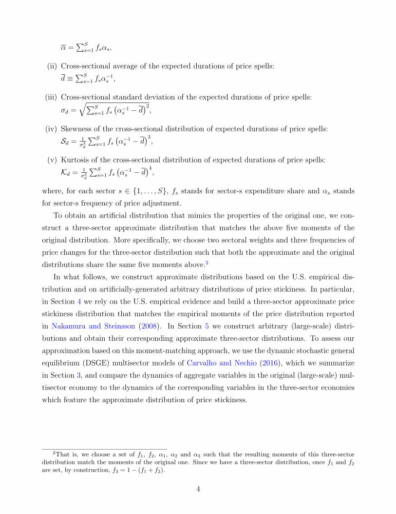
α =∑S

s=1 fsαs,

(ii) Cross-sectional average of the expected durations of price spells:

d ≡∑S

s=1 fsα−1s ,

(iii) Cross-sectional standard deviation of the expected durations of price spells:

σd =

√∑Ss=1 fs

(α−1s − d

)2,

(iv) Skewness of the cross-sectional distribution of expected durations of price spells:

Sd = 1σ3d

∑Ss=1 fs

(α−1s − d

)3,

(v) Kurtosis of the cross-sectional distribution of expected durations of price spells:

Kd = 1σ4d

∑Ss=1 fs

(α−1s − d

)4,

where, for each sector s ∈ {1, . . . , S}, fs stands for sector-s expenditure share and αs stands

for sector-s frequency of price adjustment.

To obtain an artificial distribution that mimics the properties of the original one, we con-

struct a three-sector approximate distribution that matches the above five moments of the

original distribution. More specifically, we choose two sectoral weights and three frequencies of

price changes for the three-sector distribution such that both the approximate and the original

distributions share the same five moments above.2

In what follows, we construct approximate distributions based on the U.S. empirical dis-

tribution and on artificially-generated arbitrary distributions of price stickiness. In particular,

in Section 4 we rely on the U.S. empirical evidence and build a three-sector approximate price

stickiness distribution that matches the empirical moments of the price distribution reported

in Nakamura and Steinsson (2008). In Section 5 we construct arbitrary (large-scale) distri-

butions and obtain their corresponding approximate three-sector distributions. To assess our

approximation based on this moment-matching approach, we use the dynamic stochastic general

equilibrium (DSGE) multisector models of Carvalho and Nechio (2016), which we summarize

in Section 3, and compare the dynamics of aggregate variables in the original (large-scale) mul-

tisector economy to the dynamics of the corresponding variables in the three-sector economies

which feature the approximate distribution of price stickiness.

2That is, we choose a set of f1, f2, α1, α2 and α3 such that the resulting moments of this three-sectordistribution match the moments of the original one. Since we have a three-sector distribution, once f1 and f2are set, by construction, f3 = 1− (f1 + f2).

4

3 Three New Keynesian models of factor specificity

Carvalho and Nechio (2016) present three versions of multisector DSGE models. In all three

models, identical infinitely-lived consumers supply labor and capital to intermediate firms that

they own, invest in a complete set of state-contingent financial claims, and consume a final

good. The latter is produced by competitive firms that bundle varieties of intermediate goods.

The monopolistically competitive intermediate firms that produce these varieties are divided

into sectors that only differ in their frequency of price changes. Labor and capital are the only

inputs in the production of intermediate goods.

The models differ, however, on their assumptions about the mobility of factor inputs across

sectors. In their benchmark model, they assume that capital and labor can be reallocated freely

across firms in the same sector but cannot move across sectors, i.e., factors are sector-specific.

The authors also entertain versions of their model in which factors are firm-specific, i.e., cannot

move across sectors nor firms within sectors; and factors are economy-wide and can move freely

across firms and sectors.

In the following, we provide some key ingredients of all three versions of Carvalho and Nechio

(2016) models, and refer the reader to the paper for detailed descriptions.

3.1 Sector-specific factors

The representative consumer maximizes:

E0

∞∑t=0

βt

(C1−σt − 1

1− σ−

S∑s=1

ωsN1+γs,t

1 + γ

),

subject to the flow budget constraint:

PtCt + PtIt + Et [Θt,t+1Bt+1] ≤S∑s=1

Ws,tNs,t +Bt + Tt +S∑s=1

Zs,tKs,t,

the law of motion for the stocks of sector-specific capital:

Ks,t+1 = (1− δ)Ks,t + Φ (Is,t, Ks,t) Is,t, ∀ s

Φ (Is,t, Ks,t) = Φ

(Is,tKs,t

)= 1− 1

2κ

(Is,tKs,t− δ)2

Is,tKs,t

,

Is,t ≥ 0,∀s

5

and a standard “no-Ponzi” condition. Et denotes the time-t expectations operator, Ct is con-

sumption of the final good, Ns,t denotes total labor supplied to firms in sector s, Ws,t is the

associated nominal wage rate, and ωs is the relative disutility of supplying labor to sector s.

Is,t denotes investment in sector-s capital, It ≡∑S

s=1 Is,t, Ks,t is capital supplied to firms in

sector s, and Zs,t is the associated nominal return on capital.

The final good can be used for either investment or consumption, and sells at the nominal

price Pt. Bt+1 accounts for the state-contingent value of the portfolio of financial securities

held by the consumer at the beginning of t + 1. Under complete financial markets, agents

can choose the value of Bt+1 for each possible state of the world at all times, subject to the

no-Ponzi condition and the budget constraint. Tt stands for profits received from intermediate

firms. The absence of arbitrage implies the existence of a nominal stochastic discount factor

Θt,t+1 that prices in period t any financial asset portfolio with state-contingent payoff Bt+1 at the

beginning of period t+1.3 β is the time-discount factor, σ−1 denotes the intertemporal elasticity

of substitution, γ−1 is the Frisch elasticity of labor supply, δ is the rate of depreciation. Finally,

the adjustment-cost function, Φ (.), is specified as in Chari, Kehoe and Mcgrattan (2000), where

Φ is convex and satisfies Φ (δ) = 1, Φ′ (δ) = 0, and Φ′′ (δ) = −κδ.

A representative competitive firm produces the final good, which is a composite of varieties

of intermediate goods. Monopolistically competitive firms produce such varieties. These firms

are divided into sectors indexed by s ∈ {1, ..., S}, each featuring a continuum of firms. Sectors

differ in the degree of price rigidity, as we detail below. Overall, firms are indexed by their

sector s, and are further indexed by j ∈ [0, 1]. The distribution of firms across sectors is given

by sectoral weights fs > 0, with∑S

s=1 fs = 1.

The final good is used for both consumption and investment by combining the intermediate

varieties. More specifically, the representative final-good-producing firm solves:

max PtYt −∑S

s=1fs

∫ 1

0

Ps,j,tYs,j,tdj

s.t. Yt =

(∑S

s=1f

1ηs Y

η−1η

s,t

) ηη−1

Ys,t =

(fθ−1θ

s

∫ 1

0

Yθ−1θ

s,j,t dj

) θθ−1

,

where Yt is the final good, Ys,t is the aggregation of sector-s intermediate goods, and Ys,j,t is

the variety produced by firm j in sector s. The parameters η ≥ 0, and θ > 1 are, respectively,

the elasticity of substitution across sectors and the elasticity of substitution within sectors. Pt

3 To avoid cluttering the notation, we omit explicit reference to the different states of nature.

6

is the price of the final good, Ps,t is the price index of sector-s intermediate goods, and Ps,j,t is

the price charged by firm j from sector s.

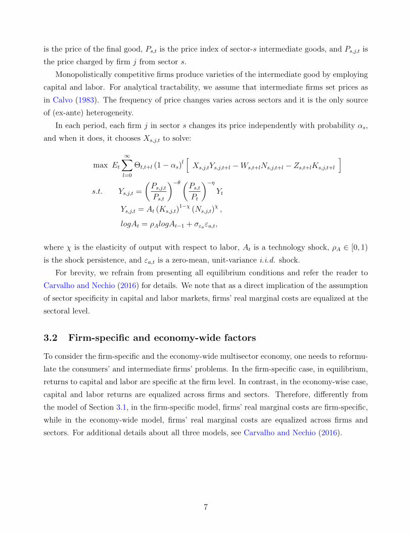
Monopolistically competitive firms produce varieties of the intermediate good by employing

capital and labor. For analytical tractability, we assume that intermediate firms set prices as

in Calvo (1983). The frequency of price changes varies across sectors and it is the only source

of (ex-ante) heterogeneity.

In each period, each firm j in sector s changes its price independently with probability αs,

and when it does, it chooses Xs,j,t to solve:

max Et

∞∑l=0

Θt,t+l (1− αs)l[Xs,j,tYs,j,t+l −Ws,t+lNs,j,t+l − Zs,t+lKs,j,t+l

]s.t. Ys,j,t =

(Ps,j,tPs,t

)−θ (Ps,tPt

)−ηYt

Ys,j,t = At (Ks,j,t)1−χ (Ns,j,t)

χ ,

logAt = ρAlogAt−1 + σεaεa,t,

where χ is the elasticity of output with respect to labor, At is a technology shock, ρA ∈ [0, 1)

is the shock persistence, and εa,t is a zero-mean, unit-variance i.i.d. shock.

For brevity, we refrain from presenting all equilibrium conditions and refer the reader to

Carvalho and Nechio (2016) for details. We note that as a direct implication of the assumption

of sector specificity in capital and labor markets, firms’ real marginal costs are equalized at the

sectoral level.

3.2 Firm-specific and economy-wide factors

To consider the firm-specific and the economy-wide multisector economy, one needs to reformu-

late the consumers’ and intermediate firms’ problems. In the firm-specific case, in equilibrium,

returns to capital and labor are specific at the firm level. In contrast, in the economy-wise case,

capital and labor returns are equalized across firms and sectors. Therefore, differently from

the model of Section 3.1, in the firm-specific model, firms’ real marginal costs are firm-specific,

while in the economy-wide model, firms’ real marginal costs are equalized across firms and

sectors. For additional details about all three models, see Carvalho and Nechio (2016).

7

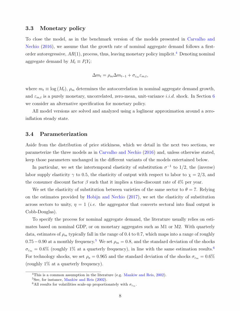
3.3 Monetary policy

To close the model, as in the benchmark version of the models presented in Carvalho and

Nechio (2016), we assume that the growth rate of nominal aggregate demand follows a first-

order autoregressive, AR(1), process, thus, leaving monetary policy implicit.4 Denoting nominal

aggregate demand by Mt ≡ PtYt:

∆mt = ρm∆mt−1 + σεmεm,t,

where mt ≡ log (Mt), ρm determines the autocorrelation in nominal aggregate demand growth,

and εm,t is a purely monetary, uncorrelated, zero-mean, unit-variance i.i.d. shock. In Section 6

we consider an alternative specification for monetary policy.

All model versions are solved and analyzed using a loglinear approximation around a zero-

inflation steady state.

3.4 Parameterization

Aside from the distribution of price stickiness, which we detail in the next two sections, we

parameterize the three models as in Carvalho and Nechio (2016) and, unless otherwise stated,

keep those parameters unchanged in the different variants of the models entertained below.

In particular, we set the intertemporal elasticity of substitution σ−1 to 1/2, the (inverse)

labor supply elasticity γ to 0.5, the elasticity of output with respect to labor to χ = 2/3, and

the consumer discount factor β such that it implies a time-discount rate of 4% per year.

We set the elasticity of substitution between varieties of the same sector to θ = 7. Relying

on the estimates provided by Hobijn and Nechio (2017), we set the elasticity of substitution

across sectors to unity, η = 1 (i.e. the aggregator that converts sectoral into final output is

Cobb-Douglas).

To specify the process for nominal aggregate demand, the literature usually relies on esti-

mates based on nominal GDP, or on monetary aggregates such as M1 or M2. With quarterly

data, estimates of ρm typically fall in the range of 0.4 to 0.7, which maps into a range of roughly

0.75−0.90 at a monthly frequency.5 We set ρm = 0.8, and the standard deviation of the shocks

σεm = 0.6% (roughly 1% at a quarterly frequency), in line with the same estimation results.6

For technology shocks, we set ρa = 0.965 and the standard deviation of the shocks σεm = 0.6%

(roughly 1% at a quarterly frequency).

4This is a common assumption in the literature (e.g. Mankiw and Reis, 2002).5See, for instance, Mankiw and Reis (2002).6All results for volatilities scale-up proportionately with σεm .

8

Finally, we calibrate investment adjustment costs, κ, such that each model roughly matches

the standard deviation of investment relative to the standard deviation of GDP in the data. For

that, we consider monetary and technology shocks one at a time. When analyzing the response

to monetary shocks, we set κ to 40, while when analyzing the response to technology shocks, we

set κ to 15. The remaining parameter values are unchanged from the baseline parameterization

when considering one or the other shock.

To be able to assess our approximation approach, it remains to specify the original dis-

tributions of price stickiness to be approximated. In what follows, we construct approximate

distributions based on the U.S. empirical distribution in Sections 4, and based on artificially-

generated arbitrary distributions of price stickiness in Section 5.

4 Approximating the U.S. empirical distribution

In this section we resort to the available microeconomic evidence on price rigidity in the U.S.

to pin down the distribution of price rigidity across sectors.

In particular, we use the statistics on the frequency of regular price changes — those that

are not due to sales or product substitutions — reported by Nakamura and Steinsson (2008).

More specifically, the U.S. distribution of price stickiness we consider consists of weights and

frequencies of price changes for 67 expenditure classes of goods and services.7 In the model,

each class is identified with a sector.

Following the approach described in Section 2, we construct a three-sector approximate

distribution. The original and the artificial distributions are such that the average frequency

of price changes equals 0.2 (which implies prices changing, on average, once every 4.7 months),

the cross-sectional average of durations of price spells equals 11.9 months, the cross-sectional

standard deviation of durations of price spells equals 9.3 months, the cross-sectional skewness

of durations of price spells equals 0.7 months, and the cross-sectional kurtosis of durations of

price spells equals 2.5 months

Figure 1 shows the impulse response functions (IRFs) to a monetary shock for the three

7Note that we aggregate the original 272 categories from Nakamura and Steinsson (2008) up into theircorresponding 67 expenditure classes of goods and services. To do so, we discard the category “Girls’ Outerwear,”for which the reported frequency of regular price changes is zero, aggregate up based on the 67 expenditureclasses, and renormalize the expenditure weights to sum to unity. The frequency of price changes for eachexpenditure class is obtained as the weighted average of the frequencies for the underlying categories, using theexpenditure weights provided by Nakamura and Steinsson (2008). Expenditure-class weights are given by thesum of the expenditure weights for those categories. As an example of what this aggregation entails, the resulting“New and Used Motor Vehicles” class consists of the categories “Subcompact Cars”, “New Motorcycles”, “UsedCars”, “Vehicle Leasing” and “Automobile Rental”; the “Fresh Fruits” class comprises four categories: “Apples”,“Bananas”, “Oranges, Mandarins etc.” and “Other Fresh Fruits.”

9

models; economy-wide, sector-, and firm-specific factor markets. For brevity, the figure only

reports the IRFs for real GDP and inflation. The approximation for other variables are provided

in the Appendix Figures A1 to A3.8

Figure 1: Impulse response functions in the 67-sector and the approximate three-sectoreconomies to a monetary shock.

The panels show that for all three models, the three-sector model calibrated with the ap-

proximate distribution does a great job in replicating the impulse response functions of output

8Note that we aggregate the original 272 categories from Nakamura and Steinsson (2008) up into their corre-sponding 67 expenditure classes of goods and services. Approximating directly from the 271-sector distributionfrom Nakamura and Steinsson (2008) yields similar results, as reported in the Appendix Figures A7 and A8.

10

and inflation (and similarly for the other aggregate variables in the model). The largest ap-

proximation error is attained at the firm-specific model and equals 0.0006.

Figure 2 shows the impulse response functions of GDP and inflation to a technology shock

for the same three models. Results are qualitatively similar. For all model versions, the three-

sector model calibrated with the approximate distribution tracks very closely the dynamics of

the impulse response functions of output and inflation in the original 67-sector models. The

approximation for other variables are provided in the Appendix Figures A4 to A6.

Figure 2: Impulse response functions in the 67-sector and the approximate three-sectoreconomies to a technology shock.

11

5 Approximating arbitrary distributions

The results above are based on an approximate three-sector distribution obtained from the U.S.

empirical evidence. In this section we consider our approximation from artificially-generated

distributions of price stickiness. To that end, we construct 67-sector distributions in which both

the frequency of price adjustment and the sectoral weight are chosen arbitrarily. In particular,

we start by constructing a vector of frequencies of price changes that ranges from 0.999 to

0.008, declining in equal steps. Therefore, in this artificial 67-sector distribution, price changes

range from, on average, once a month, in the most flexible sector, to once every 120 months,

in the stickiest sector. Next, we associate a set of arbitrary sectoral weights to this vector of

frequencies. More specifically, we generate sectoral weights from a Beta distribution in which

both shape parameters range from 0.5 to 10, in incremental steps of 0.25. This combination of

shape parameters yields a set of 1521 arbitrary vectors of sectoral weights. Finally, each vector

of weights is paired with the arbitrary vector of frequencies of price changes. This pairing yields

1521 sets of 67-sector price stickiness distributions.9

We, then, turn to the approximation for each of these arbitrary distributions. For that, we

follow the same steps as in Section 4. More specifically, for each arbitrary (67-sector) distribu-

tion, we calculate the five empirical moments described in Section 2 and obtain its corresponding

approximate three-sector distribution. Next, we parameterize the models of Section 3 under

the original and its approximate arbitrary distribution, and compare the responses to monetary

and technology shocks under the two parameterizations.

The exercise described above yields 1521 original and approximate parameterizations of

the three DSGE economies of Section 3. While we could, in principle, compare how each

approximation performs for each economic variable over time (in analogy to Figures 1 and

2), we, instead, report a summary of our results. In particular, for each model, variable and

approximation, we calculate the sum over time of the difference between the response of the

67-sector and the approximate three-sector models. This yields a distribution of the cumulative

approximation errors for each aggregate variable in the different models.

Figures 3 and 4 report the main results. They show the histograms of the cumulative

approximation errors for real GDP and inflation for the three models in response to a monetary

and technology shock, respectively. Both Figures show that, for all three models of factor

specificity, the three-sector approximation performs extremely well. In all cases, the cumulative

approximation error across all arbitrary price stickiness distributions is in the order of 10−3 to

10−2. The Appendix Figures A9 to A14 confirm that these results also hold for the other main

9Note that all distributions have the same vector of price stickiness but vary in the set of sectoral weights.

12

aggregate variables in the models.

Figure 3: Distribution of the cumulative approximation errors in response to a monetaryshock.

6 Robustness

To test for the robustness of our results, in this section we consider an alternative distribution

of price stickiness and variations to the models’ specifications.

In particular, we start by performing our approximation approach on the price stickiness

distribution from Bils and Klenow (2004). We follow the same steps as described in Sections

2 and 4 and construct a three-sector distribution of price stickiness that features the same

five moments (described in Section 2) as the original distribution of 350-categories from Bils

13

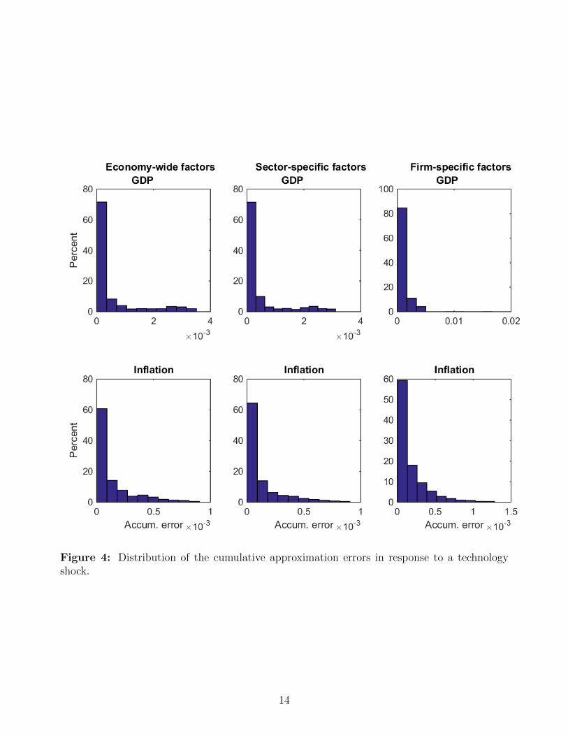
Figure 4: Distribution of the cumulative approximation errors in response to a technologyshock.

14

and Klenow (2004). In particular, the original and the artificial distributions are such that

the average frequency of price changes equals 0.3 (which implies prices changing, on average,

once every 3.8 months), the cross-sectional average of durations of price spells equals 7 months,

the cross-sectional standard deviation of durations of price spells equals 7.8 months, the cross-

sectional skewness of durations of price spells equals 4.1 months, and the cross-sectional kurtosis

of durations of price spells equals 36.9 months. Results, reported in Figure 5, confirm that our

approximation approach performs really well.

Figure 5: Impulse response functions in the 350-sector and the approximate three-sectoreconomies: monetary shock.

Next, we consider alternative model specifications. More specifically, we assume that mon-

15

etary policy is conducted according to an interest rate rule subject to persistent shocks:

IRt = β−1(

PtPt−1

)φπ ( GDPtGDP n

t

)φyεv,t,

where IRt is the short-term nominal interest rate, GDPt is gross domestic product, GDP nt

denotes gross domestic product when all prices are flexible, φπ and φy are the parameters

associated with Taylor-type interest-rate rules. εv,t is a persistent shock with process εv,t =

ρvεv,t−1 + σεvεv,t, where εv,t is a zero-mean, unit-variance i.i.d. shock, and ρv ∈ [0, 1).

To calibrate the version of the model with the above interest rate rule, we set φπ = 1.5,

φy = 0.5/12, and ρv = 0.965, and set the investment cost parameter κ to 45, which roughly

implies that the model matches the standard deviation of investment in the data relative to the

standard deviation of GDP. The remaining parameter values are unchanged from the baseline

specification.

We, then, follow the same steps as described in Sections 4 and 5, and assess our approxi-

mation using the U.S. empirical distribution of price stickiness and the set of arbitrary distri-

butions, respectively.

Figure 6 shows the impulse response functions of GDP and inflation to an expansionary

monetary shock for the three models of Section 3. Figure 7 reports the distribution of the

cumulative approximation errors obtained when the three models are calibrated using the arbi-

trary distributions described in Section 5.10 The approximation in the DSGE models assuming

an interest rule is quite accurate, with the three-sector approximate economy following closely

the dynamics of the original one. Figure 7 reinforces our conclusions.

Finally, we also entertain a version of the three models in which we assume a labor-only

economy by excluding capital accumulation, and a version in which we modify the Taylor rule

to allow for policy inertia. In all cases, our results are qualitatively unchanged and are available

upon request.

7 Conclusion

Our results show that a calibrated model with a suitably chosen three-sector distribution of price

stickiness can closely approximate the dynamic properties of New Keynesian models calibrated

with a much larger distribution. In particular, the set of sectoral weights and frequencies

of price adjustment in the approximate distribution are such that the latter and the original

distributions share the same (i) average frequency of price changes, (ii) cross-sectional average

10The approximation for all other variables are provided in the Appendix Figures A15 to A20.

16

Figure 6: Impulse response functions in the 67-sector and the approximate three-sectoreconomies: interest rate rule.

17

Figure 7: Distribution of the cumulative approximation errors in response to a monetaryshock: interest rate rule.

18

of durations of price spells, (iii) cross-sectional standard deviation of durations of price spells,

(iv) cross-sectional skewness of durations of price spells, and (v) cross-sectional kurtosis of

durations of price spells of the original distribution of price stickiness. Under those conditions,

we show that, for alternative multisector models with different assumptions for factor inputs

mobility, type of shocks and monetary policy specifications, the original and the approximate

distributions yield impulse response functions that are remarkably close. This result should

prove useful to the literature that takes into account heterogeneity of price stickiness in DSGE

models. In particular, it should allow for the estimation of such models at a much reduced

computational cost.

References

Aoki, Kosuke. 2001. “Optimal monetary policy responses to relative-price changes.” Journal

of Monetary Economics, 48(1): 55 – 80.

Bils, Mark, and Peter J. Klenow. 2004. “Some Evidence on the Importance of Sticky

Prices.” Journal of Political Economy, 112(5): 947–985.

Blinder, Alan S., Elie R. D. Canetti, David E. Lebow, and Jeremy B. Rudd. 1998.

Asking About Prices: A New Approach to Understanding Price Stickiness. Russell Sage Foun-

dation.

Bouakez, Hafedh, Emanuela Cardia, and Francisco Ruge-Murcia. 2009. “The Trans-

mission of Monetary Policy in a Multi-sector Economy.” International Economic Review,

50: 1243–1266.

Calvo, Guillermo. 1983. “Staggered Prices in a Utility Maximizing Framework.” Journal of

Monetary Economics, 12: 383–398.

Carvalho, Carlos. 2006. “Heterogeneity in Price Stickiness and the Real Effects of Monetary

Shocks.” Frontiers of Macroeconomics, 2(1): 1–58.

Carvalho, Carlos, and Felipe Schwartzman. 2015. “Selection and monetary non-neutrality

in time-dependent pricing models.” Journal of Monetary Economics, 76: 141 – 156.

Carvalho, Carlos, and Fernanda Nechio. 2011. “Aggregation and the PPP Puzzle in a

Sticky-Price Model.” The American Economic Review, 101(6): pp. 2391–2424.

19

Carvalho, Carlos, and Fernanda Nechio. 2016. “Factor specificity and real rigidities.”

Review of Economic Dynamics, 22: 208 – 222.

Carvalho, Carlos, and Jae Won Lee. 2011. “Sectoral price facts in a sticky-price model.”

Federal Reserve Bank of New York Staff Reports 495.

Chari, V. V., Patrick J. Kehoe, and Ellen R. Mcgrattan. 2000. “Sticky Price Models

of the Business Cycle: Can the Contract Multiplier Solve the Persistence Problem?” Econo-

metrica, 68(5): 1151–1179.

Dhyne, Emmanuel, Luis J. Alvarez, Herve Le Bihan, Giovanni Veronese, Daniel

Dias, Johannes Hoffmann, Nicole Jonker, Patrick Lunnemann, Fabio Rumler, and

Jouko Vilmunen. 2006. “Price Changes in the Euro Area and the United States: Some Facts

from Individual Consumer Price Data.” Journal of Economic Perspectives, 20(2): 171–192.

Eusepi, Stefano, Bart Hobijn, and Andrea Tambalotti. 2011. “CONDI: A Cost-of-

Nominal-Distortions Index.” American Economic Journal: Macroeconomics, 3(3): 53–91.

Hobijn, Bart, and Fernanda Nechio. 2017. “Sticker shocks: using VAT changes to estimate

upper-level elasticities of substitution.” Federal Reserve Bank of San Francisco Working Paper

Series 2015-17.

Klenow, Peter J., and Benjamin A. Malin. 2011. “Microeconomic Evidence on Price-

Setting.” In Handbook of Monetary Economics. Vol. 3, , ed. Benjamin M. Friedman and

Michael Woodford, Chapter 6, 231–284. Elsevier.

Mankiw, N. Gregory, and Ricardo Reis. 2002. “Sticky Information versus Sticky Prices:

A Proposal to Replace the New Keynesian Phillips Curve.” The Quarterly Journal of Eco-

nomics, 117(4): 1295–1328.

Nakamura, Emi, and Jon Steinsson. 2008. “Five Facts about Prices: A Reevaluation of

Menu Cost Models.” The Quarterly Journal of Economics, 123(4): 1415–1464.

Nakamura, Emi, and Jon Steinsson. 2010. “Monetary Non-neutrality in a Multisector

Menu Cost Model.” The Quarterly Journal of Economics, 125(3): pp. 961–1013.

Pasten, Ernesto, Raphael Schoenle, and Michael Weber. 2016. “The Propagation of

Monetary Policy Shocks in a Heterogeneous Production Economy.” Available at http://

people.brandeis.edu/~schoenle/research/networks_monetary.pdf.

20

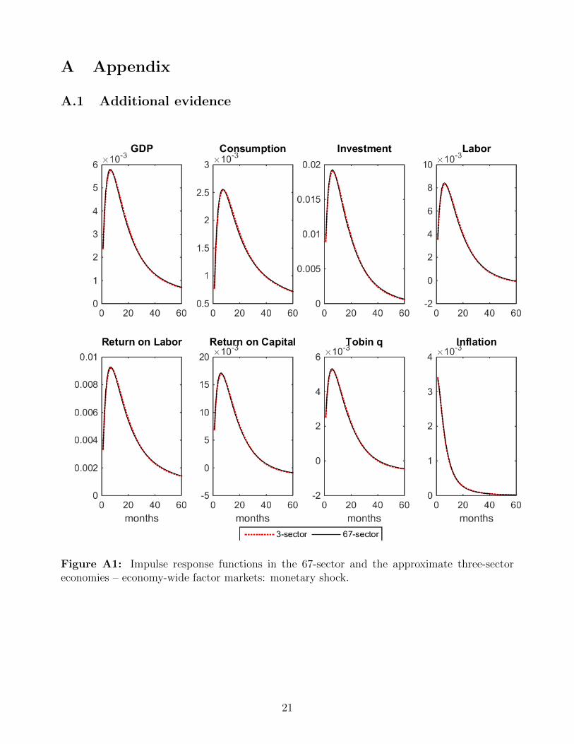
A Appendix

A.1 Additional evidence

Figure A1: Impulse response functions in the 67-sector and the approximate three-sectoreconomies – economy-wide factor markets: monetary shock.

21

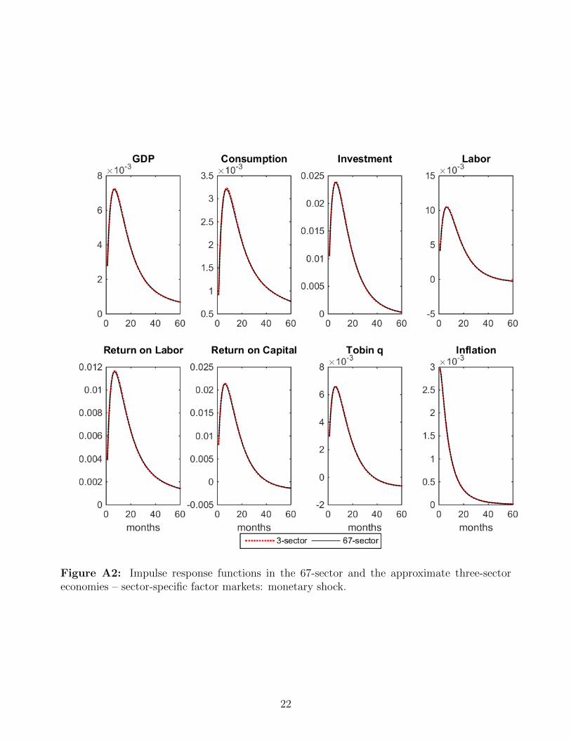
Figure A2: Impulse response functions in the 67-sector and the approximate three-sectoreconomies – sector-specific factor markets: monetary shock.

22

Figure A3: Impulse response functions in the 67-sector and the approximate three-sectoreconomies – firm-specific factor markets: monetary shock.

23

Figure A4: Impulse response functions in the 67-sector and the approximate three-sectoreconomies – economy-wide factor markets: technology shock.

24

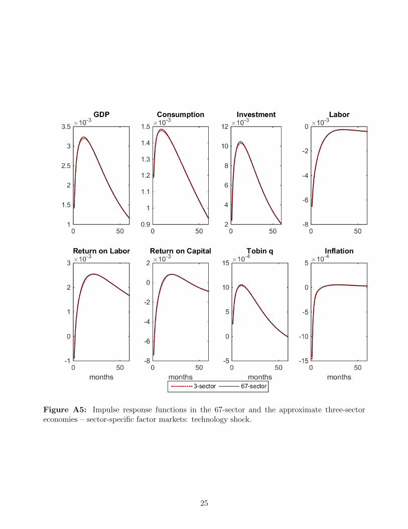
Figure A5: Impulse response functions in the 67-sector and the approximate three-sectoreconomies – sector-specific factor markets: technology shock.

25

Figure A6: Impulse response functions in the 67-sector and the approximate three-sectoreconomies – firm-specific factor markets: technology shock.

26

Figure A7: Impulse response functions in the 271-sector and the approximate three-sectoreconomies: monetary shock.

27

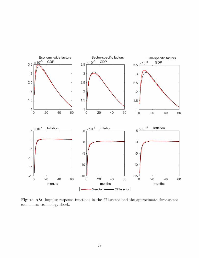
Figure A8: Impulse response functions in the 271-sector and the approximate three-sectoreconomies: technology shock.

28

Figure A9: Distribution of the cumulative approximation errors – economy-wide factor mar-kets: monetary shock.

29

Figure A10: Distribution of the cumulative approximation errors – sector-specific factormarkets: monetary shock.

30

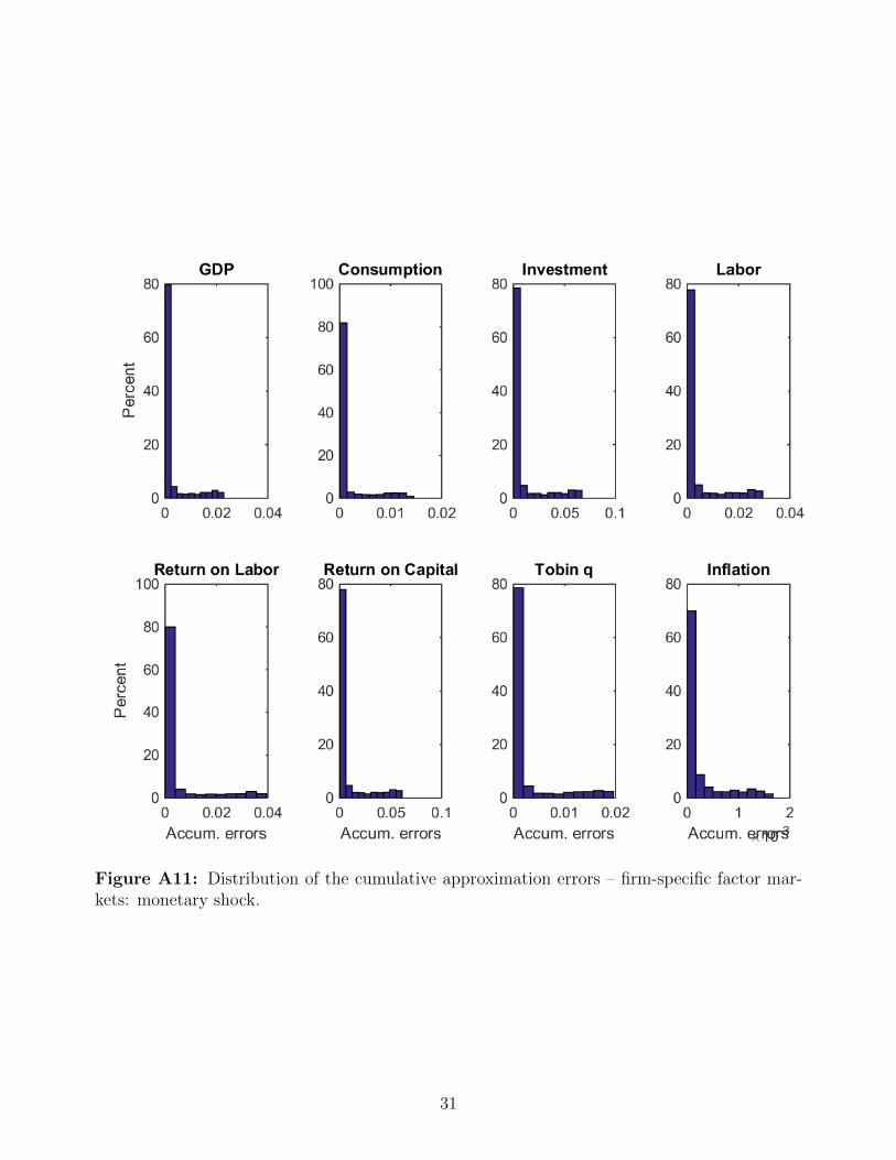
Figure A11: Distribution of the cumulative approximation errors – firm-specific factor mar-kets: monetary shock.

31

Figure A12: Distribution of the cumulative approximation errors – economy-wide factormarkets: technology shock.

32

Figure A13: Distribution of the cumulative approximation errors – sector-specific factormarkets: technology shock.

33

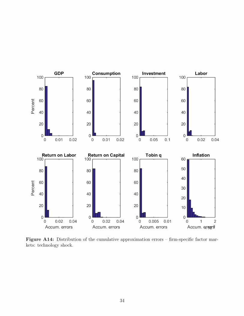
Figure A14: Distribution of the cumulative approximation errors – firm-specific factor mar-kets: technology shock.

34

Figure A15: Impulse response functions in the 67-sector and the approximate three-sectoreconomies – economy-wide factor markets: interest rate rule.

35

Figure A16: Impulse response functions in the 67-sector and the approximate three-sectoreconomies – sector-specific factor markets: interest rate rule.

36

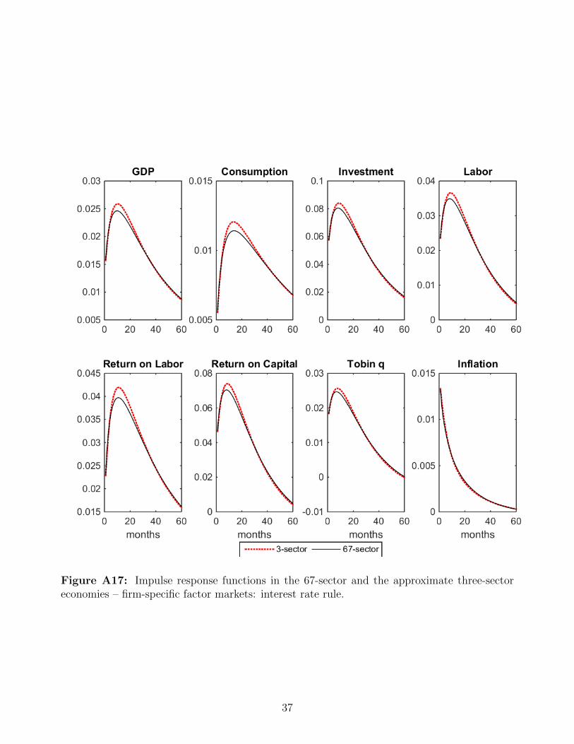
Figure A17: Impulse response functions in the 67-sector and the approximate three-sectoreconomies – firm-specific factor markets: interest rate rule.

37

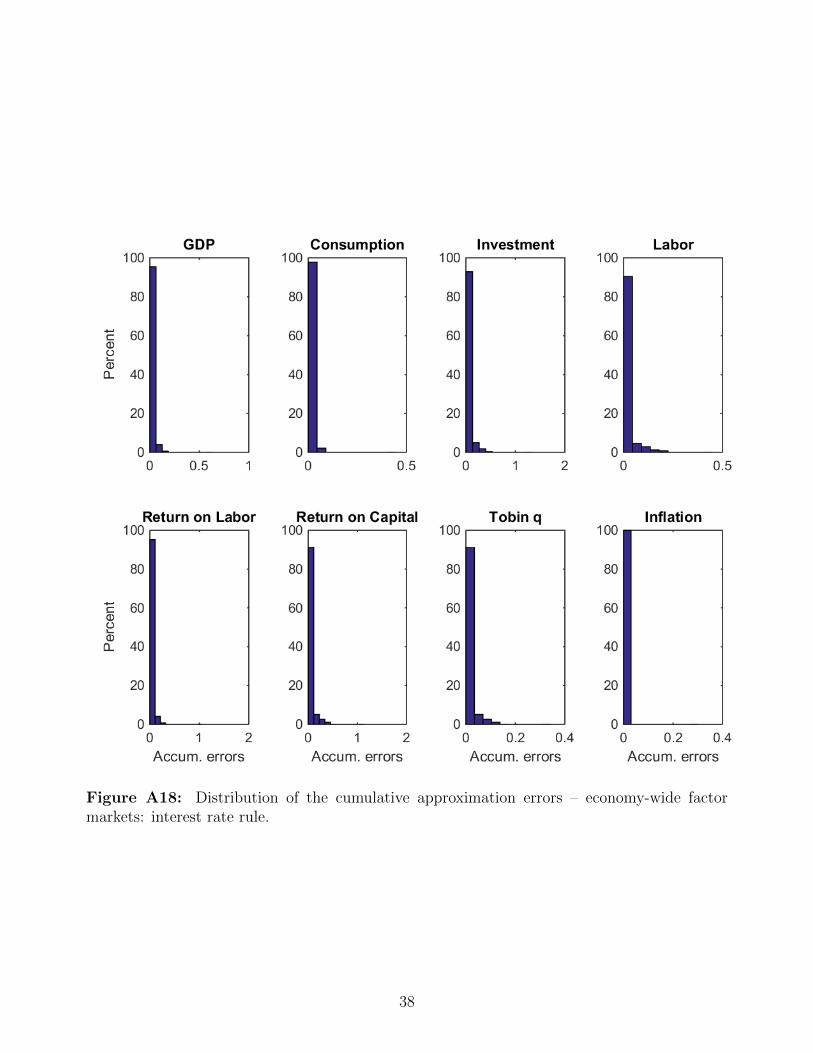
Figure A18: Distribution of the cumulative approximation errors – economy-wide factormarkets: interest rate rule.

38

Figure A19: Distribution of the cumulative approximation errors – sector-specific factormarkets: interest rate rule.

39

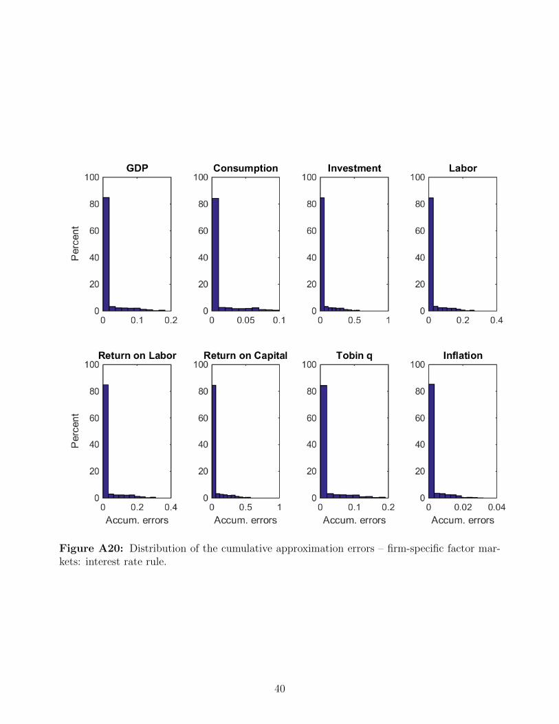
Figure A20: Distribution of the cumulative approximation errors – firm-specific factor mar-kets: interest rate rule.

40