AFGL-TR-86-0121 ENVIRONMENTAL RESEARCH PAPERS, NO. 955

AO-Am 118 Plasma Densities and Irregularities at 830 km Altitude Based on Observations During 1979

FREDERICK J. RICH MICHAEL SMIDDY

28 May 1986

a o t . )

UJ

Approved for public release; distribution unlimited.

DTI C ELECTSI k /

EP 2 4 1986 .

SPACE PHYSICS DIVISION PROJECT 2311

AIR FORCE GEOPHYSICS LABORATORY HANSCOM AFB, MA 01731

8 6 9 2 O O A 6 8

1 J->» ^.T» i--^ ij^.-i,. --,

i . '•

This technical report has been reviewed and Is approved for publication"

FOR THE COMMANDER

NELSON C. MAYNA» RITA C. SSSETO ' Branch Chief Dlr«rt-rtr \J

This report has been reviewed by the ESD Public Affairs Office (PA) and Is releasable to the National Technical Information Service (NTIS).

Qualified requestors nay obtain additional copies from the Defense Technical Information Center« All others should apply to the National Technical Information Service.

If your address has changed, or If you wish to be removed from the mailing list, or If the addressee Is no longer employed by your organization, please notify AFGL/DAA, Hanscom AFB, MA 01731. This will assist us In maintaining a current mailing list«

Do not return copies of this report unless contractual obligations or notices on a specific document requires that It be returned.

i Kn K:\-*3\ \*ri n / -yrs saasw-vA; \ß.-\ vi -vn \r\ K\\K*J\ KA <A)»JI>^>^>LTX,T,^K.V^^NK""^^S?^^-^^W

?fro5i iiJMflftW* THIS PAGt am* al REPORT DOCUMENTATION PAGE

la REPORT SECURITY CLASSIFICATION

Unclassified 1» RESTRICTIVE MARKINGS

2« SECURITY CLASSIFICATION AUTHORITY

2b OECLASSIFICATION / DOWNGRADING SCHEDULE

3 DISTRIBUTION'AVAILABILITY OF REPORT

Approved for public release; distribution unlimited.

4 PERFORMING ORGANIZATION REPORT NUMBER«)

AFGL-TR-86-0121 ERP. No. 955

S MONITORING ORGANIZATION REPORT NUMBER(S)

6« NAME OF PERFORMING ORGANIZATION

Air Force Geophysics . T ahr.ratnry

6b OFFICE SYMBOL W tpplicibl»)

PHG

7a NAME OF MONITORING ORGANIZATION

6c. ADDRESS {City, SMW, and ZV Cod*)

Hanscom AFB Massachusetts 01731

7b ADDRESS (City, Staw, and III'Code}

Ba. NAME OF FUNDING/SPONSORING ORGANIZATION

8b OFFICE SYMBOL Of applictbl*)

9 PROCUREMENT INSTRUMENT IDENTIFICATION NUMBER

8c ADDRESS (City, StaO.and ZiPCodtJ 10 SOURCE OF FUNDING NUMBERS

PROGRAM ELEMENT NO

61102F

PROJECT NO

2311

TASK NO

G5

WORK UNIT ACCESSION NO

02 11 TITLE (Includt Security CfaiiiflcationJ

Plasma Densities and Irregularities at 830 km Altitude Based on Observations During 1979 1Z PERSONAL AUTHOR(S) Frederick J. Rich and Michael Smiddy

13a TYPE OF REPORT Scientific Interim

13b TIME COVERED FROM TO "m§f$i§V'Month'o',') 15 PAGE COUNT

36 16 SUPPLEMENTARY NOTATION

17 COSATI COOES

FIELD

03 .08.

GROUP

02 ii.

SUB-GROUP

11 02

18 SUBJECT TERMS (Continuf on rtvtn» if ntatury and idtntify by block number)

Ionosphere DMSP F-region

AaOAW^vitl 19 ABSTRACT (Continue on reverse if necesiary ."vf identify by block number)

T^The in situ density of the thermal plasma was observed An-XaWwith instruments on two satellites of the Defense Meteorological Satellite Program. Each satellite was in a sun/synchronous polar orbit so that the two satellites surveyed the topside ionosphere in the mid-morning (7 to 11 hrs magnetic local time) and evening (19 to 23 hrs magnetic local time) sectors. This report presents a survey of the measured thermal ion density in order to determine the median plasma density at 830 km altitude observed as a function of latitude, longitude and season. These results are compared with plasma densities from standard models of the ionosphere, and from previous topside plasma density observations. This report also presents a survey of lowf and mid^latitude regions where plasma density irregularities are found. The plasma density irregularities in the equatorial region are presented as functions of latitude, longitude, and seasons. These regions are probably co-located with regions of Equatorial Spreadt-F radio disturbances..

20 DISTRIBUTION/AVAILABILITY OF ABSTRACT

tSuNCLASSIFIED/UNLIMITEO D SAME AS RPT DDTIC USERS

21 ABSTRACT SECURITY CLASSIFICATION Unclassified

22a NAME OF RESPONSIBLE INDIVIDUAL

OO FORM 1473,84 MAR 83 APR edition may be used until exhausted All other editions are obsolete

22b. TELEPHONE (Include Are» Code)

(617) 377-2431 22c OFFICE SYMBOL

AFGL/PHG

"""UßtiVA ION OF THIS PAGE

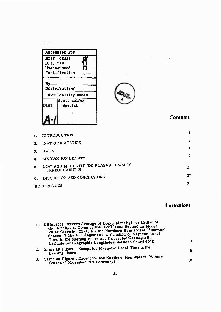
Accession For

NIIS GRAJbl DTIC TAB Unannounced Justification.

I By- Dlstrlbutlon/

Availability Codes Avail and/or

Special

1. INTRODUCTION

2. INSTRUMENTATION

3. DATA

4. MEDIAN ION DENSITY

LOW AND MID-LATITUDE PLASMA DENSITY 1KHEGULAHITIES

6. DISCUSSION AND CONCLUSIONS

REFERENCES

Contents

i

3

4

7

21

27

31

Illustrations

2.

3.

Difference Between Average of Login (density), or Median of the Density, as Given by the DMS^Data Set and the Model Value Given bv ITS-78 for the Northern Hemisphere Summer Season (7 May to 6 August) as a Function of Magnetic Local Time in the Morning Hours and Corrected Geoma8net^ Latitude for Geographic Longitudes Between 0» and 60 E

Same as Figure 1 Except for Magnetic Local Time in the Evening Hours

Same as Figure 1 Except for the Northern Hemisphere "Winter" Season (7 November to 6 February)

8

9

10

ill

liluitrationi

4. Same a« Figure 3 Except for Magnetic Local Time in the Evening Hours 11

5. Contour Plot of the Average of l.ogjg (density), or Median of the the Density. During 1979. Based on Data From the SS1E Plasma Instrument on the DMSP F2 and F4 Satellites, vs Season and the Corrected Geomagnetic Latutide of the Sub-satellite Position 12

6. Same us Figure 5 Except for Data Obtained When the r2 and F4 Satellites Were in the Magnetic Local Time Regions Later Than 12 Hours 13

7. Contour Plot of the Polynomial Fit to the AM Density Data Shown in Figure 5 16

8. Contour Plot of the Polynomial Fit to the PM Density Data Shown In Figure 6 17

!,';.. Same AM Density Contour Plot as Shown In Figure 7 Except Polar Coordinates for the Northern Hemisphere 18

9b. Same AM Density Contour Plot as Shown in Figure 7 Except Polar Coordinates for the Southern Hemisphere 19

10a. Same AM Density Contour Plot as Shown in Figure 8 Except In Polar Coordinates for the Northern Hemisphere 20

10b. Same AM Density Contour Plot as Shown in Figure 8 Except in Polar Coordinates for the Southern Hemisphere 21

11. Contour Plot of the Percentage of F2 Data Collected In the Evening Sector (magnetic local time > 12 hours) During the Fall Season of 1979 for Which the rms of Logio (density) for a 5-sec Period Exceeded 0.02 23

12. Same as Figure 10 Except for F4 Data Set During the Fall Season of 1979 24

13. Same as Figure 10 Except for F2 Data Set During All Seasons of 1979 25

14. Same as Figure 10 Except for F4 Data Set During All Seasons of 1979 26

Tables

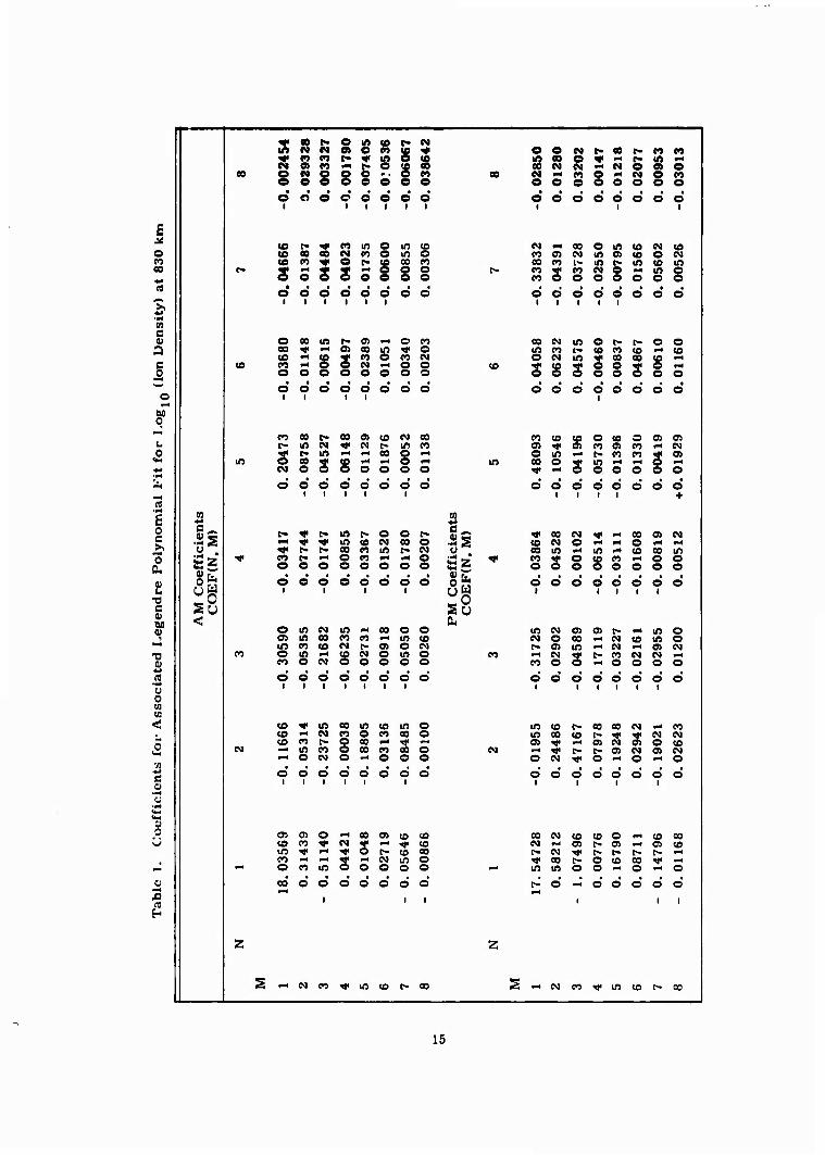
1. Coefficients for Associated Legendre Polynomial Fit for Logl0 (Ion Density) at 830 km 1U 15

2. Comparison of Median Density at 60° Magnetic Latitude Observed at 830 km Altitude by DMSP in 1979 and HILAT In 1984 29

iv

Plasma Densities and Irregularities at 830 km Altitude Based on Observations During 1979

1. INTRODUCTION

Ground-based profiles of the ionospheric density have been obtained in vast

quantities for over half a century. However, information about the ionospheric

profile above the maximum density (^F,) of the ionosphere (at 325 to 475 km

altitude) can only be obtained from satellites and incoherent scatter radar measure-

ments which are much more limited in quantity. As a result, the standard models 1 2 of the ionosphere, such as IRI 79 (Rawer et al and Rawer ) have made extensive

use of the ground-based data and have made much less use of satellite data. The

limited topside ionosphere data which has been used has been weighted more for

the f F2 altitude than for higher altitudes. We have found these models to be

inadequate when compared to topside density measurements at 830 km altitudes. Thermal plasma density measurements in the topside ionosphere have been

made with many satellites including ESRO 1A, ESRO 4, OGO 6, Alouette, ISIS I,

ISIS II, Atmospheric Explorer C and D and ISS-b. While much data from these

satellites have been published for particular seasons or latitude or longitudes, little

(Received for publication 28 May 1986)

1. Rawer, K., Bilitza, D., and Ramakrishnan, S. (1978) Goals and status of the international reference ionosphere. Rev. Geophys. Sp. Phys., UHNo. 2): 177-181, ~-..-.^~.^^~——^,:

2. Rawer, K. (1981) International reference ionosphere - IRI 79, Report UAG-82, World Data Center - A, NOAA, Boulder, Colorado.

of these data have been compiled for wide spans of latitude, longitude and seasons. 3

The best compilation to date is the ISS-b data set (Hakura, and Maruyama and 4

Matuura ). To add to the database from which a more realistic model of both the topside and bottomside ionosphere can be constructed, we have compiled all of the density data from the F2 and F4 satellites during 1979 for all latitudes (except polar regions), all longitudes and all seasons.

Since regions of irregularity in the plasma density are often associated with anomalous plasma densities, many observations of the plasma density have been excluded from the survey. However, since regions of disturbed plasma are often related to radio scintillation we also report on the probability of finding disturbed plasma, especially in the equatorial region.

The disturbed plasma near the equator is often associated with rising plumes of low density plasma in the evening sector breaking through the bottomside of the F layer and floating to the topside ionosphere. This phenomenon is generally re- ferred to as spread-F due to its signature on ionograms. The frequency of occur- rence of disturbed plasma as a function of season, latitude and longitude has been noted and is compared with previous observations. While the plasma scale lengths observed by the DMSP instrument (1 to 35 km) is greater than the scale required for radio disturbance, it is reasonable to assume that the plasma within the plumes is turbulent over a wide range of scale length up to the width of the plume.

The disturbed plasma at high latitudes is associated with the nighttime trough, the regions of precipitating particles, especially 0. 1 to 30 keV electrons, and to clouds or "blobs" of plasma density enhancement which are convected over the pole from the dayside to the nightside. These processes tend to create steep plasma density gradients with scale lengths of several km. Other process act on these steep gradients to cause plasma density of small enough scale lengths to cause degrada- tion of radio signals. Basu et al reported upon a simultaneous DMSP observation of precipitating electrons and a steep plasma density gradient and a ground observa- tion of radio scintillation.

3. Hakura, Y. (Ed.) Atlas of proton; helium ion and oxygen ion densities obtained from Ionospheric Sounding Satellite-b in situ observations October 1978 to August 1979 Radio Research Lab., Ministry of Posts and Telecommunications, Tokyo, Japan.

4. Maruyama, T., and Matuura, N. (1984) Longitudinal variability of annual changes in activity of equatorial spread F and plasma bubbles, J. Geophys. Res.. 89(No. A12):10.903-10.912.

5. Basu, A., MacKenzie, E.. Basu. S.. Carlson. H. C.. Hardy. D.A., Rich, F.J., and Livingston, R. C. (1983) Coordinated measurements of low-energy electron precipitation and scintillations/TEC in the auroral oval. Radio Sei., 18:1151-1165.

2. INSTRUMENTATION

The topside Ionospheric plasma monitor (SSIE) has been flown on several satel-

lites of the Defense Meteorological Satellite Program (DMSP) which are in polar, circular, sun-synchronous orbits. The SSIE consists of a gridded, spherical

Langmuir probe for measuring thermal electrons and a planar Faraday cup con-

figured as a retarding potential analyzer (RPA) for measuring thermal ions. The

diameter of the outer grid of the Langmuir probe is 2. 50 in. (5. 72 cm). The

aperture diameter of the planar RPA is 1. 00 in. (2. 54 cm). Both Instruments arc

mounted on a 27 in. (69 cm) boom. These instruments have been described by Smiddy et al and Rich et al' and results have been published bv Burke et al and

n Young et al. These instruments made measurements of the in situ total ion and

electron density seven times per second in the range of 10 to 10 cm" . Any density

greater than the maximum of the instrument is reported in the telemetry as the

highest possible value [log.Jdensity) = 6. 1]. They also made measurements of the

ion and electron temperature once each 64 sec and in the range of 800° to 10, 000oK.

These instruments use a single range, logarithmic amplifier and a nine-bit analog-

to-digital conversion. The least significant bit of the telemetry represents a change

of density of log _ (density) of 0. 01. Relative changes (changes from one moment

to the next due to local variations) in density of 2 percent are clearly described.

The absolute density is a function of the calibration and the spacecraft-plasma

interaction. It is estimated to be accurate to better than 25 percent in density or

better than ± 0. 10 in log 10 (density).

In flight, only the total ion density (which is equivalent to the ambient electron

density) can be measured whenever the satellite is in sunlight which is approximately

80 percent of the time. This is due to a spacecraft potential caused by unshielded

contacts on the solar cell array, which tends to attract electrons and repel ions.

6. Smiddy, M., Sagalvn, R. C., Sullivan, \V. P., VVildman, P. J.L., Anderson, P., and Rich. I". (1978) The Topside Ionosphere Plasma Monitor (SSIE) for the Block 5D Flight 2 DM5P Satelllie, Report AFGL-TR-7fl-OD71, AD A058503, Hanscom AFB, Massachusetts.

7. Rich, F., Smiddy, M., Sagalvn, R.C.. Burke, W..I., Anderson, P., Bredesen, S., and Sullivan, W . P. (1980) In-flight Characteristics of the Topside Ionospheric Monitor (SSIE) on the DMSP Satellites Flight 2 and TTtght 4, Report AFGL-TR-80-0152, AD A088879, Hanscom AFB, Massa- chusetts.

8. Burke, W. J., Donatelli, U.K., and Sagalvn, R. C. (1980) The longitudinal distribution of equatorial spread F plasma bubbles in the topside ionosphere, .1. Geophys. Ucs. , 85:1335-1340.

9. Young. E. R., Burke. W Rich« F..J., and Sagalyn, R. C. (1984) The distribu- tion of topside spread-F from in situ measurements by Defense Meteorological Satellite Program F2 and F4, J. Geophys. Rea., M(No. A7):5565-5574.

Thus the vehicle is driven to negative potentials of -20 V to -32 V. The measured

ion current is unaffected by the positive potential because the spacecraft velocity is

much greater than the ion thermal motion, and because ions which are deflected toward the sensor are collected by the external case of the sensor and a ground

plnne »round the ion sensor. Flight 2 U*2) of the most recent generation of DMSP spacecraft was launched in

.June 1'JTT into a 820 km ultitude, OU. 1° inclination, circuiur orbit and carried the

first of the SSIK instruments. Both the F2 satellite und the SSIli instrument operated

continuously until January I OHO, The F2 satellite was not quite in a sun-synchronous

orbit but in an orbit that shifted approximately one-half hour in local time per year.

In 1979, F2 was approximately located with the ascending node at 0930 hours and

descending node at 2130 hours geographic local time. Might 4 (F4) was launched

in .lune 1970 into a 830 km altitude. 98.7° inclination, circular orbit with the

second of the SSIE instruments. Both the F4 satellite and the SSIE instrument

operated continuously until February 1980. From February 1980 to August 1980,

intermittent data were obtained. The F4 satellite was located with ascending node

at 2310 hours and descending node at 1010 hours geographic local time. Due to the

offset between the magnetic and geographic axes, the two satellites sampled a

region of magnetic local time approximately one hour to either side of the geographic

local times given above while they were at low latitudes and a slightly wider range

of magnetic local times at higher latitudes.

3. DATA

The total ion or electron density data were compiled for the period 1 January

1979 to 31 December 1979. This represents 12 months of F2 data and 6 months of K4 flutu. Data wort- available for 95 percent to 98 percent of each day of data collec-

tion. Data were collected in a format usable for this study on 90 percent of the

pos.sibU clays'. The data were first compiled as 5-SPC averages of the seven samples -3 per second values of log.Q (density (cm ]). Because of uncertainty in knowing the

density when the current to the sensor reached saturation, the few data points equal

to this maximum value have been discarded from the database. Because the ion

density measurements are not affected by the spacecraft potential, almost all of the

data come from the ion sensor. In addition, the root-mean-square (rms) of

log.»(density) for each 5-scc period was also calculated und saved. These two

values, plus a time tag and ephemeris information, were saved for further proces-

sing.

Since the data are given and used In terms of log10(density) instead of density,

the average values represent the median of the density (a geometric mean). A

median value Is generally best in comparing future data sets to past results when

the underlying process is normally quite variable. For regions where the distribu- tion of values covers a small range, the geometric mean is almost equivalent to the arithmetic mean. In cases where there Is a wide variation in density (up to two

orders of magnitude in the polar regions), the geometric mean is less than the

arithmetic mean.

Because the ionosphere is strongly controlled by the geomagnetic field, a

coordinate system based on the magnetic field should be used to represent the data.

We have chosen to use the corrected geomagnetic coordinate system of Gustafsson '

for epoch 1965. We have done this by taking the geographic latitude and longitude of

the satellite for zero altitude and using Gustaffson's table. This avoids the discon-

tinuity in the invariant latitude system as the satellite crosses the equator and also

avoid problems with the dip-iatitude system near the poles.

The next step consisted of gathering the data into a series of statistical bins.

Into each bin is placed the average value of log..(density), or median density, _if

the rms of the 5-sec average was less than a given value. The data were first

sorted into bins representing: (a) 3s of magnetic latitude, (b) 0. 25 hour of mag-

netic time, (c) 60° of geographic longitude, (d) 3 months of the year, and (e) each

satellite. From this survey, we concluded that the variation in magnetic local time

was not significant enough to justify the small divions, but the seasonal variation

was not adequately described. Thus we re-generated our survey into bins

representing: (a) 60° of geographic longitude, (b) 3° of corrected geomagnetic

latitude, (c) 9 or 10 days, (d) either AM or PM magnetic local time and (e) each

satellite for a total of 6 by 60 by 40 bins by 2 bins by 2 bins. At first, we used a criterion of rms of the 5-sec average of log.-(density) S 0. 02,

for all locations when selecting data to be included in a bin. This procedure elimi-

nates occasional bad data points and data in regions with sharp density gradients

and/or disturbed plasma. In particular, we wished to eliminate regions of equa-

torial bubbles, which are associated with spread-F. where the density can decrease 2

by a few percent to a factor of 10 over a short distance and significant, small-scale

density variations in the high-latitude regions. By keeping track of the percentage

10. Gustafsson, G. (1970) A revised corrected geomagnetic coordinate system, Arkiv fur Geophysik, 5:595-616.

11. Gustafsson, G. (1984) Corrected geomagnetic coordinates for epoch 1980, Magnetospheric Currents, T. A. Potemra, Ed., Am. Geophys. U., Washington, D. C.

of data discarded by this criteria, this survey was used to look for the longitude, latitude and seasonal variations of the occurrence of the low latitude and mid- latitude density irregularities.

While the above criterion for selecting 5-sec averages was good for surveying the occurrence of low and mid-latitude density irregularities, it was not good for a global survey of the median plasma density. Much of the high latitude 5-sec aver- ages were eliminated from the survey when the criterion of 0. 02 for deviations was used. Specifically, the probability of occurrence of irregular plasma during a 5-sec sampling period using this criterion at high latitudes was always in the range of

12 40 percent to 100 percent. By comparison, Clark and Raitt found a probability of 20 percent to 30 percent for 0. 2-sec sampling periods using a criterion of the rms of the 'ensity exceeding 10 percent (which is approximately equal to a rms of log 10 (density) of 0. 04). By using a criterion of the rms of the density exceeding 5 percent Clark and Raitt found probabilities of occurrence of 20 percent to 60 percent in the high latitude regions.

For a survey of the median plasma density, we did a separate survey using the criteria of:

rms of 5-sec sample of log.Jdensity) S 0. 02 for -30» to +30° S 0. 10 for -60s to -30°

and +30" to+60'' (1) g 0.50 for -90» to -60°

and +60° to +90° .

The low latitude criterion is the same sample as that used in the irregularity survey and the high latitude criterion is chosen to be so large that almost all data not effected by telemetry errors are selected. The mid-latitude criterion was chosen to allow a transitirn between the high and low latitude regimes.

12. Clark. D.H., and Raitt, W.J. (1975) Characteristics of the high-latitude ionospheric irregularity boundary, as monitored by the total ion current probe on ESRO-4, Planet. Space Sei., J23:1643-1647.

13. Clark, D.H.. and Raitt, W.J. (1976) The global morphology of irregularities in the topside ionospheric as measured by the total ion current probe on ESRO-4. Planet. Space Sei.. ^24:873-881.

4. MEDIAN ION DENSITY

Ion density in the Ionosphere as a function of latitude, longitude, time of day, 14 season, and solar activity Is given by models such as ITS-78 (Barghausen ) and

2 IRI-79 (Rawer ). The ITS-78 model was based almost exclusively on measure-

ments made from the ground up to the maximum density of the F-region at 350 km

to 600 km altitude. The IRI-79 model has used topside density data from the

Alouette topside sounder. However, these data were weighted more heavily for

measurements near fFS than for high altitudes. As a result. It Is not obvious the

model densities at 830 km altitude should match the observed densities.

Our first task was to compare the measured median density with the density

from previous models to determine if the previous models were accurate enough for

future work in the topside ionosphere. In Figures 1 through 4 we have plotted the

difference of log 10(density) between the DMSP median density and the ITS-78 model

density. Only one longitude sector is shown as an example. For some areas the

difference is less than 0. 3 (a factor of two in density) which is acceptable for much

work, but the difference is 1. 0 (a factor of ten in density) or more in other areas.

In particular, the ITS-78 model is very poor in the mid-latitude region of the winter

hemisphere. We have not made as thorough of a comparison of the observed densi-

ties with the IRI-79 model, but we h-ive similar differences. As a result, we have

proceeded to create a complete survey of the region of space observed by the DMSP

satellites for 1979.

Figures 1 through 4 and similar representations of the data set showed that the

small bin size for magnetic local time were not a necessary element of the analysis.

For the morning or evening sector, the variations in log 10 (density) are generally

less than 0. 3 (a factor of two in density). In addition, there are large sections of

the magnetic latitude vs magnetic local time grid in Figures 1 through 4 that have

no data (the unshaded area). Thus, our further analysis is for only two" local time

zones (local times < 12 hours, denoted as AM, and local times > 12 hou.rs, denoted

as PM).

14. Bargha isen, A. F., Finney, J.W., Proctor, L. L., and Schultz, L.D. (1969) Predicting long-term operational parameters of high-frequency sky-wave telecommunication systems. ESSA Technical Rep. ERL 110-ITS 78, U.S. Govt. Printing Office, Washington, D. C.

LOGCNDMSP) - U)G(NITS78)

SüMNER 1979 GEOGRAPHIC LONGITUDE »O'TOeO'E

« 3 K g

-30°-

MAG UDCAL TIME(HRS)

Figure 1. Difference Between Average of Log ^(density), or Median of the the Density, as Given by the DMSP Data Set. id the Model Value Given by ITS-78 for the Northern Hemisphere "Summer" Season (7 May to 6 August) as a Function of Magnetic Local Time In the Morning Hours and Corrected Geomagnetic Latitude for Geographic Longitudes Between 0° and 60°E

The values of log 10(denslty) were collected, as described In Section 3, for the global survey of the median plasma density. The three levels of the rms of logl0(density) which were used were chosen to eliminate the density decrease& related to equatorial bubbles, the sharp gradients associated with the walls of

extremely deep mid-latitude troughs, the sharp density gradients associated with local, intense auroral precipitation zones and with occasional bad points due to errors in the telemetry.

UWNDMSP) " LJOGtNnsTe)

SUMMER 1979 GEOGRAPHIC LONGITUDE = 0° TO 60° E

20 21 22

MAG LDCAL TIME(HRS)

Figure 2. Same as Figure 1 Except for Magnetic Local Time in the Evening Hours

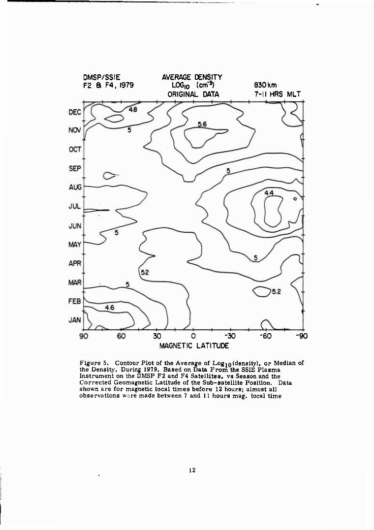
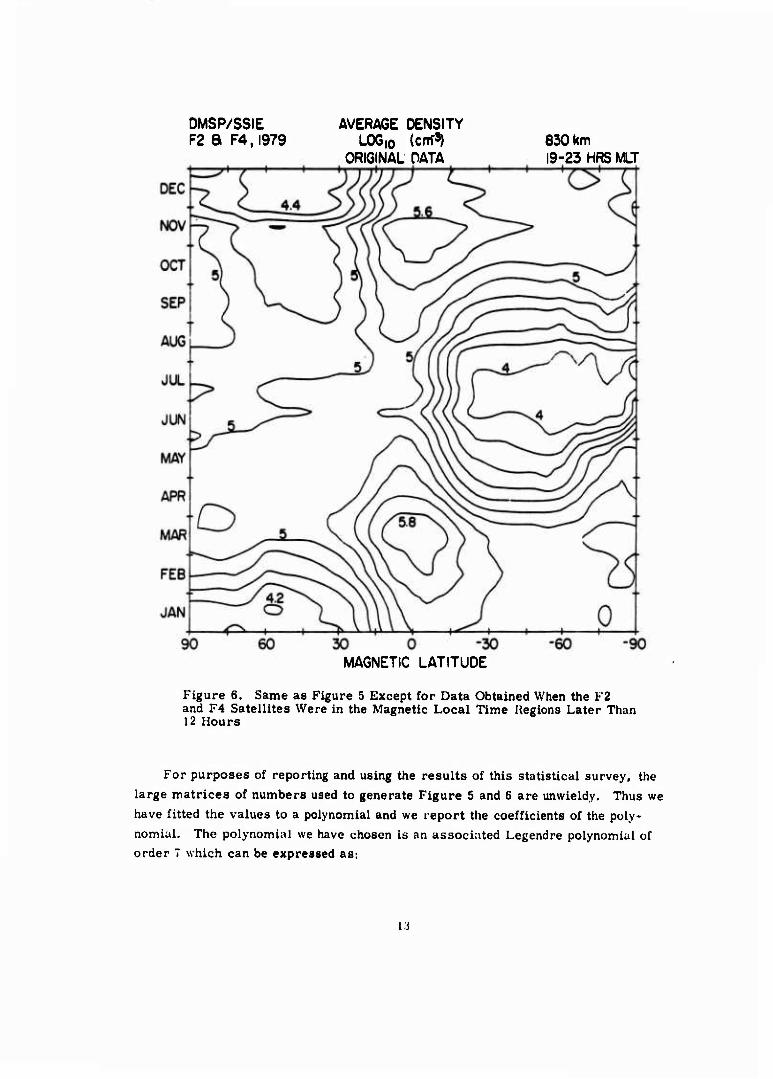
The values of logl0 (density) were analyzed as a function of longitude and found to have no systematic variation with longitude within a factor ± 0. 3 in log .-(density) or a factor of two in density. Thus, we have grouped our data for all longitudes together into a single bin for the creation of our survey of the median density. The result is a set of two matrices of average log.Q(density), or median density, vs magnetic latitude and season. Figures 5 and 6 represent the matrices for the AM and PM time zones, respectively. As expected, the density near the equator tends to be greater than the density at mid- and high latitudes. The maximum values represented in Figure 6 near the equator in March may be slightly less than the true value because the ionospheric density occasionally exceeded the limits of the instrument and these points were removed from the data before the median was calculated.

UXSWDMSP) - UWNITSTO)

60« WINTER 1979 GEOGRAPHIC ÜONGITUDE « 0* TO 60» E

D t

§ J Ü

I I -30-H 2

-60°- "T"

7

MAG LOCAL TIME(HRS)

Figure 3. Same as Figure 1 Except for the Northern Hemisphere "Winter" Season (7 November to 6 February)

At mid- and high latitudes, the density is lower In the winter season (November to February for the Northern Hemisphere and May to August in the Southern Hemis- phere) than in the summer season. The winter density in the Southern Hemisphere (May to August), low density region in Figures 5 and 6 is lower than the winter density in the Northern Hemisphere (November to February). This is the same

15 result as reported by Sojka et al except that the region of low density on average

15. Sojka, J.J.. Raitt, W,J., Schunk, R. W., Parish, J.L., and Rich, F.J. (1985) Diurnal variations of the dayslde, ionospheric, mid-latitude trough in the Southern Hemisphere at 800 km; model and measurement comparison. Planet. Space Sei. . 22:(No- 12):1375-1382.

10

LOG(NDMSP) - U)G(N|TS78) WINTER 1979 GEOGRAPHIC LONGITUDE «0° TO 60° E

60«

UJ 30°- o Z)

-1 o0-

< -30°-

-60« 19 20

-*r 21 22

MAG IDCAL TIME(HRS)

23

Figure 4. Same as Figure 3 Except for Magnetic Local Time in the Evening Hours

extends to lower latitude than previously noted. This implies a connection between the high and mid-latitude ionosphere regions since the lower density reported by

15 Sojka et al is due to a combination of the high latitude convection pattern and the offset of the geomagnetic pole from the geographic pole.

U

DMSP/SSIE F2 a F4, 1979

AVERAGE DENSITY LOGio (cm*3)

ORIGINAL DATA 830 km 7-11 HRS MLT

30 0 -30 MAGNETIC LATITUDE

90

Figure 5. Contour Plot of the Average of LogJQ (density), or Median of the Density. During 1979. Based on Data From the SSIE Plasma Instrument on the DMSP F2 and F4 Satellites, vs Season and the Corrected Geomagnetic Latitude of the Sub-satellite Position. Data shown are for magnetic local times before 12 hours; almost all observations wire made between 7 and 11 hours mag. local time

12

DMSP/SSIE F2 & F4,I979

AVERAGE DENSITY LO610 (crrf3)

ORIGINAL DATA 830 km 19-23 HRS MLT

30 0 -30 MAGNETIC LATITUDE

Figure 6. Same as Figure 5 Except for Data Obtained When the F2 and F4 Satellites Were in the Magnetic Local Time Regions Later Than 12 Hours

For purposes of reporting and using the results of this statistical survey, the large matrices of numbers used to generate Figure 5 and 6 are unwieldy. Thus we have fitted the values to a polynomial and we report the coefficients of the poly- nomial. The polynomial we have chosen is an associated Legendre polynomial of order 7 which can be expressed as:

li

7 n log,-(ion density) - Z 2 c"1 b" v"1 (2)

10 n-0 m-.n n n n

where

x « corrected geomagnetic latitude/90°,

y = Day Number * 2jr/365,

Y"1 = cos (m y> P"1 for m = (0, n).

= sin (m y) P™ for m = (-n. -1),

cJJ1 = fitting coefficient,

b"1 = normalization factor, and n

Pm = associated Legendre polynomial.

The functions b"1 and P™ are defined as: n n

b0 = J2n)l l(2n+1)/4ff]l/2 O) n 2n (nl )*

.m (2n) :n: I(2n+ 1) (n-m) ' 1/2

2n(n:)Z(n-m) ' 2" ^+m> '^

P0 = 1

P" = (1-x2) P"-1, n n - i

P" = xP" - R"1 Pnm

2 n n- 1 n n-2

where

2 2 Rm _ (n- 1) - m „n - 1 _ n "n " (2n-l) (2n-3) ' "n ~ u "

The fitting coefficients are given from the parameters COEF(N, M) in Table 1 by the relationship:

COERN'.M) = C^.^1 forNSM (4)

COEF(N, M) = CM \ * for N < M .

14

o n oo

to c 0)

§

0

£ 0 c Si o

c

0)

■u

u 0 10 (0 <

^2 e o

5

<

CM 0> O N o e

o m to t> N o» o «o «e « t« ^ in e <p

o (0 S -. o M o o o s

d o e • c

1 o

1

• o

1

• o

1 d

to

to

s 00 M

o

s s

CM o s

in «

o

o o

in m 00

§

to o n o o

• • • • • • • •

ooeMt>eet>eom Sop o <*••-< t» m «

<S C4 <-< N o e> o

oooooooo

dddddddd i i i

MM« o m to eg <o eoo>eMino>(OOC4 ooni»int«iAioin «♦eoNO-tinÖ MOOOOOOO

o o o i i

o I

o o I I

o o

oooinr-o>>*om ooT("MO>cein^<o co^eoNMOO oooooooo o o o o o o o

CO

s 00 in

00 o

IA

s 00

s 0> CM

o

to

00

o

M in

§ o

« CO

•-* o

o o 1 o o

i o

1 o o

i o

CO o 5 •-4

O

in m 00

§ CD M (0 o

o m *-* o

o eo

o

o CM o o

o i

o o 1 o o

1 o o o

o OS m o CO

m m M

S co to

m CO M

M

o

00 11

O) o o

o m o m o

o CO

o o

o i o

1 o

1 O o

1 d o

i o

1 i Ü

o Si u ̂ s Ü a.

N

(O^inoomcoino (O^MCOOCOCOO «eot-Oooi-i^«-" "incoooocoooo — ONO-«OOO

M

o o o o o I I I I

o o I

d i d d

i d i d

i d d d

0405

8 06

232 in

m s

o CO to

00

s o

s o

o CO •-4

o o o o o

1 o O o o

CO « o oo

CO

s o i

o eo

CO

o

o eo CO

o

0>

o

OS CM OS f-4

o o o

i o

1 o o

i o o o

+

CO oo CO o

00 N in

s CM o o o

in n o

00 o CO t-H

o

03

00 o o

CM

s o

o 1 o o o

■ o i o

1 o

1 d

in M

CO

CO

CM o

05 00 in

3

0)

s «o

CM o

in m 0) CM o

§ CM

O

o 1 o o

1 o

1 O

I o

1 o o

m in OJ

o

CO 00 CO

oo

03

o

00

~4

CM

3 CM o

CM o 05

eo N CO CM o

o o o I I

o o o o o

O505O «10005GOCO coeo4>CM*ii-i^ico mTfr-TfOt^toeo co-"»*«i-«cMinO oeomooooo

oo d d d d d d d

I I I

OOCMCOCOO^COOO e>)"-05t->03"H03CO t-CM^<t»t»t-t*<-" «^OOt-OCOOOTf-i mmoo — o — o r- o -H o o o o o

i i

s - N co ^< m co f- oo 2 - CM co ^ in co

15

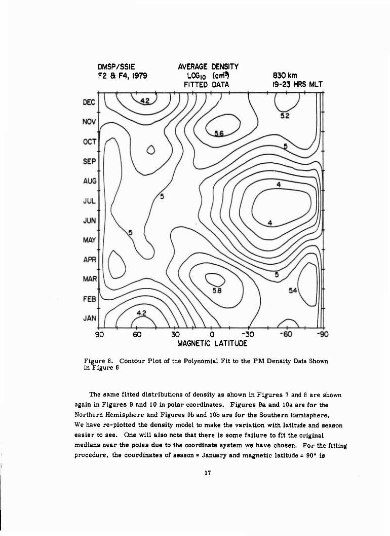
Figures 7 and 8 represent the results of the fitting polynomial In the same format as Figures 5 and 6 for the original binned medians. Clearly all of the major components of the distribution shown In Figures 5 and 6 are reproduced In Figures 7 and 8.

DMSP/SSIE F2 8 F4, 1979

90

AVERAGE DENSITY LOGio (cm3) FITTED DATA

830 km 7-11 HRS MLT

60 30 0 -30 MAGNETIC LATITUDE

Figure 7. Contour Plot of the Polynomial Fit to the AM Density Data Shown in Figure 5

16

DMSP/SSIE F2 a F4, 1979

AVERAGE DENSITY LOGio (cnft

FITTED DATA 830 Km 19-23 HRS MLT

90 60 30 0 -30 MAGNETIC LATITUDE

Figure 8. Contour Plot of the Polynomial Fit to the PM Density Data Shown in Figure 6

The same fitted distributions of density as shown in Figures 7 and 8 are shown again in Figures 9 and 10 In polar coordinates. Figures 9a and 10a are for the Northern Hemisphere and Figures 9b and 10b are for the Southern Hemisphere. We have re-plotted the density model to make the variation with latitude and season easier to see. One will also note that there Is some failure to fit the original medians near the poles due to the coordinate system we have chosen. For the fitting procedure, the coordinates of season = January and magnetic latitude = 90a Is

17

identical to the coordinate of July and 00*, which is logically incorrect. The result is that the fitted values are invalid between 80* (or -80°) and the pole. Between 60° and 80s (or -60s and -80°), the fitted value is not as accurate as the original data and should be used only with great care.

DMSP/SSIE F2 a F4, 1969

OCT

AVERAGE DENSITY 1)06,0 (cnT») FITTED DATA

NORTHERN HEMISPHERE 830 km

7-11 HRS MLT

JUL JUN

APR

MAR

Figure 9a. Same AM Density Contour Plot as Shown in Figure 7 Except Polar Coordinates for the Northern Hemisphere

18

DMSP/SSIE F2 8 F4, 1979

AVERAGE DENSITY LOG» (crrf») FITTED DATA

SOUTHERN HEMISPHERE 830 km

7-11 HRS MLT

Figure 9b. Same AM Density Contour Plot as Shown in Figure 7 Except Polar Coordinates for the Southern Hemisphere

Only on a few occasions has the DMSP spacecraft potential allowed mass data to be obtained with the RPA. For F2, i'.is has occurred only when the satellite is in darkness. For F4, we were able to make some special studies where the potential of the instrument could be biased away from the satellite potential and toward the plasma potential. On these occasions, the density at all latitudes in the AM sector is composed for > 90 percent 0+ ions. In the PM sector during the winter season, we find that light ions (H+ and He+) make up 10 percent to 60 per- cent of the total density in the mid-latitude regions of the low density. While we

19

DMSP/SSIE F2 a F4, 1979

AVERAGE DENSITY LOG«, Icttf») FITTED DATA

JUL JUN

NORTHERN HEMISI'HERE 830 km

19-23 MLT

OCT

DEC JAN

Figure 10a. Same AM Density Contour Plot as Shown in Figure 8 Except in Polar Coordinates for the Northern Hemisphere

cannot conclusively distinguish the H+ from the He+ ions, our data indicate that the majority of the light ions observed In the winter are He+. This mass distribu- tion Is consistent with the "helium bulge" which has been previously reported. A systematic survey of the available mass distribution data from the DMSP plasma instrument has not been made. Measurements from other satellites and ionos- pheric models generally indicate that the ionosphere at 830 km altitude is dominated by Of Ions.

20

OMSP/SSIE F2 a F4, 1979

AVERAGE DENSITY LO610 (cm») FITTED DATA

SOUTHERN HEMISPHERE 830 km

19-23 MRS MLT

JUL JUN

OCT

DEC

Figure 10b. Same AM Density Contour Plot as Shown in Figure 8 Except in Polar Coordinates for the Southern Hemisphere

5. LOW AND MID-LATITUDE PLASMA DENSITY IRREGULARITIES

An irregular plasma is any plasma which has small scale density gradients.

The definition of small scale depends on the system being studied. At lov^and mid

latitudes, the ionospheric plasma generally has scale lengths of the density gra-

dients of the order of 100 to 1,000 km except in regions of turbulent plasma. By

selecting plasma measurements by the criteria of the rms of a 5-sec (37 km)

average of log 10 (density), or median of the density, being greater than 0. 02, we

21

can find regions of plasma gradients smaller than 100 km. Then by arranging the selected "irregular" plasma measurements according to season« geographic longi-

tude and magnetic latitude, we can find the probability of encountering the

"irregular" plasma at a given time and location. The "irregular" plasma can in

turn be related to degradation of radio propagation, especially in the equatorial i fi 17'

region (Basu et al and DasGupta et al ).

As might be expected, the probability of encountering "irregular" plasma

density regions at low and mid-latitudes in the morning sector is low (less than

10 percent of the observation) for all longitudes and all seasons. In the evening

sector, there is a significant probability at certain locations and seasons. Figures

11 and 12 show the probability of encountering plasma that is "irregular" according

to the rms of the 5-sec average of log ..(density) > 0. 02 criteria for F2 and F4

respectively during the Fall season of 1979 (7 August to 6 November). There are

two zones of "irregular" plasma clearly evident: (a) near ±60° magnetic latitude,

and (b) within 20° of the magnetic equator. The first region is mostly an extension

to lower latitudes of the high latitude plasma region were the probability of rms

exceeding the value of 0. 02 is always very high. In addition, plasma irregularities

are common on the equatorward edge (magnetic latitude =45° to 60°) of the evening, 18 mid-latitude trough (Basu ).

The second region is probably related to plasma bubbles which cause the 19 "spread-F" signatures In ionograms (Hanson et al ). These bubbles are regions

of low density plasma that are created near the steep bottomside gradient of the

F-region shortly after sunset due to the Rayleigh-Taylor instability. The bubbles

then drift upward to the altitude of the DMSP satellite and beyond. Typical

dimensions for these bubbles are approximately 100 to 200 km in the east-west and

vertical directions and 500 km to a few thousand km in the north-south direction

along magnetic field lines. In fact, as the bubbles drift upward, they elongate in

the north-south dimension.

16. Basu, S., Khan, B. K., and Basu, S. (1976) Model of equatorial scintillation from in situ measurements. Radio Sei., 11:821;832.

17. DasGupta, A., Aarons, J., Klobuchar, .J.A. , Basu, S., and Bushby, A. (1982) Ionospheric electron content depletions associated with amplitude scintilla- tions in the equatorial region, Geophys. Res., Letters, 9(No. 2); 147-150.

18. Basu, S. (1978) Ogo 6 observations of small-scale irregularity structures associated with subtrough density gradients, J. Geophys. Res., 83(No. Al):182-190.

19. Hanson, W. B., McClure, J.P., and Sterling, D. L. (1973) On the cause of equatorial spread F, J. Geophys. Res., 28:2353-2356.

22

DMSP/F2SSIEI979 FALL PERCENTAGE OF OCCURENCE OF IRREGULARITY IN EVENING SECTOR

90* 180» 270*

GEOGRAPHIC LONGITUDE 360»

Figure 11. Contour Plot of the Percentage of F2 Data Collected in the Evening Sector (magnetic local time > 12 hours) During the Fall Season of 1979 for Which the rms of Logjo (density) for a 5-sec Period Exceeded 0. 02. This criteria indicates the locations of disturbed plasma

In many cases, the identification of plasma bubbles can be confirmed because the plasma density inside one of these bubbles may be less than the density in the

3 surrounding region by as little as 20 percent or as large as a factor of 10 . This yields a significant plasma density gradient on the edges of the bubble. In addition. the plasma in and near the bubble tends to be very turbulent: this turbulence also yields significant plasma density gradients. An investigation of the longitudinal and local time distribution of obvious plasma bubbles has been presented by Young

9 et al. In many other cases, the identification of plasma bubbles cannot be con- firmed by a drop in the 5-sec average of log..(density). However, since these disturbances have the same latitudinal and local time distributions, it is reasonable to assume that these disturbed plasma regions are either the tops or sides of plasma bubbles. In proof of this assumption, we can refer to one case when the F2 and F4 satellites were near Ascension Island nearly simultaneously with the passage of the Atmospheric Explorer E satellite and when simultaneous ground observations were being made. The F2. AE-E and ground observations clearly

23

DMSP/F4 SSIE 1979 FALL PERCENTAGE OFOCCURENCE OF IRREGULARITY IN EVENING SECTOR

60» mmmtmtm

90* 180° 270*

GEOGRAPHIC LONGITUDE

360«

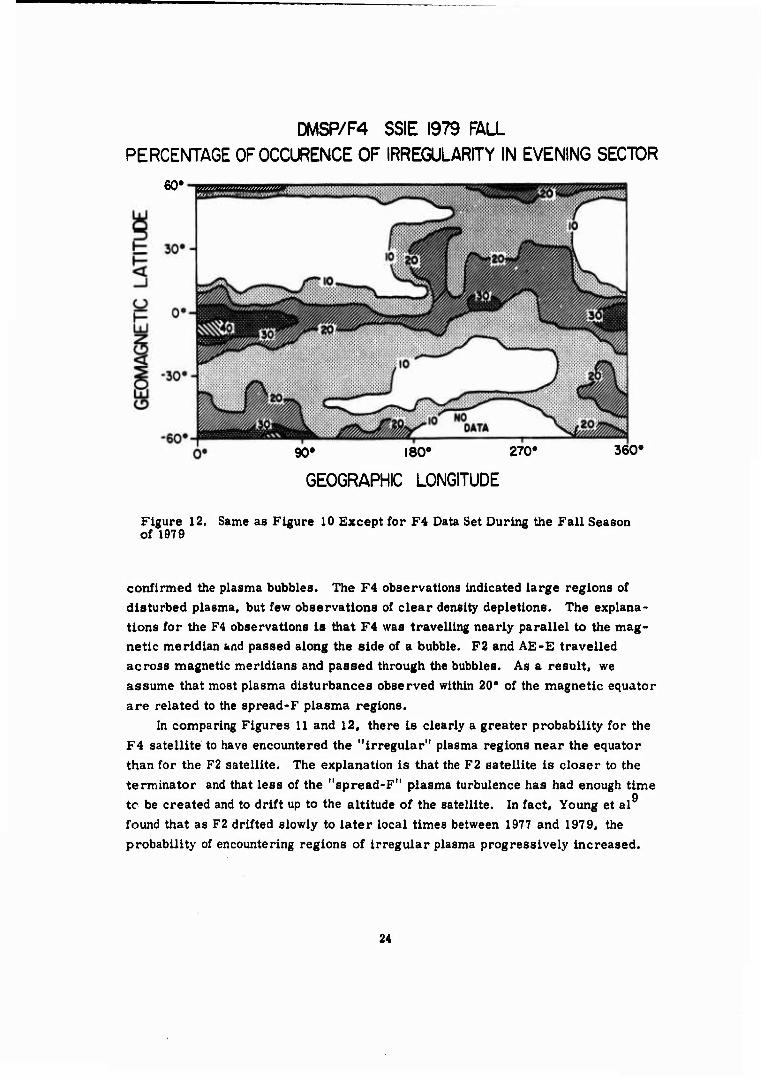
Figure 12. Same as Figure 10 Except for F4 Data Set During the Fall Season of 1979

confirmed the plasma bubbles. The F4 observations indicated large regions of disturbed plasma, but few observations of clear density depletions. The explana- tions for the F4 observations is that F4 was travelling nearly parallel to the mag- netic meridian and passed along the side of a bubble. F2 and AE-E travelled across magnetic meridians and passed through the bubbles. As a result, we assume that most plasma disturbances observed within 20° of the magnetic equator are related to the spread-F plasma regions.

In comparing Figures 11 and 12, there is clearly a greater probability for the F4 satellite to have encountered the "irregular" plasma regions near the equator than for the F2 satellite. The explanation is that the F2 satellite is closer to the terminator and that less of the "spread-F" plasma turbulence has had enough time

a tc be created and to drift up to the altitude of the satellite. In fact. Young et al found that as F2 drifted slowly to later local times between 1977 and 1979, the probability of encountering regions of irregular plasma progressively Increased.

24

Previous investigations have indicated u seasonal control of the occurrence of 20 low latitude plasma irregularities. For example. Aaron et al used radio scin-

tillation data and found a minimum in the probability of occurrence during the summer (May to July) and winter (November to January) seasons. This survey of plasma irregularities has also found that there is a seasonal dependence to the probability of encountering low latitude regions of disturbed plasma. The prob- ability is greatest in the Spring and Fall (Figures 11 and 12), but there is a sig- nificant probability of encountering regions of irregular plasma in all seasons. Figures 13 and 14 represent a summary of the probabilities for the entire data set. For F4 the probability is weighted toward the Fall season because of a lack of data in the first six months of the year.

DMSP/ F2 SSIE 1979 SUMMARY PERCENTAGE OF OCCURENCE OF IRREGULARITY IN EVENING SECTOR

LÜ Q 3

60*

30«

i -30»-

-60'

:-::'-:V:

:::AV".

::V-:V:-^I*'"*'

O* 90» IBO»

GEOGRAPHIC LONGITUDE 360

Figure 13. Same as Figure 10 Except for F2 Data Set During All Seasons of 1979

20. Aarons. J., Mullen. J.P.. Koster. J.P.. DaSilva, R. F.. Medeiros. J. R.. Medeiros, R. T., Bushby. A., Pantoja, J., Lanat, J.. and Paulson, M. R. (1980) Seasonal and geomagnetic control of equatorial scintillations in two longitude sectors. J. Atmos. Terr. Phys., 42:861-866.

25

DMSP/F4 SSIE 1979 SUMMARY PERCENTAGE OF OCCURENCE OF IRREGULARITY IN EVENING SECTOR

90 180» 270«

GEOGRAPHIC LONGITUDE 360«

Figure 14. Same as Figure 10 Except for F4 Data Set During All Seasons of 1979

One of the most striking features of the low latitude, plasma irregularity distribution is the longitudinal dependence. The probability is always highest in a zone between 340" and 60°E longitude and a second zone between 195 s and 240"E

9 longitude. Young et al offered the suggestion for F2 that this longitude dependence was related to the angle between the satellite motion and the magnetic meridian. If this were true, then the longitudinal dependence for F4 would be significantly different, which it is not. This longitudinal dependence is very similar to that

iß found by Basu et al using OGO-6 data during November and December of 1969

4 and 1970 and by Maruyama and Matuura using ISS-b data from 1978 to 1979. This includes a secondary maximum in the probability of irregular plasma near 180° longitude which Young et al failed to find in their limited set of DMSP data. The ISS-b results also indicate the presence of a secondary maximum in the irregular plasma near 180° longitude, but only for August and September 1979, which is

16 consistent with our results. The criterion used by Basu et al for locating a 4 -3 region of plasma irregularity was AN > 10 cm in any part of a 3° latitude bin

which is a more liberal definition than that used herein or used by Clark and 12 13 Kaitt. ' The use of AN instead of AN/N is that only regions with plasma

26

irregularities strong enough to locally create scintillation of radio signals are counted. The DMSP observations are made at an altitude above the plasma that disrupts the radio signal. However, from a practica' point of view, the difference is of minor importance at low latitudes. If a disturbed plasma is observed over the equatorial region by DMSP, then the plasma in the column containing the satellite is disturbed enough to disrupt radio signals. The difference in percent- ages between the results of the Basu study and the one herein also represents the fact that not all plasma disturbances observed at 400 km in the 19 to 23 hour sector have had enough time to drift up to 830 km altitude.

6. DISCUSSION AND CONCLUSIONS

The density survey given herein is based on the largest data set of any model for the topside ionosphere. Since standard models of the ionosphere do not accurately represent the topside ionosphere, the survey given herein plus similar data sets from other programs should be included in future revisions of the standard models. Changes in the topside of the standard ionospheric models such as indi- cated herein will have only a small effect (approximately 25 percent or less) on

- 2 the total electron content (TEC) in a column through the ionosphere (cm ), which can be measured directly with measurements on the ground. However. McNamara

21 and Wilkinson have indicated that just such a change in the IRI model is needed to improve the agreement of the TEC values from the model with TEC measure- ments at 30s S. In addition, there are applications where TEC is estimated from topside measurements combined with profiles from the standard models of the ionosphere. For these applications, it is critical to have the standard models fit the measurements given herein.

The limitations of this survey are that it only covers one altitude (830 km), two local times (approximately 1000 hours and 2200 hours) and one point on the solar cycle (solar maximum). We looked for evidence of a geomagnetic activity effect, using the Kp index, on the density and did not find a statistically meaning- ful one. The altitude dependence of the density can be partially determined from other satellites, such as ISS-b, and partially from temperature measurements made by plasma sensors on future DMSP satellites. Some additional local times can be surveyed by future DMSP satellites, but the time sectors 1200 to 1700 and 0000 to 0500 will have to be filled in with data from other programs since DMSP satellites are never placed in those sectors.

21. McNamara, L.F., and Wilkinson, P. J. (1983) Predictions of total electron content using International Reference Ionosphere, J. Atmos. Terr. Phys. 45(No. 2/3):169-174.

27

The solar cycle is known to have a aignifleant effect on the bottomside of the ionosphere and on the temperature of the Ionosphere. Thus, it is reasonable to assume that the median densities given herein would not be accurate near the minimum of the solar cycle. To illustrate this solar cycle variation, we present in Table 2 a comparison of some median densities observed by DMSP in 1979 and by a very similar plasma instrument on the HILAT satellite in 1984. which is close to the time of solar minimum. The HILAT satellite is also a polar orbiting satellite near 830 km altitude, but only high latitude data are available from it. At 60° magnetic latitude, where the daily variations of plasma density are less than at higher latitudes, the median density changes by a factor of four to ten as a result of the different phases of the solar cycle. Future DMSP data sets can provide more information about the dependence on the solar cycle of the median plasma density in the topside ionosphere.

The results of the density survey given herein compare well with the results 29

of ESRO 4 (Clark et al") obtained at 600 to 700 km altitude during October 1968 to April 1969. which was also near the maximum in the solar cycle. The implica- tion is that the density is approximately the same at the same phase of two differ- ent solar cycles. The report of the ESRO 4 data does not show any seasonal dependence, but does show a local time dependence over 24 hours. Their results indicate that there are not strong gradients of density with respect to local time for the local time sectors observed by DMSP. However, the results from ESRO 4 did show a strong local time gradient in the 1400 to 1800 hour and 0000 to 0400 hour time sectors.

The median plasma densities given herein also compare well with the results of ISS-b (Hakura3) obtained at 1100 km altitude during 22 October 1978 to 22 February 1979 and during 22 April 1979 to 22 August 1979 at 1000 and 2200 hours local time. Unlike this survey, the results from ISS-b include the densities of H+, He+ and Of separately. These results clearly show that He+ Is often the dominant ion at mid-latitudes of the winter, nighttime ionosphere. Unlike the results of this study, Hakura has found a significant longitudinal dependence to the density, especially in the winter, low-density region. Since their results cover approxi- mately the same time period as our results, we speculate that the difference is due either to the result of temperature gradients which produce different scale heights or simply due to different sampling and collation methods.

22, Clark. D.H.. Raltt, W. J., and Willmore, A. P. (1972) The global morphology of electron temperature in the topside ionosphere as measured by an a. c. Langmuir probe, J. Atmos. Terr. Phys., 34:1865-1888.

28

Table 2. Comparison of Median Density at 60* Magnetic Latitude Observed at 830 km Attitude by DMSP in 1979 and HILAT In 1984

(Density - ID4 cm'3)

Summer Wintc r DMSP H1LAT DMSP HILAT |

Morning 07 to 11 Hrs MLT

10 1.8 2.5 0.18 |

Evening 19 to 23 HRS MLT

10 2.5 4 to 7 0.36

The low latitude plasma Irregularity results given herein correlate well iß

with those of Basu et al which can be related to radio scintillations. This demonstrates that similar DMSP data can be used to locate regions where trans- ionospheric HF, VHP and UHF radio signals will be degraded by the ionospheric plasma. In the equatorial regions, finding a region of disturbed plasma will be a sufficient indicator of radio degradation, but not a necessary one since as many as half of the regions of disturbed plasma have not drifted up to the altitude of the DMSP satellite.

In the high latitude regions, finding regions of disturbed plasma must be combined with estimates of the plasma density at the peak of the F-reglon (approxi- mately 350 km altitude) in order to have a necessary condition for radio degrada- tion. Low density plasma cannot disturb radio signals unless the degree of the degree of irregularity in the density (AN/N) increases. A survey of the total electron content (TEC) made simultaneously with the HILAT measurements In Table 2 (S. Basu, priv. comm.) showed a change of only a factor of two between Winter 1984 and Summer 1984. This implies a much smaller change in the density at the peak of the F-region than was observed In the topside Ionosphere at the satellite altitude. This implies a seasonal variation of the temperature in the top- side Ionosphere.

In order to relate high latitude, topside plasma Irregularity to scintillations, more Information Is needed about the seasonal and solar cycle dependence of temperature In the topside. In addition, the altitude dependence of AN/N needs to be investigated. It is often assumed that AN/N is Independent of altitude but there Is little proof for or against that assumption.

29

References

1. Rawer, K.. Bilitza. D., and Ramakrishnan, S. (1978) Goals and status of the international reference ionosphere. Rev. Geophys. Sp. Phys., _16(No. 2): 177-181.

2. Rawer, K. (1981) International reference ionosphere - IRI 79, Report UAG-82, World Data Center - A. NOAA, Boulder, Colorado.

3. Hakura, Y. (Ed.) (1982) Atlas of proton, helium ion and oxygen ion densities obtained from Ionospheric Sounding Satellite-b in situ observations, October 1978 to August 1979 Radio Research Lab., Ministry of Posts and Telecommunications, Tokyo, Japan. ~

4. Maruyama, T., and Matuura, N. (1984) Longitudinal variability of annual changes in activity of equatorial spread F and plasma bubbles, J. Geophys. Res.. JJ9(No. A12):10, 903-10. 912.

5. Basu, A., MacKenzie, E., Basu, S., Carlson, H. C., Hardy, D.A., Rich, F. J.. and Livingston, R. C. (1983) Coordinated measurements of low-energy electron precipitation and scintillations/TEC in the auroral oval. Radio Sei., 28:1151-1165.

6. Smiddy, M., Sagalyn. R. C, Sullivan, W. P.. Wildman, P. J. L., Anderson. P., and Rich, F. (1978) The Topside Ionosphere Plasma Monitor (SSIE) for the Block 5D Flight 2 DM5P Safelliie. Report AFGL-TR-78-007i, AD A05flS03, Hanscom AFB, Massachusetts.

7. Rich, F., Smiddy, M., Sagalyn, R. C., Burke. W. J.. Anderson, P., Bredesen. S.. and Sullivan, W. P. (1980) In-flight Characteristics of the Topside Ionospheric Monitor (SSIE) on the~D^ISP Satellites Flight 2 and Fl{ght4, Report AFGL-TR-60-015Z, AD A088879, Hanscom AFB, Massa- chusetts.

8. Burke, W. J.. Donatelli, D.E., and Sagalyn, R. C. (1980) The longitudinal distribution of equatorial spread F plasma bubbles in the topside ionosphere, J. Geophys. Res.. M:1335-1340.

31

Rtf«r«nc«(

9. Young, E.R., Burke, W.J., Rich, F. J,, and Sagalyn, R. C. (1984) The distribu- tion of topside spread-F from In situ measurements by Defense Meteorological Satellite Program F2 and F4, J. Geophys. Res., 89(No. A7):5565-5574.

10. Gustafsson. G. (1970) A revised corrected geomagnetic coordinate system. Arklv fur Geophysik, 5:595-816.

11. Gustafsson, G. (1984) Corrected geomagnetic coordinates for epoch 1980, Magnetospherlc Currents, T.A. Potemra, Ed., Am. Geophys. U., Washington, D. C.

12. Clark, D.H., and Raltt, W.J. (1975) Characteristics of the high-latitude Ionospheric Irregularity boundary, as monitored by the total Ion current probe on ESRO-4, Planet. Space Scl., M: 1643-1647,

13. Clark, D.H., and Raltt, W.J. (1976) The global morphology of Irregularities in the topside Ionospheric as measured by the total Ion current probe on ESRO-4, Planet. Space Scl.. 24:873-881.

14. Barghausen, A. F., Flnney, J.W., Proctor, L. L., and Schultz, L. D. (1969) Predicting long-term operational parameters of high-frequency sky-wave telecommunication systems, ESSA Technical Rep. ERL 110-ITS78, U. S. Govt. Printing Office, Washington, D. C.

15. Sojka, J. J., Raltt, W.J., Schunk, R. W., Parish, J.L., and Rich, F.J. (1985) Diurnal variations of the dayslde. Ionospheric, mid-latitude trough in the Southern Hemisphere at 800 km; model and measurement comparison. Planet. Space Scl.. 33(No. 12): 1375-1382.

16. Basu, S., Khan, B. K., and Basu, S. (1976) Model of equatorial scintillation from In situ measurements. Radio Scl., 11:821-832.

— ■■■■ ! «MM*

17. DasGupta, A., Aarons, J., Klobuchar, J.A., Basu, S., and Bushby, A. (1982) Ionospheric electron content depletions associated with amplitude scintilla- tions In the equatorial region, Geophys. Res. Letters, j)(No. 2): 147-150.

18. Basu, S. (1978) Ogo 6 observations of small-scale Irregularity structures associated with subtrough density gradients, J. Geophys. Res., 83(No. Al):182-190, ^—~.~~~-

19. Hanson, W. B., McClure, J.P., and Sterling. D. L. (1973) On the cause of equatorial spread F, J. Geophys. Res., 22:2353-2356,

20. Aarons, J., Mullen, J.P., Koster, J.P., DaSllva, R, F., Medeiros, J.R., Medelros, R. T., Bushby, A., Pantoja, J., Lanat. J., and Paulson, M. R. (1980) Seasonal and geomagnetic control of equatorial scintillations In two longitude sectors, J. Atmos. Terr. Phys., 42:861-866.

21. McNamara, L. F., and Wilkinson. P. J. (1983) Predictions of total electron content using International Reference Ionosphere, J. Atmos. Terr. Phys., 45(Nos. 2/3): 169-174. -_--.---»»-—..— .--,„,.—

MM»

22. Clark, D.H., Raltt, W. J., and Wlllmore, A. P. (1972) The global morphology of electron temperature In the topside ionosphere as measured by an a. c. Langmuir probe. J. Atmos. Terr. Phys., 34:1865-1888.

32