APPLYING COPULA FUNCTION TO RISK MANAGEMENT

Claudio Romano*

Abstract This paper is part of the author’s Ph. D. Thesis “Extreme Value Theory and coherent risk measures: applications to risk management”.

The copula function describes the dependence structure of a multivariate random variable. In this paper, it is used as a practical and flexible instrument to generate Monte Carlo scenarios of risk factor returns. These risk factors affect the value of a credit or market portfolio. In fact, many of the models commonly used assume a multinormal distribution of such risk factor returns (or log-returns). This hypothesis underestimates the probability that a catastrophic event, such as a simultaneous slump of equity prices or the joint default of several counterparties in a credit portfolio, might occur. This kind of event worries both risk managers and supervisors. Our goal is to show that the use of a copula function different from the Gaussian copula can model such extreme events effectively.

Keywords: Copula, Dependence Structure, Distribution Function, Expected Shortfall, Latent Variable, Profit and Loss Distribution, Risk Factor, Tail Dependence, Value-at-Risk.

Corresponding author: Claudio Romano, Risk Management Function, Banca di Roma, Viale U. Tupini, 180, 00144 – Rome, Italy. E-mail: claudio.romano@bancaroma.it. The author is grateful to Prof. G. Szegö for his valuable comments and suggestions that helped improve the article substantially.

Introduction The problem of measuring the risk of an asset portfolio may be divided into two main stages:

- the modelling of the joint evolution of risk factor1 returns affecting portfolio profit and loss distribution during a specified holding period2;

- the modelling of the impact of changes in risk factor returns on the value of portfolio instruments3 using pricing models.

In this work, the focus is on the first stage of the problem. We describe in a practical way how to simulate, from a multivariate distribution, the risk factors. In order to do so, one has to know the dependence structure of risk factor returns.

Let X=(X1, ..., Xn) be the random vector of the n risk factor returns which affect portfolio value, with marginal distribution functions (d.f.) F1, ..., Fn.

The multivariate d.f., , completely determines the dependence structure of random returns X

� �nnn xXxXPxxF ��� ,...,),...,( 111

1, ..., Xn. However, its analytic representation is often too complex, and so it is practically impossible to estimate and to use it in simulation models. The most common methodologies in portfolio risk measurement use the multivariate Gaussian distribution to simulate risk factor returns because it is easy to implement. Unfortunately, it is known from empirical evidence that it is inadequate to fit real data.

The use of copula function allows us to overcome the issue of estimating the multivariate d.f. by splitting it into two parts:

- determine the margins F1, ..., Fn, which represent the distribution of each risk factor, and estimate their parameters, fitting the available data by choosing from all useful statistical methods4;

1 e.g. , exchange rates, interest rates, stock indexes, commodity prices, and risk factors affecting the credit state of the counterparty. 2 Usually it ranges from one day to two weeks for market risk management, while it is one year for credit risk management. 3 Such as options, swaps, bonds, equities, etc. 4 e.g., method of moments, maximum likelihood, etc.

- determine the dependence structure of the random variables X1, ..., Xn, specifying a meaningful copula function.

The quality of the selection of the analytical form of margins and copula must be checked with backtesting techniques. The goal is the choice of margins and copula which better represent the real profit and loss distribution.

The paper is organized as follows. In section one, we give a definition of copula. We then define the concept of tail dependence in section two. In section three we describe the elliptical copulas focusing on the Gaussian copula and the t-Student copula. This family of copulas is very useful in many risk management applications because it is easy to implement to generate Monte Carlo scenarios. In section four, we present some possible applications of copula function to risk management. In section five, we apply some models, based on the use of different types of elliptical copulas, to assess the risk of a portfolio of ten Italian equities. The results are compared with empirical data in an attempt to determine the most adequate model. Finally, in section six, elliptical copulas are used to estimate the risk of a credit portfolio of 30 loans.

1. Definition of copula function An n-dimensional copula5 is a multivariate d.f. , C, with uniform distributed margins in [0,1] (U(0,1)) and the following properties:

1. C: [0,1]n � [0,1];

2. C is grounded and n-increasing;

3. C has margins Ci which satisfy Ci(u) = C(1, ..., 1, u, 1, ..., 1) = u for all u�[0,1].

It is obvious, from the above definition, that if F1, ..., Fn are univariate distribution functions, C(F1(x1), ..., Fn(xn)) is a multivariate d.f. with margins F1, ..., Fn because ui = Fi(xi), i = 1, ..., n, is a uniform random variable. Copula functions are a useful tool to construct and simulate multivariate distributions.

The following theorem is known as Sklar’s Theorem. It is the most important theorem about copula functions because it is used in many practical applications.

5 The original definition is given by Sklar (1959).

Theorem6: Let F be an n-dimensional d.f. with continous margins F1, ..., Fn. Then it has the following unique copula representation:

F(x1, …, xn) = C(F1(x1), ..., Fn(xn)) . (1)

From Sklar’s Theorem we see that, for continous multivariate distribution functions, the univariate margins and the multivariate dependence structure can be separated. The dependence structure can be represented by a proper copula function. Moreover, the following corollary is attained from (1).

Corollary: Let F be an n-dimensional d.f. with continous margins F1, ..., Fn and copula C (satisfying (1)). Then, for any u=(u1,…,un) in [0,1]n:

� �)(),...,(),...,( 11

111 nnn uFuFFuuC ��

� , (2)

where Fi-1 is the generalized inverse of Fi.

An example of copula function is the Gumbel copula, endowed with the following analytic expression:

� � � �� �� ����

�

/1/111 log...logexp),...,( nn

Gu uuuuC ������ ,

where 10 �� � is the parameter expressing the amount of dependence among the marginal components; 1�� gives independence, while the limit for

0�� leads to perfect dependence.

Another trivial example is the copula of independent random variables. It takes the form:

nnind uuuuC ��� ...),...,( 11 .

2. Tail dependence The concept of tail dependence is relevant for the study of dependence between extreme values. Let (X,Y)T be a vector of continuous random variables with marginal distribution functions F and G. Trivially speaking, tail dependence expresses the probability of having a high (low) extreme value of Y given that a high (low) extreme value of X has occured.

The analytic form for the coefficient of upper tail dependence is

6 For the proof, see Sklar (1996).

� � uuuFXuGYP ����

��

�

)()(lim 11

1

provided that the limit exists. If , the random variables X and Y are asymptotically dependent in the upper tail; on the contrary, if

, they are asymptotically independent in the upper tail.

� 1,0�u� �

0

0

� �1,0�u�

0�u�

An alternative definition, from which it is seen that the concept of tail dependence is a copula property, is the following7: let C be a bivariate copula. If C is such that

� � uuuuuCu �����

�

)1/(),(21lim1

exists, then C has upper tail dependence (independence) if ( ). � �1,0�u� �u�

The coefficient of lower tail dependence can be defined in a similar way: if the limit exists, then C has lower tail dependence

(independence) if ( ). Lu

uuuC ��

�

/),(lim0

� �1,0�L� � �L

3. Elliptical copulas The class of elliptical distributions provides useful examples of multivariate distributions because they share many of the tractable properties of the multivariate normal distribution. Furthermore, they allow to model multivariate extreme events and forms of non-normal dependencies. Elliptical copulas are simply the copulas of elliptical distributions. Simulation from elliptical distributions is easy to perform. Therefore, as a consequence of Sklar’s Theorem8, the simulation of elliptical copulas is also easy.

3.1. Normal copula The Gaussian (or normal) copula is the copula of the multivariate normal distribution. In fact, the random vector X=(X1,…,Xn) is multivariate normal iff:

1) the univariate margins F1, …, Fn are Gaussians;

7 For further details about its derivation, see in Embrechts, Lindskog and McNeil (2001). 8 See (1) e (2).

2) the dependence structure among the margins is described by a unique copula function C (the normal copula) such that9:

� �)(),...,(),...,( 11

11 nRn

GaR uuuuC ��

�� �� , (3)

where is the standard multivariate normal d.f. with linear correlation matrix R and � is the inverse of the standard univariate Gaussian d.f.

R�

1�

Multivariate normal is commonly used in risk management applications to simulate the distribution of the n risk factors affecting the value of the trading book (market risk) or the distribution of the n systematic factors10 influencing the value of the credit worthiness index of a counterparty11 (credit risk).

If n=2, expression (3) can be written as:

� �� �

�� �� ���

���

�

���

�

)( )(

212

212

2

2/1212

1 1

)1(22exp

)1(21),(

u vGaR dsdt

RtstRs

RvuC

� �

�

,

where R12 is simply the linear correlation coefficient between the two random variables.

The bivariate Gaussian copula does not have upper tail dependence if R12<112. Furthermore, since elliptical distributions are symmetric, the coefficient of upper and lower tail dependence are equal. Hence, Gaussian copulas do not even have lower tail dependence.

To simulate random variables from the Gaussian copula, one can use the following procedure. If the matrix R is positive definite, then there are some

matrix A such as R=AAnn� T. It is also assumed that the random variables Z1, ..., Zn are independent standard normal. Then, the random vector (where Z=(Z

AZ��

1,…,Zn)T and the vector ) is multinormally distributed with mean vector and covariance matrix R.

nR��

�

The matrix A can be easily determined with the Cholesky decomposition of R. This decomposition is the unique lower-triangular matrix L such as LLT=R.

9 As one can easily deduce from (2). 10 Credit drivers. 11 The value of such index allow us to simulate counterparty default or nondefault over the holding period. 12 For the proof, see Example 3.4 in Embrechts, Lindskog and McNeil (2001).

Hence, one can generate random variates from the n-dimensional Gaussian copula running the following algorithm:

��find the Cholesky decomposition A of the matrix R;

��simulate n independent standard normal random variates z=(z1,…,zn)T;

��set x=Az;

��determine the components ; nixu ii ,...,1 , )( �� �

��the vector (u1, …, un)T is a random variate from the n-dimensional Gaussian copula, C . Ga

R

We have used the previous algorithm to plot Figure 1.

3.2. t-Student copula The copula of the multivariate t-Student distribution is the t-Student copula. Let X be a vector with an n-variate t-Student distribution with � degrees of

freedom, mean vector (for � ) and covariance matrix � 1� �� 2�

�

(for

)2��13. It can be represented in the following way:

ZXd

S�

� �� , (4)

where , S~ and the random vector Z~ are independent. nR��2�

� ),( �0nN

The copula of vector X is the t-Student copula with � degrees of freedom. It can be analytically represented in the following way:

))(),...,(()( 11

1,, n

nR

tR ututtC ��

�����

u , (5)

where jjiiijijR ���� / for i and where t denotes the

multivariate d.f. of the random vector

� nj ,...,1, � � nR,�

S/Y� , where the random variable S~ and the random vector Y2

��

R

14 are independent. denotes the margins�t 15 of

. nt ,�

13 If � , then the covariance matrix is not defined. 2�14 Y has an n-dimensional normal distribution with mean vector 0 and covariance matrix R.

For n=2, the t-Student copula has the following analytic form:

� �� �

�� ��

��

���

���

�

���

�

)( )(2/)2(

212

212

2

2/1212

,

1 1

)1(21

)1(21),(

ut vttR dsdt

RtstRs

RvuC � �

�

�

��

,

where R12 is the linear correlation coefficient of the bivariate t-Student distribution with � degrees of freedom, if � . 2�

Unlike the Gaussian copula, it can be shown16 that the t-Student copula has upper tail dependence17. As one would expect, such dependence is increasing in R12 and decreasing in � . Therefore, the t-Student copula is more suitable than the Gaussian copula to simulate events like stock market crashes18 or the joint default in most of the counterparties in a credit portfolio.

To simulate random variates from the t-Student copula, C ,we can use the following algorithm, which is based on equation (4):

tR,�

��find the Cholesky decomposition, A, of R;

��simulate n independent random variates z=(z1,…,zn)T from the standard normal distribution;

��simulate a random variate, s, from distribution, independent of z; 2�

�

��determine the vector y=Az;

��set yxs�

� ;

��determine the components ; nixtu ii ,...,1 , )( ���

��the resultant vector is: (u1,…,un)T ~ . tRC ,�

We have used the above algorithm (with n=2) to plot Figures 2, 3 and 4.

15 All the margins are equally distributed. 16 For the proof, see Embrechts, Lindskog and McNeil (2001). 17 Because the t-Student copula is radial symmetric, it has equal lower tail dependance. 18 That is a sharp drop of the prices in most of the stocks traded in a Stock Exchange.

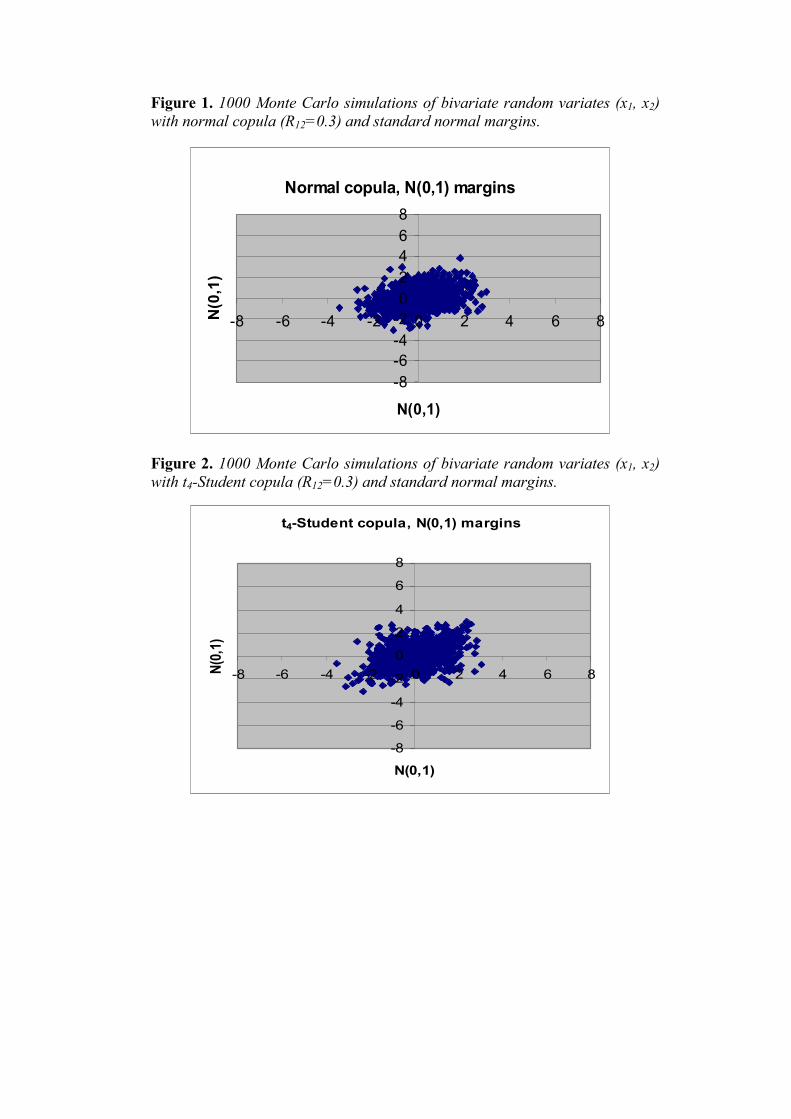
Figure 1. 1000 Monte Carlo simulations of bivariate random variates (x1, x2) with normal copula (R12=0.3) and standard normal margins.

Normal copula, N(0,1) margins

-8-6-4-202468

-8 -6 -4 -2 0 2 4 6 8

N(0,1)

N(0

,1)

Figure 2. 1000 Monte Carlo simulations of bivariate random variates (x1, x2) with t4-Student copula (R12=0.3) and standard normal margins.

t4-Student copula, N(0,1) margins

-8

-6

-4

-2

0

2

4

6

8

-8 -6 -4 -2 0 2 4 6 8

N(0,1)

N(0,

1)

Figure 3. 1000 Monte Carlo simulations of bivariate random variates (x1, x2) with t4-Student copula (R12=0.3) and normalized t4-Student margins.

t4-Student copula, t4-Student margins

-8-6-4-202468

-8 -6 -4 -2 0 2 4 6 8

t4-Student

t4-S

tude

nt

Figure 4. 1000 Monte Carlo simulations of bivariate random variates (x1, x2) with t2-Student copula (R12=0.3) and normalized t2-Student margins.

t2-Student copula, t2-Student margins

-8-6-4-202468

-8 -6 -4 -2 0 2 4 6 8

t2-Student

t2-S

tude

nt

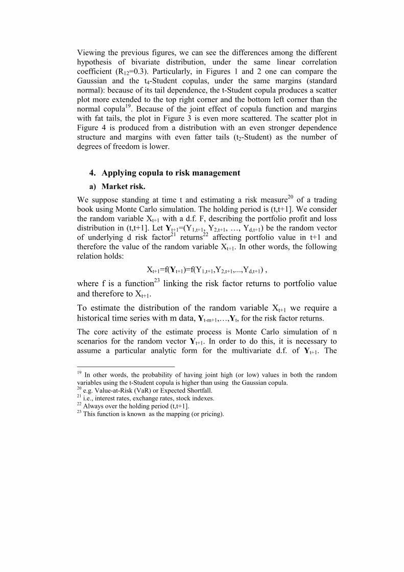
Viewing the previous figures, we can see the differences among the different hypothesis of bivariate distribution, under the same linear correlation coefficient (R12=0.3). Particularly, in Figures 1 and 2 one can compare the Gaussian and the t4-Student copulas, under the same margins (standard normal): because of its tail dependence, the t-Student copula produces a scatter plot more extended to the top right corner and the bottom left corner than the normal copula19. Because of the joint effect of copula function and margins with fat tails, the plot in Figure 3 is even more scattered. The scatter plot in Figure 4 is produced from a distribution with an even stronger dependence structure and margins with even fatter tails (t2-Student) as the number of degrees of freedom is lower.

4. Applying copula to risk management a) Market risk.

We suppose standing at time t and estimating a risk measure20 of a trading book using Monte Carlo simulation. The holding period is (t,t+1]. We consider the random variable Xt+1 with a d.f. F, describing the portfolio profit and loss distribution in (t,t+1]. Let Yt+1=(Y1,t+1, Y2,t+1, …, Yd,t+1) be the random vector of underlying d risk factor21 returns22 affecting portfolio value in t+1 and therefore the value of the random variable Xt+1. In other words, the following relation holds:

Xt+1=f(Yt+1)=f(Y1,t+1,Y2,t+1,...,Yd,t+1) ,

where f is a function23 linking the risk factor returns to portfolio value and therefore to Xt+1. To estimate the distribution of the random variable Xt+1 we require a historical time series with m data, Yt-m+1,…,Yt, for the risk factor returns.

The core activity of the estimate process is Monte Carlo simulation of n scenarios for the random vector Yt+1. In order to do this, it is necessary to assume a particular analytic form for the multivariate d.f. of Yt+1. The

19 In other words, the probability of having joint high (or low) values in both the random variables using the t-Student copula is higher than using the Gaussian copula. 20 e.g. Value-at-Risk (VaR) or Expected Shortfall. 21 i.e., interest rates, exchange rates, stock indexes. 22 Always over the holding period (t,t+1]. 23 This function is known as the mapping (or pricing).

multinormal distribution is a standard assumption in many risk management applications. In fact, such distribution is easy to implement in a simulation model. Unfortunately, empirical evidence proved that the multivariate normal is inadequate because it underestimates both the thickness of the tails of the margins and their dependence structure24.

In our opinion, a more effective model assumes any distributional form for the marginal distributions of Yi,t+1, i=1,…,d, and their dependence structure described by an appropriate copula function. The margins and copula parameters are assessed from historical data.

When we have generated n scenaros for risk factor returns25, we can easily determine n realisations of the random variable Xt+1=f(Yt+1). So we can build the simulated profit and loss distribution. We now have the following options to estimate risk measures (VaR or Expected Shortfall with a given confidence level):

��the n scenarios of Xt+1 are ordered by growing loss values26; VaR is estimated by cutting the simulated distribution at the selected probability level; Expected Shortfall is the expected value of the losses in the worst scenarios27;

��a suitable parametric univariate distribution is fitted to simulated data; VaR and Expected Shortfall are calculated from this distribution;

��estimate the tail distribution of Xt+1 using the superior techniques of Extreme Value Theory and calculate VaR and Expected Shortfall at high confidence level.

b) Credit Risk. The aim is the estimate of credit portfolio risk measures using a latent variable model28 over a time horizon [0,T]29. We consider a portfolio of m

24 i.e., in the case of a market crash, all the stock prices falling down simultaneously. A methodology assuming the multinormal hypothesis does not model effectively such eventuality. 25 n variates of the random vector Yt+1. 26 Profits are assumed as negative losses. 27 The number of worst scenarios derives from the selected probability level. 28 Such kind of models are based on the structural model builds on the pioneering work of Merton (1974). 29 Typically T=1 year.

counterparties. Let the random variable Yi be a default indicator with the following analytical form:

���

�T][0,in defaults ity counterpar if 1

T][0,in default not does ity counterpar if 0iY , i=1, …, m .

The latent variable models use the following pair of vectors to simulate a counterparty default or non default30 over the time horizon [0,T]:

1. let X=(X1,…,Xm) be the random vector of the latent variables. In the Merton approach, such a vector is interpreted as counterparty asset values31 over the time horizon [0,T];

2. let D=(D1,…,Dm) be the deterministic vector of the threshold levels. In the Merton approach, they represent the values of counterparty liabilities32.

The pair (Xi, Di)i=1,…,m denotes a latent variable model for the binary random vector Y=(Y1,…,Ym) if the following relations are true:

iii

ii

DXYDXY

���

���

0 1 1 , i=1,…,m .

The traditional portfolio credit risk models33 implicitly assume a multinormal distribution for the vector X. In some recent academic papers34, it has been stressed how such models can heavily underestimate the probability of many joint defaults and, therefore the whole portfolio risk.

Such a limit is overcome by a model assuming any kind of univariate d.f., Fi, for each component Xi of the vector X, and a copula function (different from the Gaussian copula) describing their dependence structure35.

30 That is if Yi=1 or Yi=0. 31 Since asset returns are not directly observable, CreditMetricsTM of J.P. Morgan chose equity returns as a proxy. 32 In KMVTM, the thresholds represent the values of the short-term debt plus half the long-term debt. 33 i.e., CreditMetrics or KMV. 34 e.g., see Frey and McNeil (2001). 35 e.g. the t-Student copula with a proper number of degrees.

5. Estimating risk measures for a portfolio of Italian equities with copulas

In this section, we perform an application of the model described in section 4a.

We estimate 99% VaR and Expected Shortfall for a portfolio of ten Italian equities36 (d=10) over a one day holding period, using Monte Carlo simulation. We have assessed the model parameters using a four year historical time series37 of the daily closing prices and returns for ten equities (a series of m=1012 data). Table 1 shows the closing prices38 in t, Pit, the expected returns and the return variances. Table 2 shows the empirical asset return correlation matrix39. Portfolio value in t is40:

��

��

10

1Euro 3821,31

iitt PP .

36 See Table 1. 37 From the 25th September 1997 to the 24th September 2001. 38 In Euro. 39 The correlation matrix actually used in the simulations is obtained as follows: the data are mapped to empirical uniforms and transformed with the inverse function of the Gaussian distribution. The correlation is then computed for the transformed data. 40 We consider a portfolio with one unit of each asset.

Table 1. Asset prices in t, expected returns and return variances.

Asset (i) Price, Pit Expected return, ri

Variance, σi2

1 – Banca di Roma 1,95 -0,00024 0,000687

2 – Seat 0,651 0,001215 0,001088

3 – L’Espresso 1,975 0,001112 0,000971

4 – Autostrade 6,05 0,001286 0,000485

5 – AEDES 2,17 0,002933 0,002143

6 – TIM 4,78 0,000602 0,000669

7 – ENI 11,82 0,000218 0,000359

8 - FinMeccanica 0,635 0,000881 0,000855

9 – Olivetti 0,955 0,001406 0,000977

10 - Impregilo 0,3961 -0,00021 0,000539

Table 2. Asset return correlation matrix.

R1 R2 R3 R4 R5 R6 R7 R8 R9 R10

R1 1

R2 0,1968 1

R3 0,2536 0,4929 1

R4 0,3258 0,1864 0,2689 1

R5 0,1233 0,2538 0,2472 0,1353 1

R6 0,3379 0,4345 0,4149 0,3407 0,1858 1

R7 0,3524 0,1222 0,1646 0,2801 0,0716 0,2895 1

R8 0,2900 0,3298 0,3345 0,3026 0,1843 0,3962 0,2187 1

R9 0,3219 0,3888 0,3702 0,2967 0,1630 0,5241 0,1691 0,4002 1

R10 0,3057 0,2000 0,2320 0,3706 0,1293 0,3432 0,2467 0,3658 0,3114 1

We assume standing at time t. We have simulated n=1000 Monte Carlo scenarios for asset returns, Rij, i=1,…,10; j=1,…,1000, over the time horizon (t,t+1] (one day), assuming different analytic forms for the margins and the copula function describing their dependence structure. Using such scenarios, the portfolio has been revalued at time t+1:

��

���

10

11, )1(

iijittj RPP , j=1,…,1000.

We express portfolio losses41 in each scenario j as:

� ��� �

�������

10

1

10

11, )1(

i iijitijitittjt RPRPPPP �

, j=1,…,1000.

So, we obtain the simulated portfolio profit and loss distribution. The calculus of 99% VaR and Expected Shortfall of this distribution is trivial. As already mentioned, such risk measures have been estimated making different hypothesis about the analytic forms of the marginal distribution functions of asset returns and the copula function explaining their dependence structure. The results are shown in Table 3 and compared with 99% VaR and Expected Shortfall obtained from empirical data. The goal is finding the model that better represents empirical evidence.

41 Possibile profits are considered as negative losses.

Table 3. 99% VaR and Expected Shortfall (ES)42 estimated from historical data and from 1000 Monte Carlo (MC) scenarios under different hypotheses of marginal return distributions and their copula.

Empirical distribution (1012 historical scenarios of asset returns) VaR(99%)=1,2809 Euro (4,08%); ES(99%)=1,5662 Euro (4,99%)

1000 MC simulations, normal margins and copula VaR(99%)=1,1213 Euro (3,57%); ES(99%)=1,3127 Euro (4,18%)

Valuation error: VaR -12,46%; ES -16,19%

1000 MC simulations, t50-Student margins and copula VaR(99%)=1,1531 Euro (3,67%); ES(99%)=1,3778 Euro (4,39%)

Valuation error: VaR -9,98%; ES -12,03%

1000 MC simulations, t20-Student margins and copula VaR(99%)=1,2629 Euro (4,02%); ES(99%)=1,5401 Euro (4,91%)

Valuation error: VaR -1,41%; ES -1,67%

1000 MC simulations, t10-Student margins and copula VaR(99%)=1,3022 Euro (4,15%); ES(99%)=1,6478 Euro (5,25%)

Valuation error: VaR +1,66%; ES +5,21%

1000 MC simulations, t4-Student margins and copula VaR(99%)=1,6065 Euro (5,12%); ES(99%)=2,4869 Euro (7,92%)

Valuation error: VaR +25,42%; ES +58,79%

1000 MC simulations, t2-Student margins and copula VaR(99%)=4,2247 Euro (13,46%); ES(99%)=8,6535 Euro (27,57%)

Valuation error: VaR +229,82%; ES +452,52%

From Table 3, we can immediately see that the hypothesis of normal asset return marginal distributions and normal copula, commonly used in risk

42 The per cent ratio between VaR (or Expected Shortfall) and portfolio value is showed in brackets.

management applications, underestimates portfolio 99% VaR and Expected Shortfall calculated with empirical data. Precisely, the VaR underestimate is slightly below 12.5%, while the ES underestimate is above 16%. On the other hand, the hypothesis of t-Student margins and copula, when the number of degrees of freedom is below ten, heavily overestimates portfolio risk. In fact, such a hypothesis produces an excessive overestimate of the tail thickness of profit and loss distribution for a market portfolio, as one can immediately see from Figure 5, 6, 7, and 8.

The hypothesis that better approximate empirical evidence seems to be the t-Student with a number of degrees of freedom between 10 and 20 for the margins and the copula. In fact, in using t20-Student, portfolio VaR and ES are underestimated by about 1.5%, while in using t10-Student there is a slight overestimate of the two risk measures.

Figure 5. Portfolio profit and loss frequency distributions under three different assumptions for asset return marginal distributions and copula function (Gaussian, t4-Student, and t2-Student).

P&L distribution

020406080

100120140160180

-5 -3 -1 1 3 5

Losses

Fre

qu

en

cy

Gaussiant4-Studentt2-Student

Figure 6. Portfolio profit and loss frequency distribution obtained from 1000 MC simulations with Gaussian margins and copula.

P&L distribution

020406080

100120140160180200

-4,9

-4,3

-3,7

-3,1

-2,5

-1,9

-1,3

-0,7

-0,1 0,5 1,1 1,7 2,3 2,9 3,5 4,1 4,7

Losses

Freq

uenc

ies

Gaussian

Figure 7. Portfolio profit and loss frequency distribution obtained from 1000 MC simulations with t4-Student margins and copula.

P&L distribution

020406080

100120140160180

-4,9 -4,1 -3,3 -2,5 -1,7 -0,9 -0,1 0,7 1,5 2,3 3,1 3,9 4,7

Losses

Freq

uenc

ies

t4-Student

Figure 8. Portfolio profit and loss frequency distribution obtained from 1000 MC simulations with t2-Student margins and copula.

P&L distribution

02040

6080

100120

140160180

-4,9

-4,1

-3,3

-2,5 -1,7

-0,9 -0,1 0,7 1,5 2,3 3,1 3,9 4,7

Losses

Freq

uenc

ies

t2-Student

6. An application of copula function to portfolio credit risk measurement

The application in this section has been performed following the model described in section 4b.

We consider a generic portfolio of m=30 loans with exposure values between 31,250 Euro and 88,750 Euro. The total portfolio exposure is 1,607,500 Euro. The 30 loans are classified in 5 different credit states: A, B, C, D, and E. The loans with a better credit worthiness are in credit state A. A loan’s credit worthiness gets worse up to credit state E. We suppose that all the loans in the same credit state have the same yearly probability of default (see Table 4).

Table 4. Credit states and probability of default.

Credit state Probability of default

A 0.8%

B 2.5%

C 5%

D 7,5%

E 15%

The model assumes a constant recovery rate of 0.2 for all the loans.

The latent variables joined to the 30 loans are simulated assuming different analytic forms for the marginal distributions Fi, i=1,2,…,30, and the copula43. The thresholds, Di, i=1,2,…,30, have been calculated inverting the distribution functions of the latent variables in a point equivalent to the probabilty of default of each loan (PDi): Di=Fi

-1(PDi). In this way, the probability that the latent variable value in a scenario falls below the threshold is exactly the probabilty of default of the loan.

The latent variables are simulated assuming a constant linear correlation coefficient of 0.2 between any pair44. The holding period is assumed to be one year.

A scenario is a determination of the vector composed of the 30 latent variables45. A counterparty is in default if its latent variable value, Xi, falls below the threshold, Di. In this case, the loss is equal to the exposure value multiplied by one minus the recovery rate. On the contrary, the counterparty loss is assumed to be zero. Portfolio losses in a scenario are calculated by adding each counterparty loss. Generating n scenarios46, we can easily obtain the portfolio loss distribution. In Figure 9, two different loss distributions, over

43 We have used the Gaussian copula and the t-Student copula with different degrees of freedom. 44 One can observe that 0.2 is the asset correlation value assumed in the new Basle Committee proposal (January 2001) to calculate the risk weight coefficients in the Internal Ratings Based (IRB) approach. Remember that, in the Merton model, the latent variables are the asset returns of any counterparty. 45 One latent variable for each loan (or counterparty). 46 In our application n=1000.

a yearly holding period, are shown. The first is obtained assuming a multinormal distribution for the latent variables47; the second assuming t2-Student margins and copula.

Figure 9. Portfolio loss distributions calculated with 1000 Monte Carlo scenarios under the hypothesis of, respectevely, Gaussian and t2-Student margins and copula for the latent variables.

Loss distribution

0

50

100

150

200

250

300

350

0

1000

00

2000

00

3000

00

4000

00

5000

00

6000

00

7000

00

8000

00

9000

00

1000

000

1100

000

Losses

Freq

uenc

ies

Gaussiant2-Student

47 This is the hypothesis made in most of the common portfolio credit risk internal models.

We can immediately see how the tail of portfolio loss distribution is remarkably longer and fatter under the hypothesis of t2-Student margins and copula of the latent variables. Therefore, the multinormal distribution does not capture extreme risk. Extreme risk in loan portfolios is the risk of many joint defaults over the specified time horizon. On the contrary, events of this kind are effectively captured using the t-Student copula.

In Table 5 we show the values of some portfolio risk measures48. These measures are assessed assuming different analytical forms for the marginal distributions of the latent variables and the copula representing their dependence structure49.

Table 5. Portfolio risk measures (expressed in Euro) assessed with 1000 Monte Carlo scenarios, assuming different hypotheses for the margins and the copula of the latent variables (Gaussian and t-Student with, respectively, 20, 10, 4 and 2 degrees of freedom).

Gaussian t20-Student t10-Student t4-Student t2-Student

EL 71.141 71.180 80.377 107.848 147.707

ML(99%) 349.000 372.500 472.000 615.500 787.500

C-VaR(99%) 277.858 301.320 391.622 507.651 639.792

ES(99%) 433.150 464.250 556.500 783.250 936.050

We can immediately see that tail risk measures (ML, C-VaR and ES) are drastically higher under the t2-Student hypothesis than under the Gaussian hypothesis. In fact, the normal copula does not have tail dependence and so it is not able to capture the event of many joint counterparty defaults. Unfortunately, it is just this kind of event that worries bank risk managers and supervisors. From this point of view, a model based on the t-Student copula is more effective. 48 That is the Expected Loss (EL), 99% Maximum Loss (ML), 99% Credit-VaR (C-VaR), and 99% Expected Shortfall (ES). We remember that Credit-VaR is the Maximum Loss, that is a quantile of loss distribution, minus the Expected Loss. 49 It is an extension of the application developed in Frey and McNeil (2001). They determined the distribution of the number of joint counterparty defaults. All the counterparties belonged to the same credit state.

Concluding remarks In this work we have described some possible uses of copula functions in risk management applications. Copula function represents the dependence structure of a random variable vector. For instance, these random variables stand for the asset returns of a portfolio over a specified time horizon. We have proved how some kind of copula functions50 are easy to implement in Monte Carlo simulation models to estimate risk measures.

We have performed a practical application with a portfolio of ten Italian equities. We have proved that the common hypothesis of multinormal distribution for asset returns (or risk factor returns) underestimates the VaR and the Expected Shortfall of a market portfolio. We have performed a Monte Carlo simulation, modelling asset returns using fat tail marginal distributions and a copula function with tail dependence51. In this way, we have obtained a more accurate estimate for the two risk measures.

We have also presented an application of copula function to model portfolio credit risk. We have proved that a methodology using a multivariate Gaussian distribution of the latent variables52 does not capture the risk of many joint counterparty defaults. On the contrary, events of this kind are effectively captured using the t-Student copula to describe the dependence structure of the latent variables. Therefore, the t-Student copula can be very useful to model the extreme risk that worries risk managers and supervisors.

50 Precisely the elliptical copulas. 51 The t-Student copula. 52 CreditMetrics and KMV use this hypothesis.

References - Bouyé, E., V. Durrleman, A. Nikeghbali, G. Riboulet and T. Roncalli (2000): “Copulas for finance – a reading guide and some applications”, Groupe de Recherche Opérationnelle, Crédit Lyonnais, Working Paper.

- Bouyé, E., V. Durrleman, A. Nikeghbali, G. Riboulet and T. Roncalli (2001): “Copulas: an open field for risk management”, Groupe de Recherche Opérationnelle, Crédit Lyonnais, Working Paper.

- Embrechts, P., A. Hoeing and A. Juri (2001): “Using copulae to bound the Value-at-Risk for functions of dependent risks”, ETH Zurich, preprint.

- Embrechts, P., F. Lindskog and A. J. McNeil (2001): “Modelling dependence with copulas and applications to risk management”, ETH Zurich, preprint.

- Embrechts, P., A. J. McNeil and D. Straumann (1999): “Correlation and Dependence in Risk Management: Properties and Pitfalls”, To appear in Risk Management: Value at Risk and Beyond, ed. By M. Dempster and H. K. Moffatt, Cambridge University Press.

- Frey, R. and A. J. McNeil (2001): “Modelling dependent default”, ETH Zurich preprint.

- Li, D. (1999): “On Default Correlation: A Copula Function Approach”, working paper, RiskMetrics Group, New York.

- Lindskog, F. (2000): “Modelling Dependence with Copulas”, ETH Zurich.

- Merton, R. (1974): “On the Pricing of Corporate Debt: The Risk Structure of Interest Rates”, Journal of Finance, 29, pp. 449-470.

- Nelsen, R. (1999): “An Introduction to Copulas”, Springer, New York.

- Sklar, A. (1959): “Fonctions de répartition à n dimensions et leurs marges", Publications de l’Institut de Statistique de l’Université de Paris, 8, pp. 229-231.

- Sklar, A. (1996): «Random variables, distribution functions, and copulas – a personal look backward and forward”, in Distributions with Fixed Marginals and Related Topics, ed. By L. Rüschendorff, B. Schweizer and M. Taylor, pp. 1-14. Institute of Mathematical Statistics, Hayward, CA.