UNLV Theses, Dissertations, Professional Papers, and Capstones

August 2019

Applied Symmetry for Crystal Structure Prediction Applied Symmetry for Crystal Structure Prediction

Scott William Fredericks

Follow this and additional works at: https://digitalscholarship.unlv.edu/thesesdissertations

Part of the Condensed Matter Physics Commons, and the Other Physics Commons

Repository Citation Repository Citation Fredericks, Scott William, "Applied Symmetry for Crystal Structure Prediction" (2019). UNLV Theses, Dissertations, Professional Papers, and Capstones. 3723. http://dx.doi.org/10.34917/16076263

This Thesis is protected by copyright and/or related rights. It has been brought to you by Digital Scholarship@UNLV with permission from the rights-holder(s). You are free to use this Thesis in any way that is permitted by the copyright and related rights legislation that applies to your use. For other uses you need to obtain permission from the rights-holder(s) directly, unless additional rights are indicated by a Creative Commons license in the record and/or on the work itself. This Thesis has been accepted for inclusion in UNLV Theses, Dissertations, Professional Papers, and Capstones by an authorized administrator of Digital Scholarship@UNLV. For more information, please contact digitalscholarship@unlv.edu.

APPLIED SYMMETRY FOR CRYSTAL STRUCTURE PREDICTION

By

Scott Fredericks

Bachelor of Science in Physics University of Arkansas, Fayetteville

2011

A thesis submitted in partial fulfillment of the requirements for the

Master of Science - Physics

Department of Physics and Astronomy College of Sciences

The Graduate College

University of Nevada, Las Vegas August 2019

c© Scott Fredericks, 2019

All Rights Reserved

ii

Thesis Approval

The Graduate College

The University of Nevada, Las Vegas

July 10, 2019

This thesis prepared by

Scott Fredericks

entitled

Applied Symmetry for Crystal Structure Prediction

is approved in partial fulfillment of the requirements for the degree of

Master of Science - Physics

Department of Physics and Astronomy

Qiang Zhu, Ph.D. Kathryn Hausbeck Korgan, Ph.D. Examination Committee Chair Graduate College Dean

Ashkan Salamat, Ph.D. Examination Committee Member

Tao Pang, Ph.D. Examination Committee Member

Hui Zhao, Ph.D. Graduate College Faculty Representative

Abstract

This thesis presents an original open-source Python package called PyXtal (pronounced “pi-crystal”)

that generates random symmetric crystal structures for use in crystal structure prediction (CSP).

The primary advantage of PyXtal over existing structure generation tools is its unique symmetriza-

tion method. For molecular structures, PyXtal uses an original algorithm to determine the compat-

ibility of molecular point group symmetry with Wyckoff site symmetry. This allows the molecules in

generated structures to occupy special Wyckoff positions without breaking the structure’s symme-

try. This is a new feature which increases the space of search-able structures and in turn improves

CSP performance.

It is shown that using already-symmetric initial structures results in a higher probability of

finding the lowest-energy structure. Ultimately, this lowers the computational time needed for

CSP. Structures can be generated for any symmetry group of 0, 1, 2, or 3 dimensions of periodicity.

Either atoms or rigid molecules may be used as building blocks. The generated structures can be

optimized with VASP, LAMMPS, or other computational tools. Additional options are provided

for the lattice and inter-atomic distance constraints. Results for carbon and silicon crystals, water

ice crystals, and molybdenum clusters are presented as usage examples.

iii

Acknowledgements

I would first like to thank my advisor, Dr. Qiang Zhu, for his help in completing this Masters

program. I sincerely appreciate his guidance and understanding, and his willingness to take me

on as a student. I’d like to thank my good friends Piyush and David for their friendship, and for

making these two years more enjoyable. Finally, I’d like to thank my mother and sister for their

continued love and support.

Scott Fredericks

University of Nevada, Las Vegas

August 2019

iv

Table of Contents

Abstract iii

Acknowledgements iv

Table of Contents v

List of Figures vii

Chapter 1 Introduction: Crystal Structure Prediction and PyXtal 1

Chapter 2 Background: Symmetry of Atomic Structures 3

2.1 Transformation Operations . . . . . . . . . . . . . . . . . . . . . . . . . . . . . . 3

2.2 Symmetry Operations . . . . . . . . . . . . . . . . . . . . . . . . . . . . . . . . . 4

2.3 Periodic Symmetry . . . . . . . . . . . . . . . . . . . . . . . . . . . . . . . . . . . 4

2.4 Point Group Symmetry . . . . . . . . . . . . . . . . . . . . . . . . . . . . . . . . 5

2.5 Symmetry Groups in Three Dimensions . . . . . . . . . . . . . . . . . . . . . . 6

2.6 Wyckoff Positions . . . . . . . . . . . . . . . . . . . . . . . . . . . . . . . . . . . . 6

2.7 Fractional Coordinates and Periodic Boundary Conditions . . . . . . . . . . 9

2.8 Computer Representations of Symmetry Information . . . . . . . . . . . . . 9

Chapter 3 The Structure Generation Algorithm 12

3.1 Overview . . . . . . . . . . . . . . . . . . . . . . . . . . . . . . . . . . . . . . . . . . 12

3.2 Wyckoff Compatibility Checking . . . . . . . . . . . . . . . . . . . . . . . . . . 12

3.3 Lattice Generation . . . . . . . . . . . . . . . . . . . . . . . . . . . . . . . . . . . 14

3.4 Wyckoff Position Selection and Merging . . . . . . . . . . . . . . . . . . . . . . 14

3.5 Distance Checking . . . . . . . . . . . . . . . . . . . . . . . . . . . . . . . . . . . . 16

3.6 Molecular Orientations . . . . . . . . . . . . . . . . . . . . . . . . . . . . . . . . . 19

v

Chapter 4 Results 21

4.1 Point group clusters . . . . . . . . . . . . . . . . . . . . . . . . . . . . . . . . . . . 21

4.2 Carbon and Silicon Crystals . . . . . . . . . . . . . . . . . . . . . . . . . . . . . 22

4.3 3D Ice . . . . . . . . . . . . . . . . . . . . . . . . . . . . . . . . . . . . . . . . . . . 28

Chapter 5 Comparison with Existing Tools 31

Chapter 6 Limitations and Further Study 33

6.1 Crystal Structure Prediction Methods Used . . . . . . . . . . . . . . . . . . . 33

6.2 Complexity of the Systems Studied . . . . . . . . . . . . . . . . . . . . . . . . . 33

6.3 Molecular Flexibility . . . . . . . . . . . . . . . . . . . . . . . . . . . . . . . . . . 34

6.4 Non-crystalline Systems . . . . . . . . . . . . . . . . . . . . . . . . . . . . . . . . 34

Chapter 7 Conclusion 36

Appendix A LAMMPS Settings Used for H2O 37

Appendix B VASP INCAR for DFT Optimization Step 1 38

Appendix C VASP INCAR for DFT Optimization Step 2 39

Appendix D VASP INCAR for DFT Single Point Energy Calculations 40

Bibliography 41

Curriculum Vitae 45

vi

List of Figures

2.1: Unit Cell Example . . . . . . . . . . . . . . . . . . . . . . . . . . . . . . . . . . . . . 5

2.2: Wyckoff Positions of the Square Group 4mm . . . . . . . . . . . . . . . . . . . . . . 7

2.3: Orientations of Water in a Wyckoff Position . . . . . . . . . . . . . . . . . . . . . . . 8

3.1: PyXtal Structure Generation Flowchart . . . . . . . . . . . . . . . . . . . . . . . . . 13

3.2: Wyckoff Position Merging Example . . . . . . . . . . . . . . . . . . . . . . . . . . . . 15

3.3: Distorted Unit Cell . . . . . . . . . . . . . . . . . . . . . . . . . . . . . . . . . . . . . 17

3.4: Dependence of Shortest Distances on Molecular Orientation . . . . . . . . . . . . . . 18

4.1: Energy distribution for Lennard Jones size 38 Clusters . . . . . . . . . . . . . . . . . 22

4.2: Energy distribution for Lennard Jones size 55 Clusters . . . . . . . . . . . . . . . . . 23

4.3: Energy distribution for Lennard Jones size 75 Clusters . . . . . . . . . . . . . . . . . 23

4.4: Representative Carbon Structures . . . . . . . . . . . . . . . . . . . . . . . . . . . . 24

4.5: Representative Silicon Structures . . . . . . . . . . . . . . . . . . . . . . . . . . . . . 25

4.6: Lattice Energy Distributions for Carbon and Silicon . . . . . . . . . . . . . . . . . . 26

4.7: Representative Ice Structures . . . . . . . . . . . . . . . . . . . . . . . . . . . . . . . 28

4.8: Energy Distribution for H2O Crystals . . . . . . . . . . . . . . . . . . . . . . . . . . 29

vii

Chapter 1

Introduction: Crystal Structure

Prediction and PyXtal

The key to understanding a material’s properties lies in its atomic structure. If the structure is

known, then almost any property can be ascertained through simulation, calculation, or some other

method. In some cases the structure can be determined through experimental techniques such as

X-ray diffraction or Raman spectroscopy [1]. However, this can be a costly and time-consuming

process, and researchers may not have access to the necessary equipment. Furthermore, it is often

impossible to perform experiments on materials which have yet to be synthesized, or which only

exist at extremely high pressures and/or temperatures. The modern solution to this problem is

Crystal Structure Prediction (CSP). The basic idea of CSP is to guess the correct crystal structure

for specific conditions by computationally sampling a wide range of possible structures. After many

attempts, the most energetically stable structure found is the one most likely to exist.

Using CSP, it is possible to discover new materials which have not yet been created. As the

number of known materials grows, scientists and engineers gain new options for implementing new

physical phenomena. For example, the discovery of the photovoltaic effect allowed the invention

of solar-powered electricity. But in order to work, the electrons in a solar cell must be able to

gain an energy level when exposed to sunlight. In practice, this means the material used must

have specific electronic properties, and different materials will produce different results. For any

given application there is a trade off between properties, so there is often no single ideal material.

Thus, the discovery of new materials has the potential to reduce costs and improve performance in

multiple industries. As a result, CSP is a growing field of active research.

1

A typical CSP algorithm works as follows: First, a set of random structures is generated.

Different constraints can be applied (regarding the stoichiometry, lattice, symmetry, etc.) which

limit the search space. Next, the structures are optimized for low energy. This involves calculating

the inter-atomic forces within the crystal, then iteratively relaxing the structure until the forces

cancel out. Simple force-field models are easier to calculate, but produce less accurate results. More

advanced techniques like Density Functional Theory (DFT) take much longer, but in return give

higher physical accuracy. After many generations, the lowest-energy structure is likely to be found,

at least in theory. Further global optimization techniques such as genetic algorithms and machine

learning can also be used to speed up the process [2].

While CSP is generally faster than experimental trial and error, it is still computationally

expensive. Improvements at any step in the process have the potential to significantly cut costs

and to allow more materials to be discovered. To this end, the author has co-developed (with his

advisor Dr. Qiang Zhu) an open-source Python package called PyXtal to handle the structure

generation step.

It has been shown [3] that by beginning with already-symmetric structures, fewer attempts are

needed to find the global energy minimum. In PyXtal, the symmetry constraints are further refined

in two main ways. The first is a merging algorithm [4] which controls the distribution of Wyckoff

positions through statistical means. The second is a new algorithm for placing molecules into

special Wyckoff positions. This allows for more realistic and complex structures to be generated

without reducing the global symmetry.

PyXtal is not a complete CSP package; it only generates the initial structures with a given

symmetry group. Other tools exist which perform structure generation and other steps in the CSP

process. The main goals in developing PyXtal were: 1) to handle molecular Wyckoff positions

in a generalized manner, 2) to demonstrate that proper symmetry considerations lead to better

predictive results, and 3) to develop a free, open-source Python package for the materials science

community.

Access to the source code and development information are available on the GitHub page at

https://github.com/qzhu2017/PyXtal

2

Chapter 2

Background: Symmetry of Atomic

Structures

2.1 Transformation Operations

Crystals are primarily categorized by their spatial symmetry. Mathematically, an object’s symmetry

is the group of transformations which leave its geometric structure invariant. For atomic structures,

the transformations in question are those of 3D space itself: translations, rotations, and inversion.

Collectively, these are called orthogonal transformations. All of these transformations preserve

angles and lengths. With the exception of inversion, all can be physically applied by simply moving

the structure around in real space.

When a transformation operation is applied repeatedly, the final result is sometimes the identity

operation. That is, the object’s final state is the same as its original state. The number of

times an operation must be applied to obtain the identity is called its order. For example, the

identity operation has order 1, reflections have order 2, and rational rotations have integer order.

A randomly chosen transformation will probably never return the object to its original state; thus

such an operation is said to have infinite order.

Because any combination of orthogonal transformations results in another orthogonal transfor-

mation, the set of all orthogonal transformations forms a mathematical group called the orthogonal

group. The tools of group theory simplify the study of transformations and symmetry, as they allow

for concise notation and calculations [5].

3

2.2 Symmetry Operations

Sometimes, applying a transformation will cause no detectable change to an object. Such a trans-

formation is called a symmetry operation. For example, if you rotate a cube by 90 degrees about

one of its faces, it will look the same; thus the 90 degree rotation is called a symmetry operation

of the cube.

Any given object will have some set of symmetry operations. Because symmetry operations

leave the object unchanged, that set is actually a group. This is called the object’s symmetry

group, and is a subgroup of the orthogonal group.

When speaking of symmetry, it is important to clearly define what constitutes equivalence

between objects. In reality, two atoms may or may not be considered distinguishable based on their

spin and other properties. Typically in crystallography, atoms of the same species with structurally

identical environments are treated as indistinguishable. This means that if a transformation maps

every atom onto another atom of the same species, that transformation is considered a symmetry

operation, and the structure is effectively unchanged [6].

2.3 Periodic Symmetry

The defining feature of a crystal is the presence of periodic symmetry. This means that certain

translation vectors, when applied, leave the crystal structure unchanged. For a 3D crystal, one

could choose 3 such vectors. If these vectors are linearly independent, they are known as lattice

vectors, and they form a parallelepiped-shaped substructure called the unit cell. The contents of

a unit cell can be repeatedly “tiled” along its lattice vectors in order to reproduce the rest of the

crystal (see figure 2.1).

The choice of a unit cell is not unique. Given some unit cell, one can arbitrarily choose 3 new

vectors from linear combinations of the original lattice vectors. If the new vectors are again linearly

independent, they will form a new unit cell. Thus there are an infinite number of possible unit

cell choices. Additionally, it is possible to choose any point in the structure as the origin. For

certain space groups, particularly those with multiple centers of inversion symmetry, there is no

single “preferred” choice of origin. But typically, the origin will fall on the location of an atom or

symmetry element. This makes the specification of the symmetry operations simpler.

Nevertheless, certain cell choices are more convenient than others. Because a different choice

of unit cell will result in a different description for the structure, crystallographers have developed

4

(a) (b)

Figure 2.1: Unit Cell Example. a) The unit cell of a randomly generated methane crystal. b) a2x2x2 supercell created by copying and translating the original unit cell along its 3 axes.

a set of standard “conventional” unit cell choices. These are the choices used by PyXtal, and are

outlined in the International Tables of Crystallography, section 2.1.1 [7].

2.4 Point Group Symmetry

Crystals may also possess point group symmetry. The relevant operations are represented by or-

thogonal 3x3 matrices. If a matrix has determinant 1, then the operation is purely rotational,

whereas a matrix with determinant -1 also involves the application of inversion. Such transfor-

mations are called roto-inversions. A symmetry group containing only rotations, reflections, and

inversions is called a point group, because it always leaves at least one point in 3D space unmoved.

Because molecules are finite in size and have a well-defined position, they can possess no trans-

lational symmetry. Thus, point groups are used for studying molecular symmetry and structure.

Because a rotation can have arbitrary or infinite order, there are an infinite number of point

groups. However, most of them are not relevant for crystallography or chemistry. PyXtal has 56

pre-generated point groups which can be chosen for cluster generation. Any other point group can

be specified and generated on the fly using its Schoenflies symbol.

5

2.5 Symmetry Groups in Three Dimensions

A symmetry group can be artificially divided into its translational part (called the t-subgroup)

and its roto-inversional component (the point group, or k-subgroup). Because a lattice is not

always invariant under rotations, not every point group can be found in objects with translational

symmetry. For the 3D case, there are only 32 point groups which are compatible with a lattice.

These are called the crystallographic point groups, and every crystal possesses one of these as its

k-subgroup.

In accordance with the crystallographic restriction theorem [8], 3D crystals may only possess

1, 2, 3, 4, or 6-fold rotational symmetry. Other orders of rotation are not compatible with 3

dimensions of periodicity. However, 5-fold symmetry has been observed in the diffraction pattern

of quasicrystals [9]. These structures do not possess exact translational symmetry, but still have

some long-range order. The description of such structures deviates from standard group theory, and

is thus beyond the scope of PyXtal. However, some tools do exist for the analysis of quasicrystals

[10].

If a symmetry group includes 3D lattice symmetry, it is called a space group. Groups with only

2 lattice vectors are called layer groups, and groups with 1 lattice vector are called Rod groups.

There are 230 unique space groups, 80 layer groups, and 75 Rod groups. These, along with point

groups, are the symmetry groups used by PyXtal for generating structures.

2.6 Wyckoff Positions

When the operations of a symmetry group are applied to a randomly chosen atomic position, that

atom can be thought of as being repeated in space. This results in a number of copies equal to the

order of the symmetry group. The generated set of atoms is then symmetric under the operation

which was applied.

However, point group operations always map certain positions back onto themselves. This

high-symmetry location can be a point, line, plane, or 3D space (3D space occurring only for the

identity operation), and is called the symmetry element of the operation. As a result, atoms lying

on symmetry elements will be mapped back onto themselves, and will thus not be copied by every

operation. The symmetrically unique symmetry elements of a symmetry group are called Wyckoff

positions (WP’s). A WP which includes all of space is called the general position; all others are

called special Wyckoff Positions [11].

6

The term “Wyckoff position” refers not necessarily to a single point, but to a set of points

generated by the symmetry group. As an example, the space group Pmmm has order 8. Its general

WP contains 8 atoms, but these 8 atoms are collectively referred to as a single WP (see figure

2.2). Furthermore, because each point in the WP is symmetrically equivalent, one can refer to the

entire position using only a single coordinate. The number of symmetrically equivalent points in

a Wyckoff position is called its multiplicity. WP’s reduce the amount of information needed to

describe a crystal, provided the symmetry group is known. The CIF (Crystallographic Information

File) file format uses this method and only stores one atom per Wyckoff position, while the POSCAR

file format (used by VASP) stores each atom separately [12] [13]. As a result, CIF files tend to be

smaller than POSCAR files for crystals with large unit cells. On the other hand, reading from the

CIF format requires the generation of the remaining points using the symmetry group information.

This exemplifies an inherent trade-off in the representation of symmetric information.

8c (1)

4b (..m)

4a (.m.)

1o (4mm)

Wyckoff positions of the 2D Point

Group 4mm

Figure 2.2: Wyckoff Positions of the Square Group 4mm. The 2D point group 4mm contains allplanar symmetries of the square. Here, the solid and dashed lines mark the 4 reflectional symmetryelements. Present but not marked is a 4-fold rotational symmetry about the center. The differentshapes are examples of objects in the 4 Wyckoff positions 8c, 4b, 4a, and 1o, with 8c being thegeneral position. Different shapes of the same kind belong to a single Wyckoff position.

The subgroup of operations which maps a WP onto itself is called its site symmetry. For atomic

crystals, a WP’s site symmetry only determines which 3D positions an atom can lie within. For

7

molecular crystals, however, the site symmetry also limits which kinds of molecules can lie within

certain WP’s. For example, if a WP has site symmetry 2/m (a two-fold rotation accompanied by a

reflection), then any molecule in that position must also have 2/m as a subgroup of its point group.

Additionally, the molecule must be oriented in such a way that its relevant symmetry axes are in

the same orientation as the symmetry axes of the WP (see figure ??).

(a) (b) (c)

(d) (e) (f)

Figure 2.3: Orientations of Water in a Wyckoff Position. The planes and non-pointed axes representthe symmetry elements of a Wyckoff position with site symmetry mm2. Each plane represents areflectional symmetry, and the blue-ringed axis represents a 2-fold rotational symmetry. (a) a watermolecule with random orientation, (b) the water molecule after its rotation symmetry axis (blue,pointed) is aligned with the corresponding site symmetry rotation element, (c) the water moleculeafter one of its reflectional axes (green, pointed) is aligned with the corresponding site symmetryreflection element, (d)-(f) the 3 remaining valid and unique molecular orientations.

Every symmetry group has a unique set of WP’s. To refer to a specific WP within a group,

crystallographers use both a letter (called the Wyckoff letter) and the multiplicity. The letter

increases alphabetically as the multiplicity goes up. Common examples of WP names include 1a,

2b, 4e, or 8g, but different groups will have different names for their WP’s. It is worth noting

that a different choice of unit cell or origin can result in different descriptions of the WP’s as well.

Typically, the letter-number combination refers to a WP in a standard conventional space group

8

setting.

In a sense, all of the information about a group is stored in its WP’s. In fact, a structure with

a given symmetry group can be thought of as a collection of WP’s with different objects in them.

This is precisely the approach used by PyXtal for structure generation. If atoms are only allowed to

exist in a group’s WP’s, then the resulting structure is guaranteed to have that group’s symmetry,

regardless of how many atoms are added.

2.7 Fractional Coordinates and Periodic Boundary Conditions

When working with atomic positions in a crystal, it is common to use a coordinate system based

on the unit cell, rather than Euclidean space. Such coordinates are called fractional coordinates.

For example, the fractional coordinate (0.0, 0.25, 0.5) would lie on the 0-plane of the a-axis, 1/4 of

the way along the b-axis, and 1/2 of the way along the c-axis. The Euclidean coordinates would

depend on the shape of the lattice.

Because crystals are periodic along integer translations of their unit cell axes, a single frac-

tional coordinate actually refers to an infinite lattice of equivalent points. For most purposes, any

fractional coordinate less than 0 or greater than 1 will be translated by integer values until it lies

between (0,0,0) and (1,1,1).

When working with crystals computationally, it is important to remember that any object

within the unit cell is actually an infinite lattice of equivalent objects. This is especially relevant

for distance calculations, as discussed in later sections.

2.8 Computer Representations of Symmetry Information

Any orthogonal transformation can be described by the combination of a 3x3 orthogonal matrix

(which describes the orientation) and a 3-vector (which describes the translation). One can trans-

form a 3-vector (x, y, z) into a new vector (x’, y’, z’) by first applying a rotation matrix M, and

then adding a translation vector v:

M11 M12 M13

M21 M22 M23

M31 M32 M33

x

y

z

+

v1

v2

v3

=

x′

y′

z′

9

However, one can simplify this operation by representing the transformation and the original

3-vector using “augmented” 4x4 matrices [14]. Here, the 3x3 matrix and 3x1 vector are placed into

a single 4x4 matrix, with 0’s and a 1 on the bottom row:

M11 M12 M13

M21 M22 M23

M31 M32 M33

,v1

v2

v3

→M11 M12 M13 v1

M21 M22 M23 v2

M31 M32 M33 v3

0 0 0 1

With this notation, it becomes clear that one must define both orientation and position. But

as a result, operations can be applied using standard matrix multiplication:

M11 M12 M13 v1

M21 M22 M23 v2

M31 M32 M33 v3

0 0 0 1

O11 O12 O13 x

O21 O22 O23 y

O31 O32 O33 z

0 0 0 1

=

O′

11 O′12 O′

13 x′

O′21 O′

22 O′23 y′

O′31 O′

32 O′33 z′

0 0 0 1

Here, the 3x3 matrix O represents the original orientation of the object being transformed, and

O’ is the new orientation.

For symmetric objects, orientations are ambiguous by definition. Atoms, which are assumed

to be spherically symmetric, do not have a well-defined orientation, because there is no way to

distinguish which way an atom is “facing”. More generally, a single orientation for a symmetric

object actually corresponds to a group of orientations which is conjugate to the object’s symmetry

group.

For example, consider an object with reflection symmetry. If a random orientation is chosen,

then there is always one other orientation (the mirror image) which is indistinguishable from the

original orientation. Thus, the number of unique orientations is half as large as it would be for

an asymmetric object. In general, as the symmetry group grows, the space of unique orientations

shrinks. A group-theoretic representation of orientation would thus use a different size of object

depending on the size of the symmetry group. Indeed, in quantum mechanics the symmetry of

particles directly influences their statistical behavior. A well-known example is that the number of

degrees of freedom for a molecule changes its thermodynamic properties.

10

For PyXtal’s purposes, it suffices to simply store an object’s orientation matrix and its symmetry

operations. Comparisons between orientations can still be performed algorithmically this way.

In certain cases, particularly when using special Wyckoff positions, one may want to apply

singular transformations. For example, one may want to place a randomly located atom into the

Wyckoff position (0,0,z). In this case, the position is effectively 1-dimensional, despite existing

within 3D space. The solution is to project the original coordinate onto the symmetry element

represented by the Wyckoff operator.

As another example, consider the symmetry element (x,x,0), which is a diagonal axis running

through the z-plane. If the original point were (0.9,0.1,0.0), then the projected point on the axis

would be (0,0,0) due to periodic boundary conditions.

In practice, coordinates can be generated for any Wyckoff position by simply applying the

Wyckoff position’s 4x4 matrices to an arbitrary 3-vector. However, to ensure an even distribution

of points in 3D space, one must first find the closest projection of the point onto the symmetry

element. So, a Wyckoff position can be thought of as a set of 4x4 matrices, and a space group can

be thought of as a set of Wyckoff positions. The storage, interpretation, and arithmetic for the 4x4

matrices is currently handled by Pymatgen’s SymmOp class [15].

Because non-integer matrix multiplication depends on floating point operations, numerical ac-

curacy is a legitimate concern. To check for equivalence, it is useful to define some cutoff difference

tolerance. If all matrix values are equal within this tolerance, then matrices are considered equal.

Because PyXtal only works with groups of order less than a few hundred, this accuracy is sufficient.

For groups of very high order, one might instead use quaternions or other calculation methods with

higher numerical accuracy.

11

Chapter 3

The Structure Generation Algorithm

3.1 Overview

PyXtal follows the same basic algorithm for each type of structure which can be generated. First,

the user inputs their choice of dimension (0, 1, 2, or 3), symmetry group, stoichiometry, and rel-

ative volume of the unit cell. Optionally, additional parameters may be chosen which constrain

the unit cell and maximum inter-atomic distance tolerances. This is implemented through the

random crystal and molecular crystal Python classes. Next, PyXtal checks to make sure the stoi-

chiometry is compatible with the choice of symmetry group. If the check passes, then generation

begins. Figure 3.1 shows a flowchart of the algorithm.

Each remaining step has a maximum number of attempts. If generation fails at any point,

the algorithm will revert progress for the current step and try again, until the maximum attempt

limit has been reached. This ensures that the algorithm stops in finite time, while still giving each

generated parameter a chance for success. For certain inputs, generation may take many attempts

or fail after the maximum number of attempts. Typically, these failures indicate that the input

parameters are not likely to produce a realistic structure without fine-tuned atomic positions. In

such cases, a larger unit cell or smaller distance tolerances may improve the chances of successful

generation.

3.2 Wyckoff Compatibility Checking

Before attempting to generate a structure, PyXtal must make sure it is possible to do so. The

WP’s in different space groups have different multiplicities. As a result, not every number of atoms

is compatible with every space group. For example, consider the space group Pn-3n (#222). The

12

Figure 3.1: PyXtal Structure Generation Flowchart. Generation is based on inputs from the user.

smallest Wyckoff position is 2a, with the next smallest being 6b. It is impossible to create a crystal

with 4 atoms in the unit cell for this symmetry group, because no combination of Wyckoff positions

adds up to 4. The position 2a cannot be repeated, because it falls on the exact coordinates (1/4,

1/4, 1/4) and (3/4, 3/4, 3/4). A second set of atoms in the 2a position would overlap the atoms

in the first position, but this is not physically possible.

Thus, it is necessary to check the input stoichiometry against the Wyckoff positions of the

desired space group. To accomplish this, PyXtal iterates through all possible Wyckoff position

combinations within the confines of the stoichiometry. As soon as one valid combination is found,

the check returns true. If no valid combination is found, the check returns false, and the generation

attempt fails with a warning.

Some space groups allow valid combinations of WP’s, but may not give many degrees of freedom

for generation. It may also be the case that the allowed combinations result in atoms which are

too close together. In these cases, PyXtal will attempt generation as usual: until the maximum

limit is reached, or until a successful generation occurs. If generation repeatedly fails for a given

combination of space group and stoichiometry, the user should make note and avoid the combination

going forward.

13

3.3 Lattice Generation

The first step in PyXtal’s structure generation is the choice of unit cell. Depending on the symmetry

group, a specific type of lattice must be generated. For all crystals, the conventional cell choice is

used to avoid ambiguity. The most general case is the triclinic cell, from which other cell types can

be obtained by applying various constraints.

To generate a triclinic cell, 3 real numbers are randomly chosen (using a Gaussian distribution

centered at 0) as the off-diagonal values for a 3x3 shear matrix. Treating this matrix as a cell

matrix, one obtains 3 lattice angles. For the lattice vector lengths, a random 3-vector between

(0,0,0) and (1,1,1) is chosen (using a Gaussian distribution centered at (0.5,0.5,0.5)). The relative

values of the x, y, and z coordinates are used for a, b, and c respectively, and scaled based on the

required volume.

For other cell types, any free parameters are obtained using the same methods as for the triclinic

case, along with any necessary constraints. In the tetragonal case, for example, all angles must be

90 degrees. Thus, only a random vector is needed to generate the lattice constants.

3.4 Wyckoff Position Selection and Merging

The central building block for crystals in PyXtal is the Wyckoff position (WP). Once a space group

and lattice are chosen, WP’s are inserted one at a time to add structure.

PyXtal starts with the largest available WP, which is the general position of the space group.

If the number of atoms required is equal to or greater than the size of the general position, the

algorithm proceeds. If fewer atoms are needed, the next largest WP (or set of WP’s) is chosen,

in order of descending multiplicity. This is done to ensure that larger positions are preferred over

smaller ones; this reflects the greater prevalence of larger multiplicities both statistically and in

nature.

Once a WP is chosen, a random 3-vector between (0,0,0) and (1,1,1) is created. This acts as

the generating point. Projecting this vector into the WP, one obtains a set of coordinates in real

space. Then, the distances between these coordinates are checked. If the atom-atom distances

are all greater than a pre-defined limit, the WP is kept and the algorithm continues. If any of

the distances are too small, it is an indication that the WP would not occur with that generating

point. In this case, the coordinates are merged together into a smaller WP, if possible. This merging

continues until the atoms are no longer too close together (see figure 3.2).

14

To merge into a smaller position, the original generating point is projected into each of the

remaining WP’s. The WP with the smallest translation between the original point and the trans-

formed point is chosen, so long as the new WP is a subset of the original one, and so long as the

new points are not too close together. If the atoms are still too close together, the WP is discarded

and another attempt is made.

8c 4a

4b 1o

Figure 3.2: Wyckoff Position Merging Example. Shown are possible mergings of the general position8c of the 2D point group 4mm. Moving from 8c to 4b (along the solid arrows) requires a smallertranslation than for 4a (along the dashed arrows). Thus, if the atoms in 8c were too close together,PyXtal would merge them into 4b instead of 4a. The atoms could be further merged into position1o by following the arrows shown in the bottom right image.

Once a satisfactory WP has been filled, the inter-atomic distances between the current WP and

the already-added WP’s are checked. If all distances are acceptable, the algorithm continues. More

WP’s are then added as needed until the desired number of atoms has been reached. At this point,

either a satisfactory structure has been generated, or the generation has failed. If the generation

15

fails, then either smaller distances tolerances or a larger volume factor might increase the chances

of success. However, altering these quantities too drastically may result in less realistic crystals.

Common sense and system-specific intuition should be applied when adjusting these parameters.

3.5 Distance Checking

To produce structures with realistic bonds and bond lengths, the generated atoms should not be

too close together. In PyXtal this means that by default, two atoms should be no closer than the

covalent bond length between them. However, for a given application the user may decide that

shorter or longer cutoff distances are appropriate. For this reason, PyXtal has a custom tolerance

matrix class which allows the user to define the distances allowed between any two types of atoms.

Because crystals have periodic symmetry, any point in a crystal actually corresponds to an

infinite lattice of points. Likewise, any separation vector between two points actually corresponds to

an infinite number of separation vectors. For the purposes of distance checking, only the shortest of

these vectors are relevant. When a lattice is non-Euclidean, the problem of finding shortest distances

with periodic boundary conditions is non-trivial, and the general solution can be computationally

expensive [16]. So instead, an approximate solution is used based on assumptions about the lattice

geometry:

For any two given points, PyXtal first considers only the separation vector which lies within the

“central” unit cell spanning between (0,0,0) and (1,1,1). For example, if the original two (fractional)

points are (-8.1, 5.2, -4.8) and (2.7, -7.4, 9.3), one can directly obtain the separation vector (-10.8,

12.6, -14.1). This is then translated to the vector (0.2, 0.6, 0.9), which lies within the central unit

cell. PyXtal also considers those vectors lying within a 3x3x3 supercell centered on the first vector.

These would include (1.2, 1.6, 1.9), (-0.8, -0.4, -0.1), (-0.8, 1.6, 0.9), etc. This gives a total of

27 separation vectors to consider. After converting to absolute coordinates, one can calculate the

Euclidean length of each of these vectors and thus find the shortest distance.

Note that this does not work for certain vectors within some highly distorted lattices (see figure

3.3). Often the shortest Euclidean distance is accompanied by the shortest fractional distance, but

whether this is the case or not depends on how distorted the lattice is. However, because all lattices

are required to have no angles smaller than 30 degrees or larger than 150 degrees, this is not an

issue.

For two given sets of atoms (for example, when cross-checking two WP’s in the same crystal),

one can calculate the shortest inter-atomic distances by applying the above procedure for each

16

Figure 3.3: Distorted Unit Cell. Due to the cell’s high level of distortion, the closest neighborsfor a single point lie more than two unit cells away. In this case, the closest point to the centralpoint is located two cells to the left and one cell diagonal-up. To find this point using PyXtal’sdistance checking method, a 5x5x5 unit cell would be needed. For this reason, a limit is placed onthe distortion of randomly generated lattices.

unique pair of atoms. This only works if it has already been established that both sets on their

own satisfy the needed distance requirements.

Thanks to symmetry, it is not necessary to calculate every atomic pair between two Wyckoff

positions. For two Wyckoff positions A and B, one need only calculate either the separations

between one atom in A and all atoms in B, or one atom in B and all atoms in A. This is because

the symmetry operations which duplicate a point in a Wyckoff position also duplicate the separation

vectors associated with that point. This is also true for a single Wyckoff position; for example, in

a Wyckoff position with 16 points, only 16 calculations are needed, as opposed to 256. This can

significantly speed up the calculation for larger Wyckoff positions.

For a single WP, it is necessary to calculate the distances for each unique atom-atom pair, but

also for the lattice vectors for each atom by itself. Since the lattice is the same for all atoms in the

crystal, this check only needs to be performed on a single atom of each specie. For atomic crystals,

this just means ensuring that the generated lattice is sufficiently large.

For molecules, the process is slightly more complicated. Depending on the molecule’s orientation

within the lattice, the inter-atomic distances can change. Additionally, one must calculate the

distances not just between molecular centers, but between every unique atom-atom pair. This

17

increases the number of needed calculations, in rough proportion to the square of size of the

molecules. As a result, this is typically the largest time cost for generation of molecular crystals.

The issue of checking the lattice is also dependent on molecular orientation. Thus, the lattice

must be checked for every molecule in the crystal. To do this, the atoms in the original molecule

are checked against the atoms in periodically translated copies of the molecule. Here, standard

atom-atom distance checking is used.

Figure 3.4: Dependence of Shortest Distances on Molecular Orientation. Rotation about the aor b (but not the c) axes would cause the benze molecules to overlap. PyXtal checks for overlapwhenever a molecular orientation is altered.

While several approximate methods for inter-molecular distance checking exist, their perfor-

mance is highly dependent on the molecular shape and on the number of atoms in the molecule.

The simplest of these is to simply model the molecule as a sphere, in which only the center-center

distances are needed. This works well for certain molecule like buckminsterfullerene, which has a

large number of atoms and is approximately spherical in shape. But it works poorly for irregularly

shaped molecules like benzene, which can have short separations along its perpendicular axis, but

must be further apart along in-plane axes. So, this is left as an option for the user; direct atom-atom

distance checking is used by default.

18

3.6 Molecular Orientations

In crystallography, atoms are typically assumed to be point particles with no well-defined orien-

tation. Since the object occupying a crystallographic Wyckoff position is usually an atom, it is

further assumed that the object’s symmetry group contains the Wyckoff position’s site symmetry

as a subgroup. If this is the case, the only remaining condition for occupation of a Wyckoff position

is the location within the unit cell. However, if the object is instead a molecule, then the Wyckoff

position compatibility is also determined by orientation and shape.

To handle the general case, one must ensure that the object 1) is sufficiently symmetric, and

2) is oriented such that its symmetry operations are aligned with the Wyckoff site symmetry. The

result is that different point group symmetries are compatible with only certain Wyckoff positions.

For a given molecule and Wyckoff position, one can find all valid orientations as follows:

1. Determine the molecule’s point group and point group operations. This is currently handled

by Pymatgen’s build-in PointGroupAnalyzer class, which produces a list of symmetry operations

for the molecule.

2. Associate an axis to every symmetry operation. For now, it can be assumed that the axis is

centered at the origin. For a rotation or improper rotation, use the rotational axis. For a mirror

plane, use an axis perpendicular to the plane. Note that inversional symmetry does not add any

constraints, since the inversion center is always located at the molecule’s center of mass.

3. Find up to two non-collinear axes in the site symmetry and calculate the angle between them.

Find all conjugate operations (with the same order and type) in the molecular point symmetry with

the same angle between the axes, and store the rotation which maps the pairs of axes onto each

other. For example, if the site symmetry were mmm, then choose two reflectional axes, say the x

and y axes or the y and z axes. Then, look for two reflection operations in the molecular symmetry

group. If the angle between these two operation axes is 90 degrees, store the rotation which maps

the two molecular axes onto the Wyckoff axes for every pair of reflections with 90 degrees separating

them.

4. For a given pair of axes, there are two rotations which can map one onto the other, with

opposite directions of the molecular axis. Depending on the molecular symmetry, these two rota-

tions may produce the same molecular orientation. Using the list of rotations calculated in step 3,

remove redundant orientations which are equivalent to each other.

5. For each found orientation, check that the rotated molecule is symmetric under the Wyckoff

19

site symmetry. To do this, simply check the site symmetry operations one at a time by transforming

the molecule and checking for equivalence with the untransformed molecule.

6. For the remaining valid rotations, store the rotation matrix and the number of degrees of

freedom. If two axes were used to constrain the molecule, then there are no degrees of freedom.

If one axis is used, then there is one rotational degree of freedom, and store the axis about which

the molecule may rotate. If no axes are used (because there are only point operations in the site

symmetry), there are three (stored internally as two) degrees of freedom, meaning the molecule can

be rotated freely in 3 dimensions.

PyXtal performs these steps for every Wyckoff position in the symmetry group and stores the

nested list of valid orientations. When a molecule must be inserted into a Wyckoff position, an

allowed orientation is randomly chosen from the list. This forces the overall symmetry group to be

preserved, because symmetry-breaking positions are not allowed.

It is worth noting that the general position of any symmetry group always has site symmetry

group 1. This means that any molecule can always be inserted into the general position with any

orientation. However, many real crystals have molecules located in special positions, and thus this

method alone is insufficient for generating realistic structures [17].

Another important consideration is whether a symmetry group will produce inverted copies of

the constituent molecules. In many cases, a chiral molecule’s mirror image will possess different

chemical or biological properties [18]. For pharmaceutical applications in particular, one may not

want to consider crystals containing mirror molecules. By default, PyXtal does not generate crystals

with mirror copies of chiral molecules. The user can choose to allow inversion if desired.

20

Chapter 4

Results

4.1 Point group clusters

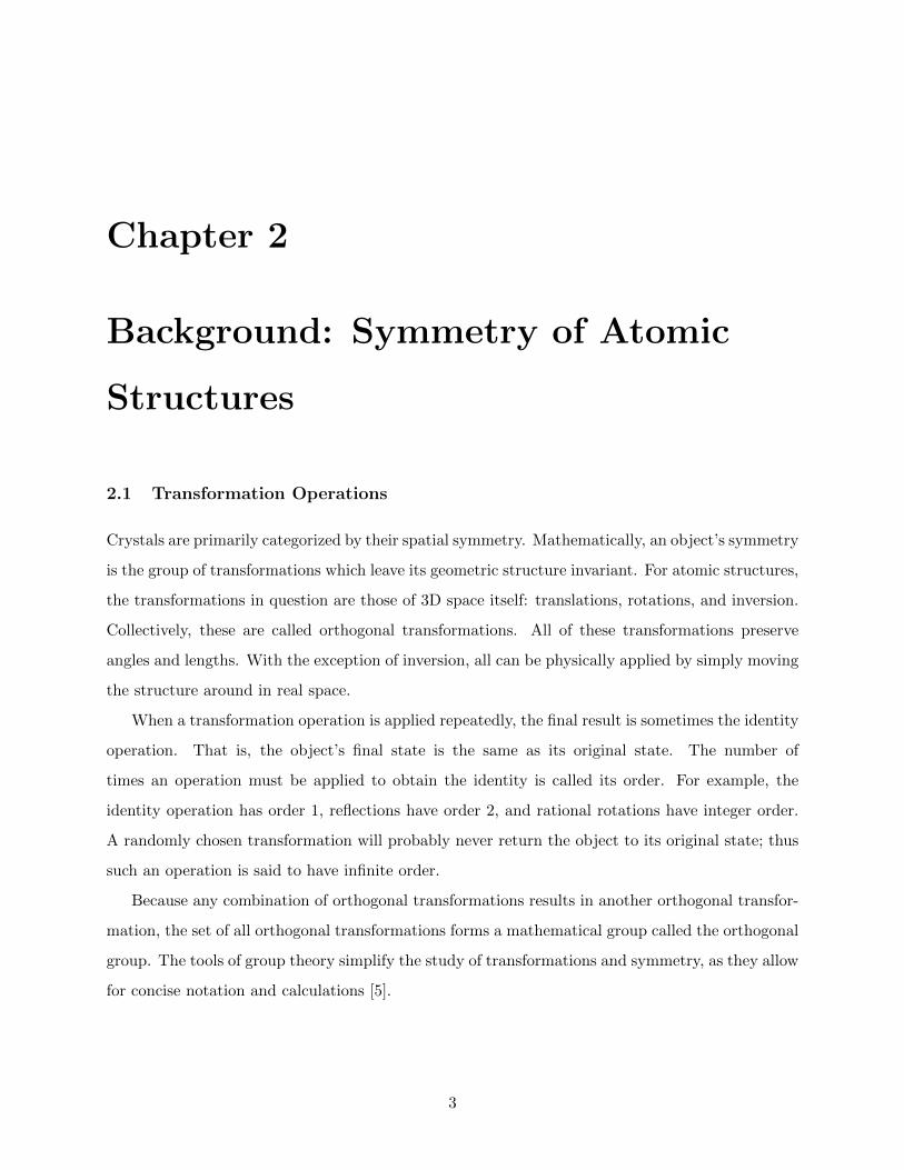
To demonstrate the general utility of pre-symmetrization, random molybdenum clusters were gen-

erated and optimized using the Lennard-Jones potential model [19]. Finding the ground state for

a cluster of given size is an established benchmark for global optimization methods [20]. Here, it

shown that local optimization, combined with PyXtal’s pre-symmetrization, are sufficient to solve

the problem. Clusters were generated of size 38, 55, and 75. For each cluster size, 20,000 structures

were generated: 10,000 with no pre-defined symmetry, and 10,000 with symmetry chosen randomly

from among PyXtal’s 56 built-in point groups. A potential of 4( 1r12− 1

r6) was assigned to each

atom-atom pair. Each structure was locally optimized using SciPy’s optimize.minimize function

[21], using the conjugate gradient (CG) method. As shown in the following figures, the ground state

was found much more frequently when the initial structures possessed some point group symmetry.

With pre-symmetrization, the ground state was found 170 times for size 38 clusters, 254 times for

size 55, and 1 time for size 75. Without pre-symmetrization, the ground state was not found at all.

It is worth noting that while the ground state is found more frequently with pre-symmetrization,

the average energy is higher. This are several possible contributing factors. First, the energy

distribution is generally broader for the pre-symmetrized structures. This suggests that pre-

symmetrization spans the possible structure space more effectively, while asymmetric structures

are more clustered around a specific energy range. Because finding all structures at least once is

more important than finding somewhat low-energy structures multiple times, pre-symmetrization

seems the clear choice for energy optimization.

The probability of finding the ground state is clearly influenced by cluster size, though the

21

exact relationship is unclear from these results. There seem to be at least two competing factors as

the cluster size increases: the increasing expected level of symmetry in the ground state, and the

increasing space of possible structures. In other words, the probability of finding the ground state

naturally goes down with increasing cluster size, but the probability of the ground state having high

symmetry increases. As a result, the net probability would be the highest for intermediate-sized

clusters. More cluster sizes and larger samples would help make any such trends more apparent.

175 150 125 100 75 50 25 0

Energy (eV)

0

200

400

600

800

1000

1200

1400

1600

Counts

LJ cluster: 38 Ground state: -173.9284265117895

no symmetry: 0/10000

random point groups: 170/10000

Figure 4.1: Energy distribution for Lennard Jones size 38 Clusters. The pre-symmetrized struc-tures produce a wider range of energies, reaching nearly all the way up to 0 eV. However, pre-symmetrization also produces more structures at the lowest energies.

4.2 Carbon and Silicon Crystals

A separate test was performed to find the ground states for Carbon and Silicon at 0 K and 0 Pa.

For both elements, 1000 random structures each were generated for 2, 4, 6, 8, and 16 atoms in the

primitive cell. A random space group between 2 and 230 was chosen for each structure. This gave a

total of 5000 structures for each element. Each structure was optimized using VASP [22, 23, 24, 25],

and the final energy was calculated using a single point energy calculation (see appendices B-D for

exact settings). Finally, similar structures were grouped using Pymatgen’s StructureMatcher tool

with a fractional length tolerance of .05, site tolerance of 0.1, and angular tolerance of 5.0 degrees.

22

250 200 150 100 50 0

Energy (eV)

0

500

1000

1500

2000C

ounts

LJ cluster: 55 Ground state: -279.2484703081428

no symmetry: 0/10000

random point groups: 254/10000

Figure 4.2: Energy distribution for Lennard Jones size 55 Clusters. The distribution is similar tothat of size 38, but the ground state is found more frequently. This suggests that symmetry maybecome increasingly important for larger structures.

400 350 300 250 200 150 100 50 0

Energy (eV)

0

500

1000

1500

2000

2500

Counts

LJ cluster: 75 Ground state: -397.4923306811037

no symmetry: 0/10000

random point groups: 1/10000

Figure 4.3: Energy distribution for Lennard Jones size 75 Clusters. The ground state was onlyfound once, making extrapolation difficult. The distribution shape is similar to those of size 38 and55.

23

A total of 2542 unique structures were found for Carbon, and 2306 for Silicon.

(a) (b) (c)

(d) (e) (f)

Figure 4.4: Representative Carbon Structures. These include (a) a graphite-like structure (-9.226eV/atom), (b) diamond (-9.099 eV/atom), (c) lonsdaelite (-9.068 eV/atom), (d) a low-energypentagonal structure also found for silicon (-8.984 eV/atom), (e), a mid-energy structure (-5.888eV/atom), (f) a high-energy structure (-0.009 eV/atom)

For Carbon, the expected structures of diamond and graphite were found, as well as londs-

daelite and various multi-layer graphene structures. The graphene-based structures were not

well-differentiated by energy: there were many slightly different structures varying only by the

displacements between their layers. As a result, these structures were not grouped together by

pymatgen. A prototypical example is shown in figure 4.4. By comparison, most of the remaining

structures appeared to be well-ranked. Structures with higher energies typically had less realistic

bond structures than those with lower energies, and were either too dense or not dense enough.

However, because the lowest energy structures are the most important, a better ranking method

would be useful for further studies. More accurate relaxation methods and energy calculations

would hopefully 1) reduce the number of similar but slightly perturbed structures, and 2) make

the ranking of low-energy structures easier and more accurate. It is clear that systems with weaker

forces between atoms are more sensitive to small changes in energy. This is apparent from the

multi-layer graphene structures, for which the differentiating degrees of freedom involved weak

24

layer-layer forces, and also from the results for water ice (described in the next section).

(a) (b) (c)

(d) (e) (f)

Figure 4.5: Representative Silicon Structures. These include (a) diamond cubic (-5.423 eV/atom),(b) a pentagonal structure (-5.372 eV/atom), (c) another low-energy structure (-5.319 eV/atom),(d) a mid-energy structure with a simple lattice (-4.933 eV/atom), (e) a sparse high-energy structure(-3.488 eV/atom), and (f) a dense high-energy structure (-0.072 eV/atom)

For Silicon, the diamond cubic structure was found many times and had the lowest energy. In

contrast to carbon, there is a rich variety of geometries among the unique lowest-energy structures.

Because most of these structures are based on distorted polygonal rings, it is difficult to tell them

apart without the use of a structure matching tool. However, fewer total unique structures were

found than were for carbon. Additionally, pymatgen was able to more effectively group similar

Silicon structures together. Overall, Silicon appears to have fewer stable structures than Carbon.

Because the allotropes of Silicon are less well-studied than those of Carbon, it is difficult to tell

how accurate the energy rankings are. More accurate calculations would likely be required to do

so.

Figure 4.6b shows the distribution of lattice energies for the final optimized structures. A few

trends are apparent. First, Silicon is more heavily skewed towards the ground state energy than

Carbon. Additionally, the standard deviation for Silicon is smaller. Both of these details suggest

that Silicon has a smaller space of possible low-energy structures. This is expected, since Carbon

25

1 2 3 4 5# of Atoms in Primitive Cell

8

6

4

2

0

Latti

ce E

nerg

y (e

V/at

om)

ab c d

e

fCarbon Crystal Energy Distributions

(a)

1 2 3 4 5# of Atoms in Primitive Cell

5

4

3

2

1

0

Latti

ce E

nerg

y (e

V/at

om)

a bcd

e

fSilicon Crystal Energy Distributions

(b)

Figure 4.6: Lattice Energy Distributions for Carbon and Silicon. The structures from figures 4.4and 4.5 are marked with colored circles. ”+” symbols represent outliers. (±2.7σ). Structures withpositive lattice energies are not included.

26

is known for its ability to form multiple bonds of different types, which in turn should allow it to

form more kinds of stable structures.

Second, the energy landscape appears to be smaller for size-2 primitive cells. It appears that

beyond about 4, the number of atoms in the primitive cell has little influence on the energy distri-

bution. For Carbon and Silicon, the diamond cubic structure has only 2 atoms in its primitive cell.

Thus, it makes sense that increasing the number of atoms would not improve the chances of finding

the ground state. For more complex stoichiometries, it is likely that larger unit cells would produce

better results, since more unique structures would exist for higher-order symmetry groups. Here,

the consistency in energy shows that few new structures are being found for larger primitive cells.

This also suggests that larger Wyckoff positions are not typically stable for single-atom systems.

It is possible that different atomic systems would feature large Wyckoff positions more frequently.

Further study is needed to determine which properties influence the average Wyckoff position size.

27

4.3 3D Ice

A final test was performed for water ice crystals. Random H2O crystals were generated using

PyXtal with between 1 and 4 molecules in the primitive cell. Each structure was then optimized

using a force-field model in LAMMPS (see appendix A for exact settings) [26]. Optimization was

implemented using the materials science Python package ASE [27]. First the FIRE [28] method was

performed, followed by the BFGS [29] method, with a maximum allowed force of 0.001 kcal/(mol-

Angstrom), and a maximum of 1000 steps for each method. If the optimized structure had a stress

value less than 0.001 atm, it was kept. A total of 1000 such optimized structures were generated.

(a) (b) (c)

(d) (e) (f)

Figure 4.7: Representative Ice Structures. (a) cubic ice with a distorted lattice (-14.879 eV/-molecule), (b) A hexaxgonal oxygen structure with different hydrogen bonds (-14.875 eV/molecule),(c) standard ice with distorted oxygen positions (-14.869 eV/molecule), (d) a mid-energy structure(-14.788 eV/molecule), (e) a high-energy layered structure (-14.515 eV/molecule), (f) a differenthigh-energy layered structure (-14.495 eV/molecule)

To avoid redundant calculations, similar structures were grouped together using Pymatgen’s

StructureMatcher tool, again with with a fractional length tolerance of .05, site tolerance of 0.1,

and angular tolerance of 5.0 degrees. This brought the number of unique structures to 275.

It is worth noting that at this point, some the known polymorphs of water ice could already

be recognized. In order to accurately rank the results though, density function theory (DFT)

28

calculations are necessary. This is because force-field models do not take quantum effects or electron

structure into account, and thus the calculated energies are not accurate.

0.07 0.06 0.05 0.04 0.03 0.02 0.01 0.00Force-field Potential Energy (kcal/mol)

14.9

14.8

14.7

14.6

14.5

14.4

14.3

14.2

DFT

Latti

ce E

nerg

y (e

V/m

olec

ule)

Force-Field- vs DFT-optimized Energies of Ice crystals

Figure 4.8: Energy Distribution for H2O Crystals. There is very little correlation between the DFTand Force-field energies. However, there are clear vertical line clusters near -0.01 and -0.02 on thex-axis.

Next, DFT optimization was performed using VASP (see appendices B, C, and D for exact

settings). Two steps of optimization were performed with increasing accuracy, followed by a single

point energy calculation. Some of the original and resulting structures had unrealistic geometries,

such as improper O-H bond structures or unreasonably large or small inter-molecular distances.

Such structures were removed, leaving 227 final structures.

The final structures were ranked based on their single point energy. Six representative structures

are shown in figure 4.7. Standard water ice was found, though it was not the lowest energy structure,

and was very slightly distorted from the expected geometry. Many similar structures were found

which were not considered equivalent by the StructureMatcher tool; as a result, it is difficult to

29

determine exactly how often each structure type appeared. The top-ranking structures which are

sufficiently similar to the shown structures are not included.

It is known that molecular crystal polymorphs are often very close energetically [30]. This

makes ranking difficult, because the difference in energies between structures may be less than the

accuracy of the computation methods. More importantly, multiple polymorphs may be metastable

at a given temperature and pressure. As seen in Figure 4.8, there is no clear trend relating the

force-field and single point energies. This shows that the force-field energy alone is insufficient for

accurate ranking.

However, there are two or three clusters of lines near -0.01 and -0.02 on the x-axes. These lines

are slightly slanted upward to the right. Because the points on these lines are so close together,

it is likely that they belong to the same structural prototypes. If this is the case, then it appears

that small changes in the Force-field energy resulted in relatively large changes in the final DFT

energy for similar structures. This suggests that the DFT calculation did not have sufficient time

or accuracy for complete relaxation. If the relaxation had been sufficient, we would expect similar

structures to relax to approximately the same final energy. This would result in an approximately

horizontal line, which is not seen here. So, it is likely that improving the DFT accuracy would

significantly improve the energy rankings and would make grouping similar structures easier.

30

Chapter 5

Comparison with Existing Tools

Various pieces of software exist to facilitate CSP. Although CSP will typically out-perform experi-

mental trial and error, considerable computation time is still required. Improvements at any level

of the algorithm have the potential to speed up the process by a significant factor. The primary

advantage of PyXtal is its unique method of pre-symmetrization, particularly for molecular and

low-dimensional crystals. This helps reduce the needed number of initial structures, and in turn

the number of calculations to perform.

Furthermore, many existing software packages are either paid or usable on a license-only basis.

To increase accessibility for the materials science community, PyXtal was developed as an open-

source Python package. This way, anyone can use and modify the code as needed, without the

need for access to special computing resources. A few free atomic simulation tools exist, including

LAMMPS and Quantum Espresso, which can be used by anyone. Several other packages are free

for academic users, but require registration or a license key. By combining PyXtal or another

structure generation utility with open source software, it is hypothetically possible for anyone with

a desktop computer to perform CSP for basic systems. PyXtal currently has interface options for

LAMMPS and VASP.

Another potential advantage of PyXtal is its implementation in the Python programming lan-

guage. Python is a popular language among scientists and engineers. A researcher familiar with

Python can easily modify and implement the code for their specific needs. The source code, as well

as detailed documentation, are readily available online. Because structure generation is typically

much faster than simulation, speed is less important than for other steps in the CSP process. Thus,

implementation in a low-level language or library is not as important as it is for most other scientific

applications. With that said, PyXtal makes use of Numpy’s vectorization at several steps in order

31

to optimize the generation speed. For the systems tested, structure generation is significantly faster

than the force-field optimization of the same structure.

Nevertheless, because PyXtal only focuses on the structure generation step of CSP, it is currently

left to the user to determine which kinds of structures to generate. While advancements to machine

learning are helping to automate the process, it is still advisable for a researcher to perform searches

with constraints determined based on prior knowledge and assumptions. For example, if the user

suspects that certain space groups are more likely to occur than others, it would be beneficial

to generate more structures with those space groups. Thus, PyXtal is currently best suited for

someone with both materials science and Python programming experience.

Because PyXtal is only intended as the first step in CSP, it does not perform optimization,

ranking, clustering, or visualization. Users who desire a more complete CSP package and do not

need PyXtal’s features should consider other tools. These include, but are not limited to, USPEX

[2], XtalOpt [31], GRACE [32], and CALYPSO [33].

32

Chapter 6

Limitations and Further Study

6.1 Crystal Structure Prediction Methods Used

For this study, a very basic CSP method was used. Random structures were generated and then

optimized in an essentially trial-and-error way. The only significant improvements were PyXtal’s

pre-symmetrization scheme and the grouping of similar structures using Pymatgen. More advanced

CSP techniques can drastically reduce the time needed to find the ground state. Such techniques

might include genetic algorithms and mutations, better ranking systems, machine learning, or dif-

ferent optimization methods. Of course, the implementation of more advanced techniques comes

with its own challenges, namely a proper software implementation and more complex background

knowledge. Some of the tools mentioned in the previous section implement such techniques. How-

ever, the primary goal of this thesis is to demonstrate that PyXtal can be used for CSP in general.

Because PyXtal can be called using customized Python scripts, other pieces of software could hy-

pothetically implement it within more advanced CSP algorithms. It is the author’s hope that the

original features found in PyXtal will be utilized by other researchers in this way.

6.2 Complexity of the Systems Studied

The crystal systems studied in this thesis are relatively simple. A more rigorous test of PyXtal’s

abilities would involve finding the ground state for an unknown or very complex system. Increased

complexity could involve a larger number of atoms in the unit cell, metallic atoms with more

complicated valence mechanics, or more than one kind of atomic specie. The introduction of more

species may necessitate a larger space of possible structures, since the stoichiometry of the ground

state may not be known. For example, to determine the convex hull for a poly-atomic system,

33

one would need to generate structures having different ratios of each atomic specie. While PyXtal

is capable of generating such structures, it is up to the user to define each possible stoichiometry

separately.

6.3 Molecular Flexibility

An inherent limitation of PyXtal is that molecules are assumed to be rigid; no stereoisomers of

any kind are considered. For H2O this is not an issue, because the molecule is simple enough that

most perturbations will not alter the bond structure. But for larger molecules, especially those

with many degrees of freedom, this approach may be insufficient. The ground state crystal could

potentially have different molecular configuration or bond angles than those supplied.

The problem of pre-symmetrization becomes much more complicated when molecules are given

flexibility. It is then necessary to determine whether a given perturbation will change the symmetry

or not, and the resulting symmetry group must be calculated. It may be theoretically possible to

analyze the symmetry of every relevant molecular geometry. However, the space of all possible

configurations may be highly complex and nontrivial, which in turn would lead to more structures

needing to be generated.

A partial solution would be to input multiple configurations of the molecule before generation.

If the molecular configuration space is sufficiently sampled, then the molecules may be able to relax

into the correct geometry during optimization. Of course, as the molecular complexity grows, the

number of configuration samples would also need to grow. If more than a few degrees of freedom

are present, the number could quickly grow beyond computational limits. Efficient handling of

complex molecular systems remains a computationally challenging problem.

6.4 Non-crystalline Systems

Another inherent limitation of PyXtal is that it only handles classical crystal structures. This

means that amorphous structures, quasi-crystals, order-disorder systems, and host-guest systems

cannot be directly generated. The study of these kinds of systems would require a generalization

of the mathematics used by PyXtal. For example, the treatment of quasi-crystals involves the use

of hyper-dimensional symmetry groups [34], whereas PyXtal only allows for groups of 3 or fewer

dimensions. It is hypothetically possible that such systems could be found during the optimization

stage, provided a large enough supercell is used. But in this case, one might as well forgo symmetry

34

and generate completely random initial structures. PyXtal is best used when the ground state is

suspected to possess standard crystal symmetry.

35

Chapter 7

Conclusion

This thesis has covered the conceptual background for the original software package PyXtal. The

core features of PyXtal have been highlighted, with further documentation available online. The

primary new feature - special Wyckoff positions for molecular crystals - has been described in detail,

and its usefulness has been demonstrated by quickly finding the ground state of water ice.

PyXtal, along with its source code and documentation, is currently available online at https:

//github.com/qzhu2017/PyXtal. Further development will continue as different needs arise.

Examples for 0D atomic, 3D atomic, and 3D molecular structures have been provided. For

each case, the ground state was found within a few thousand generation attempts. This shows that

PyXtal is sufficient for generating random crystal structures.

While several improvements could be made to PyXtal, its original goals have been achieved. It

has been shown that proper handling of symmetry is useful for efficiently and accurately searching

the energy landscape. Furthermore, the utility of symmetry groups and Wyckoff positions as

a basis for hypothetical structures suggests the possibility of more fundamental representations.

Further development and application of the mathematical background should enable more complex

structure types to be studied in the future.

36

Appendix A

LAMMPS Settings Used for H2O

clear

units electron

boundary p p p

atom_modify sort 0 0.0

### interactions

atom_style full

pair_style lj/cut/tip4p/long 1 2 1 1 0.278072379 17.007

bond_style class2

angle_style harmonic

kspace_style pppm/tip4p 0.0001

read_data tmp/data.lammps

pair_coeff 2 2 0 0

pair_coeff 1 2 0 0

pair_coeff 1 1 0.000295147 5.96946

neighbor 2.0 bin

min_style cg

minimize 1e-6 1e-6 10000 10000

thermo_style custom pe pxx

thermo_modify flush yes

thermo 1

run 0

37

Appendix B

VASP INCAR for DFT Optimization

Step 1

INCAR created by Atomic Simulation Environment

KSPACING = 0.400000

POTIM = 0.020000

PSTRESS = 0.000000

EDIFF = 1.00e-02

ALGO = normal

GGA = PE

PREC = low

IBRION = 2

ISIF = 4

NPAR = 8

NSW = 10

KGAMMA = .TRUE.

LCHARG = .FALSE.

LWAVE = .FALSE.

38

Appendix C

VASP INCAR for DFT Optimization

Step 2

INCAR created by Atomic Simulation Environment

KSPACING = 0.300000

POTIM = 0.050000

PSTRESS = 0.000000

EDIFF = 1.00e-03

ALGO = normal

GGA = PE

PREC = normal

IBRION = 2

ISIF = 3

NPAR = 8

NSW = 25

KGAMMA = .TRUE.

LCHARG = .FALSE.

LWAVE = .FALSE.

39

Appendix D

VASP INCAR for DFT Single Point

Energy Calculations

INCAR created by Atomic Simulation Environment

ENCUT = 600.000000

KSPACING = 0.150000

PSTRESS = 0.000000

EDIFF = 1.00e-04

GGA = PE

PREC = accurate

IBRION = 2

ISIF = 3

NPAR = 8

NSW = 0

KGAMMA = .TRUE.

LCHARG = .FALSE.

LWAVE = .FALSE.

40

Bibliography

[1] K. D. M. Harris and M. Tremayne, “Crystal structure determination from powder diffraction

data,” Chemistry of Materials, vol. 8, no. 11, pp. 2554–2570, 1996. [Online]. Available:

https://doi.org/10.1021/cm960218d

[2] A. Oganov, Y. ma, C. Glass, and M. Valle, “Evolutionary crystal structure prediction:

Overview of the uspex method and some of its applications,” Psi-k Newsl., vol. 84, 01 2007.

[3] P. Avery and E. Zurek, “Randspg: An open-source program for generating atomistic crystal

structures with specific spacegroups,” Computer Physics Communications, vol. 213, pp. 208–

216, 2017.

[4] Q. Zhu, A. Oganov, C. Glass, and H. T Stokes, “Constrained evolutionary algorithm for struc-

ture prediction of molecular crystals: Methodology and applications,” Acta crystallographica.

Section B, Structural science, vol. 68, pp. 215–26, 06 2012.

[5] B. Souvignier, “Chapter 1.1. a general introduction to groups,” International Tables for Crys-

tallography, vol. A, pp. 2–11, 2016.

[6] H. Wondratschek and M. I. Aroyo, “Chapter 1.2. crystallographic symmetry,” International

Tables for Crystallography, vol. A, pp. 12–21, 2016.

[7] M. I. A. H. D. F. K. M. Th. Hahn, A. Looijenga-Vos and P. Konstantinov, “2.1. guide to the

use of the space-group tables,” International Tables for Crystallography, vol. A, pp. 142–144,

2016.

[8] A. Vince, “Periodicity, quasiperiodicity, and bieberbach’s theorem on crystallographic

groups,” The American Mathematical Monthly, vol. 104, no. 1, pp. 27–35, 1997. [Online].

Available: http://www.jstor.org/stable/2974820

[9] D. Shechtman, I. Blech, D. Gratias, and J. W. Cahn, “Metallic phase with long-range

orientational order and no translational symmetry,” Phys. Rev. Lett., vol. 53, pp. 1951–1953,

Nov 1984. [Online]. Available: https://link.aps.org/doi/10.1103/PhysRevLett.53.1951

[10] A. Yamamoto, “Software package for structure analysis of quasicrystals. sci technol adv

mater. 2008 mar 6;9(1):013001. doi,” in PubMed PMID: 27877919; PubMed Central PMCID:

PMC5099788, pp. 10–1088.

[11] M. I. A. G. C. B. Souvignier, H. Wondratschek and A. M. Glazer, “Chapter 1.4. space groups

and their descriptions,” International Tables for Crystallography, vol. A, pp. 42–74, 2016.

41

[12] S. R. Hall, F. H. Allen, and I. D. Brown, “The crystallographic information file (CIF): a new

standard archive file for crystallography,” Acta Crystallographica Section A, vol. 47, no. 6,

pp. 655–685, Nov 1991. [Online]. Available: https://doi.org/10.1107/S010876739101067X

[13] (2019, Feb) Poscar. University of Vienna CMS. [Online]. Available: https://cms.mpi.univie.

ac.at/wiki/index.php/POSCAR

[14] B. S. H. Wondratschek, M. I. Aroyo and G. Chapuis, “Chapter 1.5. transformations of coor-

dinate systems,” International Tables for Crystallography, vol. A, pp. 75–105, 2015.

[15] S. P. Ong, W. D. Richards, A. Jain, G. Hautier, M. Kocher, S. Cholia, D. Gunter, V. L.

Chevrier, K. A. Persson, and G. Ceder, “Python materials genomics (pymatgen): A robust,

open-source python library for materials analysis,” Computational Materials Science, vol. 68,

pp. 314 – 319, 2013. [Online]. Available: http://www.sciencedirect.com/science/article/pii/

S0927025612006295

[16] L. Babai, “On lovasz’ lattice reduction and the nearest lattice point problem,” Combinatorica,

vol. 6, no. 1, pp. 1–13, Mar 1986. [Online]. Available: https://doi.org/10.1007/BF02579403

[17] U. M. ller, “3.2.4. molecular symmetry,” International Tables for Crystallography, vol. A, p.

72776, 2016.

[18] I.-H. Suh, K. H. Park, W. P. Jensen, and D. E. Lewis, “Molecules, crystals, and

chirality,” Journal of Chemical Education, vol. 74, no. 7, p. 800, 1997. [Online]. Available:

https://doi.org/10.1021/ed074p800

[19] J. E. Jones and S. Chapman, “On the determination of molecular fields.—i. from

the variation of the viscosity of a gas with temperature,” Proceedings of the Royal Society

of London. Series A, Containing Papers of a Mathematical and Physical Character, vol. 106,

no. 738, pp. 441–462, 1924. [Online]. Available: https://royalsocietypublishing.org/doi/abs/

10.1098/rspa.1924.0081

[20] D. J. Wales and J. P. K. Doye, “Global optimization by basin-hopping and the lowest

energy structures of lennard-jones clusters containing up to 110 atoms,” The Journal

of Physical Chemistry A, vol. 101, no. 28, pp. 5111–5116, 1997. [Online]. Available:

https://doi.org/10.1021/jp970984n

[21] E. Jones, T. Oliphant, P. Peterson et al., “SciPy: Open source scientific tools for Python,”

2001–, [Online; accessed ¡today¿]. [Online]. Available: http://www.scipy.org/

[22] G. Kresse and J. Hafner, “Ab initio molecular dynamics for liquid metals,” Phys. Rev.

B, vol. 47, pp. 558–561, Jan 1993. [Online]. Available: https://link.aps.org/doi/10.1103/

PhysRevB.47.558

[23] ——, “Ab initio molecular-dynamics simulation of the liquid-metal–amorphous-semiconductor

transition in germanium,” Phys. Rev. B, vol. 49, pp. 14 251–14 269, May 1994. [Online].

Available: https://link.aps.org/doi/10.1103/PhysRevB.49.14251

42

[24] G. Kresse and J. Furthmller, “Efficiency of ab-initio total energy calculations for metals and

semiconductors using a plane-wave basis set,” Computational Materials Science, vol. 6, pp.

15–50, 07 1996.

[25] G. Kresse and J. Furthmuller, “Efficient iterative schemes for ab initio total-energy

calculations using a plane-wave basis set,” Phys. Rev. B, vol. 54, pp. 11 169–11 186, Oct 1996.

[Online]. Available: https://link.aps.org/doi/10.1103/PhysRevB.54.11169

[26] S. Plimpton, “Fast parallel algorithms for short-range molecular dynamics,” Journal

of Computational Physics, vol. 117, no. 1, pp. 1 – 19, 1995. [Online]. Available:

http://www.sciencedirect.com/science/article/pii/S002199918571039X

[27] A. H. Larsen, J. J. Mortensen, J. Blomqvist, I. E. Castelli, R. Christensen, M. Du lak,

J. Friis, M. N. Groves, B. Hammer, C. Hargus, E. D. Hermes, P. C. Jennings, P. B.

Jensen, J. Kermode, J. R. Kitchin, E. L. Kolsbjerg, J. Kubal, K. Kaasbjerg, S. Lysgaard,

J. B. Maronsson, T. Maxson, T. Olsen, L. Pastewka, A. Peterson, C. Rostgaard, J. Schiøtz,

O. Schtt, M. Strange, K. S. Thygesen, T. Vegge, L. Vilhelmsen, M. Walter, Z. Zeng, and

K. W. Jacobsen, “The atomic simulation environment—a python library for working with

atoms,” Journal of Physics: Condensed Matter, vol. 29, no. 27, p. 273002, jun 2017. [Online].

Available: https://doi.org/10.1088%2F1361-648x%2Faa680e

[28] E. Bitzek, P. Koskinen, F. Gahler, M. Moseler, and P. Gumbsch, “Structural relaxation

made simple,” Phys. Rev. Lett., vol. 97, p. 170201, Oct 2006. [Online]. Available:

https://link.aps.org/doi/10.1103/PhysRevLett.97.170201

[29] J. D. Head and M. C. Zerner, “A broydenfletchergoldfarbshanno optimization procedure

for molecular geometries,” Chemical Physics Letters, vol. 122, no. 3, pp. 264 – 270, 1985.

[Online]. Available: http://www.sciencedirect.com/science/article/pii/0009261485805741

[30] S. A.-E. G. B. J. B. S. G. G. H. Y. H. R. H. Y. H. A. K. K. N. A. O. C. P. B. R. R.

S. W. T. S. W. C. W. X.-F. Z. Q. Z. C.S. Adjiman, A. Aspuru-Guzik, Topics in Cur-

rent Chemistry 345: Prediction and Calculation of Crystal Structures ule Atahan-EvrenkAln

Aspuru-GuzikEditorsMethods and Applications, ule Atahan-Evrenk and A. Aspuru-Guzik, Eds.

Springer, 2014.

[31] D. C. Lonie and E. Zurek, “Xtalopt: An open-source evolutionary algorithm for crystal

structure prediction,” Computer Physics Communications, vol. 182, no. 2, pp. 372 – 387, 2011.

[Online]. Available: http://www.sciencedirect.com/science/article/pii/S0010465510003140

[32] J. Hoja, H.-Y. Ko, M. A. Neumann, R. Car, R. A. DiStasio, and A. Tkatchenko, “Reliable and

practical computational description of molecular crystal polymorphs,” Science Advances, vol. 5,

no. 1, 2019. [Online]. Available: https://advances.sciencemag.org/content/5/1/eaau3338

[33] Y. Wang, J. Lv, L. Zhu, and Y. Ma, “Calypso: A method for crystal structure prediction,”

Computer Physics Communications, vol. 183, no. 10, pp. 2063 – 2070, 2012. [Online].

Available: http://www.sciencedirect.com/science/article/pii/S0010465512001762

43

[34] P. M. de Wolff, T. Janssen, and A. Janner, “The superspace groups for incommensurate crystal

structures with a one-dimensional modulation,” Acta Crystallographica Section A, vol. 37,

no. 5, pp. 625–636, Sep 1981. [Online]. Available: https://doi.org/10.1107/S0567739481001447

44

Curriculum Vitae

Graduate College

University of Nevada, Las Vegas

Scott Fredericks

scottwfredericks@gmail.com

Degrees:

Bachelor of Science in Physics 2011

University of Arkansas, Fayetteville, AR

Thesis Examination Committee:

Chairperson, Qiang Zhu, Ph.D.

Committee Member, Dr. Ashkan Salamat, Ph.D.

Committee Member, Dr. Tao Pang, Ph.D.

Graduate Faculty Representative, Dr. Hui Zhao, Ph.D.

45