Applied Soft Com puting Multi-objective optimization of ...
14
Applied Soft Computing 28 (2015) 30ȸ43 Multi-objective optimization of the stack of a thermoacoustic engine using GAMS L.K. Tartibu a,∗ , B. Sun b , M.A.E. Kaunda b a Department of Mechanical Engineering, Mangosuthu University of Technology, Box 12363, Durban 4026, South Africa b Department of Mechanical Engineering, Cape Peninsula University of Technology, Box 652, Cape Town 8000, South Africa a r t i c l e i n f o a b s t r a c t Article history: Received 8 May 2013 Received in revised form 21 October 2014 Accepted 30 November 2014 Available online 9 December 2014 Keywords: Thermoacoustics engine Multi-objective optimization GAMS Mathematical programming This work illustrates the use of a multi-objective optimization approach to model and optimize the performance of a simple thermoacoustic engine. System parameters and constraints that capture the underlying thermoacoustic dynamics have been used to define the model. Work output, viscous loss, conductive heat loss, convective heat loss and radiative heat loss have been used to measure the per- formance of the engine. The optimization task is formulated as a five-criterion mixed-integer non-linear programming problem. Since we optimize multiple objectives simultaneously, each objective component has been given a weighting factor to provide appropriate user-defined emphasis. A practical example is given to illustrate the approach. We have determined a design statement of a stack describing how the design would change if emphasis is given to one objective in particular. We also considered optimiza- tion of multiple objectives components simultaneously and identify global optimal solutions describing the stack geometry using the augmented ε-constraint method. This approach has been implemented in GAMS (General Algebraic Modelling System). 1. Introduction This work demonstrates how multi-objective optimization techniques can be used to optimize the design and performance of small-scale thermoacoustic devices. Thermoacoustics relates to the physical phenomenon that a temperature difference can cre- ate and amplify a sound wave and vice versa [1]. Hereto the sound wave is brought into interaction with a porous solid material with a much higher heat capacity compared to the gas through which the sound wave propagates. The solid material acts as a regenerator. When a temperature difference is applied across this stack and a sound wave passes through the stack from the cold to the hot side, a parcel of gas executes a thermoacoustic cycle. The gas will subse- quently be compressed, displaced and heated, expanded, displaced again and cooled (Fig. 1). During this cycle the gas is being com- pressed at low temperature, while expansion takes place at high temperature. This means that work is performed on the gas. The effect of this work is that the pressure amplitude of the sound wave is increased. In this way it is possible to create and amplify a sound wave by a temperature difference. The thermal energy is converted into acoustic energy. Within thermoacoustics, this is referred to as a thermoacoustic engine (TAE). In a thermoa- coustic refrigerator (TAR), the thermodynamic cycle is run in the reverse way and heat is pumped from a low-temperature level to a high-temperature level by the acoustic power. The basic mechan- ics behind thermoacoustics are already well understood. A detailed explanation of the way thermoacoustic coolers work is given by Swift [1] and Wheatley et al. [2]. Recent researches focuses on optimizing the modelling approach so that thermoacoustic coolers can compete with commercial refrigerators. After reviewing some fundamental physical properties and previous optimization effort underlying thermoacoustic devices, we will then proceed to discuss our approach to optimize their design. 1.1. Thermoacoustic engines The most important part of the thermoacoustic system is the core, where the stack of plates is. Thermoacoustic effects actu- ally occur within a very small layer next to the plate, the thermal boundary layer. It is defined as [3]: I 2K ı k = (1) pmcpω ∗ Corresponding author. Tel.: +27783104904; fax: +27866401810. E-mail address: [email protected] (L.K. Tartibu). with K being the thermal conductivity, pm the mean density, cp the constant pressure specific heat of the working fluid. Heat transfer http://dx.doi.org/10.1016/j.asoc.2014.11.055 1568-4946 Applied Soft Computing
Transcript of Applied Soft Com puting Multi-objective optimization of ...
Applied Soft Computing 28 (2015) 30 43
Multi-objective optimization of the stack of a thermoacoustic engine using GAMS
L.K. Tartibu a,∗ , B. Sunb, M.A.E. Kaunda b
a Department of Mechanical Engineering, Mangosuthu University of Technology, Box 12363, Durban 4026, South Africa
b Department of Mechanical Engineering, Cape Peninsula University of Technology, Box 652, Cape Town 8000, South Africa
a r t i c l e i n f o a b s t r a c t
Article history:
Received 8 May 2013
Received in revised form 21 October 2014
Accepted 30 November 2014
Available online 9 December 2014
Keywords:
Thermoacoustics engine
Multi-objective optimization
GAMS
Mathematical programming
This work illustrates the use of a multi-objective optimization approach to model and optimize the
performance of a simple thermoacoustic engine. System parameters and constraints that capture the
underlying thermoacoustic dynamics have been used to define the model. Work output, viscous loss,
conductive heat loss, convective heat loss and radiative heat loss have been used to measure the per-
formance of the engine. The optimization task is formulated as a five-criterion mixed-integer non-linear
programming problem. Since we optimize multiple objectives simultaneously, each objective component
has been given a weighting factor to provide appropriate user-defined emphasis. A practical example is
given to illustrate the approach. We have determined a design statement of a stack describing how the
design would change if emphasis is given to one objective in particular. We also considered optimiza-
tion of multiple objectives components simultaneously and identify global optimal solutions describing
the stack geometry using the augmented ε-constraint method. This approach has been implemented in
GAMS (General Algebraic Modelling System).
1. Introduction
This work demonstrates how multi-objective optimization
techniques can be used to optimize the design and performance
of small-scale thermoacoustic devices. Thermoacoustics relates to
the physical phenomenon that a temperature difference can cre-
ate and amplify a sound wave and vice versa [1]. Hereto the sound
wave is brought into interaction with a porous solid material with a
much higher heat capacity compared to the gas through which the
sound wave propagates. The solid material acts as a regenerator.
When a temperature difference is applied across this stack and a
sound wave passes through the stack from the cold to the hot side,
a parcel of gas executes a thermoacoustic cycle. The gas will subse-
quently be compressed, displaced and heated, expanded, displaced
again and cooled (Fig. 1). During this cycle the gas is being com-
pressed at low temperature, while expansion takes place at high
temperature. This means that work is performed on the gas.
The effect of this work is that the pressure amplitude of the
sound wave is increased. In this way it is possible to create and
amplify a sound wave by a temperature difference. The thermal
energy is converted into acoustic energy. Within thermoacoustics,
this is referred to as a thermoacoustic engine (TAE). In a thermoa-
coustic refrigerator (TAR), the thermodynamic cycle is run in the
reverse way and heat is pumped from a low-temperature level to a
high-temperature level by the acoustic power. The basic mechan-
ics behind thermoacoustics are already well understood. A detailed
explanation of the way thermoacoustic coolers work is given by
Swift [1] and Wheatley et al. [2]. Recent researches focuses on
optimizing the modelling approach so that thermoacoustic coolers
can compete with commercial refrigerators. After reviewing some
fundamental physical properties and previous optimization effort
underlying thermoacoustic devices, we will then proceed to discuss
our approach to optimize their design.
1.1. Thermoacoustic engines
The most important part of the thermoacoustic system is the
core, where the stack of plates is. Thermoacoustic effects actu-
ally occur within a very small layer next to the plate, the thermal
boundary layer. It is defined as [3]: I
2K
ık = (1) pmcpω
∗ Corresponding author. Tel.: +27783104904; fax: +27866401810.
E-mail address: [email protected] (L.K. Tartibu).
with K being the thermal conductivity, pm the mean density, cp the
constant pressure specific heat of the working fluid. Heat transfer
http://dx.doi.org/10.1016/j.asoc.2014.11.055
1568-4946
Applied Soft Computing


L.K. Tartibu et al. / Applied Soft Computing 28 (2015) 30–43 31
1
Fig. 1. Typical fluid parcels, near a stack plate, executing the four steps (1 4) of the
thermodynamic cycle in a stack-based standing-wave thermoacoustic engine.
by conduction is encouraged by a thick boundary layer during a
period of 1/ω, where ω is the angular frequency of the vibrating
fluid. However, another layer that occurs next to the plate, the vis-
cous boundary layer, discourages the thermoacoustic effects. It is
defined as [3]: I
2µ
programme developed with DELTAE shows that the efficiency of
thermoacoustic coolers is sensitive to stack length, position, mean
pressure and gas mixture (Prandtl number), and less sensitive to the
stack spacing. A systematic design optimization of thermoacoustic
coolers is proposed by Wetzel and Herman [10]. A model based
on the boundary layer approximation and the short stack assump-
tion has been developed to calculate the work flux and heat flux.
Nineteen design variables are optimized to achieve the best COP.
The influence of the plate spacing in the stack on the behaviour of
the refrigerator was investigated systematically by Tijani et al. [3].
Optimal plate spacing was identified for thermoacoustic refrigera-
tion. The effect of drive ratio, plate thickness, heat exchanger length
and position on the performance of thermoacoustic refrigerator and
the flow behaviour is analyzed by Besnoin [11]. The results indicate
cooling load peak at a well-defined combination of heat exchanger
thickness, length, and width of the gap between the heat exchanger ıV = (2)
pmω and the stack plates. The optimization of an inertance segment used
where µ is the diffusivity of the gas. Losses due to viscous effects
occur in this region. A thinner viscous boundary layer than the
thermal boundary layer is desirable for effective thermoacoustic
effects. Swift [1] started with the equation of heat transfer to come
up with a theoretical critical mean temperature gradient, ▽Tcrit. that
describes the difference between a thermoacoustic heat engine and
a refrigerator,
ωps
in a standing-wave type heat-driven thermoacoustic device is con-
sidered by Zoontjens et al. [12]. This study suggests that the vast
array of variables which affect the system performance must all be
considered as interdependent for robust device operation. This is by
no means a complete list of the optimization of engine components,
but it is a good overview of optimization targets.
A common trait of all these studies is the utilization of a linear
approach while trying to optimize the device. Additionally, most
studies (the exception being the Minner et al. s [9] study) have been Tcrit. = 1
pmcpus
(3) limited to parametric studies to estimate the effect of single design
parameters on device performance and ignored thermal losses to This critical temperature gradient depends on the angular fre-
quency ω, the first order pressure ps and velocity us in the standing the surroundings. These parametric studies are unable to capture
1 1 the nonlinear interactions inherent in thermoacoustic models with wave, as well as the mean gas density pm and specific heat cp.
In a TAE, the imposed temperature gradient must be greater than
this critical temperature gradient I' = (dT/dx)/(dT/dxcrit.) > 1, while
in TARs the critical temperature gradient upper bounds its per-
formance (dT/dx)/(dT/dxcrit.) < 1 [4]. Fig. 2 shows a very simple
prototypical standing wave TAE.
The closed end of the resonance tube is the velocity node and
the pressure antinode. The porous stack is located near the closed
end and the interior gas experiences large pressure oscillations and
relatively small displacement. Heat input is provided by a heating
wire, causing a temperature gradient to be established across the
stack (in the axial direction). A gas in the vicinity of the walls inside
the regenerative unit experiences compression, expansion and dis-
placement when it is subject to a sound wave. Over the course of
the cycle, heat is added to the gas at high pressure, and heat is with-
drawn from it at low pressure. This energy imbalance results in an
increase of the pressure amplitude from one cycle to the next, until
the acoustic dissipation of the sound energy equals the addition of
heat to the system [4 8].
1.2. Optimization in thermoacoustics
Various parameters affecting the performance of thermoa-
coustic devices are well understood from previous studies. The
optimization of a thermoacoustic system is considered by Min-
ner et al. [9] through a parametric study. The design optimization
Fig. 2. Prototype of a small-scale thermoacoustic engine or prime mover.
multiple variables, and could only guarantee locally optimal solu-
tions. Ueda et al. [13] consider varying the position, length, and flow
channel radius of the regenerator of a travelling wave thermoacous-
tic refrigerator and optimize them simultaneously. The obtained
results show an increase of the Carnot COP by 60%. Zink et al.
[14] illustrate the optimization of thermoacoustic systems, while
taking into account thermal losses to the surroundings that are typ-
ically disregarded. They have targeted a thermoacoustic engine as a
starting point. A model has been built in order to develop an under-
standing of the importance of the trade-offs between the acoustic
and thermal parameters. They use mathematical analysis and opti-
mization, a design aid that is under-utilized in thermoacoustic
community. The optimization considers four weighted objectives
(these are the conductive heat flux from the stack s outer surface,
the conduction through the stack, acoustic work and viscous resis-
tance) and is conducted with the Nelder Mead Simplex method. A
recent study by Trapp et al. [15] presented analytical solutions for
cases of single objective optimization that identify globally optimal
parameter levels. Optimization of multiple objective components
(acoustic work, viscous resistance and heat fluxes) has been consid-
ered, efficient frontier of Pareto optimal solutions corresponding to
selected weights have been generated and two profiles have been
constructed to illustrate the conflicting nature of those objective
component. Zink et al. [14] and Trapp et al. [15] studies show that
geometrical parameters describing the stack are interdependent.
1.3. Motivations
Linear approximation used for the design modelling of thermoa-
coustic systems functions very well. A numerical model that couple
one dimensional linear acoustics in the resonator with a low Mach
number viscous and conducting flow in the stack/heat exchang-
ers section was developed by Hireche et al. [16]. The results show
that the model successfully captures the dynamics of the static
process and allow exploring the engine efficiency. Interestingly, a
study conducted at the Energy Research Centre of the Netherlands

32 L.K. Tartibu et al. / Applied Soft Computing 28 (2015) 30–43
Fig. 3. Heat flow from the power supply partitioned by the losses from radiation,
conduction, convection and the power input.
Adapted from [18].
[17] shows that the ratio between thermal losses and acoustic
power changes with increasing acoustic power for thermoacous-
tic devices. It suggests that heat losses by convection, conduction
and radiation need to be adequately covered in the modelling espe-
cially with regards to miniaturization of the devices where thermal
losses are expected to increase [14].
McLaughlin [18] has thoroughly analyzed the heat transfer for
a Helmholtz-like resonator, 1.91 cm in diameter and 3.28 cm in
length. The loss to conduction has been estimated as 40% of the
input power. The losses from convection inside and outside of the
device have been estimated as 38%. Radiation accounts for 10% of
the input power. This leaves only 12% of input power that can be
used to produce acoustic work (Fig. 3). Although these losses are
approximations not meant to be highly accurate determinations,
they suggest that these losses are significant when compared to
total heat input and should be considered as design criterion. There-
fore, this work aims to highlight one methodology to incorporate
thermal losses in the design process.
In spite of the introductory nature of Zink et al. [14] and Trapp
et al. [15] studies with respect of their plans to expand it and
include a driven thermoacoustic refrigerators, the presented works
are important contributions to thermoacoustics as it merges the
theoretical optimization approach with thermal investigation in
thermoacoustics. However, through the objective function weights,
a significant amount of personal preference is available to place
desired emphasis. The scaling of the objective functions has strong
influence in the obtained results. Therefore since several conflicting
objectives have been identified, an effort to effectively imple-
ment the augmented ε-constraint method for producing the Pareto
optimal solutions in a multi-objective optimization mathemati-
cal programming method is carried out in our approach. This has
been implemented in the modelling language GAMS [19] (General
Algebraic Modelling Language, www.gams.com). As a result, GAMS
codes are written to define, to analyze, and solve optimization prob-
lems to generate sets of Pareto optimal solutions unlike previous
studies.
• optimizing its geometrical parameters namely the stack length,
the stack height, the stack position, the number of channels and
the plate spacing.
Specific sub-objective is as follows:
• providing guidance to the decision maker on the choice of optimal
geometry of thermoacoustic devices.
The remainder of this paper is organized in the following
fashion: in Section 2, the modelling approach is presented. The
fundamental components of our mathematical model character-
izing the standing wave thermoacoustic heat engine are presented
in Section 3. In Section 4, we discuss single objective optimization,
using weighted sum method to find values of the variables that
satisfy the constraints and are globally optimal with respect to the
considered objective function. Section 5 considers multi-objective
optimization using epsilon constraint method. Section 6 reports the
contribution of this work.
2. Modelling approach
In this section, our modelling approach for the physical stand-
ing wave engine depicted in Fig. 2 is discussed; the development
of our mathematical model and its corresponding optimization is
included in Sections 3 and 4. The problem is reduced to a two
dimensional domain, because of the symmetry present in the stack.
Two constant temperature boundaries are considered namely one
convective boundary and one adiabatic boundary, as shown in
Fig. 4. For our model, only the stack geometry is considered; the
model considers variation in operating condition and the interde-
pendence of stack location and geometry.
Five different parameters are considered to characterize the
stack:
• L: stack length,
• H: stack height,
• Za: stack placement (with Za = 0 corresponding to the closed end
of the resonator tube), • dc: channel diameter, and
• N: number of channels.
Those parameters have been allowed to vary simultaneously.
Five different objectives as described by Trapp et al. [15] namely
two acoustic objectives (acoustic work W of the thermoacous-
tic engine and viscous resistance RV through the stack [1,20] and
three thermal objectives (convective heat flow Qconv, radiative
heat flow Qrad, and conductive heat flow Qcond) are considered
to measure the quality of a given set of variable value that sat-
isfies all of the constraints. Because work is the only objective
to be maximized, we instead minimize its negative magnitude
along with all of the other components. Ultimately, optimizing
the resulting problem generates optimal objective function value G∗ = [W ∗, R∗ , Q ∗ , Q ∗ , Q ∗ ] and optimal solution x∗ = [L∗, H∗,
V conv rad cond
1.4. Research goals
The purpose of the stack is to provide a medium where the walls
are close enough so that each time a parcel of gas moves, the tem-
perature differential is transferred to the wall of the stack. Their
geometry and position are crucial for the performance of the device.
The primary objectives of the present research are as follows:
• developing a new optimization scheme combining acoustic work,
viscous resistance and thermal losses as objective functions in
small-scale thermoacoustic engine design and
dc∗, Za∗, N∗]. Since the five objectives are conflicting in nature
[15,21], a multi-objective optimization approach has been used.
Since we optimize multiple objective components simultaneously,
each objective component has been given a weighting factor wi to
provide appropriate user-defined emphasis.
According to Hwang and Masud [22], the methods for solv-
ing multi-objective mathematical programming problems can be
classified into three categories, based on the phase in which
the decision maker is involved in the decision making process
expressing his/her preferences: the a priori methods, the interac-
tive methods and the a posteriori or generation methods. The a

L.K. Tartibu et al. / Applied Soft Computing 28 (2015) 30–43 33
1
C
Fig. 4. Computational domain.
posteriori (or generation) methods give the whole picture (i.e.
the Pareto set) to the decision maker, before his/her final choice,
reinforcing thus, his/her confidence to the final decision. In gen-
eral, the most widely used generation methods are the weighting
(4) Free convection and radiation to surroundings (at T∞) with tem-
perature dependent heat transfer coefficient (h), emissivity ε, and thermal conductivity (k):
method and the ε-constraint method. These methods can provide ∂T 1
k
= h(T − T ) + εk (T 4 − T 4 ) (8)
a representative subset of the Pareto set which in most cases is
adequate. The basic step towards further penetration of the gen- 1
∂r 1
1r=H
S ∞ b S ∞
eration methods in our multi-objective mathematical problems is
to provide appropriate codes in a GAMS environment and produce
efficient solutions.
3.2. Acoustic power
The acoustic power per channel has been derived by Swift [20].
The following equation can be derived for N channel:
3. Illustration of the optimization procedure of the stack
3.1. Boundary conditions
W = ωLN
( nH2
\ 1 ık
2(dc + tw)
(y − 1)p2
pc2(1 + ε)
l
(I' − 1) − ıVpu2
(9)
The five variables L, H, dc, Za, N may only take values within
The relation between the stack perimeter ̆ and the cross-
sectional area A as determined by Swift [20] is given by:
the certain lower and upper bounds. The feasible domains for a
thermoacoustic stack are defined as follow:
n =
2A
dc + tw
(10)
Lmin ≤ L ≤ Lmax
Hmin ≤ H ≤ Hmax
The amplitudes of the dynamic pressure p and gas velocity u due
to the standing wave in the tube are given by:
2nZa
(11)
dcmin ≤ dc ≤ dcmax (4) p = pmax cos
2nZa Zamin ≤ Za ≤ Zamax − L
Nmin ≤ N ≤ Nmax
L, H, dc, Za ℜ and N Z+ (5)
with dcmin = 2ık and dcmax = 4ık [3].
u = umax sin
with
u = pmax max
pc
(12)
(13)
Additionally, the total number of channels N of a given diameter
d is limited by the cross-sectional radius of the resonance tube H.
The heat capacity ratio can be expressed by [9]:
(pcpık)g tanh((i + 1)y0/ık) Therefore the following constraint relation can be determined: ε =
(pcpıs)s
(14) tanh((i + 1)l/ıs)
N(dc + tw) ≤ 2H (6)
where tw represents the wall thickness around a single channel and
Nmin and Nmax predetermined values respectively to Hmin and Hmax.
The following boundary conditions must also be enforced:
(1) Constant hot side temperature (Th),
(2) Constant cold side temperature (TC),
(3) Adiabatic boundary, modelling the central axis of the cylindrical
stack:
This expression can be simplified to values of ε = y0/ık if y0/ık < 1
and ε = 1 if y0/ık > 1 [14], where y0 half of the channel height is, l is
half of the wall thickness and ıs is the solid s thermal penetration
depth.
3.3. Viscous resistance
Just as the total acoustic power of the stack was dependent on
the total number of channels, the viscous resistance also depends
on his value. The following equation can be derived [20]:
∂T 1
= 0; (7)
RV = µ L 2µ L
=
(15) ∂r 1 1
r=0 A2 ıVN ıV (dc + tw)nH2N
34 L.K. Tartibu et al. / Applied Soft Computing 28 (2015) 30–43
ε(T ∞
∞
Ra
∞
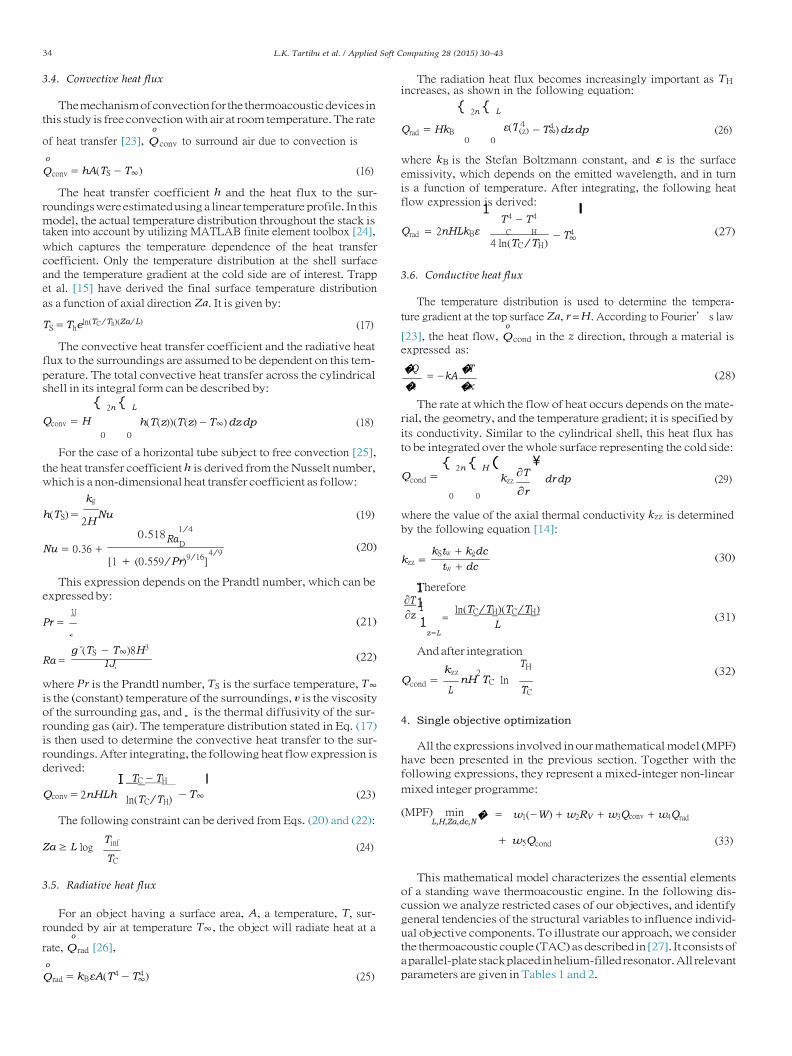
3.4. Convective heat flux
The mechanism of convection for the thermoacoustic devices in
this study is free convection with air at room temperature. The rate
The radiation heat flux becomes increasingly important as TH
increases, as shown in the following equation:
{ 2n { L
o
of heat transfer [23], Q conv to surround air due to convection is Qrad = HkB
0
4 (z)
0
− T 4 ) dz dp (26)
o
Q conv = hA(TS − T∞) (16)
The heat transfer coefficient h and the heat flux to the sur-
roundings were estimated using a linear temperature profile. In this
model, the actual temperature distribution throughout the stack is
where kB is the Stefan Boltzmann constant, and ε is the surface
emissivity, which depends on the emitted wavelength, and in turn
is a function of temperature. After integrating, the following heat
flow expression is derived: 1
T 4 − T 4 l
taken into account by utilizing MATLAB finite element toolbox [24], Qrad = 2nHLkBε C H − T 4 (27)
which captures the temperature dependence of the heat transfer
coefficient. Only the temperature distribution at the shell surface
and the temperature gradient at the cold side are of interest. Trapp
et al. [15] have derived the final surface temperature distribution
as a function of axial direction Za. It is given by:
TS = Theln(TC /Th)(Za/L) (17)
The convective heat transfer coefficient and the radiative heat
flux to the surroundings are assumed to be dependent on this tem-
4 ln(TC/TH)
3.6. Conductive heat flux
The temperature distribution is used to determine the tempera-
ture gradient at the top surface Za, r = H. According to Fourier s law o
[23], the heat flow, Q cond in the z direction, through a material is
expressed as:
perature. The total convective heat transfer across the cylindrical �Q �T
= −kA (28)
shell in its integral form can be described by: �t �x
Qconv = H
{ 2n { L
h(T (z))(T (z) − T∞) dz dp (18)
The rate at which the flow of heat occurs depends on the mate-
rial, the geometry, and the temperature gradient; it is specified by
0 0 its conductivity. Similar to the cylindrical shell, this heat flux has
For the case of a horizontal tube subject to free convection [25], to be integrated over the whole surface representing the cold side:
the heat transfer coefficient h is derived from the Nusselt number,
which is a non-dimensional heat transfer coefficient as follow:
Qcond =
{ 2n { H (
kzz ∂T
\
dr dp (29)
0 0 ∂r kg
h(TS) = 2H
Nu (19)
0.518 1/4
where the value of the axial thermal conductivity kzz is determined
by the following equation [14]:
Nu = 0.36 + D
[1 + (0.559/Pr)9/16
]
4/9 (20)
kzz = kStw + kgdc
tw + dc
(30)
This expression depends on the Prandtl number, which can be
expressed by: Therefore
1J Pr = ˛
(21)
∂T 1
1 =
∂z 1
1z=L
ln(TC /TH )(TC /TH )
L (31)
Ra = gˇ(TS − T∞)8H3
1J˛
(22) And after integration
kzz 2
TH
(32)
where Pr is the Prandtl number, TS is the surface temperature, T∞
is the (constant) temperature of the surroundings, v is the viscosity
of the surrounding gas, and ̨ is the thermal diffusivity of the sur-
Qcond = nH TC ln L TC
rounding gas (air). The temperature distribution stated in Eq. (17)
is then used to determine the convective heat transfer to the sur-
roundings. After integrating, the following heat flow expression is
derived: TC − TH
4. Single objective optimization
All the expressions involved in our mathematical model (MPF)
have been presented in the previous section. Together with the
following expressions, they represent a mixed-integer non-linear
Qconv = 2nHLh
I ln(TC/TH)
− T∞l
(23) mixed integer programme:
The following constraint can be derived from Eqs. (20) and (22):
Za ≥ L log Tinf
(24)
TC
(MPF) min L,H,Za,dc,N
� = w1(−W ) + w2RV + w3Qconv + w4Qrad
+ w5Qcond (33)
3.5. Radiative heat flux
For an object having a surface area, A, a temperature, T, sur-
rounded by air at temperature T∞, the object will radiate heat at a o
rate, Q rad [26],
o
Q rad = kBεA(T 4 − T 4 ) (25)
This mathematical model characterizes the essential elements
of a standing wave thermoacoustic engine. In the following dis-
cussion we analyze restricted cases of our objectives, and identify
general tendencies of the structural variables to influence individ-
ual objective components. To illustrate our approach, we consider
the thermoacoustic couple (TAC) as described in [27]. It consists of
a parallel-plate stack placed in helium-filled resonator. All relevant
parameters are given in Tables 1 and 2.

L.K. Tartibu et al. / Applied Soft Computing 28 (2015) 30–43 35
V
Table 1
Specifications for thermoacoustic couple.
Parameter Symbol Value Unit
Table 4
Optimal solutions minimizing viscous resistance.
L* H* Za* dc* N* R∗
CPU time (s)
Isentropic coefficient v 1.67
Gas density p 0.16674 kg/m3
Specific heat capacity cp 5193.1 J/kg K
Dynamic viscosity µ 1.9561 × 10⁻⁵ kg/m s
x* 0.005 0.008 0.005 5.8140E−4 20 3.467 1.062
• increasing the number of channels (N* = Nmax) and the channel
diameter d so that we maximize the thermoacoustically active
surface area,
• setting N* = Nmax and dc* = dcmax ensures that H can take its max-
imum value in constraint (6).
Isobaric specific heat capacity cp 5193.1 J/(kg K)
Table 2
Additional parameters used for programming.
Parameter Symbol Value Unit
Temperature of the surrounding T∞ 298 K
4.2. Emphasizing viscous resistance
We emphasize RV by setting objective function weights
w1 = w3 = w4 = w5 = 0 and w2 = 1. The problem then simplifies to Eqs.
(2) and (15), constraints (6) and (24), and variable restrictions (34).
Objective function (33) becomes:
Constant cold side temperature TC 300 K
Constant hot side temperature TH 700 K
Wavelength 1.466 m
min L,H,dc,Za,N
�RV = RV (36)
Thermal expansion ˇ 1/T∞ 1/K
Thermal diffusivity ˛ 2.1117E−5 m2 s−1
In Table 4, the optimal solutions that minimize �RV are repre-
sented with letter subscripted with asterisk.
Physically, this optimal solution can be interpreted as:
4.1. Emphasizing acoustic work
• making the stack as small as possible (L* = Lmin
), therefore reduc-
All proposed models MINLP are solved by GAMS 23.8.1 [19],
using LINDOGLOBAL solver on a personal computer Pentium IV
1.6 GHz with 0.99 GB RAM. The following constraints (upper and
lower bounds) have been enforced on variables in other for the
solver to carry out the search of the optimal solutions in those
ranges:
L.lo = 0.005; L.up = 0.05;
Za.lo = 0.005; Za.up = 0.050;
ing the individual (viscous) resistance of each channel to its
minimum,
• moving the stack as near as possible to the closed end
(Za* = Zamin), • decreasing the number of channels (N* = Nmin).
• setting N* = Nmin and dc* = dcmin ensures that H can take its mini-
mum value in constraint (6).
4.3. Emphasizing convective heat flux
N.lo = 20; N.up = 50;
H.lo = 0.005; H.up = 0.050;
dc.lo > 2.ık; dc.up < 4.ık [10]
(34)
We can emphasize Qconv by setting objective function weights
w1 = w2 = w4 = w5 = 0 and w3 = 1. The problem then reduces to Eqs.
(17), (19) and (20) (22), constraints (6) and (24) and variable
Setting the objective function weights to w2 = w3 = w4 = w5 = 0 restrictions (34). Objective function (33) becomes:
and w2 = 1, the problem reduces to Eqs. (1) (3), (9) and (11) (13),
constraints (6) and (24) and variable restrictions (34). Objective function (33) becomes:
min L,H,dc,Za,N
�Qconv = Qconv (37)
min L,H,dc,Za,N
�W = (−W ) (35)
In Table 5, the optimal solutions that minimize �Qconv are repre- sented with letter subscripted with asterisk.
Physically, this optimal solution can be interpreted as:
In our approach, the geometry range is small in order to illustrate
the behaviours of the objective functions and optimal solution of a
small-scale thermoacoustic engine. In Table 3, the optimal solu-
tions that maximize �W are represented with letter subscripted
with asterisk.
Physically, this optimal solution can be interpreted as:
• making the stack as long as possible (L* = Lmax),
• making the stack wide,
• moving the stack as near as possible to the closed end (Za* = Zamin)
maximizing the available pressure amplitude for the thermody-
namic cycle and thus work output W and,
Table 3
Optimal solutions maximizing acoustic work.
• making the stack as large as possible (L* = Lmax),
• moving the stack as near as possible to the closed end
(Za* = Zamin), • decreasing the number of channels (N* = Nmin),
• setting N* = Nmin and dc* = dcmin ensures that H can take its mini-
mum value in constraint (6).
4.4. Emphasizing radiative heat flux
We can emphasize Qrad by setting objective function weights
w1 = w2 = w3 = w5 = 0 and w4 = 1, so that only Eq. (27), constraints
Table 5
Optimal solutions minimizing convective heat flux.
L* H Za*
dc* N* W* CPU time (s)
L* H* Za* dc* N* Q ∗ CPU time (s) conv
x* 0.050 0.034 0.005 0.001 50 4.5536E+9 18.171 x* 0.005 0.008 0.005 5.93522E−4 20 0.1623 0.718
Maximum velocity umax 670 m/s
Maximum pressure pmax 114,003 Pa
Speed of sound
Thickness plate
Frequency
c
tw
f
1020
1.91 × 10⁻⁴
696
m/s
m
Hz
Thermal conductivity helium kg 0.16 W/(m K)
Thermal conductivity stainless steel kS 11.8 W/(m K)

36 L.K. Tartibu et al. / Applied Soft Computing 28 (2015) 30–43
Q
i i i
.
2 −
2 −
( f − f
\
Q
. ⎟ .
.
⎟ ⎟ ⎟ .
Table 6
Optimal solutions minimizing radiative heat flux. while the other objectives are added as constraints to the feasible
solution space of • as follows:
L* H* Za* dc* N* ∗
rad CPU time (s) SOe(X) = min(f1(x))
x* 0.005 0.008 0.005 5.93522E−4 20 0.7305 5.750
subject to x ˝
(40)
(6) and (24) and variable restrictions (34) are active. For these
restricted optimization problems, objective function (33) becomes
f2(x) ≤ ε2, f3(x) ≤ ε3, . . ., fp(x) ≤ εp, x ̋
By solving iteratively problem SOe(X) for different values of εp,
different Pareto solutions can be obtained. The range of at least
min L,H,dc,Za,N
�Qrad = Qrad (38) p − 1 objectives functions is necessary in order to determine grid
points for ε1, . . ., εp values and apply the ε-constraint method.
The most common approach is to calculate these ranges from the In Table 6, the optimal solutions that minimize �Qrad
are repre- sented with letter subscripted with asterisk:
Physically, this optimal solution can be interpreted as:
• making the stack as large as possible (L* = Lmax),
• moving the stack as near as possible to the closed end
(Za* = Zamin), • decreasing the number of channels (N* = Nmin),
• setting N* = Nmin and dc* = dcmin ensures that H can take its mini-
mum value in constraint (6).
payoff table (Fig. 5). Each objective function is optimized individ-
ually. The mathematical details of computing payoff table for a
multi-objective mathematical programming (MMP) problem can
be found in Cohon [28]. The payoff table for a MMP problem with
(p) competing objective functions is calculated as follow:
• The individual optima of the objective functions (fi) are calcu-
lated. The optimum value of the objective functions (fi) and the vector of decision variables which optimizes the objective func-
tion (fi) are indicated respectively by f ∗(x∗
) and x∗
. • Represent the payoff table including f ∗(x∗
), f ∗(x∗
), . . ., f ∗(x∗
) as
4.5. Emphasizing conductive heat flux follows: 1 1 2 2i p p
⎛ f ∗(x
∗ ) · · · f ∗(x
∗ ) · · · f ∗(x
∗ )
We emphasize Qcond by setting objective function weights
w1 = w2 = w3 = w4 = 0 and w5 = 1, so that only Eqs. (30) and (32),
constraints (6) and (24) and variable restrictions (34) are active.
1 1 i 1 p 1 ⎟ . . . .
⎟ ⎟
. . .
⎟ ⎟ Objective function (33) becomes: ˚ =
⎟ f ∗ ∗ ∗ ∗
∗ ∗ ⎟ ⎟
1 (xi ) · · · fi
(xi ) · · · fp (xi ) ⎟ (41)
min L,H,dc,Za,N
�Qcond = Qcond (39)
⎟
⎟ ⎟ .
. . . .
. ⎠
f ∗ ∗ ∗ ∗ ∗ ∗
In Table 7, the optimal solutions that minimize �Qcond are repre-
sented with letter subscripted with asterisk.
Physically, this optimal solution can be interpreted as:
• making the stack as large as possible (L* = Lmax),
• moving the stack as near as possible to the closed end
(Za* = Zamin), • decreasing the number of channels (N* = Nmin),
1 (xp) · · · fi
(xp) · · · fp (xp)
• Determine the range of each objective function in the payoff table
based on utopia and pseudo-nadir points. The Utopia point (fU)
refers to a specific point where all objectives are simultaneously
at their best possible values. It is generally outside the feasi-
ble region. However, the Nadir point (fSN) is a point where all
objective functions are simultaneously at their worst values. It is
generally in the objective space
• setting N* = Nmin and dc* = dcmin ensures that H can take its mini- f U ≤ fi (x) ≤ f SN (42)
i i
mum value in constraint (6).
5. The proposed MMP solution approach to emphasize all
objective components
In order to introduce the proposed MMP solution approach
applied to this study, at first a brief review of the ε-constraint
technique is presented.
5.1. ε-Constraint method
• Divide the range of p − 1 objectives functions f2, . . ., fp to q2, . . .,
qp into equal intervals using (q2 − 1), . . ., (qp − 1) intermediate equidistant points, respectively. p
• Convert the MMP problem into n
(qi + 1) single objective opti-
i=2
mization sub-problems as follows:
min f1(x)
subject to
f2(x) ≤ ε2,n2, . . ., fp(x) ≤ εp,np
In this method, the decision maker specifies the trade-off among
multiple objectives. This method is also known as the trade-off
method, or reduced feasible space • method, because the tech-
( f SN − f U
\ ε2,n2 = f SN 2 2
q2 × n2, n2 = 0, 1, . . ., q2
(43)
nique involves a search in a progressively reduced criterion space.
The original problem is converted to a new problem in which one
objective (or single objective SO) is minimized (or maximized)
ε2,n2 = f SN
SN U 2 2
q2 × n2, n2 = 0, 1, . . ., q2
Table 7
Optimal solutions minimizing conductive heat flux.
• Each sub-problem is a candidate solution or Pareto optimal solu-
tion of the MMP problem. At the same time, some of these
optimization sub-problems may have infeasible solution space
due to the added constraints for f2, . . ., fp; such sub-problems are
L* H* Za* dc* N* ∗
cond CPU time (s) discarded.
• Selection of the most preferred solution out of the obtained Pareto x* 0.050 0.008 0.005 5.8140E−4 20 2.8951 0.656 optimal solutions by the decision maker.

L.K. Tartibu et al. / Applied Soft Computing 28 (2015) 30–43 37
Adapted from [29].
Fig. 5. Flowchart of the lexicographic optimization for calculation of payoff table.
The detailed explanation of the algorithm can be found in
Ehrgott [30]. technique [31,32]. Therefore, the augmented ε-constraint
method can be formulated as follows:
5.2. Augmented ε-constraint method
min
( f1(x) − ı
( s2
r2
+ s3
r3
+ · · · + sp
\\
rp
(44) subject to
In the ordinary ε-constraint method, the efficiency of Pareto solutions is not guaranteed. Inefficient solutions can be generated.
The obtained solution is considered inefficient if there is another
Pareto solution that can improve at least one objective function
without deteriorating the other objectives functions. In order to
overcome this drawback, we consider the following:
a. The objective functions constraints in Eq. (43) are trans-
formed into equality constraints by means of the slack variable
f2(x) + s2 = ε2, . . ., fp(x) + sp = εp s2, . . ., sp R+
where s2, . . ., sp represent the slack variables for the constraints
in Eq. (43) of the multi-objective mathematical programming
(MMP) problem and ı is a small number usually between
10−3 and 10−6 [33]. This formulation (Eq. (44)), preventing the
generation of an inefficient solution, is known as augmented
ε-constraint method due to the augmentation of the objective
function (f1) by the second term. Its proof can be found in [33].

38 L.K. Tartibu et al. / Applied Soft Computing 28 (2015) 30–43
2
1
1
Adapted from [29].
Fig. 6. Flowchart of AUGMENCON method for optimization.
b. The concept of relative importance of objective in generating the
Pareto solutions is introduced to be consistent with the deci-
sion maker policy. Although each objective has its own relative
in order to keep the solution of the first optimization. Assume
that we obtain min f2 = x∗ . Subsequently, the constraints f1 =
x∗ and f2 = x∗ are added to optimize the third objective func- 1 2
importance in the MMP problem, the previous formulations con-
sider all slack variables with equivalent importance. In MMP
problems, the concept of optimality stipulates that we search
for the most preferred solution among the generated Pareto set.
To remedy the inconsistency in the decision making process, the
formulation of the augmented ε-constraint method is modified
by the use of a lexicographic optimisation of these series of objec-
tive functions. Practically, the first objective function of higher
priority is optimized, obtaining min f1 = x∗ . Then the second
objective function is optimized by adding the constraint f1 = x∗
tion in order to keep the previous optimal solutions and so on, until all objective functions are dealt with. The flowchart of the
lexicographic optimization of a series of objective functions is
illustrated in Fig. 6.
By the combination of the lexicographic optimization and aug-
mented ε-constraint method, the range of the objective functions
in the payoff table is optimized and results in the generation of only
efficient solutions within the identified ranges. This is illustrated by
the flowchart in Fig. 6.

L.K. Tartibu et al. / Applied Soft Computing 28 (2015) 30–43 39
The proposed augmented ε-constraint method is expected to
provide a representative subset of the Pareto set which in most
augmented ε-constraint method for solving model (Eq. (40)) can be
formulated as follows:
cases is adequate. The basic step towards further penetration of
the generation methods in our multi-objective mathematical prob-
lems is to provide appropriate codes in a GAMS environment and
produce efficient solutions.
5.3. Model implementation
Lastly, we simultaneously consider all five objective com-
ponents by regarding acoustic work W, viscous resistance RV,
convective heat flux Qconv, radiative heat flux Qrad and conductive
max W(L,H,Za,dc,N) + dir1r1 ×
r2
subject to
RV(L,H,Za,dc,N) − dir2s2 = ε2
Qconv(L,H,Za,dc,N) − dir3s3 = ε3
Qrad(L,H,Za,dc,N) − dir4s4 = ε4
Qconv(L,H,Za,dc,N) − dir5s5 = ε5
si ℜ+
+ s3
r3 +
s4
r4 +
s5
r5
(46)
heat flux Qcond as five distinct objective components. All the expres-
sions involved in the multi-objective mathematical programming
(MMP) have been presented in the previous section. The optimiza-
tion task is formulated as a five-criteria mixed-integer non-linear
programming problem (MPF) that simultaneously minimize the
negative magnitude of the acoustic work W (since it is the only
objective to be maximized), the viscous resistance RV, the convec-
tive heat flux Qconv, the radiative heat flux Qrad and the conductive
heat flux Qconv.
where diri is the direction of the ith objective function, which is
equal to −1 when the ith function should be minimized, and equal
to +1, when it should be maximized. Efficient solutions of the prob-
lem are obtained by parametrical iterative variations in the εi. Si
are the introduced surplus variables for the constraints of the MMP
problem. r1si/ri is used in the second term of the objective function,
in order to avoid any scaling problem. The formulation of Eq. (41) is
known as the augmented ε-constraint method due to the augmen-
tation of the objective function W by the second term. The following
constraints (upper and lower bounds) have been enforced on vari-
(MPF) min L,H,Za,dc,N
� = {−W(L,H,Za,dc,N), RV (L,H,Za,dc,N), ables in other for the solver to carry out the search of the optimal
solutions in those ranges:
Qconv(L,H,Za,dc,N), Qrad(L,H,Za,dc,N), Qcond(L,H,Za,dc,N)} (45)
Subject to constraints (6), (24) and (47).
In this formulation, (L, H, Za, dc, N) denotes the geometric
L.lo = 0.005; L.up = 0.05;
Za.lo = 0.005;
H.lo = 0.005;
dc.lo > 2.ık; dc.up < 4.ık
(47)
parameters.
There is no single optimal solution that simultaneously opti-
mizes all the five objectives functions. In these cases, the
decision makers are looking for the most preferred solu-
tion. To find the most preferred solution of this multi-objective
model, the augmented ε-constraint method (AUGMECON) as pro-
posed by Mavrotas [33] is applied. The AUGMECON method
has been coded in GAMS. The code is available in the GAMS
library (http://www.gams.com/modlib/libhtml/epscm.htm) with
an example. While the part of the code that has to do with the
example (the specific objective functions and constraints), as well
as the parameters of AUGMENCON have been modified in this case,
the part of the code that performs the calculation of payoff table
with lexicographic optimization and the production of the Pareto
optimal solutions is fully parameterized in order to be ready to
use.
Practically, the ε-constraint method is applied as follows: from
the payoff table the range of each one of the p − 1 objective func-
tions that are going to be used as constraints is obtained. Then
the range of the ith objective function to qi equal intervals using
(qi − 1) intermediate equidistant grid points is divided. Thus in
total (qi + 1) grid points that are used to vary parametrically the
right hand side (εi) of the ith objective function is obtained. The
total number of runs becomes (q2 + 1) × (q3 + 1) × . . . × (qp + 1). The
ε-constraint method has several important advantages over tradi-
tional weighted method. These advantages are listed in Mavrotas
[33]. In the conventional ε-constraint method, there is no guaran-
tee that the obtained solutions from the individual optimization of
the objective functions are Pareto optima or efficient solutions. In
order to overcome this deficiency, the lexicographic optimization
for each objective functions to construct the payoff table for the
multi-objective mathematical programming (MMP) is proposed in
order to yield only Pareto optimal solutions (it avoids the genera-
tion of weakly efficient solutions) [29]. The mathematical details of
computing payoff table for MMP problem can be found in [29]. The
We use lexicographic optimization for the payoff table; the
application of model (Eq. (46)) will provide only the Pareto optimal
solutions, avoiding the weakly Pareto optimal solutions. Efficient
solutions of the proposed model have been found using AUGMEN-
CON method and the LINDOGLOBAL solver. To save computational
time, the early exit from the loops as proposed by Mavrotas [23] has
been applied. The range of each five objective functions is divided in
four intervals (5 grid points). The integer variable N has been given
values from 20 to 50. This process generates optimal solutions cor-
responding to each integer variable. The maximum CPU time taken
to complete the results is 1029.700 s. The following section report
only sets of Pareto solutions obtained:
Fig. 7 represents the Pareto optimal solutions graphically; it
shows that there is not one single optimal solution that opti-
mizes the geometry of the stack and highlights the fact that the
geometrical parameters are interdependent, supporting the use
of a multi-objective approach for optimization of thermoacoustic
engines. To maximize acoustic work W and minimize viscous resis-
tance and thermal losses simultaneously, there is a specific stack
length (L) to which correspond a specific stack height (H), a spe-
cific stack spacing (dc) and a specific number of channels (N). This
study highlights the fact that the geometrical parameters are inter-
dependent, which support the use of a multi-objective approach
for optimization. It should be noted that in all cases, locating the
stack closer to the closed end produced the desired effect. All Pareto
optimal solutions can be identified to reinforce the decision maker s
final decision and preferred choice.
These optimal solutions are then used to construct Figs. 8 10
representing respectively acoustic work, viscous resistance, con-
ductive, and thermal losses plotted as a function of N, L, dc and
H.
It can be seen that there is a similar trend for acoustic work when
considering the number of channels N and the stack height H with
the maximum values expected respectively for N = 43 (Fig. 8a) and
H = 0.028 (Fig. 8d). The results obtained for the stack length and the
s2

L.K. Tartibu et al. / Applied Soft Computing 28 (2015) 30–43 41
V
Fig. 7. Optimal structural variables.
stack spacing suggest to increase the stack length to Lmax (Fig. 8b)
or decrease the stack spacing to dcmin (dc = 2ık) (Fig. 8c) in order to
maximize the acoustic work.
The viscous resistance results show that minimal values are
expected by maximizing number of channels (N = 42) (Fig. 9a) and
increasing the stack height (H = 0.028) (Fig. 9d). Minimal values of
viscous resistance function of the stack length and the stack spac-
ing are observed by decreasing the stack length (L = 0.005) (Fig. 9b)
5.4. Results comparison
An alternative way to simultaneously maximize acoustic work
and minimize losses (viscous resistance as well as heat flows) is
to consider the thermal efficiency (17) which can be defined as the
ratio of the work output over the sum of the work output and losses
as follows:
W and increasing the stack spacing to dcmax (dc = 4ık) (Fig. 9c).
The analyses of results obtained for the conductive, convec-
17 = W + RV + Qconv + Qrad + Qcond
(48)
tive and radiative heat fluxes show a similar trend. An increase in
number of channels, stack spacing and stack height result in a sim-
ilar increase of these thermal losses with minimal values observed
when geometrical parameters are minimized (Fig. 10a, c and d).
However, the influence of the stack length show a different trend
with minimal value observed for L = 0.047 (Fig. 10b).
The viscous resistance in Eq. (15) has the units [kg/m4 s]. In order
to express this in terms similar to the other variables used in Eq.
(48), we multiply Eq. (15) (subsequently R∗ in Table 10) by the vol-
umetric velocity [m3/s] and the oscillating frequency [1/s], yielding
[W/m] as final unit for the viscous resistance per channel used in
Eq. (48). This ratio can be used to compare the results obtained
Fig. 8. Acoustic power plotted as a function of N, L, dc and H.

40 L.K. Tartibu et al. / Applied Soft Computing 28 (2015) 30–43
Fig. 9. Viscous resistance plotted as a function of N, L, dc and H.
by the proposed augmented ε-constraint method and identify the
preferred solution. These solutions are presented in Table 11. For
the sake of conciseness, optimal solutions with identical number
of channels obtained with ordinary ε-constraint method (Table 11)
are compared to solutions obtained with the proposed method
(Table 10) to demonstrate the efficiency of the solutions obtained
with the proposed method (Fig. 11).
Based on the magnitude of work output, viscous resistance
and heat fluxes, these results suggest that the solution reported
in Table 10 corresponding to 42 and 43 channels are the best
Fig. 10. Conductive, convective and radiative heat fluxes plotted as a function of N, L, dc and H.

L.K. Tartibu et al. / Applied Soft Computing 28 (2015) 30–43 43
V Q Q Q
V Q Q Q
Table 10
Non-dominated solutions found by AUGMENCON.
N L* dc* H* Za* W* R∗
∗ cond
∗ conv
∗ rad
CPU time (s)
21 Channels 0.047 0.00098521 0.012 0.005 13752.67 671.112 1.803 9.301 1.312 1029.700
25 Channels 0.043 0.00100000 0.016 0.005 23061.14 292.007 3.010 10.230 1.552 1024.989
26 Channels 0.043 0.00100000 0.017 0.005 25924.46 243.410 3.367 10.464 1.614 1017.766
35 Channels 0.044 0.00100000 0.022 0.005 63219.01 110.627 5.783 13.081 2.171 47.409
36 Channels 0.045 0.00100000 0.022 0.005 68794.08 113.043 5.790 13.461 2.233 94.506
37 Channels 0.047 0.00097718 0.022 0.005 74687.64 125.216 5.557 13.927 2.295 118.498
42 Channels 0.040 0.00100000 0.028 0.005 108740.00 47.243 9.780 14.533 2.594 446.288
43 Channels 0.049 0.00092090 0.024 0.005 117420.00 97.351 6.763 15.798 2.672 386.976
Table 11
Solutions found by ordinary ε-constraint method.
N L* dc* H* Za* W* R∗
∗ cond
∗ conv
∗ rad
21 Channels 0.005 9.73E−04 0.012 0.005 1446.994 73.615 1.975 0.407 0.138
25 Channels 0.005 6.33E−04 0.010 0.005 1730.644 123.442 16.401 0.218 0.117
26 Channels 0.005 6.00E−04 0.010 0.005 1865.801 123.67 17.031 0.223 0.116
35 Channels 0.005 5.81E−04 0.014 0.005 4445.136 54.421 30.103 0.045 0.153
36 Channels 0.005 5.81E−04 0.014 0.005 4837.137 50.011 31.848 0.045 0.157
37 Channels 0.005 5.81E−04 0.014 0.005 5251.533 46.065 33.642 0.045 0.161
42 Channels 0.005 7.52E−04 0.020 0.005 9.38E+03 17.300 53.546 0.564 0.224
43 Channels 0.005 6.70E−04 0.019 0.005 9192.205 21.164 50.976 0.539 0.209
Fig. 11. Pareto solutions comparisons.
solutions for this application. As seen from Fig. 11, the augmented
ε-constraint produces more efficient candidate solutions and so
the decision maker can select a better final solution among the
generated Pareto sets.
6. Conclusion
Optimization as a design aid is required for thermoacoustic
engine to be competitive on the current market. Previous stud-
ies have relied heavily upon parametric studies. This work targets
the geometry of the thermoacoustic stack and uses multi-objective
optimization approach to find the optimal set of geometrical
parameters that optimizes the device. Five different parameters
(stack length, stack height, stack placement, stack spacing and
number of channels) describing the geometry of the device have
been studied. Five different objectives have been identified; a
weight has been given to each of them to allow the designer to
place desired emphasis. A mixed-integer non-linear programming
problem for thermoacoustic stack has been implemented in GAMS.
We have determined design statements for the each single objec-
tive emphasis case. For the case of multiple objectives considered
simultaneously, we have applied an improved version of a multi-
objective solution method, i.e., the epsilon constraint method called
augmented epsilon constraint method (AUGMENCON). This pro-
cess generates optimal solutions which are then use to illustrate
the conflicting nature of objective functions. The results found
shows the interdependence between the geometrical parameters
of the stack which support the use of our multi-objective approach
to optimize the geometry of thermoacoustic engine. The magni-
tude of acoustic work, viscous resistance and thermal losses are
computed for all optimal solutions and guidance is provided to
minimize thermal losses unlike previous studies. This is useful for
electronic cooling application where the magnitude of these ther-
mal losses is expected to increase. The proposed method not only
gives the efficient solutions corresponding to the optimal thermoa-
coustic engine stack geometry but also results in solutions that are
more preferred than those obtained using the ordinary ε-constraint
technique.